An adaptive estimator for registration in augmented reality

1

Second IEEE and ACM Int'l Workshop on Augmented Reality (IWAR) '99, Oct 20-21, 1999, San Francisco, CA (USA)

An Adaptive Estimator for Registration in Augmented Reality

Lin Chai, Khoi Nguyen (*), Bill Hoff, Tyrone Vincent Colorado School of Mines Golden, Colorado

(*) SymSystems, LLC Englewood, Colorado

(lchai,whoff,tvincent)@mines.edu

(*) [email protected]

Abstract In augmented reality (AR) systems using head-

mounted displays (HMD's), it is important to accurately sense the position and orientation (pose) of the user's head with respect to the world, in order that graphical overlays are drawn correctly aligned with real world objects. It is desired to maintain registration dynamically (while the person is moving their head) so that the graphical objects will not appear to lag behind, or swim around, the corresponding real objects. We present an adaptive method for achieving dynamic registration which accounts for variations in the magnitude of the users head motion, based on a multiple model approach. This approach uses the extended Kalman filter to smooth sensor data and estimate position and orientation.

1 Introduction In augmented reality (AR) systems using head-mounted

displays (HMD's), it is important to accurately sense the position and orientation (pose) of the user's head with respect to the world, in order that graphical overlays are drawn correctly aligned with real world objects. Even small errors in alignment (fractions of a degree) can be easily noticed by users, as a displacement of the virtual objects from the real objects on the HMD. The development of sensors that can accurately measure head pose remains a key technical challenge for AR.

Even if sensors can measure head pose accurately in a static situation (when the person is still), we still would like to maintain registration dynamically (while the person is moving their head). Otherwise, the graphical objects will appear to lag behind, or swim around, the corresponding real objects. This is annoying to users and tends to destroy the illusion that the virtual objects are co-existing with the real objects. Since people can move quite rapidly, fast sensors are needed.

A common approach to sensing rapid head motion is to use inertial sensors, such as linear accelerometers and angular rate gyroscopes that are mounted on the head.

These can be sampled at a very high rate, and are lightweight and portable. However, since these sensors can only measure the rate of motion, their signals must be integrated to produce position or orientation. The output of an accelerometer must be integrated twice to yield position, and the output of a gyroscope must be integrated once to yield orientation. Since the sensors are noisy, this leads to a drift in the estimated pose, which grows with elapsed time. To correct this accumulated drift, it is necessary to periodically reset the estimate of head pose, with a measurement from a sensor that can provide absolute pose information.

Absolute pose sensors have been developed using mechanical, magnetic, acoustic, and optical technologies [1]. Of these, optical sensors (such as cameras and photo-effect sensors) appear to have the best overall combination of speed, accuracy, and range [2] [3] [4]. One approach is to use active targets such as LED's that are mounted on the head and tracked by external sensors [5], or mounted in the world and tracked by head-mounted sensors [2]. Another approach is to use passive targets, instead of active targets. With this approach, head-mounted cameras and computer vision techniques are used to track fiducial targets (e.g., circular markings) or naturally occurring features in the scene [6]. However, computer vision techniques are computationally expensive, and therefore the update rate from a vision sensor may be much slower than from inertial sensors. A hybrid system consisting of a vision system and an inertial sensor system can overcome the problems of inertial sensor drift and slow vision sensor measurements [7]. Essentially, the inertial sensor system tracks head motion between vision sensor updates.

Even with a hybrid sensor system, it takes a finite amount of time to acquire inertial sensor data, filter it, compute head pose, and generate the graphical images that should be displayed for the new head pose. This delay between measurement and displaying the correct image may result in a large registration error if the person is moving - the virtual objects appear to lag behind the real objects. This error can be reduced by predicting head

2

motion [2]. The new image is generated corresponding to where we predict the head will be when the display gets updated.

A tool to predict head motion, as well as fuse inertial and vision sensor data, is the Kalman filter. The Kalman filter calculates the minimum variance state estimate given the correct description of zero mean white Gaussian noise and disturbances. It requires a model of how the system changes with time, and how measurements are related to the state. Since the maximum a-posteriori (MAP) estimate coincides with the minimum variance estimate for Gaussian distributions, the individual updates are MAP estimates with Bayesian priors. For a connection to least squares, the log-likelihood function for a MAP estimate is proportional to a quadratic cost function; thus given observations from k=1 to N, the Kalman filter finds the state trajectory of the system

kkk

kkk

DuHzyBuAzz

+=+=+1 (1)

which minimizes the cost function

2

11

211 −− −+− +

=∑ Qkk

N

kRkk AzzHzy (2)

subject to the dynamic constraints of equation (1). Finally, since the Kalman filter is the dual problem to

the linear quadratic regulator, it can be viewed as a “controller” which drives the state estimation error to zero. The extended Kalman filter expands the applications to nonlinear systems by linearizing around the estimated trajectory, and can be viewed as a suitable approximation to the above problems.

The extended Kalman filter and related estimators find extensive use in navigation systems since they are a natural way to fuse information from several asynchronous sensors. Indeed, if the sensor noise is independent, then each sensor can be incorporated using a separate measurement update, otherwise a lifted system must be used, or a decentralized approach.

Several researchers have used Kalman filters in augmented reality. For example, Azuma [2] uses a 10 state dynamic model of the HMD orientation that includes angular velocities and accelerations. For position, three independent filters are used, one for each axis. This approach requires some modeling of the typical motions that the HMD will experience with a human user. Foxlin [8] uses a different approach, called a complementary Kalman filter. Here, all errors are assumed to be captured by a bias in the inertial sensor, as well as measurement noise. In essence, an extended Kalman filter is designed using a dynamic model of the sensor bias behavior, rather than that of the HMD itself. Foxlin applied this to orientation measurements only. In this work, we do not address the problem of calibration or bias compensation. Rather, we assume that calibration of all sensors has been

accomplished, using a method such as Foxlin's, so that errors can be modeled as zero mean white noise.

In Kalman filters, it is important to set system parameters to yield optimal performance, specifically estimates of measurement noise and "process" noise. Measurement noise can usually be readily estimated by statistical analysis of sensor measurements taken off-line. However, process noise is more difficult to estimate. Process noise represents disturbances that are not captured in the process model. For example, if the state represented only angular velocity and not angular acceleration, then any non-zero angular accelerations would be considered as part of the process noise.

Normally, the noise parameters are chosen in order to make the filter converge quickly while damping out the effects of noise. However, the estimate of process noise that we should provide to the system may depend on the person's motion. For example, if the person is moving slowly, then effectively we have a small level of process noise. If the person is moving rapidly, accelerating quickly, etc, then we have a large level of process noise. If we can detect the type of motion that the person is performing, then we can customize the filter to optimize its performance.

In this paper, we describe a method to estimate filter parameters, based on the observed motion and the filter's performance. We use an adaptive estimation approach based on a multiple model estimator. We show that the adaptive approach results in improved prediction accuracy over a non-adaptive approach.

The rest of the paper is organized as follows. Section 2 describes the system model, including the state representation and system dynamics. Section 3 describes the method for adaptively selecting from among multiple models. Section 4 presents results on synthetic and actual data sets, and section 5 provides conclusions.

2 System Dynamics Our system consists of a see-through HMD (Virtual i-o

i-glasses) mounted on a helmet (Figure 1). Also attached to the helmet are three small video cameras (Panasonic GP-KS162, with 44-degree field of view). In this work, we used only two of the cameras. Also attached to the helmet is an inertial sensor system, consisting of a three-axis gyroscope (Watson Industries) and three orthogonally mounted single-axis accelerometers (IC Sensors).

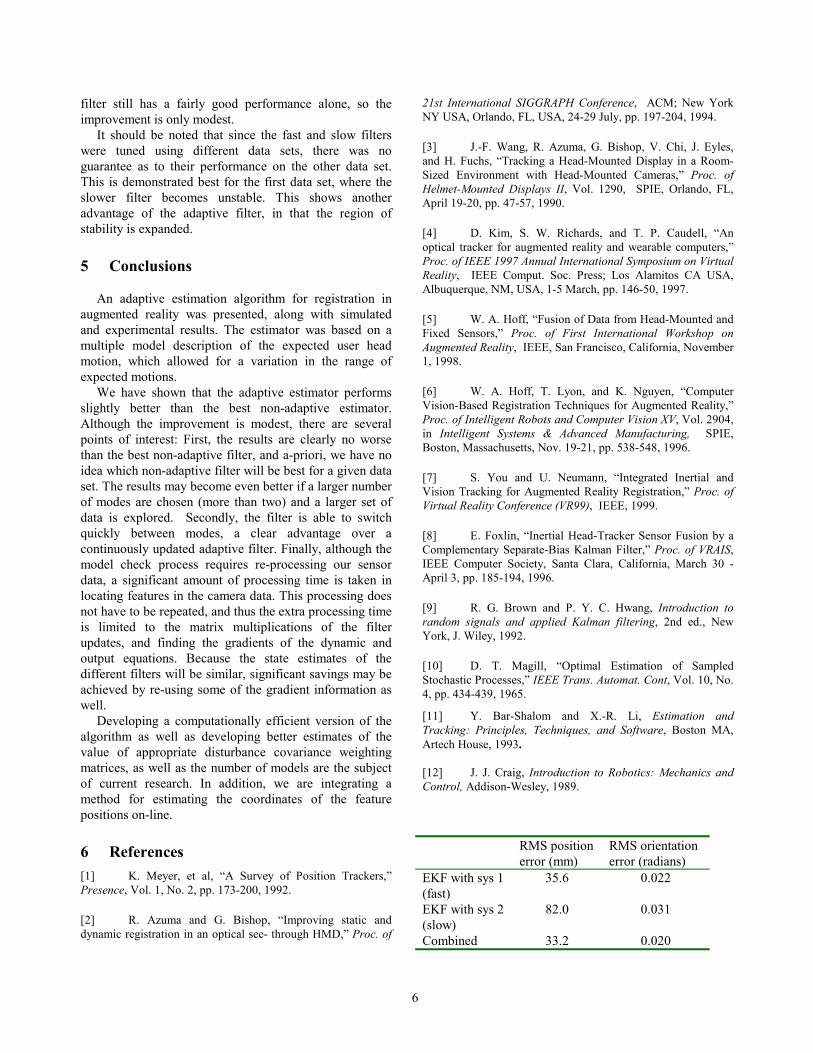
The frames of reference are given in Figure 2. The primary frame is the camera frame, which is approximately the center of rotation of the helmet. This allows a decoupling of the translation and orientation dynamics. The state z consists of the orientation of camera frame with respect to the world θ (we use Euler angles in this case, although quaternions can be used with

3

some modifications), the angular velocity Ω , the position x , the velocity x! , and the acceleration x!! of the camera frame with respect to the world.

With these states, the discretized system dynamics are as follows:

+

∆+∆+∆+

ΩΩ∆+

=

Ω

−

+

+

+

+

+

5

4

3

2

1

221

1

1

1

1

1

1 )(

k

k

k

k

k

k

kk

kkk

k

kk

k

k

k

k

k

wwwww

xxTx

xTxTx

TW

xxx

!!

!!!

!!!

!!

!

θθθ

(3)

where ∆T is the elapsed time since the previous time update, W is the Jacobian matrix relating Euler angles to angular velocity, and i

kw is an unknown input corresponding to the disturbance noise. These inputs come from the unknown motion of the user ( 52 , kk ww ), as well as from the linearization error. By grouping signals into vectors in the obvious way, we will use the notation:

kkk wzfz +=+ )(1 (4) Sensors have associated with them an output equation,

which maps the states to the sensor output, and an uncertainty in the output space. The output equations for each sensor are defined as follows. The gyroscope produces three angular velocity measurements, one for each axis (units are s

rad ), which are related to θ and θ! via [12]

θθ !)(Wyg = (5) The accelerometers produce three acceleration

measurements, one for each axis (units are 2smm ):

+×Ω+×Ω+

=

GPRdtdPRxR

y

ICW

CICW

CI

W

a

)()( θθ!!! (6)

where RWC is a matrix rotation from the camera C frame

to the W frame, RIW is the rotation from W to I,

and G is gravity. The computer vision system measures the image

position of a target point in the world, in each of the two cameras (units are mm). The cameras are separated by a distance d. Using the estimated world-to-camera pose, we transform the world point into camera coordinates, and then project it onto the images using the perspective projection equations. Here, f is the focal length of the camera lenses in mm, f

W P is the position of the feature

in the world frame which is considered known, and

CorgW P is the position of the C frame origin:

( )

( )

+=

−=

=

zy

zx

zy

zx

v

CorgW

fWC

W

z

y

x

fC

pppdp

pppp

fy

PPRppp

P )(θ

(7)

Each sensor has sensor noise associated with it, so the measurement at sample time k for the camera data is actually

vvk nyy += (8)

where vn is an unknown noise input associated with the computer vision. A similar relation holds for the inertial data. The sensor data varies in the amount of sensor noise, and the rate at which the data arrives. Typically, the data rates of the inertial sensors are much greater than the computer vision.

A statistical description of these unknown inputs and sensor noise in the form of a mean and covariance is used by the extended Kalman filter to determine the appropriate update weightings from the sensor data. That is, we assume that w and n are zero mean white Gaussian sequences with covariance

=

v

a

g

T

v

a

g

v

a

g

RR

RQ

nnnw

nnnw

E

000000000000

(9)

However, in our application, the size of Q will depend on the current activity. For example, if a user were working at a central location, we would expect the translational inputs to be small, with perhaps large orientation inputs. However, if the user is walking between rooms, the translational inputs will be larger, while the orientation inputs may be small. In order to accommodate different modes of operation, we will use a multiple model estimation scheme that is described below.

The extended Kalman filter (EKF) updates the state estimate kz and the associated state covariance matrix

kP as follows [9]:

Time Update: QPAAP

zfz

kkk

kk

+=

=−

−+ )ˆ(ˆ 1 (10)

4

Measurement Update:

kkk

kkkk

Tkkk

Tkk

PKHIPyyKzz

RHPHHPK

)()ˆ(ˆˆ

)(

1

11

1

−=−+=

+=

+

−++

−

(11)

where ky is the current observation (inertial or camera),

ky is the prediction of the sensor output given the current

state estimate, and kk HA , are the gradient of the dynamics equation and observation equation respectively at the current state estimate

3 Multiple Model Estimation Often a model is available but may have unknown

parameters, requiring adaptive estimation techniques to be applied. A useful approach to adaptive estimation is the so-called multiple model estimation. In this case, the system dynamics are unknown, but assumed to be one of a fixed number of known possibilities. That is, consider the set of models

)()(

)()(1

φφ

kkk

kkk

nzgywzfz

+=+=+ (12)

where x is the state, y is the output, w is a random disturbance and n is random measurement noise. The model is parameterized by φ which takes values in a finite set. It is assumed that the true system is captured by one of the models. This approach began with the work of Magill [10], who considered the problem under the usual linear/Gaussian assumptions. Magill derived the optimal least squares estimator, which consists of running several Kalman filters in parallel, the number of filters equal to the number of possible modes. The minimum variance state estimate is given by ∑=

j

kjjk YPzz ]|[ˆˆ φ (13)

where jz is the minimum variance estimate for model

j , and ]|[ kj YP φ is the probability that model j is

the correct model given kY , the measured data up to time k . The linear/Gaussian assumptions allow a recursive algorithm for the calculation of ]|[ k

j YP φ , which is a measure of the size of the prediction error residuals. Under mild assumptions, this probability will approach unity for the correct model as time increases. For more details, see for example [9]. This has been extended to linear systems which do not operate in a single mode, but

that can switch between modes during operation. Unfortunately, in this case we must compute the probabilities for all potential sequences of modes as time increases, which leads to an exponentially increasing computational burden; but practical approximations have been developed (see [11] for more details). In our case, we will be somewhat more ad-hoc in our development, since the system dynamics and output equations are nonlinear, and the input sequence caused by the user's motion is neither white nor Gaussian in general, so that even the computationally expensive linear-optimal algorithm does not apply. This is the main reason that the optimal solution, or other existing sub-optimal approaches such as Interacting Multiple Models [11] were not used. Indeed, in the nonlinear case, the covariance matrices must often be adjusted away from expected noise levels to ensure stability as well as performance, making statistical tests difficult to interpret. However, we are guided by two features of the existing algorithms: the best estimate is primarily from the system with the smallest weighted prediction error, and the prediction error should be measured over a short window to allow for mode switching.

A possible alternative to the multiple model approach would be an adaptive filter that can update the noise model in a continuous manner via a stochastic gradient descent algorithm. However, this approach requires choosing an update rate for the noise model parameters. If this rate is chosen too slow, then the adaptive filter cannot follow fast changes in the users behavior. If this update rate is chosen too fast, then the filter may become unstable.

For our application, the primary figure of merit is the accuracy by which the computer graphics are overlaid on the head mounted display. As a proxy for this, we will use the prediction error of the camera features to determine when to switch from one model to another. In our scheme, a decision is made to check the performance of the current filter. This decision could be made on the basis of reaching a threshold in the size of the prediction error, or could be done at set time intervals. At sample ck the prediction error over the last c camera measurements for the current filter is recorded, given by

∑Ω∈

−=k

kk yyPE ˆ (14)

where Ω is the set of indexes that correspond to the last c camera measurements. A fixed amount of data is selected, for example the last b samples, to be run through the alternative filter(s) with initial conditions given by the estimate and covariance of the currently selected filter at time bk − . The prediction error over the c camera measurements in that data are recorded, and the filter with the smallest prediction error is selected to

5

continue into the future. At this point, the current state estimate and error covariance matrix are re-set to the value obtained by the best filter. The performance check process is illustrated in Figure 3.

Note: in our implementation of the EKF, both the camera and gyro measurement updates are full order, in that both position and orientation (and associated derivatives) are modified. However, the accelerometer update considers the orientation to be fixed, and only updates the position part of the state matrix.

4 Results We first examine the behavior of the method on purely

synthetic data. A synthetic position and orientation are described, and synthetic accelerometer, gyro, and camera data are generated from it. A synthetic white Gaussian random sequence is added to the measurements with variance .01 for gyros, 1300 for accelerometers, and .0016 for the camera. These were chosen to be similar to existing sensors in our lab. The computer vision data assumed that 5 features were identified, located at points in space around the user. The data rates of the sensors are 10ms for the inertial sensors, and 100ms for the vision data.

The filter parameters were chosen as follows: [ ]( )[ ]( )IIIIIdiagQ

IIIIIdiagQ4

2

651

1011001001.0001.

101101101.001.×=

××=

where diag indicates the matrix is block diagonal with the listed elements along the diagonal and I is a 33× identity matrix. The noise matrices were chosen to be the same level as the synthetic noise. Note that one filter assumes that the motion will be much more restricted than the other.

First, the sensor data was run through the EKF using each model separately – no adaptation was performed. The results are shown in Figure 4, with the true position or orientation shown as a solid line, while the estimates are drawn with dashed lines. In Figure 4a is the orientation estimate for the EKF running with system 1 (expects larger disturbances, thus higher bandwidth), Figure 4b is the orientation estimate with system 2, Figure 4c is the position estimate for system 1, and Figure 4d is the position estimate for system 2. Note that the motion occurs over one axis in the first half of the data, while the “user” is holding still for the second half. As expected, the higher bandwidth filter (using system 1) follows the trajectory more closely, but has nosier estimates. The lower bandwidth filter (using system 2) has severe biases and overshoots, but the estimates are less noisy.

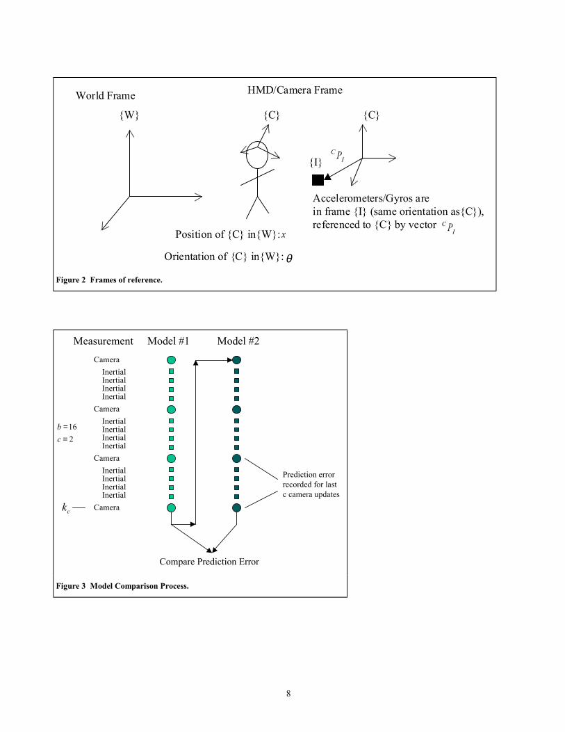
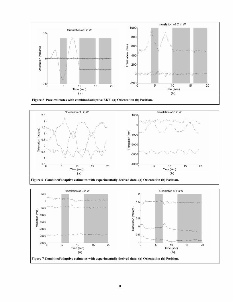
Next, the same data run through the adaptive filter that selects the model based on the camera data prediction error. The results are shown in Figure 5. The times in

which the filter used the system 1 model (high bandwidth) are clear, while the times in which system 2 was used (low bandwidth) are shaded. Note that the low bandwidth filter is used extensively, especially in the quiescent period, yet the biases are not evident. The dual filter selects the appropriate model for the current behavior. To quantify the improvement, we recorded the root mean square error of position and orientation prediction (average is over

time for all three axes, so divide by 3 to get per-axis error). The results are given in Table 1.

Although the improvement of the adaptive estimator is not terribly large over the EKF with system 1, it is quite a bit better than the EKF with system 2. This gives us a way of reducing the “jitter” in graphic overlays due to a higher variance position and orientation estimate while still following high bandwidth maneuvers.

The next data set we examined uses position and orientation data from an actual user of the head mounted display. One set of data had the user moving objects around the room, and thus had large movements, while the second data set was taken while the user performed a disassembly task, and contains smaller head motions. This data was collected using an infra-red tracking camera (Nothern Digital Optotrak) and is precise to .1 mm, and sampled at approximately 50 ms. This data was interpolated using splines, and then synthetic accelerometer, gyro and camera data was generated with added noise as above. The data rates of the sensors are 50ms for inertial sensors and 250ms for the vision data. Thus the motion is life like, although the sensor data is synthetic. We attempted to find a statistical estimate for the Q matricies by determining the variance of the difference between the actual states and what would be predicted by our linearized model. However, the filters designed were not stable, and we instead tuned the Q matricies by hand. One set of filter gains was tuned using the large head motions, and one set was tuned using the smaller head motions. The resulting gains were as follows: System 1:

[ ]( )IIIIIdiagQ

IRIRIR vag

1064 1011011011001.

16.130001.

×××=

===

System 2:

[ ]( )IIIIIdiagQ

IRIRIR vag

64

7

101105105.01.

16.103.101.

××=

=×==

The results for the first set of data are shown in Figure 6, and tabulated in Table 2. In this case, the slower filter used alone became unstable. Note that the filter always chooses to use the faster filter, as expected. The results for the second set of data are shown in Figure 7 and tabulated in Table 3. As can be seen in, the majority of the time, the system 2 model is used for prediction. However, the faster

6

filter still has a fairly good performance alone, so the improvement is only modest.

It should be noted that since the fast and slow filters were tuned using different data sets, there was no guarantee as to their performance on the other data set. This is demonstrated best for the first data set, where the slower filter becomes unstable. This shows another advantage of the adaptive filter, in that the region of stability is expanded.

5 Conclusions An adaptive estimation algorithm for registration in

augmented reality was presented, along with simulated and experimental results. The estimator was based on a multiple model description of the expected user head motion, which allowed for a variation in the range of expected motions.

We have shown that the adaptive estimator performs slightly better than the best non-adaptive estimator. Although the improvement is modest, there are several points of interest: First, the results are clearly no worse than the best non-adaptive filter, and a-priori, we have no idea which non-adaptive filter will be best for a given data set. The results may become even better if a larger number of modes are chosen (more than two) and a larger set of data is explored. Secondly, the filter is able to switch quickly between modes, a clear advantage over a continuously updated adaptive filter. Finally, although the model check process requires re-processing our sensor data, a significant amount of processing time is taken in locating features in the camera data. This processing does not have to be repeated, and thus the extra processing time is limited to the matrix multiplications of the filter updates, and finding the gradients of the dynamic and output equations. Because the state estimates of the different filters will be similar, significant savings may be achieved by re-using some of the gradient information as well.

Developing a computationally efficient version of the algorithm as well as developing better estimates of the value of appropriate disturbance covariance weighting matrices, as well as the number of models are the subject of current research. In addition, we are integrating a method for estimating the coordinates of the feature positions on-line.

6 References [1] K. Meyer, et al, “A Survey of Position Trackers,” Presence, Vol. 1, No. 2, pp. 173-200, 1992.

[2] R. Azuma and G. Bishop, “Improving static and dynamic registration in an optical see- through HMD,” Proc. of

21st International SIGGRAPH Conference, ACM; New York NY USA, Orlando, FL, USA, 24-29 July, pp. 197-204, 1994.

[3] J.-F. Wang, R. Azuma, G. Bishop, V. Chi, J. Eyles, and H. Fuchs, “Tracking a Head-Mounted Display in a Room-Sized Environment with Head-Mounted Cameras,” Proc. of Helmet-Mounted Displays II, Vol. 1290, SPIE, Orlando, FL, April 19-20, pp. 47-57, 1990.

[4] D. Kim, S. W. Richards, and T. P. Caudell, “An optical tracker for augmented reality and wearable computers,” Proc. of IEEE 1997 Annual International Symposium on Virtual Reality, IEEE Comput. Soc. Press; Los Alamitos CA USA, Albuquerque, NM, USA, 1-5 March, pp. 146-50, 1997.

[5] W. A. Hoff, “Fusion of Data from Head-Mounted and Fixed Sensors,” Proc. of First International Workshop on Augmented Reality, IEEE, San Francisco, California, November 1, 1998.

[6] W. A. Hoff, T. Lyon, and K. Nguyen, “Computer Vision-Based Registration Techniques for Augmented Reality,” Proc. of Intelligent Robots and Computer Vision XV, Vol. 2904, in Intelligent Systems & Advanced Manufacturing, SPIE, Boston, Massachusetts, Nov. 19-21, pp. 538-548, 1996.

[7] S. You and U. Neumann, “Integrated Inertial and Vision Tracking for Augmented Reality Registration,” Proc. of Virtual Reality Conference (VR99), IEEE, 1999.

[8] E. Foxlin, “Inertial Head-Tracker Sensor Fusion by a Complementary Separate-Bias Kalman Filter,” Proc. of VRAIS, IEEE Computer Society, Santa Clara, California, March 30 - April 3, pp. 185-194, 1996.

[9] R. G. Brown and P. Y. C. Hwang, Introduction to random signals and applied Kalman filtering, 2nd ed., New York, J. Wiley, 1992.

[10] D. T. Magill, “Optimal Estimation of Sampled Stochastic Processes,” IEEE Trans. Automat. Cont, Vol. 10, No. 4, pp. 434-439, 1965.

[11] Y. Bar-Shalom and X.-R. Li, Estimation and Tracking: Principles, Techniques, and Software, Boston MA, Artech House, 1993. [12] J. J. Craig, Introduction to Robotics: Mechanics and Control, Addison-Wesley, 1989. RMS position

error (mm) RMS orientation error (radians)

EKF with sys 1 (fast)

35.6 0.022

EKF with sys 2 (slow)

82.0 0.031

Combined 33.2 0.020

7

Table 1: Summary of performance for synthetic motion data set

RMS position error (mm)

RMS orientation error (rad)


137 0.076


unstable unstable

Combined 137 0.076

Table 2: Summary of performance for first experimentally derived motion data set

RMS position

error (mm) RMS orientation error (rad)


61 0.0345


59 0.0341

Combined 58 0.0343

Table 3: Summary of performance for second experimentally derived motion data set

Figure 1 AR helmet, featuring see-through stereo display, three color CCD cameras (side and top), and inertial sensors (rear).

8

W

World Frame

C

HMD/Camera Frame

C

Accelerometers/Gyros are in frame I (same orientation asC),referenced to C by vector

ICP

ICPPosition of C inW: x

Orientation of C inW:θ

I

Figure 2 Frames of reference.

CameraInertialInertialInertialInertial



Camera

Measurement Model #1 Model #2

Compare Prediction Error

ck

216

==

cb

Prediction errorrecorded for lastc camera updates

Figure 3 Model Comparison Process.

9

0 5 10 15 20-0.5

0

0.5Orientation of I in W (system 1)

Time (sec)

Orie

ntat

ion

(rad

ians

)

0 5 10 15 20-0.6

-0.4

-0.2

0

0.2

0.4Orientation of I in W (system 2)

Time (sec)

Orie

ntat

ion

(rad

ians

)

(a) (b)

0 5 10 15 20-200

0

200

400

600

800

1000translation of C in W (system 1)

Time (sec)

Tra

nsla

tion

(mm

)

0 5 10 15 20-200

0

200

400

600

800

1000translation of C in W (system 2)

Time (sec)

Tra

nsla

tion

(mm

)

(c) (d)

Figure 4 Pose estimates. See text for more details.

10

0 5 10 15 20-0.5

0

0.5Orientation of I in W

Time (sec)

Orie

ntat

ion

(radi

ans)

0 5 10 15 20

-200

0

200

400

600

800

1000translation of C in W

Time (sec)

Tran

slat

ion

(mm

)

(a) (b)

Figure 5 Pose estimates with combined/adaptive EKF. (a) Orientation (b) Position.

0 5 10 15 20-1.5

-1

-0.5

0

0.5

1

1.5

2

2.5Orientation of I in W

Time (sec)

Orie

ntat

ion

(radi

ans)

0 5 10 15 20

-4000

-3000

-2000

-1000

0


Time (sec)

Tran

slat

ion

(mm

)

(a) (b)

Figure 6 Combined/adaptive estimates with experimentally derived data. (a) Orientation (b) Position.

0 5 10 15 20-3000

-2500

-20002000

-1500

-1000

-500-500

0


Time (sec)

Tran

slat

ion

(mm

)

0 5 10 15 20

-1

-0.5

0

0.5

1

1.5

2Orientation of I in W

Time (sec)

Orie

ntat

ion

(radi

ans)

(a) (b)

Figure 7 Combined/adaptive estimates with experimentally derived data. (a) Orientation (b) Position.

An adaptive estimator for registration in augmented reality

Documents

Transcript of An adaptive estimator for registration in augmented reality