An Estimation Method for the Semi-Parametric MixedE�ects ModelHuageng Tao1;2, Mari Palta2, Brian S. Yandell1, Michael A. Newton11Departments of Statistics and Biostatistics, University of Wisconsin,1210 W. Dayton Street, Madison, Wisconsin 53706, U.S.A.2Department of Preventive Medicine, University of Wisconsin,504 N. Walnut Street, Madison, Wisconsin 53705, U.S.A.SummaryA semi-parametric mixed e�ects regression model is proposed for the analysis of clustered orlongitudinal data with continuous, ordinal or binary outcome. The commonly used Gaussianassumption on the random e�ects distribution is relaxed as the partial predictive recursionmethod (Newton and Zhang, 1996) is used to estimate the random e�ects density function.The parameter estimates are obtained by maximizing the marginal pro�le likelihood by Pow-ell's conjugate direction search method. The algorithm is optimized by estimating the densityfunction of the random e�ects only at a few points selected according to Gauss-Legendrequadrature. Monte Carlo results are presented to evaluate this method and compare theresults to estimates from the Gaussian mixed e�ects model. We demonstrate the usefulnessof the method in the analysis of data from the Wisconsin sleep survey. The proposed methodis computationally feasible for large data sets.Key words: Random e�ects; Longitudinal data; Generalized linear models; PPR method;Semi-parametric model; mixture model.1

1. IntroductionLinear and generalized linear mixed e�ects models are frequently used in the analysis oflongitudinal or clustered data. Several estimation methods have been developed for suchmodels with normally distributed random e�ects (e.g., Laird and Ware, 1982; Hedeker andGibbons, 1994; Breslow and Clayton, 1993). However, while mathematically convenient, thenormality assumption is di�cult to justify. The assumption may be robust for estimating�xed e�ects (Neuhaus and Hauck, 1992), but could seriously in uence the random e�ectsestimates when their true distribution is not normal (Verbeke and Lesa�re, 1996). Therefore,a semi-parametric mixed model utilizing non-parametric estimation of the random e�ectsdistribution should be considered when this distribution is of inherent interest, for examplefor understanding the population risk pro�le.The random e�ects distribution is also referred to as the mixing distribution in the gen-eral mixture model. Traditional methods for estimating such distributions are based onnonparametric maximum likelihood estimate (NPMLE). Several algorithms have been sug-gested for computing the NPMLE of the mixing distribution; see, for example, Dempster,Laird and Rubin, (1977); Lindsay (1983); Follmann and Lambert (1989) and Lesperance andKalb eisch (1992). The disadvantage of the NPMLE is that it gives a discrete estimate whilethe true random e�ects distribution is more likely continuous. A smooth nonparametric max-imum likelihood estimate (SNPMLE) using mixtures of Gaussians was recently proposed byMagder and Zeger (1996). They used the EM algorithm to maximize the marginal likelihoodover the class of arbitrary mixtures of Gaussians for the random e�ects distribution.Carroll and Hall (1988) have pointed out that the optimal rate of asymptotic convergencefor estimating points of the density of the mixing distribution is very slow. This implies thatrealistic estimates of the random e�ect density function are obtainable only in large data sets.However, calculating the NPMLE of the mixing distribution is computationally burdensome,which makes it impractical for analyzing large data sets. Recent work by Newton and Zhang(1996) introduced the partial predictive recursion algorithm (later referred as PPR) to non-parametrically estimate a distribution. The PPR algorithm is a Bayesian method whichsequentially updates the distribution estimate by using each observation. The distributionestimate is always continuous when the starting distribution is similarly chosen. We apply2

PPR to semi-parametric mixed e�ects regression models and develop a computationallya�ordable algorithm for simultaneously estimating the regression parameters. A MonteCarlo study is conducted to investigate the consistency and e�ciency of this method. Weexpect our approach to be feasible for �tting semi-parametric mixed models with large datasets. The practical usefulness of estimating the random e�ects distribution is illustrated byanalyzing data from the Wisconsin Sleep Survey.2. Description of Our Method2:1 Mixed E�ects Regression Model for Longitudinal DataAssume that there are N individuals in the study and that the ith individual is measuredTi times. Denote the response for the kth measurement of the ith individual by yik. Thenthe mixed e�ects regression model for the response yik is given by:yik = zik�i + xik� + �ik def= uik + �ik (1)where �i is a random e�ect with distribution F ; zik is an observed real covariate value;xik is a 1 � p observed covariate vector and � is the vector of regression coe�cients. Theregression errors �0iks are assumed to be independently and identically distributed as N(0,�2).We assume that the random e�ect �i is independent of �ik. Letting a continuous responseyi = fyi1; :::; yiTig, the conditional likelihood of the ith individual given �i isli(�j�i;yi) = TiYk=1[(2��2)�1=2exp(�(yik � uik)2=2�2)] (2)where � = f�; �g.To model ordinal response data, we use the \threshold concept" as described by Hedekerand Gibbons (1994). Assuming that the continuous response yik in equation 1 is not exactlyobserved, there are underlying threshold values � = f�1; �2; :::; �J�1g, which classify the latentresponse yik into J categories. We only observe the category in which yik falls. Then theconditional probability that yik is in the jth category given the random e�ect �i isP (yik 2 jth Categoryj�i;�; � ; �) = �[(�j � uik)=�]� �[(�j�1 � uik)=�] (3)3

where �(�) represents the cumulative standard normal distribution function. We note thatthe parameters in the ordinal response model are not identi�able since the origin and unit ofuik may be chosen arbitrarily with corresponding adjustment of �1 and �. For convenience,we usually restrict �1 = 0 and � = 1. Then the conditional likelihood function for the ithindividual given �i in this ordinal response regression model isli(�j�i;yi) = TiYk=1 JYj=1[�(�j � uik)� �(�j�1 � uik)]�ikj (4)where � = f�; �g and �ijk = 8><>: 1 if yik 2 jth category0 otherwiseAlternatively, when the logistic distribution is assumed for the regression error � (that is,the link function is logit), the standard normal distribution function �(�) in equation 3 canbe replaced by the logistic function (�), and(�j � uik) = (1 + exp[�(�j � uik)])�12:2 Estimating the Distribution of �i'sIn this section, we use the likelihood function li(�j�;yi) given by equation 2 for the linearmixed e�ects model (or equation 4 for the ordinal mixed e�ects model) to estimate the distri-bution function F of the random e�ects �i's by the PPR method (Newton and Zhang, 1996).Initially assume that the model parameter vector � as de�ned in Section 2.1 is known.The PPR estimate of the density function of the random e�ects distribution F can becalculated by the following recursive equation from i = 1 to i = N .f i�(�) = (1� wi)f i�1� (�) + wif i�1� (�) � li(�j�;yi)ci(�) (5)The �nal step fN� (�) estimates the unknown density of the random e�ect �i's. It may benoted that the second term on the right hand side of equation 5 is the posterior densityfunction of the �i's given the ith observation and the previous step density estimate f i�1� (�).4

Here ci(�) is the normalizing constant of the posterior density. Hence, the PPR algorithm es-sentially averages the distribution estimate of the previous step and the posterior distributionusing the current observation according to a chosen sequence of weights wi.The sequence of weights wi should decrease to zero as the sample size N goes to in�nity.Newton and Zhang (1996) indicated that the sequence can be chosen as wi = 1(i+1)� , fori = 1; :::; N , where � is a constant between 0 and 1. The convergence rate of the PPRalgorithm depends on the weights wi. In our simulation study, we found that the choice of� in uences the estimate of the model parameter � as well as the estimate of the randome�ect distribution. However, a uniformly best choice of the sequence wi does not appear toexist. In order to address this problem, we extend the PPR algorithm by incorporating � asa parameter into equation 5 and choose the `best' � based on the data. Letting �0 = f�; �g,equation 5 is modi�ed as follows:f i�0(�) = (1 �wi(�) )f i�1�0 (�) + wi(�)f i�1�0 (�) � li(�j�;yi)ci(�0) (6)where wi(�) = 1(i+1)� and ci(�0) is de�ned asci(�0) = Z ba f i�1�0 (�) � li(�j�;yi)d� (7)We choose the starting density f0�0(�) as a uniform distribution on an interval (a, b) whichapproximately supports all the probability mass of the random e�ect distribution F . Rea-sonable lower and upper bounds for the interval can be obtained by estimating the meanand standard deviation of the distribution by the Gaussian mixed e�ects model. The weightparameter � is estimated together with the model parameter � by maximizing the pro�lemarginal likelihood function in the next section.Newton and Zhang (1996) have proven asymptotic properties of the PPR algorithm undercertain conditions. In particular PPR is asymptotically consistent for estimating the survivalfunction under interval censoring. Our later Monte Carlo results imply that the consistencymay also hold for our mixed e�ects model. 5

2:3 Estimating �0The marginal likelihood given the observed data, (yi; i = 1; :::; N), is:L(�; F jyi; i = 1; :::; N) = NYi=1 Z ba li(�j�;yi)f(�)d� (8)where f(�) is the density function of F . In order to estimate the parameter vector �, wecan construct the log pro�le likelihood by replacing the true f(�) in equation 8 with theestimate fN�0(�) obtained in Section 2.2. The log pro�le likelihood to be maximized isM(�0jyi; i = 1; :::N) = NXi=1 log Z ba li(�j�;yi)fN�0(�)d� (9)The estimate of the parameter vector �0 can be obtained by maximizing the log pro�lelikelihood with respect to �0. We see that the log pro�le likelihood is a continuous function of�0. However, it is very di�cult to obtain an explicit form for its derivatives, since the pro�lelikelihood involves recursive functions. This leads us to use Powell's conjugate directionsearch method (Press, Teukolsky, and Flannery 1992) to maximize the log-pro�le likelihood.In our experience, it usually takes only 3-4 iterations to achieve convergence in a model with5 or 6 parameters. The log-pro�le likelihood of our model is not guaranteed to be convex.So Powell's method may only obtain a local maximum. We can use di�erent starting valuesto examine whether the algorithm converges to the same value. However, our Monte Carlostudy indicates no problem of our algorithm in convergence to true parameters.2:4 Optimizing the algorithmTo calculate the estimate fN�0(�) at a given �0, we need to do N numerical integrations toobtain the sequence of the normalizing constants ci(�0); i = 1; 2; :::; N . Recall thatci(�0) = Z ba f i�1�0 (�) � li(�j�;yi)d�We note that the integrand contains a recursive function f i�1�0 (�). When i becomes large, thetime for evaluating the integrand slows down dramatically, which makes it very computation-ally expensive to calculate the PPR estimate fN�0(�). We solved this problem by memorizingthe last-step density estimate f i�1�0 (�) at some selected �'s, say � = fa1; a2; ::::; aKg in the6

PPR algorithm. We can then use the memorized values of f i�1�0 (�) for the next step (ithstep in PPR) in calculating the normalizing constant ci(�0), and the new density estimatef i�0(�) at those selected �'s. This saves considerable time as compared to recursively evalu-ating f i�1�0 (�). At the end of N recursions of the PPR algorithm, we directly substitute therecorded fN�0(�) evaluated at a1; a2; :::; aK to perform the integration in the pro�le likelihoodfunction of equation 9.In the PPR algorithm, we wish to calculate and record the density estimate f i�0(�) atthe fewest points of �, since the computation time of the whole algorithm is proportionalto the number of selected � points. At the same time we want to maintain accuracy in thetwo numerical integrations of equations (7) and (9). Gauss-Legendre quadratures provides agood solution to these problems. Suppose that we need to perform numerical integration of asmooth function g(x) on an interval (a; b). Given a desired number of functional evaluationsK of g(x), Gauss-Legendre quadrature �nds a set of weights vj and abscissas xj such thatthe approximation Z ba g(x)dx � KXj=1 vjg(xj)is exact if g(x) is a polynomial of order 2K � 1 or less. For one dimensional integration ofa smooth function, usually 20 abscissas are su�cient to provide an accurate approximation.Fortunately, the choice of abscissas xj and weights vj is invariant to the integrand function.This is important because our integrand is not �xed. Hence, we can choose the a1; :::; aKas the abscissas given by Gauss-Legendre quadrature, and the integrations of equations (7)and (9) can be approximated by the following:ci(�0) � KXj=1 vjf i�1�0 (aj)li(�0jaj;yi) (10)M(�0jyi; i = 1; :::N) � NXi=1 log KXj=1 vjli(�0jaj;yi)fN�0(aj) (11)The algorithm can be summarized as follows:1. Use the Gauss-Legendre method to select the points a1; :::; aK and the weight v1; :::; vK.Select the starting value of �0. 7

2. PPR step: Given the parameter vector �0 and the starting density f0�0(�), do thefollowing for i from 1 to N .(a) Compute ci(�0) using f i�1�0 (a1); :::; f i�1�0 (aK). [equation 10](b) Compute the density estimate f i�0(�) at fa1; :::; aKg using f i�1�0 (a1); :::; f i�1�0 (aK)and ci(�0). Go to Pro�le likelihood step. [equation 6]3. Pro�le likelihood step:(a) Evaluate the pro�le likelihood at �0 using fN�0(a1); :::; fN�0(aK). [equation 11](b) Based on the evaluation of the pro�le likelihood, search for the estimate of �0 usingPowell's method. if it is convergent, record the �nal estimate of �0. Otherwise,select a new �0 and go to PPR step.After we get the �nal parameter estimate of �0, we run PPR step once more to record thenormalizing constants ci(�0) so that the density estimate of the random e�ects distributioncan be evaluated by equation 6.2:5 Estimating the standard error of parameter estimatesThe standard way to estimate the variance of maximumlikelihood estimators is by the inverseof the observed information matrix. For parametric models, the pro�le likelihood is knownto have a biased information matrix and a biased score test statistic. Some adjustments canbe made to reduce such bias to order O(1=N) (McCullagh and Tibshirani, 1990; Diciccioand Martin, 1996). However, there are very few theoretical results regarding the pro�lelikelihood in the semi-parametric model. In our program, we use the bootstrap method forestimating the standard error of parameter estimates. The original data contains N pairsof observations. That is, f(yi;xi); i = 1; :::; N g. They are treated as the population,and n bootstrap data set of size N pairs are randomly sampled with replacement from the`population'. The sample standard deviation of the parameter estimates for the n bootstrapsets can be used as the standard error estimate.8

3. Simulation Studies3:0 The Description of the Simulation ExperimentWe conducted a simulation study to compare the parameter estimates of the semi-parametricmixed model with those of the Gaussian mixed model. Data were simulated in a two-stageprocess. First, N di�erent independent scalar random variables, �i, were simulated from amixing distribution F . Then the ith cluster of data was given the valueyi = �i + xi� + �iwhere � = (�1; �2) = (2; 5) and �i was a simulated random vector of independent Gaussianswith mean zero and variance equal to 4. The cluster size was �xed at 4. The term xiconsisted of an (4� 2) matrix. The values of the �rst column of xi were independent drawsfrom the standard Gaussian distribution, whereas the values in the second column were all0 for the �rst half of the clusters and all 1 for the rest. Thus �1 represents the e�ect ofa time-dependent covariate, and �2 represents the e�ect of a covariate that stays constantwithin clusters.The sample size and mixing distribution were varied to result in six di�erent types ofsimulated data sets. Two di�erent sample sizes were considered: small samples consistingof 50 independent clusters and large samples consisting of 600 independent clusters. Threedi�erent distributions for the random e�ect �i were considered: a Gaussian distribution withmean zero and variance 4, a skewed exponential distribution with mean 2, and a discretedistribution with equal point masses placed at -2 and 2. All three distributions had varianceequal to 4. The distributions can be seen in the solid lines of Figure 2 in the Appendix. Onehundred data sets of each type were simulated. These simulated data sets were �t using aC program for the semi-parametric mixed model and SAS PROC MIXED for the Gaussianmixed e�ects model.3:1 Results for Estimating the Mixing DistributionTo evaluate the quality of the estimates of the mixing distribution, we computed the in-tegrated squared error (ISE) between the estimated distribution and the true distribution,9

R [F̂ (�) � F (�)]2dx. Table 2 in the Appendix summarizes the results for each type of dataset. The average ISE of the estimated mixing distribution of the Gaussian mixed modelwere smaller than those of the semi-parametric mixed model when the true distribution wasGaussian. For the other two types of mixing distribution, the semi-parametric mixed modelgives a much better estimate (a much smaller ISE) than does the Gaussian mixed model.The ISE values from the semi-parametric mixed model are smaller in the large sample cases,lending support to the conjecture that PPR is asymptotically consistent for estimating themixing distribution. Figure 2 in the Appendix gives the plots of the density estimates andthe distribution estimates (CDF estimates) for the large sample data sets. In the top tworows, the true density function and distribution function are plotted with solid lines andthree estimated curves are plotted with dashed lines. Both the density estimates and theCDF estimates capture the basic features of the true distribution in each case. The twobottom rows give the plots of all 100 estimated density curves and CDF curves for eachmixing distribution case. The variation of the CDF estimates tends to be small when thetrue distribution is continuous.3:2 Estimates of Fixed E�ectsTable 2 in the Appendix presents the simulation results. The mean squared errors (MSE's)in estimation of �1 ( the time-dependent e�ect) are very similar in the Gaussian and semi-parametric mixed models. There were greater di�erences in the MSE's of �2 (the time-invariant e�ect) between the two models. With the discrete bimodal mixing distribution,the MSE's of estimates of �2 from the Gaussian mixed model are almost three times thoseof the semi-parametric mixed model. This is consistent with �ndings of Magder and Zeger(1996). The MSE's related to �2 (the variance of regression error) from the Gaussian mixedmodel are always slightly smaller than those from the semi-parametric model. It may benoted that the weight parameter � on the average is smaller in the discrete bimodal mixingdistribution case. The average -Log-Likelihood from the semi-parametric mixed model isalways smaller than that from the Gaussian mixed model, which re ects a better �t withthe former.3:3 Other Simulation Results 10

We performed simulations similar to above for the ordinal mixed e�ects model with compa-rable results. In addition, we compared the simulation results here with those obtained by�xing the weight parameter � at 1. The estimators appeared more e�cient when �tting theweight parameter.Magder and Zeger (1996) conducted a Monte Carlo study similar to that in Section 3.0 tocompare several estimation methods for the semi-parametric mixedmodel. They allowed thecluster size to vary from 1 to 6, and used the skewed mixing distribution [.25�N(� = 14; �2 =10)+.75��2(4)]4/p109 instead of the exponential distributon of Section 3.0. For each mixingdistribution case, they simulated 400 data sets with the sample size equal to 180 clusters.We used our algorithm to �t their simulated data sets to make a comparsion of our methodto the others. Table 3 in the Appendix indicates that for all three mixing distributions, thePPR based algorithm gives the best or second best estimates of the regression parametersand the random e�ects distribution. Also the PPR based algorithm is expected to be fasterthan the other NPMLE related estimation methods. It takes about 30 seconds on a SunSparc station to analyze a data set of 180 clusters in this study.4. Analysis of Wisconsin Sleep Survey DataWe illustrate the application of the semi-parametric ordinal logistic regression model in theanalysis of longitudinal data from the Wisconsin Sleep Survey (Young et al., 1993). Thisstudy surveyed a cohort of State employees in Wisconsin twice regarding their sleep habitsand sleep related disorders. We examined responses from 3260 individuals to the question\How often do you snore according to what others have told you?", with possible answers:`1'=Never snore, `2'=Only snore once or a few times ever; `3'=Snore a few nights per month,`4'=Snore once or twice a week; `5'=Snore several (3-5) nights per week, `6'=Snore everynight or almost every night. The frequency of each response pooled across surveys is givenin the following Table 1. We considered three covariates: sex (`0'=female; `1'=male), age (inyears) and body mass index (BMI, which is body weight in kilograms divided by the squareof height in meters).We �t an ordinal logistic model with our algorithm with the following results. The esti-11

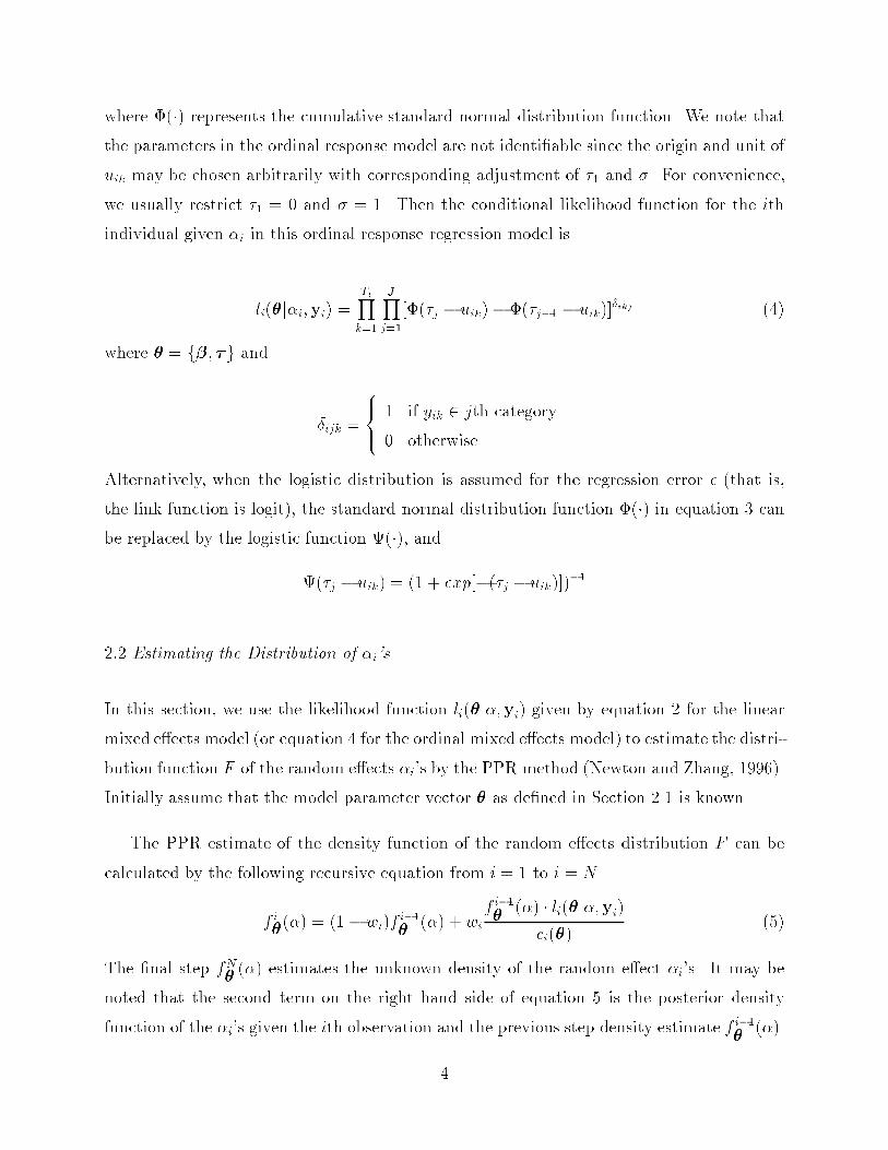
Table 1: Frequency table of Wisconsin Sleep Apnea Survey DataCategory Frequency Proportion1 1347 .222942 775 .128273 1363 .225594 717 .118675 748 .123806 1092 .18073Total 6042 1.0mated threshold parameters (with standard errors) were f�̂2 = 1:706(0:070); �̂3 = 4:232(0:122);�̂4 = 5:620(0:133); �̂5 = 7:337(0:163)g. The standard error were estimated based on 100 boot-strap data sets. The estimated regression coe�cients of sex, age and BMI were respectively1.845(0.135), 0.074(0.0084), and 0.261(0.012). Thus snoring level increases with increasingage and BMI and males tend to snore more frequently than females.Based on the ordinal regression model as described in Section 2.2, the risk score forthe ith individual falling in or above the jth category is �i + x� � �j�1. As the semi-parametric model provides estimates of �j�1, � and the distribution of �i, we can obtain theestimate of the risk score distribution at any snoring category j and �xed covariate valuesx. For example, we set j = 4 (corresponding to the risk of snoring at least once a week)and calculated the estimated risk score distribution for the subpopulation with sex=female,age=40 and BMI=26.94 (the average BMI values for females with age=40). The left panelin the following Figure 1 presents the plot of the estimated risk score density function. Wenote that this plot displays two peaks indicating that there are still two major risk groupsafter adjusting for sex, age and BMI. To further examine how the two risk groups arose, wedeleted the responses in the `Never Snore' category. The right panel is the estimated densityfunction after this exclusion. We observe that the new estimated risk score distributionis no longer bimodal. This suggests that the smaller peak arises from individuals givingthe `Never Snore' response, and that the model may not explain the di�erence betweennon-snorers and snorers very well. Alternatively, the result may indicate the existence of a12

misclassi�cation error where self-reported non-snorers may be unaware of their true status.Hence, the nonparametric �t has identi�ed several research questions for future inquiry.Based on all data

-15 -10 -5 0 5 10

Risks of snoring at least once a week

0.0

0.05

0.10

0.15

0.20

0.25

Den

sity

After excluding non-snorers

-15 -10 -5 0 5 10

Risks of snoring at least once per week

0.0

0.05

0.10

0.15

0.20

0.25

Den

sity

Figure 1: Estimated distribution densities of individual risks of snoring at least once perweek for the female subpopulation at age=40 and BMI =27. The left panel gives the densityestimate based on all collected data and the right panel gives the estimate after excludingthe `Never Snore' responses.5. DiscussionWe have proposed a semi-parametricmixed model for the analysis of longitudinal continuousor ordinal data, using the partial predictive recursion (PPR) algorithm (Newton and Zhang,1996) to estimate the distribution of the individual random e�ects. The method improvese�ciency of estimating �xed e�ects in cases of non-normally distributed random e�ects. Oursimulation studies also indicate that there is little loss of e�ciency compared to estimatorsassuming normality even when this assumption is true. Obtaining the distribution of randome�ects is often of interest in itself, as it provides insight into the distribution of populationresponse levels or risks after adjustment for known risk factors. This in turn can indicatedistributional characteristics of unknown in uential variables or, in some situations, mea-surement errors in responses. In this paper, we concentrated on the semi-parametric mixedmodel with only one random individual e�ect. The method can be extended to multiple13

random e�ects.A main advantage of our proposed method over others in the literature is its computa-tional speed. Most previous approaches used NPMLE related methods for estimating themixing distribution. The NPMLE of the mixing distribution is always discrete with a �nitenumber of mass points (Laird, 1978). When the sample size is large, however, the numberof supporting points of NPMLE can be large making NPMLE computationally burdensome.The PPR method seems more computationally convenient in estimating the mixing distri-bution for large data. Also, we greatly reduced the computation time by only estimating thedensity function of the random e�ect at the very few Gauss-Legendre quadrature abscissas.Acknowledgement:This work was supported by grants PO1 HL42242 from the National Heart Lung and BloodInstitute and R01 CA53786 from the National Cancer Institute.ReferencesBreslow, N. E. & Clayton, D. G. (1993), `Approximate inference in generalized linear mixedmodels', Journal of the American Statistical Association 88, 9{25.Carroll, R. J. & Hall, P. (1988), `Optimal rates of convergence for deconvolving a density',Journal of the American Statistical Association 83, 1184{1186.Dempster, A. P., Laird, N. M. & Rubin, D. B. (1977), `Maximum likelihood from incompletedata via the EM algorithm', Journal of the Royal Statistical Society, Series B 39, 1{38.Diciccio, T. J. & Martin, M. A. (1996), `Information bias and adjusted pro�le likelihoods',Journal of the Royal Statistical Society, Series B 58, 189{203.Follmann, D. A. & Lambert, D. (1989), `Generalizing logistics regression by nonparametricmixing', Journal of the American Statistical Association 84, 295{300.Hedeker, D. & Gibbons, R. D. (1994), `A random-e�ects ordinal regression model for multi-level analysis', Biometrics 50, 933{953.Laird, N. (1978), `Nonparametric maximum likelihood estimation of a mixing distribution',Journal of the American Statistical Association 73, 805{811.14

Laird, N. M. &Ware, J. H. (1982), `Random e�ects models for longitudinal data', Biometrics38, 963{974.Lesperance, M. L. & Kalb eisch, J. D. (1992), `An algorithm for computing the nonpara-metric MLE of a mixing distribution', Journal of the American Statistical Association87, 120{126.Lindsay, B. G. (1983), `The geometry of mixture likelihoods: A general theory', The Annalsof Statistics 11, 86{94.Magder, L. S. & Zeger, S. L. (1996), `A smooth nonparametric estimate of a mixing dis-tribution using mixtures of gaussians', Journal of the American Statistical Association91, 1141{1152.McCullagh, P. & Tibshirani, R. (1990), `A simple method for the adjustment of pro�lelikelihoods', Journal of the Royal Statistical Society, Series B 52, 325{344.Neuhaus, J. M. & Hauck, W. W. (1992), `The e�ects of mixture distribution misspeci�cationwhen �tting mixed-e�ects logistic models', Biometrika 79, 755{762.Newton, M. A. & Zhang, Y. (1996), `A partial predictive recursion', Technical Report 965,University of Wisconsin, Dept of Statistics, Madison, WI. Submitted to Biometrika.SAS (1992), SAS Technical Report P-229, SAS/STAT Software:Changes and Enhancements,Release 6.07, SAS Institute Inc.Verbeke, G. & Lesa�re, E. (1996), `A linear mixed-e�ect model with heterogeneity in therandom-e�ects population', Journal of the American Statistical Association 91, 217{221.Young, T., Palta, M. & Dempsey, J. (1993), `The occurrence of sleep-disordered breathingamong middle-aged adults', New England Journal of Medicine 328, 1230{1235.15

NORMAL Mixing Distribution

-5 0 5Alpha

0.0

0.05

0.10

0.15

0.20

0.25

0.30D

ensi

ty

EXPONENTIAL Mixing Distribution

0 5 10 15Alpha

0.0

0.1

0.2

0.3

0.4

Den

sity

BIMODAL Mixing Distribution

-2 0 2Alpha

0.0

0.5

1.0

1.5

2.0

2.5

Den

sity

NORMAL Mixing Distribution

-5 0 5Alpha

0.0

0.2

0.4

0.6

0.8

1.0

CD

F

EXPONENTIAL Mixing Distribution

0 5 10 15Alpha

0.0

0.2

0.4

0.6

0.8

1.0

CD

F

BIMODAL Mixing Distribution

-2 0 2Alpha

0.0

0.2

0.4

0.6

0.8

1.0

CD

F

NORMAL Mixing Distribution

-5 0 5Alpha

0.0

0.05

0.10

0.15

0.20

0.25

0.30

Den

sity

EXPONENTIAL Mixing Distribution

0 5 10 15Alpha

0.0

0.1

0.2

0.3

0.4

Den

sity

BIMODAL Mixing Distribution

-2 0 2Alpha

0.0

0.5

1.0

1.5

2.0

2.5D

ensi

ty

NORMAL Mixing Distribution

-5 0 5Alpha

0.0

0.2

0.4

0.6

0.8

1.0

CD

F

EXPONENTIAL Mixing Distribution

0 5 10 15Alpha

0.0

0.2

0.4

0.6

0.8

1.0

CD

F

BIMODAL Mixing Distribution

-2 0 2Alpha

0.0

0.2

0.4

0.6

0.8

1.0

CD

F Figure 2: Each plot in the �rst row contains three estimated density curves (dashed lines) aswell as the true density curves (solid lines) for one type of mixing distribution. The plots in thesecond row are the corresponding distribution functions. The plots in the two bottom rows presentthe estimated density curves and CDF's from 100 data sets for each mixing distribution. All theestimates are based on the large sample data sets N = 600.16

Table 2: Simulation ResultsMixing Dist. Model Mean(ISE) MSE(�̂1) MSE(�̂2) MSE(�̂2) �� �log(L)Small data sets(N = 50)Gaussian Gaussian .0354 .0209 .3523 .1986 { 460.06Semi-para .0532 .0222 .4346 .2030 .7581 458.37Exponential Gaussian .0825 .0211 .4263 .2211 { 458.45Semi-para .0434 .0214 .2551 .2349 .7427 452.48Bimodal Gaussian .2360 .0188 .4449 .1525 { 459.79Semi-para .1217 .0178 .1568 .2060 .5199 451.15Large data sets(N = 600)Gaussian Gaussian .0027 .0023 .0293 .0156 { 5551.8Semi-para .0049 .0024 .0312 .0159 .8385 5549.5Exponential Gaussian .0543 .0019 .0301 .0178 { 5548.0Semi-para .0071 .0019 .0207 .0191 .8046 5475.9Bimodal Gaussian .2070 .0017 .0445 .0184 { 5552.7Semi-para .0486 .0016 .0110 .0218 .5034 5450.7Table 3: The simulation results compared with the other methodsMixing Dist. Method Mean(ISE) MSE(�̂1) MSE(�̂2)Moderate Sample Size(N = 180)Gaussian Gaussian� .0099 .0107 .1281NPMLE� .0776 .0107 .1759SNPMLE� .0166 .0107 .1421PPR .0157 .0107 .1397Skewed Gaussian� .0580 .0109 .1356NPMLE� .0759 .0107 .1142SNPMLE� .0184 .0106 .0988PPR .0195 .0105 .0880Bimodal Gaussian� .2145 .0083 .1211NPMLE� .0877 .0076 .0439SNPMLE� .1326 .0079 .0557PPR .0814 .0076 .0505*: These are from table 3 of the paper by Mager and Zeger (1996).17