Shear Wind Estimation

Ricardo Bencatel∗, Joao Sousa †

School of Engineering, University of Porto, Porto, 4200, Portugal

Mariam Faied‡ and Anouck Girard§

University of Michigan, Ann Arbor, Michigan, MI 48109, USA

This paper presents atmospheric Shear Wind phenomena models and develops a Parti-cle Filter estimator to characterize the phenomena. We describe a model for the SurfaceShear Wind and another for the Layer Shear Wind. The models are described and ad-justed for Besian estimation. A Particle Filter was implemented and tested in simulationfor Surface Shear Wind parameter estimation. The estimator was idealized to be usedby small Unmanned Aerial Vehicles (UAVs). The implemented Particle Filter estimatesthe surrounding flow field with a small number of variables, and as such, low memoryrequirements.

Nomenclature

[x, y, z] Position vectorhSSW,ref Surface Shear Wind gradient reference altitudeWSSW,ref Surface Shear Wind reference speedψSSW Surface Shear Wind main directionhSSW,0 Surface Shear Wind roughness altitude

hLSW Layer Shear Wind mean altitude∆hLSW Layer Shear Wind heightwLSW Layer Shear Wind reference velocity∆wLSW Layer Shear Wind velocity variation

I. Introduction

Small Unmanned Aerial Vehicles (UAVs) are becoming a reference tool by field operatives that needto enhance their situational awareness. However, the desired small size brings together the consequence ofreduced energy capacity, either in fuel or battery power. A solution for this problem is to increase theirendurance by harvesting energy from atmospheric phenomena.

Shear Wind is the atmospheric phenomenon which occurs on thin layers separating two regions wherethe predominant air flow vector is different. This difference can be either in speed, in direction, or in bothspeed and direction. The air layer between these regions is usually less than 100 meters thick, originating apersistent gradient in the flow field. This gradient may be exploited by UAVs?,?,?,? as it is by birds.?,?

The Shear Wind phenomena can be classified by directionality as Vertical or Horizontal Shear. VerticalShear Wind is a variation of the air flow with altitude. It exists near the ground or water surface,?, ? on theinversion layer, and on the limits of the jet stream.? Surface wind shear is known on the aviation communitymainly by its effects on aircraft landing and take-off operations. The reduction of flow speed towards theground causes the aircraft airspeed to decrease in the same amount, if no compensation is applied. Thiseffect can induce stall, leading to possible catastrophic results. Glider pilots observe Shear Wind sometimes

∗PhD student, Department of Electrical and Computer Engineering†Invited assistant, Department of Electrical and Computer Engineering‡Post-doc researcher, Department of Aerospace Engineering, 1320 Beal Ave, and AIAA Member§Assistant Professor, Department of Aerospace Engineering, 1320 Beal Ave, and AIAA Life Member

1 of 8

American Institute of Aeronautics and Astronautics

above 3 knots per 1000 feet.? Horizontal Shear Wind is a variation of the air flow with a variation with thehorizontal position [x, y]. It appears across weather fronts and near the coast.

In this work the flow field is the spatial characterization of the air velocity vector. Further, we will referto the flow field horizontal velocity vector as the wind vector.

I.A. Literature review

The problem of harvesting energy from atmospheric phenomena was addressed by some authors regardingupdrafts, Shear Wind and gusts. Allen? describes an updraft phenomenon, known as thermals, which isused by glider pilots to remain aloft without a propulsion system. Edwards? proved that thermal soaringis feasible with UAVs. He achieved long flights, both in time and flown distance, at several different flightsites. Langelaan? describes how gusts affect aircraft and how flight controllers can lead the aircraft to looseor gain energy with gusts. Lawrance and Sukkarieh?, ?, ? presented energy based methods for soaring pathplanning. The first work describes a method suitable for static and dynamic soaring, i.e., both in thermalsand shear flow fields. The second work describes a promising controller for Shear Wind soaring. The thirdwork describes a path planner to simultaneously acquire information about the surrounding flow field andexplore the available flow energy. Sachs? describes how birds and aircraft can harvest energy from surfaceShear Wind. He also determines the bound conditions for perpetual flight with this phenomenon. Sachs etal.? studied Albatross real flight paths while these were take advantage of the Surface Shear Wind.

I.B. General problem

As described before, energy harvest from Shear Wind phenomena should be feasible. We will focus onVertical Shear Wind, as surface, inversion, and jet stream shear are quite steady phenomena. Birds learnhow to use these phenomena. UAVs may be programmed to do the same. The main requirements are:knowing the phenomenon characteristics and control the aircraft to execute an energy harvesting flight path.The control methods developed by Lawrance and Sukkarieh?, ?, ? required knowledge of the surrounding flowfield. These phenomena occur over large areas, which makes it difficult to characterize as a whole. Lawranceand Sukkarieh’s solution for this characterization is a Gaussian Progress (GP) regression that describes theflow field over spatially distributed points.

I.C. Current approach

Our approach is a model-based estimation, requiring few characterization parameters. As such, we simplifythe phenomena to uniaxial (z) wind vector variations, i.e., define the wind vector as a function of the altitudeonly. We further distinguish the Vertical Shear Wind phenomena in Surface and Layer Shear Wind, as theflow gradient is different for each phenomena. We will describe both phenomena modelling functions andthe sensing method in section II.

To estimate the characterizing parameters we developed a Particle Filter. Particle Filters handle wellthe phenomena nonlinearities and may be extended to simultaneously localize several different Shear Windlayers. In section III we define the propagation and observation models and estimations method.

The results and conclusions are described in sections IV and V.

II. Models

II.A. Surface Shear Wind

Surface Shear Wind is a special case of vertical shear where instead of two air mass regions we have oneair mass region and a surface. The surface is usually still or moving at very low speeds relatively to thegeneral air mass, as is the case of water surfaces. The Shear Wind layer starts at the ground level and maybe modeled by:?,?

WH = WHref

ln (h/h0)

ln (href/h0), (1)

where WH is the total wind speed and WHref, href , and h0 are reference values. WHref

is the reference windspeed at an altitude href away from the surface. h0 defines the shape of the flow gradient, reflecting the

2 of 8

American Institute of Aeronautics and Astronautics

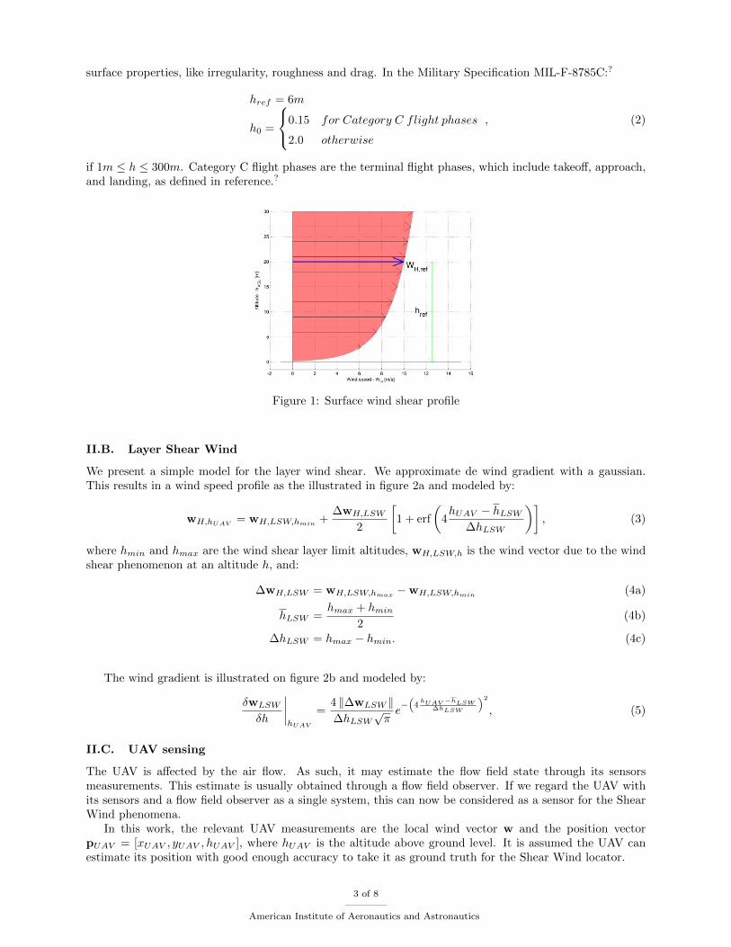
surface properties, like irregularity, roughness and drag. In the Military Specification MIL-F-8785C:?

href = 6m

h0 =

0.15 for Category C flight phases

2.0 otherwise

, (2)

if 1m ≤ h ≤ 300m. Category C flight phases are the terminal flight phases, which include takeoff, approach,and landing, as defined in reference.?

Figure 1: Surface wind shear profile

II.B. Layer Shear Wind

We present a simple model for the layer wind shear. We approximate de wind gradient with a gaussian.This results in a wind speed profile as the illustrated in figure 2a and modeled by:

wH,hUAV= wH,LSW,hmin

+∆wH,LSW

2

[1 + erf

(4hUAV − hLSW

∆hLSW

)], (3)

where hmin and hmax are the wind shear layer limit altitudes, wH,LSW,h is the wind vector due to the windshear phenomenon at an altitude h, and:

∆wH,LSW = wH,LSW,hmax−wH,LSW,hmin

(4a)

hLSW =hmax + hmin

2(4b)

∆hLSW = hmax − hmin. (4c)

The wind gradient is illustrated on figure 2b and modeled by:

δwLSW

δh

∣∣∣∣hUAV

=4 ‖∆wLSW ‖∆hLSW

√πe−(

4hUAV −hLSW

∆hLSW

)2

, (5)

II.C. UAV sensing

The UAV is affected by the air flow. As such, it may estimate the flow field state through its sensorsmeasurements. This estimate is usually obtained through a flow field observer. If we regard the UAV withits sensors and a flow field observer as a single system, this can now be considered as a sensor for the ShearWind phenomena.

In this work, the relevant UAV measurements are the local wind vector w and the position vectorpUAV = [xUAV , yUAV , hUAV ], where hUAV is the altitude above ground level. It is assumed the UAV canestimate its position with good enough accuracy to take it as ground truth for the Shear Wind locator.

3 of 8

American Institute of Aeronautics and Astronautics

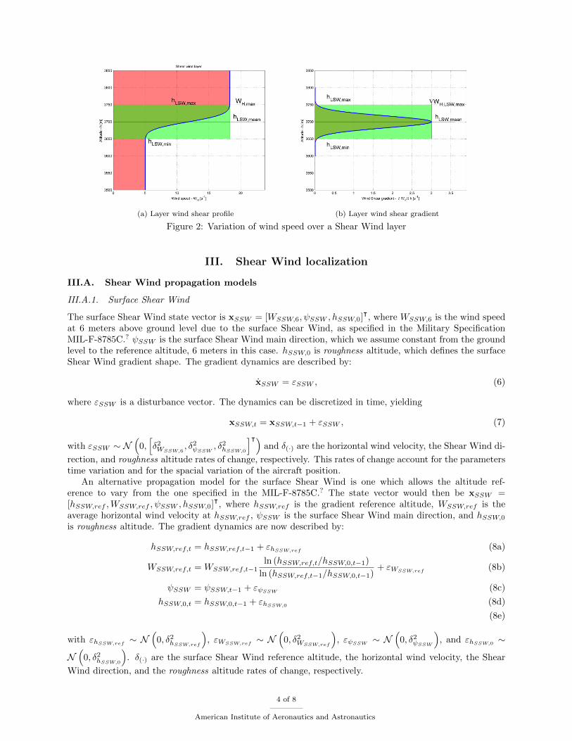
(a) Layer wind shear profile (b) Layer wind shear gradient

Figure 2: Variation of wind speed over a Shear Wind layer

III. Shear Wind localization

III.A. Shear Wind propagation models

III.A.1. Surface Shear Wind

The surface Shear Wind state vector is xSSW = [WSSW,6, ψSSW , hSSW,0]ᵀ, where WSSW,6 is the wind speed

at 6 meters above ground level due to the surface Shear Wind, as specified in the Military SpecificationMIL-F-8785C.? ψSSW is the surface Shear Wind main direction, which we assume constant from the groundlevel to the reference altitude, 6 meters in this case. hSSW,0 is roughness altitude, which defines the surfaceShear Wind gradient shape. The gradient dynamics are described by:

xSSW = εSSW , (6)

where εSSW is a disturbance vector. The dynamics can be discretized in time, yielding

xSSW,t = xSSW,t−1 + εSSW , (7)

with εSSW ∼ N(

0,[δ2WSSW,6

, δ2ψSSW

, δ2hSSW,0

]ᵀ)and δ(·) are the horizontal wind velocity, the Shear Wind di-

rection, and roughness altitude rates of change, respectively. This rates of change account for the parameterstime variation and for the spacial variation of the aircraft position.

An alternative propagation model for the surface Shear Wind is one which allows the altitude ref-erence to vary from the one specified in the MIL-F-8785C.? The state vector would then be xSSW =[hSSW,ref ,WSSW,ref , ψSSW , hSSW,0]

ᵀ, where hSSW,ref is the gradient reference altitude, WSSW,ref is the

average horizontal wind velocity at hSSW,ref , ψSSW is the surface Shear Wind main direction, and hSSW,0is roughness altitude. The gradient dynamics are now described by:

hSSW,ref,t = hSSW,ref,t−1 + εhSSW,ref(8a)

WSSW,ref,t = WSSW,ref,t−1ln (hSSW,ref,t/hSSW,0,t−1)

ln (hSSW,ref,t−1/hSSW,0,t−1)+ εWSSW,ref

(8b)

ψSSW = ψSSW,t−1 + εψSSW(8c)

hSSW,0,t = hSSW,0,t−1 + εhSSW,0(8d)

(8e)

with εhSSW,ref∼ N

(0, δ2

hSSW,ref

), εWSSW,ref

∼ N(

0, δ2WSSW,ref

), εψSSW

∼ N(

0, δ2ψSSW

), and εhSSW,0

∼

N(

0, δ2hSSW,0

). δ(·) are the surface Shear Wind reference altitude, the horizontal wind velocity, the Shear

Wind direction, and the roughness altitude rates of change, respectively.

4 of 8

American Institute of Aeronautics and Astronautics

III.A.2. Layer Shear Wind

The layer Shear Wind state vector is xLSW =[hLSW ,∆hLSW ,wLSW ,∆wLSW

]ᵀ, where hLSW is the mean

altitude of the Shear Wind layer, ∆hLSW is Shear Wind layer height, wLSW and ∆wLSW are the horizontalwind vector mean and variation over the Shear Wind layer. As with the surface Shear Wind, this is only acorrect representation of the layer Shear Wind if we assume a constant wind gradient direction. The gradientdynamics are described by:

xLSW = εLSW , (9)

where εLSW is a disturbance vector. The dynamics can be discretized in time, yielding

xLSW,t = xLSW,t−1 + εLSW , (10)

with εLSW ∼ N(

0,[δ2hLSW

, δ2∆hLSW

, δ2µW,LSW

ᵀ, δ2

∆WLSW

ᵀ]ᵀ)

and δ(·) are the rates of change of the all layer

Shear Wind state parameters, respectively. As with the surface Shear Wind parameters, this rates of changeaccount for the parameters time variation and the change with spacial variation of the aircraft position.

III.B. Shear Wind observation models

The horizontal wind vector observation (wH) may be described by

wH = [Wx,Wy]ᵀ ≈ h (xSW ,pUAV ) + εWH

, (11)

where Wx and Wy are estimated with a wind observer.The observation uncertainty (εWH

) is caused mainly by gusts, but also by the UAV sensing noise, i.e.,the wind observer errors. As such, it may be defined as:

εWH= εWH ,Gust + εWH ,Sens (12a)

εWH ,Gust ∼ N(0, kGust · wH

)(12b)

εWH ,Sens ∼ N (0, σWObs) , (12c)

where kGust is an adimensional ratio relating the wind variation with the wind average:

kGust =

√E

[(‖wH‖ − ‖wH‖

)2]

‖wH‖, (13)

wH is the estimate of the average horizontal wind, and σWObs is the wind observer uncertainty vector.

III.B.1. Surface Shear Wind

The surface Shear Wind observation model is derived from (1):

wH = h (xSSW ,pUAV ) = WSSW,refln (hUAV /hSSW,0)

ln (hSSW,ref/hSSW,0)

[cosψSSW

sinψSSW

]. (14)

III.B.2. Layer shear

The layer Shear Wind observation model is derived from (3):

wH = h (xLSW ,pUAV ) = whmin,LSW +∆wLSW

2

[1 + erf

(4hUAV − hLSW

∆hLSW

)], (15)

where whmin,LSW = wLSW − ∆wLSW

2 .

5 of 8

American Institute of Aeronautics and Astronautics

III.C. Inference framework

In this work, the estimation is implemented through a Particle Filter. The belief distribution at eachestimation step is represented by particles defined by the state vector xSSW or xLSW . Each particle is anhypothesis of the current state. At each step, particles are propagated, evaluated and resampled, to createa new estimate. The particles are propagated through the propagation model described in section III.A.This step allows the filter to track the state evolution and represent the uncertainty. The observation model,presented in section III.B, generates the expected observation for each particle. This is combined with theUAV observation to provide a measurement of likelihood of the hypothesis represented by each particle. Theresampling prunes the unlikely particles (hypothesis).

III.D. Particle generation

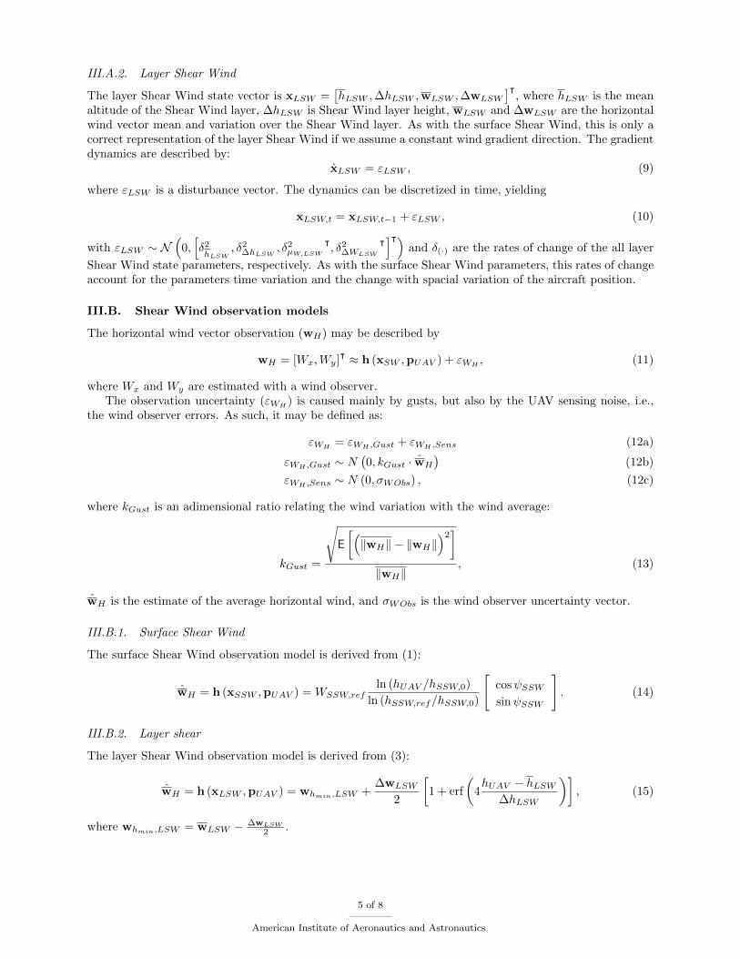
Figure 3: Surface Shear Wind ”roughness” altitude distribution generated

III.D.1. Surface Shear Wind

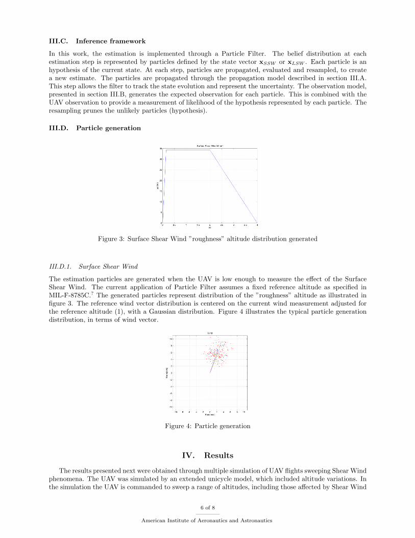
The estimation particles are generated when the UAV is low enough to measure the effect of the SurfaceShear Wind. The current application of Particle Filter assumes a fixed reference altitude as specified inMIL-F-8785C.? The generated particles represent distribution of the ”roughness” altitude as illustrated infigure 3. The reference wind vector distribution is centered on the current wind measurement adjusted forthe reference altitude (1), with a Gaussian distribution. Figure 4 illustrates the typical particle generationdistribution, in terms of wind vector.

Figure 4: Particle generation

IV. Results

The results presented next were obtained through multiple simulation of UAV flights sweeping Shear Windphenomena. The UAV was simulated by an extended unicycle model, which included altitude variations. Inthe simulation the UAV is commanded to sweep a range of altitudes, including those affected by Shear Wind

6 of 8

American Institute of Aeronautics and Astronautics

phenomena. The wind simulation summed the Shear Wind effects to gusts. The gusts were generated by ascalar Gauss-Markov process, which simulates well the kind of sensing noise the system would be subject toin reality.

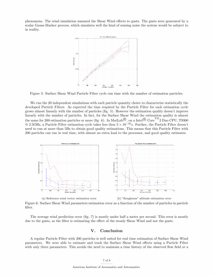
Figure 5: Surface Shear Wind Particle Filter cycle run time with the number of estimation particles.

We run the 20 independent simulations with each particle quantity choice to characterize statistically thedeveloped Particle Filters. As expected the time required by the Particle Filter for each estimation cyclegrows almost linearly with the number of particles (fig. 5). However the estimation quality doesn’t improvelinearly with the number of particles. In fact, for the Surface Shear Wind the estimation quality is almost

the same for 200 estimation particles or more (fig. 6). In MatLab R©, on a Intel R© CoreTM

2 Duo CPU, T9300@ 2.5GHz, a Particle Filter estimation cycle takes less then 5× 10−30s. Further, the Particle Filter doesn’tneed to run at more than 5Hz to obtain good quality estimations. This means that this Particle Filter with200 particles can run in real time, with almost no extra load to the processor, and good quality estimates.

(a) Reference wind vector estimation error (b) ”Roughness” altitude estimation error

Figure 6: Surface Shear Wind parameters estimation error as a function of the number of particles in particlefilter.

The average wind prediction error (fig. 7) is mostly under half a meter per second. This error is mostlydue to the gusts, as the filter is estimating the effect of the steady Shear Wind and not the gusts.

V. Conclusion

A regular Particle Filter with 200 particles is well suited for real time estimation of Surface Shear Windparameters. We were able to estimate and track the Surface Shear Wind effects using a Particle Filterwith only three parameters. This avoids the need to maintain a time history of the observed flow field or a

7 of 8

American Institute of Aeronautics and Astronautics

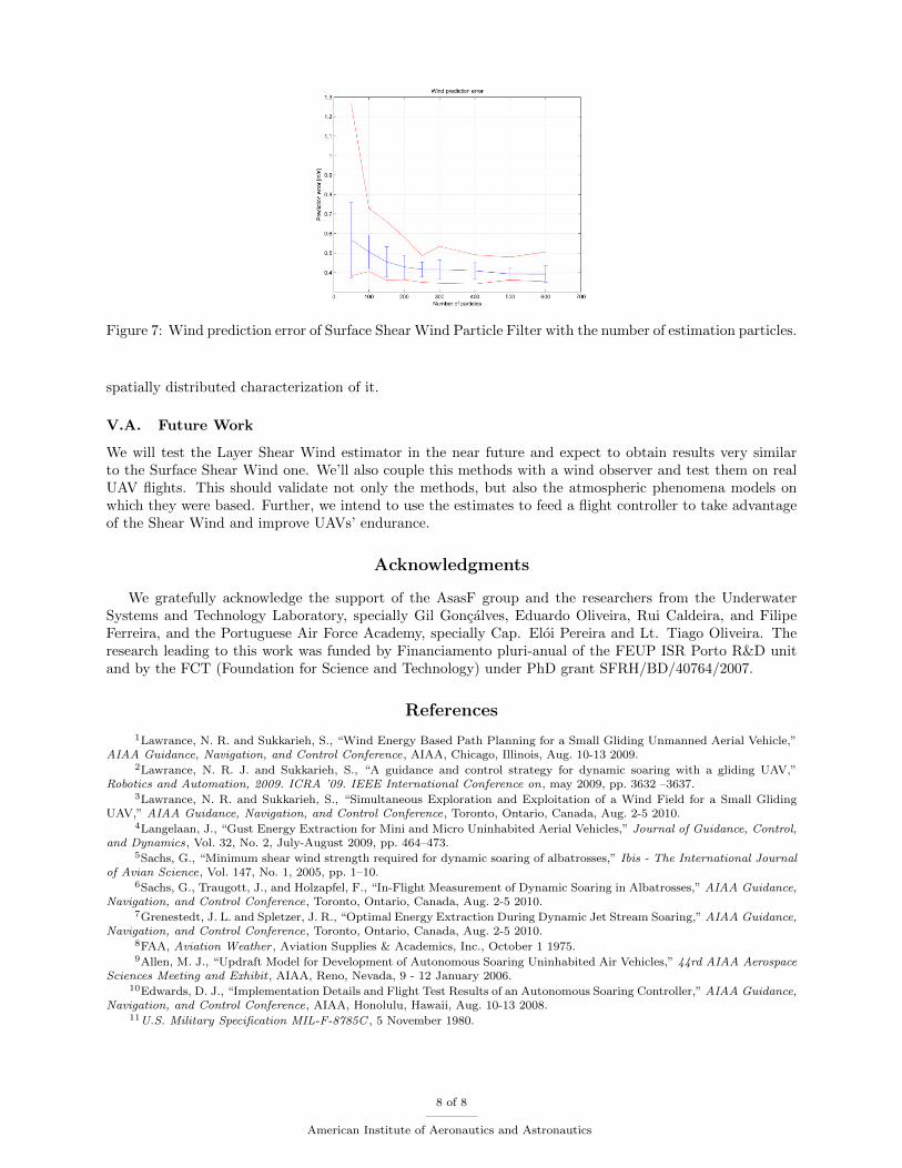
Figure 7: Wind prediction error of Surface Shear Wind Particle Filter with the number of estimation particles.

spatially distributed characterization of it.

V.A. Future Work

We will test the Layer Shear Wind estimator in the near future and expect to obtain results very similarto the Surface Shear Wind one. We’ll also couple this methods with a wind observer and test them on realUAV flights. This should validate not only the methods, but also the atmospheric phenomena models onwhich they were based. Further, we intend to use the estimates to feed a flight controller to take advantageof the Shear Wind and improve UAVs’ endurance.

Acknowledgments

We gratefully acknowledge the support of the AsasF group and the researchers from the UnderwaterSystems and Technology Laboratory, specially Gil Goncalves, Eduardo Oliveira, Rui Caldeira, and FilipeFerreira, and the Portuguese Air Force Academy, specially Cap. Eloi Pereira and Lt. Tiago Oliveira. Theresearch leading to this work was funded by Financiamento pluri-anual of the FEUP ISR Porto R&D unitand by the FCT (Foundation for Science and Technology) under PhD grant SFRH/BD/40764/2007.

References

1Lawrance, N. R. and Sukkarieh, S., “Wind Energy Based Path Planning for a Small Gliding Unmanned Aerial Vehicle,”AIAA Guidance, Navigation, and Control Conference, AIAA, Chicago, Illinois, Aug. 10-13 2009.

2Lawrance, N. R. J. and Sukkarieh, S., “A guidance and control strategy for dynamic soaring with a gliding UAV,”Robotics and Automation, 2009. ICRA ’09. IEEE International Conference on, may 2009, pp. 3632 –3637.

3Lawrance, N. R. and Sukkarieh, S., “Simultaneous Exploration and Exploitation of a Wind Field for a Small GlidingUAV,” AIAA Guidance, Navigation, and Control Conference, Toronto, Ontario, Canada, Aug. 2-5 2010.

4Langelaan, J., “Gust Energy Extraction for Mini and Micro Uninhabited Aerial Vehicles,” Journal of Guidance, Control,and Dynamics, Vol. 32, No. 2, July-August 2009, pp. 464–473.

5Sachs, G., “Minimum shear wind strength required for dynamic soaring of albatrosses,” Ibis - The International Journalof Avian Science, Vol. 147, No. 1, 2005, pp. 1–10.

6Sachs, G., Traugott, J., and Holzapfel, F., “In-Flight Measurement of Dynamic Soaring in Albatrosses,” AIAA Guidance,Navigation, and Control Conference, Toronto, Ontario, Canada, Aug. 2-5 2010.

7Grenestedt, J. L. and Spletzer, J. R., “Optimal Energy Extraction During Dynamic Jet Stream Soaring,” AIAA Guidance,Navigation, and Control Conference, Toronto, Ontario, Canada, Aug. 2-5 2010.

8FAA, Aviation Weather , Aviation Supplies & Academics, Inc., October 1 1975.9Allen, M. J., “Updraft Model for Development of Autonomous Soaring Uninhabited Air Vehicles,” 44rd AIAA Aerospace

Sciences Meeting and Exhibit , AIAA, Reno, Nevada, 9 - 12 January 2006.10Edwards, D. J., “Implementation Details and Flight Test Results of an Autonomous Soaring Controller,” AIAA Guidance,

Navigation, and Control Conference, AIAA, Honolulu, Hawaii, Aug. 10-13 2008.11U.S. Military Specification MIL-F-8785C , 5 November 1980.

8 of 8

American Institute of Aeronautics and Astronautics