Wind-shear induced stabilization of PCI

1212 J. Opt. Soc. Am. A/Vol. 15, No. 5 /May 1998 D. L. Fried and R. K.-H. Szeto

Wind-shear induced stabilization of PCI

David L. Fried

151 Bernal Road, Suite 2, San Jose, California 95119-1306

Roque Kwok-Hung Szeto

Earth Resources Laboratory, Massachusetts Institute of Technology, 42 Carleton Street, Cambridge,Massachusetts 02142-1324

Received April 22, 1997; revised manuscript received November 24, 1997; accepted November 24, 1997

Phase compensation instability (PCI) is a runaway process associated with the operation of a closed-loopphase-only adaptive-optics system transmitting through the atmosphere a large-diameter laser beam with ahigh power density. Under most conditions such an operation introduces positive feedback; if the laser powerdensity is sufficiently high, there is the possibility of PCI-type runaway of the adaptive-optics servo. It is nowknown that the occurrence of PCI is inhibited by wind shear (wind-shear induced stabilization of PCI, orWISP) because at every different position along the propagation path the turbulent wind has a (slightly) dif-ferent component of velocity in the plane transverse to the laser beam’s propagation direction. We develop aset of equations from which the conditions for the onset of PCI can be determined. Sample results are pre-sented for propagation through an atmosphere with a negative exponential absorption profile—which nomi-nally corresponds to ground-to-space propagation. The results indicate that for typical conditions (as a con-sequence of wind shear) one can transmit a rather substantial laser power density without encountering PCI.As an example of the application of our theory, the expected Strehl ratio for a HV5/7 turbulence model is evalu-ated for the parameters of a nominal ground-to-space high-energy laser beam propagation system. © 1998Optical Society of America [S0740-3232(98)01105-3]

OCIS codes: 350.5030, 010.1080, 010.1300, 120.6810.

1. INTRODUCTION AND OVERVIEWPhase compensation instability (PCI) is a runaway pro-cess associated with the operation of a closed-loop phase-only adaptive-optics system transmitting through the at-mosphere a large-diameter laser beam with a high powerdensity.1–4 The PCI process depends on (1) the conver-sion, by propagation, of high-spatial-frequency phase per-turbations of the transmitted laser beam into correspond-ing spatial-frequency intensity perturbations of that laserbeam; (2) the perturbation of the atmosphere’s tempera-ture or refractive index by the absorption of the laserbeam’s intensity perturbations; (3) the effect of therefractive-index perturbations on the beacon referencesource (which is sensed by the adaptive optics system);and finally (4) the imposition by the adaptive-optics sys-tem of additional phase perturbations on the transmittedlaser beam in response to the phase perturbations of thebeacon. Under conditions of interest this is a positive-feedback situation with the possibility of PCI runaway ofthe adaptive-optics servo.

The adaptive-optics system of the laser transmitter hasthe ability to sense (in the beacon) and compensate (forthe transmitted laser beam) the relatively high-spatial-frequency components of the phase–wave-front distortioninduced by atmospheric turbulence. Such atmosphericturbulence effects unavoidably serve as a seed for the PCIprocess.

It is known from experiment5 that the occurrence ofPCI is inhibited by wind shear, i.e., because at every dif-ferent position along the propagation path the component

0740-3232/98/051212-15$15.00 ©

of the turbulent wind in the plane transverse to the laserbeam’s propagation direction has a (slightly) different ve-locity. To see why wind shear might be expected to in-hibit the occurrence of PCI, we consider that when arefractive-index variation is induced at some instant by aperturbation in the laser beam’s intensity, the samevariation is induced in many or all of the slabs of atmo-sphere that together make up the propagation path. Be-cause initially the refractive-index variations along thepropagation path are all equivalent (i.e., they are allaligned with one another relative to the propagation di-rection), the phase perturbations induced in the beaconby the refractive-index variation in each of these slabs allcombine coherently; they combine in such a way as tomake the induced phase perturbation as large as possible.This, however, is true only initially. At subsequent timeswind shear causes the various slabs to be displaced differ-ent amounts, and as a consequence the phase perturba-tions of the beacon that are induced by each of the slabscombine in a less coherent way. The net effect is a reduc-tion in the significance of the atmospheric heating orrefractive-index perturbation that took place previously;the greater the age of the refractive-index perturbation,the less significant its current effect. It can be shownthat the extent of the aging depends on the wind-shearvelocity spread and on the spatial frequency of the pertur-bation.

It should be recognized that wind shear has nothing todo with a reduction in the heating or temperature orrefractive-index perturbations that occur with increasing

1998 Optical Society of America

D. L. Fried and R. K.-H. Szeto Vol. 15, No. 5 /May 1998/J. Opt. Soc. Am. A 1213

time but simply follows from the loss of alignment be-tween the slabs of the perturbation pattern.6 The effectof wind shear is distinct from the effect of turbulent mix-ing, which reduces the magnitude of the perturbationsbut can be seen to be a much slower process (and is nottreated in this paper).

If we assume that the laser beam adaptive-optics aper-ture diameter is large, then the occurrence of PCI de-pends only on the laser power density, the atmosphericabsorption coefficient, the wind-shear spread in trans-verse wind velocity, and the highest spatial-frequencycorrection or perturbation that the adaptive optics is de-signed to be able to impose on the transmitted laserbeam. [The laser beam diameter can be considered largeif the wind-clearing time (i.e., the diameter divided by theeffective average wind speed) is many times the misalign-ment time (which may be considered equal to the wave-length associated with the relevant spatial frequency di-vided by the effective rms wind shear, i.e., the rms spreadin wind velocity)].

In this paper we develop a theory for the effect of windshear on the PCI process, study these matters, and derivean understanding of the quantitative aspects of the pro-cess governing the onset of PCI. In particular, we shallobtain results allowing us to determine the laser powerdensity below which PCI does not occur. Our approachto determining the laser power density for the onset ofPCI is based on the use of perturbation theory for analy-sis of optical propagation. We argue that if the resultswe obtain do not grow in an unbounded way, thus indi-cating that the conditions do not satisfy the requirementsfor the onset of PCI, then perturbation results can be re-lied on, and the time-dependent solutions will attain asteady-state form. If, on the other hand, we find that theresults do grow with time in an unbounded way, then (un-less some nonlinear ameliorating process—which we donot have any reason to believe is present—is operative)clearly the conditions satisfy the requirements for the on-set of PCI, even though we cannot use the perturbationresults per se.

The use of perturbation theory always raises an uncer-tainty as to the range of validity or accuracy of the resultsobtained. To address this we simply note that the em-phasis of our work is to establish the fact that (random)wind shear will suppress PCI and to determine the condi-tion (i.e. the propagation or physical parameters) underwhich PCI will be present despite the wind shear. Ourprincipal concern is whether or not the perturbationgrows exponentially or approaches a limit. In the formercase, the rate of exponential divergence is of no real con-cern. What matters is that in this case there is exponen-tial growth; our quantitative interest is limited to thevalue of the propagation or physical parameters for whichPCI is not suppressed. In the latter case, when the levelof perturbation reaches a finite limit, that limiting valueis of some small interest, but what is of fundamental un-derlying interest is the fact that for those propagation orphysical parameters PCI is suppressed. To the extentthat one questions the accuracy of the perturbation treat-ment, one questions the accuracy of the limiting level ofthe perturbation and not the suppression of PCI. Such aquestion is really one of the magnitude of the contribution

of higher-order terms due to nonlinearities, whether ornot they might be comparable to the first-order (linear)terms—but this is clearly a secondary matter relative tothe principal question of whether or not there is exponen-tial growth. Accordingly, we feel quite comfortable withthe use of a perturbation analysis since we are basicallyasking only whether the perturbation is contained orgrows exponentially, with only a secondary concern as toexactly what the level of containment is.

It is perhaps worth noting that if there is no PCI thenthe results are nominally in the domain of perturbationand the results are nominally reliable. A key observa-tion here is that when the perturbation is contained, i.e.,when there is no PCI, the calculated level of perturbationreached is proportional to the initial (atmospheric turbu-lence provided) seed for the physical process. In consid-ering this we offer the heuristic notion that we have beenunable to conceive of any process in which nonlinearitiesin the thermal or adaptive-optics propagation processcould circumvent the suppression of perturbation by windshear—if the wind shear were sufficient to suppress thegrowth starting from an initial turbulence seed present inthe atmosphere, then it would be just as effective with thenonlinearities present.

Of course, in discussing the accuracy of a perturbationanalysis, we can fully resolve the matter of limits of accu-racy only by recourse to experimental results. In Section5 we briefly note some experimental work5 that appearsto validate the perturbation results we develop in thiswork.

Our perturbation analysis is based on a spatial-frequency decomposition of the perturbed high-energy la-ser beam, of the beacon, of the laser-heating-inducedrefractive-index pattern, and of the naturally occurringrefractive-index turbulence pattern. Starting from theparaxial equations derived from Maxwell’s wave equa-tion, we obtain a set of differential equations involvingonly a single spatial frequency. (Because of the pertur-bation nature of the analysis there is no cross coupling be-tween different spatial-frequency components. This iswhat makes it possible to obtain equations involving onlycomponents for a single spatial frequency.) These differ-ential equations involve only two independent variables,time and position, along the propagation path.

The differential equations are inhomogeneous, showinga dependence on a continuous distribution of turbulencealong the propagation path. The refractive-index turbu-lence function appearing in these differential equationsrelates to a single spatial-frequency component. We in-voke Taylor’s frozen turbulence assumption, which allowsthe time dependence to be represented by a ‘‘frozen’’ (i.e.,unchanging) turbulence pattern and a frozen heating pat-tern, which are shifted by the transverse wind shear.

The linear nature of the differential equations makes itpossible to cast them in a Green’s function form, thus re-placing the continuous turbulence function with a deltafunction of unit strength, corresponding to refractive-index turbulence (for the spatial frequency of interest) oc-curring at some single position along the propagationpath. This delta function (turbulence representation)serves as a seed for the process in which wind shear in-teracts with the effect associated with PCI: wind-shear


induced stabilization of PCI (WISP). We refer to thesedifferential equations as the time-dependent WISP equa-tions.

In Section 2 we develop these equations. Numericalmethods for the solutions of the time-dependent WISPdifferential equations are discussed in Section 3. A novelapproach is given to model the wind-shear physics accu-rately.

Some sample results are presented in Section 4. It isfound that the time-dependent solution does approach asteady-state result if the laser power density is not toohigh. If the laser power is excessive, then it is found thatthe time-dependent solution shows exponentialgrowth—a clear manifestation of the runaway process re-ferred to as PCI.

In examining the time-dependent results, we note aninteresting feature regarding the apparent translation ofthe solution. When there is no PCI, the steady-state so-lution is seen to move at the same velocity as the turbu-lent transverse wind velocity, i.e., the wind-shear velocityfor the position along the propagation path where thedelta function unit strength refractive-index turbulenceseed is positioned. The steady-state pattern follows themotion of the turbulence seed. However, when PCI oc-curs, the time dependence is found not only to grow expo-nentially but also, after a rather short while, to move, ap-parently, at some well-defined velocity that generally isdistinctly different from the velocity of the turbulenceseed. When PCI occurs, the pattern moves indepen-dently of its original source or seed; we may concludethat it is independent of its seed. The refractive-indexturbulence that served as the seed has no effect on therunaway process once it is started. We might say thatonce PCI starts, the turbulence thermal-blooming interac-tion that seeded the process becomes irrelevant.

When PCI occurs, we see that the time-dependent so-lution grows without limit. On the other hand, whenconditions do not allow the occurrence of PCI, we see thatthe solution reaches a steady state. In Section 5 we ex-ploit this insight to derive the steady-state equations gov-erning the WISP process. From these equations we ob-tain a very simple result establishing the conditions forPCI to occur—a set of equations corresponding to thesteady-state solution with an infinite value. These equa-tions are solved to determine (in normalized form) the la-ser power density at which PCI occurs. (This laser powerdensity is a function of the spatial frequency at which thephase-only adaptive optics operates.) A comparison ofthese results (for the laser power density associated withthe onset of PCI) with those results developed in Sections2 and 3 by use of the time-dependent formulation showsgood agreement as to the threshold of the laser powerdensity for the occurrence of PCI.

The Strehl ratio for a particular turbulence model isevaluated in Section 6. Our investigations appear to in-dicate that the atmosphere under typical conditions cansupport PCI-free high-energy laser beam propagationwith good system performance.

2. TIME-DEPENDENT PROBLEMA perturbed upward-propagating high-energy laser(HEL) beam UHEL(r, s, t) and a perturbed downward-

propagating beacon beam Ubeacon(r, s, t) can be repre-sented by the equations

UHEL~r, s, t ! 5 U↑~r, s, t !exp@2pi~ ks 2 ft !#, (1)

Ubeacon~r, s, t ! 5 U↓~r, s, t !exp@22pi~ ks 1 ft !#.(2)

In Eqs. (1) and (2), U↑(r, s, t) and U↓(r, s, t) are theslowly varying parts of their respective optical fields andrepresent perturbations from a constant value that maybe considered to correspond to a perfect infinite planewave. The notation t denotes time, s denotes the posi-tion along the propagation path (with s 5 0 correspond-ing to the transmitter aperture plane), and r denotes atwo-component position vector, with components (x, y),defining the position in a plane perpendicular to thepropagation path. The notation f denotes the optical fre-quency (f 5 c/l), and k denotes the optical wave number(k 5 l21). Using the paraxial approximation in whichU↑(r, s, t) and U↓(r, s, t) change very slowly along thepropagation direction as compared with the rate at whichthey change along the transverse direction, and also us-ing the small perturbation approximation in which therefractive-index variation quadratic term @n(r, s, t)#2

can be neglected, we can obtain the paraxial small-perturbation-propagation equations for the upward HELbeam and for the downward beacon beam—namely

]sU↑~r, s, t ! 2

12 ik21¹'

2 U↑~r, s, t !

2 ikn~r, s, t !U↑~r, s, t ! 5 0, (3)

]sU↓~r, s, t ! 1

12 ik21¹'

2 U↓~r, s, t !

1 ikn~r, s, t !U↓~r, s, t ! 5 0. (4)

We are using the notation ]s [ ]/]s and ¹'2 [ ]2/]x2

1 ]2/]y2.To separately take account of the different physics of

the two distinct contributions to the total refractive-indexvariation n(r, s, t), we introduce separate functions forthe initially present atmospheric-turbulence contributionto the refractive index, denoted nT (r, s, t), and for therefractive-index perturbation due to HEL heating of theatmosphere along the propagation path, denotednH (r, s, t), by writing

n~r, s, t ! 5 nT ~r, s, t ! 1 nH~r, s, t !. (5)

Using Taylor’s frozen turbulence hypothesis, we can write

nT ~r, s, t ! 5 nT ~r 2 v~s !t, s !, (6)

where nT (r, s) denotes the (frozen) refractive-index pat-tern due to atmospheric turbulence at time t 5 0, andv(s) denotes the two-dimensional random wind velocitythat is transverse to the propagation direction at a dis-tance s from the transmitter. The refractive-index varia-tion due to the heating of the air by the laser beam can betreated in similar fashion. We write

nH~r, s, t 1 Dt ! 5 nH~r 2 v~s !Dt, s, t !

1 Dtm~s !I~r, s, t !, (7)

where the last term on the right-hand side denotes addi-tional absorbed heating: m(s) is the atmospheric absorp-tion coefficient, and I(r, s, t) denotes the local optical (la-


ser) power density. We may assume that the intensity ofthe beacon probe beam is much less than the intensity ofthe HEL beam, which allows us to write I(r, s, t)' 1

2 uU↑(r, s, t)u2. Taking the limit as Dt goes to zero inEq. (7), we can deduce the heating-transport equation,which we write as

] tnH~r, s, t ! 1 v~s ! • ¹'nH~r, s, t ! 5 m~s !I~r, s, t !.(8)

We are using the notation ] t [ ]/]t and ¹' [ 1x]/]x1 1y]/]y.

Considering the aperture size to be infinite, we can usethe following spectral decompositions7 for the opticalfields and the refractive-index variation functions:

where we use the notation m0 to denote m(0), i.e., m05 m(0). (For a negative exponential absorption atmo-sphere, L0 is the distance at which the absorption is re-duced by a factor of e21.) We normalize s with respect toL0, writing z 5 s/L0. We also introduce the Fresnelscale length L0 5 (lL0)1/2 and define the normalized spa-tial frequency k 5 kL0. Corresponding to the referencepath length L0 and to the Fresnel scale length L0, the ref-erence time t0 is defined by the equations

t0 5 L0 /v0, v0 5 ~CV2 L0

2/3!1/2, (14)

where CV2 , in the Kolmogorov theory of turbulence, is the

U↑~r, s, t ! 5 a↑~s, t ! 1 E dk @bCR↑ ~k, s, t ! 1 ibCI

↑ ~k, s, t !#cos~2pk • r!exp~2pik2ls !

1 E dk @bSR↑ ~k, s, t ! 1 ibSI

↑ ~k, s, t !#sin~2pk • r!exp~2pik2ls !, (9)

U↓~r, s, t ! 5 a↓~s, t ! 1 E dk @bCR↓ ~k, s, t ! 1 ibCI

↓ ~k, s, t !#cos~2pk • r!exp~pik2ls !

1 E dk @bSR↓ ~k, s, t ! 1 ibSI

↓ ~k, s, t !#sin~2pk • r!exp~pik2ls !, (10)

nH~r, s, t ! 5 E dk @nHC~k, s, t !cos~2pk • r! 1 nHS~k, s, t !sin~2pk • r!#r, (11)

nT~r, s, t ! 5 E dk @nTC~k, s !cos~2pk • v~s !t ! 2 nTS~k, s !sin~2pk • v~s !t !#cos~2pk • r!

1 E dk @nTC~k, s !sin~2pk • v~s !t ! 1 nTS~k, s !cos~2pk • v~s !t !#sin~2pk • r!. (12)

In Eqs. (9) and (10) the exponential factor exp(6pik2ls) isintroduced to take out corresponding oscillations that wewould otherwise find present in the values of the b↑’s andthe b↓’s for vacuum propagation. We have used the ob-vious subscript notations in Eqs. (9)–(12)—C (contribu-tion from the cosine part of the spectral decomposition), S(contribution from the sine part of the spectral decompo-sition), R (the real part of the function), and I (the imagi-nary part of the function). Our time-dependent WISPdifferential equations are obtained when we substitutethese representations into the paraxial propagation equa-tions and the heating-transport equation, and the result-ing equations are decomposed according to their (k • r)dependence. We linearize these equations by ignoringquadratic terms in b↑’s and b↓’s—in the spirit of a pertur-bation analysis.

Before we try to write the time-dependent WISP equa-tions in dimensionless (or normalized) form, it is appro-priate to first discuss the relevant WISP normalizationparameters. We start by introducing a reference pathlength, denoted by L0, defined by the equation

L0 5 m021E

0

`

dsm~s !, (13)

velocity structure constant.8 (One may consider that v0,which is a measure of the wind shear, is the effective rmsspread in the wind velocity.) We normalize t with re-spect to t0 by introducing t 5 t/t0. With Nl denoting therate—measured in waves, at wavelength l, persecond—at which the total optical path length is changingas a result of laser heating of the atmosphere, we canwrite

Nl 5 ~l!21E0

`

ds 12 ua0

↑ u2m~s !

512 ua0

↑ u2m0L0 /l, (15)

where a0↑ is the amplitude of the HEL beam at the trans-

mitter. The normalized form of Nl , which we refer to asthe WISP number and denote by h0, is given by the equa-tion

h0 5 Nlt0. (16)

The WISP number, h0, is the single most important pa-rameter in our WISP analysis. We shall see that its val-ues govern the onset of PCI.

We now substitute the spectral decompositions as given


by Eqs. (9)–(12) into the propagation equations as givenby Eqs. (3) and (4) and the heating refractive-index trans-port equation as given by Eq. (8). For the terms thathave no (k • r) dependence, we see that both a↑(s, t) anda↓(s, t) are functions of t only. For CW laser beampropagation we have the result that a↑(s, t) 5 a0

↑ anda↓(s, t) 5 a0

↓ , where a0↓ is the amplitude of the beacon at

the top of the atmosphere. The remaining ten functionsin the spectral decompositions of the optical fields andrefractive-index variation functions in Eqs. (9)–(12)are suitably normalized with respect to @a0

↑(↓)# andkL0 , respectively: @ b↑(k, z, t) [ (a0

↑)21b↑(k, z, t)#,b↑(k, z, t [ (a0

↓)21b↓(k, z, t), @ nH (k, z, t) [ (kL0)21

nH (k, z, t)# and @ nT (k, z) [ (kL0)21nT (k, z)#. Wefurther use the notation V(z) to denote the normalizedrandom wind, i.e., V(z) [ v(z)/v0, and a(z) to denote thenormalized absorption, i.e., a(z)[ m(z)/m0. The result-ing system of ten differential equations can be cast in ma-trix notation:

nH~ k, z, t! 5 S nHC~ k, z, t!

nHS~ k, z, t! D ,

nT~ k, z ! 5 S nTC~ k, z !

nTS~ k, z ! D , (21)

A↑~ k, z ! 5 F2sin~pk2z ! 0

cos~pk2z ! 0

0 2sin~pk2z !

0 cos~pk2z !

G ,

A↓~ k, z ! 5 F 2sin~pk2z ! 0

2cos~pk2z ! 0

0 2sin~pk2z !

0 2cos~pk2z !

G , (22)

S@ k, V~z !# 5 F 0 2pk • V~z !

22pk • V~z ! 0 G , (23)

Q~ k, z ! 5 F cos~pk2z ! sin~pk2z ! 0 0

0 0 cos~pk2z ! sin~pk2z !G , (24)

P↑~ k, V~z !, z, t! 5 F2cos@2pk • V~z !t#sin@pk2z# 2sin@2pk • V~z !t#sin~pk2z !

cos@2pk • V~z !t#cos@pk2z# sin@2pk • V~z !t#cos~pk2z !

2sin@2pk • V~z !t#sin@pk2z# cos@2pk • V~z !t#sin~pk2z !

sin@2pk • V~z !t#cos@pk2z# 2cos@2pk • V~z !t#cos~pk2z !

G , (25)

P↓~ k, V~z !, z, t! 5 F2cos@2pk • V~z !t#sin~pk2z ! 2sin@2pk • V~z !t#sin~pk2z !

cos@2pk • V~z !t#cos~pk2z ! sin@2pk • V~z !t#cos~pk2z !

2sin@2pk • V~z !t#sin~pk2z ! cos@2pk • V~z !t#sin~pk2z !

sin@2pk • V~z !t#cos~pk2z ! 2cos@2pk • V~z !t#cos~pk2z !

G . (26)

]zb↑~ k, z, t! 5 A↑~ k, z !nH~ k, z, t!

1 P↑~ k, V~z !, z, t!nT ~ k, z !, (17)

]zb↓~ k, z, t! 5 A↓~ k, z !nH~ k, z, t!

1 P↓~ k, V~z !, z, t!nT ~ k, z !, (18)

]t nH~ k, z, t! 5 S~ k, V~z !!nH~ k, z, t!

1 4ph0a~z !Q~ k, z !b↑~ k, z, t!, (19)

where

b↑~ k, z, t! 5 S bCR↑ ~ k, z, t!

bCI↑ ~ k, z, t!

bSR↑ ~ k, z, t!

bSI↑ ~ k, z, t!

D ,

b↓~ k, z, t! 5 S bCR↓ ~ k, z, t!

bCI↓ ~ k, z, t!

bSR↓ ~ k, z, t!

bSI↓ ~ k, z, t!

D , (20)

These differential equations can be solved (numerically)for a given atmospheric-turbulence realization as repre-sented by nTC(k, z) and nTS(k, z). We do not solve thoseequations here because the basic purpose of our time-dependent analysis is to show the ameliorating effect ofwind shear relative to the manifestation of PCI. We canstudy this in a way that provides more insight by solvingour time-dependent equations with the turbulencerefractive-index function’s being replaced by a unit-strength turbulence screen at some altitude Z, i.e., witheither $@ nTC(k, z) ⇒ d(z 2 Z),# @ nTS(k, z) ⇒ 0#% or$@ nTC(k, z) ⇒ 0#, @ nTS(k, z) ⇒ d(z 2 Z)#%. The solu-tion with such a unit-strength turbulence screen is thetime-dependent Green’s function solution.9 (The Green’sfunction solution and the principle of linear superpositionwill be used in Section 5 to study the steady-state prob-lem for a continuous turbulence function.7) We furthertransform our equations to the moving frame of referencewhose velocity is the same as that of the moving turbu-lence screen at altitude Z, using the notation

G↑~ k, z, t; Z ! [ R~ k, t, V~Z !!b↑~ k, z, t!, (27)

G↓~ k, z, t; Z ! [ R~ k, t, V~Z !!b↓~ k, z, t!, (28)


NH~ k, z, t; Z ! [ T~ k, t, V~Z !!nH~ k, z, t!, (29)

where R(k, t, V(Z)) and T(k, t, V(Z)) are (rotation)matrices—defined by Eqs. (35) and (36) below—used todenote the WISP perturbation functions satisfying thetime-dependent WISP governing equations in the refer-ence frame moving with the velocity of the turbulencescreen at altitude Z. We then have9

]zG↑~ k, z, t; Z ! 5 A↑~ k, z !NH~ k, z, t; Z !

1 d ~z 2 Z !f ↑~ k, z !, (30)

]zG↓~ k, z, t; Z ! 5 A↓~ k, z !NH~ k, z, t; Z !

1 d~z 2 Z !f ↓ ~ k, z !, (31)

]tNH~ k, z, t; Z ! 5 S~ k, VD~z; Z !!NH~ k, z, t; Z !

1 4ph0a~z !Q~ k, z !G↑~ k, z, t; Z !,

(32)

where

VD~z; Z ! 5 V~z ! 2 V~Z !, (33)

f ↑~ k, z ! 5 S 2sin~pk2z !

cos~pk2z !

00

D ,

f ↓~ k, z ! 5 S 2sin~pk2z !

2cos~pk2z !

00

D , (34)

erations, the phase of the HEL at the transmitter plane ismade to be equal to the negative of the phase of the bea-con sensed by the adaptive optics at the transmitter. Foropen-loop adaptive optics operations there is no modula-tion imposed on the HEL phase at the transmitter plane.Accordingly, we write

G↑~ k, 0, t; Z ! 5 H 0 open loop

2BCLG↓~ k, 0, t; Z ! close loop,

(39)

where the closed-loop boundary condition matrix BCL isdefined by

BCL 5 F 0 0 0 0

0 1 0 0

0 0 0 0

0 0 0 1G (40)

and serves to restrict the adaptive-optics effect to that ofphase-only correction.

Of interest in the solution of the time-dependent differ-ential equations are the perturbation gain in the far field,defined by the equation

P~t! 5 uG↑~ k, `, t; Z !u

5 $@GCR↑ ~ k, `, t; Z !#2 1 @GCI

↑ ~ k, `, t; Z !#2

1 @GSR↑ ~ k, `, t; Z !#2 1 @GSI

↑ ~ k, `, t; Z !#2%1/2,

(41)

R~ k, t, V~Z !! 5 F cos@2pk • V~Z !t# 0 sin@2pk • V~Z !t# 0

0 cos@2pk • V~Z !t# 0 sin@2pk • V~Z !t#

2sin@2pk • V~Z !t# 0 cos@2pk • V~Z !t# 0

0 2sin@2pk • V~Z !t# 0 cos@2pk • V~Z !t#

G , (35)

T~ k, t, V~Z !! 5 F cos@2pk • V~Z !t# sin@2pk • V~Z !t#

2sin@2pk • V~Z !t# cos@2pk • V~Z !t#G . (36)

We next obtain the relevant initial and boundary con-ditions for these time-dependent differential equations.At the instant the laser beams are turned on there is norefractive-index variation induced by laser heating alongthe propagation path. We have

NH~ k, z, 0; Z ! 5 0. (37)

For the beacon beam there is never any modulation in ei-ther phase or intensity in the far field, i.e., at z 5 `, sowe can write

G↓~ k, `, t; Z ! 5 0. (38)

We associate the HEL (beacon) amplitudes at thetransmitter plane, i.e., at z 5 0, with the functionsGCR↑(↓)(k, 0, t; Z), GSR

↑(↓)(k, 0, t; Z) and the HEL (beacon)phase also at z 5 0, with the functionsGCI↑(↓)(k, 0, t; Z), GSI

↑(↓)(k, 0, t; Z). For both open-loopand closed-loop operations there is no modulation to theHEL intensity or amplitude at the transmitter plane.For closed-loop phase-correction-only adaptive optics op-

and the rms strength of the deformable mirror commandsat the transmitter plane s (t), defined by the equation

s~t! 5 $@GCI↑ ~ k, 0, t; Z !#2 1 @GSI

↑ ~ k, 0, t; Z !#2%1/2.(42)

It can be shown that P(t) is related to the Strehl ratioachieved by the adaptive optics; the larger the valueP(t), the smaller the Strehl ratio.

In the next section we present a numerical procedurefor the treatment of the WISP time-dependent equations.

3. NUMERICAL METHODS FOR THETIME-DEPENDENT PROBLEMThe second-order (in space and time) implicit finite-difference Keller’s box method10 is used. For the calcula-tions presented in this paper, we use uniform time stepsDt and the notation tq to denote the time qDt. We trun-cate the propagation path at z 5 Zmax and divide it intoN sections, each of the thickness Dz. We use the nota-


tion zp to denote the distance pDz. The pth refractive-index variation screen, which is denoted N( p2 1/2, t), is located at a position midway between zp21and zp , i.e., at zp 5 ( p 2 1/2)Dz. We use V( p2 1/2) to denote the component parallel to k of VD(zp ; Z)for the pth refractive-index screen. We use p5 P to denote the turbulence seed screen’s position,which is located at z 5 Z, where Z 5 (P2 1/2)Dz.

We use the net function notation y( p, q) to denote thenumerical approximation of the exact solution y(zp , tq),where y(z, t) is any of our dependent variables. It isconvenient as well to introduce the notation

zp61/2 5zp 1 zp61

2, tq61/2 5

tq 1 tq61

2, (43)

y~ p 612 , q ! 5

y~ p, q ! 1 y~ p 6 1, q !

2,

y~ p, q 612 ! 5

y~ p, q ! 1 y~ p, q 6 1 !

2. (44)

We first treat the propagation differential equations.For 0 , p < N and q . 0 (the aspects of the notationthat indicate that the dependence on k and Z is sup-pressed) the difference equations for Eqs. (30) and (31)are

approach we can write the difference equations for theheating-transport equation for p > 1 and q . 0 as

NH~ p 212 , q ! 2 NH~ p 2

12 , q 2 1 !

5 Dt$S@VD~ p 212 !#NH~ p 2

12 , q 2

12 !

1 4ph0a~ p 212 !Q~ p 2

12 !G↑~ p 2

12 , q 2

12 !%.

(47)

The second approach is the ‘‘complex-section’’ (or many-internally-shearing-section) approach. In this approachthe section between two consecutive positions, zp andzp11, is further subdivided into many subsections. Thethickness of each subsection is assumed to be less thanthe inner scale of turbulence, which allows us to make theapproximation that there is a linear velocity profilewithin the subsection. That is, the velocities at theboundary between the subsections are (Gaussian distrib-uted) randomly chosen with Kolmogorov correlation, withthe velocity profile within the subsection linearly interpo-lating between these two randomly chosen bounding ve-locities. To derive the difference equations forNH(k, z, t; Z) in this second approach, we first recognizethat the linear-heating transport equation, Eq. (32), sat-isfying the zero initial condition, given by Eq. (37), can besolved exactly, allowing us to write

NH~ k, z, t; Z ! 5 4ph0a~z !E0

t

dt8F cos@2pk • VD~z; Z !~t 2 t8!# sin@2pk • VD~z; Z !~t 2 t8!#

2sin@2pk • VD~z; Z !~t 2 t8!# cos@2pk • VD~z; Z !~t 2 t8!#G

3 Q~ k, z !G↑~ k, z, t8; Z !. (48)

G↑~ p, q ! 2 G↑~ p 2 1, q !

5 DzA↑~ p 212 !NH~ p 2

12 , q ! 1 dp,Pf ↑~ p 2

12 !,

(45)

G↓~ p, q ! 2 G↓~ p 2 1, q !

5 DzA↓~ p 212 !NH~ p 2

12 , q ! 1 dp,Pf ↓~ p 2

12 !,

(46)

where dp,P is the Kronecker delta function.We next discuss the numerical treatment of the

heating-transport equation as given by Eq. (32). This, asthe results in Section 4 show, is a very subtle matter. Wepresent two approaches. We shall see that only the sec-ond, more subtle, approach provides an effective treat-ment of the wind-shear effects—though the first approachis more direct, i.e., straightforward, and at first seems tobe quite reasonable.

The first approach is the straightforward finite-difference method, which we refer to as the ‘‘simple-section’’ (or many-rigid-section) approach. Here thewhole section between two consecutive positions, zp andzp11, is treated as if it were moving with a single well-defined but randomly chosen, Gaussian-distributed,Kolmogorov-correlated, velocity—which is seeminglyquite reasonable for small, though finite, Dz. With this

To proceed further, we use the limited ray opticsapproximation,7 which is that for sufficiently small Dz thevector Q(k, z)G↑(k, z, t; Z) within a section can betreated as not varying with z. Then, noting that the nu-merical approximation to NH(k, z, t; Z) evaluated at themidsection must account for all the smearing and mis-alignment resulting from the Kolmogorov-correlatedsmall random wind velocities within the section, we write

NH~ p 212 , q ! 5 ~Dz !21E

zp21

zp

dzNH~ k, z, tq ; Z !. (49)

If each section is subdivided into Np subsections of thick-ness dz and if dz is sufficiently small that V(z) varies lin-early within each of the subsection, the integral as givenby Eq. (49) can be evaluated exactly, yielding

NH~ p212 , q !

5 4ph0a~zp21/2!E0

tq

dt8F ap~tq 2 t8! bp~tq 2 t8!

2bp~tq 2 t8! ap~tq 2 t8!G

3 Q~ p 212 !G↑~ p 2

12 , t8!, (50)

where the coefficients a(t) and b(t) are expressible as9

ap~t! 5 ~Np!21 (k50

Np21

cos~2pktVp,k11/2!

3 sinc@pkt~Vp,k11 2 Vp,k!#, (51)


bp~t! 5 ~Np!21 (k50

Np21

sin~2pktVp,k11/2!

3 sinc@pkt~Vp,k11 2 Vp,k!#, (52)

where sinc(x) [ sin(x)/x. The summation index k runsover the subsections, i.e., Vp, k corresponds to the randomwind at the kth subsection boundary in the pth section.When implemented, both ap(t) and bp(t) need be com-puted only once. The t integration of Eq. (50) can be nu-merically evaluated by use of the standard quadraturemethod, and high-order accurate numerical approxima-tion can be obtained. For the results in Section 4 wehave chosen the simple trapezoidal rule and maintain anoverall second-order accurate solution in both space andtime.

4. TIME-DEPENDENT CALCULATIONS ANDDISCUSSIONSFor the results presented in this section an atmospherewith a negative exponential absorption profile thatabruptly ends at 4L0 is assumed, where L0 is the 1/e ab-sorption distance. Results are developed for a particular(randomly chosen) wind realization. The random windrealization obeying Kolmogorov r2/3 statistics with an in-ner scale of turbulence, l0, is generated as follows. (Inthis work l0 is used to denote the separation for which ther2 asymptote of the wind velocity structure function inter-sects the r2/3 asymptote). A set of 2n 1 1 complexGaussian-distributed random number is drawn, which weassociate with the value for the spatial-frequency contentfrom k 5 2n to k 5 n. We multiply each of these valuesby uku25/6 exp(2l0uku/2L0) and inverse Fourier transform.The real and the imaginary parts of the results aretreated as two distinct wind realizations. The resultspresented below are for a total number of (210

3 103 1 1) positions with l0 /L0 5 40/(210

3 103). The generated pseudo-random wind vector isused in the computations as follows. For the simple-section approach with N sections, every @(2n 1 1)/N#thvalue is drawn. With N sections the complex-section ap-proach uses all 2n 1 1 data values of the wind vector,with sets of @(2n 1 1)/N# successive values used in theevaluation of each of the N ap(t) and bp(t) functions.

To compare the two different approaches to the treat-ment of the heating-transport equation, we solve thetime-dependent WISP differential equations with theclosed-loop boundary conditions for the following param-eter values:

Z 5 0.5, k 5 0.5, h0 5 0.5. (53)

The results shown in Fig. 1 are for 400 sections. As anindicator of the system’s behavior we consider the adap-tive optics actuator commands as represented by s(t) inEq. (42). We see that the results using the simple-section approach diverge after a sufficiently long time.The results using the complex-section approach are wellbehaved and show no sign of divergence.

We repeated our calculations by using 25 sections and100 sections. The simple-section results are shown in

Fig. 2. Here we see that both the onset time of PCI andthe growth rate are different depending on the number ofsections used, which indicates a serious computationaldifficulty for long time integration and strongly indicatesthat the observed divergence is nonphysical.

We next plot the corresponding results for the complex-section approach in Fig. 3. The small spread (;3%) in

Fig. 1. Simple section versus complex section results: 400 sec-tions, h0 5 0.5, k 5 0.5. The rms deformable mirror commands (t) is plotted for both approaches. The simple section result isragged and eventually goes exponential. The complex sectionresult, shown by the horizontal almost perfectly straight line, at-tains steady state after a few t0’s and appears here as a horizon-tal line. (There is a small variation very near t 5 0, but it is toobrief to be noticeable as shown here.)

Fig. 2. Effects of number of sections on results obtained withthe simple section approach: h0 5 0.5, k 5 0.5. The rms de-formable mirror command s (t) is plotted for the three caseswhere the number of sections used is N 5 25, 100, and 400. Re-sults show strong dependence on the number of sections used, in-dicating the spurious nature of these results.


the values of s (t) shown in Fig. 3 is presumably due totwenty-five section’s not being quite enough to accuratelymodel diffraction effects. Nonetheless, the general con-sistency, in particular the fact that a steady-state resultis attained independent of the number of sections is in-dicative of the fact that the complex-section approach is asound numerical solution approach.11 The simple-section approach fails to model the wind-shear effects ac-curately and at best should only be used for short-timestudies. (This conclusion has implications for the use offour-dimensional wave optics propagation codes—fullythree-dimensional plus time—which we do not pursuehere.) There is a further important conclusion we candraw from Fig. 3, namely, that phase-only-compensationadaptive optics can be stable for high-energy laser beampropagation through atmospheric turbulence—provided,as we shall see, that the WISP number, h0, does not havea value exceeding some critical value. (The critical valueis a function of the normalized spatial frequency. As isdeveloped below, the critical value is that given by Fig. 6.)

Having established the need for and the soundness ofthe complex-section approach and that the atmospherecan support HEL beam propagation without PCI (pro-vided that h0 is not too large), we study the time-dependence behavior for higher laser power density (orlarger values of h0). We present results in Fig. 4 using25 complex-sections for parameters h0 5 1.5, k 5 0.5,and Z 5 0.5. Here we see a true manifestation of PCI.The seed turbulence screen causes a heating pattern tocome into existence, which then generates additionalheating faster than the wind-shear induced decay [associ-ated with the functions ap(t) and bp(t)] can get rid of theoptical effect of the heating. This not only results in ex-

Fig. 3. Effects of number of sections on complex-section ap-proach results: h0 5 0.5, k 5 0.5. The rms deformable mirrorcommand s (t) is plotted for three cases where the number of sec-tions used is N 5 25, 100, and 400. There is a slight quantita-tive (about 3%) discrepancy between the results for the differentnumber of sections; this discrepancy in the steady state valuescan be attributed to diffraction effects not being accurately mod-eled for 25 sections.

ponential growth but also means that the heating patternrapidly becomes decoupled from the turbulence seed—sothe velocity of the heating pattern is not related to V(Z),the velocity of the random wind at the seed turbulencescreen.

We recall that the differential equations are derived ina frame of reference moving with the velocity V(Z) of therandom wind at the seed turbulence screen; this meansthat the heating pattern, being decoupled from the seed,moves relative to that (moving) frame of reference. Ac-cordingly, we would expect the exponentially growing ef-fect to oscillate between being a cosine effect and a sineeffect as the net heating pattern moves with an effective

Fig. 4. In phase sC(t) and quadrature phase sS(t), componentsof the adaptive optics actuator commands for h0 5 1.5, k 5 0.5.The quantities sC(t) and sS(t) correspond to GCI

↑ (k, 0, t; Z) andGSI↑ (k, 0, t; Z), respectively. The results shown here are re-

lated to those shown in Fig. 5 by the equation s(t) 5 @sC2 (t)

1 sS2 (t)#1/2. The oscillatory nature of sC(t) and of sS(t) is not

due to a physical oscillation but rather to the exponentially grow-ing atmospheric heating pattern moving at a different velocitythan the seed turbulence screen velocity V(Z) to which all re-sults have been referenced.


Fig. 5. PCI effects: complex-section approach for h0 5 1.5, k5 0.5. We see strong exponential divergence for this value of

h0 and k.

velocity different from V(Z). To show that this is indeedthe case, in Fig. 4 we show the time dependenceof sC(t) 5 GCI

↑ (k, 0, t, Z) and also of sS(t)5 GSI

↑ (k, 0, t, Z). The quadrature sum of the two quan-tities, s (t), is plotted in Fig. 5. The oscillatory nature ofsC(t) and the complementary phase oscillatory nature ofsS (t) are just as expected. It is clear that in this case wehave true PCI. The wind shear (whose measure is in-versely proportional to the WISP number) is not largeenough to get rid of the heating pattern as fast as it is be-ing deposited by the high-energy laser heating of the at-mosphere. This is in contrast to the results shown inFig. 3, where the wind shear is large enough that PCI issuppressed.

We note that when PCI occurs the rate of exponentialgrowth is large enough that the strength of the seed tur-bulence screen is only a secondary consideration.

The sample computational results presented so far sug-gest that, corresponding to a given spatial frequency atwhich the adaptive optics is attempting to correct, there isa critical laser power density (or a value of h0) belowwhich there is no manifestation of PCI at any time. Theevaluation of this critical laser power density—which werefer to as the singular point of h0—as a function of spa-tial frequency is addressed in Section 5.

5. STEADY-STATE WISP EQUATIONS ANDTHE SINGULAR-POINT PROBLEMThe system of equations governing the singular points ofh0 as a function of k for closed-loop adaptive optics can bederived by study of the solutions of the steady-state WISP

differential equations for the first moment of the pertur-bation variables,

b↑~ k, z ! [ ^b↑~ k, z, `!&, b↓~ k, z ! [ ^b↓~ k, z, `!&,(54)

hT~ k, z ! [ ^nT~ k, z !&, hH~ k, z ! [ ^nH~ k, z, `!&.(55)

The vector notation has the obvious implications thatbCR↑ (k, z) [ ^bCR

↑ (k, z, `)&, etc. The ensemble average,denoted by angle brackets, represents an average over allturbulent wind-velocity profiles evaluated over the extentof the reference path length L0.

We begin with the dimensionless time-dependentheating-transport equation, Eq. (19), that satisfies thezero (time) initial condition, namely,

nH~ k, z, 0! 5 0. (56)

The solution can be written in the form

nH~ k, z, t! 5 4ph0a~z !E0

t

dt8F cos@2pk • V~z !~t 2 t8!# 2sin@2pk • V~z !~t 2 t8!#

sin@2pk • V~z !~t 2 t8!# 1cos@2pk • V~z !~t 2 t8!#G 3 Q~ k, z !b↑~ k, z, t8!. (57)

Using the assumptions that (1) the random wind V(z)and the perturbation variables b↑(k, z, t) are statisti-cally independent and that (2) a steady-state conditionprevails, we next take the ensemble average of Eq.(57)—an average taken over all possible random wind-velocity patterns over L0—and then we evaluate the re-sulting integral as t tends to infinity to obtain the resultthat

hH~ k, z ! 5 A2ph0a~z !~ k !21Q~ k, z !b↑~ k, z !. (58)

In writing Eq. (58), we have used the definition of v0 inEq. (14) and the fact that the normalized (with respect tov0) zero mean–Gaussian-distributed random wind V(z)[ v(z)/v0 has unity variance, which allows us to write

^sin@2pk • V~z !t#& 5 0,

E0

`

dt^cos@2pk • V~z !t#& 5 ~8p!21/2~ k !21. (59)

The position interchangability approximation, the physicsunderlying this averaging process, is based on the argu-ment that the effect of each section of refractive-indexperturbation is essentially the same independently of ex-actly where on the path the section is, i.e., independent ofwhat the value of z is. Accordingly, we take the averageover the random wind to be an average over the spread inwind velocity over the path length L0. (The average overthe path of the wind velocity is irrelevant, and only thespread in velocity is physically significant.)

Using the Taylor frozen turbulence hypothesis, we canwrite the turbulent refractive-index variation in the form


^nT ~r, s !& 5 E dk @nTC~k, s !cos~2pk • r!

1 nTS~k, s !sin~2pk • r!#. (60)

This is inherently a steady-state quantity.The steady-state propagation equations for the first

moment of the perturbation variables can be obtained asfollows. We take the ensemble average of the spectraldecompositions for the HEL optical field given by Eq. (9),the beacon optical field given by Eq. (10), the heatingrefractive-index variation representation given by Eq.(12), the (steady-state) turbulent refractive-index varia-tion representation given by Eq. (60) and assuming thatsteady state solution exists, then on going through thesame derivation process that was discussed in Section 2and using the solution for hH(k, z) as given by Eq. (58),we obtain the steady-state propagation equations for thefirst moment of the perturbation variables,

]zb↑~ k, z ! 5 A2ph0a~z !~ k !21A↑~ k, z !Q~ k, z !b↑~ k, z !

1 P ↑~ k, z !h T~ k, z !, (61)

]zb↓~ k, z ! 5 A2ph0a~z !~ k !21A↓~ k, z !Q~ k, z !b↑~ k, z !

1 P ↓~ k, z !h T ~ k, z !, (62)

where P ↑(k, z) and P ↓(k, z) are matrices given by theequation

P ↑~ k, z ! 5 F2sin~pk2z ! 0

cos~pk2z ! 0

0 sin~pk2z !

0 2cos~pk2z !

G ,

P ↓~ k, z ! 5 F 2sin~pk2z ! 0

2cos~pk2z ! 0

0 sin~pk2z !

0 cos~pk2z !

G . (63)

The boundary conditions for b↑(k, z) and b↓(k, z) become

b↑~ k, 0! 5 H 0 open loop

2BCLb↓~ k, 0! close loop, (64)

b↓~ k, `! 5 0. (65)

The work required in the solutions to the differentialequations as given by Eqs. (61) and (62) and that satisfiesthe boundary conditions as given by Eqs. (64) and (65) forarbitrary turbulence refractive-index functions can begreatly reduced by our making the following observations.First, the equations for the cosine part of the problem,bCR↑ (k, z), b CI

↑ (k, z), bCR↓ (k, z), bCI

↓ (k, z), are decoupledfrom the sine part of the problem,bSR↑ (k, z), bSI

↑ (k, z), bSR↓ (k, z), bSI

↓ (k, z). Second, themethod of the Green’s function and the principle of super-position can be used because the governing equations arelinear. For closed-loop adaptive-optics operations, wehave boundary conditions in the far field, z 5 `, and alsoat the transmitter plane, z 5 0. These two-pointboundary-value problems can be solved with the methodof undetermined coefficients (or shooting method). As weshall momentarily see, not only is this approach very ef-

ficient in the determination of the Strehl ratio given inSection 6, but it also leads us naturally to the singular-point problem formulation.12

To proceed, we introduce four new functions:xR(k, z; Z), xI(k, z; Z), jR(k, z) and jI(k, z). They aresolutions to the following two systems of initial valueproblem:

]zxR~ k, z; Z !

5 2Ap/2h0a~z !~ k !21$sin~2pk2z !xR~ k, z; Z !

1 @1 2 cos~2pk2z !#xI~ k, z; Z !%

2 sin~pk2z !d~z 2 Z !, (66)

]zxI~ k, z; Z !

5 Ap/2h0a~z !~ k !21$@1 1 cos~2pk2z !#xR~ k, z; Z !

1 sin~2pk2z !xI~ k, z; Z !% 1 cos~pk2z !d~z 2 Z !,

(67)

xR~ k, 0; Z ! 5 0, xI~ k, 0; Z ! 5 0, (68)

]zjR~ k, z ! 5 2Ap/2h0a~z !~ k !21$sin~2pk2z !jR~ k, z !

1 @1 2 cos~2pk2z !#j1~ k, z !%, (69)

]zjI~ k, z !

5 Ap/2h0a~z !~ k !21$@1 1 cos~2pk2z !#jR~ k, z !

1 sin~2pk2z !jI~ k, z !%, (70)

jR~ k, 0! 5 0, jI~ k, 0! 5 1. (71)

The steady-state HEL solutions can now be written as

bCR↑ ~ k, z ! 5 E

0

`

dZhTC~ k, Z !PR~ k, z; Z !, (72)

bCI↑ ~ k, z ! 5 E

0

`

dZhTC~ k, Z !PI~ k, z; Z !, (73)

bSR↑ ~ k, z ! 5 2E

0

`

dZhTS~ k, Z !PR~ k, z; Z !, (74)

bSI↑ ~ k, z ! 5 2E

0

`

dZhTS~ k, Z !PI~ k, z; Z !, (75)

where hTC(k,z) and hTS(k,z) are the two components ofhT(k,z), and PR(k, z; Z) and PI(k, z; Z) are given by theequations

PR~ k, z; Z !

5 xR~ k, z; Z !

1H 0, open loop

2xI~ k, `; Z !jR~ k, z !/jI~ k, `!, closed loop,

(76)


PI~ k, z; Z !

5 xI~ k, z; Z !

1H 0, open loop

2xI~ k, `; Z !jI~ k, z !/jI~ k, `!, closed loop.

(77)

The steady-state beacon solutions can be obtained byour noting that

]zbCR↑ ~ k, z ! 5 ]zbCR

↓ ~ k, z !,

]zbCI↑ ~ k, z ! 5 2]zbCI

↓ ~ k, z !, (78)

]zbSR↑ ~ k, z ! 5 ]zbSR

↓ ~ k, z !,

]zbSI↑ ~ k, z ! 5 2]zbSI

↓ ~ k, z !. (79)

From consideration of Eqs. (76) and (77) we draw the con-clusion that the closed-loop WISP problem has a steady-state solution if and only if jI(k, `) Þ 0. We say thatthe two-tuple vector (h0, k)T is a singular point of thesteady-state WISP problem if

jI~ k, `! 5 0. (80)

From our time-dependent results we extend this conclu-sion to say that there is no steady-state solution, and PCIis manifested for values of h0 greater than the singularpoint value of h0.

The matter at hand is then for a given value of k to de-termine the value of h0 such that the solution of Eqs.

Fig. 6. Singular points and estimates of PCI threshold. Thecritical WISP number for the steady-state WISP equations isshown as a function of normalized spatial frequency k. The re-gion to the left and below the curve is PCI free (i.e., the steady-state solution is bounded). The vertical bars represent the up-per and lower limits within which we have been able to establish,from the study of time-dependent solutions, that the transition toexponential growth (i.e., the transition to PCI) occurs. The twocircles are taken from the SABLE experimental data16:experimental PCI was observed for the circle above the curve,and experimental stable adaptive-optics operation was observedfor the circle below the curve. The match of these vertical barsand the two circles from experimental data to the theoreticalsteady-state critical WISP number curve is obviously quite good.

(69)–(71) satisfies the auxiliary condition, Eq. (80). Wecall this the critical WISP number. For lesser values ofthe WISP number we expect the steady-state solution toexist and there to be no PCI. For values of h0 greaterthan the critical WISP number we expect PCI to occur.

We solve for the critical WISP number h0 by castingthe equations as a nonlinear two-point boundary-valueproblem.12 We show as the continuous curve in Fig. 6the result for an atmosphere with a negative exponentialabsorption profile. The vertical bars in Fig. 6 show val-ues of h0 obtained from numerical solution of the time-dependent equations as given in Sections 2 and 3 for thelargest value of h0 for which the results were finite andthe smallest value for which the results were divergent.(The vertical bars have the extent shown simply becauseof the great amount of computer time necessary to reducethe spread between the two values to the levels achieved.)The steady-state solutions are bounded (finite) in the re-gion to the left and below the curve shown in Fig. 6. Forvalues of h0 greater than the critical WISP number indi-cated by the curve, the time-dependent WISP equationsexhibit PCI divergence.

In considering Fig. 6, we wish to call attention to thefact that the continuous curve represents results obtainedwith the steady-state version of the theory while the ver-tical bars represent results developed using the time-dependent version of the theory. The good agreement be-tween the two types of result suggests that the steady-state version is in good agreement with the time-dependent version of the theory. A second point to benoted in regard to Fig. 6 has to do with experimental vali-dation of the developed theory. A set of experiments(called the SABLE experiments5) designed to demon-strate PCI and the effects of wind shear were conductedby the Lincoln Laboratory, Massachusetts Institute ofTechnology. Dan Novoseller of TRW reduced the resultsof two runs from the experiment; in one run PCI wasseen, and in the other there was no PCI. He has in-formed us13 that for both runs the maximum value of thenormalized spatial frequency was k 5 0.5 and that for therun that exhibited no PCI (run 1154) the WISP numberhad a value of h 5 0.5, while for the run that exhibitedPCI (run 1155) the WISP number had a value ofh 5 1.5. These two cases (indicated by the points) liewell below the curve in Fig. 6 for run 1154 and just abovethe curve for run 1155—so the fact that the former exhib-ited no PCI and the latter did can be considered to be anexperimental validation of our theoretical results.

We recall that our formulation is for an infinite aper-ture, with infinite wind-clearing time. For more realisticfinite-size beams, with finite wind-clearing time, the laserpower density that the atmosphere can support will besomewhat higher than is indicated in Fig. 6, because insome nominally unstable cases the distortion induced byadaptive optics thermal-blooming interaction can beblown across the aperture in less than the time requiredfor any significant growth of the instability. We see thatalthough the adaptive optics thermal-blooming interac-tion places a limitation on the amount of laser power thatcan be propagated through the atmosphere for a phase-only adaptive optics system, our results do show that theeffect of wind shear makes this problem not as severe as


may have been thought. Consideration of various pos-sible and potentially interesting system design and atmo-spheric parameter values for which h0 , 1 shows thatthere is a large parameter space within which PCI-freeperformance can be achieved for ground-based HEL beampropagation through the atmosphere.

Section 6 addresses the matter of system performancewhen PCI is avoided but small adaptive optics thermal-blooming interaction (ameliorated by wind shear) pertur-bations are present at the steady-state level. This is car-ried out by evaluating the expected Strehl ratio for a caseof nominal interest.

6. EXPECTED STREHL-RATIOCALCULATIONSWe observe from Eqs. (72)–(77) that the open-loop steady-state solutions are always bounded. For a given WISPnumber h0, however, the closed-loop solutions may bebounded only for values of k less than some upper limitsas was shown in Section 5. The expected Strehl-ratio re-sults presented below are calculated for closed-loopadaptive-optics operation for values of k less than kop andopen-loop operations for values of k greater than kop ,where kop is optimally chosen.

The value of the expected Strehl ratio, denoted by SR,is given by the equation

SR 5

K U E drW~r!UHEL~r, `!U2LE drW~r! 3 K E drW~r!UUHEL~r, `!U2L ,

(81)

where UHEL(r, `) is the HEL perturbed beam evaluatedin the far field, and W(r) is a clear circular aperture ofdiameter D centered about the origin.

Fig. 7. Optical strength of turbulence CN2 for HV-5/7. The

value of the refractive-index structure constant CN2 is plotted as a

function of altitude for the HV5/7 turbulence model.

Using Kolmogorov–Tatarskii theory of turbulence8 tosupply values for the strength of the turbulence seed, wecan reduce the expected Strehl ratio to the form7

SR ' F1 1 0.02288r025/3E dk PAVG

2 ~ k !k211/3G21

, (82)

where PAVG2 (k) is given by the equation

PAVG2 ~ k ! 5 E

0

`

dsCN2 ~s !uPR~ k, `; s !

1 iPI~ k, `; s !u2Y E0

`

dsCN2 ~s !, (83)

and r0 is the effective coherence diameter for atmosphericturbulence,14 namely,

6.88r025/3 5 2.91k2E

0

`

dsCN2 ~s !. (84)

We use the HV5/7 atmospheric turbulence model for thecalculations reported here. Figure 7 plots the value ofthe refractive-index structure constant CN

2 (h) as a func-tion of altitude h for the HV5/7 turbulence model. UsingEqs. (66)–(71) and Eqs. (76) and (77), we have obtainedopen-loop results as well as closed-loop results forPR(k, `; s) and PI(k, `; s)—and thus for PAVG

2 (k).In Fig. 8 we have plotted the Strehl-ratio kernel

PAVG2 (k)k28/3 for the HV5/7 atmospheric turbulence model

for both open-loop operation (dashed curves) and closed-loop operation (solid curves) for four values of the WISPnumber: h0 5 0.1, 0.6, 1.0, 1.4. The results shown arefor a negative exponential absorption atmosphere. We

Fig. 8. The turbulence weighted Strehl-integral kernelPAVG

2 (k)k28/3. The CN2 weighted kernel PAVG

2 (k)k28/3 is plottedfor both the closed-loop operation (solid curves) and open-loop op-eration (dashed curves) as a function of k. Each set has fourcurves corresponding to h0 5 0.1, 0.6, 1.0, and 1.4 with what isthe bottom curve on the left corresponding to the highest valuesof h0 for closed-loop results, and to the smallest value of h0 forthe open-loop results. The solid dot and the solid square indi-cate the intersection of the closed-loop Strehl-ratio kernel andthe open-loop Strehl-ratio kernel for h0 5 1.4 and 1.0, respec-tively.


see that PAVG2 (k)k28/3 is bounded for all positive values of

k and h0 for open-loop operations. For closed-loop opera-tions, PAVG

2 (k)k28/3 is bounded for all values of k whenh0 5 0.1, 0.6, 1.0, but it does not exist for some value of kwhen h0 5 1.4.

From consideration of the Strehl-ratio expression givenby Eq. (82), we see that the smaller the values ofPAVG

2 (k)k28/3 for each value of k, the higher the resultingexpected Strehl ratio. We observe from Fig. 8 that for

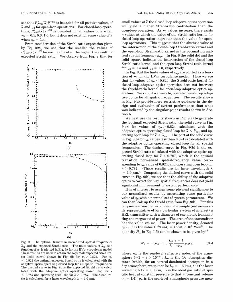
Fig. 9. The optimal transition normalized spatial frequencieskop and the expected Strehl ratio. The finite values of kop as afunction of h0 is plotted in Fig. 9a for the HV5/7 turbulence model.These results are used to obtain the (optimal) expected Strehl ra-tio (solid curve) shown in Fig. 9b for h0 . 0.824. For h0< 0.824 the optimal expected Strehl ratio is calculated with theadaptive optics operating closed loop for all spatial frequencies.The dashed curve in Fig. 9b is the expected Strehl ratio calcu-lated with the adaptive optics operating closed loop for k, 0.787 and operating open loop for k . 0.787. The Strehl ra-tio is calculated for a laser wavelength l 5 1.0 mm.

small values of k the closed-loop adaptive-optics operationwill yield a higher Strehl-ratio contribution than theopen-loop operation. As h0 values increase, there existsk values at which the value of the Strehl-ratio kernel forclosed-loop operation is greater than the value for open-loop operations. This suggests that the abscissa value ofthe intersection of the closed-loop Strehl-ratio kernel andthe open-loop Strehl-ratio kernel is the optimal normal-ized spatial frequency kop . In Fig. 8 the solid dot and thesolid square indicate the intersection of the closed-loopStrehl-ratio kernel and the open-loop Strehl-ratio kernelfor h0 5 1.4 and h0 5 1.0, respectively.

In Fig. 9(a) the finite values of kop are plotted as a func-tion of h0 for the HV5/7 turbulence model. Here we seethat for values of h0 , 0.824, the Strehl-ratio kernel forclosed-loop adaptive optics operation does not intersectthe Strehl-ratio kernel for open-loop adaptive optics op-eration. We can, if we wish to, operate closed-loop adap-tive optics for all spatial frequencies. The results shownin Fig. 9(a) provide more restrictive guidance in the de-sign and evaluation of system performance than whatwas indicated by the singular-point results shown in Sec-tion 5.

We next use the results shown in Fig. 9(a) to generatethe (optimal) expected Strehl ratio [the solid curve in Fig.9(b)] for values of h0 . 0.824 calculated with theadaptive-optics operating closed loop for k < kop , and op-erating open loop for k . kop . The part of the solid curvein Fig. 9(b) for h0 values less than 0.824 is calculated withthe adaptive optics operating closed loop for all spatialfrequencies. The dashed curve in Fig. 9(b) is the ex-pected Strehl ratio calculated with the adaptive optics op-erating closed loop for k , 0.787, which is the optimaltransition normalized spatial-frequency value corre-sponding to h0 value of 0.824, and operating open loop fork . 0.787. (These results are for laser wavelength l5 1.0 mm.) Comparing the dashed curve with the solid

curve in Fig. 9(b), we see that the ability of the adaptiveoptics to correct for high spatial frequencies does not yieldsignificant improvement of system performance.

It is of interest to assign some physical significance toour normalized results by associating some particularvalue of h0 with a nominal set of system parameters. Wecan then look up the Strehl ratio from Fig. 9(b). For thispurpose we consider as a nominal example (not necessar-ily representative of any particular system of interest) aHEL transmitter with a diameter of one meter, transmit-ting one megawatt of power. The area of the transmitterhas the value p/4 m2. The laser power density, denotedby I0, has the value 106/(p/4) 5 1.273 3 106 W/m2. Thequantity Nl in Eq. (15) can be shown to be given by15

Nl 5 2~n0 2 1 !L0

l

g 2 1gp0

m0I0, (85)

where n0 is the sea-level refractive index of the atmo-sphere ('1 1 3 3 1024), L0 is the 1/e absorption dis-tance (which, for an aerosol-dominated absorption in adry atmosphere, we take to be L0 5 1.5 km), l is the laserwavelength (l 5 1.0 mm), g is the ideal gas ratio of spe-cific heat at constant pressure to that at constant volume(g 5 1.4), p0 is the sea-level atmospheric pressure mea-


sured in newtons per square meter ( p0 ' 105 N m22),and m0 is the atmospheric absorptivity at sea level, whichfor dry atmosphere aerosol-dominated absorption we taketo be m0 ' 8.667 3 1026 m21. When we substitute thesevalues into Eq. (85), we obtain Nl 5 14.19 waves s21.The Fresnel scale length, L0 5 (lL0)1/2, has a value ofL0 5 @(1.0 3 1026) 3 (1.5 3 103)#1/2 5 0.0387 meter.We shall use an estimated value16 for the velocity struc-ture constant of CV

2 5 4.0 3 1022 m2/3/s, so the normal-ized time t0, as defined in Eq. (14), has a value t05 [email protected] 3 1022(1.5 3 103)1/3#21 5 0.0845 s. TheWISP number h0, as defined in Eq. (16), has a value ofh0 5 14.19 3 0.0845 5 1.20. From Fig. 9 we can thenconclude that an ideal phase-only adaptive optics one-meter diameter HEL transmitter, transmitting one mega-watt power, can have a Strehl ratio of 0.84 for the HV5/7turbulence model, provided that the adaptive optics doesnot correct for spatial frequencies higher than k5 0.545. [Using the value of L0 5 0.0387 m, we can de-termine that this requirement of the adaptive-opticsspatial-frequency transition corresponds to an actuatorspacing of 0.0355 m, which is significantly smaller thanwhat the r0 value ('0.115 m for the HV5/7 turbulencemodel) would nominally cause us to use.]

These results show that the adaptive optics thermal-blooming interaction—as ameliorated by wind shear—need not have a severe effect on high-energy laser atmo-spheric propagation insofar as deliverable performance inthe far field is concerned. Other effects such as finiteservo bandwidth, realistic hardware effects [e.g., finiteadaptive-optics element (detector) size], slewing beams,and finite wind-clearing time for small aperture applica-tions may further relax the phase-compensation stabilityrequirements, so system performance will undoubtedlyvary somewhat from the result indicated by Fig. 9. Butfor many (perhaps most) cases of interest, avoiding PCIwill not be a problem.

7. SUMMARYWe have presented both the time-dependent and thesteady-state analyses of the effects of wind shear onphase-compensation instability for high-energy laserbeam propagation in a turbulent atmosphere. By prop-erly modeling the fine-scale physics of the random wind inthe heating-transport equation, our time-dependent solu-tions conclusively show the true manifestation of PCI andindicate the existence of a large parameter space in whichPCI does not occur. Our steady-state analysis permits usto evaluate the allowable laser power density as a func-tion of spatial frequency for PCI-free adaptive-optics op-erations. By determining the optimal range of spatialfrequencies for closed-loop adaptive-optics operation, wecan evaluate the achievable expected Strehl ratio for anominal case of interest.

ACKNOWLEDGMENTSThe work was done while both authors were at the Opti-cal Sciences Company. This work was performed in sup-port of the PCAP activity conducted by the U.S. Air Forceat the Phillips Laboratory, Kirtland Air Force Base. Wewish to acknowledge the interactions with members of thePCAP activity group and to some extent the work groupassociated with the part of the GBFEL/TIE program thatwas concerned with the study of adaptive optics and high-energy laser beam propagation through the atmosphere.Our interactions helped us greatly in forcing the formula-tion and the development of the results presented in thiswork.

REFERENCES1. T. J. Karr, ‘‘Thermal blooming compensation instabilities,’’

J. Opt. Soc. Am. A 6, 1038–1048 (1989).2. S. Enguehard and B. Hatfield, ‘‘Perturbative approach to

the small-scale physics of the interaction of thermal bloom-ing and turbulence,’’ J. Opt. Soc. Am. A 8, 637–646 (1991).

3. J. F. Schonfeld, ‘‘Linearized theory of thermal-bloomingphase compensation instability with realistic adaptive-optics geometry,’’ J. Opt. Soc. Am. B 9, 1803–1812 (1992).

4. V. Lukin and B. Fortes, ‘‘The influence of wavefront dislo-cations on phase conjugation instability at thermal bloom-ing compensation,’’ Pure Appl. Opt. 6, 103–116 (1997).

5. D. G. Fouche, C. Higgs, and C. F. Pearson, ‘‘Scaled atmo-spheric blooming experiments (SABLE),’’ The Lincoln Labo-ratory J. 5, 273–292 (1992).

6. D. L. Fried, ‘‘Blurring effects in thermal blooming,’’ tOSCTech. Report TR-902 (Optical Sciences Company, Anaheim,Calif., August 1988).

7. D. L. Fried and R. K. Szeto, ‘‘Turbulence and thermalblooming interaction (TTBI): static,’’ tOSC Tech. ReportTR-921 (Optical Sciences Company, Anaheim, Calif., Sep-tember 1988).

8. V. I. Tatarskii, The Effects of the Turbulent Atmosphere onWave Propagation (National Technical Information Service,Springfield, Va., 1971).

9. R. K. Szeto and D. L. Fried, ‘‘Mini-shear effects and PCI,’’tOSC Tech. Report TR-1076 (Optical Sciences Company,Anaheim, Calif., July 1990).

10. H. B. Keller, ‘‘A new difference scheme for parabolic prob-lems,’’ in Numerical Solutions of Partial Differential Equa-tions II, B. Hubbard, ed. (Academic, New York, 1971).

11. Work is currently in preparation by R. Szeto on numericalmodeling of small-scale physics in atmospheric-turbulencepropagation.

12. R. K. Szeto and D. L. Fried, ‘‘Steady state TTBI singularpoints and PCI thresholds,’’ tOSC Tech. Report TR-1083(Optical Sciences Company, Anaheim, Calif., August 1990).

13. D. E. Novoseller, TRW, Redondo Beach, Calif. 90278 (per-sonal communication; letter to P. Berger, copy to tOSC,dated July 1, 1991).

14. D. L. Fried, ‘‘Optical resolution through a randomly inho-mogeneous medium for very long and very short expo-sures,’’ J. Opt. Soc. Am. 56, 1372–1379 (1966).

15. J. L. Walsh and P. B. Ulrich, ‘‘Thermal blooming in the at-mosphere,’’ in Laser Beam Propagation in the Atmosphere,J. W. Strohbehn, ed. (Springer-Verlag, New York, 1978).

16. D. L. Fried, ‘‘Analysis of turbulence velocity spread data,’’tOSC Tech. Report TR-923 (Optical Sciences Company,Anaheim, Calif., September 1988).

Wind-shear induced stabilization of PCI

Documents

Transcript of Wind-shear induced stabilization of PCI