UNIVERSIDAD COMPLUTENSE DE MADRID

FACULTAD DE CIENCIAS FÍSICAS Departamento de Física de la Tierra, Astronomía y Astrofísica II

STATISTICAL DOWNSCALING OF SURFACE WIND FIELD AND WIND ENERGY OVER A

COMPLEX TERRAIN AREA.

MEMORIA PARA OPTAR AL GRADO DE DOCTOR

PRESENTADA POR

Elena García Bustamante

Bajo la dirección de los doctores

J. Fidel González Rouco Jorge Navarro Montesinos

Madrid, 2011

ISBN: 978-84-694-2808-5 © Elena García Bustamante, 2010

� �

Statistical downscaling of surface wind fieldand wind energy over a complex terrain area

Estimacion estadıstica del viento en superficie yde la energıa eolica en una region de terreno

complejo

Memoria que presenta

Elena Garcıa Bustamante

para optar al grado de

Doctor en Ciencias Fısicas

Directores:

Dr. J. Fidel Gonzalez RoucoDr. Jorge Navarro Montesinos

Departamento de Fısica de la Tierra, Astronomıa y Astrofısica IIFacultad de Ciencias FısicasUniversidad Complutense de Madrid

II

Convienen los fısicos en que el viento es un movimiento sensibledel aire; y no es dudable, pues el simple movimiento que puededarle un abanico hace un viento bien perceptible. Puede estemovimiento venir de qualquiera parte, ası pueden ser tantas lasdiferencias de los vientos, si se examinan fısicamente, quanto sonlos puntos sensibles del Horizonte. [...] Sospecho que ası comola luz excita al fuego, conmueve tambien al aire, y que muchosefectos admirables que tenemos delante de los ojos, y ignoramossus causas, nacen de las operaciones recıprocas de los elementos.Con esto se explica la formacion de los vientos continuos, yperiodicos que se observan en varios lugares. [...] Pueden losvapores excitar el viento empujando el aire y obligandole aceder a su fuerza, y esta es la causa mas comun de los vientos.Finalmente el fuego puede causar los vientos, dilatando el aire,y aflojando sus muelles. [...] El Sol excita al fuego, levanta losvapores, y hace vibrar la luz; ası pone en accion todas las causasproximas de los vientos, y sus mudanzas. [...] Hemos explicado lascausa generales de los vientos, pero haciendo variar de muchosmodos sus operaciones, la situacion de los montes, valles, maresy otras muchas cosas propias del clima, es preciso explicarlasacomodandonos a estas particularidades. [...] Si estas causas secombinan de muchas maneras, pueden hacer mucha variedad enlos vientos, que solamente podran atinarse con la observacioncuidadosa de los lugares y los tiempos.

Dr. A. Piquer. Fısica Moderna, Racional y Experimental, 1745.

Contents

List of acronyms . . . . . . . . . . . . . . . . . . . . . . . . . . . . . . . . . . . . . . . . . . . . . . . . . XI

Summary . . . . . . . . . . . . . . . . . . . . . . . . . . . . . . . . . . . . . . . . . . . . . . . . . . . . . . . . XV

Resumen . . . . . . . . . . . . . . . . . . . . . . . . . . . . . . . . . . . . . . . . . . . . . . . . . . . . . . . . XIX

1 Introduction . . . . . . . . . . . . . . . . . . . . . . . . . . . . . . . . . . . . . . . . . . . . . . . . . 11.1 Nature of the cross-scales problem: assessing regional climate

variability . . . . . . . . . . . . . . . . . . . . . . . . . . . . . . . . . . . . . . . . . . . . . . . . 21.2 Uncertainty in downscaling estimations . . . . . . . . . . . . . . . . . . . . . . . 61.3 Impact oriented studies . . . . . . . . . . . . . . . . . . . . . . . . . . . . . . . . . . . . 81.4 Objectives and structure . . . . . . . . . . . . . . . . . . . . . . . . . . . . . . . . . . . 10

2 Observational datasets . . . . . . . . . . . . . . . . . . . . . . . . . . . . . . . . . . . . . . . 152.1 Climatology of the CFN . . . . . . . . . . . . . . . . . . . . . . . . . . . . . . . . . . . . 152.2 Observed wind speed and wind power at the wind farm locations 182.3 Observed wind field in the CFN . . . . . . . . . . . . . . . . . . . . . . . . . . . . . 232.4 Large scale fields . . . . . . . . . . . . . . . . . . . . . . . . . . . . . . . . . . . . . . . . . . 28

Part I Relationship between wind speedand wind power

3 The influence of the Weibull assumption in monthly windenergy estimation . . . . . . . . . . . . . . . . . . . . . . . . . . . . . . . . . . . . . . . . . . . . 333.1 Rationale: the need of assessing wind speed distributions . . . . . . . 34

IV Contents

3.2 Preliminary aspects of the wind-wind power relation: analysis ofobservations . . . . . . . . . . . . . . . . . . . . . . . . . . . . . . . . . . . . . . . . . . . . . . 36

3.3 Methodology . . . . . . . . . . . . . . . . . . . . . . . . . . . . . . . . . . . . . . . . . . . . . . 423.3.1 Fitting to the Weibull probability distribution . . . . . . . . . . 45

3.4 Analysis of results . . . . . . . . . . . . . . . . . . . . . . . . . . . . . . . . . . . . . . . . . 473.4.1 Errors in wE estimation . . . . . . . . . . . . . . . . . . . . . . . . . . . . . . 473.4.2 Goodness of fit . . . . . . . . . . . . . . . . . . . . . . . . . . . . . . . . . . . . . . 52

3.5 Conclusions . . . . . . . . . . . . . . . . . . . . . . . . . . . . . . . . . . . . . . . . . . . . . . . 58

4 A comparison of methodologies for monthly wind energyestimation . . . . . . . . . . . . . . . . . . . . . . . . . . . . . . . . . . . . . . . . . . . . . . . . . . . 614.1 The rationale . . . . . . . . . . . . . . . . . . . . . . . . . . . . . . . . . . . . . . . . . . . . . 624.2 Analysis of methodologies . . . . . . . . . . . . . . . . . . . . . . . . . . . . . . . . . . 63

4.2.1 Estimation based on hourly resolution data . . . . . . . . . . . . . 644.2.2 Interpolation using the theoretical power curve . . . . . . . . . . 684.2.3 Linear regression . . . . . . . . . . . . . . . . . . . . . . . . . . . . . . . . . . . . 70

4.3 Results and discussion . . . . . . . . . . . . . . . . . . . . . . . . . . . . . . . . . . . . . 734.3.1 Estimations based on hourly data . . . . . . . . . . . . . . . . . . . . . 734.3.2 Estimations with monthly data and comparison with the

hourly case . . . . . . . . . . . . . . . . . . . . . . . . . . . . . . . . . . . . . . . . . 784.4 Conclusions . . . . . . . . . . . . . . . . . . . . . . . . . . . . . . . . . . . . . . . . . . . . . . . 81

Part II Wind and wind power dependence onlarge scale atmospheric circulation

5 North Atlantic atmospheric circulation and surface wind inthe Northeast of the Iberian Peninsula . . . . . . . . . . . . . . . . . . . . . . 855.1 The regional climate problem: the role of the downscaling

techniques . . . . . . . . . . . . . . . . . . . . . . . . . . . . . . . . . . . . . . . . . . . . . . . . 865.2 Downscaling methodology . . . . . . . . . . . . . . . . . . . . . . . . . . . . . . . . . . 895.3 Wind estimations in the CFN: the reference case . . . . . . . . . . . . . . 91

5.3.1 Canonical patterns and series . . . . . . . . . . . . . . . . . . . . . . . . . 925.3.2 Validation of wind estimates . . . . . . . . . . . . . . . . . . . . . . . . . . 97

5.4 Uncertainty analysis . . . . . . . . . . . . . . . . . . . . . . . . . . . . . . . . . . . . . . . 1005.4.1 Methodological uncertainty . . . . . . . . . . . . . . . . . . . . . . . . . . . 1005.4.2 Single and multi-data experiments . . . . . . . . . . . . . . . . . . . . . 106

5.5 Wind field long term variability: a wind climatology reconstruction1095.6 Conclusions . . . . . . . . . . . . . . . . . . . . . . . . . . . . . . . . . . . . . . . . . . . . . . . 115

Contents V

6 Relationship between wind power production and NorthAtlantic atmospheric circulation . . . . . . . . . . . . . . . . . . . . . . . . . . . . . 1196.1 The wind power production as an impact variable . . . . . . . . . . . . . 1206.2 Statistical downscaling of wind power production . . . . . . . . . . . . . . 1226.3 Alternative methods for the estimation of wind power production 1266.4 Applications: estimating wind power in the absence of observations1316.5 Conclusions . . . . . . . . . . . . . . . . . . . . . . . . . . . . . . . . . . . . . . . . . . . . . . . 135

7 Bayesian uncertainty in downscaled wind field estimations . . . 1397.1 Motivation . . . . . . . . . . . . . . . . . . . . . . . . . . . . . . . . . . . . . . . . . . . . . . . 1407.2 Methodology: the Bayesian framework . . . . . . . . . . . . . . . . . . . . . . . 142

7.2.1 Prior probabilities . . . . . . . . . . . . . . . . . . . . . . . . . . . . . . . . . . . 1437.2.2 Likelihood function . . . . . . . . . . . . . . . . . . . . . . . . . . . . . . . . . . 1447.2.3 Marginal posterior distribution . . . . . . . . . . . . . . . . . . . . . . . . 1457.2.4 Autocorrelation . . . . . . . . . . . . . . . . . . . . . . . . . . . . . . . . . . . . . 146

7.3 Results and discussion . . . . . . . . . . . . . . . . . . . . . . . . . . . . . . . . . . . . . 1477.3.1 Some insight into the parameter rejection areas . . . . . . . . . 1477.3.2 Posterior distributions . . . . . . . . . . . . . . . . . . . . . . . . . . . . . . . 1527.3.3 Sensitivity to prior knowledge . . . . . . . . . . . . . . . . . . . . . . . . . 158

7.4 Conclusions . . . . . . . . . . . . . . . . . . . . . . . . . . . . . . . . . . . . . . . . . . . . . . . 161

8 Conclusions and discussion . . . . . . . . . . . . . . . . . . . . . . . . . . . . . . . . . . 1658.1 Conclusions . . . . . . . . . . . . . . . . . . . . . . . . . . . . . . . . . . . . . . . . . . . . . . . 1668.2 Quo Vadis? . . . . . . . . . . . . . . . . . . . . . . . . . . . . . . . . . . . . . . . . . . . . . . . 1698.3 A discourse on related topics . . . . . . . . . . . . . . . . . . . . . . . . . . . . . . . . 173

8.3.1 Need of observations . . . . . . . . . . . . . . . . . . . . . . . . . . . . . . . . . 1738.3.2 Energy: sources and demand . . . . . . . . . . . . . . . . . . . . . . . . . . 1748.3.3 Science and society . . . . . . . . . . . . . . . . . . . . . . . . . . . . . . . . . . 1758.3.4 A case study? . . . . . . . . . . . . . . . . . . . . . . . . . . . . . . . . . . . . . . . 178

Appendix A . . . . . . . . . . . . . . . . . . . . . . . . . . . . . . . . . . . . . . . . . . . . . . . . . . . . . 181The Fisher distribution and the estimation of degrees of freedom . . . . . 181Combinations of the statistical downscaling model parameters . . . . . . . 186

References . . . . . . . . . . . . . . . . . . . . . . . . . . . . . . . . . . . . . . . . . . . . . . . . . . . . . . . 189

Glossary . . . . . . . . . . . . . . . . . . . . . . . . . . . . . . . . . . . . . . . . . . . . . . . . . . . . . . . . . 211

Agradecimientos

Sentirse agradecido, dar las gracias, no es un mero formalismo. Agradecer sig-nifica sentirse afortunado de haber tenido la oportunidad de recibir algo bueno.Tambien significa reconocerse limitado y, sin embargo, disfrutar de saber quedonde uno no llega, llegan los demas. Es ası como, de la mano de los que algunao muchas veces nos la tendieron, se llega a donde uno piensa que merecıa la penallegar. El camino que he recorrido a lo largo de estos anos de tesis ha sido unaexperiencia valiosa y esta es una ocasion bonita para expresarlo. Hay muchaspersonas a las que me gustara decir gracias por haber andado conmigo alguntrecho de ese camino o buena parte de el. De todas ellas no quisiera dejar demencionar a las siguientes:

A Elena, mi madre, quiero agradecerle su bondad infinita y fruto de ella, sucomprension sin lımites. Ademas, su paciencia, su generosidad y desprendimiento,su discrecion, su sencillez, su fuerza... podrıa seguir... me impresionan profunda-mente y son un referente para mi. Gracias por compartir conmigo todos esosviajes.

A Pedro, mi padre, quisiera darle gracias por su apoyo incondicional. Igualespero distintos, hemos encontrado un espacio en el que aprender el uno del otro.Su vastısima cultura, sus ansias de saber y su curiosidad vital inclinan la balanzade su lado, sin duda quien mas ha aprendido del otro he sido yo. A el y a superenne mensaje “persevera en aquello que tu creas que es bueno conseguir.. ydisfrutalo..”. Gracias por hacerme saber que siempre estabas ahı detras, en laretaguardia, por si acaso...

A Bea, mi hermana, que me quiere tanto y me lo dice siempre, a su frescuray su naturalidad que no las he visto antes, a sus consejos de hermana mayor,

suya es la primera mano que recuerdo, a sus risas, a su instinto protector y a lasensacion de seguridad que transmite, porque al lado de Bea todo parece ir bien.

A Fidel, mi maestro y mi amigo. Para agradecerle todo lo que me haensenado tendrıa que escribir otro libro con tantas paginas como este. Su ge-nerosidad hacia todos, sin distinciones, su humildad sin precedentes y su pasionpor aprender debieran ser quiza objeto de algun estudio cientıfico. Fidel es elartıfice de este trabajo, el que hacıa las cosas posibles cuando parecıa que no loeran. Con Fidel he aprendido infinitas cosas de valor incalculable, pero quieroresaltar el haber aprendido de el lo provechoso de un uso delicado del lenguage:para atreverse siempre a decir lo que uno piensa, para dar razones y argumen-tos, para dar forma a las ideas, para preguntar cuando surgen las dudas, usarel lenguaje para dar opciones, para acoger y respetar otras opiniones... no hablosolo de ciencia. He disfrutado mucho de su amistad, a traves de la cual he descu-bierto la increıble cantidad de dimensiones distintas que puede llegar a tener unapersona, ası es como conocı tambien al dios de la semisatisfaccion y los intentosde conjurarlo... Gracias Fidel por no ponerle nunca precio a tu tiempo.

A Jorge, que me ha apoyado sin condiciones desde aquel primer dıa. Elme ha transmitido siempre su confianza en mi, no solo con palabras, tambiencuidando cada detalle hasta el final, haciendo posible la continuidad del trabajo,asegurando la estabilidad mas de mil veces. Sin Jorge nada de esto habrıa sidoposible. Ademas el es la alegrıa en persona, sabe gestionar cada situacion desdela creencia de que todo tiene solucion, que las cosas pueden salir bien. ¡Que suertehaberle encontrado! Gracias Jorge.

A Marisa, a la que admiro profundamente desde que la conocı. Marisa esuna mujer irrepetible, una luchadora incansable, es justa como pocos, de esaspersonas que inspiran, cuando uno ve a Marisa hacer ciencia quiere imitarla. Ellapiensa en todos y se preocupa por todos y a mi en concreto me ha ayudado enincontables ocasiones. No se como habrıa sido esto sin Marisa.

A Pedro, mi companero, al que aun no me he acostumbrado a no tener cerca.Comenzamos esta andanza como companeros de fatigas y se convirtio tambienen un maestro para mi. Todo lo que fue aprendiendo me lo transmitio comohermano mayor. Pedro es un cientıfico de lo clasicos, para el llegar a entender lascosas mas sencillas supone un triunfo y una fiesta, siempre interprete eso comoun rasgo de su inteligencia. Todavıa puedo verle observando fijamente la pantallade su ordenador. Gracias por ensenarme a no tener prisa.

A Angela, el experimento: amiga desde hace anos y ahora companera enel trabajo. Nada de lo que diga aquı es suficiente para agradecerle su paciencia.Angela me aporta cosas siempre, todos los dıas, es creativa, es crıtica, tieneideas, organiza.. Y sobre todo, me cuida, cuida de mi constantemente. Angela

Agradecimientos IX

es mi familia. ¿Como puedo agradecerte todo eso amiga? Desde luego no pareceposible con palabras, pero aun ası quisiera decirlo, gracias por estar a mi lado.

A Juanpe, a su don para intercalar ciencia y alegrıa, que me enseno apacientemente a hacer integraciones con MM5, a mi y a tantos, que siempre estaal otro lado del telefono, no importa que hora sea, con una opinion. Juanpe haparticipado con constancia en todos y cada uno de los trabajos, en las tesis, enGlobal, en las publicaciones.. no recuerdo un solo correo no contestado, siemprecrıtico, no es facil sesgar a Juanpe. ¿Cuantas cervezas habremos compartido?¿Cuantas ideas salieron de ellas? Todo un lujo y un placer ser de tu equipo.

A mis amigos del laboratorio: a Pablete y su sentido del humor refinado,siempre un juego de palabras a la orden del dıa ; a Laura, que cuando entra porla puerta es como si amaneciera; a Etor, autentico y original, no hay nadie comoEtor, gracias por tus quijotes “ilustrados”; a Ruben, siempre dipuesto a unasrisas, cuanta sensatez se le adivina aun sin necesidad de hablar ¡lo que da SanMartın de Valdeiglesias!; a Roland, que solıa saberlo todo sobre linux y siemprequerıa saber mas y que nos contaba con ilusion sus viajes; a German, tan sincero,que siempre me regana cuando le doy las gracias, ¡gracias German!; a Jose, tandiscreto y tan carinoso; a Volker, sus libros y sus discos, gracias por compartirlosconmigo. A todos vosotros que habeis hecho posible un ambiente de trabajo unicoy que dıa tras dıa y, muchas veces, noche tras noche, os he visto sacar lo mejorcitode vosotros mismos, de todo corazon, gracias.

A Elena, a su efervescencia y a su espıritu infatigable. Elena no dudo enacogerme en su casa y en tratarme desde el primer dıa como a una amiga, como auna hermana y como a una hija, triple dimension de carino, casi inverosımil. Nosolo me ha cuidado en lo personal, tambien ha cuidado de nuestro trabajo hastala ultima palabra, participando en las discusiones, aportando ideas, leyendonos,corrigiendonos, planteando estrategias. Gracias Elena por todo esto y por las inol-vidables noches de primavera suizas de vino y jazz. Y gracias a Juerg, her belovedhusband, una persona calida, acogedora al mas puro estilo Xoplaki-Luterbacher,delicado en el trato con todos, sobre todo con sus estudiantes, alguien que seinteresa por tus cosas al minuto de conocerte, de conversacion facil y agradable...vaya dos...

A Nacho, mi amigo, mi companero de toda la vida, hemos visto pasar pornuestro lado toda clase de tormentas y tempestades y no hemos tenido miedode explorar a donde nos llevaban todos esos vientos, los dos hemos crecido de lamano. Nacho lleva anos preocupandose con ternura de las horas que duermo yde si bebo o no agua. Pero lo mejor de todo es cuanto me hace reir. Gracias portu musica, gracias por la bicicleta y gracias por ponerme en la catapulta, porconducirme a descubrir que uno puede ser y hacer cosas, muchas cosas...

A mis amigos, a la suerte de haberlos encontrado: Raquel, la eficiencia, queme ensena a buscar una actitud coherente y a cuestionar cosas viejas; a MiguelAngel, el cunao, a su vitalidad y su cultura de dimensiones desconocidas por elser humano, a las cuerdas de su guitarra; a Laura, la pequena, a su intuicionque siempre acierta, a su ser sin prisas (¡que bien haber llegado juntas a esto!); aAngela, a quien ya he nombrado y que merece ocupar tambien este puesto, a lasrisas juntas, esas noches de risas casi por los suelos, los viajes; a Estrella, la masantigua, con quien descubrı esta ciudad, que me dejaba sentarme a su ordenadorcuando querıa ordenar las ideas y me desvelaba las ventajas de pensar las cosasdos veces, en silencio o no, siempre a mi lado; a Marine y su espıritu positivo,¡una valiente! Quisiera estar cerca de ellos siempre.

A M. Isabel, que me enseno lo que significa la honradez en el trabajoentre tantas otras cosas y que me hizo disfrutar de las matematicas, misteriosahabilidad la que ella tiene para mostrar el lado luminoso de las cosas, que meacerco a la fısica sin darse cuenta.

A Eugenia, Lucıa y Antonio, por su disponibilidad todos los dıas, por sudescomunal eficacia. A Paul, Nico, Miguel, Fernando y Jorge, por vuestra ayuday los buenos ratos. A Paco, Alfonso, Ana, Carolina, Carmen, Pedro, David, Ma-riano, el Pive, Isabel y, en general, a todos los chicos de la facultad, me habeishecho sentir como en casa.

List of acronyms

APC Average Power Curveβ Brier skill scorec Weibull scale parameterCCA Canonical Correlation AnalysisCCApow CCA with the wind power as predictandCCApow−mod wind module CCA and wind-wind power

linear transferCCApow−uv wind components CCA and wind-wind power

linear transferCCApow−reg wind module CCA and regional wind-wind power

linear transferCFN Comunidad Foral de NavarraCIEMAT Centro de Investigaciones Energeticas,

Medioambientales y TecnologicasCp Power coefficientD data or observationsEA East Atlantic patternEA/WR East Atlantic/Western Russian patternECMWF European Center for Medium-range Weather ForecastENSO EL Nino Southern OscillationEOF Empirical Orthogonal FunctionEPC Effective Power Curveφ850 850 hPa geopotential heightφ850 500 hPa geopotential heightf(wi) wind speed frequencies for the i class interval

GCM General Circulation ModelF Fisher distributionHadSLP2 Hadley Centre SLP observations version 2Hi a prior hypothesisIP Iberian Peninsulak Weibull shape parameterκ Number of EOFs/CCAs retained in the statistical

downscaling model (Ch. 7)µ Large scale domain size in the statistical downscaling model (Ch. 7)MOS Model Output StatisticNAO North Atlantic OscillationNCAR National Center for Atmospheric Researchneff Effective sampled size after corrections based on serial

autocorrelationP actual power produced by a wind turbinePa available power carried by the windPDF Probability Density Functionp(Hi) prior probability of the hypothesisp(D|Hi) probability of obtaining data D, supposed Hi is true (likelihood)p(Hi|D) marginal posterior probability of Hi

PLinear monthly linearly fitted power outputPInterp monthly interpolated power outputpout(wi) transfer function for the power vs. wind speed relation for a given wi

Pw wind power generated by an ideal wind turbineP(µ) prior probability distribution of the large scale domain sizeP(σ) prior probability distribution of the predictor field(s) (Ch. 7)P(κ) prior probability distribution of the number of EOFs/CCAs

patterns retainedP(θ) prior probability distribution of the number of crossvalidation

subset sizep(µ, σ, ρ, θ|D) joint marginal posterior distribution of the parameters

µ, σ, ρ and θPFC Polynomial Fit Curver(µ, σ, ρ, θ) residual (obs. minus est.) for the combination of parameters

µ, σ, ρ and θ||r||2 sum of square residuals for all time steps

List of acronyms XIII

||rmin||2 minimum sum of square residualsρ correlation skill scoreRCM Regional Circulation ModelR2 statistic for the evaluation of the parameters rejection areasRera40 wind field reconstructions based on ERA-40 SLPRpower−era40 wind energy reconstructions based on ERA-40 SLPRhad wind field reconstructions based on HadSLP2

observationsRpower−had2 Wind energy reconstructions based on HadSLP2

observationsRLuterb wind field reconstructions based on Luterb. et al. (2002)

SLP recon.Rncar wind field reconstructions based on NCAR SLP

observationsRpower−ncar wind energy reconstructions based on NCAR SLP

observationsσ predictor field(s) in the statistical downscaling (Ch. 7)

modelSCAND Scandinavian patternSLP Sea level pressureSwm

monthly mean wind speed standard deviationSwEm

monthly mean wind energy standard deviationTPC Theoretical Power Curveθ crossvalidation sample size in the statistical (Ch. 7)

downscaling modelU10 zonal component of the wind at 10 mUCM Universidad Complutense de MadridV10 meridional component of the wind at 10 mw wind speedwi wind speed representative for the i class intervalw monthly mean wind speedwE wind energywELinear total monthly wind energy from the monthly linear fitwEInterp total monthly wind energy from the monthly interpolation

wEH−EPCwtotal monthly wind energy from hourly wind speedusing the EPC and the Weibull expected frequencies

wEH−APC total monthly wind energy from hourly wind speedusing the APC

wEH−APCwas the previous but with Weibull expected frequencies

wEH−PFC total monthly wind energy estimated from hourly windspeed using the PFC

wEH−ref total monthly wind energy estimated from hourly windspeed using the EPCs

wEm monthly mean wind energyξi wind energy estimation error using the i method (Ch. 4)Z500−850 thickness between 500 and 850 hPa geopotential heights

Summary

The assessment of the wind field variability at the regional/local scale involvesmany challenging scientific questions concerning the multiple interactions be-tween large and local scales that give rise to the large spatio-temporal variabilityof the wind field, especially over complex terrain regions. Additionally, the evalu-ation of the surface wind circulations entails interesting applications for society:insurance companies, air-quality or health oriented studies as well as wind energyproduction, that require accurate estimates from the short term predictions tothe long term sustainability assessments. These are some examples that demandknowledge about the wind field circulation at the regional/local scales.

This work pursues two main objectives. One of them is the evaluation of therelation between wind and wind power. The second objective is the analysis ofthe coupled variability between the regional surface wind field and wind powerproduction in the northeast of the Iberian Peninsula and the large scale circula-tion over the North Atlantic and Mediterranean areas. The results obtained inthe first part of the work evidence a linear relationship between wind and windpower that supports the exploration of dependencies of both variables with thelarge scale circulation in the second part of the text.

Surface wind field observations for the period 1992-2005 are recorded at 29meteorological stations homogeneously distributed around the target region (Co-munidad Foral de Navarra; CFN). In addition, wind and wind power records areavailable at five wind farms within the region for the period 1999-2003. All ob-served series were subject to quality assurance processes to guarantee the qualityof the observations that are the inputs in the different analyses.

The relation between wind and wind power is explored on the basis of theanalysis of classical methodologies to estimate wind energy. The different contri-butions to the error in wind energy estimations are evaluated. Two main sources

of error are explored: the representation of the observed wind frequencies bya theoretical distribution and the contribution due to the assumed wind-windpower transfer function. It is shown that the typical Weibull assumption appliedto estimate wind frequencies does not hold at every site or time step, howeverthe resulting errors are not large due to a partial cancellation of residuals withdifferent sign. The larger contribution to the errors arises from the use of trans-fer functions to translate wind into wind power values. Different alternativeswere tested and a simpler linear relation between monthly wind-wind power val-ues proves a good performance in estimating monthly wind energy compared toother more elaborated approaches. It also represents the basis to explore in thesecond part of the work the performance of a statistical downscaling techniqueapplied to estimate wind power from changes in the large scale.

The connection between the variability of the wind field at the CFN and thelarge scale atmospheric circulation is investigated through the application of astatistical downscaling approach (Canonical Correlation Analysis). To a large ex-tent, the variability of the wind at monthly timescales is found to be governedby the large scale circulation modulated by the particular orographic features ofthe area. The sensitivity of the downscaling methodology to the selection of themodel parameter values is explored, in a second step, by performing a system-atic sampling of the parameter space. This provides a metric for the uncertaintyassociated with the various possible model configurations. This uncertainty isconsiderably dependent on the spatial variability of the wind. While the sam-pling of the parameter space in the model set up moderately impacts estimationsduring the calibration period, the regional wind variability is very sensitive tothe parameter selection at longer timescales. This fact illustrates that downscal-ing exercises based on a single configuration of parameters should be interpretedwith extreme caution. The downscaling model is used to extend the estimationsseveral centuries to the past using long datasets of sea level pressure, therebyillustrating the large temporal variability of the regional wind field from interannual to multi centennial timescales.

Based on the linear relation between the wind and the wind power found inthe first part of the text, the downscaling approach is extended to the case of thewind power as a non-meteorological variable. This can be ascribed to the contextof impact oriented studies. It is shown that the variability of the wind power inthe region is connected to variations of the large scale circulation over the NorthAtlantic areas. Alternative procedures that estimate first the wind over the regionand then translate it into wind power estimates using the linearity between bothvariables, prove useful in practical situations where no wind power records areavailable. The uncertainty associated to the wind power estimations is identicallyexplored herein as in the case of the wind field.

Summary XVII

Finally, a probabilistic approach to evaluate the impact of each parameter ofthe model configuration on the wind field estimates is analysed. The treatment ofuncertainties is based on the Bayesian theory and it consists in assigning weightsto each parameter value depending on its ability to produce wind estimationsin good agreement with observations. The ability of the method to identify theoptimal model configurations or to detect parameters with a robust response tochanges in the rest of the parameters is discussed.

This work provides therefore a description of a sequence of experiments posedfrom different, albeit connected, approaches targeting a better understanding ofthe variability of the wind and wind power over a region of complex terrain. Indoing so, this text offers the reader not only improved knowledge on the natureof the wind power and wind variability changes in the region of interest but alsohow they relate to each other and how they are driven by large scale circulationchanges. Also, and perhaps more importantly, this work provides an in depth andnovel assessment of the uncertainties associated with the various methodologiesused in this process. The results of this Thesis are therefore relevant both asa contribution to the knowledge of the variability of the wind field and relatedimpact variables and, from a broader perspective, to the still scarcely exploreduncertainty in the context of downscaling approaches. Readers with an interest inapplication studies may also find potential in the context of wind power resourceexploration.

Resumen

El analisis de la variabilidad del campo de viento a escala regional es interesante,no solo desde un punto de vista academico, si no tambien por su utilidad enmultiples aspectos relevantes para la sociedad. Como ejemplos de aplicacion sepueden citar la prediccion de rachas intensas de vientos asociados a tormentaso huracanes (Powell et al., 1991), estudios relacionados con la contaminacionatmosferica (Jakobs et al., 1995), analisis de la influencia de la rugosidad delterreno en el viento en superficie (Grimenes and Thue-Hansen, 2004), el impactode vientos extremos en el diseno de estructuras (Zhang et al., 2006) o la evalu-acion de la altura del oleaje (Caires and Sterl, 2004). Ademas, en el ambito dela energıa eolica, la cual ha experimentado un desarrollo notable en la ultimasdecadas, no son pocas las aplicaciones relevantes relacionadas con el analisis dela variabilidad del viento en distintas escalas temporales, desde la prediccion acorto plazo de la produccion de potencia eolica (Kariniotakis et al., 2004) hasta laevaluacion, a mas largo plazo, de la sostenibilidad del recurso eolico (Pryor et al.,2006). La aplicacion de cualquier estrategia orientada a la estimacion de energıaeolica a partir del viento precisa del entendimiento de la relacion existente entreambos, la potencia producida y el viento que la genera. El analisis de erroresderivados de las diversas hipotesis acerca de las funciones de transferencia entreambas variables o sobre como representar el viento observado a traves de unadistribucion teorica, no es trivial ya que puede originar desviaciones no despre-ciables en las estimaciones de energıa eolica (Palutikof et al., 1987; Noorgard andHolttinen, 2004). La primera parte de este trabajo se centra en una evaluacionde las particularidades de la relacion viento-potencia ası como de las desviacionesen la estimacion de energıa eolica a partir del viento.

El viento en superficie puede considerarse una respuesta a la circulacion ge-neral de la atmosfera, que intenta compensar el exceso de radiacion en el ecuador

transportandolo hacia los polos y, a su vez, esta sujeta a los efectos de la rotacionterrestre, que es responsable de los vientos promedio procedentes del oeste en la-titudes medias y del este en latitudes bajas y altas (Lorentz, 1967; Holton, 2004).La heterogeneidad de la superficie terrestre es asimismo responsable en buenamedida de la gran variabilidad espacio-temporal del campo de viento. De estemodo, la interaccion de la circulacion atmosferica a gran escala con las particu-laridades de la orografıa a escala regional y local, que genera forzamientos localesde caracter termico, como la brisa marina o las circulaciones de valle (Wagner,1938; Simpson, 1994; Bianco et al., 2006) o bien dinamico, tales como ascensosforzados, canalizaciones, etc. (Whiteman and Doran, 1993), confiere al campo deviento regional su gran variabilidad espacial y temporal caracterıstica.

Dada la compleja combinacion de multiples forzamientos, el analisis de lasvariaciones del viento en superficie a escala regional requiere el uso de estrategiasespecıficamente disenadas para integrar procesos que ocurren en distintas escalasespacio-temporales. El uso de observaciones in situ para el analisis de la variabili-dad climatica regional, esta frecuentemente acotado por la calidad de las mismasy por la falta de disponibilidad de medidas, no solo en el tiempo (series cortas operiodos con ausencia de datos), sino tambien en el espacio, lo que conlleva ciertaslimitaciones en la representacion de la realidad a traves de los datos observados.Los modelos de circulacion general (GCMs del ingles General Circulation Models)que han mostrado habilidad en reproducir aspectos generales de la variabilidadclimatica ası como de la circulacion atmosferica a gran escala (Stocker et al., 1992;Latif, 1998; McKendry et al., 2006), no pueden resolver de manera adecuada losprocesos fısicos caracterısticos de escalas espaciales menores, dada su limitadaresolucion espacial (100-300 km). Por tanto, la alternativa al uso de GCMs esla aplicacion de estrategias de aumento de resolucion, tambien conocidas comotecnicas de downscaling (von Storch, 1995; Wilby and Wigley, 1997). El conceptode downscaling o tecnicas crosescala esta ligado a la aparicion, a comienzos de ladecada de los 60, de una serie de procedimientos disenados para obtener clasifica-ciones de los distintos estados de la circulacion atmosferica para luego establecerrelaciones con observaciones locales de alguna variable climatica, lo que sugiereuna conexion entre downscaling y climatologıa sinoptica (Barry and Perry, 1973).

Las tecnicas de downscaling se basan en hacer uso de la informacion disponiblede la circulacion atmosferica a gran escala para obtener estimaciones de una varia-ble a escala regional o local. El procedimiento implica bien resolver explıcitamentelos procesos fısicos mediante simulaciones numericas con modelos regionales(downscaling dinamico) o bien identificar de manera empırica las asociacionesentre ambas escalas (downscaling estadıstico). En ambos casos, es necesario apor-tar informacion acerca del estado de la circulacion general de la atmosfera. Dichainformacion la pueden proporcionar observaciones en una malla regular (Zorita

Resumen XXI

et al., 1992; Zorita and von Storch, 1999), datos de reanalisis (Xoplaki et al.,2003a, 2004) o salidas de GCMs (Lenderink et al., 2007).

Los modelos regionales, tambien conocidos como modelos de area limitada(Black, 1994; Skamarock et al., 2005), fueron creados en su origen para propor-cionar predicciones meteorologicas. Sus fundamentos fısicos son analogos a aque-llos por los que se rigen los GCMs con la diferencia de que los primeros generanestimaciones sobre una area concreta permitiendo ası que las salidas alcancenuna mayor resolucion horizontal (entre 50 km y 10 km e incluso mayor). Con elloaumentan las posibilidades de capturar de manera mas realista los procesos queson importantes para la variabilidad climatica a escala regional. Sin embargo elcoste computacional asociado no es desdenable. Una alternativa menos costosadesde el punto de vista computacional, son las tecnicas de downscaling estadıstico.Con este tipo de metodologıas se exploran las asociaciones entre los forzamientosprocedentes de la gran escala que actuan como predictores y la respuesta regionala dicho forzamiento de la variable climatica en cuestion o predictando (von Storchet al., 1993; Noguer, 1994; von Storch, 1995; Gonzalez-Rouco et al., 2000; Xoplakiet al., 2004; Busuioc et al., 2008). Por lo tanto este tipo de metodologıa precisa dela existencia de datos historicos y, al igual que las tecnicas de caracter dinamico,tambien proporcionan una interpretacion de cuales son los mecanismos fısicosresponsables de la variabilidad a escala regional. Una cuestion clasica que ataneal uso de estrategias estadısticas es la no estacionariedad en las relaciones entrelas distintas escalas espaciales. Una hipotesis que con frecuencia se asume al haceruso de este tipo de metodos es que la relacion entre la circulacion a gran escalay la escala regional se mantiene en un clima futuro, perturbado por la emisionde gases de efecto invernadero (Benestad, 2002). Sin embargo, esta es una afir-macion que no se puede garantizar. Una especulacion razonable es que estadosfuturos del clima implicaran cambios en la intensidad, frecuencia de ocurrencia ypersistencia de los patrones de circulacion general (Hewitson and Crane, 1996).Esto supondra un incremento de la incertidumbre asociada a las estimaciones re-gionales en escenarios de cambio climatico, pero en principio no existen razonesfısicas de peso que sugieran que las relaciones empıricas entre escalas son mas sus-ceptibles de sufrir no-estacionariedades que, por ejemplo, las parametrizacionesque se usan en los modelos regionales para diagnosticar algunos procesos fısicos.

La aplicacion de tecnicas de downscaling estadısticas es frecuente en el caso devariables como la precipitacion (Zorita et al., 1992; Gonzalez-Rouco et al., 2000)o la temperatura (Xoplaki et al., 2003a,b), sin embargo aplicaciones directas deeste tipo de estrategias a la variabilidad del viento es escasa en la literatura. Lasegunda parte de este trabajo esta dedicada a inspeccionar la habilidad de una deestas tecnicas de caracter estadıstico para estimar el campo de viento, ası comosu derivada, la produccion de potencia eolica, en una region de terreno complejo,

la Comunidad Foral de Navarra, situada al noreste de la penınsula iberica (Fig.2.1). Precisamente esta es una particularidad del estudio que contribuye a sucaracter diferencial puesto que la variabilidad del campo de viento en regiones conorografıa compleja es mayor y su estimacion presenta a priori mayor dificultad.

El traspaso de informacion entre escalas espaciales esta sujeto a distintostipos de incertidumbre que se propaga desde la escala global hasta las escalasregionales/locales (Mitchell and Hulme, 1999; Schwierz et al., 2006). Estas in-certidumbres en un contexto de cambio climatico por ejemplo, podrıan estarasociadadas a distintos tipos de forzamiento radiativo y se pueden estimar con-siderando diversos escenarios para obtener estimaciones de futuro (Nakicenovicet al., 2000; Denman et al., 2007) o bien usando una coleccion de GCMs que dencuenta de la variabilidad debida al uso de distintos modelos (Pryor et al., 2006;Najac et al., 2009). La seleccion de una estrategia especıfica para el ejerciciode downscaling implica cierto grado de subjetividad y por tanto representa unafuente adicional de incertidumbre. Igualmente, en el diseno de la configuracionde un modelo participa un cierto numero de juicios que comparten una com-ponente de arbitrariedad (aunque tambien argumentos plausibles basados en laexperiencia). Esto constituye el origen de incertidumbre adicional que se agregaa la cascada de incertidumbres asociadas a la estimaciones en escala regional.En el caso de los modelos regionales, por ejemplo, se puede explorar la sensibil-idad de las estimaciones a cambios en la fısica (Zhang and Zheng, 2004) o enlas condiciones iniciales (Weisse and Feser, 2003). Cuando se trata de metodosestadısticos, el cambio en los valores de ciertos parametros que son importantesen la configuracion del modelo, aun cuando no implique necesariamente un de-scenso de la habilidad en reproducir las observaciones, supone la aparicion deincertidumbres que es interesante cuantificar. Ası, es posible ilustrar la sensi-bilidad de las estimaciones a cambios en la configuracion del modelo, lo que seconoce como sensibilidad o incertidumbre metodologica. Huth and Kysely (2000)y Huth (2004) han contribuıdo en esta lınea con trabajos que reflejan la sensi-bilidad de la temperatrua en centroeuropa a cambios en los campos predictores,aplicando metodologıas de caracter estadıstico. Dado que este tipo de ejerciciono es muy usual para el caso del campo de viento, parece apropiado elaborar aquıuna estrategia de exploracion de la incertidumbre metodologica.

Existe una alternativa a este tratamiento de la incertidumbre metodologicabasado en inferencias de caracter probabilista que se fundamenta en la teorıabayesiana. Epstein (1962) fue el primero en discutir la aplicacion de este tipo detecnicas probabilistas en el contexto de las predicciones meteorologicas. Desdeentonces su uso se ha extendido en la estimacion de incertidumbres asociadasa propiedades del sistema climatico (Forest et al., 2000, 2002; Tebaldi et al.,2004a,b; Hegerl et al., 2006). El analisis de caracter bayesiano que se aplica aquı

Resumen XXIII

a la incertidumbre asociada a las estimaciones del campo de viento regional per-sigue asociar a cada parametro del modelo estadıstico una distribucion de pro-babilidad lo que permite identificar aquellos parametros con los que se obtienenlas estimaciones mas realistas. Esto permite a su vez acotar la incertidumbredebida a distintas hipotesis en el espacio de los parametros del modelo. Estaaproximacion al estudio de la incertidumbre no es posible si se aplica una logicafrecuentista (Gelman et al., 2004). El analisis de tipo bayesiano que se planteaen este trabajo representa una extension de la evaluacion de la incertidumbremetodologica que no es muy frecuente en el caso de incertidumbres asociadas ala variabilidad regional del clima y no ha sido aplicado todavıa en el contextode downscaling estadıstico del campo de viento. En general se puede decir quela evaluacion de las distintas fuentes de incertidumbre a escala regional es uncampo aun en desarrollo (Denman et al., 2007).

Un aspecto interesante de los metodos de downscaling estadıstico es que per-miten encontrar relaciones empıricas entre la circulacion atmosferica y variablesde impacto en ecosistemas naturales o de caracter humano, es decir, variables noatmosfericas cuya evolucion depende en buen grado de la evolucion del clima. Tales el caso de la produccion de energıa eolica, cuya estimacion a partir del vientoimplica aspectos interesantes desde el punto de vista fısico e ingenieril, ademasde multiples utilidades practicas para la sociedad, relacionadas con la economıa,ecologıa, etc. en un amplio espectro de escalas temporales, desde las prediccionesmeteorologicas horarias (Kariniotakis et al., 2004) hasta las proyecciones en es-cenarios de cambio climatico (Palutikof et al., 1987; Pryor et al., 2005a).

Es en este contexto donde resulta relevante entender la relacion entre el vientoy la potencia eolica producida. Sin embargo, en la practica, la falta de disponi-bilidad de observaciones, tanto de viento como de potencia, representa una lim-itacion. Por ello, las estimaciones de potencia eolica se basan tradicionalmente enel uso de distribuciones teoricas de probabilidad a las que se ajustan las frecuen-cias observadas del viento. A partir de las propiedades de dichas distribucionesy de sus parametros caracterısticos se pueden obtener estimaciones de la den-sidad de energıa que transporta el viento, como sustituto de la potencia eolicaobservada. La disponibilidad de datos medidos en los aerogeneradores (Weisserand Foxon, 2003; Akpinar and Akpinar, 2005a; Pryor and Schoof, 2005) permi-tirıa enfocar el analisis de la variabilidad en la produccion de la potencia eolicacomo respuesta a los forzamientos procedentes de la gran escala, desempenandoel papel de variable no meteorologica en estudios orientados a evaluacion de im-pactos. Los analisis que se llevan a cabo en la primera parte del texto acerca dela relacion entre el viento y la potencia tendran relevancia en la segunda parte deeste trabajo de tesis, en la que se presentara este tipo de tratamiento alternativode la potencia como una variable derivada del viento y que se plantea en base

al mismo tipo de estrategia de downscaling que se aplica al caso del campo deviento.

Objetivos

El objetivo fundamental de esta tesis es profundizar en la comprension de lavariabilidad regional del campo de viento en superficie y de la potencia eolica asıcomo proporcionar una estimacion de la incertidumbre que acompana al metodode downscaling estadıstico aplicado. La region de estudio, la Comunidad Foralde Navarra (CFN) al noreste de la penınsula iberica (IP, Fig. 2.1), presentauna considerable complejidad orografica. Esta particularidad del area de estudioconstituye un marco idoneo para explorar la habilidad de tecnicas de downscalingestadıstico en reproducir la variabilidad observada a escalas espaciales locales y/oregionales. Los datos observacionales del campo de viento que se utilizan en lasdistintas metodologıas en el periodo comprendido entre 1992 y 2005 proceden de29 estaciones meteorologicas distribuıdas por toda la region de Navarra (cırculosen Fig. 2.1). Estos datos fueron sometido a un meticuloso control de calidad(Jimenez et al., 2010a). Ademas, en cinco parques eolicos de la region (cuadradosen Fig. 2.1) hay disponibilidad de observaciones tanto de viento como de potenciagenerada (ver Tabla 2.1) en el periodo comprendido entre 1999 y 2003 (Capıtulo2).

El objetivo principal puede a su vez desgranarse en dos objetivos parciales, demodo que el texto esta dividido en dos partes ligadas entre sı y de acuerdo a estosdos objetivos complementarios. El primero de ellos persigue explorar la relacionexistente entre el viento y la potencia producida en varios parques eolicos porsu implicacion en las estimaciones de potencia eolica a traves de metodologıasclasicas, cuyas fuentes de error fundamentales son analizadas durante este pro-ceso. El segundo objetivo parcial de esta tesis consiste en identificar cuales son losforzamientos procedentes de la circulacion atmosferica a gran escala responsablesde las variaciones del viento en superficie y de la potencia eolica a escala regional.Uno de los aspectos mas interesantes de la variabilidad climatica regional radicaen el hecho de que esta se encuentra afectada por toda la cascada de incertidum-bres que se propagan en el traspaso de informacion desde la escala global hastala escala regional o local. Por ello y dentro de los objetivos enmarcados en lasegunda parte del trabajo, se investiga la sensibilidad metodologica asociada alas estimaciones de viento y potencia, atendiendo a posibles variaciones en laconfiguracion de un metodo de downscaling especıfico y su impacto potencial endichas estimaciones.

Ambos objetivos parciales estan ligados a traves del analisis de la variabilidadde la potencia eolica y su dependencia con la circulacion a gran escala. Este tipo

Resumen XXV

de exploracion se enmarca en el contexto de los llamados estudios de impacto ysu aplicacion en esta tesis se basa en la relacion lineal entre el viento y la potenciaeolica reflejada en la primera parte del trabajo.

Aproximacion conceptual

Una de las maneras de aproximarse a entender la relacion entre el viento y lapotencia que este genera es evaluar el uso de las metodologıas estandar que tradi-cionalmente se aplican a la estimacion de produccion de potencia eolica (Celik,2003b,c, 2004) pues estas conllevan la definicion de una funcion de transferenciaentre el viento y la energıa que de el se puede extraer (Seguro and Lambert, 2000;Akpinar and Akpinar, 2005a). Esto constituye una primera fuente de error queafecta a las estimaciones de potencia, pero no es la unica. La limitacion de ob-servaciones disponibles implica que en los tratamientos clasicos de estimacion deenergıa a partir del viento se haga uso de distribuciones teoricas de probabilidad(PDF, del ingles “Probability Density Function”) para representar la variabilidaddel viento en el lugar de interes (Li and Li, 2005b; Ramırez and Carta, 2006). Laprimera parte del trabajo se basa en una evaluacion crıtica de estas metodologıasclasicas, la validez de las hipotesis que se asumen para compensar la falta devalores observados, como el ajuste a una cierta distribucion para el viento o laseleccion de una determinada funcion de transferencia viento-potencia ası comoel impacto que ello produce en las estimaciones de energıa.

El uso de la distribucion Weibull (Hennesey, 1977; Tuller and Brett, 1984) sejustifica por ser una de las PDF mas empleadas en tecnicas que proporcionan esti-maciones de energıa eolica (Chang et al., 2003; Celik, 2003a; Jaramillo and Borja,2004; Pryor and Schoof, 2005), porque reproduce razonablemente las propiedadesde las distribuciones en frecuencia del viento (por ejemplo, su asimetrıa positiva)y porque estudios anteriores muestran que resulta apropiada para representarel viento sobre la region de Navarra (Garcıa et al., 1998). Sin embargo en estetrabajo (Capıtulo 3) se muestra que en todos los emplazamientos el viento obser-vado no se ajusta a una distribucion Weibull. Como funciones de transferenciaentre el viento y la potencia generada se exploran distintas posibilidades que im-plican distinto grado de complejidad (Capıtulo 4). Cada una de ellas se evaluaen base a una estimacion de referencia que representa la situacion ideal en laque se dispondrıa de datos observados pero lleva implıcito el error metodologicoy constituye un umbral para el error que se comete en la estimacion de energıa.Alternativas a esta funcion de transferencia basada en observaciones son la curvade potencia del fabricante, que da cuenta del valor teorico esperado de potenciadado un valor de velocidad del viento, o bien curvas promedio o curvas de ajustepolinomico al cubo sobre los pares de valores viento-potencia observados. Estos

analisis, al igual que el analisis de los errores debidos al uso de una PDF teorica,se llevan a cabo en escalas horarias. Sin embargo, para obtener energıa en es-cala mensual se puede pensar tambien en estrategias que operen directamentecon valores mensuales de viento y de potencia. En esta direccion se exploran, denuevo la curva teorica del fabricante y una simple relacion lineal entre el vientoy la potencia mensuales. Esta relacion no es intuitiva pues debido a la energıacinetica que transporta el viento en escalas temporales por debajo de la mensual,la potencia aumenta con el cubo de la velocidad del viento. A pesar de ello, enescalas mensuales se evidencia una relacion empırica entre ambos que se puedeaproximar mediante una recta. Este resultado proporciona un soporte argumen-tal para, en la segunda parte del texto, explorar la variabilidad de la potenciaeolica que esta conectada con variaciones de la circulacion a gran escala. Conello la potencia recibe un tratamiento alternativo y novedoso como variable deimpacto no atmosferica.

El segundo de los objetivos parciales descrito en la seccion anterior implicala busqueda de las asociaciones entre las variaciones del campo de viento ensuperficie y la circulacion atmosferica a gran escala en la region del AtlanticoNorte (Capıtulo 5). Esta conexion se investiga en base a la aplicacion de unatecnica de downscaling estadıstico (Analisis de Correlacion Canonica; CCA delingles “Canonical Correlation Analysis”). Para la region de estudio existen simu-laciones del campo de viento basadas en el uso de modelos numericos mesoscalares(Jimenez et al., 2010b). Sin embargo no existen en toda la IP aplicaciones dedownscaling estadıstico al estudio de la variabilidad del viento a escala regional.El CCA (Hotelling, 1936; Glahn, 1968; Levine, 1977) es una tecnica lineal mul-tivariante que consiste en encontrar pares de patrones (modos canonicos) de lagran escala y de la escala local para combinaciones de campos predictor(es) y pre-dictando(s) y que permite expresar las variables originales como una combinacionlineal de los modos canonicos encontrados. Esta tecnica se ha empleado ampli-amente con otras variables como la precipitacion (Zorita et al., 1992; Gonzalez-Rouco et al., 2000) y la temperatura (Xoplaki et al., 2003a,b) pero su uso aplicadoal campo de viento es escaso (Kaas et al., 1996).

El diseno de la configuracion del modelo estadıstico se basa inicialmente enla exploracion de distintas posibilidades y la seleccion de un modelo de referen-cia, una configuracion que, sin ser necesariamente la optima, es razonablementerepresentativa de la variabilidad acoplada entre predictor y predictando. Sin em-bargo, con el fin de ilustrar la incertidumbre metodologica, se explora en unasegunda fase la sensibilidad de la estimaciones de viento a cambios en la configu-racion del modelo. Esta exploracion de la sensibilidad metodologica, basada en elmuestreo sistematico de distintas opciones en los parametros que intervienen enla configuracion del modelo (tamano del dominio de la gran escala para los predic-

Resumen XXVII

tores, numero de modos canonicos que se retienen, etc.), se puede catalogar comoperteneciente a la escuela frecuentista de inferencia estadıstica. La otra escuelatradicional es la probabilista, considerada una teorıa robusta basada en la logicabayesiana (Gregory, 2005). A su vez, una division clasica de las incertidumbreslas agrupa en aleatorias o epistemicas. La primera es inherente al sistema y nose puede mitigar mientras que la segunda esta basada en un conocimiento insu-ficiente del sistema y en cierto grado puede ser reducida (O’Hagan and Oakley,2004). De hecho el tipo de analisis (frecuentista) de la sensibilidad metodologicaque se ha planteado en este trabajo proporciona una medida de la varianza enlas estimaciones ante cambios en los parametros del modelo y esta varianza esepistemica por definicion, pues procede de un conocimiento inexacto de la(s)configuracion(es) optima(s) o mas adecuada(s) del modelo. Por tanto, puede de-cirse que una exploracion probabilista de la sensibilidad metodologica se alineamas con la logica de las incertidumbres de ındole epistemica. Ası, se plantea eneste trabajo un ejercicio alternativo de analisis de incertidumbres basado en lateorıa bayesiana. Con esta evaluacion, que se expone en Capıtulo 7, se obtienendistribuciones posteriores de probabilidad para cada uno de los parametros im-portantes del modelo, es decir, se asignan pesos o probabilidades a los parametrosen funcion del grado de acuerdo entre las estimaciones que generan y las obser-vaciones de viento (Gelman et al., 2004). La aplicacion de esta aproximacion alproblema de las incertidumbres asociadas al metodo no es muy frecuente en elcampo de la variabilidad climatica regional. Asimismo no se conocen trabajos deeste tipo enfocados a downscaling del campo de viento (Denman et al., 2007).

Uno de los usos interesantes de los metodos de downscaling estadısticos con-siste en obtener, a bajo coste computacional, estimaciones de la variable de interesfuera del periodo observacional basandose en las relaciones encontradas entrepredictores y predictando en el periodo de solapamiento y aprovechando la infor-macion proporcionada por predictores de la gran escala como reanalisis (Uppalaet al., 2005), reconstrucciones basadas en datos proxy (Luterbacher et al., 2002) uobservaciones historicas (por ejemplo de cambios de presion Uppala et al., 2005).Esta aplicacion de lo metodos de downscaling facilita resolver preguntas rela-cionadas con la variabilidad regional del campo de viento en escalas temporalesmas largas (interdecadales o seculares). Este ejercicio se expone en los Capıtulos5 y 6 de esta tesis.

La relacion lineal entre el viento y la potencia, fruto de los analisis en laprimera parte del trabajo, invita a cuestionarse si un downscaling directo entre lasvariables predictoras de la gran escala y la potencia como predictando es posiblede la misma manera en la que se ha aplicado al campo de viento. Por esta razon, enel Capıtulo 6 se aplica la misma tecnica estadıstica a la potencia generada en tresde los parques eolicos de la region (Fig. 2.1) para explorar la predictibilidad de la

potencia eolica en funcion de las variaciones de la circulacion atmosferica sobre elarea del Atlantico Norte. El planteamiento de esta aproximacion con diferentesalternativas, como por ejemplo un downscaling de viento y el uso posterior deuna funcion de transferencia viento-potencia, como la relacion lineal, permitirıa, amodo de aplicacion practica, estimar potencia eolica en ausencia de observaciones.

Aportaciones fundamentales

A continuacion se detallan los objetivos especıficos de cada capıtulo ası como losresultados mas relevantes de esta tesis.

Parte I: Analisis de la relacion entre el viento y la potencia eolica

• Capıtulo 3: Influencia del uso de la distribucion Weibull en la estimacionmensual de energıa eolica

El objetivo de este capıtulo consiste en comprender cual es la contribucional error en las estimaciones mensuales de energıa eolica debido a asumir queel viento se ajusta a una distribucion de probabilidad teorica: la distribucionWeibull. Esta inspeccion en, cinco parques eolicos de la CFN, se realiza en elcontexto de una evaluacion crıtica de las hipotesis tradicionalmente aceptadasen las metodologıas clasicas que estiman energıa a partir del viento (Eqs. 3.1y 3.3).El analisis se basa en ajustar el viento observado en escala horaria a la dis-tribucion Weibull y obtener estimaciones de energıa mensual a partir de larelacion entre viento y potencia que proporcionan las observaciones. Con ellose aisla el efecto de asumir una PDF teorica. Los resultados son indicativosde que la distribucion Weibull no reproduce las caracterısticas del viento ob-servado en todos los emplazamientos. Sin embargo, la falta de acuerdo entrelas distribuciones de viento observada y teorica no produce un impacto consi-derable en el error al estimar energıa (Figs. 3.6 y 3.7). Esto ultimo se justificadebido a las cancelaciones de errores que tienen lugar en el calculo de energıa,la cual se basa en la contribucion acumulada de los terminos de frecuencia delviento pesada por terminos de potencia para cada intervalo de viento (Figs.3.10 y 3.11). A esta conclusion se llega a traves de un analisis comparativoentre los errores en la estimacion de energıa y un parametro representativode la bondad de ajuste entre las distribuciones de viento observada y teorica(Figs. 3.8 y 3.12).

Resumen XXIX

Los resultados mas importantes de esta Seccion de la Tesis han sido publica-dos en Garcıa-Bustamante et al. (2008)

• Capıtulo 4: Comparacion de metodologıas para la estimacion mensual de en-ergıa eolica

El objetivo de esta seccion de la tesis es evaluar el impacto en el error que secomete en la estimacion de energıa debido a asumir una determinada funcionde transferencia entre el viento y la potencia, es decir, el error debido a losterminos de potencia (Eq. 4.1). Para ello se analiza el papel de distintascurvas viento-potencia en la estimacion de energıa eolica mensual. Se explorandiversas opciones de dicha relacion viento-potencia tanto en escala horariacomo directamente en escala mensual (Fig. 4.1). Se observa que metodos massencillos, que requieren menos resolucion temporal en los datos de entrada,en comparacion con otros mas elaborados, producen estimaciones en buenacuerdo con las observaciones de potencia en los parques. En general, todoslos metodos explorados reproducen la variabilidad de la potencia observada(Fig. 4.5).En esta parte del analisis se pone de manifiesto la relacion lineal existenteentre el viento y la potencia en escalas mensuales (Fig. 4.3), cuando lo espe-rado en escalas temporales menores es que la potencia producida varıe con elcubo de la velocidad del viento. Esta evidencia de linealidad no documentadapreviamente en la literatura, demostrara tener aplicaciones relevantes en elestudio de la variabilidad de potencia relacionada con cambios en la circu-lacion atmosferica. Se puede decir que la mayor contribucion al error en laestimacion de potencia se debe a las hipotesis relacionadas con los terminosde potencia en comparacion con las asociadas a la distribucion en frecuenciadel viento (Tabla 4.2).Los resultados mas importantes de esta Seccion de la Tesis han sido publica-dos en Garcıa-Bustamante et al. (2009)

Parte II: Relacion del viento y la potencia eolica con la circulacionatmosferica a gran escala

En esta segunda parte de la tesis se obtienen estimaciones del campo de vientoy de la potencia en escala regional ilustrando la predictibilidad de estas dos varia-bles de distinta naturaleza a traves de la aplicacion de una tecnica de downscalingestadıstico.

• Capıtulo 5: Relacion entre la circulacion atmosferica sobre el Atlantico Nortey el campo de viento superficial en el noreste de la penınsula iberica

Con objeto de entender la relacion entre el campo de viento en superficieen varias estaciones de la CFN y la circulacion atmosferica a gran escalase aplica un metodo de downscaling estadıstico basado en CCA. Con esteprocedimiento se aislan los modos fundamentales de covariabilidad entre laescala regional y la escala global (Figs. 5.1 y 5.2). Esta inspeccion evidenciael papel que desempena la orografıa en combinacion con la circulacion a granescala y que da lugar a los patrones de viento caracterısticos de la region:circulaciones del NO (Cierzo) y del SE (Bochorno) a lo largo de la cuencadel Ebro y patrones mas complejos debido a la orografıa mas abrupta en laszonas centrales y al norte de la CFN. Este tipo de analisis no se habıa aplicadopreviamente al campo de viento sobre la IP.Esta exploracion se lleva a cabo usando una configuracion de referencia delmodelo estadıstico con el fin de ilustrar las asociaciones entre escalas mas im-portantes en la variabilidad del viento en superficie en la region. Sin embargo,con objeto de estimar la incertidumbre metodologica asociada a la tecnica dedownscaling aplicada, se exploran asimismo multiples combinaciones de losparametros que intervienen en la configuracion del modelo (Apendice A). Estetipo de exploracion es poco frecuente en el caso de metodos de downscalingestadıstico, especialmente en el caso del campo de viento.Se observa que la sensibilidad de las estimaciones a cambios en la configu-racion del modelo depende fuertemente de la variabilidad caracterıstica delcampo de viento en cada emplazamiento. El abanico de estimaciones genera-das con este procedimiento (ca. 60.000; Tabla 5.3) contiene a la mayorıa delas observaciones a lo largo de todo el periodo de calibracion, lo que es in-dicativo de la robustez del metodo a cambios en los parametros importantesen su configuracion (Fig. 5.8). Ademas no se pudo discriminar un impactodiferencial en las estimaciones de un parametro con respecto a otro (Fig. 5.7).Esta evidencia es objeto de una exploracion adicional en el Capıtulo 7 conuna orientacion de caracter probabilista acerca del papel de cada parametroen la generacion de incertidumbres. Un ejercicio adicional en el que se inves-tiga la influencia del uso de distintas bases de datos como predictores de lagran escala indica una influencia moderada en la incertidumbre metodologicadebida a las diferencias entres los distintas bases de datos predictoras usadas(Fig. 5.10).En esta parte de la tesis se explora ademas la variabilidad a largo plazo delviento regional, desde escalas interanuales hasta multidecadales y seculares(Fig. 5.11). Esto es posible en base a la relacion entre escalas encontrada du-

Resumen XXXI

rante el periodo de calibracion. El metodo permite obtener estimaciones deviento fuera del periodo observacional aprovechando la informacion de la granescala disponible (fundamentalmente de presion a nivel de mar) en el pasado.Se aprecia una gran variabilidad del viento regional en escalas decadales e in-terdecadales pero no se observan en general tendencias pronunciadas a largoplazo. La variabilidad estimada del viento se puede interpretar en base a cam-bios en los modos de circulacion mas importantes encontrados en el periodode calibracion. Se estima la incertidumbre metodologica asociada a las re-construcciones de viento en el pasado usando multiples configuraciones delmodelo de manera similar al procedimiento usado durante el periodo obser-vacional. Se observa un impacto interesante en las estimaciones de vientoa largo plazo debido a la seleccion de la configuracion del modelo: cambiosen uno de los parametros (numero de modos canonicos que se retienen enel analisis) produce una segregacion de las estimaciones hacia anomalıas deviento de signo opuesto en funcion del numero de modos considerado (Fig.5.13). Este impacto, que es ilustrativo de cierta variabilidad en la intensidadde las asociaciones entre los patrones de viento regionales y los modos de lagran escala, pone de manifiesto la importancia de estimar las incertidumbresy de interpretar cuidadosamente las estimaciones que se basan en una unicaconfiguracion del modelo.Los resultados mas importantes de esta Seccion de la Tesis estan en procesode revision (Garcıa-Bustamante et al., 2010a).

• Capıtulo 6: Relacion entre la circulacion atmosferica sobre el Atlantico Nortey potencia eolica

El objetivo de este capıtulo es extender el analisis de variabilidad del campode viento regional mediante el uso de tecnicas de downscaling al caso de lapotencia eolica como predictando en un ejercicio que se puede enmarcar enlos estudios de impacto con variables no atmosfericas. La exploracion de larelacion viento-potencia en la primera parte de la tesis anticipaba que lasrelaciones entre la circulacion a gran escala y el viento regional son extensi-bles a la potencia, dada la linealidad entre ambas variables en escala mensual.Un analisis de downscaling similar al del caso del campo de viento se aplicaal caso de la potencia como predictando local. El modo mas importante decovariabiliad entre escalas para el caso de la potencia guarda semejanzas conel segundo modo canonico que se obtuvo al aplicar el CCA al campo de vientoen superficie (Fig. 6.1). Esta similitud confiere robustez a ambos analisis. Seplantearon alternativas al downcaling directo de potencia, tales como obtenerestimaciones del campo de viento a traves de un CCA, como en el capıtulo

anterior y generar finalmente estimaciones de potencia gracias a la relacionlineal entre viento y potencia mensuales (Fig. 6.7). Este ejercicio es ilustra-tivo de las aplicaciones potenciales con bajo coste computacional para estimarenergıa en emplazamientos y periodos en los que no se dispone de potenciaobservada (Figs. 6.8, 6.9 y 6.10). La incertidumbre metodologica de la poten-cia estimada se exploro de manera similar al caso del viento mostrando queigualmente la mayorıa de las observaciones permanecen dentro del area deincertidumbre que ademas preserva razonablemente la variabilidad observada(Figs. 6.3, 6.4 y 6.5).Los resultados mas importantes de esta Seccion de la Tesis seran enviados enbreve para su publicacion como Garcıa-Bustamante et al. (2010b).

• Capıtulo 7: Analisis bayesiano de las incertidumbres asociadas a las estima-ciones de viento

Alternativamente al tratamiento frecuentista de incertidumbres planteado enlos Capıtulos 5 y 6, se explora en el Capıtulo 7 una tecnica de caracter proba-bilista basada en el metodo bayesiano con el fin de ahondar en la compresionde la habilidad del metodo de downscaling dependiendo de los parametrosque se consideren en la configuracion del mismo. En este proceso se presentaun planteamiento formal del procedimiento de obtencion de las funciones deprobabilidad que conforman el teorema de Bayes, a saber, una distribucionde probabilidad que cifra el conocimiento a priori de las posibles configura-ciones del modelo, mas una distribucion que penaliza aquellos parametros loscuales generan estimaciones que se apartan mas del comportamiento obser-vado (Apendice A).Los resultados de evaluar las distribuciones de probabilidad posteriores decada parametro del modelo ilustran la habilidad de algunos valores de cadaparametro para generar estimaciones cuyos residuos respecto a las observa-ciones son particularmente pequenos (Figs. 7.5 y 7.6). Esto se traduce en unaasignacion de probabilidades altas a dichos valores y al contrario, el resto deopciones de cada parametro recibe probabilidades muy bajas. Sin embargouna inspeccion pormenorizada de dichos residuos (Figs. 7.3 y 7.4) muestraque existen otros valores de algunos de los parametros que, generando resi-duos tambien razonablemente pequenos, aunque algo mayores que el mınimo,muestran ademas un comportamiento estable en cuanto a la magnitud de losresiduos para la mayorıa de combinaciones de los demas parametros. Par-alelamente, se observa que aquellos valores de algunos parametros con ha-bilidad para generar residuos cercanos al mınimo, generan tambien residuosconsiderablemente mayores con otras muchas combinaciones de los demas

Resumen XXXIII

parametros. Las probabilidades que el metodo bayesiano asigna a cada opcionde los parametros no discriminan este comportamiento. Por tanto la inter-pretacion de los resultados a los que se llega con esta metodologıa debe lle-varse a cabo cuidadosamente atendiendo a dos posibles maneras de razonar,es decir, si lo que se busca es el conjunto de configuraciones que optimizanlas estimaciones o bien se busca encontrar que valores de cada parametroproducen estimaciones en buen acuerdo con las observaciones independien-temente de cuales sean los demas parametros que intervienen. El metodoprobabilista aplicado evidencia habilidad para discriminar las configuracionesoptimas pero no permite identificar comportamientos robustos a cambios enlos parametros.Los resultados mas importantes de esta Seccion de la Tesis seran enviados enbreve para su publicacion como Garcıa-Bustamante et al. (2010c).

Conclusiones mas relevantes

El trabajo desarrollado en esta tesis ha contribuıdo a comprender la relacion exis-tente entre el viento y la potencia eolica producida en distintas escalas temporalesy sus implicaciones en la obtencion de estimaciones de energıa eolica de calidadcon metodologıas estandar. Se ha ilustrado como las cancelaciones de errores condistinto signo en las estimaciones puede mitigar el impacto de la falta de acuerdoentre la distribucion de viento observada y teorica (Weibull). Se ha mostradoasimismo que en escalas mensuales la relacion viento-potencia se puede asumircomo lineal. Esto ultimo ha demostrado implicaciones relevantes en un analisisalternativo de estimacion de potencia eolica en el que se trata a esta variable noatmosferica como una variable de impacto, cuyas variaciones estan asociadas asu vez a variaciones en la circulacion atmosferica a gran escala.

Ademas esta tesis ha contribuıdo a entender la variabilidad del campo deviento en un region de terreno complejo como combinacion de los forzamientosde la gran escala sobre el area del Atlantico Norte con las particularidades dela orografıa de la region, como la presencia del Valle del Ebro. Es decir, se hainvestigado la variabilidad a escala regional que es fruto de la interaccion entreprocesos caracterısticos de distintas escalas espacio-temporales y se ha eviden-ciado que una proporcion considerable de la varianza del campo de viento en estasescalas espaciales se puede explicar en funcion de la variabilidad de la circulacionatmosferica a gran escala.

El analisis de sensibilidad metodologica que se ha planteado a lo largo deeste trabajo permite cuantificar la incertidumbre asociada a las estimacionesregionales del campo de viento al aplicar tecnicas de downscaling estadıstico.

Esta es solo una porcion de la cascada de incertidumbres que afectan a la escalaregional, sin embargo, esta exploracion ha mostrado su relevancia, no solo paraanalizar lo robusto del metodo antes posibles cambios en su configuracion, si notambien porque el tratamiento aplicado en esta tesis es informativo de los riesgosde considerar una unica configuracion del modelo seleccionado. Se han obtenidoevidencias de la limitada fiabilidad de estimaciones en las que no se explora lavarianza metodologica a traves de un ejercicio en el que se discriminaba el impactode cada paramtero en las incertidumbres estimadas para un periodo pasado quecomprende los tres ultimos siglos.

En una aplicacion novedosa de downscaling estadıstico a la potencia eolicacomo predictando no-atmosferico, se ha mostrado la predictibilidad de esta va-riable en base a su relacion con la variabilidad de la atmosfera a gran escala.Este tratamiento presenta utilidades practicas ventajosas para la estimacion delrecurso eolico incluso en ausencia de datos observados de potencia generada.

Se identificaron los parametros mas realistas del modelo de downscaling, yaque producen las estimaciones mas fiables, en un analisis exploratorio de la in-certidumbre asociada a las estimaciones regionales de viento basado en la logicabayesiana. Este analisis ilustra la habilidad de este metodo probabilıstico paradetectar configuraciones optimas y se ha discutido su capacidad para detectar losvalores de aquellos parametros que intervienen en la configuracion del modelo yque generan estimaciones robustas ante cambios en los demas parametros.

Publicaciones relacionadas con la Tesis en las que ha

participado la autora

• Garcıa-Bustamante, E., J. F. Gonzalez-Rouco, P. A. Jimenez, J. Navarro, andJ. P. Montavez, 2008: The influence of the Weibull assumption in monthlywind energy estimation. Wind Energy, 11, 483-502.

• Garcıa-Bustamante, E., J. F. Gonzalez-Rouco, P. A. Jimenez, J. Navarro,and J. P. Montavez, 2009: A comparison of methodologies for monthly windenergy estimations. Wind Energy, 12, 640-659.

• Garcıa-Bustamante, E., J. F. Gonzalez-Rouco, J. Navarro, E. Xoplaki, P. A.Jimenez and J. P. Montavez, 2011a: North Atlantic atmospheric circulationand surface wind in the Northeast of the Iberian Peninsula: uncertainty andlong term downscaled variability. Clim. Dyn. DOI 10.1007/s00382-010-0969-x.

• Garcıa-Bustamante, E., J. F. Gonzalez-Rouco, J. Navarro, E. Xoplaki, P.A. Jimenez and J. P. Montavez, 2011b: Relationship between wind powerproduction and North Atlantic atmospheric circulation: methods, associateduncertainty and long term downscaled variability. En preparacion.

Resumen XXXV

• Garcıa-Bustamante, E., J. F. Gonzalez-Rouco, J. Saenz, J. Navarro, E. Xo-plaki, P. A. Jimenez and J. P. Montavez, 2011c: Bayesian uncertainty in down-scaled wind field estimations. En preparacion.

• Jimenez, P. A., J. F. Gonzalez-Rouco, J. P. Montavez, J. Navarro, E. Garcıa-Bustamante, and F. Valero, 2008a: Surface wind regionalization in complexterrain. J. Appl. Meteor. & Climatol., 47, 308-325.

• Jimenez, P. A., J. F. Gonzalez-Rouco, J. P. Montavez, E. Garcıa-Bustamante,and J. Navarro, 2008b: Climatology of wind patterns in the northeast of theIberian Peninsula. Int. J. Climatol., 29, 501-525.

• Jimenez, P. A., J. F. Gonzalez-Rouco, E. Garcıa-Bustamante, J. Navarro, J.P. Montavez, J. Vila-Guerau de Arellano, J. Dudhia, and A. Roldan, 2010a:Surface wind regionalization over complex terrain: evaluation and analysis ofa high resolution WRF numerical simulation. J. Appl. Meteor. & Climatol.,49, 268-287.

• Jimenez, P. A., J. P. Montavez, E. Garcıa-Bustamante, J. Navarro, J. M.Jimenez-Gutierrez, E. E. Lucio-Eceiza, and J. F. Gonzalez-Rouco, 2009b: Di-urnal surface wind variations over complex terrain. Fısica de la Tierra, 21,79-91.

• Jimenez, P. A., J. F. Gonzalez-Rouco, J. Navarro, J. P. Montavez, and E.Garcıa-Bustamante, 2011a: Quality control and bias correction of high reso-lution surface wind observations from automated weather stations, J. Atmos.Oceanic Technol. Oceanic Tech.-A, 27, 1101-1122.

• Jimenez, P. A., J. Vila-Guerau de Arellano, J. F. Gonzalez-Rouco, J. Navarro,J. P. Montavez, Garcıa-Bustamante, E. and J. Dudhia, 2011b: Influence ofheatwaves and drought conditions on surface wind circulations. J. Climate.En revision.

1

Introduction

The origin of the winds has been the focus of attention of numerous studiessince the ancient times attempting an improved understanding of the mecha-nisms responsible for their different characteristics, their sources and their effectson human life. Therefore, many efforts implicitly oriented to the understandingof the general circulation of the atmosphere can be perceived since early in thehuman history. One of the classic contributions, The situations and names ofwinds (Ventorum Situs), is attributed to Aristotle and was written around the3rd century BC. In this treatise the origin of the winds was determined by theposition of the sunrise and the sunset in the equinox which implied a varyingposition depending on the observer. Contemporary to that work is the construc-tion in Athens of The tower of winds (between the 2nd and the 1st century BC)where a representation of the winds according to their origins was given, each onebeing characterized as a deity. Some examples of those winds are Boreas from theNorth, Eurus from the East or Notus and Zephyrus from the South and West,respectively. Zephyrus for instance, was represented as a graceful young man, al-most effeminate, wearing just a loose mantle with pleats full of flowers (Arcimis,1897). Galileo Galilei by 1600 attempted an explanation of the historically ob-served persistent westward winds based on an early perception of the rotationof the earth. Johannes Kepler (1571-1630) used similar arguments to explainthe westward motion of the tropical oceans. The concepts of radiation heatingand centrifugal force due to the earth rotation came for the first time to scenewith Hadley (1735). Hadley contributed to the understanding of the atmosphericcirculation on the basis of poleward motion at some level in height being com-pensated by equatorward movement at the surface to satisfy the conservation ofmass and complemented this scheme by a combination of westward with eastwardcirculations at different latitudes in order to fulfill the conservation of angular

2 1 Introduction

momentum. His theory would be criticized later as having assumed a too ideal-ized atmosphere without oceans or continents and many other physical propertiesthat would have changed the symmetry of his hypothesized circulation. However,the main objection to his theoretical considerations throughout the centuries wasthat he did not incorporate a meridional component of the Coriolis force whichwould have completed the arguments for an idealized correct atmospheric circu-lation. A hundred years gap existed between Hadley’s efforts in elucidating themotion of the air masses in a physically consistent fashion and the descriptionof the atmospheric currents deflection due to the rotation of the Earth by Cori-olis (1835). Science has accepted and celebrated since then many contributionsto the understanding of the meteorological phenomena and the motion of atmo-spheric fluids (Kant, 1756; Coriolis, 1835; Dove, 1837; Dalton, 1837; Ferrel, 1856;Brunt, 1934; Richardson, 1946). However, the scarceness of observations, thatwas overcome during the Second World War, hampered a precise knowledge ofthe atmospheric circulation. Lorentz (1967) raised a comprehensive explanationof the general circulation of the atmosphere with mathematical rigour, physi-cally consistent equations and transparent scientific language: the atmosphere isresponsible for the transport of the radiation energy exceedance from the equa-tor to the poles and the mid latitudes westerly winds and the tropical easterliescompensate the angular momentum transfer. The so called primitive equationsprovide a hydrodynamical and thermodynamical description of the atmosphereaccounting for the forces and their balances that drive the general movements ofthe air masses at large scales.

1.1 Nature of the cross-scales problem: assessing regional

climate variability

Besides the radiative and rotational mechanisms that drive large scale circulation,winds are governed by processes of different nature and lifetime that aggregatetheir influence to picture the complicated behaviour of the wind field at smallertemporal and spatial scales. One of the main contributors to the complexityof wind variability is the orography that induces substantial variations to thegeostrophic flow (Wagner, 1938; Smith, 1979). The presence of extensive geo-graphical attributes like oceans, large mountain ranges and desserts or smallerscale terrain features like hills, valleys or urban settlements are responsible forthermally driven flows, momentum transport circulations caused by gravity wavesor turbulent mixing and forced channellings of the wind (Whiteman and Doran,1993). As the local scale becomes important, more physical processes are involvedin the wind circulation. This is the case for instance, of boundary layer dynamics,

1.1 Nature of the cross-scales problem: assessing regional climate variability 3

that enhance or hamper local flows depending on the effectiveness of the turbu-lent mixing. Other examples of local scale phenomena that are relevant for thewind field are the presence of land-sea contrasts (Simpson, 1994) or the changesof land use and thus, of roughness length and other surface physical properties,that produce significant effects in the vertical wind profiles (Wieringa, 1993).

The generalized definition of regional scale refers to a sub-continental scalewith high heterogeneity in climatic features that are the product of interactions ofphenomena at multiple timescales, from intra daily to multi centennial, combin-ing mesoscale circulations and local forcings (Houghton et al., 2001). The need ofassessing the regional climate variability can be thought of in terms of two differ-ent viewpoints. On one hand, from the academic perspective, the understandingof the multiple interactions of physical mechanisms playing a role in generatingclimatic variability at regional spatial scales can be still considered a challenge(Denman et al., 2007). On the other hand, from a more pragmatic point of view,mankind entails countless sociological, political, economical, environmental andcultural aspects that are very sensitive to climate variability (Gates, 1985; Robin-son and Finkelstein, 1991; Bahn et al., 2006; Rosenzweig et al., 2007). Therefore,an improved understanding of climate at regional scales and how it interacts withdiverse dimensions of the human ecosystems is of paramount importance.

The wind field, as explained above, can be loosely considered a local responseto the large scale circulation. However, such a response also includes and is some-times overridden by the effect of orography and a variety of factors such as vege-tation, land-sea interactions or other thermally-driven phenomena (Bianco et al.,2006). This combination of large and smaller scale forcings imposes a high spa-tial as well as temporal variability on the surface wind field (Simpson, 1994). Thelarge variability and the vectorial nature of this variable do not only introduceadditional complexity to its diagnosis and prediction, but they also provide thetopic with a valuable scientific interest. Exploring its variability at the regionalscale involves practical applications that range from the short term wind forecaststo the assessment of climate change. Storms forecasting (Powell et al., 1991), airpollution research (Jakobs et al., 1995), surface roughness studies (Grimenes andThue-Hansen, 2004), structures design related to extreme wind events (Zhanget al., 2006) or wave field evaluation (Caires and Sterl, 2004) are some of theapplications of the wind speed analysis that are also relevant for many aspectsof society.

Within this context, wind energy facilities have undergone considerable de-velopment in many regions of the world (Ackerman and Soder, 2002; Jager-Waldau and Ossenbrink, 2004; Flowers and Dougherty, 2004; Kenisarin et al.,2006; Hohmeyer and Trittin, 2008). Through the last decades renewable energieshave been progressively established as a competitive and feasible energy resource

4 1 Introduction

that can be used as an alternative to more problematic energy sources such asoil, carbon-based or nuclear technologies (DTI, 2006; Saidur et al., 2010). Windenergy assessment is therefore both a topic of scientific interest and an issue ofrelevance with ecological, economic and political implications for society. Effortshave been oriented to the analysis and understanding of wind energy variability atevery timescale, from the short term wind power prediction (Kariniotakis et al.,2004; Pryor et al., 2009) to the medium/long term wind predictability evaluationapplied to the resource assessment (Pryor et al., 2006). The application of everystrategy oriented to estimate wind power production requires knowledge aboutits relation to wind variability. Understanding this relationship may have manyimplications in the quality of wind energy estimations. Errors may stem fromvarious assumptions made on the process, both concerning hypotheses about theprobability distributions of wind speed values and also the definitions of transferfunctions to translate wind observations into wind power estimations. An evalu-ation of this scheme of potential errors involved in the estimation of wind powerproduction and the analysis of the particularities of the wind-wind power relationwill be the focus of the first part of this Thesis.

The complexity and multiplicity of the mechanisms involved at the regionalscales calls for a wide spectrum of techniques and strategies that may be ap-plied to gain insight into the regional climate problem. In practice no strategycan totally compensate the need for measurements to accurately describe theclimate fields and their variations (Trenberth, 2008) and indeed many studiespursue an assessment of the surface wind field variability providing statisticaldescriptions of wind related variables based solely on observed records typicallyat the regional/local scale (Klink and Willmott, 1989; Klink, 2002; Archer andJacobson, 2003, 2004, 2005; McVicar et al., 2008; Parish et al., 2008; Zhou et al.,2009). The quality of observations and the scarceness, both in space and time,of measurements are two factors that hamper the informative power of such as-sessments. The quality of observations is usually bounded by the presence inrecords of inhomogeneities, gaps, missing data or errors associated with a badoperation of sensors and data transmission (Gandin, 1988; Graybeal, 2006). Thelimited coverage of observations is often a problem in many regions to gain un-derstanding of lower frequency variability for which longer records are needed.Such regional/local approaches can be complemented by analyses with a broaderspatial perspective in which the regional/local variability is studied in terms ofchanges in the large scale circulation of the atmosphere. In fact, specific strate-gies can be designed to capture the interactions between large scale dynamicsand the regional/local scale variability. These so called downscaling techniques(von Storch and Zwiers, 1999) can be exploited to deliver estimations and/orpredictions of regional variability for different purposes.

1.1 Nature of the cross-scales problem: assessing regional climate variability 5

The downscaling approaches employ large scale atmospheric circulation in-formation to obtain estimations of variables at the regional/local scale by iden-tifying the main statistical associations between both spatial scales (statisticaldownscaling) or explicitly resolving the physics involved using mesoscale models(dynamical downscaling). The large scale atmospheric state is provided by grid-ded observations (Zorita et al., 1992; Zorita and von Storch, 1999), reanalysisdata (Xoplaki et al., 2003a, 2004) or general circulation model (GCM) outputs(Lenderink et al., 2007). One of the assets of the downscaling strategies is thatthey allow to overcome GCMs deficiencies in simulating the regional climate(von Storch et al., 1993; von Storch, 1995; McKendry et al., 2006). This lack ofreliability arises because of their coarse spatial resolution (ca. 100 to 300 km)which does not allow to adequately resolve sub-grid scale processes that need tobe parametrized (Muller and von Storch, 2004). The concept of across-scales ordownscaling approach is already applied in the early 1960s when methods weredesigned to establish classifications of the large scale atmospheric states and thenrelate them to the local observed features of the climate. This suggests a closedconnection between the notion of downscaling and synoptic climatology (Barryand Perry, 1973). During the subsequent decades dynamical and statistical down-scaling strategies were adopted in order to satisfy the needs at regional and localscales (Hewitson and Crane, 1996).

The dynamical downscaling is based on the use of regional circulation models(RCMs) that solve the fundamental equations of the atmosphere yielding finertime-space simulations (Hong and Kalnay, 2000; Conil and Hall, 2006). Thesemodels that originally were used for numerical weather prediction issues are alsocalled limited area models (LAMs; Giorgi and Bates, 1989; Giorgi and Mearns,1991) and evolved as sophisticated versions of GCMs over a confined geographicalarea with typical spatial resolutions that range from the 50 km to 10 km or evenhigher (Jimenez et al., 2010b).

The use of RCMs may imply however relatively high computational resources.Thus, the empirical o statistical approaches stand as a practical procedure toexplore connections between the large scale forcings or predictors and the re-gional/local response of a climatic variable or predictands (Zorita et al., 1992;von Storch et al., 1993; Noguer, 1994; von Storch, 1995; Gonzalez-Rouco et al.,2000; Xoplaki et al., 2004; Busuioc et al., 2008). The computational demand islower than in the case of RCMs and the implementation of the statistical model,although depending on the strategy selected, is to a great extent more straight-forward than that of RCMs. Notwithstanding, statistical downscaling methodscan provide also an understanding of the physical mechanisms responsible forthe variability of regional fields. From a different perspective, they can also beapplied within GCM simulations for validation purposes by assessing the ability

6 1 Introduction

of the models in generating consistent large scale forcings in different regions ofthe globe as in van Loon and Rogers (1978). The statistical downscaling meth-ods require training historical data of both predictand and predictor variables inorder to identify the relationships between them. Some reviews and comparisonof these statistical techniques can be found in Wilby and Wigley (1997), Wilbyet al. (1998), Hanssen-Bauer et al. (2003), Wood et al. (2004), Haylock et al.(2006) and Schmidli et al. (2006).

The application of statistical downscaling techniques to variables like precip-itation (e.g., Zorita et al., 1992; Gonzalez-Rouco et al., 2000) or temperature(e.g., Xoplaki et al., 2003a,b) using the sea level pressure or other alternativelarge scale predictor fields is widespread in the literature. However studies of thewind field variability based on statistical approaches are relatively scarce. Someexamples dealing with wind related variables will be discussed later in the text.Specifically, Part II of this work will show a novel application of such method-ologies to wind related variables in a region of high orographic complexity in thenortheastern Iberian Peninsula (IP).

It is worth to mention that some studies in the line of assessing the regionalclimate variability combine both types (dynamical and statistical) of downscal-ing strategies. These hybrid techniques are based on the use of some model thatresolves the physics to provide estimations at the regional scale. Then, the simu-lation can be corrected from biases or systematic errors by means of a statisticalapproach, this last traditionally known as model output statistics (MOS) tech-nique. For instance de Rooy and Kok (2004) reported several benefits in theestimation of the local wind due to the ability of the combination of both typesof approach.

1.2 Uncertainty in downscaling estimations

Nonetheless, the transfer of information between spatial scales involves manysources of uncertainty that propagate from the global to the regional/local scalein downscaling exercises (Mitchell and Hulme, 1999; Schwierz et al., 2006). Inthe context of future climate projections, the uncertainties associated with theradiative forcing are accounted for by considering a variety of climate change sce-narios (Nakicenovic et al., 2000; Denman et al., 2007) and by the use of a suiteof GCMs to represent the intermodel variability. For instance, Pryor et al. (2006)studied the possible changes of surface winds in northern Europe through thedownscaling of several GCM simulations under different scenarios. Najac et al.(2009) applied a statistical downscaling to wind observations over France withina multimodel strategy and estimated future changes of the wind field in a partic-ular future climate scenario. The uncertainty associated with the use of a specific

1.2 Uncertainty in downscaling estimations 7

model for the downscaling step can also be addressed. In the case of RCMs, theeffect of changes in the discretization of the equations of motion or the differentparametrizations can imply changes that contribute to uncertainty in the sim-ulated regional field. Experiments that explore the sensitivity of the model tovariations in the physics (Zhang and Zheng, 2004) or to changes in the initialconditions (Weisse and Feser, 2003) are designed to provide a measure of thistype of uncertainty. In the case of statistical methods, the effect of applying dif-ferent methodologies can also be examined (Zorita and von Storch, 1999; Matullaet al., 2003; Maurer and Hidalgo, 2007). Even in the case of using one specificdownscaling method, uncertainties arise from a number of somewhat subjectivedecisions taken in the design of the statistical model. Usually such decisions arefounded on good practise and lead to skillful estimations of the target regional va-riables (Hanssen-Bauer et al., 2005). However, introducing changes in the modelconfiguration by changing parameter values, spatial domains, etc., would producesomewhat modified, though still skillful estimations. Even in the case of meth-ods that provide probabilistic estimations of the regional targets (Furrer et al.,2007; Dibike et al., 2008) there are additionally unquantified uncertainties stem-ming from specific decisions in the model set up. These additional uncertaintiesare difficult to estimate, but they can at least be explored considering a vari-ety of configuration designs in the downscaling approach. This path illustratesthe sensitivity to changes in the model configuration, what can be regarded asa methodological variability or methodological uncertainty. Interesting works inthis context are carried out by Huth (2000, 2004) who investigated the sensitivityof local downscaled temperatures in Central Europe to changes in the predictorvariables. Nevertheless, this type of studies are rather uncommon in the caseof wind related variables, thus an exploration of the methodological sensitivityof statistically downscaled wind field seems pertinent. Furthermore, the uncer-tainty may also arrive from potential inaccuracies of the GCMs or reanalysis asthey provide the large scale information that feeds the downscaling models. Forthis reason, it is also interesting to explore the uncertainty that is associated tothe use of different datasets as boundary and initial conditions in the case ofthe dynamical downscaling (Koukidis and Berg, 2009) or as predictors if dealingwith statistical models. Part II of this thesis will complement the application ofdownscaling strategies with an assessment of this type of uncertainties.

The evaluation of the methodological uncertainty explained above to providean insight into the model sensitivity can be regarded as a typical frequentistapproach, since a systematic sampling is usually the strategy proposed to ren-der a measure of uncertainty associated to the varying competing hypotheses.This is one of the two classical schools of statistical inference and it is based onassuming that probabilities are directly related to frequency of occurrence of a

8 1 Introduction

random variable (in this case the model configuration). The other school incor-porates probabilistic notions and it is considered a robust theory usually basedon Bayesian logic (Gregory, 2005).

Classical definitions of uncertainties segregate them into aleatory and epis-temic uncertainties. The first type, arriving from inherent system variability,cannot be reduced. In contrast the epistemic uncertainties are related to the im-perfect knowledge about the system and to some extent they can be reduced(O’Hagan and Oakley, 2004). The analysis of sensitivity to changing model con-figurations explained above is based on a frequentist approach to explore themodel output variance due to changes of the model parameters, but this vari-ance is epistemic by definition as in its origin lies an inaccurate knowledge aboutoptimal or potentially most suitable model configurations. In this sense the fre-quentist strategy is based to a great extent in aleatory statements, althoughthe selection of possible model parameters may lean on reasonable arguments orexperience. In contrast, the probabilistic Bayesian analysis is more aligned withthe logic of epistemic uncertainties and it allows for computing probabilities, con-strained by the observational evidence, of any parameter involved in the set up ofthe statistical method. The posterior probability distributions that this approachprovides encompass the uncertainty about competing hypothesis on the modelparameters allowing for sound interpretations where the frequentist approachescan not (Gelman et al., 2004). Thus, through the Bayesian approach inferencesabout the most suitable parameters of the model set up can be made. This prob-abilistic approach, that will be examined as an extension of the methodologicalsensitivity analysis in the second part of the text, is not yet extensively exploredin the context of uncertainties associated to regional climate variability and toour knowledge, it has not been applied in the framework of statistical downscal-ing of the wind field. In general, it can be said that the evaluation of the differentsources of uncertainty affecting the regional scale is an issue under development(Denman et al., 2007).

1.3 Impact oriented studies

An interesting benefit of statistical downscaling models lies in the fact that theymay embrace studies dealing with biological or other environmental variables thatare non-climatological but their evolution strongly depends on climate variability.Statistical tools allow for searching the relationships between atmospheric forc-ings and the sociological or ecosystem impact responses. An interesting examplein this line is the wind power production in the context of renewable energy gener-ation. Estimation of wind energy production from surface wind speed is not onlyinteresting from a physical and engineering point of view. It also involves many

1.3 Impact oriented studies 9

ecological, economic and political aspects relevant for society within a varietyof timescales, ranging from hourly meteorological forecasts to long term climateprediction. Short term wind energy forecast (hourly to daily scales) is importantfor electricity system management, particularly in liberalized markets, in orderto ensure stability in the energy market (Kariniotakis et al., 2004). Monthly andseasonal range prediction of wind energy can potentially allow electricity systemoperators to estimate the energy production availability from wind farms, andallows the electric network to conveniently adapt demand and resources (Weisserand Foxon, 2003). Future changes in the regional and local wind fields as a re-sult of the climate evolution within those spatial scales, though subjected tolarge uncertainties, can plausibly have significant impacts on energy resourceswhich are worth to be analyzed (Palutikof et al., 1987). Therefore, evaluatingthe potential availability of wind energy resources (Jamil et al., 1995; Garcıaet al., 1998; Mathew et al., 2002; Chang et al., 2003; Bechrakis et al., 2004),their predictability (Mengelkamp, 1999; de Rooy and Kok, 2004) and variationsat different timescales (Palutikof et al., 1987; Pryor and Barthelmie, 2003; Pryoret al., 2006) is an issue of interest in the context of renewable energy.

An understanding of the relation between wind speed and and wind energyis desirable to attempt such evaluations and is often hampered in practical situ-ations by the limited availability of historical power production records. Due tothis limitation and as discussed in Section 1.1, the classic handling of wind poweranalyses was based on the use of a theoretical probability distribution function(PDF) that fits the frequency distribution of wind velocity observations (Justuset al., 1977; Conradsen and Nielsen, 1984; Weisser, 2003; Balouktsis et al., 2002;Celik, 2003a,c; Li and Li, 2005b). Subsequently the estimated parameters of thePDF can be used to provide an idea of the expected energy that is carried by thewind (Pryor et al., 2005b). Thus, using the wind speed PDFs and in the absenceof available historical series of wind energy production, the relation between windspeed and wind energy is frequently established in terms of the associated windenergy density as a substitute of the real wind power generation

However, turbine outputs have recently become available (Weisser and Foxon,2003; Akpinar and Akpinar, 2005a; Pryor and Schoof, 2005). Thus, the analysisof this variable as a response to the large scale circulation constitutes a new takeon the topic with wind power production playing the role of a non-atmosphericvariable. This is aligned with impact oriented type of studies where, in this casean understanding of the relationships between the power generation and its maindriver, the wind, becomes of relevance. The analyses developed in Part I of thisthesis concerning the wind-wind power relation and the quantification of errors inthe estimation of wind energy will evidence some implications for the second part

10 1 Introduction

of the report, where an alternative treatment to the wind power production as awind derived variable will be explored in the context of a downscaling strategy.

1.4 Objectives and structure

This study aims at providing an understanding of the regional variability ofthe wind and the wind power production, together with the evaluation of theuncertainties associated with both variables that arrive as a consequence of usinga specific downscaling method to estimate them. One of the most challengingissues in this study is the spatial focus of the assessment, a region of complexterrain in the northeastern IP that constitutes an ideal frame to test downscalingmethodologies and provides the exercise with a special practical and academicalinterest. The work focuses on variability above monthly timescales. The data anda description of the target region, the Comunidad Foral de Navarra (CFN), willbe described in detail in Chapter 2.5.

The objective of this study is twofold and the text is organized in two partsaccording with these main objectives. The first focus is to explore the relation-ships between the wind field and the wind power production, a non-climatologicalvariable directly depending on the wind. Methods for energy estimation can bethought of on the basis of estimations of its main agent, the wind, in combina-tion with an appropriate transfer function for translating wind speed into windpower. These methods are evaluated in this work and discussed in terms of thedifferent sources of error and their relative contribution to the wind power esti-mates. First, an analysis of the assumptions involved in the representation of theobserved wind by theoretical probability distributions is provided and its impli-cations in the performance of traditionally accepted methodologies is discussedin Chapter 3. Another source of error in the wind energy estimation arises fromthe assumed transfer functions between wind and wind power. In this part of thework the rationale and methodologies to explore these relations are elaboratedproviding insight into the validity of typical assumptions that are made aboutthe wind-wind power relations. New empirical relationships depicted between thewind, and its derivative, the wind power, will prove useful in their simplicity withregard to other conventional methodologies. These considerations are exposed inChapter 4. The results of this part will support the conceptual approach thatexplores the wind power variability through the application of a downscalingtechnique in the second part of the Thesis.

A second primary interest of this thesis developed in the second part consistsin identifying the more important large scale circulation features that are respon-sible for the observed wind (Chapter 5) and wind power (Chapter 6) variations

1.4 Objectives and structure 11

at the regional scale. A statistical downscaling model is applied in order to iso-late the large scale circulation modes over the North Atlantic and Mediterraneanareas that govern the monthly regional wind field in the CFN. The application ofstatistical downscaling approaches to the wind field and impact related variablesover the IP is novel. The physical consistency of the coupled modes between thelarge and the regional scale is thoroughly analysed. The sensitivity associatedto the various methodological aspects will be examined based on the argumentthat a single selection of the model set up does not permit to account for theuncertainty in estimations that arises in the downscaling step. The evaluation ofthis type of uncertainty provides confidence in the robustness of the model skillin reproducing the observed monthly wind and helps in discriminating whethercertain parameters have a decisive influence in the quality of estimates. The pa-rameters that are important for the configuration of the model (for instance, thepredictor variables, the large scale domain selected for the search of the connec-tions between atmospheric circulation and regional wind, etc.) are systematicallysampled to provide a large ensemble of configuration set ups. The properties ofthe ensemble are investigated and the reasons for the selection of the parametervalues are also discussed in Chapter 5.

The understanding of the mechanisms responsible for the temporal variationsof the regional wind at inter decadal and centennial timescales is also a relevantissue since it allows for an analysis of the wind variability on a longer termperspective. Besides, uncertainty in estimations is expected to increase at longertimescales due for instance, to additional uncertainty in the large scale inputdata or changes in the frequency and intensity that the associations betweenlarge and regional scales are subject to. Nevertheless, this is hampered by thelimited temporal length of the observational series since usually short periods areused for calibrating and validating models. The statistical methodology appliedallows for obtaining estimates in the absence of observations by downscalingthe available information from large scale circulation. Past projections of thewind climatology and its associated uncertainty are estimated several centuriesbackward using available datasets of large scale predictor variables. The long termvariability of the regional wind (Chapter 5) and wind power production (Chapter6) are interpreted in terms of the variations in sign and intensity of the mainmodes of the atmospheric circulation affecting the regional wind that were foundduring the observational period. This exercise provides a broader perspective ofthe regional wind variability in observations that may be of use in the contextof comparison with climate change downscaling exercises. A robust assessmentof the uncertainties derived from the downscaling step has many implicationsfor the understanding of past and future estimations of the wind field. Throughthe evaluation of the methodological uncertainty at longer timescales, it will be

12 1 Introduction

possible to discriminate why single estimations should be managed with care.Arguments in this line are constructed in the basis of results in Chapter 5. Thetwo main points described above, i.e., the relationship between wind and windpower and the connection between regional wind and large scale circulation, leadin a natural manner to open questions regarding the relations between wind powerproduction as a wind derivative variable and the atmospheric circulation. Thus,an outspread target of this work is investigating to what extent the wind powerproduction may be also considered a response to the large scale forcings as in thecase of the wind field. In this context of impact oriented studies there is space forexamining these connections and the plausible applications and benefits this couldinvolve. The uncertainties associated with the wind power estimations throughthe statistical downscaling model are also investigated in this step (Chapter 6)in a comparable approach to the case of the wind downscaling in Chapter 5.

The methodological sensitivity analysis described in Chapters 5 and 6 can beconsidered as a classical (frequentist) approach for the treatment of the uncer-tainties associated with the downscaled estimates. It is reasonable to considerthat a certain degree of subjectivity is involved in the selection of possible val-ues for the parameters of the model applied and more formal treatments maybe explored. Alternatively, as introduced in Section 1.2, a more objective assess-ment of this type of methodological uncertainty can be attained by applying aprobabilistic approach, as is the case of the Bayesian analyses. The procedureimplies that prior knowledge in the model parameters can be updated by usingthe available observations during the calibration period. Thus, the optimal pa-rameters and the uncertainty associated with the method are estimated basedon the possible constraints imposed by the observations. It will be shown how aBayesian treatment can assign weights (probabilities) to each possible combina-tion of parameters discriminating which cases are more realistic according to theinformation provided by the observed fields. This alternative treatment of themethodological uncertainty is presented in Chapter 7, where the potentials andlimitations of this methodology will be also discussed.

The features afore mentioned are some specific aspects of the case studyproposed herein that highlight its distinctive character. Still another particularityof the present study may be emphasized. The foundations for this analysis arebased on two variables, closely related to each other but different in nature, thewind field and the wind power production. One is a meteorological field andthe other is a response variable, with technical and engineering aspects involvedin its variability. Thus, two orientations coexist: the conceptual viewpoint ofunderstanding the physical mechanisms influencing the behavior of the wind fieldand its derivatives and, on the other hand, certain parts of the study can be also

1.4 Objectives and structure 13

ascribed to the framework of impact studies, as the wind power can be regardedas an impact variable.

2

Observational datasets

This chapter contains a description of the geographical area of interest and thedifferent datasets that have been used in the work. The next section presents thetarget region and highlights those particularities of the area that are relevant forthe evaluation of the wind and wind power variability and predictability. Thelarge scale circulation features affecting the IP that will show influence on theregional circulations over the target area are discussed. The Part I of this thesisdeals with the assessment of methodologies to obtain wind power estimationsallowing for the understanding of the relationships between wind speed and windpower production. The analysis in this part is based on the use of observations ofboth variables recorded at five wind farms in the CFN. Section 2.2 illustrates theavailability of wind and wind power measurements at the wind farm locations.

Part II will use an extended dataset with wind speed and direction recordsat 29 meteorological stations distributed over the CFN to explore the influenceof the large scale atmospheric circulation in the regional variability of the windfield. Section 2.3 presents this extended dataset of observed wind field over theCFN. The climatology of the wind is also explored in this section providing adescription of the windiest areas and local circulations which are illustrative to afirst approximation of the importance of orography. The large scale atmosphericfields required for the downscaling exercises are provided by several datasets(reanalysis, observations and a proxy-based reconstruction) that are enumeratedin Section 2.4.

2.1 Climatology of the CFN

The large climate variability in the IP is a response to the combination of twoeffects, namely the synergy among air masses with different geographical origins

16 2 Observational datasets

and properties and the variety of orographical features that spot the IP (Font,2000).

The dominant mode of the large scale circulation is the semi-permanent sub-tropical high pressure centre over the Azores Islands (Sahsamanoglou, 1990). Itsposition and intensity largely determine the climate over the western part of theEuropean continent since it produces a zonal transport of air masses from theAtlantic area. In general it determines the pathways of the cyclones that tend totravel northeastward and then merge with the subpolar Icelandic low (Seierstadet al., 2007). Due to the seasonality of the Azores high, during winter it tendsto be centred at lower latitudes with respect to summer, where an expansionof the high pressure centre towards higher latitudes generates a partial blockingover the IP and the European continent (Davis et al., 1997). This backgroundwesterly circulations interact with other large scale modes as, for instance theSiberian high, which brings polar air masses to the peninsula, or the semiper-manent Sahara low, contributing with tropical continental flow. These featuresand the location of the IP determine that, especially in winter, the peninsula isintersected by the Atlantic storm track and embedded in a region of large spatial(north to south) gradients and large temporal variability in precipitation, tem-perature and wind regimes. For instance, the precipitation is largely controlledby negative sea level pressure (SLP) over the North Atlantic and Mediterraneanregions (Gonzalez-Rouco et al., 2000; Trigo and Palutikof, 2001). The high sum-mer temperatures in the peninsula are associated with positive SLP anomaliesover the IP that combined with smaller lows between Portugal and Morocco gen-erates advection of warm and dry air from the North of Africa (Garcıa-Herreraet al., 2005). Seneca, the famous philosopher from Cordoba (4 B.C. - 65 A.D.),in his Naturales quaestiones described the nature of the winds in the peninsula:Levante, Poniente, Mediodia and Septentrion. In broad terms, dominant windsare from the west in the Atlantic coast, mainland winds are from the north andin the Mediterranean area the origin of the prevailing winds encompass direc-tions between the north and the south. In addition, the rich orography plays asignificant role in the variety of different climate regimes in the peninsula.

The CFN in northeastern IP is a region of intricate orography surrounded bytwo large mountain ranges, the Pyrenees and the Cantabrian systems. Many othersmaller geographical features give rise to the complex landscape of the region(Fig. 2.1). There are important climatic contrasts between the north and therest of the region (Garcıa and Reija, 1994): the northern areas are characterizedby a moist and warm flow advected from the Atlantic throughout most part ofthe year. However the more important geographical feature is the Ebro Valley,that passes across the two mountain ranges with a northwest-southeast directionand finally flows into the Mediterranean. Along the valley the winds are drier

2.1 Climatology of the CFN 17

and colder and the dominant orientation is NW-SE. The synoptic conditionsresponsible for cold northern winds are the same through the whole year but theytend to intensify in autumn and winter, since pressure gradients are stronger. Thetypical synoptic situation consists of anticyclonic circulations over the Biscay Bayand low pressures over the Balearic Islands and the Mediterranean areas. Thisgenerates a flow that is strongly channeled along the valley. This local wind isknow as Cierzo, originally Cercio or Circius (Biel, 1952). The opposite directionwind is known as Bochorno and it is milder and moister. It tends to appearin situations characterized by high pressures over the Mediterranean and lowerpressures over the Cantabrian sea (de Pedraza, 1985).

1

25

6

7

10

11

13

14

15

17

18

19

20

24

25

26

27

28

31

33

34

35

37

3940

4116

8

Aritz

Alaiz

El Perd

ón

San Martín

Leoz

Fig. 2.1: The region under study: left panel shows the IP and the main geograph-ical features surrounding the CFN. The right panel amplifies the region of theCFN and its orography (shading). Circles stand for the location of the wind sta-tions. Coloured circles represent those stations with anemometers at 2 m whilethe rest are located at 10 m height (see Table 2.4 for sites description). Squarescorrespond to the wind farm locations: Alaiz, Aritz, El Perdon, Leoz and SanMartın (see Table 2.1).

18 2 Observational datasets

All geographical and synoptic features highlighted in the previous paragraphswill prove significant influence on the variability of the wind field and powerproduction throughout the analyses that follows in Part II.

2.2 Observed wind speed and wind power at the wind farm

locations

Part I of this thesis focuses on the evaluation of the wind speed empirical andtheoretical distributions and the relation between the wind and the derived windpower generation. These assessments are important for the estimation of windenergy from wind and will prove useful in the second part of the work wheredirect estimations of wind power from atmospheric variables are examined. Theanalysis is based on the wind speed and wind power recorded at the several windfarms within the CFN. A description of the observations and the wind farm sitesis provided in the following paragraphs.

The geographical location of the five wind farms, the wind sensor heightsand dates with available observations are summarized in Table 2.1, the five windfarms, Alaiz, Aritz, El Perdon, Leoz and San Martın, are also marked with asquare in Fig. 2.1. Original wind speed and wind power data have been subject toa basic quality control in order to mitigate possible disturbances due to erroneousrecords in the performance of the methods applied during the work. Repeated val-ues (duplicated dates/hours), missing information (dates, wind speed,...), unre-alistic negative values or observations larger than physical thresholds supportedby the instrument were identified and replaced with a missing code. The obser-vations were not subject to any other controls to filter out doubtful data likeextreme wind speed or power production values (outliers). Thus, some dispersionin the representation of the hourly values can be expected as discussed below.

Hourly wind velocity measurements were collected by anemometers placedin meteorological masts at each wind farm (see Table 2.1 for details). For theparticular case of the wind farm at Leoz, wind data were additionally availableat each wind turbine at the hub height, this varying between 40 and 45 meters.Thus, in Leoz all the 30 wind speed time series (one series per wind turbine)were spatially averaged obtaining a single representative series for the wholewind farm. Wind speed mean values (w) and deviations (Sw) for each site areshown in Table 2.2. All wind farms have similar w values, ranging from 7.4 ms−1

in San Martın to 7.9 ms−1 in Alaiz and Leoz, except for El Perdon, which is thewindiest location (9.2 ms−1). Its deviation is also the largest one (5.2 ms−1). Sw

values in the rest of the locations vary from 3.8 ms−1 to 4.8 ms−1.Fig. 2.2 illustrates the variability of the monthly frequency distribution of

wind at each location. Frequency levels of occurrence (points) were calculated

2.2 Observed wind speed and wind power at the wind farm locations 19

Table 2.1: Geographical details, sensor height, dates with available observationsand number and model type of turbines for the five wind farms considered in thisstudy. The codes for the turbine model are 1 for G39-500, 2 for G42-500, 3 forG42-600, 4 for G44-600 and 5 for G47-660. See also Fig. 2.1.

Lat (o) Lon (o) Sensor height (m) Dates (yr/mon) Turbines model (no)

Alaiz 42.679 -1.579 30 1999/12-2003/05 5(39)Aritz 43.067 -1.847 40 2000/01-2003/05 3(32)El Perdon 42.736 -1.735 40 1999/06-2003/05 1(26), 2(11), 3(3)Leoz 42.549 -1.582 40-45 2000/11-2003/06 3(16), 4(13), 5(1)San Martın 42.565 -1.548 30 2001/03-2002/12 3(21), 4(19)

Table 2.2: Monthly mean wind (w) and wind energy (wE) and their respectivestandard deviations (Sw and SwE) at each wind farm.

w (Sw) wE (SwE)

(ms−1) (GWh)

Alaiz 7.9 (4.2) 3.4 (0.8)Aritz 7.7 (4.8) 2.1 (0.8)El Perdon 9.2 (5.2) 3.2 (0.7)Leoz 7.9 (4.1) 2.2 (0.5)San Martın 7.4 (3.8) 2.9 (0.7)

from the hourly observations and depicted for each month over a fixed array of 2ms−1 width wind speed intervals, common to all months for each site. The rangeof variability of the monthly frequency of wind occurrence changes from site tosite, subject to the particularities of the annual cycle and inter annual variability.For the purpose of illustration, the wind speed annual cycle is represented in Fig.2.3 at each site: summer months are less windy than winter ones, except for ElPerdon, which shows a less pronounced annual cycle with the minimum of thecurve slightly displaced to the autumn months.

An estimation of a mean histogram is also provided in Fig. 2.2 through theaverage of all monthly frequency values for each wind interval. It is interestingto explore some properties of the frequency distributions, like their symmetryand kurtosis ranges as they are descriptive of the variability of the monthlyPDFs that will be of relevance in Chapter 3. The overall tendency to presentpositive skewness (values larger than 0; Celik, 2003a) is evident from the averagehistograms. The most positively skewed distributions are found at Aritz and

20 2 Observational datasets

Fig. 2.2: Wind speed monthly histograms at each site. The monthly frequencylevels for each representative wind value are indicated by points. Bars representthe average histogram for all available months. See text for details.

Alaiz with some monthly values that reach 1.57 and 0.96, respectively. Someexamples of negatively skewed histograms are also found at some locations, withmaximum values reaching -0.93 and -0.3 at El Perdon and Leoz, respectively.Most months show platykurtic (i.e. flatter than normal; kurtosis lower than 3)distributions with values typically between 2 and 3; minimum values of 1.8 arereached at El Perdon and Leoz. Leptykurtic distributions (i.e. more peaked thannormal; kurtosis larger than 3), though less frequent, can also be found mainly atAritz and San Martın, where maximum values reach 7.01 and 4.07, respectively.The values obtained in this study for the symmetry (skewness) of histogramscan be considered moderate if compared, for instance, with those obtained byTorres et al. (1992) also for Navarra locations. There, the wind speed data werefirst divided into sectors according to wind direction and an extended samplewas obtained, resulting in larger skewness values than the ones obtained in the

2.2 Observed wind speed and wind power at the wind farm locations 21

present work. In the case of kurtosis or the peakedness, they also suggested atypical flattening of the distribution when considering the dominant direction ofthe wind speed. Additionally, they found some cases with larger values than anyof those found in the present study (some cases reached kurtosis values of 10).

Fig. 2.3: Long term monthly mean wind speed for the period 1999/06 to 2003/06at each wind farm.

A wind power production time series at each wind farm was obtained by spa-tially averaging the hourly power outputs from every wind turbine within thewind farm. Some of the wind farms incorporate more than one type of turbinemodel with different technical properties which also imply different power pro-duction. This is the case of El Perdon, Leoz and San Martın wind farms (seeTable 2.1). El Perdon combines three types of turbines: G39-500, G42-500 andG42-600. The nomenclature GXX-YYY is related to the blade diameter in meters(XX) and the rated power (the power output under nominal operating conditionswhich are determined by the optimum rotor speed and the installed rated gener-ator power; Hau, 2006) in kW (YYY). In the case of Leoz, three turbine types areinstalled: G42-600 kW, G44-600 kW and G47-660 kW. Finally, San Martın makesuse of the types G42-600 kW and G44-600 kW. The types of machine describedare angle pitch regulated (Hau, 2006). Since different models of turbine providedifferent power production for different wind speed levels, in the cases of windfarms with several turbine types a power production series was calculated foreach type of wind. Hence, just one power production time series was calculated

22 2 Observational datasets

to represent Alaiz and Aritz, whereas three series were obtained for El Perdonand Leoz and two in the case of San Martın. The number and types of windturbines installed at each wind farm are shown in Table 2.1.

Additionally, the correlation values between the selected power productiontime series at each site in Table 2.3, present high values in the center of the CFNshowing a similar evolution of wind power production variability. The productionin Alaiz is strongly correlated with the other three wind farms (correlations of 0.8-0.9). El Perdon presents a correlation of 0.74 and 0.57 with Leoz and San Martınwhile these two locations present a 0.95 correlation coefficient. The exceptionis the most distant wind farm, Aritz, which presents a decoupled wind powerproduction. The fact that power production in Aritz is uncorrelated with therest can be attributed to its geographical situation to the north of the other foursites (Figure 2.1) that favors exposure to more Atlantic circulations while theothers are more conditioned by the presence of the Ebro Valley. This will bediscussed in Chapter 6 Some information regarding the circulation regimes thatinfluence the regional wind and wind energy as well as the climate variability inthe CFN can be found in Jimenez et al. (2008b,a).

Table 2.3: Correlation between the monthly power production time series at eachwind farm (wind turbines are type G42-600 kW, except for Alaiz where the modelG47-660 kW is used).

Alaiz Aritz El Perdon Leoz San Martın

Alaiz 1.00 -0.03 0.91 0.90 0.77Aritz -0.03 1.00 -0.22 0.21 0.39El Perdon 0.91 -0.22 1.00 0.74 0.57Leoz 0.90 0.21 0.74 1.00 0.95San Martın 0.77 0.39 0.57 0.95 1.00

To elude any perturbation caused by the different number of observationswithin each month on the analysis performed in Part I, 350 pairs of simultaneoushourly wind speed-wind power data (ca. 50% of observations) were selected fromeach month. The random selection is conditioned to follow a uniform distribution,that allows for each value to have equal probability of being chosen. This approachenables an homogeneous and representative sampling of the variability of both,wind speed and wind power, within every month in the dataset. The numberof extractions (350) was selected as a balance between decimating excessivelythe dataset or, alternatively, using potentially non representative monthly meanvalues calculated from too few observations. Notwithstanding a sensitivity test

2.3 Observed wind field in the CFN 23

to the number of extractions at El Perdon was performed as an example. Windspeed and wind power production series with different percentages of retaineddata are represented in Fig. 2.4a,b, respectively. It is apparent that no largeimpacts in results may be expected due to a varying number of data includedper month.

100

140

180

220

260

Win

d p

ow

er

pro

du

ctio

n (

kW

)

6

8

10

12

14M

onth

ly w

ind s

peed (

m/s

)

20% 30% 50% 60%

80% 100%

Fig. 2.4: Wind speed (top) and wind power production (bottom) time series atEl Perdon with a variable number of data retained for the analysis (see legend).

Further details on the implications of assuming averaged series to representthe wind power production at the wind farms will be provided in the followingchapter on the basis of its relation with the corresponding representative windspeed time series.

2.3 Observed wind field in the CFN

Wind velocity and direction observations over the CFN were measured at 29 me-teorological stations from January 1992 to September 2005. Their geographical

24 2 Observational datasets

distribution is represented in Fig. 2.1 and Table 2.4 provides information abouttheir location data, sensor height and dates of the sensors installation. The orig-inal observations consist of 10-minutes wind speed (module) and wind directiondata at 10 meters height over the surface, although there are also some stationsat 2 meters. From these initial measurements the zonal (u) and meridional (v)components of the wind are computed and then monthly averaged for the spe-cific purposes of the study herein. The monthly wind module (m) is obtainedfrom m =

√u2 + v2. In addition, observational data from 3 out of the 5 wind

farms (squares in Figure 2.1) are also considered for the downscaling analysesthat make use of this wind field dataset in the second part of the study. Winddata series at the wind farms span throughout the period between June 1999and May 2003, for the longest series, as explained in the previous section. Thustwo of them could not be included since their length was considered insufficientto calibrate a statistical downscaling method. However, the inclusion of the 3wind farms with longest records in the analysis is interesting to illustrate theinfluence of the orography by comparing these wind farm records obtained at thehub height (between 30 and 40 meters) and usually at the top of a hill with thewind measured at the rest of stations, located closer to the surface (usually at 10m and a few of them at 2 m).

This data were subject to quality control procedures that involve the detec-tion of missing and repeated values and in general, the errors associated to themanipulation and storage of records as well as range checks to identify unreal-istic values. Additionally, to guarantee temporal consistency, the higher/lowerthan normal variations of the wind values were examined. For further details onthe data set and the quality control procedure the reader is addressed to Jimenezet al. (2008b, 2010a).

The analyses of the wind field variability and predictability in the second partof the report are focused on the most windy months, when the links between theatmospheric circulation and the regional wind field are stronger. As mentionedbefore (recall Section 2.1), the synoptic conditions that intensify the wind overthe region are rather similar along the year. However, in autumn and winterthe surface pressure gradient over the Ebro Valley is intensified and strongerwinds are associated with an intense cold air advection from the Atlantic area(de Pedraza, 1985; Jimenez et al., 2008a). For this reason an extended winterseason covering September to March is used in the analysis.

The climatology of the wind field in the region is described in the followingparagraphs. Observed mean wind module (solid curves) and wind components(vectors) are represented in Figure 2.5. Notice that there is no direct relationbetween the vector length and its module in Figure 2.5 since the averages cal-culated over the wind components can neutralize each other with opposite signs

2.3 Observed wind field in the CFN 25

Table 2.4: Code of the meteorological station as in Fig. 2.1, name, latitude, lon-gitude, sensor height above ground level and available dates (year/month).

Num. Name Lat. (o) Lon. (o) Sensor height (m) Dates

1 Aguilar de Codes 42.614 -2.394 10 1992/03-2005/042 Aoiz-Agoitz 42.792 -1.369 10 1992/03-2005/053 Arazuri 42.801 -1.702 2 2000/02-2005/094 Bardenas-barranco salado 42.265 -1.654 2 1998/03-2004/015 Bardenas-loma negra 42.071 -1.375 10 1992/03-2005/056 Bardenas-Nstra Sra. Yugo 42.206 -1.582 10 1992/01-2005/057 Beortegi 42.796 -1.434 10 1997/05-2005/058 Cadreita-Riegos 42.209 -1.717 2 1998/03-2005/099 Carcastillo 42.372 -1.463 10 1992/03-2005/0510 Carrascal 42.683 -1.660 10 1992/01-2005/0511 Doneztebe 43.132 -1.660 10 1999/06-2005/0512 Perdon 42.733 -1.709 10 1992/03-2005/0513 Estella-Lizarra 42.676 -2.028 10 1992/03-2005/0514 Etxarri-Aranatz 42.910 -2.057 10 1992/03-2005/0515 Getadar 42.605 -1.457 10 2000/05-2005/0516 Gorramendi 43.220 -1.432 10 1992/05-2005/0517 Lumbier-Ilumberri 42.668 -1.275 2 2000/05-2005/0918 Montes del Cierzo 42.133 -1.652 10 1998/07-2005/0719 Oskotz 42.956 -1.756 10 1999/03-2005/0520 Pamplona-Larrabide 42.810 -1.638 10 1997/01-2005/0621 Pamplona-Noain 42.769 -1.639 10 1992/04-2005/0922 Sartaguda-Riegos 42.363 -2.050 2 1998/03-2005/0923 Tafalla 42.522 -1.676 10 1992/03-2005/0624 Traibuenas 42.363 -1.614 2 1999/04-2005/0925 Trinidad de Iturgoien 42.819 -1.975 10 1992/01-2005/0726 Ujue 42.513 -1.510 10 1992/01-2005/0727 Valdega 42.657 -2.172 2 2001/05-2005/0928 Villanueva del Yerri 42.736 -1.949 10 1998/01-2005/0529 Yesa 42.618 -1.190 10 1992/03-2005/06

and thus cancel each corresponding contribution to the resulting module. Themean flow in the CFN is from NW to SE and it is channeled from the northernvalleys along the Ebro Valley (Jimenez et al., 2008a). As explained in Section2.1, this corresponds to the characteristic cold and dry wind pattern known asCierzo while the flow in the opposite direction (SE to NW) resulting from theadvection of moist and warmer air from the Mediterranean is known as Bochorno.The dashed lines in Figure 2.5 show the standard deviation of the wind module.

26 2 Observational datasets

The spatial variations of wind and its deviation are coincident to a good degree,which is a typical feature of positively defined variables like precipitation (Xo-plaki et al., 2004). It is worth noting that some locations at the north and centreof the region reveal a higher mean wind than the rest of the sites. Some of thesesites correspond to the wind farms, located at higher elevations, less influencedby smaller scale orographic features. Two of the wind farms show a more NE-SWflow in agreement with the mean direction at the surrounding stations while theother, more northerly located, presents a more SE-NW direction. In fact, thenorthern area in the CFN is exposed to a different large scale circulation regimethan the central and southern sections of the region under study (Jimenez et al.,2008b).

Fig. 2.5: Observed mean zonal and meridional wind components (vectors) andwind module (red solid contours). Dashed contours show the spatial variationsof the wind module standard deviation.

The spatially averaged, hereafter the regional, time series of the zonal andmeridional observed wind components and wind module are represented in Fig-

2.3 Observed wind field in the CFN 27

ure 2.6. It can be appreciated that, the wind component series present oppositesign throughout the whole period; their correlation value being -0.77. This sug-gests a conservation of the surface momentum at these timescales, i.e, the kineticenergy is transferred from one component to the other so that an increase (de-crease) in the zonal (meridional) component entails a decrease (increase) in themeridional (zonal) one. As the prevailing direction of the mean flow in the regionis established by the channeling effect of the Ebro Valley, this orographic axis actsas a physical constraint that favours a momentum transfer between both windcomponents. Changes in the wind module (Figure 2.6) present significant intraand inter annual variability which could be of great interest, e.g, in the contextof wind energy and that will be better understand in Part II of this work, wherethis dataset will serve as the predictand field in downscaling exercises.

Time (year)

1992 1994 1996 1998 2000 2002 2004 2006

Win

d s

pe

ed

mo

du

le (

m/s

)

10

8

6

4

2

0

4

2

0

-2

-4

-6

-8

Zo

na

l a

nd

me

rid

ion

al w

ind

(m

/s)

Fig. 2.6: Regional zonal (green) and meridional (blue) observed wind compo-nents and wind module (red) throughout the whole observational period. Thecorresponding three years moving average is also represented.

28 2 Observational datasets

2.4 Large scale fields

Six gridded (2.5o latitude x 2.5o longitude) variables over the North Atlanticregion and Europe are used as predictor fields for the CCA exercise: SLP, 850 hPaand 500 hPa geopotential heights (φ850 and φ500), 10-m height zonal (U10) andmeridional (V10) wind components and 500-850 hPa thickness data (Z500−850).These data will play the role of predictor field(s) in Part II of this work. Monthlymean values are calculated from the original 6-hour resolution time series. Dataare taken from the ERA-40 reanalysis of the European Center for Medium-RangeWeather Forecast (ECMWF; Uppala et al., 2005) from 1992 to 2002. Analysesfrom the ECMWF general model outputs are also used to complete the wholeperiod of observations (2002 to 2005), however and for the sake of simplicity thisdatabase will be referred to as the ERA-40 fields from now on. The strategy ofcombining both ERA-40 and the ECMWF datasets has been used previously inother studies as in Fisher et al. (2007) or in Jimenez et al. (2010b). Jimenez et al.(2010b) performed a numerical simulation of the wind field using both datasetsas initial and boundary conditions over the same target region and period. Noevidences of inhomogeneities due to the use of the two forcing datasets werefound, thus, it appears reasonable to use the same set up to overcome the lackof reanalysis data after 2002.

For two additional exercises that i) explore the uncertainty related to the useof different datasets as large scale predictors (Chapter 5) and ii) provide a windfield and wind power past reconstructions (Chapters 5 and 6), only one varia-ble, the SLP from different sources with longer temporal coverage, is used. Thedatasets employed in these two parts of the work are: a) monthly SLP obser-vations from 1899 to 2005 from the National Center for Atmospheric Research(NCAR; Trenberth and Paolino, 1980); b) an observational dataset provided bythe Hadley Centre consisting of historical gridded monthly mean SLP (HadSLP2)for the period 1850-2004 (Allan and Ansell, 2006); and c) a SLP proxy-basedreconstruction from 1659 by Luterbacher et al. (2002). This reconstruction islimited to a spatial domain ranging from 30oW to 40oE in longitude and from30oN to 70oN in latitude and thus, all experiments including these datasets willbe performed using that large scale domain with comparison purposes. This in-formation regarding the large scale predictors used in the second part of work issummarized in Table 2.5.

2.4 Large scale fields 29

Table 2.5: Characteristics of the datasets employed as large scale predictors:source and data type, variables considered within the dataset, period used forthe analyses and spatial resolution.

Source Type Variables period (yrs) spat. res.

(lat. x lon.)

ERA-40 Reana. SLP,φ850,500,UV10,Z500−850 1957-2005 2.5o x 2.5o

NCAR Obs. SLP 1899-2005 5o x 5o

Hadley Center Obs. SLP 1850-2005 5o x 5o

Luterbacher et al. (2002) Recon. SLP 1650-2005 5o x 5o

Part I

Relationship between wind speed

and wind power

3

The influence of the Weibull assumption in

monthly wind energy estimation∗

Part I of this thesis is devoted to evaluate several methodologies that providewind energy estimations. The implementation of these methodologies requirestwo sources of information: the probability distribution that the wind speed val-ues follow and a transfer function for translating the wind velocities into windpower. Thus, this first part is divided into two chapters. In this one an estima-tion of the monthly wind energy output for the period 1999 to 2003 at the fivewind farms described in Section 2.2 is provided. The methodology applied hereininvolves the use of an estimate of the wind probability distribution and the wind-wind power transfer function based on the observed average wind power vs. windrelation obtained from hourly data. The impact of assuming a theoretical PDF asa substitute of the actual histogram in the wind energy estimation is evaluated.Results reveal that the use of a Weibull probability distribution has a moderateimpact in the energy calculation although the Weibull assumption is not strictlysubstantiated for most of the sites.

Section 3.2 presents and discusses the selection of representative wind andwind power series at each wind farm. Section 3.3 describes the methodologyemployed in the estimation of monthly wind energy as well as general aspectsof the Weibull distribution, its empirical fit and the evaluation of the goodnessof fit. Results are presented in Section 3.4. Finally, conclusions are presented inSection 3.5.

The next chapter will focus on the contribution to the errors in the estimationof wind energy due to the assumptions in the wind-wind power relationships.

∗ The main contents of this chapter are included in:Garcıa-Bustamante, E., J. F. Gonzalez-Rouco, P. A. Jimenez, J. Navarro and J. P.Montavez, 2008: The Influence of the Weibull Assumption in Monthly Wind EnergyEstimation. Wind Energ., 11, 483-502.

34 3 The influence of the Weibull assumption in monthly wind energy estimation

3.1 Rationale: the need of assessing wind speed

distributions

The use of alternative renewable energies has undergone a significant developmentthrough the last few decades in order to meet the increasing energy demand ofindustrialised countries and as an attempt of bringing new energy facilities toremote locations with little access to standard electrical networks (Ackermanand Soder, 2002; Jager-Waldau and Ossenbrink, 2004; Kenisarin et al., 2006).Wind energy has experienced a considerable expansion and the assessment of itsresources and the variability they are subject to has become a relevant aspectfrom the economical, sociological and scientific points of view. Therefore, manyefforts are focused on the analysis and understanding of the wind variabilityand its relation to wind energy production, as well as the determination andevaluation of potential local and regional wind energy resources.

Specifically, there has been an emphasis in improving the understanding ofwind regimes and their variability at different timescales in order to assess thesuitability of operating conditions, both to ensure quality in the generation of theelectricity supply to the network and guidance in the long term management oflarge and small scale wind farms. The use and analysis of wind probability distri-butions have been some of the necessary lines of procedure due to its involvementin the computation of total available wind energy and wind energy distribution(wind power density). Numerous studies have paid attention to wind speed prob-ability distributions in relation to a variety of topics such as wind energy devel-opment and sustainability (Jamil et al., 1995; Bechrakis et al., 2004; Ramırez andCarta, 2006), analysis of wind loads (Davenport, 1963; Holmes, 2002), studies ofwave fields and surface roughness (Johannessen and Haver, 2002; Caires and Sterl,2004; Beljaars, 1987), etc. The problems associated with these studies relate toan understanding of the wind, and often the wind power distributions. With thisaim, a variety of theoretical probability distributions have been explored accord-ing to specific regions and site characteristics: Wentink (1974) investigated somemethods of fitting the Planck distribution to explore the wind power potential inAlaska; both Baynes (1974) and Celik (2004) worked with the Rayleigh distribu-tion, the former studied extreme winds which could affect structure design andthe latter evaluated the suitability of this function to estimate wind energy; Sher-lock (1951) used the Pearson Type III (gamma) family to describe wind speeddistributions; Garcıa et al. (1998) employed the Lognormal and Weibull distri-butions to fit hourly wind speed data and to estimate wind energy productionalso in the CFN (IP), comparing it with experimental wind power production; Liand Li (2005b) and Ramırez and Carta (2006) analyzed the MEP-type distribu-tion functions (a family of exponential probability distributions derived from themaximum entropy principle), and compared them with the Weibull distribution

3.1 Rationale: the need of assessing wind speed distributions 35

in its ability to reproduce wind and wind power density. Of the above, the mostfrequently referred probability function is the Weibull distribution (Hennesey,1977; Tuller and Brett, 1984; Palutikof et al., 1987; Jaramillo and Borja, 2004;Perez et al., 2007).

The Weibull distribution has been employed using a number of different per-spectives: on one hand, its suitability to reproduce some aspects of the wind speedfrequency distribution (Conradsen and Nielsen, 1984; Dorvlo, 2002; Ramırez andCarta, 2005); on the other hand, the use of the Weibull function has been in-cluded in techniques that provide estimations of the available wind power (Celik,2003a,b; Pryor and Schoof, 2005) and, from this perspective, it has been used toassess the suitability of specific locations to generate wind energy (Chang et al.,2003; Akpinar and Akpinar, 2005a).

Within the context described above, wind energy density is calculated throughtwo main approaches: either using the parameters derived from the fitted the-oretical distributions (Jamil et al., 1995; Weisser and Foxon, 2003; Pryor andSchoof, 2005) or through the calculation of the wind power density contributionfrom the particular range of wind speeds measured at a specific site (Celik, 2003b;Chang et al., 2003; Akpinar and Akpinar, 2005a; Mathew et al., 2002; Carta andRamırez, 2007). The following is concerned with the second approach in whichthe wind energy estimation is obtained through the product of the power corre-sponding to each wind value by the probability of each wind speed (Celik, 2004,2003a; Biswas et al., 1990). In practice, the relationship between wind powerand wind is expressed in terms of a transfer function which relates both varia-bles. This can be either a theoretical power curve (Frandsen et al., 2000; Bivonaet al., 2003; Noorgard and Holttinen, 2004) provided by the manufacturer, orsome specifically interpolated or fitted curve representing power vs. wind thatexpresses the effective relationship present in the actual data set (Celik, 2003c).In general, the errors in this approach will stem both from the approximationsmade to express the wind power vs. wind relationship and from those relative tothe assumption of a given theoretical frequency distribution. This chapter is de-voted to the latter source of error and efforts are made to illustrate and quantifythe contribution to the error of the probability terms in estimating total windenergy. Chapter 4 will complete the analysis herein by extending the evaluationof potential errors in wind energy estimations derived from assuming a certainwind-wind power transfer function. For this purpose, monthly observations (seeSection 2.2) of wind energy and estimations are compared herein. The analysisassumes an a priori selection of the Weibull function as a candidate to fit theexperimental histograms. This choice was made on the basis of its extended use,since it is the most frequent probability density function in wind and wind energystudies (Pavia and Orien, 1986; Mathew et al., 2002; Bivona et al., 2003; Deaves

36 3 The influence of the Weibull assumption in monthly wind energy estimation

and Lines, 1997; Weisser, 2003; Pryor et al., 2005b). It additionally provides agood fit to the wind speed distribution (Conradsen and Nielsen, 1984; Lun andLam, 2000), replicates its skewness well (Celik, 2003a) and provides a suitableestimation of the cube wind speed for wind power analyses (Celik, 2003b). Theselection was based also on the fact that previous studies (Garcıa et al., 1998)have found this distribution appropriate for specific sites in the same area of theIP. However, the analysis will evidence that a Weibull distribution is not ade-quate for all sites and time steps. The impact that the quality of the fit of Weibullstatistics to the observed values has on the final estimation of wind energy willbe discussed. In doing so, an overall evaluation of the total error obtained usingthis approach (under the assumption of the Weibull statistics) is also provided.The study uses the data from five wind farms located in the CFN described inSection 2.2.

3.2 Preliminary aspects of the wind-wind power relation:

analysis of observations

This section presents the rationale for the selection of the representative windand wind power data at each site. The arguments for such a selection, especiallyfor the case of the wind power production, are based in the consistency betweenwind velocity and turbine output records and incorporate some technical aspectsthat, to some extent, are relevant for the observed behavior of both variables atthe wind farms.

The hourly power outputs from every wind turbine (presented in Section2.2) were averaged to obtain the corresponding number of series (as many asturbine types installed, see Section 2.2) representative for the whole location.The alternative to the use of a single series at each wind farm would be to usethe records at every wind turbine. This strategy could potentially improve theestimation, as the information from each mast would provide a more realisticwind speed-wind power relation at individual turbines. Nevertheless, this workleans on the use of single average wind power series per farm. Several reasons havefavored this simplified approach, as for instance, a small variation of the windpower production from turbine to turbine or the constraining fact that in this casestudy four out of the five available wind farms have wind speed measurementsavailable at only one location within the farm. This limitation is in practice notsevere since changes in variability of power production among turbines are verysmall, particularly at monthly timescales as can be seen in Fig. 3.1, where themonthly power outputs from every wind turbine in Alaiz, as an example, arerepresented showing high temporal concordance among the whole set of windturbines. In addition, the ultimate goal of this chapter is to explore the impacts

3.2 Preliminary aspects of the wind-wind power relation: analysis of observations 37

of the Weibull assumption in the calculation of monthly wind energy, rather thanrefining as much as possible our estimates and to illustrate, in a parsimoniousrather than sophisticated approach, the advantages and disadvantages of variousstrategies to estimate monthly wind power production.

Mo

nth

ly p

ow

er

pro

duction (

kW

)

Time (year/month)

200

150

100

50

0

-50

-100

-150

-200

Fig. 3.1: Monthly mean wind power outputs from every wind turbine in Alaiz.

Nevertheless, the use of a pair of average time series as representative ofthe whole wind farm introduces some perturbations in the wind power vs. windrelation at hourly timescales. Fig. 3.2 illustrates this by showing, for each windfarm, the theoretical power curve (TPC) together with the dispersion diagramof the hourly wind-wind power pairs. For reasons of simplicity, in the cases ofwind farms with several wind turbine models (El Perdon, Leoz and San Martın),diagrams include only hourly data from one model of turbine. The hourly pairsand the TPC shown in Fig. 3.2 correspond to the model G42-600 in all windfarms except for Alaiz (G47-660). The dispersion of points observed in Fig. 3.2reveals that the actual production can deviate considerably from the TPC, eitherdistributing around it for intermediate or low wind speeds or typically belowthe rated power at high wind velocity values (e.g. Alaiz, Aritz or San Martın).However, wind power values higher than the theoretical rated power can alsobe observed (El Perdon, Leoz). Thus, smaller than theoretically expected windpower values are present in most sites for high wind speeds and conversely larger

38 3 The influence of the Weibull assumption in monthly wind energy estimation

than expected power outputs are achieved for some small wind velocities. Thesedeviations of the actual power outputs from the expected can be related to someextent to the methodological approach commented above, i. e., the average overthe total set of turbines to obtain the total power production, together withother methodological issues like the fact that in some wind farms wind speedsare recorded at a meteorological mast instead of the exact turbine locations orthe use of single pair of wind speed and wind power series to represent the wholewind farm. In addition, the hourly dispersion could stem from many factorssuch as manipulation of the turbine parameters to meet different operationalconditions, shading effects of neighboring wind masts, the effect of turbulence onshort timescales, or the influence of changes in air density could lead to deviationsfrom the expected wind speed-wind power relationship.

Further, it is interesting to note the strong power reduction for some casesclose to the cutoff wind value, particularly in Alaiz, Aritz and El Perdon, which ismainly due to the spatial averaging effect. Such patterns of behavior are related tothe operational control management that forces some wind turbines to stop andthus, reduces the average wind power production relative to the expected values.This can happen for various reasons such as for technical assistance, breakdown orfor instance, security reasons in order to avoid damages due to high aerodynamicloads. In the case of the latter a subset of wind turbines in the area of thehighest intensity winds in the farm are switched off but at the same time otherturbines within the wind farm may still generate power at high wind velocities.The average over all muted and operating turbines produces a power decreasefor high wind speed values (Aubrun et al., 2005).

Regarding the averaging of wind speed records from each turbine at the hubheight (in Leoz) vs. the use of a wind series recorded at each meteorologicalmast (the rest of wind farms), it is also worth to remark that in Leoz the hourlyobservations are less dispersed than in the rest of the locations. This evidencecould point out that the power generated is sensitive to wind speed variationsalong distances within the wind farm dimensions and that using wind data froma single meteorological mast (i. e., less precise than measurements at each turbinelocation) could contribute to the mentioned scattering. The latter is illustratedin Fig. 3.3, where two variants of the hourly wind speed-wind power dispersiondiagrams in Leoz are represented. The diagram in Fig. 3.3a is calculated by us-ing the wind velocity and wind power recorded at a single turbine arbitrarilyselected as an example, whereas for the one in Fig. 3.3b the wind speed corre-sponds to a meteorological mast in the wind farm and the power outputs are theaverage over the whole set of turbines. Thus, the diagram for Leoz in Fig. 3.2represents an intermediate situation between considering the specific wind andwind power at a particular turbine (Fig. 3.3a) and considering a representative

3.2 Preliminary aspects of the wind-wind power relation: analysis of observations 39

Fig. 3.2: Dispersion diagrams of wind and wind power hourly values (points)obtained at each of the wind farms. Theoretical power curves are also shown(lines) for comparison. For simplicity, only one type of turbine model and thecorresponding hourly data are arbitrarily shown in farms with multiple turbinestypes (G42-600 kW turbine model is used as example in all locations except forthe case of Alaiz, where the model used is the G47-660 kW).

wind and power series identically as in the rest of wind farms (Fig. 3.3b). Thedispersion is substantially reduced in the first case while in the second variantthe use of a reference wind series, instead of the average of the wind measuredat each turbine, introduces additional dispersion of the hourly pairs. Therefore,potentially more elaborated schemes could incorporate the use of wind observa-tions at each turbine. This approach would not necessarily suffer from turbulenceeffects since wind speed observations recorded with specific instrumentation athub height (e.g. nacelle anemometers in the case of Leoz) incorporate correc-tions from possible distortions caused by shading or wake effects among turbines(Barthelmie et al., 2007). Nevertheless, the analysis of the potential sources of

40 3 The influence of the Weibull assumption in monthly wind energy estimation

scattering in the wind speed-wind power diagrams is of relevance since it helpsto understand to what extent the TPC or any substitute of it is representativeof the observations.

Fig. 3.3: Dispersion diagrams of wind and wind power hourly values (points)obtained at Leoz a) by using wind speed and power outputs from a particularturbine randomly selected for illustration and b) using the wind speed measuredat a reference meteorological mast together with the average power outputs fromevery wind turbine (as in the rest of the wind farms). Theoretical power curvesare also shown (lines) for comparison. G42-600 kW turbine model is used. c) andd) represent the effective power curves at Leoz in the same situations of a) andb), respectively.

Fig. 3.4 illustrates the variability in the monthly wind-wind power relationproduced by the perturbations discussed in Fig. 3.2. Monthly effective powercurves (EPCs) are obtained from the hourly values through the average of windpower measurements within each wind speed interval. As in the case of Fig. 3.2,to obtain the EPCs shown in this figure data corresponding only to one modelof wind turbine has been used (G47-660 in Alaiz and G42-600 in the rest ofwind farms). Aritz and El Perdon are the sites showing more month to monthvariability while Leoz and San Martın show less scattered wind-wind power pairs,a feature compatible with the standard deviation values in Table 2.2. In the caseof Leoz the smallest dispersion of the EPCs can be influenced by the fact of having

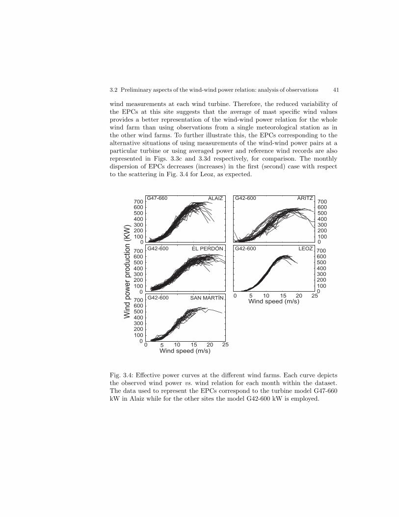
3.2 Preliminary aspects of the wind-wind power relation: analysis of observations 41

wind measurements at each wind turbine. Therefore, the reduced variability ofthe EPCs at this site suggests that the average of mast specific wind valuesprovides a better representation of the wind-wind power relation for the wholewind farm than using observations from a single meteorological station as inthe other wind farms. To further illustrate this, the EPCs corresponding to thealternative situations of using measurements of the wind-wind power pairs at aparticular turbine or using averaged power and reference wind records are alsorepresented in Figs. 3.3c and 3.3d respectively, for comparison. The monthlydispersion of EPCs decreases (increases) in the first (second) case with respectto the scattering in Fig. 3.4 for Leoz, as expected.

Fig. 3.4: Effective power curves at the different wind farms. Each curve depictsthe observed wind power vs. wind relation for each month within the dataset.The data used to represent the EPCs correspond to the turbine model G47-660kW in Alaiz while for the other sites the model G42-600 kW is employed.

42 3 The influence of the Weibull assumption in monthly wind energy estimation

The total monthly mean wE (wE) and its corresponding standard deviation(Sm) are indicated in the second column of Table 2.2. The final total productiondepends on the balance between the number of wind turbines available (see Table2.1) and the rated power. The maximum monthly energy production is achieved inAlaiz, where the most powerful turbines of the type G47-660 kW, are installed.Aritz is the location with less energy production stemming both from a lowerrated power and fewer turbines.

Correlations between the monthly power production series corresponding tothe different turbine models are larger than 0.9 at El Perdon, Leoz and SanMartın. For this reason, results concerning only one type of turbine (G42-600kW) will be shown in the three sites for simplicity from here on.

3.3 Methodology

The approach used to estimate monthly wE production is based on the useof the hourly frequency distribution of wind velocity within each month and anestimate of the power production dependence on wind, based, for instance, on thetheoretical power curve or some substitute of it obtained from the observations(Celik, 2004, 2003b,c).

An estimation of the total monthly wind energy (wE) production can beobtained from summing all the power contributions from the various wind classesconsidering their frequency of occurrence and scaling the sum to the total numberof time steps and turbines in the farm:

wE = ∆tNNt

n∑

i=1

pout(wi)f(wi), (3.1)

where f(wi) is the expected frequency for each of the n wind speed class intervalsrepresented by wi and pout(wi) is a transfer function for the wind power vs. windrelationship that provides an estimation of the power production for a given wi;∆t is the time resolution of the input wind speed data (1 hour), N is the totalnumber of hours per month and Nt is the number of wind turbines. In thosewind farms with several types of turbines installed, Eq. (3.1) is computed foreach group of wind turbines, with different pout(wi) and Nt and the results aresummed to provide a single estimation for the whole wind farm. Consequently,this method produces a cumulative contribution of the frequency of wind in eachinterval to the total wind power production by multiplying the frequency termsby the corresponding power contribution of each bin, pout(wi). Many practicalcases involve situations in which wE must be estimated without knowing theprecise wind frequency distribution, f(wi), or the exact wind power vs. wind

3.3 Methodology 43

relation, pout(wi). In such cases, two potential sources of error are involved in thewE estimation through Eq. (3.1): one stems from the use of an approximationfor pout(wi), for instance if the theoretical/manufacturer power curve is used(Akpinar and Akpinar, 2005a; Seguro and Lambert, 2000); the other is associatedwith the use of a theoretical distribution for f(wi) (Ramırez and Carta, 2006;Pryor and Schoof, 2005; Li and Li, 2005a).

As previously mentioned, the use of an approximation for pout(wi) introducesan error related to the fact that the power curve itself is an approach to themore complex actual wind-wind power relation (see Fig. 3.2) which also varieswith time (e.g. Fig. 3.4). Due to factors such as turbulence, the effect of windvelocity reduction caused by the shadow between turbines, the variability ofwind direction, etc., the actual power production does not coincide exactly withwhat theoretical power curves predict. Furthermore, the use of a global (spatiallyaveraged in this work) power curve also introduces perturbations with respectto the expected power production since the wind power generation from eachindividual wind turbine within the site is not identical to the rest (Noorgardand Holttinen, 2004). The use of a theoretical probability distribution insteadof the observed wind velocity frequency involves an additional source of errorwhen estimating wE in Eq. (3.1) as much as the specific wind speed frequencydistribution of a certain month deviates from the shape of the assumed theoreticalprobability distribution function.

This chapter is devoted to explore the second source of error through eval-uating the extent to which the assumption of a given probability distribution,f(wi), can contribute to the error in the final monthly wE estimation. A com-plete evaluation of errors involves analyzing the impacts of selecting a certainpout(wi) power curve. Thus, some of the results obtained herein do have implica-tions concerning the effect of the pout(wi) and this source of error will be subjectof attention in Chapter 4.

The Weibull probability distribution has been selected for this study in thebasis of the arguments provided in Section 3.1. A limitation of the Weibull densityfunction is that it can not estimate with accuracy the probability of calms orvery low wind velocities (Weisser and Foxon, 2003). However, this aspect doesnot produce a considerable impact on the final wE estimation as, for the lowestwind intervals, there is no relevant contribution to the wind power production, i.e., the corresponding pout(wi) is negligible in comparison to the power associatedwith the largest wind velocities, see for instance the values in Figs. 3.2 and Fig.3.4 for low wind speeds. For wind velocities below 4 ms−1 the production is 0kW and for wind speeds smaller than 6 ms−1 the power output is under 100 kW.Though the selection of a particular probability distribution such as the Weibullcan inevitably narrow the final conclusions to the specific case studies in which

44 3 The influence of the Weibull assumption in monthly wind energy estimation

this distribution is used, the following sections will arrive at some implicationswhich attain a broader focus.

The evaluation of the error contribution from the probability terms f(wi) canbe easily done through establishing a maximum benchmark level of predictabilitywith respect to which other errors can be defined. Of all possibilities, the mostaccurate estimation of wE with Eq. (3.1), would be the one obtained by usingthe observed frequency histogram in each specific month as f(wi) and the ob-served wind power vs. wind relation as pout(wi), within each particular month.The variability in the actual monthly frequency distributions and effective powercurves is shown in Figs. 2.2 and 3.4. Such an estimation serves as the mostaccurate estimation possible and therefore as a benchmark of the upper limit ofpredictability that can be obtained using Eq. (3.1). This estimate will be denotedas wEH−ref . The error made by this estimation is obtained by calculating thedifference between wEH−ref and the observed wE (wEobs), and will be denotedas

ξ1 = wEobs − wEH−ref (3.2)

This quantity provides information about the error in the method described byEq. (3.1), independent on any assumption made on pout(wi) and f(wi). This erroris derived from the extent to which the EPC is a bad representation of the windpower vs. wind relation in the different masts and from the approximation whichimplies considering a frequency histogram. If, in a limit case, the wind power vs.wind transfer function was perfect, when using point values, the estimated andobserved wE would converge.

The second control estimation calculated also assumed the correspondingEPC for each month as pout(wi), but in this case, the theoretical Weibull fre-quencies were employed as f(wi) in Eq. (3.1). This estimation is denoted aswEH−EPCw. As wEH−ref and wEH−EPCw only differ in the use of the Weibullexpected frequencies in one case and the observed ones in the other, the contri-bution to the error of the frequency terms, under the assumption of a Weibulldistribution can be studied from the difference between both previous estima-tions,

ξ2 = wEH−ref − wEH−EPCw (3.3)

= ∆tNNt

n∑

i=1

pout(wi)fobs(wi) − ∆tNNt

n∑

i=1

pout(wi)fweib(wi)

= ∆tNNt

n∑

i=1

pout(wi) [fobs(wi) − fweib(wi)] ,

3.3 Methodology 45

This should help to understand qualitatively and quantitatively the effect thatdiscrepancies between the observed and the expected Weibull frequencies producein the monthly wE estimation at the locations considered. A third error thataddresses the combined effect of both kinds of error described above is providedby

ξ3 = wEobs − wEH−EPCw (3.4)

This magnitude incorporates the effects of assuming a certain probability functionto the method errors in ξ1.

3.3.1 Fitting to the Weibull probability distribution

The Weibull probability density function (Justus et al., 1977; Takle and Brown,1978),

f(w) =k

c

(w

c

)k−1

exp

[

−(w

c

)k]

, (3.5)

where w is the wind speed, is defined by two parameters, k and c. k is the dimen-sionless shape parameter related to the variability of wind and therefore, providesan approximation of the flatness of the distribution. c is the scale parameter inms−1, and is related to the mean value of the distribution (Perez et al., 2007).In this work, both parameters defining the Weibull function are calculated usingthe method of moments, which provides a suitable estimation of the parameters(Fawzan, 2000; Seguro and Lambert, 2000; Gove, 2003) and the best result forthe higher wind speed values in the distribution according to Tuller and Brett(1984). This method is based on the calculation of the first n sample momentsand the use of them as estimators of population parameters of the distribution.The mean Weibull parameters, calculated over the whole period of data, andtheir corresponding standard deviations are summarized in Table 3.1 (columns3 to 4). The overall values of the shape parameter distribute close to the valuek = 2, typical in practice (Biswas et al., 1990) and the limit value in which theWeibull distribution reverts to the Rayleigh distribution. The deviation of k islarger at Aritz and El Perdon, an unsurprising feature in view of the variabilityof the monthly distributions (points) in Fig. 2.2 and the wind speed standarddeviation values in Table 2.2. The scale parameter (c) provides larger values forAritz and El Perdon, the sites with maximum wind speed; deviations for thisparameter are also larger at these sites.

The goodness of fit of the Weibull adjusted distributions to the observed datawas established in terms of the χ2 statistic. This allows to test the null hypothesis

46 3 The influence of the Weibull assumption in monthly wind energy estimation

Table 3.1: Mean Weibull parameters (k, c), monthly mean estimations using theobserved histograms (wEH−ref ) and estimations using the Weibull histograms(wEH−EPCw) and their respective standard deviations (Sk, Sc, SwEH−ref

,SwEH−EP Cw

) at each wind farm.

k ± sk c ± sc wEH−ref (SwEH−ref) wEH−EPCw (SwEH−EP Cw

)

(adim.) (ms−1) (GWh) (GWh)

Alaiz 2.0 ± 0.3 9.0 ± 1.3 3.4 (0.8) 3.2 (0.8)Aritz 2.1 ± 0.5 9.4 ± 2.1 2.0 (0.8) 2.0 (0.8)El Perdon 2.4 ± 0.4 11.4 ± 1.5 3.2 (0.6) 3.1 (0.5)Leoz 2.1 ± 0.2 8.9 ± 1.0 2.2 (0.5) 2.0 (0.4)San Martın 2.5 ± 0.2 9.1 ± 1.2 2.8 (0.7) 2.8 (0.7)

that the actual sampled data follow a Weibull function (Akpinar and Akpinar,2005b; Dorvlo, 2002). The test statistic is defined as:

χ2 =n

∑

i=1

[O(wi) − E(wi)]2

E(wi)= N

n∑

i=1

[fobs(wi) − fweib(wi)]2

fweib(wi), (3.6)

with O(wi) and fobs(wi) being the absolute and relative observed frequenciesfor interval i, E(wi) and fweib(wi) the absolute and relative expected Weibullfrequencies for the same interval and N the total number of observations. Thepresence of the expected frequency in the denominator in Eq. (3.6) attempts toweight the squared differences between frequencies eliminating the dependenceon the specific shape of the distribution. That is, with the expected Weibullfrequency in the denominator all intervals have the same weight in the calculationof differences. χ2 will be used in the next section to analyze the goodness of fit andto illustrate its relationship with the error in the total monthly wE estimation.

One further comment is needed to address the sensitivity of χ2 test to thenumber of intervals and the existence of missing data. χ2 is sensitive to the choiceof the number of intervals to calculate histograms and differences in Eq. (3.6).Also Eq. (3.6) is sensitive to small frequency numbers in fweib(wi) which areoften related to the handling of the wind intervals at the tails of the distribution.In order to mitigate this problem, the same conditions were imposed to eachmonthly histogram, that is, the number of intervals were fixed and the tails ofthe distribution were forced to contain 3% of the data. The question whetherthe selection of a specific number of intervals may affect the conclusions met bythe analysis of the goodness of fit can be assessed by exploring the sensitivityof the χ2 values to a varying number of intervals. This is calculated at Leoz as

3.4 Analysis of results 47

an example and represented in Fig. 3.5. Monthly χ2 tend to slightly increaseas the number of intervals increases, although the variability of the time seriesis similar for all cases explored (Fig. 3.5a). This could lead to a situation inwhich the Weibull null hypothesis may be accepted or rejected, depending on theselection of the number of intervals selected, for some months. Nevertheless, fromFig. 3.5b it can be said that as the number of intervals increases, and so doesthe mean χ2 value, the critical value increases accordingly, pointing out that if nis kept constant the number of months that verify the Weibull assumption doesnot change significantly regardless of the specific value selected for n.

The presence of a varying number of missing data in each month would alsoaffect the results in Eq. (3.6). This could make it difficult to discriminate whetherchanges in χ2 correspond to a feature of the methodology or to the varying num-ber of observations in each monthly sample, which could plausibly influence theresulting values obtained in Eq. (3.6). Additionally, final monthly estimations ofwE in Eq. (3.1) could be affected by the lack of data at certain months whichcould lead to an inaccurate result when computing contributions from the avail-able hourly data. This possible perturbation was avoided by randomly selectinga fixed number of 350 hours (ca. 50% of observations in each month) from theavailable wind-wind power pairs for each month (see section 2.2). This number,as commented in the previous section, represents a balanced decision betweenusing months with a very low number of observations, which might not ade-quately represent the monthly means and totals and alternatively, selecting onlymonths with a high number of measurements, which would lead to a scarcenessof monthly records in original the data set.

3.4 Analysis of results

This section compares the observed and calculated monthly wind energies at thefive sites and analyzes the implications of using a Weibull probability function tomodel wind behavior. Section 3.4.1 presents the errors associated with the use ofEq. (3.1) and evaluates the impact of using the Weibull probability distributionon the energy estimations in terms of the behavior of the errors at each site alongthe period of observation. Section 3.4.2 explores the relation of the error termswith the quality of the fit through illustrating and discussing systematic biasesin the Weibull fit at the various sites.

3.4.1 Errors in wE estimation

The time evolution of the observed total monthly wind energy (wEobs) is com-pared to the resulting wEH−ref and wEH−EPCw estimations in Fig. 3.6 for

48 3 The influence of the Weibull assumption in monthly wind energy estimation

01/02

01/07

01/12

02/05

02/10

03/03

Time (year/month)

12 14 15 17 20 22 24

50

100

150

0

c2

Mean

c2

Critic

al

valu

ec

2

n intervalso

Mean c2

Critical c2

a)

b)

12 14 16 18 20 22 2420

24

28

32

36

40

44

48

52

56

60

64

Fig. 3.5: Sensitivity of the χ2 to the number of intervals considered in the goodnessof fit test at Leoz. a) χ2 time series as a function of the the different number ofintervals (see legend), b) Mean χ2 and critical χ2 value depending on the numberof intervals.

all wind farms. The mean values of the two estimated series (wEH−ref andwEH−EPCw) are shown in Table 3.1 (columns 5 and 6) for all locations. Both es-timations are close to the monthly mean observed value (second column in Table2.2). Fig. 3.6 shows that there is a general agreement between measurements andestimations in all cases analyzed. The estimations using a realistic power curveand actual monthly frequency histograms (wEH−ref ) are difficult to distinguishfrom the observational values (wEobs). Substituting the frequency histograms bythe Weibull approximation introduces a slight error that becomes obvious only

3.4 Analysis of results 49

at Leoz, i.e., the largest error is found in Leoz for the wEH−EPCw estimationwhich on average is no greater than 227 MWh (10.3%). It is interesting to notethat wEobs displays a considerable amount of intra annual and inter annual vari-ability which wEH−ref and wEH−EPCw are able to capture. Such variability inenergy production is likely related to changes in atmospheric circulation and willbe dealt with in Chapter 6. As expected from the wind energy production meansand standard deviations shown in Table 3.1, Alaiz and El Perdon are the sitesreaching higher energy productions in Fig 3.6.

wEH-ref

wEH-ref

wEH-ref

wEH-ref

wEH-ref

wEH-EPCw

wEH-EPCw

wEH-EPCw

wEH-EPCw

wEH-EPCw

Fig. 3.6: Total monthly observed wind energy (wEobs) and estimations (wEH−ref

and wEH−EPCw) at each site.

50 3 The influence of the Weibull assumption in monthly wind energy estimation

The monthly evolution of the three types of error, ξ1, ξ2 and ξ3 in the fivewind farms, is presented in Fig. 3.7 and allows for some further insight into theerror behavior. The errors are expressed in relative terms and they are the resultof the division of the average total error by wEobs in the case of ξ1 and ξ3 andby wEH−ref in the case of ξ2. It can be observed from Fig. 3.7 that most errorsare positive, thus suggesting some bias to underestimate wEobs. Celik (2003b)and Biswas et al. (1990) report results showing a tendency of the Weibull energyestimation to underestimate the reference energy in similar approaches. A sum-mary with the averaged errors for the whole period at each site is given in Table3.2. The smallest mean error corresponds to ξ1 (wEobs-wEH−ref ) at the threeof sites (Alaiz, El Perdon and Leoz) and to ξ2 (wEH−ref -wEH−EPCw) at Aritzand San Martın. Thus, the substitution of the empirical histogram by a fitteddistribution does not necessarily lead to larger errors in the energy estimationin spite of introducing additional errors in the probability representation. Thisfeature is also apparent in the time evolution of errors in Fig. 3.7. Though thismight appear counter intuitive at first sight, it stems simply from Eq. (3.1) andwill be discussed in the next section.

Table 3.2: Averaged relative (total) errors in monthly wE estimation at each windfarm (columns 1 to 3), average χ2 values (column 4) and correlations (r) betweenξ2 and χ2 time series at each wind farm (column 5). Columns 6 and 7 showcorrelations between errors and χ2 for the wind intervals where the contributionto Npout(wi) [fobs(wi) − fweib(wi)] is negative (ξ−2 ) and positive (ξ+

2 ) (see textfor details).

ξ1 ξ2 ξ3 χ2 r(ξ2,χ2) r(ξ−2 ,χ2) r(ξ+

2 ,χ2)

%(GWh) %(GWh) %(GWh)

Alaiz 2.6 (0.1) 4.5 (0.2) 7.2 (0.2) 34.8 0.3 -0.5 0.5Aritz 5.0 (0.1) 0.2 (4.10−3) 5.2 (0.1) 48.4 0.2 -0.5 0.6El Perdon 1.7 (5.10−2) 2.4 (0.1) 4.2 (0.1) 36.8 0.5 -0.5 0.6Leoz 0.9 (2.10−2) 10.3 (0.2) 11.3 (0.2) 55.0 0.6 -0.6 0.7San Martın 2.9 (0.1) 0.3 (0.01) 3.0 (0.1) 29.2 -0.2 0.2 -0.2

The largest impact of introducing the Weibull approximations is found at Leozwhere mean relative differences between wEH−ref and wEH−EPCw amount to10.3% (see Table 3.2). These larger differences are also apparent in Fig. 3.7. In-terestingly, the ξ1 methodological errors at Leoz are considerably smaller than atthe other sites, a feature that probably relates to the lower amount of variability

3.4 Analysis of results 51

x3 x3

x3x3

x3

Fig. 3.7: Time series of monthly errors (ξ1, ξ2, ξ3) in wind energy estimation ateach site.

in the wind power vs. wind relation at this location (see Figs. 3.2 and 3.4), wherea spatially averaged wind time series was computed from every wind turbine.

A last comment can be made concerning the behavior of the ξ3 errors whichbasically accumulate the ξ1 errors inherent to the method and ξ2 related toincorporating a theoretical distribution function as a substitute for the observedhistogram. As a result, changes with time in ξ3 (Fig. 3.7) are coherent with thosein ξ1 and ξ2 depending on which one has the largest contribution to the error.

52 3 The influence of the Weibull assumption in monthly wind energy estimation

3.4.2 Goodness of fit

The ξ2 errors shown in Fig. 3.7 represent a relatively small part of the variabil-ity in wEobs except for Leoz where they stand out amounting to about 10% onaverage. Even if the impact of a priori introducing the Weibull distribution as-sumption is relatively small, the associated errors still represent a considerableamount of energy and it is interesting to elucidate the reasons for such errorsand the potential contribution of the goodness of the fit to them. In addition, itcannot be ruled out that, for other sites not considered here, such contributionsmay be larger, thus it is relevant to understand the role of the frequency termsin Eq. (3.3). For this reason, the error contribution of the Weibull distributionwas evaluated through an exploratory analysis of the relation between ξ2 and themonthly evolution of the goodness of the fit by means of the χ2 statistic.

Table 3.2 (column 4) shows the average of all monthly χ2 values at eachsite and Fig. 3.8 compares the monthly evolution of ξ2 and χ2 along the periodof observation. The χ2

0.01,14 critical value, beyond which the null hypothesis isrejected for a 0.01% significance level and 14 degrees of freedom (the analysisuses 17 intervals for every month and 2 fixed parameters, k and c), is also shown.χ2 averages in Table 3.2 show the lowest values for San Martın and the largestones for Leoz in agreement with the relatively small ξ2 values in Table 3.2 andFig. 3.7 for both sites. It is interesting to note though, that Aritz shows a verylow ξ2 while it displays a comparatively large χ2. This suggests there is not aclose correspondence between smaller (larger) ξ2 and smaller (larger) χ2. Fig. 3.8allows for the assessment of this relation at a monthly resolution, studying thetime series of χ2 in comparison with ξ2. The amount of months that satisfy thenull hypothesis is variable from site to site. Though most of the months withavailable data at all sites register relatively low χ2, close to or lower than thecritical value, the percentage of months strictly respecting the threshold levelis smaller, e.g. at Alaiz, El Perdon and San Martın, 29%, 33% and 60% of themonths (respectively) show χ2 values that strictly suggest a Weibull distributionand at Aritz and Leoz lower percentages of 2% and 14% are registered. Thus,according to this test, the initial assumption of using a Weibull distribution isnot broadly met at all sites and time steps. To a large extent, San Martın can beconsidered Weibull distributed or very close to the Weibull distribution in mostmonths, but this assumption is only partially substantiated at the other sites. Inspite of this, the replication of the energy production is reasonable in Fig. 3.6 aspreviously illustrated. As it was argued before, the poorer quality of the fit alongthe period of observation at Leoz is consistent with the high ξ2. However, thislink between larger (smaller) errors and worse (better) fit is not evident at everysite and time step.

3.4 Analysis of results 53

Fig. 3.8: Time series of ξ2 errors and monthly values of χ2 at each site.

The temporal variability in χ2 and ξ2 at Leoz reveals coherent changes thatlead to a correlation of 0.6 linking larger (smaller) distribution errors to larger(smaller) energy errors. Correlations for the other sites are shown in Table 3.2(column 5) with values of 0.3 at Alaiz and 0.5 at El Perdon and negligible values(0.2) at the remaining sites. Thus, some of the sites show some consistent tem-poral link between χ2 and ξ2, however, as it was argued on the basis of Table3.2 above, larger (smaller) ξ2 do not regularly coincide with larger (smaller) ξ2

values suggesting that a closer Weibull fit does not guarantee smaller ξ2 errors.For instance if the time series at Aritz is considered, May and June of year 2000show respectively a low and a high χ2 value that meets in the first case thecritical level and considerably departs from it in the second, while at the same

54 3 The influence of the Weibull assumption in monthly wind energy estimation

time similar ξ2 values are attained for both months; such type of events are notinfrequent through the time series in Fig. 3.8. The reasons for this behavior canbe found on the error contributions by the [fobs(wi) − fweib(wi)] terms in Eq.(3.3).

Fig. 3.9 illustrates the quality of the Weibull fit for various χ2 levels and pro-vides some insight into their contribution to Eq. 3.3. Two examples of histogramsand associated Weibull fits for low and relatively large χ2 values at Alaiz andLeoz are. The selected months were arbitrarily chosen to be December 2001 andJuly 2002. For December 2001 deviations of the observed histogram from theWeibull shape produce χ2 values of 19 (Alaiz) and 22 (Leoz). Larger deviationsfrom the Weibull shape in July 2002 generate χ2 values of 72 (Alaiz) and 95(Leoz).

Fig. 3.9: Absolute frequency histograms (bars) and adjusted Weibull probabilityfunctions (scaled to absolute frequencies) for December 2001 and July 2001 atAlaiz and Leoz. χ2 values are indicated for each case.

The larger differences contributing to the error in July are due to the Weibullfunction overestimating the observed histogram in the intermediate range of windvalues and underestimating it in the lower and upper ranges. These discrepancies

3.4 Analysis of results 55

between the observed and adjusted distribution seem to often present a similarpattern of over- (under-) estimation in the intermediate (lower and upper) windranges, i. e. negative (positive) values of the [fobs(wi) − fweib(wi)] terms in Eq.(3.3). In order to illustrate this deformation in the observed histogram a disper-sion diagram in which points represent the differences in absolute frequencies,N [fobs(wi) − fweib(wi)] (observed minus expected absolute frequencies), for allintervals, in every month within the specific wind farm, is represented in Fig. 3.10,together with the line representing the average of all points. It can be appreci-ated that there is a tendency to under- (over-) estimate the Weibull frequencyvalues in the lower and upper (middle) range of wind speeds, generating positive(negative) results in N [fobs(wi) − fweib(wi)]. This produces therefore positive(negative) contributions in Eq. (3.3) as it is the difference fobs(wi) − fweib(wi)that imposes the sign to the error contribution in ξ2=wEH−ref -wEH−EPCw.

This underestimation (overestimation) is more pronounced at Leoz and it isless noticeable at San Martın and Aritz. At Alaiz and El Perdon such deforma-tion is also apparent in the experimental histogram. The error contributions ofdifferent sign tend, therefore, to be systematic in Fig. 3.10 and can be partiallyaveraged out in Eq. (3.3). Thus in spite of having relatively large differencesbetween the theoretical and actual frequency histogram, the impact of themcan be at least partially balanced out by their sign, producing relatively smallcontributions in Figs. 3.6 and 3.7. Additionally, the differences between bothdistributions are weighted by the factor, pout(wi) in Eq. (3.3). The most sig-nificant production of wE corresponds to the upper intervals of the histogram,that is, to the higher wind speed values, where the power generation is nearlythe rated power (Fig. 3.2). Thus, the weight applied by the factor pout(wi) isconsiderably greater for these intervals than for the rest. This makes their contri-bution to the errors larger. A dispersion diagram representing all the products,Npout(wi) [fobs(wi) − fweib(wi)] is presented in Fig. 3.11. It shows that theseproducts are negligible in the lower range of wind speeds as the energy producedhere is also small. In the upper (intermediate) range of wind values the net con-tribution of the products in Eq. (3.3) becomes positive (negative) as shown inFig. 3.10. As the contribution to the error is larger for the upper range of windspeeds, the dominant effect is a positive error in ξ2=wEH−ref -wEH−EPCw andthus an underestimation of the actual energy production as observed in Fig. 3.6and 3.7 and Table 3.1 (see subsection 3.4.1). The underestimation is larger forthe sites where the positive contribution of the upper range of wind speeds islarger in comparison to that of the intermediate speeds. This is the case for Leoz,Alaiz and El Perdon, the sites that displayed larger ξ2 averages in Table 3.2.Therefore, a larger level of underestimation of the monthly wEobs is related to

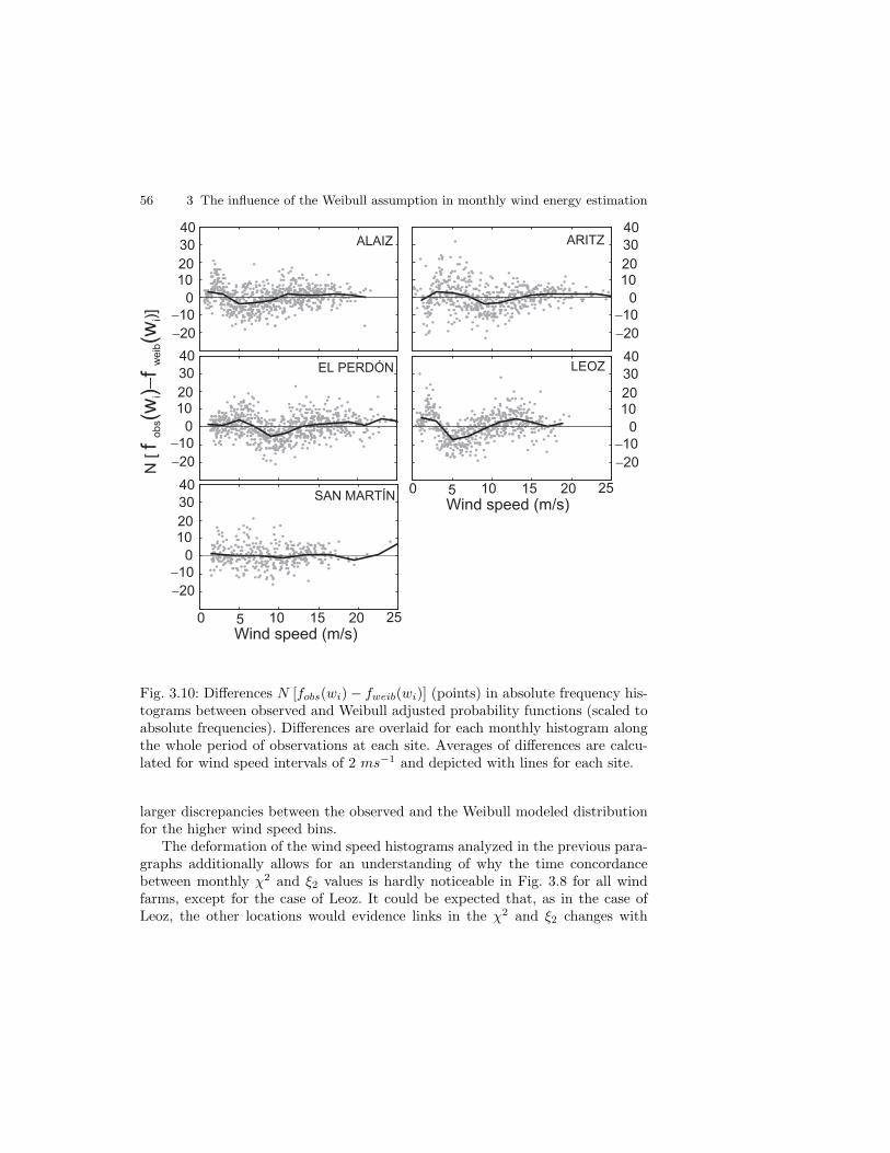
56 3 The influence of the Weibull assumption in monthly wind energy estimation

Fig. 3.10: Differences N [fobs(wi) − fweib(wi)] (points) in absolute frequency his-tograms between observed and Weibull adjusted probability functions (scaled toabsolute frequencies). Differences are overlaid for each monthly histogram alongthe whole period of observations at each site. Averages of differences are calcu-lated for wind speed intervals of 2 ms−1 and depicted with lines for each site.

larger discrepancies between the observed and the Weibull modeled distributionfor the higher wind speed bins.

The deformation of the wind speed histograms analyzed in the previous para-graphs additionally allows for an understanding of why the time concordancebetween monthly χ2 and ξ2 values is hardly noticeable in Fig. 3.8 for all windfarms, except for the case of Leoz. It could be expected that, as in the case ofLeoz, the other locations would evidence links in the χ2 and ξ2 changes with

3.4 Analysis of results 57

Fig. 3.11: As in Fig. 3.10 but for the terms Npout(wi) [fobs(wi) − fweib(wi)].

time. The lack of this clear relation can be easily understood if it is recalled thatthe differences between observed and Weibull frequencies, fobs(wi) − fweib(wi),take part in Eqs. (3.3) and (3.6) in a different way. While in their contributionto χ2 is always positive, in ξ2 positive or negative resulting differences can par-tially cancel their respective contributions. Therefore, it is possible that smallξ2 values are associated with large χ2 values. This fact disguises the expectedrelation between χ2 and ξ2. Alternatively, small χ2 values would be indicative ofsmall frequency differences, but can contribute to the final ξ2 value differentlydepending on the w range they are produced at and on the pout(wi) factor thatrelatively amplifies or attenuates them.

58 3 The influence of the Weibull assumption in monthly wind energy estimation

The absence of concordance between χ2 and ξ2, i. e. the partial cancellationof error, would be lessened if the differences fobs(wi) − fweib(wi) were mainlypositive or mainly negative, that is, if there was a dominant sign in the interme-diate, and preferably, in the upper intervals of wind speed, where the productionof wP is larger. That is the case of Leoz (Figs. 3.10 and 3.11) where the highestcorrelations were found (0.6) between χ2 and ξ2. Alternatively, the three bandsin which Fig. 3.10 and 3.11 conceptually divide the range of wind speed can beconsidered separately and compared with χ2, the rationale being the fact thatthe underestimation and overestimation discrepancies between monthly observedand Weibull adjusted histograms take place in a related way, i.e., the larger un-derestimation in the lower and upper bands, the larger the overestimation in theintermediate band. This can be argued on the basis that the sum over all relativefrequencies is 1, thus, if the probability of occurrence in the Weibull histogram islower than the observed frequency at the intermediate frequencies, the probabili-ties in the lower and upper wind ranges must necessarily be larger. Therefore, theξ2 errors accumulated within the bands generating positive contributions (lowerand upper) and that producing negative contributions (intermediate) in Eq. 3.3should behave coherently with time and display a more obvious relation respec-tively with χ2 than the total ξ2 added contributions in Eq. (3.3). In order toillustrate this, the positive (negative) error contributions were computed usingas boundaries the wind speed intercepts with the axis of the averages lines ateach site in Fig. 3.11. The resulting errors were denoted as ξ+

2 (ξ−2 ) and plottedfor comparison in Fig. 3.12. These quantities verify that ξ2=ξ+

2 +ξ−2 . Their evo-lution in Fig. 3.12 shows a much more consistent behavior with changes in χ2 ashighlighted by the correlations values show in Table 3.2 (columns 6 and 7). Theimproved correlations with the different sign error contributions relative to thosewith the total ξ2 (column 5 in Table 3.2) highlight the fact that the lack of a clearassociation between χ2 and ξ2 in Fig. 3.8 stems from the partial cancellation oferrors of different sign (ξ+

2 vs. ξ−2 ). In fact, Fig. 3.12 allows for the discriminationof the dominant error contribution at each time step that justifies the occurrenceof a large χ2 value.

3.5 Conclusions

This work compared observed and estimated monthly wind energies. Observa-tions were based on hourly wind velocity and wind power production measure-ments at five wind farms in the Northeast of the IP (Fig. 2.1).

As a first approach to the estimation of wind energy the best available in-formation for the wind power vs. wind relation and for the frequency histogramwas considered for each month. This served as a means of quantification of the

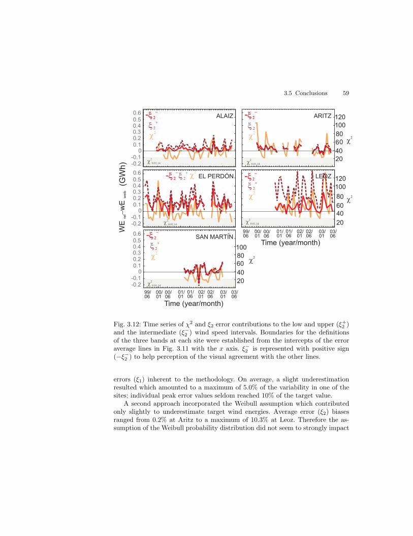
3.5 Conclusions 59

Fig. 3.12: Time series of χ2 and ξ2 error contributions to the low and upper (ξ+

2 )and the intermediate (ξ−2 ) wind speed intervals. Boundaries for the definitionsof the three bands at each site were established from the intercepts of the erroraverage lines in Fig. 3.11 with the x axis. ξ−2 is represented with positive sign(−ξ−2 ) to help perception of the visual agreement with the other lines.

errors (ξ1) inherent to the methodology. On average, a slight underestimationresulted which amounted to a maximum of 5.0% of the variability in one of thesites; individual peak error values seldom reached 10% of the target value.

A second approach incorporated the Weibull assumption which contributedonly slightly to underestimate target wind energies. Average error (ξ2) biasesranged from 0.2% at Aritz to a maximum of 10.3% at Leoz. Therefore the as-sumption of the Weibull probability distribution did not seem to strongly impact

60 3 The influence of the Weibull assumption in monthly wind energy estimation

the energy calculation. The reasons for this were not found to be based on abroad high quality of the Weibull fit but on a partial cancellation of error termsin the wind energy calculation.

An analysis of the goodness of the fit to the Weibull distribution based onthe χ2 statistic enabled an exploration of the relation between the quality ofthe wind speed fit and the discrepancies between observed and estimated windenergy. Such analysis revealed that the Weibull assumption could not be broadlysubstantiated at all the sites: the representativeness of the Weibull distributionvaried from site to site and from month to month.

The relation observed between the χ2 statistic and the estimated errors sug-gested that months which can not be strictly considered to be Weibull distributeddo not necessarily present higher errors in the wind energy estimation. The lackof an obvious relation between the error and the χ2 statistic is due to partialcancellations of opposite sign contributions to the error in the calculation of themonthly energy which do not take place in the χ2 computation.

The error contributions to the energy calculation and to the χ2 statisticrevealed that the Weibull distribution tends to overestimate the observed his-tograms in the intermediate wind speed range and to systematically underesti-mate it in the lower and higher wind speed intervals. The effects of these depar-tures from the observed frequency histogram tend to be averaged out due to thedifferences of sign. However the product by the power terms in the calculationof wind energy weights more over the highest wind speeds, thus underestimationerrors in this range tend to dominate and contribute to the systematic observedbias to underestimate total wind energy. It could be expected that sites/monthswith larger underestimations in the highest wind speed intervals disclose a muchmore evident relation between the energy estimation error and the performanceof the Weibull probability distribution as it is the case of Leoz.

The next chapter is devoted to examine the contribution of the power termsto the errors in the wind energy estimates (Eq. 3.1).

4

A comparison of methodologies for monthly wind

energy estimation∗

In the previous chapter the agreement between empirical and theoretical windspeed probability distributions was analysed, together with an evaluation of theimpacts of assuming a particular theoretical wind PDF on the estimation ofmonthly wind energy. In the present chapter the effect of selecting certain trans-fer functions between the wind speed and the wind power is explored. Withthis aim, monthly wind energy estimations obtained by means of three differentmethodologies are evaluated. One of the approaches is based on the combinedcontribution of the hourly wind speed frequency distribution and the correspond-ing power production. Several alternatives to represent the empirical wind powervs. wind speed relationship are considered in this context and their impacts on theerror of monthly energy estimations assessed. Two more approaches are used toderive monthly energy estimates directly from monthly wind values: one uses thetheoretical power curve to obtain interpolated monthly wind power productionvalues and the other consists in a simple linear regression between the observedwind speed and wind power monthly pairs, which serves as an approximation tothe global power curve. It will be shown that linearity is a reasonable assumptionfor the relation between wind speed and power production at monthly timescales.This result will have relevant implications for regional prediction of wind energyfrom atmospheric variables as it will prove useful in the identification of connec-tions between the wind power and the large scale circulation in Chapter 6, PartII of this thesis.

∗ The main contents of this chapter are included in:Garcıa-Bustamante, E., J. F. Gonzalez-Rouco, P. A. Jimenez, J. Navarro and J.P. Montavez, 2009: A Comparison of Methodologies for Monthly Wind EnergyEstimation. Wind Energ., 12, 640-659.

62 4 A comparison of methodologies for monthly wind energy estimation

This chapter is organized as follows. The next section underpins the rationalefor exploring the role of the wind-wind power relationship in the estimation oftotal monthly wind energy. Section 4.2 describes and comments on the approachesemployed to estimate wE from wind. Section 4.3 presents and discusses resultsand finally, main conclusions are summed up in section 4.4.

4.1 The rationale

The wind energy (wE) market (facilities, wind energy conversion systems, energypolicies, wind speed prediction, etc.) has experienced a fast and wide develop-ment in many regions of the globe, and some of them have been exploiting windresources since a few decades ago (Ackerman and Soder, 2002; Jager-Waldau andOssenbrink, 2004; Flowers and Dougherty, 2004; Kenisarin et al., 2006; Faulinet al., 2006; Fairless, 2007). Thus, admissibly long wE production series are nowavailable for many locations and it is possible to use them to accurately validatethe empirical relations between wind speed and power production at the varioustimescales of interest for resource assessments. For instance, in the previous chap-ter monthly wE was estimated at several wind farms in the Northeast of the IPassuming a theoretical PDF (Weibull) would fit hourly wind speed observations.Using such a technique, the frequency terms are weighted by the correspondingpower output, which can be derived from the TPC or some substitute of it. Inthat particular case, the study was focused on the evaluation of the magnitudeand nature of the error that the use of a Weibull distribution introduces in theestimation of monthly wind energy. This was done by using the historical recordsof power outputs to isolate the effects produced by the theoretical probability dis-tribution. Celik (2003b,c) employed measured wE values generated by a specifictype of wind turbine and hourly wind observations to fit a third order polyno-mial curve that attempts to depict an experimental power curve, alternatively tothe TPC. Availability of wE time series allows for a translation between windspeed and wE production for a specific site helping to understand the underly-ing relation between both variables at every timescale. Such a relation can beused for instance in the assessment of the sustainability and predictability ofwind resources (Weisser and Foxon, 2003; Jamil et al., 1995; Mathew et al., 2002;Bechrakis et al., 2004; Weisser, 2003).

The objective of this part of the work is to illustrate the performance of severalmethodologies in estimating monthly wE production. This is done in an attemptto review some typical approaches for estimating wind power from wind speedand in doing so, exploring and understanding the relation between wind speed anwind power production at monthly timescales. For this aim, wind speed and wEwind production data from five wind farms sited in Northeast IP (see Section 2.2)

4.2 Analysis of methodologies 63

are employed. Three methods are compared in their ability to estimate monthlywE (wEm). The first method examined is a common technique in wind resourceevaluation that involves the fit of hourly wind data to a theoretical PDF and theuse of a power curve that translates wind speed into wind power. The inspectionof this methodology can be regarded as a continuation of the previous chapterwhere the impact of errors in the wind speed PDF distribution was analyzed.Here the impact of selecting a specific power curve on the estimations and theassociated errors of wEm is included. This method operating in hourly timescalesis compared to other approaches that only use monthly resolution data. One ofthem adopts the strategy of estimating monthly wE by interpolating monthlywind speed values in the TPC. This rough approximation could be useful as abenchmark in the estimation of wEm in the case that no historical wE productiondata were available at a particular site. The last procedure is based on the em-pirical relationship found between wind speed and wind power at monthly timescales and consists in assuming a linear relationship between wEm and monthlywind velocity. Therefore, the standard approach providing estimations of wEm

from hourly wind speed is compared to even more parsimonious approximationsmaking use of coarser temporal monthly resolution information. This will allowfor evaluating to what extent situations in which only monthly data are availablecould involve a loss of information in the estimation of wEm.

4.2 Analysis of methodologies

Wind speed and wind power production data for the analyses herein were de-scribed in Section 2.2 and are the same as those used in the previous chapter.

Three strategies are compared in their performance to derive estimations ofwEm. The first strategy is based on a standard procedure (Celik, 2003c,b,a;Biswas et al., 1990; Celik, 2004) that takes into account hourly wind velocitydata. It considers the observed wind speed frequency histogram, or a viable fit toa theoretical PDF of the frequency terms, and a transfer function representingthe relation between wind speed and power production. The other two strate-gies lean on the use of monthly wind and power production data. The secondapproach is based on the very rough assumption that the TPC would be valid atmonthly timescales and thus, translates monthly wind values into monthly powerproduction through an interpolation in the TPC. Some considerations addressingthe validity of such an assumption are discussed in section 4.2.2.

The third approach is based on assuming that the relationship between windspeed and wind power is linear. Their monthly averages, as will be discussedin section 4.2.3 (e.g. Fig. 4.2) fall in the quasi-linear part of the TPC and aresuggestive of a simple linear empirical relationship between them.

64 4 A comparison of methodologies for monthly wind energy estimation

A more detailed description of the three methodologies is presented in thefollowing subsections.

4.2.1 Estimation based on hourly resolution data

The first approach to estimate the total production of wEm is based on the useof the hourly distribution of wind speed within each month and an estimateof the wind speed-wind power dependence such as the TPC or some substituteof it. This method has become relatively standard in obtaining wE estimatesfrom high temporal resolution wind speed series (Mathew et al., 2002; Bechrakiset al., 2004; Weisser, 2003; Pryor and Schoof, 2005) and allows to assess to whatextent including hourly information refines results in comparison with the otherapproaches described below that only consider monthly time resolution. Theestimation of the wEm is obtained through:

wEH = ∆tNNt

n∑

i=1

pout(wi)f(wi) (4.1)

(notation in Eq. 4.1 follows that of Eq. 3.1 in Chapter 3).Several comments can be made at this point concerning the evaluation of

f(wi) and pout(wi). As discussed in Section 3.3, of all possibilities, the mostprecise estimation of wE for a given month should be the one calculated usingthe observed wind speed frequency, f(wi), and the observed relationship betweenpower production and wind speed within each particular month, pout(wi). Thewind speed frequencies can be easily obtained from splitting the range of hourlywind observations into wind intervals, whereas the effective relationship betweenwind speed and generated power can be derived from the observation of the powerproduction at each one of those intervals. This provides an empirical wind powervs. wind speed curve that was denoted in Chapter 3 as the EPC and that can beused as pout(wi).

Such an estimation was already used in Chapter 3 as the reference estimation.There, as in this chapter, it represents a benchmark of the predictability that canbe obtained using the procedure explored in the previous chapter (Eq. 3.1) andthat here (Eq. 4.1) serves also to provide an idea of the systematic error inthe methodology associated with the discretization of the wind speed series intointervals. This estimate will be also denoted herein as wEH−ref .

As discussed in Chapter 3, many practical cases involve situations in whichthe precise knowledge of pout(wi) and f(wi) is not available. In these practicalsituations, wEH must be estimated by making approximations to the wind fre-quency distribution and the corresponding power output. A first approximationin such cases is the use of a specific theoretical PDF, like the Weibull function for

4.2 Analysis of methodologies 65

instance (Tuller and Brett, 1984; Palutikof et al., 1987; Celik, 2003b; Pryor andSchoof, 2005; Dorvlo, 2002) as a substitute for the observed wind speed frequency.This constitutes a first source of error when estimating wEH in Eq. (4.1) to theextent that the specific wind distribution of a certain month deviates from theWeibull shape; the deviation being particularly relevant in the high wind speedrange where the largest power production is achieved (recall results in Chapter3).

A second source of error stems from the assumptions made to estimatepout(wi). One of the goals in this chapter is the evaluation of the impact ofusing an approximation to the power terms in Eq. (4.1). With this purpose theobserved frequency distribution is employed to provide the f(wi) terms (as inthe case of wEH−ref ) and a set of variants for the power outputs terms wereconsidered in order to isolate their influence on the wEm estimations. These al-lows for the segregation of the two sources of error as previously done in Chapter3 but, in this case focused on the impact of the assumptions made about thepower curve. Thus, in addition to wEH−ref that provides information about themethodological error in Eq. (4.1), three more estimates of monthly energy pro-duction obtained with different versions of the wind speed-power relation areproposed here. The substitutes for the EPCs adopted herein are also consideredto be representative of the whole wind farm, in spite of the fact that power pro-duction may show changes within the group of wind turbines (Noorgard andHolttinen, 2004).

The first candidate for the pout(wi) terms is the TPC. This is the simplest androughest approximation since the TPC does not take into account the global windfarm effects (e.g shading between turbines). However, it has the advantage thathistorical data are not required. Bechrakis et al. (2004), Jaramillo and Borja(2004) and Bivona et al. (2003) for instance, have used commercial TPCs toobtain energy production. Hereafter the energy estimation produced using theTPC as an estimate of pout(wi) will be denoted as wEH−TPC .

Two more approximations of the EPC are considered: an average power curve(APC) and a third order polynomial fit curve (PFC). The APCs are calculated asthe average of all the EPCs along the period of observation at each site, calculat-ing for each wind speed interval the corresponding mean power production value.The PFC is the cubic polynomial that better fits the whole ensemble of EPCs.The use of these approximations is intended to explore the potential benefitsof developing more elaborated models as substitutes for the EPC and that canbe used as a realistic representation of the wind speed-wind power relationship.These approaches can incorporate some effects that are specific to the wind farmlocation and make use of the already existing information to face situations inwhich no data for a particular month are available. Even if these two new power

66 4 A comparison of methodologies for monthly wind energy estimation

curve models appear to be somewhat more elaborated than the EPC case, theyare still conceptually simple since they do not take into account the effects ofmore complicated features like the dependence on wind direction, the relativeposition of masts within a wind farm, air density, etc. This will be commentedon in Section 4.3.

In order to keep independence between monthly wEH estimations and theEPC averaging/fitting process through the methodological assessment, the datafor the target month (the month for which the wEH is going to be estimated)are excluded in the calculation of the APC/PFC curves. With this specification,a single APC/PFC is independently obtained for each particular month. Thisprocedure can be compared to a crossvalidation approach through which thetemporal robustness of the empirical relation found between sets of predictandand predictor variables is assessed (von Storch and Zwiers, 1999): for each timestep the estimation of the target-predictand variable (i.e., wind energy productionherein) is obtained from the available predictor (i.e., wind speed) through the useof an empirical model (in this case, APC or PFC) that is built on the basis ofthe available information from all other time steps. The energy estimation in thiscase is denoted with wEH−APC/wEH−PFC .

Fig. 4.1 illustrates the three approaches (TPC, APC, PFC) employed to repre-sent the pout(wi) terms in Eq. (4.1). December 2001 is shown as a particular caseexample. The TPC generally underestimates the power generated at the lowerwind speeds whereas it tends to overestimate it for the higher wind velocities.The weighting effect of the pout(wi) terms in Eq. (4.1) is stronger for the high-est wind speeds and thus, a global overestimation of the final wEH−TPC shouldbe expected. This point is further analyzed through the interpolation methodin Section 4.2.2. The APC and PFC are very similar, though the PFC displaysgenerally (not shown) smaller power values than the APC for the same wind.

The dispersion of the hourly wind speed-wind power pairs discussed in Section2.2 is also evidenced in the representation of the EPCs (Fig. 4.1). Such an effectis, as expected, minimized in Leoz where the set of EPCs displays a much smallermonthly variability. A consequence of the spatial average over the set of turbinesto obtain a single power production series at each wind farm can be appreciated inthe bended shape of some of the EPCs close to the cutoff wind part of the curve inFig. 4.1; for winds above the cutoff level, some turbines may be stopped leadingto a diminished average power production in the whole wind farm (for moredetails see Section 3.2). An alternative to the PFCs calculation adopted hereincould be the implementation of a polynomial fit over all the available hourlywind speed-wind power pairs (Celik, 2003b,a). However the large dispersion ofhourly observations leads to low signal to noise ratios that do not statisticallysupport the fit to polynomial functions of orders higher than one. The generation

4.2 Analysis of methodologies 67

Fig. 4.1: TPC, APC and PFC (see legends) for December 2001 at each of thewind farms; wind turbine types are G47-660 kW in Alaiz and G42-600 kW inAritz, Leoz and San Martın. In El Perdon no TPC was used (see text).

of monthly EPCs from hourly data enhances signal to noise ratios (Fig. 4.1) andallows for implementing higher polynomial orders that are consistent with thetypical shape of a TPC. The TPCs cannot be established properly for El Perdondue to the frequent technical manipulations during the period of measurementsand that probably contribute to a large dispersion of the wind speed-wind powerpairs at this specific wind farm. Thus, the corresponding curve for this site is notshown in Fig. 4.1.

The comparison of wEH−ref with the energy production calculated using thevarious estimates of the EPC (wEH−XXX , with XXX ≡ TPC, APC, PFC ) al-

68 4 A comparison of methodologies for monthly wind energy estimation

lows for an evaluation of the errors associated to the pout(wi) terms in Eq. (4.1).However, in order to compare the results of this approach to the ones describedin Sec. 4.2.2 and 4.2.3 it is desirable to provide an integral error estimation thatincludes also the effect of the f(wi) terms discussed above. The evaluation of theerror impact of the frequency terms is non trivial since it depends on the theo-retical PDF that wind speed is assumed to follow. For the sake of simplicity andconsistency with the previous chapter, this study adopts the Weibull distribu-tion. Therefore the f(wi) terms are substituted by their corresponding Weibullestimates following the same procedure as in Chapter 3. The monthly energyestimations including both types of error will be denoted as wEH−XXXw (withXXX ≡ TPC, APC, PFC).

4.2.2 Interpolation using the theoretical power curve

The TPC is the relationship between wind speed and power production, usuallycalculated using 10-minute observations, provided by manufacturers and specificfor each type of wind turbine.

As expected from basic theoretical considerations of wind kinetic energy, theavailable power carried by the wind is Pa = 1

2ρAw3 (Chang et al., 2003; Noorgard

and Holttinen, 2004), where ρ is the air density and A is the area swept by therotor. However the power that can be actually produced by a turbine does notincrease with the cubic wind speed. Therefore the maximum wind energy thatcould be generated by an ideal wind turbine (Pw) is Pa, increasing with the cubicwind speed up to the the rated wind speed or the wind over which no increase inpower production can happen (Chang et al., 2003). Additionally, Pw is reducedby the rotor presence so that the power that can actually be generated resultsfrom balancing out the expected efficiency of the turbine, aerodynamic loads,turbulence, rated power and various other technical aspects. The attenuationcan be expressed as a percentage in terms of the power coefficient, CP (w), thatdepends on wind speed and shows a theoretical upper limit of ca. 0.59, given bythe Betz Limit (Bergey, 1979). Therefore

P =1

2CP (w)ρAw3 (4.2)

is the actual power produced by a wind turbine as a function of wind speed(Noorgard and Holttinen, 2004).

It could be argued that the actual power production (P) corresponding tomonthly wind speeds would not deviate much from the manufacturer’s refer-ence value obtained by evaluating the TPC on the specific wind speed monthlyaverages. Such an assumption can serve as a rough benchmark estimation to be

4.2 Analysis of methodologies 69

compared with the results of the somewhat more elaborated approaches describedin sections 4.2.1 and 4.2.3. On the basis of assuming the TPC as an appropriatecandidate for a monthly power curve, monthly estimations of power productioncan be obtained by direct interpolation within the TPC:

PInterp = P0 +(P1 − P0)

(wm − wm0)(wm1

− wm0) (4.3)

where wm is the monthly mean wind, (wm0, P0) and (wm1

, P1) are the two nearestpoints in the TPC and PInterp is the monthly interpolated power output. Froma formal standpoint, Eq. (4.3) cannot be supported since it is tantamount toconsidering that the nonlinear TPC function that describes power production athigh resolution (usually 10 min) timescales can also be used to estimate monthlypower production when evaluated over monthly wind speed averages. This as-sertion would be necessarily incorrect since the monthly average of a nonlinearfunction (TPC) will not equate the result of evaluating the nonlinear functionover monthly values (monthly wind averages herein). The results of applyingEq. (4.3) will illustrate the poorer performance of this assumption. Nevertheless,the estimates obtained can be useful to illustrate the error that can be madewith such a crude approximation. In addition, Eq. (4.3) may be useful as a firstrough estimate of the potential power production that can be expected in situa-tions with no availability of historical wind power observations and having onlymonthly power records; this could be the case for instance of downscaling ap-plications where only monthly estimations of wind variables are available (Kaaset al., 1996). An example of this is presented in Chapter 6 where, alternativelyto the direct downscaling of wind power, estimations of the wind power will beobtained through the downscaled wind field and some variants of the wind-windpower transfer functions are calculated. On the basis of this rationale, PInterp

estimations have been included herein for comparison with the other approachespresented in this chapter.

The PInterp values after interpolating the observed wm at each wind farm,are shown, together with the corresponding TPC for comparison in Fig. 4.2. Ob-served monthly averages span within the quasi-linear interval of the TPC. It isworth noting that the slope of the straight line that best fits the monthly obser-vations is lower than that of the TPC, a consequence of the monthly averagingand the perturbations discussed. This larger tilt anticipates that any estimationof wE based on the TPC interpolation will likely overestimate the variance ofobservations, as was first discussed in Section 4.2.1.

The total monthly interpolated wE (wEInterp) is calculated according to:

wEInterp = NNtPInterp (4.4)

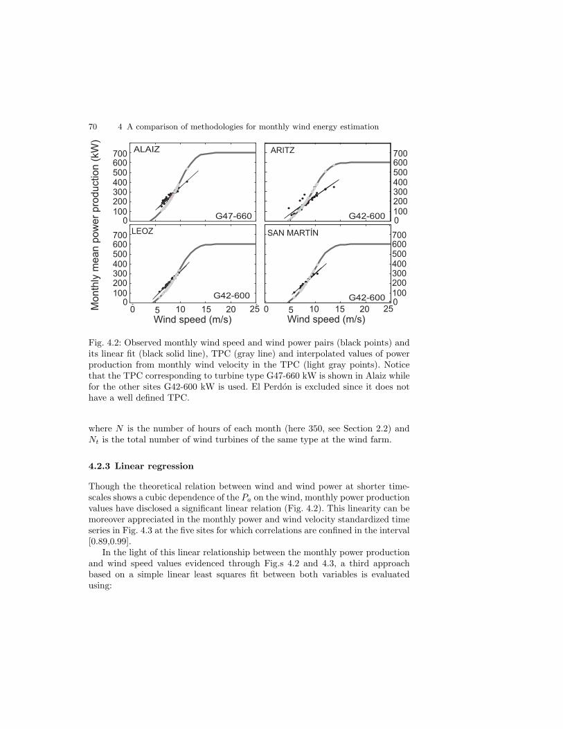
70 4 A comparison of methodologies for monthly wind energy estimation

Fig. 4.2: Observed monthly wind speed and wind power pairs (black points) andits linear fit (black solid line), TPC (gray line) and interpolated values of powerproduction from monthly wind velocity in the TPC (light gray points). Noticethat the TPC corresponding to turbine type G47-660 kW is shown in Alaiz whilefor the other sites G42-600 kW is used. El Perdon is excluded since it does nothave a well defined TPC.

where N is the number of hours of each month (here 350, see Section 2.2) andNt is the total number of wind turbines of the same type at the wind farm.

4.2.3 Linear regression

Though the theoretical relation between wind and wind power at shorter time-scales shows a cubic dependence of the Pa on the wind, monthly power productionvalues have disclosed a significant linear relation (Fig. 4.2). This linearity can bemoreover appreciated in the monthly power and wind velocity standardized timeseries in Fig. 4.3 at the five sites for which correlations are confined in the interval[0.89,0.99].

In the light of this linear relationship between the monthly power productionand wind speed values evidenced through Fig.s 4.2 and 4.3, a third approachbased on a simple linear least squares fit between both variables is evaluatedusing:

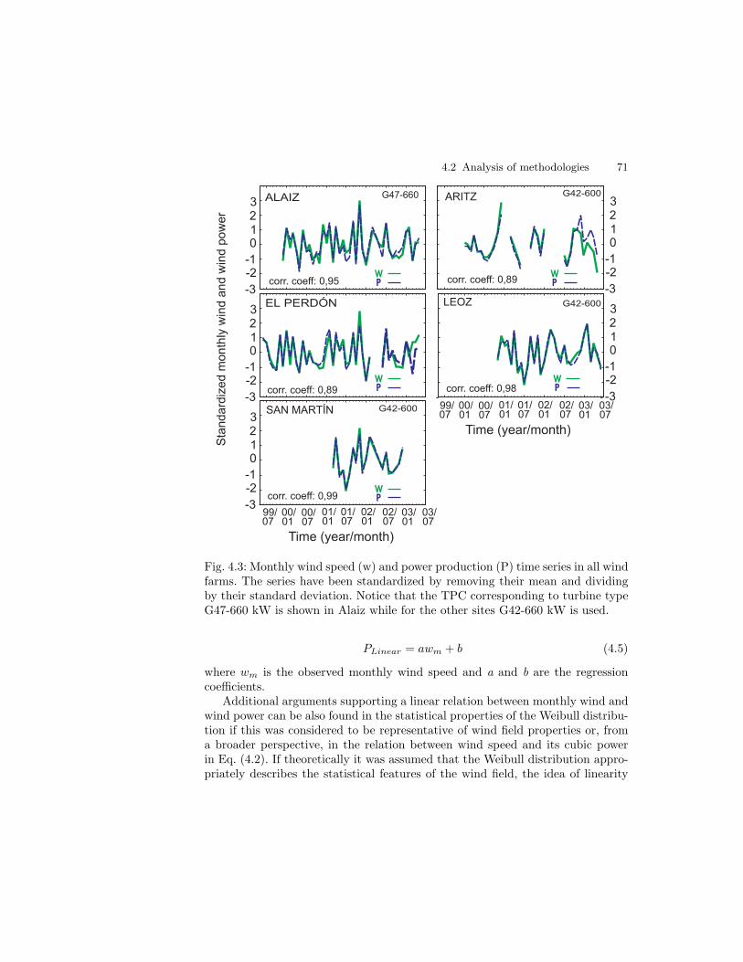
4.2 Analysis of methodologies 71

Fig. 4.3: Monthly wind speed (w) and power production (P) time series in all windfarms. The series have been standardized by removing their mean and dividingby their standard deviation. Notice that the TPC corresponding to turbine typeG47-660 kW is shown in Alaiz while for the other sites G42-660 kW is used.

PLinear = awm + b (4.5)

where wm is the observed monthly wind speed and a and b are the regressioncoefficients.

Additional arguments supporting a linear relation between monthly wind andwind power can be also found in the statistical properties of the Weibull distribu-tion if this was considered to be representative of wind field properties or, froma broader perspective, in the relation between wind speed and its cubic powerin Eq. (4.2). If theoretically it was assumed that the Weibull distribution appro-priately describes the statistical features of the wind field, the idea of linearity

72 4 A comparison of methodologies for monthly wind energy estimation

stems from the properties of this frequency distribution (Conradsen and Nielsen,1984), for which the n order moments are defined by:

E(wn) = cnΓ (1 +n

k) (4.6)

being w the wind speed, c the scale parameter and k the shape parameter. Then,the expected mean value, which would represent the monthly wind velocity, isdefined as E(w) = cΓ (1 + 1

k), and the third order moment, that would be repre-

sentative of the monthly wind energy carried by the wind if assuming a Weibulldistribution is E(w3) = c3Γ (1+ 3

k). The correlation coefficients for the calculated

monthly E(w) and E(w3) series range from 0.94 to 0.97 (not shown). Thus, agood approach to linearity between the wind speed and the energy carried bythe wind in the range of monthly values could be also considered if a Weibulldistribution was theoretically assumed.

Furthermore, the previous argument can be generalized for any frequencydistribution, by calculating the correlations between the monthly wind speed andthe available monthly power carried by the wind (Pa), represented by means of themonthly-averaged cubic wind speed. A dispersion diagram of the monthly windspeed and cubic wind speed is plotted in Fig. 4.4. The correlation coefficientsbetween both variables are 0.93 for Alaiz and Leoz, 0.94 for Aritz, 0.92 in ElPerdon and 0.95 for San Martın, respectively, thus supporting that linearity canbe a parsimonious assumption for the relation between wind speed and Pa forthe typical monthly range of values at the various sites.

The difference between Pa and the power generated by an ideal wind turbine(Pw) is that, in the case of Pw, the power production increases with the cubic windup to the rated wind speed (Chang et al., 2003). Finally, the differences betweenPw and the actual power generated are mainly due to the Cp(w) power coefficientin Eq. 4.2. This factor, at the range of values considered at monthly timescalesand for the turbine types described above, can be approached as constant (e.g.technical note, 1996). Thus, linearity can be a plausible assumption that is worthtesting also from this perspective.

In order to ensure independence in the building of the model in Eq. (4.5) asimilar process as in the case of the hourly based method (Eq. 4.1) was performed:each monthly PLinear estimation is obtained by inserting the corresponding wm

value into the linear regression previously calculated incorporating all the re-maining monthly wind speed-wind power pairs after excluding that of the targetmonth. This procedure was carried out consecutively for each month and sepa-rately for each one of the groups with similar wind turbines at farms with morethan one type of turbine. The total monthly wind energy estimation (wELinear)is computed as in Eq. (4.4), replacing PInterp with PLinear.

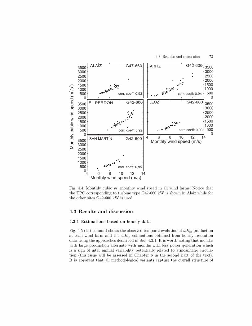
4.3 Results and discussion 73

S Lcorr. coeff: 0,93 S Lcorr. coeff: 0,94

S Lcorr. coeff: 0,92 S Lcorr. coeff: 0,93

S Lcorr. coeff: 0,95

Fig. 4.4: Monthly cubic vs. monthly wind speed in all wind farms. Notice thatthe TPC corresponding to turbine type G47-660 kW is shown in Alaiz while forthe other sites G42-600 kW is used.

4.3 Results and discussion

4.3.1 Estimations based on hourly data

Fig. 4.5 (left column) shows the observed temporal evolution of wEm productionat each wind farm and the wEm estimations obtained from hourly resolutiondata using the approaches described in Sec. 4.2.1. It is worth noting that monthswith large production alternate with months with less power generation whichis a sign of inter annual variability potentially related to atmospheric circula-tion (this issue will be assessed in Chapter 6 in the second part of the text).It is apparent that all methodological variants capture the overall structure of

74 4 A comparison of methodologies for monthly wind energy estimation

Fig. 4.5: Observed and estimated total monthly wEm time series (left col-umn) for all wind farms using hourly resolution data as described in Sec. 4.2.1.The optimal methodological estimations using the actual monthly EPC andhistogram, wEH−ref are compared to other variants, wEH−XXX (XXX ≡TPC,APC, PFC). wEH−APCw estimations including APC as an estimate ofEPC and a Weibull fit for the frequency terms are also shown. The correspond-ing estimation relative errors are represented in the right column.

4.3 Results and discussion 75

the temporal variability at all sites. The differences among the various energyestimations are smaller than the range of intra and inter annual variability. Thedifferent power production ranges at each wind farm seem to be also well rep-resented. The two methodological variants that produce the larger discrepanciesare the ones incorporating the TPC and the PFC (wEH−TPC , wEH−PFC). Thesimilarity between energy estimations and observations can be quantified withthe correlation (ρ) and the Brier skill score (β) statistics in Table 4.1 that mea-sure the concordance between observations and estimations and an estimate ofthe observational variance that the model accounts for, respectively (von Storchand Zwiers, 1999).

Table 4.1: Correlation (ρ)/Brier (β) skill score for the different methods.

ρ/β Alaiz Aritz El Perdon Leoz San Martın

wEH−ref 1.00/0.98 1.00/0.98 1.00/0.98 1.00/1.00 1.00/0.98wEH−TPC 0.96/0.87 0.90/0.71 -/- 0.99/0.68 0.99/0.83wEH−PFC 0.96/0.67 0.89/0.60 0.99/0.66 0.99/0.63 0.99/0.72wEH−APC 0.95/0.88 0.89/0.73 0.98/0.94 0.99/0.98 0.99/0.94wEH−APCw 0.92/0.76 0.84/0.72 0.96/0.85 0.94/0.59 0.96/0.91

wEInterp 0.94/0.56 0.81/0.52 -/- 0.97/0.82 0.98/0.83

wELinear 0.94/0.88 0.76/0.47 0.96/0.92 0.98/0.95 0.98/0.96

The wEH−ref estimations show the largest values of ρ and β (Table 4.1)indicating that, as expected, they reproduce best the variability in observations.The methodological variants incorporating the TPC, APC and PFC curves stilldeliver very high ρ and β values. The performance in terms of the β score is bestfor the wEH−APC estimations and worst for the wEH−PFC case. This suggeststhat assuming the TPC as a simple estimate of the relationship between windspeed and power production or the average of all available monthly power curves(APC) can produce as good performance or even better than more elaboratedpolynomial fits.

The additional use of Weibull estimates for the frequency terms further dete-riorates monthly energy estimations and provides a more realistic estimation ofthe error associated to this approach, due both to the f(wi) and pout(wi) terms.For simplicity reasons results in Fig. 4.5 and Table 4.1 are only shown for thecase of incorporating the APC power curve (wEH−APCw), which has producedthe best results so far. It is noticeable that in general the wEH−APCw estima-tion falls within the variability of the ensemble of methodological variants, thus

76 4 A comparison of methodologies for monthly wind energy estimation

suggesting that incorporating the error in the frequency terms is, in general, ofless relevance than changing the estimation used for the power terms. This com-paratively smaller impact does not necessarily point out a good quality Weibullfit as argued in Chapter 3.

Fig. 4.5 (right column) illustrates also the different performance of themethodological variants discussed above by showing the temporal evolution ofthe relative error: ξi = (wEobs−wEi)/wEobs. As indicated in Table 4.1 the small-est errors are produced by the reference methodological estimations, wEH−ref .The case of incorporating the APC power terms provides the second best estima-tions and the TPC and PFC cases tend to present negative (overestimation) andpositive biases (underestimation), respectively. This is due to the over- (under-)estimation of pout(wi) terms by the TPC (PFC) for large monthly wind speeds(see Fig. 4.1). In Fig. 4.5 this reveals a systematic behavior for which specific cor-rections could be developed at each wind farm, thus improving the performance ofthese model variants. Some methodologies can be found in the literature regard-ing potential improvements that could be used to derive more refined estimates ofthe power curve at each site than the ones used herein. For example, Pinson et al.(2007, 2008) applied nonparametric techniques providing probabilistic estimatesof the power production to evaluate the uncertainty associated with the windpower estimates and to derive a more accurate estimation of the power curve.Some other works use nonparametric statistical methodologies for different issuesrelated to the wind speed modeling, as for instance, in wind tunnel experiments(Hwang-Dae et al., 2007) or to correct bias, scattering or inhomogeneities in datacoming from a model (Caires and Sterl, 2005).

An overall perspective for the error at each site is provided in Table 4.2 wherethe average of relative and total errors is shown. For the calculation, absolutevalues at each time step have been considered to avoid cancellation of errors bychanges in sign. The worst estimations are obtained at Aritz for all methods. Theaverage error ranges between 0.9% and 5% for the five wind farms in the bestcase scenario for the hourly resolution method (wEH−ref ) and between 7.8%and 21.7% for the roughest power curve approximation case (wEH−TPC). Asdiscussed above, wEH−APC produces the best results of the three tested approx-imations with values ranging between 2.9% and 11.8%; these errors increase tovalues between 4.8% and 14.8% when the Weibull approximation is included. Asmentioned above, this comparatively small increase suggests that, in general, thecontribution to error of assumptions made in the power terms is more importantfor the sites studied herein than those concerning the fit to a theoretical proba-bility distribution. Yet, two amendments should be made to this statement. Thefirst one is that a clear exception takes place in Leoz where the average error in-creases from 2.9% to 10.0% after the introduction of the Weibull approximation.

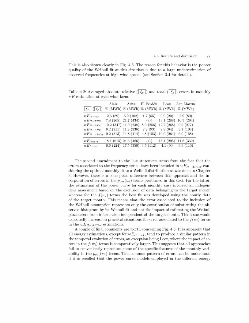
4.3 Results and discussion 77

This is also shown clearly in Fig. 4.5. The reason for this behavior is the poorerquality of the Weibull fit at this site that is due to a large underestimation ofobserved frequencies at high wind speeds (see Section 3.4 for details).

Table 4.2: Averaged absolute relative (| ξr |) and total (| ξt |) errors in monthlywE estimation at each wind farm.

Alaiz Aritz El Perdon Leoz San Martın

| ξr | (| ξt |) % (MWh) % (MWh) % (MWh) % (MWh) % (MWh)

wEH−ref 2.6 (89) 5.0 (102) 1.7 (55) 0.9 (20) 2.9 (80)wEH−TPC 7.8 (265) 21.7 (434) - (-) 13.1 (288) 10.5 (294)wEH−PFC 10.2 (347) 11.9 (238) 8.0 (256) 12.2 (268) 9.9 (277)wEH−APC 6.2 (211) 11.8 (236) 2.9 (93) 2.9 (64) 3.7 (104)wEH−APCw 9.2 (313) 14.8 (414) 4.8 (153) 10.0 (264) 6.0 (168)

wEInterp 18.1 (615) 24.3 (486) - (-) 13.4 (295) 11.8 (330)

wELinear 6.6 (224) 17.5 (350) 3.5 (112) 4.1 (90 3.9 (110)

The second amendment to the last statement stems from the fact that theerrors associated to the frequency terms have been included in wEH−APCw con-sidering the optimal monthly fit to a Weibull distribution as was done in Chapter3. However, there is a conceptual difference between this approach and the in-corporation of errors in the pout(wi) terms performed in this text. For the latter,the estimation of the power curve for each monthly case involved an indepen-dent assessment based on the exclusion of data belonging to the target monthwhereas for the f(wi) terms the best fit was developed using the hourly dataof the target month. This means that the error associated to the inclusion ofthe Weibull assumption represents only the contribution of substituting the ob-served histogram by its Weibull fit and not the impact of estimating the Weibullparameters from information independent of the target month. This issue wouldexpectedly increase in practical situations the error associated to the f(wi) termsin the wEH−APCw estimations.

A couple of final comments are worth concerning Fig. 4.5. It is apparent thatall energy estimations, except for wEH−ref , tend to produce a similar pattern inthe temporal evolution of errors, an exception being Leoz, where the impact of er-rors in the f(wi) terms is comparatively larger. This suggests that all approachesfail to conveniently reproduce some of the specific features of the monthly vari-ability in the pout(wi) terms. This common pattern of errors can be understoodif it is recalled that the power curve models employed in the different energy

78 4 A comparison of methodologies for monthly wind energy estimation

estimations do not consider the influence of several factors like the wind direc-tion or the air density, etc. The elaboration of a power curve that is valid forthe whole wind farm can involve many physical and engineering aspects to betaken into account in order to represent in detail the global wind speed-windpower relation (Noorgard and Holttinen, 2004). Previous work has attempted toillustrate for instance the uncertainty in the energy production estimation thatarises from the use of a specific wind turbine power curve (Lange, 2005; Lackneret al., 2008). Also, Pinson et al. (2008) employ an advanced nonparametric sta-tistical approach to adequately estimate the conversion function from wind speedto wind power. Such a refinement of the energy estimations or the inclusion ofspecific corrections for each power curve model is out of the scope of this workand from such perspective the power curve models used herein are parsimoniousand all omit a number of complexities that can lead to the common pattern oferrors in Fig. 4.5.

It is also interesting to highlight the increase of error produced by all method-ological variants, including wEH−ref , in Aritz at the end of the observational pe-riod. The causes for this overall failure that produces the largest errors have notbeen elucidated. This behavior suggests problems with the quality of data as aplausible cause that would deteriorate the performance of the reference estimatewEH−ref and consequently also of the others.

4.3.2 Estimations with monthly data and comparison with the hourlycase

Fig. 4.6 allows for extending the assessment to the performance of the two verysimple approaches described in Sections. 4.2.2 and 4.2.3 (wEInterp and wELinear).Results for ρ and β as well as for relative error averages are also shown in Tables4.1 and 4.2. For clarity purposes only the wEH−APCw variant, which involvesthe more realistic assessment of errors in Fig. 4.5, is included in Fig. 4.6 forcomparison.

It can be appreciated in Fig. 4.6 (left column) that both wEInterp andwELinear reveal quite a good performance in comparison to wEH−APCw in spiteof the rough approximations adopted. The wEH−APCw and wELinear estimationsare very similar in all cases and they are additionally very close to the observedvalues. This is also evidenced in Fig. 4.6 by the relative errors of the differentestimations (wEH−APCw, wEInterp and wELinear) and in the statistics in Tables4.1 and 4.2. The interpolation method, although is able to replicate their tem-poral structure and reasonably captures the variability of observed time seriesin the wind farms (the explained variance is 89%, 66%, 95% and 96% for Alaiz,Aritz, Leoz and San Martın, respectively), presents the largest errors, as shownin Fig. 4.6 (right column), in the higher error averages of Table 4.2 and in the

4.3 Results and discussion 79

Fig. 4.6: Left: observed and estimated total monthly wE (wEH−APCw, wEInterp

and wELinear) time series for all wind farms. Right: corresponding relative errors.

80 4 A comparison of methodologies for monthly wind energy estimation

decrease of the Brier score values in Table 4.1. This is due to an overestimationof variability by this method produced by the larger tilt of the TPC relative tothe observed wind speed-wind power relationship at monthly timescales (see Fig.4.2). It can be argued that the TPC is calculated to represent the relationshipbetween wind speed and wind power for 10-minute resolution data. Its use asan estimation of the EPC in wEH−TPC in an hourly resolution data approach isadmissible in view of the results shown in Fig. 4.5 and Tables 4.1 and 4.2. The useof monthly averages involves changes in the relationship between wind speed andwind power (Fig. 4.2) that are not well captured by an interpolation in the TPC.The reason is the use of the averaging operator (which is linear) over a curvethat is essentially not linear, except at intermediate range of wind values whereit can be approached as a quasi-linear curve (see discussion in section 4.2.2).Nevertheless, wEInterp still captures the temporal variability in the observations(Fig. 4.6) and thus, it may prove useful when monthly wind energy estimationsare required in situations of no availability of power production observations (seeChapter 6).

The more interesting feature in Fig. 4.6 is perhaps the fact that wEH−APCw

and wELinear produce a similar performance. wELinear performs worse in Aritz(see Tables 4.1 and 4.2) and compares well or outperforms wEH−APCw in therest of the sites. In Leoz, where the impact of the frequency terms produces largerdeviations in wEH−APCw, wELinear does visibly better (Fig. 4.6, right column).In addition, in practical situations the error associated to wEH−APCw could beexpected to increase if we recall the fact that these estimations incorporate onlya lower limit estimation of the error in the frequency terms (see independencearguments raised above). This argument further endorses the performance of aparsimonious simple linear regression in comparison with more elaborated ap-proaches. Therefore, not only does the linear approach achieve comparably goodresults, but also it constitutes a simple and robust methodology operating onmonthly resolution data.

It is also interesting to notice that the temporal evolution of errors in Fig. 4.6,in particular those of wEH−APCw and wELinear, is correlated (values not shown).Such changes in wELinear can only stem from deficiencies in the representationof the monthly variability of the slope in the linear regression. Therefore, thissupports the idea that in the case of wEH−APCw and the methodological variantsincluded in Fig. 4.1 the common temporal structure of error derives from commondeficiencies in the representation of the tilt of the power curve.

4.4 Conclusions 81

4.4 Conclusions

In this work three methods have been compared in their performance to esti-mate monthly wind energy. The first strategy makes use of hourly resolutiondata and builds estimates based on the wind speed frequency distribution and ona transfer function that expresses the relationship between wind speed and windpower at these time scales. Different estimates have been analyzed: the observedmonthly power curves (EPCs), the theoretical power curve provided by manu-facturers (TPCs), the average of the available EPCs (APCs), or a polynomialfit to them (PFCs). Observed frequency histograms have also been replaced byWeibull estimations to take into account the influence of the frequency terms.The selection of these power and frequency estimates has been done on the basisof their simplicity and/or standard use.

In the second approach, the TPC has been used to obtain monthly values ofpower production through an interpolation procedure using directly the monthlywind velocity. Some evidences of the linear relationship existing between windand power production at monthly timescales are shown, in spite of the expectedcubic relation between both variables. Thus, the last approach considered hereconsists in a simple linear regression calculated over the monthly wind speed-windpower pairs.

All methods and methodological variants used pick up the intra and interannual variability of energy production at all wind farms. The hourly approachproduces minimal errors when the EPC and monthly frequency histograms areused in wEH−ref and they are raised most often below 20% (below 15% onaverage) when power curve and frequency approximations are used. The APCprovides a simple and straight forward estimation for the power terms that leadsto the best results.

The inclusion of the Weibull approximation raises the error, particularly atsites where the quality of the fit is clearly bad as in the case of Leoz. The resultsachieved in this work suggest that the choice of a power curve is more criticalthan the errors stemming from using a Weibull fit to the data.

The interpolation based method provides wEInterp estimations that tend tooverestimate monthly wind energy variability due to a larger tilt in the TPC thanin the observed relationship between wind speed and wind power at monthlytimescales. Nevertheless, monthly energy estimations with this approach may beuseful in situations of unavailability of power production data.

The hourly based and linear regression methods perform comparably in spiteof the simplicity of the linear regression approach. This supports the use of re-gression estimates in estimations of energy production from monthly resolutiondata.

82 4 A comparison of methodologies for monthly wind energy estimation

Estimating the wE production from the wind at monthly timescales basedon the robust knowledge of the wind speed-wind power relationship can be use-ful in the medium and long term framework. For instance in an empirical ordynamical downscaling context where the wind speed is derived through its rela-tion with the large scale circulation and afterwards the wind energy is estimatedfrom the wind velocity. Some previous works that assess the past variability ofthe wind and wind energy density and evaluate possible changes in the windenergy resources in potential climate change scenarios can be found in the lit-erature (Pryor et al., 2005b; Pryor and Schoof, 2005; Kaas et al., 1996; Pryoret al., 2005a, 2006). The empiric linearity between the two variables at monthlytimescales involves an additional interesting alternative: the direct estimation ofthe wind energy production from its relation with the synoptic atmospheric flow.It can be expected that such a relation presents similar properties as the relationbetween the wind and the atmospheric circulation at monthly timescales due tothe empirical linearity observed between wind velocity and power production atthese timescales. These issues are explored in the second part of this work wherethe regional wind variability will investigated in terms of its relationship with thelarge scale atmospheric circulation and the wind power production will be con-sidered as an impact variable providing a framework to examine its predictabilityin the basis of changes in the large scale circulation.

Part II

Wind and wind power dependence on

large scale atmospheric circulation

5

North Atlantic atmospheric circulation and

surface wind in the Northeast of the Iberian

Peninsula∗

¿Sabe el mar como se llama, que es el mar? ¿Saben los vientos sus apellidos,

del Sur y del Norte, por encima del puro soplo que son?.

Pedro Salinas. La voz a ti debida, 1933.

In the first part of this thesis the relationship between wind speed and windpower production was explored. The wind measured at various wind farms inthe CFN has been analyzed on the basis of the implications that assuming acertain PDF has on the production of wind energy. A suite of methodologiesfor the estimation of wind power were investigated leading to disclose a relationbetween both variables that can be assumed as linear at monthly timescales.This last conclusion will show relevant consequences in the analysis of the windpower variability as a meteorologically-driven variable. In this second part of thework a different perspective is adopted in which both, wind and wind powerare analysed through their relation with the large scale atmospheric circulation.Thus, transfer functions translating the large scale information to the regionalscale will be derived by applying statistical downscaling techniques.

In this chapter the variability and predictability of the surface wind fieldat the regional scale over the CFN is explored. A downscaling technique basedon Canonical Correlation Analysis (CCA) allows for calibrating and validatinga statistical method that elicits the main associations between the large scaleatmospheric circulation over the North Atlantic and Mediterranean areas andthe regional wind field. In an initial step the downscaling model is designed by

∗ The main contents of this chapter are included in:Garcıa-Bustamante, E., J. F. Gonzalez-Rouco, J. Navarro, E. Xoplaki, P. A. Jimenezand J. P. Montavez, 2011: North Atlantic atmospheric circulation and surface windin the Northeast of the Iberian Peninsula: uncertainty and long term downscaledvariability. Clim. Dyn.. DOI 10.1007/s00382-010-0969-x.

86 5 North Atlantic circulation and local wind

selecting parameter values from practise. To a large extent, the variability of thewind at monthly timescales is found to be governed by the large scale circulationmodulated by the particular orographic features of the area. The sensitivity ofthe downscaling methodology to the selection of the model parameter values isexplored, in a second step, by performing a systematic sampling of the parameterspace. The downscaling model is used to extend the estimations several centuriesto the past using long datasets of sea level pressure, thereby illustrating the largetemporal variability of the regional wind field from inter annual to multicentennialtimescales. The analysis will not evidence large long term trends throughout thetwentieth century, however anomalous episodes of high/low wind speeds will beidentified.

In Section 5.2 the main aspects of the methodology applied are reviewed. Sec-tion 5.3 illustrates the results of calibrating and validating the statistical tech-nique applied, showing the pairs of optimally correlated patterns for the synopticand the local scales, respectively, and the estimations obtained after the methodis validated against the available observations. The results within this section willbe referred to as the reference case, where a certain configuration of the modelis selected with illustrative purposes. Section 5 highlights the assessment andimplications of the associated uncertainty combining the large scale influence inthe estimations with various methodological aspects that could introduce somevariance in the results obtained. In Section 6 the long term variability of thewind field over northern Iberia is evaluated in the base of a reconstruction of thewind climatology for approximately the past three centuries. Finally, Section 7presents and discusses the main conclusions.

5.1 The regional climate problem: the role of the

downscaling techniques

The improved understanding of the regional/local wind variability and its relationto the large scale atmospheric circulation, greatly benefits applications targetingthe prediction of wind related variables. Assessments of climate variability atthe regional scale are mainly based on the application of dynamical or statisticaldownscaling approaches that attempt to bridge the gap between the informationprovided by large scale datasets as GCMs outputs, reanalysis, etc. and the reliableestimations required at the regional scale by increasing the spatial resolution.

A broad classification of the downscaling techniques divides them into dynam-ical or statistical (Chapter 1). The dynamical approach involves the use of a RCMthat, feeded by large scale boundary conditions, solve the fundamental equationsof the atmosphere yielding estimates at refined resolutions. Thus, RCMs are ableto provide a coherent response with the large scale boundary conditions and the

5.1 The regional climate problem: the role of the downscaling techniques 87

physics involved in the cascade of multiple processes to achieve local resolutions.Boundary conditions are usually provided by large scale reanalysis (Hong andKalnay, 2000; Herrmann and Somot, 2008; Conil and Hall, 2006) or by the out-puts of a GCM (Pryor et al., 2005b; Lenderink et al., 2007). Some examples inthe context of wind field analysis can be cited: Pryor et al. (2005a) studied theimplications of the long term wind variability for the wind energy resources overnorthern Europe using RCMs; Winterfeldt and Weisse (2009) explored the abil-ity of two RCMs to reproduce instantaneous values and frequency distributionof surface marine winds over the North Atlantic highlighting the added value ofRCM simulations compared to reanalysis data and Jimenez et al. (2010b) eval-uated the ability of a RCM to identify subregions with similar wind behaviourthat was previously found with observations over the same area in the northeastof the Iberian Peninsula (IP).

In turn, the statistical downscaling consists in training a statistical modelmaking use of the empirical relationships observed between the local variables,predictands and the large scale atmospheric variables, predictors (Gonzalez-Roucoet al., 2000; Xoplaki et al., 2004; Busuioc et al., 2008). The classification of statis-tical methods entails a certain degree of subjectivity. In broad terms they can besegregated in analog methods (Zorita and von Storch, 1999), classification tech-niques (Yarnal, 1993), linear models (Xoplaki et al., 2004) and more sophisticatednon-linear approaches, as the neural networks (Hewitson and Crane, 1996), andtheir use depends on the particularities of the problem. Linear methods, for in-stance, are widespread used within the context of empirical techniques and thespecific method may involve different levels of complexity.

Statistical tools have been widely employed with large scale sea SLP or seasurface temperature (SST) observations to understand the regional precipitationand temperature variations (Zorita et al., 1992; Zorita and von Storch, 1999;Xoplaki et al., 2003a,b, 2004). However such methodologies have not been ex-tensively applied to wind related variables. Some examples can be cited: Kaaset al. (1996) identified the connection between SLP/SST patterns and the localwind field in winter over Scandinavia; Faucher et al. (1999) provided an empiricalreconstruction of surface winds using observations from buoys along the westerncoast of Canada; Pryor and Schoof (2005) proposed an empirical downscaling toestimate variations in the parameters of a typical wind probability distributionat the regional scale in northern Europe; Klink (2007) investigated the relationbetween the large scale atmospheric circulation and the wind at typical windturbine heights in central United States (US) using a regression approach andDavy et al. (2010) applied a novel approach based on machine learning strate-gies combined with a linear regression and a classification scheme to explore thelarge scale influence on the wind field variability over south-eastern Australia. An

88 5 North Atlantic circulation and local wind

extended application of these methods consists in forcing the statistical modelwith the conditions in a climate change scenario simulated by a GCM (Denmanet al., 2007). Some examples concerning statistical approaches for future climateprojections deserve attention: Bogardi and Matyasovszky (1996) combined a cir-culation classification scheme with multivariate regression to interrelate localwind and large scale atmospheric patterns and studied the impact of a doublingCO2 scenario in Nebraska; Sailor et al. (2000, 2008) employed neural networks toassess the effects of some climate change scenarios on wind power resources andgeneration over northwestern US; Najac et al. (2009) applied a statistical down-scaling to a multi GCMs ensemble and estimated future changes of the wind fieldover France in a particular future climate scenario. In this chapter the variabil-ity and predictability of the wind field over the CFN is investigated through astatistical downscaling model based on CCA that searches for the associationsof large scale predictors in the North Atlantic and Mediterranean areas and thelocal wind.

Downscaled estimations allow for an understanding of climate variability atthe regional scale, but they are also subject to uncertainties that are seldomconsidered. Uncertainty can be propagated from the global to the regional scaleand will be additionally increased in the downscaling step (Mitchell and Hulme,1999; Schwierz et al., 2006). At the global and large scales, uncertainty per-meates through the use of different versions of instrumental datasets reanalysisproducts or GCMs when, for instance downscaling models are calibrated. All ofthem produce similar but non-identical representations of climate and will addvariability to the downscaled estimations. If experiments in the context of futureclimate change scenarios are considered, the use of different forcings scenariosand different GCMs will further contribute to this. The use of downscaling mod-els adds to the pool of uncertainty from three main sources. One of them is thespecific downscaling scheme selected for the experiment from a variety of dynam-ical or statistical downscaling approaches (hybrid cases also included) that willproduce purportedly similar albeit non-identical results. Once the methodologyis selected, there is often a multiplicity of available parameter and configurationoptions that are based on experience and that also have an impact on the results.Finally, although at the top of the hierarchy of importance, we are subject to ourrepresentation of reality by the regional/local observational datasets, that playthe role of validation benchmarks for dynamical downscaling or calibration andvalidation data in the case of statistical downscaling. A proper representation ofthe cascade of uncertainties would imply a sampling of all possibilities of changeat each step of this hierarchy. This would picture the range of all possible estima-tions attained with the available methods and datasets. This type of assessmentcan be regarded as a frequentist approach (see Chapter 1)

5.2 Downscaling methodology 89

If we consider the downscaling step, the evaluation of methodological uncer-tainties stemming from the use of different model configurations is not extensivelyexplored within the statistical downscaling approaches. Here, the uncertainty as-sessment is based on the examination of the effects that variations of the modelparameters can have. These parameters involved in the model configuration thatare investigated in this step are for instance the size of the geographical domainof the large scale predictors or the number of canonical patterns retained for theanalysis. The uncertainty that arises from the use of different datasets as largescale predictors (reanalysis data, observations or climate field reconstructions)is also evaluated. The combination of both sources of uncertainty will provide amore reliable estimation of the wind field variability. An additional benefit of ob-taining a measure of the uncertainties that arise in the downscaling step impliesthat in subsequent stages of the work they could be compared to those derivedfrom the use of different GCMs in future climate change projections or thosecoming from the use of different scenarios. In such conditions a representation ofthe full cascade of uncertainties involved in future regional climate projectionswould be feasible.

The understanding of the mechanisms responsible for the temporal variationsof the regional wind at inter decadal and centennial timescales is hampered bythe limited temporal length of the observational series since usually short periodsare used for calibrating and validating models. The statistical methodology ap-plied allows for extending the wind estimations several centuries backward in theabsence of wind observations using the available datasets of large scale predictorvariables. The long term variability of the regional wind is interpreted in terms ofthe variations in sign and intensity of the main modes of the atmospheric circu-lation affecting the regional wind that were found during the calibration period.This exercise provides a broader perspective of the regional wind variability inobservations that may be of use in the context of comparison with climate changedownscaling exercises. To the knowledge of the authors, this approach has notbeen documented in the literature before.

5.2 Downscaling methodology

The statistical method applied in this study is based on CCA. This is a multi-variate statistical technique that isolates linear associations between sets of pre-dictor and predictand variables that are optimally correlated (Hotelling, 1935,1936; Glahn, 1968; Levine, 1977). The original data are projected onto theirprincipal components (PCs) to remove noise and reduce the number of degreesof freedom. This method was first proposed by Pearson (1902) and applied firstto the meteorology context by Lorentz (1955). The CCA selects pairs of spatial

90 5 North Atlantic circulation and local wind

patterns from a set of several space-time dependent fields that have maximumcorrelation coefficient and generates new pairs of variables from the original fieldsby linear combination of them. They are called canonical component vector orcanonical coordinates, present maximum correlation and they are normalised tounit variance. The original variables can be expressed as a linear combinationof its canonical coordinates and its canonical correlation patterns. The last arethe result of projecting the original fields onto the canonical component vectorsspace. The canonical coordinates or scores represent the intensity of the modesfound, that is, they describe the amplitude and sign of the corresponding pat-terns at each time t. To obtain an estimation of the field of interest, a regressionmodel is designed. It represents the predictand variable as a linear combinationof the canonical coordinates and the patterns obtained during the analysis. Themethodology is further described in von Storch and Zwiers (1999).

Before calibrating the model, the annual cycle is removed by subtracting themonthly climatological mean to obtain anomaly fields. Time series were alsodetrended applying a linear least square fit in order to ensure the long-termstationarity (Xoplaki et al., 2003b). In order to account for the latitudinal distor-tions, anomalies from the large scale fields were weighted at each grid point bymultiplying by the square root of the latitude to consider the decreasing size ofgrid boxes with latitude (North et al., 1982b). Additionally the time series werestandardized (dividing by their standard deviation). The size of the matrices al-lowed for managing the problem in a single step. Eventually, the same number ofmodes from both predictor EOFs were retained, as they accounted for a similaramount of explained variance, for the posterior combined CCA (Preisendorfer,1988; von Storch and Zwiers, 1999).

A certain combination of the model parameters was selected in a first stepof the analysis. This selection does not correspond to the optimal case, althoughit generates reasonable estimates of the wind field. This selection, prior to thesensitivity analysis, represents a standard situation (thereafter called referencecase) to illustrate the potential of the methodology and allows for understandingthe emergent associations between predictors and predictands. The choice of pa-rameters for this reference case is exposed in Section 5.3.1. However, variations inthis selection and their influence on the results will be explored in the sensitivityanalysis in Section 5.4.

After the design of the downscaling model, its skill is verified using a crossvali-dation approach. This allows to reduce a possible overfitting of data by the model(Barnett and Preisendorfer, 1987). The crossvalidation is a resamplig techniquein which a small number of data is dismissed and the model is trained with theretained data subset. The removed values are then estimated with the calibratedmodel. This procedure is repeated recursively by sampling subsets of the same

5.3 Wind estimations in the CFN: the reference case 91

length along the entire observational record in order to obtain a full set of in-dependent estimates that are compared afterwards to the original observations(Michaelsen, 1987). Further details on the size of the sampling subsets are givenin the following sections.

The actual extended winter season dataset analysed herein is composed of 91monthly wind observations at each site (14 yrs x 7 months/year) and thus hardlyspans more than a decade. It can be argued this is a limitation for the analysisand should not be forgotten in the interpretation of results since the model is cali-brated making use of intraseasonal to decadal crosscovariances and it is assumedto reproduce wind variability at multidecadal and even centennial timescales.This assumption is however not alien to downscaling approaches where the bestuse of available data has led in some analysis to calibrate models based on com-paratively short decadal records (Huth, 2002, 2004; Orlowsky et al., 2008) or, ina more typical approach, to use multidecadal long records to estimate variabilityon centennial and longer timescales (e.g., Gonzalez-Rouco et al., 2000; Xoplakiet al., 2003a). On the other hand, the afore mentioned crossvalidation approachcontributes to ensure the robustness of the statistical relationships and reducespossible overfitting of data (Barnett and Preisendorfer, 1987).

To evaluate the predicting skill of the method, the correlation coefficient (ρ)and the Brier Skill Score (β) have been used in this work. ρ yields a measure ofthe temporal concordance between the observations and estimations. β providesa measure of the variance of observations that is accounted for by the model. Thiscoefficient is defined as β = 1 −

[

S2ES/S2

OB

]

, were S2ES represents the variance

of the estimations error and S2OB is the observations variance, provided that the

climatology is selected as reference value to evaluate the error. In such conditionsβ = 0 represents a prediction not better than climatology. If the estimations errorvariance is similar to that of the observations a positive β is obtained (the betterthe prediction, the closer to 1).

5.3 Wind estimations in the CFN: the reference case

In this section results from the calibration of the statistical downscaling model arepresented (Section 5.3.1) and evaluated (Section 5.3.2). This will serve as a ref-erence configuration hereafter. Monthly zonal (west-east) and meridional (north-south) components of the wind are employed as predictand fields. These windfield observations were presented in Section 2.3. Additionally, for this exercise,wind data from three wind farms are included to illustrate potential differencesin the influence of the large scale circulation on the local wind since in the windfarms data is recorded at heights between 30-40 m and typically on the top of themountains or hills (recall Section 2.2). Using wind components instead of wind

92 5 North Atlantic circulation and local wind

module introduces directional information that helps to interpret the influenceof the large scale circulation and the orography on regional flows. This allows fortaking into account the direction of the flow in the search of relations betweenthe regional wind and the large scale circulation since it implies a segregationof large scale circulation patterns that would be merged if the wind module isemployed as predictand.

In the reference case two ERA-40 fields (see Section 2.4), φ850 and Z500−850,are used as predictors as they provide a dynamical and thermal description of theatmospheric circulation. The analysis is limited to a geographical area spanningfrom 35oN to 65oN and 40oW to 10oE, which includes the western North At-lantic area, the Iberian Peninsula, the British Isles, the westernmost region of theEuropean continent and part of the Mediterranean basin. This spatial windowhas been used in studies addressing the connections between circulation patternsover a similar Atlantic area and local variables in the IP and Mediterranean ar-eas: temperature (e.g., Xoplaki et al., 2003a,b), precipitation (e.g., Trigo et al.,2004) and solar radiation (e.g., Pozo-Vazquez et al., 2004). 4 predictor EOFs areretained for the analysis, accounting for a 81.5% of the total variance. The samenumber of EOFs is considered for the predictand that account for a 90.2% of thevariance. 2 pairs of canonical modes are retained in the design of the downscalingmodel. In the reference configuration the size of the crossvalidation sampling sub-set is one month. This selection does not necessarily correspond to the optimalcase. The choice of model parameters is based on a prior heuristic explorationof several model configurations, as a previous step to the sensitivity analysis,to gain some insight about the variance within estimates due to changes in themodel parameters. Thus, this configuration was selected for illustration purposesand provides estimations in good agreement with observations. In section 5.4variations of this reference configuration will be explored.

5.3.1 Canonical patterns and series

The first pair of canonical patterns (CCA1) is represented in Figs. 5.1a,b for thepredictor and predictand variables, respectively, together with their amplitudetime series or canonical coordinates (Fig. 5.1c). The large scale pattern (Fig.5.1a, shaded for φ850 and contours for Z500−850) depicts a dipole structure withpositive anomalies over the North Atlantic area, that reaches the west side of theIP. Negative anomalies are located northeast of the British Isles, centred over theScandinavian Peninsula. The simultaneous CCA1 pattern for the predictand (re-gional wind) presents in its positive phase NW-SE wind oriented anomalies whichcan be related to the well known regional ’Cierzo’. It should be noticed that thereverse sign of the patterns is also possible since it is determined by the sign of

5.3 Wind estimations in the CFN: the reference case 93

eigenvalues of the cross-covariance matrix (von Storch and Zwiers, 1999). There-fore, the negative phase of this mode presents contributions to the flow fromthe SE with relatively warm and moist air advection from the Mediterraneanthat can be regarded as the typical ’Bochorno’. The two patterns are physicallymeaningful provided that the large scale mode induces a pressure gradient thatfavours a NW-SE (SE-NW) direction for the geostrophic wind. In addition, theaxis of the Ebro Valley, aligned with this NW-SE direction, contributes with astrong channeling effect at the surface. Thus, the local wind pattern arises asa result of the large scale atmospheric structure modulated by the orographicconfiguration of the CFN. This first mode accounts for 18% (22%) of the totalvariance of the φ850 (Z500−850) predictor field and around 36% of the total pre-dictand variance (see Table 5.1 for summarized information on correlations andexplained variances). It is interesting to mention that, in agreement with a moremeridional large scale circulation, in this canonical mode the largest amount ofexplained variance (46%) corresponds to the meridional component of the windwhile in the case of the the zonal one, the CCA1 accounts for a smaller portion(25%) of variance. The same large scale regime as found here, that causes a par-tial blocking of the westerlies, has been associated with the Mistral conditions(Buzzi et al., 2003; Burlando, 2009). Thus, this large scale pattern is broadlyresponsible for predominant meridional circulations not only in the region understudy, but also in wider areas over the European continent.

Table 5.1: Canonical correlations and explained variances by the CCA modes.

Corr. φ850/Z500−850 expl. var.(%) Predictand expl. var. (%)

CCA1 0.87 18/22 36CCA2 0.86 30/13 36

The corresponding amplitude series for predictor and predictand (Fig. 5.1c)present a canonical correlation of 0.87 and exhibit considerable intra and interannual variability with extreme values at the end of 1995 and 1999. The variabilityis higher till 2000 and slightly lower in the following period. As this change in theregional wind variance during the last period is also noticeable in the predictorseries, it can be attributed to changes in the large scale circulation variability. Thecanonical series of the local wind components presents a correlation of 0.92 and-0.83 with the regional time series of the observed zonal and meridional windcomponents (Fig. 2.6), respectively. Thus, this first canonical mode describes

94 5 North Atlantic circulation and local wind

Norm

aliz

ed t

ime c

om

ponents

Time (year)

1992 1994 1996 1998 2000 2002 2004 2006

4

3

2

1

0

-1

-2

-3

-4

Fig. 5.1: Canonical patterns and series of the first CCA mode (CCA1). a) Pre-dictor patterns, φ850 hPa (shaded) and Z500−850 hPa (contours); the explainedvariance of the φ850 (Z500−850) field is also indicated; b) predictand (local windin the CFN) pattern together with the variance accounted for by this mode; windfarms are represented with white squares. c) canonical series for predictor (blue)and predictand (green).

5.3 Wind estimations in the CFN: the reference case 95

the most important changes in regional monthly wind variability for the periodstudied.

The second pair of coupled patterns (CCA2) shares 30% (13%) of varianceof the φ850 (Z500−850) field and 36% with the regional wind or predictand. Notethat this second mode accounts for larger amount of variance of the zonal compo-nent (40%) than in the case of the meridional one (33%) which is consistent witha more zonal large scale forcing. In fact, the canonical predictor mode consistsof a monopole pattern of negative anomalies centred westward of the BritishIsles. This pattern in its positive phase indicates a zonally eastward orientedgeostrophic flow. The CCA2 wind pattern (Fig. 5.2b) shows a configuration witha more zonal direction at most of the windiest sites over the northern and centralpart of the region, that coincide with the wind farm locations. These sites aremore exposed to quasi-geostrophic circulations and less affected by local scalephenomena. For the rest of stations, the surface wind field displays a SE-NWdirection which is coherent with a deflection of the geostrophic wind that tendsto balance the horizontal pressure gradient and helps to introduce southern sur-face flows in the valley mouth. Hence, this mode in its positive (negative) phaseevidences contributions to the Bochorno (Cierzo). This coupled mode shows adecisive impact of the orography, contributing for instance to circulations thatare prone to be channeled along the Ebro valley due to the strong orographicconstraint. It additionally evidences an important influence of the large scalecirculation since some stations in central and northern CFN or the wind farmlocations, which are not subject to the channeling effect at the valley, show amore zonal response to that mode. The correlation between the CCA2 time com-ponents is 0.86 (see Table 5.1). They show large intensity contributions in 1993and during the period between 2000 and 2002 and also reveal a considerable intraand interannual variability.

It is well worth to discuss the relation of the canonical large scale modes withthe main teleconnection patterns in the Atlantic area. The Iberian Peninsulaand especially the CFN, is geographically located at the boundaries of the stormtrack in the North Atlantic region and potential fluctuations of the differentmodes over the climate of the region can be expected (Seierstad et al., 2007).The low frequency patterns affecting the European continent are (Barnston andLivezey, 1987): the North Atlantic Oscillation (NAO), this being the preferredmode in this area affecting all seasons and influencing the intensity of zonaland meridional heat and moisture transport; the East Atlantic Pattern (EA),a second predominant mode considered as a southward shift of the NAO andalso linked with subtropical low frequency variability; the East Atlantic/WesternRussia pattern (EA/WR) -a four-center pattern affecting Eurasia during the

96 5 North Atlantic circulation and local wind

Time (year)

1992 1994 1996 1998 2000 2002 2004 2006Norm

aliz

ed t

ime c

om

ponents 4

3

2

1

0

-1

-2

-3

-4

Fig. 5.2: As in Fig. 5.1 but for the second CCA mode (CCA2).

whole year and finally the Scandinavian (SCAN) pattern, which has somewhatweaker centers of opposite sign located over western Europe and western Russia.

In Table 5.2, the correlations between the first two canonical series of thepredictor fields and the indexes of the teleconnection patterns are given (Barnstonand Livezey, 1987)†. Most of the correlation values are significant at a 0.05 level(in bold). However, the highest correlation with the CCA1 large scale canonicalseries is found with the East Atlantic/Western Russia mode (EA/WR; Burlando,2009). In the case of the CCA2, the strongest relation is found for the EastAtlantic pattern (EA).

† www.cpc.ncep.noaa.gov/data/teledoc/telecontents.shtml

5.3 Wind estimations in the CFN: the reference case 97

Table 5.2: Correlation values between the two first canonical series and the mainlow frequency teleconnection patterns over the Atlantic area: NAO, EA, EA/WRand SCAN.

NAO EA EA/WR SCAN

CCA1 0.16 0.28 -0.47 -0.32

CCA2 -0.24 0.46 0.20 0.27

5.3.2 Validation of wind estimates

The estimated regional anomalies for the zonal and meridional wind componentsand wind module are compared to their observational counterparts in Fig. 5.3.The correlations between the regional estimations and observations are 0.79 and0.80 for the zonal and meridional component, respectively and 0.70 for the windmodule (all correlations are significant at a 0.05 level). The lower correlation ofthe wind module can be understood on the basis of the non-linear transforma-tions applied to obtain it from the wind components together with the potentialaccumulation of the errors from each component. The higher variability of themeridional component becomes evident again. It can be observed that the esti-mations show also reduced variance with regard to the observations. This loss ofvariance is inherent to the linear methodologies (von Storch and Zwiers, 1999).

The skill of the method at each station is evaluated through the values of ρand β represented in Figs. 5.4a,b,c. This inspection allows for a validation of theprocedure at the local scale providing an overview of the predictability dependingon the specific location. The size of circles is proportional to the correlation (ρ)value and the color is related to the Brier skill score (β). At most locations thecorrelation values range from 0.85 to 0.50 for both wind components. Also theBrier skill score shows a reasonably good performance of the model in terms ofthe variance error (values span the interval 0.72 to 0.30). A few locations at thenorthern areas and some stations at the mainland valleys show a decay of theskill in both their ρ and β values. These stations are located in less windy sites(Fig. 2.5) or in areas with more complex orography that contributes to a decreaseof the predictability. Overall, the pattern is very similar for both components buthigher scores can be observed along the NW-SE axis of the Ebro Valley for themeridional one. The main differences between them are found in the northernand the mountain stations, where the zonal component predictability is slightlydeteriorated. The wind module as in the case of the regionally averaged seriesshows also slightly worse performance compared to the two wind components.

98 5 North Atlantic circulation and local wind

corr. 0.79

corr. 0.80

corr. 0.70

b)

a)

c)

Win

d a

no

ma

lies (

m/s

)

3

2

1

0

-1

3

2

1

0

-1

-2

3

2

1

0

-1

-2

Time (year)

1992 1994 1996 1998 2000 2002 2004 2006

Wind module

Meridional

Zonalobsest

obsest

obsest

Fig. 5.3: Regional observed and estimated monthly anomalies of zonal (a) andmeridional (b) wind components as well as wind module (c).

The Taylor diagram (Taylor, 2001) in Fig. 5.4d illustrates the behavior of theregional estimations compared to the performance of the wind estimates at eachlocation. This is a polar diagram where the angle is indicative of the correlationvalue and the radial coordinate accounts for the standard deviation betweenestimations and observations at each location. Green (blue) points correspond tothe zonal (meridional) component of the wind for each site whereas the red dots

5.3 Wind estimations in the CFN: the reference case 99

a) b)

c) d)

Fig. 5.4: Correlation (circle size) and Brier skill scores (colors) calculated betweenthe wind observations and estimations for a) zonal, b) meridional wind compo-nent and c) wind module. d) Taylor diagram for each wind component (green iszonal and blue meridional) and for the wind module (red) for each time series(points). The corresponding regional scores are represented with squares.

100 5 North Atlantic circulation and local wind

correspond to the wind module. It is worth noting that the regional average timeseries (squares) tend to outperform the cloud of points. The regional estimatesfilter out many local effects that in some cases cannot be well captured by thedownscaling model and reinforce the signal to noise ratio. This is especially thecase of the meridional component of the wind that is characterized by showingcommon variability in the whole region of study (Jimenez et al., 2008b).

On the basis of the results above, hereafter, the discussion of the methodperformance will be restricted to the wind components.

5.4 Uncertainty analysis

In this section an evaluation of the uncertainties associated with the statisticaldownscaling model is presented. The methodological sensitivity is assessed in or-der to evaluate to what extent a certain choice of parameters in the set up of theexperiment produces an impact in the estimations, thus exploring the robustnessof the downscaling strategy. The approach consists in allowing a certain degreeof variability in each parameter that is important for the model configuration.The sampling of the parameters space is accomplished in two subsequent steps.First, variations in each parameter with respect to the reference model are al-lowed keeping the others fixed. This variation of parameters generates a familyof estimates that will allow for an assessment of the spatial variability of themethod sensitivity to changes in one specific parameter. Second, all parametervalues are systematically varied in a large amount of model configurations thatallow for any parameter combination (see Table 5.3). By doing so the temporalevolution of the method sensitivity will be studied.

The uncertainty derived from the large scale adds on top of the cascade whenevaluating the regional estimations of climate variability. In this context, it is alsointeresting to evaluate the impacts of using large scale predictors from differentdatasets. The differences between datasets are connected to their nature, forinstance whether they are observations, global model outputs or reconstructiondata or to the methodologies applied to obtain these datasets for instance, thequality control procedures, their validation, interpolation schemes, etc. This typeof uncertainty is explored in section 5.4.2.

5.4.1 Methodological uncertainty

The parameters of the model configuration that are systematically sampled are:a) the size of the large scale domain, tested by using different windows that coverfrom smaller areas over the target region to larger windows over the northern

5.4 Uncertainty analysis 101

Atlantic and Mediterranean areas; b) the predictor field, considered by examiningseveral dynamical and thermal variables and/or combinations of them; c) thenumber of EOFs and CCAs retained for the analysis and d) the size of thecrossvalidation subsets, exploring cases where this changes from one month tofour years (28 months). The crossvalidation option is not a decisive parameter ofthe downscaling method since it does not affect the associations between the largescale circulation and the regional wind. However changes of the crossvalidationsubset length should not affect an assessment of the quality of estimates. Thus, itis interesting to test the robustness of the validation process to variations in thecrossvalidation option. The number of options for all parameters is summarizedin Table 5.3.

Table 5.3: Parameters of the model configuration and number of options consid-ered for each one. The last two rows correspond to the total number of experi-ments (note that the penultimate row is the result of the sum of the number ofoptions when a single parameter is allowed to vary and the last row correspondsto the case where changes in all parameters are combined).

Parameter no options

Predictor domain 9Predictor field 25no EOFs/CCAs 31Crossval. subset 9Total no experim. 1 param. varying 74Total no experim. all params. varying 62.775

Nine large scale windows (Fig. 5.5; plotted for illustration over the ERA-40SLP mean field) are analysed with the aim of understanding and illustrating theeffect of the spatial domain on the estimations. The window corresponding tothe reference case is number 4 in this figure. Regarding the predictor field(s)the variables considered are: SLP, φ850, φ500, the Z500−850 and the UV10 fieldstogether with all possible combinations of two or three of these fields. The numberof retained EOFs for the analysis varies between 2 and 6. The maximum (6) wasdetermined by including all the statistically significant correlations between thepredictor and predictand principal components (PCs). This can be seen in detailin Fig. 5.6a where the coloured matrix shows the correlation values between thefirst six predictor and predictand PCs (significant correlations at 0.05 level aremarked with a circle). For the minimum number of EOFs a criterion based onthe variance that the leading EOFs account for is considered. This minimum is

102 5 North Atlantic circulation and local wind

determined by the presence of a breakpoint in the curves of Fig. 5.6b (explainedvariance vs. number of EOFs/CCAs) which is an indicator of the modes thatshould be included in all the experiments since they contain the most significantamount of explained variance. In the case of the predictor, the minimum numberof EOFs is 2. This implies a 57% of explained variance. For the predictand thebreakpoint occurs also at the second EOF (more than 80% of explained variance).The selection of the number of EOFs can be also done with more sophisticatedmethods although there is no optimal criterion for it (Kaiser, 1960; North et al.,1982a; Preisendorfer, 1988). In the case of the number of CCAs, the maximumis imposed by the maximum number of EOFs retained, since the number ofCCA modes must be equal or smaller than the smaller (predictor or predictand)number of EOFs (Barnett and Preisendorfer, 1987). Although the maximum was6 only the first four canonical patterns presented significant correlations. Theminimum is set to 2 with the same criterion of explained variances (see Fig. 5.6b,note that the explained variance of the predictor is that accounted for by the twocombined fields, φ850 and Z500−850). Thus, all possible combinations (31) betweenthe number of EOFs and CCAs in the ranges commented are employed. Thecrossvalidation time step parameter varies between one month and four extendedseasons (September to March) so 1, 2, 3, 4, 5, 6, 7 (equivalent to 1 yr),14 (2 yrs)and 28 (4 yrs) months are the crossvalidation subset sizes considered.

Considering the above possibilities, 74 realizations of the model (see Table5.3) are obtained. The spatial distribution of the methodological variance is rep-resented in Fig.s 5.7a and 5.7b for the zonal and meridional wind component,respectively. The size of the circles at every location is related to the dispersionof the ensemble of estimations: for each time step it is calculated as the differ-ence between the maximum and minimum estimated values and then temporallyaveraged to obtain a single sensitivity value at each site. It can be observed thatthe circles are larger in the more windy places (the area of the Ebro Valley andthe highest mountain sites, see Fig. 2.5) that also correspond to those locationswhere the wind speed variability is also larger (section 2.3). This is illustratedby plotting the sensitivity at each location (size of circles in Figs. 5.7a and 5.7b)against the corresponding observed standard deviation of the wind (Figs. 5.7cand 5.7d, zonal and meridional component, respectively). A linear relationshipbetween them is evident. This leads to the conclusion that the larger the standarddeviation and thus, the variability of the wind at the specific location, the largeris the sensitivity or associated uncertainty. In these figures it is also evident thatthe meridional wind component presents higher levels of variability, thus, also ahigher sensitivity, compared to the zonal one.

The respective influence of each model parameter has been further analyzedby separating its individual contribution to the spread of estimations. This is

5.4 Uncertainty analysis 103

-90 -80 -70 -60 -50 -40 -30 -20 -10 0 10 20 30

70

60

50

40

30

20

Fig. 5.5: Different large scale domains together with the mean field of one of thepredictor variables (ERA-40 SLP) considered for the sensitivity analysis.

70

60

50

40

30

20

10

01

0.7

0.5

0.3

0.1

0.1

0.3

Co

rrela

tion

Predictand EOF no

1 2 3 4 5 6

Pre

dic

tor

EO

F n

o

1

2

3

4

5

6 Exp

l.va

ria

nce

(%

)

EOF/CCA no

2 3 4 5 6 7 8

Fig. 5.6: a) Correlations between predictor and predictands EOFs. Significantvalues at a 0.05 level are marked with a circle. b) Explained variance as a functionof the number of EOF/CCA modes retained for the predictor (red/blue) andpredictand (orange/light blue).

104 5 North Atlantic circulation and local wind

Fig. 5.7: Top: Methodological sensitivity at each location in the CFN for thezonal (a) and meridional (b) wind component, respectively. The size of circum-ferences is related to the methodological sensitivity obtained in the first step ofthe uncertainty analysis (only one parameter is allowed to vary at a time in themodel). Colors indicate what parameter produces the largest contribution to thesensitivity at each location (green corresponds to the large scale window, violetto the predictor field, blue is associated with the varying number of EOFs/CCAsretained and yellow corresponds to the crossvalidation subset size). Bottom: Sen-sitivity at each location in the CFN vs. the corresponding standard deviation ofthe wind for the zonal (c) and meridional (d) component.

5.4 Uncertainty analysis 105

done by plotting at each location circumferences with increasing size accordingto the impact of each parameter in the total uncertainty (Figs. 5.7a,b). A colorcode is needed to identify the influence of the variable large scale window (green),the change of predictor field (violet), the varying number of retained EOFs/CCAs(blue) and the crossvalidation subset option (yellow). At each site only the largestcircumference is filled with the corresponding color to help in the identification ofthe parameter that produces larger sensitivity. It can be appreciated that in mostparts of the region the size of the large scale domain is responsible for generatingthe largest uncertainties for the two wind components. There are a few places,especially for the meridional component, where the number of EOF/CCA modesincluded produces a larger contribution to the uncertainty. However, it is alsonoticeable that the individual contribution of each parameter is very similar inmost of the sites of the region (i.e., similar circumference size, see the zoomedcircle in Fig. 5.7c as an example). In this line, Huth (2002) reported, that theperformance of the different predictors were comparable as long as thermal anddynamic fields were included when applying similarly a statistical downscalingapproach to estimate daily temperatures over Central Europe.

The interest is focused now in considering the combination of all possibleparameter configurations in the design of the experiments, i.e., the parametersdescribed above are allowed to vary jointly in this second step giving rise to aconsiderably larger number of estimations (more than 60.000, see Table 5.3). Thiscomplements the preliminar methodological sensitivity evaluation in the previousstep. The large ensemble obtained is divided in ten groups of equal frequency(deciles) distributed around the median. This is represented for the regional timeseries in Figures 5.8a and 5.8b (for the zonal and meridional wind component,respectively) together with the observations (black line), the reference estimate(gray, see section 5.3) and the maximum and minimum values (dashed orangeline). It is interesting to observe that, qualitatively, the uncertainty area preservesthe variability of the observations during the whole period 1992-2005, pointingout the robustness of the methodology in estimating the wind field. Thus, mostof the observations are confined within the uncertainty intervals. For illustration,it is shown in the horizontal axis a square-symbol every time the observationsexceed the sensitivity area. In the case of the zonal (meridional) component a15% (9%) of the observations falls out of the area. This percentages agree withthe better predictability of the meridional component as explained in section 5.3.

Thus, the uncertainty represented in Figures 5.8a,b evidences that the per-formance of the model is not largely dependent on the configuration selected andit can be argued that the method is able to reproduce the main features of thesurface wind field over the region whatever the selection of the model set up is.The reference estimate maintains to a good degree a centered position within the

106 5 North Atlantic circulation and local wind

spread: i.e., the selection of parameters in this case does not yield estimates biasedto the tails of the distribution. This suggests that the associations found betweenthe global circulation and the regional wind exposed through the reference casein section 5.3 are representative of the large number of possible configurationsconsidered in this part of the experiment and also representative of the influenceof the synoptic circulation in the regional wind variability.

The deciles distribution of the residuals (estimations minus observations) areshown in Figs. 5.9c (5.9d) for the zonal (meridional) wind component, respec-tively, for a brief insight into the temporal variation of the errors. No significanttrends can be observed neither for the zonal nor the meridional series, pointingthat the variance of the residuals is constant along the calibration period, asdesired. The structure of the residual series is noisy but still resembles the vari-ability of the observations. As the residuals represent the portion of the observedvariance not explained by the model, this points out the existence of a tendencyto underestimate the observations variance. A formal residual analysis would in-clude an evaluation of the residual autocorrelation, probability distribution, etc.This is out of the scope of the present study however, a formal treatment of theresiduals can be dealt with in future stages of the analysis.

5.4.2 Single and multi-data experiments

To gain insight into the possible impacts of using different datasets as large scaleinformation entering the model, two comparable experiments are considered. Forthem the SLP is the single predictor since for some of the datasets this is theonly variable available. The rest of parameters are allowed to vary freely as inthe previous exercise. The first experiment uses the SLP field from ERA-40 andinvolves a total of 2511 model configurations. This will be referred hereafter asthe single-data experiment. In a second experiment SLP fields from the followingdatasets were employed (see Table 2.5): the observed NCAR SLP (Trenberth andPaolino, 1980), the Hadley Centre historical SLP (Allan and Ansell, 2006) andthe SLP reconstruction for the North Atlantic area by Luterbacher et al. (2002).Similarly every parameter, except for the predictor field is varied in this secondcase implying a total of 5301 realizations. Note that the Luterbacher et al. (2002)dataset allows only for 5 windows since the westernmost longitude is 30o. Thisexercise will be referred to as the multi-data experiment through which the effectof using different large scale data resources can be assessed.

The deciles distributions of the ensemble of regional estimates for the single-and multi-data experiments are calculated to account for the sensitivity of esti-mations to the use of different predictor datasets. The differences between thetwo deciles distributions is represented in Fig. 5.10. Differences for the zonalcomponent present a certain tendency to lower values at the second half of the

5.4 Uncertainty analysis 107

Fig. 5.8: Deciles distribution of the regional estimations (orange) with respect tothe median for a) the zonal and b) the meridional wind component together withthe observations (black line), the reference case estimate (gray line, see section5.3) and the maximum and minimum values (dashed orange line).

108 5 North Atlantic circulation and local wind

a

b

Fig. 5.9: Deciles distribution of the regional residuals (estimations minus obser-vations) for (a) the zonal and (b) meridional wind component.

calibration period (1998-2005) compared to the levels of variance of the first half.This is to a less degree also apparent in the case of the meridional component.These changes in the variance of the regional wind have been already discussedin the view of the the canonical series of the previous section and they were at-tributed to changes in the large scale circulation. Therefore it is apparent that alldatasets used capture a fluctuation in the variability of the atmospheric circula-tion around this period. As a result and in agreement with what was hypothesizedin subsection 5.4.1, the methodological uncertainties associated with the use ofdifferent large scale predictors are larger at the beginning of the observationalperiod since the variability of the regional wind field is also larger during the firstyears. A closer look at the distribution (see also boxplots in Figs. 5.10b,d; bluefor the single and violet for the multi-data cases) evidences that these differencesare mainly localized in the upper deciles of the distribution, especially the ninthdecile. Then, most of the residuals (approx. 80% of the estimations) are close tozero, denoting that no large differences are found from the fact of using differentdatasets as predictors. In addition, differences between the single-data percentiledistribution (blue in Figs. 5.10b,d) and the first case of including variations in

5.5 Wind field past variability: a wind climatology reconstruction 109

all parameters (green; recall that identically only ERA-40 but for more predictorvariables were used in the previous subsection) are small since the 90% of valuesare similarly distributed for both wind components. This supports the previousreasoning of Section 5.4.1 where it was argued that the use of one predictoror combinations of various of them did not cause a very strong impact on themethodological uncertainty.

1.5

0.5

- 0.5

0.0

- 1.0

1.5

0.5

- 0.5

0.0

- 1.0

- 1.5

Fig. 5.10: Left: multi-data minus single-data regional residual deciles distribution.Right: frequency distribution for the first experiment (variations of all parame-ters and ERA-40 predictors, Section 5.4.1, green), the single-data (blue) and themulti-data experiments. a) and b) is the zonal and c) and d) the meridional windcomponent.

5.5 Wind field long term variability: a wind climatology

reconstruction

The following paragraphs focus on the assessment of the long term past variabil-ity, from inter annual to decadal or centennial timescales, of the regional wind inthe area under study together with the estimation of the long term uncertaintiesassociated with the use of multiple model configurations.

The statistical model derived in Section 5.3 allows for obtaining wind speedestimates when no observations are available out of the calibration period. Simi-

110 5 North Atlantic circulation and local wind

larly, as in Section 5.4.2 regarding the multi-data exercise, the SLP from differentdatasets is used in the present case as single predictor, yielding past estimationswith different temporal coverage (recall Table 2.5). First, a reference past esti-mation with each predictor dataset is calculated. For each reference experimentan equal selection of parameters, as the one described in Section 5.3, is consid-ered. Additionally, to make all the experiments comparable the calibration periodis fixed to the period 1992-1999, imposed by the time span of the longest SLPdataset (Luterbacher et al., 2002, reconstruction). Thus, the four reference recon-structions differing in their corresponding length and predictor source are labeledas: Rera40 for the last five decades, Rncar for the 20th century, Rhad2 coveringthe period 1850-2004 and RLuterb for estimates back to the 17th century.

The reference reconstructions of the zonal and meridional regional wind com-ponent anomalies are shown in Figs. 5.11a,b. The associated projected uncertain-ties related to all possible variations of the model parameters (as in section 5.4.2,see Table 5.3) are also presented as decile distributions in Fig. 5.11. Some generalfeatures of the reconstructed series regarding the long term past variability canbe discussed. The meridional component presents again larger variability com-pared to the zonal one. The negative correlation between the two componentsalso exists at longer time scales as a consequence of the momentum conservationdiscussed in section 2.3. All reference reconstructions in Fig. 5.11 show a goodtemporal concordance in their corresponding overlapping periods and also dur-ing the calibration period. It is interesting to observe that a slight discrepancybetween the reconstructions takes place in the period from 1850 and 1900, whereRhad2 presents a certain tendency to more negative (positive) anomalies for thezonal (meridional) component compared to RLuterb. This fact suggests the exis-tence of differences in the SLP fields from each data source that were not evidentduring the observational period (Section 5.4.2). A strengthening or weakeningof the large scale patterns in one dataset with respect to the others can be re-sponsible for certain discrepancies between the wind estimates. This issue will befurther discussed latter in the present section. Another possibility is that thesediscrepancies are caused by the presence of certain inhomogeneities in the earlieryears of the HadSLP2 dataset due to differences in the density of predictor datain the SLP reconstruction procedure (Allan and Ansell, 2006).

Higher anomalous wind velocities can be observed, for instance, in the sec-ond half of the 17th and 20th centuries, the first half of the 18th century, thebeginning of the 20th century and during the observational period. These largeranomalies (marked with a dashed line in Fig. 5.11) are especially noticeable inthe meridional component of the wind. Regarding the high anomalies during 17th

century, previous works address interestingly an increase of wind extremes dur-ing the colder period of the Little Ice Age and especially during the Maunder

5.5 Wind field past variability: a wind climatology reconstruction 111

Fig. 5.11: Wind climatology reconstruction and its associated uncertainty for thezonal (a) and meridional (b) wind component, respectively. The uncertainty isrepresented in gray. See legends for the colors of each driving dataset. Seriespresent a 2 yr moving-average filter.

112 5 North Atlantic circulation and local wind

Minimum (1640-1715) apparently due to a southward shift of the storm tracksbetween 20oN and 35oN (Raible et al., 2007). However, no significant trends atmulticentennial scales are found for the whole reconstruction period. Despite theformer, it is apparent the presence of a certain tendency of the zonal (merid-ional) wind component to positive (negative) values during the second half ofthe 20th century till present. This can be interpreted as a strengthening of thefirst canonical mode (Fig. 5.1a) connected with intensification of northwesterlywinds over the region. This reinforcement of the meridional circulation was alsofound by Davis et al. (1997) who detected a trend indicative of such intensifi-cation over the eastern Atlantic and western Europe in the second part of the20th century while exploring the semi permanent subtropical anticyclone and itsspatial and temporal variance structure. The reconstructed climatology as wellas the projected uncertainty anomalies (gray-shadowed in Figs. 5.11a,b) revealthe presence of inter annual and decadal variability.

This can be further assessed by means of the wavelet spectra representedin Figs. 5.12a,b for the zonal and meridional wind components. As the refer-ence reconstructions show very similar variances, only the longest reconstruction(RLuterb) has been selected for this analysis. For details on the wavelet spectracalculation the reader is addressed to Torrence and Compo (1998). In Fig. 5.12the significant variance at the 5% level above a red noise background is given bythe thick contours. Additionally, the cone of influence that specifies the region inwhich the edge effects, due to the finite length of the series, become important, isalso represented by the dashed line. It can be seen that both components presentsome intra annual variability, denoting that changes of the wind field month tomonth are statistically significant. The presence of seasonal variability is alsoevident, especially for the meridional component. Although the annual cycle wasremoved prior to the analysis, a residual variance is still present around the 7month (= 1 year) band. This could be attributed to the presence of a residualportion of variance from the annual cycle in the anomalies during the calibra-tion period (not shown) that can be propagated through the projections andthat manifests itself with special emphasis in the meridional wind component.Although a more sophisticated procedure accounting for the annual cycle goesbeyond the aim of the present work, some references in the literature, as Wuet al. (2008) who propose an alternative modulated cycle taking into account thenon-stationarity of the cycle could be considered.

Between 1800 and present a few isolated significant regions can be seen inthe 3-14 yr bands with a tendency to vanish in the preceding decades, in boththe zonal and meridional wind components spectra. For the previous centuries,although some variance is still present in this frequency band it cannot be con-sidered as significant. A potential loss of variance during the first decades of the

5.5 Wind field past variability: a wind climatology reconstruction 113

0.2

0.1

5·10-2

1·10-2

5·10-3

2·10-3

1·10-3

2

5

10

20

50

100

200

500

1000

5

10

20

50

100

200

500

1000

0.2

0.1

5·10-2

1·10-2

5·10-3

2·10-3

1·10-3

2

0.5

0.5

Fig. 5.12: Wavelet spectra of the zonal (top) and meridional (bottom) regionalRLuterb estimations.

SLP reconstruction for the Eastern North Atlantic area could be associated withthe lack of significant variance in the wind reconstructions, however further anal-yses would be necessary to understand these changes in the variance along thereconstruction period.

The deciles distribution of the uncertainty, similarly to that of the calibra-tion period (Fig. 5.8) is also represented in Figs. 5.11a,b (gray shadowed). It canbe said that the variability of the past projections of the uncertainty remains inreasonable levels of variance compared to the variance of the reference reconstruc-tions. The effect that each parameter produces in the long term methodologicaluncertainty can also be discussed. During the observational period the relativeimportance of the different parameters on the estimated wind was tested. Vari-ations in the predictor field(s), the large scale window, etc., have evidenced acomparable influence in the uncertainty (see section 5.4.1). However, the ques-tion can be posed whether this argument can be considered plausible also forlong term variations, or on the contrary, at longer timescales, any of the modelparameters has a particular impact on the estimations. To answer this questionthe estimations are segregated by isolating all cases with a fixed parameter value

114 5 North Atlantic circulation and local wind

allowing variations in the rest of parameters of the model configuration in or-der to investigate the specific influence of each parameter in the reconstructedwind. Only results concerning the number of canonical patterns included in thedownscaling model are illustrated (Fig. 5.13). The uncertainties associated withthe estimated wind components have been separated according to the inclusion(orange) or exclusion (gray) of the third and fourth canonical modes. The firstsituation produces a visible bias to positive (negative) zonal (meridional) anoma-lies in the earlier years of the reconstruction, while the opposite is true for thecase with only two canonical modes (gray in Fig. 5.13).

The third large scale canonical pattern (CCA3, not shown) consists in a dipolewith positive (negative) anomalies over the eastern North Atlantic and a centerof opposite sign located to the north of the IP contributing to NE-SW (SW-NE)wind anomalies in the region. This mode is interesting for several reasons. On onehand, the ideal atmospheric situation that generates the Cierzo conditions con-sists of high surface pressures over England and low ones over the Balearic islandsand Italy, as in the CCA3 large scale pattern in its positive phase. However, thestrength of the association of this pattern with the regional wind in the north-eastern IP is variable. While small canonical correlations (0.2) and predictandexplained variances (5%) are found in the observational period between 1992 and2005, in the reconstruction exercises, where the statistical model was calibratedbetween 1992 and 1999, the canonical correlation is 0.66 accounting for a 15%of predictand variance. A test on the sensitivity of the estimations to changes inthe calibration interval and length along the observed period was conducted. Noimpacts were detected due to slight variations in the intensity of the associationsbetween the local wind and the large scale circulation modes. Nevertheless thestrength of the large to local scale associations may change depending on the timeinterval considered because of low frequency changes in the modes or in their rel-ative weights (explained variances) throughout the calibration period. This canpotentially affect long term estimations of the wind as illustrated in Figure 5.13.Even in the case of having relatively long records for calibration (Kaas et al.,1996; Benestad, 2002; Xoplaki et al., 2003a) there is no means of anticipatingthe occurrence of temporal changes in the associations between the local and thelarge scales out of the observational period and in fact, this is usually cataloguedas the main drawback of statistical models.

An extended estimation of the large scale CCA3 canonical series calculatedapplying a regression using Luterbacher et al. (2002) SLP as predictor is repre-sented in the inset in the middle panel of Fig. 5.13. It is apparent the presenceof a tendency towards negative scores which is indicative of a change in sign ofthe third large scale mode (see Section 5.3.1). This tendency can be consideredresponsible for the reverse of sign in the past wind estimations depending on the

5.6 Conclusions 115

inclusion or not of the third canonical mode, whose contribution to the regionalwind is variable. Thus, the apparently negligible impact of selecting a specificnumber of canonical modes evidenced during the calibration/validation period,turns out to be of importance in the application of the downscaling model outsideof the calibration period. This fact highlights the need for assessing and under-standing the uncertainties associated to the methodology for obtaining downscal-ing estimates and illustrates that estimations based on a single configuration ofthe model must be interpreted with care.

5.6 Conclusions

The analysis of the wind field variability and predictability at the northernIberian Peninsula is undertaken by applying a statistical downscaling technique,the Canonical Correlation Analysis, to identify the main associations betweenthe regional predictand and the large scale circulation over the North Atlanticarea at monthly time scales. To do so, wind measurements from several locationsin a complex terrain area at the NE of the IP for the period between 1992 and2005 has been used.

The two first canonical modes from a certain configuration of the model havebeen shown as a reference example where the predictor fields (φ850 and Z500−850)are supplied by the ERA-40 reanalysis. The modes of variability found highlightthe meridional component of the flow as preferred direction of the regional windtogether with the strong influence of the surrounding orography as the EbroValley, which serves as a natural channel that accelerates the flow. The wind fieldis represented as a linear combination of the leading synoptic patterns governingthe regional circulation. The approach has proven skillful after comparison of theestimations with the observed wind during the crossvalidation process.

Results evidence a certain underestimation of the variance that can be at-tributed to the linear constraint imposed by the method in the search of asso-ciations between the regional and the synoptic circulations. Thus, there is spacefor the study of alternative approaches that do not emphasize the linearity inthe methodology. In addition, non-linear processes that resolve in shorter thanmonthly timescales are filtered out here. They may also contribute to some ex-tent to the wind variability underestimation. This calls for the investigation ofthese type of statistical downscaling methods at, for instance, daily timescales,in order to test their skill in reproducing higher frequency wind variability.

The methodological sensitivity has been evaluated by allowing individual vari-ations of the model parameters values. This exploration illustrates that the un-certainty associated with the method depends on the variability of the wind ateach specific location. In a second step multiple experiments are carried out in

116 5 North Atlantic circulation and local wind

1.5

1.0

0.5

0.0

-0.5

-1.0

Zonal w

ind a

nom

alie

s (

m/s

)

1.5

1.0

0.5

0.0

-0.5

-1.01650 1700 1750

Time (years)

1800 1850 1900 1950 2000

Me

rid

ion

al w

ind

an

om

alie

s (

m/s

)

No

rma

lize

d t

ime

co

mp

on

en

ts 1

0.5

0

0.5

-11650 1750 1850 1950

Time (years)

CCA3 projection

Fig. 5.13: Uncertainty showing the influence of the inclusion of the third andfourth CCA mode obtained using Luterbacher et al. (2002) SLP reconstructionas predictor for zonal (top) and the meridional (bottom) wind component. Grayareas correspond to the case with only two canonical modes while orange standsfor the cases including the third and fourth modes. The inset in the middle panelcorresponds to the projection on the third canonical series from the middle of 17th

century till present obtained using Luterbacher et al. (2002) SLP reconstructionas predictor.

5.6 Conclusions 117

which changes in the different parameters of the model configuration are system-atically combined yielding a very large number of estimates (more than 60.000).The uncertainty that is associated to this part of the analysis remains in therange of the variability of the observations and also shows a large dependenceon the wind field variance. A full assessment of the uncertainty in the downscal-ing step is provided by considering the influence in estimations of using differentdata sources as large scale predictors namely, reanalysis, observations as well asa proxy-based reconstruction. The results are illustrative of a discrete influenceof this type of uncertainty showing the largest impacts in the upper deciles ofthe estimates uncertainty distribution. However, the use of different sources forthe large scale predictor introduces further uncertainty which adds to that gen-erated by the variation of the parameters in the downscaling model. In view ofthe methodological uncertainty analysis presented herein, the statistical methodappears as a robust approach to estimate the monthly wind in this region.

The long term past variability of the regional wind has been assessed by aregression-based approach fed by the information from the large scale circulationin the absence of observed measurements out of the calibration period. Differentdata sources are employed and the comparison between the independent wind es-timations revealed a good agreement during the overlapping periods. No overalltrends along the approximately 350 years of wind reconstruction are appreciated,though signs of considerable inter annual and inter decadal variability are found.Uncertainties were also projected backward to gain insight into the degree of dis-persion of wind estimations in the past due to the methodological variance and toillustrate the potential impact of using different datasets as synoptic circulationpredictors. In this context, the long term variability of the regional wind field re-vealed a special sensitivity to the choice of the method configuration. Specifically,the presence of a trend found in the canonical series of one of the modes producedclear tendencies of opposite sign in the regional estimated wind, depending onthe inclusion or not of the third and fourth canonical pattern in the model. Thistype of exercises allows for the assessment of fluctuations in the regional windand its main drivers at climatic scales which could be of great value in the contextof for instance, wind power production sustainability.

The comparison among the different types of uncertainty associated with re-gional wind estimates could represent a valuable exercise that can be extendedfor instance to the context of future climate projections. This would allow for thecomparison of the uncertainties obtained in the downscaling step to those asso-ciated to a changing of the driving climate model output or the forcing scenario.

The next chapter is devoted to explore the application of the same downscalingtechnique to investigate the predictability of the wind power production on thebasis of its linear relation at monthly timescales evidenced in Chapter 4.2.3.

6

Relationship between wind power production

and North Atlantic atmospheric circulation∗

Windmills, which are used in the great plains of Holland and North Germany

to supply the want of falling water, afford another instance of the actions of

velocity. The sails are driven by air in motion -by wind.

H. von Helmholtz. The Conservation Of Force, 1863.

In the previous chapter the predictability of the wind field was investigated bymeans of the application of a downscaling technique that allowed for an improvedunderstanding of the variability of the regional wind that is connected with thelarge scale atmospheric circulation. The use of the statistical model was extendedto the estimation of regional wind out of the observational period, and thus, thelong term variability of the wind was explored for the last centuries together withan assessment of the the methodological uncertainty related to the use of a singlemodel with varying configurations. In the present chapter a similar approachis followed to provide an assessment of the wind power variability at variouswind farms within the CFN (see Section 2.2). Two different methodologies willbe compared with this aim: on one hand, a direct downscaling with the windpower series as predictand will be performed evidencing the predictability of thisnon-meteorological variable at monthly timescales that is elicited through itsrelation to the large scale atmospheric circulation. In a second step the use oftransfer functions based on the linearity between wind and wind energy (recallSection 4.2.3) will be used to translate the estimated wind into wind power in

∗ The main contents of this chapter are included in:Garcıa-Bustamante, E., J. F. Gonzalez-Rouco, J. Navarro, E. Xoplaki, P. A. Jimenezand J. P. Montavez, 2010: Relationship between wind power production and NorthAtlantic atmospheric circulation: methods, associated uncertainty and long termdownscaled variability. To be submitted.

120 6 Wind power and North Atlantic circulation

those locations where no previous observations of wind power production wereavailable.

6.1 The wind power production as an impact variable

The impacts of the climate evolution on a wide range of natural (physical andbiological) and human managed systems have been the focus of a large numberof studies. Diverse changes on the cryosphere, marine, freshwater and terrestrialecosystems, water and renewable energy resources, agriculture, human health andother socio-economic schemes has proven to be climatically driven (Reid et al.,1998; Nicholls et al., 2001; Perry et al., 2005; Barnett et al., 2005; Alcamo et al.,2007; Parry et al., 2007).

Climate impact models require information at higher spatial resolutions thanthose provided by GCMs. Thus, there is an extensive variety of ecosystem andimpact oriented applications that call for methodologies providing climatic in-formation at the spatial scales not resolved by the GCMs: river flows and runoffstudies (Tisseul et al., 2010; Chiew et al., 2010), meteorological alerts and in-surance companies for instance require hurricanes intensity and frequency as-sessments (Bender et al., 2010), impacts of climate on forests (Fuhrer et al.,2006) and agriculture (Zhang, 2005; Barrow and Semenov, 1995), evaluation ofclimate variability consequences on health (van Lieshout et al., 2004), air qual-ity (Nolte et al., 2008), floods (Brissette et al., 2006), heatwaves (Toreti et al.,2010) or even fire risk (Carvalho et al., 2000). Statistical downscaling approachesrepresent a consistent strategy to provide the reliable information about the con-nection between the large scale atmospheric circulation and the local variablesof interest required by the impact models. Alternatively, RCMs may produceclimatic fields with sufficient resolution that serve as inputs to those impact ori-ented models. The analysis that follows in this section illustrates an impact typeof case study where the aim is to assess the predictability of the wind power, anon-climatological variable that depends on the evolution of the wind field.

A controversial debate about the conflict between availability and demand ofenergy stresses the search of ad hoc solutions to fulfill the increasing energeticrequirements of a growing global population and comfort-demanding societies(DTI, 2006; Dermibas, 2009). Many efforts oriented to obtain and manage alter-natives to the classical energy supplies have been made (Hohmeyer and Trittin,2008). In particular, the wind energy resource has received a special attentionduring the last decades. This has favoured an emphasis in evaluating its variabil-ity and predictability together with an improved understanding of the inherentrelation with its primary agent, the wind.

6.1 The wind power production as an impact variable 121

The main purpose of the subsequent paragraphs is to explore the relation be-tween the large scale atmospheric circulation and the wind power production inthe CFN following a similar approach to that employed in the previous chapter toanalyse the wind field variability. Chapter 4 showed the existence of an empiricallinear relation between the wind speed and the wind power at monthly timescalesthrough an evaluation of available wind power data from several wind farms atthe same region in the northeastern IP. A linear relation between both variableswas evidenced, even if at shorter timescales the expected relation between windspeed and wind power is cubic. Additionally, in Chapter 5 the associations be-tween the large scale atmospheric circulation and the regional wind field wereassessed by means of a statistical downscaling method (CCA) that is based onlinearity assumptions. Therefore, the question arises whether a direct linear re-lationship can be established between large scale circulation and the regionalnon-meteorological predictand (wind power) at monthly timescales. To answerthis question a comparable analysis to the case of the wind field (Chapter 5) isapplied to the wind power as predictand. Similarly, the assessment herein includesan evaluation of the methodological uncertainties. The monthly temporal reso-lution allows for filtering other short term fluctuations of the power productionthat relate to more local effects and other engineering aspects, typically resolvedat shorter than monthly timescales and for which the linear assumption betweenwind speed and wind power might not be applied.

The availability of wind power records favours then the treatment of the powerproduction as an independent variable alternatively to the classical proceduresthat obtain wind energy density as a wind related variable (Jamil et al., 1995;Weisser and Foxon, 2003; Pryor and Schoof, 2005). This type of strategy thataims at providing direct wind power downscaled estimations has not been yetdocumented in the literature. Additional to this approach, optional strategies canbe proposed based on a first estimation of the wind field (following Chapter 5)and the subsequent translation of downscaled wind into wind power estimations(following Chapter 4). This last modus operandi offers some advantages sincewind power could be estimated at locations with no availability of wind powerdata.

Next section presents the application of a CCA to the wind power predictandsand large scale circulation predictors. Section 6.3 investigates several variants toestimate wind power production and compares their ability in reproducing theobserved wind energy variability to the results from Section 6.2. Section 6.4includes two inference exercises were the application of the former approacheswould imply some benefits regarding the assessment of wind energy availabil-ity and sustainability. Finally, Section 6.5 summarizes the main findings in thischapter.

122 6 Wind power and North Atlantic circulation

6.2 Statistical downscaling of wind power production

As in Section 5.3 results from applying a statistical downscaling methodologybased on CCA are presented here. The predictand variable is the monthly windpower production time series, from September to March, recorded at three windfarms within the dataset (Aritz, El Perdon and Alaiz; squares in Figure 2.1). Thetime series span the period from June 1999 to June 2003 in the longest case. Dueto the shorter observational period, the other two wind farms were not includedfor this analysis (see Chapter 2).

The predictors employed for this evaluation are, as in the reference case ofChapter 5, the φ850 and the Z500−850 from the ERA-40 fields. Identically, thereference model configuration of Section 5.3 serves to explore the predictability ofthe wind power production. However, the number of the EOFs for the predictandhas been changed with respect to the reference case in Section 5.3 due to theshorter period of observations and the limited spatial coverage (three locations).Thus, only two EOFs of the wind power variable are retained for this analysis.It should be mentioned that the selection of this reference case was made toease comparison with the analysis of wind speed in Section 5.3, thus, resultsshown below do not necessarily correspond to the optimal model configuration.In addition, an estimate of the methodological sensitivity is provided by samplingmultiple model configurations. This is implemented with a similar procedure asexposed in Section 5.4 where all possible combinations of parameter values wereconsidered generating a large ensemble of estimations.

The two canonical pairs of patterns and amplitude time series obtained withthe reference configuration are shown in Figs. 6.1 (CCA1pow) and 6.2 (CCA2pow).The first large scale pattern consists of a negative (positive) anomaly centre lo-cated westward of the British Isles. It resembles to a good degree the secondpattern found in the case of the wind speed analysis but with a certain dis-placement to the northwest that introduces zonal circulations in the region. Thecorresponding local pattern (Figure 6.1b) shows a dipole with positive anomaliesto the north and negative wind power production anomalies to the centre. This iscoherent with the local pattern obtained if a comparable CCA set up (the sameperiod -1999 to 2003- and the same number of EOFs/CCAs -422-) is appliedto the wind module as predictand. The local wind canonical pattern obtained insuch comparable conditions (not shown) coincides to a good degree with the windpower canonical pattern described above, i. e., more windy conditions (equivalentto positive wind power anomalies) in the northern areas and a decelerated flow(equivalent to negative wind power anomalies) to the centre of the region. Thus,in this first association between the atmospheric circulation and the local windpower production, the flow over the northern region seems to be decoupled with

6.2 Statistical downscaling of wind power production 123

the flow over the central mountains and the Ebro Valley, possibly due to therelative position of the anomaly centre, hardly striking the Cantabrian coast.

hP

a a

no

ma

lies

f8

50

win

d p

ow

er a

no

malie

s (k

W)

c)

a) b)

Fig. 6.1: First canonical pair of patterns (CCA1pow) of a) the predictor fields(φ850 hPa, shaded, and Z500−850 hPa in contours; b) regional wind power patternfield or predictand and c) amplitude time series.

The second CCA circulation pattern (Figure 6.2a) shows a monopole of neg-ative anomalies less intense but with a deeper penetration into the peninsulacompared to that of CCA1pow. This implies a similar influence of the large scaleflow over both the northern and central parts of the region and thus, it favoursthe appearance of positive wind power anomalies in the three wind farms whichcoincides with strong wind conditions over the higher locations of the region, asis represented in Figure 6.2b. The variance that the first (second) canonical mode

124 6 Wind power and North Atlantic circulation

accounts for is 25% (24%) in the case of the large scale predictor fields and 63%(34%) in the case of the wind power.

The first canonical mode shows a strong correlation between predictor andpredictand amplitude series (0.89) and also a large explained variance of thethree predictand sites. This mode is then the main responsible for the windpower monthly variations in the region. The second CCA mode shows a declinein its canonical correlation value (0.31). Thus, the temporal variations of the twocoupled canonical patterns will evidence a reduced agreement as it is shown inFig. 6.2c. It can be considered that with a partial agreement between the twoamplitude time series and the smaller, compared to that of CCA1pow, correlationvalue this second CCA mode entails a poorer predictability potential in compar-ison to the first one. However, the second mode is also kept for the subsequentanalyses since at least for one of the locations it shows interesting contributionsto the predictability of the wind power. It is noticeable that the canonical seriesof both CCA modes oscillate between high positive and negative scores pointingout a considerably intra annual variability.

After the calibration of the downscaling model, a crossvalidation is accom-plished as in the case of the wind velocity. The correlation (Beta Brier skillscore) values, i.e., ρ (β), are 0.70 (0.40), 0.54 (0.15) and 0.35 (-0.10) at Aritz, ElPerdon and Alaiz (see Fig. 6.1), respectively. These scores evidence the presenceof some predictability for at least two of the wind farms (Aritz and El Perdon)and a poor performance of the third location (Alaiz). However, the main hy-pothesis is substantiated at two of the locations and this can be considered asindicative of a transfer of the linearity between the large scale and the wind atmonthly timescales to the wind power generation. The lower scores in Alaiz willbe discussed in the following paragraphs. Thus, the variability of the wind powerproduction over the region can be considered to some extent being governed bythe synoptic circulation and this will prove some utility as shown below.

The crossvalidated wind power reference estimations (dash-dot gray) at Aritz,El Perdon and Alaiz are represented in Figs. 6.3, 6.4 and 6.5, respectively. Theobserved and estimated series show a good agreement through most part of theobservational period, especially at Aritz (Fig. 6.3) where the highest correlationbetween observations and estimations was found. Nonetheless, the concordancebetween the observed and estimated values is also noticeable at El Perdon, par-ticularly for the periods 1999 to about the middle of the year 2000 (correlation0.88) and 2001 to 2002 (correlation 0.98). Interestingly and in spite of the differ-ence in the correlation scores at El Perdon and Alaiz, in the latter the agreementbetween observations and estimates is also perceptible. In fact, the correlationvalue for the period September 1999 to March 2000 is 0.89 and between Febru-ary and December 2001 the correlation score amounts to 0.72. In view of these

6.2 Statistical downscaling of wind power production 125

win

d p

ow

er a

no

ma

lies (k

W)

win

d p

ow

er a

no

ma

lies (k

W)

hP

a a

no

ma

lies

f850

c)

a) b)

Fig. 6.2: As in Fig. 6.1 but for the CCA2pow canonical mode.

correlations it seems that there are some periods for which the downscaling per-forms well but there are also other periods (2001-2002 and 2002-2003) that areresponsible for a decrease of the agreement between observed and estimated se-ries, particularly at Alaiz. Those periods, that to a great extent are coincident atEl Perdon and Alaiz (Figs. 6.4 and 6.5), will show an important contribution tothe methodological uncertainty in all wind farms as explained below.

The uncertainty is also represented as the deciles distribution with respectto the median (blue) in Figs. 6.3, 6.4 and 6.5 together with the the observations(black) and the maximum and minimum for illustration. For this assessment thenumber of estimations generated to provide a measure of the methodological un-certainty is similar to that in Section 5.4.1. In that case all possible combinations

126 6 Wind power and North Atlantic circulation

of parameter values were considered. This generated a very large ensemble ofestimations (see last row in Table 5.3) based on multiple model configurations.Herein the parameters that are allowed to vary in the configuration of the modelare identically the size of the large scale domain, the predictor field(s), the num-ber of EOF/CCA modes retained and the crossvalidation sample size. The onlydifference lies on the fact that a maximum of two CCA modes was possible due tothe limited spatial and temporal coverage of the predictand field. Aritz (Fig. 6.3)shows the narrower uncertainty distribution. Nevertheless, for the other two sitesthe distribution also replicates reasonably well the variability of the observationsand the width of the distribution is comparable to that of the wind field (see Sec-tion 5.4). So, it can be said that the methodology is robust in an analogous senseas discussed in the case of wind. A further comment regarding the width of thedecile distribution deserves attention. All figures evidence a wider distributionand thus a larger uncertainty in estimations, during the periods where the con-cordance between observed and estimated series decreases (between the middleand the end of 2001 and from the end of 2002 onwards). This fact is illustrativeof the relevance of assessing the methodological sensitivity associated with es-timations, especially for those time steps that reveal a decreased predictability.In spite of this, the observations within those periods fall well within the rangeof the uncertainty intervals produced by the ensemble of downscaling estimates.A 11%, 25% and 18% of the observations fall out of the range of values definedby the uncertainty distribution at Aritz, El Perdon and Alaiz, respectively (timesteps are tagged in the horizontal axis of Figs. 6.3, 6.4 and 6.5 for illustration).It is worth noting that even a higher percentage of observations are confined inthe uncertainty area in the case of Alaiz with respect to El Perdon. Thus, inview of Figs 6.4 and 6.5, it can be argued that, in spite of the lower skill scoresfor Alaiz, the performance at this site and at El Perdon is comparable. As ithappened in the case of the analysis of wind speed (Chapter 5) the referenceestimations (dash-dot lines in Figs. 6.3, 6.4 and 6.5) fall well within the envelopeof the uncertainty distribution and thus the reference configuration selected canbe considered representative of the whole ensemble of estimations.

6.3 Alternative methods for the estimation of wind power

production

The estimation of wind power can be undertaken with some simple variantsas substitutes of the direct downscaling explored in the previous section. Analternative technique consists in the downscaling of the wind field followed by thetranslation of the wind estimates into wind power by using a transfer function asthe linear relation found between them (Section 4.2.3). In this line, three variants

6.3 Alternative methods for the estimation of wind power production 127

-150

-95

-40

70

15

125Aritz

Fig. 6.3: Deciles distribution with respect to the median of the uncertainty as-sociated with the wind power estimates (degraded blue area) together with theobservations (black) at Aritz, the reference case estimate (dash-dot white) andthe maximum and minimum values (dash blue).

El Perdón

Fig. 6.4: As in Fig. 6.4 but for El Perdon.

128 6 Wind power and North Atlantic circulation

-175

-120

-68

-14

40

93

146

200Alaiz

Fig. 6.5: As in Fig. 6.4 but for Alaiz.

have been explored in order to obtain comparable estimations of wind power.These variants could present differential advantages and implications dependingon the specific situation, for instance, in the absence of wind power data in certainor in all locations over the CFN.

The first alternative approach, hereafter CCAPow−mod, where mod stands forwind module, consists in the downscaling through a CCA of the wind moduleand the subsequent translation of the wind module estimates into wind powervalues. The latter thread is carried out by using the linear relation between thestandardized observed wind and wind power in the calibration period at each oneof the wind farms. Only those months entering the CCA (September to March)in both, wind speed and wind power cases, are considered in the linear regres-sion fit. In order to make estimations independent from the fitted model, a singleregression is calculated for each time step by excluding the target month andestimating it from the independent regression over the remaining months in thedataset as in Chapter 4.2.3. The procedure is repeated for every month and alsoindependently for each wind farm. The linear regressions (one per month) arerepresented in Fig. 6.6 where blue linear fits correspond to Alaiz, green ones toAritz and red to El Perdon. The standardized monthly wind and wind power ob-servations are represented by crosses with the corresponding color. Interestingly,the worst linear relationship correspond to the wind farm in which the best scoresare achieved in the validation of the downscaling method (Aritz, green in Fig.6.6). Notwithstanding, correlations in the case of Aritz (around 0.85), although

6.3 Alternative methods for the estimation of wind power production 129

lower that in the other sites, are still indicative of a robust linearity betweenwind speed and wind power. In the second variant, CCAPow−uv, uv representsthe zonal (u) and meridional (v) wind components respectively and they serve aspredictand fields for the CCA calculations. The wind component estimations arethen transformed first into wind module and second, the linear regression step (asin CCAPow−mod) provides final wind power estimations. Finally, a third strategy(CCAPow−reg) involves a regional linear regression. This implies that, instead offitting the standardized wind power and wind speed observations individuallyat each site, a unique regression valid for the three locations is obtained. Addi-tionally, as in the previous cases regressions are calculated for each time step tokeep independence between observations and estimations. In standardized con-ditions (zero mean and unit variance) the linear relation between wind powerand wind speed can be expressed as P = ρ · w, where P and w are the monthlystandardized wind power and wind module, respectively and ρ represents thecorrelation coefficient between them. Thus, the relation between both variablesbecomes independent of the particular features of each location as for instance,the type of wind mills installed, that can provide different levels of wind poweroutput according to their dimensions. The assumption involves the use of a sin-gle regression model that can be considered valid to describe the linear relationbetween wind power and wind module at the three locations, and thus it can beconsidered as a regional linear relationship.

Wind module

Win

d p

ow

er

pro

du

ctio

n

-3 -2 -1 0 1 2 3

4

2

0

-2

-4

Fig. 6.6: Monthly standardized wind module vs. wind power observations. Colorsrepresent each wind farm (see legend). Their corresponding linear fits (one permonth) are also shown. Black lines depict the regional fits (one per month).

130 6 Wind power and North Atlantic circulation

The basis for this hypothesis is illustrated in Fig. 6.6 by the degree of agree-ment between the linear fits at the different sites and the regional regressions(black, also one per month). In view of the dispersion diagram of wind speed-wind power pairs at each wind farm, the corresponding linear fit and that ofthe regional case, it can be said that a regional regression model is a reasonableapproach to estimate the wind power production in the three sites. Then, thisCCAPow−reg case is comparable to the CCAPow−mod variant except for using aregional linear model to translate wind into wind power. In all variants the down-scaled module and components are based in reference configurations identical tothat of Section 6.2.

All estimations of wind power are in the last step re-scaled with the stan-dard deviations of the observed power at the corresponding wind farm. A Taylordiagram (Fig. 6.7) compares the performance of all methodological variants. Adifferent symbol is assigned to each one of the three wind farms within the dataset:circles (Alaiz), stars (El Perdon) and pentagons (Aritz). In addition, colors arerepresentative of the approaches followed to obtain wind power estimations: redsymbols indicate that estimations have been obtained through direct downscalingof the wind power production as predictand; blue stand for CCAPow−mod; greencorrespond to CCAPow−uv and yellow show the results for the CCAPow−reg

approach.Correlations are within the range 0.26 to 0.75 (values no significant at the

0.05 level are marked with a cross). The standard deviation ratios are comprisedin the interval (0.5,1.1). It can be appreciated that the variance is generallyunderestimated for all estimations except for one case (Aritz; direct downscalingof wind power). In view of Fig. 6.7 it can be said that the direct downscaling of thewind power production (red symbols) performs generally better than the otherthree more elaborated approaches. The scores for the rest of variants are grouped,for each site, around similar values of correlation and a slightly larger degree ofscattering of the deviation ratios. Thus, the variants employed do not producea great impact on the resulting variance of estimations nor do they distort thelinear relation between wind speed and wind power that has been used in threeof the approaches (CCAPow−mod, CCAPow−uv and CCAPow−reg). In contrast,the differences in the scores observed in Fig. 6.7 depend mostly on the specificlocation, meaning that the better the results from the direct downscaling, thebetter the wind power estimations from all the variant approaches. One of thewinds farms (Aritz) shows better results than the other two. The difference in theability of the statistical model to reproduce the observed wind power dependingon the site could be indicative of some spatial variability, as discussed in theprevious paragraphs and illustrated in CCA1pow (Fig. 6.1). Therein a betterpredictability in the northern than the central areas of the CFN, both for wind

6.4 Applications: estimating wind power in the absence of observations 131

AlaizEl PerdónAritz

Fig. 6.7: Taylor diagram for the wind power production estimations. Redstands for the direct wind power downscaling, blue for CCAPow−mod, green forCCAPow−uv and yellow for CCAPow−reg.

and wind power, was argued. This is consistent to a great extent with results inChapter 5, where it was shown that the Ebro Valley and the northern areas showbetter predictability that some stations around the central part of the region. Thisargument together with the resemblance of the canonical patterns in Section 6.2to the second CCA mode of the wind (Chapter 5) provide consistency to theconclusions met in this chapter regarding the application of the CCA and thus,are aligned with the idea of validation of the relationship between wind and theatmospheric circulation that is propagated to the wind power through its linearrelation with the wind speed.

6.4 Applications: estimating wind power in the absence of

observations

This section aims at illustrating potential uses of the predictability of the windpower production either based on the direct downscaling of wind power as pre-dictand or through the downscaling of the wind field and the subsequent use of

132 6 Wind power and North Atlantic circulation

the linear relation between the wind speed and the turbine outputs. These apli-cations allow for obtaining wind energy estimations at locations or for periodswith no availability of observed records.

As it has been shown, the downscaling procedure applied to the wind fieldthrough the use of the regional linear relation as transfer function between thewind estimations and wind power (CCAPow−reg) can be assumed as a soundapproach to obtain wind energy estimates at monthly timescale since the extentto which the wind power estimations reproduce the observations has proven todepend mainly on the skill of the downscaling. Thus, an interesting applicationof the latter is the estimation of the wind power production also in those siteswhere no power production records are available. Wind power production esti-mates in the following case study are obtained by first applying CCAPow−uv,the calculation of the wind module values from the estimated wind componentsand finally, wind power estimations are obtained via the regional linear transferfunction. An example of this is represented in Fig. 6.8. September 2001 has beenrandomly selected with the only requirement of being illustrative of windy con-ditions over the CFN. The spatial distribution of the wind field for the selectedmonth is plotted in Fig. 6.8a. It can be observed that this month shows in facthigh wind velocities in most of the locations within the dataset, except for thestations more northernly located, where lower winds can be appreciated. Thismonth stand as representative for the decoupling of the wind circulation betweenthe northern areas and the rest of the CFN (Jimenez et al., 2008b). Addition-ally, there is a reasonable agreement between observations and estimations, notonly in the direction but also in the longitude of vectors, representative of theintensity of the wind. As explained above, if it is assumed that a regional linearfit conveniently represents the relationship between wind speed and wind powerat each location, then it is reasonable to obtain local wind power estimates byapplying the regional linear transfer function to both, observed and downscaled,wind field. The wind power estimations are rescaled to finally obtain absolutewind power values values by multiplying by a factor (the average, over the threewind farms, standard deviation of the power production) and by adding the meanwind power also over the three wind farms. This is represented in Fig. 6.8b, wherecircles stand for power production calculated from the observed wind and dia-monds represent the production obtained from the estimated wind. As expected,there is a good agreement between both wind power values in most of the sites.Some locations in central CFN evidence worse concordance between observationsand estimations related to a poorer performance of the downscaling approach inthose locations as it was discussed in the previous chapter. A final comment isworth concerning Fig. 6.8b. Estimations of wind power in this inference exerciseare obtained from wind speed values at the typical hub heights (around 30-45 m

6.4 Applications: estimating wind power in the absence of observations 133

in this case study). Wind speed values were extrapolated by using the power law(Pryor and Schoof, 2005). A more elaborated approach to the extrapolation of thewind values with height would requiere information about the surface roughnessat each location, as for instance the application of the logarithmic wind profile(Stull, 1990). However the purpose of the present exercise is to illustrate poten-tial applications of the wind-wind power relation in a simple fashion rather thanpresenting more refined approaches for the estimation of accurate wind powerproduction. Thus, this can be considered a potential straightforward applicationof the wind power downscaling even in the absence of power production records,which could be of some help to explore the wind energy availability over a widerregion, provided that the variability of the wind field at monthly timescales isdominated by the large scale circulation.

Win

d

fie

ld (

m/s

)

a) b)

Fig. 6.8: Estimation of wind power production in the CFN. a) Observed (blue)and estimated (green) wind field for September 2001 and b) observed (circles)and estimated (diamonds) wind power production for the same month.

In addition, there are some interesting questions related to the long termvariability of the wind power production. For instance, whether independent windspeed and power production downscaled estimates maintain the linear relationover monthly time scales. Another interesting question relates to the long termtrends of wind power production or the presence of periods with higher/loweranomalies of power generation. An inspection of the long term variability of thewind power production benefits the evaluation of the wind resource sustainabilityand the identification of the temporal variations that the wind farm could be

134 6 Wind power and North Atlantic circulation

subject to throughout the typical lifetime of facilities. In order to shed somelight on these aspects, a reconstruction of the wind power climatology has beencalculated using the relation found between the predictand at El Perdon, as anexample, and the large scale circulation during the calibration period (1999-2003).

The reference reconstruction (identical to that of Section 6.2, i.e., CCApow), atEl Perdon is represented in Fig. 6.9. Wind power estimates are extended backwardto the beginning of the 20th century. As in the case of wind speed (Section 5.5),several predictor (SLP) datasets are employed to obtain past estimations of thewind power: the ERA-40 SLP (1957-2005; light blue in Fig. 6.9, RPow−era40), theNCAR SLP (1899 to 2005; in green, RPow−ncar) and the HadSLP2 database from1850 (in violet, RPow−had2). A good agreement between the three reconstructionscan be appreciated. Additionally, the comparable reference reconstructions for thewind module (dashed lines) have been also represented. All series are standardizedto allow for a better comparison and they are represented with a 2-year movingaverage filter. It is evident from the graph that both variables conserve their linearrelation through the whole recostruction period (correlation values are 0.98 in thethree cases). They reveal no overall trends during the 150 years of reconstruction,althoug a marked tendency to decreased power production is apparent between1960 and 1990, approximately after a period of power increase between 1925and 1960, in agreement with what is observed in the wind reconstruction of theprevious chapter (see Fig. 5.11b). As in that case, interesting intra and interannual variability can be appreciated in Fig. 6.9.

The uncertainties in the regional wind power reconstruction related to varia-tions of the parameters in the model configuration (as in the previous Section 6.3)have been also calculated and represented in Fig. 6.10. The three wind power ref-erence reconstructions (see legend) are also represented. Series present a 2-yearmoving average filter. The area defined by the deciles distribution (gray) thataccount for the dispersion of estimates due to the multiple model configurationsexplored is comparable to that of the wind field. This is an expected featuresince the methodological uncertainty together with that arriving from the largescale (different data sources) have proven to be independent on the ability of theCCA model to reproduce the observations (Section 6.3). Instead it was shownthe dependence of the uncertainty on the observed variability. However, estimat-ing the uncertainty can still be considered important. For instance, anomalies ofsome tens of kW implies a large gap between the real generation and the estima-tion of power production that could be of great importance for manufacturers,promotors or electricity markets.

This type of exercise allows for having some insight into the potential variabil-ity of local wind power production at longer timescales. Typically, a single yearof observations is considered sufficient for the evaluation of a specific location on

6.5 Conclusions 135

wind ncarwind power ncar

wind obswind power obs

wind hadSLP2wind power hadSLP

wind era40wind power era40

Month

ly s

tandard

ized w

ind a

nd w

ind p

ow

er

Fig. 6.9: Reference monthly wind and wind power past estimates at El Perdon.See legend for color an line type assignment. All series present a 2 year movingaverage filter.

its suitability as a wind energy resource (Barbour and Walker, 2008). However,neither a single year nor a few of them can offer sufficient information to decidean investment at a certain location since the natural variability of the resourcehas been evidenced to be large and consequently the projected production couldsignificantly vary from one year to another and through decades. Analogously,regarding the uncertainty associated to estimations, it can be said that a singleestimation does not provide the robust level of confidence that would be desir-able in order to, for instance, participate in the pull of the electricity marketmaintaining reasonable margins of risk (Zeineldin et al., 2009).

6.5 Conclusions

Some insight into the relation of the wind power generated at three wind farmsin the region between 1999-2003 and the large scale circulation is provided, as aclimatic impact-oriented analysis. Different approaches have been tested render-ing wind power estimations. A direct downscaling of the wind power production

136 6 Wind power and North Atlantic circulation

Rpow-era40

Rpow-ncar

Rpow-ncar

Fig. 6.10: Wind power reference reconstructions and their associated uncertaintyat El Perdon. In gray the deciles distribution (with respect to the median) of theuncertainty is represented. See legend for colors.

as predictand variable was explored at those sites with turbine outputs availabil-ity. This exercise showed the existence of predictability through the applicationof a CCA at the wind farms. The main canonical mode resembles the secondmode found while exploring the performance of the CCA over the wind field inthe previous chapter. Other variants for the estimation of wind power based ona downscaling of the wind field through a CCA followed by a linear transfer toobtain final wind power values were also tested. The different methodologies ev-idenced a large dependence on the ability of the downscaling model to providereasonable estimations of wind. Locations with a relative worse performance atsome periods or time steps of the downscaling approach for the wind power coin-cide to a good degree with those where the downscaling of the wind field suffersalso a decrease in the ability to reproduce the variability of the predictand.

Two inference analyses are presented as an example of potential applicationsof the wind power production estimations. In one case, the wind field at everylocation over the CFN was used to obtain power production estimates through theuse of a regional linear relation between wind and wind power. The assumptionsfor such an approach were based on the suitability of a linear fit between regional

6.5 Conclusions 137

wind and wind power at the three different wind farms to represent the relationbetween both variables. The added value of this approach lies in the possibility ofestimating wind power at sites where no wind power series are available, providingthus an idea of the wind power generation that would be feasible over the region.

Additionally, an estimation of the past variability of the wind power out ofthe observational period allowed for an insight into the long term changes of thepower production at one of the wind farms. It has been shown that the generationof wind energy presents considerable variability and interannual at interdecadaltimescales. This evaluation of wind power production at long timescales may berelevant for the sustainability of a wind power facility

The application of this kind of methodologies to non-meteorological varia-bles shape a framework for ecosystem-like climate related impact analyses. Thebasis for this is that evidences of the large scale circulation governing monthlyvariations of the wind power production have been found. This allows for theapplication of simple strategies to assess the spatial and temporal variability ofthe wind power together with its associated uncertainty over the region understudy. Such evaluations could be of relevance to assess the impact on wind energyresources of potential changes in wind and wind power variability due to the theexpected evolution of the climate in the future.

The next chapter is devoted to explore the uncertainties that are asssociatedwith downscaling estimations via the application of a probabilistic approach thatattempts to provide an objective and complementary assessment of the frequen-tist methodological sensitiviy explored in previous chapters.

7

Bayesian uncertainty in downscaled wind field

estimations∗

It is a truth very certain that when it is not in our power to determine what is

true we ought to follow what is most probable.

R. Descartes, Discours de la Methode, 1637.

In the previous chapters the assessment of the regional variability and pre-dictability of the wind and wind power fields encompassed an evaluation of theuncertainties associated to a varying configuration of an statistical downscalingmodel. Thus, multiple variations on the parameters that are important for themodel set up were investigated. This last uncertainty analysis can be ascribed tothe frequentist approaches based on the exploration of plausible values for theparameters, the selection of which can be affected however by a certain degreeof subjectivity. In this chapter an approach based on a Bayesian probabilisticassessment is presented in order to provide a complementary and more objectiveevaluation of such a selection. The technique is based on objective criteria forthe selection of the model parameter values. Through this probabilistic approachprior knowledge is combined with the observations to provide posterior infer-ences about the relevant parameters of the method configuration. Consequently,the analysis that follows expands the evaluation of the uncertainties of Chapters5 and 6 through a different conceptual approach that aims at further constrainthe parameter values selection based on probabilistic arguments.

Next section presents the motivation for this analysis. In section 7.2 the fun-damentals of the Bayesian methodology are presented. Section 7.3 is devoted to

∗ The main contents of this chapter are included in:Garcıa-Bustamante, E., J. F. Gonzalez-Rouco, J. Saenz, E. Xoplaki, J. Navarro, P.A. Jimenez and J. P. Montavez, 2010: Bayesian uncertainty in downscaled wind fieldestimations. In preparation.

140 7 Bayesian uncertainty in downscaled wind field estimations

expose and discuss results found in the assessment of the uncertainty associatedwith parameters of the statistical model. Finally Section 7.4 summarizes the morerelevant points and conclusions of the analysis.

7.1 Motivation

The previous chapters have provided an assessment of regional wind and windpower providing some understanding of the mechanisms involved in their cli-mate variability at regional scales. Such assessment requires the application ofdownscaling strategies to overcome the cross-scales problem for a reliable rep-resentation of the regional climate. Different sources of uncertainty can affectthe estimation of a climatological variable and it can be increased during thedownscaling step (Mitchell and Hulme, 1999). This calls for a quantification andunderstanding of the uncertainty that stems from the application of any givendownscaling technique. Specifically, in the case of statistical methods it is rel-evant to assess the implications of the assumptions made in the design of themodel (Benestad, 2002).

However, evaluating downscaling models from a perspective that considersthese models as essential components of the uncertainty involved in the regionalestimations of any specific variable, as well as the implementation of methodolo-gies for such an evaluation can be still considered a challenge (Denman et al.,2007). Traditional methods oriented to the evaluation of the uncertainty usuallypresent a non negligible heuristic component (Giorgi and Mearns, 1991) and arebased in the systematic sampling of the properties of the model configurationthat can potentially produce an impact in the regional estimations. In the caseof RCMs sensitivity analyses to changes in the physical parametrizations (Weisseand Feser, 2003) or for the statistical downscaling methods, an inspection of theinfluence of changes in model configurations (Huth, 2004) can be considered clas-sic approaches to the problem of evaluating the degree of uncertainty that arisesin the downscaling step. This type of strategies are usually denoted as frequen-tist analyses of the uncertainty (O’Hagan and Oakley, 2004) since they considermultiple possibilities in the attempt of evaluating the extent to which samplingthe parameter space in the model produces effects in the estimations. The useof an ensemble of various GCMs providing the information to feed the regionalmodels also pertains to this type of approaches as the driving climatic fields thatchange from one model to other have proven to generate considerable impacts onthe regional estimates (Greene et al., 2006).

Consequently, the treatment of the uncertainties associated to wind and windpower estimation in Chapters 5 and 6 contributes to a frequentist exploration ofthe possible model configurations providing a measure of sensitivity attached to

7.1 Motivation 141

the methodology. Notwithstanding the arguments for the selection of the differ-ent combinations therein were based on several assumptions that attempted toameliorate the subjectivity involved in the choice of the parameter values. Moreformal conceptual approaches, although still not fully developed in the litera-ture, may be explored by pursuing an objective probabilistic assessment of theprobability distribution of the model parameters and thus, of the uncertainty dis-tribution inherent to any estimation. For instance, an assessment of uncertaintiesbased on probability distribution functions (PDFs) presents interesting attributeslike the possibility of assigning relative weights to the different models used, thevarious configurations of the model or the different parametrizations investigated(Raisanen et al., 2001). In this line, some constraints can be imposed for instanceto the parameters of the model, accounting for their relative ability to provideskillful estimations. Hence, one of the assets of the probabilistic approaches isthat they can discriminate the parameter values of the model set up that pro-vide more realistic estimations from those that generate larger uncertainty in theestimates, which is one of the foremost purposes in this part of the work.

Bayesian methods belong to the core of such probabilistic approaches and havebeen widely used in statistical inference analyses. Epstein (1962) first discussedtheir utility in meteorological applications. Recently, Bayesian based techniqueshave experienced an extended use in the estimation of the probability associatedto some important properties of the climate system as a measure of the uncer-tainty within long term climate projections (Forest et al., 2000, 2002; Hegerl et al.,2006). Giorgi and Mearns (2003) and Tebaldi et al. (2004a,b) followed a Bayesiananalysis to evaluate the uncertainty that arrived from the use of a multimodelsimulation approach for regional climate change estimations. Another possibilityfor the use of the Bayesian formulation is the calibration of model simulationson the basis of empirical constraints as done by Coelho et al. (2004) who com-bined simulated and observed ENSO variability in order to provide more skillfulestimations. The same techniques were previously applied in climate change de-tection and attribution methodologies (Hegerl et al., 1997; Allen and Tett, 1999).However its use in the context of regional wind field estimations has not beenexplored.

Nonetheless, the Bayesian handling on the uncertainties is still at a prelim-inary stage and further investigation would be necessary to incorporate preciseexpert judgement in the method through the use of prior distributions and alsoto understand the impact of the various assumptions made in the selection of thepenalizing function. The prior distributions encompass the actual knowledge ofthe system and thus provide a first ranking to the various competing hypothesis.The limited information comprised in the prior distributions is afterwards com-bined with observational evidences through the likelihood function aiming at an

142 7 Bayesian uncertainty in downscaled wind field estimations

update of the system knowledge by penalizing or rewarding the various compet-ing model configurations. The combination of prior knowledge and the likelihoodfunction arises in the form of a probability distribution known as the posteriordistribution, that allows for inferences on the initial hypothesis being tested.

In this chapter, an alternative and completing to the classic frequentist ap-proach for the assessment of the methodological uncertainty is presented, basedon a Bayesian analysis of the parameters that are important for the configura-tion of the statistical downscaling model. This offers a new perspective througha more formal treatment of the parameter uncertainties allowing for a discrimi-nation of those parameters that produce higher impact on estimations and thosevalues of each parameter that provide more robust estimates. This analysis canbe considered as an extension of the evaluation of the methodological sensitivityof wind and wind power estimations proposed in the previous chapters.

7.2 Methodology: the Bayesian framework

In general, the Bayesian method is a probabilistic approach that consists in theupdate of the a priori knowledge of the hypothesis to be tested (prior probability)using the available observations. Then, the likelihood function plays the role ofconstraining the initial information by assigning weights to what is more likelyon the basis of the observed data. The posterior probability depends thus, onsome prior knowledge about the system conditioned to the probability of the ob-servations given the hypothesis of interest. Here an hypothesis is made assuminga range of values of any of the parameters that are involved in the model set up.The observations play the role of constraining the prior probability by penalizingthe responses of the model that fall far from the observed one.

The Bayes’s theorem can be written as:

p(Hi|D) =p(D|Hi) · p(Hi)

p(D)(7.1)

where, Hi is the prior hypothesis or assertion, it constitutes for instance, thespace of the model parameter i; D stands for the data or observations; p(Hi)represents the prior probability of the hypothesis (prior probability of parame-ter i); p(D|Hi) designates the probability of obtaining the value D in the data,supposed Hi is true and is also known as the likelihood function; p(Hi|D) de-notes the marginal posterior probability of Hi and p(D) =

∑

i

p(D|Hi) · p(Hi) is

a normalization factor that ensures∑

i

p(Hi|D) = 1.

7.2 Methodology: the Bayesian framework 143

This formulation can be applied to multiple statistical inference exerciseswhere the aim is to obtain a probabilistic representation of the uncertainty as-sociated to any hypothesis. This is achieved by assigning probabilities to theset of competing hypothesis. In our case the interest is focused on the classicalparameter estimation problem (Gregory, 2005). Then D will stand for the windobservations during the calibration period and Hi represents the model param-eter space. Hi will be denoted as: µi that stands for the size of the large scaledomain, with i=1,..,9 (1 corresponds to largest size of the window while 9 is thesmallest, see Section 5.4); σj designates the predictor field, with j=1,..,25 (as jincreases more large scale fields and combinations of them are included as predic-tors); κk denotes the number of EOF/CCA modes to be retained, with k=1,..,31(larger k implies that a lower number of EOFs/CCAs are included) and θl isthe crossvalidation subset size, with l=1,..,9 (1 stands for 1 month and 9 corre-sponds to 2 years, each year comprising 7 months from September to March).The multiple combinations of these parameters options constitute the hypothesisparameter space. All parameter combinations are specified in Appendix A.

7.2.1 Prior probabilities

The prior distribution represents the a priori knowledge about the parametersgiven in terms of probabilities. The probability distributions, P(µ), P(σ), P(κ)and P(θ), are here assumed as uniform since for each parameter all values aresupposed to have equal probability of producing reasonable estimations of wind.It can be said that the uniform distribution is an uninformative distribution,in the sense that it provides only general information about the variable andit assigns equal probabilities to each possible value of the parameters (Gregory,2005). Given this, the major responsible of assigning the probabilities to eachparameter values will be the likelihood function.

A posterior distribution of each model parameter will be obtained throughmarginalization over the joint posterior distribution providing a more realistic es-timation of the probabilities of the parameters involved. The aim is therefore todiscriminate whether any option of each parameter of the model involves a differ-entiated skill to provide estimations of the wind field. The frequentist explorationof the methodological sensitivity in Chapters 5 and 6 allowed for a quantificationof the uncertainty in estimations and a brief insight into the relative importanceof each parameter within the ensemble of estimations, i.e., whether any of theparameters has a more decisive impact in the set up of the model to generateskillful estimations. The Bayesian analysis herein aims at responding to a dif-ferent question: which options or values among all possibilities considered for acertain parameter are more realistic in terms of providing robust estimations of

144 7 Bayesian uncertainty in downscaled wind field estimations

wind. The selection of the range of values for each parameter was based on the ex-perience (some prior knowledge) in Chapters 5 and 6. In this chapter we attemptto objectively constrain such a selection by conditioning the prior knowledge inthe basis of observational evidences.

In the results section the impact on the posterior distributions of each pa-rameter due to the use of different prior distributions based on expert practicewill be also shown.

7.2.2 Likelihood function

In the Bayes’s theorem this is the probability of the data conditioned to thehypothesis, p(D|Hi). Its importance relies on the fact that it implies a penaltyfor those parameter values that are less probable. Here is where the observationsplay the fundamental role of determining what is more likely. A typical approachconsists in assigning a probability that depends on the relative importance of thecorresponding residuals (Forest et al., 2002; Hegerl et al., 2006).

The residuals of the downscaling estimations are denoted:

r(µ, σ, κ, θ) = wobs(t) − west(t;µ, σ, κ, θ) (7.2)

with r(µ, σ, κ, θ) being the residual for the combination of parameters µ, σ, κand θ; wobs is the spatial average of the observed wind and west(t;µ, σ, κ, θ)represent the corresponding spatial average wind estimation.

The approach followed here considers the normalized distance of every sumof square residuals to a reference one. The reference residual is obtained from thecombination of parameters that generates the minimum sum of square residuals(corresponding to the best combination of parameters) and is denoted as ||rmin||2,where ||r||2 =

∑

t

r(t, µ, σ, κ, θ)2

The difference between any ||r||2 and ||rmin||2, normalized by the variance of

the minimum residual (σ2rmin

= ||rmin||2

n−1, n being the length of time series), is

F-distributed:

||r||2 − ||rmin||2σ2

rmin

∝ n1 · F (n1, n2) (7.3)

where F is the Fisher distribution with n1 and n2 degrees of freedom. In thisexercise the degrees of freedom are n1 = 4, the number of free parameters inthe model and n2=n - 4 (the length of the time series minus the number of freeparameters). The numerator represents the residual variance of estimations and

7.2 Methodology: the Bayesian framework 145

the denominator is the variance of the error. The arguments for this assumptionare provided in Appendix A.

The minimum sum of squared residuals was selected as the mean value of the10% series with minimum residuals to ensure that the minimum values were notobtained by chance. Different percentages of values to define the set of minimumvalues were tested and no significant changes were obtained.

It can be appreciated from the Fisher probabilities calculated as the areaunder the PDF curve for values larger than the one of interest (Figs. 7.1a,b forthe zonal component and meridional component, respectively) that the resultinglikelihood function appears to be very restrictive, i.e., the shape of the probabil-ity distribution is considerably narrow and it can be said in advance that thispenalty will likely reject a great amount of parameter combinations just by visualinspection of the Fisher probability distribution.

Fig. 7.1: Zonal (a) and meridional (b) Fisher probabilities for each possible com-bination of the model parameters.

7.2.3 Marginal posterior distribution

The posterior distribution is the joint distribution of the parameters conditionedto the data. It represents the update of the prior information on the parametersgiven the information provided by the available observations. So we write:

p(µ, σ, κ, θ | D) =p(µ, σ, κ, θ) · p(D | µ, σ, κ, θ)

∫ ∫ ∫ ∫

p(µ) · p(σ) · p(κ) · p(θ) · p(D | µ, σ, κ, θ)(7.4)

The denominator of the ratio is the normalization factor. In terms of discretefunctions, Eq. 7.4 can be also written

146 7 Bayesian uncertainty in downscaled wind field estimations

p(µ, σ, κ, θ|D) =p(µ, σ, κ, θ) · p(D | µ, σ, κ, θ)

∑

i

∑

j

∑

k

∑

l

p(µi) · p(σj) · p(κk) · p(θl) · p(D | µi, σj , κk, θl)(7.5)

∀ i=1,..,nµ; ∀ j=1,..,nσ; ∀ k=1,..,nκ; ∀ l=1,..,nθ

However, we are interested in the marginal posterior distributions in order toobtain probability information about the values of each parameter to elucidatewhich ones are more probable. We consider the parameter µ as an example toshow how its marginal distribution can be calculated:

p(µ | D) =p(µ)

∫

p(σ) ·∫

p(κ) ·∫

p(θ) · p(D | µ, σ, κ, θ) · dθdκdσ∫

p(µ)∫

p(σ) ·∫

p(κ) ·∫

p(θ) · p(D | µ, σ, κ, θ)dθdκdσdµ(7.6)

p(µi|D) =

p(µi) ·∑

j

·p(σj) · [∑

k

p(ρk) · (∑l

p(θl) · p(D|µi, σj , ρk, θl))]

∑

i

p(µi){∑

j

·p(σj) · [∑

k

p(ρk) · (∑l

p(θl) · p(D|µi, σj , ρk, θl))]}(7.7)

∀ i=1,..,nµ, ∀ j=1,..,nσ; ∀ k=1,..,nκ; ∀ l=1,..,nθ

7.2.4 Autocorrelation

The residual series with minimum variance was used to explore the autocorre-lation of the residuals (Hegerl et al., 2006). This is important as the number ofdegrees of freedom, the effective length of the time series, is affected by the serialautocorrelation in Eq. 7.3. A test based on the variance of an estimator of the au-tocorrelation function was applied, determining the number of lags that includesignificant autocorrelation values. The null hypothesis to be tested assumes thatfor a certain lag L the autocorrelation value does not significantly differ from zero.This is performed by defining the ratio between the correlation at a particularlag and the corresponding standard deviation of the autocorrelation function forthe same lag. Each of the ratios are compared with the critical values of a normaldistribution (von Storch and Zwiers, 1999). The effective length of the series wascalculated as:

neffec = n∆t

To

(7.8)

being n the length of the time series, ∆t = 1 and T0:

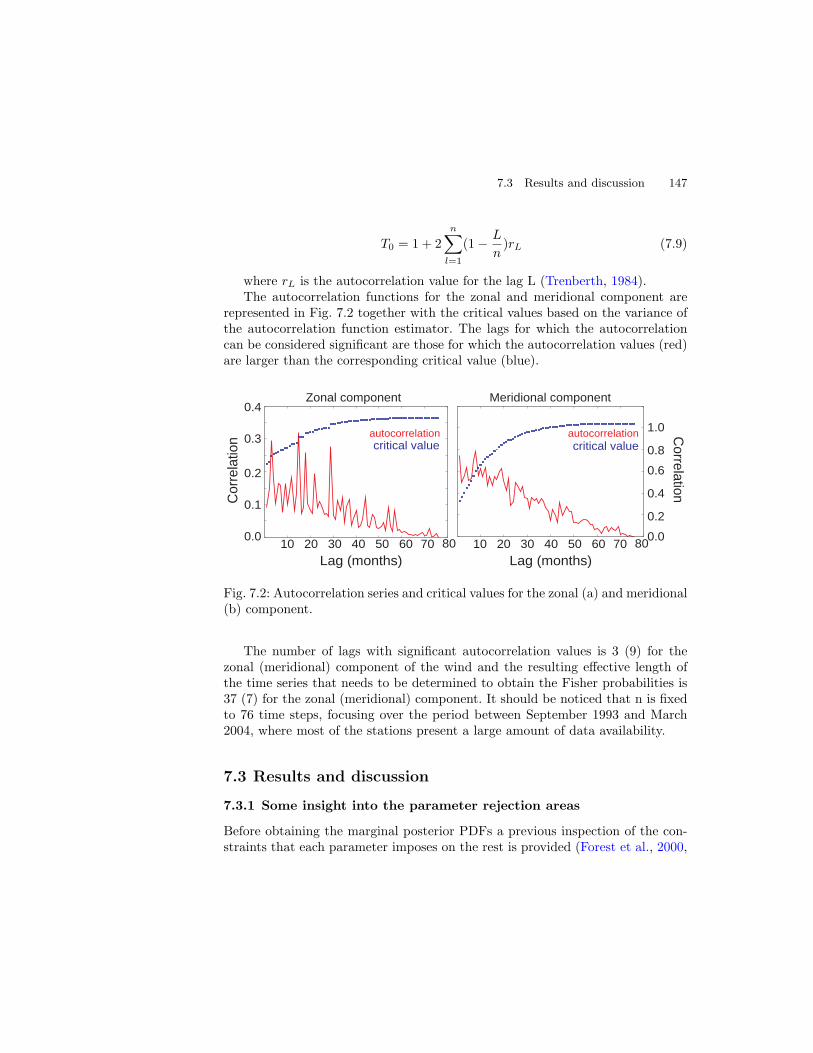
7.3 Results and discussion 147

T0 = 1 + 2n

∑

l=1

(1 − L

n)rL (7.9)

where rL is the autocorrelation value for the lag L (Trenberth, 1984).The autocorrelation functions for the zonal and meridional component are

represented in Fig. 7.2 together with the critical values based on the variance ofthe autocorrelation function estimator. The lags for which the autocorrelationcan be considered significant are those for which the autocorrelation values (red)are larger than the corresponding critical value (blue).

critical valuecritical value

Lag (months) Lag (months)

0.4

0.3

0.2

0.1

0.0

Co

rre

latio

n

Zonal component Meridional component

Co

rrela

tion

1.0

0.8

0.6

0.4

0.2

0.010 20 30 40 50 60 70 8010 20 30 40 50 60 70 80

autocorrelation autocorrelation

Fig. 7.2: Autocorrelation series and critical values for the zonal (a) and meridional(b) component.

The number of lags with significant autocorrelation values is 3 (9) for thezonal (meridional) component of the wind and the resulting effective length ofthe time series that needs to be determined to obtain the Fisher probabilities is37 (7) for the zonal (meridional) component. It should be noticed that n is fixedto 76 time steps, focusing over the period between September 1993 and March2004, where most of the stations present a large amount of data availability.

7.3 Results and discussion

7.3.1 Some insight into the parameter rejection areas

Before obtaining the marginal posterior PDFs a previous inspection of the con-straints that each parameter imposes on the rest is provided (Forest et al., 2000,

148 7 Bayesian uncertainty in downscaled wind field estimations

2002). With this aim a statistic R2 is calculated as the sum of squared residualsfor each estimated series weighted by the inverse of the minimum residual vari-ance (the estimations that show minimum variance of its residuals are selectedamong the whole set of estimations, see Appendix A). Then, the average R2 ob-tained for each pair of parameter values is represented for every combination oftwo parameters. The surface generated is suitable for discriminating which re-gions of the parameters space may be rejected based on the ability of each pairof parameters to provide estimations with small residuals. Parameter rejectionareas are plotted in Figures 7.3 and 7.4 for the zonal and meridional componentof the wind, respectively. Thus, as explained each map represents the ||r||2/σ2

rmin

of every pair of parameters values.The pattern in Fig. 7.3a represents for the zonal wind component the rejec-

tion areas based on the R2 statistic of µ vs. κ, i. e., the large scale domain (xaxis) vs. the number of EOFs/CCAs retained (y axis: numbers in the κ tripletsstand for the number of predictor EOFs, the number of predictand EOFs andthe number of CCA modes, respectively). It indicates that smaller values of R2

appear in the region of middle sized windows, that implies a better performanceof those model configurations that consider a medium size domain. The minimumis located along the domain number 5 (see Fig. 5.5). It can be appreciated thatpoor constraints are placed by the parameter κ, since R2 reaches similar valuesfor all κ possibilities. This is obvious for the larger domains (1-3). However, forthe smaller sizes of µ, some options of the number of EOF/CCA modes behavecomparatively worse. These values correspond to those cases where two CCAsare included in the model. It seems that the worst combination of κ is 222, theone that incorporates less number of EOFs and CCAs.

Similar behaviour could be observed when combining µ with σ (predictorfield) in Fig. 7.3b. Middle size windows perform better and larger windows per-form worse showing similar R2 values for all combinations of predictors. Smallerwindows (µ ǫ [7,9]) perform better only with some combinations: those includingthe wind components, U10 and V10 as predictors.

In the combination of σ and κ (Fig. 7.4c), those options of σ comprising U10and V10 present smaller values of R2, for all possibilities of κ. In addition, thosepredictor fields that generate small residuals maintain this tendency with everycombination of number of patterns, except with κ=222 that has larger residualsfor all cases. Then, it seems that is the predictor field who imposes strongerconstraints on the number of modes included in the model.

In the case of the combination of σ and θ (crossvalidation subset size) it canbe appreciated (Fig. 7.3d) that the latter does not produce constraints on thepredictor options. The cases that preset smaller residuals coincide with thosecases where the wind components are included as predictors. Thus if the predic-

7.3 Results and discussion 149

130

130

130

130

130

130

130

180

180

180

230

230

10

0 2

00

30

0 4

00

15

0

15

0

120

120

120

140

140

160

160

160

180 180

180

180180

200

200

200

200

200

220220

220220

220

220

10

0

V2 V4 V6 V8

322

433

532

552

633

653

z8-uv-t8

z8-t8

uv10

sl-z5-uv

uv-t8

2 4 6 8

130

130

130

130

130

130

190

190

190

250

250

370

10

0

µ (Large scale window) θ (crossvalidation opt)

V2 V4 V6 V8

µ (Large scale window)

κ (n

o E

OF

s p

rt,E

OF

s p

rd,C

CA

s)σ

(Pre

dic

tor

field

)

z8-uv-t8

z8-t8

uv10

sl-z5-uv

uv-t8

σ (P

redic

tor fie

ld)

155

155

15

51555

51

155

1555

51

55

1

155

155

155

15

5

205

205

205

55

2

120 1

80 2

40 3

00

2

4

6

8

θ (cro

ssvalid

atio

n o

pt)

κ (no EOFs prt,EOFs prd,CCAs)

140140

140

140

140140

140140

140

140

140

140

190

190

190

190

190

190

190 190

190

190

190

190

190

190240

240

240

240

240

240

240

240

240

240

240

240

240

240

240

290

290

290

κ (no EOFs prt,EOFs prd,CCAs)

322433532552633653

σ (P

redic

tor

field

)

z8-uv-t8

z8-t8

uv10

sl-z5-uv

uv-t8

118

118

138

138

158

158

178

178

198

218

V2 V4 V6 V8µ (Large scale window)

2

4

6

8 θ (cro

ssvalid

atio

n o

pt)

zonal wind componenta)

b)

c)

d)

e)

f)2

00

30

0 4

00

1

20

20

0 2

80

10

0

14

0

1

60

20

0

1

40

18

0

22

0

322433532552633653

Fig. 7.3: Rejection maps for each pair of parameters: a) domain-number ofmodes, b) domain-predictor, c) number of modes-predictor, d) crossvalidationsubset-predictor, e) number of modes-crossvalidation subset and f) domain-crossvalidation subset.

150 7 Bayesian uncertainty in downscaled wind field estimations

tor field generates small residuals, any option of the crossvalidation parameterperforms well.

The comparison between the number of modes (κ) and the crossvalidationoption (θ) indicates (Fig. 7.3e), as in the previous case, that the latter doesnot produce constraints on other parameters. It can be appreciated that thenumber of patterns presenting smaller residuals are those with four CCA patternsincluded, starting from those with the largest number of EOF patterns. Thecombinations presenting larger residuals are those that include only two CCAmodes.

The crossvalidation subset values do not generate constrains on the large scaledomain parameter as can be seen in Figure 7.3f. In general the performance of themethod is better with the middle size windows and the quality of the estimationsdecreases as the large scale domain enlarges or decreases.

For the case of the meridional component similar comments can be made.Additionally it is interesting to mention that the variability of residuals is larger(Figs. 7.4a-f). In the case of the number of patterns retained, there is a cleardivision of residuals, being smaller the cases with four CCA modes, followed bythe cases with three CCA modes and being the worst cases those with only twoCCA modes included (Fig. 7.4e). The stratification in the cases with 4 and 3modes was not so clear for the zonal component. The relation between domainand crossvalidation subset, reveals that the central windows perform generallybetter.

Thus, the analysis of parameter rejection areas based on the average residualsof each pair of parameter values allows to identify what parameter combinationsgenerate estimations with smaller residuals. In general, medium size domains,predictor field combinations including the 10 m wind components or the inclusionof more than two CCA modes seem to best fit the observed records. Overall thecrossvalidation parameter has little influence on the final statistics. This is adesirable result given the fact that θ is an exogenous parameter of the model.Stating that it does not have a discernible impact on the residuals is tantamountto saying that we are not modifying the evaluation of model skill by our decisionson the selected crossvalidation set up.

In the view of the constraints that each parameter imposes on the rest, it canbe said that the more relevant parameter is the size of the large scale window,followed by the predictor field and the number of EOFs/CCAs included. Thecrossvalidation parameter does not seem to be relevant for the skill of the model.These results are in agreement with those in Section 5.4.1. However the moreinteresting comment here is that this analysis has allowed for discriminatingwhich values of each parameter produces better estimations in terms of theirresiduals. This involves then further knowledge with respect to the frequentist

7.3 Results and discussion 151

V2 V4 V6 V8

322

433

532

552

633

653

z8-uv-t8

z8-t8

uv10

sl-z5-uv

uv-t8

2 4 6 8

µ (Large scale window) θ (crossvalidation opt)

V2 V4 V6 V8

µ (Large scale window)

κ (n

o E

OF

s p

rt,E

OF

s p

rd,C

CA

s)σ

(Pre

dic

tor

field

)

z8-uv-t8

z8-t8

uv10

sl-z5-uv

uv-t8

σ (P

redic

tor fie

ld)

12

0

18

0

24

0

30

0

2

4

6

8

θ (cro

ssvalid

atio

n o

pt)

κ (no EOFs prt,EOFs prd,CCAs)

κ (no EOFs prt,EOFs prd,CCAs)

σ (P

redic

tor

field

)

z8-uv-t8

z8-t8

uv10

sl-z5-uv

uv-t8100 140 180 2

20

V2 V4 V6 V8µ (Large scale window)

2

4

6

8 θ (cro

ssvalid

atio

n o

pt)

meridional wind componenta)

b)

c)

d)

e)

f)

120

120

120

120

120

150

150

150

150

150

150

150

150

180

180

180

180

180

180

180180

180

180

180

180

180

210

210

210

210

210

100 1

50 2

00 2

50

120130

130

140

140

150

150150

06

117

0180

190

200

210

100

100

100

130

130

130

130

160

160

160

160

190

190190

220

220

250

250

280

10

0 1

50

20

0 2

50

130

130

130

130 1

30

140

140

140

140

140

140

150

150

1501

50

150

150

150

150

150

150

150

160

160

170

170

170

180

180

08

1

180

09

1

125

125

125

125

125

125

125

145

145

145

165

165

165185

185

185

185

185

185

185

205

120 160 2

00

115

115

115

115

115

115

115

135

135

135

135

135

135

135

155

155155

155

155

155

155

155

155

155

175

175175

195

10

0 1

50

20

0 2

50

322433532552633653

322433532552633653

Fig. 7.4: As in Figure 7.3 but for the meridional component.

152 7 Bayesian uncertainty in downscaled wind field estimations

analysis as it provides an insight into the differentiated ability of each parametervalue of the downscaling model. These preliminary results are contrasted withthe more elaborated Bayesian approach in the following section.

7.3.2 Posterior distributions

The joint PDF of the data conditioned to the parameters (likelihood function) wascalculated on the basis of a Fisher distribution, combined with the correspondingprior uniforms to obtain a joint posterior distribution of each parameter. Theyare represented in Figs. 7.5 (Fig. 7.6) for the zonal (meridional) wind component.The posterior PDF for the large scale domain (µ) assigns the highest probabil-ities to the smallest windows sizes (µ=7-9, Fig. 7.5a and 7.6a), and penalizesthe rest with lower probabilities in the case of the domain number 5 and 6 andclose to zero for larger windows. Thus the Bayesian analysis identifies as suitablethose domains that cover smaller areas and rejects the rest. The marginal poste-rior for the predictor field (σ, Fig. 7.5b and 7.6b) selects those combinations ofparameters that include the U10 and V10 wind components of the wind (fromERA-40 fields) as predictors, specifying for them the highest probabilities, spe-cially for the cases with less number of fields included. Probabilities decrease asmore fields are incorporated as can be appreciated in Figs. 7.5b and 7.6b. ThePDFs for the number of EOF/CCA modes (κ) show a bimodal appearance (Figs.7.5c and 7.6c). The probabilities assigned to the parameters have been dividedinto two groups, those combinations of parameters with only two CCAs includedare labeled in the x axis with the numbers 1-15 and the rest (those includingthree or three and four CCA modes) are designated with numbers between 16to 31. The probability distribution indicates that in general the combinations ofparameters with only two CCAs receive lower probabilities. Higher probabilityvalues are shown for the combinations with four CCA patterns followed by thosewith three. However there is a subgroup of combinations in the area of only twoCCAs (12-15) that show probabilities comparable to the cases with four CCAs.The zonal and meridional component PDFs show very similar information withthe exception of a division between three and four CCAs not so clear in the zonalcomponent as with the meridional one. The marginal PDF for the crossvalidationsubset size (θ) reveals very similar probabilities for all parameter values, with theonly exception of the subset 5 (5 months) of the zonal component (Fig. 7.5d) andthe last two options corresponding to the subsets 8 (14 months = 2 years) and 9(28 months = 4 years) of the meridional component (Fig. 7.6d), which show verylow probability.

Through the Bayesian inference on the model parameters based on themarginal posterior distributions we have arrived at two different situations. On

7.3 Results and discussion 153

N EOFs/CCAso

5 10 15 20 25 30

Crossvalidation subset size

1 2 3 4 5 6 7 8 9

Pro

ba

bili

ty d

en

sity

Pro

ba

bility

de

nsity

Large scale domain Predictor field1 2 3 4 5 6 7 8 9 1 5 9 13 17 21 25

0.30

0.25

0.20

0.15

0.10

0.05

0

0.07

0.06

0.05

0.04

0.03

0.02

0.01

0

0.16

0.12

0.08

0.04

0

0.14

0.13

0.12

0.11

0.10

0.09

0.08

Fig. 7.5: Marginal posterior distributions of the zonal component of the windfor a) the large scale domain (µ), b) the predictor field (σ), c) the number ofEOF/CCA patterns (κ) and d) the crossvalidation subset size (θ).

one hand we have found consistency with results from the parameter area rejec-tion analysis in the case of the crossvalidation subset: both indicates that thereare little differences between the various options considered for this parameters interms of the residuals of estimations, except for the case 5 (8 and 9) of the zonal(meridional) wind component. In addition for the predictor field, both analysesresolve that there is a positive impact on estimations when including as predic-tor the wind components, U10 and V10. However, the marginal PDF penalizesconsiderably the rest of combinations, pointing out that the rest of parameterscombinations should be rejected. On the other hand a lack of agreement is evi-dent for the other two parameters: the marginal PDF of the large scale domainevidences penalization for the middle size windows being the smaller ones re-warded. For the number of EOF/CCA modes although smaller probabilities alsocorrespond to the case with only two CCAs, a high score is shown in three cases(κ=622, 522, 422).

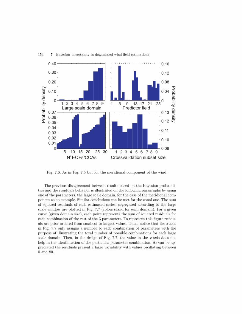
154 7 Bayesian uncertainty in downscaled wind field estimations

Probabilitydensity

Large scale domain

N EOFs/CCAso

5 10 15 20 25 30

Crossvalidation subset size

1 2 3 4 5 6 7 8 9

Predictor field1 2 3 4 5 6 7 8 9 1 5 9 13 17 21 25

0.07

0.06

0.05

0.04

0.03

0.02

0.01

0

0.16

0.12

0.08

0.04

0

Probability

density

0.13

0.12

0.11

0.10

0.09

0.30

0.20

0.10

0

0.40

Fig. 7.6: As in Fig. 7.5 but for the meridional component of the wind.

The previous disagreement between results based on the Bayesian probabili-ties and the residuals behavior is illustrated on the following paragraphs by usingone of the parameters, the large scale domain, for the case of the meridional com-ponent as an example. Similar conclusions can be met for the zonal one. The sumof squared residuals of each estimated series, segregated according to the largescale window are plotted in Fig. 7.7 (colors stand for each domain). For a givencurve (given domain size), each point represents the sum of squared residuals foreach combination of the rest of the 3 parameters. To represent this figure residu-als are prior ordered from smallest to largest values. Thus, notice that the x axisin Fig. 7.7 only assigns a number to each combination of parameters with thepurpose of illustrating the total number of possible combinations for each largescale domain. Then, in the design of Fig. 7.7, the value in the x axis does nothelp in the identification of the particular parameter combination. As can be ap-preciated the residuals present a large variability with values oscillating between0 and 80.

7.3 Results and discussion 155

In such conditions the shape of the Fisher distribution becomes of relevancesince a narrow distribution allows only for a few valid residual values, penalizingthe rest with lower or close to zero probabilities. Such a case corresponds toa very strict likelihood function which focuses on (assigns a high probabilityto) those combinations of parameters that produce the smallest residuals, i. e.,those cases for which the sum of squared residuals is very close to the minimum(see likelihood function design in the Appendix A). The latter situation canbe appreciated in Fig. 7.1 where the likelihood function based on the Fisherdistribution assigns close to zero or zero probabilities to most sum of squaredresiduals, and thus, to most of the parameter combinations. On the contrary, awider distribution would assign a probability different from zero to several sumof squared residuals allowing for the corresponding parameter combinations tobe considered as suitable configurations of the statistical model.

The shape of the Fisher distribution depends on its number of degrees of free-dom. This is determined by the number of parameters that needs to be tested andthe effective length of the estimated time series (specifically the estimate withminimum residual variance, see Section 7.2 and Appendix A). Some authors pro-pose a correction based on the serial autocorrelation in the attempt of generatingwider Fisher distributions (Hegerl et al., 2006). However, even with the correc-tion due to the autocorrelation, here the Fisher PDF or likelihood function isconsiderably slim as appears in Fig. 7.1. Nevertheless, in the view of the dis-agreement between results through posterior PDFs and parameters rejection inSection 7.3.1, the question arises whether the large amount of parameter combi-nations with low or very low probabilities should indeed be rejected as inadequateor less appropriate model set ups.

Two different behaviors deserve a comment in Fig. 7.7. On one hand, forthe approximately 3.000 parameter combinations with the smallest residuals ofeach large scale domain, it is possible to identify that systematically the largerwindows (see legend) generate larger residuals while for the medium and smallwindows residuals are smaller. Additionally, for the larger domains residuals aremore sparsely distributed whereas intermediate/small domains are less scatteredand concentrated around similar residual values. Still it can be appreciated thatresiduals for windows 7-9 are slightly lower than the corresponding to the cases5 and 6. On the other hand, the rest of parameter combinations (those with x >3.000) depict a more complicated behavior: the four smallest domains (numbers9, 8, 7 and 6, see Section 5.4.1) show a sudden increase of residual values forthe rest of combinations of parameters while residuals for domains 1 to 5 remainfairly stable or show a slight monotonous increase through the whole range ofcombinations.

156 7 Bayesian uncertainty in downscaled wind field estimations

In view of the latter it can be said that larger windows produce the largestresiduals between observed and estimated series while the small and intermedi-ate domains produce smaller residuals. However, only the middle sized windowsevidence a stable behavior: they show similar residuals for almost all possiblecombinations. In contrast, the smallest windows behave inadequately (very largeresidual values) for a large amount of parameters combinations. Nevertheless,even though it only happens for very few combinations of the statistical model,the minimum squared residual sums are attained when using the smallest do-mains number 8 and 9.

Consequently, the suitability of the different possible model configurations canbe then thought of in terms of two possibilities: either identifying the optimalcases, i.e., those with residual values close to the minimum whatever the behaviorwith the rest of parameter combination is (smallest window sizes) or recognizingthe cases with reasonably small residual values that systematically maintain thisbehavior with the greatest amount of model parameter combinations. The latteris not discriminated by the Bayesian approach that instead tends to identify thecases whose residuals are very near to the minimum (optimal cases) rejectingthe rest. The reasons for this are connected with the arguments given aboveabout the width of the likelihood function and its tendency to severely penalizecombinations of model parameters that generate residuals not rigorously close tothe minimum.

Number of parameter combinations

Sum

of square

d r

esid

uals

0 1000 2000 3000 4000 5000 6000 7000

100

80

60

40

20

0

Fig. 7.7: Sum of square residuals segregated according to the large scale domainfor the meridional component of the wind.

7.3 Results and discussion 157

A similar argument can be used to explain why some cases including only twoCCAs have obtained a high probability (not shown): for a few combinations ofthe rest of parameters, the smallest residuals are achieved by these three optionsmentioned: κ=622, 522, 422. As in the case of the large scale domain, this behavioris not stable for all the combinations of the rest of parameters and the residualsincrease considerable for many other combinations, especially for the smallestpredictor windows (7, 8 and 9; not shown).

These results hint a discussion about the interpretation of the Bayesian infer-ence regarding the degree of subjectivity that may be involved in every method-ology. The Bayesian method applied to the particular issue of determining thesuitability of the parameters in the model configuration is able to recognize someoptimal parameter combinations based on the residuals obtained between esti-mations and observations. However it failed in recognizing those parameters thatperform adequately with most of the combinations. The identification of thosecases is a desirable feature of the methodology since it would evidence thosemodel configurations that are more robust to changes in any of the other pa-rameter options. Thus, the Bayesian methodology may evidence skill dependingon the specific purposes of the analysis: for the detection of optimal cases withsmaller residuals, this method has shown efficiency in isolating the particularcases that minimize the error. If the aim is to determine stable combinations ofthe parameters for the identification of configurations that perform reasonablywell in most cases, the Bayesian approach as implemented here is partly limited.

Summarizing, the large scale windows that have shown a reasonable goodperformance with the rest of the parameters are the medium size ones whichinclude the large scale gradients that bring predictability for the regional wind.Too small windows, although not systematically, as we have seen for some combi-nations of parameters, can involve a loss of information regarding the large scaleatmospheric structure. The number of EOF/CCA modes has shown a segrega-tion of cases based on including or not the third and/or the fourth CCA modein the analysis (recall probabilities in posterior PDFs in Figs. 7.5c and 7.6c, forthe zonal and meridional wind component, respectively). Such a performance ofthis parameter is more evident in the cases based on using the smaller large scaledomains (see parameter rejection maps of Figs. 7.3a and 7.4a). Then, it can beconcluded that small windows with the minimum number of CCAs lead to apoor representation of the relations between the large scale flow and the regionalfeatures of the wind field. For the predictors there are clear advantages of usingthe wind components (posterior probabilities in Figs. 7.5b and 7.6b) althoughit cannot be said that the cases which do not incorporate U10 and V10 fail inreproducing the regional wind variability (Figs. 7.3b and 7.4b).

158 7 Bayesian uncertainty in downscaled wind field estimations

One more comment deserves attention at this stage. In Chapter 5 it was shownthat combinations of model parameters including only two CCAs produced esti-mations with a different tendency and sign (anomalies) than those that includedthree or more CCA. In this chapter both, the assessment based on the param-eter rejection areas and the Bayesian inference, agree in considering a better fit(smaller residuals for most of the parameter combinations) and a more robustbehavior (higher probabilities) in the cases including more than two CCAs. Al-though the reasons for this are still not clear and further investigation would beneeded to provide a physically meaningful argument, there are some evidencespointing out that the most suitable number of CCA modes in the downscalingmodel are those generating positive (negative) zonal (meridional) wind anomaliesin the reconstructions of Fig. 5.13. It is interesting to notice that the frequentistapproach for the uncertainties in Chapter 5 was not able to identify such dif-ferentiated performance of this parameter options (nor in the case of the otherparameters). This fact then illustrates to some extent the added value of thealternative approach proposed in this chapter.

An analysis encompassing the study of parameter-rejection areas and theBayesian posterior probabilities, has served as a mean to illustrate the adequacyof the different parameter values of the model set up. The former is based onthe average behavior of the residuals of each combination of parameters whilethe latter combines prior knowledge with a penalizing function (likelihood). Thefollowing subsection is devoted to discuss the role of the prior knowledge inthe performance of the Bayesian methodology. Thus, another question arisesregarding the sensitivity of the Bayesian method to changes in the assumptionsmade for the prior distributions. The robustness of the method is also assessedin the next subsection by exploring the spatial variability of the results from theBayesian analysis.

7.3.3 Sensitivity to prior knowledge

To gain insight into in the results achieved or to further learn about possiblecritical aspects of the methodology there is a need for examining also the abilityof the model to generate robust posterior inference when different prior distri-butions are used. For every parameter, the uniform PDF was substituted byanother prior PDF, where the probabilities were assigned by weighting the dif-ferent parameter values according to the residuals they generate: the larger thesum of squared residuals, the lower the probability, being this case representativeof a more realistic assignment of probabilities. With this the analysis starts at adifferent state of knowledge that could have implications in the final posteriors.Nonetheless, after the change of the prior distributions no variations in the finalposteriors distribution are appreciated. This is illustrated in Figs. 7.8b and 7.8g.

7.3 Results and discussion 159

In this figure left panels correspond to the sequence of different prior distribu-tions tested and right panels show the resulting marginal posterior of the largescale domain for the zonal component of the wind (similar results were found forthe meridional one). The first pair of plots (Fig. 7.8a and 7.8f) corresponds tothe case explored in the previous paragraphs where the prior distribution of allparameters was assumed as uniform. Further, various subjective priors have beenadditionally included in this sensitivity analysis to illustrate what are the thresh-olds in the prior information that are able to modify the posterior probabilities(Figs 7.8c-e). This is shown only for one parameter (the large scale domain) andfor the zonal wind component as an example. The prior distributions sequentiallyattach a higher probability to the medium size windows while the probability ofthe larger ones decreases. This sensitivity check illustrates how the posterior PDFis only able to show a change in the ’winner’ values of the parameter when theprior designates nearly zero probabilities to the smaller windows. As it can be ap-preciated in Fig.7.8 the changes in the prior assumptions only produce an impactin the posterior PDF when the probability assigned to the medium size windowsare close to 1 and subsequently the other probabilities are close to 0.

The latter implies that the determinant factor in the analysis is the likelihoodfunction which ultimately decides the posterior probabilities. Other authors usedifferent approaches for the modelling of the likelihood function, employing Gaus-sian distributions to penalize the residuals (Jackson et al., 2004), or in other stud-ies, some more sophisticated diagnostics of the goodness of the fit by the model(Coelho et al., 2004). However, apart from an examination of the technical de-tails of the approach, the interesting point here is to notice that an objectiveapproach like the Bayesian one as exposed here, also needs a detailed analysis ofits performance and a thorough review of the various assumptions made in thedesign of the strategy in order to interpret the results obtained.

To finish, an additional test is carried out with the twofold aim of understand-ing more on the robustness of the method and to discern some aspects regardingthe spatial variability of the methodology. Thus a similar Bayesian analysis asimplemented for the regional wind estimations is accomplished at every locationwithin the dataset and for each one of parameters. The large scale domain poste-rior PDFs at every site in the CFN are represented in Fig. 7.9 for the meridionalcomponent of the wind. In view of the posterior distributions it can be said thatin most of the locations there is a tendency for assigning the highest probabilitiesto the smaller windows and lowest (nearly zero) to the medium (large) domainsizes. In this sense the method is robust. However, it can also be appreciatedthat at a few sites the dominant contribution to the PDF is given by windowsnumber 5 or 6 revealing a partial disagreement between the different time series.However no spatial pattern can be associated to the fact that some of the stations

160 7 Bayesian uncertainty in downscaled wind field estimations

Large scale domain size

Pro

ba

bili

ty

Pro

ba

bility

0.2

0.15

0.10.2

0.1

00.3

0.2

0.1

00.8

0.6

0.40.2

0.60.40.2

0

0.4

0.3

0.20.10

0.4

0.3

0.2

0.100.50.40.30.20.10

0.7

0.5

0.3

0.1

0.8

0.6

0.4

0.2

01 2 3 4 5 6 7 8 91 2 3 4 5 6 7 8 9

1.00.8

a)

b)

c)

d)

e) j)

i)

h)

g)

f)

Fig. 7.8: Left: Different µ prior distribution tested for the estimations of the zonalwind component. The weights that are assigned to the medium size large scaledomains are progressively increased while the corresponding to the other windowssizes are decreased. Right: marginal posterior µ PDFs obtained by applying thecorresponding prior PDF.

7.4 Conclusions 161

present a differentiated behavior of the posterior PDFs: the sites whose marginalPDF assigns higher probabilities to the middle windows cannot be segregatedaccording to a division in subregions, nor they can be divided depending on theability of the method at each station to generate reliable estimations (see Fig.5.4). It can only be mentioned that some of those specific stations are locatedalong the Ebro Valley or in mountainous sites. This hints a good exposure to thecirculations, not intensively affected by the local features that could be associ-ated with the fact of detecting as more appropriate the medium size domains toprovide a suitable representation of the atmospheric structure and the large scalegradients that are important for the regional wind predictability. For the case ofthe predictor field (not shown) apparently all the locations tend to show a pre-dominant influence of the combinations including the U10 and V10 componentsof the wind. In the case of the number of modes a spatial distribution cannotbe found neither, as in the case of the parameter µ. The map shows a similartendency as in the regional case exposed in Figs. 7.6 and 7.7. Thus, it seems thata change of the time series that are the inputs of the method (i. e., whether theyare the regional or the local estimates) does not produce a great impact in theresults.

7.4 Conclusions

In this chapter a complementary approach to the frequentist evaluation of themethodological uncertainty associated with the use of a single downscaling modeland multiple configurations has been presented. This is done by exploring theproperties of the model parameter probability distributions. Thus, the assessmentof the methodological sensitivity presented herein was focused on providing aprobabilistic analysis on the suitability of parameter values to yield wind fieldestimations in good agreement with the observations, rather than presentinga measure of the methodological variability of wind estimates as in Chapters5 and 6. The methodology raised is based on a Bayesian probabilistic analysisthrough which prior knowledge on the parameter population is combined with theavailable observations to generate posterior distributions. This posterior PDFsallow for making inferences about the ability of the different parameter optionsto produce skillful estimations.

The parameters of the model set up that were tested through this method-ology are the size of the large scale domain, the predictor field(s), the numberof EOF/CCA modes to be retained and the crossvalidation subset size. Uni-form prior distributions were used in a first step allowing for equal probabilitiesto each parameter value. In addition, a likelihood function responsible for pe-nalizing those configurations that generate estimations with large residuals was

162 7 Bayesian uncertainty in downscaled wind field estimations

Large scale domain

Pro

bab

ilit

y

Fig. 7.9: Marginal posterior PDF of the large scale domain at each locationwithin the CFN for the meridional component of the wind.

calculated based on the Fisher distribution. The formulation of the approach ex-posed in this chapter can be considered an interesting contribution since a fullelaboration of the theoretical aspects leading to a likelihood function based onthe Fisher distribution selection is not totally documented in the literature.

Previous to the analysis of the marginal posterior PDFs of each parameter,the constraints that a parameter imposes on the others were evaluated by calcu-lating the parameter rejection areas, where a statistic R2 was calculated, for everypair of values of each two parameters, based on the residuals. This examinationallowed for a segregation of the model parameter options that on average providemore skilled wind estimates. It was found that using 10 m wind components aspredictor fields, including more than 2 canonical modes in the downscaling model

7.4 Conclusions 163

or selecting the intermediate sized large scale windows rendered estimates withsmaller residuals with respect to the observations and thus, those can be con-sidered the more suitable parameters in the model set up. However, the resultsfound in such an approach are not substantiated for the posterior marginal distri-bution of all parameters. Disagreements were found in the case of the large scaledomain, for which the rejection areas suggested that the medium size windowswere the most suitable for the downscaling exercise whereas the Bayesian infer-ence rejected this domain sizes in favour of the smaller ones. In the case of thepredictor fields both assessments agreed in considering as better configurationsthose cases that incorporate the components of the large scale wind field. How-ever, the Bayesian analysis assigns a very low probability to the rest of predictorfield options although estimations of quality are also found in those cases. Thenumber of EOFs/CCAs in both cases evidences a better skill in generating esti-mations of those combinations of parameters incorporating more than two CCAmodes. However, also a few cases with only two CCAs receive high probabilities inposterior distributions of the Bayesian analysis. In the case of the crossvalidationoptions both, rejection areas and Bayesian posteriors hint to similar probabilitiesfor all possible values.

The disagreement between both types of analysis has been found to be relatedto the average behaviour of the residuals (that is calculated in the parameterrejection areas approach) in contrast with the tendency of the Bayesian approachto assign high probabilities to the optimum configurations (residuals close to theminimum) and rejecting the rest of the configurations. The reasons for this werefound to be related to a narrow and thus, strict Fisher distribution that servedas the likelihood function in the Bayesian approach.

Different prior distributions were tested for the case of the large scale do-main parameter in order to understand the sensitivity of the Bayesian method tovariations in the prior knowledge. Priors were successively modified by increas-ing the probabilities of those options that showed a reasonable performance interms of residuals for most of the combinations of parameters. No influence in themarginal posterior PDFs were detected unless the prior were forced to overweightsome cases, for instance intermediate sized windows, with very high probabilities.Thus, the responsible for such a severe judgement of the performance of the dif-ferent model configurations in the Bayesian approach is apparently the likelihoodfunction that focuses on the optimal cases and assigns close to zero probabilitiesto the rest.

The focus of applying this Bayesian formal technique was to isolate the ro-bustness of some model configurations in generating realistic estimations in orderto further constrain the previous frequentist selection of possible parameter val-ues, that was based on more heuristics arguments (Chapters 5 and 6). However,

164 7 Bayesian uncertainty in downscaled wind field estimations

the methodology returns solely the optimal configurations based on the mini-mum residuals, i.e., instead of identifying the more robust model set ups, theprobabilistic model detected rather a few optimal configurations. In contrast, theevaluation of the parameter rejection areas, based on the behavior of the av-erage residuals, provides in this particular case an appropriate response to themain question: the search of the parameter options that produce estimations ingood agreement with observations and are robust to changes in any of the restof parameter values of the model configuration.

8

Conclusions and discussion

Humanity needs practical men, who get the most out of their work, and, without

forgetting the general good, safeguard their own interests. But humanity also

needs dreamers, for whom the disinterested development of an enterprise is so

captivating that it becomes impossible for them to devote their care to their own

material profit. Without doubt, these dreamers do not deserve wealth, because

they do not desire it. Even so, a well-organized society should assure to such

workers the efficient means of accomplishing their task, in a life freed from

material care and freely consecrated to research. [...] Nothing in life is to be

feared. It is only to be understood.

M. Curie, Autobiographical Notes, 1867-1934

This work aimed at providing an improved understanding of the variability ofthe wind field, and its derivative, the wind power production, at regional scales0n the basis of their connection with the large scale atmospheric variability.Thus, two different, though related lines have been explored in this work. Inthe first part of the study the relationships between the wind speed and thewind power generated at various wind farms over a complex terrain region in thenortheastern Iberian Peninsula have been examined. In the second part of thetext the variability of the wind field measured at some stations in the same regionhas been investigated by identifying the main connections between the local windat the CFN and the large scale atmospheric circulation over the North Atlanticarea. Finally, the two parts have been assembled by exploring the link betweenthe wind power production variability and North Atlantic atmospheric circulationin the basis of the wind-wind power relation evidenced in the first part. Themethodological uncertainty associated with wind and wind power estimationshas been explored throughout the various chapters of the second part of themanuscript.

166 8 Conclusions and discussion

The specific conclusions found in the different analyses of this work weredetailed in the corresponding section at each chapter. From a broader perspective,the main conclusions of this Thesis are summarized and discussed in Section 8.1.An insight into the open questions and a brief discussion about some concernsrelated to different aspects within the Thesis are discussed in Section 8.2 andSection 8.3.

8.1 Conclusions

The theoretical PDF traditionally used to represent the wind speed population(Weibull distribution) does not reproduce at every location the properties of theobserved wind. This lack of agreement between theoretical and observed wind dis-tributions does not produce however a severe impact on the Weibull based windenergy estimations due to a partial cancellation of errors in the calculation ofthe wind power estimation. This exploration was raised on the basis of a criti-cal evaluation of classical assumptions in the representation of the wind speedempirical distributions at hourly timescales and allowed for a quantification andunderstanding of the errors in the wind power estimations arising from the as-sumptions made on the probability distribution of the wind speed.

A linear empirical relation was evidenced between the wind speed and the windpower at monthly timescales while at shorter timescales the wind power is a func-tion of the cubic wind speed. This evidence has proven a decisive bearing in theevaluation of the relations between the wind energy variability and the atmo-spheric circulation at monthly time scales in the second part of the work andis derived from the comparison of several methods that made use of hourly ormonthly resolution to estimate wind energy production. Simpler methods gen-erally perform well in comparison with more elaborated strategies that requirehigher temporal resolution data. Notwithstanding, all methods reproduce to alarge extent the temporal variability of the observed wind power. Additionally,the quantification of errors in wind power estimations led to identify a largercontribution to these errors due to the assumptions in the wind-wind power re-lationship compared to that related to the representation of the wind by theWeibull probability distribution.

A considerable fraction of variance of the regional wind field over the CFNcan be attributed to the large scale atmospheric variability over the North Atlanticarea. The main modes of covariability between the local wind and the predictorfields, found by means of the application of a statistical downscaling technique

8.1 Conclusions 167

(CCA), showed substantial contributions from the East Atlantic/Western Rus-sian and East Atlantic teleconnection patterns. The analysis also evidenced therole of the orography in the region that gives raise to the regional circulationsfound: typical up and down Ebro Valley regimes and more complicated circu-lations in the central and northern areas of the region. To our knowledge noreferences in the literature could be previously found regarding a statistical down-scaling of the wind field over the IP. Results have supported the inspection, ina subsequent part of the study, of links between the North Atlantic atmosphericvariability and the regional wind power production at the CFN. The founda-tions for such an exploration are based on the linearity between the wind powerand the wind field, and between the latter and the large scale circulation changes.

The uncertainty in the wind field estimations associated with the method-ological variance reasonably preserved the variability of wind observations andthus, the statistical method proved robust to changes in the model configuration.The analysis showed that the methodological sensitivity is largely dependent onthe variability of the wind: those locations with larger variate evidenced a largesensitivity to variations in the model configuration. In addition, no differentialimpacts on the estimations of any of the parameters involved in the model setup were identified at this step. This circumstance motivated, in the last partof the work, a probabilistic assessment of the methodological uncertainty thataimed at imposing further constraints to the multiple model configurations in or-der to identify those with a superior skill in generating suitable wind estimations.

Large interannual as well as interdecadal variability was evidenced in the re-construction of the wind field during the last centuries. The assessment of themethodological uncertainty at long timescales showed an interesting impact onpast wind estimations due to changes in the model set up: the inclusion/exclusionof a certain canonical mode produced a bias to positive/negative estimates. Thisimplication of the model configuration choice was not detectable during the ob-servational period and then it contributed to stress the need of considering withcaution estimations from any single model configuration. For this period, no cen-tennial trends were appreciable although some episodes of anomalous large windspeeds were identified connected with low frequency changes of the relevant largescale modes over the North Atlantic region. Knowledge regarding variability froma broader perspective of past long term changes may have relevant applicationsin the understanding of, for instance, future variations of the wind field in thecontext of climate change regional projections.

168 8 Conclusions and discussion

The linearity between the monthly wind and the large scale circulation can beextended to the wind power. Thus, the regional variability of the wind power gen-erated at several wind farms within the CFN can be partly attributed to variationsof the relevant large scale modes in the region, as in the case of the wind field.The main mode of covariability between predictand and large scale predictors issimilar to the second principal canonical pattern found during the downscalingof the wind field. Hence, results from the downscaling of wind power productionwere robust with those obtained for the case of the wind speed. Results from com-parisons among a set of methodological variants that made use of the downscaledwind field and transfer linear functions to obtain final wind energy estimates, re-vealed that the direct downscaling performs generally better than the rest. Theseapproaches proved useful to provide wind power production estimates in areaswith no availability of power data and also for periods out of the observationalone. This served as illustration of potential and simple applications providinginformation of the available wind power over a wider region and for longer thanthe observed periods with low computational efforts. The spread of the ensembleof estimations obtained in the methodological uncertainty inspection comprisedmost of the wind power observations, showing a comparable sensitivity as thewind field to changes of the model parameters.

Certain parameters of the downscaling model configuration evidenced a com-paratively larger ability with respect to the rest within the parameter space toprovide reliable wind estimations. A procedure that imposed constraints to theparameters performance based on the residuals identified that including the windcomponents at 10 m as predictor fields or more that two CCA patterns in thedownscaling model and using the middle size large scale domains implies somebenefits for obtaining estimations in good agreement with observations. However,the subsequent Bayesian analysis, that allowed for inferences on the posteriorprobability distributions of the parameters of the statistical model, exhibited somediscrepancies with the previous result. The arguments for this discrepancy pointedto the ability of the Bayesian analysis for discriminating the optimal configura-tions but its difficulty to identify those parameter values that provide reliableestimations with most of the possible model configurations, whatever the valuesof the rest of parameters are. Such a difficulty was directly connected with theextremely narrow likelihood function that penalizes with nearly zero or very lowposterior probabilities all cases whose residuals were not very close to the min-imum. This approach has not yet been extensively applied for the estimationsof regional climate variability and further investigations would be required tounderstand the implications of the various assumptions in the methodology.

8.2 Quo Vadis? 169

8.2 Quo Vadis?

The statistical downscaling approach considered for this work is focused onmonthly timescales. This allowed for concentrating on the variations of the windfield that to a great extent are related to variations of the large scale atmo-spheric circulation. Thus, the local processes that typically are resolved at shortertimescales are not considered for this analysis that focuses mostly on the regionalsignal. However, increasing the temporal resolution may be of use for instance,in the context of impact studies and extreme events assessment that may requirehigher spatial and temporal resolution (Maurer and Hidalgo, 2007).

An evaluation of the daily wind field predictability would provide insight intothe ability of the statistical downscaling technique applied here for reproducingthe observed daily variability. References in the literature regarding statisticaldownscaling of daily temperature and precipitation related variables are frequent(Wilby, 1998; Huth, 2002; Huth et al., 2008; Hundecha and Bardossy, 2008;Wetterhall et al., 2009), but the topic has been less addressed within a focus onthe wind field. Then, such an analysis would deserve special attention.

A related issue regards the question whether other methodologies (i. e., nonlinear methodologies) would reproduce the regional wind variability compara-tively with the CCA. A survey of methods that can empirically relate local toglobal climate variables can be cited so far: analog methods, fuzzy logic, weathergenerators, compositing, neural networks, etc. (Wilby and Wigley, 1997; Wilbyet al., 1998). Analog methods, for instance have proven efficiency in reproducingthe daily and monthly local precipitation picking up the proper level of observedvariance (Zorita and von Storch, 1999; Fernandez and Saenz, 2003) while perform-ing as well as more elaborated multivariate approaches like the technique appliedin this work. In contrast, the last type of approaches can provide a clear physi-cal interpretation of the cross-scale relationships found. Further investigations onthese issue would involve an understanding of the drawbacks and advantages ofmethodologies in the field of statistical downscaling approaches, that, to a greatextent remain a challenge in the case of wind related variables.

In this line, a pertinent question can be posed regarding the comparison ofboth statistical vs. dynamical downscaling models applied to reproduce the re-gional wind field variability. The study by Jimenez et al. (2010b) produced aRCM simulation over the same target region as in this work. The WRF (Ska-marock et al., 2005) model simulation covered the whole observational period(1992-2005) at 2 km of horizontal resolution. The evaluation of the model abilityto reproduce the variability of the wind field was carried out at daily timescales.Here the regional simulated time series from WRF and CCA estimations are com-pared at monthly timescales. Series are represented in Fig. 8.1a,b for the zonal

170 8 Conclusions and discussion

and meridional component of the wind, respectively, together with the observa-tions.

a)

b)

Time (year)Me

rid

ion

al w

ind

an

om

alie

s (

m/s

)Z

on

al w

ind

an

om

alie

s (

m/s

)

WRF simCCA estsObservations

2

1

0

-1

-2

2

1

0

-1

-2

2

-1

2

1

0

-2

-3

-4

1992 1994 1996 1998 2000 2002 2004 2006

Fig. 8.1: Regional series of the observed (dashed blue) zonal (a) and meridional(b) wind components at the CFN compared to the CCA estimates (light blue)and the WRF simulation at 10 m (black).

As it can be observed in the plot, both estimations reproduce the regionalvariability of the wind components. In general the WRF simulation tends to re-turn higher variance than the CCA estimations, but it is also noticeable thatfor some time steps the WRF model overestimates the observed variance. Thereare also situations in which neither the CCA nor the WRF can simulate thecorrect variability. Notwithstanding the main issue here is to provide a first ap-proximation to the relative performance of both methodologies that reproduce

8.2 Quo Vadis? 171

with similar ability the observed regional wind field. This a preliminary insightinto the relative skill of each method to obtain estimations of the wind field overa complex terrain region. Further analyses would be necessary to evaluate thedrawbacks and advantages of each approach.

In fact, one of the main concerns when applying empirical methods, in com-parison with dynamical ones, for the downscaling of climate variables is the non-stationarity of the relation between spatial scales. An important assumption ofthe empirical downscaling methods is that the relation between the global circu-lation and the regional scales holds in a perturbed climate (Benestad, 2002). Thelater cannot be guaranteed and thus, this is also catalogued as the main drawbackof these models. Some studies have assessed the presence of non-stationarities inthe empirical relations between the atmospheric dynamics and the local climatevariability. They have found evidences in both directions: while, for instance, He-witson and Crane (2006) and Schmith (2008) identified signals of non-stationarityover the training period of the model, others, as Murphy (1999) and Hanssen-Bauer et al. (2003), found no indications of significant non-stationarities. To agreat extent a reasonable expectation for altered future states of the climate isthat they will involve changes in the intensity, frequency of occurrence and persis-tence of the large scale atmospheric patterns (Hewitson and Crane, 1996). Underthis logic, further uncertainty will arrive to regional future projections but thiswould not necessarily invalidate the conceptual approach that aims at identifyingthe empirical relations between large and regional/local scales.

Through the assessment of the long term variability of the regional wind fieldin this work it has been evidenced that there are signs of an influence of the non-stationarities in the intensity of the associations between the large and the localscales on the variability of the wind at decadal and centennial timescales. Thisfinding was based on assessment of the methodological sensitivity involved inthe downscaling procedure. This fact highlights the importance of exploring thesources of uncertainty which is crucial for evaluating the reliability of estimations.An interesting assessment would involve a sensitivity analysis to variations in theintensity of the associations between global and regional scales and their impacton wind estimations during the calibration period. The approach can be put inthe context of the generation of regional climate change scenarios. The intensityof the associations found during the observational time interval may be artificiallyincreased/decreased creating an ensemble of potential situations and their impacton the estimations uncertainty could be evaluated. Subsequently this could beextended to the past and future estimated variability of the regional wind toexamine the importance of this variations in periods different to the observationalone.

172 8 Conclusions and discussion

Regarding the long term regional variability, the question that naturally arisesfrom the analysis carried out here would regard the estimations of the wind fieldand the wind power production in future climate change scenarios. The mainissues to address in this context are the comparative variability of the wind fieldin the future with respect to that during the last centuries. An assessment ofthe estimated future changes of wind speed and wind power variables could befeasible by using the different available GCM simulations over the twenty firstcentury. Whether long term trends may appear or the agreement between estima-tions based on different GCM simulations leads to reliable projections are someof the interesting issues to focus on. Moreover, changes in the frequency of occur-rence or intensity of those large scale circulation modes that are responsible forthe observed wind and wind power regional variability and the impact in futureregional projections of focusing in different climate change scenarios can be ex-plored. Further, this exercise poses the interesting comparison of the uncertaintyassociated to the use of a specific downscaling method (as examined in this work)with that related to the use of different scenarios and/or GCM simulations. Thiswould provide a wider perspective on the uncertainty that regional estimationsshould deal with. Besides the last conceptual approach, more formal treatmentswould be necessary to illustrate a path for the comparison between the differ-ent methodologies assessing the uncertainties (for instance, the frequentist vs.Bayesian methods).

Finally, one more issue deserves attention. A linear relationship between thewind speed and the wind power at monthly timescales was empirically observed atthe various wind farms within the dataset. This relation is not obvious since therelationship between the two variables is not linear by definition (see Sections4.2.2 and 4.2.3), but it can be assumed as linear for monthly timescales. Thearguments for that were exposed in Chapter 4 of this work: the monthly averagingfilters out higher and lower wind speed values that distribute around the non-linear parts of the theoretical power curve; in addition, the comparatively betterperformance of the linear transfer function with respect to rest of approachesexplored to obtain wind power from monthly wind values, further supports theassumption of linearity between both variables. It was also shown (Section 6.4)that for longer than monthly timescales this relation also holds between wind andwind power. The question that arises is whether such a linear relationship canbe reproduced in other regions, for other time periods apart from those exploredin this work or in climate change scenarios. The scarceness of historical turbineoutputs hampers this exploration as typically companies, promotors, etc. are notkeen on releasing their production archives as it may involve unveiling profit andloss information.

8.3 A discourse on related topics 173

8.3 A discourse on related topics

8.3.1 Need of observations

It has already been stressed in this manuscript that the availability of climatedata is crucial for addressing any question regarding the regional or global climatevariability. Efforts oriented to improve models and techniques to understand cli-mate changes and their impacts in ecosystems and societies would be ill-foundedif they do not run parallel to the endeavor of a global observational network. Theterm global applies here as the impact of climate variability is far from beinguniform across the different regions of the planet.

Mankind started to systematically collect meteorological data by the seven-teenth century. The first international meteorological network dates from 1654,established by Ferdinand II of Tuscany and it consisted of 11 stations over north-ern Italy and some locations in Poland, France, Austria and Germany. The firstinternational meteorological conference had to wait until 1853 to be celebratedin Brussels. Since that time countless advances in technologies have been incor-porated to the conventional weather stations. Remote sensing, satellite data andautomatic stations have progressively come to scene helping in the task of col-lecting huge amounts of meteorological information. However, observations foroperational forecast requirements do not necessarily coincide with those neededfor climate research.

Observations at the different regions around the globe are imperative for anyclimate related assessment. Models need observational information to be initial-ized, validated and thus, improved. From the latter it is unquestionable thatwithout observed meteorological and secondary related variables no possible un-derstanding might arrive from the use of models or whatever strategy conceived.Further, observing the evolution of the climate is mandatory for detection andattribution studies. Natural disaster mitigation, risk assessment and reduction aswell as adaption for developing and least developed countries are societal needsrelated to the regional climate evolvement, naturally or anthropogenically in-duced. Decision makers demand climate observations without which guidelinesoriented to a safe and sustainable living cannot be dictaminated. Specifically,water availability and management, public health, agriculture, natural hazards,assessment of vulnerability, etc. are some societal issues that cannot be addressedin the absence of reliable and long enough observed records.

Long datasets (at least 30 years) are needed for the assessments of the climatesystem. Additionally, data should be free from significant discontinuities, errorsand inhomogeneities with a robust quality assurance and availability of metadata.Observations of critical variables, apart from classical measurements of temper-ature or precipitation, would also be necessary for a whole picture of changes in

174 8 Conclusions and discussion

climate variability and the understanding of the reasons behind. Thus, sea iceextent, hydrology measurements, marine observations, clouds dynamics, ozonedepletion, aerosols and atmospheric emissions, etc. are required at this stage. Allthis necessarily implies extra efforts in resources and coordination for the designof homogeneous, globe-distributed and robust observational acquisition systems(Trenberth, 2008; Wright, 2008). For the case of regional wind field assessments,the availability of observations becomes particularly important, due to its vecto-rial nature and the large spatio-temporal variability that it is subject to, in orderto attain an improved understanding of the wind circulation particularities overa certain area and to adequately evaluate the ability of downscaling models inreproducing them.

8.3.2 Energy: sources and demand

The basic component of the economic growth of societies and the guarantee of arespectable living standards for population all around the globe is the availability,accessibility and quality of energy. It is clear that there exists a need for ensuringreliable and cost competitive energy supplies. However, it is also apparent thatthe society approaches a conflict between sources and demands of energy. As anexample to quantify this conflict, it can be said that over the last 30 years theglobal economy growth was a 3.3% while the electricity demand increased a 3.6%(Saidur et al., 2010). Further, the Energy Outlook 2009 (WEO, 2009) estimatesthat the global energy consumption will increase by a 44% in the period between2006 and 2030.

In the view of these ciphers, it seems pretty obvious that the energy challengeis too rigid to exclude from the debate any potential supply of energy for thefuture. However, more than bringing about arguments regarding the controversialrenewable vs. carbon-based/fossil/nuclear debate, the interest here is to highlightthe importance of the progress in renewable energies exploitation.

The interests in renewable energy supplies have considerably increased overthe last decades on the basis of the scarceness of conventional fossil fuels and thegeneral conviction that future generations cannot count on unlimited availabil-ity of fossils to meet the economical and societal needs; the oil crisis during themid-seventies promoted a wider view of the use of energies and their associatedsources; in addition, concerns about a severe damage to the environment pro-duced by the extensive emissions of contaminants and greenhouses gases to theatmosphere are also the drivers for an increasing interest in favouring renewableenergies supplies (hydropower, solar, wind, biomass, geothermal, etc., energies).

Overall, wind energy has experimented the fastest growing and commercial-ization with little R&D since the 90’s. Significant progress in the wind turbinestechnology and many incentives from local and/or national governments are the

8.3 A discourse on related topics 175

factors contributing to boost the wind energy market, especially in Europe andrecently also in the United States.

It is believed that the wind energy may contribute with likely a 15%-20%of annual electricity production without many exceptional arrangements. Someinteresting comments in this line can still be made: apparently, the wind energymarket can generate a larger number of jobs per TWh than any other energytechnology (Worldwatch Institute; USA), in addition, the energy payback timefor the wind energy is shorter than that for the rest of energies. This implies thanwhen a turbine has been operated for this time period (in the order of a monthto a maximum of a year, depending on the turbine) it has already generated anamount of energy enough for manufacturing another turbine of the same type.

Potentially all countries have locations with average wind speeds of morethan 5 m/s at 10 m. This implies a global availability of wind energy resourcesfor exploitation. Nonetheless, the design of wind power plants has to overcomedifficulties related to geographic and orographic constraints, environmental limi-tations and technical and financial requests (Sesto and Casale, 2010). In addition,the high spatial and temporal variability of the resource makes it difficult to relyon poor evaluations (not validated model simulations, a single year of records ata specific site, etc., ) of the wind energy availability. The path for overwhelm-ing these restraints goes through measuring wind speed and direction at everypotential location for more than one year, to pick the interannual variability ofthe wind field that has proven to contribute to large wind energy productionoscillations.

In general and not only for the case of the wind energy, there are manifestneeds for creating policies, also at the global scale, to organize the use and gener-ation of energy. Better technologies may stretch the limited energy resources andmaybe reduce the environmental impacts. But the most essential and perhapsdifficult issue is to find the path for driving countries, industries and individualsto a more responsible usage of energy.

8.3.3 Science and society

Some aspects of the relationship between the scientific activity and its effectson quotidian life of society deserve a brief insight. In the first line of argumentsthat defend a close connection between both, lies the fact that no independentdevelopment of neither science nor society can be conceived. Thus, it is assumedthat such a relation should be profitable in both directions. Leaving apart thediscussion about the unequal distribution of means and resources for an accept-able development (unfortunately, a 85% of the global population has already beenmoved out from this discussion, Ziegler, 2005), there are many examples that il-lustrate this flow of benefits in both directions. Society has received contributions

176 8 Conclusions and discussion

from science in countless fields allowing for a progressive increase of the well-beinglevels and providing many solutions for the everyday life of citizens: medical ad-vances, industrial development, telecommunications and computational progress,knowledge about environmental adaptation and preservation, energy solutions.et. This is a broad enumeration of the different fields that constitute the foun-dations of a gradual improvement of life conditions throughout the history andscience lies in the ground of each one. Whenever it has been possible, society hasrewarded the scientific successful activity by recognizing efforts and supportingadvances in research. Marie Curie in her autobiographical notes points to thisfact claiming that [...] a well-organized society should assure to such workers theefficient means of accomplishing their task, in a life freed from material care andfreely consecrated to research.

Hence, it can be said that the effective contributions from both sides havebeen a requirement for a parallel evolution of science and society. Nevertheless,not everything in the relation between sciences and societies is so direct. At anytime a clear need comes to scene, society affords a plan for finding a solution.For instance, if a new disease appears (in a developed country), all means inhand are directed to obtain a cure for it. Pharmaceuticals are provided withfundings, laboratories, etc. to guarantee the success of the research. But, whathappens when the relation between research and society’s needs is not in theform problem-solution? (as disease-cure) What happens when instead, scienceis in principle solely oriented to acquire further knowledge, an understanding ofsome field, as for instance the climate sciences? Then such a relation may beobscured due the appearance of some obstacles in the communication. A fluentlanguage and clear communication channels are essential for a healthy science-society relation. Unfortunately, nor media nor scientists are always prepared tounderstand each other. On the one hand, media has a certain responsibility indisseminating the messages, avoiding their selection or filtering according to anyinterest and in eluding manipulations. But this seems not so simple. On the otherhand, to be easily understood, the scientific language must be clear and adaptedto a certain level accessible for the general public. The researcher should havesome skill in contextualizing the question and provide understandable answers.Neither of them seems simple.

First of all, it would be desirable that researchers have or acquire certain abil-ity to expose ideas and arguments, i.e., some skill in communicating. However thiscommunication may have different implications depending on the audience (sci-entific circles or the general public) and could involve differentiated levels of rigorand depth and distinct transparency and simplicity requirements. The questionthat arises is to what extent any person professionally devoted to science shouldassume the responsibility of informing the general public about his/her/others

8.3 A discourse on related topics 177

investigations and findings. To some extent it is hard to believe that all scientistsare equally qualified to convey reliable and clear messages. It is maybe reason-able to argue that the communication effort requires especial capabilities andperhaps appropriate training. An example of this is explained in Bray and vonStorch (2009) where a language confusion (prediction instead or projection is fre-quently used when referring to future climate estimates) is clearly detected inthe scientific community.

Second, there is an inherent aspect of the communication between scienceand society that seems to obscure or, at least difficult it: the uncertainty. OscarWilde had a perception of this: Man can believe the impossible, but can never be-lieve the improbable. Uncertainty is however involved in most of everyday humanlife: medical diagnoses, stock-market transactions and financial risks, insurancecompanies activity, the weather bulletin informs about the ’probability’ of pre-cipitation, playing lottery, etc.). Nonetheless, when dealing with scientific issues,uncertainty is frequently a synonym of ignorance. Uncertainty is not well receivedif it is associated with knowledge. It seems that according to public judgement,knowledge must be certain, there is no space for hesitating.

We often hear or read in the media that the temperature will increase in 20C during the course of this century. In contrast, it is very uncommon to readin the newspaper that the projected changes in the global mean temperature forthe next 100 years oscillate between 2 0C and 6 0C. The last implies a measureof uncertainty, the first statement does not. But the second one is closer to thetruth because the current state of knowledge and the scientific efforts oriented todetermine the magnitude of the potential global climate change cannot delimitthe projected changes to answer this question with a number. Instead, it canprovide a possible range of temperature values and arguments about plausibility.In avoiding references to the uncertainty in climate science for instance, messagesto society may generate confusion. Could it be that scientists elude this contro-versy in front of the general public by explicitly removing the references to theuncertainty involved? or do the media re-interpret and re-formulate the ideas ina deterministic and easier way to explain?

Uncertainty is uncomfortable because we are not used to it, at least in acontext where we are supposed to assimilate concepts and ideas, where we aresupposed to learn something. This is noticeable in the academic education wereceive in schools and universities. Pollack (2006) comments that textbooks inprimary and secondary education put an emphasis in ’what we do know’ and’what we do not know’, but there are no stimulus for the curiosity of students.The uncertainty is tied to the curiosity and then, it constitutes the engine for theexploration of new ideas, for the investigation of alternatives for an unresolvedproblem, for science.

178 8 Conclusions and discussion

Thus, it is reasonable to consider that the education plays a crucial role toovercome the difficulties of coexisting with ’probability’ and uncertainty in manyaspects of quotidian life, not only what relates to science. Additionally, sciencecould greatly benefit from an alternative attitude to what is not certain but stillimplies knowledge. At least, it would help to resolve the problems derived fromthe lack of understanding (the absence of a common language) between scientistsand citizens by incorporating in public discourses probabilistic assessments aspart part of a well founded research.

8.3.4 A case study?

In this inter relation between education and communication and going back tothe main argument of this discussion, the feedbacks between science and societyin terms of utility, there is a personal experience that deserves a little attention.Some years ago CIEMAT suggested to the Wind Energy department to createa spin-off company. The original idea of a spin-off is to serve as a vector in thetransfer of knowledge between the research centers/universities and companies.This appears then as an interesting and challenging example of connection be-tween science and society, a potential direct channel of communication betweenthem that includes all the above mentioned difficulties and thus, deserve to beexplored, a testing bench where various lessons about the interaction betweenthese two different frameworks may be learnt. The section of this small spin-off company (Globalforecasters S.L.) where I belong to is devoted to evaluatethe climatology of the wind energy resource. We have participated in differentprojects with small and big companies. The first exciting aspect was the inter-esting questions raised by the people working for those companies. This implieda further motivation for the spin-off team since this entails the opportunity oflearning something new from them. We also found that, although academic re-search and markets have very different time requirements, there were optionsfor coordination. Those options were founded in persistent explanations abouthow a specific project demands a different treatment to answer the particularquestions involved. Arguments were needed to stress that this necessarily impliestime and effort to arrive to a rigorous study (observations acquirement, suitableexperiments design, validation of results and interpretations). All this is not al-ways easy to implement within the typical hurries of companies. Fortunately,most of the times we found acceptance and understanding in this lines from thecompanies side. Summarizing, for a project to be accomplished and matured withacademic rigour arriving at a common understanding of the work from both sidesis fundamental. This little experience in the industry market serves as an exam-ple to illustrate and believe that multiple fields in science may be of real serviceto society and that a common language between them is possible.

8.3 A discourse on related topics 179

In addition, in the philosophy behind the ’wind resource climatology’ sectionof this spin-off example resides the idea of the self-funded research. The projectsaccomplished during these few years served to generate more projects, they havecontributed to present studies in international conferences and some publicationswill be soon submitted to peer reviewed scientific journals. Also, computationalresources could be acquired and they were offered to the university (UCM) withthe aim that other research groups can also take advantage of it. The fruits of thiseffort allowed for hiring people to continue new projects (at this time a Ph Dr.is full time employed to coordinate and to work in present and future projects).

This case study may well represent a compendium of the different issuesaddressed herein, from the efforts in a careful design of strategies for the wind fieldassessment that incorporates sufficient observational evidences and exhaustivemodels validation, to the continuous attempts to identify common channels thatscience and society together can go through, including the belief that renewableenergies may contribute with interesting solutions to the unbalanced increase ofenergy demand. The personal and working experiences during the elaboration ofthis Thesis encompass a valuable learning process associated to the set up of thisspin-off project. My sincere gratitude and admiration to the people committedto this endeavor: Fidel Gonzalez and Jorge Navarro (supervisors of this Thesis)Pedro Jimenez, Angela Hidalgo and Juanpe Montavez.

Appendix A

The Fisher distribution and the estimation of degrees of

freedom

The approach presented in section 7.1 for the likelihood function is based on thecomparison of residual variances between models (here, different configurationsof the same model depending on the combination of parameters selected in eachcase). The objective is to test whether the normalized variance of residuals of eachmodel configuration is considerably different from that corresponding to the bestmodel or in the contrary, they are similar. Thus, the target of the likelihoodfunction is to assign low or high probabilities to each model respectively.

To understand how this can be accomplished by using the Fisher distributionand to provide an explanation on the corresponding number of degrees of free-dom we will start assuming that the models to be compared are simple linearregression models. This will be extended afterwards to the case of any type ofmodel comparison.

The two regression models to be compared are:

M1 : y = a + b · x

M0 : y = a + β · x

M0 is the best model fit and β is known. M1 is a more complex model inthe sense that it has a larger number of unknown parameters. Rewriting M1 asy = a + (β + b′) · x it can be said that M1 is contained in the model M0 andthe effect of adding b′ is the effect of changing the slope of the best linear fit (

182 Appendix A

from β to b, supposed identical intercepts a) as it is illustrated if Figure 8.2. Wewant to test how significant is the difference β − b = b′, i. e., the change of slope,similarly as in a stepwise regression where the null hypothesis of b′ = 0 is testedby means of a likelihood ratio that follows a Fisher distribution (Hinckley, 1969,1971; Solow, 1987).

M0

M1

M2

M3

M4

Fig. 8.2: Linear regression models: best fit model (M0) and a series of alternativemodels with a change of the slope (M1, M2, M3 and M4).

Based on the comparison of two models where one of them (M1) is containedin the other (M0) this ratio can be written like in Yu et al. (2008):

res(M1 − M0)2/ν1 − ν0

res(M0)2/n − νo

∼ F (8.1)

where res(M1 − M0)2 is the sum of squared residual differences of the estima-

tions with M0 and M1, res(M0)2 is the sum of squared residuals obtained with

the reference model M0, ν1 and ν0 are the degrees of freedom of M1 and M0,respectively and n is the length of the time series; ν1 − ν0 = 1 in the case of thesimplified models M0 and M1.

In order to further understand the relation to the F distribution, a classicalanalysis of variance, ANOVA (von Storch and Zwiers, 1999; Sanchez et al., 1996),is applied in order to test what is the effect of changing the parameter from β

The Fisher distribution and the estimation of degrees of freedom 183

to b. For the shake of simplicity we will suppose that the models are M1 : y =a + b′ · x + ǫ and M0 : y = a + ǫ being ǫ an error due to the regression. Withthis simplification the difference in unknown parameters, and thus, in degrees offreedom, is identically 1. The null hypothesis H0 is b′ = 0 which implies thatadding the extra term b′ has no effect in the estimations. The decomposition ofthe variance of the estimations can then be written:

n∑

i

(yi − y)2 =n

∑

i

(yi − a + b′ · xi)2 +

n∑

i

(a + b′ · xi − y)2 (8.2)

where a can be substituted by y − b′ · x and b′ by Syx/S2x where Syx is the

covariance between x and y, and S2x is the variance of x (Sanchez et al., 1996).

Then, we can write

n∑

i

(yi − y)2 = n · S2y (8.3)

n∑

i

(yi − a + b′ · xi)2 =

n∑

i

(yi − y − b′(xi − x))2 (8.4)

=n

∑

i

(yi − y)2 − 2 · b′n

∑

i

(yi − y) · (xi − x) + b′2 ·

n∑

i

(xi − x)2

= n · S2y − 2n · Syx

S2x

· Syx + n ·S2

yx

S4x

· S2x

= n · (S2y −

S2yx

S2x

) = n · S2y · (1 − r2

xy)

being rxy = Syx/SySx the regression coefficient and

n∑

i

(a + b · xi − y)2 =n

∑

i

(y − b · x + b · xi − y)2 (8.5)

184 Appendix A

= n · b2(xi − x)2 = n · S2y · r2

xy

We have assumed that the errors ǫi are normally distributed with mean zeroand uncorrelated.

For the term of Eq. 8.3, the total variance of estimations, we write

1

σ2· n · S2

y ∼ χ2n−1 (8.6)

where σ2 is the variance of the population. Identically, for the term of Eq. 8.4

1

σ2· n · S2

y(1 − r2xy) ∼ χ2

n−2 (8.7)

which is an unbiased estimate of the residual or error variance and for theterm of Eq. 8.5.

1

σ2· n · S2

y · r2xy ∼ χ2

1 (8.8)

which is an estimate of the variance of the estimated values. Each part ofthe decomposed variance follows a χ2 distribution with a number of degreesof freedom equal to the number of unknown parameters respectively (Gregory,2005).

As we want to know the effect of the term b′ in the regression equation theprocedure is to compare the contribution to the total variance of each term: theerror variance (Eq. 8.4) and the one derived from the regressed values with theterm in b′ (Eq. 8.5). For this aim the F statistic is defined as

F =χ2

1

χ2n−2/(n − 2)

(8.9)

that follows the Fisher distribution (Gregory, 2005). Thus, to accept the nullhypothesis (H0 : b′ = 0) with a significance α, the value of the statistic must beminor or equal that the tabulated F1,n−2(α), that is, with 1 and n-2 degrees offreedom. In general, the classical ANOVA denotes the variance of the estimatedvalues as the variance due to the different treatments (the variance of k + 1different treatments will follow a χ2

k) and compares this variance with that ofthe residuals (that follow a χ2

n−k). In our regression context this is equivalentto compare two regression models where the best model presents k unknownparameters less than the alternative model and thus, k degrees of freedom less.In these conditions the statistic is

The Fisher distribution and the estimation of degrees of freedom 185

F =χ2

k

χ2n−k/(n − k)1

∗ (8.10)

Hotelling (1940) and Atkinson (1969) postulated the same approach to com-pare any type of models where one of them is the model that best fits the ob-servations or generates the smallest residual (YB) and it is compared with theresiduals of an alternative model (YA). The comparison is also done through theF statistic: Y 2

A − Y 2B/Y 2

B ∼ F (dfB − dfA, n − dfB). Thus, the explanation givenabove can be extended to our ensemble of downscaling models. The null hypoth-esis is that the model M1 with m unknown parameters is the best model. Thenits residuals will follow a χ2 distribution

χ2ν =

n∑

i

||r||2σ2

(8.11)

with ν = n − m. As in the regression example, we add k new terms whoseparameters are known to generate the model M0. Then the number of degrees offreedom decreases in k. The effect of adding k known terms is like reducing thelength of the time series in k. The associated χ2 distribution will have ν − k =n−m− k degrees of freedom. The objective is to compare the previous residualswith the new ones. The new χ2 distribution (∆χ2, that represents an estimateof the difference of variance of residuals) must fulfill

χ2ν = χν−k + ∆χ2 (8.12)

so ∆χ2 has k degrees of freedom (Gregory, 2005). It can be also said that ∆χ2

represents the effect of applying k different treatments as in an ANOVA analysis.Finally the test consists in comparing the difference between models M0 and M1,then:

F =∆χ2

k

k

χ2

ν−1

ν−1

(8.13)

where the numerator is the difference of the estimations residual variance andthe denominator is the estimator of the error variance. Thus, we have finally endup with the same the formulation as in section 7.1 (Eq. 7.3).

186 Appendix A

Combinations of the statistical downscaling model

parameters

Table 8.1: Large scale domain (µ in Chapter 7, see Fig. 5.5).

Window Latitude Longitude

1 75o N-20o N 90o W-30o E2 70o N-30o N 80o W-20o E3 70o N-30o N 50o W-20o E4 65o N-35o N 40o W-10o E5 55o N-35o N 25o W-10o E6 50o N-35o N 10o W-10o E7 47.5o N-37.5o N 5o W-5o E8 45o N-40o N 5o W-5o E9 45o N-40o N 2.5o W-2.5o E

Table 8.2: Crossvalidation subset size (θ in Chapter 7).

Option Crossval. subset size (months)

1 12 23 34 45 56 67 7 (= 1 year)8 14 (= 2 years)9 28 (= 4 years)

Combinations of the statistical downscaling model parameters 187

Table 8.3: Predictor field (σ in Chapter 7). Notation: SLP= Sea Level Pressure,φ850=850 hPa geopotential height; φ500=500 hPa geopotential height, UV10=10-m height zonal and meridional wind components andZ500−850=500-850 hPa thick-ness data.

Option Predictor field(s)

01 SLP02 φ50003 φ850

04 Z500−850

05 UV1006 SLP-φ50007 SLP-φ850

08 SLP-Z500−850

09 φ500-φ850

10 φ500-Z500−850

11 φ850-Z500−850

12 SLP-UV1013 φ500-UV1014 φ850-UV1015 UV10-Z500−850

16 SLP-φ500-φ850

17 SLP-φ500-Z500−850

18 SLP-φ850-thk5819 φ500-φ850-Z500−850

20 SLP-φ500-UV1021 SLP-φ850-UV1022 SLP-UV10-Z500−850

23 φ500-φ850-UV1024 φ500-UV10-Z500−850

25 φ850-UV10-Z500−850

188 Appendix A

Table 8.4: Number of EOF/CCA modes (κ in Chapter 7).

Option Predictor EOFs no-Predictand EOFs-no-CCAs no

01 6-6-402 6-6-303 6-6-204 6-5-405 6-5-306 6-5-207 6-4-408 6-4-309 6-4-210 6-3-311 6-3-212 6-2-213 5-5-414 5-5-315 5-5-216 5-4-417 5-4-318 5-4-219 5-3-320 5-3-221 5-2-222 4-4-423 4-4-324 4-4-225 4-3-326 4-3-227 4-2-228 3-3-329 3-3-230 3-2-231 2-2-2

References

2009: World energy outlook 2009. Technical report, International Energy Agency.Ackerman, T. and L. Soder, 2002: An overview of wind energy-status 2002. Re-

newable and Sustainable Energy Reviews, 6, 67–128.Akpinar, E. and S. Akpinar, 2005a: An assessment on seasonal analysis of wind

energy characteristics and wind turbine characteristics. Energy Conversion andManagement , 46, 1848–1867.

— 2005b: A statistical analysis of wind speed data used in installation of windenergy conversion systems. Ener. Conv. Management , 46, 515–532.

Alcamo, J., M. Florke, and M. Marker, 2007: Future long term changes in globalwater resources driven by socio-economic and climatic change. HydrologicalSci. J., 52, 247–275.

Allan, R. and T. Ansell, 2006: A new globally complete monthly historical griddedmean sea level pressure dataset (HadSLP2): 18502004. J. Climate, 19, 5816–5842.

Allen, M. and S. Tett, 1999: Checking for model consistency in optimal finger-print. Clim. Dyn., 15, 419–434.

Archer, C. and M. Jacobson, 2003: Spatial and temporal distributions of U.S.winds and wind power at 80 m derived from measurements. J. Geophys. Res.,108(D9), doi:10.1029/2002JD002076.

— 2004: Correction to “spatial and temporal distributions of U.S. winds and windpower at 80 m derived from measurements”. J. Geophys. Res., 109, D20116,doi:10.1029/2004jd005099.

— 2005: Evaluation of global wind power. J. Geophys. Res., 110, D12110,doi:10.1029/2004JD005462.

Arcimis, A., 1897: La torre de los vientos. La Ilustracion Espanola y Americana,38.

190 References

Atkinson, A., 1969: A test for discriminating between models. Biometrika, 56,337–347.

Aubrun, S., R. Koppman, B. Leitl, M. Mollman-Coers, and A. Schaub, 2005:Physical modelling of a complex forest area in a wind tunnel-comparison withfield data. Agricultural and Forest Meteorology , 129 (3-4), 121–135.

Bahn, O., L. Drouet, N. Edwards, A. Haurie, R. Knutti, S. Kypreos, andT. Stocker, 2006: The coupling of optimal economic growth and climated dy-namics. Clim. Change., 79, 103–119.

Balouktsis, A., D. Chassapis, and T. Karapantsios, 2002: A nomogram methodfor estimating the energy produced by wind turbine generators. Sol. Ener., 72(3), 251–259.

Barbour, P. and S. Walker, 2008: Wind resource evaluation: Eola hills. Techni-cal report, Energy Resources Research Laboratory. Department of MechanicalEngineering. Oregon State University, Corvallis, OR 97331.

Barnett, T. P., J. Adam, and D. Lettenmaier, 2005: Potential impacts of a warm-ing climate on water availability in snow-dominated regions. Nature, 438, 303–309.

Barnett, T. P. and R. W. Preisendorfer, 1987: Origin and levels of monthly andseasonal forecast skill for United States air temperature determined by canon-ical correlation analysis. Mon. Wea. Rev., 115, 1825–1850.

Barnston, A. and R. Livezey, 1987: Classification, seasonality and persistenceof low-frequency atmospheric circulation patterns. Mon. Wea. Rev., 115 (6),1083–1116.

Barrow, E. and M. Semenov, 1995: Climate-change scenarios with high spatialand temporal resolution for agricultural applications. Forestry , 68 (4), 349–360.

Barry, R. and A. Perry, 1973: Synoptic climatology: methods and applications.Methuen and Co. Ltd. London.

Barthelmie, R., S. Frandsen, M. Nielsen, S. Pryor, P. Rethore, and H. Jorgensen,2007: Modelling and measurements of power losses and turbulence intensity inwind turbine wakes at Middelgrunden offshore wind farm. Wind Energy , 10(6), 517–528.

Baynes, C., 1974: The statistics of strong winds for engineering applications.Res. Rep. BLWT-4-197. Faculty of Engineering Science, University of WesternOntario.

Bechrakis, D., J. Deane, and E. McKeogh, 2004: Wind resource assessment of anarea using short term data correlated to a long term data set. Solar Energy.,76, 725–732.

Beljaars, A., 1987: On the memory of wind standard-deviation for upstreamroughness. Boundary-Layer Meteorol., 38(1-2), 95–101.

References 191

Bender, M., T. Knutson, R. Tuleya, J. Sirutis, G. Vecchi, S. Garner, and I. Held,2010: Modeled impact of anthropogenic warming on the frequency of intenseatlantic hurricanes. Science, 327, 454–458.

Benestad, R., 2002: Empirical downscaled temperature scenarios for northernEurope based on a multi-model ensemble. Cli. Res., 21, 105–125.

Bergey, K. H., 1979: Lanchester-betz limit. J. Ener..Bianco, L., E. Tomassetti, E. Coppola, A. Fracassi, M. Verdecchia, and G. Vis-

conti, 2006: Thermally driven circulation in a region of complex topography:comparison of wind-profiling radar measurements and MM5 numerical predic-tions. Ann. Geophys., 24, 1537–1549.

Biel, A., 1952: El clima en zaragoza. serie A (memorias). S.M.N. Madrid , 36.Biswas, S., B. Sraedhar, and Y. Singh, 1990: A simplified statistical technique

for wind turbine energy output estimation. Wind Engineer., 19(3), 147–155.Bivona, S., R. Burlo, and C. Leone, 2003: Hourly wind speed analysis in Sicily.

Renew. Ener., 28, 1371–1382.Black, T. L., 1994: The new NMC mesoscale Eta Model: Description and forecast

examples. 9, 265–278.Bogardi, I. and I. Matyasovszky, 1996: Estimating daily wind speed under climate

change. Solar Energy , 57 (3), 239–248.Bray, D. and H. von Storch, 2009: Prediction or projection?: The nomenclature

of climate science. Science Communication, 30 (4), 534–543.Brissette, F., R. Leconte, M. Minville, and R. Roy, 2006: Can we adequately

quantify the increase/decrease of flooding due to climate change? IEEE EICClimate Change Conference, Vols. 1 and 2, 711–716.

Brunt, D., 1934: Physical and Dynamical Meteorology . Cambridge Univ. Pressedition.

Burlando, M., 2009: The synoptic-scale surface wind climate regimes of theMediterranean sea according to the cluster analysis of ERA-40 wind fields.Theor. Appl. Climatol., 96, 69–83.

Busuioc, A., R. Tomozeieu, and C. Cacciamani, 2008: Statistical downscalingmodel based on canonical correlation analysis for winter extreme precipitationevents in the Emilia-Romagna region. Int. J. Climatol., 28 (4), 449–464.

Buzzi, A., M. D′Isidoro, and S. Davolio, 2003: A case study of an orographiccyclone south of the Alps during the mAP SOP. Q. J. Roy. Meteor. Soc., 129,1795–1818.

Caires, S. and A. Sterl, 2004: 100-year return value estimates for ocean wind speedand significant wave height from the ERA-40 data. J. Climate, 18, 1032–1048.

— 2005: A new nonparametric method to correct model data: application to sig-nificant wave height from the ERA-40 Re-analysis. J. Atmos. Oceanic Technol.,22 (4), 443–459.

192 References

Carta, J. and P. Ramırez, 2007: Use of finite mixture distribution models in theanalysis of wind energy in the Canarian Archipielago. Ener. Conv. Manage-ment , 48, 281–291.

Carvalho, A., A. Carvalho, A. Miranda, C. Borrego, and A. Rocha, 2000: Cli-mate change and fire weather risk. Int. Sci. Meet. Detect. Model. recent Clim.Change, 555–56.

Celik, A., 2003a: Assessing the suitability of wind speed probability distributionfunctions based on wind power density. Renewable Energy , 28, 1563–1574.

— 2003b: Energy output estimation for small-scale wind power generators usingweibull-representative wind data. J. Wind Indust. Aerodyn., 91, 693–707.

— 2003c: Weibull representative compressed wind speed data for energy andperformance calculations of wind energy systems. Ren. Ener., 44, 3057–3072.

— 2004: On the distributional parameters used in assessment of the suitabilityof wind speed probability density functions. Ener. Conv. Management , 45,1735–1747.

Chang, T., Y. Wu, H. Hsu, C. Chu, and C. Liao, 2003: Assessment of windcharacteristics and wind turbine characteristics in Taiwan. Renew. Ener., 28,851–871.

Chiew, F., D. Kirono, D. Kent, A. Frost, S. Charles, B. Timbal, K. Nguyen,and G. Fu, 2010: Comparison of runoff modelled using rainfall from differentdownscaling methods for historical and future climates. J. Hydrol., 38 (1-2),10–23.

Coelho, C., S. Pezzulli, M. Balmaseda, F. Doblas-Reyes, and D. Stephenson,2004: Forecast calibration and combination: A simple bayesian approach forENSO. J. Clim., 17, 1504–1516.

Conil, S. and A. Hall, 2006: Local regimes of atmospheric variability: a case studyof Southern California. J. Clim., 19-17, 4308–4325.

Conradsen, K. and L. Nielsen, 1984: Review of weibull statistics for estimationof wind speed. J. Clim. App. Meteorol., 23, 1173–1183.

Coriolis, G., 1835: Sur les equations du mouvement relatif des systemes de corps.J. De l’Ecole royale polytechnique, 15, 144154.

Dalton, J., 1837: Notice relative to the Theory of Winds. Phil. Mag., 11, 390.Davenport, A., 1963: The relationship of wind structure to wind loading. Prof.

Conf. Wind Effects on Structures. Nat. Phys. Lab.: London, England , 19–82.Davis, R., B. Hayden, D. Gay, W. Phillips, and G. Jones, 1997: The North At-

lantic subtropical anticyclone. J. Climate, 10, 1788–1806.Davy, R., M. Woods, C. Russell, and P. Coppin, 2010: Statistical downscaling

of wind variability from meteorological fields. Boundary-Layer Meteorol , 135,161–175.

References 193

de Pedraza, L. G., 1985: La prediccion del Tiempo en el Valle del Ebro. TechnicalReport Serie A. Technical Report 38, INM.

de Rooy, W. and K. Kok, 2004: A combined physical-statistical approach for thedownscaling of model wind speed. Weather Forecast., 19, 485–495.

Deaves, D. and I. Lines, 1997: On the fitting of low mean wind speed data to theweibull distribution. J. Wind Engineer. Ind. Aerodyn., 66, 169–178.

Denman, K., G. Brasseur, A. Chidthaisong, P. Ciais, P. Cox, R. Dickinson,D. Hauglustaine, C. Heinze, E. Holland, D. Jacob, U. Lohmann, S. Ramachan-dran, P. da Silva Dias, S. Wofsy, and X. Zhang, 2007: Couplings BetweenChanges in the Climate System. In: Climate Change 2007: The physical sci-ence basis. Contribution of Working Group I to the Fourth Assessment Reportof the Intergovernmental Panel on Climate Change [Solomon S. et al. (eds.)] .Cambridge University Press., Cambridge, United Kingdom and New York, NY,USA.

Dermibas, A., 2009: Global Renewable Energy Projections. Energy Sources PartB-Economics Planning and Policy , 4, 212–224.

Dibike, Y., P. Gachon, A. St-Hilaire, T. Ouarda, and V. T.-V. Nguyen, 2008:Uncertainty analysis of statistically temperature and precipitation regimes innorthern Canada. Theor. Appl. Climatol., 91, 149–170.

Dorvlo, A., 2002: Estimating wind speed distribution. Ener. Conv. Management ,43(17), 2311–2318.

Dove, H., 1837: Uber die verschiedenen Theorien des Windes, als Erwiederungauf vorstehende Bemerkung. Ann. d. Phys., 42, 316–324.

DTI, H. G., 2006: The Energy Challenge Energy Review report 2006. Technicalreport, Department of Trade and Industry. United Kingdom.

Epstein, E., 1962: A Bayesian approach to decision making in applied meteorol-ogy. J. App. Meteorol., 1, 169–176.

Fairless, D., 2007: Renewable energy: Energy-go-round. How did a little Spanishprovince become one of the world’s wind-energy giants? Nature, 447, 1031–1142.

Faucher, M., W. R. Burrows, and L. Pandolfo, 1999: Empirical-statistical recon-struction of surface marine winds along the western coast of Canada. Clim.Res., 11, 173190.

Faulin, J., F. Lera, J.M.Pintor, and J. Garcıa, 2006: The outlook for renewableenergy in navarre: an economic profile. Energy Policy , 34, 2201–2216.

Fawzan, M., 2000: Methods for estimating the parameters of the Weibull distri-bution. INTER STAT , http://interstat.statjournals.net/.

Fernandez, J. and J. Saenz, 2003: Improved field reconstruction with the analogmethod: Searching the cca space. Cli. Res., 24, 199–213.

194 References

Ferrel, W., 1856: An essay on winds and the currents of the Ocean. NashvilleJourn. Medicine Surgery , 11, 287–230.

Fisher, E., I. Seneviratne, D. Luthi, and C. Schar, 2007: Contribution of land-atmosphere coupling to recent European summer heat waves. GEophys. REs.Lett., 34, L06707.

Flowers, L. and P. Dougherty, 2004: Wind powering america: goals, approachperspectives and prospects. SAMPE Journals, 40, 44–46.

Font, I., 2000: Climatologıa de Espana y Portugal . Ediciones Universidad deSalamanca, second edition, 422 pp edition.

Forest, C., M. Allen, P. Stone, and A. Sokolov, 2000: Constraining uncertaintiesin climate models using climate change detection techniques. Geophys. Res.Lett., 27 (4), 569–572.

Forest, C., P. Stone, A. Sokolov, M. Allen, and M. Webster, 2002: Quantifyinguncertainties in climate system properties with the use of recent observations.Sci., 295, 113–117.

Frandsen, S., I. Antoniou, J. Hansen, L. Kristensen, H. Madsen, B. Chaviaropou-los, D. Douvikas, J. Dahlberg, A. Derrick, P. Dunbabin, R. Hunter, R. Ruffle,D. Kanellopoulos, and G. Kapsalis, 2000: Redefinition power curve for moreaccurate performance assessment of wind farms. Wind Ener., 3(2), 81–111.

Fuhrer, J., M. Beniston, A. Fischlin, C. Frei, S. Goyette, K. Jasper, and C. Pfister,2006: Climate risks and their impact on agriculture and forest in Switzerland.Cli. Change., 79 (1-2), 79–102.

Furrer, R., S. Sain, D. Nychka, and G. Meehl, 2007: Multivariate bayesian analysisof atmosphere-ocean general circulation models. Environ. Scol. Stat., 14, 249–266.

Gandin, L., 1988: Complex quality control of meteorological observations. Mon.Wea. Rev., 116, 1137–1156.

Garcıa, A., J. Torres, E. Prieto, and A. D. Francisco, 1998: Fitting wind speeddistributions: a case study. Sol. Ener., 62 (2), 139–144.

Garcıa, L. and A. Reija, 1994: Tiempo y clima en Espana. Meteorologıa de lasautonomıas. Dossat 2000, 410 pp.

Garcıa-Bustamante, E., J. F. Gonzalez-Rouco, P. A. Jimenez, J. Navarro, andJ. P. Montavez, 2008: The influence of the Weibull assumption in monthlywind. Wind Ener., 11, 483–502.

— 2009: A comparison of methodologies for monthly wind energy estimations.Wind Ener., 12, 640–659.

Garcıa-Bustamante, E., J. F. Gonzalez-Rouco, J. Navarro, E. Xoplaki, P. A.Jimenez, and J. P. Montavez, 2010a: North Atlantic atmospheric circulationand surface wind in the Northeast of the Iberian Peninsula: uncertainty andlong term downscaled variability. Cli. Dyn., Under review.

References 195

— 2010b: Relationship between wind power production and North Atlantic atmo-spheric circulation: methods, associated uncertainty and long term downscaledvariability. To be submitted .

Garcıa-Bustamante, E., J. F. Gonzalez-Rouco, J. Saenz, E. Xoplaki, J. Navarro,P. A. Jimenez, and J. P. Montavez, 2010c: Bayesian uncertainty in downscaledwind field estimations. in preparation. To be submitted .

Garcıa-Herrera, R., J. Dıaz, R. Trigo, and E. Hernandez, 2005: Extreme sum-mer temperatures in Iberia: health impacts and associated synoptic conditions.Ann. Geophys., 23, 239–251.

Gates, W., 1985: The use of general circulation models in the analysis of ecosys-tem impacts of climate change. Clim. Change, 7, 267–284.

Gelman, A., J. Carlin, H. Stern, and D. Rubin, 2004: Bayesian Data Analysis.Boca Raton, Florida, USA, chapman & hall/crc, 2nd. ed. edition.

Giorgi, F. and G. Bates, 1989: The climatological skill of a regional model overcomplex terrain. Mon. Wea. Rev., 117, 2325–2347.

Giorgi, F. and L. Mearns, 1991: Approaches to the simulation of regional climatechange: A review. Rev. Geophys., 29, 191–216.

— 2003: Probability of regional climate change based on the Realiabil-ity Ensemble Averaging (REA) method. Geophys. Res. Lett., 30 (12),doi:10.1029/2003GL017130.

Glahn, H., 1968: Canonical correlation and its relationship to discriminant anal-ysis and multiple regression. J. Atmos. Sci., 25, 23–31.

Gonzalez-Rouco, J., H. Heyen, E. Zorita, and F. Valero, 2000: Agreement betweenobserved rainfall trends and climate change simulations in the southwest ofEurope. J. Climate, 13, 3057–3065.

Gove, J., 2003: Moment and maximum likelihood estimators for Weibull distri-butions under length-and-area-biased sampling. Env. Ecol. Stat., 10, 455–467.

Graybeal, D., 2006: Relationship among daily mean and maximum wind speeds,with application to data qualitu assurance. Int. J. Climatol , 26, 29–43.

Greene, A., L. Goddard, and U. Lall, 2006: Probabilistic multimodel regionaltemperature change projections. J. Clim., 19, 43264343.

Gregory, P., 2005: Bayesian logical data analysis for the physical sciences. Cam-bridge, United Kingdom and New York, NY, USA.

Grimenes, A. and V. Thue-Hansen, 2004: Annual variation of surface roughnessobtained from wind profiles measurements. Theor. App. Climatol., 79(1-2),93–102.

Hadley, G., 1735: On the cause of the general trade winds. Phil. Trans. Roy. Soc.,34, 58–62.

196 References

Hanssen-Bauer, I., C. Achberger, R. Benestad, D. Chen, and E. Førland, 2005:Statistical downscaling of climate scenarios over Scandinavia. Clim. Res., 29,255–268.

Hanssen-Bauer, I., E. Førland, J. Haugen, and O. Tveito, 2003: Temperature andprecipitation scenarios for Norway: comparison of results from dynamical andempirical downscaling. Clim. Res., 25 (1), 15–27.

Hau, E., 2006: Wind turbines. Springer, isbn:3540242406; 1-738 edition.Haylock, M., G. Cawley, C. Harpham, R. L. Wilby, and C. Goodess, 2006: Down-

scaling heavy precipitation over UK: a comparison of methods and their futurescenarios. Int. J. Climatol., 26 (10), 1397–1415.

Hegerl, G., T. Crowley, W. Hyde, and D. Frame, 2006: Climate sensitivity con-strained by temperature reconstructions over the past seven centuries. Nature,440, 1029–1032.

Hegerl, G., K. Hasselmann, U. Cubasch, J. Mitchell, E. Roeckner, R. Voss, andJ. Waskewitz, 1997: Multi-fingerprint detection and attribution of greenhousegas and aerosol forced climate change. Cli. Dyn., 13, 613–634.

Hennesey, J., 1977: Some aspects of wind power statistics. J. App. Meteorol.,16(2), 119–128.

Herrmann, M. and S. Somot, 2008: Relevance of ERA40 dynamical downscalingfor modeling deep convection in the Mediterranean Sea. Geophys. Res. Lett.,35 (4), doi: 10.1029/2007GL032442.

Hewitson, B. and R. Crane, 1996: Climate downscaling: techniques and applica-tion. Cli. Res., 7, 85–95.

— 2006: Climate downscaling: techniques and application. Cli. Res., 26, 1315–1337.

Hinckley, D. V., 1969: Inference about the intersection in two-phase regression.Biometrika, 56, 495–504.

— 1971: Inference in two-phase regression. Journal of the American StatisticalAssociation, 66, 736–743.

Hohmeyer, O. and T. Trittin, eds., 2008: IPCC Scoping Meeting on RenewableEnergy Sources, Intergovernmental Panel on Climate Change.

Holmes, J., 2002: Effective static load distributions in wind engineering. J. WindEngineering Ind. Aerod., 90(2), 91–109.

Holton, J., 2004: An Introduction to Dynamic Meteorology . Elsevier AcademicPress., 4th ed. edition.

Hong, S. and E. Kalnay, 2000: Role of sea surface temperature and soil-moisturefeedback in the Oklahoma-Texas drought. Nature, 408 (6814), 842–844.

Hotelling, H., 1935: The most predictable criterion. J. Educ. Psych, 26, 139–142.— 1936: Relations between two sets of variables. Biometrika, 28, 321–377.

References 197

— 1940: The selection of variates for use in prediction with some commentson the general problem of nuisance parameters. The Annals of MathematicalStatistics, 11 (3), 271–283.

Houghton, J., Y. Ding, D. Griggs, M. Noguer, P. van der Linden, X. Dai,K. Maskell, and C. J. (Eds.), 2001: Climate Change, 2001: The scientific basis.Contribution of Working Group I to Third Assessment Report of the Intergov-ernmental Panel on Climate Change. Cambridge University Press., Cambridge,United Kingdom and New York, NY, USA.

Hundecha, Y. and A. Bardossy, 2008: Statistical downscaling of extremes of dailyprecipitation and temperature and construction of their future scenarios. Int.J. Climatol., 28, 589–610.

Huth, R., 2000: Statistical downscaling in Central Europe: evaluation of methodsand potential predictors. Clim. Res., 13, 91–101.

— 2002: Statistical downscaling of daily temperature in Central Europe. J. Cli-mate, 1, 1731–1742.

— 2004: Sensitivity of local daily temperature change estimates to the selectionof downscaling models and predictors. J. Climate, 17, 640–652.

Huth, R., S. Kliegrova, and L. Metelka, 2008: Non-linearity in statistical down-scaling: does it bring an improvement for daily temperature in Europe? Int. J.Climatol., 28, 465–477.

Huth, R. and J. Kysely, 2000: Constructing site-specific climate change scenarioson a monthly scale using statistical downscaling. Theor. Appl. Climatol., 66,13–27.

Hwang-Dae, K., T. Robinson, S. Wulff, and P. Parker, 2007: Comparison ofparametric, nonparametric and semiparametric modeling of wind tunnel data.Quality Engineering , 19 (3), 179–190.

Jackson, C., M. Sen, and P. Stoffa, 2004: An efficient stochastic bayesian approachto optimal parameter and uncertainty estimation for climate model predictions.J. Climate, 17, 2828–2841.

Jager-Waldau, A. and H. Ossenbrink, 2004: Progress of electricity from biomass,wind and photovoltaics in the European Union. Renewable and SustainableEnergy Reviews, 8, 157–182.

Jakobs, H., H. Feldman, and H. Hass, 1995: The use of nested models for air-pollution studies - an application of the EURAD model to a SANA episode. J.Appl. Meteor., 34 (6), 1301–1319.

Jamil, M., S. Parsa, and M. Majidi, 1995: Wind power statistics and an evaluationof wind energy density. Ren. Ener., 6 (5-6), 623–628.

Jaramillo, O. and M. Borja, 2004: Wind speed analysis in La Ventosa, Mexico:a bimodal probability distribution case. Renew. Ener., 29, 1613–1630.

198 References

Jimenez, P. A., J. F. Gonzalez-Rouco, E. Garcıa, J. P. Montavez, E. Garcıa-Bustamante, and J. Navarro, 2010a: Quality-control and bias correction ofhigh resolution surface wind observations from automated weather stations. J.Atmos. Oceanic Tech.-A, 27, 1101–1122.

Jimenez, P. A., J. F. Gonzalez-Rouco, E. Garcıa-Bustamante, J. Navarro, J. P.Montavez, J. V.-G. de Arellano, J. Dudhia, and A. Roldan, 2010b: Surfacewind regionalization over complex terrain: evaluation and analysis of a highresolution wrf numerical simulation. J. Appl Meteor. Climatol., 49, 268–287.

Jimenez, P. A., J. F. Gonzalez-Rouco, J. P. Montavez, E. Garcıa-Bustamante,and J. Navarro, 2008a: Climatology of wind patterns in the Northeast of theIberian Peninsula. Int. J. Climatol., 29, 501–525.

Jimenez, P. A., J. F. Gonzalez-Rouco, J. P. Montavez, J. Navarro,E. Garcıa-Bustamante, and F. Valero, 2008b: Surface wind regionalizationin a complex terrain region. J. Appl. Meteor. Clim., 47, 308–325, doi:10.1175/2007JAMC1483.1.

Johannessen, K. and T. M. S. Haver, 2002: Joint distribution for wind and wavesin the northern sea. Int. J. Offshore Polar Eng., 31(2), 450–460.

Justus, C., W. Hargraves, A. Mikhail, and D. Graber, 1977: Methods for esti-mating wind speed frequency distributions. J. App. Meteorol., 17, 350–353.

Kaas, E., T. Li, and T. Schmith, 1996: Statistical hindcast of wind climatology inthe North Atlantic and northwestern European region. Clim. Res., 7, 97–110.

Kaiser, H., 1960: The application of electronic computers to factor analysis. Ed-ucational and psychological mesurement , 20, 141–151.

Kant, I., 1756: Neue Anmerkungen zur Erlauterung der Theorie der Winde.Konigsberg .

Kariniotakis, G., P. Pinson, N. Siebert, G. Giebel, and R. Barthelmie, 2004:The state of the art in short-term prediction of wind power-from an offshoreperspective. Proc. 2004 SeaTech Week .

Kenisarin, M., V. Karsli, and M. Caglar, 2006: Wind power engineering in theworld and perspectives of its development in turkey. Renewable and SustainableEnergy Reviews, 10, 341–369.

Klink, K., 2002: Trends and interannual variability of wind speed distributionsin Minesota. Int. J. Climatol., 15, 3311–3317.

— 2007: Atmospheric circulation effects on wind speed variability at turbineheight. J. App. Meteorol. Clim., 46, 445–456.

Klink, K. and C. Willmott, 1989: Principal components analysis of the surfacewind field in the United States: a comparison of analyses based upon windvelocity, direction and speed. Int. J. Climatol., 9, 293–308.

References 199

Koukidis, E. N. and A. A. Berg, 2009: Sensitivity of the statisticaldownscaling model (SDSM) to reanalysis products. Atmos-Ocean, doi:10.3137/AO924.2009.

Lackner, M., A. Rogers, and J. Manwell, 2008: Uncertainty analysis in MCP-based wind resource assessment and energy production estimation. J. Sol.Ener. Engineer., 031006, 1–10.

Lange, M., 2005: On the uncertainty of wind power predictions: Analysis of theforecast accuracy and statistical distribution of errors. J. Sol. Ener. Engineer.,27 (2), 177–184.

Latif, M., 1998: Dynamics of interdecadal variability in coupled ocean-atmospheremodels. J. Clim., 11, 602–624.

Lenderink, G., A. van Ulden, B. van den Hurk, and F. Keller, 2007: A studyon combining global and regional climate model results for generating climatescenarios of temperature and precipitation for the Netherlands. Clim. Dyn.,32, 157–176.

Levine, M., 1977: Canonical analysis and factor comparison. Sage UniversityPublications.

Li, M. and X. Li, 2005a: Investigation of wind characteristics and assessment ofwind energy potential for Waterloo region, Canada. Ener. Conv. Management ,46, 3014–3033.

— 2005b: Mep-type distribution function: a better alternative to Weibull functionfor wind speed distribution. Renew. Ener , 30, 1221–1240.

Lorentz, E., 1955: Available potential energy and the maintenance of the generalcirculation. Tellus, 7, 157–167.

— 1967: The nature and theory of the general circulation of atmosphere. WorldMeteorological Organization, 218.

Lun, I. and J. Lam, 2000: A study of Weibull parameters using long-term windobservations. Renew. Ener., 20, 145–153.

Luterbacher, J., E. Xoplaki, D. Dietrich, R. Rickli, J. Jacobeit, C. Beck, D. Gyal-istras, C. Schmutz, and H. Wanner, 2002: Sea level pressure fields over theeastern North Atlantic and Europe back to 1500. Clim. Dyn., 18, 545–561.

Mathew, S., K. Pandey, and A. Kumar, 2002: Analysis of wind regimes for energyestimation. Renew. Ener., 25, 381–399.

Matulla, C., H. Scheifinger, A. Menzel, and E. Koch, 2003: Exploring two methodsfor statistical downscaling of Central Europe phenological time series. Int. J.Biometeorol., 48, 56–64.

Maurer, E. P. and H. G. Hidalgo, 2007: Utility of daily vs. monthly large-scale cli-mate data: an intercomparison of two statistical downscaling methods. Hydrol.Earth Syst. Sci. Discuss., 4, 3413–3440.

200 References

McKendry, I., K. Stahl, and R. Moore, 2006: Synoptic sea-level pressure patternsgenerated by a general circulation model: Comparison with types derived fromNCEP/NCAR re-analysis and implications for downscaling. Int. J. Climatol.,26, 1727–1736.

McVicar, T., T. V. Niel, L. Li, M. Roderick, D. Rayner, L.Ricciardulli, andR. Donahue, 2008: Wind speed climatology and trends for Australia, 1975-2006:capturing the stilling phenomenon and comparison with near-suface reanalysisoutput. Geophys. Res. Lett., 35, L20403, doi:10.1029/2008GL035627.

Muller, P. and H. von Storch, 2004: Computer modeling in atmospheric andoceanic sciences - on the building of knowledge. Springer verlag: Heidelberg, p.304, isn 1437028x edition.

Mengelkamp, H., 1999: Wind climate simulation over complex terrain and windturbine energy output estimation. Theor. Appl. Climatol., 63, 129–139.

Michaelsen, J., 1987: Cross-validation in statistical climate forecast models. J.Clim. App. Meteor., 26, 1589–1600.

Mitchell, T. and M. Hulme, 1999: Predicting regional climate change: living withuncertainty. Prog. Phys. Geograph., 23 (1), 57–78.

Murphy, J., 1999: An evaluation of statistical and dynamical techniques for down-scaling local climate. J. Clim., 12, 2256–2284.

Najac, J., J. Boe, and L. Terray, 2009: A multi-model ensemble approach forassessment of climate change impact on surface winds in France. Cli. Dyn.,32, 615–634.

Nakicenovic, N., J. Alcamo, G. Davis, B. de Vries, J. Fenhann, S. Gaffin, K. Gre-gory, and A. G. ant et al., eds., 2000: Special Report on Emissions Scenar-ios, Working Group III, Intergovernmental Panel on Climate Change (IPCC),Cambridge University Press.

Nicholls, M., M. Oquist, A. Rounsevell, and J. Szolgay, 2001: Climate Change2001: Impacts, Adaptation and Vulnerability. Contribution of Working GroupII to the Third Assessment Report of the Intergovernmental Panel on ClimateChange.. University Press, Cambridge, UK, 641-692 pp.

Noguer, M., 1994: Using statistical techniques to deduce local climate distribu-tions. an appplication for model validation. Meteorol. Appl., 1, 277–287.

Nolte, C., A. Gilliland, C. Hogrefe, and L. Mickley, 2008: Linking global to re-gional models to asses future climate impacts on surface ozono levels in theUnited States. J. Geophys. Res.-Atmos., 113, D144307.

Noorgard, P. and H. Holttinen, 2004: A multi-turbine power curve approach.Nordic Wind Power Conference. Chalmers University of Technology .

North, G., T. Bell, R. Calahan, and F. Moeng, 1982a: Sampling errors in theestimation of empirical orthogonal functions. Mon. Wea. Rev., 110, 699–706.

References 201

North, G., F. Moeng, T. Bell, and R. Calahan, 1982b: The latitude dependenceof the variance of zonally averaged quantities. Mon. Wea. Rev., 110, 319–326.

O’Hagan, A. and E. Oakley, 2004: Probability is perfect, but we can’t elicit itperfectly. Reliab. Engineer. Sys. Safet., 85, 239–248.

Orlowsky, B., F. Gerstengarbe, and P. Werner, 2008: A resampling scheme forregional climate simulations and its performance compared to a dynamicalRCM. Theor. Appl. Climatol., 92, 209–223.

Palutikof, J., P. Davies, T. Davies, and J. Halliday, 1987: Impacts of spatialand temporal windspeed variability on wind energy output. J. Climate Appl.Meteorol., 26, 1124–1133.

Parish, T., D. Rahn, and D. Leon, 2008: Aircraft observations of a coastallytrapped wind reversal off the California coast. Mon, Wea. Rev., 136, 644–662.

Parry, M., O. Canziani, J. Palutikof, P. van der Linden, and C. Hanson, 2007:Climate Change 2007: Impacts, Adapatation and Vulnerability. Contribution ofWorking Group II to the Fourth Assessment Report of the IntergovernmentalPanel on Climate Change.. University Press, Cambridge, UK.

Pavia, E. and J. Orien, 1986: Weibull statistics of wind speed over the ocean. J.Clim. App. Meteorol., 25, 1324–1332.

Pearson, K., 1902: On the systematic fitting of curves to observations and mea-surements. Biometrika, 1(3), 265.

Perez, I., M. S. M.A., and Garcıa, 2007: Weibull wind speed distribution: Nu-merical considerations and use with sodar data. J. Geophys. Res., 112, doi:10.1029/2006JD008278.

Perry, A., P. Low, J. Ellis, and J. Reynolds, 2005: Climate change and distributionshifts in marine fishes. Science, 308, 1912–1915.

Pinson, P., H. Nielsen, H. Madsen, and T. Nielsen, 2008: Local linear regres-sion with adaptive orthogonal fitting for the wind power application. Statis.Comput., 18 (1), 59–71.

Pinson, P., H. Nielsen, J. Moller, H. Madsen, and G. Kariniotakis, 2007: Non-parametric probabilistic forecasts of wind power: required properties and eval-uation. Wind Ener., 10 (6), 497–516.

Pollack, H., 2006: Uncertain Science... Uncertain world . Cambridge UniversityPress, w YorkN.

Powell, M., P. Dodge, and M. Black, 1991: The landfall of hurricane hugo in theCarolinas-surface wind distribution. Wea. Forecast., 6(3), 379–399.

Pozo-Vazquez, D., J. Tovar-Pescador, and S. Gamiz-Fortis, 2004: NAO and solarradiation variability in the European North Atlantic region. Geophys. Res.Lett., 31 (5), L05201.

Preisendorfer, R., 1988: Principal component analysis in meteorology andoceanography . Elsevier edition.

202 References

Pryor, S. and R. Barthelmie, 2003: Long-term trends in near-surface flow overthe Baltic. Int. J. Climatol., 23, 271–289.

Pryor, S., R. Barthelmie, and E. Kjellstrom, 2005a: Potencial climate changeimpact on wind energy resources in northern Europe: analyses using a regionalclimate model. Clim. Dyn., 25, 815–835.

Pryor, S., R. Barthelmie, and G. Tackle, 2009: Wind speed trends over the con-tiguos USA. IOP Conference Series: Earth and Environmental Science, 6,10.1088/1755–1307/6/9/092023.

Pryor, S. and J. Schoof, 2005: Empirical downscaling of wind speed probabilitydistributions. J. Geophys. Res., 110, D19109.

Pryor, S., J. Schoof, and R. Barthelmie, 2006: Winds of change?: Projections ofnear-surface winds under climate change scenarios. Geophys. Res. Lett., 33,L11702, doi:10.1029/2006GL026000.

Pryor, S., J. Schoof, and R. J. Barthelmie, 2005b: Climate change impacts onwind speeds and wind energy density in northern Europe: empirical downscal-ing of multiple AOGCMs. Clim. Res., 29, 183–198.

Raible, C., M. Yoshimori, T. Stocker, and C. Casty, 2007: Extreme midlatitudecyclones and their implications for precipitation and wind extremes in simu-lations of the Maunder Minimum versus present day conditions. Clim. Dyn.,28, 409–423.

Ramırez, P. and J. Carta, 2005: Influence of the data sampling interval in theestimation of the parameters of the Weibull wind speed probability densitydistribution: a case study. Ener. Conv. Management , 46, 2419–2438.

— 2006: The use of wind probability distributions derived from the maximumentropy principle in the analysis of wind energy. a case study. Ener. Conv.Management , 47, 2564–2577.

Raisanen, J., U. Hansson, A. Ullerstig, R. Doscher, L. Graham, C. Jones,H. Meier, P. Samuelsson, and U. Willen, 2001: European climate in the late 21stcentury: regional simulations with two driving global models and two forcingscenarios. Clim. Dyn, 22, 13–31.

Reid, P., M. Edwards, H. Hunt, and A. Warner, 1998: Phytoplankton change inthe North Atlantic. Nature, 391, 546.

Richardson, L., 1946: The geostrophic wind. Unpublished notes.Robinson, P. and P. Finkelstein, 1991: The development of impact-oriented cli-

mate scenarios. Bull. Amer. Meteorol. Soc., 72, 481–490.Rosenzweig, C., G. Casassa, D. Karoly, A. Imeson, C. Liu, A. Menzel, S. Rawlins,

T. Root, B. Seguin, and P. Tryjanowski, 2007: Assessment of observed changesand responses in natural and mangaed systems. Climate Change 2007: Impacts,Adaptation and Vulnerability. ¡contribution of Working Group II to the FourthAssessment Report of the Intergovernmental Panel on Climate Change. M.L

References 203

Parry, O.F. Canziani, J.P. Palutikof, van der Linden and C.E. Hanson, Eds..Cambridge University Press., Cambridge, UK.

Sahsamanoglou, H., 1990: A contribution to the study of action centres in theNorth Atlantic. Int. J. Climatology , 10, 247–261.

Saidur, R., M. Islam, N. Rahim, and K. Solangi, 2010: A review on global windenergy policy. Ren. Sustain. Ener. Rew., 14, 1744–1762.

Sailor, D., T. Hu, X. Li, and J. Rosen, 2000: A neural network approach to localdownscaling of GCM output for assessing wind power implications of climatechange. Renewable Energy , 19, 359–378.

Sailor, D., M. Smith, and M. Heart, 2008: Climate change implications forwind power resources in the northwest United States. Renewable Energy , 33,23932406.

Sanchez, M., G. Frutos, and P. Cuesta, 1996: Estadıstica y matematicas aplicadas.Ed. Sıntesis S. A. Madrid, Spain.

Schmidli, J., C. Frei, and P. Vidale, 2006: Downscaling from GCM precipitation:a benchmark for dynamical and statistical downscaling. Int. J. Climatol., 26,679–689.

Schmith, T., 2008: Stationarity of regression relationships: application to empir-ical downscaling. J. Climate, 21, 4529–4537.

Schwierz, C., C. Appenzeller, H. Davies, M. Liniger, W. Muller, T. Stocker,and M. Yoshimori, 2006: Challenges posed by and approaches to the studyof seasonal-to-decadal climate variability. Clim. Change, 79, 31–63.

Seguro, J. and T. Lambert, 2000: Modern estimation of the parameters of theWeibull wind speed distribution for wind energy analysis. J. Wind Engine.Ind. Aerodyn., 85, 75–84.

Seierstad, I. A., D. Stephenson, and N. Kvamsto, 2007: How useful are telecon-nection patterns for explaining variability in extratropical storminess? Tellus,59A, 170–181.

Sesto, E. and C. Casale, 2010: Exploitation of wind as an energy resource tomeet the world’s electricity demand. J. Wind Engineer. Ind. Aerodyn., 74-76,375–387.

Sherlock, R., 1951: Analyzing wind for frequency and duration. Meteor. Monogr.Amer. Meteoro. Soc., 4, 72–79.

Simpson, J., 1994: Sea breezes and local winds. Cambridge University Press, Cam-bridge, United Kingdom and New York, NY, USA.

Skamarock, W. C., J. B. Klemp, J. Dudhia, D. O. Gill, D. M. Barker, W. Wang,and J. G. Powers, 2005: A description of the advanced research WRF Version2. Technical Report TN-468+STR, NCAR.

Smith, R., 1979: The influence of mountains in the atmosphere. Adv. Geophys.,21, 1401–1405.

204 References

Solow, A. R., 1987: Testing for climate change: an application of the two-phaseregression model. J. Climate Appl. Meteorol., 26, 1401–1405.

Stocker, T., D. Wright, and L. Mysak, 1992: A zonally averaged, coupledatmosphere-ocean model for paleoclimate studies. J. Clim., 5, 773–797.

Stull, R., 1990: An Introduction to Boundary Layer Meteorology . Springer.Takle, E. and J. Brown, 1978: Note on the use of Weibull statistics to characterize

wind-speed data. J. App. Meteorol., 17, 556–559.Taylor, K., 2001: Summarizing multiple aspects of model performance in single

diagram. J. Geophys. Res., 106, 7183–7192.Tebaldi, C., L. Mearns, D. Nychka, and R. Smith, 2004a: Regional probabilities of

precipitation change: a bayesian analysis of multimodel simulations. Geophys.Res. Lett., 31, L24213, doi: 10.1029/2004GL021276.

Tebaldi, C., R. Smith, D. Nychka, and L. Mearns, 2004b: Quantifying uncertaintyin projections of regional climate change: a bayesian approach. J. Climate, 18(10), 1524–1540.

technical note, V.-A. W. T., 1996: General specifications 600 kw variable slipwind turbines. Technical Report 941615.R3 25pp, Department of Trade andIndustry. United Kingdom.

Tisseul, C., M. Vrac, S. Lek, A. Wade, and W. Andrew, 2010: Statistical down-scaling of river flows. J. Hydrol., 385 (1-4), 279–291.

Toreti, A., E. Xoplaki, D. Maraun, F. Kuglitsch, H. Wanner, and J. Luter-bacher, 2010: Characterisation of extreme winter precipitation in Mediter-ranean coastal sites and associated anomalous atmospheric circulation pat-terns. Nat. Hazards Earth Syst. Sci., 10, 1037–1050.

Torrence, C. and G. Compo, 1998: A practical guide to wavelet analysis. Bull.Amer. Meteorol. Soc., 79, 61–78.

Torres, J., A. Garcıa, E. Prieto, and A. D. Francisco, 1992: Characterization ofwind speed data according to wind direction. Solar Energy , 66 (1), 57–64.

Trenberth, K., 1984: Some effects of finite sample size and persistence on meteo-rological statistics. part I: autocorrelations. Mon. Wea. Rev., 112, 2359–2368.

— 2008: Observational needs for climate prediction and adaptation. WMO Bul-letin, 57 (1), 29–35.

Trenberth, K. and D. Paolino, 1980: The northern hemisphere sea level pressuredataset: Trends, errors and discontinuities. Mon. Wea. Rev., 108, 856–872.

Trigo, R. and J. Palutikof, 2001: Precipitation scenarios for Iberia: a comparisonbetween direct GCM output and different downscaling techniques. J. Climate,14, 4422–4446.

Trigo, R., D. Pozo-Vazquez, T. Osborn, Y. Castro-Diez, S. Gamiz-Fortis, andM. Esteban-Parra, 2004: North Atlantic Oscillation influence on precipitation,

References 205

river flow and water resources in the Iberian Peninsula. Int. J. Climatol., 79,1–7.

Tuller, S. and C. Brett, 1984: The characteristics of wind velocity that favorthe fitting of a Weibull distribution in wind speed analysis. J. Clim. Appl.Meteorol., 23, 124–134.

Uppala, S., P. Kallberg, A. Simmons, U. Andra, V. da Costa Bechtold, M. Fior-ino, J. Gibson, J. Haseler, A. Hernandez, G. Kelly, X. Li, K. Onogi, S. Saari-nen, N. Sokka, R. Allan, E. Andersson, K. Arpe, M. Balmaseda, A. Bel-jaars, L. van de Berg, J. Bidlot, N. Bormann, S. Caires, F. Chevallier,A. Dethof, M. Dragosavac, M. Fisher, M. Fuentes, S.Hagemann, E. H. E,B. Hoskins, L. Isaksen, P. Janssen, R.Jenne, A. McNally, J. Mahfouf, J. Mor-crette, N. Rayner, R. Saunders, P. Simon, A. Sterl, K. Trenberth, A. U. A,D. Vasiljevic, P. Viterbo, and J. Woollen, 2005: The era-40 re-analysis. Q. J.Roy. Meteor. Soc., 131, 2961–3012.

van Lieshout, M., R. Kovats, M. Livermore, and P. Martens, 2004: Climate changeand malaria: analysis of the SRES climate and socio-economic scenarios. GlobalEnvironmental Change-Human and Policy Dimensions, 14 (1), 87–99.

van Loon, H. and J. Rogers, 1978: The seesaw in winter temperatures betweenGreenland and Northern Europe. Mon. Wea. Rev., 106, 296–310.

von Storch, H., 1995: Inconsistencies at the interface of climate impact studiesand global climate research. Meteorol. Zeitschrift , 4, 71–80.

von Storch, H., E. Zorita, and U. Cubasch, 1993: Downscaling of global climatechange estimates to regional scales: an application to Iberian rainfall in win-tertime. J. Climate, 6, 1161–1171.

von Storch, H. and F. Zwiers, 1999: Statistical analysis in climate research. Cam-bridge University Press.

Wagner, A., 1938: Theorie und Beobachtung der periodischen Gebirgswinde.Gerl. Beitr. Geophys., 52, 408–449.

Weisse, R. and F. Feser, 2003: Evaluation of a method to reduce uncertainty inwind hindcasts performed with regional atmosphere models. Coast. Eng., 48,211–225.

Weisser, D., 2003: A wind energy analysis of grenada: an estimation using theWeibull density function. Renew. Ener., 28, 1803–1812.

Weisser, D. and T. Foxon, 2003: Implications of seasonal and diurnal variations ofwind velocity for power output estimation of a turbine: a case study of grenada.Int. J. Ener. Res., 27, 1165–1179.

Wentink, J., 1974: Wind power potential of Alaska; part I. Sci. Rep. GeophysicalInstitute, University of Alaska, 238–507.

206 References

Wetterhall, F., A. BArdossy, D. Chen, and S. Halldin, 2009: Statistical down-scaling of daily precipitation over Sweden using GCM output. Theor. Appl.Climatol., 96, 95–103.

Whiteman, C. and J. Doran, 1993: The relationship between overlying synoptic-scale flows and winds within a valley. J. App. Meteorol., 32, 1670–1680.

Wieringa, J., 1993: Representative roughness parameters for homogeneus terrain.Boundary-Layer Meterolo., 63, 323–363.

Wilby, R., 1998: Statistical downscaling of daily precipitation using daily airflowand seasonal teleconnection indices. Cli. Res..

Wilby, R. L. and T. M. L. Wigley, 1997: Downscaling of general circulation modeloutput: a review of methods and limitations. Prog. Phys. Geograph., 21,4, 530–548.

Wilby, R. L., T. M. L. Wigley, D. Conway, P. D. Jones, B. C. Hewitson, J. Main,and D. S. Wilks, 1998: Statistical downscaling of general circulation modeloutput: a comparison of methods. Water Resour. Res., 34, 2995–3038.

Winterfeldt, J. and R. Weisse, 2009: Assessment of value added for surface marinewind speed obtained from two regional climate models (rcm). Mon. Wea. Rev.,137(9), 29552965. Doi:10.1175/2009MWR2704.1.

Wood, A., L. Leung, V. Sridhar, and D. Lettenmaier, 2004: Hydrological impli-cations of dynamical and statistical approaches to downscaling climate modeloutputs. Clim. Change, 62, 189–216.

Wright, W., 2008: Observing the climate-challenges for the 21st century. WMOBulletin, 57(1), 29–34.

Wu, Z., E. Schneider, B. Kirtman, E. Sarachik, N. Huang, and C. Tucker, 2008:The modulated annual cycle: an alternative reference frame for climate anoma-lies. Clim. Dyn., 31, 823–841.

Xoplaki, E., J. Gonzalez-Rouco, D. Gyalistras, J. Luterbacher, R. Rickli, andH. Wanner, 2003a: Interannual summer air temperature variability over Greeceand its connection to the large-scale atmospheric circulation and Mediter-ranean SSTs 1950-1999. Clim. Dyn., 20, 537–554.

Xoplaki, E., J. Gonzalez-Rouco, and J. Luterbacher, 2003b: Mediterranean sum-mer air temperature variability and its connection to the large-scale atmo-spheric circulation and SSTs. Clim. Dyn., 20, 723–739.

Xoplaki, E., J. F. Gonzalez-Rouco, J. Luterbacher, and H. Wanner, 2004: Wetseason Mediterranean precipitation variability: influence of large-scale dynam-ics and predictability. Clim. Dyn., 23, 63–78.

Yarnal, B., 1993: Synoptic climatology in environmental analysis. Belhaven Press,195 pp.

References 207

Yu, S., O. G. Clark, and J. Leonard, 2008: A statistical method for the analysisof nonlinear temperature time series from compost. Bioresource Technology ,99, 1886–1895.

Zeineldin, H., T. E. Fouly, E. E. Saadany, and M. Salama, 2009: Impact of windfarm integration on electricity market prices. IET Renew. Pow. Generat., 3(1),84–95.

Zhang, D. and W. Zheng, 2004: Dyurnal cycles of surface winds and temperaturesas simulated by five boundary layer parametrizations. J. Appl. Meteor., 43,157–169.

Zhang, N., W. Jiang, and S. Miao, 2006: A large eddy simulation on the effect ofbuildings on urban flows. Wind Struct., 9(1), 23–25.

Zhang, X., 2005: Spatial downscaling of global climate model output for site-specific assessment of crop production and soil erosion. Agricultural and ForestMeteorology , 135 (1-4), 215–229.

Zhou, M., Z. Zhang, S. Zhong, D. Lenschow, H. m. Hsu, B. Sun, Z. Gao, S. Li,X. Bian, and L. Yu, 2009: Observations of near-surface wind and temperaturestructures and their variations with topography and latitude in East Antarc-tica. J. Geophys. Res., 114, D17115, doi:10.1029/2008JD011611.

Ziegler, J., 2005: L’Empire de la honte. Santillana edition.Zorita, E., K. Viacheslav, and H. von Storch, 1992: The atmospheric circula-

tion and sea surface temperature in the North Atlantic area in winter: theirinteraction and relevance for Iberian precipitation. J. Clim., 5, 1097–1108.

Zorita, E. and H. von Storch, 1999: The analog method as a simple statisticaldownscaling technique: comparison with more complicated methods. J. Clim.,12, 2474–2489.

Glossary

Alaiz , 17annual cycle , 18Aritz , 17attribution , 141autocorrelation , 146Average Power Curve , 65Azores high , 16

Bayes , 142Bayesian , 139Bochorno , 16Brier Skill Score , 91

canonical coordinates , 92Cierzo , 16Comunidad Foral de Navarra , 16Coriolis , 1crossvalidation , 90

deciles distribution , 113detection , 141downscaling , 4

Ebro Valley , 16Effective Power Curve , 40El Perdon , 17

210 Glossary

electricity system operators , 8Empirical Orthogonal Function , 100explained variance , 92

Fisher distribution , 144, 184

General circulation , 1geostrophic , 2goodness of fit , 51

Hadley , 1histogram , 35hub height , 18

Iberian Peninsula , 15impact variable , 120

kurtosis , 19

Leoz , 17likelihood , 142, 144long term variability , 109Lorentz , 1

meridional wind component , 26methodological sensitivity , 100model parameter , 100MOS , 6

NAO , 95

peakedness , 19Polynomial Fit Curve , 65posterior , 145power coefficient , 68predictand , 87predictor , 28, 87prior , 142, 143probabilistic , 139proxy-based reconstruction , 28

Glossary 211

quality control , 18

rated power , 55reanalysis , 27regional linear regression , 128renewable energy , 33

San Martın , 17Sea Level Pressure , 28Siberian high , 16significance level , 52skewness , 19

Taylor diagram , 97, 130teleconnection patterns , 95theoretical power curve , 35

uncertainty , 100

wavelet , 112Weibull , 35wind energy density , 35wind power production , 8

zonal wind component , 26

� �