Statistical downscaling of island sea levels in the southwest ...

HAL Id: tel-02957675https://tel.archives-ouvertes.fr/tel-02957675

Submitted on 5 Oct 2020

HAL is a multi-disciplinary open accessarchive for the deposit and dissemination of sci-entific research documents, whether they are pub-lished or not. The documents may come fromteaching and research institutions in France orabroad, or from public or private research centers.

L’archive ouverte pluridisciplinaire HAL, estdestinée au dépôt et à la diffusion de documentsscientifiques de niveau recherche, publiés ou non,émanant des établissements d’enseignement et derecherche français ou étrangers, des laboratoirespublics ou privés.

Statistical downscaling of island sea levels in thesouthwest Pacific : a multiple linear regression approach

Vandhna Kumar

To cite this version:Vandhna Kumar. Statistical downscaling of island sea levels in the southwest Pacific : a multiplelinear regression approach. Oceanography. Université Paul Sabatier - Toulouse III, 2019. English.�NNT : 2019TOU30234�. �tel-02957675�

https://tel.archives-ouvertes.fr/tel-02957675

https://hal.archives-ouvertes.fr

THÈSEEn vue de l’obtention du

DOCTORAT DE L’UNIVERSITÉ DE TOULOUSE

Délivré par l'Université Toulouse 3 - Paul Sabatier

Présentée et soutenue par

Vandhna KUMAR

Le 18 octobre 2019

Descente d'échelle statistique du niveau de la mer pour les îlesdu Paci-que Sud-Ouest - une approche de régression linéaire

multiple

Ecole doctorale : SDU2E - Sciences de l'Univers, de l'Environnement et del'Espace

Spécialité : Océan, Atmosphère, Climat

Unité de recherche :

LEGOS - Laboratoire d'Etudes en Géophysique et Océanographie Spatiale

Thèse dirigée par

Alexandre GANACHAUD

Jury

M. Christophe MAES, RapporteurMme Mélanie BECKER, Rapporteure

Mme Luciana FENOGLIO, ExaminatriceMme Déborah IDIER, Examinatrice

M. Alexandre GANACHAUD, Directeur de thèseMme Elisabeth HOLLAND, Co-directrice de thèse

Mme Mé

Mme Angélique MELET, M. Nicholas HALL,

InvitéeÉtablissement inscription, rang A

Le 8 Novem

Statistical downscaling of island sea levels

in the southwest Pacific – a multiple linear regression approach

by

Vandhna D. Kumar

A thesis submitted in fulfillment of the requirements for the degree of

Doctor of Philosophy

at

Université Toulouse III – Paul Sabatier in co-supervision with

University of the South Pacific

Copyright © 2019 by Vandhna D. Kumar

Laboratoire d'Etudes en Géophysique et Océanographie (LEGOS), Toulouse Pacific Centre for Environment and Sustainable Development (PaCE-SD), Suva

i

Acknowledgements I am grateful to many for their support and encouragement throughout this incredible thesis journey; I owe its sweet success and the many memories created along the way to them… I would like to start with two of my pioneering mentors in the quest – Helene Jacot Des Combes, who was my supervisor from back during my Masters at PaCE-SD, and Dr. Awnesh Singh, who had freshly joined us as a postdoc back then. Their support kept me motivated in the direst days of my PhD opportunity hunt. Eventually, through them, I was introduced to Alexandre Ganachaud, who was looking for a student, and who later became my thesis director. I extend heartfelt gratitude to my sponsors – the IPCC, IRD ARTS, and the USP Research office for jointly funding my study and for their commendable collaboration. I thank PaCE-SD, USP for being my home institution and for hosting me during my trips to Fiji. May our institutions continue to foster these exemplary partnerships as we strive towards resistance and capacity building against climate change in the Pacific. Sincere thanks to my thesis director, Alex Ganachaud, a brilliant mentor and leader of our pedagogic committee. I continued to learn from your methodological approach and your proficiency, and am grateful for your continuous guidance. Big thanks to co-supervsior, Angélique Melet, whose efficiency and dedication to reviewing my numerous drafts remains unmatched. It was my good fortune to have your expertise in the team, and I thank you deeply for your commitment. I thank co-supervisor, Benoit Meyssignac, a true genius if I’ve met one. I remember days of perplexation and seemingly dead ends, only for them to be whisked away in seconds during discussions with Benoit. Special thanks to co-supervisor Jerome Aucan, who contributed substantially despite being based far away from us, in Nouméa. Credit goes to Jerome for merging the two formerly separate tide gauge records for Nouméa and for recovering older records that had only existed in paper before. His contribution was not only towards the thesis, but to the larger sea level research community as well. I also thank Jerome for his assistance with my tide gauge data analysis. Great contribution was also made by Billy Kessler, who provided the Rossby wave model used in this work. This was a key component of the analysis, and I thank Billy for his swift response and for sharing his expertise. It was a pleasure working with you, dear Billy. I thank co-supervisor Awnesh Singh, our right-hand man for all our dealings with home institution, PaCE-SD, USP, back in Fiji. Thank-you for proficiently juggling the academic and administrative challenges this collaboration entailed. Last but not least from our pedagogic committee, co-director Elisabeth Holland. Dear Elisabeth – I will be ever grateful for your support, understanding, and encouragement. In the ups and downs

ii

of my academic endeavors at PaCE-SD, I thank-you for being my rock. And thank-you for coming all the way from Fiji to attend my thesis defense. The journey would not have been the same without my good friends and peers, of course! Hearty thanks to my peers/mentors at LEGOS – Marine, Alice, Cori, Lise, Alejandro, Elvan, Hindu, Simon, Mariana, Fifi, Michel, and Cyril. I also thank Elodie, Malek, and Sylvain, and from PaCE-SD, Linda Yuen. And to my dearest friends Da and Sara, who I met at LEGOS – yours are the friendships I will forever cherish. Amidst the conversations and company of this lively circle, I always managed to find my strength whenever it was dwindling. I am also very grateful to the LEGOS secretaries - Brigitte, Agathe, and especially Martine and Nadine for their constant assistance and support in all administrative matters. Special thanks for the warmth and welcome with which you always receive students. Back at home, to my best friends Deepak and Shirleen – I am eternally grateful for your support and encouragement in my academic life and beyond. And to Nanna Emerly, with her kind and giving heart. Thank-you for being part of my thesis journey… I dedicate this thesis to Ziad, who has always stood by my side.

iii

The sea, at last, was as much his element as the land.

- Armstrong Sperry, The Boy Who Was Afraid (Call it Courage)

v

Auteur: Vandhna D. Kumar Directeur de thèse: Alexandre Ganachaud Titré de thèse: Descente d'échelle statistique du niveau de la mer pour les îles du Pacifique Sud-Ouest - une approche de régression linéaire multiple Discipline: Océanographie Physique Lieu et date de soutenance: Observatoire Midi-Pyrénées, Toulouse, 8 Novembre, 2019 Laboratoire: LEGOS, UMR5566 CNRS/CNES/IRD/UPS, OMP, 14 Avenue Edouard Belin, 31400, Toulouse, France.

Résumé: L'élévation du niveau de la mer est une préoccupation croissante dans les îles du Pacifique. Au cours de l'ère altimétrique (depuis 1993), les taux d'élévation du niveau de la mer sur le Pacific tropical ouest ont été parmi les plus élevés du monde, atteignant jusqu'à 3-4 fois la moyenne globale.

Alors que de plus en plus de communautés soumises aux risques associés à cette hausse du niveau de la mer se déplacent vers des terres plus élevées pour échapper à la montée des eaux, il est impératif de disposer de prédictions du niveau de la mer à l'échelle locale pour faciliter le processus d'adaptation et de planification. Ce processus n'est pas simple car le niveau de la mer varie d'une région à l'autre, notamment en fonction des redistributions de chaleur, sel et masses opérées aux échelles régionales par la circulation océanique, et des modes climatiques dominants (par exemple, ENSO, PDO/IPO). Même à l'échelle locale, d'importants changements du niveau de la mer relatif peuvent résulter de mouvements verticaux naturels ou anthropiques du sol terrestre.

Motivée par ces préoccupations, cette thèse se concentre sur l'utilisation d'une technique de descente d’échelle statistique basée sur des régressions linéaires multiples (MLR) pour modéliser les variations interannuelles-à-interdécennales du niveau de la mer pour trois sites côtiers localisés sur des îles du Pacifique Sud-Ouest - Suva et Lautoka à Fidji, et Nouméa en Nouvelle-Calédonie. Le modèle MLR est basé sur la connaissance que les variations du niveau de la mer à ces échelles de temps dans le Pacifique tropical sont principalement de nature thermostérique (c.-à-d. provenant des changements de densité de l’eau de mer induits par des changements de température de l'océan) et que ces variations thermostériques sont principalement générées par les variations de forçage de vent et les ondes de Rossby se propageant vers l’ouest qui en résultent.

Les expériences de MLR sont menées sur la période d'étude 1988-2014, l'accent étant mis sur la variabilité interannuelle à décennale et les tendances du niveau de la mer. Le niveau de la mer pour les trois sites côtiers insulaires est d'abord exprimé sous forme de somme des variations stériques et de masse. Dans un second temps, les modèles MLR développés se basent sur une approche plus orientée processus, en utilisant le rotationnel de tension de vent comme approximation de la composante thermostérique. Le niveau de la mer des îles est alors perçu comme une combinaison de composantes globale, régionales et locales, la seconde étant dominante. Le modèle MLR utilise le rotationnel de la tension de vent pour forcer un modèle

vi

linéaire des ondes de Rossby. Les anomalies du niveau de la mer issues du modèle de Rossby sont utilisées comme régresseur régional dominant, alors que la composante halostérique locale (provenant des changements de densité de l’eau de mer induits par des changements de salinité de l'océan), la tension de vent locale et la température de surface de la mer locale sont utilisés comme régresseurs mineurs. Une régression par étapes est utilisée pour isoler les régresseurs statistiquement significatifs avant de calibrer le modèle MLR.

Le niveau de la mer prédit par la descente d’échelle statistique montre une forte concordance avec les observations, représentant en moyenne 80 % de la variance observée. Un test de stationnarité sur le modèle MLR montre qu'il peut être appliqué sur des périodes autres que celle utilisée pour la calibration, notamment pour les projections du niveau de la mer sur les décennies à venir. Dans l'ensemble, le niveau de la mer prédit par les modèles MLR donne un aperçu des principaux facteurs de la variabilité interannuelle-à-interdécennale du niveau de la mer sur les sites sélectionnés, montrant que si la dynamique locale et le signal global modulent le niveau de la mer dans une certaine mesure, la majeure partie de la variance est déterminée par des facteurs régionaux. Cela a des implications importantes pour les futures projections du niveau de la mer des îles - puisque les facteurs régionaux peuvent être simulés par des modèles climatiques, ils peuvent servir de lien entre les informations à l'échelle locale et les informations régionales à grande échelle fournies par les modèles climatiques à basse résolution. Les niveaux de la mer générés par la descente d’échelle statistique pourraient être utilisés comme source d’information pour élaborer des scénarios plus efficaces de planification de l'adaptation et de réduction des risques dans le Pacifique

Mots-clés: modèle statistique, régression linéaire multiple, niveau de la mer, îles, ouest Pacifique

vii

Author: Vandhna D. Kumar PhD director: Alexandre Ganachaud Thesis title: Statistical downscaling of island sea levels in the southwest Pacific – a multiple linear regression approach Discipline: Physical Oceanography Place and Date of defense: Observatory Midi-Pyrénées, Toulouse, 8 November, 2019 Laboratory: LEGOS, UMR5566 CNRS/CNES/IRD/UPS, OMP, 14 Avenue Edouard Belin, 31400, Toulouse, France.

Summary: Sea level rise is a growing concern in the islands of the western Pacific. Over the altimetry era (1993-present), sea level rise rates in the western tropical Pacific were amongst the highest recorded across the world ocean, reaching up to 3-4 times the global mean.

As more and more affected communities relocate to higher grounds to escape the rising seas, there is a compelling need for information on local scales to ease the adaptation and planning process. This is not a straightforward process as sea level varies regionally, driven by wind and ocean circulation patterns, and the prevailing climate modes (e.g. ENSO, PDO/IPO). On local scales, substantial sea level changes can result from natural or anthropogenic induced vertical ground motion.

Motivated by such concerns, this thesis focuses on developing a statistical downscaling technique, namely a multiple linear regression (MLR) model, to simulate island sea levels at selected sites in the southwest Pacific – Suva and Lautoka in Fiji, and Nouméa in New Caledonia. The model is based on the knowledge that sea level variations in the tropical Pacific are mainly thermosteric in nature (temperature-related changes in ocean water density) and that these thermosteric variations are dominated by wind-forced, westward propagating Rossby waves.

The MLR experiments are conducted over the 1988-2014 study period, with a focus on interannual-to-decadal sea level variability and trend. Island sea levels are first expressed a sum of steric and mass changes. Then, a more dynamical approach using wind stress curl as a proxy for the thermosteric component is undertaken to construct the MLR model. In the latter case, island sea levels are perceived as a composite of global, regional and local components, where the second is dominant. The MLR model takes wind stress curl as the dominant regional regressor (via a Rossby wave model), and the local halosteric component (salinity-related changes in ocean water density), local wind stress, and local sea surface temperature as minor regressors. A stepwise regression function is used to isolate statistically significant regressors before calibrating the MLR model.

The modeled sea level shows high agreement with observations, capturing 80% of the variance on average. Stationarity tests on the MLR model indicate that it can be applied skillfully to projections of future sea level. The statistical downscaling approach overall provides insights on key drivers of sea level variability at the selected sites, showing that while local dynamics and the global signal modulate sea level to a given extent, most of the variance is driven by

viii

regional factors. This has important implications for future island sea level projections – since regional drivers can be simulated by climate models, it can serve as a link between high resolution, local scale information and low resolution climate models. The information generated can be used to guide more efficient adaptation planning and risk minimization practices in the Pacific.

Keywords: statistical downscaling, multiple linear regression, sea level, islands, western Pacific

ix

Table of Contents Introduction generale (en français) ................................................................. 1 1. Introduction ............................................................................................. 7

1.1 Motivation ............................................................................................................................. 9

1.2 Scope of the thesis ............................................................................................................... 10

1.3 Objectives ............................................................................................................................ 11

1.4 Thesis outline....................................................................................................................... 12

2. Literature review and background.............................................................. 13

2.1 Sea level - Scientific context ................................................................................................ 15

2.1.1 Historical and contemporary sea level changes ........................................................ 15

2.1.2 Global mean sea level rise ......................................................................................... 18

2.1.2.1 Thermal expansion ......................................................................................... 19

2.1.2.2 Mass loss of glaciers and ice sheets ................................................................. 20

2.1.2.3 Terrestrial water storage ................................................................................. 22

2.1.2.4 Future projections ........................................................................................... 24

2.1.3 Regional sea levels .................................................................................................... 25

2.1.4 Local sea levels .......................................................................................................... 27

2.1.5 Sea level observations – the instrumental era ........................................................... 30

2.1.5.1 Tide gauges ..................................................................................................... 30

2.1.5.2 Satellite altimetry ............................................................................................ 31

2.1.6 The case of the Pacific Ocean ................................................................................... 33

2.1.6.1 Pacific sea level trends .................................................................................... 33

2.1.6.2 El Niño Southern Oscillation (ENSO)............................................................ 35

2.1.6.3 Decadal variability – IPO and PDO .............................................................. 37

2.2 Downscaling - an introduction ............................................................................................ 39

2.2.1 Dynamical downscaling ............................................................................................ 40

2.2.2 Statistical downscaling .............................................................................................. 41

2.2.3 Downscaling method used - MLR ............................................................................ 42

2.3 Study sites ............................................................................................................................ 42

2.4 Synthesis and MLR Framework.......................................................................................... 44

3. Methodology and datasets ......................................................................... 47 Part 1 - Methodology

3.1 Multiple linear regression analysis ....................................................................................... 49

x

3.1.1 The MLR model ....................................................................................................... 49

3.1.2 Stepwise selection of regressors ................................................................................. 50

3.1.3 Metrics for the evaluation of MLR models ............................................................... 52

3.2 Interannual-to-decadal sea level variations and trends – Study period, data preprocessing and filtering .......................................................................................................................... 52

Part 2 – Statistical downscaling datasets and experiments

3.3 Island sea level predictands ................................................................................................. 53

3.3.1 Tide gauge records .................................................................................................... 54

3.3.2 ORA-S4 reanalysis sea level ..................................................................................... 56

3.3.3 Altimetric sea level .................................................................................................... 56

3.4 Potential predictors .............................................................................................................. 57

3.4.1 Selection of regressor variables – direct and dynamic MLR approaches ............... 57

3.4.2 Regressor datasets ..................................................................................................... 58

3.4.2.1 Mass change estimate – GRACE ................................................................... 58

3.4.2.2 ERA-Interim data (Wind, SST, SLP fields) .................................................... 59

3.4.2.3 ORA-S4 Steric fields ...................................................................................... 59

3.5 Rossby wave model ............................................................................................................. 62

3.6 MLR experiments ............................................................................................................... 63

3.6.1 Preliminary analysis – Steric plus mass MLR models (2003-2014) .......................... 63

3.6.2 Wind stress curl (Rossby wave model) dominated MLR models (1988-2014) .......... 66

3.6.2.1 Treatment of the GMSL trend in the predictand .......................................... 67

3.6.3 A simplified approximation of the wind stress curl proxy ......................................... 70

3.7 Stationarity test .................................................................................................................... 71

3.8 Summary ............................................................................................................................. 73

4. Evaluation of ORA-S4 steric fields – a site adapted approach ......................... 75

4.1 Evaluation of ORA-S4 steric sea levels against a reanalyses ensemble ............................... 77

4.2 Steric sea level depth – Upper 700 m vs. the deeper ocean ................................................ 82

4.3 Covariance between the thermosteric and halosteric sea levels .......................................... 86

4.4 Summary ............................................................................................................................. 88

5. Results .................................................................................................... 89

5.1 Island sea level time series ................................................................................................... 91

5.2 MLR results ......................................................................................................................... 94

5.2.1 Preliminary steric plus mass MLR models (2003-2014)............................................ 94

5.2.1.1 Steric plus mass regressor time series .............................................................. 94

5.2.1.2 Steric plus mass MLR models ........................................................................ 99

xi

5.2.2 Wind stress curl (Rossby wave model) dominated MLR models (1988-2014) ..... 103

5.2.3 Simplified approximation method MLRs (1988-2014) ........................................ 111

5.3 Stationarity Test ................................................................................................................ 117

5.4 Summary ........................................................................................................................... 125

6. Discussion ............................................................................................. 127

6.1 MLR model strengths and limitations ............................................................................... 129

6.1.1 Limitations inherent in the predictand datasets ................................................... 129

6.1.2 Limitations inherent in predictor selection ........................................................... 131

6.1.2.1 Inconsistency of regressor combinations across experiments ..................... 131

6.1.2.2 Representativeness of predictors ................................................................ 132

6.1.3 Limitations inherent to the MLR method ............................................................ 133

6.1.4 Basin-wide comparison of the thermosteric sea level and the Rossby wave modeled output ............................................................................................................................ 134

6.1.5 Simplified approximation method MLR models ................................................. 136

6.2 Stationarity ........................................................................................................................ 138

6.3 Comparison with ENSO, IPO indices .............................................................................. 140

6.4 Global warming and regional variability........................................................................... 143

6.5 Comparison with other sea level downscaling experiments .............................................. 144

6.6 Practical concerns for future applications ......................................................................... 147

6. Conclusion and recommendations ............................................................ 151

8.1 Summary and conclusions ................................................................................................. 153

8.2 Recommendations for future research .............................................................................. 155

Conclusion generale (en français) ................................................................ 156 Reflection ................................................................................................. 161

Bibliography ............................................................................................. 165

Appendix .................................................................................................. 209

Annex 1 - Peer-reviewed article .................................................................... 219

Annex 2 - Poster presentations ..................................................................... 239

xii

List of Figures Chapter 2 – Literature review and background

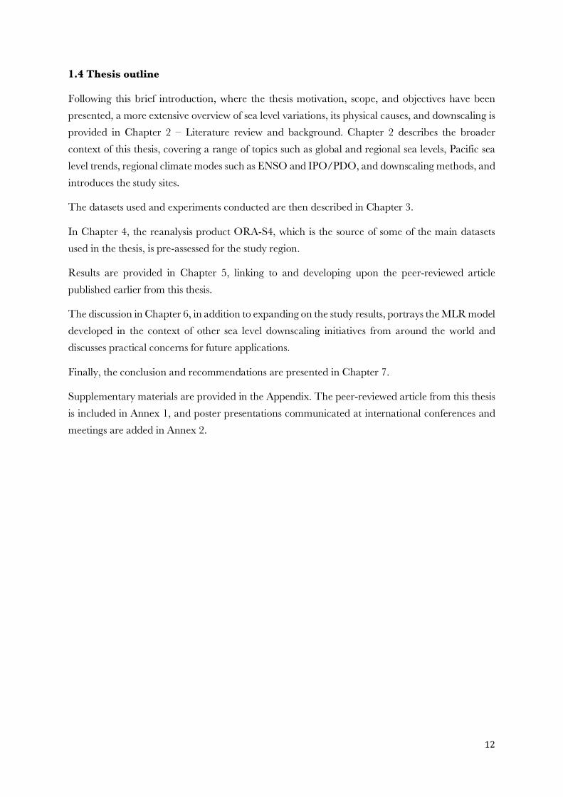
Figure 2.1: Global sea level over the last 2,500 years ........................................................... 16

Figure 2.2: Altimetry-based GMSL time series over the 1993-2017 period.. ...................... 17

Figure 2.3: GMSL budget time series over the 2005-2012 period ....................................... 19

Figure 2.4: Projections of global mean sea level rise over the 21st century relative to 1986–2005 for RCP2.6 and RCP8.5. ............................................................................................... 24

Figure 2.4: Global, regional, and local sea levels in context: sea level trends across the globe from satellite altimetry for the period 1993-2012 (map) ......................................................... 27

Figure 2.6: Schematic overview of local sea level processes. ................................................ 28

Figure 2.7: Tide gauge records available at the PSMSL database ....................................... 30

Figure 2.8: Sketch showing basic observational quantities and techniques associated with sea level measurement .................................................................................................................. 31

Figure 2.9: Sea level trends in the Pacific region over the 1993–2014 period from altimetry observations (GMSL trend included) ..................................................................................... 34

Figure 2.10: Schematic view of ocean and atmospheric conditions during the (a) neutral state, and anomalies during (b) El Niño and (c) La Niña. ....................................................... 36

Figure 2.11: SOI time series from 1880 to 2013. Negative SOI values correspond to El Niño conditions (blue) and positive SOI values to La Niña conditions (red). .................................. 37

Figure 2.12: Spatial signature of IPO based SST anomalies. .............................................. 38

Figure 2.13: IPO and PDO index time series from 1880 to 2016. ...................................... 39

Figure 2.14: The concept of spatial downscaling. ................................................................ 40

Figure 2.15: Map of the Fiji Islands, with study sites Suva and Lautoka marked. ............... 43

Figure 2.16: Map of New Caledonia, with study site Nouméa marked. .............................. 43

Figure 2.17: Schematic representation of inter-linked processes and components of sea level change. .................................................................................................................................... 46

Chapter 3 - Methodology and datasets

Figure 3.1: Illustration of the stepwise regression output (in Matlab) for the a given MLR experiment (undetrended, 1988-2014). . ................................................................................. 51

Figure 3.2: Location of the Suva tide gauge (a, b) and GPS station (a, b, c). ....................... 55

Figure 3.3: Location of the Lautoka tide gauge (a, b, c) and GPS station (a, d). .................. 55

Figure 3.4: Location of the Nouméa tide gauge (a, b) and GPS station (b), and the tide gauge inside the building. .................................................................................................................. 55

xiii

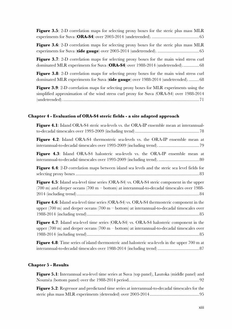
Figure 3.5: 2-D correlation maps for selecting proxy boxes for the steric plus mass MLR experiments for Suva (ORA-S4) over 2003-2014 (undetrended). .......................................... 65

Figure 3.6: 2-D correlation maps for selecting proxy boxes for the steric plus mass MLR experiments for Suva (tide gauge) over 2003-2014 (undetrended). ..................................... 65

Figure 3.7: 2-D correlation maps for selecting proxy boxes for the main wind stress curl dominated MLR experiments for Suva (ORA-S4) over 1988-2014 (undetrended). .............. 68

Figure 3.8: 2-D correlation maps for selecting proxy boxes for the main wind stress curl dominated MLR experiments for Suva (tide gauge) over 1988-2014 (undetrended). ......... 68

Figure 3.9: 2-D correlation maps for selecting proxy boxes for MLR experiments using the simplified approximation of the wind stress curl proxy for Suva (ORA-S4) over 1988-2014 (undetrended). ......................................................................................................................... 71

Chapter 4 - Evaluation of ORA-S4 steric fields - a site adapted approach

Figure 4.1: Island ORA-S4 steric sea-levels vs. the ORA-IP ensemble mean at interannual-to-decadal timescales over 1993-2009 (including trend) ......................................................... 78

Figure 4.2: Island ORA-S4 thermosteric sea-levels vs. the ORA-IP ensemble mean at interannual-to-decadal timescales over 1993-2009 (including trend). .................................... 79

Figure 4.3: Island ORA-S4 halosteric sea-levels vs. the ORA-IP ensemble mean at interannual-to-decadal timescales over 1993-2009 (including trend). .................................... 80

Figure 4.4: 2-D correlation maps between island sea levels and the steric sea level fields for selecting proxy boxes .............................................................................................................. 83

Figure 4.5: Island sea-level time series (ORA-S4) vs. ORA-S4 steric component in the upper (700 m) and deeper oceans (700 m – bottom) at interannual-to-decadal timescales over 1988-2014 (including trend) ............................................................................................................. 84

Figure 4.6: Island sea-level time series (ORA-S4) vs. ORA-S4 thermosteric component in the upper (700 m) and deeper oceans (700 m – bottom) at interannual-to-decadal timescales over 1988-2014 (including trend) .................................................................................................... 85

Figure 4.7: Island sea-level time series (ORA-S4) vs. ORA-S4 halosteric component in the upper (700 m) and deeper oceans (700 m – bottom) at interannual-to-decadal timescales over 1988-2014 (including trend) .................................................................................................... 85

Figure 4.8: Time series of island thermosteric and halosteric sea-levels in the upper 700 m at interannual-to-decadal timescales over 1988-2014 (including trend) ..................................... 87

Chapter 5 - Results

Figure 5.1: Interannual sea-level time series at Suva (top panel), Lautoka (middle panel) and Noumea (bottom panel) over the 1988-2014 period............................................................... 92

Figure 5.2: Regressor and predictand time series at interannual-to-decadal timescales for the steric plus mass MLR experiments (detrended) over 2003-2014 ............................................ 95

xiv

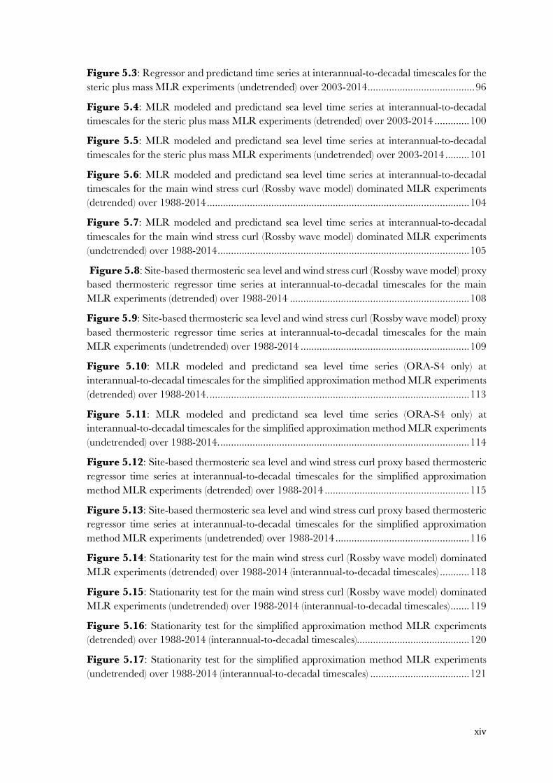
Figure 5.3: Regressor and predictand time series at interannual-to-decadal timescales for the steric plus mass MLR experiments (undetrended) over 2003-2014 ........................................ 96

Figure 5.4: MLR modeled and predictand sea level time series at interannual-to-decadal timescales for the steric plus mass MLR experiments (detrended) over 2003-2014 ............. 100

Figure 5.5: MLR modeled and predictand sea level time series at interannual-to-decadal timescales for the steric plus mass MLR experiments (undetrended) over 2003-2014 ......... 101

Figure 5.6: MLR modeled and predictand sea level time series at interannual-to-decadal timescales for the main wind stress curl (Rossby wave model) dominated MLR experiments (detrended) over 1988-2014 .................................................................................................. 104

Figure 5.7: MLR modeled and predictand sea level time series at interannual-to-decadal timescales for the main wind stress curl (Rossby wave model) dominated MLR experiments (undetrended) over 1988-2014 .............................................................................................. 105

Figure 5.8: Site-based thermosteric sea level and wind stress curl (Rossby wave model) proxy based thermosteric regressor time series at interannual-to-decadal timescales for the main MLR experiments (detrended) over 1988-2014 ................................................................... 108

Figure 5.9: Site-based thermosteric sea level and wind stress curl (Rossby wave model) proxy based thermosteric regressor time series at interannual-to-decadal timescales for the main MLR experiments (undetrended) over 1988-2014 ............................................................... 109

Figure 5.10: MLR modeled and predictand sea level time series (ORA-S4 only) at interannual-to-decadal timescales for the simplified approximation method MLR experiments (detrended) over 1988-2014. ................................................................................................. 113

Figure 5.11: MLR modeled and predictand sea level time series (ORA-S4 only) at interannual-to-decadal timescales for the simplified approximation method MLR experiments (undetrended) over 1988-2014. ............................................................................................. 114

Figure 5.12: Site-based thermosteric sea level and wind stress curl proxy based thermosteric regressor time series at interannual-to-decadal timescales for the simplified approximation method MLR experiments (detrended) over 1988-2014 ...................................................... 115

Figure 5.13: Site-based thermosteric sea level and wind stress curl proxy based thermosteric regressor time series at interannual-to-decadal timescales for the simplified approximation method MLR experiments (undetrended) over 1988-2014 .................................................. 116

Figure 5.14: Stationarity test for the main wind stress curl (Rossby wave model) dominated MLR experiments (detrended) over 1988-2014 (interannual-to-decadal timescales) ........... 118

Figure 5.15: Stationarity test for the main wind stress curl (Rossby wave model) dominated MLR experiments (undetrended) over 1988-2014 (interannual-to-decadal timescales) ....... 119

Figure 5.16: Stationarity test for the simplified approximation method MLR experiments (detrended) over 1988-2014 (interannual-to-decadal timescales).......................................... 120

Figure 5.17: Stationarity test for the simplified approximation method MLR experiments (undetrended) over 1988-2014 (interannual-to-decadal timescales) ..................................... 121

xv

Chapter 6 - Discussion

Figure 6.1: Island sea level for the study sites (ORA-S4) correlated with the basin-wide thermosteric sea level (a, c, e) and the Rossby wave modeled thermosteric change (b, d, f) at interannual-to-decadal time scales over 1988-2014 (undetrended). ..................................... 135

Figure .2: Time series of the Niño 3.4, IPO indices versus the dominant wind stress curl regressor for the main (Rossby wave model) MLR experiments over 1988-2014…………..141

xvi

List of Tables Chapter 2 – Literature review and background

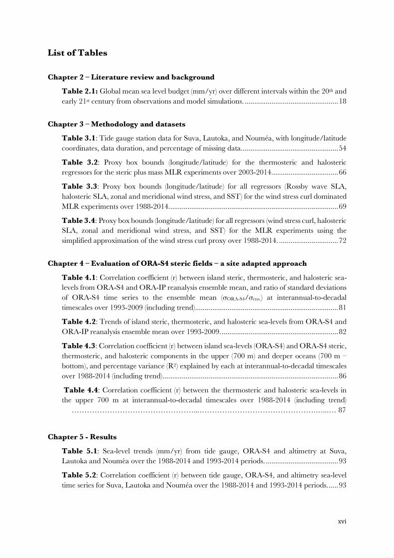
Table 2.1: Global mean sea level budget (mm/yr) over different intervals within the 20th and early 21st century from observations and model simulations. ................................................. 18

Chapter 3 – Methodology and datasets

Table 3.1: Tide gauge station data for Suva, Lautoka, and Nouméa, with longitude/latitude coordinates, data duration, and percentage of missing data. .................................................. 54

Table 3.2: Proxy box bounds (longitude/latitude) for the thermosteric and halosteric regressors for the steric plus mass MLR experiments over 2003-2014. .................................. 66

Table 3.3: Proxy box bounds (longitude/latitude) for all regressors (Rossby wave SLA, halosteric SLA, zonal and meridional wind stress, and SST) for the wind stress curl dominated MLR experiments over 1988-2014. ........................................................................................ 69

Table 3.4: Proxy box bounds (longitude/latitude) for all regressors (wind stress curl, halosteric SLA, zonal and meridional wind stress, and SST) for the MLR experiments using the simplified approximation of the wind stress curl proxy over 1988-2014. ............................... 72

Chapter 4 – Evaluation of ORA-S4 steric fields – a site adapted approach

Table 4.1: Correlation coefficient (r) between island steric, thermosteric, and halosteric sea-levels from ORA-S4 and ORA-IP reanalysis ensemble mean, and ratio of standard deviations of ORA-S4 time series to the ensemble mean (σORA-S4/σens.) at interannual-to-decadal timescales over 1993-2009 (including trend) ........................................................................... 81

Table 4.2: Trends of island steric, thermosteric, and halosteric sea-levels from ORA-S4 and ORA-IP reanalysis ensemble mean over 1993-2009. ............................................................. 82

Table 4.3: Correlation coefficient (r) between island sea-levels (ORA-S4) and ORA-S4 steric, thermosteric, and halosteric components in the upper (700 m) and deeper oceans (700 m – bottom), and percentage variance (R2) explained by each at interannual-to-decadal timescales over 1988-2014 (including trend) ............................................................................................ 86

Table 4.4: Correlation coefficient (r) between the thermosteric and halosteric sea-levels in the upper 700 m at interannual-to-decadal timescales over 1988-2014 (including trend) …………………………………………...……………………………………….…...… 87

Chapter 5 - Results

Table 5.1: Sea-level trends (mm/yr) from tide gauge, ORA-S4 and altimetry at Suva, Lautoka and Noumea over the 1988-2014 and 1993-2014 periods. ...................................... 93

Table 5.2: Correlation coefficient (r) between tide gauge, ORA-S4, and altimetry sea-level time series for Suva, Lautoka and Nouméa over the 1988-2014 and 1993-2014 periods. ..... 93

xvii

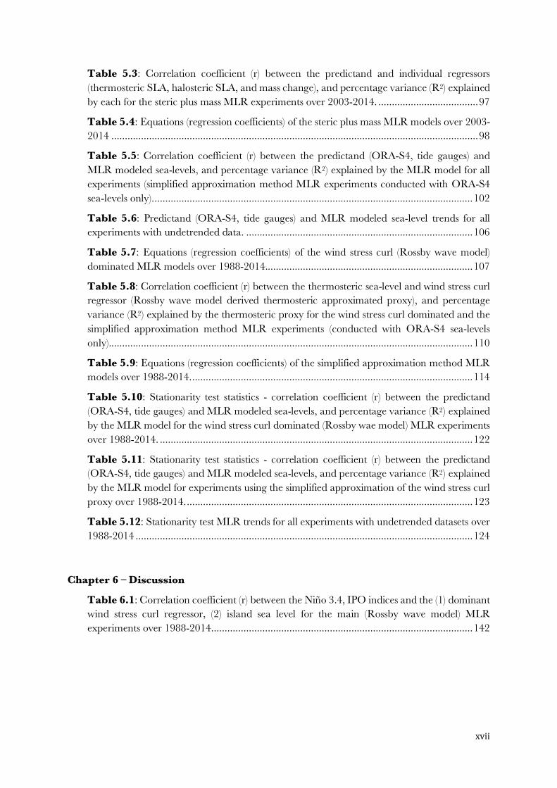
Table 5.3: Correlation coefficient (r) between the predictand and individual regressors (thermosteric SLA, halosteric SLA, and mass change), and percentage variance (R2) explained by each for the steric plus mass MLR experiments over 2003-2014. ..................................... 97

Table 5.4: Equations (regression coefficients) of the steric plus mass MLR models over 2003-2014 ........................................................................................................................................ 98

Table 5.5: Correlation coefficient (r) between the predictand (ORA-S4, tide gauges) and MLR modeled sea-levels, and percentage variance (R2) explained by the MLR model for all experiments (simplified approximation method MLR experiments conducted with ORA-S4 sea-levels only). ...................................................................................................................... 102

Table 5.6: Predictand (ORA-S4, tide gauges) and MLR modeled sea-level trends for all experiments with undetrended data. .................................................................................... 106

Table 5.7: Equations (regression coefficients) of the wind stress curl (Rossby wave model) dominated MLR models over 1988-2014............................................................................. 107

Table 5.8: Correlation coefficient (r) between the thermosteric sea-level and wind stress curl regressor (Rossby wave model derived thermosteric approximated proxy), and percentage variance (R2) explained by the thermosteric proxy for the wind stress curl dominated and the simplified approximation method MLR experiments (conducted with ORA-S4 sea-levels only)....................................................................................................................................... 110

Table 5.9: Equations (regression coefficients) of the simplified approximation method MLR models over 1988-2014. ........................................................................................................ 114

Table 5.10: Stationarity test statistics - correlation coefficient (r) between the predictand (ORA-S4, tide gauges) and MLR modeled sea-levels, and percentage variance (R2) explained by the MLR model for the wind stress curl dominated (Rossby wae model) MLR experiments over 1988-2014. .................................................................................................................... 122

Table 5.11: Stationarity test statistics - correlation coefficient (r) between the predictand (ORA-S4, tide gauges) and MLR modeled sea-levels, and percentage variance (R2) explained by the MLR model for experiments using the simplified approximation of the wind stress curl proxy over 1988-2014. .......................................................................................................... 123

Table 5.12: Stationarity test MLR trends for all experiments with undetrended datasets over 1988-2014 ............................................................................................................................. 124

Chapter 6 – Discussion

Table 6.1: Correlation coefficient (r) between the Niño 3.4, IPO indices and the (1) dominant wind stress curl regressor, (2) island sea level for the main (Rossby wave model) MLR experiments over 1988-2014 ................................................................................................. 142

xix

List of Abbreviations AMMA – African Monsoon Multidisciplinary Analysis

APB – Autonomous Pinniped Bathythermograph

AR5 – Assessment Report 5

CCA – Canonical Correlation Analysis

CTD – Conductivity, Temperature, Depth

CLARIS – Climate Change Assessment and Impact Studies

CMEMS – Copernicus Marine Environment Monitoring Service

CMIP5 – Coupled Model Intercomparison Project phase 5

CSIRO – Commonwealth Scientific and Industrial Research Organization

CORDEX – Coordinated Regional Climate Downscaling Experiment

CSR – Center for Space Research

DUACS – Data Unification and Altimeter Combination System

ECMWF – European Center for Medium-Range Weather Forecasts

ENSO – El Niño Southern Oscillation

EOF – Empirical Orthogonal Analysis

ERA – ECMWF Re-Analysis

GCM – General Circulation Model

GFZ – GeoForschungsZentrum

GMSL – Global Mean Sea Level

GNSS – Global Navigation Satellite Systems

GPS – Global Positioning System

GRACE – Gravity Recovery and Climate Experiment

GRGS – Groupe de Recherche de Geodesie Spatiale

IFS – Integrated Forecasting System

IPCC – Intergovernmental Panel on Climate Change

IPO – Interdecadal Pacific Oscillation

IRD – Institut de Recherche pour le Développement

ITCZ – Inter Tropical Convergence Zone

JPL – Jet Propulsion Laboratory

LEGOS – Laboratoire d’Études en Géophysique et Océanographie Spatiales

MEI – Multivariate ENSO Index

MEDRYS – MEDiterranean sea ReanalYsiS

MLR – Multiple Linear Regression

NARCCAP – North American Regional Climate Change Assessment Program

xx

NEMO – Nucleus for European Modeling of the Ocean

NEMOVAR – NEMO variational data assimilation

OCHA – United Nations Office for the Coordination of Humanitarian Affairs

OGCM – Ocean General Circulation Model

OMP – Observatoire Midi-Pyrénées

ORA-IP – Ocean Re-Analysis Intercomparison Project

ORA-S3 – Ocean Re-Analysis System 3

ORA-S4 – Ocean Re-Analysis System 4

PaCE-SD – Pacific Centre for Environment and Sustainable Development

PDO – Pacific Decadal Oscillation

PRUDENCE – Prediction of Regional scenarios and Uncertainties for Defining EuropeaN Climate change risks and Effects

PIRATA – Prediction and Research Moored Array in the Tropical Atlantic

PSMSL – Permanent Service for Mean Sea Level

RAMA – Research Moored Array for African-Asian-Australian Monsoon Analysis

RCP – Representative Concentration Pathway

REFMAR – Réseaux de référence des observations marégraphiques

RLR – Relative Local Reference

RMSE – Root Mean Square Error

SLA – Sea Level Anomaly

SLP – Sea Level Pressure

SOI – Southern Oscillation Index

SONEL – Système d'Observation du Niveau des Eaux Littorales

SPCZ – South Pacific Convergence Zone

SPM – Summary for Policy Makers

SSALTO – Segment Sol Multimission Altimetry and Orbitography

SSH – Sea Surface Height

SST – Sea Surface Temperature

STARDEX – STAtistical and Regional dynamical Downscaling of EXtremes for European regions

SVD – Singular Vector Decomposition

TAO – Tropical Atmosphere Ocean

ToE – Time of Emergence

TNI – Trans-Niño Index

TOPEX-Poseidon – Topography Experiment - Positioning, Ocean, Solid Earth, Ice Dynamics, Orbital Navigator

TRITON – Triangle Trans‐Ocean Buoy Network

xxi

TUG – Graz University of Technology

WMO – World Meteorological Organization

XBT – Expendable BathyThermograph

1

Introduction générale (en français)

Motivation

L’Océan Pacifique est le plus vaste océan du monde. Couvrant environ un vaste tiers de la surface de la Terre, l'océan Pacifique abrite de nombreux petits États insulaires en développement (PEID). L'océan est profondément enraciné dans les identités culturelles du Pacifique et joue un rôle important pour les moyens d’existence et les économies insulaires, sous-tendant des secteurs comme la pêche, le tourisme, la sécurité alimentaire, les transports et les loisirs. En englobant la plus grande zone océanique tropicale de la planète, le Pacifique est aussi le centre d'action de phénomènes climatiques majeurs comme El Niño Southern Oscillation et la Pacific Decadal Oscillation / Interdecadal Pacific Oscillation (PDO/IPO), et représente donc une zone d’intérêt pour la recherche sur le climat et l’océan. Au cours des dernières décennies, le Pacifique a enregistré les taux les plus élevés d'élévation du niveau de la mer dans le monde, ce qui a suscité un vif intérêt de la part de la communauté mondiale des chercheurs sur le climat et le niveau de la mer (e.g. Becker et al. 2012 ; Meyssignac et al. 2012 ; Han et al. 2014 ; Palanisamy et al. 2015a ; Marcos et al. 2017).

L'élévation du niveau de la mer est une conséquence directe du changement climatique en cours. Les tendances récentes du niveau de la mer présentent un aléa pour les zones côtières. Combiné à l’exposition des populations insulaires vivant en zone côtière et à la vulnérabilité de ces îles face au changement climatique et à la hausse du niveau de la mer (facteurs typiques tels que l'isolement géographique, le stress économique, les contraintes financières et le manque d'expertise humaine et technique), l’aléa associé à la hausse du niveau de la mer devient un risque majeur associé au changement climatique pour ces états insulaires du Pacifique (e.g. Barnett et Campbell 2010 ; Wong et al, 2014 ; Garschagen et al, 2016). Contrairement aux menaces à long-terme et/ou sporadiques liées au climat, l'élévation du niveau de la mer ne représente plus un risque pour le futur lointain ou un risque peu fréquent mais une réalité déjà présente dans de nombreuses zones côtières (Hallegatte et al. 2013 ; Wong et al. 2014 ; Neumann et al. 2015). Si les atolls coralliens de faible altitude sont certainement plus menacés que les îles volcaniques présentant des altitudes plus importantes, même ces dernières ont vu des communautés forcées de se déplacer en raison de l'intrusion d'eau salée dans les eaux de surface (sur terre) et les nappes phréatiques, de niveaux de la mer élévés pendant les périodes de vives-eaux des marées de périgée et des crues subites lors des événements extrêmes (Nurse et al. 2014 ; OCHA-ONU 2014 ; McNamara & Jacot Des Combes 2015 ; Albert et al. 2016).

A mesure que le réchauffement planétaire se poursuit, l'expansion thermique de l'eau de mer, la fonte des glaciers et la perte de masse des calottes glaciaires entraîneront une augmentation de l'élévation du niveau moyen de la mer (Jevrejeva et al. 2010 ; Church et al. 2011 ; Church et al. 2013) qui aggravera les impacts côtiers associés au niveau de la mer (inondations, intrusion saline, …). Compte tenu des trajectoires actuellement suivies pour les émissions de gaz à effet de serre, du réchauffement planétaire asssocié (Boyd et al. 2015 ; Höhne et al. 2017 ; Millar et al. 2017) et de la

2

mémoire longue des océans associées aux échelles de temps longues de la circulation profondes (Rhein et al. 2013), l'option la plus viable pour les îles menacées est une planification efficace des mesures d'adaptation et de réduction des risques. Pour que ces stratégies soient efficaces, il est essentiel de disposer d'informations solides à l'échelle locale.

De nos jours, les modèles numériques de climat sont les outils privilégiés pour comprendre le système climatique et sa prévisibilité à différentes échelles de temps et sous différentes perturbations. L'information provenant des modèles de climat sert à orienter les études de détection et d'attribution pour évaluer dans quelle mesure les changements observés sur la période instrumentale sont à attribuer au changement climatique (forçage anthropogénique) ou à la variabilité interne du système climatique. Les modèles de climat permettent également de produire des projections des conditions climatiques et océaniques sur les décennies et siècle(s) à venir. Ces informations sont essentielles au processus décisionnel des parties prenantes dans divers domaines tels que l'agriculture, la pêche, les infrastructures, l'urbanisme, la sécurité alimentaire et en eau, l'énergie, les transports, les assurances, l'adaptation, la prévention des risques, etc. Cependant, les incertitudes associées aux variables simulées par les modèles de climat deviennent plus importantes quand on s’intéresse à des échelles spatiales de plus en plus fine. Ceci est en partie du aux résolutions spatiales généralement grossières (~100 km) de ces modèles. Avec les résolutions utilisées dans les composantes océaniques des modèles de climat actuels, les petites îles ne sont pas résolues et sont perçues comme faisant partie de l'océan.

Cette thèse est motivée par le besoin urgent de disposer d'informations fiables sur le niveau de la mer à l'échelle locale, qui peuvent aider pour élaborer des mesures efficaces d'adaptation et de réduction des risques.

Le processus de génération d'information à haute résolution ou à l'échelle locale à partir de d’information à grande échelle est connu sous le nom de descente d’échelle (downscaling en anglais). Dans cette thèse, une technique de descente d'échelle statistique est utilisée pour reconstituer le niveau de la mer pour certains sites côtiers des îles du Pacifique Sud-Ouest - Suva et Lautoka dans les îles Fidji, et Nouméa en Nouvelle-Calédonie. Basée sur les connaissances existantes sur les processus responsables des variations régionales et locales du niveau de la mer dans le Pacifique tropical, l'approche utilise une combinaison de variables océaniques/atmosphériques comme prédicteurs pour formuler un modèle de régression linéaire multiple (multiple linear regression –MLR- en anglais) du niveau de la mer insulaire. Le niveau de la mer local ainsi modélisé à partir de variables à grande échelle présente une grande similitude (corrélation, variance expliquée) avec le niveau de la mer observé et peut être utilisé pour générer des projections des changements futurs du niveau de la mer à l'échelle locale et raffiner à l’échelles locale les modèles climatiques à grande échelle. L'approche peut également être adaptée à d'autres sites, en ajustant les combinaisons de variables fournissant l’information de grande échelle au besoin.

3

Les informations à l’échelle locale peuvent être utilisées par les parties prenantes et les décideurs pour affiner la planification de l'adaptation et de la réduction des risques. De cette façon, les résultats scientifiques sur la probabilité de changements futurs peuvent être appliqués jusqu'aux politiques et canaux et de mise en œuvre, devenant ainsi une partie du renforcement de la résilience dans le Pacifique.

Périmètre de l'étude

Cette thèse vise à construire un modèle statistique de descente d'échelle pour les variations interannuelles à inter-décennales du niveau de la mer pour trois sites côtiers situés sur des îles du Pacifique sud-ouest. Dans l'approche de descente d'échelle utilisée dans cette thèse, le niveau de la mer à un site donné (local) est fonction de régresseurs potentiels représentant des facteurs régionaux (à grande échelle) et locaux (à petite échelle) superposés à la moyenne globale (von Storch et al. 2000 ; Benestad et al. 2007). Le concept est appliqué aux sites d'étude sélectionnés à l'aide d'une régression linéaire multiple (MLR), un ensemble de variables océaniques et atmosphériques servant de régresseurs. Les variables explicatives permettent de représenter le niveau régional de la mer, qui s'avère dominant pour les trois sites étudiés ici, et les signatures locales. La moyenne globale est retirée du prédictand (niveau de la mer observé servant à calibrer le modèle MLR).

Dans la région du Pacifique, comme dans la plupart des régions du globe, les variations du niveau de la mer sont largement de nature stérique (i.e. liés à des changements de volume de l’océan induits par des changements de densité de l’eau de mer) avec une prédominance de la composante thermostérique (liées aux changements de densité induit par les changements de température). Aux échelles de temps interannuelles à décennales, les variations du niveau de la mer thermostérique sont en majeur partie générées par les variations de la tension du vent sur le bassin tropical (p. ex. Carton et al. 2005 ; Köhl et al. 2007 ; McGregor et al. 2012 ; Nidheesh et al. 2013 ; Timmermann et al. 2010). Les anomalies de rotationnel de tension de vent contrôlent la profondeur de la thermocline et le niveau de la mer stérique qui, en bonne approximation pour cette région, en est le miroir, en modulant le transport d’Ekman près de la surface, le pompage Ekman et la propagation vers l'ouest des ondes de Rossby. En tant que tel, les changements de la tension du vent représentent un facteur déterminant des tendances et des variations du niveau de la mer dans la région.

Dans le Pacifique Ouest, la propagation des ondes de Rossby explique la majeure partie de la variabilité du niveau de la mer (Fu et Qiu 2002 ; Qiu et Chen 2006 ; Lu et al. 2013) et un modèle linéaire en eau peu profonde à gravité réduite (modèle des ondes de Rossby) est utilisé pour modéliser la réponse du niveau de la mer thermostérique aux variations du forçage en vent. Le niveau de la mer fournit par le modèle d’ondes de Rossby s'avère être le principal régresseur dans le modèle de descente d’échelle MLR.

4

Une fonction de régression par étapes est d'abord utilisée pour isoler les régresseurs statistiquement significatifs, qui sont ensuite utilisés pour calibrer le modèle MLR. Les autres variables explicatives représentent les effets locaux : niveau de la mer halostérique, tension de vent et température de surface de l’océan pour, représenter respectivement, les flux d'eau douce, les surcotes liées au vent et les flux de chaleur de surface.

Comme la motivation sous-jacente à l'élaboration du modèle MLR est une application aux projections futures du niveau de la mer, la capacité du modèle à générer une information pertinente sur des périodes autres que celle sur laquelle il a été calibré est évaluée par un test de stationnarité. La performance du modèle sur des périodes autres que celles sur lesquelles il a été calibré est alors évaluée à la lumière du modèle MLR utilisé à plein potentiel.

L'analyse MLR est effectuée à la fois en utilisant des séries temporelles du niveau de la mer issues de l’estimation de l'état de l'océan (réanalyse ORA-S4) et de marégraphes in situ pour calibrer le modèle. Cependant, du fait que la réanalyse du niveau de la mer fait déjà partie de la méthodologie, la correction du mouvement vertical du sol (affaissement, soulèvement) affectant les enregistrements de marégraphes n'entre pas dans le cadre de cette thèse; les résultats sont plutôt pris en compte sur la base d'un tel mouvement lorsque des preuves sont disponibles (littérature, enregistrements, altimétrie).

L'étendue de la thèse va jusqu'au processus de calibration et du test de stationnarité du modèle MLR. Bien que l'application du modèle développé aux données CMIP5 a été plus que souhaitée, elle n'a pas été couverte en raison des contraintes de temps. Cependant, il est fortement prévu que les expériences MLR-CMIP5 soient poursuivies dans une étude de suivi.

Objectifs

Les objectifs de cette thèse sont les suivants :

i. Élaborer une régression linéaire multiple pour les variations interannelles à interdécennales du niveau de la mer pour trois sites insulaires en utilisant des variables océaniques/atmosphériques régionales et locales.

ii. Permettre une meilleure compréhension de l'importance relative des processus physiques pour les changements locaux du niveau de la mer sur les sites d'étude.

iii. Évaluer la performance globale du modèle MLR et identifier les sources d'erreur et la variance inexpliquée du modèle utilisé pour le niveau de la mer.

iv. Évaluer la stationnarité du modèle MLR développé par rapport aux projections futures du niveau de la mer.

5

Plan de thèse

Après cette brève introduction, où la motivation, la portée et les objectifs de la thèse sont présentés, un aperçu plus complet des variations du niveau de la mer, de ses causes physiques et de la réduction d'échelle est fourni au Chapitre 2 - Revue de la littérature et contexte. Le Chapitre 2 décrit le contexte plus large de cette thèse, couvrant un éventail de sujets tels que le niveau de la mer mondial et régional, les tendances du niveau de la mer du Pacifique, les modes climatiques régionaux tels que ENSO et IPO / PDO, et les méthodes de réduction d'échelle, et introduit les sites d'étude.

Les ensembles de données utilisés et les expériences menées sont ensuite décrits au Chapitre 3.

Au Chapitre 4, la méthode de sélection du produit de réanalyse, ORA-S4, qui est la source de certains des principaux ensembles de données utilisés dans la thèse, est pré-évaluée pour la région d'étude.

Les résultats sont fournis dans le Chapitre 5, reliant et développant sur l'article revu et publié durant la période de travail de cette thèse.

La discussion du Chapitre 6, en plus d'étendre les résultats de l'étude, décrit le modèle MLR développé dans le contexte d'autres initiatives de réduction d'échelle du niveau de la mer du monde entier et discute des préoccupations pratiques pour de futures applications.

Enfin, la conclusion et les recommandations sont présentées au Chapitre 7.

Des documents supplémentaires sont fournis en annexe. L'article revu et publié durant cette thèse est inclus dans l'annexe 1, et les contenus des affiches présentées lors des conférences et réunions internationales sont ajoutés dans l'annexe 2.

7

Chapter 1

Introduction 1.1 Motivation ................................................................................................ 9 1.2 Scope of the thesis .................................................................................... 10 1.3 Objectives ............................................................................................... 11 1.4 Thesis outline .......................................................................................... 12

9

1. Introduction

1.1 Motivation

The Pacific is the world’s largest ocean. Covering roughly a vast one third of the Earth’s surface area, the Pacific Ocean is home to numerous small island developing states (SIDS). The ocean is rooted deeply into Pacific cultural identities as well as island livelihoods and economies, underpinning sectors such as fisheries, tourism, food security, transportation and recreation. Encompassing the planet’s largest tropical ocean zone, the Pacific is also the origin and center of action of major climatic phenomenon like the El Niño Southern Oscillation (ENSO) and the Pacific Decadal Oscillation (PDO)/ Interdecadal Pacific Oscillation (IPO), and thus a hotspot for climate and ocean research. Over recent decades, the Pacific has recorded the highest rates of sea level rise across the globe, spurring keen interest from the climate and sea level research community worldwide (e.g. Becker et al. 2012; Meyssignac et al. 2012; Han et al. 2014; Palanisamy et al. 2015a; Marcos et al. 2017).

Sea level rise is a critical consequence of global warming and recent climate change. Recent sea level trends, combined with typical factors such as geographical isolation, economic stress, financial constraints, and lack of both human and technical expertise make the Pacific islands amongst the most vulnerable to ongoing climate and sea level changes (e.g. Barnett & Campbell 2010; Nicholls and Cazenave 2010; Wong et al., 2014; Garschagen et al. 2016;). Unlike long-term and/or sporadic climate-related threats, rising sea levels are no longer a distant or infrequent hazard but present reality in many coastal zones (Hallegatte et al. 2013; Wong et al. 2014; Neumann et al. 2015). While low-lying coral atolls are certainly more endangered than high rise volcanic islands, even the latter have had communities forced to relocate due to saltwater intrusion, perigean spring tides, and flash floods during extreme events (Hallegatte et al. 2013; Nurse et al. 2014; OCHA—United Nations 2014; McNamara & Jacot Des Combes 2015; Albert et al. 2016; Hinkel et al. 2019).

As global warming continues, thermal expansion of seawater, and melt of glaciers and ice sheets will lead to committed global mean sea level rise (e.g. Church et al. 2013; Levermann et al. 2013; Golledge et al. 2015; Mengel et al. 2018) exacerbating coastal impacts. Based on ongoing emission trajectories (Boyd et al. 2015; Höhne et al. 2017; Millar et al. 2017) and the slow thermal feedback of the ocean (Rhein et al. 2013), the more viable option on threatened islands is efficient adaptation. For such strategies to be effective, local scale information is essential (e.g. refined estimates of projected sea level changes, unambiguous probabilistic projections, best and worst-case scenarios of sea-level rise, etc. (e.g. Hinkel et al. 2019)).

In the present day, climate models serve as central tools for understanding the climate system and its predictability on various timescales and under different perturbations. Information from climate models is used to guide detection and attribution studies in the context of recent climate change and to generate projections of climate/ocean conditions on decadal to centennial timescales. This information is key in the decision-making process for policymakers across various domains such as

10

agriculture, fisheries, infrastructure, urban planning, food/water security, energy, transportation, insurance, adaptation, risk prevention, etc. Yet, while climate models are reliable for large-scale simulations, their skill is greatly reduced at small scales due to typically coarse spatial resolutions (~100 km for the ocean component). At this resolution, smaller islands are not well represented in the model, remaining unresolved and being perceived largely as part of the ocean. In addition, climate models do not represent all the physical processes that cause relative sea level changes at the coast.

Motivation for this thesis hence stems from the pressing need to have reliable sea level information on local scales, which can be used to develop efficient adaptation and risk minimization measures.

The process of obtaining high resolution, local scale information from large scale simulations is known as downscaling; this forms the basis of the present thesis. Here, a statistical downscaling technique is used to reconstruct island sea levels over the last decades at selected sites in the western South Pacific – Suva and Lautoka in the Fiji islands, and Nouméa in New Caledonia. Based on existing knowledge of regional and local sea level variations in the tropical Pacific, the approach uses a combination of oceanic/atmospheric variables as predictors to formulate a multiple linear regression model of island sea level. The modeled sea level bears high similarity to the observed/predictand and can be applied in generating projections for future sea level changes at the local scale. The approach can be easily adapted to other sites as well, adjusting the predictor combinations as appropriate.

Information at the local scale can be utilized by policymakers and stakeholders to refine adaptation and risk minimization practices on vulnerable islands, preventing loss to life, infrastructure and various other sectors in the longer future. In this way, scientific findings on the likelihood of future changes can be translated all the way to the policy and implementation channels, becoming part of resilience building in the Pacific.

1.2 Scope of the thesis

This thesis is based on constructing a statistical downscaling model for sea levels in the western South Pacific islands, focusing on interannual-to-decadal scale variability and trend. In this method, sea level at a given site is perceived as a function of regional (large scale) and local drivers (small scale), superimposed on the global mean (von Storch et al. 2000; Benestad et al. 2007). The concept is applied to the selected study sites using a multiple linear regression (MLR) approach, with a selection of oceanic and atmospheric variables serving as regressors.

In the Pacific region, as in most parts of the globe, sea level variations are largely steric (density related), with the thermosteric component (temperature related) predominating. On interannual-to-decadal timescales, thermosteric variations are driven by wind stress (e.g. Carton et al. 2005; Köhl et al. 2007; McGregor et al. 2012; Nidheesh et al. 2013; Timmermann et al. 2010). Wind

11

stress curl anomalies can control the thermocline depth and resultant sea levels in the tropical Pacific by modulating the near-surface Ekman transport, Ekman pumping, and westward propagating Rossby waves. As such, wind stress plays a critical role in determining sea levels trends and variations in the region. In the western Pacific, where the study sites are located, the wind forced propagation of Rossby waves is particularly relevant (Fu and Qiu 2002; Qiu and Chen 2006; Lu et al. 2013).

The MLR analysis begins with a preliminary set of experiments, where island sea levels are first expressed as a sum of steric and mass changes. A more dynamical approach is then undertaken, where wind stress curl is taken as a proxy for the thermosteric component. The MLR model uses regional wind stress curl as the dominant regressor and incorporates minor regressors representing local processes to simulate observed island sea levels.

As the underlying motive of developing the MLR model is to apply it to future projections of sea leve, a stationarity test comprised an integral part of the study. Here, the skill of the model over periods other than which it was calibrated over is assessed in light of the MLR model’s full potential.

The MLR analysis is performed using ocean reanalysis as well as tide gauge sea levels as predictands. However, especially since reanalysis sea levels are part of the analysis, correcting for vertical land motion (subsidence, uplift) affecting the tide gauge records is outside the scope of this thesis; the results rather are accounted for on the basis of such motion where evidence is available (literature, records, altimetry).

The extent of the thesis is till the calibration process and stationarity testing of the MLR model. While it was much aspired to apply the MLR model developed to CMIP5 data, it was not covered due to time constraints. However, it is intended that the MLR-CMIP5 experiments are pursed in a follow-up study.

1.3 Objectives

The objectives of this thesis are as follows:

i. To develop a multiple linear regression model for island sea level variations on interannual-to-decadal timescales using regional and local oceanic/atmospheric variables.

ii. To provide insights on the relative importance of physical processes to local sea level changes at the study sites.

iii. To evaluate the overall skill of the MLR model and identify sources of error and unexplained variance.

iv. To assess the stationarity of the MLR model developed in regards to future sea level projections.

12

1.4 Thesis outline

Following this brief introduction, where the thesis motivation, scope, and objectives have been presented, a more extensive overview of sea level variations, its physical causes, and downscaling is provided in Chapter 2 – Literature review and background. Chapter 2 describes the broader context of this thesis, covering a range of topics such as global and regional sea levels, Pacific sea level trends, regional climate modes such as ENSO and IPO/PDO, and downscaling methods, and introduces the study sites.

The datasets used and experiments conducted are then described in Chapter 3.

In Chapter 4, the reanalysis product ORA-S4, which is the source of some of the main datasets used in the thesis, is pre-assessed for the study region.

Results are provided in Chapter 5, linking to and developing upon the peer-reviewed article published earlier from this thesis.

The discussion in Chapter 6, in addition to expanding on the study results, portrays the MLR model developed in the context of other sea level downscaling initiatives from around the world and discusses practical concerns for future applications.

Finally, the conclusion and recommendations are presented in Chapter 7.

Supplementary materials are provided in the Appendix. The peer-reviewed article from this thesis is included in Annex 1, and poster presentations communicated at international conferences and meetings are added in Annex 2.

13

Chapter 2

Literature review and background 2.1 Sea level - Scientific context ................................................................... 15

2.1.1 Historical and contemporary sea level changes ......................................................... 15 2.1.2 Global mean sea level rise .......................................................................................... 18

2.1.2.1 Thermal expansion .......................................................................................... 19 2.1.2.2 Mass loss of glaciers and ice sheets .................................................................. 20 2.1.2.3 Terrestrial water storage .................................................................................. 22 2.1.2.4 Future projections ............................................................................................ 24

2.1.3 Regional sea levels ..................................................................................................... 25 2.1.4 Local sea levels ........................................................................................................... 27 2.1.5 Sea level observations – the instrumental era ............................................................ 30

2.1.5.1 Tide gauges ...................................................................................................... 30

2.1.5.2 Satellite altimetry ............................................................................................. 31 2.1.6 The case of the Pacific Ocean .................................................................................... 33

2.1.6.1 Pacific sea level trends ..................................................................................... 33 2.1.6.2 El Niño Southern Oscillation (ENSO) ............................................................ 35 2.1.6.3 Decadal variability – IPO and PDO ............................................................... 37

2.2 Downscaling - an introduction ............................................................... 39 2.2.1 Dynamical downscaling ............................................................................................. 40 2.2.2 Statistical downscaling ............................................................................................... 41 2.2.3 Downscaling method used - MLR ............................................................................. 42

2.3 Study sites .......................................................................................... 42

2.4 Synthesis and MLR Framework ............................................................. 44

15

2. Literature review and Background

This chapter provides a more detailed introduction to the main aspects of the thesis – sea level changes and downscaling.

There are various dimensions to sea level change, such as spatial and temporal variability, processes and components involved, natural and anthropogenic drivers, and so on. Under the sea level section, this chapter covers historical to contemporary changes, variations on global/regional/local scales, sea level observations, recent trends in the Pacific Ocean, and the major climate modes in this region (ENSO and IPO/PDO).

The section following explains the concept of downscaling and why it is needed. It also describes the two main approaches to downscaling, dynamical and statistical. The downscaling method used in this thesis is also briefly presented.

The study sites are introduced towards the end, and the chapter concludes with a synthesis of the information provided here in the framework of statistical downscaling of island sea levels.

2.1 Sea level – scientific context

2.1.1 Historical and contemporary sea level changes

Sea level changes have occurred throughout Earth’s history, covering a wide range of spatial and temporal scales. They provide a glimpse into the tectonic and climate history of the planet, reflecting the ocean’s response to various changes over millennia (e.g. Kominz 2001).

Paleo data in the form of coastal/shoreline records, emergent shoreline deposits, marine/salt marsh sediments, oxygen-18 isotopes in fossils and ice cores, dating of corals, to name a few, have allowed the investigation of sea levels back into centuries to millennia (Douglas et al. 2001; Kemp et al. 2011; Masson-Delmotte et al. 2013). Information has been retrieved from archaeological evidence as well, with the example of ancient fish tanks in the Mediterranean basin making it possible to estimate local sea levels during the Roman era, 2000 years ago (Lambeck et al. 2004). These records reflect both local and global conditions (Masson-Delmotte et al. 2013).

The largest global scale sea level changes, in orders of 100–200 m, are estimated to have occurred about 100 million years ago. These were related mainly to tectonic processes, such as large scale changes in the shape of the oceans basins associated with the spreading of the sea-floor and the expansion of mid-ocean ranges (Haq and Schutter 2008, Müller et al. 2008; Miller et al. 2011). Later, as the Antarctic ice-sheet formed (~34 million years ago), the GMSL receded by about 50 m (Douglas et al. 2001).

In the more recent past, about 3 million years ago, the cooling of the Earth has induced glacial/interglacial cycles controlled by changes in incoming insolation due to variations in the

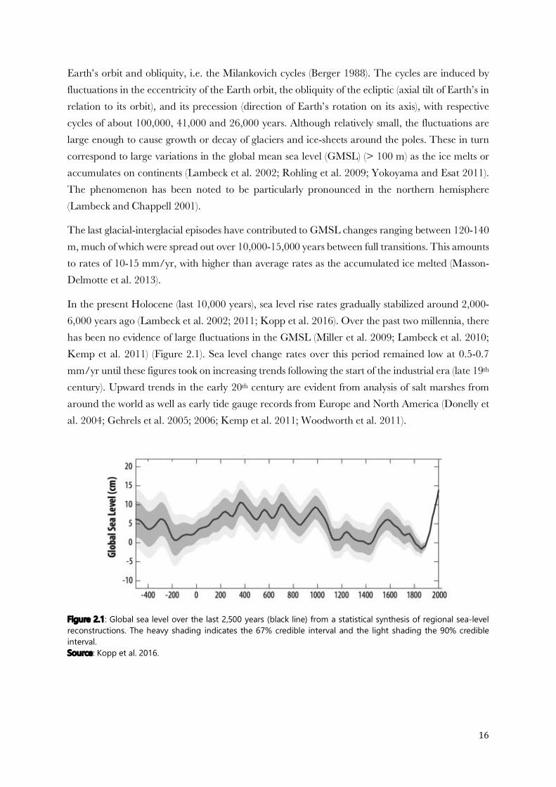
16

Earth’s orbit and obliquity, i.e. the Milankovich cycles (Berger 1988). The cycles are induced by fluctuations in the eccentricity of the Earth orbit, the obliquity of the ecliptic (axial tilt of Earth’s in relation to its orbit), and its precession (direction of Earth’s rotation on its axis), with respective cycles of about 100,000, 41,000 and 26,000 years. Although relatively small, the fluctuations are large enough to cause growth or decay of glaciers and ice-sheets around the poles. These in turn correspond to large variations in the global mean sea level (GMSL) (> 100 m) as the ice melts or accumulates on continents (Lambeck et al. 2002; Rohling et al. 2009; Yokoyama and Esat 2011). The phenomenon has been noted to be particularly pronounced in the northern hemisphere (Lambeck and Chappell 2001).

The last glacial-interglacial episodes have contributed to GMSL changes ranging between 120-140 m, much of which were spread out over 10,000-15,000 years between full transitions. This amounts to rates of 10-15 mm/yr, with higher than average rates as the accumulated ice melted (Masson-Delmotte et al. 2013).

In the present Holocene (last 10,000 years), sea level rise rates gradually stabilized around 2,000-6,000 years ago (Lambeck et al. 2002; 2011; Kopp et al. 2016). Over the past two millennia, there has been no evidence of large fluctuations in the GMSL (Miller et al. 2009; Lambeck et al. 2010; Kemp et al. 2011) (Figure 2.1). Sea level change rates over this period remained low at 0.5-0.7 mm/yr until these figures took on increasing trends following the start of the industrial era (late 19th century). Upward trends in the early 20th century are evident from analysis of salt marshes from around the world as well as early tide gauge records from Europe and North America (Donelly et al. 2004; Gehrels et al. 2005; 2006; Kemp et al. 2011; Woodworth et al. 2011).

Figure 2.1: Global sea level over the last 2,500 years (black line) from a statistical synthesis of regional sea-level reconstructions. The heavy shading indicates the 67% credible interval and the light shading the 90% credible interval. Source: Kopp et al. 2016.

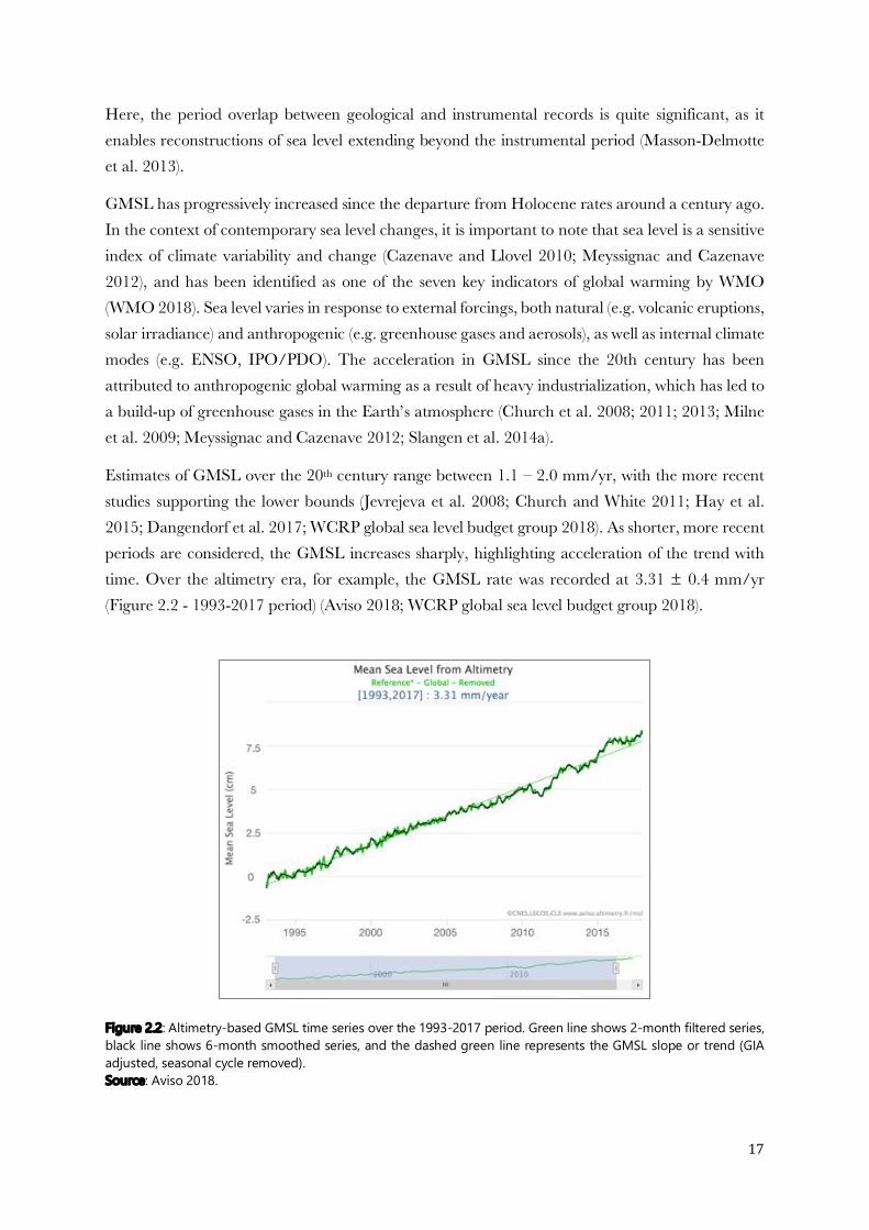
17

Here, the period overlap between geological and instrumental records is quite significant, as it enables reconstructions of sea level extending beyond the instrumental period (Masson-Delmotte et al. 2013).

GMSL has progressively increased since the departure from Holocene rates around a century ago. In the context of contemporary sea level changes, it is important to note that sea level is a sensitive index of climate variability and change (Cazenave and Llovel 2010; Meyssignac and Cazenave 2012), and has been identified as one of the seven key indicators of global warming by WMO (WMO 2018). Sea level varies in response to external forcings, both natural (e.g. volcanic eruptions, solar irradiance) and anthropogenic (e.g. greenhouse gases and aerosols), as well as internal climate modes (e.g. ENSO, IPO/PDO). The acceleration in GMSL since the 20th century has been attributed to anthropogenic global warming as a result of heavy industrialization, which has led to a build-up of greenhouse gases in the Earth’s atmosphere (Church et al. 2008; 2011; 2013; Milne et al. 2009; Meyssignac and Cazenave 2012; Slangen et al. 2014a).

Estimates of GMSL over the 20th century range between 1.1 – 2.0 mm/yr, with the more recent studies supporting the lower bounds (Jevrejeva et al. 2008; Church and White 2011; Hay et al. 2015; Dangendorf et al. 2017; WCRP global sea level budget group 2018). As shorter, more recent periods are considered, the GMSL increases sharply, highlighting acceleration of the trend with time. Over the altimetry era, for example, the GMSL rate was recorded at 3.31 ± 0.4 mm/yr (Figure 2.2 - 1993-2017 period) (Aviso 2018; WCRP global sea level budget group 2018).

Figure 2.2: Altimetry-based GMSL time series over the 1993-2017 period. Green line shows 2-month filtered series, black line shows 6-month smoothed series, and the dashed green line represents the GMSL slope or trend (GIA adjusted, seasonal cycle removed). Source: Aviso 2018.

18

It is important to note that while geological records indicate much larger rates of historical sea level change compared to present rates, the former occurred under special circumstances such as glacial-interglacial transitions or major tectonic activity. As such, both geological and instrumental records indicate that the current GMSL rates are anomalous when compared to estimates over the last 2,000 years (Masson-Delmotte et al. 2013).

2.1.2 Global mean sea level rise

The two main causes of contemporary GMSL changes are the thermal expansion of seawater as it warms and mass addition to the ocean from melting of glaciers and ice sheets under warmer air temperatures. Additionally, GMSL is affected by water exchange from terrestrial reservoirs (e.g. water bodies, snow packs) (Cazenave and Llovel 2010; Meyssignac and Cazenave 2012; Church et al. 2013).

The different contributions to the rising GMSL trend over different periods are summarized in Table 2.1, and modeled and observed values compared. In addition, the observed GMSL time series, together with thermal expansion and freshwater mass addition components are illustrated in Figure 2.3 (2005-2012). The contributing factors are discussed in detail afterwards (Sections 2.1.2.1-2.1.2.3).

Table 2.1: Global mean sea level budget (mm/yr) over different intervals within the 20th and early 21st century from observations and model simulations. Uncertainty ranges are 5-9%. Source: Church et al. 2013 (IPCC AR5).

1151

Sea Level Change Chapter 13

13

heat uptake (Levitus et al., 2001). The models including natural forcing are closer to observations, though with a tendency to underestimate the trend by about 10% (Sections 9.4.2.2 and 10.4.1).

Gregory (2010) and Gregory et al. (2013a) proposed that AOGCMs underestimate ocean heat uptake in their historical simulations because their control experiments usually omit volcanic forcing, so the imposition of historical volcanic forcing on the simulated climate system represents a time mean negative forcing relative to the con-trol climate. The apparent long persistence of the simulated oceanic cooling following the 1883 eruption of Krakatau (Delworth et al., 2005; Gleckler et al., 2006a, 2006b; Gregory et al., 2006) is a consequence of this bias, which also causes a model-dependent underestimate of up to 0.2 mm yr–1 of thermal expansion on average during the 20th century (Gregory et al., 2013a, 2013b). This implies that CMIP5 results may be similarly underestimated, depending on the details of the indi-vidual model control runs. Church et al. (2013) proposed a correction of 0.1 mm yr–1 to the model mean rate, which we apply in the sea level budget in Table 13.1 and Figure 13.7. The corrected CMIP5 model mean rate for 1971–2010 is close to the central observational estimate; the model mean rate for 1993–2010 exceeds the central observational estimate but they are not statistically different given the uncertainties (Table 13.1 and Figure 13.4a). This correction is not made to projec-tions of thermal expansion because it is very small compared with the projected increase in the rate (Section 13.5.1).

In view of the improvement in observational estimates of thermal expansion, the good agreement of historical model results with obser-vational estimates, and their consistency with understanding of the

energy budget and RF of the climate system (Box 13.1), we have high confidence in the projections of thermal expansion using AOGCMs.

13.3.2 Glaciers

13.3.2.1 Observed

‘Glaciers’ are defined here as all land-ice masses, including those peripheral to (but not including) the Greenland and Antarctic ice sheets. The term ‘glaciers and ice caps’ was applied to this category in the AR4. Changes in aggregate glacier volume have conventional-ly been determined by various methods of repeat mapping of surface elevation to detect elevation (and thus volume) change. Mass changes are determined by compilation and upscaling of limited direct observa-tions of surface mass balance (SMB). Since 2003, gravity observations from Gravity Recovery and Climate Experiment (GRACE) satellites have been used to detect mass change of the world’s glaciers.

The combined records indicate that a net decline of global glacier volume began in the 19th century, before significant anthropogenic RF had started, and was probably the result of warming associated with the termination of the Little Ice Age (Crowley, 2000; Gregory et al., 2006, 2013b). Global rates of glacier volume loss did not increase significantly during much of the 20th century (Figure 4.12). In part this may have been because of an enhanced rate of loss due to unforced high-latitude variability early in the century, while anthropogenic warming was still comparatively small (Section 13.3.2.2). It is likely that anthropogenic forcing played a statistically significant role in acceleration of global glacier losses in the latter decades of the 20th

Table 13.1 | Global mean sea level budget (mm yr–1) over different time intervals from observations and from model-based contributions. Uncertainties are 5 to 95%. The Atmo-sphere–Ocean General Circulation Model (AOGCM) historical integrations end in 2005; projections for RCP4.5 are used for 2006–2010. The modelled thermal expansion and glacier contributions are computed from the CMIP5 results, using the model of Marzeion et al. (2012a) for glaciers. The land water contribution is due to anthropogenic intervention only, not including climate-related fluctuations.

Notes:a Data for all glaciers extend to 2009, not 2010.b This contribution is not included in the total because glaciers in Greenland are included in the observational assessment of the Greenland ice sheet.c Observed GMSL rise – modelled thermal expansion – modelled glaciers – observed land water storage.

Source 1901–1990 1971–2010 1993–2010Observed contributions to global mean sea level (GMSL) rise

Thermal expansion – 0.8 [0.5 to 1.1] 1.1 [0.8 to 1.4]

Glaciers except in Greenland and Antarcticaa 0.54 [0.47 to 0.61] 0.62 [0.25 to 0.99] 0.76 [0.39 to 1.13]

Glaciers in Greenlanda 0.15 [0.10 to 0.19] 0.06 [0.03 to 0.09] 0.10 [0.07 to 0.13]b

Greenland ice sheet – – 0.33 [0.25 to 0.41]

Antarctic ice sheet – – 0.27 [0.16 to 0.38]

Land water storage –0.11 [–0.16 to –0.06] 0.12 [0.03 to 0.22] 0.38 [0.26 to 0.49]

Total of contributions – – 2.8 [2.3 to 3.4]

Observed GMSL rise 1.5 [1.3 to 1.7] 2.0 [1.7 to 2.3] 3.2 [2.8 to 3.6]

Modelled contributions to GMSL rise

Thermal expansion 0.37 [0.06 to 0.67] 0.96 [0.51 to 1.41] 1.49 [0.97 to 2.02]

Glaciers except in Greenland and Antarctica 0.63 [0.37 to 0.89] 0.62 [0.41 to 0.84] 0.78 [0.43 to 1.13]

Glaciers in Greenland 0.07 [–0.02 to 0.16] 0.10 [0.05 to 0.15] 0.14 [0.06 to 0.23]

Total including land water storage 1.0 [0.5 to 1.4] 1.8 [1.3 to 2.3] 2.8 [2.1 to 3.5]

Residualc 0.5 [0.1 to 1.0] 0.2 [–0.4 to 0.8] 0.4 [–0.4 to 1.2]

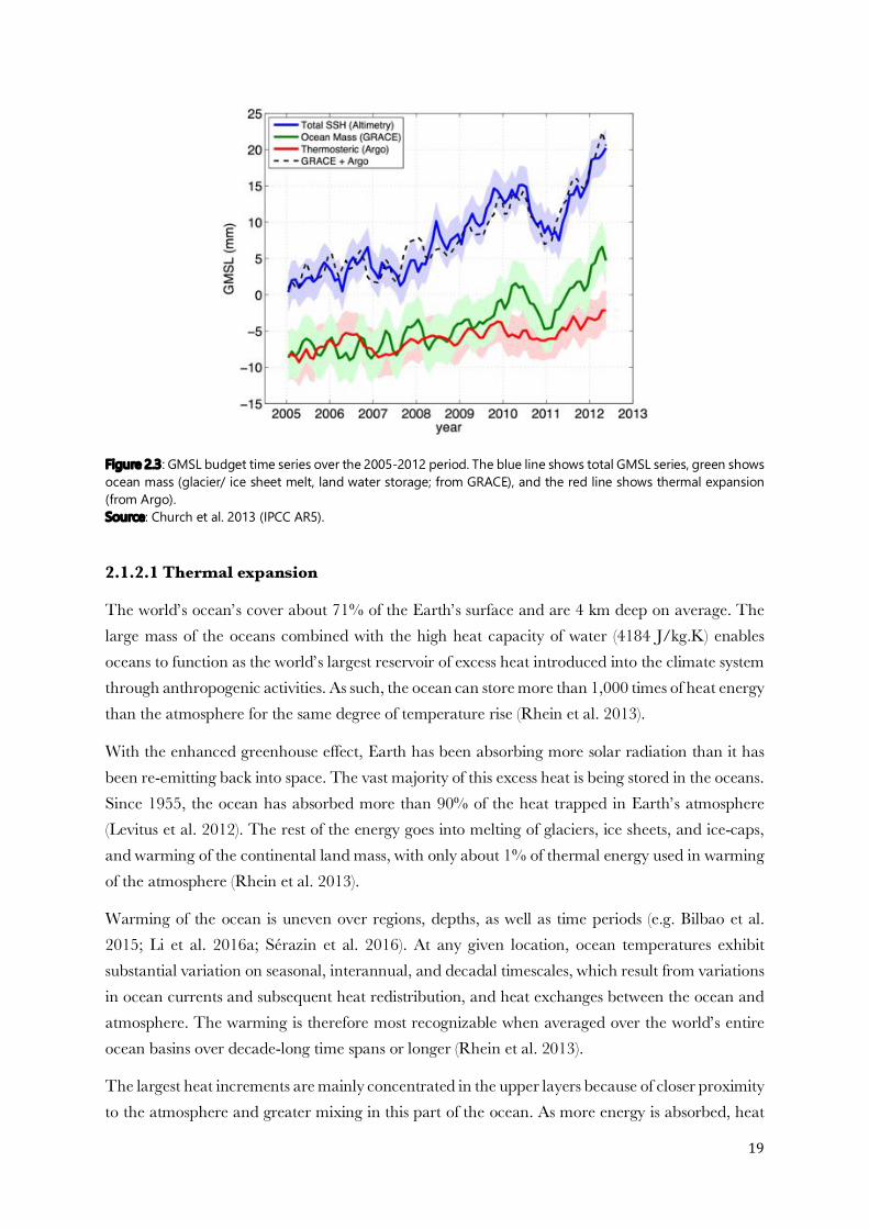
19

Figure 2.3: GMSL budget time series over the 2005-2012 period. The blue line shows total GMSL series, green shows ocean mass (glacier/ ice sheet melt, land water storage; from GRACE), and the red line shows thermal expansion (from Argo). Source: Church et al. 2013 (IPCC AR5).

2.1.2.1 Thermal expansion

The world’s ocean’s cover about 71% of the Earth’s surface and are 4 km deep on average. The large mass of the oceans combined with the high heat capacity of water (4184 J/kg.K) enables oceans to function as the world’s largest reservoir of excess heat introduced into the climate system through anthropogenic activities. As such, the ocean can store more than 1,000 times of heat energy than the atmosphere for the same degree of temperature rise (Rhein et al. 2013).

With the enhanced greenhouse effect, Earth has been absorbing more solar radiation than it has been re-emitting back into space. The vast majority of this excess heat is being stored in the oceans. Since 1955, the ocean has absorbed more than 90% of the heat trapped in Earth’s atmosphere (Levitus et al. 2012). The rest of the energy goes into melting of glaciers, ice sheets, and ice-caps, and warming of the continental land mass, with only about 1% of thermal energy used in warming of the atmosphere (Rhein et al. 2013).

Warming of the ocean is uneven over regions, depths, as well as time periods (e.g. Bilbao et al. 2015; Li et al. 2016a; Sérazin et al. 2016). At any given location, ocean temperatures exhibit substantial variation on seasonal, interannual, and decadal timescales, which result from variations in ocean currents and subsequent heat redistribution, and heat exchanges between the ocean and atmosphere. The warming is therefore most recognizable when averaged over the world’s entire ocean basins over decade-long time spans or longer (Rhein et al. 2013).

The largest heat increments are mainly concentrated in the upper layers because of closer proximity to the atmosphere and greater mixing in this part of the ocean. As more energy is absorbed, heat

20

penetrates deeper into the ocean via circulation pathways and mixing, and even direct sinking in the polar zones (Schlesinger and Jiang 1988; Huang et al. 2003; Zika et al. 2015; Liu et al. 2016).

Over the 1971-2010 period, global mean temperatures in the upper 75 m of the ocean have increased by 0.11 ºC (0.09-0.13 ºC) per decade. This value generally decreases with depth, reducing to less than 0.02 ºC per decade at 500 m. About 64% of the heat absorbed by the ocean over this period has been confined to the upper 700 m of the ocean, while 30% is distributed in the deeper layers (Rhein et al. 2013). In terms of sea level, whereby the global mean rise due to thermal expansion is almost proportional to the increase in ocean heat content, this translates to ~ 40% of the observed global mean trend (Table 2.1) (Church et al. 2013).

The large heat capacity of the ocean combined with the long timescales of thermohaline circulation (slow thermal feedback) gives it substantially high thermal inertia. Hence, if greenhouse emissions were ceased today, while reductions in the Earth’s rising surface temperatures would start becoming noticeable within roughly a decade, warming of the deep oceans would continue for centuries to millennia. Thus, sea levels would continue to rise as well (Collins et al. 2013; Levermann et al. 2013; Rhein et al. 2013; Mengel et al. 2018).

2.1.2.2 Mass loss of glaciers and ice sheets

Glaciers, in the context of freshwater mass addition to oceans, cover all perennial surface land ice outside the Antarctic and Greenland ice sheets1. They form from snow accumulation over several years, which transforms to firn and finally to ice. Glaciers are sensitive indicators of climate, quickly adjusting their size to temperature and precipitation changes (Church et al. 2013; Vaughan et al. 2013).

The Greenland and Antarctic ice sheets make up the largest component of the cryosphere, containing more than 99% of the freshwater present on Earth. Melted completely, Greenland and West Antactica2 would raise sea level by approximately 7 and 3 m respectively (Church et al. 2013; Vaughan et al. 2013). Thus, even a small loss in mass from the ice sheets can cause marked sea level rise and exacerbate existing threats.

Together, the added mass from melt of glaciers and ice sheets has accounted for about 45% of the GMSL trend over the 1993-2010 period (Church et al. 2013), making it the largest contributor during this time. Further details on the two components are discussed below:

1 IPCC AR5 classification 2 Vulnerable portion of the Antarctic to melting

21

Glaciers

Glaciers make up a very small fraction of the total ice surface (~4%). Yet, glacier melt comprised approximately 30% of the total GMSL rise over the 20th century, making it the second largest contributor after thermal expansion. Even though the Greenland and Antarctic ice sheets are magnitudes larger, glacier response to warming is quite rapid, accounting for the relatively larger observed melt (Steffen et al. 2010; Meyssignac and Cazenave 2012; Church et al. 2013; Vaughan et al. 2013).

The critical aspect between glaciers and GMSL is the mass balance, which is the sum of all accumulation and ablation (melting, sublimation) processes. A negative mass balance evidences a retreating glacier and therefore added melt to the GMSL.

Total glacier coverage was only roughly known until 2009-2010. The glacier inventory is drawn up with repeated measurements of glacier length, area, volume, or mass using a combination of techniques such in situ measurements, remote sensing, reconstructions, etc. Nonetheless, datasets still have large observational uncertainties (Cogley 2009; Radić and Hock 2010; Vaughan et al. 2013).

Glaciers contributed 0.62 mm/yr to the observed GMSL trend over the period 1971-2010. Over 1993-2010, the contribution increased to 0.76 mm/yr, which was about 24% of the GMSL trend (Table 2.1) (Church et al. 2013).

Glacier loss projections for the 21st century range between median values of 0.10 and 0.16 m of sea level rise by 2100, depending on the RCP scenario3 used for Earth’s future radiative forcing. As for the 20th century, glaciers are likely to remain the second largest contributor to GMSL rise over the 21st century. Furthermore, since glaciers can take several decades to adjust to rapid climate changes, they will continue losing mass from current warming even if temperatures stabilize in the near future (Meier et al. 2007; Church et al. 2013; Vaughan et al. 2013).

Ice Sheets

While not much information was available on ice sheets before the 1990s, development of remote sensing techniques (e.g. air-borne, radar, laser altimetry, gravimetry) have greatly improved observations of the Greenland and Antarctic ice sheets. The three main techniques applied are the mass budget method, repeat altimetry, and gravimetry (e.g. Fettweis 2007; Jacob et al. 2012; Lenaerts et al. 2012; Helm et al. 2014). Substantial mass loss has been observed in the Greenland and West Antarctic ice sheets, with accelerated rates in the recent years (Vaughan et al. 2013; Forsberg et al. 2017).

3 IPCC “Representative Concentration Pathways” (RCPs) for different possible emission scenarios in future (Moss et al. 2010; Cubasch et al. 2013)

22

It is important to note that the two ice sheets, pertaining to marked differences in aspects such as extent, ice characteristics, continental elevation, effective circulation patterns, and processes at work, produce dissimilar melt responses to warming. Here, clear distinction between the West and East Antarctic sheets must be drawn as well, where the latter, together with the Antarctic Peninsula, is the zone of Antarctic melt while the former has recorded increases in snow accumulation. Furthermore, paleo data evidence collapse of the West Antarctic ice sheet during the last interglacial, emphasizing its vulnerability, whereas the East Antarctic is believed to be more stable in comparison (Vaughan et al. 2013; Feldmann and Levermann 2015; Gulick et al. 2017; Hillenbrand et al. 2017). Net change in the Antarctic ice sheet had been uncertain in previous estimates, however, recent advancements indicate that enhanced outflow currently exceeds any increase in accumulation (i.e. sea level rise) (Church et al. 2013).

Between 1993 and 2010, the sum of mass contributions of Greenland and Antarctica to sea level was 0.60 mm/yr (~ 19% of GMSL trend). Over the 2005-2010 period, this contribution increased to 1.04 mm/yr, a high ~ 38% of the GMSL trend, evidencing recent acceleration in melt rates. Over the two periods 1993-2010 and 2005-2010, the contribution of Greenland (Antarctica) was 0.33 (0.27) mm/yr and 0.63 (0.41) mm/yr respectively (Church et al. 2013; Vaughan et al, 2013).

Projections for sea level rise from the sum of mass contributions from the two ice sheets by the end of the 21st century range between median values of 0.11 and 0.16 m across the RCP scenarios (Church et al. 2013). However, the estimates do not include collapse of marine ice sheets4 such as the West Antarctic, which would substantially increase the projected range of sea level rise. Once initiated, such a collapse would continue independently of climate and unfold over centuries for West Antarctica and parts of East Antarctica (Church et al. 2013; Collins et al. 2013).

Greenland, on the other hand, has no large-scale instabilities as such. However, potentially irreversible nonlinear mass loss is possible if ongoing ablation rates surpass a certain threshold. Sea level rise from such a response would become substantial over the 22nd century and beyond (Church et al. 2013; Collins et al. 2013).

2.1.2.3 Terrestrial water storage

Aside from governing contributions from thermal expansion and sum of mass additions from glacier/ice sheet melt, GMSL rises and falls with corresponding water loss and gain from continents. Terrestrial water occurs as snow packs, surface water, and subsurface water.

4 Marine ice sheet instability refers to the susceptibility of marine-based ice sheets (bedrock submerged below sea level) to rapidly lose ice mass from the interior to downward sloping ice shelves, where warming waters instigate melt and disintegration. The cycle continues as the grounding line i.e. the boundary separating the ice sheet and the floating ice shelf gradually moves up the ice sheet slope, destabilizing it over time. Major marine ice sheets/glaciers are West Antarctic, and the Totten and Cook glaciers in the East Antarctic.

23

Surface water includes rivers, lakes, reservoirs, and wetlands. Subsurface includes soil moisture, aquifers/groundwater, and the vadose zone (Milly et al. 2010; Syed et al. 2010; Church et al. 2013).

Terrestrial water storage changes are driven by both natural and anthropogenic factors. These factors include climate variations, direct human intervention in the water cycle, and human modifications to the physical land surface (Milly et al. 2003; 2010).

Climate affects terrestrial storage on seasonal to much longer timescales. The largest terrestrial-source seasonal variations in GMSL are from snow packs at high latitudes/altitudes (accumulation and melt annual cycle) (Milly et al. 2003; 2010; Chambers et al. 2004; Biancamaria et al. 2011). On internannual-to-decadal timescales, the largest source of variation in terrestrial storage is ENSO. During El Niño events, GMSL temporarily rises as precipitation over the ocean increases and land precipitation in the tropics decreases (e.g. 1997-98 event). The opposite occurs during La Niñas, where GMSL lowers with increased precipitation over Australia, northern South America, and southeast Asia (Nerem et al. 2010; Syed et al. 2010; Llovel et al. 2011; Boening et al. 2012).

Direct human intervention constitutes the largest changes in terrestrial storage, with leading yet opposite contributions from water impoundment in reservoirs and groundwater extraction (Gornitz 2001; Huntington 2008; Lettenmaier and Milly 2009; Wada et al. 2017). From roughly the second half of the 20th century, reservoirs have collectively counterbalanced sea level rise that would have occurred otherwise. Groundwater extraction reduces terrestrial water storage, with most of the extracted water eventually ending up in the ocean via runoff, evaporation, and precipitation. Other human activities affecting the terrestrial water budget, including modification of the physical environment, include irrigation, wetland drainage, urbanization, and deforestation (Sahagian 2000; Gornitz 2001; Chao et al. 2008; Milly et al. 2010; Konikow 2011; Wada et al. 2017).

Over time, no significant long-term trends have been found in climate-related variations in terrestrial water storage (Milly et al. 2003; 2010; Ngo-Duc et al. 2005; Biancamaria et al. 2011). Anthropogenic activities - reservoir impoundment and groundwater extraction in particular, however have contributed significantly to sea level change. Although contribution from reservoir impoundment surpassed groundwater extraction over the majority of the 20th century, present extraction rates exceed impoundment, resulting in net sea level rise.

As such, terrestrial storage changes contributed a negative 0.11 m/yr (i.e. sea level fall) to the GMSL rate over most of the 20th century (1901-1990). Nearing the end of century, terrestrial storage began adding to sea level rise, with a rate of 0.12 mm/yr reported over the period 1971-2010 (6% GMSL trend). More recently, for the period 1993-2010, the contribution escalated to 0.38 mm/yr, doubling to ~12% of the GMSL trend (Church et al. 2013).

Projections for the net contribution of terrestrial water storage to GMSL rise by the end of the 21st century span a broad range between -10 to 90 mm, owing to limited available information (Katsman et al. 2008; Church et al. 2013).

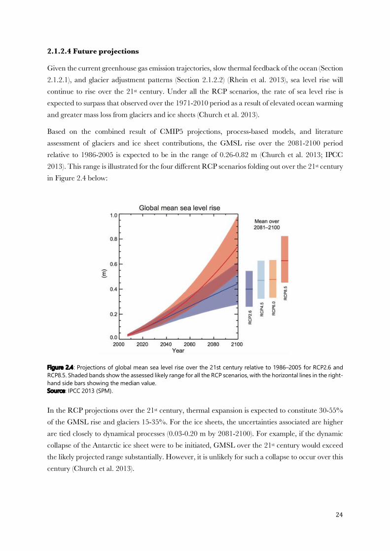
24

2.1.2.4 Future projections

Given the current greenhouse gas emission trajectories, slow thermal feedback of the ocean (Section 2.1.2.1), and glacier adjustment patterns (Section 2.1.2.2) (Rhein et al. 2013), sea level rise will continue to rise over the 21st century. Under all the RCP scenarios, the rate of sea level rise is expected to surpass that observed over the 1971-2010 period as a result of elevated ocean warming and greater mass loss from glaciers and ice sheets (Church et al. 2013).

Based on the combined result of CMIP5 projections, process-based models, and literature assessment of glaciers and ice sheet contributions, the GMSL rise over the 2081-2100 period relative to 1986-2005 is expected to be in the range of 0.26-0.82 m (Church et al. 2013; IPCC 2013). This range is illustrated for the four different RCP scenarios folding out over the 21st century in Figure 2.4 below:

Figure 2.4: Projections of global mean sea level rise over the 21st century relative to 1986–2005 for RCP2.6 and RCP8.5. Shaded bands show the assessed likely range for all the RCP scenarios, with the horizontal lines in the right-hand side bars showing the median value. Source: IPCC 2013 (SPM). In the RCP projections over the 21st century, thermal expansion is expected to constitute 30-55% of the GMSL rise and glaciers 15-35%. For the ice sheets, the uncertainties associated are higher are tied closely to dynamical processes (0.03-0.20 m by 2081-2100). For example, if the dynamic collapse of the Antarctic ice sheet were to be initiated, GMSL over the 21st century would exceed the likely projected range substantially. However, it is unlikely for such a collapse to occur over this century (Church et al. 2013).

25

It is projected that sea level rise will be experienced in over 95% of the ocean areas by the end of the 21st century. Sea level rise will not be uniform, with about 70% of the coastlines projected to experience a rise within 20% of the global mean (Church et al. 2013; IPCC 2013).

2.1.3 Regional sea levels

Sea level varies markedly on regional scales. While the global mean is the critical indicator of sea level change, regional sea levels provide a practical perspective and illustrate the heterogeneity in sea levels across the globe. The advent of satellite altimetry has enabled mapping of regional sea level variability in a way that was not possible before, allowing for high precisions and almost complete global coverage (Cazenave and Llovel 2010; Rhein et al. 2013).

Regional sea level variations are governed largely by sea or basin-specific dynamical forcings (i.e. driven by wind and ocean circulation) and manifest as changes in the steric component (e.g. Church et al. 2013; Stammer et al. 2013). This steric change arises essentially from redistribution of heat and freshwater, and to a small extent from surface fluxes (Lu et al. 2013; Stammer et al. 2013; Meyssignac et al. 2017). Resultant steric changes are mainly thermosteric in nature, although halosteric effects are significant in some regions and tend to compensate the thermosteric (e.g. tropical South Pacific, North Atlantic, East Indian) (Antonov et al. 2002; Köhl 2014; Forget and Ponte 2015; Llovel and Lee 2015). A large part of dynamical sea level variability is directly associated with natural internal climate modes, such as ENSO and IPO/PDO in the case of the Pacific Ocean (Section 2.1.6) (Lombard et al. 2005; Levitus et al. 2009; Becker et al. 2012; Meyssignac et al. 2012; Zhang & Church 2012; Stammer et al. 2013). As wind and ocean circulation patterns in a region undergo variations with phase transitions of the dominant climate modes, sea level adjusts in response.

Ocean numerical models have demonstrated thermosteric changes in the tropics to be driven by wind stress and related circulation patterns (Carton et al. 2005; Köhl et al. 2007; Timmermann et al., 2010; McGregor et al. 2012; Nidheesh et al., 2013). Here, wind stress can control the thermocline depth and resultant sea levels by modulating the near-surface Ekman transport, Ekman pumping, and consequent oceanic Rossby waves (Lu et al. 2013; Stammer et al. 2013). As such, wind stress plays a critical role in determining and/or reproducing regional sea levels.

There are exceptions at high latitudes and in shallow shelf seas, however, where regional variability is dominated by the mass change component and the steric plays a minor role (GIA, gravitational changes discussed later in this section) (Volkov and Landerer 2013; Purkey et al. 2014).

Aside from dynamical variability, the other components of regional sea level can be classified as static (Stammer et al. 2013; Kopp et al. 2015). This form of variability refers to the isostatic response of the ocean as it balances to changes in the Earth’s surface load. Examples include the inverted barometer effect (atmospheric loading), glacial isostatic adjustment (GIA), gravitational changes, as

26

well as changes in terrestrial water storage (Cazenave and Llovel 2010; Stammer et al. 2013). Apart from the inverted barometer effect, static processes are mainly non-climatic.

The inverted barometer effect simply represents the inverse relation between sea level and atmospheric pressure, whereby each 1 mbar increase in local sea level pressure suppresses sea level by 1 cm (Wunsch and Stammer 1997). On interannual timescales and longer, associated regional sea level variability ranges between less than 1 cm in the tropics to 2-3 cm at high latitudes (Ponte 2006; Piecuch and Ponte 2015). Compared to the rest of the static sea level drivers, the inverted barometer effect is a relatively minor contributor to sea level variability (Stammer and Hüttemann 2008; Carson et al. 2016).

GIA describes the gradual, ongoing adaptation of the solid Earth to the last deglaciation, which entails changes in the geoid and gravitational deformation of the ocean basins and sea surface (Peltier 2004; Peltier et al. 2015). Averaged across the oceans, GIA has been estimated to lower sea level by ~1 mm/yr (Chambers et al. 2010; Tamisea and Mitrovica 2011; Stammer et al. 2013).

Gravitational changes further arise with ice mass loss from ice sheets and glaciers. The vast mass of the ice sheets exerts slight gravitational pull on the surrounding waters, making sea level a bit higher around the edges. As ice mass is lost with higher melt rates, gravitational pull exerted formerly weakens, lowering sea level around. Thus, while the added mass to oceans raises sea levels further away, sea levels close to the ice sheet fall (Mitrovica et al. 2009; Bamber and Riva 2010; Tamisea and Mitrovica 2011).

The overall changes in mass distribution from such processes further affect Earth’s inertia tensor and rotation, producing an additional sea level response (Mitrovica et al. 2001).

Regional sea level variations arise from changes in terrestrial water storage also, driven mainly by natural climate variability modes. Oscillation patterns such as ENSO and IPO/PDO, for example, induce regional sea level variations via associated changes in precipitation patterns as their phases change (see Section 2.1.2.3) (Nerem et al. 2010; Syed et al. 2010; Llovel et al. 2011; Boening et al. 2012. Note how in this case the range of variable changes involved in climate mode transitions overlap with both dynamical and static sea level changes. Human induced changes in terrestrial water storage, particularly from groundwater extraction and irrigation, produce more localized changes and affect relative sea levels (covered in Section 2.1.4) (e.g. Gornitz 2001; Wada et al. 2017).

To summarize, regional sea levels are governed by several dynamical and static process acting on various timescales. While regional sea level variability is largely steric (dynamic origins), the importance of mass and gravitational changes (static origins) cannot be overlooked, especially at low latitudes.

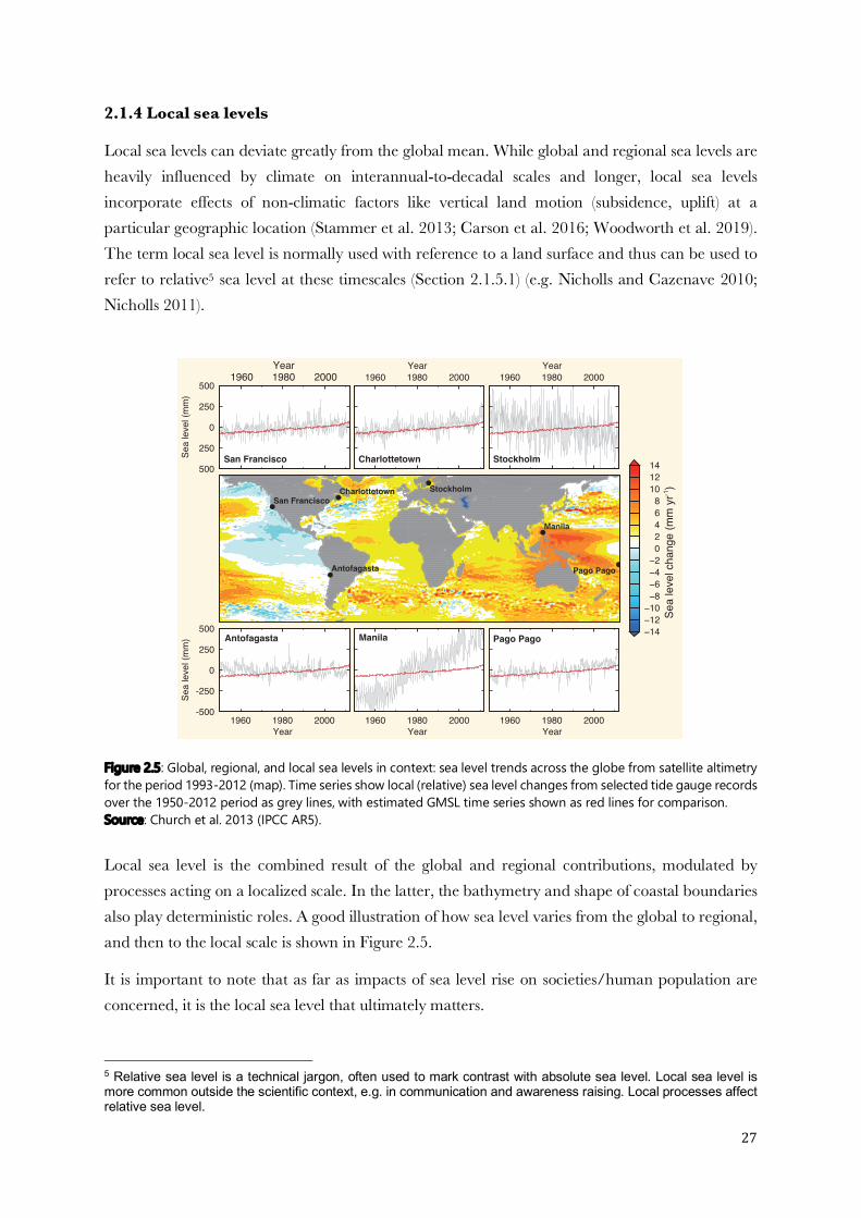
27

2.1.4 Local sea levels

Local sea levels can deviate greatly from the global mean. While global and regional sea levels are heavily influenced by climate on interannual-to-decadal scales and longer, local sea levels incorporate effects of non-climatic factors like vertical land motion (subsidence, uplift) at a particular geographic location (Stammer et al. 2013; Carson et al. 2016; Woodworth et al. 2019). The term local sea level is normally used with reference to a land surface and thus can be used to refer to relative5 sea level at these timescales (Section 2.1.5.1) (e.g. Nicholls and Cazenave 2010; Nicholls 2011).

Figure 2.5: Global, regional, and local sea levels in context: sea level trends across the globe from satellite altimetry for the period 1993-2012 (map). Time series show local (relative) sea level changes from selected tide gauge records over the 1950-2012 period as grey lines, with estimated GMSL time series shown as red lines for comparison. Source: Church et al. 2013 (IPCC AR5). Local sea level is the combined result of the global and regional contributions, modulated by processes acting on a localized scale. In the latter, the bathymetry and shape of coastal boundaries also play deterministic roles. A good illustration of how sea level varies from the global to regional, and then to the local scale is shown in Figure 2.5.

It is important to note that as far as impacts of sea level rise on societies/human population are concerned, it is the local sea level that ultimately matters.

5 Relative sea level is a technical jargon, often used to mark contrast with absolute sea level. Local sea level is more common outside the scientific context, e.g. in communication and awareness raising. Local processes affect relative sea level.

1148

Chapter 13 Sea Level Change

13

Frequently Asked Questions FAQ 13.1 | Why Does Local Sea Level Change Differ from the Global Average?

Shifting surface winds, the expansion of warming ocean water, and the addition of melting ice can alter ocean cur-rents which, in turn, lead to changes in sea level that vary from place to place. Past and present variations in the distribution of land ice affect the shape and gravitational field of the Earth, which also cause regional fluctuations in sea level. Additional variations in sea level are caused by the influence of more localized processes such as sedi-ment compaction and tectonics.

Along any coast, vertical motion of either the sea or land surface can cause changes in sea level relative to the land (known as relative sea level). For example, a local change can be caused by an increase in sea surface height, or by a decrease in land height. Over relatively short time spans (hours to years), the influence of tides, storms and climatic variability—such as El Niño—dominates sea level variations. Earthquakes and landslides can also have an effect by causing changes in land height and, sometimes, tsunamis. Over longer time spans (decades to centuries), the influ-ence of climate change—with consequent changes in volume of ocean water and land ice—is the main contributor to sea level change in most regions. Over these longer time scales, various processes may also cause vertical motion of the land surface, which can also result in substantial changes in relative sea level.

Since the late 20th century, satellite measurements of the height of the ocean surface relative to the center of the Earth (known as geocentric sea level) show differing rates of geocentric sea level change around the world (see FAQ 13.1, Figure 1). For example, in the western Pacific Ocean, rates were about three times greater than the global mean value of about 3 mm per year from 1993 to 2012. In contrast, those in the eastern Pacific Ocean are lower than the global mean value, with much of the west coast of the Americas experiencing a fall in sea surface height over the same period. (continued on next page)

Pago PagoManilaAntofagasta

San Francisco Charlottetown Stockholm

Antofagasta

Manila

Pago Pago

−14−12−10−8−6−4−2

02468

101214

Sea

level

chan

ge (m

m yr

-1)

500

250

0

250

500

Sea

level

(mm)

1960 1980 2000Year

San Francisco

1960 1980 2000Year

Charlottetown

1960 1980 2000Year

Stockholm

-500

-250

0

250

500

Sea

level

(mm)

1960 1980 2000Year

1960 1980 2000Year

1960 1980 2000Year

FAQ13.1, Figure 1 | Map of rates of change in sea surface height (geocentric sea level) for the period 1993–2012 from satellite altimetry. Also shown are relative sea level changes (grey lines) from selected tide gauge stations for the period 1950–2012. For comparison, an estimate of global mean sea level change is also shown (red lines) with each tide gauge time series. The relatively large, short-term oscillations in local sea level (grey lines) are due to the natural climate variability described in the main text. For example, the large, regular deviations at Pago Pago are associated with the El Niño-Southern Oscillation.

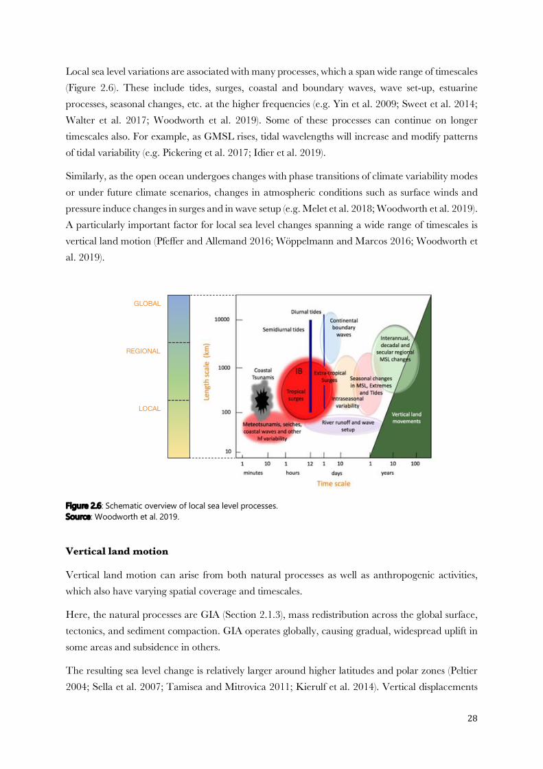
28

Local sea level variations are associated with many processes, which a span wide range of timescales (Figure 2.6). These include tides, surges, coastal and boundary waves, wave set-up, estuarine processes, seasonal changes, etc. at the higher frequencies (e.g. Yin et al. 2009; Sweet et al. 2014; Walter et al. 2017; Woodworth et al. 2019). Some of these processes can continue on longer timescales also. For example, as GMSL rises, tidal wavelengths will increase and modify patterns of tidal variability (e.g. Pickering et al. 2017; Idier et al. 2019).

Similarly, as the open ocean undergoes changes with phase transitions of climate variability modes or under future climate scenarios, changes in atmospheric conditions such as surface winds and pressure induce changes in surges and in wave setup (e.g. Melet et al. 2018; Woodworth et al. 2019). A particularly important factor for local sea level changes spanning a wide range of timescales is vertical land motion (Pfeffer and Allemand 2016; Woppelmann and Marcos 2016; Woodworth et al. 2019).

Figure 2.6: Schematic overview of local sea level processes. Source: Woodworth et al. 2019.

Vertical land motion

Vertical land motion can arise from both natural processes as well as anthropogenic activities, which also have varying spatial coverage and timescales.

Here, the natural processes are GIA (Section 2.1.3), mass redistribution across the global surface, tectonics, and sediment compaction. GIA operates globally, causing gradual, widespread uplift in some areas and subsidence in others.

The resulting sea level change is relatively larger around higher latitudes and polar zones (Peltier 2004; Sella et al. 2007; Tamisea and Mitrovica 2011; Kierulf et al. 2014). Vertical displacements

LOCAL

REGIONAL

GLOBAL

29

also result from the redistribution of water mass across the Earth’s surface, plus related loading of the solid Earth from present day ice melt (Section 2.1.2.2) and changes in terrestrial water storage (Section 2.1.2.3) (Santamaría-Gomez and Memin 2015; Frederikse et al. 2019). On more localized scales, tectonic processes may cause either gradual uplift or subsidence, although more abrupt changes are associated with volcanic eruptions and earthquakes (e.g. Aoki and Scholtz 2009; Ballu et al. 2011; Piccini and Iandelli 2011). In low-lying coastal zones and deltas, natural sediment compaction can occur as particles lose water from interstitial spaces pressured by overlying weight or as they rearrange, resulting in land subsidence (e.g. Tornqvist et al. 2008; Brown and Nicholls 2015). Of course, while land uplift has a counteracting effect on local sea level rise, subsidence exacerbates the problem, intensifying the risks associated.

Anthropogenic activities, on the other hand, include intensive groundwater pumping, mining, hydrocarbon extraction, water impoundment6, and settling of landfill in highly populated coastal and delta zones. These can notably exacerbate or even dominate the rate of natural sediment compaction, resulting in land subsidence (e.g. Mazzotti et al. 2009, Fiedler and Conrad 2010; Kolker et al. 2011; Ingebritsen and Galloway 2014; Brown and Nicholls 2015; Veit and Conrad 2016). Unlike for most natural processes (except volcanoes and earthquakes), anthropogenic induced vertical motion is rapid and highly localized. In areas of high exploitation, ensuing subsidence may surpass the global or regional mean, becoming the leading contributor to relative sea level rise. Some examples of such cases include the Adriatic Sea (Fenoglio-Marc et al. 2012), Gulf of Mexico (Douglas 2005), Manila (Raucoules et al. 2013), Jakarta (Abidin et al. 2001), and Bangkok (Saramul and Ezer 2014).

While the global, regional, and local components all add up over time to produce sea level change at any given site, the relative contribution of each varies greatly from one coastline to another. Thus, while the global or regional mean may dominate at some places, vertical land motion may dominate at others (e.g. Ballu et al. 2011; Raucoules et al. 2013; Brown and Nicholls 2015). As such, is it crucial to incorporate estimates of vertical land motion where possible when analyzing local sea level trends (tide gauge records). This enables the observed changes to be correctly attributed to the causes, without mistaking land subsidence for sea level rise or climate change (e.g. Ballu et al. 2011).

6 While water impoundment in reservoirs overall reduces the GMSL trend (Section 2.1.2.3), the water load depresses the land surface underneath and elevates the geoid, leading to a higher relative sea level (Fiedler and Conrad 2010).

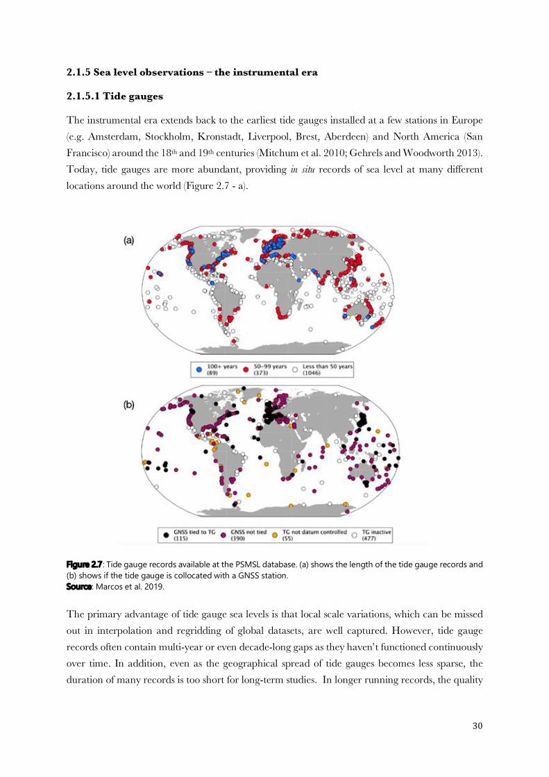
30

2.1.5 Sea level observations – the instrumental era

2.1.5.1 Tide gauges

The instrumental era extends back to the earliest tide gauges installed at a few stations in Europe (e.g. Amsterdam, Stockholm, Kronstadt, Liverpool, Brest, Aberdeen) and North America (San Francisco) around the 18th and 19th centuries (Mitchum et al. 2010; Gehrels and Woodworth 2013). Today, tide gauges are more abundant, providing in situ records of sea level at many different locations around the world (Figure 2.7 - a).

Figure 2.7: Tide gauge records available at the PSMSL database. (a) shows the length of the tide gauge records and (b) shows if the tide gauge is collocated with a GNSS station. Source: Marcos et al. 2019. The primary advantage of tide gauge sea levels is that local scale variations, which can be missed out in interpolation and regridding of global datasets, are well captured. However, tide gauge records often contain multi-year or even decade-long gaps as they haven’t functioned continuously over time. In addition, even as the geographical spread of tide gauges becomes less sparse, the duration of many records is too short for long-term studies. In longer running records, the quality

31

of the dataset is often a concern. Hence, it is difficult to estimate reliable historical mean sea level variations from tide gauge records alone (e.g. Meyssignac and Cazenave 2012).

Tide gauges measure relative sea level, i.e. sea level with respect to the Earth’s crust where they are grounded. As a result, any vertical land motion, either natural or human-induced (Section 2.1.4), is incorporated into the sea level observation as well. Depending on the site, vertical land motion can match or even surpass the climate-related signal in sea level (Section 2.1.4 and references therein). Thus, precise estimates of vertical land motion are crucial to separate the land and ocean contributions to sea level change in tide gauge records, and make correct attributions.

Currently, the global positioning system (GPS), which is part of the Global Navigation Satellite Systems (GNSS), provides the most accurate way to quantify vertical land motion around tide

gauges. The main limitations, however, are that continuous GPS observations are still short in duration (less than 20 years in most places), and stations may not always be close to the tide gauge (Figure 2.7 -b) (Woppelmann et al. 2007; Santamaría-Gomez et al. 2012; 2014; Woppelmann and Marcos 2016; Marcos et al. 2019). It is generally assumed that GPS records of vertical land motion, despite the short duration, are representative of long-term trends (Meyssignac and Cazenave 2012).

Figure 2.8: Sketch showing basic observational quantities and techniques associated with sea level measurement. Source: Marcos et al. 2019.

2.1.5.2 Satellite altimetry

The advent of satellite altimetry has provided the sea level community with an unprecedented opportunity to study sea level variations across the globe. While tide gauges had earlier suggested

Surveys in Geophysics

1 3

2 Coastal Sea-Level Observations: Tide Gauges and Satellite Altimetry

Tide gauges are the primary source of coastal sea-level observations, providing point-wise measurements of relative mean sea level and extreme sea levels (Intergovernmental Oceanographic Commission 1985). Initially designed for maritime navigation purposes, some of the oldest tide gauge records date back to the eighteenth century (e.g., Woodworth and Blackman 2002; Wöppelmann et al. 2006). These earliest sea-level observations were measured with tide poles and registered the time and height of tidal high and low waters (e.g., Woodworth and Blackman 2002). Since the nineteenth century, stilling well floating gauges have become the most used technology and still represent the majority of the avail-able records (Pugh and Woodworth 2014), while originally recording sea-level oscillations in tidal charts, during the twentieth century they have been upgraded to provide digital storage and transmission of data. New tidal stations tend to use radar gauges that measure the distance above the sea surface by analysing the time-of-flight of an electromagnetic reflected pulse. This type of gauge is nowadays preferred since it is relatively cheap, easy to install and able to measure at high frequencies with the required accuracy and long-term stability (Martín Míguez et al. 2008).

Tide gauges measure relative sea level with respect to the land upon which they are grounded (Fig. 1). Thus, to ensure continuity of the sea-level record, tide gauge measure-ments must refer to a properly defined datum, generally a fixed point on land referred to as tide gauge benchmark. Continuity can be achieved by systematically measuring the stabil-ity of the tide gauge benchmark through high-precision levelling with nearby land points

Fig. 1 Sketch showing basic observational quantities and techniques associated with sea-level measurement discussed in this article

32

spatial variations in sea level, the first maps of regional sea levels were produced with altimetric observations (Fu and Cazenave 2001; Meyssignac and Cazenave 2012; Church et al. 2013).

The first nearly global observations of sea level made by satellite altimetry were in the 1970s and 1980s. These measurements were still highly uncertain and short in duration (Rhein et al. 2013). High precision altimetry began later in 1992 with the launch of the TOPEX/Poseidon satellite and has since continued with various missions (e.g. Fu and Cazenave 2001; Ablain et al. 2017).

Satellite altimeters derive sea level measurements by transmitting microwave radiation via radar towards the sea surface. Part of the radar signal is reflected back to the satellite, and the time taken for the signal to return is used to compute the height above the instantaneous sea surface. Sea surface height is then calculated from the difference between the satellite’s distance from Earth’s center of mass (derived from precise orbitography) and its altitude above the sea surface (derived from the radar altimeter measurement) (Figure 2.8). The measurement is corrected for various factors, including adjustments for instrument, orbit, ionosphere, dry/wet troposphere, dynamic atmosphere correction, tides, sea state bias, and the mean sea surface (Pujol et al. 2016; CMEMS 2018).

Unlike tide gauges, which measure the combined effect of the ocean volume change and vertical land motion, altimetry provides absolute sea level, which is with respect to the Earth’s center of mass. Satellites measure sea level with respect to the geoid – a reference ellipsoid that matches the mean shape of the Earth. Altimetry sea level thus remains unaffected by vertical land motion effects. However, a small correction is still made to adjust for the GIA in order to account for the gradually changing location of the ocean bottom with respect to the satellite’s frame of reference. This correction value depends on the area that the satellite covers, and is approximately 0.3 mm/yr (Peltier 2004). Ocean reanalyses

In addition to in situ and altimetric observations, sea levels can be accessed from ocean reanalyses. Ocean reanalyses are historical reconstructions of the ocean climate, which combine a data assimilation system with an ocean general circulation model (OGCM) to produce a consistent and coherent dataset. The assimilated data consist of in situ and remote sensing observations, and the ocean model is forced with atmospheric surface fluxes. By combining observations with an ocean model, reanalyses datasets can potentially provide more accurate ocean information than observation-only or model-only based estimates. As such, they are invaluable tools in climate/ocean studies (Lee et al. 2009; Balmaseda et al. 2013a; 2015).

Currently, many different reanalysis products are produced by ocean research and operation centers around the world. The product is continuously updated in real-time, or new vintages produced every few years as assimilation systems, observations, forcing fluxes, or ocean models

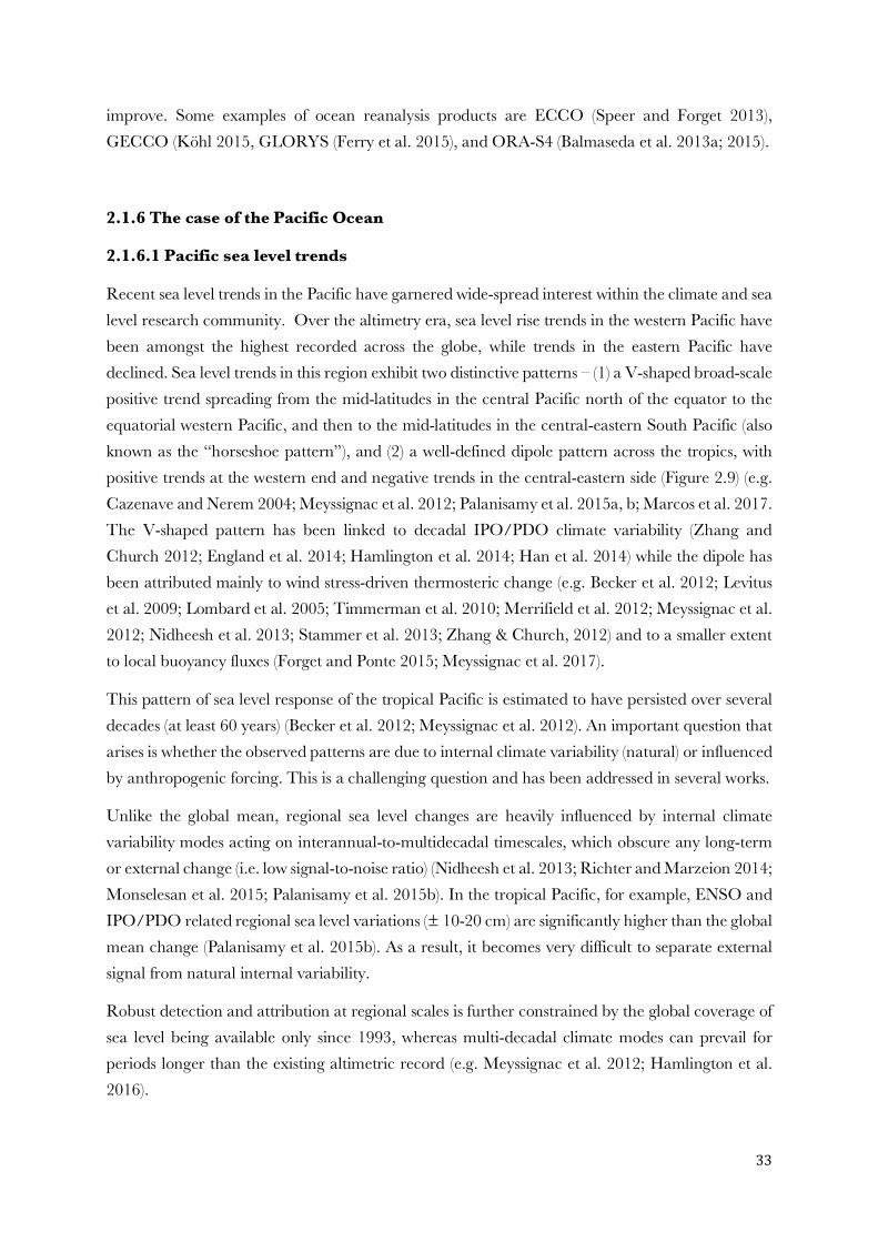
33

improve. Some examples of ocean reanalysis products are ECCO (Speer and Forget 2013), GECCO (Köhl 2015, GLORYS (Ferry et al. 2015), and ORA-S4 (Balmaseda et al. 2013a; 2015).

2.1.6 The case of the Pacific Ocean

2.1.6.1 Pacific sea level trends

Recent sea level trends in the Pacific have garnered wide-spread interest within the climate and sea level research community. Over the altimetry era, sea level rise trends in the western Pacific have been amongst the highest recorded across the globe, while trends in the eastern Pacific have declined. Sea level trends in this region exhibit two distinctive patterns – (1) a V-shaped broad-scale positive trend spreading from the mid-latitudes in the central Pacific north of the equator to the equatorial western Pacific, and then to the mid-latitudes in the central-eastern South Pacific (also known as the “horseshoe pattern”), and (2) a well-defined dipole pattern across the tropics, with positive trends at the western end and negative trends in the central-eastern side (Figure 2.9) (e.g. Cazenave and Nerem 2004; Meyssignac et al. 2012; Palanisamy et al. 2015a, b; Marcos et al. 2017. The V-shaped pattern has been linked to decadal IPO/PDO climate variability (Zhang and Church 2012; England et al. 2014; Hamlington et al. 2014; Han et al. 2014) while the dipole has been attributed mainly to wind stress-driven thermosteric change (e.g. Becker et al. 2012; Levitus et al. 2009; Lombard et al. 2005; Timmerman et al. 2010; Merrifield et al. 2012; Meyssignac et al. 2012; Nidheesh et al. 2013; Stammer et al. 2013; Zhang & Church, 2012) and to a smaller extent to local buoyancy fluxes (Forget and Ponte 2015; Meyssignac et al. 2017).

This pattern of sea level response of the tropical Pacific is estimated to have persisted over several decades (at least 60 years) (Becker et al. 2012; Meyssignac et al. 2012). An important question that arises is whether the observed patterns are due to internal climate variability (natural) or influenced by anthropogenic forcing. This is a challenging question and has been addressed in several works.

Unlike the global mean, regional sea level changes are heavily influenced by internal climate variability modes acting on interannual-to-multidecadal timescales, which obscure any long-term or external change (i.e. low signal-to-noise ratio) (Nidheesh et al. 2013; Richter and Marzeion 2014; Monselesan et al. 2015; Palanisamy et al. 2015b). In the tropical Pacific, for example, ENSO and IPO/PDO related regional sea level variations (± 10-20 cm) are significantly higher than the global mean change (Palanisamy et al. 2015b). As a result, it becomes very difficult to separate external signal from natural internal variability.

Robust detection and attribution at regional scales is further constrained by the global coverage of sea level being available only since 1993, whereas multi-decadal climate modes can prevail for periods longer than the existing altimetric record (e.g. Meyssignac et al. 2012; Hamlington et al. 2016).

34

Figure 2.9: Sea level trends in the Pacific region over the 1993–2014 period from altimetry observations (GMSL trend included). Inset shows the study sites—Suva, Lautoka, and Nouméa. In line with detection and attribution works, several “Time of Emergence” (ToE) studies have recently been conducted on regional sea level changes. ToE is defined as the time at which the external anthropogenic signal surpasses a certain detection threshold and becomes discernible from the noise of natural climate variability (i.e. favorable signal-to-noise ratio). External forcings in both steric and dynamic sea levels could be detectable by as early as the 2030s (Lyu et al. 2014) or mid-2040s (Richter and Marzeion 2014) in 50% of the world oceans. While the average ToE has been determined as at least 40 years (Jordà 2014), it can be as high as 60-80 years in regions with high interannual to decadal sea level variability, such as the tropical Pacific (Lyu et al. 2014; Richter and Marzeion 2014; Bilbao et al. 2015). These ToE studies unanimously portray that externally forced signals remain masked through longer periods in regions with strong internal variability.

Studies such as Meyssignac et al. 2012, Palanisamy et al. 2015b, and Bilbao et al. 2015 (plus references therein) have attributed sea level trends in the Pacific Ocean to internal climate variability, stating that the anthropogenic fingerprint is not yet detectable. Their conclusion is based on the high amount of noise in observations at this stage, plus the underestimation of internal variability in climate models. Nonetheless, these studies acknowledge that anthropogenic forcing

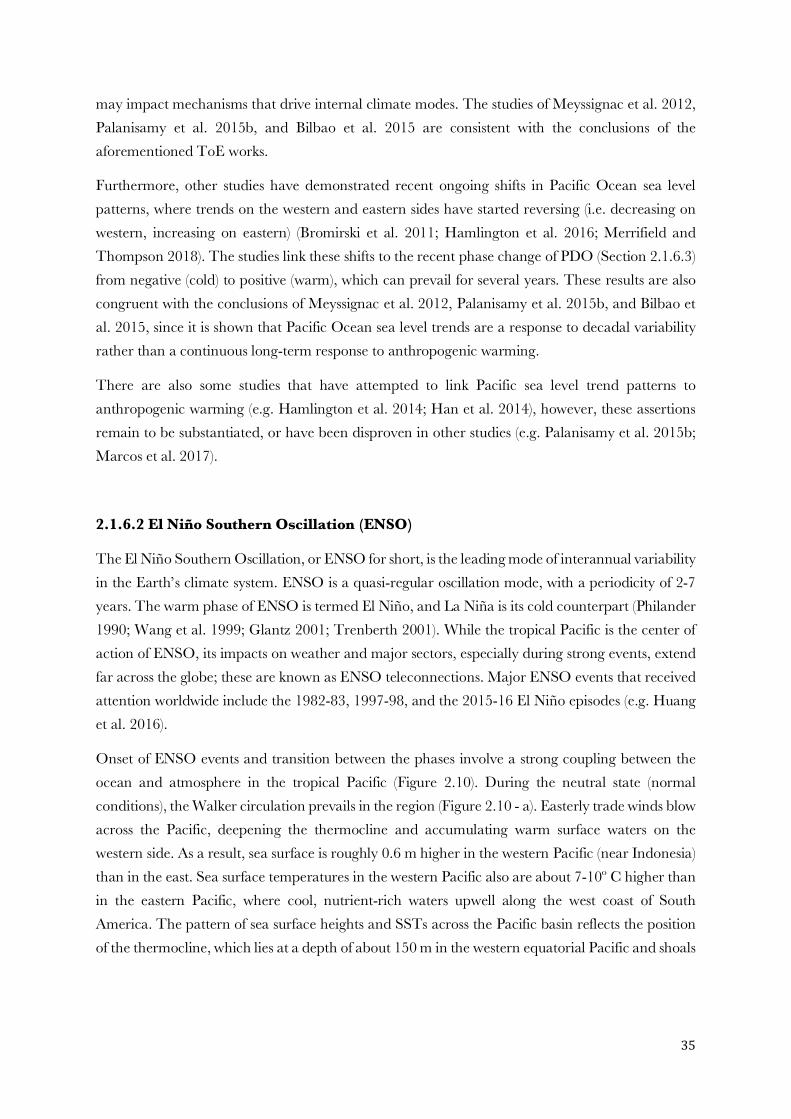
35

may impact mechanisms that drive internal climate modes. The studies of Meyssignac et al. 2012, Palanisamy et al. 2015b, and Bilbao et al. 2015 are consistent with the conclusions of the aforementioned ToE works.

Furthermore, other studies have demonstrated recent ongoing shifts in Pacific Ocean sea level patterns, where trends on the western and eastern sides have started reversing (i.e. decreasing on western, increasing on eastern) (Bromirski et al. 2011; Hamlington et al. 2016; Merrifield and Thompson 2018). The studies link these shifts to the recent phase change of PDO (Section 2.1.6.3) from negative (cold) to positive (warm), which can prevail for several years. These results are also congruent with the conclusions of Meyssignac et al. 2012, Palanisamy et al. 2015b, and Bilbao et al. 2015, since it is shown that Pacific Ocean sea level trends are a response to decadal variability rather than a continuous long-term response to anthropogenic warming.

There are also some studies that have attempted to link Pacific sea level trend patterns to anthropogenic warming (e.g. Hamlington et al. 2014; Han et al. 2014), however, these assertions remain to be substantiated, or have been disproven in other studies (e.g. Palanisamy et al. 2015b; Marcos et al. 2017).

2.1.6.2 El Niño Southern Oscillation (ENSO)

The El Niño Southern Oscillation, or ENSO for short, is the leading mode of interannual variability in the Earth’s climate system. ENSO is a quasi-regular oscillation mode, with a periodicity of 2-7 years. The warm phase of ENSO is termed El Niño, and La Niña is its cold counterpart (Philander 1990; Wang et al. 1999; Glantz 2001; Trenberth 2001). While the tropical Pacific is the center of action of ENSO, its impacts on weather and major sectors, especially during strong events, extend far across the globe; these are known as ENSO teleconnections. Major ENSO events that received attention worldwide include the 1982-83, 1997-98, and the 2015-16 El Niño episodes (e.g. Huang et al. 2016).

Onset of ENSO events and transition between the phases involve a strong coupling between the ocean and atmosphere in the tropical Pacific (Figure 2.10). During the neutral state (normal conditions), the Walker circulation prevails in the region (Figure 2.10 - a). Easterly trade winds blow across the Pacific, deepening the thermocline and accumulating warm surface waters on the western side. As a result, sea surface is roughly 0.6 m higher in the western Pacific (near Indonesia) than in the east. Sea surface temperatures in the western Pacific also are about 7-10º C higher than in the eastern Pacific, where cool, nutrient-rich waters upwell along the west coast of South America. The pattern of sea surface heights and SSTs across the Pacific basin reflects the position of the thermocline, which lies at a depth of about 150 m in the western equatorial Pacific and shoals

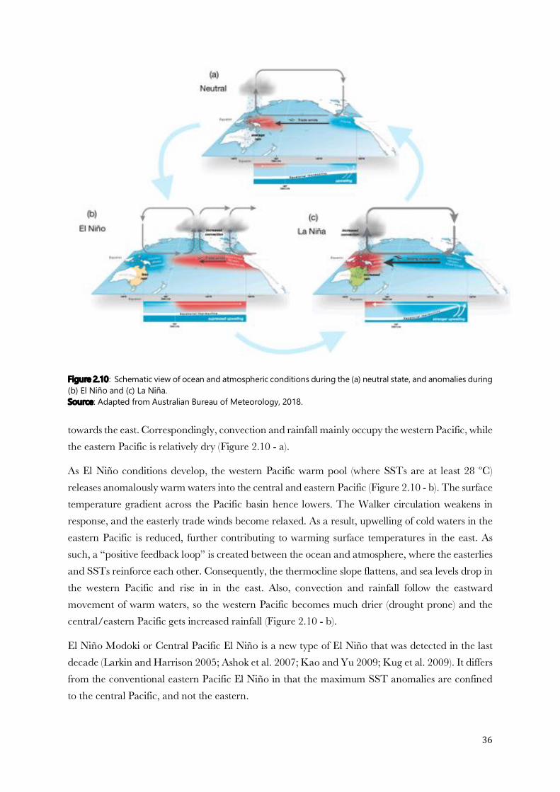
36

Figure 2.10: Schematic view of ocean and atmospheric conditions during the (a) neutral state, and anomalies during (b) El Niño and (c) La Niña. Source: Adapted from Australian Bureau of Meteorology, 2018. towards the east. Correspondingly, convection and rainfall mainly occupy the western Pacific, while the eastern Pacific is relatively dry (Figure 2.10 - a).

As El Niño conditions develop, the western Pacific warm pool (where SSTs are at least 28 ºC) releases anomalously warm waters into the central and eastern Pacific (Figure 2.10 - b). The surface temperature gradient across the Pacific basin hence lowers. The Walker circulation weakens in response, and the easterly trade winds become relaxed. As a result, upwelling of cold waters in the eastern Pacific is reduced, further contributing to warming surface temperatures in the east. As such, a “positive feedback loop” is created between the ocean and atmosphere, where the easterlies and SSTs reinforce each other. Consequently, the thermocline slope flattens, and sea levels drop in the western Pacific and rise in in the east. Also, convection and rainfall follow the eastward movement of warm waters, so the western Pacific becomes much drier (drought prone) and the central/eastern Pacific gets increased rainfall (Figure 2.10 - b).

El Niño Modoki or Central Pacific El Niño is a new type of El Niño that was detected in the last decade (Larkin and Harrison 2005; Ashok et al. 2007; Kao and Yu 2009; Kug et al. 2009). It differs from the conventional eastern Pacific El Niño in that the maximum SST anomalies are confined to the central Pacific, and not the eastern.

37

Typically, El Niño events last for 9-12 months, although longer episodes occasionally take place. Often, but not always, the warm El Niño events are followed by cool La Niña episodes, after which the ocean and atmosphere in the tropical Pacific return to neutral. La Niña conditions generally last longer than El Niño, up to 2-3 years, and take place more gradually.

During La Niña conditions, the Walker circulation strengthens and the western Pacific warm pool shifts further westwards (Figure 2.10 - c). Stronger than average easterly trade winds blow across the tropical Pacific and sea levels rise in the western end. SSTs in the central/eastern Pacific become anomalously low, and upwelling is enhanced. The surface temperature gradient across the equatorial Pacific heightens, and the thermocline steepens. Accompanying the flow of warm waters, convection and rainfall also move further west, where heavy rain and floods become frequent.

Several indices can be used to measure the phase and intensity of ENSO events (Hanley et al. 2003). The Southern Oscillation Index (SOI) is the oldest of these; it is based on the sea level pressure difference between Darwin (northern Australia) and Tahiti (French Polynesia) (e.g. Allan et al. 1991). SOI time series from 1880 to 2013 are shown in Figure 2.11. The Niño 3.4 index, which is based on regional SSTs, is also commonly used. Others include the Multivariate ENSO Index (MEI) (Wolter and Timlin 1998) and the Trans-Niño Index (TNI) (Trenberth and Stepaniak 2001).

Figure 2.11: SOI time series from 1880 to 2013. Negative SOI values correspond to El Niño conditions (blue) and positive SOI values to La Niña conditions (red). Source: NIWA 2018.

2.1.6.3 Decadal variability – IPO and PDO

The Interdecadal Pacific Oscillation (IPO) and the Pacific Decadal Oscillation (PDO) are “ENSO-like” features of the climate system that operate on decadal to multi-decadal timescales (Zhang et al. 1997; Mantua et al. 1997; Mantua and Hare 2002). IPO and PDO are distinguished from each other by their spatial coverage – while PDO is centered in the North Pacific (poleward of 20 ºN),

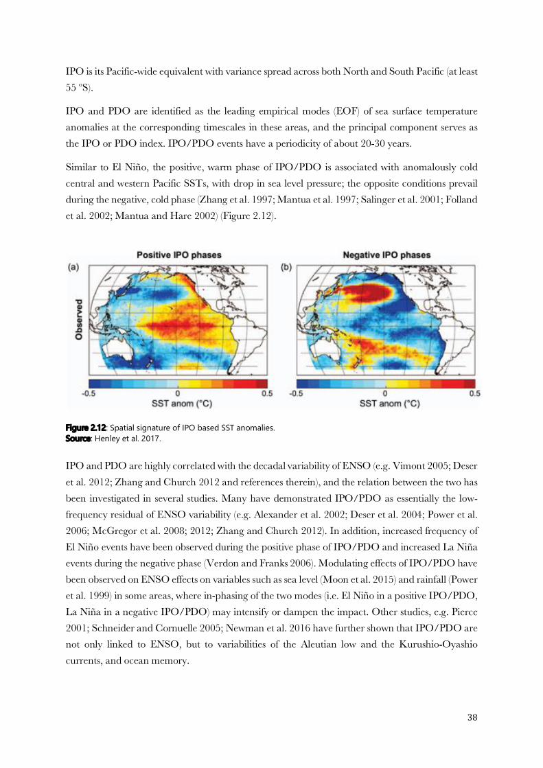
38

IPO is its Pacific-wide equivalent with variance spread across both North and South Pacific (at least 55 ºS).

IPO and PDO are identified as the leading empirical modes (EOF) of sea surface temperature anomalies at the corresponding timescales in these areas, and the principal component serves as the IPO or PDO index. IPO/PDO events have a periodicity of about 20-30 years.

Similar to El Niño, the positive, warm phase of IPO/PDO is associated with anomalously cold central and western Pacific SSTs, with drop in sea level pressure; the opposite conditions prevail during the negative, cold phase (Zhang et al. 1997; Mantua et al. 1997; Salinger et al. 2001; Folland et al. 2002; Mantua and Hare 2002) (Figure 2.12).

Figure 2.12: Spatial signature of IPO based SST anomalies. Source: Henley et al. 2017. IPO and PDO are highly correlated with the decadal variability of ENSO (e.g. Vimont 2005; Deser et al. 2012; Zhang and Church 2012 and references therein), and the relation between the two has been investigated in several studies. Many have demonstrated IPO/PDO as essentially the low-frequency residual of ENSO variability (e.g. Alexander et al. 2002; Deser et al. 2004; Power et al. 2006; McGregor et al. 2008; 2012; Zhang and Church 2012). In addition, increased frequency of El Niño events have been observed during the positive phase of IPO/PDO and increased La Niña events during the negative phase (Verdon and Franks 2006). Modulating effects of IPO/PDO have been observed on ENSO effects on variables such as sea level (Moon et al. 2015) and rainfall (Power et al. 1999) in some areas, where in-phasing of the two modes (i.e. El Niño in a positive IPO/PDO, La Niña in a negative IPO/PDO) may intensify or dampen the impact. Other studies, e.g. Pierce 2001; Schneider and Cornuelle 2005; Newman et al. 2016 have further shown that IPO/PDO are not only linked to ENSO, but to variabilities of the Aleutian low and the Kurushio-Oyashio currents, and ocean memory.

39

Phase transitions of IPO and PDO (index time series) since the late 19th century are shown in Figure 2.13. The current phase is negative, having started about 20 years ago (e.g. Hare and Mantua 2000; Deser et al. 2004).

Figure 2.13: IPO and PDO index time series from 1880 to 2016. Source: Merrifield and Thompson 2018.

2.2 Downscaling – an introduction

Climate models form the basis of understanding climate processes and variability in the present day, and serve as the primary tools for making short as well as long-term projections (predictions and projections). General circulation models (GCMs) have developed greatly since their inception in the late 1960s (Edwards 2011), with the current state-of-the-art atmosphere-ocean coupled GCMs superior to their predecessors in many ways (Flato et al. 2013). Yet, even as climate models continue to improve, simulations are far from perfect and the raw GCM output usually cannot be directly applied at local scales (Flato et al. 2013). One of the main reasons for this is the low spatial resolution of GCMs, which is typically 100 km for the ocean component (for CMIP5 models - Taylor et al. 2012). For small islands, such as those in the Pacific, this is a pronounced issue as it means that local topographical features influencing climate and weather processes (e.g. mountains, orographic details, land cover, island shape, coastal processes etc.) remain unresolved, and the model often perceives the island as part of the ocean. GCM simulations may further need additional processing because of inherent biases in the models. These are especially prominent in the tropical Pacific, with known problems in SSTs and circulation patterns, such as the double Intertropical Convergence Zone (ITCZ) (e.g. Hirota et al. 2011; Oueslati and Bellon 2015; Zhang et al. 2015; Xiang et al. 2017), zonal South Pacific Convergence Zone (SPCZ) (e.g. Brown et al. 2013; Niznik et al. 2015) and the westward extension of the equatorial cold tongue (Zheng et al. 2012; Vanniere et al. 2013; Li et al. 2016b), consequently resulting in biased climate simulations for the surrounding islands as well.

In terms of impacts on natural resources, human health, infrastructure and industry, and the associated need for better adaptation planning and risk minimization measures in vulnerable zones, it is information on regional and/or local scales that is required. This is where downscaling comes

40

in. Downscaling refers to the process of inferring local scale (high resolution) information from low resolution variables or simulations (Figure 2.14). Downscaling can thus be interpreted as a means of bridging the gap between the low resolution of GCMs and the high resolution information that is needed for practical applications (Benestad et al. 2007; Brown et al. 2008; Boulanger et al. 2010; Flato et al. 2013).

Figure 2.14: The concept of spatial downscaling. The increase in resolution often refers to both spatial and temporal scales. Downscaling of large-scale information can be broadly classified into two categories: (1) dynamical, and (2) statistical (empirical), which are discussed in the following sections.

2.2.1 Dynamical downscaling

Dynamical downscaling uses a high resolution regional climate model (RCM), containing finer level information (e.g. additional physical processes, geophysical features, regional tuning etc.), that is driven by large-scale information (termed as “boundary conditions”) from a GCM (Figure 2.14). The RCM generally has spatial resolution ranging between 50 to 10 km, or less, and is better able to incorporate the local topography, landscape, terrestrial features, and possibly local atmospheric processes as well. Thus, the local climate simulations are more detailed, with possible improvement in representation of weather extremes. The results are sensitive to both the forcing GCM as well as the high resolution RCM. Dynamical downscaling can be conducted as (1) limited time slice experiments (20-30 years), (2) limited-area models run over a specified area, or (3) stretched grid models with fine resolution over the area of interest and coarse resolution elsewhere. Examples of dynamical downscaling studies include the CLARIS project (Menéndez et al. 2010), NARCCAP (Mearns et al. 2009), CORDEX (Dosio and Panitz 2016; Giorgi and Gutowski 2015), AMMA (Redelsperger et al. 2006), and PRUDENCE (Christensen et al. 2007a), amongst many others.

41

Dynamical downscaling methods are able to generate very high resolution climate simulations (up to 10 km and higher), while largely preserving physical relationships between variables. In addition to coupled climate models, dynamical downscaling can be applied to ocean-only, atmosphere only, or biogeochemistry-only models.

The main disadvantage of dynamical downscaling, however, is the highly intensive computational demand, which limits the number of overall simulations (GCMs, emission scenarios, time periods) (Christensen et al., 2007b; Australian Bureau of Meteorology and CSIRO 2011; Flato et al. 2013).

2.2.2 Statistical downscaling

Statistical, or empirical downscaling, on the other hand, uses cross-scale relationships derived from observed data and applies these to climate model data (von Storch et al. 2000; Benestad et al. 2007; Christensen et al. 2007b) (Figure 2.14). Statistical downscaling methods can include simple interpolation of GCM simulations to the site of interest, or more complex statistical models that relate large scale variables to local parameters (Benestad et al. 2007). Here, the statistical model requires high quality observational records extending over decades for calibration and verification, and the results are sensitive to the chosen GCM or other large-scale predictor variables. Statistical downscaling techniques may also be developed between existing records of predictor (input data for statistical model, typically large-scale parameters) and predictand (output data, typically small scale) variables from observations and reanalysis, and then applied to GCMs. There are various approaches to statistical downscaling, including linear methods such as multivariate regression (e.g. Khalili et al. 2011; Bhowmik et al. 2017), canonical correlation analysis (CCA) (e.g. Busuioc et al. 2008; Werner et al. 2013), and singular vector decomposition (SVD) analysis (e.g. Paul et al. 2008; Diaconescu and Laprise 2012; Khalili et al. 2018), and non-linear methods such as analog models (e.g. Teng et al. 2012; Pierce et al. 2014), cluster analysis (classification methods) (e.g. Wang et al. 2013; Daloz et al. 2015), and neural networks (e.g. Mendez and Marengo 2010; Dorji et al. 2017). Each method is constructed to best suit the type of relationship being modeled between the predictors and predictand, and may often be combined with pre-processing of data using procedures such as Empirical Orthogonal Function (EOF) analysis. Additionally, statistical downscaling can be combined with dynamical models for optimization and robustness, such as in the STARDEX downscaling project for extremes in Europe (STARDEX 2005). Unlike dynamical techniques, statistical downscaling is computationally inexpensive. The main drawback associated with statistical methods is that it assumes that the cross-scale relationships derived between large-scale climate patterns and the local climate remain constant, which may not always apply in a perturbed system.

42

2.2.3 Downscaling method used – MLR

In this thesis, a statistical downscaling model for island sea levels at the study sites is constructed using a multiple linear approach (MLR), with selected oceanic and atmospheric variables serving as regressors. This approach was selected given its practical advantages; regression methods are relatively easy to implement and require low computational resources, making them more easily transferable to local communities.

The MLR approach has been used in several statistical downscaling studies on sea level, such as Sterlini et al. 2016, Dangendorf et al. 2013a, 2014, and Calafat and Chambers 2013. In some studies, such as Albrecht and Weisse 2012, and Dangendorf et al. 2013b, the MLR method is combined with EOFs.

The MLR methodology used is detailed in Chapter 3.

2.3 Study sites

The western South Pacific is home to numerous island nations. These include countries such as Vanuatu, the Solomon Islands, Tuvalu, New Caledonia, Wallis and Futuna, Fiji, and Tonga. Of these, study sites were selected from Fiji – Suva and Lautoka, and New Caledonia – Nouméa to conduct the MLR downscaling experiments. The study sites are marked in Figures 2.15 and 2.16. These sites were selected on the basis of their location in the western Pacific, an island region already experiencing the threats of sea level rise, which is much likely to exacerbate in future (Webb and Kench 2010; Hallegatte et al. 2013; Nurse et al. 2014; Wong et al. 2013; Neumann et al. 2015; Albert et al. 2016; Hinkel et al. 2019). Relocation of coastal communities to higher ground due to frequent inundation, contamination of freshwater lenses/saltwater intrusion, flash floods, and increased frequency of extreme sea levels are some of the examples that have become common in these island nations over the recent years (e.g. Limalevu et al. 2010; OCHA—United Nations 2014; McNamara & Jacot Des Combes 2015; SPC 2016). Fiji and New Caledonia from this region were chosen in particular as the thesis was conducted in collaboration with research institutions based in the two island nations (USP - Suva, IRD - Nouméa).

Both Fiji (176-183ºE, 16-20ºS) and New Caledonia (158-174ºE, 17-23ºS) lie in Melanesia, which is one of the three main ethnogeographic subregions of the Pacific. New Caledonia has one main island, the Grand Terre, and several smaller islands distributed across four island groups. Fiji has two main islands, Viti Levu and Vanua Levu, with over 300 islands in total (about one third inhabited).

Situated between the tropic of Capricorn and the Equator, both Fiji and New Caledonia have warm, humid climates throughout the year, influenced greatly by the south easterly trade winds.

43

Figure 2.15: Map of the Fiji Islands, with study sites Suva and Lautoka marked. Source: SPC 2014a.

Figure 2.16: Map of New Caledonia, with study site Nouméa marked. Source: SPC 2014b.

44

The orographic effect occurs on the mountainous islands, where the eastern sides are wetter and western sides drier (Leroy 2006; Lal et al. 2008; Cavarero et al. 2012).

Interannual variability in the region is largely governed by ENSO, which is associated with droughts during El Niño events and heavy rainfalls/flooding during La Niñas. Depending on the severity of the event, these ENSO episodes hold great consequences for the interrelated sectors of food and water security, agriculture, fisheries, economy, and health (vector-borne diseases) (Leroy 2006; Lal et al. 2008; Australian Bureau of Meteorology and CSIRO 2011; Cavarero et al. 2012). Notable El Niño events from the past include the 1982-83, 1997-98, and 2015-16 events, which were associated with droughts in the region. Extreme events affecting Fiji and New Caledonia are tropical cyclones, floods, and storm surges, of which the former has the most destructive and widespread impacts.

As global warming progresses and western Pacific sea levels gradually rise, both countries are becoming increasingly threatened by inundation, salt water intrusion, ocean acidification, and changing weather patterns (e.g. off-season cyclone Donna striking New Caledonia in May 2017). Sustainable development, carbon neutrality, awareness raising, and capacity and resilience building are some of the measures these island nations are undertaking to adapt to recent climatic changes (COP23 2018a, b; PCCP 2018) The present downscaling study can be perceived as a step in the direction of the capacity and resilience building initiatives.

2.4 Synthesis and MLR framework

Bringing into perspective all the information provided in this chapter, sea level at a given location can be interpreted as a sum of various processes acting on different spatial and temporal scales (Figure 2.17). Since the timescales of all the processes involved are different, their relative contribution to sea level depends essentially on the timescale being considered – seasonal, interannual, decadal/multi-decadal, long-term, extremes (under contemporary sea level), historical, etc. Historical sea level changes have been driven mainly by tectonic processes and glacial-interglacial cycles. In the present day, global mean sea level is rising primarily due to thermal expansion of water, and melt of glaciers and ice sheets induced by global warming (anthropogenic). On regional to local scales, natural internal climate variability (e.g. ENSO, PDO/IPO) still plays a deterministic role.

For contemporary sea level changes and future projections to guide necessary adaptation and risk minimization measures, climate models serve as the primary source of information. While climate models are helpful at large scales, they have limited applicability at local scales owing to low resolution. Additionally, they have known biases in the Pacific region, rendering the models an inefficient source of information for islands in the region. Here, downscaling, whereby high

45

resolution, local scale information is extracted from low resolution climate simulations, plays a crucial role. The two main types of downscaling are dynamical and statistical.

In this thesis, sea level at the study sites Suva, Lautoka (Fiji), and Nouméa (New Caledonia) in the southwest Pacific are reconstructed using a statistical downscaling model, one that employs a multiple linear regression (MLR) technique. The central framework of statistical downscaling is that sea level at any particular site is a function of the global, regional, and local drivers. The model in this thesis is configured to simulate the regional and local drivers (global mean adjusted for), which are represented via a combination of oceanic and atmospheric variables (predictors). Selection of these variables is based on existing knowledge of sea level dynamics in the southwest Pacific, focusing on sea level variability on interannual-to-decadal scales, plus trend. The MLR model computes an optimum calibration of the set of predictor variables, producing a close estimate of the observed sea level.

It is envisaged that the MLR model developed in this thesis can be applied with climate models to extract local scale sea level projections and thus be utilized in refining climate adaption measures in the region.

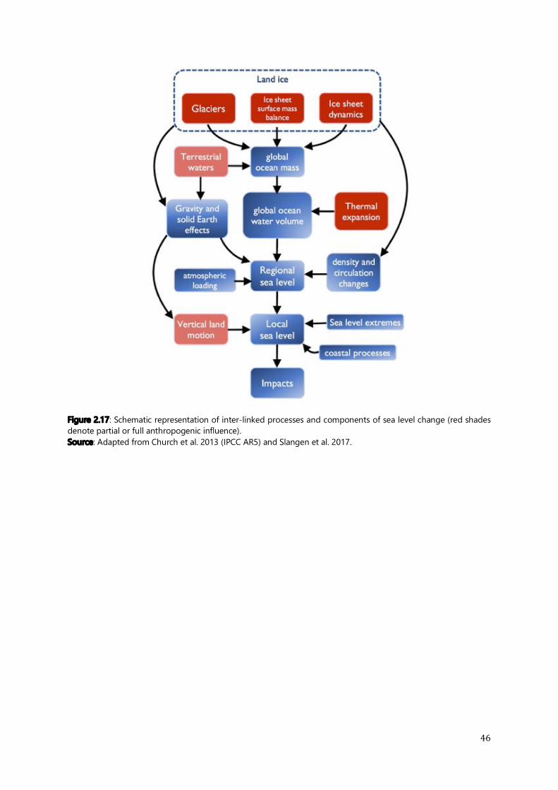
46

Figure 2.17: Schematic representation of inter-linked processes and components of sea level change (red shades denote partial or full anthropogenic influence). Source: Adapted from Church et al. 2013 (IPCC AR5) and Slangen et al. 2017.

47

Chapter 3

Methodology and datasets Part 1 - Methodology 3.1 Multiple linear regression analysis ........................................................ 49

3.1.1 The MLR model ........................................................................................................ 49 3.1.2 Stepwise selection of regressors .................................................................................. 50 3.1.3 Metrics for the evaluation of MLR models ................................................................ 52

3.2 Interannual-to-decadal sea level variations and trends – Study period, data preprocessing and filtering .................................................................... 52

Part 2 – Statistical downscaling datasets and experiments 3.3 Island sea level predictands .................................................................. 53

3.3.1 Tide gauge records .................................................................................................... 53 3.3.2 ORA-S4 reanalysis sea level ...................................................................................... 56 3.3.3 Altimetric sea level ..................................................................................................... 56

3.4 Potential predictors ............................................................................ 57 3.4.1 Selection of regressor variables – direct and dynamic MLR approaches ............... 57 3.4.2 Regressor datasets...................................................................................................... 58

3.4.2.1 Mass change estimate – GRACE .................................................................... 58 3.4.2.2 ERA-Interim data (Wind, SST, SLP fields) .................................................... 59 3.4.2.3 ORA-S4 Steric fields ....................................................................................... 59

3.5 Rossby wave model ............................................................................. 62 3.6 MLR experiments ............................................................................... 63

3.6.1 Preliminary analysis – Steric plus mass MLR models (2003-2014) ........................... 63 3.6.2 Wind stress curl (Rossby wave model) dominated MLR models (1988-2014) .......... 66

3.6.2.1 Treatment of the GMSL trend in the predictand ........................................... 67 3.6.3 A simplified approximation of the wind stress curl proxy ......................................... 70

3.7 Stationarity test .................................................................................. 71 3.8 Summary ........................................................................................... 73

49

3. Methodology and datasets

This chapter presents the MLR methodology and datasets used in the analysis. The MLR methodology is presented first, detailing the statistical downscaling model, stepwise regression function to extract significant regressors, and evaluation metrics for the MLR model calibrated. The study period, initial preprocessing steps, such as treatment of trends and seasonal cycles, types of filters used to isolate the frequency of sea level variations being studied (interannual-to-decadal), are described.

The second section focuses on the MLR experiments and predictand/regressor datasets used. It describes the different sets of MLR experiments conducted given different combination of regressors and the periods over which they were available. The Rossby wave model, which is an integral part of the study methodology, is presented in this section.

After describing the different experiments, a stationarity test assessing the applicability of the MLR models developed to future projections of island sea levels is presented at the end.

Supplementary material not included in this chapter is provided in the Appendix, and made reference to where needed.

Part 1 – Methodology 3.1 Multiple linear regression analysis

3.1.1 The MLR model

The statistical downscaling model for island sea levels presented in this thesis is constructed using multiple linear regression (e.g. Sterlini et al. 2016, Dangendorf et al. 2013a, 2014). In this model, the predictors or regressors are a combination of oceanic and atmospheric variables characterizing island sea level dynamics in the western Pacific region.

The MLR model used here for sea level anomalies, sla, at a given time, t, can be expressed as:

"#$("&'(, ') = ∑ ∝. /.01., 2., ' − '.4. + 6("&'(, ') - - - - - - - - - - - - - - - - - - (3.1)

where:

site = the geographical site studied (Suva, Lautoka or Nouméa), ∝i = site-specific regression coefficients, Pi = potential predictors (representing sea level change drivers) averaged over a site-specific (xi,yi) spatial area, ti = temporal lag, and

50

ε = site-specific residual (which is not part of the MLR model and represents the difference between the island and modeled sea level time series). The sea level time series being modeled is called the predictand or island sea level hereafter. Predictands

The predictands in the MLR model were sea level anomaly time series (1993-2012 baseline) for each of the study sites. The predictand sea levels were from (1) ORA-S4 and (2) tide gauge records.

Thus, each MLR experiment was conducted on two sets of predictands – reanalysis and in situ sea levels (Section 3.3). Regressor variables

The regressor variables, depending on the specific MLR experiment, were anomaly time series of sea level predictors (direct or dynamic mechanism-based predictors - see Sections 3.4.1, 3.6) with respect to the calibration period for the MLR model as the baseline. The regressor anomaly time series were hence re-adjusted in experiments spanning different time frames.

3.1.2 Stepwise selection of regressors

A classic problem encountered in most MLR approaches arises from cross-correlations between regressors; this is also known as multi-collinearity.

While regressors which are not statistically independent from each other have little effect on the overall modeled fit, the efficiency of the MLR model is compromised in terms of how effective individual regressors are at modulating the predictand, i.e. isolating the relationship between the two – a key aspect in the MLR methodology. With multi-collinearity, the error associated with each regressor increases and is spread over a larger confidence estimate. As a result, it becomes difficult to understand the relative importance of a particular variable in the model. Furthermore, MLR models can be highly sensitive to minor changes in regressor datasets; these can lead to larges changes in how the model is calibrated, even resulting in reversal of coefficient signs.

The potential regressors for the MLR model used here are a set of oceanic and atmospheric variables (Section 3.4), all of which are interlinked components of the climate system in a common region. Thus, although a certain degree of covariance is indeed expected between the individual regressors, the model has to be developed such that the selected regressors are statistically distinct from each other (i.e. regressor-dependent model skill is optimized).

For this, an interactive stepwise regression function based on the statistical significance (95% confidence interval) of a regressor in the MLR model was used.

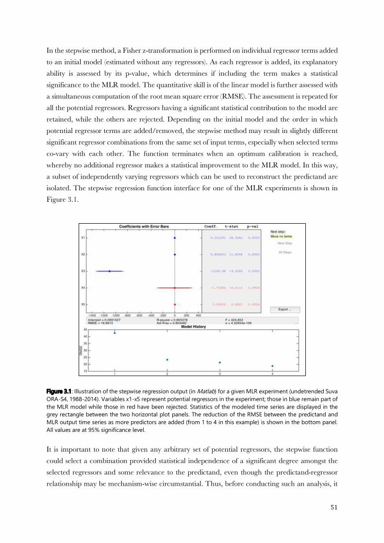
51

In the stepwise method, a Fisher z-transformation is performed on individual regressor terms added to an initial model (estimated without any regressors). As each regressor is added, its explanatory ability is assessed by its p-value, which determines if including the term makes a statistical significance to the MLR model. The quantitative skill is of the linear model is further assessed with a simultaneous computation of the root mean square error (RMSE). The assessment is repeated for all the potential regressors. Regressors having a significant statistical contribution to the model are retained, while the others are rejected. Depending on the initial model and the order in which potential regressor terms are added/removed, the stepwise method may result in slightly different significant regressor combinations from the same set of input terms, especially when selected terms co-vary with each other. The function terminates when an optimum calibration is reached, whereby no additional regressor makes a statistical improvement to the MLR model. In this way, a subset of independently varying regressors which can be used to reconstruct the predictand are isolated. The stepwise regression function interface for one of the MLR experiments is shown in Figure 3.1.

Figure 3.1: Illustration of the stepwise regression output (in Matlab) for a given MLR experiment (undetrended Suva ORA-S4, 1988-2014). Variables x1-x5 represent potential regressors in the experiment; those in blue remain part of the MLR model while those in red have been rejected. Statistics of the modeled time series are displayed in the grey rectangle between the two horizontal plot panels. The reduction of the RMSE between the predictand and MLR output time series as more predictors are added (from 1 to 4 in this example) is shown in the bottom panel. All values are at 95% significance level. It is important to note that given any arbitrary set of potential regressors, the stepwise function could select a combination provided statistical independence of a significant degree amongst the selected regressors and some relevance to the predictand, even though the predictand-regressor relationship may be mechanism-wise circumstantial. Thus, before conducting such an analysis, it

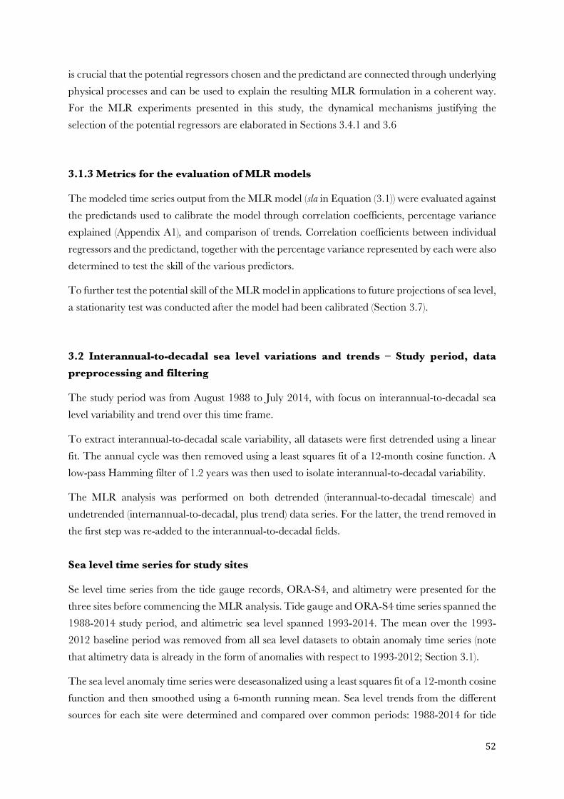
52

is crucial that the potential regressors chosen and the predictand are connected through underlying physical processes and can be used to explain the resulting MLR formulation in a coherent way. For the MLR experiments presented in this study, the dynamical mechanisms justifying the selection of the potential regressors are elaborated in Sections 3.4.1 and 3.6

3.1.3 Metrics for the evaluation of MLR models

The modeled time series output from the MLR model (sla in Equation (3.1)) were evaluated against the predictands used to calibrate the model through correlation coefficients, percentage variance explained (Appendix A1), and comparison of trends. Correlation coefficients between individual regressors and the predictand, together with the percentage variance represented by each were also determined to test the skill of the various predictors.

To further test the potential skill of the MLR model in applications to future projections of sea level, a stationarity test was conducted after the model had been calibrated (Section 3.7).

3.2 Interannual-to-decadal sea level variations and trends – Study period, data preprocessing and filtering

The study period was from August 1988 to July 2014, with focus on interannual-to-decadal sea level variability and trend over this time frame.

To extract interannual-to-decadal scale variability, all datasets were first detrended using a linear fit. The annual cycle was then removed using a least squares fit of a 12-month cosine function. A low-pass Hamming filter of 1.2 years was then used to isolate interannual-to-decadal variability.

The MLR analysis was performed on both detrended (interannual-to-decadal timescale) and undetrended (internannual-to-decadal, plus trend) data series. For the latter, the trend removed in the first step was re-added to the interannual-to-decadal fields. Sea level time series for study sites

Se level time series from the tide gauge records, ORA-S4, and altimetry were presented for the three sites before commencing the MLR analysis. Tide gauge and ORA-S4 time series spanned the 1988-2014 study period, and altimetric sea level spanned 1993-2014. The mean over the 1993-2012 baseline period was removed from all sea level datasets to obtain anomaly time series (note that altimetry data is already in the form of anomalies with respect to 1993-2012; Section 3.1).

The sea level anomaly time series were deseasonalized using a least squares fit of a 12-month cosine function and then smoothed using a 6-month running mean. Sea level trends from the different sources for each site were determined and compared over common periods: 1988-2014 for tide

53

gauges and ORA-S4; 1993-2014 for tide gauges, ORA-S4, and altimetry. Uncertainties in trends were expressed as the formal error of the least-squares linear regression, as in Becker et al. 2012 and 2014. Correlation coefficients between island sea levels from the different data sources were computed over common periods (Chapter 5 – Section 5.1).

Part 2 – Statistical downscaling datasets and experiments 3.3 Island sea levels predictands

Local sea levels were taken from 3 different sources: tide gauge records, satellite altimetry, and the ORA-S4 reanalysis product.

Different sources for the local sea levels have been used in attempts to obtain a more robust interpretation of the MLR experiment results, while still acknowledging the limitations associated with a particular product. Each dataset has its inherent set of advantages and limitations, with the underlying causes of bias in one product usually serving as the advantage in another. For example, although tide gauge records provide site-specific, high resolution data on local sea level variations, some extending back to the late 19th century (Mitchum et al. 2010; Holgate et al. 2013), they are highly susceptible to vertical land motion and instrumental error (Chapter 2 – Section 2.1.5.1). Additionally, most tide gauge records have missing data/gaps. Altimetry, on the other hand, offers a more consistent measurement of absolute sea level around the globe and is not affected by vertical land motion (Chapter 2 – Section 2.1.5.2). However, it has a limited time frame for studying long-term sea level variations. Reanalysis products have the advantage of being able to provide dynamically consistent estimates because they assimilate observational records and combine these with a numerical ocean model that solves the equations of ocean dynamics (Chapter 2 – Section 2.1.5).

The different datasets for island sea levels used in this study are described below. Of these, the tide gauge and ORA-S4 sea levels were used as the predictands in the MLR model, the focus of the study. The use of altimetric data was limited only to comparisons between island sea level time series from the different sources (Chapter 5 – Section 5.1), as the dataset (1993 onwards) does not extend as far back as the start of study period (1988-2014).

3.3.1 Tide gauge records

Monthly mean Revised Local Reference (RLR) tide gauge records for Suva and Lautoka were retrieved from the Permanent Service for Mean Sea level (PSMSL) (Holgate et al. 2013; PSMSL 2016).

54

Site Grid location PSMSL

station ID Duration

% of gap (max. length in

consecutive months)

Suva 178.42 °E, 18.14 °S 1327 Oct 1972 – Dec 2014 6 (6)

Lautoka 177.44 °E, 17.60 °S 1805 Nov 1992 – Dec 2014 0.4 (1)

Nouméa 166.43 °E, 22.30 °S - Feb 1967 – Dec 2014 2 (11)

Table 3.1: Tide gauge station data for Suva, Lautoka, and Nouméa, with longitude/latitude coordinates, data duration, and percentage of missing data. For Nouméa, a merged sea level series from sites Chaleix and Numbo was used (Aucan et al. 2017). Details on these tide gauge records are presented in Table 3.1. Additionally, tide gauge locations and the nearest GPS stations at the sites are illustrated in Figures 3.2-3.4.

All missing values were filled in using linear interpolation to obtain a continuous time series and anomalies were computed with respect to the 1993-2012 period (as for satellite altimetry, see Section 3.3.3). Anomalies were adjusted for the inverted barometer (IB) effect (Wunsch and Stammer 1997) using sea level pressure anomalies from the ERA-Interim dataset. Site-specific anomalies were computed by removing the global mean of the sea level pressure anomalies from the local pressure time series and then dividing by the local gravity to obtain the net IB effect acting on a particular grid point (Wunsch and Stammer 1997).

No additional correction was applied to the tide gauge sea level time series for vertical land motion, but information provided by PSMSL and related literature (e.g. Aucan et al. 2017; Mörner and Klein 2017) were used to explain inconsistencies in trends relative to altimetry and reanalysis data (Chapter 5 – Section 5.1), and to the overall performance of the MLR model developed (Chapter 5 – Section 5.2). Reported issues with tide gauges at the study sites

For the Fiji sites, Mörner and Klein 2017 reported that the tide gauges at Suva (Figure 3.2) and Lautoka (Figure 3.3) are located in unstable areas that are highly prone to sediment compaction. The Suva tide gauge has been moved three times and as a result has recorded sea level measurements for different locations. The current Suva tide gauge is placed in a heavy harbor construction area as well, which most likely exacerbates the compaction and subsidence processes. The location of the Suva GPS station is not very relevant to the tide gauge and has been constructed on gently dipping bedrock (Figure 3.2 - c). Classified as non-robust, the Suva GPS station was deactivated in 2002.

The GPS station at Lautoka is also located unfavorably with respect to the tide gauge (Figure 3.3), and shows ambiguous vertical land motion rates overall. Both the Suva and Lautoka tide gauges have been affected by earthquakes in the past, which creates additional complications (Mörner and Klein 2017).

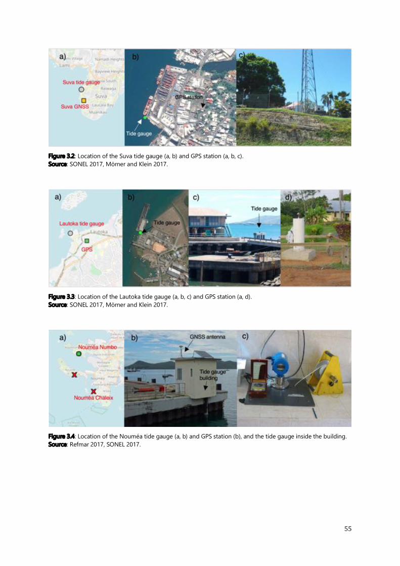
55

Figure 3.2: Location of the Suva tide gauge (a, b) and GPS station (a, b, c). Source: SONEL 2017, Mörner and Klein 2017.

Figure 3.3: Location of the Lautoka tide gauge (a, b, c) and GPS station (a, d). Source: SONEL 2017, Mörner and Klein 2017.

Figure 3.4: Location of the Nouméa tide gauge (a, b) and GPS station (b), and the tide gauge inside the building. Source: Refmar 2017, SONEL 2017.

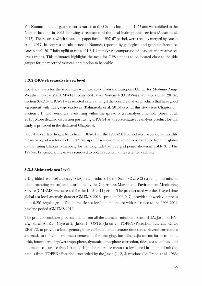
56

For Nouméa, the tide gauge records started at the Chaleix location in 1957 and were shifted to the Numbo location in 2003 following a relocation of the local hydrographic services (Aucan et al. 2017). The records, which existed on paper for the 1957-67 period, were recently merged by Aucan et al. 2017. In contrast to subsidence at Nouméa reported by geological and geodetic literature, Aucan et al. 2017 infer uplift at rates of 1.3-1.4 mm/yr via comparison of absolute and relative sea levels trends. This mismatch highlights the need for GPS stations to be located close to the tide gauges for the recorded vertical land motion to be viable.

3.3.2 ORA-S4 reanalysis sea level

Local sea levels for the study sites were extracted from the European Center for Medium-Range Weather Forecasts’ (ECMWF) Ocean ReAnalysis System 4 (ORA-S4) (Balmaseda et al. 2013a; Section 3.4.2.3). ORA-S4 was selected as it is amongst the ocean reanalysis products that have good agreement with tide gauge sea levels (Balmaseda et al. 2015) used in this study (see Chapter 5 – Section 5.1), with steric sea levels lying within the spread of a reanalysis ensemble (Storto et al. 2015). More detailed discussion portraying ORA-S4 as a representative reanalysis product for this study is provided in the dedicated Chapter 4.

Global sea surface height fields from ORA-S4 for the 1988-2014 period were accessed as monthly means at a grid resolution of 1º x 1º. Site-specific sea level time series were extracted from the global dataset using bilinear remapping for the longitude/latitude grid points shown in Table 3.1. The 1993-2012 temporal mean was removed to obtain anomaly time series for each site.

3.3.3 Altimetric sea level

2-D gridded sea level anomaly (SLA) data produced by the Ssalto/DUACS system (multi-mission data processing system) and distributed by the Copernicus Marine and Environment Monitoring Service (CMEMS) was accessed for the 1993-2014 period. The product used was the delayed time global sea level anomaly dataset (CMEMS 2018 - product 008-047), provided at weekly intervals on a 0.25° regular grid. The altimetric sea level anomalies are with reference to the 1993-2012 baseline period (CMEMS 2018).

The product combines processed data from all the altimeter missions - Sentinel-3A, Jason-3, HY-2A, Saral/AltiKa, Cryosat-2, Jason-1, OSTM/Jason-2, TOPEX/Poseidon, Envisat, GFO, ERS1/2, to provide a homogenous, inter-calibrated and accurate time series. Several corrections are made to the altimetric measurements before merging, including adjustments for instrument, orbit, ionosphere, dry/wet troposphere, dynamic atmosphere correction, tides, sea state bias, and the mean sea surface (Pujol et al. 2016). The reference mean sea level used in the multi-mission data is from TOPEX/Poseidon, succeeded by the Jason (1, 2, 3) missions (Le Traon et al. 1988;

57

CMEMS 2018).

The weekly altimetric data was regridded to monthly averages for consistency with the other datasets used in the study. Sea level anomalies for the study sites were extracted from the global dataset using distance weighted remapping for the corresponding longitude/latitude coordinates of the tide gauge records (Table 3.1).

3.4 Potential predictors

3.4.1 Selection of regressor variables – direct and dynamic MLR approaches

Sea level change can be interpreted essentially as a change in water volume, induced by either variations in mass (barystatic component; Church et al. 2013; Gregory et al. 2013) and/or density (steric component) of the water column. From a mechanistic perspective considering ocean-atmosphere dynamics, the steric and mass changes leading to overall sea level change can be attributed to specific processes at work (e.g. Nidheesh et al. 2013; Stammer et al. 2013; Forget and Ponte 2015; Meyssignac et al. 2017)

So depending on the perspective taken of island sea level – direct (i.e. static) or dynamic, the potential regressors would be different.

Thus, in the first or preliminary set of MLR experiments, the potential regressors were taken directly as the steric and mass components of island sea level (Section 3.6.1).

In the second and main set of MLR experiments, the prevalent climate drivers and circulation patterns determining the variation of the steric and mass components on regional to local scales was considered. The selection of the second set of potential regressors was based on a more mechanistic approach that considers ocean dynamics and processes occurring at these spatial scales (Section 3.6.2).

Steric changes can be due to surface buoyancy fluxes, mixing, and adiabatic motions of the isopycnals caused by adjustments to wind-driven circulation (Piecuch and Ponte 2011; Meyssignac et al. 2017). Wind stress curl produces divergence or convergence of the surface layer (Ekman pumping), which is balanced by vertical “heaving” of the thermocline. Heaving can induce changes in the vertical stratification and heat content of the water column (e.g. Huang 2015).

At interannual-to-decadal timescales, the thermosteric sea level variability in the tropics is mostly induced by the internal reorganization of ocean water masses in response to the wind stress curl forcing (Wyrtki 1975; Qiu and Chen 2006; Timmerman et al. 2010; McGregor et al. 2012; Stammer et al. 2013). Propelled by wind stress curl anomalies, westward flowing Rossby waves modulate the thermocline depth as they propagate across the Pacific basin, generating changes in the thermosteric sea level at the western end. Based on previous studies (e.g. Timmermann et al., 2010; McGregor et al., 2012; Nidheesh et al., 2013; Forget and Ponte 2015; Meyssignac et al.

58

2017), wind stress curl is therefore considered as the dominant predictor of thermosteric sea level, and hence of sea level in the region.

The remaining thermosteric sea level variability is due to buoyancy forcing at the sea surface and to intrinsic ocean variability (Meyssignac et al. 2017). To capture thermosteric sea level variability induced by surface heat forcing, local SST was taken as a potential predictor (Meyssignac et al. 2017). The other predictors included wind stress (τx, τy) in the vicinity of the study site, representing the wind set-up, and the halosteric component for salinity changes and surface freshwater fluxes.

3.4.2 Regressor datasets

3.4.2.1 Mass change estimate – GRACE

The Gravity recovery and Climate Experiment (GRACE), launched in early 2002 allowed the first ever measurements of global spatial and temporal variations in Earth’s gravity field (Tapley et al. 2004; Ramillien et al. 2016). GRACE consists of two identical satellites on the same orbital plane, separated by about 220 km. The distance between the two satellites varies in response to the differences in gravitation acceleration experienced across the trajectory and is measured by radar telemeter. Variations in the Earth’s gravity field arise from uneven mass distribution at the crust, particularly due to surface waters which change more rapidly than the Earth’s interior.

In oceanography, GRACE has revolutionized the estimation of ocean bottom pressure as ice mass is lost from glaciers and ice-sheets and added to the ocean (Frappart et al. 2016).

Ocean mass change estimates over the 2003-2014 period were extracted from an ensemble of 720 GRACE solutions computed from 5 raw GRACE solutions (provided by CSR – Center for Space Research, GFZ - GeoforschungsZentrum, JPL - Jet Propulsion Laboratory, GRGS - Groupe de Recherche de Geodesie Spatiale, and TUG - Graz University of Technology). The dataset extends from late 2002 onwards. The product uses different post processing parameters for the geocenter motion correction, Earth oblateness correction, filtering, leakage correction, and glacial isostatic adjustment (Carret et al. 2017). The spread (1.65 sigma) around the ensemble mean of the mass change estimates is used as an estimate of uncertainty.

The product was accessed as a 1°x1° global dataset over the available duration (2003-2014), and the global mean of the ensemble was taken as the estimate of local ocean mass change for all three study sites - Suva, Lautoka, and Nouméa (details in Section 3.6.1).

59

3.4.2.2 ERA-Interim data (Wind, SST, SLP fields)

The ERA-Interim reanalysis

ERA-Interim is the ECMWF’s global atmospheric reanalysis product (Dee et al. 2011; ERA-Interim 2016). It extends back in time until 1979 and is continuously updated in near real-time. ERA-Interim is a third-generation reanalysis product, successor to ERA-40 (Kållberg et al. 2007) and ERA-15 (Shea et al. 2016). The reanalysis is produced using the ECMWF’s IFS (Integrated Forecast System) model and uses a sequential data assimilation scheme (Dee et al. 2011).

ERA-Interim provides high resolution, consistent set of climate data on spatial and temporal scales, with improved performance in features such as low frequency variability and stratospheric circulation relative to precursor reanalysis products. Known biases include intensified hydrological cycle over the oceans, overestimated temperatures and humidity estimates in the Artic, and issues with cloud cover (Dee et al. 2011). While acknowledging these biases, ERA-Interim data used in various studies in the Pacific region has efficiently proven results consistent with known or observed patterns in climate (e.g. Žagar et al. 2011; Pfeifroth et al. 2013; de Boisséson et al. 2014; Wodzicki and Rapp 2016). Further in the context of this study, wind stress fields from ERA-Interim constrained with altimetric sea level have shown the reanalysis to be amongst the more reliable available for the Pacific Ocean (Merrifield and Maltrud 2011; McGregor et al. 2012).

ERA-interim datasets

For this study, fields taken from ERA-Interim as potential regressors were the (1) zonal and (2) meridional surface wind stress fields (τx, τy) at 10 m, and (3) sea surface temperature (SST); (4) mean sea level pressure (SLP) was taken to correct for the inverted barometer effect in the tide gauge records (Section 3.3.1) The datasets were extracted as monthly means at a horizontal grid resolution of 1°x1° for the duration of the dataset (1979 onwards).

3.4.2.3 ORA-S4 Steric fields

The ORA-S4 reanalysis

ORA-S4 is an ocean reanalysis performed by ECMWF, with a temporal span of 1958 to present (Balmaseda et al. 2013a). It follows the ocean reanalysis ORA-S3, which covered the 1959-2009 period (Balmaseda et al. 2008). ORA-S4 advanced upon its precursor in several ways, including replacement of the ocean model, ocean data assimilation system, amongst other innovative features. These include the use of ERA-Interim forcing fluxes, revised methods for ensemble generation strategy, quality-controlled datasets, and estimation of model bias (Balmaseda et al. 2013a).

ORA-S4 uses the ocean model NEMO (Madec 2008), which is forced by daily surface fluxes of heat, momentum, and freshwater, then bias-adjusted using SST and sea-ice concentration. The

60

variational data assimilation system, NEMOVAR (Mogensen et al. 2012), assimilates in-situ temperature and salinity profiles, and along-track altimeter SLAs. Additionally, information of SST and GMSL are used to regulate the heat and freshwater budget. The resulting reanalysis, ORA-S4, provides a dynamically consistent set of ocean variables.

The ocean observations (temperature, salinity profiles) used in ORA-S4 span a range of in situ data sources, including eXpendable BathyThermographs (XBTs), Conductivity-Temperature-Depth sensors (CTDs), TAO/TRITON/PIRATA/RAMA moorings, Argo profilers, and Autonomous Pinniped Bathythermograph (APBs/elephant seals). The forcing fields in ORA-S4 are from ERA-40 before 1989 and ERA-Interim over 1989-2009 (Balmaseda et al. 2013a), thus, there is consistency between the wind, SST, and SLP data used in this study over most of the study period (1988-2014). The following essential climate variables (WMO 2017) are made available from the reanalysis: ocean temperature, salinity, sea level, zonal current velocity, and meridional current velocity.

Known limitations in ORA-S4 include large uncertainties in the first two decades of the dataset (~1960s-1970s), underestimation of the Atlantic Meridional Circulation (AMOC; 26°N), and prevalent surface salinity errors (Balmaseda et al. 2013a; 2013b). Despite these constraints, ORA-S4 remains amongst the valuable sources of ocean synthesis information presently available and is still widely used in ocean/sea level studies in the scientific community (e.g. Balmaseda et al. 2013b, Chepurin et al. 2014; Ablain et al. 2015; Storto et al. 2015; Palmer et al. 2017). GMSL trend in ORA-S4

Similar to most ocean models used in climate studies, ORA-S4 uses a Boussinesq approximation, where ocean water density is held constant in the primitive equations of the model (based on Navier-Stokes equations), except in terms of buoyancy and in the compressibility term of the equation of state. An important aspect of the Boussinesq approximation is that the model conserves ocean volume and not mass. The observed rise in global mean sea level from thermal expansion (ocean volume change) is thus not directly represented by the model, but adjusted for during data assimilation. The rising GMSL trend can introduce inconsistencies in the reanalysis when altimeter observations are assimilated and thus has to be treated correctly (Balmaseda et al. 2013a; 2015).

In ORA-S4, the spatial mean of the background and input sea level fields is removed before each assimilation cycle. Removing the mean brings the GMSL change to zero, while preserving the overall “shape” or regional sea level patterns. Owing to the Boussinesq approximation, the steric sea level is not a prognostic variable of the ocean model, but is diagnosed by vertical integration of the ocean density field. The global mean of the steric sea level trend from the ocean analysis is then compared with the GMSL trend from altimetry data (the trends are relative to model SSH and altimeter data respectively) and the difference between the two represents the estimate of the sea level change due to mass variations. Note that while altimetry provides the total sea level change,

61

it is unable to partition between steric and mass change. Distinction of these two components is regarded as highly valuable information from the reanalysis as it helps close the fresh-water budget over the oceans. There is still high uncertainty on the spatial distribution of fresh-water input, however, and the estimated mass change is applied as a spatially uniform fresh-water flux over the model domain (Vidard et al. 2009; Balmaseda et al. 2013a). Steric sea level data

Ocean salinity and temperature fields from ORA-S4 were extracted as monthly means at a resolution of 1°x1°. Using the Gibbs Seawater Toolbox (McDougall and Barker 2011), the thermosteric, halosteric, and total steric sea levels were computed for the upper 700 m (0-700 m) and for the deeper ocean below 700 m (700 m – bottom).

The steric sea level was defined as the approximate sum of the thermosteric and halosteric components, expressed as an integral function of temperature and salinity induced density changes over a given depth. This can be written as:

78 ≅ 7: +7; = −<=(>, ?)=A

B

CDEF −<

=(>G, ?)=A

EFB

CD

where: 78 = steric sea level, 7: = thermosteric sea level, 7; = halosteric sea level, = = density, T = temperature S = salinity, and z = H represents the ocean depth (-ive represents increasing depth)

(Griffies et al. 2014; Storto et al 2015). The thermosteric and halosteric fields were computed as density-driven sea level change caused only by temperature (T) and salinity (S) changes respectively, while the rest of the variables remain constant. The over-bar in Equation (3.2) denotes time-averaged values, so the temporal average of salinity (temperature) is used for the thermosteric (halosteric) sea level (Griffies et al. 2014; Storto et al 2015).

In this study, the thermosteric and halosteric sea levels were key to the MLR methodology, and the upper 700 m components were used throughout the main analysis. The total steric sea level and the deeper ocean (700 m – bottom) were not part of the MLR model analysis, but were used in

- - - - - - - (3.2)

62

evaluating ORA-S4 as a suitable ocean reanalysis product for this study and in determining the proportion of sea level variance constituted by the latter (Chapter 4).

3.5 Rossby wave model

The stratified tropical ocean has been visualized extensively using the 1½ layer shallow-water model as a tool which provides an idealized approximation of the density structure. In such a model, the ocean is presented as a shallow, active upper layer separated from a deep, motionless layer by the pycnocline. Motion in the upper layer is driven by the applied wind stress per unit density. The linear, reduced gravity (first baroclinic mode) model is a simple illustration of low-frequency wind-driven dynamics via Rossby wave propagation and has been used vastly in studies on sea level and upper ocean layer thickness in the tropical Pacific (e.g. Meyers 1979; Kessler 1990; Chen and Qiu 2004; Kessler and Gourdeau 2007; Holbrook et al. 2011; McGregor et al. 2012; Kessler and Cravatte 2013a). The output is a first-order guess at the wind driven response of the ocean, while excluding more complicated processes such as eddies, island/bottom effects, vertical wave propagation, and wave-mean flow interaction.

For the main set of MLR experiments, the wind stress curl-driven sea level anomalies (dominant regressor) were obtained using a linear model of quasi-geostrophic Rossby waves from Kessler and Cravatte 2013a. This model captures the integral response of sea level to remote and local effects of wind stress curl at a given latitude through the westward propagation of Rossby waves. The model formulation is as follows:

EℎE'+IJ

EℎE1

+ Kℎ =−ILM# NOP=Q

where:

h = pycnocline depth anomaly, IJ = long Rossby speed (IJ= −RIS PS⁄ , where c is the internal long gravity wave speed (taken as 2.8 m/s), f is the Coriolis parameter, and R its meridional derivative), R = damping timescale (taken as 1/24 months), and τ = wind stress

h in this case, is associated with thermocline depth anomalies resulting from wind stress curl-driven Rossby waves. The output pycnocline depth anomalies h were converted to sea level anomalies η from the single active layer model assuming a mean thermocline depth H of 160 m:

- - - - - - - - - - - - - - - - (3.3)

63

U = ℎIS

VW

where:

g = earth’s gravitational acceleration

The chosen values of IJ, R, and H reflect the ocean conditions/dynamics pertaining to the study area.

Note that the MLR model is not sensitive to the choice of the mean thermocline depth, as the choice of a different value would be adjusted through the regression coefficient associated with this predictor (i.e. regression coefficient scaled up or down in the calibration process) (Equation 3.1).

The model was forced with monthly zonal and meridional wind stress fields, (τx, τy), from ERA-Interim at 1°x1° resolution over the study period (1988-2014) to be consistent with other predictors derived from ERA-interim and ORA-S4.

3.6 MLR experiments

3.6.1 Preliminary analysis – Steric plus mass MLR models (2003-2014)

The first set of MLR experiments stems from a simplified, direct expression of island sea level as a sum of local steric and mass changes. The aim in this section was to demonstrate that the majority of the variance in local sea level at the study sites can be explained by the thermosteric and halosteric components, and to assess the contribution of mass changes emanating from the melt of land ice. The analysis was conducted from 2003 onwards due to limited duration of the mass change data.

The thermosteric component in particular has been known to dominate sea level variations in the tropical Pacific (Lombard et al. 2005; 2009; Levitus et al. 2005; 2012; Meyssignac and Cazenave 2012; Gregory and Lowe 2000; Church et al. 2013; Fukumori and Wang 2013; Stammer et al. 2013). This was confirmed in the preliminary analysis by performing correlations between island sea level and all three potential predictors (thermosteric, halosteric sea level fields (upper 700 m) and mass time series), and determining the percentage variance explained by each, whereby the local (located close to the study site) thermosteric component showed the highest values. Thus, the thermosteric sea level was selected as the dominant predictor.

Spatial correlation maps between the predictand and the thermosteric sea level field for each site were generated, and a “proxy box” (e.g. Sprintall and Révelard 2014) having the highest correlation was selected (Figure 3.5 - a, Table 3.2). Ideally, the proxy box would directly encompass the study

- - - - - - - - - - - - - - - - - - - - - (3.4)

64

site. However, the points of the study sites in the ORA-S4 land mask are not well resolved, which is typical for small islands. The grid points of the study sites (Table 3.1) are thus located on the coasts of the islands in the ORA-S4 datasets, and the regions of highest correlation between island sea level and the steric components were found in the close vicinity of the study site (within 1-4°, Table 3.2.). The differences were more pronounced when tide gauge sea levels were used, given additional inconsistencies between in situ observations and the reanalysis product (compare Figures 3.5 and 3.6, Table 3.2.). Correlations were also higher in the deeper ocean as the thermosteric component is much closer to the total sea level, while the study sites are located in shallow, coastal zones, where the depth-integrated thermosteric sea level is necessarily of smaller amplitude (Williams and Hughes 2013). After selecting the proxy box, field mean values over the area were computed to obtain the regressor time series for the thermosteric component. A linear fit minimizing the root mean square difference was used to determine the proportion of island sea level explained by the thermosteric component.

To further minimize covariance between the steric regressors (thermosteric and halosteric sea levels), the residual (proportion of island sea level not explained by thermosteric variations) was correlated with the halosteric sea level field (Figures 3.5 - b, 3.6 - b). This step additionally showed the pattern and estimated extent of the halosteric sea level signature when the effect of the dominant predictor is removed. As for the thermosteric regressor, the halosteric proxy box was determined as the area featuring highest correlation around the study site, and a field mean was taken over the proxy box to extract the halosteric regressor time series. Correlations using the residual generally exhibited low to medium values (Figures 3.5 - b, 3.6 -b), and a heuristic approach was adopted in selecting the proxy boxes. As all potential predictors considered here have an immediate signature on sea level (local steric and mass), no temporal lags were considered.

With the thermosteric and halosteric regressors thus isolated and the mass change component taken as the global mean time series, stepwise regression (Section 3.1.2) was performed to determine the statistically significant variables (95% confidence interval).

The global mean of the mass change component was taken since regional deviations of the added barystatic component are quite moderate, except near sites where mass has been lost (e.g. ice sheets – gravitational effect, Chapter 2 – Section 2.1.3), plus the spatial fingerprint of the added mass signal is believed to be scalable in time (assuming similar mass loss rates from individual ice sheets as present (e.g. Bamber and Riva 2010; Slangen et al 2014a).

In the last step, a multiple linear regression fit for island sea level was computed using the set of regressors selected in stepwise function.

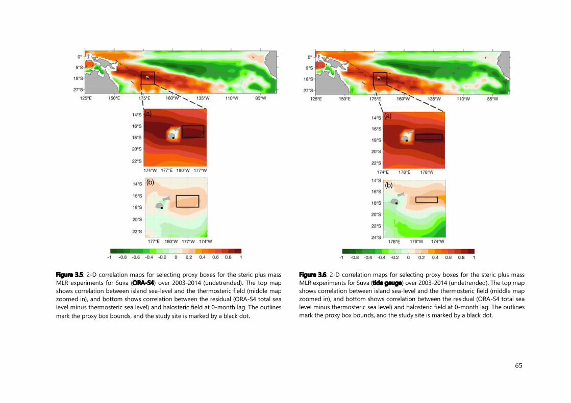
65

Figure 3.5: 2-D correlation maps for selecting proxy boxes for the steric plus mass MLR experiments for Suva (ORA-S4) over 2003-2014 (undetrended). The top map shows correlation between island sea-level and the thermosteric field (middle map zoomed in), and bottom shows correlation between the residual (ORA-S4 total sea level minus thermosteric sea level) and halosteric field at 0-month lag. The outlines mark the proxy box bounds, and the study site is marked by a black dot.

(b)

(a)

(b)

(a)

Figure 3.6: 2-D correlation maps for selecting proxy boxes for the steric plus mass MLR experiments for Suva (tide gauge) over 2003-2014 (undetrended). The top map shows correlation between island sea-level and the thermosteric field (middle map zoomed in), and bottom shows correlation between the residual (ORA-S4 total sea level minus thermosteric sea level) and halosteric field at 0-month lag. The outlines mark the proxy box bounds, and the study site is marked by a black dot.

66

Table 3.2: Proxy box bounds (longitude/latitude) for the thermosteric and halosteric regressors for the steric plus mass MLR experiments over 2003-2014.

3.6.2 Wind stress curl (Rossby wave model) dominated MLR models (1988-2014)

In this set of experiments, the first-order off equatorial and low frequency sea level response to wind stress curl at each site, i.e. the wind stress curl proxy, was taken as the resultant sea level anomaly from a linear Rossby wave model (Section 3.5; Kessler and Cravatte 2013a).

The residual of the thermosteric sea level variability from that induced by wind stress curl anomalies is due to buoyancy forcing at the air-sea surface and intrinsic ocean variability (Meyssignac et al. 2017). Thus, the other potential predictors include local SST to account for thermosteric sea level changes due to surface buoyancy forcing (Meyssignac et al. 2017), wind stress (τx, τy) in the vicinity of the island to represent the wind set-up, and halosteric sea level for salinity changes and surface freshwater fluxes (see Section 3.4.1).

In the first step to extract the regressor time series, spatial correlation maps between island sea level and wind stress curl-driven SLAs from the Rossby wave model were generated. As in the preliminary analysis (with steric and mass components, Section 3.6.1) proxy boxes were selected based on areas having highest correlation in the vicinity of the study site, as shown in Figures 3.7 -

Site Proxy box bounds (longitude, latitude)

Thermosteric Halosteric

ORA-S4 - detrended

Suva 180, 182, -18, -16 180, 184, -18, -16

Lautoka 173, 176, -16, -15 170, 175, -15, -13

Nouméa 168, 172, -22, -20 163, 167, -20, -17

ORA-S4 - undetrended

Suva 180, 184, -18, -16 181, 185, -18, -16

Lautoka 173, 177, -16, -15 170, 175, -15, -12

Nouméa 168, 172, -22, -20 163, 167, -20, -17

Tide gauge - detrended

Suva 180, 184, -18, -16 182, 185, -18, -16

Lautoka 180, 184, -18, -16 171, 174, -15, -13

Nouméa 167, 169, -22, -19 164, 166, -19, -17

Tide gauge - undetrended

Suva 180, 185, -18, -17 182, 186, -18, -17

Lautoka 180, 184, -18, -17 172, 175, -16, -15

Nouméa 168, 172, -21, -20 164, 167, -19, -17

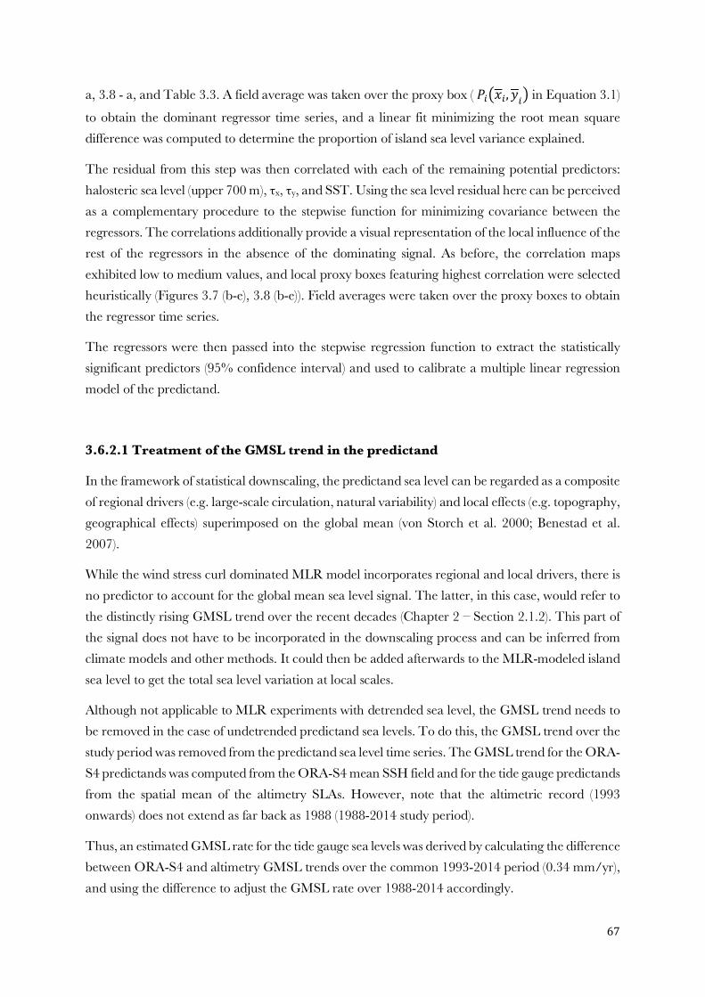
67

a, 3.8 - a, and Table 3.3. A field average was taken over the proxy box ( !"#$", &"' in Equation 3.1)

to obtain the dominant regressor time series, and a linear fit minimizing the root mean square difference was computed to determine the proportion of island sea level variance explained.

The residual from this step was then correlated with each of the remaining potential predictors: halosteric sea level (upper 700 m), τx, τy, and SST. Using the sea level residual here can be perceived as a complementary procedure to the stepwise function for minimizing covariance between the regressors. The correlations additionally provide a visual representation of the local influence of the rest of the regressors in the absence of the dominating signal. As before, the correlation maps exhibited low to medium values, and local proxy boxes featuring highest correlation were selected heuristically (Figures 3.7 (b-e), 3.8 (b-e)). Field averages were taken over the proxy boxes to obtain the regressor time series.

The regressors were then passed into the stepwise regression function to extract the statistically significant predictors (95% confidence interval) and used to calibrate a multiple linear regression model of the predictand.

3.6.2.1 Treatment of the GMSL trend in the predictand

In the framework of statistical downscaling, the predictand sea level can be regarded as a composite of regional drivers (e.g. large-scale circulation, natural variability) and local effects (e.g. topography, geographical effects) superimposed on the global mean (von Storch et al. 2000; Benestad et al. 2007).

While the wind stress curl dominated MLR model incorporates regional and local drivers, there is no predictor to account for the global mean sea level signal. The latter, in this case, would refer to the distinctly rising GMSL trend over the recent decades (Chapter 2 – Section 2.1.2). This part of the signal does not have to be incorporated in the downscaling process and can be inferred from climate models and other methods. It could then be added afterwards to the MLR-modeled island sea level to get the total sea level variation at local scales.

Although not applicable to MLR experiments with detrended sea level, the GMSL trend needs to be removed in the case of undetrended predictand sea levels. To do this, the GMSL trend over the study period was removed from the predictand sea level time series. The GMSL trend for the ORA-S4 predictands was computed from the ORA-S4 mean SSH field and for the tide gauge predictands from the spatial mean of the altimetry SLAs. However, note that the altimetric record (1993 onwards) does not extend as far back as 1988 (1988-2014 study period).

Thus, an estimated GMSL rate for the tide gauge sea levels was derived by calculating the difference between ORA-S4 and altimetry GMSL trends over the common 1993-2014 period (0.34 mm/yr), and using the difference to adjust the GMSL rate over 1988-2014 accordingly.

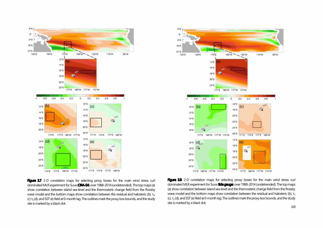
68

Figure 3.7: 2-D correlation maps for selecting proxy boxes for the main wind stress curl dominated MLR experiment for Suva (ORA-S4) over 1988-2014 (undetrended). The top maps (a) show correlation between island sea-level and the thermosteric change field from the Rossby wave model and the bottom maps show correlation between the residual and halosteric (b), τx, (c) τy (d), and SST (e) field at 0-month lag. The outlines mark the proxy box bounds, and the study site is marked by a black dot.

Figure 3.8: 2-D correlation maps for selecting proxy boxes for the main wind stress curl dominated MLR experiment for Suva (tide gauge) over 1988-2014 (undetrended). The top maps (a) show correlation between island sea-level and the thermosteric change field from the Rossby wave model and the bottom maps show correlation between the residual and halosteric (b), τx (c), τy (d), and SST (e) field at 0-month lag. The outlines mark the proxy box bounds, and the study site is marked by a black dot.

(a)

(b) (c)

(d) (e) (d)

(c)

(e)

(b)

(a)

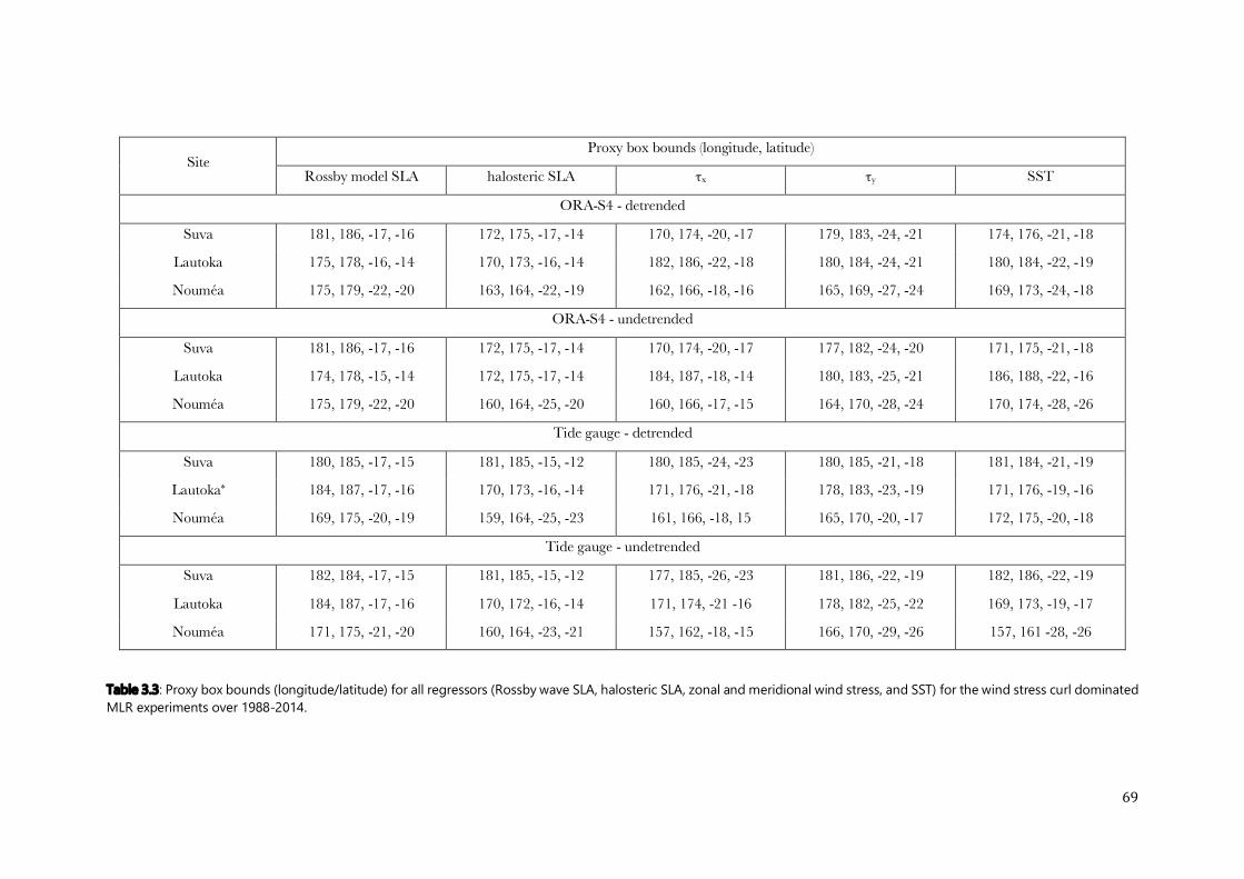
69


Rossby model SLA halosteric SLA τx τy SST

ORA-S4 - detrended

Suva 181, 186, -17, -16 172, 175, -17, -14 170, 174, -20, -17 179, 183, -24, -21 174, 176, -21, -18

Lautoka 175, 178, -16, -14 170, 173, -16, -14 182, 186, -22, -18 180, 184, -24, -21 180, 184, -22, -19

Nouméa 175, 179, -22, -20 163, 164, -22, -19 162, 166, -18, -16 165, 169, -27, -24 169, 173, -24, -18


Suva 181, 186, -17, -16 172, 175, -17, -14 170, 174, -20, -17 177, 182, -24, -20 171, 175, -21, -18

Lautoka 174, 178, -15, -14 172, 175, -17, -14 184, 187, -18, -14 180, 183, -25, -21 186, 188, -22, -16

Nouméa 175, 179, -22, -20 160, 164, -25, -20 160, 166, -17, -15 164, 170, -28, -24 170, 174, -28, -26


Suva 180, 185, -17, -15 181, 185, -15, -12 180, 185, -24, -23 180, 185, -21, -18 181, 184, -21, -19

Lautoka* 184, 187, -17, -16 170, 173, -16, -14 171, 176, -21, -18 178, 183, -23, -19 171, 176, -19, -16

Nouméa 169, 175, -20, -19 159, 164, -25, -23 161, 166, -18, 15 165, 170, -20, -17 172, 175, -20, -18


Suva 182, 184, -17, -15 181, 185, -15, -12 177, 185, -26, -23 181, 186, -22, -19 182, 186, -22, -19

Lautoka 184, 187, -17, -16 170, 172, -16, -14 171, 174, -21 -16 178, 182, -25, -22 169, 173, -19, -17

Nouméa 171, 175, -21, -20 160, 164, -23, -21 157, 162, -18, -15 166, 170, -29, -26 157, 161 -28, -26

Table 3.3: Proxy box bounds (longitude/latitude) for all regressors (Rossby wave SLA, halosteric SLA, zonal and meridional wind stress, and SST) for the wind stress curl dominated MLR experiments over 1988-2014.

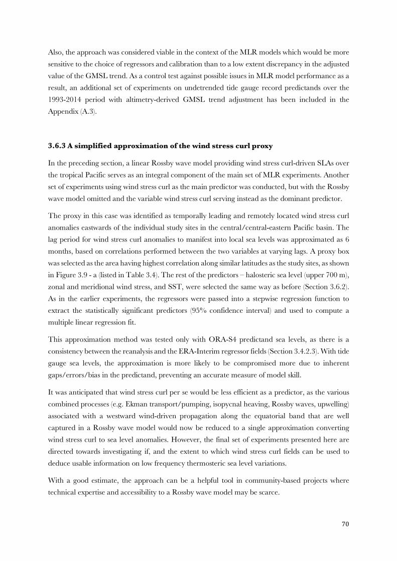
70

Also, the approach was considered viable in the context of the MLR models which would be more sensitive to the choice of regressors and calibration than to a low extent discrepancy in the adjusted value of the GMSL trend. As a control test against possible issues in MLR model performance as a result, an additional set of experiments on undetrended tide gauge record predictands over the 1993-2014 period with altimetry-derived GMSL trend adjustment has been included in the Appendix (A.3).

3.6.3 A simplified approximation of the wind stress curl proxy

In the preceding section, a linear Rossby wave model providing wind stress curl-driven SLAs over the tropical Pacific serves as an integral component of the main set of MLR experiments. Another set of experiments using wind stress curl as the main predictor was conducted, but with the Rossby wave model omitted and the variable wind stress curl serving instead as the dominant predictor.

The proxy in this case was identified as temporally leading and remotely located wind stress curl anomalies eastwards of the individual study sites in the central/central-eastern Pacific basin. The lag period for wind stress curl anomalies to manifest into local sea levels was approximated as 6 months, based on correlations performed between the two variables at varying lags. A proxy box was selected as the area having highest correlation along similar latitudes as the study sites, as shown in Figure 3.9 - a (listed in Table 3.4). The rest of the predictors – halosteric sea level (upper 700 m), zonal and meridional wind stress, and SST, were selected the same way as before (Section 3.6.2). As in the earlier experiments, the regressors were passed into a stepwise regression function to extract the statistically significant predictors (95% confidence interval) and used to compute a multiple linear regression fit.

This approximation method was tested only with ORA-S4 predictand sea levels, as there is a consistency between the reanalysis and the ERA-Interim regressor fields (Section 3.4.2.3). With tide gauge sea levels, the approximation is more likely to be compromised more due to inherent gaps/errors/bias in the predictand, preventing an accurate measure of model skill.

It was anticipated that wind stress curl per se would be less efficient as a predictor, as the various combined processes (e.g. Ekman transport/pumping, isopycnal heaving, Rossby waves, upwelling) associated with a westward wind-driven propagation along the equatorial band that are well captured in a Rossby wave model would now be reduced to a single approximation converting wind stress curl to sea level anomalies. However, the final set of experiments presented here are directed towards investigating if, and the extent to which wind stress curl fields can be used to deduce usable information on low frequency thermosteric sea level variations.

With a good estimate, the approach can be a helpful tool in community-based projects where technical expertise and accessibility to a Rossby wave model may be scarce.

71

Figure 3.9: 2-D correlation maps for selecting proxy boxes for the MLR experiment using the simplified approximation of the wind stress curl proxy for Suva (ORA-S4) over 1988-2014 (undetrended). The top maps (a) show correlation between island sea-level and the 6-month leading wind stress curl field and the bottom maps show correlation between the residual and halosteric (b), τx (c), τy (d), and SST (e) field at 0-month lag. The outlines mark the proxy box bounds, and the study site is marked by a black dot.

3.7 Stationarity test

The ultimate aim of developing a statistical downscaling model of this type is to be able to apply it to future projections of sea level and obtain information utilizable on local scales. Thus, the MLR models developed were tested for stationarity, i.e. could a model calibrated over one period be successfully applied to another period?

Since the study focuses on interannual-to-decadal scale variability, at least two decades of data were needed to successfully perform the stationarity test. Hence, the test only covers the main wind stress curl dominated (Section 3.6.2) and the simplified approximation method MLR experiments (Section 3.6.3). To conduct the test, an MLR model equation was calibrated over the first half (Aug 1988-Jul 2001) of the predictand dataset using the same set of predictors as the original model (i.e. stepwise regression excluded) and applied to the second half (Aug 2001 – Jul 2014).

(a)

(d) (e)

(c) (b)

72

Table 3.4: Proxy box bounds (longitude/latitude) for all regressors (wind stress curl, halosteric SLA, zonal and meridional wind stress, and SST) for the MLR experiments using the simplified approximation of the wind stress curl proxy over 1988-2014.


curlz τ halosteric SLA τx τy SST

ORA-S4 - detrended

Suva 204, 210, -18, -15 171, 176, -20, -17 170, 175, -18, -16 179, 182, -22, -17 179, 183, -24, -21

Lautoka 205, 213, -19, -16 170, 176, -21, -17 172, 175, -18, -17 180, 183, -22, -17 179, 183, -24, -21

Nouméa 181, 189, -23, -20 159, 162, -26, -24 160, 164, -16, -14 167, 170, -25, -21 169, 172, -26, -23


Suva 203, 208, -15, -18 171, 176, -21, -19 171, 174, -18, -16 179, 182, -22, -17 179, 183, -24, -21

Lautoka 205, 213, -19, -17 170, 176, -21, -19 172, 175, -19, -16 179, 182, -22, -17 178, 183, -24, -21

Nouméa 181, 189, -23, -20 159, 162, -26, -24 160, 166, -16, -14 168, 173, -24, -21 167, 174, -26, -23

73

The simulated sea level time series was compared to the predictand and to the original MLR modeled time series over the common period (second half). The test was also repeated in the opposite direction, i.e. computing an MLR model fit over the second half of the predictand dataset (Aug 2001 – Jul 2014) and applying it over the first half (Aug 1988-Jul 2001).

3.8 Summary

The thesis methodology is based on expressing island sea level variations at the study sites as a multiple linear regression of selected atmospheric and oceanic variables. The study period was 1988 to 2014, with a focus on interannual-to-decadal sea level variability and trend over this time. A stepwise regression function allowing the selection of statistically significant regressors was an integral part of the MLR model construction.

The predictand sea levels were taken from both the ORA-S4 reanalysis and tide gauge records, and predictor datasets were taken from GRACE (ocean mass), ERA-Interim atmospheric reanalysis, and ORA-S4 ocean reanalysis. In the preliminary set of MLR experiments conducted over a shorter 2003-2014 period (limited duration of ocean mass data), sea levels were first modeled as a sum of the thermosteric, halosteric, and mass components. A more dynamical approach was then undertaken, whereby wind stress curl was taken as a proxy for the dominant thermosteric component of sea level, and the rest of the regressors represented local effects. A Rossby wave model was employed to model the low-frequency thermosteric response of the tropical ocean to wind stress curl anomalies. In this main set of MLR experiments, the wind-forced thermosteric sea level change represented the leading regional regressor, while the minor, local regressors were represented by the halosteric component, wind stress vectors, and SSTs for freshwater fluxes, wind set-up, and surface heat fluxes respectively. Selection of the proxy boxes for the regressor time series was based on correlation maps and a stepwise regression function was used to isolate the final set of statistically significant regressors for the MLR model. An additional set of simplified, approximation method MLR experiments were also tested using the dynamical approach, but with the Rossby wave model omitted.

Finally, a stationarity test was employed to assess the MLR model’s applicability to future projections of island sea level, whereby the model’s performance was tested over periods other than which it had been calibrated over.

75

Chapter 4

Evaluation of ORA-S4 steric fields – a site adapted approach 4.1 Evaluation of ORA-S4 steric sea levels against a reanalyses ensemble ........ 77

4.2 Steric sea level depth – Upper 700 m vs. the deeper ocean ......................... 82

4.3 Covariance between the thermosteric and halosteric sea levels ................. 86

4.4 Summary ........................................................................................... 88

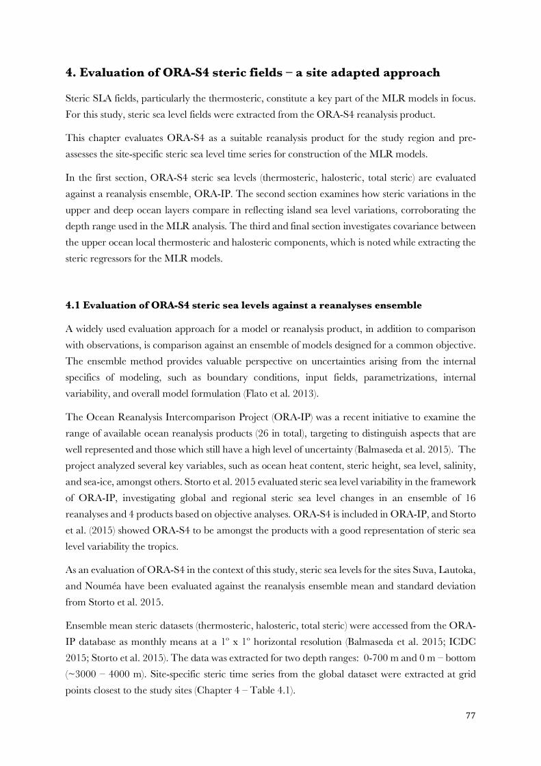
77

4. Evaluation of ORA-S4 steric fields – a site adapted approach

Steric SLA fields, particularly the thermosteric, constitute a key part of the MLR models in focus. For this study, steric sea level fields were extracted from the ORA-S4 reanalysis product.

This chapter evaluates ORA-S4 as a suitable reanalysis product for the study region and pre-assesses the site-specific steric sea level time series for construction of the MLR models.

In the first section, ORA-S4 steric sea levels (thermosteric, halosteric, total steric) are evaluated against a reanalysis ensemble, ORA-IP. The second section examines how steric variations in the upper and deep ocean layers compare in reflecting island sea level variations, corroborating the depth range used in the MLR analysis. The third and final section investigates covariance between the upper ocean local thermosteric and halosteric components, which is noted while extracting the steric regressors for the MLR models.

4.1 Evaluation of ORA-S4 steric sea levels against a reanalyses ensemble

A widely used evaluation approach for a model or reanalysis product, in addition to comparison with observations, is comparison against an ensemble of models designed for a common objective. The ensemble method provides valuable perspective on uncertainties arising from the internal specifics of modeling, such as boundary conditions, input fields, parametrizations, internal variability, and overall model formulation (Flato et al. 2013).

The Ocean Reanalysis Intercomparison Project (ORA-IP) was a recent initiative to examine the range of available ocean reanalysis products (26 in total), targeting to distinguish aspects that are well represented and those which still have a high level of uncertainty (Balmaseda et al. 2015). The project analyzed several key variables, such as ocean heat content, steric height, sea level, salinity, and sea-ice, amongst others. Storto et al. 2015 evaluated steric sea level variability in the framework of ORA-IP, investigating global and regional steric sea level changes in an ensemble of 16 reanalyses and 4 products based on objective analyses. ORA-S4 is included in ORA-IP, and Storto et al. (2015) showed ORA-S4 to be amongst the products with a good representation of steric sea level variability the tropics.

As an evaluation of ORA-S4 in the context of this study, steric sea levels for the sites Suva, Lautoka, and Nouméa have been evaluated against the reanalysis ensemble mean and standard deviation from Storto et al. 2015.

Ensemble mean steric datasets (thermosteric, halosteric, total steric) were accessed from the ORA-IP database as monthly means at a 1º x 1º horizontal resolution (Balmaseda et al. 2015; ICDC 2015; Storto et al. 2015). The data was extracted for two depth ranges: 0-700 m and 0 m – bottom (~3000 – 4000 m). Site-specific steric time series from the global dataset were extracted at grid points closest to the study sites (Chapter 4 – Table 4.1).

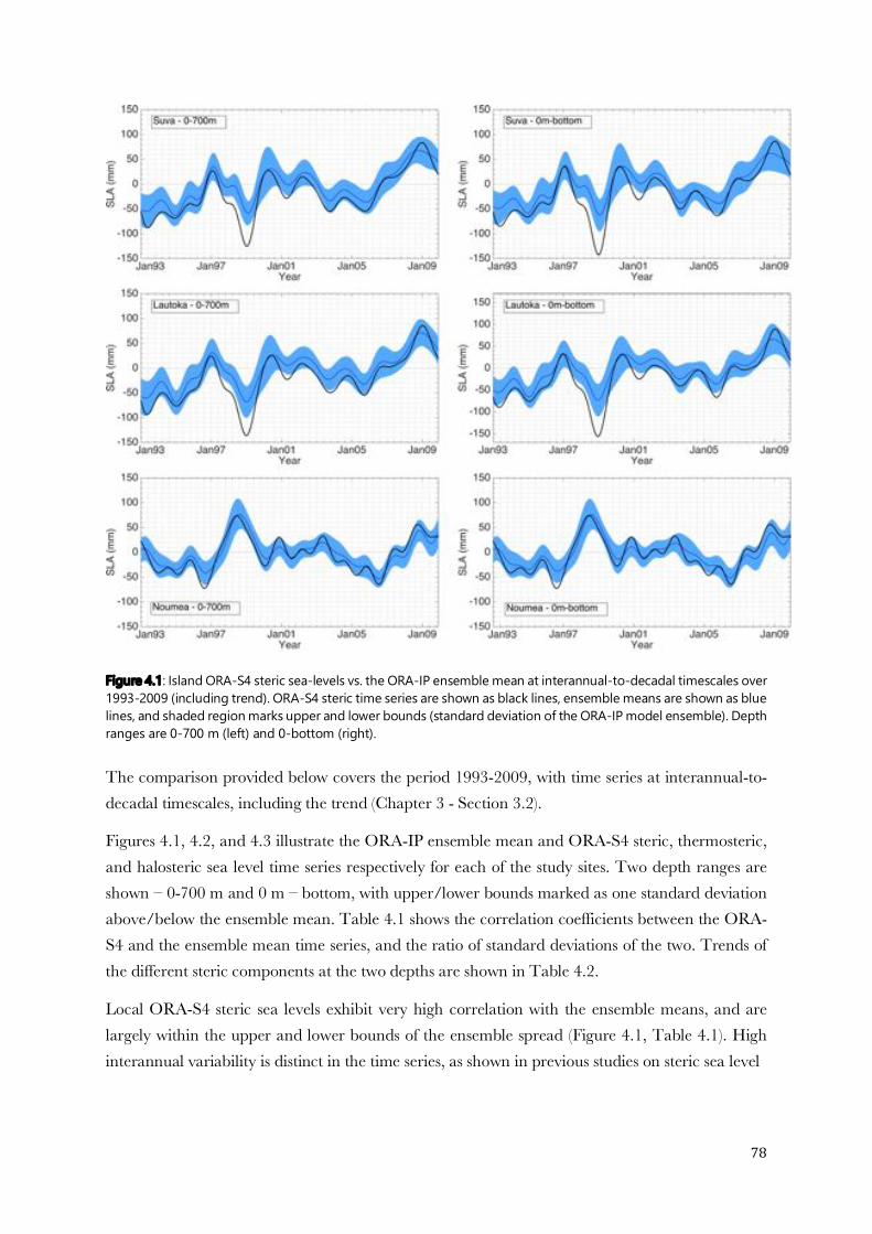
78

Figure 4.1: Island ORA-S4 steric sea-levels vs. the ORA-IP ensemble mean at interannual-to-decadal timescales over 1993-2009 (including trend). ORA-S4 steric time series are shown as black lines, ensemble means are shown as blue lines, and shaded region marks upper and lower bounds (standard deviation of the ORA-IP model ensemble). Depth ranges are 0-700 m (left) and 0-bottom (right). The comparison provided below covers the period 1993-2009, with time series at interannual-to-decadal timescales, including the trend (Chapter 3 - Section 3.2).

Figures 4.1, 4.2, and 4.3 illustrate the ORA-IP ensemble mean and ORA-S4 steric, thermosteric, and halosteric sea level time series respectively for each of the study sites. Two depth ranges are shown – 0-700 m and 0 m – bottom, with upper/lower bounds marked as one standard deviation above/below the ensemble mean. Table 4.1 shows the correlation coefficients between the ORA-S4 and the ensemble mean time series, and the ratio of standard deviations of the two. Trends of the different steric components at the two depths are shown in Table 4.2.

Local ORA-S4 steric sea levels exhibit very high correlation with the ensemble means, and are largely within the upper and lower bounds of the ensemble spread (Figure 4.1, Table 4.1). High interannual variability is distinct in the time series, as shown in previous studies on steric sea level

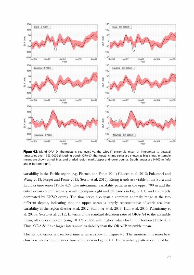
79

Figure 4.2: Island ORA-S4 thermosteric sea-levels vs. the ORA-IP ensemble mean at interannual-to-decadal timescales over 1993-2009 (including trend). ORA-S4 thermosteric time series are shown as black lines, ensemble means are shown as red lines, and shaded region marks upper and lower bounds. Depth ranges are 0-700 m (left) and 0-bottom (right). variability in the Pacific region (e.g. Piecuch and Ponte 2011; Church et al. 2013; Fukumori and Wang 2013; Forget and Ponte 2015; Storto et al. 2015). Rising trends are visible in the Suva and Lautoka time series (Table 4.2). The interannual variability patterns in the upper 700 m and the entire ocean column are very similar (compare right and left panels in Figure 4.1), and are largely dominated by ENSO events. The time series also span a common anomaly range at the two different depths, indicating that the upper ocean is largely representative of steric sea level variability in the region (Becker et al. 2012; Stammer et al. 2013; Han et al. 2014; Palanisamy et al. 2015a; Storto et al. 2015). In terms of the standard deviation ratio of ORA- S4 to the ensemble mean, all values exceed 1 (range = 1.21-1.43), with higher values for 0 m – bottom (Table 4.1). Thus, ORA-S4 has a larger interannual variability than the ORA-IP ensemble mean.

The island thermosteric sea level time series are shown in Figure 4.2. Thermosteric time series bear close resemblance to the steric time series seen in Figure 4.1. The variability pattern exhibited by

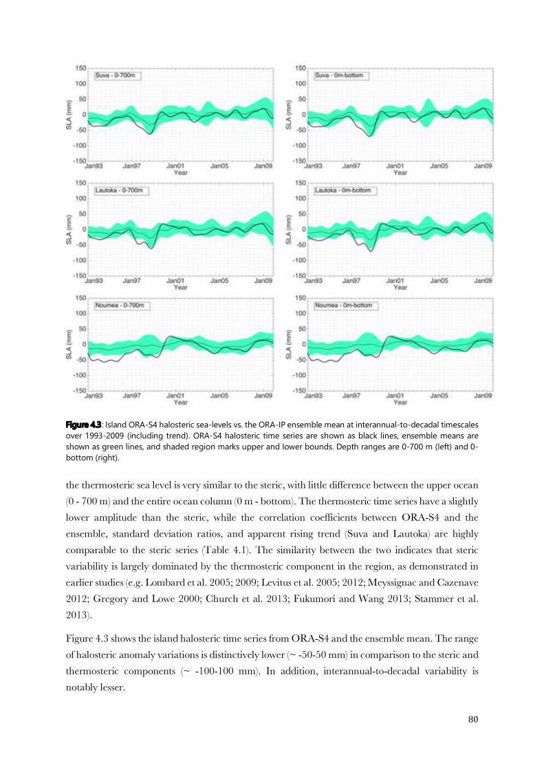
80

Figure 4.3: Island ORA-S4 halosteric sea-levels vs. the ORA-IP ensemble mean at interannual-to-decadal timescales over 1993-2009 (including trend). ORA-S4 halosteric time series are shown as black lines, ensemble means are shown as green lines, and shaded region marks upper and lower bounds. Depth ranges are 0-700 m (left) and 0-bottom (right). the thermosteric sea level is very similar to the steric, with little difference between the upper ocean (0 - 700 m) and the entire ocean column (0 m - bottom). The thermosteric time series have a slightly lower amplitude than the steric, while the correlation coefficients between ORA-S4 and the ensemble, standard deviation ratios, and apparent rising trend (Suva and Lautoka) are highly comparable to the steric series (Table 4.1). The similarity between the two indicates that steric variability is largely dominated by the thermosteric component in the region, as demonstrated in earlier studies (e.g. Lombard et al. 2005; 2009; Levitus et al. 2005; 2012; Meyssignac and Cazenave 2012; Gregory and Lowe 2000; Church et al. 2013; Fukumori and Wang 2013; Stammer et al. 2013).

Figure 4.3 shows the island halosteric time series from ORA-S4 and the ensemble mean. The range of halosteric anomaly variations is distinctively lower (~ -50-50 mm) in comparison to the steric and thermosteric components (~ -100-100 mm). In addition, interannual-to-decadal variability is notably lesser.

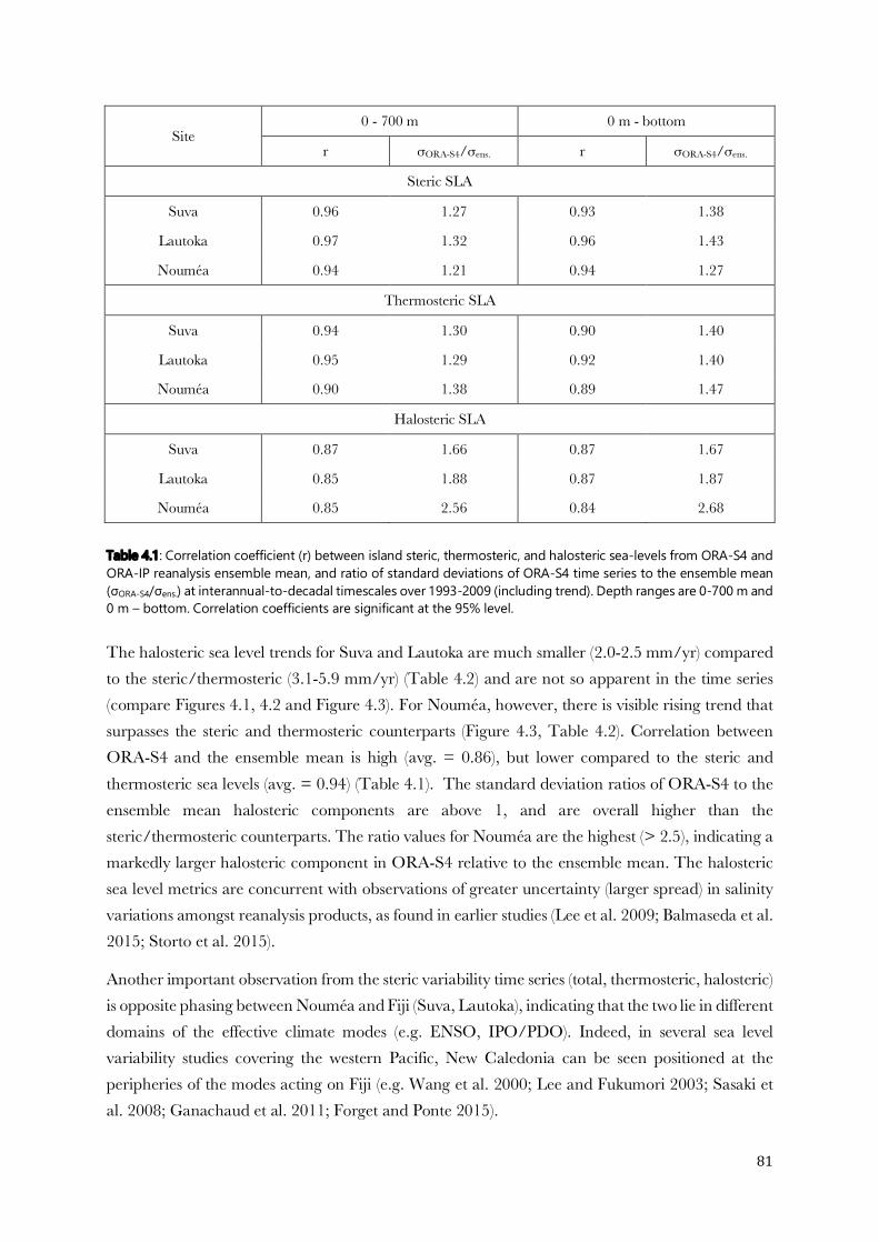
81

Site 0 - 700 m 0 m - bottom

r σORA-S4/σens. r σORA-S4/σens.

Steric SLA

Suva 0.96 1.27 0.93 1.38

Lautoka 0.97 1.32 0.96 1.43

Nouméa 0.94 1.21 0.94 1.27

Thermosteric SLA

Suva 0.94 1.30 0.90 1.40

Lautoka 0.95 1.29 0.92 1.40

Nouméa 0.90 1.38 0.89 1.47

Halosteric SLA

Suva 0.87 1.66 0.87 1.67

Lautoka 0.85 1.88 0.87 1.87

Nouméa 0.85 2.56 0.84 2.68

Table 4.1: Correlation coefficient (r) between island steric, thermosteric, and halosteric sea-levels from ORA-S4 and ORA-IP reanalysis ensemble mean, and ratio of standard deviations of ORA-S4 time series to the ensemble mean (σORA-S4/σens.) at interannual-to-decadal timescales over 1993-2009 (including trend). Depth ranges are 0-700 m and 0 m – bottom. Correlation coefficients are significant at the 95% level. The halosteric sea level trends for Suva and Lautoka are much smaller (2.0-2.5 mm/yr) compared to the steric/thermosteric (3.1-5.9 mm/yr) (Table 4.2) and are not so apparent in the time series (compare Figures 4.1, 4.2 and Figure 4.3). For Nouméa, however, there is visible rising trend that surpasses the steric and thermosteric counterparts (Figure 4.3, Table 4.2). Correlation between ORA-S4 and the ensemble mean is high (avg. = 0.86), but lower compared to the steric and thermosteric sea levels (avg. = 0.94) (Table 4.1). The standard deviation ratios of ORA-S4 to the ensemble mean halosteric components are above 1, and are overall higher than the steric/thermosteric counterparts. The ratio values for Nouméa are the highest (> 2.5), indicating a markedly larger halosteric component in ORA-S4 relative to the ensemble mean. The halosteric sea level metrics are concurrent with observations of greater uncertainty (larger spread) in salinity variations amongst reanalysis products, as found in earlier studies (Lee et al. 2009; Balmaseda et al. 2015; Storto et al. 2015).

Another important observation from the steric variability time series (total, thermosteric, halosteric) is opposite phasing between Nouméa and Fiji (Suva, Lautoka), indicating that the two lie in different domains of the effective climate modes (e.g. ENSO, IPO/PDO). Indeed, in several sea level variability studies covering the western Pacific, New Caledonia can be seen positioned at the peripheries of the modes acting on Fiji (e.g. Wang et al. 2000; Lee and Fukumori 2003; Sasaki et al. 2008; Ganachaud et al. 2011; Forget and Ponte 2015).

82

Site

Trend (mm/yr)

0 – 700 m 0 m - bottom

ensemble mean ORA-S4 ensemble mean ORA-S4

Steric SLA

Suva 4.5 ± 0.2 5.6 ± 0.3 3.8 ± 0.2 5.3 ± 0.3

Lautoka 4.7 ± 0.2 5.9 ± 0.3 4.1 ± 0.2 5.6 ± 0.3

Nouméa 0.6 ± 0.03 1.7 ± 0.1 0.5 ± 0.03 1.7 ± 0.1

Thermosteric SLA

Suva 2.9 ± 0.1 3.1 ± 0.2 2.2 ± 0.1 2.7 ± 0.1

Lautoka 3.4 ± 0.2 3.9 ± 0.2 2.8 ± 0.1 3.3 ± 0.2

Nouméa -0.6 ± 0.03 -1.7 ± 0.1 -0.8 ± 0.04 -1.7 ± 0.1

Halosteric SLA

Suva 1.6 ± 0.1 2.5 ± 0.1 1.6 ± 0.1 2.7 ± 0.1

Lautoka 1.3 ± 0.1 2.0 ± 0.1 1.4 ± 0.1 2.4 ± 0.1

Nouméa 1.2 ± 0.1 3.1 ± 0.2 1.3 ± 0.1 3.1 ± 0.2

Table 4.2: Trends of island steric, thermosteric, and halosteric sea-levels from ORA-S4 and ORA-IP reanalysis ensemble mean over 1993-2009. Note that the uncertainty values are not the standard deviations, but the formal error of the trend computation. Depth ranges are 0-700 m and 0 m – bottom. In summary, the steric sea level time series shown in Figure 4.1 can be perceived as a composite of the thermosteric and halosteric components (Figures 4.2, 4.3), dominated by the former in the region. Interannual-to-decadal steric sea level variability (total, thermosteric, halosteric) in ORA-S4 has high correlation with the ensemble mean, exhibiting robustness in the reanalysis product. While the amplitude of variability is generally higher in ORA-S4 with respect to the ensemble mean, it is still largely within the ensemble spread. Such discrepancies are more pronounced with the halosteric sea level, where the inter-reanalyses spreads are the highest.

4.2 Steric sea level depth – Upper 700 m vs. the deeper ocean

Regional sea level variations essentially reflect those of the upper ocean. The Pacific Ocean steric sea level is modulated largely by natural internal variability on interannual-to-decadal/multi-decadal timescales, which influences the thermal structure of the upper oceans in most regions (Wang et al. 2000; Qiu and Chen 2006; Timmerman et al. 2010; McGregor et al. 2012; Forget and Ponte 2015; Nieves et al. 2017). While the upper ocean has dominated ocean heat uptake over the recent decades, there are observations of warming extending into the deeper oceans as well (Johnson et al. 2007; Domingues et al. 2008; Lyman et al. 2010; Church et al. 2013, Durack et al. 2014; 2018).

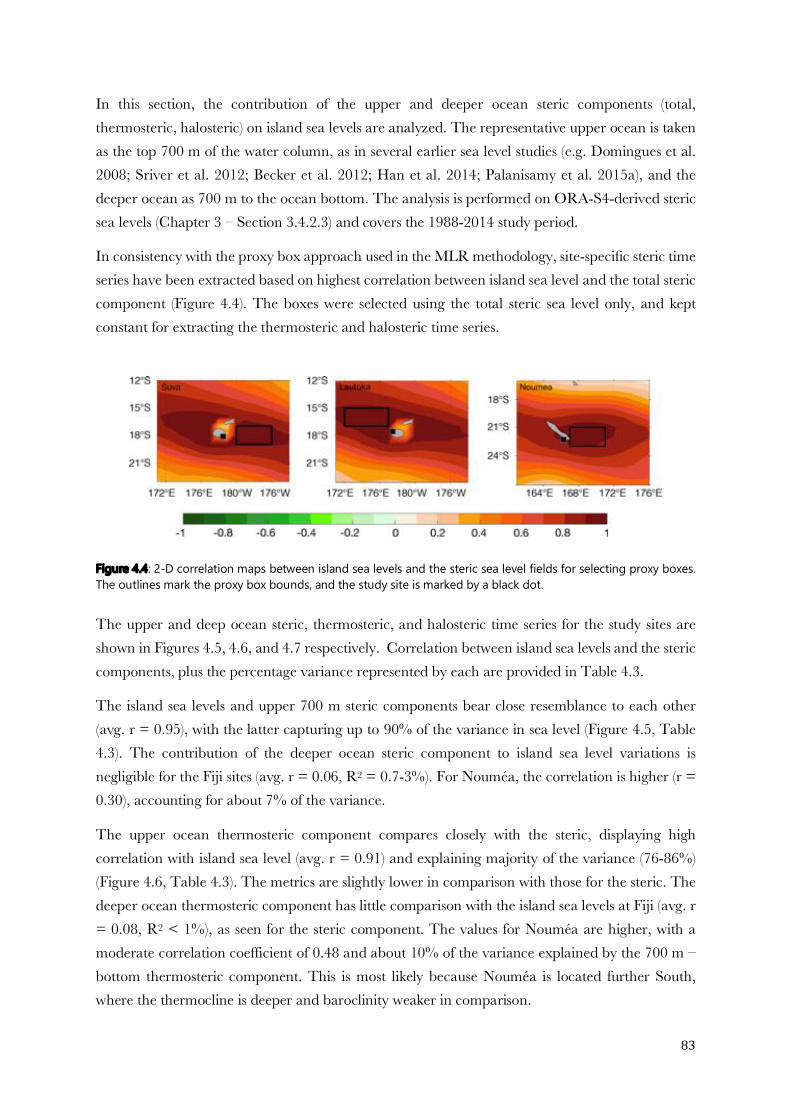
83

In this section, the contribution of the upper and deeper ocean steric components (total, thermosteric, halosteric) on island sea levels are analyzed. The representative upper ocean is taken as the top 700 m of the water column, as in several earlier sea level studies (e.g. Domingues et al. 2008; Sriver et al. 2012; Becker et al. 2012; Han et al. 2014; Palanisamy et al. 2015a), and the deeper ocean as 700 m to the ocean bottom. The analysis is performed on ORA-S4-derived steric sea levels (Chapter 3 – Section 3.4.2.3) and covers the 1988-2014 study period.

In consistency with the proxy box approach used in the MLR methodology, site-specific steric time series have been extracted based on highest correlation between island sea level and the total steric component (Figure 4.4). The boxes were selected using the total steric sea level only, and kept constant for extracting the thermosteric and halosteric time series.

Figure 4.4: 2-D correlation maps between island sea levels and the steric sea level fields for selecting proxy boxes. The outlines mark the proxy box bounds, and the study site is marked by a black dot. The upper and deep ocean steric, thermosteric, and halosteric time series for the study sites are shown in Figures 4.5, 4.6, and 4.7 respectively. Correlation between island sea levels and the steric components, plus the percentage variance represented by each are provided in Table 4.3.

The island sea levels and upper 700 m steric components bear close resemblance to each other (avg. r = 0.95), with the latter capturing up to 90% of the variance in sea level (Figure 4.5, Table 4.3). The contribution of the deeper ocean steric component to island sea level variations is negligible for the Fiji sites (avg. r = 0.06, R2 = 0.7-3%). For Nouméa, the correlation is higher (r = 0.30), accounting for about 7% of the variance.

The upper ocean thermosteric component compares closely with the steric, displaying high correlation with island sea level (avg. r = 0.91) and explaining majority of the variance (76-86%) (Figure 4.6, Table 4.3). The metrics are slightly lower in comparison with those for the steric. The deeper ocean thermosteric component has little comparison with the island sea levels at Fiji (avg. r = 0.08, R2 < 1%), as seen for the steric component. The values for Nouméa are higher, with a moderate correlation coefficient of 0.48 and about 10% of the variance explained by the 700 m – bottom thermosteric component. This is most likely because Nouméa is located further South, where the thermocline is deeper and baroclinity weaker in comparison.

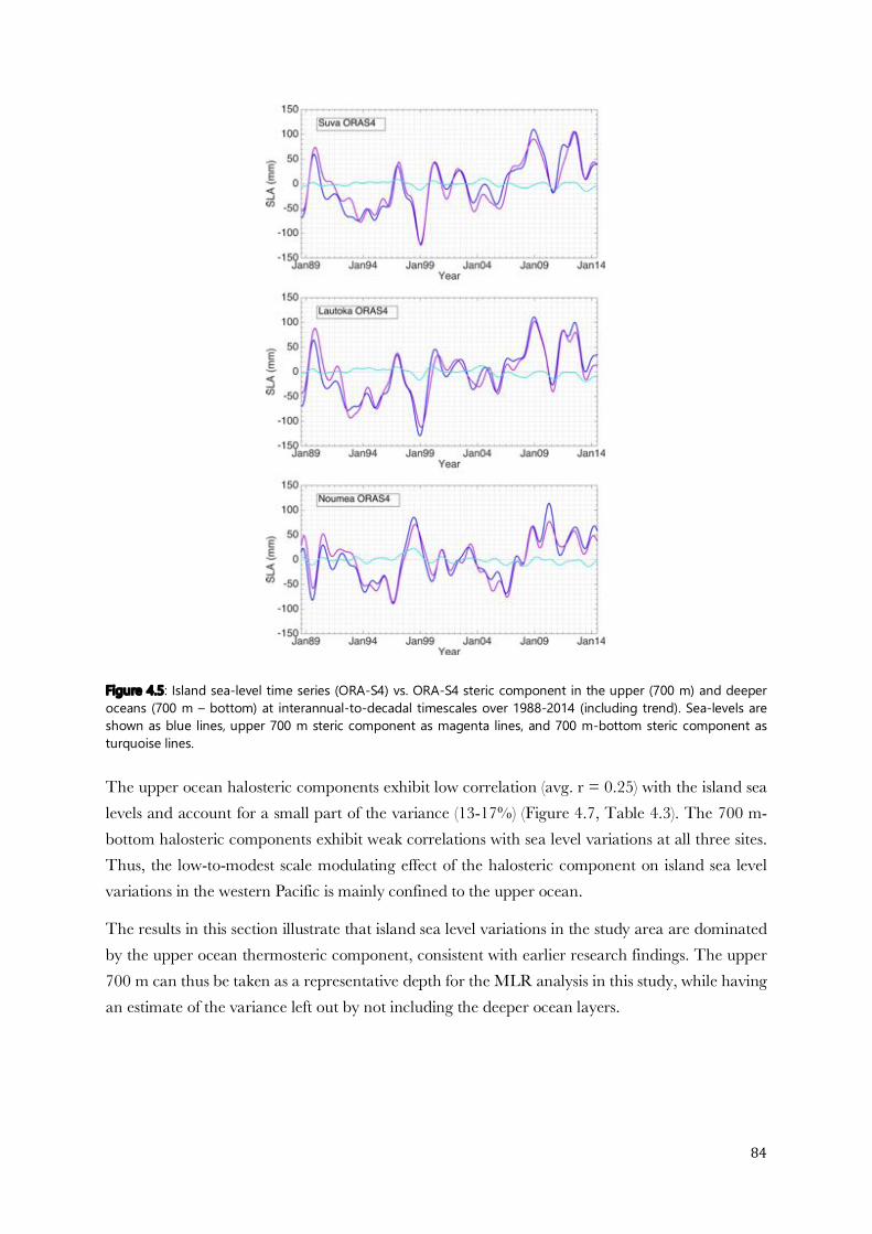
84

Figure 4.5: Island sea-level time series (ORA-S4) vs. ORA-S4 steric component in the upper (700 m) and deeper oceans (700 m – bottom) at interannual-to-decadal timescales over 1988-2014 (including trend). Sea-levels are shown as blue lines, upper 700 m steric component as magenta lines, and 700 m-bottom steric component as turquoise lines. The upper ocean halosteric components exhibit low correlation (avg. r = 0.25) with the island sea levels and account for a small part of the variance (13-17%) (Figure 4.7, Table 4.3). The 700 m-bottom halosteric components exhibit weak correlations with sea level variations at all three sites. Thus, the low-to-modest scale modulating effect of the halosteric component on island sea level variations in the western Pacific is mainly confined to the upper ocean.

The results in this section illustrate that island sea level variations in the study area are dominated by the upper ocean thermosteric component, consistent with earlier research findings. The upper 700 m can thus be taken as a representative depth for the MLR analysis in this study, while having an estimate of the variance left out by not including the deeper ocean layers.

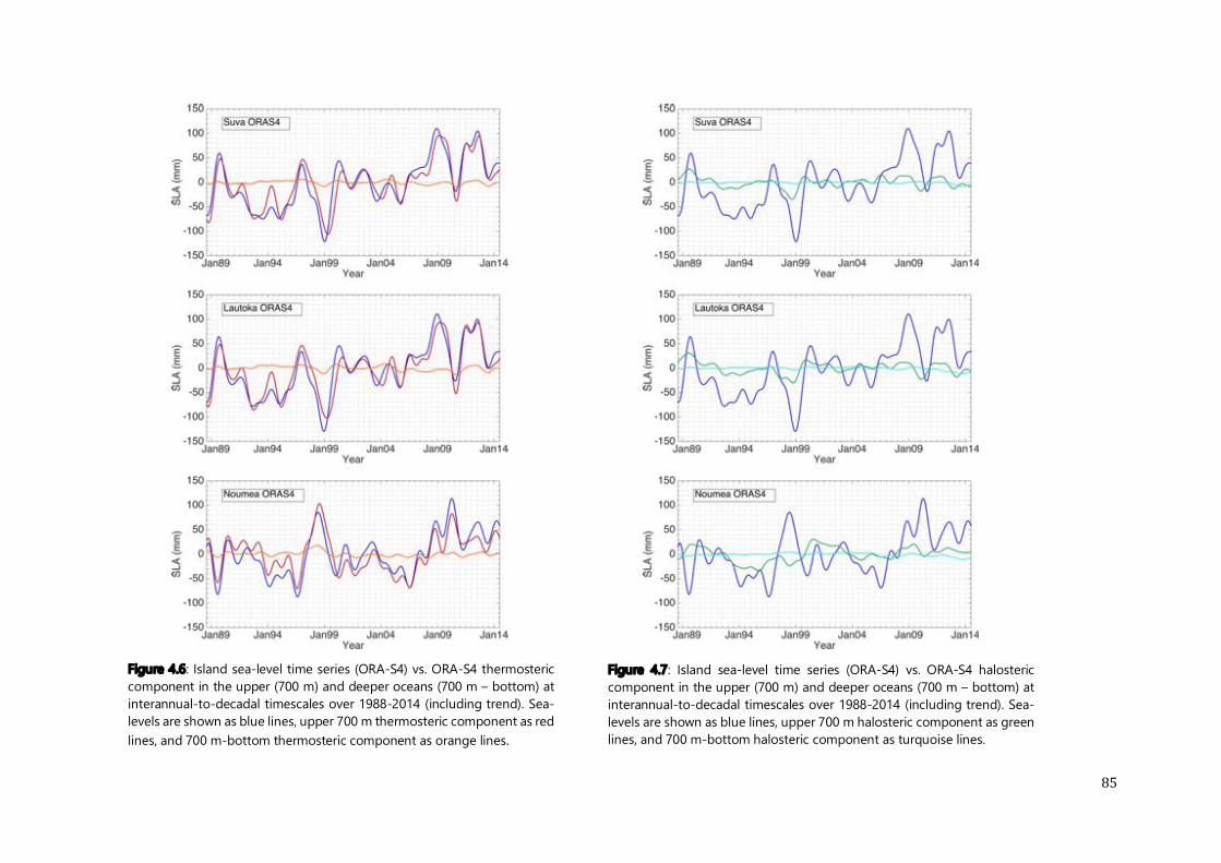
85

Figure 4.6: Island sea-level time series (ORA-S4) vs. ORA-S4 thermosteric component in the upper (700 m) and deeper oceans (700 m – bottom) at interannual-to-decadal timescales over 1988-2014 (including trend). Sea-levels are shown as blue lines, upper 700 m thermosteric component as red lines, and 700 m-bottom thermosteric component as orange lines.

Figure 4.7: Island sea-level time series (ORA-S4) vs. ORA-S4 halosteric component in the upper (700 m) and deeper oceans (700 m – bottom) at interannual-to-decadal timescales over 1988-2014 (including trend). Sea-levels are shown as blue lines, upper 700 m halosteric component as green lines, and 700 m-bottom halosteric component as turquoise lines.

86

Table 4.3: Correlation coefficient (r) between island sea-levels (ORA-S4) and ORA-S4 steric, thermosteric, and halosteric components in the upper (700 m) and deeper oceans (700 m – bottom), and percentage variance (R2) explained by each at interannual-to-decadal timescales over 1988-2014 (including trend). Correlation coefficients are significant at the 95% level.

4.3 Covariance between the thermosteric and halosteric sea levels

The thermosteric (or its proxy) and halosteric sea levels are key predictors in the MLR models for island sea levels. The behavior of the thermosteric and halosteric components in relation to each other is governed largely by isopycnal motion, mixed layer contributions, and ocean spiciness, with the halosteric component compensating the thermosteric in some regions (Levitus et al. 2005; Ishii et al. 2006; Köhl 2014; Forget and Ponte 2015; Meyssignac et al. 2017). Being affected by the same climate modes on interannual-to-decadal timescales, the two may share correlating patterns to some extent. In this section, the degree of correlation between the upper 700 m thermosteric and halosteric components introduced in the preceding section is investigated over the 1988-2014 study period.

Figure 4.8 shows the thermosteric and halosteric component time series for the study sites. Correlation coefficients between the two are provided in Table 4.4.

The halosteric sea levels exhibit little variation on interannual timescales, and apart from some lagged similarities during pronounced variability in the thermosteric component corresponding to notable ENSO events (e.g.1988-99, 2009-10, 2011-12), no consistent relationship is apparent between the two (Figure 4.8). The correlation coefficients between the two components are low (≈ 0.3).

Site 0 - 700 m 700 m - bottom

r R2 (%) r R2 (%)

Steric SLA

Suva 0.95 90.0 0.08 0.7

Lautoka 0.95 89.7 0.03 2.9

Nouméa 0.94 87.4 0.30 7.1

Thermosteric SLA

Suva 0.92 84.5 0.09 0.8

Lautoka 0.93 86.0 0.06 0.2

Nouméa 0.87 76.0 0.48 9.7

Halosteric SLA

Suva 0.24 14.5 0.05 0.2

Lautoka 0.28 17.1 0.15 2.4

Nouméa 0.22 13.3 0.10 2.0

87

Figure 4.8: Time series of island thermosteric and halosteric sea-levels in the upper 700 m at interannual-to-decadal timescales over 1988-2014 (including trend). The thermosteric component is shown as red lines, halosteric component as green lines, and the local sea-level as dotted blue lines.

Site r

Suva 0.26

Lautoka 0.29

Nouméa 0.31

Table 4.4: Correlation coefficient (r) between the thermosteric and halosteric sea-levels in the upper 700 m at interannual-to-decadal timescales over 1988-2014 (including trend). Correlation coefficients are significant at the 95% level. Note that for the MLR analysis, unlike in this section, the thermosteric and halosteric regressors are not extracted from the same proxy boxes – the variance represented by the dominant regressor is removed from the island sea level before selecting the halosteric predictor in attempts to minimize cross-correlations (Chapter 3 – Section 3.6). Thus, the correlation between the thermosteric and halosteric regressors used in the MLR models may be slightly different.

88

4.4 Summary

Based on comparisons with the ocean reanalyses ensemble, ORA-IP, steric sea levels from the ORA-S4 reanalysis have high agreement with the ensemble mean at the study sites. While the amplitude of steric sea level variability is generally higher in ORA-S4 relative to the ensemble mean, it remains largely within the ensemble spread. Discrepancies between ORA-S4 and the ensemble steric sea levels are more apparent in the halosteric component, where the inter-reanalyses spreads are the largest. The majority of steric sea level variations are confined to the upper ocean, thus the upper 700 m can be taken a representative depth for the MLR analysis (as in many other studies). Furthermore, while some degree of covariance can indeed be expected between the thermosteric and halosteric components, correlation between the two at the study sites is generally quite weak.

Overall, steric sea level variability at the study sites is dominated by the thermosteric component, and ORA-S4 is indeed a suitable reanalysis product for the MLR analysis.

89

Chapter 5

Results 5.1 Island sea level time series ...................................................................... 91

5.2 MLR results........................................................................................... 94 5.2.1 Preliminary steric plus mass MLR models (2003-2014) ....................................................94

5.2.1.1 Steric plus mass regressor time series .........................................................................94 5.2.1.2 Steric plus mass MLR models ....................................................................................99

5.2.2 Wind stress curl (Rossby wave model) dominated MLR models (1988-2014) ................103 5.2.3 Simplified approximation method MLRs (1988-2014) ...................................................111

5.3 Stationarity Test .................................................................................. 117

5.4 Summary ............................................................................................ 125

91

5. Results

This chapter presents the results of the MLR experiments described in Chapter 4. The MLR results have been published in an article in the Journal of Geophysical Research: Oceans and are transcribed hereafter with more details. The original article can be found in Annex 1.

The results chapter begins with sea level anomaly time series from in situ, altimetry, and reanalysis data for the study sites. Their trends are then analyzed and compared. The focus MLR results are presented next – preliminary steric plus mass MLR models, main wind stress curl-dominated models, and the simplified approximation method models. The models are evaluated via comparisons between the modeled and predictand sea level time series (correlations, percentage variance explained, trends). Equations of the calibrated MLR models are also analyzed to understand the roles of individual predictor variables and compared with existing knowledge to obtain insight into related model skills or limitations. The chapter concludes with results of the stationarity test for the calibrated models.

Additional figures and tables supplementing the results provided here have been included in the Appendix, and made reference to where relevant.

5.1 Island sea level time series

Sea level time series for the study sites from tide gauges (1988-2014), altimetry (1993-2014), and ORA-S4 (1988-2014) on interannual timescales are shown in Figure 5.1 and trends provided in Table 5.1. Correlation coefficients between the different datasets over common periods are shown in Table 5.2.

The altimetry and ORA-S4 sea level time series have high correlation with each other (r = 0.93-0.96) and show very similar trends over the 1993-2014 period (Figure 5.1, Tables 5.1, 5.2). This is expected as the ORA-S4 reanalysis assimilates altimetric data (Chapter 3 - Section 3.4.2.3). The tide gauge time series are generally similar to altimetry and ORA-S4, but exhibit discrepancies at times as a result of vertical land motion described earlier in Chapter 3 – Section 3.3, and other possible bias (e.g. instrumental error) (Aucan et al. 2017; Mörner and Klein 2017). Inconsistencies are visible between the tide gauge sea levels and altimetry/ORA-S4 at Suva during 1988-94, 1997-99, and 2011 onwards, and at Nouméa during 1989-97; these are likely due to site specific subsidence or uplift, or relocation of the tide gauge (Aucan et al. 2017; Mörner and Klein 2017).

In terms of the study sites, Suva and Lautoka display rising trends, which are more pronounced over the 2nd half of the study period (Figure 5.1). Over both the 1988-2014 and 1993-2014 periods, the tide gauge trends for Suva (6.8 mm/yr, 8.5 mm/yr respectively; relative sea level) are notably higher than those in ORA-S4 (4.1 mm/yr, 6.1 mm/yr) and altimetry (6.1 mm/yr) (absolute sea level), suggesting subsidence at the site.

92

Figure 5.1: Interannual sea-level time series at Suva (top panel), Lautoka (middle panel) and Nouméa (bottom panel) over the 1988-2014 period. Blue lines represent tide gauges, green lines represent ORA-S4, and magenta shows altimetry time series. The Lautoka tide gauge trend over the 1993-2014 period (5.5. mm/yr), which overlaps with Suva, matches ORA-S4 (5.8 mm/yr) and altimetry (5.5 mm/yr). However, the trend from the Suva tide gauge is much higher than that for Lautoka, and the difference (3 mm/yr) is beyond what would generally be expected from ocean dynamics given the proximity of the two sites. The anomalous trend from the Suva tide gauge is consistent with a high likelihood of sediment-compaction subsidence at the site, which results in a slow relative sea level rise over time (Mörner and Klein 2017).

While spanning a shorter period (1993-2014), the Lautoka tide gauge sea levels are highly consistent with ORA-S4 and altimetry (Tables 5.1, 5.2), demonstrating a record more reliable than Suva’s. Unlike the assertions in Mörner and Klein 2017, no strong indication of subsidence is visible at Lautoka from the current analysis; the relative and absolute sea level (altimetry) trends are the same

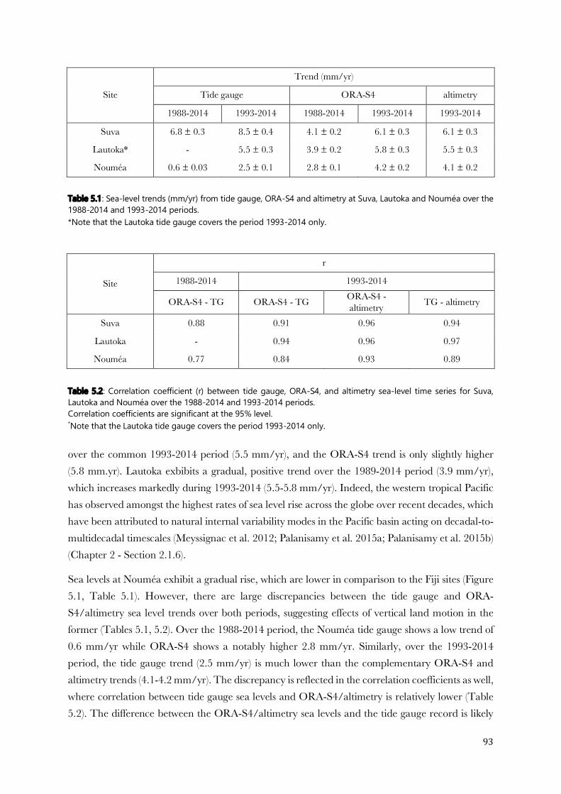
93

Site

Trend (mm/yr)

Tide gauge ORA-S4 altimetry

1988-2014 1993-2014 1988-2014 1993-2014 1993-2014

Suva 6.8 ± 0.3 8.5 ± 0.4 4.1 ± 0.2 6.1 ± 0.3 6.1 ± 0.3

Lautoka* - 5.5 ± 0.3 3.9 ± 0.2 5.8 ± 0.3 5.5 ± 0.3

Nouméa 0.6 ± 0.03 2.5 ± 0.1 2.8 ± 0.1 4.2 ± 0.2 4.1 ± 0.2

Table 5.1: Sea-level trends (mm/yr) from tide gauge, ORA-S4 and altimetry at Suva, Lautoka and Nouméa over the 1988-2014 and 1993-2014 periods. *Note that the Lautoka tide gauge covers the period 1993-2014 only.

Site

r

1988-2014 1993-2014

ORA-S4 - TG ORA-S4 - TG ORA-S4 - altimetry TG - altimetry

Suva 0.88 0.91 0.96 0.94

Lautoka - 0.94 0.96 0.97

Nouméa 0.77 0.84 0.93 0.89

Table 5.2: Correlation coefficient (r) between tide gauge, ORA-S4, and altimetry sea-level time series for Suva, Lautoka and Nouméa over the 1988-2014 and 1993-2014 periods. Correlation coefficients are significant at the 95% level. *Note that the Lautoka tide gauge covers the period 1993-2014 only. over the common 1993-2014 period (5.5 mm/yr), and the ORA-S4 trend is only slightly higher (5.8 mm.yr). Lautoka exbibits a gradual, positive trend over the 1989-2014 period (3.9 mm/yr), which increases markedly during 1993-2014 (5.5-5.8 mm/yr). Indeed, the western tropical Pacific has observed amongst the highest rates of sea level rise across the globe over recent decades, which have been attributed to natural internal variability modes in the Pacific basin acting on decadal-to-multidecadal timescales (Meyssignac et al. 2012; Palanisamy et al. 2015a; Palanisamy et al. 2015b) (Chapter 2 - Section 2.1.6).

Sea levels at Nouméa exhibit a gradual rise, which are lower in comparison to the Fiji sites (Figure 5.1, Table 5.1). However, there are large discrepancies between the tide gauge and ORA-S4/altimetry sea level trends over both periods, suggesting effects of vertical land motion in the former (Tables 5.1, 5.2). Over the 1988-2014 period, the Nouméa tide gauge shows a low trend of 0.6 mm/yr while ORA-S4 shows a notably higher 2.8 mm/yr. Similarly, over the 1993-2014 period, the tide gauge trend (2.5 mm/yr) is much lower than the complementary ORA-S4 and altimetry trends (4.1-4.2 mm/yr). The discrepancy is reflected in the correlation coefficients as well, where correlation between tide gauge sea levels and ORA-S4/altimetry is relatively lower (Table 5.2). The difference between the ORA-S4/altimetry sea levels and the tide gauge record is likely

94

due to uplift at the Nouméa site, resulting in a lower relative sea-level rise rate. Indeed, according to Aucan et al. 2017, who compiled the merged Nouméa tide gauge record, uplift rates of 1.3-1.4 mm/yr over most of the duration of the record can be inferred via comparisons with satellite altimetry and global sea-level reconstructions. Adjusting for vertical land motion based on these values would raise the tide gauge trend to ~3.9mm/yr, which is close to the trends from ORA-S4 and altimetry.

5.2 MLR results

Results for each of the MLR experiments are presented in the form of: (1) predictand and MLR modeled sea level time series, (2) correlation coefficient between the two and the percentage variance explained by modeled time series, (3) predictand and modeled sea level trends, and (4) MLR model equations.

For the preliminary set of MLR experiments, additional regressor time series, and correlation coefficients between the individual regressors and the predictand, plus percentage variance explained by each are shown to illustrate the predictor skills of the steric and mass components. The same metrics for the rest of the MLR experiments are provided in the Appendix.

In the article published in the Journal of Geophysical Research: Oceans based on this thesis (Annex 1), only MLR experiments conducted with ORA-S4 predictands are presented. In the following sections, the experiments performed with tide gauge predictands are included. Also, the simplified approximation method MLR experiments (Section 5.2.3) mentioned in the article are presented in detail. Similarly, while the stationarity test was shown for only one of the MLR experiments in the article, it is presented for all experiments covering the 1988-2014 period in Section 5.3.

5.2.1 Preliminary steric plus mass MLR models (2003-2014)

5.2.1.1 Steric plus mass regressor time series

The aim of this section is to illustrate the respective contributions of the steric and mass components to sea level variability before proceeding to the preliminary MLR results over the 2003-2014 period. Regressor time series, i.e. the thermosteric, halosteric and mass components that were linearly

regressed on the predictand (i.e. ∝" #"$%", '", ( − ("* from Chapter 3 – Equation 3.1), together with

the predictand time series (ORA-S4 and tide gauges) are shown in Figures 5.2 and 5.3 for the detrended and undetrended sets respectively.

Note that the linearly regressed steric time series shown here illustrate how the thermosteric and halosteric components are represented in the calibrated MLR model, hence they are not identical to those in the preceding chapter (Chapter 4 – Sections 4.2, 4.3).

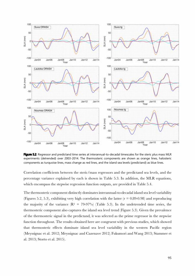
95

Figure 5.2: Regressor and predictand time series at interannual-to-decadal timescales for the steric plus mass MLR experiments (detrended) over 2003-2014. The thermosteric components are shown as orange lines, halosteric components as turquoise lines, mass change as red lines, and the island sea levels (predictand) as blue lines. Correlation coefficients between the steric/mass regressors and the predictand sea levels, and the percentage variance explained by each is shown in Table 5.3. In addition, the MLR equations, which encompass the stepwise regression function outputs, are provided in Table 5.4.

The thermosteric component distinctly dominates interannual-to-decadal island sea level variability (Figures 5.2, 5.3), exhibiting very high correlation with the latter (r = 0.89-0.98) and reproducing the majority of the variance (R2 = 79-97%) (Table 5.3). In the undetrended time series, the thermosteric component also captures the island sea level trend (Figure 5.3). Given the prevalence of the thermosteric signal in the predictand, it was selected as the prime regressor in the stepwise function throughout. The results obtained here are congruent with previous studies, which showed that thermosteric effects dominate island sea level variability in the western Pacific region (Meyssignac et al. 2012; Meyssignac and Cazenave 2012; Fukumori and Wang 2013; Stammer et al. 2013; Storto et al. 2015).

96

Figure 5.3: Regressor and predictand time series at interannual-to-decadal timescales for the steric plus mass MLR experiments (undetrended) over 2003-2014. The thermosteric components are shown as orange lines, halosteric components as turquoise lines, mass change as red lines, and the island sea levels (predictand) as blue lines. The regressed halosteric component, on the other hand, shows low correlation with island sea level (r = 0.17-0.26) and explains a very small percentage of the total variance (0.6-6%) (Figures 5.2, 5.3, Table 5.3). While the amplitude of the actual halosteric sea level is higher (Chapter 4 – Sections 4.2, 4.3), in the MLR model, these values represent the part of halosteric variability statistically independent from the thermosteric and significant to island sea level variability as a regressor (note the covariance of the thermosteric and halosteric components – Chapter 4, Section 4.3). Nonetheless, the halosteric component was selected as a significant regressor in all the experiments (both detrended and undetrended – Table 5.4).

In the MLR equations, the respective proportions of individual regressors can be interpreted in terms of the coefficients, which represent how the input regressor has been scaled to fit the model. Consider the steric sea level, which is the sum of the thermosteric and halosteric components – the corresponding regression coefficient for each component can be explained from a physical perspective.

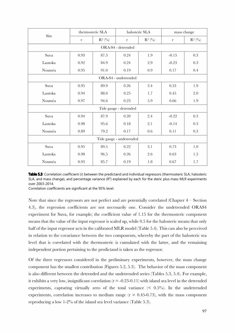
97

Site thermosteric SLA halosteric SLA mass change

r R2 (%) r R2 (%) r R2 (%)

ORA-S4 - detrended

Suva 0.93 87.3 0.24 1.9 -0.15 0.3

Lautoka 0.92 84.9 0.24 2.9 -0.23 0.3

Nouméa 0.95 91.0 0.19 0.9 0.17 0.4


Suva 0.95 89.9 0.26 3.4 0.53 1.9

Lautoka 0.94 88.0 0.25 1.7 0.45 2.0

Nouméa 0.97 94.6 0.23 5.9 0.66 1.9


Suva 0.94 87.9 0.20 2.4 -0.22 0.3

Lautoka 0.98 95.6 0.18 2.1 -0.14 0.3

Nouméa 0.89 79.2 0.17 0.6 0.11 0.3


Suva 0.95 89.5 0.22 3.1 0.73 1.0

Lautoka 0.98 96.5 0.26 2.6 0.63 1.5

Nouméa 0.93 85.7 0.19 1.8 0.67 1.7

Table 5.3: Correlation coefficient (r) between the predictand and individual regressors (thermosteric SLA, halosteric SLA, and mass change), and percentage variance (R2) explained by each for the steric plus mass MLR experiments over 2003-2014. Correlation coefficients are significant at the 95% level. Note that since the regressors are not perfect and are potentially correlated (Chapter 4 – Section 4.3), the regression coefficients are not necessarily one. Consider the undetrended ORAS4 experiment for Suva, for example; the coefficient value of 1.15 for the thermosteric component means that the value of the input regressor is scaled up, while 0.5 for the halosteric means that only half of the input regressor acts in the calibrated MLR model (Table 5.4). This can also be perceived in relation to the covariance between the two components, whereby the part of the halosteric sea level that is correlated with the thermosteric is cumulated with the latter, and the remaining independent portion pertaining to the predictand is taken as the regressor.

Of the three regressors considered in the preliminary experiments, however, the mass change component has the smallest contribution (Figures 5.2, 5.3). The behavior of the mass component is also different between the detrended and the undetrended series (Tables 5.3, 5.4). For example, it exhibits a very low, insignificant correlation (r = -0.23-0.11) with island sea level in the detrended experiments, capturing virtually zero of the total variance (< 0.5%). In the undetrended experiments, correlation increases to medium range (r = 0.45-0.73), with the mass component reproducing a low 1-2% of the island sea level variance (Table 5.3).

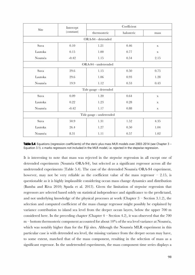
98

Site Intercept (constant)

Coefficient

thermosteric halosteric mass

ORA-S4 - detrended

Suva 0.10 1.21 0.46 x

Lautoka 0.15 1.00 0.77 x

Nouméa -0.42 1.15 0.54 2.15


Suva 29.6 1.15 0.50 0.75

Lautoka 29.6 1.06 0.93 1.28

Nouméa 19.9 1.12 0.53 0.43


Suva 0.09 1.20 0.64 x

Lautoka 0.22 1.23 0.28 x

Nouméa -0.42 1.17 0.88 x


Suva 50.9 1.31 1.52 4.35

Lautoka 26.4 1.27 0.50 1.04

Nouméa 8.31 1.11 0.57 1.02

Table 5.4: Equations (regression coefficients) of the steric plus mass MLR models over 2003-2014 (see Chapter 3 – Equation 3.1). x marks regressors not included in the MLR model, i.e. rejected in the stepwise regression. It is interesting to note that mass was rejected in the stepwise regression in all except one of detrended experiments (Nouméa ORA-S4), but selected as a significant regressor across all the undetrended experiments (Table 5.4). The case of the detrended Nouméa ORA-S4 experiment, however, may not be very reliable as the coefficient value of the mass regressor – 2.15, is questionable as it is highly implausible considering ocean mass change dynamics and distribution (Bamba and Riva 2010; Spada et al. 2013). Given the limitation of stepwise regression that regressors are selected based solely on statistical independence and significance to the predictand, and not underlying knowledge of the physical processes at work (Chapter 3 – Section 3.1.2), the selection and computed coefficient of the mass change regressor might possibly be explained by variance contribution to island sea level from the deeper ocean layers, below the upper 700 m considered here. In the preceding chapter (Chapter 4 – Section 4.2), it was observed that the 700 m – bottom thermosteric component accounted for about 10% of the sea level variance at Nouméa, which was notably higher than for the Fiji sites. Although the Nouméa MLR experiment in this particular case is with detrended sea level, the missing variance from the deeper ocean may have, to some extent, matched that of the mass component, resulting in the selection of mass as a significant regressor. In the undetrended experiments, the mass component time series displays a

99

positive trend, concurrent with a higher correlation and percentage variance than in the detrended case (Figure 5.3). The trend is 1.7 mm/yr, which is 55% of the GMSL trend over the 2003-2014 period (note that the mass change component here has been taken as the globally averaged time series; Chapter 3 – Section 3.6.1). This is also very close to the estimated 1.4-1.6 mm/yr of sea level rise in the western tropical Pacific from ice mass contribution over the last decade (Bamber and Riva 2010). The selection of the mass change component as a significant regressor in all of the undetrended experiments (Table 5.4) indicates that while contribution from mass is still relatively small, it becomes increasingly important when sea level trends are considered.

5.2.1.2 Steric plus mass MLR models

The predictand and modeled sea level time series for the preliminary steric plus mass MLR experiments are shown in Figures 5.4 (detrended) and 5.5 (undetrended). Correlation coefficients between the predictand and the MLR modeled sea levels, and the percentage variance reproduced by the model are shown in Table 5.5. Table 5.6 shows the trends of the predictand and modeled time series for the undetrended experiments.

The MLR modeled sea level time series display high agreement with the predictand (Figures 5.4, 5.5). Correlation coefficients between the two are very high (r ≥ 0.93), with the model explaining a very high 89-98% of the variance (Table 5.5). In addition, the models exhibit good skill in reproducing the predictand sea level trends (0.3-0.4 mm/yr difference) (Table 5.6). These results not only show the efficiency of the MLR approach, but also corroborate thermosteric dominance in island sea level from existing knowledge.

Inter comparison of the model equations (Table 5.4) provides useful insight into the calibration and related skills/limitations of the approach. Since the regressor time series are anomalies relative to the analysis period, 2003-2014, the intercept essentially denotes the difference between the temporal mean over the two periods. So, for example, the intercept value of 29.6 for the Fiji sites in the undetrended ORA-S4 experiments means that the modeled sea level over 2003-2014 was about 29.6 mm higher than that for 1993-2012 on average (Table 5.4).

Throughout the undetrended MLR experiments, unanimously positive intercept values indicate rise in the mean island sea level relative to the 1993-2012 baseline, which is coherent with increasing sea levels in the western Pacific over the recent decades. Notable differences exist between the undetrended ORA-S4 and tide gauge intercepts in the MLR model equations calibrated for the sites Suva and Nouméa (Suva: ORA-S4 = 29.6, tide gauge = 50.9; Nouméa: ORA-S4 = 19.9, tide gauge = 8.31) (Table 5.4), which are most likely due to the aforementioned subsidence and uplift effects in the tide gauge records (Section 5.1). In the undetrended Lautoka ORA-S4 experiment, the halosteric and mass regressor coefficients are relatively high, and might be related to the MLR function calibrating a best fit of the data rather than accounting for a physical mechanism.

100

Figure 5.4: MLR modeled and predictand sea level time series at interannual-to-decadal timescales for the steric plus mass MLR experiments (detrended) over 2003-2014. The modeled time series are shown as red line and the predictand time series as blue lines. A more comprehensive view of the MLR model can thus be obtained by not only evaluating its ability to replicate the predictand, but investigating the calibration specifics (i.e. the regression coefficients). In this way, contribution of individual regressors to the model can be analyzed and compared to existing knowledge as further verification of the MLR model.

These preliminary set of experiments have shown good overall performance of the MLR models and have pinned down some inconsistencies related to biases in the predictand time series that need to be taken into account when interpreting results.

101

Figure 5.5: MLR modeled and predictand sea level time series at interannual-to-decadal timescales for the steric plus mass MLR experiments (undetrended) over 2003-2014. The modeled time series are shown as red line and the predictand time series as blue lines.

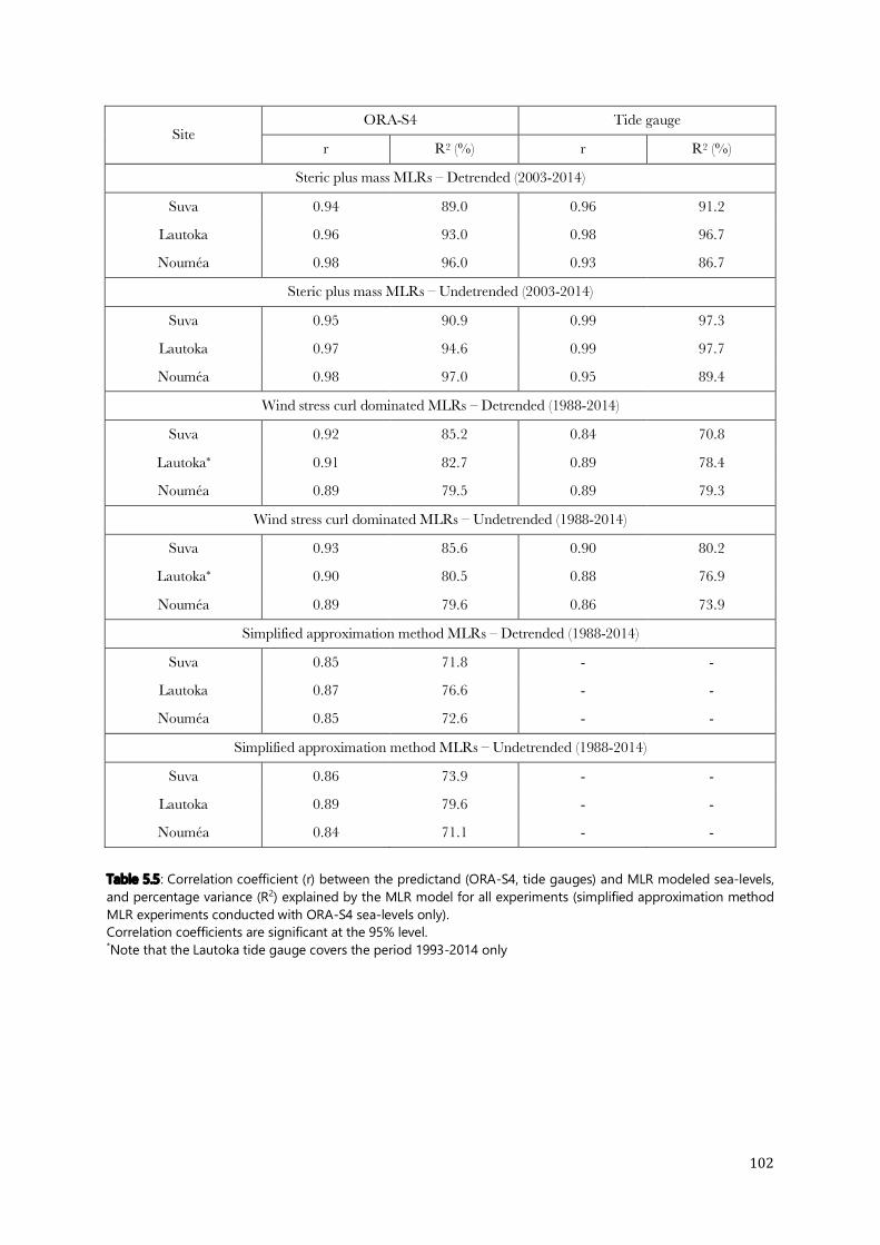
102

Site ORA-S4 Tide gauge

r R2 (%) r R2 (%)

Steric plus mass MLRs – Detrended (2003-2014)

Suva 0.94 89.0 0.96 91.2

Lautoka 0.96 93.0 0.98 96.7

Nouméa 0.98 96.0 0.93 86.7

Steric plus mass MLRs – Undetrended (2003-2014)

Suva 0.95 90.9 0.99 97.3

Lautoka 0.97 94.6 0.99 97.7

Nouméa 0.98 97.0 0.95 89.4

Wind stress curl dominated MLRs – Detrended (1988-2014)

Suva 0.92 85.2 0.84 70.8

Lautoka* 0.91 82.7 0.89 78.4

Nouméa 0.89 79.5 0.89 79.3

Wind stress curl dominated MLRs – Undetrended (1988-2014)

Suva 0.93 85.6 0.90 80.2

Lautoka* 0.90 80.5 0.88 76.9

Nouméa 0.89 79.6 0.86 73.9

Simplified approximation method MLRs – Detrended (1988-2014)

Suva 0.85 71.8 - -

Lautoka 0.87 76.6 - -

Nouméa 0.85 72.6 - -

Simplified approximation method MLRs – Undetrended (1988-2014)

Suva 0.86 73.9 - -

Lautoka 0.89 79.6 - -

Nouméa 0.84 71.1 - -

Table 5.5: Correlation coefficient (r) between the predictand (ORA-S4, tide gauges) and MLR modeled sea-levels, and percentage variance (R2) explained by the MLR model for all experiments (simplified approximation method MLR experiments conducted with ORA-S4 sea-levels only). Correlation coefficients are significant at the 95% level. *Note that the Lautoka tide gauge covers the period 1993-2014 only

103

5.2.2 Wind stress curl (Rossby wave model) dominated MLR models (1988-2014)

In the previous section, it was seen that ocean mass change has a significant contribution to long-term trends in island sea level but has a small contribution to the variability (compare results of the detrended and undetrended series – Section 5.2.1). Thus, the main MLR experiments were extended into the past, the 1988-2014 study period, without a mass regressor. Regarding future scenarios, however, note that the mass contribution will be much higher as warming continues.

The main wind stress curl dominated MLR models take on a process and dynamics based approach, combining wind stress curl as the prevailing regional driver of thermosteric sea level, with the halosteric component, τx, τy, and SST as local modulators.

The predictand and modeled island sea level time series are shown in Figures 5.6 (detrended) and 5.7 (undetrended). The model vs. predictand correlation coefficients and percentage variances explained are included in Table 5.5, and trends of the respective time series in Table 5.6. The calibrated MLR equations are shown in Table 5.7. A supplementary table on correlation between the predictand and individual potential regressors, together with the percentage variance represented by each, corresponding to Table 5.3 (Section 5.2.1.1) for the preliminary experiments is provided in Appendix A.2.

The modeled sea levels exhibit high similarity with the predictands, with comparable results between the detrended and undetrended experiments (Figures 5.6, 5.7, Table 5.5). The MLR modeled time series display slightly better skill when using ORA-S4 sea levels as predictands compared to when tide gauge records are used (Table 5.5). This likely arises from consistency between the predictand and regressor datasets; ERA-Interim fields are used to force ORA-S4 over most of the study period (Chapter 3 – Section 3.4.2.3). For the ORA-S4 experiments, correlation coefficients between the predictand and the modeled sea levels range between 0.89-0.93, and the model is able to explain approximately 82% of the variance on average. For the tide gauge based MLR models, the correlation coefficients range between 0.84-0.90, with an averaged variance of approximately 77% explained by the model (Table 5.5).

In terms of trends (GMSL trend removed), the ORA-S4 Suva and Lautoka MLR modeled sea levels are very close to the predictands (0.2 mm/yr difference) (Table 5.6). For Nouméa ORA-S4, however, the difference is more pronounced (0.4 mm/yr difference). The Nouméa ORA-S4 correlation coefficient and percentage variance explained are also slightly lower compared to the Fiji sites (Table 5.5). This is most likely related to the location of the Nouméa site (22 °S) at a lower latitude than Fiji (17- 18 °S), where the Rossby wave energy would be slightly lower, corresponding to a lowered approximation of thermocline movement induced thermosteric sea level change (e.g. White at al. 1985; Rebert et al. 1985; Palanisamy et al. 2015a).

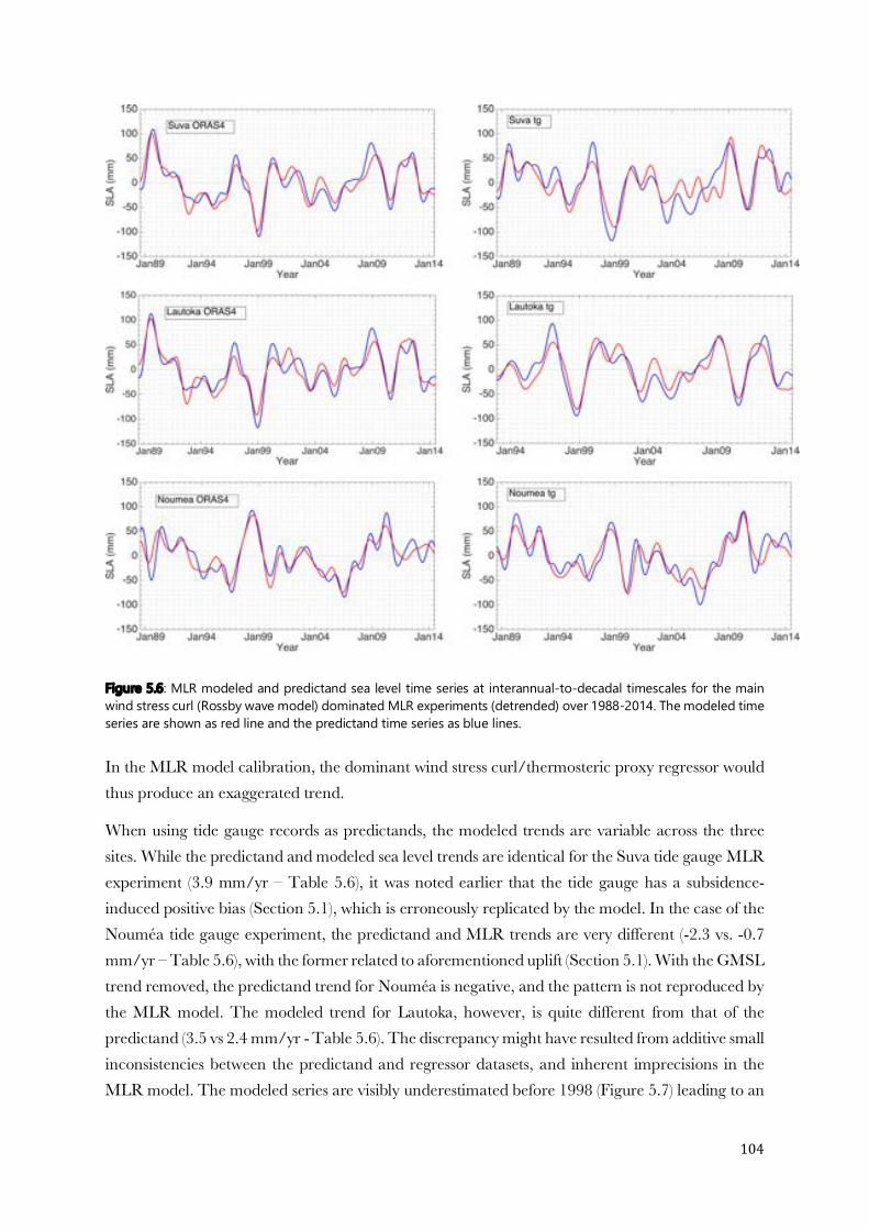
104

Figure 5.6: MLR modeled and predictand sea level time series at interannual-to-decadal timescales for the main wind stress curl (Rossby wave model) dominated MLR experiments (detrended) over 1988-2014. The modeled time series are shown as red line and the predictand time series as blue lines. In the MLR model calibration, the dominant wind stress curl/thermosteric proxy regressor would thus produce an exaggerated trend.

When using tide gauge records as predictands, the modeled trends are variable across the three sites. While the predictand and modeled sea level trends are identical for the Suva tide gauge MLR experiment (3.9 mm/yr – Table 5.6), it was noted earlier that the tide gauge has a subsidence-induced positive bias (Section 5.1), which is erroneously replicated by the model. In the case of the Nouméa tide gauge experiment, the predictand and MLR trends are very different (-2.3 vs. -0.7 mm/yr – Table 5.6), with the former related to aforementioned uplift (Section 5.1). With the GMSL trend removed, the predictand trend for Nouméa is negative, and the pattern is not reproduced by the MLR model. The modeled trend for Lautoka, however, is quite different from that of the predictand (3.5 vs 2.4 mm/yr - Table 5.6). The discrepancy might have resulted from additive small inconsistencies between the predictand and regressor datasets, and inherent imprecisions in the MLR model. The modeled series are visibly underestimated before 1998 (Figure 5.7) leading to an

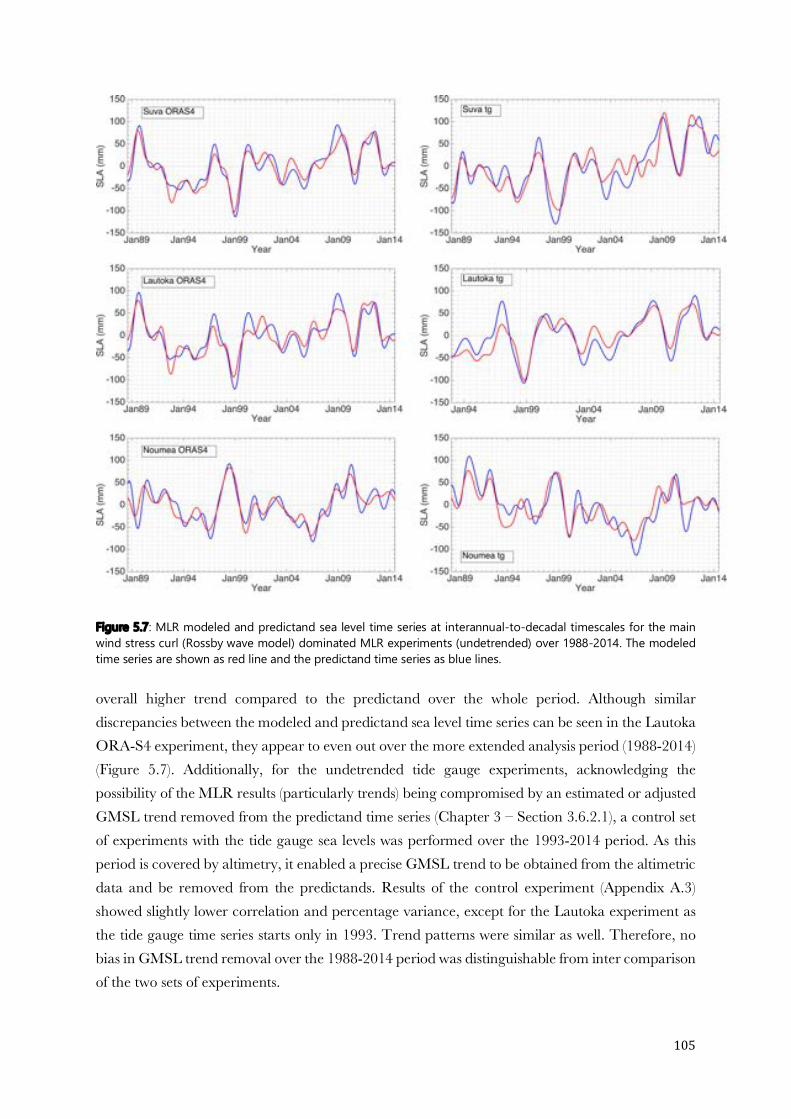
105

Figure 5.7: MLR modeled and predictand sea level time series at interannual-to-decadal timescales for the main wind stress curl (Rossby wave model) dominated MLR experiments (undetrended) over 1988-2014. The modeled time series are shown as red line and the predictand time series as blue lines. overall higher trend compared to the predictand over the whole period. Although similar discrepancies between the modeled and predictand sea level time series can be seen in the Lautoka ORA-S4 experiment, they appear to even out over the more extended analysis period (1988-2014) (Figure 5.7). Additionally, for the undetrended tide gauge experiments, acknowledging the possibility of the MLR results (particularly trends) being compromised by an estimated or adjusted GMSL trend removed from the predictand time series (Chapter 3 – Section 3.6.2.1), a control set of experiments with the tide gauge sea levels was performed over the 1993-2014 period. As this period is covered by altimetry, it enabled a precise GMSL trend to be obtained from the altimetric data and be removed from the predictands. Results of the control experiment (Appendix A.3) showed slightly lower correlation and percentage variance, except for the Lautoka experiment as the tide gauge time series starts only in 1993. Trend patterns were similar as well. Therefore, no bias in GMSL trend removal over the 1988-2014 period was distinguishable from inter comparison of the two sets of experiments.

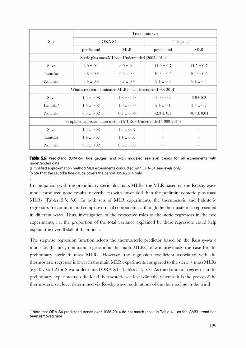
106

Site

Trend (mm/yr)

ORA-S4 Tide gauge

predictand MLR predictand MLR

Steric plus mass MLRs – Undetrended (2003-2014)

Suva 8.0 ± 0.4 8.0 ± 0.4 14.9 ± 0.7 14.5 ± 0.7

Lautoka 6.8 ± 0.3 6.6 ± 0.3 10.3 ± 0.5 10.0 ± 0.5

Nouméa 8.4 ± 0.4 8.7 ± 0.4 9.4 ± 0.5 9.4 ± 0.5


Suva 1.6 ± 0.08 1.8 ± 0.09 3.9 ± 0.2 3.9± 0.2

Lautoka* 1.4 ± 0.07 1.6 ± 0.08 2.4 ± 0.1 3.5 ± 0.2

Nouméa 0.3 ± 0.02 0.7 ± 0.04 -2.3 ± 0.1 -0.7 ± 0.04


Suva 1.6 ± 0.08 1.3 ± 0.07 - -

Lautoka 1.4 ± 0.07 1.4 ± 0.07 - -

Nouméa 0.3 ± 0.02 0.6 ± 0.03 - -

Table 5.6: Predictand (ORA-S4, tide gauges) and MLR modeled sea-level trends for all experiments with undetrended data*. (simplified approximation method MLR experiments conducted with ORA-S4 sea-levels only). *Note that the Lautoka tide gauge covers the period 1993-2014 only. . In comparison with the preliminary steric plus mass MLRs, the MLR based on the Rossby wave model produced good results, nevertheless with lower skill than the preliminary steric plus mass MLRs (Tables 5.5, 5.6). In both sets of MLR experiments, the thermosteric and halosteric regressors are common and comprise crucial components, although the thermosteric is represented in different ways. Thus, investigation of the respective roles of the steric regressors in the two experiments, i.e. the proportion of the total variance explained by these regressors could help explain the overall skill of the models.

The stepwise regression function selects the thermosteric predictor based on the Rossby-wave model as the first, dominant regressor in the main MLRs, as was previously the case for the preliminary steric + mass MLRs. However, the regression coefficient associated with the thermosteric regressor is lower in the main MLR experiments compared to the steric + mass MLRs (e.g. 0.7 vs 1.2 for Suva undetrended ORA-S4 - Tables 5.4, 5.7). As the dominant regressor in the preliminary experiments is the local thermosteric sea level directly, whereas it is the proxy of the thermosteric sea level determined via Rossby wave modulations of the thermocline in the wind

* Note that ORA-S4 predictand trends over 1988-2014 do not match those in Table 4.1 as the GMSL trend has been removed here

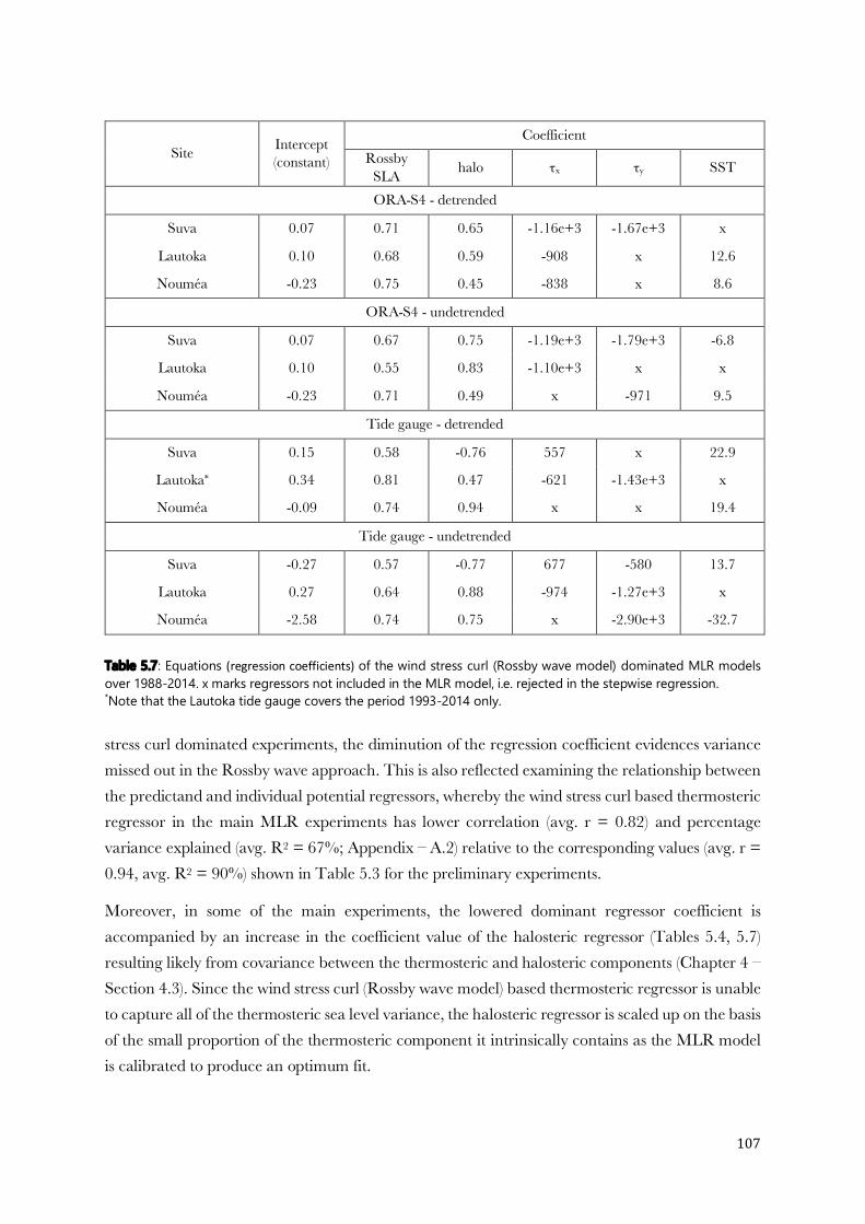
107

Table 5.7: Equations (regression coefficients) of the wind stress curl (Rossby wave model) dominated MLR models over 1988-2014. x marks regressors not included in the MLR model, i.e. rejected in the stepwise regression. *Note that the Lautoka tide gauge covers the period 1993-2014 only. stress curl dominated experiments, the diminution of the regression coefficient evidences variance missed out in the Rossby wave approach. This is also reflected examining the relationship between the predictand and individual potential regressors, whereby the wind stress curl based thermosteric regressor in the main MLR experiments has lower correlation (avg. r = 0.82) and percentage variance explained (avg. R2 = 67%; Appendix – A.2) relative to the corresponding values (avg. r = 0.94, avg. R2 = 90%) shown in Table 5.3 for the preliminary experiments.

Moreover, in some of the main experiments, the lowered dominant regressor coefficient is accompanied by an increase in the coefficient value of the halosteric regressor (Tables 5.4, 5.7) resulting likely from covariance between the thermosteric and halosteric components (Chapter 4 – Section 4.3). Since the wind stress curl (Rossby wave model) based thermosteric regressor is unable to capture all of the thermosteric sea level variance, the halosteric regressor is scaled up on the basis of the small proportion of the thermosteric component it intrinsically contains as the MLR model is calibrated to produce an optimum fit.


Coefficient Rossby

SLA halo τx τy SST

ORA-S4 - detrended

Suva 0.07 0.71 0.65 -1.16e+3 -1.67e+3 x

Lautoka 0.10 0.68 0.59 -908 x 12.6

Nouméa -0.23 0.75 0.45 -838 x 8.6


Suva 0.07 0.67 0.75 -1.19e+3 -1.79e+3 -6.8

Lautoka 0.10 0.55 0.83 -1.10e+3 x x

Nouméa -0.23 0.71 0.49 x -971 9.5


Suva 0.15 0.58 -0.76 557 x 22.9

Lautoka* 0.34 0.81 0.47 -621 -1.43e+3 x

Nouméa -0.09 0.74 0.94 x x 19.4


Suva -0.27 0.57 -0.77 677 -580 13.7

Lautoka 0.27 0.64 0.88 -974 -1.27e+3 x

Nouméa -2.58 0.74 0.75 x -2.90e+3 -32.7

108

Figure 5.8: Site-based thermosteric sea level and wind stress curl (Rossby wave model) proxy based thermosteric regressor time series at interannual-to-decadal timescales for the main MLR experiments (detrended) over 1988-2014. The thermosteric time series are shown as red lines and the wind stress curl proxy time series as turquoise lines. The efficiency of the Rossby wave model is further explored by comparing its thermosteric component with that of the preliminary experiment, as illustrated in Figures 5.8 (detrended) and 5.9 (undetrended). Correlation coefficients between the two and the percentage variance represented by the wind stress curl based thermosteric regressor are shown in Table 5.8.

Though the thermosteric sea level and wind stress curl based regressor time series are overall similar and have high correlation with each other (r = 0.86-0.91), there are distinct differences in amplitude and in the phasing of their interannual variability (Figures 5.8, 5.9, Table 5.8). The wind stress curl based regressor captures 75-83% of the thermosteric variance. A certain degree of discrepancy is expected between the actual and the wind stress curl induced thermosteric change, notably due to the thickening of the thermocline and increase in stratification when moving away from the equator, with optimum correlations generally found within the 15° tropical band (White et al. 1985; Rebert et al. 1985; Palanisamy et al. 2015a).

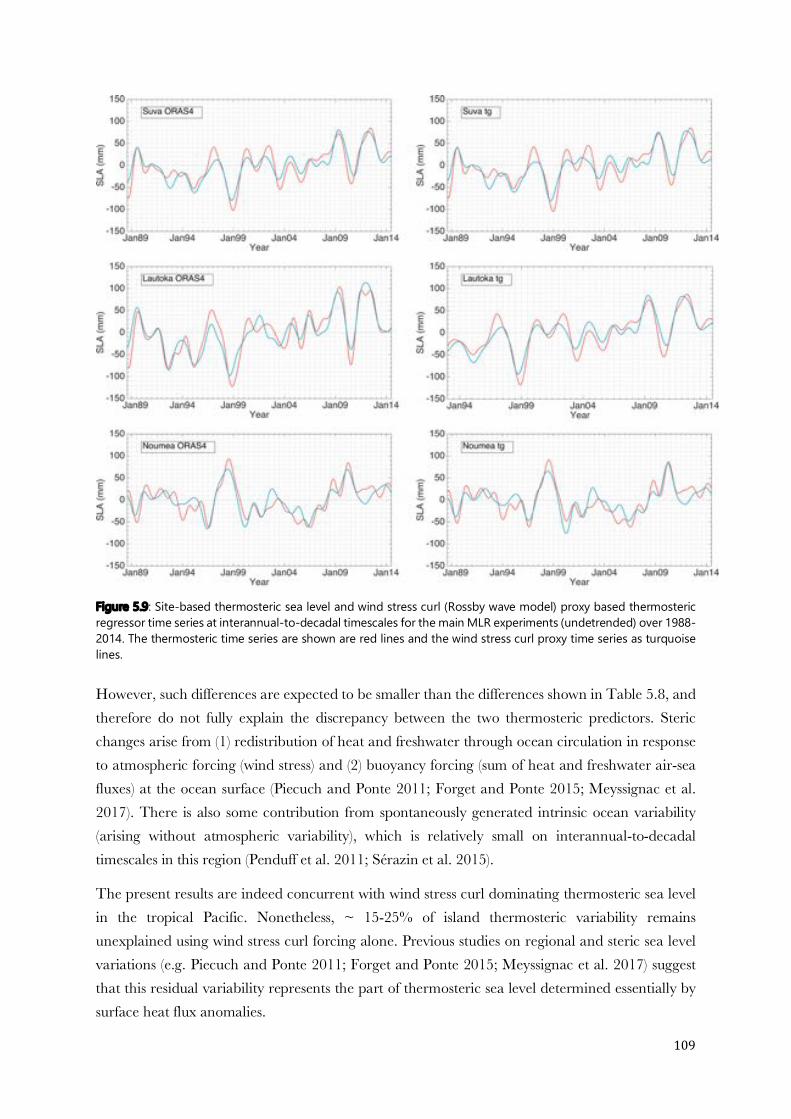
109

Figure 5.9: Site-based thermosteric sea level and wind stress curl (Rossby wave model) proxy based thermosteric regressor time series at interannual-to-decadal timescales for the main MLR experiments (undetrended) over 1988-2014. The thermosteric time series are shown are red lines and the wind stress curl proxy time series as turquoise lines. However, such differences are expected to be smaller than the differences shown in Table 5.8, and therefore do not fully explain the discrepancy between the two thermosteric predictors. Steric changes arise from (1) redistribution of heat and freshwater through ocean circulation in response to atmospheric forcing (wind stress) and (2) buoyancy forcing (sum of heat and freshwater air-sea fluxes) at the ocean surface (Piecuch and Ponte 2011; Forget and Ponte 2015; Meyssignac et al. 2017). There is also some contribution from spontaneously generated intrinsic ocean variability (arising without atmospheric variability), which is relatively small on interannual-to-decadal timescales in this region (Penduff et al. 2011; Sérazin et al. 2015).

The present results are indeed concurrent with wind stress curl dominating thermosteric sea level in the tropical Pacific. Nonetheless, ~ 15-25% of island thermosteric variability remains unexplained using wind stress curl forcing alone. Previous studies on regional and steric sea level variations (e.g. Piecuch and Ponte 2011; Forget and Ponte 2015; Meyssignac et al. 2017) suggest that this residual variability represents the part of thermosteric sea level determined essentially by surface heat flux anomalies.

110

Site ORA-S4 Tide gauge

r R2 (%) r R2 (%)

Wind stress curl dominated MLRs – Detrended (1988-2014)

Suva 0.86 74.6 0.86 74.7

Lautoka* 0.89 79.6 0.89 78.8

Nouméa 0.86 74.4 0.87 75.2


Suva 0.90 80.3 0.88 77.6

Lautoka* 0.91 82.5 0.91 83.3

Nouméa 0.87 75.1 0.86 74.5

Simplified approximation method MLRs – Detrended (1988-2014)

Suva 0.59 34.7 - -

Lautoka 0.69 47.6 - -

Nouméa 0.66 43.0 - -


Suva 0.55 30.6 - -

Lautoka 0.64 40.4 - -

Nouméa 0.59 35.0 - -

Table 5.8: Correlation coefficient (r) between the thermosteric sea-level and wind stress curl regressor (Rossby wave model derived thermosteric approximated proxy), and percentage variance (R2) explained by the thermosteric proxy for the wind stress curl dominated and the simplified approximation method MLR experiments (conducted with ORA-S4 sea-levels only). Correlation coefficients are significant at the 95% level. *Note that the Lautoka tide gauge covers the period 1993-2014 only. Following the dominant Rossby wave model based thermosteric regressor, the halosteric sea level is selected as a significant regressor throughout all the experiments (Table 5.7). This is consistent with the deterministic role of the total steric component in sea level variations. Regressed onto the island sea levels, the strength of the individual halosteric predictor varies across the Fiji sites and Nouméa, with relatively larger influence at the former. (Appendix – A.2). The halosteric regressor coefficients vary across the different experiments and sites (0.45-0.94 range), however, anomalously negative values are seen in both the Suva tide gauge experiments (detrended: -0.76, undetrended: -0.77 – Table 5.7). The Suva halosteric coefficients bear great contrast to other sites and corresponding preliminary experiments, all of which display positive values (Tables 5.4, 5.7). The negative coefficients in this case are believed to have culminated from the combined effects of the positive biases in the Suva tide gauge record, (Section 5.1) and the absence of in-built knowledge of underlying physical mechanisms at work in the regression model as it calibrates a best fit of the input data (Chapter 3 – Section 3.1.2).

111

Unlike the proxy thermosteric and halosteric regressors, selection of the rest of the regressors (τx, τy, SST) is mostly inconsistent across the different experiments, even for the same sites (Table 5.7). Different combinations of these regressors for the same sites moving from the detrended to the undetrended experiments could be interpreted as inclusion of additional variables contributing to the rising trend in the latter, and subsequent rejection of initially selected regressors in the detrended experiments in cases of multi-collinearity. However, selected regressor combinations are different in the ORA-S4 and the tide gauge based detrended experiments for the same sites (Table 5.7). The selected regressors are also different for the Suva and Lautoka sites, which are located very close to each other and display very similar sea level variations. Experiments conducted with the Suva tide gauge predictands in particular, in addition to the aforementioned negative coefficients for the halosteric regressor, display positive values for the zonal wind stress regressor in contrast to the rest of the experiments (zonal wind stress positive towards the east in the dataset). This incorrectly implies that strengthening of the easterlies leads to shoaling of the western basin thermocline thus lowering of sea levels, and vice-versa. For the local scale zonal wind stress effects considered here, a negative correlation with island sea level represents part of the wind set-up, whereby waters pile up around the study sites at the western end with an easterly wind flow. For Nouméa, while wind stress forcing dominates sea level variations, contribution from buoyancy forcing (surface heat flux anomalies in particular) to steric variability is higher relative to Fiji (Piecuch and Ponte 2011; Meyssignac et al. 2017). The continual selection of SST in all of the MLR experiments for Nouméa reflects this (Table 5.7); reversal of the SST coefficient sign in the undetrended tide gauge experiment, however, is abnormal and is most likely due to the aforementioned uplift (Section 5.1). The relationship between island sea levels and locally acting wind stress or SST is difficult to robustly identify from the current results.

Overall, the Rossby wave model based MLRs are able to skillfully estimate the island sea level interannual-to-decadal variations, capturing about 78% of the variance on average. While the performance of the wind stress curl dominated MLR models is notably lower than the preliminary MLR models based on steric and mass regressors only, a lowering of model skill to some extent is indeed expected when employing a proxy for the dominant thermosteric component. Examination of the models’ calibration specifics reflects the findings of existing literature that the island sea level variations are essentially steric in nature, however, the precise role of non-dominant, locally acting wind stress and SST in modulating island sea levels remains ambiguous.

5.2.3 Simplified approximation method MLRs (1988-2014)

The MLR models presented in this section have wind stress curl as the dominant regressor, however, unlike in the previous section (main MLR experiments) the wind stress curl is used directly, without incorporation of the Rossby wave model. The aim is to test the skill of a simpler model.

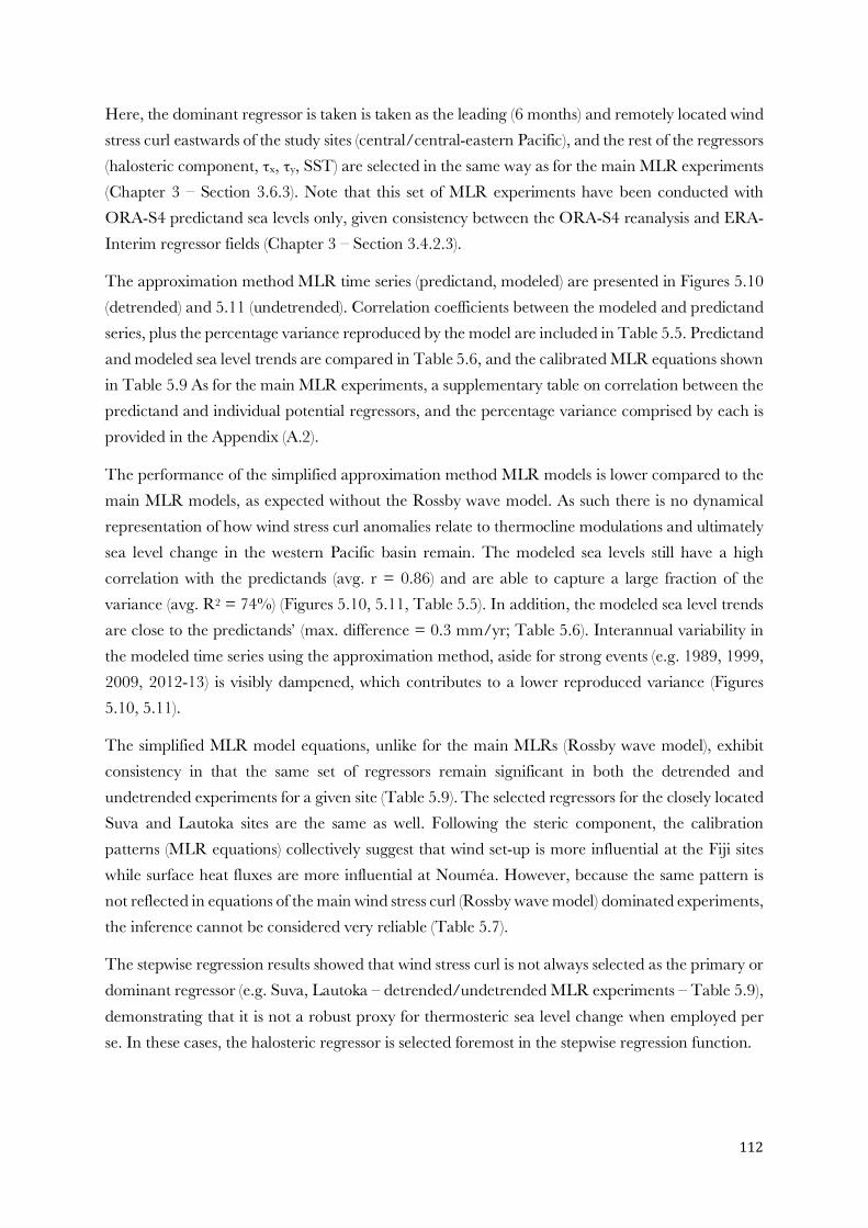
112

Here, the dominant regressor is taken is taken as the leading (6 months) and remotely located wind stress curl eastwards of the study sites (central/central-eastern Pacific), and the rest of the regressors (halosteric component, τx, τy, SST) are selected in the same way as for the main MLR experiments (Chapter 3 – Section 3.6.3). Note that this set of MLR experiments have been conducted with ORA-S4 predictand sea levels only, given consistency between the ORA-S4 reanalysis and ERA-Interim regressor fields (Chapter 3 – Section 3.4.2.3).

The approximation method MLR time series (predictand, modeled) are presented in Figures 5.10 (detrended) and 5.11 (undetrended). Correlation coefficients between the modeled and predictand series, plus the percentage variance reproduced by the model are included in Table 5.5. Predictand and modeled sea level trends are compared in Table 5.6, and the calibrated MLR equations shown in Table 5.9 As for the main MLR experiments, a supplementary table on correlation between the predictand and individual potential regressors, and the percentage variance comprised by each is provided in the Appendix (A.2).

The performance of the simplified approximation method MLR models is lower compared to the main MLR models, as expected without the Rossby wave model. As such there is no dynamical representation of how wind stress curl anomalies relate to thermocline modulations and ultimately sea level change in the western Pacific basin remain. The modeled sea levels still have a high correlation with the predictands (avg. r = 0.86) and are able to capture a large fraction of the variance (avg. R2 = 74%) (Figures 5.10, 5.11, Table 5.5). In addition, the modeled sea level trends are close to the predictands’ (max. difference = 0.3 mm/yr; Table 5.6). Interannual variability in the modeled time series using the approximation method, aside for strong events (e.g. 1989, 1999, 2009, 2012-13) is visibly dampened, which contributes to a lower reproduced variance (Figures 5.10, 5.11).

The simplified MLR model equations, unlike for the main MLRs (Rossby wave model), exhibit consistency in that the same set of regressors remain significant in both the detrended and undetrended experiments for a given site (Table 5.9). The selected regressors for the closely located Suva and Lautoka sites are the same as well. Following the steric component, the calibration patterns (MLR equations) collectively suggest that wind set-up is more influential at the Fiji sites while surface heat fluxes are more influential at Nouméa. However, because the same pattern is not reflected in equations of the main wind stress curl (Rossby wave model) dominated experiments, the inference cannot be considered very reliable (Table 5.7).

The stepwise regression results showed that wind stress curl is not always selected as the primary or dominant regressor (e.g. Suva, Lautoka – detrended/undetrended MLR experiments – Table 5.9), demonstrating that it is not a robust proxy for thermosteric sea level change when employed per se. In these cases, the halosteric regressor is selected foremost in the stepwise regression function.

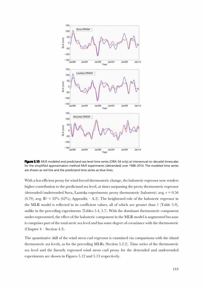
113

Figure 5.10: MLR modeled and predictand sea level time series (ORA-S4 only) at interannual-to-decadal timescales for the simplified approximation method MLR experiments (detrended) over 1988-2014. The modeled time series are shown as red line and the predictand time series as blue lines. With a less efficient proxy for wind forced thermosteric change, the halosteric regressor now renders higher contribution to the predictand sea level, at times surpassing the proxy thermosteric regressor (detrended/undetrended Suva, Lautoka experiments: proxy thermosteric (halosteric) avg. r = 0.56 (0.79), avg. R2 = 32% (62%); Appendix – A.2). The heightened role of the halosteric regressor in the MLR model is reflected in its coefficient values, all of which are greater than 1 (Table 5.9), unlike in the preceding experiments (Tables 5.4, 5.7). With the dominant thermosteric component under-represented, the effect of the halosteric component in the MLR model is augmented because it comprises part of the total steric sea level and has some degree of covariance with the thermosteric (Chapter 4 – Section 4.3).

The quantitative skill of the wind stress curl regressor is examined via comparisons with the island thermosteric sea levels, as for the preceding MLRs (Section 5.2.2). Time series of the thermosteric sea level and the linearly regressed wind stress curl proxy for the detrended and undetrended experiments are shown in Figures 5.12 and 5.13 respectively.

114

Figure 5.11: MLR modeled and predictand sea level time series (ORA-S4 only) at interannual-to-decadal timescales for the simplified approximation method MLR experiments (undetrended) over 1988-2014. The modeled time series are shown as red line and the predictand time series as blue lines


Coefficient

curlz τ halo τx τy SST

ORA-S4 - detrended

Suva 0.07 4.71e+8 1.45 -2.43e+3 -2.80e+3 x

Lautoka 0.10 6.40e+8 1.48 -1.91e+3 -2.44e+3 x

Nouméa -0.23 1.06e+9 1.20 -442.74 x 45.82


Suva 0.07 5.47e+8 1.30 -2.37e+3 -3.10e+3 x

Lautoka 0.10 7.95e+8 1.29 -1.85e+3 -2.72e+3 x

Nouméa -0.23 1.15e+9 1.10 -298.52 x 40.35

Table 5.9: Equations (regression coefficients) of the simplified approximation method MLR models over 1988-2014. x marks regressors not included in the MLR model.

115

Figure 5.12: Site-based thermosteric sea level and wind stress curl proxy based thermosteric regressor time series at interannual-to-decadal timescales for the simplified approximation method MLR experiments (detrended) over 1988-2014. The thermosteric time series are shown are red lines and the wind stress curl proxy time series as turquoise lines. Correlation coefficients between the two and the percentage variance constituted by the wind stress curl proxy are included in Table 5.8.

While similarity does exist between the linearly regressed wind stress curl proxy time series and the island thermosteric sea levels (Figures 5.12, 5.13), discrepancies between the two are notably higher compared to the corresponding plots for the main MLR experiments (Rossby wave model) (Figures 5.8, 5.9). This comparison in particular encapsulates the fundamental difference between the two sets of experiments (main – Section 5.2.2, simplified approximation method – Section 5.2.3), illustrating the respective abilities of the two approaches at replicating thermosteric sea level variations. Correlation between the wind stress curl proxy and the thermosteric sea level is of medium range (avg. r = 0.62), with less than half of the total variance in the latter represented (avg. R2 = 39%) (Table 5.8). Both of the metrics exhibit marked reduction from the corresponding values in the main MLR experiments (Rossby wave model – avg. r = 0.88, avg. R2 = 78%) (Table 5.8).

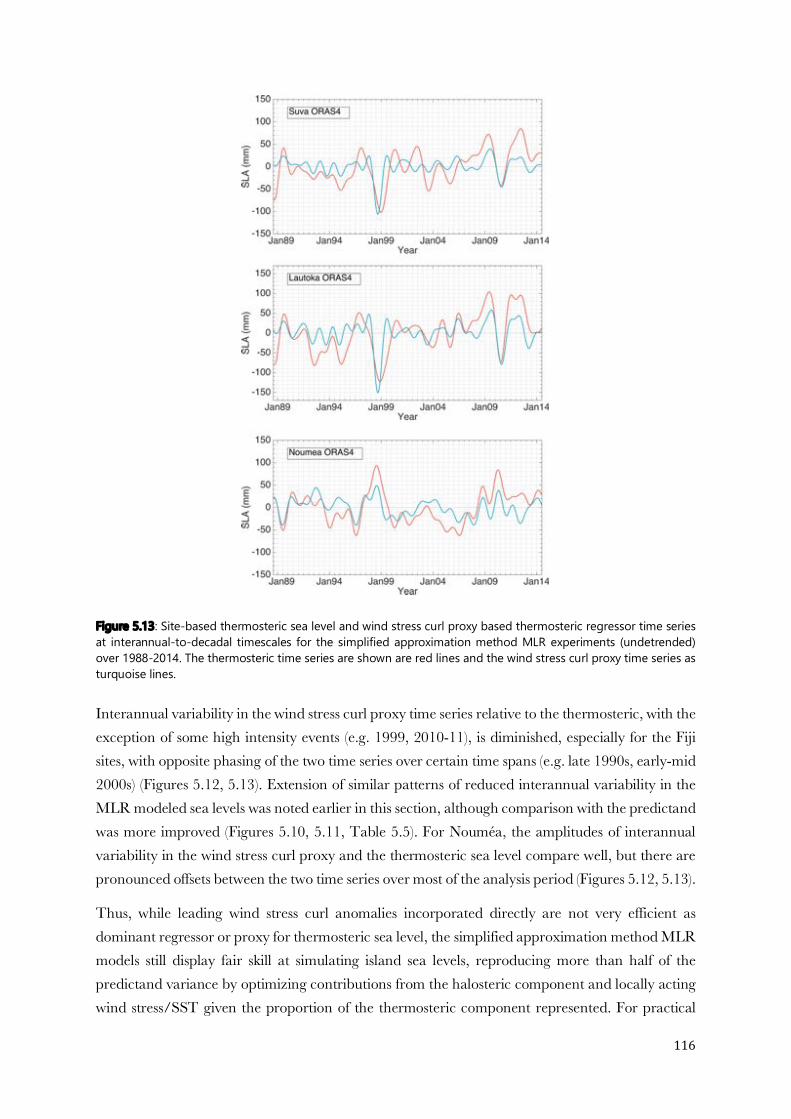
116

Figure 5.13: Site-based thermosteric sea level and wind stress curl proxy based thermosteric regressor time series at interannual-to-decadal timescales for the simplified approximation method MLR experiments (undetrended) over 1988-2014. The thermosteric time series are shown are red lines and the wind stress curl proxy time series as turquoise lines. Interannual variability in the wind stress curl proxy time series relative to the thermosteric, with the exception of some high intensity events (e.g. 1999, 2010-11), is diminished, especially for the Fiji sites, with opposite phasing of the two time series over certain time spans (e.g. late 1990s, early-mid 2000s) (Figures 5.12, 5.13). Extension of similar patterns of reduced interannual variability in the MLR modeled sea levels was noted earlier in this section, although comparison with the predictand was more improved (Figures 5.10, 5.11, Table 5.5). For Nouméa, the amplitudes of interannual variability in the wind stress curl proxy and the thermosteric sea level compare well, but there are pronounced offsets between the two time series over most of the analysis period (Figures 5.12, 5.13).

Thus, while leading wind stress curl anomalies incorporated directly are not very efficient as dominant regressor or proxy for thermosteric sea level, the simplified approximation method MLR models still display fair skill at simulating island sea levels, reproducing more than half of the predictand variance by optimizing contributions from the halosteric component and locally acting wind stress/SST given the proportion of the thermosteric component represented. For practical

117

applications, the main MLR models presented in the preceding section (Section 5.2.2) are undoubtedly better suited of the two as they offer a more robust approach by employing a Rossby wave model and therefore generate more realistic simulations. Nonetheless, the simplified approximation method MLR models have demonstrated that a fair estimate of island sea levels can indeed be obtained using a combination of oceanic/atmospheric variables only.

5.3 Stationarity Test

A stationarity test was incorporated in the analysis to examine the applicability of the MLR models to future projections, i.e. testing the skill of the model over a period other than which it was calibrated over.

Results of the stationarity test are illustrated as MLR modeled time series over each of the two halves of the analysis period, superimposed on the original predictand and modeled sea levels. The stationarity test was conducted on the main wind stress curl (Rossby wave model) dominated experiments and the simplified approximation method experiments, which span over two decades (1988-2014) and thus suffice the minimum duration of data required for a test assessing interannual-to-decadal scale variability. The 1988-2014 analysis period was divided into halves spanning (1) August 1988 – July 2001 and (2) August 2001 – Jul 2014 (note exception for Lautoka tide gauge experiments, 1993-2014 analysis period divided into January 1993 – October 2003 and November 2003 – July 2014). The stationarity test essentially involved calibrating an MLR model using the same set of regressors as the original model over one half of the dataset and applying it to the other, and examining model performance with respect to the predictand and to the original MLR over that period. An MLR model calibrated over a particular half of the dataset is hereafter referred to as the “calibrated” model, and a model calibrated over one half but applied to another is referred to as the “reconstructed” model. The MLR modeled sea levels presented as main results in the previous sections (and calibrated over the entire period) will be referred to as the “original” models where comparisons are drawn with the stationarity test models (calibrated and reconstructed).

The stationarity test time series for the main wind stress curl (Rossby wave model) dominated MLR models are presented in Figures 5.14 (detrended) and 5.15 (undetrended), and for the simplified approximation method MLR models in Figures 5.16 (detrended) and 5.17 (undetrended). With the initially presented predictand and original MLR modeled sea levels aside (blue and red lines), solid lines indicate calibrated models while dashed lines indicate reconstructed models (magenta lines for the models calibrated over the 1st half and applied to the 2nd half of the period, and green lines for the models calibrated over the 2nd half and applied to the 1st half of the period). As for the MLR experiments, evaluation statistics (r, R2, trends) have been drawn for the stationarity test models over each half of the analysis period to allow comparison with the original results.

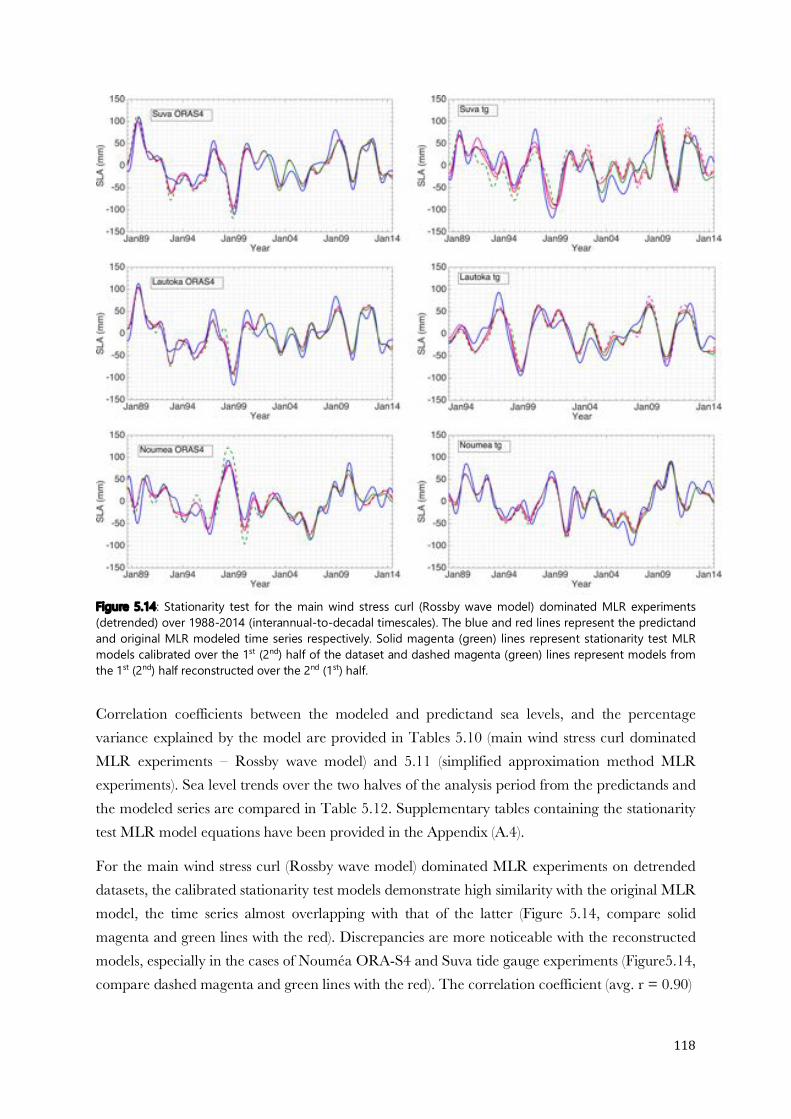
118

Figure 5.14: Stationarity test for the main wind stress curl (Rossby wave model) dominated MLR experiments (detrended) over 1988-2014 (interannual-to-decadal timescales). The blue and red lines represent the predictand and original MLR modeled time series respectively. Solid magenta (green) lines represent stationarity test MLR models calibrated over the 1st (2nd) half of the dataset and dashed magenta (green) lines represent models from the 1st (2nd) half reconstructed over the 2nd (1st) half. Correlation coefficients between the modeled and predictand sea levels, and the percentage variance explained by the model are provided in Tables 5.10 (main wind stress curl dominated MLR experiments – Rossby wave model) and 5.11 (simplified approximation method MLR experiments). Sea level trends over the two halves of the analysis period from the predictands and the modeled series are compared in Table 5.12. Supplementary tables containing the stationarity test MLR model equations have been provided in the Appendix (A.4).

For the main wind stress curl (Rossby wave model) dominated MLR experiments on detrended datasets, the calibrated stationarity test models demonstrate high similarity with the original MLR model, the time series almost overlapping with that of the latter (Figure 5.14, compare solid magenta and green lines with the red). Discrepancies are more noticeable with the reconstructed models, especially in the cases of Nouméa ORA-S4 and Suva tide gauge experiments (Figure5.14, compare dashed magenta and green lines with the red). The correlation coefficient (avg. r = 0.90)

119

Figure 5.15: Stationarity test for the main wind stress curl (Rossby wave model) dominated MLR experiments (undetrended) over 1988-2014 (interannual-to-decadal timescales). The blue and red lines represent the predictand and modeled time series respectively. Solid magenta (green) lines represent stationarity test MLR models calibrated over the 1st (2nd) half of the dataset and dashed magenta (green) lines represent models from the 1st (2nd) half reconstructed over the 2nd (1st) half. and percentage variance (avg. R2 = 81%) reproduced by the stationarity test calibrated models are comparable to the original MLR models (Table 5.10). The corresponding metrics for the reconstructed models are generally lower (avg. r = 0.88, R2 = 64%), as reflected in the time series. Particularly for the reconstructed models on the 1st half of the series, the variance relative to that of the predictand is generally over-estimated.

For the undetrended wind stress curl (Rossby wave model) dominated MLR experiments, the calibrated stationarity test models show little change from the detrended experiments, maintaining high resemblance to the original MLR models (Figure 5.15, compare solid magenta and green lines with the red). Correlation between the calibrated and predictand sea levels remains high (avg. r = 0.91), with the latter successfully reproducing the larger majority of the predictand variance (avg. R2 = 82%) (Table 5.10). On the other hand, differences between the reconstructed and original MLR time series are more distinct, particularly for the tide gauge experiments and Nouméa ORA-S4 (Figure 5.15, compare dashed magenta and green lines with the red).

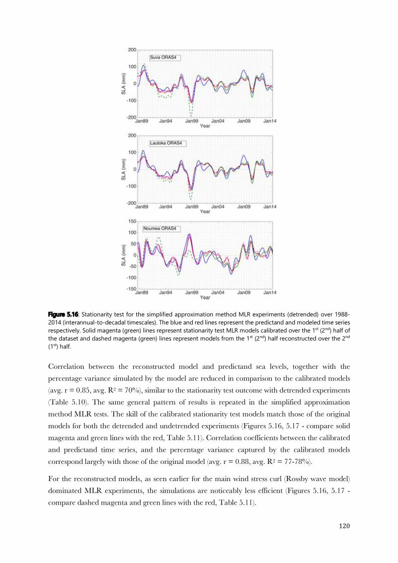
120

Figure 5.16: Stationarity test for the simplified approximation method MLR experiments (detrended) over 1988-2014 (interannual-to-decadal timescales). The blue and red lines represent the predictand and modeled time series respectively. Solid magenta (green) lines represent stationarity test MLR models calibrated over the 1st (2nd) half of the dataset and dashed magenta (green) lines represent models from the 1st (2nd) half reconstructed over the 2nd (1st) half. Correlation between the reconstructed model and predictand sea levels, together with the percentage variance simulated by the model are reduced in comparison to the calibrated models (avg. r = 0.85, avg. R2 = 70%), similar to the stationarity test outcome with detrended experiments (Table 5.10). The same general pattern of results is repeated in the simplified approximation method MLR tests. The skill of the calibrated stationarity test models match those of the original models for both the detrended and undetrended experiments (Figures 5.16, 5.17 - compare solid magenta and green lines with the red, Table 5.11). Correlation coefficients between the calibrated and predictand time series, and the percentage variance captured by the calibrated models correspond largely with those of the original model (avg. r = 0.88, avg. R2 = 77-78%).

For the reconstructed models, as seen earlier for the main wind stress curl (Rossby wave model) dominated MLR experiments, the simulations are noticeably less efficient (Figures 5.16, 5.17 - compare dashed magenta and green lines with the red, Table 5.11).

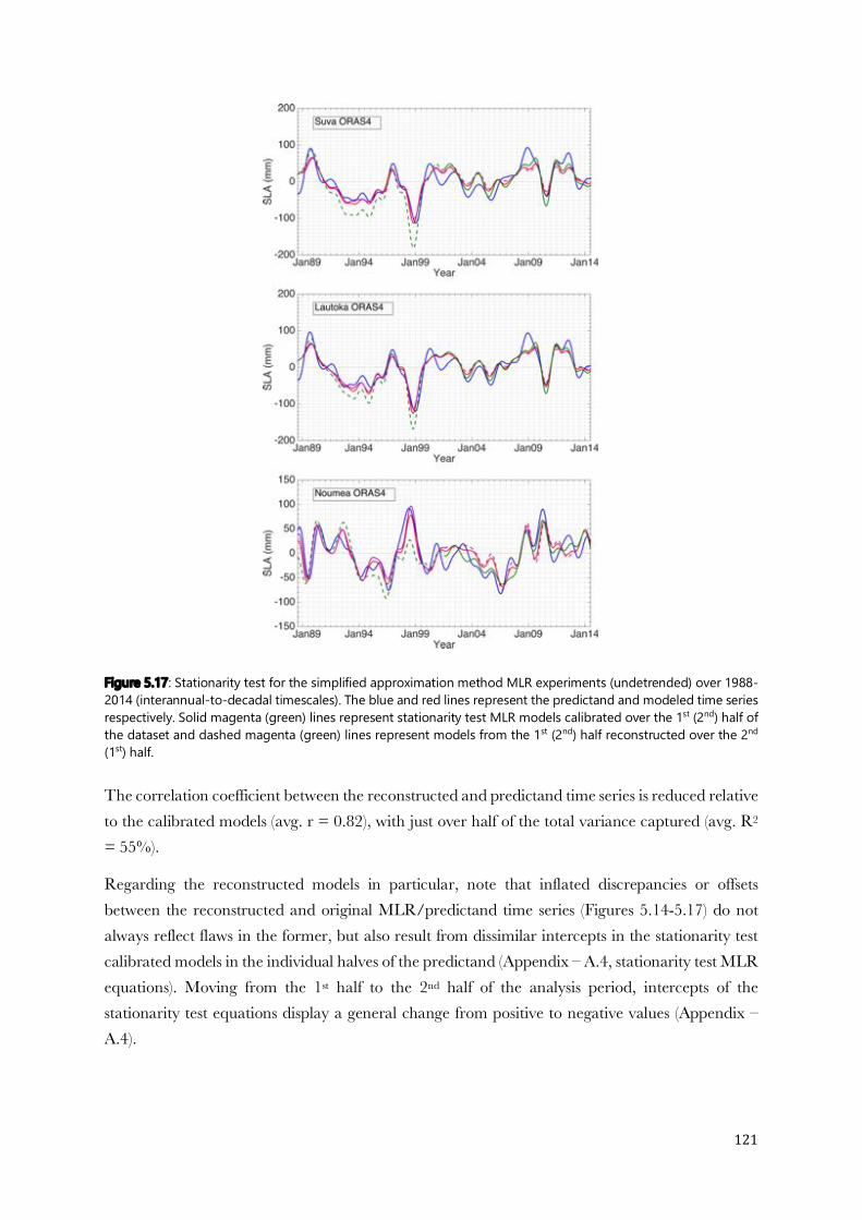
121

Figure 5.17: Stationarity test for the simplified approximation method MLR experiments (undetrended) over 1988-2014 (interannual-to-decadal timescales). The blue and red lines represent the predictand and modeled time series respectively. Solid magenta (green) lines represent stationarity test MLR models calibrated over the 1st (2nd) half of the dataset and dashed magenta (green) lines represent models from the 1st (2nd) half reconstructed over the 2nd (1st) half. The correlation coefficient between the reconstructed and predictand time series is reduced relative to the calibrated models (avg. r = 0.82), with just over half of the total variance captured (avg. R2 = 55%).

Regarding the reconstructed models in particular, note that inflated discrepancies or offsets between the reconstructed and original MLR/predictand time series (Figures 5.14-5.17) do not always reflect flaws in the former, but also result from dissimilar intercepts in the stationarity test calibrated models in the individual halves of the predictand (Appendix – A.4, stationarity test MLR equations). Moving from the 1st half to the 2nd half of the analysis period, intercepts of the stationarity test equations display a general change from positive to negative values (Appendix – A.4).

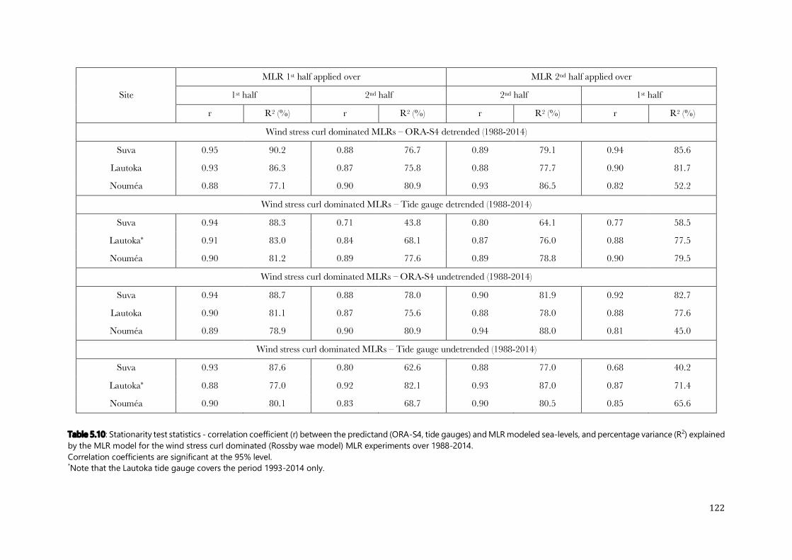
122

Site

MLR 1st half applied over MLR 2nd half applied over

1st half 2nd half 2nd half 1st half

r R2 (%) r R2 (%) r R2 (%) r R2 (%)

Wind stress curl dominated MLRs – ORA-S4 detrended (1988-2014)

Suva 0.95 90.2 0.88 76.7 0.89 79.1 0.94 85.6

Lautoka 0.93 86.3 0.87 75.8 0.88 77.7 0.90 81.7

Nouméa 0.88 77.1 0.90 80.9 0.93 86.5 0.82 52.2

Wind stress curl dominated MLRs – Tide gauge detrended (1988-2014)

Suva 0.94 88.3 0.71 43.8 0.80 64.1 0.77 58.5

Lautoka* 0.91 83.0 0.84 68.1 0.87 76.0 0.88 77.5

Nouméa 0.90 81.2 0.89 77.6 0.89 78.8 0.90 79.5

Wind stress curl dominated MLRs – ORA-S4 undetrended (1988-2014)

Suva 0.94 88.7 0.88 78.0 0.90 81.9 0.92 82.7

Lautoka 0.90 81.1 0.87 75.6 0.88 78.0 0.88 77.6

Nouméa 0.89 78.9 0.90 80.9 0.94 88.0 0.81 45.0

Wind stress curl dominated MLRs – Tide gauge undetrended (1988-2014)

Suva 0.93 87.6 0.80 62.6 0.88 77.0 0.68 40.2

Lautoka* 0.88 77.0 0.92 82.1 0.93 87.0 0.87 71.4

Nouméa 0.90 80.1 0.83 68.7 0.90 80.5 0.85 65.6

Table 5.10: Stationarity test statistics - correlation coefficient (r) between the predictand (ORA-S4, tide gauges) and MLR modeled sea-levels, and percentage variance (R2) explained by the MLR model for the wind stress curl dominated (Rossby wae model) MLR experiments over 1988-2014. Correlation coefficients are significant at the 95% level. *Note that the Lautoka tide gauge covers the period 1993-2014 only.

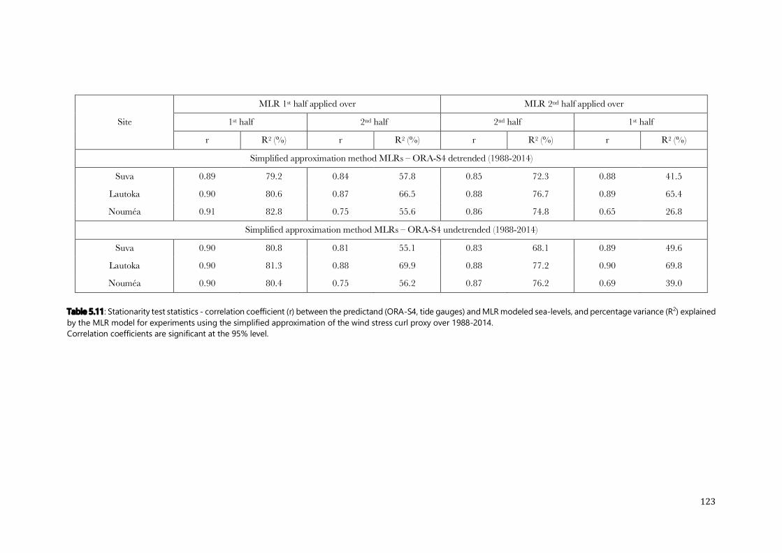
123

Table 5.11: Stationarity test statistics - correlation coefficient (r) between the predictand (ORA-S4, tide gauges) and MLR modeled sea-levels, and percentage variance (R2) explained by the MLR model for experiments using the simplified approximation of the wind stress curl proxy over 1988-2014. Correlation coefficients are significant at the 95% level.

Site

MLR 1st half applied over MLR 2nd half applied over

1st half 2nd half 2nd half 1st half

r R2 (%) r R2 (%) r R2 (%) r R2 (%)

Simplified approximation method MLRs – ORA-S4 detrended (1988-2014)

Suva 0.89 79.2 0.84 57.8 0.85 72.3 0.88 41.5

Lautoka 0.90 80.6 0.87 66.5 0.88 76.7 0.89 65.4

Nouméa 0.91 82.8 0.75 55.6 0.86 74.8 0.65 26.8

Simplified approximation method MLRs – ORA-S4 undetrended (1988-2014)

Suva 0.90 80.8 0.81 55.1 0.83 68.1 0.89 49.6

Lautoka 0.90 81.3 0.88 69.9 0.88 77.2 0.90 69.8

Nouméa 0.90 80.4 0.75 56.2 0.87 76.2 0.69 39.0

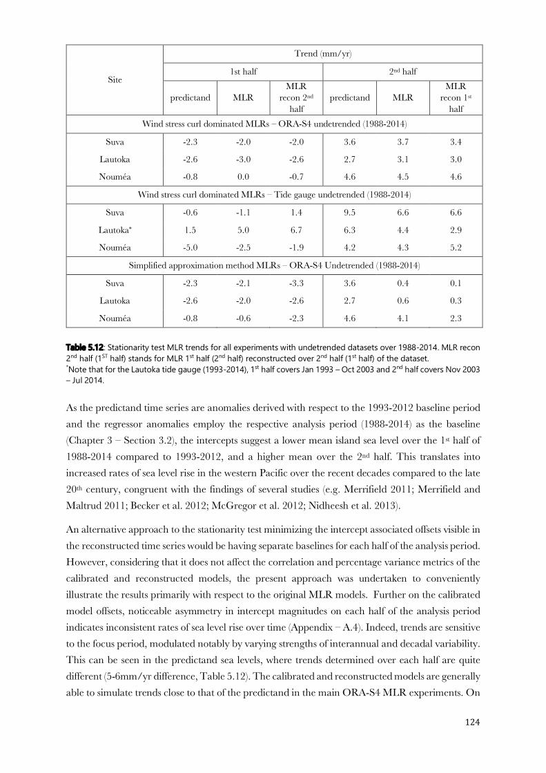
124

Table 5.12: Stationarity test MLR trends for all experiments with undetrended datasets over 1988-2014. MLR recon

2nd

half (1ST

half) stands for MLR 1st

half (2nd

half) reconstructed over 2nd

half (1st

half) of the dataset.

*

Note that for the Lautoka tide gauge (1993-2014), 1st

half covers Jan 1993 – Oct 2003 and 2nd

half covers Nov 2003

– Jul 2014.

As the predictand time series are anomalies derived with respect to the 1993-2012 baseline period and the regressor anomalies employ the respective analysis period (1988-2014) as the baseline (Chapter 3 – Section 3.2), the intercepts suggest a lower mean island sea level over the 1st half of 1988-2014 compared to 1993-2012, and a higher mean over the 2nd half. This translates into increased rates of sea level rise in the western Pacific over the recent decades compared to the late 20th century, congruent with the findings of several studies (e.g. Merrifield 2011; Merrifield and Maltrud 2011; Becker et al. 2012; McGregor et al. 2012; Nidheesh et al. 2013).

An alternative approach to the stationarity test minimizing the intercept associated offsets visible in the reconstructed time series would be having separate baselines for each half of the analysis period. However, considering that it does not affect the correlation and percentage variance metrics of the calibrated and reconstructed models, the present approach was undertaken to conveniently illustrate the results primarily with respect to the original MLR models. Further on the calibrated model offsets, noticeable asymmetry in intercept magnitudes on each half of the analysis period indicates inconsistent rates of sea level rise over time (Appendix – A.4). Indeed, trends are sensitive to the focus period, modulated notably by varying strengths of interannual and decadal variability. This can be seen in the predictand sea levels, where trends determined over each half are quite different (5-6mm/yr difference, Table 5.12). The calibrated and reconstructed models are generally able to simulate trends close to that of the predictand in the main ORA-S4 MLR experiments. On

Site

Trend (mm/yr)

1st half 2nd half

predictand MLR MLR

recon 2nd half

predictand MLR MLR

recon 1st half

Wind stress curl dominated MLRs – ORA-S4 undetrended (1988-2014)

Suva -2.3 -2.0 -2.0 3.6 3.7 3.4

Lautoka -2.6 -3.0 -2.6 2.7 3.1 3.0

Nouméa -0.8 0.0 -0.7 4.6 4.5 4.6


Suva -0.6 -1.1 1.4 9.5 6.6 6.6

Lautoka* 1.5 5.0 6.7 6.3 4.4 2.9

Nouméa -5.0 -2.5 -1.9 4.2 4.3 5.2

Simplified approximation method MLRs – ORA-S4 Undetrended (1988-2014)

Suva -2.3 -2.1 -3.3 3.6 0.4 0.1

Lautoka -2.6 -2.0 -2.6 2.7 0.6 0.3

Nouméa -0.8 -0.6 -2.3 4.6 4.1 2.3

125

the other hand, the calibrated and reconstructed models in the tide gauge based and the simplified approximation method MLR experiments display poor skill at reproducing the predictand trends (Table 5.12).

Overall, results of the stationarity test indicate that although some compromise in skill is generally expected when a calibrated MLR model is applied to a future scenario, it is still possible for reconstructed models to perform at levels similar to calibrated simulations. It can be inferred that the skill of the reconstructed model is predominantly determined by that of the calibrated model, depending on how accurately predictand-regressor relationships have been computed and how these relationships evolve over time. In the results presented, the main wind stress curl (Rossby wave model) dominated MLR models based on ORA-S4 predictands, which have been observed as the more robust of the calibrated models in the previous sections, produced reconstructions with the highest efficiency. Reconstructed models based on less robust MLR model formulations, such as those calibrated with tide gauge predictands or using the simplified approximation method, exhibit lower skill in comparison. In such cases, the resulting reconstruction is compromised by the culminated effects of a weaker MLR calibration in the original model, plus introduced uncertainties/incongruities from possible temporal variations in the predictand-regressor relationships. Nonetheless, even with the lowest performing reconstructed MLR models, correlation between the predictand and modeled sea levels remains relatively high, with a substantial proportion of variance reproduced.

5.4 Summary

Sea level time series for the study sites from reanalysis and altimetric sea level observations (absolute sea level) have high agreement with each other while tide gauge records (relative sea level) are affected by vertical land motion (subsidence, uplift) which can exacerbate or dampen sea level rise rates. Based on the current results, effects of vertical land motion are more pronounced at the Suva and Nouméa sites, and therefore, relative sea level trends must be interpreted with caution.

The preliminary MLR models exhibit very high similarity with the predictands, illustrating sea level as essentially a sum of steric and mass variations. The main MLR experiments are able to closely replicate the predictands (avg. r = 90%, avg. R2 = 80%), although model skill is slightly lower than the preceding steric plus mass MLRs, as expected. Given the consistency between ORA-S4 and regressor fields from ERA-Interim (used to force ocean model in the ORA-S4 reanalysis), performance of the MLR models using ORA-S4 predictand sea levels is overall higher compared to tide gauge-based models. Results from MLR models based on tide gauge predictands are further compromised by the effects of vertical land motion. While the role of the dominant wind stress curl regressor in the MLR model is plainly evident, the roles of the minor local wind stress and SST regressors remain ambiguous as results across the different experiments are inconsistent. The simplified approximation method MLR models showed lower skill than the main Rossby wave

126

model MLRs, as anticipated, yet were able to retain high correlation with the predictand and replicate the larger majority of the variance (avg. r = 0.88, avg. R2 = 78%).

Results of the stationarity test indicate that while some level of compromise can be expected when an MLR model calibrated over a particular period is applied to a future scenario, the reconstructed simulations can still retain skills comparable to the initial model. The skill of the reconstructed model, amongst other factors, depends foremost on the robustness of the calibration. Thus, MLR models which are not as robust, such as the those calibrated with tide gauge predictands, would not be able to produce very efficient reconstructions.

127

Chapter 6

Discussion 6.1 MLR model strengths and limitations ................................................... 129

6.1.1 Limitations inherent in the predictand datasets .................................................... 129 6.1.2 Limitations inherent in predictor selection ............................................................ 131

6.1.2.1 Inconsistency of regressor combinations across experiments ...................... 131 6.1.2.2 Representativeness of predictors ................................................................. 132

6.1.3 Limitations inherent to the MLR method ............................................................. 133 6.1.4 Basin-wide comparison of the thermosteric sea level and the Rossby wave modeled output.............................................................................................................................. 134 6.1.5 Simplified approximation method MLR models .................................................. 136

6.2 Stationarity ....................................................................................... 138

6.3 Comparison with ENSO, IPO indices .................................................... 140

6.4 Global warming and regional variability ............................................... 143

6.5 Comparison with other sea level downscaling experiments...................... 144

6.6 Practical concerns for future applications ............................................. 147

129

6. Discussion

The discussion chapter begins with an assessment of the MLR model strengths and limitations, weighing the different approaches/experiments presented. Possible constituents of the unexplained variance in the MLR modeled sea levels are discussed, and different sources of uncertainty identified. Additionally, a basin-wide comparison of thermosteric sea levels and the Rossby wave modeled output (wind-driven thermosteric component) across the Pacific is shown. Stationarity is discussed in the broader sense of statistical downscaling and the evolution of island sea levels and its components over time. The dominant regressor and predictand sea levels from the various experiments are then compared with the Niño 3.4 and the IPO indices, followed by discussion on interrelations between regional sea level rise in the Pacific and GMSL trends. The latter covers tropical Pacific sea level trend patterns, plus attributions, and discusses the challenges in robustly distinguishing natural and anthropogenic signatures in observations. The MLR model developed is then presented in the wider context of downscaling, comparing its success rates with other statistical and dynamical downscaling models for sea level. Finally, a list of practical concerns is discussed for applications in future projections.

6.1 MLR model strengths and limitations

6.1.1 Limitations inherent in the predictand and predictor datasets

The governing effect of wind stress curl on sea levels in the Pacific has been described in several studies (e.g. Carton et al. 2005; Kohl et al. 2007; Timmermann et al. 2010; McGregor et al. 2012; Nidheesh et al. 2013; Palanisamy et al 2015a). Based on this knowledge, a multiple linear regression model combining regional and local atmospheric/oceanic variables for island sea levels in the western Pacific was developed, using wind stress curl as the dominant regressor.

Sea level change can be interpreted as a change in the volume of the water column, resulting from density (steric) and/or mass changes. The preliminary set of MLR experiments using only predictors for the steric and mass contribution to sea level changes aimed at verifying that the MLR model behaved as expected in this simplified framework, before moving onto the main wind-stress curl dominated set of MLR experiments. Amongst the main outcomes from the preliminary MLR models was the inclusion of mass change as a significant regressor in the stepwise selection for the undetrended experiments, evidencing the growing contribution of mass to rising sea levels as warming continues. The results revealed mass comprising a relatively small yet significant proportion of island sea level variance (R2 = 1-2%), which is expected to augment as warming trends persist in future.

In the main MLR experiments, a linear Rossby wave model was employed to simulate wind stress curl forced modulations to the pycnocline depth, which translate into thermosteric variations and resultant sea level change. The MLR models produced high correlations with the predictand sea

130

levels and successfully reproduced a large majority of the variance (avg. R2 = 80%). Comparing similar models calibrated with ORA-S4 and with tide gauge sea levels, MLR models using ORA-S4 sea levels as predictands produced island sea level time series bearing higher resemblance to the predictands than the MLR models using tide gauge data as predictands. This is congruent with the added consistency between the predictand and regressor fields in MLR experiments using ORA-S4 sea levels as predictands (e.g. ERA-Interim fields used to force ORA-S4; Chapters 3, 5).

With the tide gauge based predictands being adjusted for missing values only, and not for biases introduced by vertical land motion (subsidence, uplift) acting upon the study sites over time, accuracy of the MLR models was compromised to some extent in calibrating a best fit on a biased time series. As there were two sets of predictands for each site – reanalysis and in situ, serving as a platform to draw analytical comparison between the calibrated models, there was not much emphasis on correcting for biases in the latter. Rather, the reanalysis sea levels, together with altimetric observations, were used to identify and source errors/biases affecting the tide gauge records from existing literature before proceeding to the MLR models. Resulting limitations in the tide gauge based MLR models relative to the corresponding ORA-S4 models illustrate how any bias in the predictand dataset is projected onto the model calibration. Thus, if a similar downscaling approach is employed to extract information for implementing adaptation or risk minimization projects on ground, it is critical that in situ data are pre-examined and systematically corrected for suspected bias. The same degree of caution has to be exercised in selecting regressor datasets as well. It is worth acknowledging that each reanalysis product also exhibits individual bias and no single product has exact agreement with all satellite-derived observations (e.g. Chaudhuri et al. 2013; Lu et al. 2013).

For example, in a study linking regional sea level trends to the intensification of Pacific trade winds by Merrifield and Maltrud 2011, wind stress forcing from ECMWF’s ORA-S3 (Balmaseda et al. 2008) was used in a general circulation model to successfully replicate the observed sea level trend signature in the Pacific basin. The simulated sea level trends were not as realistic when the model was forced with NCAR/NCEP (Kalnay et al. 1996) wind stress, fields as the product does not incorporate scatterometer winds, unlike ORA-S3. McGregor et al. 2012, using a more extensive set of wind stress products, further illustrated that the choice of the dataset is relatively unimportant when focusing on high-frequency variability, but is crucial for assessing long-term linear trends in sea level. Similarly, the GECCO2 ocean synthesis has a good representation of general large-scale variability but has pronounced biases along the Antarctic Circumpolar Current (ACC) in the Southern Ocean (Köhl 2015; Scharffenberg et al. 2017). In ORA-S4, there are large uncertainties in the starting two decades of the product (1960s-1970s) and an underestimation of the Atlantic Meridional Circulation (AMOC) (Balmaseda et al. 2013a; 2013b). As such, any modeled, reconstructed, or reanalysis dataset can have overall good simulation skills but typically possess certain regional, temporal, or climate/ocean circulation feature related biases. Thus, for similar downscaling or evaluation studies covering a particular focus area, an optimum set of data products

131

should be selected based on performance regionally and not only skill at reproducing general large-scale patterns/variability. In other words, as demonstrated by the results of this study, an integral component of a robust statistical model is a robust calibration dataset.

6.1.2 Limitations inherent in predictor selection

6.1.2.1 Inconsistency of selected regressor combinations

While resemblance between the predictand and the modeled sea levels was overall high in the main set of MLR experiments, especially when considering the more efficient ORA-S4 based models, the MLR model was less robust in terms of consistency in significant regressor combinations across the various experiments. Across all of the main experiments, the wind stress curl (thermosteric proxy) and the local halosteric component were the only two regressors to remain significant throughout. However, there was no discernible pattern in the selection of the other regressors for any particular site from the detrended to the undetrended experiments, or between corresponding experiments conducted with ORA-S4 and with tide gauge predictands, or even for sites with high proximity to each other (Fiji sites – Suva, Lautoka). The continual selection of the wind stress curl (thermosteric proxy) and halosteric regressors is the MLR model representation of island sea level variations as essentially steric, where the dominating thermosteric component is governed by dynamic regional processes. Excluding a fractional contribution from the deeper ocean (Chapter 4 – Section 4.2), the remaining variability in island sea level is mostly controlled by local processes, including wind set-up and surface buoyancy fluxes. Although the MLR model attempts to incorporate the remaining local component through wind stress (zonal/meridional) and SST, the absence of a consistent regressor combination could suggest significant degree of covariance between the non-dominant regressors when they act in concert, reinforcing or compensating each other (coupled interaction). It could also indicate weak relationships with the predictand, whereby the strength of the association is unsteady over time and overall insufficient to secure selection in the stepwise regression. Thus, perceiving the purpose of the MLR model as two-fold, where the aim is not only to produce a closest possible simulation of the predictand but to also robustly identify predictand-regressor relationships, the latter was not fully achieved.

Further on the local regressors, a possibly relevant aspect could be how robustly the wind stress and SST variables are represented as potential predictors (MLR input variables). Here, some degree of correlation may still remain amongst the isolated regressors from a methodology limitation, whereby the proportion of island sea level represented only by the dominant thermosteric proxy is removed from the predictand before the other regressors are selected (Chapter 3 – Sections 3.6.2 and 3.6.3). While the issue of covariance amongst the final set of regressor time series is counteracted with the use of a stepwise regression function, the variables aside from the dominant are all selected on basis of correlation with the remaining proportion of sea level without much regard to covariance that may remain between them (e.g. between surface freshwater and heat

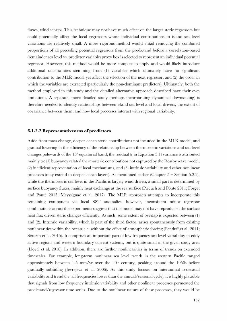
132

fluxes, wind set-up). This technique may not have much effect on the larger steric regressors but could potentially affect the local regressors whose individual contributions to island sea level variations are relatively small. A more rigorous method would entail removing the combined proportions of all preceding potential regressors from the predictand before a correlation-based (remainder sea level vs. predictor variable) proxy box is selected to represent an individual potential regressor. However, this method would be more complex to apply and would likely introduce additional uncertainties stemming from (1) variables which ultimately have no significant contribution to the MLR model yet affect the selection of the next regressor, and (2) the order in which the variables are extracted (particularly the non-dominant predictors). Ultimately, both the method employed in this study and the detailed alternative approach described have their own limitations. A separate, more detailed study (perhaps incorporating dynamical downscaling) is therefore needed to identify relationships between island sea level and local drivers, the extent of covariance between them, and how local processes interact with regional variability.

6.1.2.2 Representativeness of predictors

Aside from mass change, deeper ocean steric contributions not included in the MLR model, and gradual lowering in the efficiency of the relationship between thermosteric variations and sea level changes polewards of the 15º equatorial band, the residual (ε in Equation 3.1) variance is attributed mainly to: (1) buoyancy related thermosteric contributions not captured by the Rossby wave model, (2) inefficient representation of local mechanisms, and (3) intrinsic variability and other nonlinear processes (may extend to deeper ocean layers). As mentioned earlier (Chapter 5 – Section 5.2.2), while the thermosteric sea level in the Pacific is largely wind driven, a small part is determined by surface buoyancy fluxes, mainly heat exchange at the sea surface (Piecuch and Ponte 2011; Forget and Ponte 2015; Meyssignac et al. 2017). The MLR approach attempts to incorporate this remaining component via local SST anomalies, however, inconsistent minor regressor combinations across the experiments suggests that the model may not have reproduced the surface heat flux driven steric changes efficiently. As such, some extent of overlap is expected between (1) and (2). Intrinsic variability, which is part of the third factor, arises spontaneously from existing nonlinearities within the ocean, i.e. without the effect of atmospheric forcing (Penduff et al. 2011; Sérazin et al. 2015). It comprises an important part of low frequency sea level variability in eddy active regions and western boundary current systems, but is quite small in the given study area (Llovel et al. 2018). In addition, there are further nonlinearities in terms of trends on extended timescales. For example, long-term nonlinear sea level trends in the western Pacific ranged approximately between 1-5 mm/yr over the 20th century, peaking around the 1950s before gradually subsiding (Jevrejeva et al. 2006). As this study focuses on interannual-to-decadal variability and trend (i.e. all frequencies lower than the annual/seasonal cycle), it is highly plausible that signals from low frequency intrinsic variability and other nonlinear processes permeated the predictand/regressor time series. Due to the nonlinear nature of these processes, they would be

133

obscured in the linear regression model and thus most likely contribute a small part of the residual variance from the MLR model.

6.1.3 Limitations inherent to the MLR method

In addition to the specifics and limitations of the statistical model formulation discussed above, the scope of the linear regression technique itself should be noted. Uncaptured nonlinear processes aside, the MLR method computes fixed coefficients to describe the overall relationship between the predictand and regressor over a given temporal span. This translates into a static relationship between the two variables in the calibration process. In reality, however, the strength of the relation varies over time, often exhibiting variability at decadal timescales (Han et al. 2017). Consider for example, the case of the PDO; while it is the leading empirical mode in the North Pacific basin on decadal timescales, it is not entirely deemed as a single physical mode of climate variability but a combination of different processes as they interact with each other (Han et al. 2017). These processes are (1) Aleutian low-associated variability from stochastic weather noise and remote forcing from the tropics (mostly ENSO), (2) ocean memory, and (3) decadal variability of the Kuroshio-Oyashio currents generated by westward propagation of Rossby waves (Newman et al. 2003; 2016). Thus, different processes may dominate PDO during different events, with decadal variability associated with winds, SST, heat/freshwater fluxes manifesting in sea level at altered strengths.

Limitations with the linear regression technique have been documented in other sea level studies as well. Assessing the residual sea level in the Pacific Ocean after removing the decadal variability signal via EOFs, Hamlington et al. 2014 and Han et al. 2014 link the pattern to anthropogenic warming. However, a following study by Palanisamy et al. 2015b using linear regression found nonlinear ENSO related variability in the aforementioned residual, indicating that neither EOFs nor linear regression are able to completely remove internal variability signatures from sea level (Marcos et al. 2017). For island sea levels, however, note that such nonlinearities would generally be quite small and remain part of the unmodeled residual.

Overall, acknowledging the unmodeled residual and uncertainties in robustly representing local processes, the MLR model’s best skill is grounded in its ability to simulate the governing regional driver – wind stress curl anomalies driving the dominant thermosteric component in the tropical zone. As dominant regressor, the wind stress curl proxy alone is able to replicate a vast majority of island sea level variance (ORA-S4 experiments R2 = 70-75%, tide gauge experiments R2 = 40-72%; Appendix A.2), encapsulating all major interannual-to-decadal signals (Chapter 5 – Section 5.2.2). With the ORA-S4 predictand data sets, the variance percentages replicated by the MLR model and by the wind stress curl proxy are on comparable scales (~ 10% difference on avg.; compare Chapter 5 – Table 5.5 and Appendix A.2). Indeed, the wind driven steric variation plays a critical role in climate and oceanic changes across the region and can be used to successfully

134

model the timing of ENSO and decadal variability (Hill et al. 2011; Holbrook et al. 2011; Qiu and Chen 2006; Sasaki et al. 2008). Given that practical applications for interannual-to-decadal scale variability projections would typically be based on long-term mean sea levels, unlike for a forecast model, the MLR model would still be able to provide highly valuable information despite the limitations mentioned since a maximum range can easily be extrapolated from the modeled time series (or even the dominant regressor). I.e. a good estimate of island sea level variations can be obtained with information of the regional driver. This is the focus of the next two subsections.

6.1.4 Basin-wide comparison of the thermosteric sea level and the Rossby wave modeled output

The use of a linear Rossby wave model converting wind stress vectors into pycnocline (thermocline) depth anomalies and resultant thermosteric change was an integral component of the experiment design (Chapter 3 – Section 3.5). This section presents a basin-wide comparison of the thermosteric sea level and the Rossby wave modeled thermosteric change, both of which have been correlated with the island sea levels for each site (Figure 6.1).

On the western side of the Pacific, the thermosteric sea level and the Rossby wave modeled thermosteric change exhibit close resemblance to each other, demonstrating the former as essentially wind driven (Figure 6.1). They also portray the slowly varying, large-scale signature of the thermosteric component closer to the equatorial region. Towards the eastern end of the basin, for the Fiji sites, correlations between island sea levels and the thermosteric component become negative (Figure 6.1 – a, c), consistent with Walker circulation dynamics, where the coupled ocean-atmosphere pile-up warm waters in the western tropical Pacific as cold, nutrient rich waters upwell in the east (Gill 1982; Lau and Yang 2015; Chang and Zebiak 2015). The basin-wide pattern also corresponds to the signature east-west dipole in recent sea level trends in the Pacific (McGregor et al. 2012; Becker et al. 2012; Nidheesh et al. 2013; Stammer et al. 2013; Palanisamy et al. 2015a, Marcos et al. 2017).

Correlations between island sea levels and the Rossby wave modeled thermosteric change remain positive, but decline notably in magnitude moving eastwards (Figure 6.1 – b, d). The contrast between the two (a, c and b, d) strongly indicates differences between driving mechanisms for steric change at the western and eastern ends of the tropical Pacific. Indeed, while sea levels in the western Pacific are predominated by wind-driven westward propagation of Rossby waves, sea levels in the eastern Pacific vary primarily under the influence of the eastern boundary forcing, with some contribution from local surface heat fluxes and Ekman pumping (Fu and Qiu 2002; Qiu and Chen 2006; Lu et al. 2013).

The case of Nouméa, on the other hand, is quite different from Fiji’s as it lies along the margins of spatial signatures characteristic of the acting climate modes in the southwest Pacific (Figure 6.1 – e,

135

Figure 6.1: Island sea level for the study sites (ORA-S4) correlated with the basin-wide thermosteric sea level (a, c,

e) and the Rossby wave modeled thermosteric change (b, d, f) at interannual-to-decadal timescales over 1988-2014

(undetrended).

f). Thus, as observed throughout the results of this study and of several others (e.g. Wang et al. 2000; Lee and Fukumori 2003; Sasaki et al. 2008; Ganachaud et al. 2011; Forget and Ponte 2015), sea level variations at Nouméa and Fiji appear somewhat opposite in phasing. In addition to the east-west dipole pattern (interannual variability related), Figure 6.1 – e also highlights the lower portion of the other distinctive sea level trend signature in the Pacific (decadal variability related), which is the broad-scale V-shaped positive trend pattern spreading from about 30°–50° N in the central

136

basin to the western equatorial Pacific and then to 30°–50° S in the central–eastern basin (England et al. 2014; Hamlington et al. 2014; Han et al. 2014; Palanisamy et al. 2015a; Marcos et al. 2017) (Chapter 2 – Section 2.16).

Correlation with the Rossby wave determined thermosteric sea level at Nouméa is somewhat weaker relative to the Fiji sites, with the region of maximum values not completely extending to New Caledonia (Figure 6.1 – f). This is consistent with a lower Rossby wave energy moving away from the tropical zone, which translates into a reduced level of thermosteric change emanating from modulations to the thermocline depth. Wind driven interannual and longer-term steric sea level variations, including the trend, in fact, have been found to be largest within 15° of the equator (e.g. White at al. 1985; Rebert et al. 1985; Palanisamy et al. 2015a). Polewards beyond this zone, the thermocline starts weakening and the ocean no longer resembles a two-layer system. The relationship between the dynamic steric component and sea level has been found to be optimum where the ocean most closely bears resemblance to a two-layer system, which ideally has a single baroclinic mode with maximum vertical displacements at the interface (Rebert et al. 1985; McGregor et al. 2012). Large scale baroclinic waves are furthermore observed at low latitudes only, where the ratio of the crossing time to the unstable growth time (baroclinic instability) is small; the critical latitude is about 20º (Isachsen et al. 2007). Thus, the combined effect on model precision at the Fiji sites, which lie between 17-18º S, would be lower than that at Nouméa, which lies at 22º S. On the other hand, surface buoyancy induced steric variations, particularly heat fluxes, are relatively higher at Nouméa (Piecuch and Ponte 2011; Meyssignac et al. 2017); this is congruent with the continual selection of SST as a significant regressor in all of the MLR experiments for Nouméa (Chapter 5 – Sections 5.2.2, 5.2.3). Similarly, contributions from low frequency intrinsic ocean variability around Nouméa are also higher in comparison to Fiji (Penduff et al. 2011; Sérazin et al. 2015).

6.1.5 Simplified approximation method MLR models

The simplified approximation method MLR experiments omitted the use of a Rossby wave model and estimated the dominant regressor as remotely located and leading wind stress curl anomalies eastwards of the study site via a correlation-based selection. In essence, the approximation method attempted to test if and the extent to which wind stress curl anomalies per se could be used to obtain some level of viable information on island sea level variations.

In the approximation method, the regression function attempts to calibrate a directly proportional relationship between proxy box wind stress curl anomalies and island sea level. Analyzing the results, this estimate can in fact be identified as the main limitation in the approximation method since the relationship between the two variables is more complex.

137

The mechanism responsible for conveying wind forcing into sea level are baroclinic Rossby waves, which have spatially varying speeds determined to a great extent by the level of stratification, change in Coriolis parameter with latitude, and the Rossby radius of deformation (e.g. White et al. 1985; Chelton et al. 1998; Holbrook et al. 2011; McGregor et al. 2012; Kessler and Cravatte 2013b) (see Chapter 3 – Equation 3.3). An attempt to define a relationship between wind stress curl and sea level using the approximation technique overlooks these deterministic parameters thereby resulting in a compromised estimate.

The approximation approach used a leading time of 6 months for wind stress curl (i.e. sea level lagging), which was determined heuristically from a set of correlations performed with island sea level from consecutively increasing lead periods from 1 to 12 months. At the 6-month estimate, the approximate speeds of the propagating Rossby waves (cr) towards Fiji and Nouméa, based on the distance between the proxy boxes and the study sites, equated to 0.19 m/s and 0.12 m/s respectively. These values are on a comparable range with those in existing literature, e.g. White et al. 1985, Chelton and Schlax 1996, Palanisamy et al. 2015a, and when using the relationship between the long Rossby wave speed (cr) and the internal long gravity wave speed (c) (see Chapter 3 – Equation 3.3), they yield a first baroclinic gravity wave speed of 2.8 m/s, in agreement with reported values in the focus area (Chelton et al. 1998). Propagation speeds in the western basin are higher compared to the eastern as a result of variations in stratification, which is much stronger at the western end. For example, the Rossby wave speed in the equatorial Pacific increases from about 2.2 m/s off the coast of Ecuador to about 3 m/s near the dateline (e.g. Chelton et al. 1988; Lu et al. 2013). Zonal averages are therefore often used to describe propagation speeds or determine east-to-west transit periods. At the aforementioned speeds, the Rossby waves would take 3-4 years to cross the Pacific basin from its eastern boundary before reaching Fiji and 5-6 years before reaching Nouméa (Qiu and Chen 2006), which would be the duration for the associated sea level changes to manifest at the islands. A 6-month lead period thus represents a Rossby wave on the ending segment of its cross-basin transit.

Compared to the main experiments employing the Rossby wave model, correlation between the dominant regressor and the thermosteric sea level reduces from high to a medium range, and the percentage variance of the predictand replicated declines from majority to less than 50% (Chapter 6– Table 6.8). These statistics lie within a similar range as those between the dominant regressor and the predictand for the main and the approximation method MLR experiments (Appendix – A.2) as the predictand is dominated by the thermosteric component.

A potentially compensating advantage of the approximation method MLR models, on the other hand, is consistency in the selected set of regressors in the calibrated model, which is absent in the main Rossby wave model experiments. This feature certainly does not balance out the overall variance lost in using the wind stress curl proxy box over the Rossby wave model, but is a key element for robustness in any regression model.

138

Despite these limitations, the approximation method is able to model sea levels with overall high correlation with the predictand and explaining the larger majority of the predictand variance (70-80%, ~ 10%< main MLR models) (Chapter 6 – Table 6.5), optimizing the MLR technique upon the limited skill of the dominant regressor and a more representative set of local regressors. However, while the approximation method MLR models exhibit this level of skill, their limitations become more obvious in the stationarity tests (Chapter 5 – Section 5.3). Thus, other than for comparative purposes, the use of a Rossby wave model is always recommended for similar studies.

6.2 Stationarity

Results from the stationarity tests illustrated the MLR models’ capacity to retain fair skill when being applied to a different period from the one used for calibration (Chapter 5 – Section 5.3). As the study focused on interannual-to-decadal scale sea level variability, the stationarity was test was conducted on a dataset spanning just above the minimum two decades required (26 years – 1988-2014). Given a longer duration of the predictand/regressor datasets spanning several decades, it would have been possible to perform a more robust test of stationarity.

Aside from possible evolutions in predictand-regressor relationships over time, model stationarity depends on the robustness of the calibration between the predictand/regressor datasets. The reconstructions also demonstrated particular sensitivity to trends, which vary with the time frame selected and acting climate modes, and determine offsets between the calibrated and reconstructed time series (applicable only when temporal mean over the calibration period is not equal to zero).

This section discusses the concept of stationarity in the broader sense of statistical downscaling, particularly with regards to sea level rise in the context of its components, plus their evolution over time. Note that the discussion does not cover vertical land motion (both natural and anthropogenic), which may be aptly incorporated as a correction to the modeled time series for future projections.

In this study, the MLR model represents (1) the deterministic regional component and (2) relatively minor local drivers. The rising GMSL, which is the product of thermal expansion and mass change, is effectively removed from the MLR by removing the GMSL trend from the predictand time series (Chapter 3 – Section 3.6.2.1). Assuming little-to-insignificant adjustments in predictand-regressor relationships over extended periods (decadal-to-century scale), a robust model can be presumed to simulate the combined regionally and locally defined part of island sea level changes with practically the same success rates for future scenarios. However, land-ice mass loss (from glaciers and ice sheets) is projected to increase continuously in response to ongoing warming trajectories. Thermal expansion is also committed to continue for centuries, and is projected to remain the dominant contributor to GMSL rise over the 21st century (e.g. Church et al. 2013, Golledge et al. 2015). However, unlike for the barystatic component, the regional signatures of steric component are heterogeneous and may overlap with regional variability (e.g. Fukumori and Wang 2013; Slangen

139

et al. 2014b; Forget and Ponte 2015). As the island sea levels result from the global, regional and local components of sea level changes and their interactions, an increasing GMSL would explain a larger proportion of total sea level, and the relative proportion of the combined regional and local components to total sea level is set to decline accordingly. In other words, an MLR model calibrated robustly over a given timespan at the start of the 21st century and then applied towards the end of the century, even when hypothetically retaining the maximum of its simulation skills, would produce a simulation with a reduced percentage of explained variance of the total island sea level (including the GMSL). The MLR model would be simulating precisely what it has been designed to, and the time-evolution of unrepresented components should not break the stationarity hypothesis of the model. Hence, if the only significant change in the predictand over two periods is the relative proportion of the global component, the modeled (regional + local) plus adjusted global component should remain more or less equivalent.

Regarding the barystatic component in particular, its relatively uniform signature and predictable fingerprint in future sea level projections (Bamber and Riva 2010; Slangen et al 2014a) make it an unsophisticated adjustment to apply to the MLR model simulated sea level output for future scenarios (as an a-posteriori addition). For the steric component of the global mean, the adjustment may be more difficult to apply due to its uneven signature and overlap with the regional climate modes.

The other aspect to consider with regards to stationarity is nonlinearities arising within the ocean over extended periods. The concept of nonlinearities in the ocean is quite broad, with manifestations in different forms or features pertaining to sea level, and often with overlaps amongst the constituents. Non-linearities can occur, for example, in the thermosteric component (e.g. Rugenstein et al. 2016; Yin et al. 2010, as well as in variations in strengths of individual regressor-predictand relationships (Han et al. 2017), or in the proportionate mechanisms inducing sea level change during different ENSO and decadal variability events (Moon et al. 2015; Han et al. 2017). Note that the latter two may also be perceived as limitations of the linear regression technique itself (Section 6.1).

Of special importance is the evolution of thermosteric sea level over time and depth. While ocean heat uptake dominates the sequestration of the planet’s excess heat due to global warming (e.g. Church et al. 2011), the perturbed ocean can take up to millennia to reach a full equilibrium (Rhein et al. 2013; Goosse 2015). On timescales of centuries to millennia, thermal expansion becomes nonlinearly dependent on forcing levels and surface warming. Nonlinearity results from (1) the nonlinearity of the equation of state, whereby the expansion coefficient of seawater increases with temperature and lowered pressure (e.g. Vallis et al. 2005; Palter et al. 2014), (2) the transient effects of higher heat uptake with time, but with simultaneous transfer of larger fractions into the deep ocean layers, where thermal expansion is lesser (e.g. Boé et al. 2009; Winton et al. 2010; Rose and Rayborn 2016), and (3) forcing level and ocean circulation/mixing dependent heat uptake (e.g. Rugenstein et al. 2016; Kuhlbrodt and Gregory 2012 ). Consequently, it becomes increasingly

140

complex to distinguish short and long-term heat uptake patterns. Heat uptake by the ocean is confined primarily to the upper ocean, however, the fraction that penetrates to the deeper layers can comprise notable proportions of the total amplitude of thermosteric change, visible within decades of the perturbation (Kuhlbrodt and Gregory 2012; Marshall et al. 2015).

Elaborating further on factor (2) from above, while historical and present day steric sea level rise is essentially from the upper 1000 m of the ocean, studies on future sea level projections have found significantly higher contributions from the layers below, which become quite distinct towards the 2nd half of the 21st century (Yin et al. 2010; Yin 2012). Considering the formulation of a statistical model of the type presented in this study, the ocean layers used for the calibration and future projection models thus becomes an important matter. So while the present MLR models have been calibrated with steric components from the upper 700 m of the ocean (Chapter 4 – Section 4.2), the same models applied in downscaling future sea level projections may need to incorporate deeper layers to simulate the same proportion of variance, or acknowledge a higher contribution from the unrepresented layers.

In summary, the evolution of the represented components of sea level relative to each other (e.g. local, regional, global) over time is a key factor in determining the success rate of the MLR model for future projections. Even if a skillful model retains its robustness for simulating, say the regional and local components, the total percentage variance simulated would be lower if the global mean undergoes a comparative marked increase. In addition, particularly considering nonlinearities in the thermosteric expansion of sea water, it should be noted that the MLR model designed here is intended for applications typically in decadal-to-century scale projections. Depending on the intended use, it is critical to separate decadal and century scale GCM simulations which would function as input datasets for the statistical model (different GCM runs for different timescales). Similarly, depth-specific contributions to the total steric rise over these time frames should be adjusted for accordingly. As the nonlinearities discussed are beyond the scope of the MLR model, it is recommended that time and region dependent (e.g. Dewar et al. 2003) nonlinearity estimates, even in the form of uncertainty ranges, are incorporated in the downscaled sea level time series for more reliable projections.

6.3 Comparison with ENSO, IPO indices

ENSO and IPO/PDO are the leading modes of climate variability in the Pacific region on interannual and decadal timescales respectively (Chapter 2 – Section 2.1.6). While these frequencies are of focus in the present study, the primary analysis does not separately examine ENSO and IPO/PDO in the context of the MLR model, concentrating rather on the manifestation of interannual-to-decadal variability in regional wind forcing (leading driver). This section presents a correlation analysis between the Niño 3.4 (ENSO), IPO indices and (1) the dominant wind stress

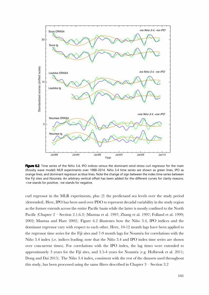
141

Figure 6.2: Time series of the Niño 3.4, IPO indices versus the dominant wind stress curl regressor for the main

(Rossby wave model) MLR experiments over 1988-2014. Niño 3.4 time series are shown as green lines, IPO as

orange lines, and dominant regressor as blue lines. Note the change of sign between the index time series between

the Fiji sites and Nouméa. An arbitrary vertical offset has been added for the different curves for clarity reasons.

+ive stands for positive, -ive stands for negative.

curl regressor in the MLR experiments, plus (2) the predictand sea levels over the study period (detrended). Here, IPO has been used over PDO to represent decadal variability in the study region as the former extends across the entire Pacific basin while the latter is mostly confined to the North Pacific (Chapter 2 – Section 2.1.6.3) (Mantua et al. 1997; Zhang et al. 1997; Folland et al. 1999; 2002; Mantua and Hare 2002). Figure 6.2 illustrates how the Niño 3.4, IPO indices and the dominant regressor vary with respect to each other. Here, 10-12 month lags have been applied to the regressor time series for the Fiji sites and 7-9 month lags for Nouméa for correlations with the Niño 3.4 index (i.e. indices leading; note that the Niño 3.4 and IPO index time series are shown over concurrent times). For correlations with the IPO index, the lag times were extended to approximately 3 years for the Fiji sites, and 3.5-4 years for Nouméa (e.g. Holbrook et al. 2011; Dong and Dai 2015). The Niño 3.4 index, consistent with the rest of the datasets used throughout this study, has been processed using the same filters described in Chapter 3 – Section 3.2

142

Site r - Niño 3.4 index vs. r - IPO index vs.

Dominant regressor Island sea level Dominant

regressor Island sea level

Wind stress curl dominated MLRs – ORA-S4

Suva -0.74 -0.74 -0.50 -0.28

Lautoka -0.72 -0.71 -0.52 -0.26

Nouméa 0.44 0.36 0.41 0.40

Wind stress curl dominated MLRs – Tide gauge

Suva -0.74 -0.55 -0.53 0.01

Lautoka* -0.74 -0.66 0.25 -0.14

Nouméa 0.53 0.22 0.33 0.32

Table 6.1: Correlation coefficient (r) between the Niño 3.4, IPO indices and the (1) dominant wind stress curl

regressor, (2) island sea level for the main (Rossby wave model) MLR experiments over 1988-2014.

Correlation coefficients are significant at the 95% level.

*Note that the Lautoka tide gauge covers the period 1993-2014 only

(detrended, deseasonalized, 1.2 year low-pass filtered), preserving interannual-to-decadal scale variability.

For the IPO index, the cut-off frequency in the low-pass filter was changed to 13 years to isolate decadal-to-multidecadal scale variability (e.g. Power et al. 1999; Folland et al. 2002; Henley et al. 2015). For convenience of illustration, the indices time series have been inversed to match the regressor’s where appropriate (Fiji sites; note aforementioned opposite phasing between Fiji and Nouméa sea levels).

Table 6.1 provides correlation coefficients between the indices and regressor time series presented in Figure 6.2, as well as island sea level. At common frequencies, the Niño 3.4 and IPO indices are highly correlated with each other (r = 0.92-0.95) (e.g. Zhang and Church 2012), with some extent of modulation of ENSO events by decadal variability (Power et al. 1999; 2006; Verdon and Franks 2006).

Consistent with ENSO signatures in the western Pacific (Chapter 2 – Section 2.1.6.2), the Niño 3.4 index has a relatively strong negative correlation with island sea levels at Fiji (Table 6.1 – ORA-S4). The Nouméa time series, whose sea level patterns are in opposite phasing to Fiji’s, has a low positive correlation with the Niño 3.4 index. Correlations with tide gauge sea levels and the simplified approximation method wind stress curl proxies, produce comparatively lower coefficient values than the others, as expected (Chapter 6).

Where both the island sea levels and the dominant regressor datasets are known to be more robust (e.g. main ORA-S4 experiments), the Niño 3.4/island sea level and Niño 3.4/dominant regressor

143

correlation coefficients are similar (Table 6.1), indicating corresponding responses in wind forcing and in sea level to the phases of ENSO.

In regards to possible modulating effects of IPO on the effects of ENSO, as has been observed for variables such as rainfall and sea level in certain areas (e.g. Power et al. 1999; Moon et al. 2015), the present results do not reveal any discernible patterns between the magnitude of the ENSO influence on island sea level and the phases of IPO (Figure 6.2). Moon et al. 2015, for example, demonstrated the modulated behavior of tropical Pacific sea levels under interannual and decadal oscillations. However, their results reflect the averaged regional response and not necessarily sea level at individual stations, especially those outside the 15º equatorial band.

Correlation values with the IPO index are generally much lower in comparison to Niño 3.4, especially for Fiji sites (Table 6.1). Yet, the IPO statistics are limited by the length of the time series for analyzing decadal variability (26 years), as is the determination of precise lag periods.

Additionally, it is important to note that the statistics obtained in Table 6.1 are sensitive to the datasets used as well. As observed earlier with the MLR results (Chapter 5 – Section 5.2), evaluation metrics are generally higher when there is underlying consistency between the datasets involved (ORA-S4 predictands), and are compromised in the presence of biased datasets (e.g. tide gauge records for Suva and Nouméa – Chapter 5 – Section 5.1) or inefficient proxies.

6.4 Global warming and regional variability

Most sea level studies focusing on regional or local scales effectively remove the GMSL in order to separate the different signals acting at these scales (e.g. Timmerman et al. 2010; Suzuki and Ishii 2011; Meyssignac et al. 2012; Palanisamy et al. 2015a, b; Sterlini et al. 2016; Han et al. 2017). The same practice has been adopted in this study as well; the MLR model has a regional component (dominant regressor) and a local component (combination of minor regressors), while the global global component is left out and adjusted for by removing the GMSL trend from the predictand time series (Chapter 3 – Section 3.6.2.1). This section discusses the implications of removing the GMSL from the island sea level time series as such.

Firstly, the leading climate variability modes in the Pacific, ENSO and IPO/PDO, have been shown to modulate the GMSL trend (e.g. Zhang and Church 2012; Hamlington et al. 2014; Palanisamy et al. 2015b; Han et al. 2017). Thus, removing the GMSL also intrinsically removes a small internal climate variability signature, which is still being incorporated into the MLR model as the regional component.

The second point of perspective arises from the distinct spatial heterogeneity of dynamic contributors to sea level rise in response to external forcing, both historically and in projections of future sea level rise (e.g. Yin et al. 2010; 2012; Becker et al. 2012; Bouttes and Gregory 2014;

144

Bordbar et al. 2015; Slangen et al. 2014a, b; Slangen et al. 2015). The GMSL then translates into a rather uniform barystatic component (at least in the tropical band, far from ice sheets) (e.g. Bamber and Riva 2010; Slangen et al 2014a) and a steric component that varies highly across the world’s oceans. Considering that the thermosteric component is dominant in the tropical Pacific, and that it is regionally driven, there might be a lack of clear distinction as to how much of the thermosteric change is induced by natural climate variability modes and how much by anthropogenic warming. If most of the total thermosteric change in tropical Pacific is indeed attributable to internal climate variability, it is plausible that removing a full, uniform GMSL trend is removing part of the regional signal (non-anthropogenic) as well.

Accordingly, the study of Merrifield 2011 implies that the western Pacific displays negligible GMSL increase, with recent trends driven primarily by wind stress curl changes. Others, using hindcast experiments have obtained results closer to the observed patterns when the full GMSL trend has been incorporated into the simulations (McGregor et al. 2012). Thus, more research is needed to better quantify the relative extents of internal variability and thermal expansion in regional steric sea level changes.

6.5 Comparison with other sea level downscaling experiments

Sea level downscaling, especially at local scales, is a relatively new domain. This section will compare the success rate of the MLR model developed here to other statistical and dynamical models from recent years, assessing its relative potential for practical applications.

Of the various downscaling experiments considered here, the statistical model presented in Sterlini et al. 2016 bears closest comparison to that in this study. Both studies feature MLR models identical in formulation, with Sterlini et al. 2016 targeting an area of the North Sea off the Danish coast over the altimetry era (compared to individual stations presented here). The study uses satellite altimetry sea level observations as the predictand and local (wind, SST) plus remote (SLP, NAO index) drivers as regressors. The MLR model of Sterlini et al. 2016 was able to explain at least 80% of sub-decadal variability in the Danish North Sea, which is along the same range as the MLR model presented here. In comparison with the direct use of the NAO index in Sterlini et al., the Pacific ENSO and IPO/PDO indices can be regarded as being represented here by their manifestation through the dominant wind forcing, the thermosteric component and local SST. To select optimal regressors, Sterlini et al. uses an objective hierarchical selection method based on variance inflation factors, analogous to our stepwise regression function (Chapter 3 – Section 3.1.2). While Sterlini uses the MLR to concomitantly identify major contributors to sea level variability in their study area (local wind, SST, SLP), the MLR in this thesis is based on long-established knowledge that tropical Pacific sea levels are largely governed by regional variability.

145

The stepwise and MLR technique are also used in Dangendorf et al. 2013a, who characterize sea level variability at Cuxhaven, also in the North Sea, at different frequencies in terms of atmospheric/oceanic variables (wind stress, SLP, precipitation). The Cuxhaven tide gauge record is amongst the longest available worldwide and the study analyzes 138 years of data to find seasonal sea level variability driven mainly by meteorological forcing, where zonal wind stress was dominant, and decadal variability modulated by the NAO and a relatively weakened meteorological influence. The strength of the models developed in Dangendorf et al. 2013a varied season-wise, explaining between 54% (spring) and 90% (winter) of the observed sea level variance. During the model validation and sensitivity analysis, it was shown that at least 60-80 years of data was needed to estimate robust and time independent regression coefficients at seasonal timescales. Similar MLR models are used in Dangendorf et al. 2014, extending the focus area to the broader North Sea with 22 tide gauge records spanning 140 years (late 19th century to early 21st). The study examines intra-annual to decadal scale sea level variability, and consistent with the findings of the earlier study (Dangendorf et al. 2013a) shows intra-to-interannual sea level variability driven mainly by local atmospheric forcing (sub-region specific – IB effect and wind) and decadal variability by remote forcing (steric). Performance of the MLR models developed varied by site, the percentage variance explained ranging from approximately 30% to 90% (avg. R2 = 65-70% avg.). The study also illustrated how information from statistical downscaling can be applied in various other ways than for future sea level projections only (e.g. linear trends, possible acceleration, time of emergence, related planning/adaptation works).

Dangendorf et al. 2013b used EOF derived atmospheric proxies as main regressors in an MLR model for sea level in the German Bight (southeastern North Sea), similar to Albrecht and Weisse 2012. The model is based on the hypothesis that seasonal to decadal sea level variations in the focus area are dominated by atmosphere-ocean interactions, and the proxy regressors are computed as the leading principal components of SLP anomalies over (1) Scandinavia and (2) the Iberian Peninsula. This approach is similar to the use of climate indices as regressors. The PDO index, for example, is described as the leading principal component of monthly SSTs in the North Pacific (Chapter 2 – Section 2.1.6.3). Based on 13 tide gauge records spanning between 56 and 166 years (mid 19th century to early 21st) as predictands, MLR models presented in Dangendorf et al. 2013b were able to reproduce a high 72-81% of the observed sea level variance at the study sites. The study further proceeded to generate downscaled GCM projections for sea level up till 2100, finding an increasing contribution of atmospheric forcing. It is envisaged that the island sea level MLR models developed in the present study would be employed in the same way to extract future projections for planning and adaptation.

A particularly robust element in the aforementioned downscaling works (Dangendorf et al. 2013a, b) is the model validation technique, analogous to the stationarity test employed in the present study. Here, the researchers investigate two specific aspects: (1) whether the calibrated regression coefficients remain constant over time, i.e. independent of calibration period, and (2) the minimum

146

duration of the data record required to calibrated robust, time independent regression coefficients. This is achieved by means of splitting the data into sub-samples of different possible window sizes and each sub-sample then used to calibrate a separate regression model. Starting from the bottom of the dataset, each window is moved up consecutively to cover the entire period as a test of stationarity. The window method is used to determine a realistic threshold after which the RMSE remains below a set value, which gives both a specific range of regressor coefficients and a minimum data duration needed to estimate them. Encompassing different areas of the southeastern North Sea and using quite different regressors, the two studies find slightly different minimum data durations for robust coefficient calibration - 60-80 years in Dangendorf et al. 2013a and 40-60 years in Dangendorf et al. 2013b. This validation test can be perceived as a more rigorous and efficient alternate to the stationarity test used in the present MLR study, where the study period is divided into halves without any a priori knowledge of a minimum calibration period. It would certainly be useful in identifying more robust relationships between island sea level and the local regressors (especially SST – surface heat flux) and overall calibrating a more precise MLR model. However, the window method could not be used in this study due to a very limited data span (26 years).

The second type of downscaling – dynamical, engages a regional model to generate high resolution simulations from a parent GCM (Chapter 2 - Section 2.2.1). For example, in Wolf et al. 2015, a nested regional atmospheric model is combined with other specialized models to simulate local mean sea level, surge, and waves over the north west European continental shelf, and generate projections under different emission scenarios. Hamon et al. 2016 uses an ocean model with the regional climate model Aladin-Climate (12 km resolution) to create a reanalysis product, MEDRYS, for the Mediterranean sea. Few others, such as Adloff et al. 2018, have focused specifically on sea level. Prompted by the lack of consensus amongst GCMs on future sea level change in the Mediterranean, Adloff et al. 2018 uses an ensemble of 4 ocean regional models (LMDZ‐MED, CNRM‐RCSM4, MORCE‐MED, MED-12) to simulate seasonal to multidecadal variability over 1980-2012. The results show substantial improvement in the downscaled sea level signal in the Mediterranean Sea. Sasaki et al. 2017 uses a regional ocean model together with observations and historical CMIP5 simulations to examine interdecadal sea level variability around Japan between 1906 and 2010. The model was able to successfully simulate main variability patterns and trends over this period, revealing the latter to be driven by wind stress curl and the former by heat and freshwater flux forcings. These results re-emphasized the significance of natural internal variability vs. recent rising trends in assessing regional sea level change. The same regional model is used with different parent GCMs by Liu et al. 2016 to simulate historical runs for the sea level in the western North Pacific, and then generate future projections over the 21st century. They find projected changes to the Kuroshio extension in the downscaled simulations to be related to northward shifts in its position or its intensification under climatic changes

The evaluation schemes for dynamically downscaled output are more diverse than those typically used for statistical, with comparisons drawn not only against observations but against simulations

147

from parent and GCM ensembles as well (model spread) (Adloff et al. 2018; Wolf et al. 2015; Hamon et al. 2016; Liu et al. 2016; Sasaki et al. 2017).

From the various studies cited in this section, it is quite evident that most downscaling research projects on sea level have been conducted outside the Pacific islands region, despite being a region where vulnerability to climate change and sea level rise is amongst the highest across the globe (e.g. Mimura 1999; Barnett & Campbell 2010; Webb and Kench 2010; Nurse et al. 2014; Wong et al. 2014; Garschagen et al. 2016). It is thus recommended that the Pacific becomes the focus of more downscaling studies, which would not only cover for the lack of information at local scales but allow for more comprehensive inter-model comparisons. Given a more extensive array of both statistical and dynamical downscaling studies on the same variables (e.g. Hanssen-Bauer et al. 2003; Fowler et al. 2007; Spak et al. 2007), uncertainties in projections can be reduced to much narrower margins and thus be applied in developing more efficient adaptation measures.

6.6 Practical concerns for future applications

The end use of a statistical model of the type developed in this study is for applications in extracting future island sea level projections. The use of the statistical model for such purposes is typically with GCMs, whose simulated outputs would function as input regressors in the MLR formulation. However, applying the MLR model in this way would not always be a straight-forward process, with several aspects to be considered/verified before proceeding to the projections. This section discusses such aspects in light of existing literature and formulation specifics of the MLR model.

A key concern in using GCMs for downscaling applications is the presence of bias in simulations (e.g. Flato et al. 2013; Wang et al. 2014). While coupled climate models have progressed greatly in terms of resolution, parametrizations, and overall understanding of the climate system since the first generation, the existing models are not perfect. Known biases in models include errors in large-scale precipitation patterns (e.g. Christensen et al. 2008), cloud processes (e.g. Kay et al. 2012; Lauer and Hamilton 2013), and sea ice extent (e.g. Collins et al. 2011; Bracegirdle 2015), and the more pervasive ones for the Pacific region are the equatorial cold tongue (e.g. Zheng et al. 2012; Li et al. 2016b), zonal SPCZ (e.g. Brown et al. 2013; Niznik et al. 2015), double ITCZ (e.g. Hirota et al. 2011; Oueslati and Bellon 2015; Zhang et al. 2015; Xiang et al. 2017) and biases in the tropical mean state (e.g. Li and Xie 2014; Zhou and Xie 2015; Richter et al. 2016).

The biases are interrelated due to strong interactions between the processes involved, where either errors or improvements in the representation of a particular parameter are reflected in the simulation of another associated parameter (e.g. McDonald 2011; Woollings et al. 2012; Wang et al. 2014; Oueslati and Bellon 2015). Both the double ITCZ and the zonal SPCZ, for example, have been linked either directly or indirectly to the tropical Pacific SST biases in GCMs (Bellucci et al. 2010; Brown et al. 2013; Oueslati and Bellon 2015).

148

For the MLR model in the present study, the relevant variable for applications with GCMs would be wind stress, which in turn would be used to force a linear Rossby wave model. An example of this has already been shown in Timmerman et al. 2010, who use such a model to quantify the direct forcing effects of wind on past and future regional sea levels in the southern Indo-Pacific. The study is one of the many illustrating the importance of understanding wind stress trend evolution with greenhouse warming to estimate future regional sea level rise in the tropics (e.g. Lowe and Gregory 2006; McGregor et al., 2012; Timmerman et al. 2012; Nidheesh et al., 2013). Wind stress anomaly patterns in the tropical oceans are largely determined by SST changes in response to greenhouse warming. The induced SST changes generate local and remote wind stress curl anomalies, which drive westward propagating Rossby waves and Ekman pumping and subsequently produce thermocline depth and sea level change (Gill 1980; Timmerman 2010). Yet, SST biases are indeed present amongst coupled GCM simulations over the tropical Pacific (e.g. Bellucci et al. 2010; Li and Xie 2012; Oueslati and Bellon 2015) and biases noted in wind stress simulations as well (Swart and Fyfe 2012). In this way, GCM limitations can still infiltrate downscaled simulations, compromising the primary objective of downscaling. Biases in climate models could be partially compensated for in the MLR models in the calibration phase, where each variable is assigned a specific proportion of the island sea level variance. However, non-stationarity of biases would affect MLR predictions over future periods. More coupled GCM experiments and/or flux-corrections are certainly needed to improve current estimates. The latter, however, has been noted to affect the stability of the coupled atmosphere-ocean system and thus may not always be an optimum option (Neelin and Dijsktra 1995; Timmerman et al. 2010). Hence, considering the strengths and limitations of resources existing in the climate modelling domain, it is important to use GCM simulations for downscaling applications with caution, and with appropriate uncertainty ranges included in the final projections.

In terms of reference baselines and future scenarios for which projections are generated, note that with the ocean-atmosphere system being chaotic, climate models cannot reproduce the exact phasing of climate mode variability as in observations (e.g. Knutti et al. 2010; Dangendorf et al. 2013b). However, even with different phasing in temporal evolutions, the GCM simulated time series bear similar statistical characteristics to the observed time series, and statistical distributions of observations and simulations can be used to identify corresponding periods. Thus, for refined projections based on specific baseline periods, quantile-quantile plots can be used to match MLR model calibration periods and GCM hindcast slices (e.g. Dangendorf et al. 2013b).

Moreover, a crucial aspect to take into account for practical uses with sea level projections is vertical land motion affecting the site of interest. Typically, any vertical land motion, natural or anthropogenic, is not incorporated in the MLR model formulation. Yet, the observed sea level is relative to land (relative and absolute sea level – Chapter 2, Section 2.1.5), which can undergo uplift or subsidence from various causes. Vertical land motion along coastal zones can locally exacerbate (subsidence) or dampen (uplift) the global and regional sea level rise signals (Day 2004; Hanson et

149

al. 2011; Wöppelmann and Marcos 2016). It is therefore strongly recommended that estimates of vertical land motion at the sites of interest are considered in any MLR model formulation. In the absence of GNSS/GPS records, the combination of altimetric and tide gauge sea levels can be used to yield vertical land motion estimates (Cazenave et al. 1999) (e.g. Chapter 5 – Section 5.1). While acknowledging the general unpredictability of vertical land motion rates, or even future occurrence at previously stable sites, known estimates must indeed be integrated in the final sea level projection, or the projection given with an associated uncertainty band.

Finally, while the Rossby wave model MLR method presented in this study can be directly applied to other sites in the western Pacific, the technique can be easily adapted to other areas as well, where the dominant regressor is different. In the eastern Pacific, for example, the dominant regressor could be the eastern boundary forcing) (Fu and Qiu 2002; Qiu and Chen 2006; Lu et al. 2013). Similarly, the MLR method can be used for local sea level studies across the globe, with the dominant and minor regressor combinations adjusted accordingly.

151

Chapter 7

Conclusion and recommendations 7.1 Summary and Conclusions .................................................................. 153

7.2 Recommendations for future research .................................................. 155

153

7. Conclusion and recommendations

7.1 Summary and conclusions

Motivated by recent sea level rise trends in the western Pacific and the growing vulnerability of islands in the region, this thesis focused on constructing a statistical model for island sea levels at 3 selected sites – Suva and Lautoka (Fiji), and Nouméa (New Caledonia). A multiple linear regression approach was used to construct a statistical model for sea level on interannual-to-decadal timescales over the period 1988-2014, where the regressors comprised of a set of selected oceanic and atmospheric variables. Here, wind stress curl functioned as the dominant regressor or predictor for island sea level, based on the knowledge that wind stress curl anomalies drive the westward propagation of Rossby waves, which in turn modulate the thermocline depth and hence the dominating thermosteric component in the region (thermosteric change proportional to thermocline displacement in the tropical zone). Wind stress curl represented the governing regional component of island sea level, while the local component was represented by the minor regressors – halosteric sea level (salinity, freshwater fluxes), zonal and meridional wind stress (wind set-up), and SST (surface heat flux). The MLR model did not incorporate the global mean sea level (GMSL), with the GMSL trend removed from the predictand sea level time series before model formulation. A linear, reduced gravity shallow water model (Rossby wave model) functioned as integral constituent in the MLR methodology, simulating the wind forced response of the ocean as Rossby wave modulated thermocline displacement.

The MLR model was successfully able to reproduce the larger majority of predictand sea level variances, with high correlations between the modeled and predictand time series (avg. R2 = 80%, avg. r = 90%; Chapter 5 – Section 5.2.2). The evaluation metrics were on a similar range as those of other statistical downscaling models for sea level in different regions (Chapter 6 – Section 6.5), evidencing that the skill of the developed MLR model matches up with established standards of others in the domain of statistical sea level downscaling.

Using the MLR downscaling approach, the study presented a practical illustration of existing knowledge that western tropical Pacific sea level variations are governed by regional wind forcing on interannual-to-decadal timescales. A particularly important result is that the governing wind forcing, being large-scale, can be simulated by the latest ocean-atmosphere coupled GCMs, with the MLR model bridging the gap between high resolution, local scale information and low resolution climate models. While this indeed holds great potential for refining sea level projections for vulnerable islands, known GCM biases over the tropical Pacific must be acknowledged as a major source of uncertainty and GCM output should be used with caution. Particular caution must be exercised when using gradient bands/areas of GCM simulated variables as a source of information (proxy boxes, etc.), as minor deflections would result in large differences in the final result.

154

The mass contribution to sea level changes from glaciers and ice sheets is much smaller relative to the dominant steric component in the study area, as stated in previous studies and demonstrated in the preliminary steric plus mass MLR experiments (Chapter 5 – Section 5.2.1). Owing to its low overall contribution to island sea level variations over the past and unavailability of the GRACE mass dataset over the full 1988-2014 study period, the mass contribution was not included in the main set of MLR experiments. However, despite its low contribution, mass constitutes a statistically significant portion of the total variance, and is expected to increase markedly with warming trends over future decades (i.e. proportion of mass change relative to the steric increases significantly). This does not render the MLR model inapplicable to future projections sea level, since the mass contribution can be applied as an a-posteriori correction (addition) to the simulated output. Unlike the dynamic steric sea level component, projections for the mass change component have a largely uniform signature across the globe and a generally predictable fingerprint, which makes it a fairly uncomplicated adjustment to incorporate in the MLR simulation.

As the ultimate aim for developing a such a statistical model is to apply it to future projections of island sea level, a stationarity test was incorporated into the study. The skill of the MLR model was indeed compromised to some extent when applied to a period other than which it was calibrated over, yet the model still retained potential for future projections (Chapter 5 – Section 5.3). Since the study focused on interannual-to-decadal sea level variability, the 1988-2014 period provided just over the minimum two decades of data needed to conduct such a stationarity test. It is also worth acknowledging that assumption of stationarity is one of the main limitations of statistical downscaling. Provided a more extensive data span, however, stationarity testing of the MLR method can be optimized via more robust model validation techniques, which test the consistency of regression coefficients over time and simultaneously determine a minimum data duration required to calibrate such coefficients (Chapter 6 – Section 6.5).

When applying the MLR methodology either for calibrating a new model or for generating projections, it is crucial to take into account any vertical land motion affecting the site/(s) of interest. In the current study, MLR models calibrated with ORA-S4 sea levels produced better agreement with the predictands (r, R2), while those calibrated with subsidence or uplift inflicted tide gauge records naturally resulted in lower metrics. The MLR model does not incorporate vertical land motion in its formulation. Thus, where tide gauge records serve as the sole predictands for MLR models, it is critical that any form of vertical land motion is assessed and corrected for prior to model calibration. Similarly, in projections generated with the MLR model, estimates of uplift and/or subsidence rates need to be included in the final value or in the uncertainty range where possible.

Overall, despite any current limitations and potential GCM-related uncertainties in future projection applications, the MLR model is indeed a step forward in refining climate/sea level information for adaptation planning and risk reduction in the Pacific islands.

155

7.2 Recommendations for future research

Given that high resolution sea level simulations and future projections for vulnerable islands across the Pacific are quite scarce, a foremost recommendation is for more downscaling studies in the region. Even for the present MLR study, the vast majority of reference experiments are from Europe, with no local or regional downscaling studies for comparison. With development of initiatives in both statistical and dynamical downscaling of island sea level, not only will the knowledge gap be filled but projections can be further refined from inter-comparison of future sea level estimates.

Secondly, having presented a detailed MLR model calibration process in this study, the primary follow-up experiment would be deriving projections for future sea levels using GCM simulated wind stress curl as the dominant regressor. With the island sea level projections generated, it would be interesting to compare the changes projected to estimates of future regional and global sea level change from other studies. A projection-aimed study based on the present MLR models is a befitting follow-up project.

The final recommendation from this study is to extend the MLR methodology to other vulnerable sites across the Pacific, adjusting the dominant and minor regressors combinations as necessary to best represent the predictand sea level. Given the overall simple and computationally inexpensive procedures, the MLR model can be applied easily to other islands, producing valuable information on both past and future sea level variations.

156

Conclusion générale (en français)

Résumé et conclusions

Motivée par les tendances récentes de la hausse du niveau de la mer dans le Pacifique tropical ouest et l’augmentation de la vulnérabilité associés aux îles de la région, cette thèse se focalise sur la construction d'un modèle de descente d’échelle statistique du niveau de la mer sur trois sites côtiers insulaires sélectionnés - Suva et Lautoka (Fidji), et Nouméa (Nouvelle-Calédonie). Une approche de régression linéaire multiple (MLR) a été utilisée pour construire un modèle statistique des variations interannuelles à décennales du niveau de la mer sur la période 1988-2014, en utilisant un ensemble de variables océaniques et atmosphériques pour les régresseurs du niveau de la mer local. Le rotationnel de la tension de vent est identifié comme régresseur (également appelé prédicteur) dominant du niveau de la mer local côtier sur les trois sites insulaires. Ce choix se justifie par le fait que les anomalies du rotationnel de tension de vent génèrent des ondes de Rossby longues se propageant vers l’ouest. Ces ondes modulent la profondeur de la thermocline et, les changements du niveau de la mer thermostérique étant proportionnels au déplacement de la thermocline dans les tropiques, les ondes de Rossby longues modulent également le niveau de la mer. Le rotationnel de la tension de vent représente donc la composante régionale majeure du niveau de la mer des îles, tandis que les régresseurs locaux sont des variables régressives mineures : le niveau de la mer halostérique (induit par des changements de densité liés à des changements de salinité, flux d'eau douce), la tension de vent zonale et méridienne et la température de surface de l’océan (SST, flux thermique en surface). Le modèle MLR ne tient pas compte des évolutions du niveau moyen global de la mer (GMSL), la tendance GMSL ayant été retirée de la série temporelle du prédictand du niveau de la mer (observation du niveau de la mer sur laquelle le modèle est calibré et qu’il cherche à reproduire) avant la calibration du modèle. Un modèle linéaire à gravité réduite en approximation d’eau peu profonde (modèle d’ondes de Rossby) fait partie intégrante de la méthodologie MLR, simulant la réponse de l'océan à la tension de vent sous forme de déplacements de la thermocline modulés par les ondes de Rossby.

Le modèle MLR parvient à reproduire la grande majorité de la variance du niveau de la mer, avec de fortes corrélations entre les séries temporelles prédites par le modèle MLR et les prédictands (moy. R2 = 80%, moy. r = 90%; Chapitre 5 – Section 5.2.2). Les performances du modèle MLR sont comparables à celle d'autres modèles statistiques de descente d'échelle du niveau de la mer dans différentes régions (Chapitre 6 – Section 6.5), démontrant que le modèle MLR développé correspond aux normes établies par d’autres méthodes dans le domaine de la réduction d'échelle statistique du niveau de la mer.

En utilisant l'approche de descente d'échelle MLR, l'étude a présenté une illustration pratique des connaissances actuelles selon lesquelles les variations du niveau de la mer dans le Pacifique tropical ouest aux échelles de temps interannuelles à décennales sont dominées par le forçage régional du vent. Un résultat particulièrement important est que le forçage du vent à grande échelle peut être

157

simulé par les modèles de climat (modèle de circulation général –GCM- couplés océan-atmosphère), avec le modèle MLR comblant l'écart entre les informations à haute résolution à l'échelle locale et les modèles climatiques à basse résolution.

S'il est vrai que cela offre des possibilités d'affiner les projections du niveau de la mer pour les îles vulnérables, les biais des GCM sur le Pacifique tropical doivent être reconnus comme une source d'incertitude et les résultats des GCM doivent être utilisés avec prudence et éventuellement corrigés. Une attention particulière doit être exercée lors de l'utilisation de bandes / zones de gradient de variables simulées GCM comme source d'information (boîtes proxy, etc.), car des déviations mineures entraîneraient de grandes différences dans le résultat final.

La contribution de la masse aux changements du niveau de la mer provenant des glaciers et des calottes glaciaires est beaucoup plus faible par rapport à la composante stérique dominante dans la zone d'étude, comme indiqué dans les études précédentes et démontré dans les expériences préliminaires MLR (stérique plus masse) (Chapitre 5 - Section 5.2.1). En raison de sa faible contribution globale aux variations du niveau de la mer des îles au cours du passé et de l'indisponibilité des données de masse GRACE sur toute la période d'étude 1988-2014, la contribution de la masse n'a pas été incluse dans le groupe principal d'expériences MLR. Cependant, malgré sa faible contribution, la masse constitue une partie statistiquement significative de la variance totale et devrait augmenter sensiblement avec les tendances au réchauffement au cours des prochaines décennies (c'est-à-dire que la proportion de changement de masse par rapport à l'augmentation stérique augmente de manière significative). Cela ne rend pas le modèle MLR inapplicable aux projections futures du niveau de la mer, car la contribution de la masse peut être appliquée comme une correction (addition) a posteriori à la sortie simulée. Contrairement à la composante dynamique du niveau de la mer stérique, les projections de la composante de changement de masse ont une signature largement uniforme à travers le monde et une empreinte digitale généralement prévisible, ce qui en fait un ajustement assez simple à intégrer dans la simulation MLR.

L'objectif ultime de l'élaboration du modèle statistique développé au cours de cette thèse étant de l'appliquer aux projections futures du niveau de la mer pour les trois sites étudiés, un test de stationnarité du modèle MLR a été intégré à l'étude. La performance du modèle MLR a effectivement été réduite dans une certaine mesure lorsqu'il a été appliqué à une période autre que celle pour laquelle il a été calibré, mais le modèle a néanmoins conservé son potentiel pour les projections futures (Chapitre 5 - Section 5.3). Étant donné que l'étude s'est concentrée sur la variabilité interannuelle à décennale du niveau de la mer, la période 1988-2014 a fourni un peu plus du minimum de deux décennies de données nécessaires pour effectuer un tel test de stationnarité. Il convient également de reconnaître que l'hypothèse de stationnarité est l'une des principales limites de la réduction d'échelle statistique. Toutefois, si l'on dispose des données plus étendues, les tests de stationnarité de la méthode MLR peuvent être optimisés via des techniques de validation de modèle plus robustes, qui testent la cohérence des coefficients de régression dans

158

le temps et déterminent simultanément une durée de données minimale requise pour calibrer ces coefficients (Chapitre 6 - Section 6.5).

Lors de l'application de la méthodologie MLR pour calibrer un nouveau modèle ou pour générer des projections, il est crucial de prendre en compte tout mouvement vertical du terrain affectant le (s) site (s) d'intérêt. Dans la présente étude, les modèles MLR calibrés avec le niveau de la mer ORA-S4 ont produit un meilleur accord avec les prédictands (r, R2), tandis que ceux calibrés avec des enregistrements de marégraphie infligés par affaissement ou soulèvement ont naturellement entraîné des valeurs plus basses. Le modèle MLR n'intègre pas le mouvement vertical du terrain dans sa formulation. Ainsi, lorsque les enregistrements marégraphiques sont les seuls prédicteurs des modèles MLR, il est essentiel que toute forme de mouvement vertical du terrain soit évaluée et corrigée avant la calibration du modèle. De même, dans les projections générées avec le modèle MLR, les estimations des taux de soulèvement et / ou de subsidence doivent être incluses dans la valeur finale ou dans la plage d'incertitude si possible.

Dans l'ensemble, malgré les limites actuelles et les incertitudes potentielles liées aux GCM dans les futures applications de projection, le modèle MLR constitue un pas en avant dans le raffinement de l'information sur le climat / niveau de la mer pour la planification de l'adaptation et la réduction des risques dans les îles du Pacifique.

Recommandations pour les recherches futures

Étant donné que les simulations à haute résolution du niveau de la mer et les projections futures pour les îles vulnérables du Pacifique sont assez rares, une recommandation forte est de poursuivre les études de réduction d'échelle dans la région. Même pour la présente étude MLR, la grande majorité des expériences de référence proviennent d'Europe, sans la présence des études de réduction d'échelle locale ou régionale pour comparaison. Avec le développement d'initiatives de réduction à la fois statistique et dynamique du niveau de la mer insulaire, non seulement le déficit de connaissances sera comblé, mais les projections pourront être affinées par l'inter-comparaison des futures estimations du niveau de la mer.

Deuxièmement, après avoir présenté un processus de calibration détaillé du modèle MLR dans cette étude, le principal suivi de cette expérience serait de dériver des projections pour les niveaux futurs de la mer en utilisant la courbe de contrainte de vent simulée par GCM comme régresseur dominant. Après avoir extrait les projections du niveau de la mer insulaire, il serait intéressant de comparer les changements projetés aux estimations des changements régionaux et mondiaux futurs du niveau de la mer d'autres études. Une étude basée sur les projections basée sur les modèles MLR actuels est un suivi convenable du projet.

La dernière recommandation de cette étude est d'étendre la méthodologie MLR à d'autres sites vulnérables à travers le Pacifique, en ajustant les combinaisons de régresseurs dominants et mineurs

159

selon les besoins pour représenter au mieux le niveau de la mer prévu. Compte tenu des procédures globales simples et peu coûteuses en termes de calcul, le modèle MLR peut être facilement appliqué à d'autres îles, produisant des informations précieuses sur les variations passées et futures du niveau de la mer.

161

Reflection

163

Reflection Many would agree that the most challenging aspects of an academic thesis are the analysis and the manuscript compilation. In retrospect, if there is any other part of the thesis journey that calls for similar brainstorming and passion, albeit for a few months rather than years, it is finalizing the thesis topic itself.

For me, downscaling was a concept that had captivated my interest since I was first introduced to it during my Masters. The particular appeal of downscaling is that it is as interesting a research method as it is a practical tool for responding to the climate challenges of today. As we finalized the topic in our thesis committee, I looked forward to pursue downscaling in a new direction – sea level.

Conducting the MLR experiments, it was fascinating to see how a technique so relatively simple could have so much potential. In the Pacific region, where the need for practical information on climate and ocean changes is paramount, this thesis is amongst the few studies to focus on sea level downscaling, and amongst the first to use a statistical approach.

Today, as one small chapter of MLR downscaling closes with this thesis, more questions now emerge: How would island sea levels reconstructed with a dynamical model compare to ours? To what extent can the spread in sea level projections be reduced when the MLR model is applied with CMIP5 models? These are just some of the many questions that can be followed up after the MLR model has been put forward.

Embarking on this thesis was my first step into the world of oceanography. So engaging is this field that a first step is enough to inspire many like myself for future endeavors in the big blue.

I conclude with this thought:

The wonders of the ocean are countless. Yet, what a sense of joy and satisfaction it is to uncover one little mystery at a time.

165

Bibliography

167

Bibliography

Abidin, H. Z., Djaja, R., Darmawan, D., Hadi, S., Akbar, A., Rajiyowiryono, H., … Subarya, C. (2001). Land Subsidence of Jakarta (Indonesia) and its Geodetic Monitoring System. Natural Hazards, 23(2), 365–387. https://doi.org/10.1023/A:1011144602064

Ablain, M., Legeais, J. F., Prandi, P., Marcos, M., Fenoglio-Marc, L., Dieng, H. B., … Cazenave, A. (2017). Satellite Altimetry-Based Sea Level at Global and Regional Scales. Surveys in Geophysics, 38(1), 7–31. https://doi.org/10.1007/s10712-016-9389-8

Ablain, M., Cazenave, A., Larnicol, G., Balmaseda, M., Cipollini, P., Faugère, Y., … Benveniste, J. (2015). Improved sea level record over the satellite altimetry era (1993–2010) from the Climate Change Initiative project. Ocean Sci., 11(1), 67–82. https://doi.org/10.5194/os-11-67-2015

Adloff, F., Jordà, G., Somot, S., Sevault, F., Arsouze, T., Meyssignac, B., … Planton, S. (2018). Improving sea level simulation in Mediterranean regional climate models. Climate Dynamics, 51(3), 1167–1178. https://doi.org/10.1007/s00382-017-3842-3

Albert, S., J. X. Leon, A. R. Grinham, J. A. Church, B. R. Gibbes, and C. D. Woodroffe, 2016: Interactions between sea-level rise and wave exposure on reef island dynamics in the Solomon Islands. Environ. Res. Lett., 11, doi:10.1088/1748-9326/11/5/054011.

Albrecht, F., & Weisse, R. (2012). Pressure effects on past regional sea level trends and variability in the German Bight. Ocean Dynamics, 62(8), 1169–1186. https://doi.org/10.1007/s10236-012-0557-1

Alexander, M.A., Lau, N.‐C. & Scott, J.D. (2013). Broadening the Atmospheric Bridge Paradigm: ENSO Teleconnections to the Tropical West Pacific‐Indian Oceans Over the Seasonal Cycle and to the North Pacific in Summer. In Earth's Climate (eds C. Wang, S. Xie and J. Carton). 85-103, doi:10.1029/147GM05

Allan, R. J., Nicholls, N., Jones, P. D., & Butterworth, I. J. (1991). A Further Extension of the Tahiti-Darwin SOI, Early ENSO Events and Darwin Pressure. Journal of Climate, 4(7), 743–749. https://doi.org/10.1175/1520-0442(1991)0042.0

Antonov, J. I., Levitus, S., & Boyer, T. P. (2002). Steric sea level variations during 1957–1994: Importance of salinity. Journal of Geophysical Research: Oceans, 107(C12), SRF 14-1. https://doi.org/10.1029/2001JC000964

168

Aoki, Y., Scholz C.H. (2009) Imaging Interseismic Locking at the Nankai Subduction Zone, Southwest Japan. In: Lallemand S., Funiciello F. (eds) Subduction Zone Geodynamics. Frontiers in Earth Sciences. Springer, Berlin, Heidelberg

Ashok, K., Behera, S. K., Rao, S. A., Weng, H., & Yamagata, T. (2007). El Niño Modoki and its possible teleconnection. Journal of Geophysical Research: Oceans, 112(C11). https://doi.org/10.1029/2006JC003798

Aucan, J., Merrifield, M. A., & Pouvreau, N. (2017). Historical Sea Level in the South Pacific from Rescued Archives, Geodetic Measurements, and Satellite Altimetry. Pure and Applied Geophysics, 174(10), 3813–3823. https://doi.org/10.1007/s00024-017-1648-1

Australian Bureau of Meteorology (2018). The three phases of the El Niño–Southern Oscillation (ENSO). Retrieved from http://www.bom.gov.au/climate/enso/history/ln-2010-12/three-phases-of-ENSO.shtml, accessed 5 August 2018

Australian Bureau of Meteorology and CSIRO (2011). Climate Change in the Pacific: Scientific Assessment and New Research, Volume 1: Regional Overview, 257 pp.

Aviso (2018). Mean sea level product and image interactive selection. Retrieved from https://www.aviso.altimetry.fr/en/data/products/ocean-indicators-products/mean-sea-level/products-images.html, accessed 14 April 2018

Ballu, V., M.-N. Bouin, P. Simeoni, W. C. Crawford, S. Calmant, J.-M. Bore, T. Kanas, and B. Pelletier, 2011: Comparing the role of absolute sea-level rise and vertical tectonic motions in coastal flooding, Torres Islands (Vanuatu). Proc. Natl. Acad. Sci., 108, 13019–13022, doi:10.1073/pnas.1102842108.

Balmaseda, M. A., Hernandez, F., Storto, A., Palmer, M. D., Alves, O., Shi, L., … Gaillard, F. (2015). The Ocean Reanalyses Intercomparison Project (ORA-IP). Journal of Operational Oceanography, 8(sup1), s80–s97. https://doi.org/10.1080/1755876X.2015.1022329

Balmaseda, M. A., Mogensen, K., & Weaver, A. T. (2013a). Evaluation of the ECMWF ocean reanalysis system ORAS4. Quarterly Journal of the Royal Meteorological Society, 139, 1132–1161. https://doi.org/10.1002/qj.2063

Balmaseda, M. A., Trenberth, K. E., & Källén, E. (2013b). Distinctive climate signals in reanalysis of global ocean heat content. Geophysical Research Letters, 40(9), 1754–1759. https://doi.org/10.1002/grl.50382

169

Balmaseda, M. A., Vidard, A., & Anderson, D. L. T. (2008). The ECMWF Ocean Analysis System: ORA-S3. Monthly Weather Review, 136(8), 3018–3034. https://doi.org/10.1175/2008MWR2433.1

Bamber, J., & Riva, R. (2010). The sea-level fingerprint of recent ice mass fluxes. Cryosphere, 4, 621–627. https://doi.org/10.5194/tc-4-621-2010

Barnett, J., & Campbell, J. (2010). Climate change and small island states—Power, Knowledge and the South Pacific (217 p.). London, UK: Earthscan.

Becker, M., Karpytchev, M., & Lennartz-Sassinek, S. (2014). Long-term sea-level trends – Natural or Antropogenic? Geophysical Research Letters, 41, 557–5580. https:/doi.org/10.1002/2014GL061027

Becker, M., Meyssignac, B., Letetrel, C., Llovel, W., Cazenave, A., & Delcroix, T. (2012). Sea level variations at tropical Pacific islands since 1950. Global and Planetary Change, 80–81, 85–98. https://doi.org/10.1016/j.gloplacha.2011.09.004

Bellucci, A., Gualdi, S., & Navarra, A. (2010). The Double-ITCZ Syndrome in Coupled General Circulation Models: The Role of Large-Scale Vertical Circulation Regimes. Journal of Climate, 23(5), 1127–1145. https://doi.org/10.1175/2009JCLI3002.1

Benestad, R. E., Chen, D., & Hanssen-Bauer, I. (2007). Emprical Statistical Downscaling (272 p.) Norwegian Meteorological Institute, Oslo, Norway. Earth Sciences Centre, Gothenburg University, Sweden.

Berger, A. (1988). Milankovitch Theory and climate. Reviews of Geophysics, 26(4), 624–657. https://doi.org/10.1029/RG026i004p00624

Bhowmik, R. D., Sankarasubramanian, A., Sinha, T., Patskoski, J., Mahinthakumar, G., & Kunkel, K. E. (2017). Multivariate Downscaling Approach Preserving Cross Correlations across Climate Variables for Projecting Hydrologic Fluxes. Journal of Hydrometeorology, 18(8), 2187–2205. https://doi.org/10.1175/JHM-D-16-0160.1

Biancamaria, S., Cazenave, A., Mognard, N. M., Llovel, W., & Frappart, F. (2011). Satellite-based high latitude snow volume trend, variability and contribution to sea level over 1989/2006. Global and Planetary Change, 75(3), 99–107. https://doi.org/10.1016/j.gloplacha.2010.10.011

Bilbao, R. A. F., Gregory, J. M., & Bouttes, N. (2015). Analysis of the regional pattern of sea level change due to ocean dynamics and density change for 1993–2099 in

170

observations and CMIP5 AOGCMs. Climate Dynamics, 45(9), 2647–2666. https://doi.org/10.1007/s00382-015-2499-z

Boé, J., Hall, A., & Qu, X. (2009). Deep ocean heat uptake as a major source of spread in transient climate change simulations. Geophysical Research Letters, 36(22). https://doi.org/10.1029/2009GL040845

Boening, C., Willis, J. K., Landerer, F. W., Nerem, R. S., & Fasullo, J. (2012). The 2011 La Niña: So strong, the oceans fell. Geophysical Research Letters, 39(19). https://doi.org/10.1029/2012GL053055

Bordbar, M. H., Martin, T., Latif, M., & Park, W. (2015). Effects of long-term variability on projections of twenty-first century dynamic sea level. Nature Climate Change, 5, 343.

Boulanger, J.-P., Brasseur, G., Carril, A. F., de Castro, M., Degallier, N., Ereño, C., … Terra, R. (2010). A Europe–South America network for climate change assessment and impact studies. Climatic Change, 98(3), 307–329. https://doi.org/10.1007/s10584-009-9734-8

Bouttes, N., & Gregory, J. M. (2014). Attribution of the spatial pattern of CO2-forced sea level change to ocean surface flux changes. Environmental Research Letters, 9(3), 34004. https://doi.org/10.1088/1748-9326/9/3/034004

Boyd, R., Stern, N. and Ward, B. (2015). What will global annual emissions of greenhouse gases be in 2030, and will they be consistent with avoiding global warming of more than 2°C? Policy paper. London: ESRC Centre for Climate Change Economics and Policy and Grantham Research Institute on Climate Change and the Environment.

Bracegirdle, T. J., Stephenson, D. B., Turner, J., & Phillips, T. (2015). The importance of sea ice area biases in 21st century multimodel projections of Antarctic temperature and precipitation. Geophysical Research Letters, 42(24), 10,832-10,839. https://doi.org/10.1002/2015GL067055

Bromirski, P. D., Miller, A. J., Flick, R. E., & Auad, G. (2011). Dynamical suppression of sea-level rise along the Pacific coast of North America: Indications for imminent acceleration. Journal of Geophysical Research, 116, C07005. https://doi.org/10.1029/2010JC006759

Brown, S., & Nicholls, R. J. (2015). Subsidence and human influences in mega deltas: The case of the Ganges–Brahmaputra–Meghna. Science of The Total Environment, 527–528, 362–374. https://doi.org/10.1016/j.scitotenv.2015.04.124

171

Brown, J. R., Moise, A. F., & Colman, R. A. (2013). The South Pacific Convergence Zone in CMIP5 simulations of historical and future climate. Climate Dynamics, 41(7), 2179–2197. https://doi.org/10.1007/s00382-012-1591-x

Brown, C., Greene, A. M., Block, P., & Giannini, A. (2008). Review of downscaling methodologies for Africa climate applications. IRI Technical Report 08-05: IRI Downscaling Report, International Research Institute for Climate and Society, Columbia University.

Busuioc, A., Tomozeiu, R., & Cacciamani, C. (2008). Statistical downscaling model based on canonical correlation analysis for winter extreme precipitation events in the Emilia-Romagna region. International Journal of Climatology, 28(4), 449–464. https://doi.org/10.1002/joc.1547

Calafat, F. M., & Chambers, D. P. (2013). Quantifying recent acceleration in sea level unrelated to internal climate variability. Geophysical Research Letters, 40(14), 3661–3666. https://doi:10.1002/grl.50731

Calafat, F. M., Chambers, D. P., & Tsimplis, M. N. (2013). Inter-annual to decadal sea-level variability in the coastal zones of the Norwegian and Siberian Seas: The role of atmospheric forcing. Journal of Geophysical Research: Oceans, 118(3), 1287–1301. https://doi.org/10.1002/jgrc.20106

Carret, A., Johannessen, J. A., Andersen, O. B., Ablain, M., Prandi, P., Blazquez, A., & Cazenave, A. (2017). Arctic Sea Level During the Satellite Altimetry Era. Surveys in Geophysics, 38(1), 251–275. https://doi.org/10.1007/s10712-016-9390-2

Carson, M., Köhl, A., Stammer, D., A. Slangen, A. B., Katsman, C. A., W. van de Wal, R. S., … White, N. (2016). Coastal sea level changes, observed and projected during the 20th and 21st century. Climatic Change, 134(1), 269–281. https://doi.org/10.1007/s10584-015-1520-1

Carton, J. A., Giese, B. S., & Grodsky, S. A. (2005). Sea-level rise and the warming of the oceans in the Simple Ocean Data Assimilation (SODA) ocean reanalysis. Journal of Geophysical Research, 110, C09006. https://doi.org/10.1029/2004JC002817

Cavarero, V., Peltier, A., Aubail, X., Leroy, A., Dubuisson, B., Jourdain, S., … Lengaigne, M. (2012). Les évolutions passées et futures du climat de la Nouvelle-Calédonie. La Météorologie, 77, 13–21.

Cazenave, A., Dominh, K., Ponchaut, F., Soudarin, L., Cretaux, J. F., & Le Provost, C. (1999). Sea level changes from Topex-Poseidon altimetry and tide gauges, and

172

vertical crustal motions from DORIS. Geophysical Research Letters, 26(14), 2077–2080. https://doi.org/10.1029/1999GL900472

Cazenave, A., & Nerem, R. S. (2004). Present-day sea level change: Observations and causes. Reviews of Geophysics, 42(3). https://doi.org/10.1029/2003RG000139

Cazenave, A., & Llovel, W. (2009). Contemporary Sea Level Rise. Annual Review of Marine Science, 2(1), 145–173. https://doi.org/10.1146/annurev-marine-120308-081105

Chambers, D. P., & Willis, J. K. (2010). A Global Evaluation of Ocean Bottom Pressure from GRACE, OMCT, and Steric-Corrected Altimetry. Journal of Atmospheric and Oceanic Technology, 27(8), 1395–1402. https://doi.org/10.1175/2010JTECHO738.1

Chambers, D. P., Wahr, J., & Nerem, R. S. (2004). Preliminary observations of global ocean mass variations with GRACE. Geophysical Research Letters, 31(13). https://doi.org/10.1029/2004GL020461

Chang, P., & Zebiak, S. E. (2015) Tropical Meteorology & Climate | El Niño and the Southern Oscillation: Theory, Editor(s): North, G. R., Pyle, J., Zhang, F. Encyclopedia of Atmospheric Sciences (2nd Edition) (pp. 97-101), Academic Press, ISBN 9780123822253, https://doi.org/10.1016/B978-0-12-382225-3.00450-3.

Chao, B. F., Wu, Y. H., & Li, Y. S. (2008). Impact of Artificial Reservoir Water Impoundment on Global Sea Level. Science, 320(5873), 212. https://doi.org/10.1126/science.1154580

Chaudhuri, A. H., Ponte, R. M., Forget, G., & Heimbach, P. (2013). A Comparison of Atmospheric Reanalysis Surface Products over the Ocean and Implications for Uncertainties in Air–Sea Boundary Forcing. Journal of Climate, 26(1), 153–170. https://doi.org/10.1175/JCLI-D-12-00090.1

Chelton, D. B., deSzoeke, R. A., Schlax, M. G., El Naggar, K., & Siwertz, N. (1998). Geographical Variability of the First Baroclinic Rossby Radius of Deformation. Journal of Physical Oceanography, 28(3), 433–460. https://doi.org/10.1175/1520-0485(1998)028<0433:GVOTFB>2.0.CO;2

Chelton, D. B., & Schlax, M. G. (1996). Global Observations of Oceanic Rossby Waves. Science, 272(5259), 234. https://doi.org/10.1126/science.272.5259.234

Chen, S., & Qiu, B. (2004). Seasonal variability of the South Equatorial Countercurrent. Journal of Geophysical Research: Oceans, 109(C8). https://doi.org/10.1029/2003JC002243

173

Chepurin, G. A., Carton, J. A., & Leuliette, E. (2014). Sea level in ocean reanalyses and tide gauges. Journal of Geophysical Research: Oceans, 119(1), 147–155. https://doi.org/10.1002/2013JC009365

Christensen, J. H., Boberg, F., Christensen, O. B., & Lucas-Picher, P. (2008). On the need for bias correction of regional climate change projections of temperature and precipitation. Geophysical Research Letters, 35(20). https://doi.org/10.1029/2008GL035694

Christensen, J. H., Carter, T. R., Rummukainen, M., & Amanatidis, G. (2007a). Evaluating the performance and utility of regional climate models: the PRUDENCE project. Climatic Change, 81(1), 1–6. https://doi.org/10.1007/s10584-006-9211-6

Christensen, J.H., B. Hewitson, A. Busuioc, A. Chen, X. Gao, I. Held, R. Jones, R.K. Kolli, W.-T. Kwon, R. Laprise, V. Magaña Rueda, L. Mearns, C.G. Menéndez, J. Räisänen, A. Rinke, A. Sarr and P. Whetton. (2007b). Regional Climate Projections. In: Climate Change 2007: The Physical Science Basis. Contribution of Working Group I to the Fourth Assessment Report of the Intergovernmental Panel on Climate Change [Solomon, S., D. Qin, M. Manning, Z. Chen, M. Marquis, K.B. Averyt, M. Tignor and H.L. Miller (eds.)]. Cambridge University Press, Cambridge, United Kingdom and New York, NY, USA

Church, J. A., P.U. Clark, A. Cazenave, J.M. Gregory, S. Jevrejeva, A. Levermann, M.A. Merrifield, G.A. Milne, R.S. Nerem, P.D. Nunn, A.J. Payne, W.T. Pfeffer, D. Stammer and A.S. Unnikrishnan (2013). Sea-level Change. In: Climate Change 2013: The Physical Science Basis. Contribution of Working Group I to the Fifth Assessment Report of the Intergovernmental Panel on Climate Change [Stocker, T.F., D. Qin, G.-K. Plattner, M. Tignor, S.K. Allen, J. Boschung, A. Nauels, Y. Xia, V. Bex and P.M. Midgley (eds.)]. Cambridge University Press, Cambridge, United Kingdom and New York, NY, USA.

Church, J. A., & White, N. J. (2011). Sea-Level Rise from the Late 19th to the Early 21st Century. Surveys in Geophysics, 32, 585–602. https://doi.org/10.1007/s10712-011-9119-1

Church, J. A., Gregory, J., White, N., Platten, S., & Mitrovica, J. (2011). Understanding and projecting sea-level change. Oceanography, 24, 130–143. https://doi.org/10.5670/oceanog.2011.33

Church, J. A., White, N. J., Aarup, T., Wilson, W. S., Woodworth, P. L., Domingues, C. M., … Lambeck, K. (2008). Understanding global sea levels: past, present and future. Sustainability Science, 3(1), 9–22. https://doi.org/10.1007/s11625-008-0042-4

174

CMEMS (2018). Product user manual – For Sea level SLA products, Issue 1.5, Version 4.0, 46 pp.

Cogley, J. G. (2009). Geodetic and direct mass-balance measurements: comparison and joint analysis. Annals of Glaciology, 50(50), 96–100. https://doi.org/10.3189/172756409787769744

Collins, M., R. Knutti, J. Arblaster, J.-L. Dufresne, T. Fichefet, P. Friedlingstein, X. Gao, W.J. Gutowski, T. Johns, G. Krinner, M. Shongwe, C. Tebaldi, A.J. Weaver, and M. Wehner (2013). Long-term climate change: Projections, commitments and irreversibility In: Climate Change 2013: The Physical Science Basis. Contribution of Working Group I to the Fifth Assessment Report of the Intergovernmental Panel on Climate Change. T.F. Stocker, D. Qin, G.-K. Plattner, M. Tignor, S.K. Allen, J. Doschung, A. Nauels, Y. Xia, V. Bex, and P.M. Midgley, Eds. Cambridge University Press, pp. 1029-1136, doi:10.1017/CBO9781107415324.024

Collins, M., Booth, B. B. B., Bhaskaran, B., Harris, G. R., Murphy, J. M., Sexton, D. M. H., & Webb, M. J. (2011). Climate model errors, feedbacks and forcings: a comparison of perturbed physics and multi-model ensembles. Climate Dynamics, 36(9), 1737–1766. https://doi.org/10.1007/s00382-010-0808-0

COP (2018a). Fiji’s climate change. Retrieved from https://cop23.com.fj/fiji-and-the-pacific/how-fiji-is-affected-by-climate-change/, accessed 9 February 2019.

COP (2018b). New Caledonia. Retrieved from https://cop23.com.fj/newcaledonia/, accessed 9 February 2019.

Cubasch, U., D. Wuebbles, D. Chen, M.C. Facchini, D. Frame, N. Mahowald, and J.-G. Winther (2013). Introduction. In: Climate Change 2013: The Physical Science Basis. Contribution of Working Group I to the Fifth Assessment Report of the Intergovernmental Panel on Climate Change [Stocker, T.F., D. Qin, G.-K. Plattner, M. Tignor, S.K. Allen, J. Boschung, A. Nauels, Y. Xia, V. Bex and P.M. Midgley (eds.)]. Cambridge University Press, Cambridge, United Kingdom and New York, NY, USA.

Daloz, A. S., Camargo, S. J., Kossin, J. P., Emanuel, K., Horn, M., Jonas, J. A., … Zhao, M. (2014). Cluster Analysis of Downscaled and Explicitly Simulated North Atlantic Tropical Cyclone Tracks. Journal of Climate, 28(4), 1333–1361. https://doi.org/10.1175/JCLI-D-13-00646.1

Dangendorf, S., Marcos, M., Wöppelmann, G., Conrad, C. P., Frederikse, T., & Riva, R. (2017). Reassessment of 20th century global mean sea level rise. Proceedings of the National Academy of Sciences, 114(23), 5946. https://doi.org/10.1073/pnas.1616007114

175

Dangendorf, S., Calafat, F. M., Arns, A., Wahl, T., Haigh, I. D., & Jensen, J. (2014). Mean sea level variability in the North Sea: Processes and implications. Journal of Geophysical Research: Oceans, 119(10). https://doi.org/10.1002/2014JC009901

Dangendorf, S., Mudersbach, C., Wahl, T., & Jensen, J. (2013a). Characteristics of intra-, inter-annual and decadal sea-level variability and the role of meteorological forcing: the long record of Cuxhaven. Ocean Dynamics, 63(2), 209–224. https://doi.org/10.1007/s10236-013-0598-0

Dangendorf, S., Wahl, T., Nilson, E., Klein, B., & Jensen, J. (2013b). A new atmospheric proxy for sea level variability in the southeastern North Sea: observations and future ensemble projections. Climate Dynamics, 43(1), 447–467. https://doi.org/10.1007/s00382-013-1932-4

Day, C. (2004). Sea-Level Rise Exacerbates Coastal Erosion. Physics Today, 57(2). https://doi.org/10.1063/1.1688060

de Boisséson, E., Balmaseda, M. A., Abdalla, S., Källén, E., & Janssen, P. A. E. M. (2014). How robust is the recent strengthening of the Tropical Pacific trade winds? Geophysical Research Letters, 41(12), 4398–4405. https://doi.org/10.1002/2014GL060257

Dee, D. P., Uppala, S. M., Simmons, A. J., Berrisford, P., Poli, P., Kobayashi, S., et al. (2011). The ERA-Interim reanalysis: Configuration and performance of the data assimilation system. Quarterly Journal of the Royal Meteorological Society, 137, 553–597. https://doi.org/10.1002/qj.828

Deser, C., Phillips, A. S., Tomas, R. A., Okumura, Y. M., Alexander, M. A., Capotondi, A., … Ohba, M. (2012). ENSO and Pacific Decadal Variability in the Community Climate System Model Version 4. Journal of Climate, 25(8), 2622–2651. https://doi.org/10.1175/JCLI-D-11-00301.1

Deser, C., Phillips, A. S., & Hurrell, J. W. (2004). Pacific Interdecadal Climate Variability: Linkages between the Tropics and the North Pacific during Boreal Winter since 1900. Journal of Climate, 17(16), 3109–3124. https://doi.org/10.1175/1520-0442(2004)017<3109:PICVLB>2.0.CO;2

Dewar, W. K. (2003). Nonlinear Midlatitude Ocean Adjustment. Journal of Physical Oceanography, 33(5), 1057–1082. https://doi.org/10.1175/1520-0485(2003)033<1057:NMOA>2.0.CO;2

176

Diaconescu, E. P., & Laprise, R. (2012). Singular vectors in atmospheric sciences: A review. Earth-Science Reviews, 113(3), 161–175. https://doi.org/10.1016/j.earscirev.2012.05.005

Domingues, C. M., Church, J. A., White, N. J., Gleckler, P. J., Wijffels, S. E., Barker, P. M., & Dunn, J. R. (2008). Improved estimates of upper-ocean warming and multi-decadal sea-level rise. Nature, 453, 1090.

Donnelly, J. P., Cleary, P., Newby, P., & Ettinger, R. ( 2004). Coupling instrumental and geological records of sea‐level change: Evidence from southern New England of an increase in the rate of sea‐level rise in the late 19th century, Geophysical Research Letters, 31, L05203, doi:10.1029/2003GL018933.

Dong, B., & Dai, A. (2015). The influence of the Interdecadal Pacific Oscillation on Temperature and Precipitation over the Globe. Climate Dynamics, 45(9), 2667–2681. https://doi.org/10.1007/s00382-015-2500-x

Dong, B., & Lu, R. (2013). Interdecadal enhancement of the walker circulation over the Tropical Pacific in the late 1990s. Advances in Atmospheric Sciences, 30(2), 247–262. https://doi.org/10.1007/s00376-012-2069-9

Durack, P.J., Gleckler, P.J., Purkey, S.G., Johnson, G. C., Lyman, J.M. & Boyer, T. P. (2018). Ocean warming: From the surface to the deep in observations and models. Oceanography 31(2):41–51, https://doi.org/10.5670/oceanog.2018.227.

Durack, P. J., Gleckler, P. J., Landerer, F. W., & Taylor, K. E. (2014). Quantifying underestimates of long-term upper-ocean warming. Nature Climate Change, 4, 999.

Dorji, S., Herath, S., Mishra, & B K. (2017). Future Climate of Colombo Downscaled with SDSM-Neural Network. Climate, 5(1), 24.

Dosio, A., & Panitz, H.-J. (2016). Climate change projections for CORDEX-Africa with COSMO-CLM regional climate model and differences with the driving global climate models. Climate Dynamics, 46(5), 1599–1625. https://doi.org/10.1007/s00382-015-2664-4

Douglas BC (2005) Gulf of Mexico and Atlantic coast sea level change. In: Sturges W, Lugo-Ferna ndez A (eds.) Circulation in the Gulf of Mexico: observations and models. Geophysical monograph series, vol 161. American Geophysical Union, Washington, DC, pp. 111–121

Douglas, B. C., Kearney, M., & Leatherman, S. (2001). Sea level rise: History and consequences. International Geophysics Series, 75 (232 p.). Academic Press, San Diego.

177

Edwards, P. N. (2011). History of climate modeling. WIREs Climate Change, 2(1), 128–139. https://doi.org/10.1002/wcc.95

England, M. H., McGregor, S., Spence, P., Meehl, G. A., Timmermann, A., Cai, W., … Santoso, A. (2014). Recent intensification of wind-driven circulation in the Pacific and the ongoing warming hiatus. Nature Climate Change, 4, 222.

ERA-Interim (2016). Retrieved from http://www.ecmwf.int/en/research/climate-reanalysis/era-interim, accessed 2 March 2016.

Feldmann, J., & Levermann, A. (2015). Collapse of the West Antarctic Ice Sheet after local destabilization of the Amundsen Basin. Proceedings of the National Academy of Sciences, 112(46), 14191. https://doi.org/10.1073/pnas.1512482112

Fenoglio-Marc, L., Braitenberg, C., & Tunini, L. (2012). Sea level variability and trends in the Adriatic Sea in 1993–2008 from tide gauges and satellite altimetry. The Climate of Venetia and Northern Adriatic, 40–41, 47–58. https://doi.org/10.1016/j.pce.2011.05.014

Ferry, N., Parent, L., Masina, S., Storto, A., Haines, K., Valdivieso, M., … Balmaseda, M. (2015). Product User manual - For Global Ocean Reanalysis Products (1.0, Vols. 1–2.8). CMEMS (42 pp.).

Fettweis, X. (2007). Reconstruction of the 1979–2006 Greenland ice sheet surface mass balance using the regional climate model MAR. The Cryosphere, 1(1), 21–40. https://doi.org/10.5194/tc-1-21-2007

Fiedler, J. W., & Conrad, C. P. (2010), Spatial variability of sea level rise due to water impoundment behind dams, Geophysical Research Letters, 37, L12603, doi:10.1029/2010GL043462.

Folland, C. K., Renwick, J. A., Salinger, M. J., & Mullan, A. B. (2002). Relative influences of the Interdecadal Pacific Oscillation and ENSO on the South Pacific Convergence Zone. Geophysical Research Letters, 29(13), 21–1. https://doi.org/10.1029/2001GL014201

Folland, C. K., Parker, D.E., Colman, A., Washington, R. (1999), Large scale modes of ocean surface temperature since the late nineteenth century. In: Beyond El Nino: decadal and interdecadal climate variability, Navarra, A. Ed., (pp. 73–102) Springer, Berlin. ISBN 978-3-642-63556-4

Forget, G., & Ponte, R. M. (2015). The partition of regional sea-level variability. Progress in Oceanography, 137, 173–195. https://doi.org/10.1016/j.pocean.2015.06.002

178

Forsberg, R., Sørensen, L., & Simonsen, S. (2017). Greenland and Antarctica Ice Sheet Mass Changes and Effects on Global Sea Level. Surveys in Geophysics, 38(1), 89–104. https://doi.org/10.1007/s10712-016-9398-7

Fowler, H. J., Blenkinsop, S., & Tebaldi, C. (2007). Linking climate change modelling to impacts studies: recent advances in downscaling techniques for hydrological modelling. International Journal of Climatology, 27(12), 1547–1578. https://doi.org/10.1002/joc.1556

Flato, G., J. Marotzke, B. Abiodun, P. Braconnot, S.C. Chou, W. Collins, P. Cox, F. Driouech, S. Emori, V. Eyring, C. Forest, P. Gleckler, E. Guilyardi, C. Jakob, V. Kattsov, C. Reason and M. Rummukainen (2013). Evaluation of Climate Models. In: Climate Change 2013: The Physical Science Basis. Contribution of Working Group I to the Fifth Assessment Report of the Intergovernmental Panel on Climate Change [Stocker, T.F., D. Qin, G.-K. Plattner, M. Tignor, S.K. Allen, J. Boschung, A. Nauels, Y. Xia, V. Bex and P.M. Midgley (eds.)]. Cambridge University Press, Cambridge, United Kingdom and New York, NY, USA.

Frappart, F., Ramillien, G., & Seoane, L. (2016). 8 - Monitoring Water Mass Redistributions on Land and Polar Ice Sheets Using the GRACE Gravimetry from Space Mission. In N. Baghdadi & M. Zribi (Eds.), Land Surface Remote Sensing in Continental Hydrology (pp. 255–279). https://doi.org/10.1016/B978-1-78548-104-8.50008-5

Frederikse, T., Landerer, F. W., & Caron, L. (2019). The imprints of contemporary mass redistribution on regional sea level and vertical land motion observations. Solid Earth Discuss., 2019, 1–23. https://doi.org/10.5194/se-2018-128

Fu, L.-L., and A. Cazenave, 2001: Satellite Altimetry and Earth Sciences. International Geophysics Series, Vol. 69, Academic Press, 463 pp.

Fu, L.-L., & Qiu, B. (2002). Low-frequency variability of the North Pacific Ocean: The roles of boundary- and wind-driven baroclinic Rossby waves. Journal of Geophysical Research: Oceans, 107(C12), 13–1. https://doi.org/10.1029/2001JC001131

Fukumori, I., & Wang, O. (2013). Origins of heat and freshwater anomalies underlying regional decadal sea-level trends: Regional decadal sea-level trends. Geophysical Research Letters, 40, 563–567. https://doi.org/10.1002/grl.50164

Ganachaud, A.S., Sen Gupta, A., Orr, J.C., Wijffels, S. E., Ridgway, K. R., Hemer, M.A., Maes, C., Steinberg, C. R., Tribollet, A. D., Qiu, B., & Kruger, J. C. (2011). Observed and expected changes to the Pacific Ocean. In: Vulnerability of Tropical Pacific Fisheries and Aquaculture to Climate Change, Bell, J. D., Johnson, J. E., & Hobday,

179

A. J., Eds., (pp. 101- 188) Secretariat of the Pacific Community, Nouméa, New Caledonia.

Garschagen, M., Hagenlocher, M., Sabelfeld, R., & Lee, Y. J. (2016). Infrastructure as a risk factor. In L. Jeschonnek et al. (Eds.), World risk report 2016 (pp. 14–21). Berlin, Germany: Bündnis Entwicklung Hilft (Alliance Development Works); United Nations University—Institute for Environment and Human Security (UNU-EHS).

Gehrels, W. R., & Woodworth, P. L. (2013). When did modern rates of sea-level rise start? Global and Planetary Change, 100, 263–277. https://doi.org/10.1016/j.gloplacha.2012.10.020

Gehrels, W.R., Marshall, W.A., Gehrels, M.J., Larsen, G., Kirby, J.R., Eiriksson, J., Heinemeier, J., & Shimmield, T. (2006). Rapid sea-level rise in the North Atlantic Ocean since the first half of the 19th century. The Holocene, 16, 948–964. http://dx.doi.org/10.1177/ 0959683606hl986rp.

Gehrels, W.R., Kirby, J.R., Prokoph, A., Newnham, R.M., Achterberg, E.P., Evans, E.H., Black, S., & Scott, D.B. (2005). Onset of recent rapid sea-level rise in the western Atlantic Ocean. Quaternary Science Reviews, 24, 2083–2100. http://dx.doi.org/ 10.1016/j.quascirev.2004.11.016.

Gill, A. E. (1982). Atmosphere-Ocean Dynamics (1st ed.). International Geophysics Series, Vol. 30, Academic Press, San Diego, California, (662 pp.)

Gill, A. E. (1980). Some simple solutions for heat-induced tropical circulation. Quarterly Journal of the Royal Meteorological Society, 106(449), 447–462. https://doi.org/10.1002/qj.49710644905

Giorgi, F., & Gutowski, W. J. (2015). Regional Dynamical Downscaling and the CORDEX Initiative. Annual Review of Environment and Resources, 40(1), 467–490. https://doi.org/10.1146/annurev-environ-102014-021217

Golledge, N. R., Kowalewski, D. E., Naish, T. R., Levy, R. H., Fogwill, C. J., & Gasson, E. G. W. (2015). The multi-millennial Antarctic commitment to future sea-level rise. Nature, 526, 421.

Glantz, M. H. (2001). Currents of Change: Impacts of El Niño and La Niña on Climate and Society (2nd ed.). United Kingdom: Cambridge University Press (252 pp.)

Goosse, H. (2015). Climate System Dynamics and Modelling. Cambridge University Press, New York, USA. ISBN: 9781107445833 (273 pp.)

180

Gornitz, V., 2001: Impoundment, groundwater mining, and other hydrologic transformations: Impacts on global sea level rise. Sea Level Rise, History and Consequences. International Geophysics Series, Volume 75 [B. Douglas, M. S. Kearney and S. P. Leatherman (eds.)]. Academic Press, San Diego, CA, USA, pp. 97–119.

Gregory, J. M., & Lowe, J. A. (2000). Predictions of global and regional sea-level rise using AOGCMs with and without flux adjustment. Geophysical Research Letters, 27, 3069–3072

Gregory, J. M., White, N. J., Church, J. A., Bierkens, M. F. P., Box, J. E., van den Broeke, M. R., … van de Wal, R. S. W. (2013). Twentieth-Century Global-Mean Sea Level Rise: Is the Whole Greater than the Sum of the Parts? Journal of Climate, 26(13), 4476–4499. https://doi.org/10.1175/JCLI-D-12-00319.1

Griffies, S. M., Yin, J., Durack, P. J., Goddard, P., Bates, S. C., Behrens, E., … Zhang, X. (2014). An assessment of global and regional sea level for years 1993–2007 in a suite of interannual CORE-II simulations. Ocean Modelling, 78, 35–89. https://doi.org/10.1016/j.ocemod.2014.03.004

Gulick, S. P. S., Shevenell, A. E., Montelli, A., Fernandez, R., Smith, C., Warny, S., … Blankenship, D. D. (2017). Initiation and long-term instability of the East Antarctic Ice Sheet. Nature, 552, 225.

Hallegatte, S., Green, C., Nicholls, R. J., & Corfee-Morlot, J. (2013). Future flood losses in major coastal cities. Nature Climate Change, 3, 802–806. https://doi.org/10.1038/nclimate1979

Hamlington, B. D., Cheon, S. H., Thompson, P. R., Merrifield, M. A., Nerem, R. S., Leben, R. R., & Kim, K.-Y. (2016). An ongoing shift in Pacific Ocean sea level. Journal of Geophysical Research: Oceans, 121(7), 5084–5097. https://doi.org/10.1002/2016JC011815

Hamlington, B. D., Strassburg, M. W., Leben, R. R., Han, W., Nerem, R. S., & Kim, K.-Y. (2014). Uncovering an anthropogenic sea-level rise signal in the Pacific Ocean. Nature Climate Change, 4, 782.

Hamon, M., Beuvier, J., Somot, S., Lellouche, J.-M., Greiner, E., Jordà, G., … Drillet, Y. (2016). Design and validation of MEDRYS, a Mediterranean Sea reanalysis over the period 1992–2013. Ocean Sci., 12(2), 577–599. https://doi.org/10.5194/os-12-577-2016

Han, W., Meehl, G. A., Hu, A., Alexander, M. A., Yamagata, T., Yuan, D., … Leben, R. R. (2014). Intensification of decadal and multi-decadal sea level variability in the

181

western tropical Pacific during recent decades. Climate Dynamics, 43(5), 1357–1379. https://doi.org/10.1007/s00382-013-1951-1

Hanson, S., Nicholls, R., Ranger, N., Hallegatte, S., Corfee-Morlot, J., Herweijer, C., & Chateau, J. (2011). A global ranking of port cities with high exposure to climate extremes. Climatic Change, 104(1), 89–111. https://doi.org/10.1007/s10584-010-9977-4

Hanssen-Bauer, I., Førland, E. J., Haugen, J. E., & Tveito, O. E. (2003). Temperature and precipitation scenarios for Norway: Climate Research, 25(1), 15–27.

Haq, B. U., & Schutter, S. R. (2008). A Chronology of Paleozoic Sea-Level Changes. Science, 322(5898), 64. https://doi.org/10.1126/science.1161648

Hare, S. R., & Mantua, N. J. (2000). Empirical evidence for North Pacific regime shifts in 1977 and 1989. Progress in Oceanography, 47(2), 103–145. https://doi.org/10.1016/S0079-6611(00)00033-1

Hay, C. C., Morrow, E., Kopp, R. E., & Mitrovica, J. X. (2015). Probabilistic reanalysis of twentieth-century sea-level rise. Nature, 517, 481.

Helm, V., Humbert, A., & Miller, H. (2014). Elevation and elevation change of Greenland and Antarctica derived from CryoSat-2. The Cryosphere, 8(4), 1539–1559. https://doi.org/10.5194/tc-8-1539-2014

Henley, B. J., Gergis, J., Karoly, D. J., Power, S., Kennedy, J., & Folland, C. K. (2015). A Tripole Index for the Interdecadal Pacific Oscillation. Climate Dynamics, 45(11), 3077–3090. https://doi.org/10.1007/s00382-015-2525-1

Henley, B. J., Meehl, G., Power, S. B., Folland, C. K., King, A. D., Brown, J. N., … Neukom, R. (2017). Spatial and temporal agreement in climate model simulations of the Interdecadal Pacific Oscillation. Environmental Research Letters, 12(4), 44011. https://doi.org/10.1088/1748-9326/aa5cc8

Hill, K. L., Rintoul, S. R., Ridgway, K. R., & Oke, P. R. (2011). Decadal changes in the South Pacific western boundary current system revealed in observations and ocean state estimates. Journal of Geophysical Research: Oceans, 116(C1). https://doi.org/10.1029/2009JC005926

Hillenbrand, C.-D., Smith, J. A., Hodell, D. A., Greaves, M., Poole, C. R., Kender, S., … Kuhn, G. (2017). West Antarctic Ice Sheet retreat driven by Holocene warm water incursions. Nature, 547, 43.

182

Hinkel, J., Church, J. A., Gregory, J. M., Lambert, E., Le Cozannet, G., Lowe, J., … van de Wal, R. (2019). Meeting User Needs for Sea Level Rise Information: A Decision Analysis Perspective. Earth’s Future, 7(3), 320–337. https://doi.org/10.1029/2018EF001071

Hirota, N., Takayabu, Y. N., Watanabe, M., & Kimoto, M. (2011). Precipitation Reproducibility over Tropical Oceans and Its Relationship to the Double ITCZ Problem in CMIP3 and MIROC5 Climate Models. Journal of Climate, 24(18), 4859–4873. https://doi.org/10.1175/2011JCLI4156.1

Höhne, N., Fekete, H., den Elzen, M. G. J., Hof, A. F., & Kuramochi, T. (2017). Assessing the ambition of post-2020 climate targets: a comprehensive framework. Climate Policy, 18(4), 425–441. https://doi.org/10.1080/14693062.2017.1294046

Holbrook, N. J., Goodwin, I. D., McGregor, S., Molina, E., & Power, S. B. (2011). ENSO to multi-decadal time scale changes in East Australian Current transports and Fort Denison sea level: Oceanic Rossby waves as the connecting mechanism. The East Australian Current – Its Eddies and Impacts, 58(5), 547–558. https://doi.org/10.1016/j.dsr2.2010.06.007

Holgate, S. J., Matthews, A., Woodworth, P. L., Rickards, L. J., Tamisiea, M. E., Bradshaw, E., et al. (2013). New data systems and products at the permanent service for mean sea-level. Journal of Coastal Research, 288, 493–504. https://doi.org/10.2112/JCOASTRES-D-12-00175.1

Huang, B., L’Heureux, M., Hu, Z.-Z., & Zhang, H.-M. (2016). Ranking the strongest ENSO events while incorporating SST uncertainty. Geophysical Research Letters, 43(17), 9165–9172. https://doi.org/10.1002/2016GL070888

Huang, B., Stone, P. H., Sokolov, A. P., & Kamenkovich, I. V. (2003). Ocean Heat Uptake in Transient Climate Change: Mechanisms and Uncertainty due to Subgrid-Scale Eddy Mixing. Journal of Climate, 16(20), 3344–3356. https://doi.org/10.1175/1520-0442(2003)016<3344:OHUITC>2.0.CO;2

Huang, R. X. (2015). Heaving modes in the world oceans. Climate Dynamics, 45, 3563–3591. https://doi.org/10.1007/s00382-015-2557-6

Huntington, T. G. (2008). Can we dismiss the effect of changes in land‐based water storage on sea‐level rise? Hydrological Processes, 22(5), 717–723. https://doi.org/10.1002/hyp.7001

183

ICDC (2015). Integrated Climate Data Centre: Ocean Synthesis/Reanalysis Directory. Retrieved from https://icdc.cen.uni-hamburg.de/1/projekte/easy-init/easy-init-ocean.html?no_cache=1#c2231, accessed 27 May 2015

Idier, D., Bertin, X., Thompson, P., & Pickering, M. D. (2019). Interactions Between Mean Sea Level, Tide, Surge, Waves and Flooding: Mechanisms and Contributions to Sea Level Variations at the Coast. Surveys in Geophysics, 40(6), 1603–1630. https://doi.org/10.1007/s10712-019-09549-5

Ingebritsen, S. E., & Galloway, D. L. (2014). Coastal subsidence and relative sea level rise. Environmental Research Letters, 9(9), 91002. https://doi.org/10.1088/1748-9326/9/9/091002

IPCC (2013). Summary for Policymakers. In: Climate Change 2013: The Physical Science Basis. Contribution of Working Group I to the Fifth Assessment Report of the Intergovernmental Panel on Climate Change [Stocker, T.F., D. Qin, G.-K. Plattner, M. Tignor, S.K. Allen, J. Boschung, A. Nauels, Y. Xia, V. Bex and P.M. Midgley (eds.)]. Cambridge University Press, Cambridge, United Kingdom and New York, NY, USA.

Isachsen, P. E., LaCasce, J. H., & Pedlosky, J. (2007). Rossby Wave Instability and Apparent Phase Speeds in Large Ocean Basins. Journal of Physical Oceanography, 37(5), 1177–1191. https://doi.org/10.1175/JPO3054.1

Ishii, M., Kimoto, M., Sakamoto, K., & Iwasaki, S.-I. (2006). Steric sea level changes estimated from historical ocean subsurface temperature and salinity analyses. Journal of Oceanography, 62(2), 155–170. https://doi.org/10.1007/s10872-006-0041-y

Jacob, T., Wahr, J., Pfeffer, W. T., & Swenson, S. (2012). Recent contributions of glaciers and ice caps to sea level rise. Nature, 482, 514.

Jevrejeva, S., Moore, J. C., & Grinsted, A. (2010). How will sea level respond to changes in natural and anthropogenic forcings by 2100? Geophysical Research Letters, 37(7). https://doi.org/10.1029/2010GL042947

Jevrejeva, S., Moore, J. C., Grinsted, A., & Woodworth, P. L. (2008). Recent global sea-level acceleration started over 200 years ago? Geophysical Research Letters, 35, L08715. https://doi.org/10.1029/2008GL033611

Jevrejeva, S., Grinsted, A., Moore, J. C., & Holgate, S. (2006). Nonlinear trends and multiyear cycles in sea level records. Journal of Geophysical Research: Oceans, 111(C9). https://doi.org/10.1029/2005JC003229

184

Johnson, G. C., Mecking, S., Sloyan, B. M., & Wijffels, S. E. (2007). Recent Bottom Water Warming in the Pacific Ocean. Journal of Climate, 20(21), 5365–5375. https://doi.org/10.1175/2007JCLI1879.1

Jordà, G. (2014). Detection time for global and regional sea level trends and accelerations. Journal of Geophysical Research: Oceans, 119(10), 7164–7174. https://doi.org/10.1002/2014JC010005

Kalnay, E., Kanamitsu, M., Kistler, R., Collins, W., Deaven, D., Gandin, L., … Joseph, D. (1996). The NCEP/NCAR 40-Year Reanalysis Project. Bulletin of the American Meteorological Society, 77(3), 437–472. https://doi.org/10.1175/1520-0477(1996)077<0437:TNYRP>2.0.CO;2

Kao, H.-Y., & Yu, J.-Y. (2009). Contrasting Eastern-Pacific and Central-Pacific Types of ENSO. Journal of Climate, 22(3), 615–632. https://doi.org/10.1175/2008JCLI2309.1

Katsman, C. A., Hazeleger, W., Drijfhout, S. S., van Oldenborgh, G. J., & Burgers, G. (2008). Climate scenarios of sea level rise for the northeast Atlantic Ocean: a study including the effects of ocean dynamics and gravity changes induced by ice melt. Climatic Change, 91(3), 351–374. https://doi.org/10.1007/s10584-008-9442-9

Kay, J. E., Hillman, B. R., Klein, S. A., Zhang, Y., Medeiros, B., Pincus, R., … Ackerman, T. P. (2012). Exposing Global Cloud Biases in the Community Atmosphere Model (CAM) Using Satellite Observations and Their Corresponding Instrument Simulators. Journal of Climate, 25(15), 5190–5207. https://doi.org/10.1175/JCLI-D-11-00469.1

Kemp, A. C., Horton, B. P., Donnelly, J. P., Mann, M. E., Vermeer, M., & Rahmstorf, S. (2011). Climate related sea-level variations over the past two millennia. Proceedings of the National Academy of Sciences, 108(27), 11017. https://doi.org/10.1073/pnas.1015619108

Kessler, W. S. (1990). Observations of long Rossby waves in the northern tropical Pacific. Journal of Geophysical Research: Oceans, 95(C4), 5183–5217. https://doi.org/10.1029/JC095iC04p05183

Kessler, W. S., & Cravatte, S. (2013a). ENSO and Short-Term Variability of the South Equatorial Current Entering the Coral Sea. Journal of Physical Oceanography, 43(5), 956–969. https://doi.org/10.1175/JPO-D-12-0113.1

185

Kessler, W. S., & Cravatte, S. (2013b). Mean circulation of the Coral Sea. Journal of Geophysical Research: Oceans, 118(12), 6385–6410. https://doi.org/10.1002/2013JC009117

Kessler, W. S., & Gourdeau, L. (2007). The Annual Cycle of Circulation of the Southwest Subtropical Pacific, Analyzed in an Ocean GCM. Journal of Physical Oceanography, 37(6), 1610–1627. https://doi.org/10.1175/JPO3046.1

Khalili, M., Van Nguyen, V. T., & Gachon, P. (2013). A statistical approach to multi-site multivariate downscaling of daily extreme temperature series. International Journal of Climatology, 33(1), 15–32. https://doi.org/10.1002/joc.3402

Khalili, M., Van Nguyen, V. T., & Gachon, P. (2013). A statistical approach to multi-site multivariate downscaling of daily extreme temperature series. International Journal of Climatology, 33(1), 15–32. https://doi.org/10.1002/joc.3402

Kierulf, H. P., Steffen, H., Simpson, M. J. R., Lidberg, M., Wu, P., & Wang, H. (2014). A GPS velocity field for Fennoscandia and a consistent comparison to glacial isostatic adjustment models. Journal of Geophysical Research: Solid Earth, 119(8), 6613–6629. https://doi.org/10.1002/2013JB010889

Knutti, R., Furrer, R., Tebaldi, C., Cermak, J., & Meehl, G. A. (2010). Challenges in Combining Projections from Multiple Climate Models. Journal of Climate, 23(10), 2739–2758. https://doi.org/10.1175/2009JCLI3361.1

Köhl, A. (2015). Evaluation of the GECCO2 ocean synthesis: transports of volume, heat and freshwater in the Atlantic. Quarterly Journal of the Royal Meteorological Society, 141(686), 166–181. https://doi.org/10.1002/qj.2347

Köhl, A. (2014). Detecting Processes Contributing to Interannual Halosteric and Thermosteric Sea Level Variability. Journal of Climate, 27(6), 2417–2426. https://doi.org/10.1175/JCLI-D-13-00412.1

Köhl, A., Stammer, D., & Cornuelle, B. (2007). Interannual to decadal changes in the ECCO global synthesis. Journal of Physical Oceanography, 37, 313–337. https://doi.org/10.1175/JPO3014.1

Kolker, A. S., Allison, M. A., & Hameed, S. (2011). An evaluation of subsidence rates and sea-level variability in the northern Gulf of Mexico. Geophysical Research Letters, 38(21). https://doi.org/10.1029/2011GL049458

186

Kominz, M. A. (2001). Sea Level Variations Over Geologic Time, in Steele, J. H., Thorpe, S. A., and Turekian, K. K., editors, Encyclopedia of Ocean Sciences: Oxford, Academic Press, p. 2605–2613

Konikow, L. F. (2011). Contribution of global groundwater depletion since 1900 to sea-level rise. Geophysical Research Letters, 38(17). https://doi.org/10.1029/2011GL048604

Kopp, R. E., Hay, C. C., Little, C. M., & Mitrovica, J. X. (2015). Geographic Variability of Sea-Level Change. Current Climate Change Reports, 1(3), 192–204. https://doi.org/10.1007/s40641-015-0015-5

Kopp, R. E., Kemp, A. C., Bittermann, K., Horton, B. P., Donnelly, J. P., Gehrels, W. R., … Rahmstorf, S. (2016). Temperature-driven global sea-level variability in the Common Era. Proceedings of the National Academy of Sciences, 113(11), E1434. https://doi.org/10.1073/pnas.1517056113

Kug, J.-S., Jin, F.-F., & An, S.-I. (2009). Two Types of El Niño Events: Cold Tongue El Niño and Warm Pool El Niño. Journal of Climate, 22(6), 1499–1515. https://doi.org/10.1175/2008JCLI2624.1

Kuhlbrodt, T., & Gregory, J. M. (2012). Ocean heat uptake and its consequences for the magnitude of sea level rise and climate change. Geophysical Research Letters, 39(18). https://doi.org/10.1029/2012GL052952

Lal, M., McGregor, J. L., & Nguyen, K. C. (2008). Very high-resolution climate simulation over Fiji using a global variable-resolution model. Climate Dynamics, 30(2), 293–305. https://doi.org/10.1007/s00382-007-0287-0

Lambeck, K., Antonioli, F., Anzidei, M., Ferranti, L., Leoni, G., Scicchitano, G., & Silenzi, S. (2011). Sea level change along the Italian coast during the Holocene and projections for the future. Tectonic Contribution to Relative Sea Level Change. Quaternary International, 232(1), 250–257. https://doi.org/10.1016/j.quaint.2010.04.026

Lambeck, K., Anzidei, M., Antonioli, F., Benini, A., & Esposito, A. (2004). Sea level in Roman time in the Central Mediterranean and implications for recent change. Earth and Planetary Science Letters, 224(3), 563–575. https://doi.org/10.1016/j.epsl.2004.05.031

Lambeck, K., Yokoyama, Y., & Purcell, T. (2002). Into and out of the Last Glacial Maximum: sea-level change during Oxygen Isotope Stages 3 and 2. Quaternary Science Reviews, 21(1), 343–360. https://doi.org/10.1016/S0277-3791(01)00071-3

187

Lambeck, K., & Chappell, J. (2001). Sea Level Change Through the Last Glacial Cycle. Science, 292(5517), 679. https://doi.org/10.1126/science.105954

Larkin, N. K., & Harrison, D. E. (2005). Global seasonal temperature and precipitation anomalies during El Niño autumn and winter. Geophysical Research Letters, 32(16). https://doi.org/10.1029/2005GL022860

Lau, K.-M., Yang, S. (2015) Tropical Meteorology & Climate | Walker Circulation, Editor(s): North, G. R., Pyle, J., Zhang, F. Encyclopedia of Atmospheric Sciences (2nd Edition) (pp. 171-181), Academic Press, ISBN 9780123822253, https://doi.org/10.1016/B978-0-12-382225-3.00450-3.

Lauer, A., & Hamilton, K. (2013). Simulating Clouds with Global Climate Models: A Comparison of CMIP5 Results with CMIP3 and Satellite Data. Journal of Climate, 26(11), 3823–3845. https://doi.org/10.1175/JCLI-D-12-00451.1

Le Traon, P. Y., Nadal, F., & Ducet, N. (1998). An Improved Mapping Method of Multisatellite Altimeter Data. Journal of Atmospheric and Oceanic Technology, 15(2), 522–534. https://doi.org/10.1175/1520-0426(1998)015<0522:AIMMOM>2.0.CO;2

Lee, T., Awaji, T., Balmseda, M. A., Greiner, E., & Stammer, D. (2009). Ocean State Estimation for Climate Research. Oceanography, 22(3), 160–167.

Lee, T., & Fukumori, I. (2003). Interannual-to-Decadal Variations of Tropical–Subtropical Exchange in the Pacific Ocean: Boundary versus Interior Pycnocline Transports. Journal of Climate, 16(24), 4022–4042. https://doi.org/10.1175/1520-0442(2003)016<4022:IVOTEI>2.0.CO;2

Lenaerts, J. T. M., van den Broeke, M. R., van de Berg, W. J., van Meijgaard, E., & Kuipers Munneke, P. (2012). A new, high-resolution surface mass balance map of Antarctica (1979–2010) based on regional atmospheric climate modeling. Geophysical Research Letters, 39(4). https://doi.org/10.1029/2011GL050713

Leroy A., (2006.) Utilisation des previsions saisonnieres en Nouvelle-Caledonie. Note de la DP n° 6, Meteo-France, DP/DCLIM.

Lettenmaier, D. P., & Milly, P. C. D. (2009). Land waters and sea level. Nature Geoscience, 2, 452.

Levermann, A., Clark, P. U., Marzeion, B., Milne, G. A., Pollard, D., Radic, V., & Robinson, A. (2013). The multimillennial sea-level commitment of global warming. Proceedings of the National Academy of Sciences, 110(34), 13745. https://doi.org/10.1073/pnas.1219414110

188

Levitus, S., Antonov, J. I., Boyer, T. P., Baranova, O. K., Garcia, H. E., Locarnini, R. A., et al. (2012). World ocean heat content and thermostericsea-level change (0–2000 m), 1955–2010. Geophysical Research Letters, 39, L10603. https://doi.org/10.1029/2012GL051106

Levitus, S., Antonov, J. I., Boyer, T. P., Locarnini, R. A., Garcia, H. E., & Mishonov, A. V. (2009). Global ocean heat content 1955–2008 in light ofrecently revealed instrumentation problems. Geophysical Research Letters, 36, L07608. https://doi.org/10.1029/2008GL037155

Levitus, S., Antonov, J. I., Boyer, T. P., Garcia, H. E., & Locarnini, R. A. (2005). Linear trends of zonally averaged thermosteric, halosteric, and total steric sea-level for individual ocean basins and the world ocean, (1955–1959)–(1994–1998). Geophysical Research Letters, 32,

L16601. https://doi.org/10.1029/2005GL023761

Li, G., & Xie, S.-P. (2014). Tropical Biases in CMIP5 Multimodel Ensemble: The Excessive Equatorial Pacific Cold Tongue and Double ITCZ Problems. Journal of Climate, 27(4), 1765–1780. https://doi.org/10.1175/JCLI-D-13-00337.1

Li, G., & Xie, S.-P. (2012). Origins of tropical-wide SST biases in CMIP multi-model ensembles. Geophysical Research Letters, 39(22). https://doi.org/10.1029/2012GL053777

Li, J., Tan, W., Chen, M., Zuo, J., & Yang, Y. (2016a). The regional patterns of the global dynamic and steric sea level variation in twenty-first century projections. Global and Planetary Change, 146, 133–139. https://doi.org/10.1016/j.gloplacha.2016.10.005

Li, G., Xie, S.-P., Du, Y., & Luo, Y. (2016b). Effects of excessive equatorial cold tongue bias on the projections of tropical Pacific climate change. Part I: the warming pattern in CMIP5 multi-model ensemble. Climate Dynamics, 47(12), 3817–3831. https://doi.org/10.1007/s00382-016-3043-5

Limaleveu, L., Aalbersberg, B., Dumaru, P., & Weir, P. (2010). Adaptation on a small island. Tiempo – a bulletin on climate and development, 77

Liu, Z.-J., Minobe, S., Sasaki, Y. N., & Terada, M. (2016). Dynamical downscaling of future sea level change in the western North Pacific using ROMS. Journal of Oceanography, 72(6), 905–922. https://doi.org/10.1007/s10872-016-0390-0

Llovel, W., Becker, M., Cazenave, A., Jevrejeva, S., Alkama, R., Decharme, B., … Beckley, B. (2011). Terrestrial waters and sea level variations on interannual time scale.

189

Global and Planetary Change, 75(1), 76–82. https://doi.org/10.1016/j.gloplacha.2010.10.008

Llovel, W., & Lee, T. (2015). Importance and origin of halosteric contribution to sea level change in the southeast Indian Ocean during 2005–2013. Geophysical Research Letters, 42(4), 1148–1157. https://doi.org/10.1002/2014GL062611

Llovel, W., Penduff, T., Meyssignac, B., Molines, J.-M., Terray, L., Bessières, L., & Barnier, B. (2018). Contributions of Atmospheric Forcing and Chaotic Ocean Variability to Regional Sea Level Trends Over 1993–2015. Geophysical Research Letters, 45(24), 13,405-13,413. https://doi.org/10.1029/2018GL080838

Lombard, A., Garric, G., & Penduff, T. (2009). Regional patterns of observed sea-level change: Insights from a 1/48 global ocean/sea-ice hindcast. Ocean Dynamics, 59, 433–449. https://doi.org/10.1007/s10236-008-0161-6

Lombard, A., Cazenave, A., Le Traon, P.-Y., & Ishii, M. (2005). Contribution of thermal expansion to present-day sea-level change revisited. Global and Planetary Change, 47, 1–16. https://doi.org/10.1016/j.gloplacha.2004.11.016

Lowe, J. A., & Gregory, J. M. (2006). Understanding projections of sea level rise in a Hadley Centre coupled climate model. Journal of Geophysical Research: Oceans, 111(C11). https://doi.org/10.1029/2005JC003421

Lu, Q., Zuo, J., Li, Y., & Chen, M. (2013). Interannual sea level variability in the tropical Pacific Ocean from 1993 to 2006. Global and Planetary Change, 107, 70–81. https://doi.org/10.1016/j.gloplacha.2013.04.008

Luo, J.-J., Sasaki, W., & Masumoto, Y. (2012). Indian Ocean warming modulates Pacific climate change. Proceedings of the National Academy of Sciences, 109(46), 18701. https://doi.org/10.1073/pnas.1210239109

Lyman, J. M., Good, S. A., Gouretski, V. V., Ishii, M., Johnson, G. C., Palmer, M. D., … Willis, J. K. (2010). Robust warming of the global upper ocean. Nature, 465, 334.

Lyu, K., Zhang, X., Church, J. A., Slangen, A. B. A., & Hu, J. (2014). Time of emergence for regional sea-level change. Nature Climate Change, 4, 1006.

Madec, G. (2008). NEMO reference manual, ocean dynamics component: NEMO-OPA. Preliminary version. Note du Pôle de modélisation 27. Institut Pierre-Simon Laplace (IPSL), Paris, ISSN No 1288-1619

Mantua, N. J., & Hare, S. R. (2002). The Pacific Decadal Oscillation. Journal of Oceanography, 58(1), 35–44. https://doi.org/10.1023/A:1015820616384

190

Mantua, N. J., Hare, S. R., Zhang, Y., Wallace, J. M., & Francis, R. C. (1997). A Pacific Interdecadal Climate Oscillation with Impacts on Salmon Production*. Bulletin of the American Meteorological Society, 78(6), 1069–1080. https://doi.org/10.1175/1520-0477(1997)078<1069:APICOW>2.0.CO;2

Marcos, M., Marzeion, B., Dangendorf, S., Slangen, A. B. A., Palanisamy, H., & Fenoglio-Marc, L. (2017). Internal Variability Versus Anthropogenic Forcing on Sea Level and Its Components. Surveys in Geophysics, 38(1), 329–348. https://doi.org/10.1007/s10712-016-9373-3

Marcos, M., Wöppelmann, G., Matthews, A., Ponte, R. M., Birol, F., Ardhuin, F., … Stopa, J. E. (2019). Coastal Sea Level and Related Fields from Existing Observing Systems. Surveys in Geophysics. https://doi.org/10.1007/s10712-019-09513-3

Masson-Delmotte, V., M. Schulz, A. Abe-Ouchi, J. Beer, A. Ganopolski, J.F. Gonzalez Rouco, E. Jansen, K. Lambeck, J. Luterbacher, T. Naish, T. Osborn, B. Otto-Bliesner, T. Quinn, R. Ramesh, M. Rojas, X. Shao and A. Timmermann (2013). Information from Paleoclimate Archives. In: Climate Change 2013: The Physical Science Basis. Contribution of Working Group I to the Fifth Assessment Report of the Intergovernmental Panel on Climate Change [Stocker, T.F., D. Qin, G.-K. Plattner, M. Tignor, S.K. Allen, J. Boschung, A. Nauels, Y. Xia, V. Bex and P.M. Midgley (eds.)]. Cambridge University Press, Cambridge, United Kingdom and New York, NY, USA

Mazzotti, S., Lambert, A., Van der Kooij, M., & Mainville, A. (2009). Impact of anthropogenic subsidence on relative sea-level rise in the Fraser River delta. Geology, 37(9), 771–774. https://doi.org/10.1130/G25640A.1

McDonald, R. E. (2011). Understanding the impact of climate change on Northern Hemisphere extra-tropical cyclones. Climate Dynamics, 37(7), 1399–1425. https://doi.org/10.1007/s00382-010-0916-x

McDougall T. J. and P. M. Barker, 2011: Getting started with TEOS-10 and the Gibbs Seawater (GSW) Oceanographic Toolbox, 28 pp., SCOR/IAPSO WG127, ISBN 978-0-646-55621-5

McGregor, S., Timmermann, A., Stuecker, M. F., England, M. H., Merrifield, M., Jin, F.-F., & Chikamoto, Y. (2014). Recent Walker circulation strengthening and Pacific cooling amplified by Atlantic warming. Nature Climate Change, 4, 888.

McGregor, S., Gupta, A. S., & England, M. H. (2012). Constraining wind stress products with sea surface height observations and implicationsfor Pacific Ocean sea-level trend attribution. Journal of Climate, 25, 8164–8176.

191

McGregor, S., Holbrook, N. J., & Power, S. B. (2008). Interdecadal Sea Surface Temperature Variability in the Equatorial Pacific Ocean. Part II: The Role of Equatorial/Off-Equatorial Wind Stresses in a Hybrid Coupled Model. Journal of Climate, 21(17), 4242–4256. https://doi.org/10.1175/2008JCLI2057.1

McNamara, K. E., & Jacot Des Combes, H. (2015). Planning for community relocations due to climate change in Fiji. International Journal of Disaster Risk Science, 6, 315–319. https://doi.org/10.1007/s13753-015-0065-2

Mearns, L. O., Sain, S., Leung, L. R., Bukovsky, M. S., McGinnis, S., Biner, S., … Sloan, L. (2013). Climate change projections of the North American Regional Climate Change Assessment Program (NARCCAP). Climatic Change, 120(4), 965–975. https://doi.org/10.1007/s10584-013-0831-3

Meier, M. F., Dyurgerov, M. B., Rick, U. K., O’Neel, S., Pfeffer, W. T., Anderson, R. S., … Glazovsky, A. F. (2007). Glaciers Dominate Eustatic Sea-Level Rise in the 21st Century. Science, 317(5841), 1064. https://doi.org/10.1126/science.1143906

Melet, A., Meyssignac, B., Almar, R., & Le Cozannet, G. (2018). Under-estimated wave contribution to coastal sea-level rise. Nature Climate Change, 8(3), 234–239. https://doi.org/10.1038/s41558-018-0088-y

Mendes, D., & Marengo, J. A. (2010). Temporal downscaling: a comparison between artificial neural network and autocorrelation techniques over the Amazon Basin in present and future climate change scenarios. Theoretical and Applied Climatology, 100(3), 413–421. https://doi.org/10.1007/s00704-009-0193-y

Menéndez, C. G. de C., Sorensson, A., & Boulanger, J.-P. (2010). CLARIS Project: towards climate downscaling in South America. Meteorologische Zeitschrift, 19(4), 357–362. https://doi.org/10.1127/0941-2948/2010/0459

Mengel, M., Nauels, A., Rogelj, J., & Schleussner, C.-F. (2018). Committed sea-level rise under the Paris Agreement and the legacy of delayed mitigation action. Nature Communications, 9(1), 601. https://doi.org/10.1038/s41467-018-02985-8

Merrifield, M. A. (2011). A shift in Western Tropical Pacific sea-level trends during the 1990s. Journal of Climate, 24, 4126–4138. https://doi.org/10.1175/2011JCLI3932.1

Merrifield, M. A., & Maltrud, M. E. (2011). Regional sea-level trends due to a Pacific trade wind intensification. Geophysical Research Letters, 38, L21605. https://doi.org/10.1029/2011GL049576

192

Merrifield, M. A., & Thompson, P. R. (2018). Interdecadal Sea Level Variations in the Pacific: Distinctions Between the Tropics and Extratropics. Geophysical Research Letters, 45(13), 6604–6610. https://doi.org/10.1029/2018GL077666

Merrifield, M. A., Thompson, P. R., & Lander, M. (2012). Multidecadal sea-level anomalies and trends in the western tropical Pacific. Geophysical Research Letters, 39, L13602. https://doi.org/10.1029/2012GL052032

Meyers, G. (1979). On the Annual Rossby Wave in the Tropical North Pacific Ocean. Journal of Physical Oceanography, 9(4), 663–674. https://doi.org/10.1175/1520-0485(1979)009<0663:OTARWI>2.0.CO;2

Meyssignac, B., Piecuch, C. G., Merchant, C. J., Racault, M.-F., Palanisamy, H., MacIntosh, C., … Brewin, R. (2017). Causes of the Regional Variability in Observed Sea Level, Sea Surface Temperature and Ocean Colour Over the Period 1993–2011. Surveys in Geophysics, 38(1), 187–215. https://doi.org/10.1007/s10712-016-9383-1

Meyssignac, B., & Cazenave, A. (2012). Sea-level: A review of present-day and recent-past changes and variability. Journal of Geodynamics, 58, 96–109. https://doi.org/10.1016/j.jog.2012.03.005

Meyssignac, B., Salas y Melia, D., Becker, M., Llovel, W., & Cazenave, A. (2012). Tropical Pacific spatial trend patterns in observed sea level: internal variability and/or anthropogenic signature? Climate of the Past, 8(2), 787–802. https://doi.org/10.5194/cp-8-787-2012

Millar, R. J., Fuglestvedt, J. S., Friedlingstein, P., Rogelj, J., Grubb, M. J., Matthews, H. D., … Allen, M. R. (2017). Emission budgets and pathways consistent with limiting warming to 1.5 °C. Nature Geoscience, 10, 741.

Miller, K.G., Mountain, G.S., Wright, J.D., & Browning, J. V. (2011). A 180-million-year record of sea level and ice volume variations from continental margin and deep-sea isotopic records. Oceanography 24(2):40–53, https://doi.org/10.5670/oceanog.2011.26.

Miller, K. G., Sugarman, P. J., Browning, J. V., Horton, B. P., Stanley, A., Kahn, A., … Aucott, M. (2009). Sea-level rise in New Jersey over the past 5000 years: Implications to anthropogenic changes. Quaternary Sea-Level Changes: Records and Processes, 66(1), 10–18. https://doi.org/10.1016/j.gloplacha.2008.03.008

Milly, P. C. D., Cazenave, A., Famiglietti, J. S., Gornitz, Vivien,Laval, Katia, Lettenmaier, D. P., Sahagian, D. L., Wahr, J. M., & Wilson, C. R. (2010). Terrestrial water-storage

193

contributions to sealevel rise and variability In: Understanding Sea-Level Rise and Variability, (eds J.A. Church, P.L. Woodworth, T. Aarup and W.S. Wilson). Chichester, UK: Blackwell Publishing, 226–255.

Milly, P. C. D., Cazenave, A., & Gennero, C. (2003). Contribution of climate-driven change in continental water storage to recent sea-level rise. Proceedings of the National Academy of Sciences, 100(23), 13158. https://doi.org/10.1073/pnas.2134014100

Milne, G. A., Gehrels, W., Hughes, C., & Tamisiea, M. (2009). Identifying the causes of sea-level change. Nature Geoscience, 2, 471–478.

Mimura, N. (1999). Vulnerability of island countries in the South Pacific to sea-level rise and climate change. Climate Research, 12, 137–143.

Mitchum, G. T., Nerem, R. S., Merrifield, M. A. Gehrels, W. R., (2010). Modern sea level change estimates In: Understanding Sea-Level Rise and Variability [J. A. Church, P. L. Woodworth, T. Aarup, and W. S. Wilson (eds.)]. Wiley-Blackwell, New York, NY, USA, pp. 122-142

Mitrovica, J. X., Gomez, N., & Clark, P. U. (2009). The sea-level fingerprint of West Antarctic Collapse. Science, 323, 753–753. https://doi.org/10.1126/science.1166510

Mitrovica, J. X., Tamisiea, M. E., Davis, J. L., & Milne, G. A. (2001). Recent mass balance of polar ice sheets inferred from patterns of global sea-level change. Nature, 409(6823), 1026–1029. https://doi.org/10.1038/35059054

Mogensen, K., Balmaseda, M. A., & Weaver, A. T. (2012). The NEMOVAR ocean data assimilation system as implemented in the ECMWF ocean analysis for System 4. Tech. Memo. 668. ECMWF: Reading, UK

Monselesan, D. P., O’Kane, T. J., Risbey, J. S., & Church, J. (2015). Internal climate memory in observations and models. Geophysical Research Letters, 42(4), 1232–1242. https://doi.org/10.1002/2014GL062765

Moon, J.-H., Song, Y. T., & Lee, H. (2015). PDO and ENSO modulations intensified decadal sea level variability in the tropical Pacific. Journal of Geophysical Research: Oceans, 120(12), 8229–8237. https://doi.org/10.1002/2015JC011139

Mörner, N.-A., & Klein, P. M. (2017). The Fiji Tide-Gauge Stations. International Journal of Geosciences, 8, 536–544. https://doi.org/10.4236/ijg.2017.84028

194

Moss, R. H., Edmonds, J. A., Hibbard, K. A., Manning, M. R., Rose, S. K., van Vuuren, D. P., … Wilbanks, T. J. (2010). The next generation of scenarios for climate change research and assessment. Nature, 463, 747.

Müller, R. D., Sdrolias, M., Gaina, C., Steinberger, B., & Heine, C. (2008). Long-Term Sea-Level Fluctuations Driven by Ocean Basin Dynamics. Science, 319(5868), 1357. https://doi.org/10.1126/science.1151540

Neelin, J. D., & Dijkstra, H. A. (1995). Ocean-Atmosphere Interaction and the Tropical Climatology. Part I: The Dangers of Flux Correction. Journal of Climate, 8(5), 1325–1342. https://doi.org/10.1175/1520-0442(1995)008<1325:OAIATT>2.0.CO;2

Nerem, R. S., Chambers, D. P., Choe, C., & Mitchum, G. T. (2010). Estimating Mean Sea Level Change from the TOPEX and Jason Altimeter Missions. Marine Geodesy, 33(sup1), 435–446. https://doi.org/10.1080/01490419.2010.491031

Neumann, B., Vafeidis, A. T., Zimmermann, J., & Nicholls, R. J. (2015). Future coastal population growth and exposure to sea-level rise and coastal flooding – A global assessment. Plos One, 10, e0118571. https://doi.org/10.1371/journal.pone.0118571

Newman, M., Alexander, M. A., Ault, T. R., Cobb, K. M., Deser, C., Di Lorenzo, E., … Smith, C. A. (2016). The Pacific Decadal Oscillation, Revisited. Journal of Climate, 29(12), 4399–4427. https://doi.org/10.1175/JCLI-D-15-0508.1

Newman, M., Compo, G. P., & Alexander, M. A. (2003). ENSO-Forced Variability of the Pacific Decadal Oscillation. Journal of Climate, 16(23), 3853–3857. https://doi.org/10.1175/1520-0442(2003)016<3853:EVOTPD>2.0.CO;2

Ngo-Duc, T., Laval, K., Polcher, J., Lombard, A., & Cazenave, A. (2005). Effects of land water storage on global mean sea level over the past half century. Geophysical Research Letters, 32(9). https://doi.org/10.1029/2005GL022719

Nicholls, R.J. (2011). Planning for the impacts of sea level rise. Oceanography 24(2):144–157, https://doi.org/10.5670/oceanog.2011.34.

Nicholls, R. J., & Cazenave, A. (2010). Sea-Level Rise and Its Impact on Coastal Zones. Science, 328(5985), 1517. https://doi.org/10.1126/science.1185782

Nidheesh, A. G., Lengaigne, M., Vialard, J., Unnikrishnan, A. S., & Dayan, H. (2013). Decadal and long-term sea-level variability in the tropical Indo-Pacific Ocean. Climate Dynamics, 41, 381–402. https://doi.org/10.1007/s00382-012-1463-4

195

Nieves, V., Marcos, M., & Willis, J. K. (2017). Upper-Ocean Contribution to Short-Term Regional Coastal Sea Level Variability along the United States. Journal of Climate, 30(11), 4037–4045. https://doi.org/10.1175/JCLI-D-16-0896.1

NIWA (2018). Southern Oscillation and ENSO. Retrieved from https://niwa.co.nz/climate/information-and-resources/elnino/el-nino-and-southern-oscillation, accessed 5 August 2018.

Niznik, M. J., Lintner, B. R., Matthews, A. J., & Widlansky, M. J. (2015). The Role of Tropical–Extratropical Interaction and Synoptic Variability in Maintaining the South Pacific Convergence Zone in CMIP5 Models. Journal of Climate, 28(8), 3353–3374. https://doi.org/10.1175/JCLI-D-14-00527.1

Nurse, L.A., R.F. McLean, J. Agard, L.P. Briguglio, V. Duvat-Magnan, N. Pelesikoti, E. Tompkins, and A. Webb (2014). Small islands. In: Climate Change 2014: Impacts, Adaptation, and Vulnerability. Part B: Regional Aspects. Contribution of Working Group II to the Fifth Assessment Report of the Intergovernmental Panel on Climate Change [Barros, V.R., C.B. Field, D.J. Dokken, M.D. Mastrandrea, K.J. Mach, T.E. Bilir, M. Chatterjee, K.L. Ebi, Y.O. Estrada, R.C. Genova, B. Girma, E.S. Kissel, A.N. Levy, S. MacCracken, P.R. Mastrandrea, and L.L. White (eds.)]. Cambridge University Press, Cambridge, United Kingdom and New York, NY, USA, pp. 1613-1654.

OCHA—United Nations (2014). Fiji: Building resilience in the face of climate change. New York, NY: United Nations Office for the Coordination of Humanitarian Affairs. Retrieved from http://www.unocha.org/top-stories/all-stories/fiji-building-resilience-face-climate-change, accessed 16 October 2016

Oueslati, B., & Bellon, G. (2015). The double ITCZ bias in CMIP5 models: interaction between SST, large-scale circulation and precipitation. Climate Dynamics, 44(3), 585–607. https://doi.org/10.1007/s00382-015-2468-6

Palanisamy, H., Cazenave, A., Delcroix, T., & Meyssignac, B. (2015a). Spatial trend patterns in the Pacific Ocean sea-level during the altimetry era: The contribution of thermocline depth change and internal climate variability. Ocean Dynamics, 65, 341–356. https://doi.org/10. 1007/s10236-014-0805-7

Palanisamy, H., Meyssignac, B., Cazenave, A., & Delcroix, T. (2015b). Is anthropogenic sea-level fingerprint already detectable in the Pacific Ocean? Environmental Research Letters, 10, 84024. https://doi.org/10.1088/1748-9326/10/8/084024

Palmer, M. D., Roberts, C. D., Balmaseda, M., Chang, Y.-S., Chepurin, G., Ferry, N., … Xue, Y. (2017). Ocean heat content variability and change in an ensemble of ocean

196

reanalyses. Climate Dynamics, 49(3), 909–930. https://doi.org/10.1007/s00382-015-2801-0

Palter, J. B., Griffies, S. M., Samuels, B. L., Galbraith, E. D., Gnanadesikan, A., & Klocker, A. (2014). The Deep Ocean Buoyancy Budget and Its Temporal Variability. Journal of Climate, 27(2), 551–573. https://doi.org/10.1175/JCLI-D-13-00016.1

Paul, S., Liu, C. M., Chen, J. M., & Lin, S. H. (2008). Development of a statistical downscaling model for projecting monthly rainfall over East Asia from a general circulation model output. Journal of Geophysical Research: Atmospheres, 113(D15). https://doi.org/10.1029/2007JD009472

PCCP (2018). Fiji. Retrieved from https://www.pacificclimatechange.net/node/24497, accessed 9 February 2019.

Peltier, W. R. (2004). Global glacial isostasy and the surface of the ice-age Earth: The ICE-5G (VM2) model and GRACE. Annual Review of Earth and Planetary Sciences, 32, 111–149. https://doi.org/10.1146/annurev.earth.32.082503.144359

Peltier, W. R., Argus, D. F., & Drummond, R. (2015). Space geodesy constrains ice age terminal deglaciation: The global ICE-6G_C (VM5a) model. Journal of Geophysical Research: Solid Earth, 120(1), 450–487. https://doi.org/10.1002/2014JB011176

Penduff, T., Juza, M., Barnier, B., Zika, J., Dewar, W. K., Treguier, A.-M., … Audiffren, N. (2011). Sea Level Expression of Intrinsic and Forced Ocean Variabilities at Interannual Time Scales. Journal of Climate, 24(21), 5652–5670. https://doi.org/10.1175/JCLI-D-11-00077.1

Pfeffer, J., & Allemand, P. (2016). The key role of vertical land motions in coastal sea level variations: A global synthesis of multisatellite altimetry, tide gauge data and GPS measurements. Earth and Planetary Science Letters, 439, 39–47. https://doi.org/10.1016/j.epsl.2016.01.027

Pfeifroth, U., Mueller, R., & Ahrens, B. (2013). Evaluation of Satellite-Based and Reanalysis Precipitation Data in the Tropical Pacific. Journal of Applied Meteorology and Climatology, 52(3), 634–644. https://doi.org/10.1175/JAMC-D-12-049.1

Philander, S. G. (Ed.). (1990). Chapter 1 - The Southern Oscillation: Variability of the Tropical Atmosphere. In International Geophysics (Vol. 46, pp. 9–57). https://doi.org/10.1016/S0074-6142(08)60172-2

Piccini, L., & Iandelli, N. (2011). Tectonic uplift, sea level changes and Plio-Pleistocene evolution of a coastal karst system: the Mount Saint Paul (Palawan, Philippines).

197

Earth Surface Processes and Landforms, 36(5), 594–609. https://doi.org/10.1002/esp.2078

Pickering, M. D., Horsburgh, K. J., Blundell, J. R., Hirschi, J. J.-M., Nicholls, R. J., Verlaan, M., & Wells, N. C. (2017). The impact of future sea-level rise on the global tides. Continental Shelf Research, 142, 50–68. https://doi.org/10.1016/j.csr.2017.02.004

Piecuch, C. G., & Ponte, R. M. (2011). Mechanisms of interannual steric sea-level variability. Geophysical Research Letters, 38, L15605. https:// doi.org/10.1029/2011GL048440

Pierce, D. W., Cayan, D. R., & Thrasher, B. L. (2014). Statistical Downscaling Using Localized Constructed Analogs (LOCA). Journal of Hydrometeorology, 15(6), 2558–2585. https://doi.org/10.1175/JHM-D-14-0082.1

Pierce, D. W. (2001). Distinguishing coupled ocean–atmosphere interactions from background noise in the North Pacific. Progress in Oceanography, 49(1), 331–352. https://doi.org/10.1016/S0079-6611(01)00029-5

Ponte, R. M. (2006). Low-Frequency Sea Level Variability and the Inverted Barometer Effect. Journal of Atmospheric and Oceanic Technology, 23(4), 619–629. https://doi.org/10.1175/JTECH1864.1

Power, S., Casey, T., Folland, C., Colman, A., & Mehta, V. (1999). Inter-decadal modulation of the impact of ENSO on Australia. Climate Dynamics, 15(5), 319–324. https://doi.org/10.1007/s003820050284

Power, S., Haylock, M., Colman, R., & Wang, X. (2006). The Predictability of Interdecadal Changes in ENSO Activity and ENSO Teleconnections. Journal of Climate, 19(19), 4755–4771. https://doi.org/10.1175/JCLI3868.1

PSMSL (2016). Permanent Service for Mean Sea Level. Retrieved from http://www.psmsl.org/, accessed 18 January 2016.

Pujol, M.-I., Faugère, Y., Taburet, G., Dupuy, S., Pelloquin, C., Ablain, M., & Picot, N. (2016). DUACS DT2014: the new multi-mission altimeter data set reprocessed over 20 years. Ocean Sci., 12(5), 1067–1090. https://doi.org/10.5194/os-12-1067-2016

Purkey, S. G., Johnson, G. C., & Chambers, D. P. (2014). Relative contributions of ocean mass and deep steric changes to sea level rise between 1993 and 2013. Journal of Geophysical Research: Oceans, 119(11), 7509–7522. https://doi.org/10.1002/2014JC010180

198

Qiu, B., & Chen, S. (2006). Decadal Variability in the Large-Scale Sea Surface Height Field of the South Pacific Ocean: Observations and Causes. Journal of Physical Oceanography, 36(9), 1751–1762. https://doi.org/10.1175/JPO2943.1

Ramillien, G., Frappart, F., & Seoane, L. (2016). 6 - Space Gravimetry Using GRACE Satellite Mission: Basic Concepts. In N. Baghdadi & M. Zribi (Eds.), Microwave Remote Sensing of Land Surface (pp. 285–302). https://doi.org/10.1016/B978-1-78548-159-8.50006-2

Radić, V., & Hock, R. (2011). Regionally differentiated contribution of mountain glaciers and ice caps to future sea-level rise. Nature Geoscience, 4(2), 91–94. https://doi.org/10.1038/ngeo1052

Raucoules, D., Le Cozannet, G., Wöppelmann, G., de Michele, M., Gravelle, M., Daag, A., & Marcos, M. (2013). High nonlinear urban ground motion in Manila (Philippines) from 1993 to 2010 observed by DInSAR: Implications for sea-level measurement. Remote Sensing of Environment, 139, 386–397. https://doi.org/10.1016/j.rse.2013.08.021

Rebert, J. P., Donguy, J. R., Eldin, G., & Wyrtki, K. (1985). Relations between sea level, thermocline depth, heat content, and dynamic height in the tropical Pacific Ocean. Journal of Geophysical Research: Oceans, 90(C6), 11719–11725. https://doi.org/10.1029/JC090iC06p11719

Redelsperger, J.-L., Thorncroft, C. D., Diedhiou, A., Lebel, T., Parker, D. J., & Polcher, J. (2006). African Monsoon Multidisciplinary Analysis: An International Research Project and Field Campaign. Bulletin of the American Meteorological Society, 87(12), 1739–1746. https://doi.org/10.1175/BAMS-87-12-1739

Refmar (2017). Réseaux de référence des observations marégraphiques (Tide gauge observation reference networks). Retrieved from http://refmar.shom.fr/en/home, accessed 12 January 2017.

Richter, I., Doi, T., Chang, P., Xu, Z., Kataoka, T., Tozuka, T., … De Szoeke, S. P. (2015). An overview of coupled GCM biases in the tropics. In: Indo-Pacific Climate Variability and Predictability. World Scientific Series on Asia-Pacific Weather and Climate Vol. 7. (pp. 213–263). https://doi.org/10.1142/9789814696623_0008

Richter, K., & Marzeion, B. (2014). Earliest local emergence of forced dynamic and steric sea-level trends in climate models. Environmental Research Letters, 9(11), 114009. https://doi.org/10.1088/1748-9326/9/11/114009

199

Richter, K., Nilsen, J. E. Ø., & Drange, H. (2012). Contributions to sea level variability along the Norwegian coast for 1960–2010. Journal of Geophysical Research: Oceans, 117(C5). https://doi.org/10.1029/2011JC007826

Rhein, M., S.R. Rintoul, S. Aoki, E. Campos, D. Chambers, R.A. Feely, S. Gulev, G.C. Johnson, S.A. Josey, A. Kostianoy, C. Mauritzen, D. Roemmich, L.D. Talley and F. Wang (2013). Observations: Ocean. In: Climate Change 2013: The Physical Science Basis. Contribution of Working Group I to the Fifth Assessment Report of the Intergovernmental Panel on Climate Change [Stocker, T.F., D. Qin, G.-K. Plattner, M. Tignor, S.K. Allen, J. Boschung, A. Nauels, Y. Xia, V. Bex and P.M. Midgley (eds.)]. Cambridge University Press, Cambridge, United Kingdom and New York, NY, USA

Rohling, E. J., Grant, K., Bolshaw, M., Roberts, A. P., Siddall, M., Hemleben, C., & Kucera, M. (2009). Antarctic temperature and global sea level closely coupled over the past five glacial cycles. Nature Geoscience, 2(7), 500–504. https://doi.org/10.1038/ngeo557

Rose, B. E. J., & Rayborn, L. (2016). The Effects of Ocean Heat Uptake on Transient Climate Sensitivity. Current Climate Change Reports, 2(4), 190–201. https://doi.org/10.1007/s40641-016-0048-4

Rugenstein, M. A. A., Sedláček, J., & Knutti, R. (2016). Nonlinearities in patterns of long-term ocean warming. Geophysical Research Letters, 43(7), 3380–3388. https://doi.org/10.1002/2016GL068041

Sahagian, D. (2000). Global physical effects of anthropogenic hydrological alterations: sea level and water redistribution. Global and Planetary Change, 25(1), 39–48. https://doi.org/10.1016/S0921-8181(00)00020-5

Salinger, M. J., Renwick, J. A., & Mullan, A. B. (2001). Interdecadal Pacific Oscillation and South Pacific climate. International Journal of Climatology, 21(14), 1705–1721. https://doi.org/10.1002/joc.691

Santamaría-Gómez, A., Gravelle, M., Dangendorf, S., Marcos, M., Spada, G., & Wöppelmann, G. (2017). Uncertainty of the 20th century sea-level rise due to vertical land motion errors. Earth and Planetary Science Letters, 473, 24–32. https://doi.org/10.1016/j.epsl.2017.05.038

Santamaría-Gómez, A., Gravelle, M., & Wöppelmann, G. (2014). Long-term vertical land motion from double-differenced tide gauge and satellite altimetry data. Journal of Geodesy, 88(3), 207–222. https://doi.org/10.1007/s00190-013-0677-5

200

Santamaría-Gómez, A., & Mémin, A. (2015). Geodetic secular velocity errors due to interannual surface loading deformation. Geophysical Journal International, 202(2), 763–767. https://doi.org/10.1093/gji/ggv190

Saramul, S., & Ezer, T. (2014). Spatial variations of sea level along the coast of Thailand: Impacts of extreme land subsidence, earthquakes and the seasonal monsoon. Global and Planetary Change, 122, 70–81. https://doi.org/10.1016/j.gloplacha.2014.08.012

Sasaki, Y. N., Minobe, S., Schneider, N., Kagimoto, T., Nonaka, M., & Sasaki, H. (2008). Decadal Sea Level Variability in the South Pacific in a Global Eddy-Resolving Ocean Model Hindcast. Journal of Physical Oceanography, 38(8), 1731–1747. https://doi.org/10.1175/2007JPO3915.1

Sasaki, Y. N., Washizu, R., Yasuda, T., & Minobe, S. (2017). Sea Level Variability around Japan during the Twentieth Century Simulated by a Regional Ocean Model. Journal of Climate, 30(14), 5585–5595. https://doi.org/10.1175/JCLI-D-16-0497.1

Scharffenberg, M. G., Köhl, A., & Stammer, D. (2017). Testing the Quality of Sea-Level Data Using the GECCO Adjoint Assimilation Approach. Surveys in Geophysics, 38(1), 349–383. https://doi.org/10.1007/s10712-016-9401-3

Schlesinger, M. E., & Jiang, X. (1988). The transport of CO2-induced warming into the ocean: an analysis of simulations by the OSU coupled atmosphere-ocean general circulation model. Climate Dynamics, 3(1), 1–17. https://doi.org/10.1007/BF01089369

Schneider, N., & Cornuelle, B. D. (2005). The Forcing of the Pacific Decadal Oscillation. Journal of Climate, 18(21), 4355–4373. https://doi.org/10.1175/JCLI3527.1

Sella, G. F., Stein, S., Dixon, T. H., Craymer, M., James, T. S., Mazzotti, S., & Dokka, R. K. (2007). Observation of glacial isostatic adjustment in “stable” North America with GPS. Geophysical Research Letters, 34(2). https://doi.org/10.1029/2006GL027081

Sérazin, G., Meyssignac, B., Penduff, T., Terray, L., Barnier, B., & Molines, J.-M. (2016). Quantifying uncertainties on regional sea level change induced by multidecadal intrinsic oceanic variability. Geophysical Research Letters, 43(15), 8151–8159. https://doi.org/10.1002/2016GL069273

Sérazin, G., Penduff, T., Grégorio, S., Barnier, B., Molines, J.-M., & Terray, L. (2015). Intrinsic Variability of Sea Level from Global Ocean Simulations: Spatiotemporal Scales. Journal of Climate, 28(10), 4279–4292. https://doi.org/10.1175/JCLI-D-14-00554.1

201

Shea, D. & National Center for Atmospheric Research Staff (Eds) (2016). The Climate Data Guide: ERA-15. Retrieved from https://climatedataguide.ucar.edu/climate-data/era-15, accessed 17 February 2017

Slangen, A. B. A., Meyssignac, B., Agosta, C., Champollion, N., Church, J. A., Fettweis, X., … Spada, G. (2017). Evaluating Model Simulations of Twentieth-Century Sea Level Rise. Part I: Global Mean Sea Level Change. Journal of Climate, 30(21), 8539–8563. https://doi.org/10.1175/JCLI-D-17-0110.1

Slangen, A. B. A., Church, J. A., Zhang, X., & Monselesan, D. P. (2015). The Sea Level Response to External Forcings in Historical Simulations of CMIP5 Climate Models. Journal of Climate, 28(21), 8521–8539. https://doi.org/10.1175/JCLI-D-15-0376.1

Slangen, A. B. A., Carson, M., Katsman, C. A., van de Wal, R. S. W., Köhl, A., Vermeersen, L. L. A., & Stammer, D. (2014a). Projecting twenty-first century regional sea-level changes. Climatic Change, 124(1), 317–332. https://doi.org/10.1007/s10584-014-1080-9

Slangen, A. B. A., van de Wal, R. S. W., Wada, Y., & Vermeersen, L. L. A. (2014b). Comparing tide gauge observations to regional patterns of sea-level change (1961–2003). Earth Syst. Dynam., 5(1), 243–255. https://doi.org/10.5194/esd-5-243-2014

SONEL (2017). Système d'Observation du Niveau des Eaux Littorales. Retrieved from https://www.sonel.org/-Origin-of-SONEL,72-.html?lang=en, accessed 12 January 2017.

Spada, G., Bamber, J. L., & Hurkmans, R. T. W. L. (2013). The gravitationally consistent sea-level fingerprint of future terrestrial ice loss. Geophysical Research Letters, 40(3), 482–486. https://doi.org/10.1029/2012GL053000

Spak, S., Holloway, T., Lynn, B., & Goldberg, R. (2007). A comparison of statistical and dynamical downscaling for surface temperature in North America. Journal of Geophysical Research: Atmospheres, 112(D8). https://doi.org/10.1029/2005JD006712

SPC (2016). Narikoso Relocation project – Cost-benefit analysis update note. Suva, Fiji (8 pp.)

SPC (2014a). Fiji Country Programme – 2014 Report. Nouméa, New Caledonia (28 pp.)

SPC (2014a). Nouméa Country Programme – 2014 Report. Nouméa, New Caledonia. (24 pp.)

202

Speer, K., & Forget, G. (2013). Chapter 9 - Global Distribution and Formation of Mode Waters. In G. Siedler, S. M. Griffies, J. Gould, & J. A. Church (Eds.), International Geophysics Series (Vol. 103, pp. 211–226). https://doi.org/10.1016/B978-0-12-391851-2.00009-X

Sprintall, J., & R evelard, A. (2014). The Indonesian Throughflow response to Indo-Pacific climate variability: Indonesian throughflow climate response. Journal of Geophysical Research: Oceans, 119, 1161–1175. https://doi.org/10.1002/2013JC009533

Sriver, R. L., Urban, N. M., Olson, R., & Keller, K. (2012). Toward a physically plausible upper bound of sea-level rise projections. Climatic Change, 115(3), 893–902. https://doi.org/10.1007/s10584-012-0610-6

Stammer, D., Cazenave, A., Ponte, R. M., & Tamisiea, M. E. (2013). Causes for contemporary regional sea-level changes. Annual Review of Marine Science, 5, 21–46. https://doi.org/10.1146/annurev-marine-121211-172406

Stammer, D., & Hüttemann, S. (2008). Response of Regional Sea Level to Atmospheric Pressure Loading in a Climate Change Scenario. Journal of Climate, 21(10), 2093–2101. https://doi.org/10.1175/2007JCLI1803.1

STARDEX (2002). Statistical and Regional dynamical Downscaling of Extremes for European regions. Retrieved from https://crudata.uea.ac.uk/projects/stardex/, accessed 20 November 2017.

Steffen, K., Thomas, R.H., Rignot, E., Cogley, J.G., Dyurgerov, M.B., Raper, S.C.B., Huybrechts, P., & Hanna, E. (2010). Cryospheric Contributions to Sea‐Level Rise and Variability. In Understanding Sea‐Level Rise and Variability (eds J.A. Church, P.L. Woodworth, T. Aarup and W.S. Wilson). Chichester, UK: Blackwell Publishing, 177-225. doi:10.1002/9781444323276.ch7

Sterlini, P., Vries, H., & Katsman, C. (2016). Sea surface height variability in the North East Atlantic from satellite altimetry. Climate Dynamics, 47, 1285–1302. https://doi.org/10.1007/s00382-015-2901-x

Storto, A., Masina, S., Balmaseda, M., Guinehut, S., Xue, Y., Szekely, T., et al. (2015). Steric sea-level variability (1993–2010) in an ensemble of ocean reanalyses and objective analyses. Climate Dynamics, 49(3), 709–729. https://doi.org/10.1007/s00382-015-2554-9

Suzuki, T., & Ishii, M. (2011). Regional distribution of sea level changes resulting from enhanced greenhouse warming in the Model for Interdisciplinary Research on

203

Climate version 3.2. Geophysical Research Letters, 38(2). https://doi.org/10.1029/2010GL045693

Swart, N. C., & Fyfe, J. C. (2012). Observed and simulated changes in the Southern Hemisphere surface westerly wind-stress. Geophysical Research Letters, 39(16). https://doi.org/10.1029/2012GL052810

Sweet, W. V., and J. Park (2014), From the extreme to the mean: Acceleration and tipping points of coastal inundation from sea level rise, Earth’s Future, 25, 79–600, doi:10.1002/2014EF000272

Syed, T. H., Famiglietti, J. S., Chambers, D. P., Willis, J. K., & Hilburn, K. (2010). Satellite-based global-ocean mass balance estimates of interannual variability and emerging trends in continental freshwater discharge. Proceedings of the National Academy of Sciences, 107(42), 17916. https://doi.org/10.1073/pnas.1003292107

Tapley, B. D., Bettadpur, S., Ries, J. C., Thompson, P. F., & Watkins, M. M. (2004). GRACE Measurements of Mass Variability in the Earth System. Science, 305(5683), 503. https://doi.org/10.1126/science.1099192

Tamisiea, M.E., &. Mitrovica, J.X. (2011). The moving boundaries of sea level change: Understanding the origins of geographic variability. Oceanography 24(2):24–39, https://doi.org/10.5670/oceanog.2011.25.

Taylor, K. E., Stouffer, R. J., & Meehl, G. A. (2012). An Overview of CMIP5 and the Experiment Design. Bulletin of the American Meteorological Society, 93(4), 485–498. https://doi.org/10.1175/BAMS-D-11-00094.1

Teng, J., Chiew, F. H. S., Timbal, B., Wang, Y., Vaze, J., & Wang, B. (2012). Assessment of an analogue downscaling method for modelling climate change impacts on runoff. Journal of Hydrology, 472–473, 111–125. https://doi.org/10.1016/j.jhydrol.2012.09.024

Timmermann, A., McGregor, S., & Jin, F.-F. (2010). Wind effects on past and future regional sea-level trends in the Southern Indo-Pacific. Journal of Climate, 23, 4429–4437. https://doi.org/10.1175/2010JCLI3519.1

Trenberth, K. E. (2001). El Niño Southern Oscillation (ENSO)*. In J. H. Steele (Ed.), Encyclopedia of Ocean Sciences (Second Edition) (pp. 228–240). https://doi.org/10.1016/B978-012374473-9.00262-9

204

Trenberth, K. E., & Stepaniak, D. P. (2001). Indices of El Niño Evolution. Journal of Climate, 14(8), 1697–1701. https://doi.org/10.1175/1520-0442(2001)014<1697:LIOENO>2.0.CO;2

Vallis, G. K., (2005). Atmospheric and Oceanic Fluid Dynamics – Fundamentals and Large-scale circulation. (758 pp.). www.princeton.edu/ gkv/aofd (Ebook)

Vannière, B., Guilyardi, E., Madec, G., Doblas-Reyes, F. J., & Woolnough, S. (2013). Using seasonal hindcasts to understand the origin of the equatorial cold tongue bias in CGCMs and its impact on ENSO. Climate Dynamics, 40(3), 963–981. https://doi.org/10.1007/s00382-012-1429-6

Vaughan, D.G., J.C. Comiso, I. Allison, J. Carrasco, G. Kaser, R. Kwok, P. Mote, T. Murray, F. Paul, J. Ren, E. Rignot, O. Solomina, K. Steffen and T. Zhang (2013). Observations: Cryosphere. In: Climate Change 2013: The Physical Sci- ence Basis. Contribution of Working Group I to the Fifth Assessment Report of the Intergovernmental Panel on Climate Change [Stocker, T.F., D. Qin, G.-K. Plattner, M. Tignor, S.K. Allen, J. Boschung, A. Nauels, Y. Xia, V. Bex and P.M. Midgley (eds.)]. Cambridge University Press, Cambridge, United Kingdom and New York, NY, USA

Verdon, D. C., & Franks, S. W. (2006). Long-term behaviour of ENSO: Interactions with the PDO over the past 400 years inferred from paleoclimate records. Geophysical Research Letters, 33(6). https://doi.org/10.1029/2005GL025052

Vidard, A., Balmaseda, M., & Anderson, D. (2009). Assimilation of Altimeter Data in the ECMWF Ocean Analysis System 3. Monthly Weather Review, 137(4), 1393–1408. https://doi.org/10.1175/2008MWR2668.1

Viet, E., & Conrad, C. P. (2016). The impact of groundwater depletion on spatial variations in sea level change during the past century. Geophysical Research Letters, 43(7), 3351–3359. https://doi.org/10.1002/2016GL068118

Vimont, D. J. (2005). The Contribution of the Interannual ENSO Cycle to the Spatial Pattern of Decadal ENSO-Like Variability. Journal of Climate, 18(12), 2080–2092. https://doi.org/10.1175/JCLI3365.1

Volkov, D. L., & Landerer, F. W. (2013). Nonseasonal fluctuations of the Arctic Ocean mass observed by the GRACE satellites. Journal of Geophysical Research: Oceans, 118(12), 6451–6460. https://doi.org/10.1002/2013JC009341

von Storch, H., Hewitson, B., & Mearns, L. (2000). Review of empirical downscaling techniques. Regional Climate Development under Global Warming. General Technical Report, 4. Retrieved from

205

http://regclim.met.no/rapport_4/presentation02/presentation02.htm, accessed 19 September 2017.

Wada, Y., Reager, J. T., Chao, B. F., Wang, J., Lo, M.-H., Song, C., … Gardner, A. S. (2017). Recent Changes in Land Water Storage and its Contribution to Sea Level Variations. Surveys in Geophysics, 38(1), 131–152. https://doi.org/10.1007/s10712-016-9399-6

Walter, R. K., Reid, E. C., Davis, K. A., Armenta, K. J., Merhoff, K., & Nidzieko, N. J. (2017). Local diurnal wind-driven variability and upwelling in a small coastal embayment. Journal of Geophysical Research: Oceans, 122(2), 955–972. https://doi.org/10.1002/2016JC012466

Wang, C., Zhang, L., Lee, S.-K., Wu, L., & Mechoso, C. R. (2014). A global perspective on CMIP5 climate model biases. Nature Climate Change, 4, 201.

Wang, B., Wu, R., & Lukas, R. (2000). Annual Adjustment of the Thermocline in the Tropical Pacific Ocean. Journal of Climate, 13(3), 596–616. https://doi.org/10.1175/1520-0442(2000)013<0596:AAOTTI>2.0.CO;2

Wang, H.-J., Zhang, R.-H., Cole, J., & Chavez, F. (1999). El Niño and the related phenomenon Southern Oscillation (ENSO): The largest signal in interannual climate variation. Proceedings of the National Academy of Sciences, 96(20), 11071. https://doi.org/10.1073/pnas.96.20.11071

Wang, X., Huang, G., Lin, Q., Nie, X., Cheng, G., Fan, Y., … Suo, M. (2013). A stepwise cluster analysis approach for downscaled climate projection – A Canadian case study. Environmental Modelling & Software, 49, 141–151. https://doi.org/10.1016/j.envsoft.2013.08.006

WCRP Global Sea Level Budget Group. (2018). Global sea-level budget 1993–present. Earth Syst. Sci. Data, 10(3), 1551–1590. https://doi.org/10.5194/essd-10-1551-2018

Webb, A. P., & Kench, P. S. (2010). The dynamic response of reef islands to sea-level rise: Evidence from multi-decadal analysis of island change in the Central Pacific. Global and Planetary Change, 72, 234–246. https://doi.org/10.1016/j.gloplacha.2010.05.003

Werner, J. P., Luterbacher, J., & Smerdon, J. E. (2012). A Pseudoproxy Evaluation of Bayesian Hierarchical Modeling and Canonical Correlation Analysis for Climate Field Reconstructions over Europe. Journal of Climate, 26(3), 851–867. https://doi.org/10.1175/JCLI-D-12-00016.1

206

White, W. B., Meyers, G. A., Donguy, J. R., & Pazan, S. E. (1985). Short-Term Climatic Variability in the Thermal Structure of the Pacific Ocean during 1979–82. Journal of Physical Oceanography, 15(7), 917–935. https://doi.org/10.1175/1520-0485(1985)015<0917:STCVIT>2.0.CO;2

Williams, J., & Hughes, C. W. (2013). The coherence of small island sea-level with the wider ocean: A model study. Ocean Science, 9, 111–119. https://doi.org/10.5194/os-9-111-2013

Winton, M., Takahashi, K., & Held, I. M. (2010). Importance of Ocean Heat Uptake Efficacy to Transient Climate Change. Journal of Climate, 23(9), 2333–2344. https://doi.org/10.1175/2009JCLI3139.1

WMO (2018). Global Climate Observing System (GCOS) – Essential climate variables. Retrieved from https://gcos.wmo.int/en/essential-climate-variables/about, accessed 9 June 2019

WMO (2017). Global Climate Observing System (GCOS) – Global climate indicators. Retrieved from https://gcos.wmo.int/en/global-climate-indicators, accessed 12 June 2019

Wodzicki, K. R., & Rapp, A. D. (2016). Long-term characterization of the Pacific ITCZ using TRMM, GPCP, and ERA-Interim. Journal of Geophysical Research: Atmospheres, 121(7), 3153–3170. https://doi.org/10.1002/2015JD024458

Wolter, K., & Timlin, M. S. (1998). Measuring the strength of ENSO events: How does 1997/98 rank? Weather, 53(9), 315–324. https://doi.org/10.1002/j.1477-8696.1998.tb06408.x

Wong, P.P., I.J. Losada, J.-P. Gattuso, J. Hinkel, A. Khattabi, K.L. McInnes, Y. Saito, and A. Sallenger (2014). Coastal systems and low-lying areas. In: C. B. Field et al. (Eds.), Climate change 2014: Impacts, adaptation, and vulnerability. Part A: Global and sectoral aspects. Contribution of working group II to the fifth assessment report of the intergovernmental panel on climate change (pp. 361–409). Cambridge, UK: Cambridge University Press.

Woodworth, P. L., Melet, A., Marcos, M., Ray, R. D., Wöppelmann, G., Sasaki, Y. N., … Merrifield, M. A. (2019). Forcing Factors Affecting Sea Level Changes at the Coast. Surveys in Geophysics. https://doi.org/10.1007/s10712-019-09531-1

Woodworth, P. L., Menéndez, M., & Roland Gehrels, W. (2011). Evidence for Century-Timescale Acceleration in Mean Sea Levels and for Recent Changes in Extreme Sea Levels. Surveys in Geophysics, 32(4), 603–618. https://doi.org/10.1007/s10712-011-9112-8

207

Woollings, T., Gregory, J. M., Pinto, J. G., Reyers, M., & Brayshaw, D. J. (2012). Response of the North Atlantic storm track to climate change shaped by ocean–atmosphere coupling. Nature Geoscience, 5, 313.

Wöppelmann, G., & Marcos, M. (2016). Vertical land motion as a key to understanding sea level change and variability. Reviews of Geophysics, 54(1), 64–92. https://doi.org/10.1002/2015RG000502

Wöppelmann, G., Martin Miguez, B., Bouin, M.-N., & Altamimi, Z. (2007). Geocentric sea-level trend estimates from GPS analyses at relevant tide gauges world-wide. Global and Planetary Change, 57(3), 396–406. https://doi.org/10.1016/j.gloplacha.2007.02.002

Wunsch, C., & Stammer, D. (1997). Atmospheric loading and the oceanic ‘‘inverted barometer’’ effect. Reviews of Geophysics, 35, 79–107. https://doi.org/10.1029/96RG03037

Wyrtki, K. (1975). El Niño—The Dynamic Response of the Equatorial Pacific Oceanto Atmospheric Forcing. Journal of Physical Oceanography, 5(4), 572–584. https://doi.org/10.1175/1520-0485(1975)005<0572:ENTDRO>2.0.CO;2

Xiang, B., Zhao, M., Held, I. M., & Golaz, J.-C. (2017). Predicting the severity of spurious “double ITCZ” problem in CMIP5 coupled models from AMIP simulations. Geophysical Research Letters, 44(3), 1520–1527. https://doi.org/10.1002/2016GL071992

Yin, J. (2012). Century to multi-century sea level rise projections from CMIP5 models. Geophysical Research Letters, 39(17). https://doi.org/10.1029/2012GL052947

Yin, J., Griffies, S. M., & Stouffer, R. J. (2010). Spatial Variability of Sea Level Rise in Twenty-First Century Projections. Journal of Climate, 23(17), 4585–4607. https://doi.org/10.1175/2010JCLI3533.1

Yin, J., Schlesinger, M. E., & Stouffer, R. J. (2009). Model projections of rapid sea-level rise on the northeast coast of the United States. Nature Geoscience, 2(4), 262–266. https://doi.org/10.1038/ngeo462

Yokoyama, Y., & Esat, T. M. (2011). Global climate and sea level: Enduring variability and rapid fluctuations over the past 150,000 years. Oceanography 24(2):54–69, https://doi.org/10.5670/oceanog.2011.27

208

Žagar, N., Skok, G., & Tribbia, J. (2011). Climatology of the ITCZ derived from ERA Interim reanalyses. Journal of Geophysical Research: Atmospheres, 116(D15). https://doi.org/10.1029/2011JD015695

Zhang, X., & Church, J. A. (2012). Sea-level trends, interannual and decadal variability in the Pacific Ocean: Pacific sea-level trend and variability. Geophysical Research Letters, 39, L21701. https://doi.org/10.1029/2012GL053240

Zhang, X., Liu, H., & Zhang, M. (2015). Double ITCZ in Coupled Ocean-Atmosphere Models: From CMIP3 to CMIP5. Geophysical Research Letters, 42(20), 8651–8659. https://doi.org/10.1002/2015GL065973

Zhang, Y., Wallace, J. M., & Battisti, D. S. (1997). ENSO-like Interdecadal Variability: 1900–93. Journal of Climate, 10(5), 1004–1020. https://doi.org/10.1175/1520-0442(1997)010<1004:ELIV>2.0.CO;2

Zheng, Y., Lin, J.-L., & Shinoda, T. (2012). The equatorial Pacific cold tongue simulated by IPCC AR4 coupled GCMs: Upper ocean heat budget and feedback analysis. Journal of Geophysical Research: Oceans, 117(C5). https://doi.org/10.1029/2011JC007746

Zhou, Z.-Q., & Xie, S.-P. (2015). Effects of Climatological Model Biases on the Projection of Tropical Climate Change. Journal of Climate, 28(24), 9909–9917. https://doi.org/10.1175/JCLI-D-15-0243.1

Zika, J. D., Laliberté, F., Mudryk, L. R., Sijp, W. P., & Nurser, A. J. G. (2015). Changes in ocean vertical heat transport with global warming. Geophysical Research Letters, 42(12), 4940–4948. https://doi.org/10.1002/2015GL064156

209

Appendix

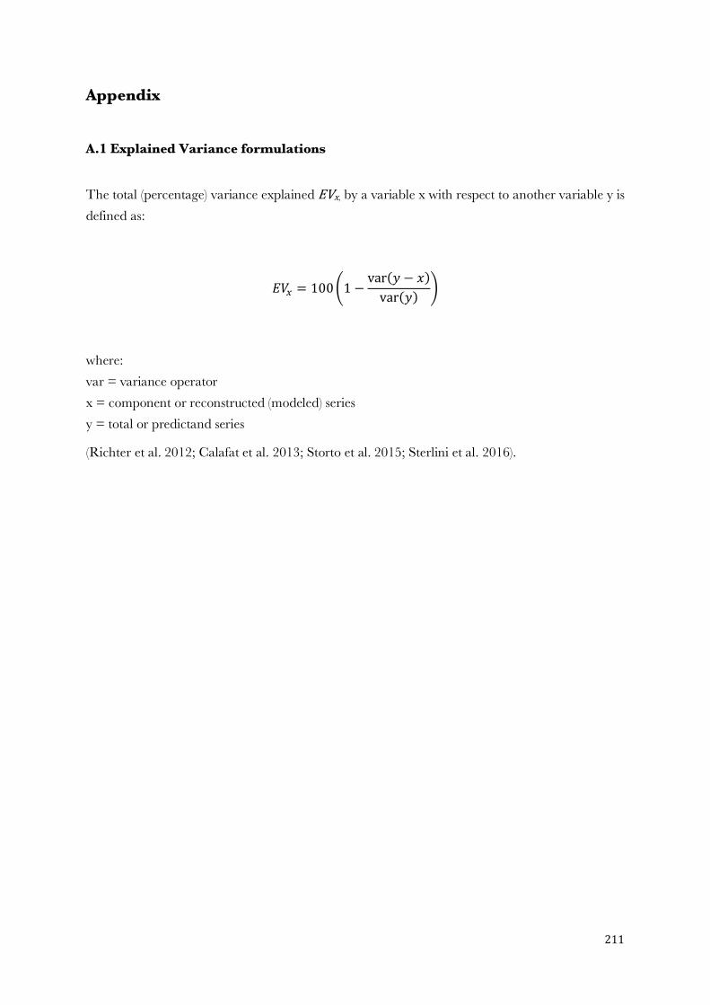
211

Appendix

A.1 Explained Variance formulations

The total (percentage) variance explainedEVx, by a variable x with respect to another variable y is defined as:

'() = 100-1 − var(2 − 3)var(2) 5

where: var = variance operator x = component or reconstructed (modeled) series y = total or predictand series

(Richter et al. 2012; Calafat et al. 2013; Storto et al. 2015; Sterlini et al. 2016).

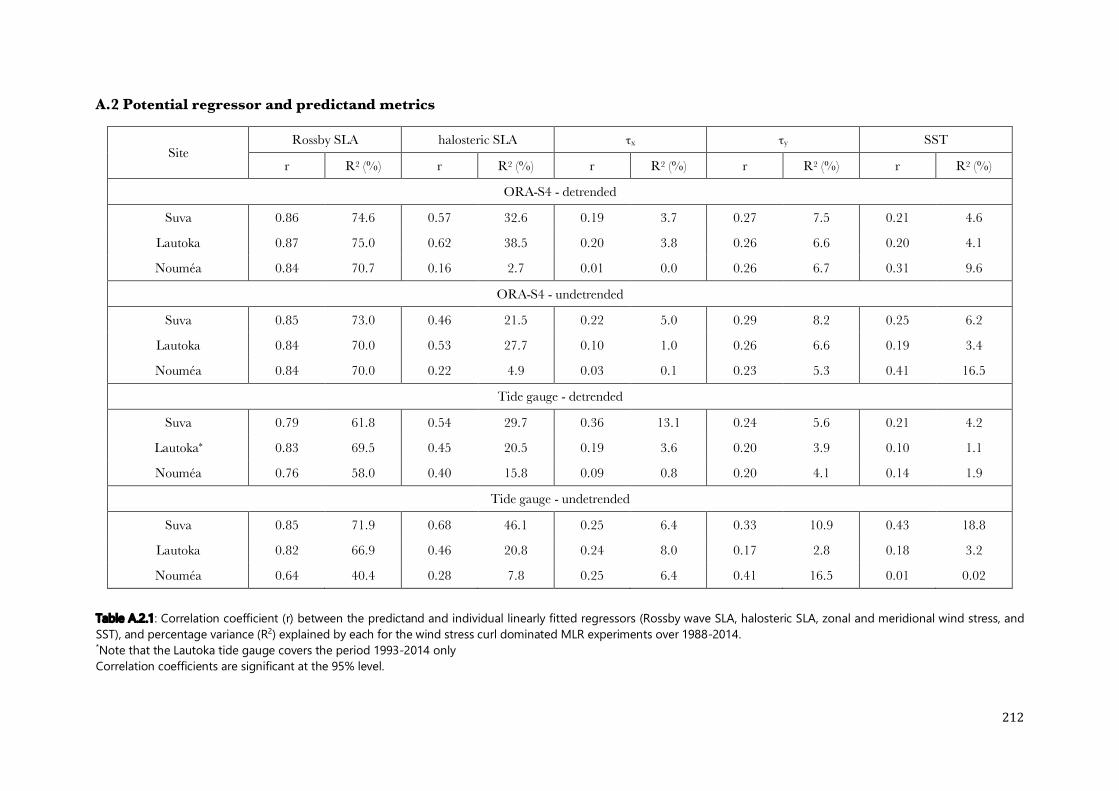
212

A.2 Potential regressor and predictand metrics

Site Rossby SLA halosteric SLA τx τy SST

r R2 (%) r R2 (%) r R2 (%) r R2 (%) r R2 (%)

ORA-S4 - detrended

Suva 0.86 74.6 0.57 32.6 0.19 3.7 0.27 7.5 0.21 4.6

Lautoka 0.87 75.0 0.62 38.5 0.20 3.8 0.26 6.6 0.20 4.1

Nouméa 0.84 70.7 0.16 2.7 0.01 0.0 0.26 6.7 0.31 9.6


Suva 0.85 73.0 0.46 21.5 0.22 5.0 0.29 8.2 0.25 6.2

Lautoka 0.84 70.0 0.53 27.7 0.10 1.0 0.26 6.6 0.19 3.4

Nouméa 0.84 70.0 0.22 4.9 0.03 0.1 0.23 5.3 0.41 16.5


Suva 0.79 61.8 0.54 29.7 0.36 13.1 0.24 5.6 0.21 4.2

Lautoka* 0.83 69.5 0.45 20.5 0.19 3.6 0.20 3.9 0.10 1.1

Nouméa 0.76 58.0 0.40 15.8 0.09 0.8 0.20 4.1 0.14 1.9


Suva 0.85 71.9 0.68 46.1 0.25 6.4 0.33 10.9 0.43 18.8

Lautoka 0.82 66.9 0.46 20.8 0.24 8.0 0.17 2.8 0.18 3.2

Nouméa 0.64 40.4 0.28 7.8 0.25 6.4 0.41 16.5 0.01 0.02

Table A.2.1: Correlation coefficient (r) between the predictand and individual linearly fitted regressors (Rossby wave SLA, halosteric SLA, zonal and meridional wind stress, and SST), and percentage variance (R2) explained by each for the wind stress curl dominated MLR experiments over 1988-2014. *Note that the Lautoka tide gauge covers the period 1993-2014 only Correlation coefficients are significant at the 95% level.

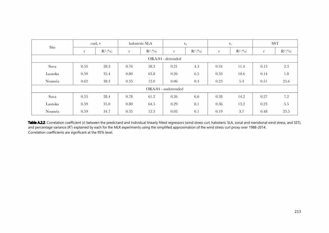
213

Table A.2.2: Correlation coefficient (r) between the predictand and individual linearly fitted regressors (wind stress curl, halosteric SLA, zonal and meridional wind stress, and SST), and percentage variance (R2) explained by each for the MLR experiments using the simplified approximation of the wind stress curl proxy over 1988-2014. Correlation coefficients are significant at the 95% level.

Site curlz τ halosteric SLA τx τy SST

r R2 (%) r R2 (%) r R2 (%) r R2 (%) r R2 (%)

ORA-S4 - detrended

Suva 0.53 28.3 0.76 58.3 0.21 4.3 0.34 11.4 0.15 2.3

Lautoka 0.59 35.4 0.80 63.8 0.26 6.5 0.33 10.6 0.14 1.8

Nouméa 0.62 38.3 0.35 12.0 0.06 0.3 0.23 5.4 0.51 25.6


Suva 0.53 28.4 0.78 61.2 0.26 6.6 0.38 14.2 0.27 7.2

Lautoka 0.59 35.0 0.80 64.5 0.29 8.1 0.36 13.2 0.23 5.5

Nouméa 0.59 34.7 0.35 12.3 0.03 0.1 0.19 3.7 0.48 23.5

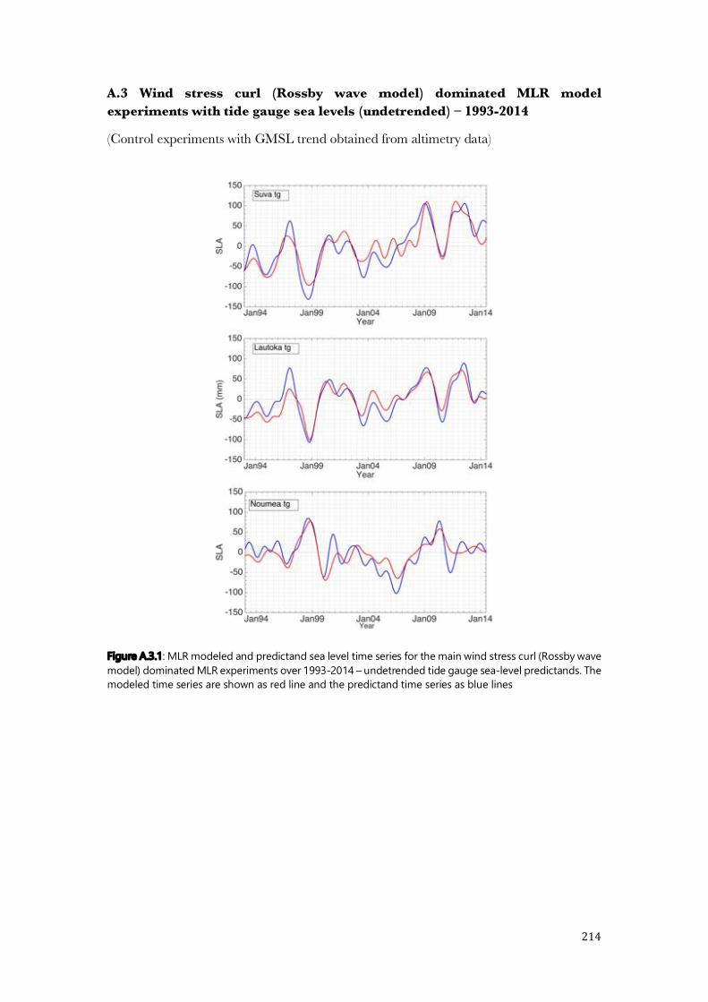
214

A.3 Wind stress curl (Rossby wave model) dominated MLR model experiments with tide gauge sea levels (undetrended) – 1993-2014

(Control experiments with GMSL trend obtained from altimetry data)

Figure A.3.1: MLR modeled and predictand sea level time series for the main wind stress curl (Rossby wave

model) dominated MLR experiments over 1993-2014 – undetrended tide gauge sea-level predictands. The

modeled time series are shown as red line and the predictand time series as blue lines

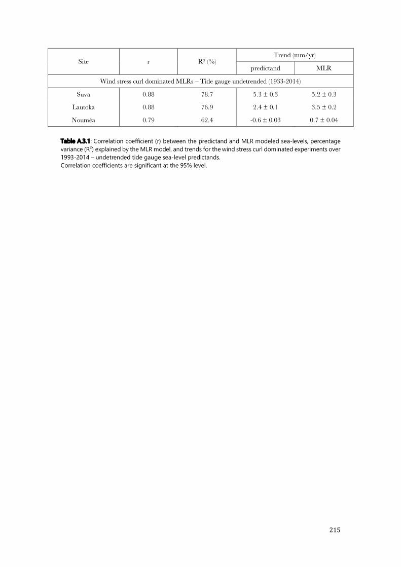
215

Site r R2 (%) Trend (mm/yr)

predictand MLR


Suva 0.88 78.7 5.3 ± 0.3 5.2 ± 0.3

Lautoka 0.88 76.9 2.4 ± 0.1 3.5 ± 0.2

Nouméa 0.79 62.4 -0.6 ± 0.03 0.7 ± 0.04

Table A.3.1: Correlation coefficient (r) between the predictand and MLR modeled sea-levels, percentage variance (R2) explained by the MLR model, and trends for the wind stress curl dominated experiments over 1993-2014 – undetrended tide gauge sea-level predictands. Correlation coefficients are significant at the 95% level.

216

A.4 Stationarity test MLR equations


Coefficient Rossby

SLA halo τx τy SST

ORA-S4 – detrended – 1st half (Aug 1988 – Jul 2001)

Suva 0.55 0.73 0.48 -997.95 -1.64e+3 x

Lautoka 1.22 0.69 0.57 -785.17 x 14.17

Nouméa 1.00 0.72 0.43 -309.15 x 15.46

ORA-S4 – detrended – 2nd half (Aug 2001 – Jul 2014)

Suva -1.34 0.74 1.02 -1.51e+3 -1.77e+3 x

Lautoka -0.82 0.73 0.45 -1.53e+3 x 18.80

Nouméa -0.57 0.85 0.16 -2.65e+3 x 3.17

ORA-S4 – undetrended – 1st half (Aug 1988 – Jul 2001)

Suva 3.14 0.71 0.59 -934.76 -1.80e+3 -13.51

Lautoka 4.34 0.61 0.76 -907.58 x x

Nouméa 6.10 0.70 0.53 x 96.70 21.93

ORA-S4 – undetrended – 2nd half (Aug 2001 – Jul 2014)

Suva -4.62 0.73 0.92 -1.82e+3 -1.81e+3 10.09

Lautoka -3.34 0.58 0.60 -1.38e+3 x x

Nouméa -0.24 0.85 0.10 x -2.67e+3 10.09

Tide gauge – detrended – 1st half (Aug 1988 – Jul 2001)

Suva 4.13 0.57 -0.97 1.28e+3 x 16.47

Lautoka* 2.58 0.90 0.26 2.81 -791.76 x

Nouméa 2.56 0.70 0.86 x x 22.05

Tide gauge – detrended – 2nd half (Aug 2001 – Jul 2014)

Suva -3.55 0.71 -0.40 -805.70 x 32.72

Lautoka* -1.09 0.80 0.52 -1.33e+3 -2.05e+3 x

Nouméa -2.67 0.77 1.05 x x 16.05

Tide gauge – undetrended – 1st half (Aug 1988 – Jul 2001)

Suva 7.15 0.65 -0.81 1.13e+3 561.77 30.51

Lautoka* 9.89 0.68 0.75 -658.96 -661.18 x

Nouméa 8.77 0.71 0.79 -2.38e+3 x -33.23

Tide gauge – undetrended – 2nd half (Aug 2001 – Jul 2014)

Suva -5.06 0.69 -0.53 -839.5 -1.30e+3 18.60

Lautoka* -13.37 0.85 0.83 -1.02e+3 -1.67e+3 x

Nouméa -19.23 0.78 0.79 x -2.35e+3 1.25

Table A.4.1: Stationarity test MLR model equations for the main wind stress curl (Rossby wave model)

dominated experiments over 1988-2014. x marks regressors not included in the MLR model. *Note that for the Lautoka tide gauge (1993-2014), 1

st half covers Jan 1993 – Oct 2003 and 2

nd half covers

Nov 2003 – Jul 2014.

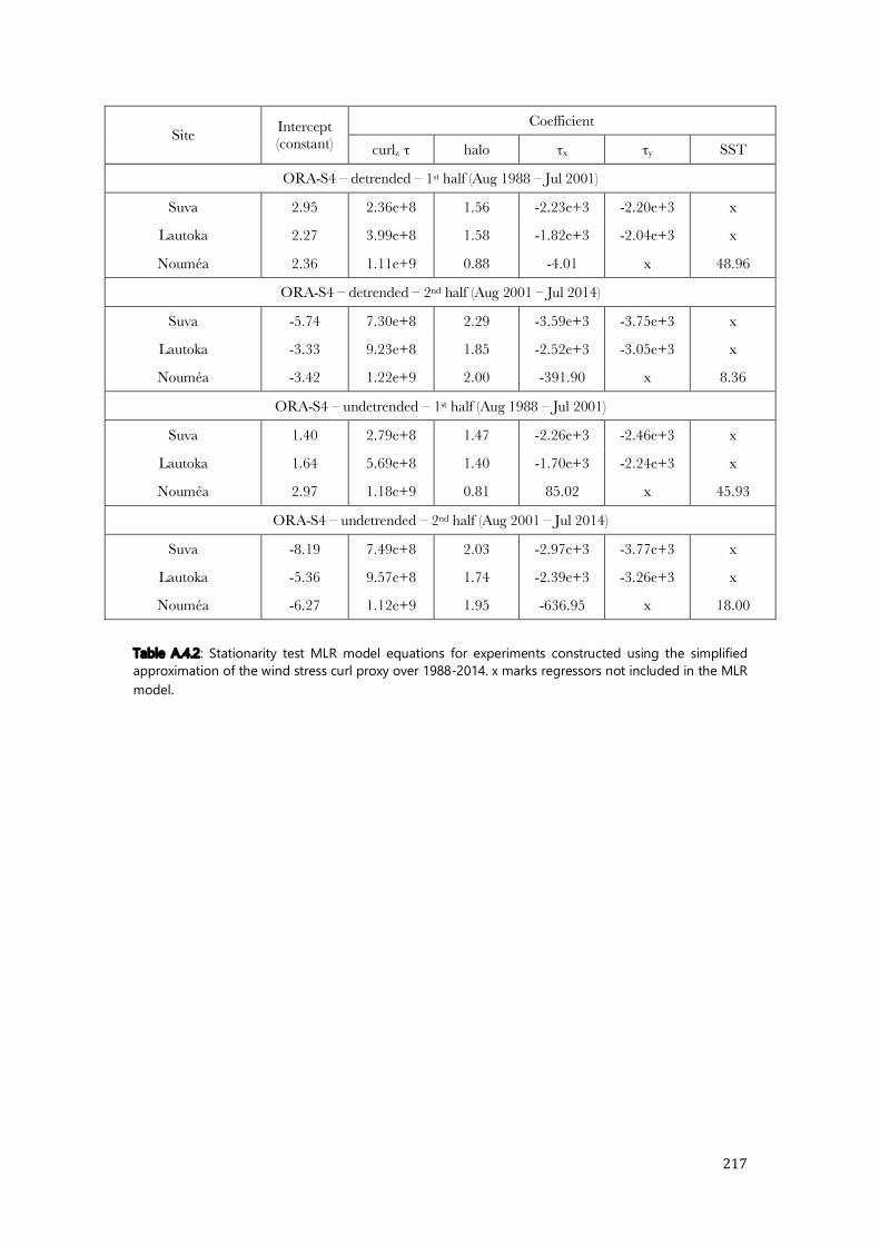
217


Coefficient

curlz τ halo τx τy SST

ORA-S4 – detrended – 1st half (Aug 1988 – Jul 2001)

Suva 2.95 2.36e+8 1.56 -2.23e+3 -2.20e+3 x

Lautoka 2.27 3.99e+8 1.58 -1.82e+3 -2.04e+3 x

Nouméa 2.36 1.11e+9 0.88 -4.01 x 48.96

ORA-S4 – detrended – 2nd half (Aug 2001 – Jul 2014)

Suva -5.74 7.30e+8 2.29 -3.59e+3 -3.75e+3 x

Lautoka -3.33 9.23e+8 1.85 -2.52e+3 -3.05e+3 x

Nouméa -3.42 1.22e+9 2.00 -391.90 x 8.36

ORA-S4 – undetrended – 1st half (Aug 1988 – Jul 2001)

Suva 1.40 2.79e+8 1.47 -2.26e+3 -2.46e+3 x

Lautoka 1.64 5.69e+8 1.40 -1.70e+3 -2.24e+3 x

Nouméa 2.97 1.18e+9 0.81 85.02 x 45.93

ORA-S4 – undetrended – 2nd half (Aug 2001 – Jul 2014)

Suva -8.19 7.49e+8 2.03 -2.97e+3 -3.77e+3 x

Lautoka -5.36 9.57e+8 1.74 -2.39e+3 -3.26e+3 x

Nouméa -6.27 1.12e+9 1.95 -636.95 x 18.00

Table A.4.2: Stationarity test MLR model equations for experiments constructed using the simplified

approximation of the wind stress curl proxy over 1988-2014. x marks regressors not included in the MLR

model.

219

Annex 1

Peer-reviewed article

221

RESEARCH ARTICLE10.1002/2017JC013053

Reconstruction of Local Sea Levels at South West PacificIslands—A Multiple Linear Regression Approach (1988–2014)V. Kumar1,4 , A. Melet2, B. Meyssignac1 , A. Ganachaud1 , W. S. Kessler3, A. Singh4 , andJ. Aucan5

1LEGOS, Universit!e de Toulouse, CNES, CNRS, IRD, UPS, Toulouse, France, 2Mercator Ocean, Ramonville-Saint-Agne,France, 3NOAA/Pacific Marine Environmental Laboratory, Seattle, WA, USA, 4PaCE-SD, University of the South Pacific, Suva,Fiji, 5LEGOS, Universit!e de Toulouse, CNES, CNRS, IRD, UPS, Noum!ea, New Caledonia, France

Abstract Rising sea levels are a critical concern in small island nations. The problem is especially seriousin the western south Pacific, where the total sea level rise over the last 60 years has been up to 3 times theglobal average. In this study, we aim at reconstructing sea levels at selected sites in the region (Suva,Lautoka—Fiji, and Noum!ea—New Caledonia) as a multilinear regression (MLR) of atmospheric and oceanicvariables. We focus on sea level variability at interannual-to-interdecadal time scales, and trend over the1988–2014 period. Local sea levels are first expressed as a sum of steric and mass changes. Then a dynami-cal approach is used based on wind stress curl as a proxy for the thermosteric component, as wind stresscurl anomalies can modulate the thermocline depth and resultant sea levels via Rossby wave propagation.Statistically significant predictors among wind stress curl, halosteric sea level, zonal/meridional wind stresscomponents, and sea surface temperature are used to construct a MLR model simulating local sea levels.Although we are focusing on the local scale, the global mean sea level needs to be adjusted for. Our recon-structions provide insights on key drivers of sea level variability at the selected sites, showing that whilelocal dynamics and the global signal modulate sea level to a given extent, most of the variance is driven byregional factors. On average, the MLR model is able to reproduce 82% of the variance in island sea level,and could be used to derive local sea level projections via downscaling of climate models.

1. Introduction

Sea level rise is one of the most important threats related to global warming and associated climate changein the Pacific islands. Unlike other long-term climate-related threats, rising sea levels are no longer a distanthazard, but present reality in many coastal communities (Hallegatte et al., 2013; Neumann et al., 2015;Wong et al., 2014). Most Pacific islands have a high population density and infrastructure concentratedalong the coastal zones (Nurse et al., 2014; Webb & Kench, 2010; Wong et al., 2014). These factors, combinedwith others, such as geographical isolation, limited financial resources, and technical expertise, make theislands among the most vulnerable in the world to the growing threats of sea level rise (Barnett & Campbell,2010; Garschagen et al., 2016; Mimura, 1999; Wong et al., 2014).

The Pacific islands are characterized by high-rise volcanic formations and low-lying reef atolls. While the lat-ter are more endangered, and face the likelihood of inundation by the end of the 21st century, even themountainous islands have had communities forced to relocate due to saltwater intrusion, perigean springtide events, and flash floods during extreme events (Albert et al., 2016; McNamara & Jacot Des Combes,2015; Nurse et al., 2014; OCHA—United Nations, 2014). As warming continues, sea level will continue to rise(Church et al., 2013), further exacerbating coastal impacts. Thus, there is a compelling need for informationon regional sea level variability and its key drivers to help plan proper adaptation measures and buildcapacity for climate resilience.

According to analysis of tide gauge records, the global mean sea level (GMSL) rose at a rate of !1.5 60.4 mm/yr between 1901 and 2010, accounting for a total rise of around 0.17 m during that period (Church& White, 2011; Hay et al., 2015; Jevrejeva et al., 2008; Ray & Douglas, 2011). Satellite altimetry reports a fasterglobal mean rate of 3.1 6 0.5 mm/yr over 1993–2016. Yet, sea level rise is far from being spatially uniform.During the satellite altimetry era, for example, sea levels in the western tropical Pacific rose at rates up to

Key Points:" Local sea level variability on

interannual-to-interdecadal timescales in the area is governed mainlyby the regional wind field" These regional winds could be

simulated by climate models, servingas a link between local scaleinformation and low resolutionmodels" Mass contribution from melt of

glaciers and ice sheets is muchsmaller relative to the dominantsteric component

Supporting Information:" Supporting Information S1

Correspondence to:A. Ganachaud,[email protected]

Citation:Kumar, V., Melet, A., Meyssignac, B.,Ganachaud, A., Kessler, W. S., Singh, A.,& Aucan, J. (2018). Reconstruction oflocal sea levels at South West PacificIslands—A Multiple linear regressionapproach (1988–2014). Journal ofGeophysical Research: Oceans, 123,1502–1518. https://doi.org/10.1002/2017JC013053

Received 3 MAY 2017Accepted 30 JAN 2018Accepted article online 5 FEB 2018Published online 27 FEB 2018

VC 2018. American Geophysical Union.All Rights Reserved.

KUMAR ET AL. 1502

Journal of Geophysical Research: Oceans

PUBLICATIONS

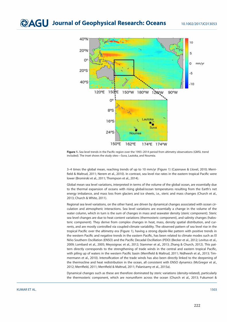
222

3–4 times the global mean, reaching trends of up to 10 mm/yr (Figure 1) (Cazenave & Llovel, 2010; Merri-field & Maltrud, 2011; Nerem et al., 2010). In contrast, sea level rise rates in the eastern tropical Pacific werelower (Bromirski et al., 2011; Thompson et al., 2014).

Global mean sea level variations, interpreted in terms of the volume of the global ocean, are essentially dueto the thermal expansion of oceans with rising global/ocean temperatures resulting from the Earth’s netenergy imbalance, and mass loss from glaciers and ice sheets, i.e., steric and mass changes (Church et al.,2013; Church & White, 2011).

Regional sea level variations, on the other hand, are driven by dynamical changes associated with ocean cir-culation and atmospheric interactions. Sea level variations are essentially a change in the volume of thewater column, which in turn is the sum of changes in mass and seawater density (steric component). Stericsea level changes are due to heat content variations (thermosteric component), and salinity changes (halos-teric component). They derive from complex changes in heat, mass, density spatial distribution, and cur-rents, and are mostly controlled via coupled-climate variability. The observed pattern of sea level rise in thetropical Pacific over the altimetry era (Figure 1), having a strong dipole-like pattern with positive trends inthe western Pacific and negative trends in the eastern Pacific, has been related to climate modes such as ElNi~no Southern Oscillation (ENSO) and the Pacific Decadal Oscillation (PDO) (Becker et al., 2012; Levitus et al.,2009; Lombard et al., 2005; Meyssignac et al., 2012; Stammer et al., 2013; Zhang & Church, 2012). This pat-tern directly corresponds to the strengthening of trade winds in the central and eastern tropical Pacific,with piling up of waters in the western Pacific basin (Merrifield & Maltrud, 2011; Nidheesh et al., 2013; Tim-mermann et al., 2010). Intensification of the trade winds has also been directly linked to the deepening ofthe thermocline and heat redistribution in the ocean, all consistent with ENSO dynamics (McGregor et al.,2012; Merrifield, 2011; Merrifield & Maltrud, 2011; Palanisamy et al., 2015a).

Dynamical changes such as these are therefore dominated by steric variations (density-related), particularlythe thermosteric component, which are nonuniform across the ocean (Church et al., 2013; Fukumori &

Figure 1. Sea level trends in the Pacific region over the 1993–2014 period from altimetry observations (GMSL trendincluded). The inset shows the study sites—Suva, Lautoka, and Noum!ea.

Journal of Geophysical Research: Oceans 10.1002/2017JC013053

KUMAR ET AL. 1503

223

Wang, 2013; Gregory & Lowe, 2000; Levitus et al., 2005, 2012; Lombard et al., 2005, 2009; Meyssignac &Cazenave, 2012; Stammer et al., 2013).

Thermosteric sea level trends in the tropical Pacific have been shown to be driven by surface wind stressand related changes in circulation patterns in ocean numerical models (Carton et al., 2005; K€ohl et al., 2007;McGregor et al., 2012; Nidheesh et al., 2013; Timmermann et al., 2010). Wind stress curl anomalies can con-trol the thermocline depth and the resultant sea levels in the tropical Pacific by modulating the near-surface Ekman transport, Ekman pumping, and consequent oceanic Rossby waves. As such, wind stressplays a critical role in determining and/or reproducing regional sea level trends.

Additionally, regional sea level change also includes other processes, such as the inverted barometer effect(atmospheric loading) (Wunsch & Stammer, 1997), and the glacial isostatic adjustment (GIA) (Peltier, 2004).However, their effects relative to thermosteric and halosteric changes, especially in the tropics, are small,and can be described as a larger scale signature in terms of sea level.

In coastal zones, sea level change is a composite of the global mean sea level, regional processes, andlocal modulations (Melet et al., 2016a; Milne et al., 2009; Stammer et al., 2013). At local scales, sea levelvariations can be induced by atmospheric surges due to wind and pressure effects, wave-induced setupand run up, and tides. Relative sea level at the coast can further be influenced by site-specific geographicfeatures associated with vertical land motion. This can be in the form of land subsidence, or even upliftdue to natural causes such as earthquakes, volcanic activity, other tectonic processes, and sedimentation,or due to anthropogenic activities such as groundwater pumping (Ballu et al., 2011; Stammer et al., 2013;Wong et al., 2014).

Based on this knowledge of processes determining local sea level changes, we aim to simulate sea level atselected sites in the southwest Pacific. Our objective is to express sea level as a multiple linear regression(MLR) of statistically determined variables, representing remote and local drivers. For this study, we focuson interannual-to-interdecadal time scale sea level variability and trend. The MLR we develop providesinsights and a better understanding of the different drivers of sea level variations in the region. With a sta-tistical model such as this, projections from coarse resolution climate models can be refined on the localscale for future applications (Church et al., 2013).

Our study sites are (1) Suva and (2) Lautoka in Fiji, and (3) Noum"ea in New Caledonia (Figure 1). These siteshave been selected based on their vulnerability to sea level rise (Garschagen et al., 2016; Wong et al., 2014).The selection can be perceived as a preliminary step to research that can be applied at more extensivescales, covering more sites in future projections of sea level trends in the region. Having such informationavailable on local scales in vulnerable regions, more effective adaptation and risk minimization measurescould be developed.

2. Data Sets

2.1. Tide Gauge RecordsMonthly mean Revised Local Reference (RLR) tide gauge records for Suva and Lautoka were retrieved fromthe Permanent Service for Mean Sea level (PSMSL, http://www.psmsl.org) (Holgate et al., 2013). For Noum"ea,a merged sea level series from sites Chaleix and Numbo was used (Aucan et al., 2017).

Details on the tide gauge records used are shown in Table 1.

Table 1Tide Gauge Station Data for Suva, Lautoka, and Noumea, With Longitude/Latitude Coordinates, Data Duration, andPercentage of Missing Data

Site Grid locationPSMSL

station IDa Duration% of gap (max. length

in consecutive months)

Suva 178.428E, 18.148S 1327 Oct 1972 to Dec 2014 6 (6)Lautoka 177.448E, 17.608S 1805 Nov 1992 to Dec 2014 0.4 (1)Noum"ea 166.438E, 22.308S Feb 1967 to Dec 2014 2 (11)

aFor Suva and Lautoka only.


KUMAR ET AL. 1504

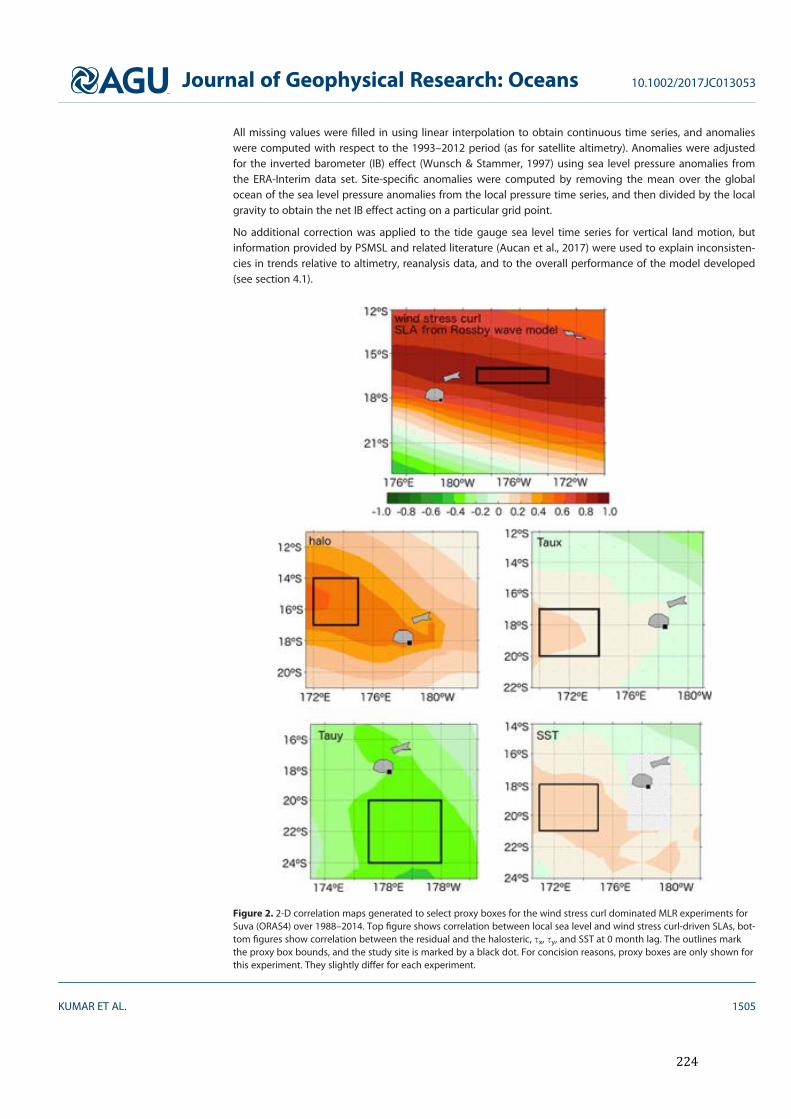
224

All missing values were filled in using linear interpolation to obtain continuous time series, and anomalieswere computed with respect to the 1993–2012 period (as for satellite altimetry). Anomalies were adjustedfor the inverted barometer (IB) effect (Wunsch & Stammer, 1997) using sea level pressure anomalies fromthe ERA-Interim data set. Site-specific anomalies were computed by removing the mean over the globalocean of the sea level pressure anomalies from the local pressure time series, and then divided by the localgravity to obtain the net IB effect acting on a particular grid point.

No additional correction was applied to the tide gauge sea level time series for vertical land motion, butinformation provided by PSMSL and related literature (Aucan et al., 2017) were used to explain inconsisten-cies in trends relative to altimetry, reanalysis data, and to the overall performance of the model developed(see section 4.1).

Figure 2. 2-D correlation maps generated to select proxy boxes for the wind stress curl dominated MLR experiments forSuva (ORAS4) over 1988–2014. Top figure shows correlation between local sea level and wind stress curl-driven SLAs, bot-tom figures show correlation between the residual and the halosteric, sx, sy, and SST at 0 month lag. The outlines markthe proxy box bounds, and the study site is marked by a black dot. For concision reasons, proxy boxes are only shown forthis experiment. They slightly differ for each experiment.


KUMAR ET AL. 1505

225

2.2. Altimetric Sea LevelTo compare the tide gauge records with altimetry data, 2-D gridded sea surface height delayed timeanomalies produced by the Ssalto/DUACS system and distributed by the Copernicus Marine and Environ-ment Monitoring Service (CMEMS, product 008–027, Retrieved from http://marine.copernicus.eu/,accessed 20 January 2016) were used over the period 1993–2014. The data set is provided at weekly inter-vals on a 1=48 regular grid as anomalies computed with reference to the 1993–2012 period. Sea levelanomalies for the study sites were extracted from the global data set using distance weighted remappingfor the corresponding longitude/latitude coordinates in the tide gauge records.

2.3. ERA-Interim Data (Wind, SST, SLP Data)ERA-Interim is the European Center for Medium-Range Weather Forecast’s (ECMWF’s) global atmosphericreanalysis product (Dee et al., 2011; retrieved in 2016). It extends back in time until 1988, and is continu-ously updated in near real time.

Zonal and meridional surface wind stress fields (sx, sy), mean sea levelpressure (SLP), and sea surface temperature (SST) data sets wereextracted from ERA-Interim for the duration of the data set, asmonthly means and at a resolution of 18 3 18.

2.4. ECMWF Ocean Reanalysis System 4—ORAS4Local sea levels were taken from a reanalysis product, in addition totide gauge record observations. The main reason for doing this is thattide gauge records typically have gaps, and may show biased trendsdue to vertical land motion (as for the Suva tide gauge) (PSMSL,2016).

We use ORAS4, which is among reanalysis products that have goodcomparison with the tide gauge sea levels (Balmaseda et al., 2015)used in this study (Figure 3), and have steric sea levels lying within thespread of a reanalysis ensemble (Storto et al., 2015), making it a repre-sentative reanalysis product. ORAS4 spans a period from 1958 to pre-sent. From 1989 to 2010, the surface fluxes in the reanalysis are fromERA-Interim (Balmaseda et al., 2013). Thus, there is consistencybetween the wind, SST, and SLP data we are using for this study overmost of our period of interest (1988–2014). ORAS4 uses a Boussinesqapproximation, where the ocean model preserves volume. The stericcomponent of the global mean sea level is thus not represented bythe model, but estimated by vertically integrating the density field ofthe ocean analysis and added to the sea level output. ORAS4 does notmodel land ice melt and thus does not represent directly the oceanmass increase due to land ice loss. The ocean mass increase due toland ice loss is estimated at each time step n from altimetry observa-tions corrected for the thermosteric sea level from ORAS4 of time stepn-1. This land ice loss estimate is then added to the water flux fromthe atmosphere in the form of a uniform water flux over the ocean. Inthe end in the ORAS4 sea level output both components of the sealevel rise are present: the thermosteric and the ocean mass. For thisreason, the ORAS4 GMSL includes all terms and is consistent with theGMSL from the altimeter data (Balmaseda et al., 2013).

Ocean temperature, salinity, and sea surface height fields wereextracted from ORAS4 as monthly means, and at 18 3 18 resolutionfor the period 1988–2014. Thermosteric, halosteric, and total steric sealevels were computed for depths of 0–700 m using the Gibbs Seawa-ter Toolbox (McDougall & Barker, 2011). Sea surface heights at the

Figure 3. Sea level time series at (top) Suva, (middle) Lautoka, and (bottom)Noum!ea over the 1988–2014 period. Blue lines represent tide gauges, greenlines represent ORAS4, and magenta shows altimetry time series.


KUMAR ET AL. 1506

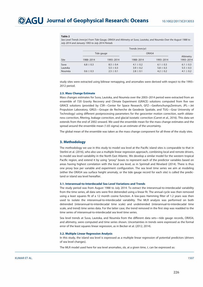
226

study sites were extracted using bilinear remapping, and anomalies were derived with respect to the 1993–2012 period.

2.5. Mass Change EstimateMass changes estimates for Suva, Lautoka, and Noum!ea over the 2003–2014 period were extracted from anensemble of 720 Gravity Recovery and Climate Experiment (GRACE) solutions computed from five rawGRACE solutions (provided by CSR—Center for Space Research, GFZ—GeoforschungsZentrum, JPL—JetPropulsion Laboratory, GRGS—Groupe de Recherche de Geodesie Spatiale, and TUG—Graz University ofTechnology) using different postprocessing parameters for the geocenter motion correction, earth oblate-ness correction, filtering, leakage correction, and glacial isostatic correction (Carret et al., 2016). This data setextends from the end of 2002 onward. We used the ensemble mean for the mass change estimates and thespread around the ensemble mean (1.65 sigma) as an estimate of the uncertainty.

The global mean of the ensemble was taken as the mass change component for all three of the study sites.

3. Methodology

The methodology we use in this study to model sea level at the Pacific island sites is comparable to that inSterlini et al. (2016), who also use a multiple linear regression approach, combining local and remote drivers,to model sea level variability in the North East Atlantic. We develop a similar model for the western tropicalPacific region, and extend it by using ‘‘proxy’’ boxes to represent each of the predictor variables based onareas having highest correlation with the local sea level, as in Sprintall and R!evelard (2014). There is thusone proxy box per variable and experiment configuration. The sea level time series we aim at modeling(either the ORAS4 sea surface height anomaly, or the tide gauge record for each site) is called the predic-tand or island sea level hereafter.

3.1. Interannual-to-Interdecadal Sea Level Variations and TrendsThe study period was from August 1988 to July 2014. To extract the interannual-to-interdecadal variabilityfrom the time series, all data sets were first detrended using a linear fit. The annual cycle was then removedusing a least squares fit of a 12 month cosine function. A low-pass Hamming filter of 1.2 years was thenused to isolate the interannual-to-interdecadal variability. The MLR analysis was performed on bothdetrended (interannual-to-interdecadal time scale) and undetrended (interannual-to-interdecadal timescale, and trend) time series data. For the latter case, the trend removed in the first step was readded to thetime series of interannual-to-interdecadal sea level time series.

Sea level trends at Suva, Lautoka, and Noum!ea from the different data sets—tide gauge records, ORAS4,and altimetry, were computed and time series shown. Uncertainties in trends were expressed as the formalerror of the least squares linear regression, as in Becker et al. (2012, 2014).

3.2. Multiple Linear Regression AnalysisIn this study, the island sea level is expressed as a multiple linear regression of potential predictors (driversof sea level changes).

The MLR model used here for sea level anomalies, sla, at a given time, t, can be expressed as:

Table 2Sea Level Trends (mm/yr) From Tide Gauge, ORAS4 and Altimetry at Suva, Lautoka, and Noum!ea Over the August 1988 toJuly 2014 and January 1993 to July 2014 Periods

Site

Trends (mm/yr)

Tide gauge ORAS4Altimetry

1988–2014 1993–2014 1988–2014 1993–2014 1993–2014

Suva 6.8 6 0.3 8.5 6 0.4 4.1 6 0.2 6.1 6 0.3 6.1 6 0.3Lautoka 5.5 6 0.3 3.9 6 0.2 5.8 6 0.3 5.5 6 0.3Noum!ea 0.6 6 0.3 2.5 6 0.1 2.8 6 0.1 4.2 6 0.2 4.1 6 0.2


KUMAR ET AL. 1507

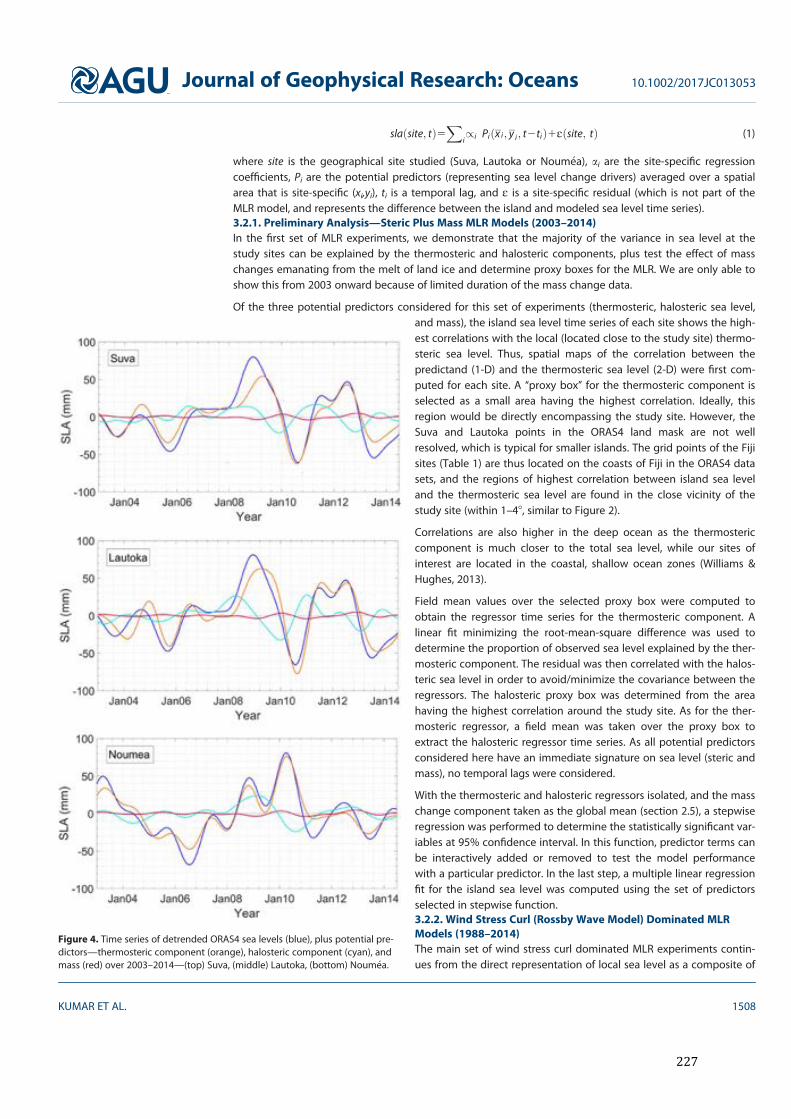
227

sla site; tð Þ5X

i/i Pi x i ; y i ; t2tið Þ1E site; tð Þ (1)

where site is the geographical site studied (Suva, Lautoka or Noum!ea), ai are the site-specific regressioncoefficients, Pi are the potential predictors (representing sea level change drivers) averaged over a spatialarea that is site-specific (xi,yi), ti is a temporal lag, and E is a site-specific residual (which is not part of theMLR model, and represents the difference between the island and modeled sea level time series).3.2.1. Preliminary Analysis—Steric Plus Mass MLR Models (2003–2014)In the first set of MLR experiments, we demonstrate that the majority of the variance in sea level at thestudy sites can be explained by the thermosteric and halosteric components, plus test the effect of masschanges emanating from the melt of land ice and determine proxy boxes for the MLR. We are only able toshow this from 2003 onward because of limited duration of the mass change data.

Of the three potential predictors considered for this set of experiments (thermosteric, halosteric sea level,and mass), the island sea level time series of each site shows the high-est correlations with the local (located close to the study site) thermo-steric sea level. Thus, spatial maps of the correlation between thepredictand (1-D) and the thermosteric sea level (2-D) were first com-puted for each site. A ‘‘proxy box’’ for the thermosteric component isselected as a small area having the highest correlation. Ideally, thisregion would be directly encompassing the study site. However, theSuva and Lautoka points in the ORAS4 land mask are not wellresolved, which is typical for smaller islands. The grid points of the Fijisites (Table 1) are thus located on the coasts of Fiji in the ORAS4 datasets, and the regions of highest correlation between island sea leveland the thermosteric sea level are found in the close vicinity of thestudy site (within 1–48, similar to Figure 2).

Correlations are also higher in the deep ocean as the thermostericcomponent is much closer to the total sea level, while our sites ofinterest are located in the coastal, shallow ocean zones (Williams &Hughes, 2013).

Field mean values over the selected proxy box were computed toobtain the regressor time series for the thermosteric component. Alinear fit minimizing the root-mean-square difference was used todetermine the proportion of observed sea level explained by the ther-mosteric component. The residual was then correlated with the halos-teric sea level in order to avoid/minimize the covariance between theregressors. The halosteric proxy box was determined from the areahaving the highest correlation around the study site. As for the ther-mosteric regressor, a field mean was taken over the proxy box toextract the halosteric regressor time series. As all potential predictorsconsidered here have an immediate signature on sea level (steric andmass), no temporal lags were considered.

With the thermosteric and halosteric regressors isolated, and the masschange component taken as the global mean (section 2.5), a stepwiseregression was performed to determine the statistically significant var-iables at 95% confidence interval. In this function, predictor terms canbe interactively added or removed to test the model performancewith a particular predictor. In the last step, a multiple linear regressionfit for the island sea level was computed using the set of predictorsselected in stepwise function.3.2.2. Wind Stress Curl (Rossby Wave Model) Dominated MLRModels (1988–2014)The main set of wind stress curl dominated MLR experiments contin-ues from the direct representation of local sea level as a composite of

Figure 4. Time series of detrended ORAS4 sea levels (blue), plus potential pre-dictors—thermosteric component (orange), halosteric component (cyan), andmass (red) over 2003–2014—(top) Suva, (middle) Lautoka, (bottom) Noum!ea.


KUMAR ET AL. 1508

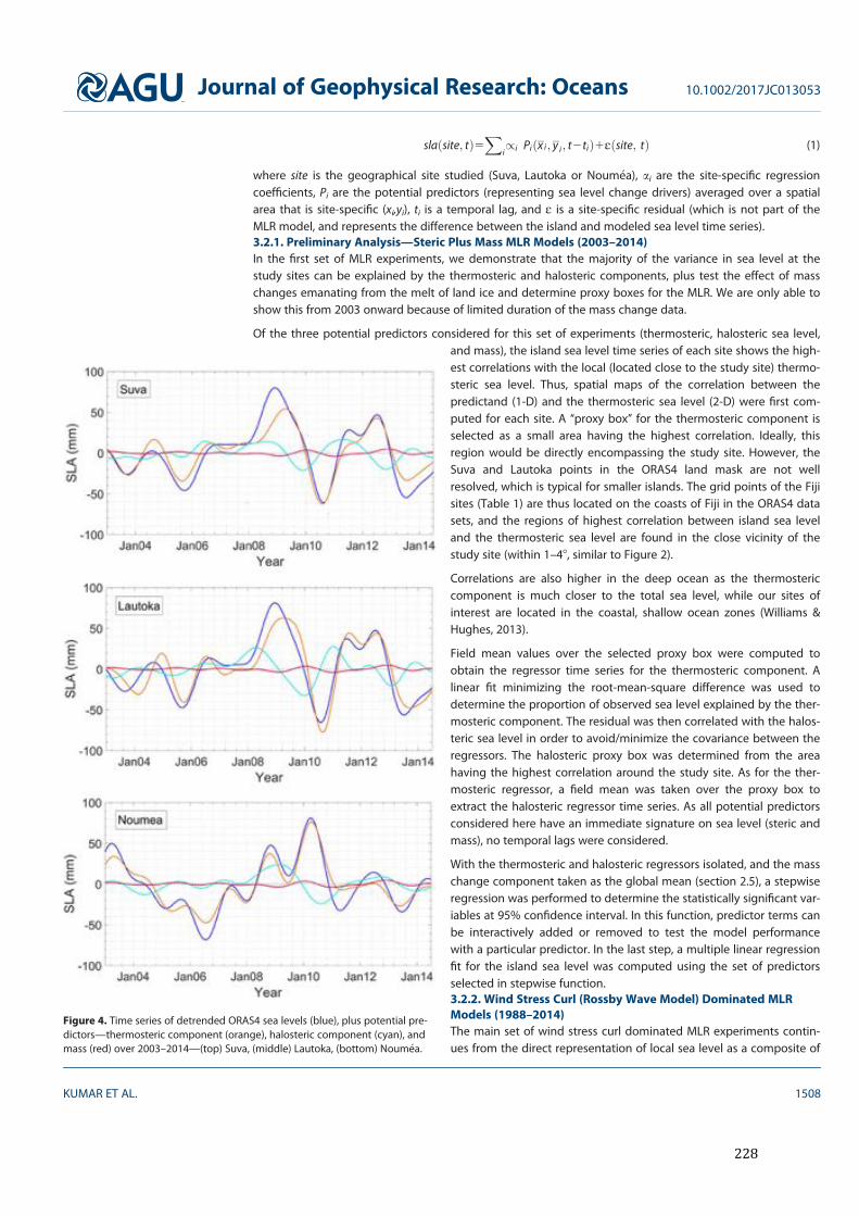
228

sla site; tð Þ5X

i/i Pi x i ; y i ; t2tið Þ1E site; tð Þ (1)

where site is the geographical site studied (Suva, Lautoka or Noum!ea), ai are the site-specific regressioncoefficients, Pi are the potential predictors (representing sea level change drivers) averaged over a spatialarea that is site-specific (xi,yi), ti is a temporal lag, and E is a site-specific residual (which is not part of theMLR model, and represents the difference between the island and modeled sea level time series).3.2.1. Preliminary Analysis—Steric Plus Mass MLR Models (2003–2014)In the first set of MLR experiments, we demonstrate that the majority of the variance in sea level at thestudy sites can be explained by the thermosteric and halosteric components, plus test the effect of masschanges emanating from the melt of land ice and determine proxy boxes for the MLR. We are only able toshow this from 2003 onward because of limited duration of the mass change data.

Of the three potential predictors considered for this set of experiments (thermosteric, halosteric sea level,and mass), the island sea level time series of each site shows the high-est correlations with the local (located close to the study site) thermo-steric sea level. Thus, spatial maps of the correlation between thepredictand (1-D) and the thermosteric sea level (2-D) were first com-puted for each site. A ‘‘proxy box’’ for the thermosteric component isselected as a small area having the highest correlation. Ideally, thisregion would be directly encompassing the study site. However, theSuva and Lautoka points in the ORAS4 land mask are not wellresolved, which is typical for smaller islands. The grid points of the Fijisites (Table 1) are thus located on the coasts of Fiji in the ORAS4 datasets, and the regions of highest correlation between island sea leveland the thermosteric sea level are found in the close vicinity of thestudy site (within 1–48, similar to Figure 2).

Correlations are also higher in the deep ocean as the thermostericcomponent is much closer to the total sea level, while our sites ofinterest are located in the coastal, shallow ocean zones (Williams &Hughes, 2013).

Field mean values over the selected proxy box were computed toobtain the regressor time series for the thermosteric component. Alinear fit minimizing the root-mean-square difference was used todetermine the proportion of observed sea level explained by the ther-mosteric component. The residual was then correlated with the halos-teric sea level in order to avoid/minimize the covariance between theregressors. The halosteric proxy box was determined from the areahaving the highest correlation around the study site. As for the ther-mosteric regressor, a field mean was taken over the proxy box toextract the halosteric regressor time series. As all potential predictorsconsidered here have an immediate signature on sea level (steric andmass), no temporal lags were considered.

With the thermosteric and halosteric regressors isolated, and the masschange component taken as the global mean (section 2.5), a stepwiseregression was performed to determine the statistically significant var-iables at 95% confidence interval. In this function, predictor terms canbe interactively added or removed to test the model performancewith a particular predictor. In the last step, a multiple linear regressionfit for the island sea level was computed using the set of predictorsselected in stepwise function.3.2.2. Wind Stress Curl (Rossby Wave Model) Dominated MLRModels (1988–2014)The main set of wind stress curl dominated MLR experiments contin-ues from the direct representation of local sea level as a composite of

Figure 4. Time series of detrended ORAS4 sea levels (blue), plus potential pre-dictors—thermosteric component (orange), halosteric component (cyan), andmass (red) over 2003–2014—(top) Suva, (middle) Lautoka, (bottom) Noum!ea.


KUMAR ET AL. 1508

229

average was taken over the proxy box to obtain the dominant predictor time series, and a linear fit minimiz-ing the root mean square difference was computed to determine the proportion of local sea levelexplained. The residual from this step was then correlated with the remaining potential predictors, halos-teric sea level, sx, sy, and SST (Figure 2). Local proxy boxes featuring the highest correlations were selectedas before, and field averages taken to obtain the regressor time series.

These were passed into the stepwise regression function to extract the statistically significant predic-tors (95% confidence interval), and used to construct a multilinear regression on the local sea levelpredictand.3.2.3. Stationarity TestStationarity of the wind stress curl dominated MLR models was tested by applying the model to periodsother than those over which it had been calibrated. This test served as a useful assessment of the potentialskill of the model for application to future projection of sea levels.

As we are focusing on interannual-to decadal time scale variabilityand trend, at least two decades of data were needed to perform thestationarity test. The test was conducted by calibrating an MLR modelequation using the same set of predictors as determined in section3.2.2 over the first half of the time series (August 1988 to July 2001),and then applying it to the second half of the time series (August2001 to July 2014). The resulting predicted modeled sea level timeseries was compared to that of the predictand, and the initial MLRmodeled time series covering the entire study period (1988–2014).The test was also applied in the opposite direction, i.e., determiningan MLR model fit over August 2001 to July 2014, and applying it overAugust 1988 to July 2001.

4. Results

4.1. Island Sea Level TrendsSea level time series from tide gauge records, ORAS4 and altimetry atthe study sites over the 1988–2014 period are shown in Figure 3, andtrends listed in Table 2.

Trends are sensitive to the period over which they are computed (e.g.,Singh et al., 2011). Of the three sites considered here, trends arethe highest at Suva over both the 1988–2014 and 1993–2014 periods.The Suva tide gauge trend over 1993–2014 is the highest at 8.5 60.4 mm/yr (Table 2). This value is much higher than those in ORAS4and altimetry (6.1 6 0.3 mm/yr), indicating possible biases in the Suvatide gauge record. This is further evidenced in Figure 3 (top plot),where the tide gauge time series exhibits a strong positive trendbefore 1992 (Figure 3, top plot). Inconsistencies are also seen after2010, where the tide gauge anomalies are higher than those in altime-try and ORAS4. Additionally, the pronounced differences between thetrends in the tide gauge records for Suva and Lautoka over the 1993–2014 period (Table 2) are larger than what would be expected fromocean dynamics given the proximity of the two sites. Suva and Lau-toka indeed exhibit comparable trends over both periods in ORAS4and altimetry, as expected from their proximity. According to PSMSL,land subsidence at the Suva site accounts for the apparent highertrend. In ORAS4, for both Suva and Lautoka, the trends increase byapproximately 50% moving from the 1988 to 2014 period to 1993 to2014. This large regional pattern of sea level trends in the tropicalPacific was attributed to internal climate variability, as the effect of

Figure 6. Detrended ORAS4 (blue) and MLR modeled (red) sea level time seriesbased on steric and mass predictors over the 2003–2014 period for (top) Suva,(middle) Lautoka, and (bottom) Noum!ea.


KUMAR ET AL. 1510

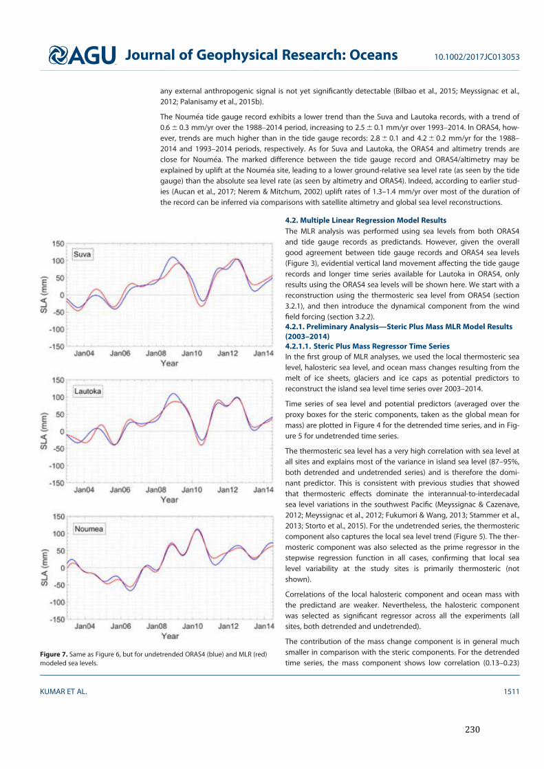
230

any external anthropogenic signal is not yet significantly detectable (Bilbao et al., 2015; Meyssignac et al.,2012; Palanisamy et al., 2015b).

The Noum!ea tide gauge record exhibits a lower trend than the Suva and Lautoka records, with a trend of0.6 6 0.3 mm/yr over the 1988–2014 period, increasing to 2.5 6 0.1 mm/yr over 1993–2014. In ORAS4, how-ever, trends are much higher than in the tide gauge records: 2.8 6 0.1 and 4.2 6 0.2 mm/yr for the 1988–2014 and 1993–2014 periods, respectively. As for Suva and Lautoka, the ORAS4 and altimetry trends areclose for Noum!ea. The marked difference between the tide gauge record and ORAS4/altimetry may beexplained by uplift at the Noum!ea site, leading to a lower ground-relative sea level rate (as seen by the tidegauge) than the absolute sea level rate (as seen by altimetry and ORAS4). Indeed, according to earlier stud-ies (Aucan et al., 2017; Nerem & Mitchum, 2002) uplift rates of 1.3–1.4 mm/yr over most of the duration ofthe record can be inferred via comparisons with satellite altimetry and global sea level reconstructions.

4.2. Multiple Linear Regression Model ResultsThe MLR analysis was performed using sea levels from both ORAS4and tide gauge records as predictands. However, given the overallgood agreement between tide gauge records and ORAS4 sea levels(Figure 3), evidential vertical land movement affecting the tide gaugerecords and longer time series available for Lautoka in ORAS4, onlyresults using the ORAS4 sea levels will be shown here. We start with areconstruction using the thermosteric sea level from ORAS4 (section3.2.1), and then introduce the dynamical component from the windfield forcing (section 3.2.2).4.2.1. Preliminary Analysis—Steric Plus Mass MLR Model Results(2003–2014)4.2.1.1. Steric Plus Mass Regressor Time SeriesIn the first group of MLR analyses, we used the local thermosteric sealevel, halosteric sea level, and ocean mass changes resulting from themelt of ice sheets, glaciers and ice caps as potential predictors toreconstruct the island sea level time series over 2003–2014.

Time series of sea level and potential predictors (averaged over theproxy boxes for the steric components, taken as the global mean formass) are plotted in Figure 4 for the detrended time series, and in Fig-ure 5 for undetrended time series.

The thermosteric sea level has a very high correlation with sea level atall sites and explains most of the variance in island sea level (87–95%,both detrended and undetrended series) and is therefore the domi-nant predictor. This is consistent with previous studies that showedthat thermosteric effects dominate the interannual-to-interdecadalsea level variations in the southwest Pacific (Meyssignac & Cazenave,2012; Meyssignac et al., 2012; Fukumori & Wang, 2013; Stammer et al.,2013; Storto et al., 2015). For the undetrended series, the thermostericcomponent also captures the local sea level trend (Figure 5). The ther-mosteric component was also selected as the prime regressor in thestepwise regression function in all cases, confirming that local sealevel variability at the study sites is primarily thermosteric (notshown).

Correlations of the local halosteric component and ocean mass withthe predictand are weaker. Nevertheless, the halosteric componentwas selected as significant regressor across all the experiments (allsites, both detrended and undetrended).

The contribution of the mass change component is in general muchsmaller in comparison with the steric components. For the detrendedtime series, the mass component shows low correlation (0.13–0.23)

Figure 7. Same as Figure 6, but for undetrended ORAS4 (blue) and MLR (red)modeled sea levels.


KUMAR ET AL. 1511

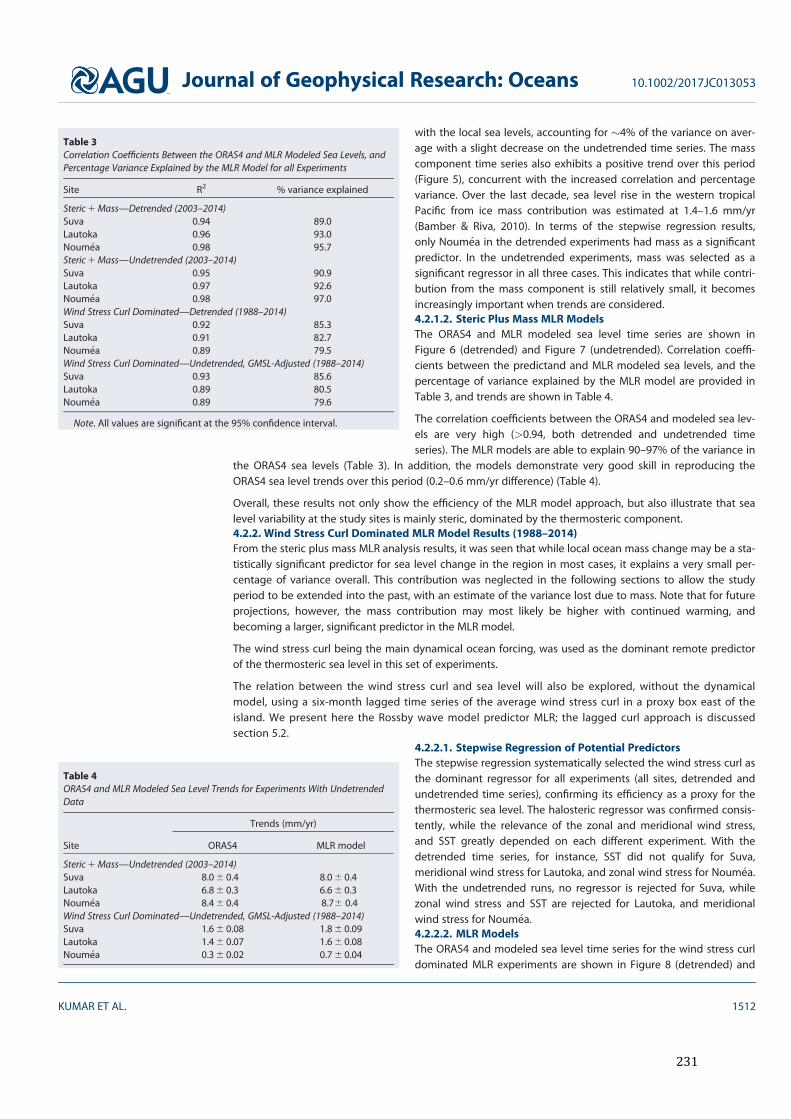
231

with the local sea levels, accounting for !4% of the variance on aver-age with a slight decrease on the undetrended time series. The masscomponent time series also exhibits a positive trend over this period(Figure 5), concurrent with the increased correlation and percentagevariance. Over the last decade, sea level rise in the western tropicalPacific from ice mass contribution was estimated at 1.4–1.6 mm/yr(Bamber & Riva, 2010). In terms of the stepwise regression results,only Noum!ea in the detrended experiments had mass as a significantpredictor. In the undetrended experiments, mass was selected as asignificant regressor in all three cases. This indicates that while contri-bution from the mass component is still relatively small, it becomesincreasingly important when trends are considered.4.2.1.2. Steric Plus Mass MLR ModelsThe ORAS4 and MLR modeled sea level time series are shown inFigure 6 (detrended) and Figure 7 (undetrended). Correlation coeffi-cients between the predictand and MLR modeled sea levels, and thepercentage of variance explained by the MLR model are provided inTable 3, and trends are shown in Table 4.

The correlation coefficients between the ORAS4 and modeled sea lev-els are very high (>0.94, both detrended and undetrended timeseries). The MLR models are able to explain 90–97% of the variance in

the ORAS4 sea levels (Table 3). In addition, the models demonstrate very good skill in reproducing theORAS4 sea level trends over this period (0.2–0.6 mm/yr difference) (Table 4).

Overall, these results not only show the efficiency of the MLR model approach, but also illustrate that sealevel variability at the study sites is mainly steric, dominated by the thermosteric component.4.2.2. Wind Stress Curl Dominated MLR Model Results (1988–2014)From the steric plus mass MLR analysis results, it was seen that while local ocean mass change may be a sta-tistically significant predictor for sea level change in the region in most cases, it explains a very small per-centage of variance overall. This contribution was neglected in the following sections to allow the studyperiod to be extended into the past, with an estimate of the variance lost due to mass. Note that for futureprojections, however, the mass contribution may most likely be higher with continued warming, andbecoming a larger, significant predictor in the MLR model.

The wind stress curl being the main dynamical ocean forcing, was used as the dominant remote predictorof the thermosteric sea level in this set of experiments.

The relation between the wind stress curl and sea level will also be explored, without the dynamicalmodel, using a six-month lagged time series of the average wind stress curl in a proxy box east of theisland. We present here the Rossby wave model predictor MLR; the lagged curl approach is discussedsection 5.2.

4.2.2.1. Stepwise Regression of Potential PredictorsThe stepwise regression systematically selected the wind stress curl asthe dominant regressor for all experiments (all sites, detrended andundetrended time series), confirming its efficiency as a proxy for thethermosteric sea level. The halosteric regressor was confirmed consis-tently, while the relevance of the zonal and meridional wind stress,and SST greatly depended on each different experiment. With thedetrended time series, for instance, SST did not qualify for Suva,meridional wind stress for Lautoka, and zonal wind stress for Noum!ea.With the undetrended runs, no regressor is rejected for Suva, whilezonal wind stress and SST are rejected for Lautoka, and meridionalwind stress for Noum!ea.4.2.2.2. MLR ModelsThe ORAS4 and modeled sea level time series for the wind stress curldominated MLR experiments are shown in Figure 8 (detrended) and

Table 3Correlation Coefficients Between the ORAS4 and MLR Modeled Sea Levels, andPercentage Variance Explained by the MLR Model for all Experiments

Site R2 % variance explained

Steric 1 Mass—Detrended (2003–2014)Suva 0.94 89.0Lautoka 0.96 93.0Noum!ea 0.98 95.7Steric 1 Mass—Undetrended (2003–2014)Suva 0.95 90.9Lautoka 0.97 92.6Noum!ea 0.98 97.0Wind Stress Curl Dominated—Detrended (1988–2014)Suva 0.92 85.3Lautoka 0.91 82.7Noum!ea 0.89 79.5Wind Stress Curl Dominated—Undetrended, GMSL-Adjusted (1988–2014)Suva 0.93 85.6Lautoka 0.89 80.5Noum!ea 0.89 79.6

Note. All values are significant at the 95% confidence interval.

Table 4ORAS4 and MLR Modeled Sea Level Trends for Experiments With UndetrendedData

Site

Trends (mm/yr)

ORAS4 MLR model

Steric 1 Mass—Undetrended (2003–2014)Suva 8.0 6 0.4 8.0 6 0.4Lautoka 6.8 6 0.3 6.6 6 0.3Noum!ea 8.4 6 0.4 8.76 0.4Wind Stress Curl Dominated—Undetrended, GMSL-Adjusted (1988–2014)Suva 1.6 6 0.08 1.8 6 0.09Lautoka 1.4 6 0.07 1.6 6 0.08Noum!ea 0.3 6 0.02 0.7 6 0.04


KUMAR ET AL. 1512

232

with the local sea levels, accounting for !4% of the variance on aver-age with a slight decrease on the undetrended time series. The masscomponent time series also exhibits a positive trend over this period(Figure 5), concurrent with the increased correlation and percentagevariance. Over the last decade, sea level rise in the western tropicalPacific from ice mass contribution was estimated at 1.4–1.6 mm/yr(Bamber & Riva, 2010). In terms of the stepwise regression results,only Noum!ea in the detrended experiments had mass as a significantpredictor. In the undetrended experiments, mass was selected as asignificant regressor in all three cases. This indicates that while contri-bution from the mass component is still relatively small, it becomesincreasingly important when trends are considered.4.2.1.2. Steric Plus Mass MLR ModelsThe ORAS4 and MLR modeled sea level time series are shown inFigure 6 (detrended) and Figure 7 (undetrended). Correlation coeffi-cients between the predictand and MLR modeled sea levels, and thepercentage of variance explained by the MLR model are provided inTable 3, and trends are shown in Table 4.

The correlation coefficients between the ORAS4 and modeled sea lev-els are very high (>0.94, both detrended and undetrended timeseries). The MLR models are able to explain 90–97% of the variance in

the ORAS4 sea levels (Table 3). In addition, the models demonstrate very good skill in reproducing theORAS4 sea level trends over this period (0.2–0.6 mm/yr difference) (Table 4).

Overall, these results not only show the efficiency of the MLR model approach, but also illustrate that sealevel variability at the study sites is mainly steric, dominated by the thermosteric component.4.2.2. Wind Stress Curl Dominated MLR Model Results (1988–2014)From the steric plus mass MLR analysis results, it was seen that while local ocean mass change may be a sta-tistically significant predictor for sea level change in the region in most cases, it explains a very small per-centage of variance overall. This contribution was neglected in the following sections to allow the studyperiod to be extended into the past, with an estimate of the variance lost due to mass. Note that for futureprojections, however, the mass contribution may most likely be higher with continued warming, andbecoming a larger, significant predictor in the MLR model.

The wind stress curl being the main dynamical ocean forcing, was used as the dominant remote predictorof the thermosteric sea level in this set of experiments.

The relation between the wind stress curl and sea level will also be explored, without the dynamicalmodel, using a six-month lagged time series of the average wind stress curl in a proxy box east of theisland. We present here the Rossby wave model predictor MLR; the lagged curl approach is discussedsection 5.2.

4.2.2.1. Stepwise Regression of Potential PredictorsThe stepwise regression systematically selected the wind stress curl asthe dominant regressor for all experiments (all sites, detrended andundetrended time series), confirming its efficiency as a proxy for thethermosteric sea level. The halosteric regressor was confirmed consis-tently, while the relevance of the zonal and meridional wind stress,and SST greatly depended on each different experiment. With thedetrended time series, for instance, SST did not qualify for Suva,meridional wind stress for Lautoka, and zonal wind stress for Noum!ea.With the undetrended runs, no regressor is rejected for Suva, whilezonal wind stress and SST are rejected for Lautoka, and meridionalwind stress for Noum!ea.4.2.2.2. MLR ModelsThe ORAS4 and modeled sea level time series for the wind stress curldominated MLR experiments are shown in Figure 8 (detrended) and

Table 3Correlation Coefficients Between the ORAS4 and MLR Modeled Sea Levels, andPercentage Variance Explained by the MLR Model for all Experiments

Site R2 % variance explained

Steric 1 Mass—Detrended (2003–2014)Suva 0.94 89.0Lautoka 0.96 93.0Noum!ea 0.98 95.7Steric 1 Mass—Undetrended (2003–2014)Suva 0.95 90.9Lautoka 0.97 92.6Noum!ea 0.98 97.0Wind Stress Curl Dominated—Detrended (1988–2014)Suva 0.92 85.3Lautoka 0.91 82.7Noum!ea 0.89 79.5Wind Stress Curl Dominated—Undetrended, GMSL-Adjusted (1988–2014)Suva 0.93 85.6Lautoka 0.89 80.5Noum!ea 0.89 79.6


Table 4ORAS4 and MLR Modeled Sea Level Trends for Experiments With UndetrendedData

Site

Trends (mm/yr)

ORAS4 MLR model

Steric 1 Mass—Undetrended (2003–2014)Suva 8.0 6 0.4 8.0 6 0.4Lautoka 6.8 6 0.3 6.6 6 0.3Noum!ea 8.4 6 0.4 8.76 0.4Wind Stress Curl Dominated—Undetrended, GMSL-Adjusted (1988–2014)Suva 1.6 6 0.08 1.8 6 0.09Lautoka 1.4 6 0.07 1.6 6 0.08Noum!ea 0.3 6 0.02 0.7 6 0.04


KUMAR ET AL. 1512

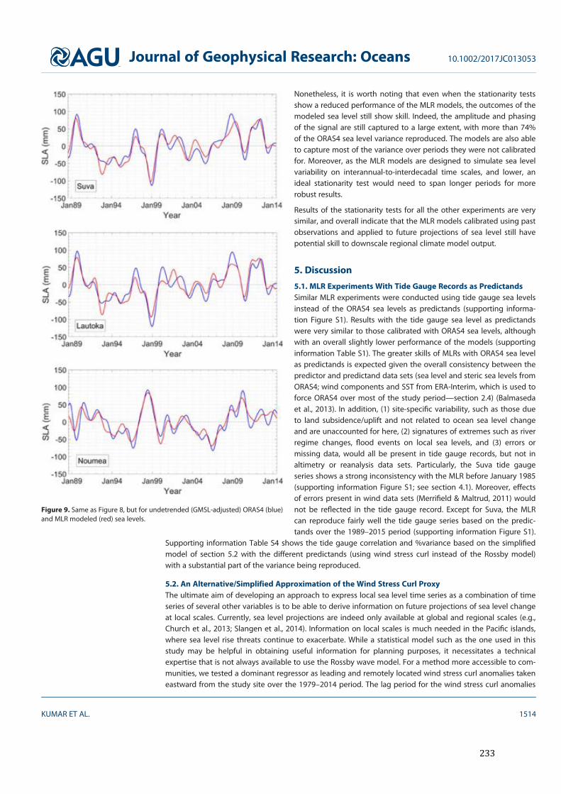
233

Nonetheless, it is worth noting that even when the stationarity testsshow a reduced performance of the MLR models, the outcomes of themodeled sea level still show skill. Indeed, the amplitude and phasingof the signal are still captured to a large extent, with more than 74%of the ORAS4 sea level variance reproduced. The models are also ableto capture most of the variance over periods they were not calibratedfor. Moreover, as the MLR models are designed to simulate sea levelvariability on interannual-to-interdecadal time scales, and lower, anideal stationarity test would need to span longer periods for morerobust results.

Results of the stationarity tests for all the other experiments are verysimilar, and overall indicate that the MLR models calibrated using pastobservations and applied to future projections of sea level still havepotential skill to downscale regional climate model output.

5. Discussion

5.1. MLR Experiments With Tide Gauge Records as PredictandsSimilar MLR experiments were conducted using tide gauge sea levelsinstead of the ORAS4 sea levels as predictands (supporting informa-tion Figure S1). Results with the tide gauge sea level as predictandswere very similar to those calibrated with ORAS4 sea levels, althoughwith an overall slightly lower performance of the models (supportinginformation Table S1). The greater skills of MLRs with ORAS4 sea levelas predictands is expected given the overall consistency between thepredictor and predictand data sets (sea level and steric sea levels fromORAS4; wind components and SST from ERA-Interim, which is used toforce ORAS4 over most of the study period—section 2.4) (Balmasedaet al., 2013). In addition, (1) site-specific variability, such as those dueto land subsidence/uplift and not related to ocean sea level changeand are unaccounted for here, (2) signatures of extremes such as riverregime changes, flood events on local sea levels, and (3) errors ormissing data, would all be present in tide gauge records, but not inaltimetry or reanalysis data sets. Particularly, the Suva tide gaugeseries shows a strong inconsistency with the MLR before January 1985(supporting information Figure S1; see section 4.1). Moreover, effectsof errors present in wind data sets (Merrifield & Maltrud, 2011) wouldnot be reflected in the tide gauge record. Except for Suva, the MLRcan reproduce fairly well the tide gauge series based on the predic-tands over the 1989–2015 period (supporting information Figure S1).

Supporting information Table S4 shows the tide gauge correlation and %variance based on the simplifiedmodel of section 5.2 with the different predictands (using wind stress curl instead of the Rossby model)with a substantial part of the variance being reproduced.

5.2. An Alternative/Simplified Approximation of the Wind Stress Curl ProxyThe ultimate aim of developing an approach to express local sea level time series as a combination of timeseries of several other variables is to be able to derive information on future projections of sea level changeat local scales. Currently, sea level projections are indeed only available at global and regional scales (e.g.,Church et al., 2013; Slangen et al., 2014). Information on local scales is much needed in the Pacific islands,where sea level rise threats continue to exacerbate. While a statistical model such as the one used in thisstudy may be helpful in obtaining useful information for planning purposes, it necessitates a technicalexpertise that is not always available to use the Rossby wave model. For a method more accessible to com-munities, we tested a dominant regressor as leading and remotely located wind stress curl anomalies takeneastward from the study site over the 1979–2014 period. The lag period for the wind stress curl anomalies

Figure 9. Same as Figure 8, but for undetrended (GMSL-adjusted) ORAS4 (blue)and MLR modeled (red) sea levels.


KUMAR ET AL. 1514

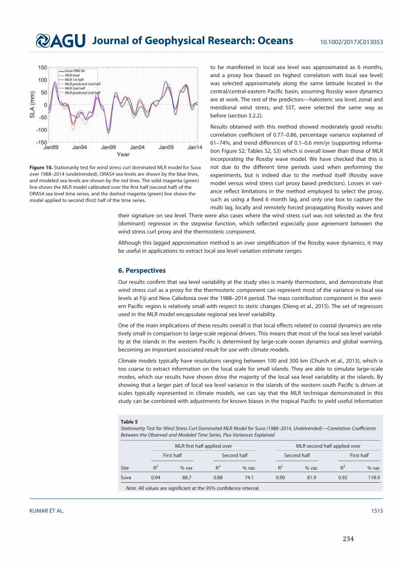
234

to be manifested in local sea level was approximated as 6 months,and a proxy box (based on highest correlation with local sea level)was selected approximately along the same latitude located in thecentral/central-eastern Pacific basin, assuming Rossby wave dynamicsare at work. The rest of the predictors—halosteric sea level, zonal andmeridional wind stress, and SST, were selected the same way asbefore (section 3.2.2).

Results obtained with this method showed moderately good results:correlation coefficient of 0.77–0.86, percentage variance explained of61–74%, and trend differences of 0.1–0.6 mm/yr (supporting informa-tion Figure S2; Tables S2, S3) which is overall lower than those of MLRincorporating the Rossby wave model. We have checked that this isnot due to the different time periods used when performing theexperiments, but is indeed due to the method itself (Rossby wavemodel versus wind stress curl proxy based predictors). Losses in vari-ance reflect limitations in the method employed to select the proxy,such as using a fixed 6 month lag, and only one box to capture themulti lag, locally and remotely forced propagating Rossby waves and

their signature on sea level. There were also cases where the wind stress curl was not selected as the first(dominant) regressor in the stepwise function, which reflected especially poor agreement between thewind stress curl proxy and the thermosteric component.

Although this lagged approximation method is an over simplification of the Rossby wave dynamics, it maybe useful in applications to extract local sea level variation estimate ranges.

6. Perspectives

Our results confirm that sea level variability at the study sites is mainly thermosteric, and demonstrate thatwind stress curl as a proxy for the thermosteric component can represent most of the variance in local sealevels at Fiji and New Caledonia over the 1988–2014 period. The mass contribution component in the west-ern Pacific region is relatively small with respect to steric changes (Dieng et al., 2015). The set of regressorsused in the MLR model encapsulate regional sea level variability.

One of the main implications of these results overall is that local effects related to coastal dynamics are rela-tively small in comparison to large-scale regional drivers. This means that most of the local sea level variabil-ity at the islands in the western Pacific is determined by large-scale ocean dynamics and global warming,becoming an important associated result for use with climate models.

Climate models typically have resolutions ranging between 100 and 300 km (Church et al., 2013), which istoo coarse to extract information on the local scale for small islands. They are able to simulate large-scalemodes, which our results have shown drive the majority of the local sea level variability at the islands. Byshowing that a larger part of local sea level variance in the islands of the western south Pacific is driven atscales typically represented in climate models, we can say that the MLR technique demonstrated in thisstudy can be combined with adjustments for known biases in the tropical Pacific to yield useful information

Figure 10. Stationarity test for wind stress curl dominated MLR model for Suvaover 1988–2014 (undetrended). ORAS4 sea levels are shown by the blue lines,and modeled sea levels are shown by the red lines. The solid magenta (green)line shows the MLR model calibrated over the first half (second half) of theORAS4 sea level time series, and the dashed magenta (green) line shows themodel applied to second (first) half of the time series.

Table 5Stationarity Test for Wind Stress Curl Dominated MLR Model for Suva (1988–2014, Undetrended)—Correlation CoefficientsBetween the Observed and Modeled Time Series, Plus Variances Explained

Site

MLR first half applied over MLR second half applied over

First half Second half Second half First half

R2 % var. R2 % var. R2 % var. R2 % var.

Suva 0.94 88.7 0.88 74.1 0.90 81.9 0.92 118.9



KUMAR ET AL. 1515

235

at local scales through downscaling studies. Furthermore, the mechanistic approach adopted in developingthe MLR model might be more consistent for downscaling climate model simulations than directly usingthe local thermosteric components.

However, it must be recognized that climate models have inherent biases in the tropical Pacific region, suchas the double Intertropical Convergence Zone (ITCZ)/zonal South Pacific Convergence zone (SPCZ), and thewestward extension of the equatorial cold tongue (Flato et al., 2013). Simulations of sea surface tempera-tures and sea level are connected to the representation of dynamical processes and key regional featuressuch as those described over the water column, and hence have resultant biases as well. Further uncertain-ties in climate model simulations exist due to limitations in parameterizations of complex or unresolvedphysical processes (Church et al., 2013; Flato et al., 2013; Melet et al., 2016b). Thus, these models must beused with caution for practical planning by island agencies.

Furthermore, the dynamical Rossby MLR model might be more consistent for downscaling climate modelsimulations than directly using the local thermosteric components, which may be affected by local biases.

Our MLR technique provides a better understanding of key physical drivers of sea level variability in islandsin the region, and can be applied to other regions, with some adaptation to site-specific dominant drivers/modes (e.g., Sprintall & R!evelard, 2014; Sterlini et al., 2016). Additionally, vertical land motion affecting localsea levels would need be taken in account if relevant, as the model regressors considered here do notinclude it. Local scale information obtained from such studies will be greatly valuable in developing efficientrisk minimization measures, and planning effective adaptation techniques in areas threated by sea levelrise.

ReferencesAlbert, S., Leon, J. X., Grinham, A. R., Church, J. A., Gibbes, B. R., & Woodroffe, C. D. (2016). Interactions between sea-level rise and wave

exposure on reef island dynamics in the Solomon Islands. Environmental Research Letters, 11, 054011. https://doi.org/10.1088/1748–9326/11/5/054011

Aucan, J., Merrifield, M. A., & Pouvreau, N. (2017). Historical sea-level measurements in the South Pacific from rescued archive, geodeticmeasurements and satellite altimetry. Pure and Applied Geophysics, 174, 3813–3823. https://doi.org/10.1007/s00024-017-1648-1

Ballu, V., Bouin, M.-N., Simeoni, P., Crawford, W. C., Calmant, S., Bore, J.-M., et al. (2011). Comparing the role of absolute sea-level rise andvertical tectonic motions in coastal flooding, Torres Islands (Vanuatu). Proceedings of the National Academy of Sciences of the UnitedStates of America, 108, 13019–13022. https://doi.org/10.1073/pnas.1102842108

Balmaseda, M. A., Hernandez, F., Storto, A., Palmer, M. D., Alves, O., Shi, L., et al. (2015). The Ocean Reanalyses Intercomparison Project(ORA-IP). Journal of Operational Oceanography, 8, s80–s97. https://doi.org/10.1080/1755876X.2015.1022329

Balmaseda, M. A., Mogensen, K., & Weaver, A. T. (2013). Evaluation of the ECMWF ocean reanalysis system ORAS4. Quarterly Journal of theRoyal Meteorological Society, 139, 1132–1161. https://doi.org/10.1002/qj.2063

Bamber, J., & Riva, R. (2010). The sea-level fingerprint of recent ice mass fluxes. Cryosphere, 4, 621–627. https://doi.org/10.5194/tc-4-621-2010Barnett, J., & Campbell, J. (2010). Climate change and small island states—Power, Knowledge and the South Pacific (217 p.). London, UK:

Earthscan.Becker, M., Karpytchev, M., & Lennartz-Sassinek, S. (2014). Long-term sea-level trends—Natural or Antropogenic? Geophysical Research Let-

ters, 41, 557–5580. https:/doi.org/10.1002/2014GL061027Becker, M., Meyssignac, B., Letetrel, C., Llovel, W., Cazenave, A., & Delcroix, T. (2012). Sea level variations at tropical Pacific islands since

1950. Global and Planetary Change, 80–81, 85–98. https://doi.org/10.1016/j.gloplacha.2011.09.004Bilbao, R. A. F., Gregory, J. M., & Bouttes, N. (2015). Analysis of the regional pattern of sea-level change due to ocean dynamics and density

change for 1993–2099 in observations and CMIP5 AOGCMs. Climate Dynamics, 45, 2647–2666. https://doi.org/10.1007/s00382-015-2499-z

Bromirski, P. D., Miller, A. J., Flick, R. E., & Auad, G. (2011). Dynamical suppression of sea-level rise along the Pacific coast of North America:Indications for imminent acceleration. Journal of Geophysical Research, 116, C07005. https://doi.org/10.1029/2010JC006759

Carret, A., Johannessen, J. A., Anderson, O. B., Ablain, M., Prandi, P., Blazquez, A., & Cazenave, A. (2016). Arctic sea level during the satellitealtimetry era. Surveys in Geophysics, 38, 251–275. https://doi.org/10.1007/s10712-016-9390-2

Carton, J. A., Giese, B. S., & Grodsky, S. A. (2005). Sea-level rise and the warming of the oceans in the Simple Ocean Data Assimilation(SODA) ocean reanalysis. Journal of Geophysical Research, 110, C09006. https://doi.org/10.1029/2004JC002817

Cazenave, A., & Llovel, W. (2010). Contemporary sea-level rise. Annual Review of Marine Science, 2, 145–173.Church, J. A., Clark, P. U., Cazenave, A., Gregory, J. M., Jevrejeva, S., Levermann, A., et al. (2013). Sea-level change. In T. F. Stocker et al. (Eds.),

Climate change 2013a: The physical science basis. Contribution of working group I to the fifth assessment report of the intergovernmentalpanel on climate change. Cambridge, UK: Cambridge University Press.

Church, J. A., Gregory, J., White, N., Platten, S., & Mitrovica, J. (2011). Understanding and projecting sea-level change. Oceanography, 24,130–143. https://doi.org/10.5670/oceanog.2011.33

Church, J. A., & White, N. J. (2011). Sea-Level Rise from the Late 19th to the Early 21st Century. Surveys in Geophysics, 32, 585–602. https://doi.org/10.1007/s10712-011-9119-1

CMEMS (2016). Retrieved from http://marine.copernicus.eu/, accessed 20 January 2016.Dee, D. P., Uppala, S. M., Simmons, A. J., Berrisford, P., Poli, P., Kobayashi, S., et al. (2011). The ERA-Interim reanalysis: Configuration and perfor-

mance of the data assimilation system. Quarterly Journal of the Royal Meteorological Society, 137, 553–597. https://doi.org/10.1002/qj.828

AcknowledgmentsWe wish to thank the IPCC and the IRDfor conjointly funding this researchproject as part of V. Kumar’s PhD. Thedata used here are listed in thereferences and repositories cited. Thisis contribution number 4712 from thePacific Marine EnvironmentalLaboratory/NOAA. This work has beensupported by CNES. Some of the datapresented here is based on dataretreived by the CNES/NASA missionsTopex, Jason 1,2 and 3. It has beenconducted using E.U. CopernicusMarine Service information.


KUMAR ET AL. 1516

236

Dieng, H. B., Champollion, N., Cazenave, A., Wada, Y., Schrama, E., & Meyssignac, B. (2015). Total land water storage change over 2003–2013 esti-mated from a global mass budget approach. Environmental Research Letters, 10, 124010. https://doi.org/10.1088/1748-9326/10/12/124010

ERA-Interim (2016). Retrieved from http://www.ecmwf.int/en/research/climate-reanalysis/era-interim, accessed 2 March 2016.Flato, G., Marotzke, J., Abiodun, B., Braconnot, P., Chou, S. C., Collins, W., et al. (2013). Evaluation of climate models. In T. F. Stocker et al.

(Eds.), Climate change 2013: The physical science basis. Contribution of working group I to the fifth assessment report of the intergovernmen-tal panel on climate change. Cambridge, UK: Cambridge University Press.

Forget, G., & Ponte, R. M. (2015). The partition of regional sea-level variability. Progress in Oceanography, 137, 173–195. https://doi.org/10.1016/j.pocean.2015.06.002

Fukumori, I., & Wang, O. (2013). Origins of heat and freshwater anomalies underlying regional decadal sea-level trends: Regional decadalsea-level trends. Geophysical Research Letters, 40, 563–567. https://doi.org/10.1002/grl.50164

Garschagen, M., Hagenlocher, M., Sabelfeld, R., & Lee, Y. J. (2016). Infrastructure as a risk factor. In L. Jeschonnek et al. (Eds.), World riskreport 2016 (pp. 14–21). Berlin, Germany: B€undnis Entwicklung Hilft (Alliance Development Works); United Nations University—Institutefor Environment and Human Security (UNU-EHS).

Gregory, J. M., & Lowe, J. A. (2000). Predictions of global and regional sea-level rise using AOGCMs with and without flux adjustment. Geo-physical Research Letters, 27, 3069–3072.

Hallegatte, S., Green, C., Nicholls, R. J., & Corfee-Morlot, J. (2013). Future flood losses in major coastal cities. Nature Climate Change, 3, 802–806. https://doi.org/10.1038/nclimate1979

Hay, C. C., Morrow, E., Kopp, R. E., & Mitrovica, J. X. (2015). Probabilistic reanalysis of twentieth-century sea-level rise. Nature, 517, 481–84.https://doi.org/10.1038/nature14093

Holgate, S. J., Matthews, A., Woodworth, P. L., Rickards, L. J., Tamisiea, M. E., Bradshaw, E., et al. (2013). New data systems and products atthe permanent service for mean sea-level. Journal of Coastal Research, 288, 493–504. https://doi.org/10.2112/JCOASTRES-D-12-00175.1

Huang, R. X. (2015). Heaving modes in the world oceans. Climate Dynamics, 45, 3563–3591. https://doi.org/10.1007/s00382-015-2557-6Jevrejeva, S., Moore, J. C., Grinsted, A., & Woodworth, P. L. (2008). Recent global sea-level acceleration started over 200 years ago? Geophys-

ical Research Letters, 35, L08715. https://doi.org/10.1029/2008GL033611Kessler, W. S., & Cravatte, S. (2013). ENSO and short-term variability of the South Equatorial current entering the Coral sea. Journal of Physi-

cal Oceanography, 43, 956–969. https://doi.org/10.1175/JPO-D-12-0113.1K€ohl, A., Stammer, D., & Cornuelle, B. (2007). Interannual to decadal changes in the ECCO global synthesis. Journal of Physical Oceanogra-

phy, 37, 313–337. https://doi.org/10.1175/JPO3014.1Levitus, S., Antonov, J. I., Boyer, T. P., Baranova, O. K., Garcia, H. E., Locarnini, R. A., et al. (2012). World ocean heat content and thermosteric

sea-level change (0–2000 m), 1955–2010. Geophysical Research Letters, 39, L10603. https://doi.org/10.1029/2012GL051106Levitus, S., Antonov, J. I., Boyer, T. P., Garcia, H. E., & Locarnini, R. A. (2005). Linear trends of zonally averaged thermosteric, halosteric, and

total steric sea-level for individual ocean basins and the world ocean, (1955–1959)–(1994–1998). Geophysical Research Letters, 32,L16601. https://doi.org/10.1029/2005GL023761

Levitus, S., Antonov, J. I., Boyer, T. P., Locarnini, R. A., Garcia, H. E., & Mishonov, A. V. (2009). Global ocean heat content 1955–2008 in light ofrecently revealed instrumentation problems. Geophysical Research Letters, 36, L07608. https://doi.org/10.1029/2008GL037155

Lombard, A., Cazenave, A., Le Traon, P.-Y., & Ishii, M. (2005). Contribution of thermal expansion to present-day sea-level change revisited.Global and Planetary Change, 47, 1–16. https://doi.org/10.1016/j.gloplacha.2004.11.016

Lombard, A., Garric, G., & Penduff, T. (2009). Regional patterns of observed sea-level change: Insights from a 1/48 global ocean/sea-ice hind-cast. Ocean Dynamics, 59, 433–449. https://doi.org/10.1007/s10236-008-0161-6

McDougall, T. J., & Barker, P. M. (2011). Getting started with TEOS-10 and the Gibbs Seawater (GSW) Oceanographic Toolbox. Version 3.05.5(SCOR/IAPSO WG127, 28 p.).

McGregor, S., Gupta, A. S., & England, M. H. (2012). Constraining wind stress products with sea surface height observations and implicationsfor Pacific Ocean sea-level trend attribution. Journal of Climate, 25, 8164–8176.

McNamara, K. E., & Jacot Des Combes, H. (2015). Planning for community relocations due to climate change in Fiji. International Journal ofDisaster Risk Science, 6, 315–319. https://doi.org/10.1007/s13753-015-0065-2

Melet, A., Almar, R., & Meyssignac, B. (2016a). What dominates sea-level at the coast: A case study for the Gulf of Guinea. Ocean Dynamics,66, 623–636. https://doi.org/10.1007/s10236-016-0942-2

Melet, A., Legg, S., & Hallberg, R. (2016b). Climatic impacts of parameterized local and remote tidal mixing. Journal of Climate, 29, 3473–3500. https://doi.org/10.1175/JCLI-D-15-0153.1

Merrifield, M. A. (2011). A shift in Western Tropical Pacific sea-level trends during the 1990s. Journal of Climate, 24, 4126–4138. https://doi.org/10.1175/2011JCLI3932.1

Merrifield, M. A., & Maltrud, M. E. (2011). Regional sea-level trends due to a Pacific trade wind intensification. Geophysical Research Letters,38, L21605. https://doi.org/10.1029/2011GL049576

Merrifield, M. A., Thompson, P. R., & Lander, M. (2012). Multidecadal sea-level anomalies and trends in the western tropical Pacific. Geophys-ical Research Letters, 39, L13602. https://doi.org/10.1029/2012GL052032

Meyssignac, B., & Cazenave, A. (2012). Sea-level: A review of present-day and recent-past changes and variability. Journal of Geodynamics,58, 96–109. https://doi.org/10.1016/j.jog.2012.03.005

Meyssignac, B., Piecuch, C. G., Merchant, C. J., Racault, M.-F., Palanisamy, H., MacIntosh, C., et al. (2017). Causes of the regional variability inobserved sea-level, sea surface temperature and ocean colour over the period 1993–2011. Surveys in Geophysics, 38, 187–215. https://doi.org/10.1007/s10712-016-9383-1

Meyssignac, B., Salas, D., Melia, M., Becker, W., Llovel, & Cazenave, A. (2012). Tropical Pacific spatial trend patterns in observed sea-level:Internal variability and/or anthropogenic signature? Climate of the Past, 8, 787–802. https://doi.org/10.5194/cp-8-787-2012

Milne, G. A., Gehrels, W., Hughes, C., & Tamisiea, M. (2009). Identifying the causes of sea-level change. Nature Geoscience, 2, 471–478.Mimura, N. (1999). Vulnerability of island countries in the South Pacific to sea-level rise and climate change. Climate Research, 12, 137–143.Mitrovica, J. X., Gomez, N., & Clark, P. U. (2009). The sea-level fingerprint of West Antarctic Collapse. Science, 323, 753–753. https://doi.org/

10.1126/science.1166510Mitrovica, J. X., Gomez, N., Morrow, E., Hay, C., Latychev, K., & Tamisiea, M. E. (2011). On the robustness of predictions of sea-level finger-

prints: On predictions of sea-level fingerprints. Geophysical Journal International, 187, 729–742. https://doi.org/10.1111/j.1365-246X.2011.05090.x

Nerem, R. S., Chambers, D. P., Choe, C., & Mitchum, G. T. (2010). Estimating mean sea-level change from the TOPEX and Jason AltimeterMissions. Marine Geodynamics, 33, 435–446.


KUMAR ET AL. 1517

237

Nerem, R. S., & Mitchum, G. T. (2002). Estimates of vertical crustal motion derived from differences of TOPEX/POSEIDON and tide gauge sealevel measurements. Geophysical Research Letters, 29(19), 1934. https://doi.org/10.1029/2002GL015037

Neumann, B., Vafeidis, A. T., Zimmermann, J., & Nicholls, R. J. (2015). Future coastal population growth and exposure to sea-level rise andcoastal flooding—A global assessment. Plos One, 10, e0118571. https://doi.org/10.1371/journal.pone.0118571

Nidheesh, A. G., Lengaigne, M., Vialard, J., Unnikrishnan, A. S., & Dayan, H. (2013). Decadal and long-term sea-level variability in the tropicalIndo-Pacific Ocean. Climate Dynamics, 41, 381–402. https://doi.org/10.1007/s00382-012-1463-4

Nurse, L. A., McLean, R. F., Agard, J., Briguglio, L. P., Duvat-Magnan, V., Pelesikoti, N., et al. (2014). Small islands. In V. R. Barros et al. (Eds.), Cli-mate xhange 2014: Impacts, adaptation, and vulnerability. Part B: Regional aspects. Contribution of working group II to the Fifth AssessmentReport Of The Intergovernmental Panel On Climate Change (pp. 1613–1654). Cambridge, UK: Cambridge University Press.

OCHA—United Nations (2014). Fiji: Building resilience in the face of climate change. New York, NY: United Nations Office forthe Coordination of Humanitarian Affairs. Retrieved from http://www.unocha.org/top-stories/all-stories/fiji-building-resilience-face-cli-mate-change, accessed 16 October 2016.

Palanisamy, H., Cazenave, A., Delcroix, T., & Meyssignac, B. (2015a). Spatial trend patterns in the Pacific Ocean sea-level during the altimetryera: The contribution of thermocline depth change and internal climate variability. Ocean Dynamics, 65, 341–356. https://doi.org/10.1007/s10236-014-0805-7

Palanisamy, H., Meyssignac, B., Cazenave, A., & Delcroix, T. (2015b). Is anthropogenic sea-level fingerprint already detectable in the PacificOcean? Environmental Research Letters, 10, 84024. https://doi.org/10.1088/1748-9326/10/8/084024

Peltier, W. R. (2004). Global glacial isostasy and the surface of the ice-age Earth: The ICE-5G (VM2) model and GRACE. Annual Review ofEarth and Planetary Sciences, 32, 111–149. https://doi.org/10.1146/annurev.earth.32.082503.144359

Piecuch, C. G., & Ponte, R. M. (2011). Mechanisms of interannual steric sea-level variability. Geophysical Research Letters, 38, L15605. https://doi.org/10.1029/2011GL048440

PSMSL (2016). Retrieved from http://www.psmsl.org/, accessed 18 January 2016.Ray, R. D., & Douglas, B. C. (2011). Experiments in reconstructing twentieth-century sea-levels. Progress in Oceanography, 91, 496–515.

https://doi.org/10.1016/j.pocean.2011.07.021Singh, A., Delcroix, T., & Cravatte, S. (2011). Contrasting the flavors of El Ni~no-Southern Oscillation using sea surface salinity observations.

Journal of Geophysical Research, 116, C06016. https://doi.org/10.1029/2010JC006862Slangen, A. B. A., van de Wal, R. S. W., Wada, Y., & Vermeersen, L. L. A. (2014). Comparing tide gauge observations to regional patterns of

sea-level change. Earth System Dynamics, 5, 243–255. https://doi.org/10.5194/esd-5-243-2014Sprintall, J., & R!evelard, A. (2014). The Indonesian Throughflow response to Indo-Pacific climate variability: Indonesian throughflow climate

response. Journal of Geophysical Research: Oceans, 119, 1161–1175. https://doi.org/10.1002/2013JC009533Stammer, D., Cazenave, A., Ponte, R. M., & Tamisiea, M. E. (2013). Causes for contemporary regional sea-level changes. Annual Review of

Marine Science, 5, 21–46. https://doi.org/10.1146/annurev-marine-121211-172406Sterlini, P., Vries, H., & Katsman, C. (2016). Sea surface height variability in the North East Atlantic from satellite altimetry. Climate Dynamics,

1285–1302. https://doi.org/10.1007/s00382-015-2901-xStorto, A., Masina, S., Balmaseda, M., Guinehut, S., Xue, Y., Szekely, T., et al. (2015). Steric sea-level variability (1993–2010) in an ensemble of

ocean reanalyses and objective analyses. Climate Dynamics, 49(3), 709–729. https://doi.org/10.1007/s00382-015-2554-9Thompson, P. R., Merrifield, M. A., Wells, J. R., & Chang, C. M. (2014). Wind-driven coastal sea-level variability in the Northeast Pacific. Journal

of Climate, 27, 4733–4751. https://doi.org/10.1175/JCLI-D-13-00225.1Timmermann, A., McGregor, S., & Jin, F.-F. (2010). Wind effects on past and future regional sea-level trends in the Southern Indo-Pacific.

Journal of Climate, 23, 4429–4437. https://doi.org/10.1175/2010JCLI3519.1Webb, A. P., & Kench, P. S. (2010). The dynamic response of reef islands to sea-level rise: Evidence from multi-decadal analysis of island

change in the Central Pacific. Global and Planetary Change, 72, 234–246. https://doi.org/10.1016/j.gloplacha.2010.05.003Williams, J., & Hughes, C. W. (2013). The coherence of small island sea-level with the wider ocean: A model study. Ocean Science, 9, 111–

119. https://doi.org/10.5194/os-9-111-2013Wong, P. P., Losada, I. J., Gattuso, J.-P., Hinkel, J., Khattabi, A., McInnes, K. L., et al. (2014). Coastal systems and low-lying areas. In C. B. Field

et al. (Eds.), Climate change 2014: Impacts, adaptation, and vulnerability. Part A: Global and sectoral aspects. Contribution of working groupII to the fifth assessment report of the intergovernmental panel on climate change (pp. 361–409). Cambridge, UK: Cambridge UniversityPress.

Wunsch, C., & Stammer, D. (1997). Atmospheric loading and the oceanic ‘‘inverted barometer’’ effect. Reviews of Geophysics, 35, 79–107.https://doi.org/10.1029/96RG03037

Zhang, X., & Church, J. A. (2012). Sea-level trends, interannual and decadal variability in the Pacific Ocean: Pacific sea-level trend and vari-ability. Geophysical Research Letters, 39, L21701. https://doi.org/10.1029/2012GL053240


KUMAR ET AL. 1518

239

Annex 2

Poster presentations

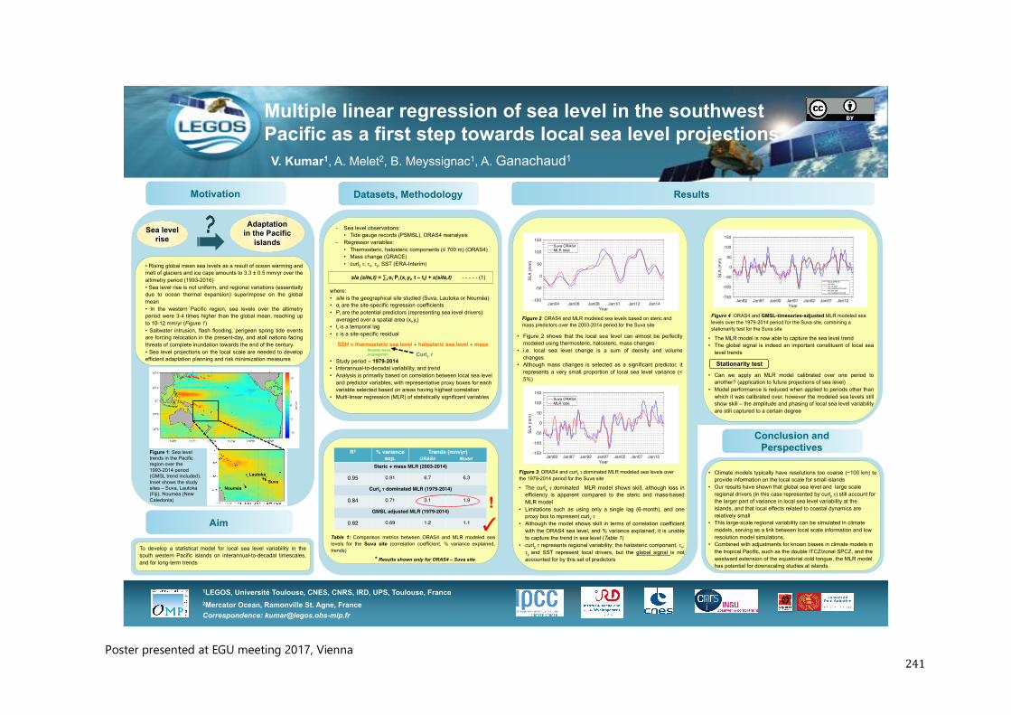
241

Multiple linear regression of sea level in the southwest Pacific as a first step towards local sea level projections

V. Kumar1, A. Melet2, B. Meyssignac1, A. Ganachaud1

Correspondence: [email protected]

1LEGOS, Université Toulouse, CNES, CNRS, IRD, UPS, Toulouse, France 2Mercator Ocean, Ramonville St. Agne, France

Sea level rise

Adaptation in the Pacific

islands

• Rising global mean sea levels as a result of ocean warming and melt of glaciers and ice caps amounts to 3.3 ± 0.5 mm/yr over the altimetry period (1993-2016) • Sea level rise is not uniform, and regional variations (essentially due to ocean thermal expansion) superimpose on the global mean • In the western Pacific region, sea levels over the altimetry period were 3-4 times higher than the global mean, reaching up to 10-12 mm/yr (Figure 1) • Saltwater intrusion, flash flooding, perigean spring tide events are forcing relocation in the present-day, and atoll nations facing threats of complete inundation towards the end of the century. • Sea level projections on the local scale are needed to develop efficient adaptation planning and risk minimization measures

Aim

To develop a statistical model for local sea level variability in the south western Pacific islands on interannual-to-decadal timescales, and for long-term trends

Motivation Datasets, Methodology Results

Figure 1: Sea level trends in the Pacific region over the 1993-2014 period (GMSL trend included). Inset shows the study sites – Suva, Lautoka (Fiji), Nouméa (New Caledonia)

Nouméa

Lautoka Suva

-  Sea level observations: •  Tide gauge records (PSMSL), ORAS4 reanalysis

-  Regressor variables: •  Thermosteric, halosteric components (≤ 700 m) (ORAS4) •  Mass change (GRACE) •  curlz τ, τx, τy, SST (ERA-Interim)

sla (site,t) = ∑I αi Pi (xi yi, t – ti) + ε(site,t) - - - - - (1) where: •  site is the geographical site studied (Suva, Lautoka or Nouméa) •  αi are the site-specific regression coefficients •  Pi are the potential predictors (representing sea level drivers)

averaged over a spatial area (xi,yi) •  ti is a temporal lag •  ε is a site-specific residual

SSH = thermosteric sea level + halosteric sea level + massRossby wave propagation Curlz τ

•  Study period – 1979-2014 •  Interannual-to-decadal variability, and trend •  Analysis is primarily based on correlation between local sea level

and predictor variables, with representative proxy boxes for each variable selected based on areas having highest correlation

•  Multi-linear regression (MLR) of statistically significant variables

R2 % variance exp.

Trends (mm/yr)

Steric + mass MLR (2003-2014)

0.95 0.91 6.7 6.3

Curlz τ dominated MLR (1979-2014)

0.84 0.71 3.1 1.9

GMSL adjusted MLR (1979-2014)

0.82 0.69 1.2 1.1

ORAS4 Model

!�

Table 1: Comparison metrics between ORAS4 and MLR modeled sea levels for the Suva site (correlation coefficient, % variance explained, trends)

YearJan04 Jan06 Jan08 Jan10 Jan12 Jan14

SLA

(mm

)

-100

-50

0

50

100

150Suva ORAS4MLR total

YearJan82 Jan87 Jan92 Jan97 Jan02 Jan07 Jan12

SLA

(mm

)

-150

-100

-50

0

50

100


Figure 2: ORAS4 and MLR modeled sea levels based on steric and mass predictors over the 2003-2014 period for the Suva site

•  Figure 2 shows that the local sea level can almost be perfectly modeled using thermosteric, halosteric, mass changes

•  i.e. local sea level change is a sum of density and volume changes

•  Although mass changes is selected as a significant predictor, it represents a very small proportion of local sea level variance (< 5%)

Figure 3: ORAS4 and curlz τ dominated MLR modeled sea levels over the 1979-2014 period for the Suva site

•  The curlz τ dominated MLR model shows skill, although loss in efficiency is apparent compared to the steric and mass-based MLR model

•  Limitations such as using only a single lag (6-month), and one proxy box to represent curlz τ

•  Although the model shows skill in terms of correlation coefficient with the ORAS4 sea level, and % variance explained, it is unable to capture the trend in sea level (Table 1)

•  curlz τ represents regional variability; the halosteric component, τx, τy and SST represent local drivers, but the global signal is not accounted for by this set of predictors


SLA

(mm

)

-150

-100

-50

0

50

100

150

Suva ORA-S4mlr totalmlr 1st halfmlr predicted 2nd halfmlr 2nd halfmlr predicted 1st half

Figure 4 :ORAS4 and GMSL-timeseries-adjusted MLR modeled sea levels over the 1979-2014 period for the Suva site, combining a stationarity test for the Suva site •  The MLR model is now able to capture the sea level trend

•  The global signal is indeed an important constituent of local sea level trends

Stationarity test

•  Can we apply an MLR model calibrated over one period to another? (application to future projections of sea level)

•  Model performance is reduced when applied to periods other than which it was calibrated over, however the modeled sea levels still show skill – the amplitude and phasing of local sea level variability are still captured to a certain degree

Conclusion and Perspectives

•  Climate models typically have resolutions too coarse (~100 km) to provide information on the local scale for small islands

•  Our results have shown that global sea level and large scale regional drivers (in this case represented by curlz τ) still account for the larger part of variance in local sea level variability at the islands, and that local effects related to coastal dynamics are relatively small

•  This large-scale regional variability can be simulated in climate models, serving as a link between local scale information and low resolution model simulations.

•  Combined with adjustments for known biases in climate models in the tropical Pacific, such as the double ITCZ/zonal SPCZ, and the westward extension of the equatorial cold tongue, the MLR model has potential for downscaling studies at islands.

* Results shown only for ORAS4 – Suva site

Poster presented at EGU meeting 2017, Vienna

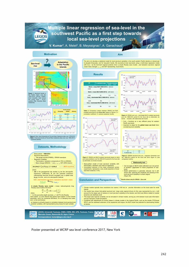
242

Multiple linear regression of sea-level in the southwest Pacific as a first step towards

local sea-level projections V. Kumar1, A. Melet2, B. Meyssignac1, A. Ganachaud1

Motivation

Adaptation in the Pacific

islands Sea-level

rise

Aim

The aim is to develop a statistical model for local sea-level variability in the south western Pacific islands on interannual-to-decadal timescales, and for long-term trends. We reconstruct local sea-levels using a multi-linear regression model, with Curlz τ as the dominant regional predictor (from a simple Rossby wave model) , and halosteric sea-level, regional ocean mass changes, τx, τy, and SST representing local drivers.

Datasets, Methodology

Results

sla (site,t) = ∑I αi Pi (xi yi, t ) + ε(site,t) - - - - - (MLR equation)

SSH = thermosteric sea level + halosteric sea level + mass

Curlz τ Rossby wave propagation

-  Study period – 1988-2014 -  Sea-level observations:

•  Tide gauge records (PSMSL), ORAS4 reanalysis -  Regressor variables:

•  Thermosteric, halosteric components (≤ 700 m) (ORAS4) •  Mass change (GRACE) • curlz τ, τx, τy, SST (ERA-Interim)

Conclusion and Perspectives

•  Climate models typically have resolutions too coarse (~100 km) to provide information on the local scale for small islands

•  Our results have shown that global sea-level and large scale regional drivers (in this case represented by curlz τ) still account for the larger part of variance in local sea-level variability at the islands, and that local effects related to coastal dynamics are relatively small

•  This large-scale regional variability can be simulated in climate models, serving as a link between local scale information and low resolution model simulations.

•  Combined with adjustments for known biases in climate models in the tropical Pacific, such as the double ITCZ/zonal SPCZ, and the westward extension of the equatorial cold tongue, the MLR model has potential for downscaling studies at islands.

Figure 1: Sea-level trends in the Pacific region over the 1993-2014 period (GMSL trend included). Inset shows the study sites – Suva, Lautoka (Fiji), Nouméa (New Caledonia)

where: •  site is the geographical site studied, αi are the site-specific

regression coefficients, Pi are the potential predictors (representing sea-level drivers) averaged over a spatial area (xi,yi), t is time , and ε is a site-specific residual.

A simple Rossby wave model : Linear, reduced-gravity long Rossby wave model of the form:

•  h is the pycnocline depth anomaly, cr = -βc2/f2 is the Rossby

wave speed (c is the internal long gravity wave speed, f is the Coriolis parameter, and β its meridional derivative, R is a damping time scale, and τ is the wind stress)

(a)

(b)

(a)

(b)

1LEGOS, Université Toulouse, CNES, CNRS, IRD, UPS, Toulouse, France

Correspondence: [email protected]

2Mercator Ocean, Ramonville St. Agne, France

dhdt+ cr dh

dx+ Rh = −curl τ

f ρ"

#$

%

&'


SLA

(mm

)

-200

-100

0

100

200Noumea tgORAS4altimetry


SLA

(mm

)

-200

-100

0

100

200Lautoka tgORAS4altimetry


SLA

(mm

)

-200

-100

0

100

200 Suva tgORAS4altimetry

Site

Trends (mm/yr) Tide-gauge ORAS4 Altimetry

1993-2014 (a) 8.2 5.7 5.8 (b) 5.1 5.5 5.2 (c) 2.4 4.1 4.0

(a)

(b) (c)

Figure 2: Sea -level timeseries at Fiji and New Caledonia sites over 1979-2012 Table 1: Sea-level trends at Fiji and New Caledonia sites over over 1993-2014 (common period)

Table 2: Comparison metrics between ORAS4 and MLR modeled sea-levels for the Suva site, based on Figures 3, 4 (correlation coefficient, % variance explained, trends)

R2 % variance exp. Trends (mm/yr)

Steric + mass MLR (2003-2014) - detrend0.94 89 -- --

Steric + mass MLR (2003-2014) - with trend

0.95 91 7.9 7.5Curlz τ dominated MLR (1988-2014) - detrend

0.92 85 -- --Curlz τ dominated MLR (1988-2014) - with trend

0.92 86 1.6 1.8

where

* Results shown only for ORAS4 – Suva site

•  Near-perfect model of local sea-level variability with thermosteric, halosteric and mass as regressors

•  Inconsistent behavior of the mass component across experiments, represents a very small proportion of local sea-level variance (< 5%)

Figure 3: ORAS4 and MLR modeled sea-levels based on steric and mass predictors over the 2003-2014 period for the Suva site (a) detrended, (b) trends included


SLA

(mm

)

-150

-100

-50

0

50

100

150

Suva ORAS4MLR total


SLA

(mm

)

-150

-100

-50

0

50

100

150

Suva ORA-S4mlr totalmlr 1st halfmlr predicted 2nd halfmlr 2nd halfmlr predicted 1st half

•  Curlz τ functions as a very efficient proxy for western Pacific sea-levels

•  Important to adjust for the global mean sea level when considering local variability


SLA

(mm

)

-100

-50

0

50


Figure 4: ORAS4 and curlz τ dominated MLR modeled sea-levels over the 1988-2014 period for the Suva site a) detrended, (b) trends included, with stationarity test results


SLA

(mm

)

-150

-100

-50

0

50

100


•  Can we apply an MLR model calibrated over one period to another? (application to future projections of sea-level)

•  Model performance is generally reduced, but it still shows skill, capturing the amplitude and phasing of the local sea level variability to certain degree

(Figure 4b)

Stationarity test

ORAS4 Model

Figure 5: ORAS4 sea-level and curlz τ regressor timeseries over the 1988-2014 period for the Suva site (from Figure 4), plus comparison metrics

(a)

(b)

(b)

(a)

► Analysis is primarily based on correlation between local sea-level and predictor variables, with representative proxy boxes for each variable


SLA

(mm

)

-150

-100

-50

0

50

100

150

Suva ORAS4WS curl

R2 0.85 % variance exp. 73

Poster presented at WCRP sea level conference 2017, New York

Statistical downscaling of island sea levels in the southwest ...

Documents

Transcript of Statistical downscaling of island sea levels in the southwest ...