Hedging: Scaling and the Investor Horizon*

John Cotter and Jim Hanly

Keywords: Hedging Effectiveness; Scaling; Volatility Modelling, Forecasting.

JEL classification: G10, G12, G15.

August 2009 John Cotter, Director of Centre for Financial Markets, School of Business University College Dublin, Blackrock, Co. Dublin, Ireland, Tel 353 1 716 8900, e-mail john.cotter@ucd.ie. Jim Hanly, School of Accounting and Finance, Dublin Institute of Technology, Dublin 2, Ireland. tel 353 1 402 3180, e-mail james.hanly@dit.ie.

*The authors would like to thank participants at a University College Dublin seminar for their comments on an earlier draft. Part of this study was carried out while Cotter was visiting the UCLA Anderson School of Management and is thankful for their hospitality. Cotter’s contribution to the study has been supported by a University College Dublin School of Business research grant. The authors thank an anonymous referee for helpful comments but the usual caveat applies.

1

Hedging: Scaling and the Investor Horizon

Abstract

This paper examines the volatility and covariance dynamics of cash and futures

contracts that underlie the Optimal Hedge Ratio (OHR) across different hedging time

horizons. We examine whether hedge ratios calculated over a short term hedging

horizon can be scaled and successfully applied to longer term horizons. We also test

the equivalence of scaled hedge ratios with those calculated directly from lower

frequency data and compare them in terms of hedging effectiveness. Our findings show

that the volatility and covariance dynamics may differ considerably depending on the

hedging horizon and this gives rise to significant differences between short term and

longer term hedges. Despite this, scaling provides good hedging outcomes in terms of

risk reduction which are comparable to those based on direct estimation.

2

Hedging: Scaling and the Investor Horizon

I Introduction

Much of the large body of work on hedging has focused on short time horizons such as

a 1-day frequency1. This ignores the fact that the OHR is dependent on the time horizon

and that a hedge calculated from data at one frequency may not provide good risk

reduction outcomes over lower frequencies. Also, there is no definitive answer to the

question of what constitutes the relevant horizon for risk management since investors

have differing investment horizons. Research suggests a variety of horizons ranging

from 1-day for traders, to 1-month or even 12 months for investors and corporate risk

management respectively.2 However, the estimation of hedge strategies over longer

term time horizons such as weekly or monthly can be problematic. The key problem is

that for lower frequency data, fewer observations are available on which to base the

estimation (Hwang and Valls Pereira, 2006). For example, an estimation period of 5-

years of daily data will yield around 1300 observations; however, this number drops to

around 260 for the weekly frequency and just 60 if data at the monthly frequency are

used. Using a longer estimation period such as 20 years may not yield better estimates

since OHR’s are time varying (Lien and Tse, 2002). This means that using a very long

estimation period may be suboptimal, as some of the data may not be relevant given

their temporal distance.3 Also, time varying hedge strategies such as those calculated

using GARCH models, require large numbers of observations if the model is to meet the

1 See Lien and Tse (2002), for a review of the development of the literature on optimal hedging.

2 See Locke (1999), Smithson and Minton (1996), for evidence on the variety of time horizons that are relevant to

investors. 3 See for example Merton (1980) who finds that better volatility estimates are to be had from using a large number

of high frequency data rather than a small number of low frequency data over a longer time period.

3

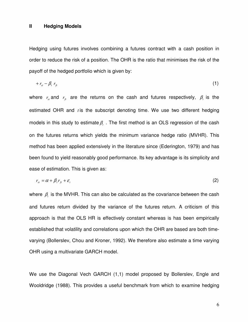
non-negativity constraints which are a typical feature of those models4. The estimation

and statistical problems related to low sample size, have led to the adoption by risk

managers, of models that estimate volatility at one frequency (say daily) and then scale

the volatility estimate to obtain low frequency volatilities (say monthly). A number of

scaling laws have been applied in financial applications. Initially these were based on

Gaussian distributions and random walks which allowed scaled sums of Gaussians to

follow the same distribution. Further work by Mandelbrot (1963) proved that daily prices

were not from a Gaussian distribution and a number of papers, including Dacarogna,

Muller, Pictet and De Vries (1998) provided evidence of scaling and power laws in many

financial time series5. Scaling has been used in many applications in financial

economics, most notably in the Black-Scholes-Merton option pricing framework and in

risk management and banking regulation, where scaling is based on the Square-Root-

of-Time (SQRT) rule 6. For example, a typical daily volatility estimate for equity index

data using the standard deviation would be about 1.3%. Applying the SQRT rule to

obtain a monthly estimate would yield a volatility of 5.8%, or an annual estimate of

about 21%.

While scaling has been extensively applied in the literature on volatility and high

frequency finance, little work has been done on scaling and hedging. However, a

number of papers have examined hedging for different time horizons (see Malliaris and

Urrutia (1991), Geppert (1995), Chen, Lee and Shrestha (2004) and In and Kim (2006)),

and the findings show that as the hedging horizon increases, both the OHR and the in-

sample hedging effectiveness increase. There are contrasting findings out-of-sample

4 See Hwang and Valls Pereira (2006) for a discussion.

5 For an extensive discussion on scaling laws in finance see Brock (1999).

6 The Basel agreements on banking supervision require that daily volatility estimates be scaled using the SQRT rule.

4

with some papers reporting decreased effectiveness at longer time horizons (Malliaris

and Urrutia, 1991). However, most papers report a positive relationship between hedge

horizon and hedging effectiveness (Chen et al, 2004, Lien and Shrestha, 2007). A

variety of methods have been used to calculate hedges over longer time horizons.

These include the use of models based on the underlying data generating process and

more recently the use of wavelet analysis7.

In this paper we calculate a hedge ratio at a relatively high frequency using a 1-day

(daily) time horizon. We then apply this hedge ratio by scaling it up to both 5-day

(weekly) and 20-day (monthly) frequencies. We compare the scaled hedge ratios with

OHR’s that are estimated by matching the frequency of the data to the hedging

horizon8. We also re-examine the issue of hedging effectiveness across different time

horizons using the performance evaluation criteria of Value at Risk (VaR) and

Conditional Value at Risk (CVaR). To our knowledge, these criteria have not been

applied in the literature on hedging to evaluate hedges over different time horizons.

Indeed the findings on the relationship between hedging effectiveness and time horizon

are based on a single evaluation criterion which is variance. By applying additional

performance evaluation criteria, we will provide additional evidence on the issue of

hedging effectiveness across different time horizons.

A further contribution of this paper is an analysis of the levels of persistence in volatility

for different hedging horizons. Drost and Nijman (1993), Diebold et al (1998), and

Christofferson, Diebold and Schuermann (1998), all address the issue of how the

7 For example, Geppart (1995) use a Data Generating Process to generate returns at different time horizons while In

and Kim (2006) apply wavelets to decompose the variance and covariance over different time scales. 8OHR’s estimated in this way are hereafter referred to as actual hedges or equivalently ‘direct estimation’.

5

accuracy of volatility forecasts change with the time horizon. The findings of these

papers show that forecastability will decrease as we move from short to long time

horizons. We investigate the implications of this finding for optimal hedging by

examining the temporal aggregation properties of GARCH models that have been

successfully used to estimate time varying OHR‘s. This allows us to draw a link

between the literature on volatility persistence and hedging performance.

Our findings show that actual hedge strategies statistically outperform scaled hedge

strategies; however the differences are only marginal when viewed from an economic

perspective. Furthermore, we find that scaled hedges are effective in that they provide

acceptable reductions in risk as measured by Variance, VaR and CVaR. We also

provide evidence that ex-post hedging effectiveness increases as we move from high to

low frequency hedging. Finally, we show that lower levels of volatility persistence, does

not materially affect the ex-post hedging effectiveness at lower frequencies implying that

GARCH models can still provide good forecast outcomes over longer hedging horizons.

The remainder of the paper proceeds as follows. In section II we outline the hedging

models. In Section III we detail the scaling approach. In Section IV we describe the

metrics for measuring hedging effectiveness. Section V describes the data followed by

our empirical findings in Section VI. Finally, Section VII summarises and concludes.

6

II Hedging Models

Hedging using futures involves combining a futures contract with a cash position in

order to reduce the risk of a position. The OHR is the ratio that minimises the risk of the

payoff of the hedged portfolio which is given by:

fttst rr β−+ (1)

where str and ftr are the returns on the cash and futures respectively,

tβ is the

estimated OHR and t is the subscript denoting time. We use two different hedging

models in this study to estimatetβ . The first method is an OLS regression of the cash

on the futures returns which yields the minimum variance hedge ratio (MVHR). This

method has been applied extensively in the literature since (Ederington, 1979) and has

been found to yield reasonably good performance. Its key advantage is its simplicity and

ease of estimation. This is given as:

tfttst rr εβα ++= (2)

where tβ is the MVHR. This can also be calculated as the covariance between the cash

and futures return divided by the variance of the futures return. A criticism of this

approach is that the OLS HR is effectively constant whereas is has been empirically

established that volatility and correlations upon which the OHR are based are both time-

varying (Bollerslev, Chou and Kroner, 1992). We therefore also estimate a time varying

OHR using a multivariate GARCH model.

We use the Diagonal Vech GARCH (1,1) model proposed by Bollerslev, Engle and

Wooldridge (1988). This provides a useful benchmark from which to examine hedging

7

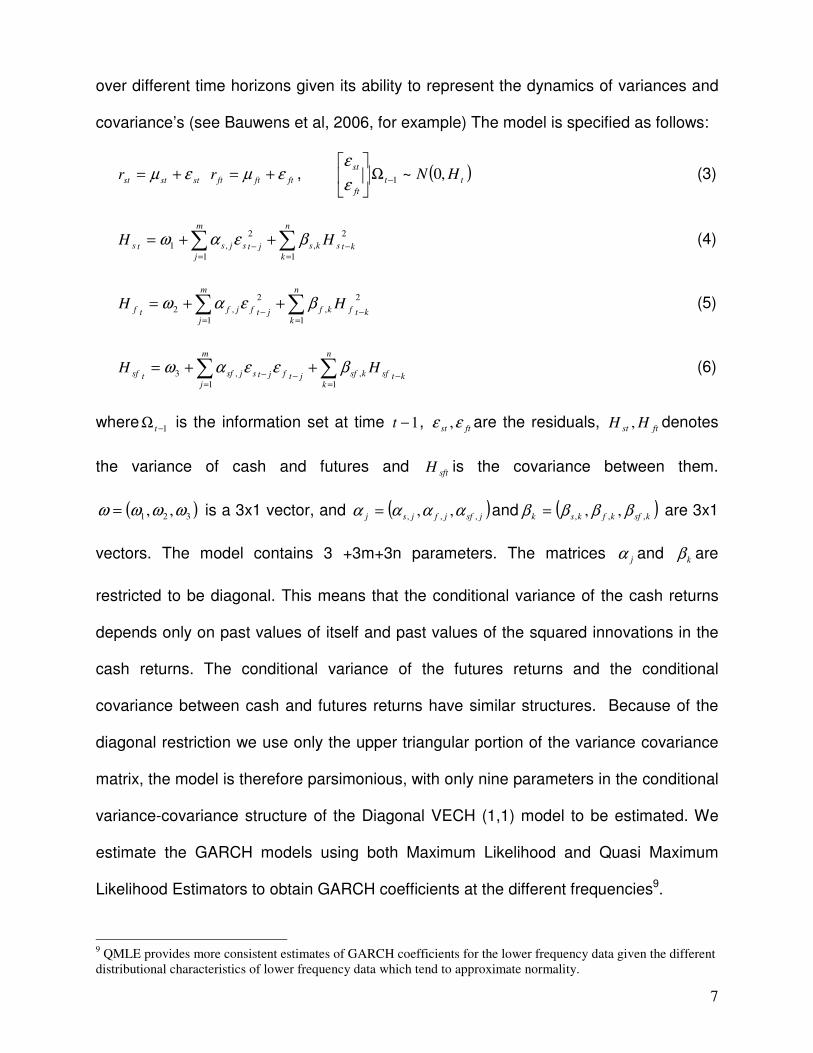
over different time horizons given its ability to represent the dynamics of variances and

covariance’s (see Bauwens et al, 2006, for example) The model is specified as follows:

stststr εµ += ftftftr εµ += , ( )tt

ft

stHN ,0~1−Ω

ε

ε (3)

∑∑=

−=

−++=

n

k

ktsks

m

j

jtsjsts HH1

2

,

1

2

,1 βεαω (4)

∑∑=

−=

−++=

n

kktfkf

m

jjtfjftf HH

1

2

,

1

2

,2 βεαω (5)

∑∑=

−−=

−++=

n

kktsfksfjtf

m

j

jtsjsftsf HH1

,

1

,3 βεεαω (6)

where1−Ω t is the information set at time 1−t , ftst εε , are the residuals, ftst HH , denotes

the variance of cash and futures and sftH is the covariance between them.

( )321 ,, ωωωω = is a 3x1 vector, and ( )jsfjfjsj ,,, ,, αααα = and ( )

ksfkfksk ,,, ,, ββββ = are 3x1

vectors. The model contains 3 +3m+3n parameters. The matrices jα and kβ are

restricted to be diagonal. This means that the conditional variance of the cash returns

depends only on past values of itself and past values of the squared innovations in the

cash returns. The conditional variance of the futures returns and the conditional

covariance between cash and futures returns have similar structures. Because of the

diagonal restriction we use only the upper triangular portion of the variance covariance

matrix, the model is therefore parsimonious, with only nine parameters in the conditional

variance-covariance structure of the Diagonal VECH (1,1) model to be estimated. We

estimate the GARCH models using both Maximum Likelihood and Quasi Maximum

Likelihood Estimators to obtain GARCH coefficients at the different frequencies9.

9 QMLE provides more consistent estimates of GARCH coefficients for the lower frequency data given the different

distributional characteristics of lower frequency data which tend to approximate normality.

8

III Scaling

The determination of the OHR requires an estimate of the variance of the futures return

at whatever frequency is being examined, together with an estimate of the covariance or

correlation between the cash and futures return. The problem of estimating volatility

over longer term time horizons has been examined in some detail in the risk

management literature. Risk managers have good high frequency data but require

reliable estimates of volatility at low frequencies corresponding to the respective holding

periods of investors. An alternative approach is to estimate volatility using high

frequency data and then scale it to obtain low frequency estimates. The most popular

method of scaling volatilities is based upon the SQRT rule. The theoretical justification

and background for the SQRT rule is as follows: ConsidertS , the log price of an asset at

time t , where the changes in the log price are independent and identically distributed

(i.i.d.). Then the price at time t can be expressed as

ttt SS ε+= −1 ( )2

, ,0~ σε it (7a)

and the 1-day return, is

tttt SSr ε=−= −1 (7b)

with variance 2σ . Aggregating h-day returns results in

t

h

n

htnthttt SSr εεε ++==−= ∑−

=

+−−−

1

0

1 ... (7c)

with variance 2σh and standard deviation σh , which implies the square-root-of-time

rule. This rule can be considered a special case of the more general empirical scaling

law discussed by Dacarogna et al (2001), which gives a direct relation between time

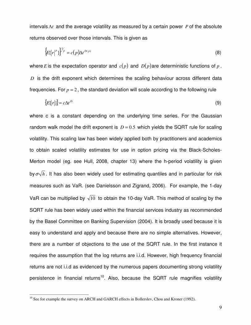
9

intervals tΛ and the average volatility as measured by a certain power P of the absolute

returns observed over those intervals. This is given as

( ) )(1

][ pDpptpcrE ∆= (8)

where E is the expectation operator and ( )pc and ( )pD are deterministic functions of p .

D is the drift exponent which determines the scaling behaviour across different data

frequencies. For 2=p , the standard deviation will scale according to the following rule

DtcrE ∆=][ (9)

where c is a constant depending on the underlying time series. For the Gaussian

random walk model the drift exponent is 5.0=D which yields the SQRT rule for scaling

volatility. This scaling law has been widely applied both by practitioners and academics

to obtain scaled volatility estimates for use in option pricing via the Black-Scholes-

Merton model (eg. see Hull, 2008, chapter 13) where the h-period volatility is given

by hσ . It has also been widely used for estimating quantiles and in particular for risk

measures such as VaR. (see Danielsson and Zigrand, 2006). For example, the 1-day

VaR can be multiplied by 10 to obtain the 10-day VaR. This method of scaling by the

SQRT rule has been widely used within the financial services industry as recommended

by the Basel Committee on Banking Supervision (2004). It is broadly used because it is

easy to understand and apply and because there are no simple alternatives. However,

there are a number of objections to the use of the SQRT rule. In the first instance it

requires the assumption that the log returns are i.i.d. However, high frequency financial

returns are not i.i.d as evidenced by the numerous papers documenting strong volatility

persistence in financial returns10. Also, because the SQRT rule magnifies volatility

10

See for example the survey on ARCH and GARCH effects in Bollerslev, Chou and Kroner (1992).

10

fluctuations when they should be damped, it tends to produce overestimates of long-

horizon volatility (see Diebold et al, 1998 for a discussion).

Despite these issues, the SQRT method has been widely adopted in risk management

and banking as a means of obtaining low frequency volatilities. Dowd and Oliver (2006)

provide limited support for the use of the SQRT rule. They suggest that the key to using

the SQRT rule is to apply it to the unconditional volatility as opposed to the most recent

estimate11. Furthermore, Anderson et al (2001) report the means of the popular

measure realized variance estimators grow linearly with time, which would be consistent

with the SQRT rule. Dacarogna et al (2001) find that this scaling law is appropriate for a

wide range of financial data and for time intervals ranging from 10 minute to more than

a year. They also estimate scaling exponents for foreign exchange data and find values

of D very close to 0.5 for USD/GBP and other exchange rates. Additional support for

the SQRT rule is put forward by Brummelhuis and Kaufman (2007) who apply it for

scaling quantiles and conclude that it provides reasonable estimates for risk

management purposes. Therefore, the use of the SQRT rule should provide a good

approximation in terms of converting volatility from one frequency to another frequency

even where the distribution is not strictly normal.

An alternative to scaling volatility by time is the use of formal model based aggregation

as proposed in Drost and Nijman (1993) (henceforth DN), who study the temporal

aggregation of GARCH processes. They propose the following approach: Suppose we

11

This finding is based on a simulations based approach which indicate that if the daily volatility used as the basis of

extrapolation is greater than the unconditional volatility it results in the SQRT rule overestimating the GARCH or

‘true’ volatility and vice versa. Therefore they conclude that the SQRT rule is appropriate only where the daily

volatility to be used as the basis for extrapolation is equal to unconditional volatility.

11

begin with have a sample path of one-day returns T

ttR1)1( =which follow a weak GARCH

(1, 1) process as follows:

)1,0(~

2

1

2

1

2

NID

y

R

t

ttt

ttt

ε

βσαωσ

εσ

−− ++=

=

(10)

for Tt ,...,1= where 2

tσ is the variance and βαω ,, are the estimated parameters on the

GARCH model. The following stationarity and regularity conditions are

imposed, ∞<< ω0 , and 1,0,0 <+≥≥ βαβα .Then DN show that, under regularity

conditions, the corresponding sample path of h-day returns, hT

tthR/

1)( =also follows a

GARCH (1, 1) process with

2

1)()(

2

1)()()(

2

)( −− ++= thhthhhth y σβαωσ (11)

where

( )( )αβ

αβωω

+−

+−=

1

1)(

h

h h (12)

( ) ,)()( h

h

h βαβα −+= (13)

and 1)( <hβ is the solution of the quadratic equation,

( )( )( )

,211 22

)(

)(

ba

bah

h

h

h

−++

−+=

+ αβ

αβ

β

β (14)

where

( ) ( ) ( ) ( )( ) ( )( )

( ) ( )( ) ( )( )( )2

2

222

1

14

11

211121

αβ

αββαααβαβ

αβκ

βαβαββ

+−

+−+++−−+

+−−

−−−−−+−=

hhh

hhha

(15)

( )( ) ( )( )

,1

12

2

αβ

αβαββαα

+−

+−+−=

h

b (16)

12

and κ is the kurtosis of ty . This approach allows us to fit a GARCH model at one

frequency (eg. 1-day) and the model coefficients obtained αω, and β can then be

substituted into the DN equations to obtain scaled coefficients at another frequency

(E.g. 5-day). Also this formula can be used to convert 1-day covariance to h-day

covariance if we substitute the covariance parameters from a multivariate GARCH

model12. This approach is useful at generating parameter values at long time horizons

from short time horizons. From the formulas for hα and

hβ ,

0,0 →→ hh βα as ∞→h .This means that asymptotically the volatility becomes constant,

and therefore the weak GARCH(1,1) process behaves in the limit like a random walk.

This implies that conditional forecasts will have poor performance over long periods as

predictability decreases. A number of papers have examined the usefulness of the DN

approach. Diebold et al (1998) show that if the short horizon return model is correctly

specified as a GARCH (1, 1) process, then the DN approach can be used for the correct

conversion of 1-day to h-day volatility. Kaufman and Patie (2003) use the DN formula in

a simulation based approach and conclude that it provides good parameter estimates

based on daily data scaled to horizons of up to 1-month. A shortcoming of the approach

is that it assumes an exact fit for the model whereas in general it is an approximation13.

In this paper we provide further evidence on the applicability of the DN approach. We

measure volatility persistence by fitting a GARCH (1, 1) model directly from the data at

the relevant time horizon. We then use the DN formula to obtain scaled parameters

from the 1-day data for both 5-day and 20-day horizons. This allows us to compare the

12

Therefore the DN approach can be used to scale hedge ratios which are composed of both variance and covariance

components. 13

See Christoffersen, Diebold, & Schuermann (1998) for a detailed discussion of the conditions under which

temporal aggregation formulae may by used.

13

volatility parameters estimated directly from the data with those obtained by scaling.

This also allows us to examine the persistence of volatility across different time horizons

and in so doing, to draw inferences about the relative forecasting ability of GARCH

models across different time horizons. Our ex-ante expectation is that volatility

persistence will decrease with the hedging horizon, and that this may affect the ex-post

forecasting performance of hedges at lower frequencies.

The determinants of the optimal hedge are the covariance between the cash and

futures return and the variance of the futures return. Similar to the variance, the

covariance can also be scaled by time under the i.i.d and normality assumptions.

However, whatever the scaling method applied, the composition of the OHR effectively

means that both the numerator and the denominator are scaled by the same factor. This

means that when we scale the OHR, we are effectively applying a hedge ratio

calculated at one frequency to hedges applied at a different frequency. We now turn to

methods employed to measure the effectiveness of our hedges.

IV Hedging Effectiveness

We compare hedging effectiveness using the percentage reduction in the variance of

the cash (unhedged) position as compared to the variance of the hedged portfolio. This

is given as:

% Variance Reduction

−=

rtfolioUnhedgedPo

folioHedgedPort

VARIANCE

VARIANCE1 (17)

This measure of effectiveness has been used in the literature on hedging over different

time horizons, however hedgers may seek to minimise some measure of risk other than

14

the variance. For this reason, we use two additional hedging effectiveness metrics that

will allow us to compare the hedging performance of scaled hedges with hedges

calculated with data matched to the time horizon. While these metrics have been

applied before to the hedging problem (see Cotter and Hanly, 2006), they have not

been used to examine the relationship between time horizon and hedging effectiveness.

The second hedging effectiveness metric is VaR. For a portfolio this is the loss level

over a certain period that will not be exceeded with a specified probability. The VaR at

the confidence levelα is

αα qVaR = (18)

where αq is the relevant quantile of the loss distribution. The performance metric

employed is the percentage reduction in the VaR of the hedged as compared with the

unhedged position.

−=

rtfolioUnhedgedPo

folioHedgedPort

VaR

VaRHE

%1

%1

2 1 (19)

The third hedging effectiveness metric is the CVaR14 which is the average of the worst

( ) %1001 α− of losses.

In effect this means taking the average of quantiles in which tail quantiles are equally

weighted and non-tail quantiles have zero weight.15 The performance metric we use to

evaluate hedging effectiveness is the percentage reduction in CVaR as compared with

a no hedge position.

14

This is also called the Expected Shortfall. 15

For more detail on the properties of the CVaR see Cotter and Dowd (2006)

15

−=

rtfolioUnhedgedPo

folioHedgedPort

CVaR

CVaRHE

%1

%1

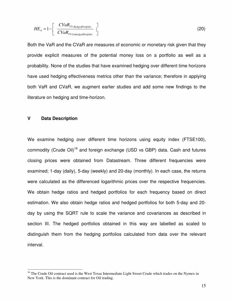
4 1 (20)

Both the VaR and the CVaR are measures of economic or monetary risk given that they

provide explicit measures of the potential money loss on a portfolio as well as a

probability. None of the studies that have examined hedging over different time horizons

have used hedging effectiveness metrics other than the variance; therefore in applying

both VaR and CVaR, we augment earlier studies and add some new findings to the

literature on hedging and time-horizon.

V Data Description

We examine hedging over different time horizons using equity index (FTSE100),

commodity (Crude Oil)16 and foreign exchange (USD vs GBP) data. Cash and futures

closing prices were obtained from Datastream. Three different frequencies were

examined; 1-day (daily), 5-day (weekly) and 20-day (monthly). In each case, the returns

were calculated as the differenced logarithmic prices over the respective frequencies.

We obtain hedge ratios and hedged portfolios for each frequency based on direct

estimation. We also obtain hedge ratios and hedged portfolios for both 5-day and 20-

day by using the SQRT rule to scale the variance and covariances as described in

section III. The hedged portfolios obtained in this way are labelled as scaled to

distinguish them from the hedging portfolios calculated from data over the relevant

interval.

16

The Crude Oil contract used is the West Texas Intermediate Light Sweet Crude which trades on the Nymex in

New York. This is the dominant contract for Oil trading.

16

Because we are examining low frequency data, we required a dataset that would be

large enough to allow us to be able to fit the time varying GARCH model17 and to carry

out estimation with a reasonable degree of statistical accuracy. The full sample runs

from March 29, 1993 through March 6, 2008. The estimation sample runs from March

29, 1993 through March 17, 2003 or about 10 years of data. This provides us with 2601

1-day, 521 5-day and 131 20-day observations. The remaining observations were used

as a hold out sample.

[INSERT TABLE I HERE]

Descriptive statistics for the data are displayed in Table I. The following properties of the

data are worth noting. As we move from the 1-day frequency to lower frequencies, the

mean and volatility, as measured by the standard deviation increase. One of the more

important results from a hedging perspective is that the correlation between cash and

futures increases as we move from high to low frequency18. Also, correlations at the 1-

day frequency are very different for the different assets. For example, the correlation is

0.970 for the FTSE100 but just 0.876 for Oil and 0.816 for USD/GBP. When we look at

the 20-day frequency, however, there is little difference between the correlations for the

different assets which are 0.992, 0.993 and 0.989 for FTSE100, Oil and USD/GBP

respectively. This means hedging effectiveness should increase as we hedge longer

time horizons, but also that for shorter time horizons there may be significant

17

Hwang and Valls Pereira (2006) in an examination of the small sample properties of GARCH models report that

very small numbers of observations can cause unreliable parameter estimates. Our dataset is large enough to

generate reasonable estimates from the GARCH model. 18

This finding was discussed at length in Geppert (1995) who pointed out that given a cointegrated relationship

between spot and futures prices which is made up of both permanent and transitory components, over longer

horizons the permanent component ties the futures and spot together while the effect of the transitory component

becomes negligible.

17

differences between the different assets in terms of hedging effectiveness. For this

reason, the hedging model choice may be more important at the 1-day frequency.

The distribution of the data is significantly non-normal at the 1-day interval whereas at

lower frequencies the data are more symmetric. For both Oil and USD/GBP, the data

can be characterised as Gaussian at the 20-day frequency, as we fail to reject the

hypothesis of normality at conventional significance levels. This implies that scaling

using the SQRT rule may be more appropriate using lower frequency data19. We find

significant ARCH effects at the 1% level at the 1-day frequency for each of the assets

with the exception of USD/GBP which is significant at the 5% level, however, these

diminish at lower frequencies. We can also observe a difference between the

characteristics of the FTSE100 as compared with both the Oil and USD/GBP data. For

example the FTSE100 exhibits significant ARCH effects across each hedging horizon

(p-values of 0.01 or lower) whereas the Oil and USD/GBP data which have significant

ARCH effects at the 1-day frequency only, have insignificant ARCH effects at the 5-day

and 20-day frequencies. This finding agrees with the well known result from the

literature that volatility persistence decreases as we move from high to low frequency

data (see, for example, Poon and Granger, 2003). The implication is that GARCH

models will generate better forecasts at shorter time horizons. However, in this paper

we are estimating the ex-post hedge ratio using 1-step-ahead forecasts so it remains to

be seen whether the lower volatility persistence at lower frequency will affect the

efficiency of the hedges20. Stationarity is tested using both the Phillips Peron and

19

This finding means that scaling may be more applicable from say 20-Day to 1-Year than from 1-Day to 20-Day

however the problem of having enough observations at even the 20-Day interval remains. 20

Christofferson and Diebold (2000) find that volatility forecasts are unreliable beyond 10 days. However they used

daily data which means in effect that volatility is forecastable up to 10-steps. In this study although we are

generating a forecasts of up to 20-days ahead for the 20-Day horizon, it is based on a 1-step forecast.

18

Kwiatkowski, Phillips, Schmidt and Shin (KPSS) tests21. The results of both tests

indicate that the log returns series is stationary irrespective of the sampling frequency.

This indicates that the OLS estimates should be reliable across each of the time

horizons.

VI Empirical Findings

[INSERT TABLE II HERE]

Table II reports the GARCH parameters using direct estimation at the 1-day, 5-day and

20-day frequencies together with the scaled parameters estimated from the 1-day data

using the Drost Nijman approach. Examining first the results of direct estimation, as we

move from high frequency to low frequency the level of persistence in volatility is

significantly reduced. This is most pronounced for the Oil and USD/GBP data. For

example, as we move from 1-day to 5-day, volatility persistence22 for the FTSE drops

just over 1% from 0.986 to 0.975 for cash23. In the case of Oil, persistence decreases by

about 16% from 0.696 to 0.528 while for USD/GBP the drop is even more pronounced

going from 0.853 to 0.554. When we examine the results for the 20-day frequency,

persistence is still relatively high for the FTSE at 0.875, whereas for both Oil and

USD/GBP it is in the region of just 0.10. These findings are supportive of previous work

such as Christofferson Diebold and Schuermann (1998) that have found that volatility

persistence decreases as the time horizon increases, or alternatively as we move from

high frequency to low frequency data. The implications of this relate to the forecasting

ability of the GARCH models at lower frequency, where we may see a performance

21

For brevity we have only included the results from the KPSS test in Table I. 22

As measured by the sum of the A or ARCH coefficient and the B or GARCH coefficient. 23

For brevity we base the parameter comparisons on the cash asset unless otherwise stated.

19

differential in the ex-post hedging effectiveness of the hedges for the different assets at

different frequencies.

We also report the scaled parameters obtained using the DN approach based on inputs

from the GARCH model at the 1-day frequency. Comparing first the scaled parameters

for the FTSE, they are broadly in line with the parameters obtained from direct

estimation at the 5-day frequency but when we move to the 20-day frequency larger

differences emerge. For example, the scaled parameters at the 5-day frequency are

lower by about 2% – 3% as compared with the 5-day actual. When we move to the 20-

day frequency, however, there are significant differences. For example, persistence as

measured using the scaled coefficients at 0.761 is significantly lower than the actual

estimate of 0.875 would suggest. For both Oil and USD/GBP, the scaled parameters

are significantly different from the actual parameters at both the 5-day and 20-day

frequencies. For Oil, actual volatility persistence at the 5-day frequency is 0.528 and

0.099 at the 20-day frequency. This compares with scaled persistence of 0.163 and just

0.0007 for the 5-day and 20-day frequencies respectively. Similarly, the actual

coefficients for the USD/GBP data are very different from those obtained using the DN

approach. These findings indicate that the DN approach may provide a reasonable

approximation for the volatility data generating process for equity returns using a scaling

factor in the region of 5, from 1-day to 5-day. This finding agrees with Kaufmann and

Patie (2003) who found that the DN approach provided reasonable estimates of

coefficients when scaling from 1-day frequency up to 1-week. However for other assets

such as Oil or foreign exchange rates, the coefficient estimates obtained by scaling do

not approximate those obtained by direct estimation.

[INSERT TABLE III HERE]

20

[INSERT FIGURES 1A, 1B AND 1C HERE]

The estimated optimal hedges are presented in Figures 1a, 1b and 1c together with

their associated statistics in Table III. All hedges are less than 1 with the exception of

the USD/GBP at the 20-day frequency24. For the FTSE and USD/GBP, the OHR’s

increase in line with the time horizon and tend to approach the Naïve hedge ratio which

is 1. For example, the mean OHR for the FTSE goes from 0.875 to 0.934 to 0.957 as

we move from the 1-day frequency to the 5-day and 20-day frequencies respectively.

This means that the investor would sell a larger number of futures contracts to achieve

the optimal hedge as the frequency of the hedge increases. This would have

implications on the cost of the hedging strategy. For example, it would mean that

hedging a single 20-day period would be more expensive than a single 1-day period.

For Oil, the OHR’s increase as we move from the 1-day to the 5-day horizon from 0.929

to 0.992. However, while there is then a slight decrease with the 20-day OHR at 0.987.

the results are broadly similar to those for the FTSE and USD/GBP. Also the mean

OHR’s for the different time horizons are significantly different based on standard t-tests

at the 1% level. These findings reflect the fact that the correlation between cash and

futures increases as we move from high frequency to low frequency data.

The OLS hedges also tend to increase with the hedging horizon with the exception of

Oil for the 20-day frequency. These results are consistent with the literature (see, for

example, Chen Lee and Shrestha, 2004) in that for longer investment horizons, the

optimal hedge ratio converges towards the Naïve hedge ratio. In terms of dispersion of

the OHR’s, there are also large differences in the standard deviations of the OHR’s at

24

A hedge ratio in excess of 1 implies that an investor hold a naked short position in futures which in some cases

would be necessary in order to achieve the minimum variance portfolio.

21

the different time horizons. This is most pronounced for the Oil hedges. For example,

the standard deviation of the 1-day time varying OHR is 0.127 but this drops to 0.053 for

the 5-day OHR’s and to just 0.008 for the 20-day hedge. This can be confirmed with a

quick glance at figure 1b. This finding highlights the fact that at we move from high to

low frequency hedges, the gap between the time-varying and the constant hedges

narrows.

We now turn to the hedging effectiveness of the hedge strategies and compare the

effectiveness of hedges calculated directly using data at the relevant hedging horizon

with the hedges based on scaling. Table IV presents the hedging effectiveness metrics

for both OLS and GARCH models across hedging horizons. Hedging models are

compared in terms of the percentage reduction in a given risk measure as compared

with a no-hedge position. The effect of hedging horizon on hedging effectiveness is

apparent in that in-sample hedging effectiveness increases with the hedging horizon.

For example, using the variance as the performance criterion, both the OLS and

GARCH hedges for USD/GBP yield around a 67% reduction in risk at the 1-day horizon.

This increases to around 90% at the 5-day horizon and around 98% at the 20-day

horizon. Both FTSE and Oil exhibit similar results25.

The differences between the hedging performances at the different time horizons are

also statistically significant at the 1% level i.e. the 5-day performance is statistically

significantly better than the 1-day performance, similarly the 20-day is significantly

25

Results are rounded to two decimal places, however the similarity between the OLS and GARCH hedging

performance in not surprising, given that the results are based on averages of the hedging effectiveness of individual

hedges. This finding further supports Cotter and Hanly (2006) who find little difference in hedging performance

between OLS and GARCH hedging strategies.

22

better than the 5-day. Comparisons are based on t-tests of the difference in the average

performance of the different hedges. These were estimated using standard errors based

on Efrons (1979) bootstrap methodology. The findings are robust in that they apply to all

assets. Furthermore, both the VaR and CVaR metrics confirm the findings based on the

Variance performance criterion. This supports the broad findings in the literature in

relation to in-sample hedging performance at different time horizons. In addition, our

findings make a further contribution in that the literature has hitherto based its results on

statistical performance criterion (the variance) alone, whereas by using economic

criteria such as VaR and CVaR, we find further evidence of the positive relationship

between hedging effectiveness and time horizon.

We now compare the hedging effectiveness of the scaled hedges with those based on

direct estimation. Table V presents t-Statistics for differences of mean hedging

effectiveness for in-sample hedges obtained from 5-day actual and 5-day scaled

estimation periods and similarly for the 20-day estimation period. The null hypothesis

that the hedging effectiveness is the same for actual and scaled hedges can be rejected

across all assets and both hedging horizons in 89% of cases indicating that there is a

statistical difference in the hedging effectiveness between actual and scaled hedges. If

we are to look at just the Variance and VaR, there are differences between the actual

and scaled hedges in all cases. In terms of which hedging strategy performs better,

differences emerge between assets and depending on hedging horizon.

[INSERT TABLE V HERE]

For the 5-day frequency, if we use just the variance as the measure of hedging

effectiveness, the actual hedges perform better for all assets. If we also take into

account the VaR and CVaR, the scaled hedges tend to perform relatively better for the

23

USD/GBP contract. Looking at the 20-day frequency, the variance measure indicates

that the actual hedges perform best, however the VaR and CVaR of the scaled hedges

are lower for the Oil contract. These results indicate that actual hedges tend to perform

significantly better than scaled hedges. However, despite the statistical difference, it

would appear that the hedging performance may not be significantly different from an

economic perspective. To demonstrate this, consider that the CVaR for the 5-Day actual

hedge on the FTSE estimated using the GARCH model for a $1,000,000 exposure

would be $15,100. This compares with an exposure of just $16,300 if the scaled hedge

were used. The difference is just $1,200 whereas the relevant t-stat is 8.94. Similar

differences apply to the Oil contract however they are more pronounced for the

USD/GBP contract. A similar comparison for the USD/GBP contract yields a difference

in the CVaR of just $500 in favour of the scaled hedge (t-stat 18.53).

At the 20-day frequency however there are larger economic differences in the

effectiveness of the actual and scaled hedges. For example, again using the CVaR

yields a figure of $10,100 for the actual hedge as compared with $16,500 for the scaled

hedge, which is 63% larger. This reflects both the difference in hedging strategy but

also the fact that the exposure is over a longer period. The differences in hedging

effectiveness for the FTSE are not so large while for Oil, the scaled hedges tend to

perform better when VaR and CVaR are used although not by an economically

significant amount. The implication of these findings is that using a 1-day hedge scaled

up to a 5-day hedging horizon may be a relatively good solution, especially for the

assets examined here. When we increase the hedging horizon to 20-days, however,

differences emerge depending on the asset being examined. Scaled hedges would

24

appear to be reasonable in performance terms for both FTSE and Oil but do not provide

effective hedging solutions for the USD/GBP asset.

These comparisons have been based on in-sample results however a more stringent

test would be to examine scaled hedges in an out-of-sample setting. To obtain out-of-

sample hedges, we use one-step ahead forecasts of the variance and covariances

obtained from the GARCH model. Tables VI and VII present the out-of-sample hedging

effectiveness.

[INSERT TABLES VI AND VII]

The out-of-sample results broadly support the in-sample findings. There is a significant

increase in hedging effectiveness as we move from the 1-day hedges to the 5-day and

20-day hedges. There are also large differences in terms of the different assets at the

different frequencies. The FTSE has the best hedging performance at the 1-day hedge

horizon however the performance of both the Oil and USD/GBP contracts increases

dramatically as we move the hedge horizon up to 5-day and 20-day. This finding

addresses a gap the literature by providing more evidence on out-of-sample

effectiveness by using effectiveness criteria such as VaR and CVaR in addition to the

variance reduction measure. The implication of these results is that hedging over longer

time horizons would be a preferable strategy compared with hedging shorter time spans

and rolling the hedges over. The differences in hedging effectiveness between assets at

higher frequencies tend to converge at lower frequencies indicating that hedging

effectiveness is broadly similar for different assets at longer hedging horizons.

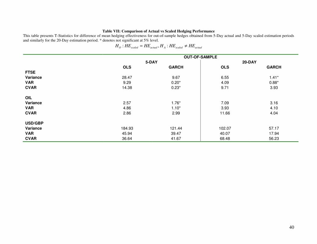
Looking now at comparisons between the actual and scaled hedges for the out-of-

sample hedges, we find that there are significant statistical differences in 83% of cases

across assets and frequencies. At the 5-Day hedging horizon, the actual hedges

25

outperform the scaled hedges for FTSE and USD/GBP, whereas for Oil the scaled

hedges generally yield lower risk. However the differences again are only economically

significant for the USD/GBP contract. When we examine the 20-Day hedges, we find

that the actual hedges are the best performers for all assets but again the differences

are only economically significant for the USD/GBP contract. For example, using a

$1,000,000 exposure to illustrate, the difference between the CVaR of the USD/GBP

hedge calculated directly is $6,800 lower than the CVaR of the scaled hedge. This

represents a difference of 81% in favour of the actual hedge.

In terms of hedging models, there are generally no significant differences between the

OLS and the GARCH models, irrespective of whether statistical or economical

evaluation is used. The best model may change for a given asset or hedge horizon. We

also expected ex-ante that the out-of-sample performance of the GARCH model would

be relatively better as compared with the OLS model for shorter horizons because

volatility persistence is greater for high frequency data. However there is no conclusive

evidence that this is the case as the performance differential is not significantly different

for different hedge horizons. Looking at the actual risk measures, both the OLS and

GARCH models provide broadly similar performance. For the FTSE the GARCH model

appears to have the edge. It outperforms the OLS model for seven out of nine cases

across the difference frequencies and the different risk measures. The exceptions are

the VaR at the 5-day frequency and the Variance at the 20-day frequency. For the Oil

and the USUK assets, the performance is more even, and depends on the particular

risk measure and the frequency. Taking Oil, for example, the OLS yields a marginally

lower CVaR of 3.19 at the 20-day frequency as compared with 3.20 for the GARCH

model. The similarity in performance of the models is not surprising given that it relates

26

to the average performance of the hedges across time, and therefore performance

differences tend to be quite small. Note also that the variance of the hedged portfolios

tends to increase as we increase the hedging horizon. The only exception to this is for

Oil at the 5-day and 20-day frequencies and this relates to very similar performance for

these particular hedges.

VII Summary and Conclusion

This paper compares hedge strategies across three different investor time horizons. We

calculate hedges using volatility and covariance estimates based on direct estimation

and compare these with hedges obtained using scaled data. Significant differences

emerge between the hedge strategies, indicating that scaled hedges tend to be lower in

absolute value and less volatile than those obtained from direct estimation. These

differences can be traced back to the correlation properties of cash and futures which

increase as the hedging horizon lengthens. Despite these differences, scaled hedges

provide good outcomes in terms of absolute hedging effectiveness across all assets.

In terms of the relative performance of scaled versus actual hedges, for Equity Index

and Oil hedges, particularly when scaling 1-day hedges up to 1-week, the relative

performance is broadly similar. For foreign exchange hedges especially at the 20-day

frequency, the results of scaling are poor when compared with the actual hedges. We

conclude therefore that only for the foreign exchange (USD/GBP) hedges can economic

and statistical differences be called significant, therefore the broad finding is that scaling

provides reasonably good outcomes in reducing risk.

27

We also examine the temporal aggregation properties of a GARCH model using the

Drost Nyman approach which allows us to compare volatility persistence for high

frequency and low frequency data. The results show that lower levels of volatility

persistence do not materially affect the ex-post hedging effectiveness at lower

frequencies. We also provide further evidence that ex-post hedging effectiveness

increases as we move from high to low frequency hedging. The implications of our

findings are twofold. Firstly, scaling provides good absolute, and reasonable relative

hedging outcomes vis a vis direct estimation while avoiding some of the statistical

problems associated with direct estimation at low frequencies. Furthermore, it is

particularly useful for assets such as equity index hedges and for relatively short time

scales such as 1-day to 5-day. For time scales such as 20-day or longer, the findings

seem to suggest that constant or average OHR’s approach the Naïve hedge ratio of 1,

and therefore it may be that this approach may prove suitable for hedges based on time

horizons longer than 1-month.

28

Bibliography

Anderson, T., Bollerslev, T., Diebold, F., & Ebens, H. (2001). The distribution of realised

stock return volatility. Journal of Financial Economics, 61, 43 – 76.

Basel Committee on Banking Supervision, 2004. International convergence of capital

measurement and capital standards: A revised framework. Bank for International

Settlements.

Bauwens, L., Laurent, S., & Rombouts, K. (2006.) Multivariate Garch Models: A Survey.

Journal of Applied Econometrics. 21, 79 – 109.

Bollerslev, T., Chou, R., & Kroner, K. (1992). ARCH modelling in finance. A review of

the theory & empirical evidence. Journal of Econometrics, 52, 5 – 59.

Bollerslev, T., R. Engle, & J. Wooldridge, 1988, “A Capital Asset Pricing Model with

Time-Varying Covariances,” Journal of Political Economy 96, 116 - 131.

Brock, W. (1999). Scaling in economics: A readers guide, Technical Report 9912,

University of Wisconsin, Department. of Economics, Madison, WI.

Brummelhuis, R. & Kaufmann, R. (2007). Time Scaling of Value-at-Risk in GARCH (1,

1) and AR (1)-GARCH (1, 1) Processes. The Journal of Risk, 9, 39-94.

29

Chen, S., Lee, C., & Shrestha, K. (2004). An empirical analysis of the relationship

between the hedge ratio and hedging horizon: a simultaneous estimation of the short

and long run hedge ratios. The Journal of Futures Markets, 24, 359 – 386.

Christoffersen, P., Diebold, F., & Schuermann, T. (1998). Horizon problems and

extreme events in financial risk management. Economic Policy Review, Federal

Reserve Bank of New York, 109-118.

Christoffersen, P., & Diebold, F. (2000). How Relevant is Volatility Forecasting for

Financial Risk Management. Review of Economics and Statistics, 82, 12-22.

Cotter, J., & Dowd, K. (2006). Extreme spectral risk measures: An application to futures

clearing house margin requirements. Journal of Banking and Finance, 30, 3469-3485.

Cotter, J., & Hanly, J. (2006). Re-examining hedging performance. Journal of Futures

Markets, 26, 657-676.

Dacarogna, M., Muller, U., Pictet, O. & de Vries, C. (1998). Extremal forex returns in

extremely large data sets. Tinbergen Institute.

Dacarogna, M., Gencay, R., Muller, U., Olsen, R. & Pictet, O. (2001). An introduction to

high frequency finance. 1st Edition, Academic Press.

Danielsson, J., & Zigrand, J. (2006). On time-scaling of risk and the square-root-of-time

rule. Journal of Banking and Finance, 30, 2701-2713.

30

Diebold, F., Hickman, A., Inoue, A. & Schuermann, T. (1998). Converting 1-day volatility

to h-day volatility: scaling by root-h is worse than you think. Wharton Financial

Institutions Centre, Working Paper No. 97-34.

Dowd, K., & Oliver, P. (2006). Temporal Aggregation of GARCH Volatility Processes: A

(Partial) Rehabilitation of the Square-Root Rule. Journal of Accounting and Finance, 5,

51-60.

Drost, F., & Nijman, T. (1993). Temporal aggregation of GARCH processes.

Econometrica, 61, 909-927.

Ederington, L., (1979). The hedging performance of the new futures markets. The

Journal of Finance, 34, 157 – 170.

Efron, B., (1979), “Bootstrap Methods: Another Look at the Jack-Knife,” The Annals of

Statistics 7, 1–26.

Engle, R., (1982), “Autoregressive conditional heteroskedasticity with estimates of the

variance of United Kingdom Inflation,” Econometrica, 50, 987 – 1008.

Geppert, J., (1995). A statistical model for the relationship between futures contract

hedging effectiveness and investment horizon length. The Journal of Futures Markets,

15, 507 – 536.

Hull, J. (2008). Options futures and other derivatives. 7th Edition, Prentice Hall.

31

Hwang, S., & Valls Pereira, P. (2006). Small sample properties of GARCH estimates

and persistence. The European Journal of Finance, 12, 473 – 494.

In, F., & Kim, S. (2006). The hedge ratio and the empirical relationship between stock

and futures markets: a new approach using wavelet analysis. Journal of Business, 79,

799 – 820.

Kaufmann, R., & Patie, P. (2003). Strategic long-term financial risks: the one-

dimensional case. RiskLab Report, ETH Zurich.

Kwiatkowski, D., Phillips, P., Schmidt, P., & Shin, Y. (1992). Testing the null of

stationarity against the alternative of a unit root: How sure are we that economic time

series have unit root? Journal of Econometrics, 54, 159 – 178.

Lien, D., & Shrestha, K. (2007). An empirical analysis of the relationship between hedge

ratio and hedging horizon using wavelet analysis. The Journal of Futures Markets, 27,

127 – 150.

Lien, D., & Y. Tse, (2002). Some Recent Developments in Futures Hedging, Journal of

Economic Surveys 16, 357 – 396.

Locke, J., (1999). Riskmetrics launches new system for corporate users. Risk, 12, 54 –

55.

32

Malliaris, A., & Urrutia, J. (1991). The impact of the lengths of estimation periods and

hedging horizons on the effectiveness of a hedge: evidence from foreign currency

futures. The Journal of Futures Markets, 11, 271 – 289.

Mandelbrot, B. (1963). The variation of certain speculative prices. Journal of Business,

36, 394 - 419

Merton, R., (1980). On estimating the expected return on the market: an exploratory

investigation. Journal of Financial Economics, 8, 323 – 361.

Poon, S., & Granger, W. (2003). Forecasting volatility in financial markets: A review.

Journal of Economic Literature, 61, 478 – 539.

Smithson, C., & Minton, L. (1996). Value-at-Risk. Risk, 9, 38 – 39.

33

Table I: Descriptive Statistics This table presents summary statistics for the log returns of each cash and futures series. The Mean and Standard Deviation (SD) are expressed as percentages. A comparison of the scaled and the actual data shows that as we scale the 1-day standard deviations to the 5-day frequency using the SQRT rule, the average deviation of the scaled standard deviation as compared with the actual standard deviation across all assets would be just 1.14% however at the 20-day frequency the average difference rises to 7.7%. This indicates that scaling provides a good approximation up to a factor of five but that it declines rapidly thereafter. The excess skewness statistic measures asymmetry where zero would indicate a symmetric distribution. The excess kurtosis statistic measures the shape of a distribution where a value of zero would indicate a normal distribution. The Jarque and Bera (J-B) statistic measures normality. LM with 4 lags is the Lagrange Multiplier test for ARCH effects proposed by Engle 1982 and is distributed as χ

2. Stationarity is tested using the KPSS test which tests the null of stationarity against the alternative of a unit root. Critical Values for the KPSS test at the 1% level are 0.739 and 0.216 for the constant and trend statistics respectively. The correlation coefficient between each set of cash and futures is also given. Associated p-Values are given in brackets.

1-Day 5-Day 20-Day

Cash Futures Cash Futures Cash Futures

FTSE 100

Mean 0.009 0.009 0.052 0.051 0.23 0.22

SD 1.11 1.18 2.47 2.56 4.67 4.78

SD Scaled 2.48 2.64 4.96 5.28

Skewness -0.166

(0.00)

-0.086

(0.00)

-0.578

(0.00)

-0.496

(0.00)

-0.402

(0.06)

-0.405

(0.06)

Kurtosis 2.87

(0.00)

2.29

(0.00)

3.12

(0.00)

2.85

(0.00)

0.71

(0.00)

0.55

(0.00)

J-B 916.94

(0.00)

579.29

(0.00)

241.04

(0.00)

197.78

(0.00)

18.30

(0.00)

14.78

(0.00)

LM 463.31

(0.00)

410.82

(0.00)

29.56

(0.00)

25.99

(0.00)

14.89

(0.01)

14.35

(0.01)

KPSS - Constant

- Trend

0.513

0.096

0.484

0.092

0.585

0.114

0.570

0.113

0.606

0.138

0.302

0.139

Correlation 0.970 0.988 0.992

OIL

Mean 0.016 0.016 0.069 0.066 0.26 0.26

SD 2.34 2.21 5.16 5.08 9.41 9.52

SD Scaled 5.23 4.94 10.46 9.88

Skewness -0.321

(0.00)

-0.251

(0.00)

-0.537

(0.00)

-0.577

(0.00)

-0.044

(0.83)

-0.149

(0.48)

Kurtosis 5.07

(0.00)

4.54

(0.00)

3.08

(0.00)

3.09

(0.00)

0.353

(0.42)

0.433

(0.32)

J-B 2857.03

(0.00)

2283.23

(0.00)

231.29

(0.00)

237.14

(0.00)

0.72

(0.69)

1.51

(0.46)

LM 65.03

(0.00)

43.47

(0.00)

4.39

(0.35)

3.79

(0.43)

5.74

(0.21)

6.83

(0.14)

KPSS - Constant

- Trend

0.063

0.032

0.069

0.035

0.066

0.041

0.064

0.041

0.071

0.048

0.072

0.048

Correlation 0.876 0.971 0.993

USD/GBP

Mean 0.003 0.003 0.011 0.011 0.040 0.042

SD 0.48 0.51 1.06 1.10 2.05 1.99

SD Scaled 1.07 1.14 2.15 2.28

Skewness 0.0175

(0.71)

0.0152

(0.74)

-0.103

(0.33)

-0.181

(0.09)

-0.024

(0.90)

0.020

(0.92)

Kurtosis 1.92

(0.00)

2.72

(0.00)

0.30

(0.15)

0.25

(0.23)

0.65

(0.13)

0.88

(0.04)

J-B 402.53

(0.00)

812.74

(0.00)

2.95

(0.22)

4.28

(0.12)

2.32

(0.31)

4.24

(0.12)

LM

18.10

(0.00)

9.18

(0.05)

14.74

(0.10)

9.67

(0.10)

3.14

(0.53)

3.44

(0.48)

KPSS - Constant

- Trend

0.056

0.043

0.056

0.041

0.069

0.057

0.072

0.055

0.104

0.085

0.111

0.086

Correlation 0.816 0.949 0.989

34

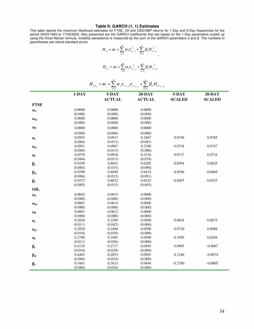
Table II: GARCH (1, 1) Estimates This table reports the maximum likelihood estimates for FTSE, Oil and USD/GBP returns for 1-Day and 5-Day frequencies for the period 29/03/1993 to 17/03/2003. Also presented are the GARCH coefficients that are based on the 1-Day parameters scaled up using the Drost Nijman formula. Volatility persistence is measured by the sum of the GARCH parameters α and β. The numbers in parentheses are robust standard errors.

∑∑=

−=

−++=

n

kktsk

m

jjtsjts HH

1

2

1

2βεαω

,

∑∑=

−=

−++=

n

kktfk

m

jjtfjtf HH

1

2

1

2βεαω

∑∑=

−−=

−++=

n

kktsfkjtf

m

jjtsjtsf HH

11

βεεαω

1-DAY 5-DAY 20-DAY 5-DAY 20-DAY

ACTUAL ACTUAL SCALED SCALED

FTSE

ωs 0.0000

(0.000)

0.0000

(0.000)

0.0000

(0.000)

ωsf 0.0000

(0.000)

0.0000

(0.000)

0.0000

(0.000)

ωf 0.0000 0.0000 0.0000

(0.000) (0.000) (0.000)

αs 0.0565

(0.004)

0.0913

(0.013)

0.2467

(0.081)

0.0746

0.0785

αsf 0.0561

(0.004)

0.0907

(0.013)

0.2380

(0.080)

0.0734

0.0747

αf 0.0570

(0.004)

0.0910

(0.013)

0.2318

(0.078)

0.0737

0.0734

βs 0.9299

(0.004)

0.8841

(0.015)

0.6285

(0.090)

0.8594

0.6825

βsf 0.9290

(0.004)

0.8840

(0.015)

0.6414

(0.091)

0.8546

0.6669

βf 0.9272

(0.005)

0.8832

(0.015)

0.6525

(0.093)

0.8497

0.6535

OIL

ωs 0.0002

(0.000)

0.0015

(0.000)

0.0000

(0.000)

ωsf 0.0001

(0.000)

0.0014

(0.000)

0.0000

(0.000)

ωf 0.0001

(0.000)

0.0012

(0.000)

0.0000

(0.000)

αs 0.2836

(0.011)

0.2569

(0.042)

0.0500

(0.000)

0.0654

0.0075

αsf 0.2820

(0.010)

0.2494

(0.038)

0.0500

(0.000)

0.0720

0.0088

αf 0.2780

(0.011)

0.2465

(0.036)

0.0500

(0.000)

0.1056

0.0204

βs 0.4129

(0.010)

0.2717

(0.028)

0.0495

(0.000)

0.0985

-0.0067

βsf 0.4403

(0.006)

0.2853

(0.024)

0.0503

(0.000)

0.1246

-0.0074

βf 0.5441

(0.006)

0.3615

(0.026)

0.0494

(0.000)

0.2700

-0.0005

35

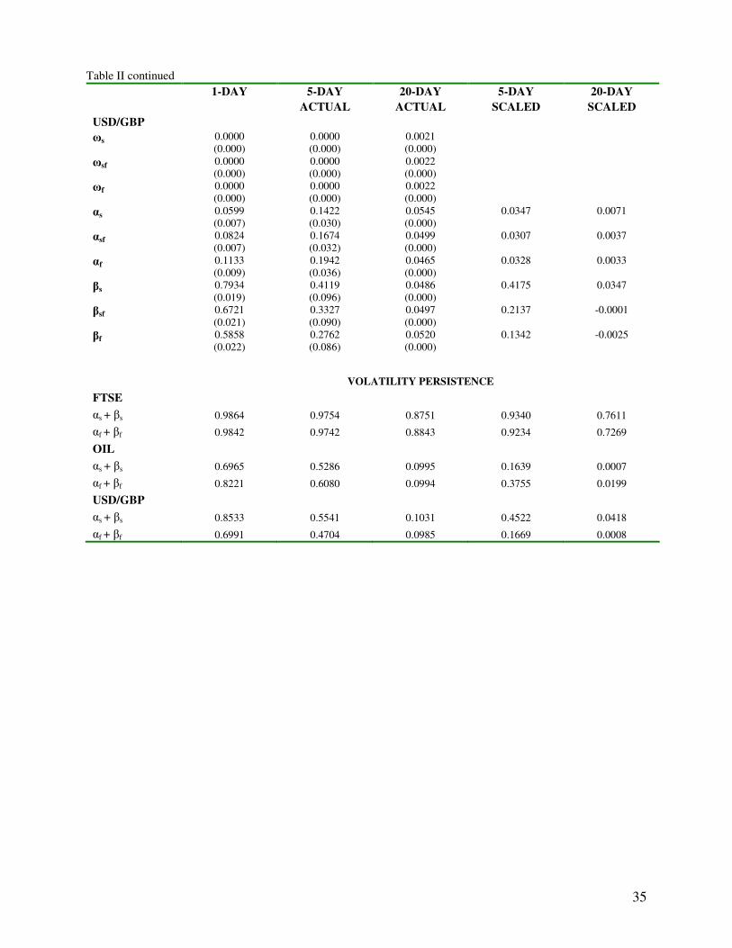
Table II continued

1-DAY 5-DAY 20-DAY 5-DAY 20-DAY

ACTUAL ACTUAL SCALED SCALED

USD/GBP

ωs 0.0000

(0.000)

0.0000

(0.000)

0.0021

(0.000)

ωsf 0.0000

(0.000)

0.0000

(0.000)

0.0022

(0.000)

ωf 0.0000

(0.000)

0.0000

(0.000)

0.0022

(0.000)

αs 0.0599

(0.007)

0.1422

(0.030)

0.0545

(0.000)

0.0347

0.0071

αsf 0.0824

(0.007)

0.1674

(0.032)

0.0499

(0.000)

0.0307

0.0037

αf 0.1133

(0.009)

0.1942

(0.036)

0.0465

(0.000)

0.0328

0.0033

βs 0.7934

(0.019)

0.4119

(0.096)

0.0486

(0.000)

0.4175

0.0347

βsf 0.6721

(0.021)

0.3327

(0.090)

0.0497

(0.000)

0.2137

-0.0001

βf 0.5858

(0.022)

0.2762

(0.086)

0.0520

(0.000)

0.1342

-0.0025

VOLATILITY PERSISTENCE

FTSE

αs + βs 0.9864 0.9754 0.8751 0.9340 0.7611

αf + βf 0.9842 0.9742 0.8843 0.9234 0.7269

OIL

αs + βs 0.6965 0.5286 0.0995 0.1639 0.0007

αf + βf 0.8221 0.6080 0.0994 0.3755 0.0199

USD/GBP

αs + βs 0.8533 0.5541 0.1031 0.4522 0.0418

αf + βf 0.6991 0.4704 0.0985 0.1669 0.0008

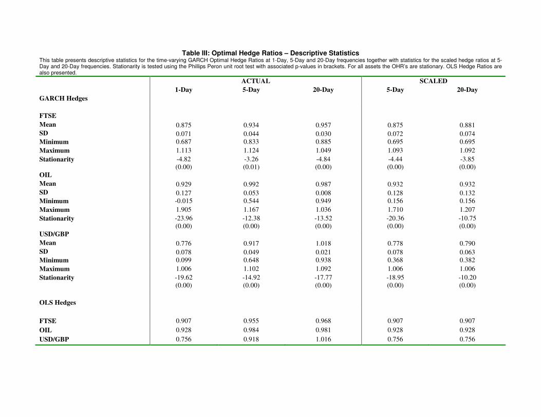
Table III: Optimal Hedge Ratios – Descriptive Statistics This table presents descriptive statistics for the time-varying GARCH Optimal Hedge Ratios at 1-Day, 5-Day and 20-Day frequencies together with statistics for the scaled hedge ratios at 5-Day and 20-Day frequencies. Stationarity is tested using the Phillips Peron unit root test with associated p-values in brackets. For all assets the OHR’s are stationary. OLS Hedge Ratios are also presented.

ACTUAL SCALED

1-Day 5-Day 20-Day 5-Day 20-Day

GARCH Hedges

FTSE

Mean 0.875 0.934 0.957 0.875 0.881

SD 0.071 0.044 0.030 0.072 0.074

Minimum 0.687 0.833 0.885 0.695 0.695

Maximum 1.113 1.124 1.049 1.093 1.092

Stationarity -4.82

(0.00)

-3.26

(0.01)

-4.84

(0.00)

-4.44

(0.00)

-3.85

(0.00)

OIL

Mean 0.929 0.992 0.987 0.932 0.932

SD 0.127 0.053 0.008 0.128 0.132

Minimum -0.015 0.544 0.949 0.156 0.156

Maximum 1.905 1.167 1.036 1.710 1.207

Stationarity -23.96

(0.00)

-12.38

(0.00)

-13.52

(0.00)

-20.36

(0.00)

-10.75

(0.00)

USD/GBP

Mean 0.776 0.917 1.018 0.778 0.790

SD 0.078 0.049 0.021 0.078 0.063

Minimum 0.099 0.648 0.938 0.368 0.382

Maximum 1.006 1.102 1.092 1.006 1.006

Stationarity

-19.62

(0.00)

-14.92

(0.00)

-17.77

(0.00)

-18.95

(0.00)

-10.20

(0.00)

OLS Hedges

FTSE 0.907 0.955 0.968 0.907 0.907

OIL 0.928 0.984 0.981 0.928 0.928

USD/GBP 0.756 0.918 1.016 0.756 0.756

37

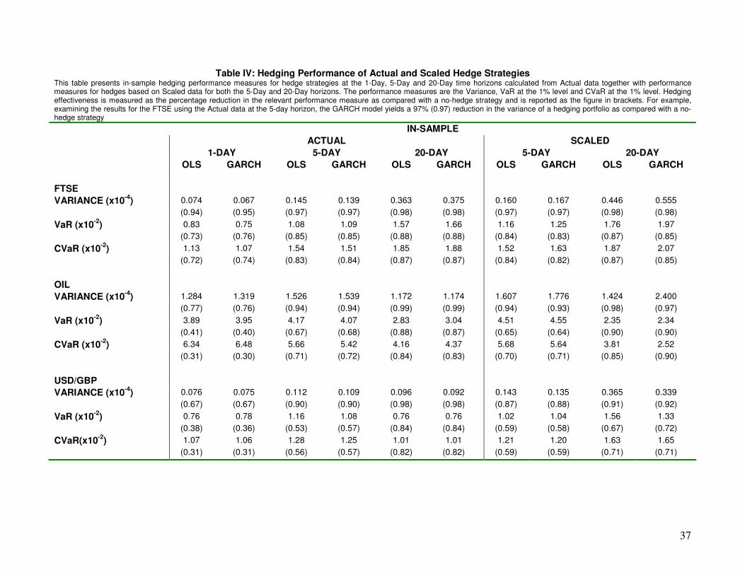
Table IV: Hedging Performance of Actual and Scaled Hedge Strategies This table presents in-sample hedging performance measures for hedge strategies at the 1-Day, 5-Day and 20-Day time horizons calculated from Actual data together with performance measures for hedges based on Scaled data for both the 5-Day and 20-Day horizons. The performance measures are the Variance, VaR at the 1% level and CVaR at the 1% level. Hedging effectiveness is measured as the percentage reduction in the relevant performance measure as compared with a no-hedge strategy and is reported as the figure in brackets. For example, examining the results for the FTSE using the Actual data at the 5-day horizon, the GARCH model yields a 97% (0.97) reduction in the variance of a hedging portfolio as compared with a no-hedge strategy

IN-SAMPLE

ACTUAL SCALED

1-DAY 5-DAY 20-DAY 5-DAY 20-DAY

OLS GARCH OLS GARCH OLS GARCH OLS GARCH OLS GARCH

FTSE

VARIANCE (x10-4

) 0.074 0.067 0.145 0.139 0.363 0.375 0.160 0.167 0.446 0.555

(0.94) (0.95) (0.97) (0.97) (0.98) (0.98) (0.97) (0.97) (0.98) (0.98)

VaR (x10-2

) 0.83 0.75 1.08 1.09 1.57 1.66 1.16 1.25 1.76 1.97

(0.73) (0.76) (0.85) (0.85) (0.88) (0.88) (0.84) (0.83) (0.87) (0.85)

CVaR (x10-2

) 1.13 1.07 1.54 1.51 1.85 1.88 1.52 1.63 1.87 2.07

(0.72) (0.74) (0.83) (0.84) (0.87) (0.87) (0.84) (0.82) (0.87) (0.85)

OIL

VARIANCE (x10-4

) 1.284 1.319 1.526 1.539 1.172 1.174 1.607 1.776 1.424 2.400

(0.77) (0.76) (0.94) (0.94) (0.99) (0.99) (0.94) (0.93) (0.98) (0.97)

VaR (x10-2

) 3.89 3.95 4.17 4.07 2.83 3.04 4.51 4.55 2.35 2.34

(0.41) (0.40) (0.67) (0.68) (0.88) (0.87) (0.65) (0.64) (0.90) (0.90)

CVaR (x10-2

) 6.34 6.48 5.66 5.42 4.16 4.37 5.68 5.64 3.81 2.52

(0.31) (0.30) (0.71) (0.72) (0.84) (0.83) (0.70) (0.71) (0.85) (0.90)

USD/GBP

VARIANCE (x10-4

) 0.076 0.075 0.112 0.109 0.096 0.092 0.143 0.135 0.365 0.339

(0.67) (0.67) (0.90) (0.90) (0.98) (0.98) (0.87) (0.88) (0.91) (0.92)

VaR (x10-2

) 0.76 0.78 1.16 1.08 0.76 0.76 1.02 1.04 1.56 1.33

(0.38) (0.36) (0.53) (0.57) (0.84) (0.84) (0.59) (0.58) (0.67) (0.72)

CVaR(x10-2

) 1.07 1.06 1.28 1.25 1.01 1.01 1.21 1.20 1.63 1.65

(0.31) (0.31) (0.56) (0.57) (0.82) (0.82) (0.59) (0.59) (0.71) (0.71)

38

Table V: Comparison of Actual vs Scaled Hedging Performance

This table presents t-Statistics for difference of mean hedging effectiveness for in-sample hedges obtained from 5-Day actual and 5-Day scaled estimation periods and

similarly for the 20-Day estimation period. * denotes not significant at 5% level.

actualscaledAactualscaledO HEHEHHEHEH ≠= :,:

IN-SAMPLE

5-DAY 20-DAY

OLS GARCH OLS GARCH

FTSE

Variance 10.60 19.57 6.93 13.37

VAR 5.16 10.05 3.75 7.34

CVAR 1.57* 8.94 0.88* 9.07

OIL

Variance 4.37 12.16 4.34 11.34

VAR 5.27 6.38 3.04 6.17

CVAR 0.30* 0.35* 2.74 25.07

USD/GBP

Variance 120.91 85.44 114.95 94.77

VAR 25.54 21.61 44.00 37.10

CVAR 14.39 18.53 65.62 75.67

39

Table VI: Hedging Performance of Actual and Scaled Hedge Strategies This table presents out-of-sample hedging performance measures for hedge strategies at the 1-Day, 5-Day and 20-Day time horizons calculated from Actual data together with performance measures for hedges based on Scaled data for both the 5-Day and 20-Day horizons. The performance measures are the Variance, VaR at the 1% level and CVaR at the 1% level. Hedging effectiveness is measured as the percentage reduction in the relevant performance measure as compared with a no-hedge strategy and is reported as the figure in brackets. For example, examining the results for the FTSE, using the Scaled data at the 20-day horizon, the GARCH model yields a 98% (0.98) reduction in the variance of a hedging portfolio as compared with a no-hedge strategy

OUT-OF-SAMPLE

ACTUAL SCALED

1-DAY 5-DAY 20-DAY 5-DAY 20-DAY

OLS GARCH OLS GARCH OLS GARCH OLS GARCH OLS GARCH

FTSE

VARIANCE (x10-4

) 0.031 0.026 0.052 0.046 0.137 0.146 0.080 0.052 0.174 0.155

(0.96) (0.97) (0.99) (0.99) (0.98) (0.98) (0.98) (0.99) (0.98) (0.98)

VaR (x10-2

) 0.51 0.48 0.64 0.65 0.95 0.92 0.75 0.64 0.85 0.94

(0.81) (0.81) (0.89) (0.89) (0.86) (0.87) (0.87) (0.89) (0.88) (0.86)

CVaR (x10-2

) 0.67 0.65 0.83 0.78 1.02 0.99 1.06 0.78 0.85 1.05

(0.79) (0.80) (0.89) (0.90) (0.88) (0.88) (0.86) (0.90) (0.90) (0.88)

OIL

VARIANCE (x10-4

) 0.720 0.728 1.184 1.239 1.156 1.141 1.231 1.207 1.584 1.305

(0.83) (0.83) (0.94) (0.94) (0.98) (0.98) (0.94) (0.94) (0.97) (0.98)

VaR (x10-2

) 2.91 2.98 3.98 3.94 3.09 2.91 3.74 3.89 3.50 3.30

(0.44) (0.42) (0.62) (0.63) (0.79) (0.80) (0.65) (0.63) (0.77) (0.78)

CVaR (x10-2

) 4.71 4.78 4.57 4.62 3.19 3.20 4.44 4.48 3.64 3.36

(0.27) (0.26) (0.69) (0.69) (0.80) (0.80) (0.70) (0.70) (0.77) (0.79)

USD/GBP

VARIANCE (x10-4

) 0.060 0.056 0.117 0.113 0.127 0.131 0.179 0.142 0.554 0.385

(0.78) (0.79) (0.91) (0.92) (0.98) (0.98) (0.87) (0.90) (0.90) (0.93)

VaR (x10-2

) 0.60 0.59 0.89 0.89 0.68 0.76 1.13 1.05 1.37 1.15

(0.56) (0.57) (0.65) (0.65) (0.85) (0.84) (0.55) (0.58) (0.71) (0.75)

CVaR(x10-2

) 0.91 0.89 1.12 1.11 0.84 0.83 1.37 1.27 1.52 1.32

(0.42) (0.44) (0.67) (0.67) (0.83) (0.83) (0.59) (0.62) (0.69) (0.73)

40

Table VII: Comparison of Actual vs Scaled Hedging Performance

This table presents T-Statistics for difference of mean hedging effectiveness for out-of-sample hedges obtained from 5-Day actual and 5-Day scaled estimation periods

and similarly for the 20-Day estimation period. * denotes not significant at 5% level.

actualscaledAactualscaledO HEHEHHEHEH ≠= :,:

OUT-OF-SAMPLE

5-DAY 20-DAY

OLS GARCH OLS GARCH

FTSE

Variance 28.47 9.67 6.55 1.41*

VAR 9.29 0.20* 4.09 0.88*

CVAR 14.38 0.23* 9.71 3.93

OIL

Variance 2.57 1.76* 7.09 3.16

VAR 4.86 1.10* 3.93 4.10

CVAR 2.86 2.99 11.66 4.04

USD/GBP

Variance 184.93 121.44 102.07 57.17

VAR 45.94 39.47 40.07 17.94

CVAR 36.64 41.67 68.48 56.23

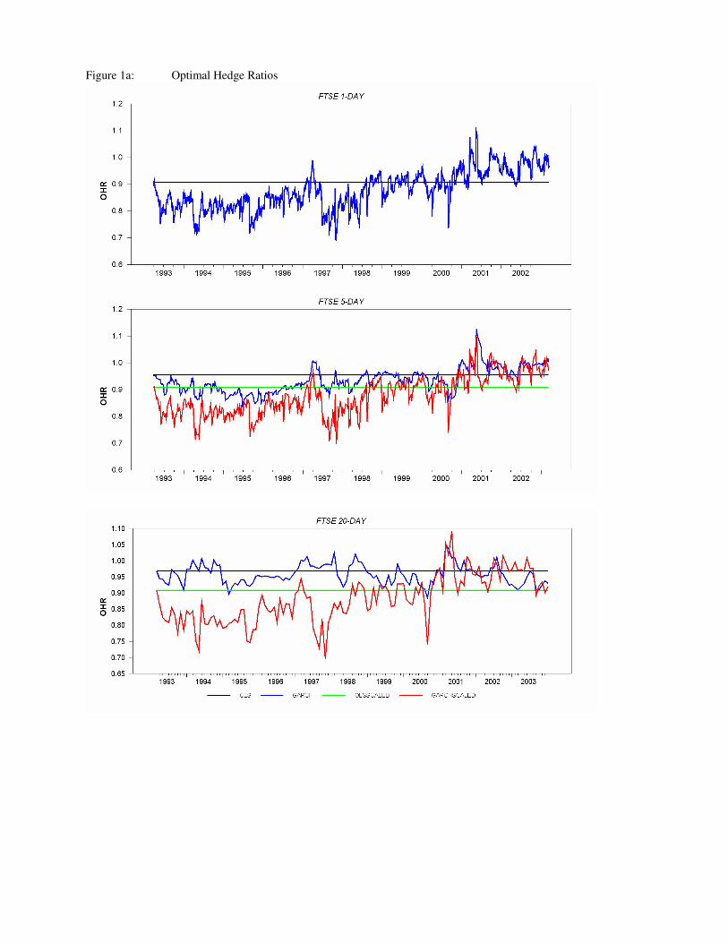
Figure 1a: Optimal Hedge Ratios

42

Figure 1b: Optimal Hedge Ratios

43

Figure 1c: Optimal Hedge Ratios