SverigeS rikSbankworking paper SerieS 206

optimal Monetary policy under Downward nominal wage rigidity

Mikael Carlsson and Andreas Westermarkapril 2007

working paperS are obtainable froM

Sveriges riksbank • information riksbank • Se-103 37 Stockholmfax international: +46 8 787 05 26

telephone international: +46 8 787 01 00e-mail: info@riksbank.se

the working paper series presents reports on matters in the sphere of activities of the riksbank that are considered

to be of interest to a wider public.the papers are to be regarded as reports on ongoing studies

and the authors will be pleased to receive comments.

the views expressed in working papers are solely the responsibility of the authors and should not to be interpreted as

reflecting the views of the executive board of Sveriges riksbank.

Optimal Monetary Policy under Downward Nominal Wage Rigidity∗

Mikael Carlsson†and Andreas Westermark‡

Sveriges Riksbank Working Paper Series

No. 206

Revised November 2007

Abstract

We develop a New Keynesian model with staggered price and wage setting where downward

nominal wage rigidity (DNWR) arises endogenously through the wage bargaining institutions. It is

shown that the optimal (discretionary) monetary policy response to changing economic conditions

then becomes asymmetric. Interestingly, in our baseline model we find that the welfare loss is

actually slightly smaller in an economy with DNWR. This is due to that DNWR is not an additional

constraint on the monetary policy problem. Instead, it is a constraint that changes the choice set

and opens up for potential welfare gains due to lower wage variability. Another finding is that the

Taylor rule provides a fairly good approximation of optimal policy under DNWR. In contrast, this

result does not hold in the unconstrained case. In fact, under the Taylor rule, agents would clearly

prefer an economy with DNWR before an unconstrained economy ex ante.

Keywords: Monetary Policy; Wage Bargaining; Downward Nominal Wage Rigidity.

JEL classification: E52, E58, J41.

∗We are grateful to Nobuhiro Kiyotaki, Mathias Trabandt and seminar participants at Sveriges Riksbank, NorgesBank, Uppsala University, the 2006 Meeting of the European Economic Association, Vienna, and the 2007 North Amer-ican Winter Meeting of The Econometric Society, Chicago, for useful comments. We would also like to thank Erikvon Schedvin for excellent research assistance. We gratefully acknowledge financial support from Jan Wallander’s andand Tom Hedelius’ Research Foundation and Westermark also from the Swedish Council for Working Life and SocialResearch. The views expressed in this paper are solely the responsibility of the authors and should not be interpretedas reflecting the views of the Executive Board of Sveriges Riksbank.

†Research Department, Sveriges Riksbank, SE-103 37, Stockholm, Sweden. e-mail: mikael.carlsson@riksbank.se.‡Department of Economics, Uppsala University, P.O. Box 513, SE-751 20 Uppsala, Sweden. e-mail:

andreas.westermark@nek.uu.se.

1

Introduction

A robust empirical finding is that money wages do not fall during an economic downturn, at least

not to any significant degree. A large number of studies report substantial downward nominal wage

rigidity in the U.S. as well as in Europe and Japan.1 Overall, the evidence points towards a sharp

asymmetry in the distribution of nominal wage changes around zero. That is, money wages rise but

they seldom fall. This may not have any noticeable real effects in periods with sufficiently high inflation

rates to allow for a reduction of real wages in response to adverse shocks without reducing nominal

wages. However, inflation rates have come down in many countries in recent decade(s) and periods

of very low inflation rates are no longer out of the picture. Recent examples are Japan, Sweden and

Switzerland which have all experienced prolonged episodes with average CPI-inflation rates below one

percent (see below). Still, downward nominal wage rigidity may not be a concern for real outcomes, if

it is not a feature of low inflation environments, as conjectured by e.g. Gordon (1996). However, the

empirical evidence shows that the downward rigidity of nominal wages persists even in low inflation

environments (see Agell and Lundborg, 2003, Fehr and Goette, 2005, and Kuroda and Yamamoto

2003a, 2003b). This, in turn, opens up for potentially important real effects of downward nominal

wage rigidity in the current era of low inflation rates.

The purpose of this paper is to study the implications for monetary policy in situations where

declining nominal wages are not a viable margin for adjustment to adverse economic conditions. To

this end, we develop a New Keynesian DSGE model that can endogenously account for downward

nominal wage rigidity. More specifically, this is achieved by introducing wage bargaining between

firms and unions as is done in Carlsson and Westermark (2006a), but modified in line with Holden

(1994). Then, downward nominal wage rigidity arises as a rational outcome.

In the model, price and wage setting are staggered. The main difference with our approach, relative

to standard New Keynesian DSGE models including an explicit labor market (see Erceg, Henderson

and Levin, 2000) is that we model wages as being determined in bargaining between firms and unions

(households).2 We follow Carlsson andWestermark (2006a), and assume that the household is attached

to a firm.

Wage bargaining is opened with a fixed probability each period, akin to Calvo (1983). Moreover,

1The empirical evidence ranges from studies using data from personnel files presented in Altonji and Devereux (2000),Baker, Gibbs, and Holmstrom (1994), Fehr and Goette (2005), and Wilson (1999), survey/register data in Altonji andDevereux (2000), Akerlof, Dickens, and Perry (1996), Dickens, Goette, Groshen, Holden, Messina, Schweitzer, Turunen,and Ward (2006), Fehr and Goette (2005), Holden and Wulfsberg (2007), Kuroda and Yamamoto (2003a, 2003b) tointerviews or surveys with wage setters like Agell and Lundborg (2003), and Bewley (1999), just to mention a few.

2For this purpose, we must modify the simplifying assumption of Erceg, Henderson, and Levin (2000), that allhouseholds work at all firms. Otherwise, each individual household works an infinitesimal amount at each firm, implyingthat the effect of the individual household’s wage on firm surplus is zero. Thus, in the standard setup, there is no surplusto be negotiated over, hence rendering bargaining irrelevant.

2

bargaining is non-cooperative as in the Rubinstein-Ståhl model, with the addition that if there is

disagreement but no party is willing to call a conflict, work takes place according to the old contract.

As argued by Holden (1994), this is in line with the labor market institutions in the U.S. and most

western European countries. Moreover, as in Holden (1994), there are costs associated with conflicts

in addition to costs stemming from impatience, such as disruptions in business relationships, startup

costs and deteriorating management-employee relationships. These costs sometimes render threats

of conflict non-credible, leading to agreement on the same wage as in the old contract. Since it is

reasonable to assume that these costs are much larger for firms than for workers, workers can credibly

threaten firms with conflict, whereas firms cannot. Since workers only use the threat to bid up wages,

downward nominal wage rigidity will result.

Given our setup, a non-linear restriction on wage inflation due to downward nominal wage rigidity

arises endogenously. Then, given the constraints from private sector behavior, the central bank solves

for optimal (discretionary) monetary policy.3

The optimal response to changing economic conditions is asymmetric, and not only in the wage

inflation dimension. Interestingly, the welfare loss is actually slightly smaller in an economy with

downward nominal wage rigidities in our baseline case. The reason is that downward nominal rigidity

is not an additional constraint on the problem. Instead, it is a constraint that changes the choice

set and opens up for potential welfare gains. Another finding is that the Taylor rule estimated by

Rudebusch (2002), provides a fairly good approximation of optimal discretionary policy in terms of

welfare under downward nominal wage rigidity. Experimenting with using the original Taylor (1993)

parameters for the Taylor rule indicates that the exact specification of the Taylor rule actually plays a

minor role for this property. In contrast, neither of these results seem to hold in the unconstrained case.

A corollary is that, under the Taylor rule, agents would clearly prefer an economy with downward

nominal wage rigidities to an unconstrained economy ex ante. That is, downward nominal wage

rigidity actually helps stabilizing the economy in the wage inflation dimension, whereas it does not

induce much more variation in inflation and the output gap.

In sections 1 and 2, we outline the model and discuss the equilibrium, respectively. In section 3,

we characterize the policy problem facing the central bank. Section 4 discusses optimal policy paths

for endogenous variables as well as the welfare implications of downward nominal wage rigidity under

optimal policy. Moreover, we also discuss the outcome of using a simple instrument (Taylor) rule

instead of the optimal policy. Finally, section 5 concludes.

3We focus on the discretionary policy case, since this is closest to the actual practice of central banks.

3

1 The Economic Environment

The model outlined below is in many respects similar to that in Erceg, Henderson, and Levin (2000).

Goods are produced by monopolistically competitive producers using capital and labor. Producers set

prices in staggered contracts as in Calvo (1983). There are also some important differences, however.

In contrast to Erceg, Henderson, and Levin (2000), we follow Carlsson and Westermark (2006a),

and assume that a household is attached to each firm.4 ,5 Thus, firms do not perceive workers as

atomistic. In each period, bargaining over wages takes place with a fixed probability. Accordingly,

wages are staggered as in Calvo (1983), but, in contrast to Erceg, Henderson, and Levin (2000),

they are determined in bargaining between the household/union and the firm. Households derive

utility from consumption, real balances and leisure, earning income by working at firms and from

capital holdings. Below, we present the model in more detail and derive key relationships (for a full

derivation, see Appendix C and the Technical Appendix to Carlsson and Westermark, 2006a).

1.1 Firms and Price Setting

Since households will be identical, except for leisure choices, it simplifies the analysis to abstract away

from the households’ optimal choices for individual goods. Thus, we follow Erceg, Henderson, and

Levin (2000) and assume a competitive sector selling a composite final good, which is combined from

intermediate goods to the same proportions as those that households would choose. The composite

good is

Yt =

∙Z 1

0Yt (f)

σ−1σ

¸ σσ−1

, (1)

where σ > 1 and Yt (f) is the intermediate good produced by firm f . The price Pt of one unit of the

composite good is set equal to the marginal cost

Pt =

⎡⎣ 1Z0

Pt(f)1−σdf

⎤⎦1

1−σ

. (2)

By standard arguments, the demand function for the intermediate good f , is

Yt (f) =

µPt (f)

Pt

¶−σYt. (3)

4Several households could be attached to a firm, if these negotiate together.5There is no reallocation of workers among firms. This is obviously a simplifying assumption, but it enables us to

describe the model in terms of very simple relationships.

4

The production of firm f in period t, Yt (f), is given by the following constant returns technology

Yt (f) = AtKt (f)γ Lt (f)

1−γ , (4)

where At is the technology level common to all firms and Kt (f) and Lt (f) denote the firms’ capital

and labor input in period t, respectively. Since firms have the right to manage, Kt (f) and Lt (f) are

optimally chosen, taking the rental cost of capital and the bargained wage Wt (f) as given. Moreover,

as in Erceg, Henderson, and Levin (2000), the aggregate capital stock is fixed at K. Standard cost-

minimization arguments then imply that the marginal cost in production is given by

MCt (f) =Wt (f)

MPLt (f), (5)

where MPLt (f) is the firm’s marginal product of labor.6

1.1.1 Prices

The firm is allowed to change prices in a given period with probability 1 − α and renegotiate wages

with probability 1 − αw. In addition, any firm that is allowed to change wages is also allowed to

change prices, but not vice versa. Thus, the probability of a firm’s price remaining unchanged is αwα.

The latter assumption greatly simplifies our problem; in particular, it eliminates any intertemporal

interdependence between current and future price decisions via its effect on wage contracts for a

given firm. Besides convenience, this assumption is in line with the micro-evidence on price-setting

behavior presented in Altissimo, Ehrmann, and Smets (2006), where price and wage changes are to a

large extent synchronized in time (see especially their figure 4.4). Here, we assume that wage changes

induce price changes, since assuming the reverse would imply that the duration of wage contracts could

never be longer than the duration of prices, which seems implausible in face of the empirical evidence,

see section 3.1. Furthermore, since intertemporal interdependencies are eliminated, this allows us to

describe the goods market equilibrium by a similar type of forward looking new Keynesian Phillips

curve as in Erceg, Henderson, and Levin (2000) (see equation (21)).

The producers choose prices to maximize

maxpt(f)

Et

∞Xk=0

(αwα)kΨt,t+k [(1 + τ)Pt (f)Yt+k (f)− TC (Wt+k (f) , Yt+k (f))] (6)

s. t. Yt+k (f) =

µPt (f)

Pt+k

¶−σYt+k,

6 In contrast to Erceg, Henderson, and Levin (2000), the marginal cost is generally not equal among firms, since firmsface different wages out of steady state.

5

where TC (Wt+k (f) , yt+k (f)) denotes the cost function, Ψt+k is the households’ valuation of nominal

profits in period t+ k when in period t and τ is a tax/subsidy on output. The term inside the square

brackets is just firm profits in period t+k, given that prices were last reset in period t. The first-order

condition is

Et

∞Xk=0

(αwα)kΨt,t+k

∙σ − 1σ

(1 + τ)Pt (f)−MCt+k (f)

¸Yt+k (f) = 0. (7)

The subsidy τ is determined so as to set σ−1σ (1 + τ) = 1; that is, we assume that fiscal policy is used

to alleviate distortions due to monopoly price setting.7

1.2 Households

The economy is populated by a continuum of households, also indexed on the unit interval, which each

supplies labor to a single firm. This setup can alternatively be interpreted as a unionized economy

with firm-specific unions. In such a framework, each household can be considered as the representative

union member.

The expected life time utility of the household working at firm f in period t is given by

Et

½∞Ps=t

βs−t∙u (Cs (f)) + l

µMs (f)

Ps

¶− v (Ls (f))

¸¾, (8)

where period s utility is additively separable in three arguments, final goods consumption Cs(f), real

money balances Ms(f)Ps

, where Ms (f) denotes money holdings, and the disutility of working Ls (f).8

Finally, β ∈ (0, 1) is the household’s discount factor.

The budget constraint of the household is

δt+1,tBt (f)

Pt+

Mt (f)

Pt+ Ct (f) =

Mt−1 (f) +Bt−1 (f)

Pt+ (1 + τw)

Wt (f)Lt (f)

Pt+ΓtPt+

TtPt. (9)

The term δt+1,t represents the price vector of assets that pays one unit of currency in a particular state

of nature in the subsequent period, while the corresponding elements in Bt (f) represent the quantity

of such claims bought by the household. Moreover, Bt−1 (f) is the realization of such claims bought in

the previous period. Also, Wt (f) denotes the household’s nominal wage and τw is the tax/subsidy on

labor income. Each household owns an equal share of all firms and the aggregate capital stock. Then,

7Thus, we abstract from any Barro-Gordon type of credibility problems (see Barro and Gordon, 1983a, and Barroand Gordon, 1983b).

8 In the Technical Appendix, we also introduce a consumption shock and a labor-supply shock as in Erceg, Henderson,and Levin (2000). However, introducing these shocks does not yield any additional insights here. In fact, it can easilybe shown that under optimal policy, all disturbances in the model (introduced as in Erceg, Henderson and Levin, 2000)can be reduced to a single disturbance term (being a linear combination of all these shocks).

6

Γt is the household’s aliquot share of profits and rental income. Finally, Tt denotes nominal lump-sum

transfers from the government. As in Erceg, Henderson, and Levin (2000), we assume that there exist

complete contingent claims markets (except for leisure) and equal initial wealth across households.

Then, households are homogeneous with respect to consumption and money holdings, i.e., we have

Ct (f) = Ct, and Mt (f) =Mt for all t.

1.3 Wage Setting

When a firm/household pair is drawn to renegotiate the wage, bargaining takes place in a setup similar

to the model by Holden (1994) and is here introduced in a New Keynesian framework following Carlsson

and Westermark (2006a). There are two key features of the bargaining model in Holden (1994). First,

there are costs of invoking a conflict, which are different from the standard costs in bargaining due

to impatience. Instead, they are caused by e.g., disrupting business relationships, startup costs and

deteriorating management-employee relationships (see Holden, 1994). Second, there is an old contract

in place at the firm and if no conflict is called and no new contract is signed, the workers work

according to the old contract. As pointed out by Holden (1994), this is a common feature of many

western European countries as well as of the U.S.

The union and the firm only have incentives to call for a conflict when the negotiated contract

gives a higher payoff than the old contract. As soon as a conflict is called, payoffs are determined in a

standard Rubinstein-Ståhl bargaining game and the conflict costs are paid out of the parties’ respective

pockets. However, the costs of conflict imply that it is sometimes not credible to threaten with a

conflict in equilibrium. Specifically, if the difference between the old contract and the Rubinstein-

Ståhl solution is small relative to the conflict cost, a party cannot credibly threaten with a conflict

and force the new contract into place. Then, no new agreement is struck and work continues according

to the old contract, resulting in nominal rigidity. If the difference is sufficiently large, however, then

conflict is a credible threat. Note, though, that there will be no conflicts in equilibrium, since it is

optimal to immediately agree on the Rubinstein-Ståhl solution, rather than waiting and enduring a

conflict.9

To derive only downward nominal rigidity, asymmetries in conflict costs are required. Specifically,

if the costs are large for the firm and negligible for the union, the firm can never credibly threaten

with a conflict (at least not close to the steady state), whereas the union can always do so when the

Rubinstein-Ståhl solution is larger than the old contract. In reality, conflict costs for the workers are

probably not zero, but small. Then, wages would be adjusted only if the Rubinstein-Ståhl solution

exceeded some threshold value ω > Wt−1 (instead of ω = Wt−1). For simplicity, we restrict the

9That agreement is immediate follows from e.g. Rubinstein (1982).

7

attention to the case when conflict costs are zero for workers.10

Note that downward nominal rigidity implies that there is a potential relationship between wage

negotiations today and in the future. This interdependence comes from two sources. First, the

wage contract is a state variable in future negotiations and second, the wage set today affects prices

set in the future which, in turn, may affect future wage negotiations. The first interdependence is

eliminated by using the steady state distribution in the log linearization of the model (see Appendix

C for details and the caveat in section 2 for a further discussion). The second interdependence is

eliminated by the assumption that prices can be changed whenever wages are allowed to change.

Then, given these two steps, each wage negotiation can be analyzed separately, as in the standard

Calvo setup, thereby leading to a very simple and tractable framework. Note also that there will be

no intertemporal interdependence in price setting decisions for a given firm either. To see this, note

that since prices can be adjusted in any direction, the current price is not a state variable in future

price setting. Any interdependence in price setting over time must thus come via wage negotiations,

but such interdependence is ruled out by the assumption that prices change whenever wages change.

Unions

The union at a firm represents all workers at the firm and maximizes the welfare of all members.

Defining per-period utility (in the cash-less limiting case), for a given contract wage, as

Υt,t+k(f) = u (Ct+k)− v (Lt,t+k (f)) , (10)

where Lt,t+k (f) denotes labor demand in period t+k when prices were last reset in period t. Moreover,

let

ζt+k (dt+k(f)) = αw + (1− αw)Ft+k (dt+k(f)) , (11)

denote the probability that firm f ’s wages are unchanged in period t + k. The term Ft+k (dt+k(f))

is then firm f ’s probability that the wage is not adjusted conditional on renegotiation taking place,

which is a function of

dt+k(f) =W o

t+k (f)

Wt (f), (12)

where Wt (f) is the current contract and W ot+k (f) denotes the unconstrained optimal wage in period

t + k for firm f , defined as the wage upon which parties would agree in period t + k if all conflict

costs were temporarily removed in period t+ k. Then, let Uut+k denote union utility when the wage is

10 A full explanation of downward nominal wage rigidity is likely to include several mechanisms that may be comple-mentary. Studies like Bewley (1999), and others point towards psychological mechanisms involving fairness considerationsand managers’ concern over workplace morale. Moreover, the workers’ yardstick for fairness seems to be what happensto nominal rather than real wages. However, here we focus on the fully rational explanation proposed by Holden (1994).

8

renegotiated in period t+ k. Union utility in period t, Uut , is then a probability weighted discounted

sum of future per-period payoffs, i.e.

Uut = Et

∞Xk=0

(αwαβ)kΥt,t+k(f) +Et

∞Xk=1

k−1Yi=0

ζt+i (dt+i(f)) (13)

×

⎡⎣¡ζt+k (dt+k(f))− αwα¢βk

∞Xj=0

(αwαβ)j Υt+k,t+k+j(f) +

¡1− ζt+k (dt+k(f))

¢βkUu

t+k

⎤⎦ .To see the intuition behind the summations in (13), note that the first summation in (13) corresponds

to the case when prices are never changed in the future, whereas the second summation corresponds to

outcomes that include future price changes. To understand the second summation in (13), first note

that the terms inside the squared bracket are multiplied by the probability of the wage not having

been changed up to period k − 1 (i.e.Qk−1

i=0 ζt+i (dt+i(f))). Then, within a period, t + k, prices can

change in two ways. First, the price can change without the wage changing, which happens with

probability (ζt+k (dt+k(f)) − αwα).11 Then, this probability is the weight for the utility associated

with a reset price in period t+ k.12 The second way in which prices are changed in period t+ k is if

the wage changes, which happens with probability (1− ζt+k (dt+k(f))). Then, this probability is the

weight for the utility associated with resetting the wage (and price) in period t+ k. Note that Uut+k is

in itself independent of the (unconstrained) wage bargained over today. Finally, for confirmation, we

note that the sum of probabilities inside the squared bracket at period t+ k equals the probability of

prices being changed within period t+ k (i.e., (1− αwα)).

Firms

Let real per-period profits in period t+k, when the price was last rewritten in period t, be denoted as

φt,t+k (Wt (f)) = (1 + τ)P ot (f)

Pt+kYt+k (f)− tc

µWt (f)

Pt+k, Yt+k (f)

¶, (14)

11To understand this probability, note that we have the outcome that the price but not the wage changes in two cases:First, if the firm is drawn for a price change but not for a wage change (which happens with probability (1−α)αw) andsecond, if the firm is drawn for wage bargaining but downward nominal wage rigidity prevents a wage change (whichhappens with probability (1− αw)Ft+k (dt+k(f))).12Although the utility from a reset price in period t+ k is formulated as if the price would never again change in the

future, it is straightforward to show that the summations here keep track of outcomes where the price is changed morethan once.

9

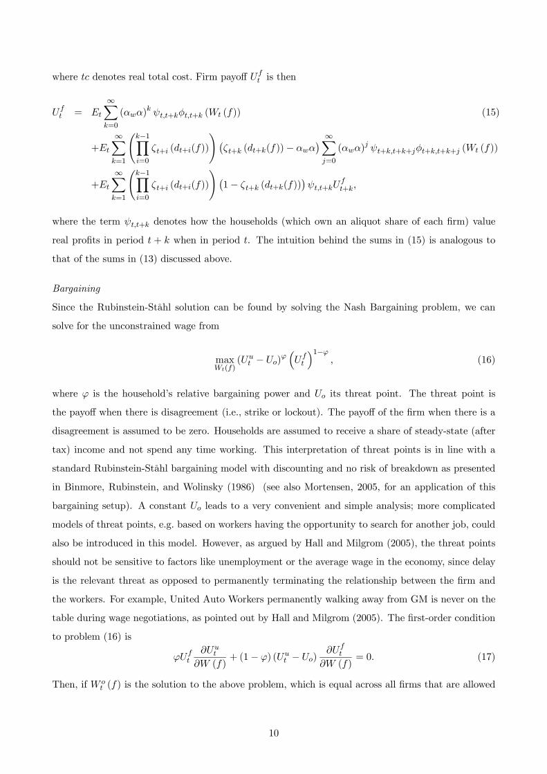
where tc denotes real total cost. Firm payoff Uft is then

Uft = Et

∞Xk=0

(αwα)k ψt,t+kφt,t+k (Wt (f)) (15)

+Et

∞Xk=1

Ãk−1Yi=0

ζt+i (dt+i(f))

!¡ζt+k (dt+k(f))− αwα

¢ ∞Xj=0

(αwα)j ψt+k,t+k+jφt+k,t+k+j (Wt (f))

+Et

∞Xk=1

Ãk−1Yi=0

ζt+i (dt+i(f))

!¡1− ζt+k (dt+k(f))

¢ψt,t+kU

ft+k,

where the term ψt,t+k denotes how the households (which own an aliquot share of each firm) value

real profits in period t + k when in period t. The intuition behind the sums in (15) is analogous to

that of the sums in (13) discussed above.

Bargaining

Since the Rubinstein-Ståhl solution can be found by solving the Nash Bargaining problem, we can

solve for the unconstrained wage from

maxWt(f)

(Uut − Uo)

ϕ³Uft

´1−ϕ, (16)

where ϕ is the household’s relative bargaining power and Uo its threat point. The threat point is

the payoff when there is disagreement (i.e., strike or lockout). The payoff of the firm when there is a

disagreement is assumed to be zero. Households are assumed to receive a share of steady-state (after

tax) income and not spend any time working. This interpretation of threat points is in line with a

standard Rubinstein-Ståhl bargaining model with discounting and no risk of breakdown as presented

in Binmore, Rubinstein, and Wolinsky (1986) (see also Mortensen, 2005, for an application of this

bargaining setup). A constant Uo leads to a very convenient and simple analysis; more complicated

models of threat points, e.g. based on workers having the opportunity to search for another job, could

also be introduced in this model. However, as argued by Hall and Milgrom (2005), the threat points

should not be sensitive to factors like unemployment or the average wage in the economy, since delay

is the relevant threat as opposed to permanently terminating the relationship between the firm and

the workers. For example, United Auto Workers permanently walking away from GM is never on the

table during wage negotiations, as pointed out by Hall and Milgrom (2005). The first-order condition

to problem (16) is

ϕUft

∂Uut

∂W (f)+ (1− ϕ) (Uu

t − Uo)∂Uf

t

∂W (f)= 0. (17)

Then, if W ot (f) is the solution to the above problem, which is equal across all firms that are allowed

10

to renegotiate, the resulting wage for firm f with the old contract Wt−1 (f) is

maxW ot (f) ,Wt−1 (f). (18)

Thus, in the case that the unconstrained optimal wage is lower than the present wage contract, the

old wage contract prevails due to the conflict cost structure outlined above.

As in price setting, we eliminate the distortions that result from bargaining. Since there are two

instruments that can be used to achieve this, i.e., τw and Uo, one of them is redundant. Here, we use

the method in Carlsson and Westermark (2006a), relying on adjusting τ and Uo to achieve efficiency.

1.3.1 Wage Evolution

Taking into account that firms cannot substitute across workers, the average wage is determined by

Wt = αw

Z 1

0Wt−1 (f) df + (1− αw)

ZWt−1(f)>W o

t (f)Wt−1 (f) df (19)

+(1− αw)

ZWt−1(f)≤W o

t (f)W o

t (f) df,

where the second term of (19) is due to downward nominal wage rigidity.

1.4 Steady State

As discussed above, downward nominal wage rigidity is not likely to have any noticeable real effects

in periods with high inflation rates. However, inflation rates have come down in most countries in

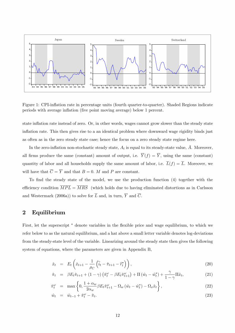
recent decades and prolonged periods of very low inflation rates are no longer uncommon. In figure

1, we plot the CPI-inflation rate (fourth quarter-to-quarter) for Japan, Sweden and Switzerland and

put a shade on low inflation periods, identified as quarters where the five-point moving average of CPI

inflation is below 1 percent. As can be seen in figure 1, lengthy periods where the maneuvering space

for adjusting real wages without reducing nominal wages is seriously limited is very much a real world

possibility.

To set ideas and capture the main mechanisms at work, we focus on a zero steady state inflation

regime in this paper. It is possible to allow for a (small) positive steady state inflation rate. However,

in order to retain tractability, we then need to index wages and prices that cannot be changed.13 But

indexation implies that welfare is independent of the steady state inflation rate. To see this, note that

indexation implies that the downward nominal rigidity will be centered around the positive steady

13 Indexation is needed since it is otherwise impossible to eliminate expectations of variables for more than one periodahead in the first-order conditions for wage and price setting. Thus, in the absence of indexation, it is necessary to keeptrack of infinite sums.

11

-2

-1

0

1

2

3

4

5

93 94 95 96 97 98 99 00 01 02 03 04 05

Switzerland

-2

-1

0

1

2

3

4

5

93 94 95 96 97 98 99 00 01 02 03 04 05

Japan

-2

-1

0

1

2

3

4

5

93 94 95 96 97 98 99 00 01 02 03 04 05

Sweden

Figure 1: CPI-inflation rate in percentage units (fourth quarter-to-quarter). Shaded Regions indicateperiods with average inflation (five point moving average) below 1 percent.

state inflation rate instead of zero. Or, in other words, wages cannot grow slower than the steady state

inflation rate. This then gives rise to a an identical problem where downward wage rigidity binds just

as often as in the zero steady state case; hence the focus on a zero steady state regime here.

In the zero-inflation non-stochastic steady state, At is equal to its steady-state value, A. Moreover,

all firms produce the same (constant) amount of output, i.e. Y (f) = Y , using the same (constant)

quantity of labor and all households supply the same amount of labor, i.e. L(f) = L. Moreover, we

will have that C = Y and that B = 0. M and P are constant.

To find the steady state of the model, we use the production function (4) together with the

efficiency condition MPL = MRS (which holds due to having eliminated distortions as in Carlsson

and Westermark (2006a)) to solve for L and, in turn, Y and C.

2 Equilibrium

First, let the superscript ∗ denote variables in the flexible price and wage equilibrium, to which we

refer below to as the natural equilibrium, and a hat above a small letter variable denotes log-deviations

from the steady-state level of the variable. Linearizing around the steady state then gives the following

system of equations, where the parameters are given in Appendix B,

xt = Et

µxt+1 −

1

ρC

³bit − πt+1 − br∗t´¶ , (20)

πt = βEtπt+1 + (1− γ)¡πωt − βEtπ

ωt+1

¢+Π (wt − w∗t ) +

γ

1− γΠxt, (21)

πωt = max

½0,1 + αw2αw

βEtπωt+1 −Ωw (wt − w∗t )−Ωxxt

¾, (22)

wt = wt−1 + πωt − πt. (23)

12

For clarity, all parameters are defined to be positive.

Equation (20) is a standard goods-demand (Euler) equation which relates the output gap xt, i.e.

the log-deviation between output and the natural output level, to the expected future output gap and

the expected real interest rate gap (bit − πt+1 − br∗t ), where bit denotes the log-deviation of the nominalinterest rate from steady state and br∗t is the log-deviation of the natural real interest rate from its

steady state.14 This relation is derived taking standard steps and using the households’ first-order

condition with respect to consumption, i.e., the consumption Euler equation.

The price-setting (Phillips) curve, equation (21), is derived using the firms’ first-order condition

(7), (see Carlsson and Westermark, 2006b, for details) and is similar in shape to the price-setting curve

derived by Erceg, Henderson, and Levin (2000), with the exception that current and expected future

wage inflation also enter the expression. Thus, price setting is affected by the real wage gap, i.e., the

log deviation between the real wage and the natural real wage (wt − w∗t ), the output gap xt, future

inflation Etπt+1 and current and future wage inflation πωt , Etπωt+1. As can be seen from Carlsson and

Westermark (2006b), the relevant real marginal cost measure driving inflation depends on the real wage

gap in firms that actually change prices (and, naturally, capital prices and productivity). However,

since we are interested in a price-setting relationship expressed in terms of the economywide real wage

gap, we need to adjust for the fact that interdependence in price and wage setting implies that the

economywide real wage gap and the real wage gap in firms that actually change prices are different in

our model.15 This motivates the “correction term” (1− γ)¡πωt − βEtπ

ωt+1

¢. Thus, in expression (21),

the real wage change in firms that change prices has been decomposed into the aggregate real wage

change wt and wage inflation terms πωt , Etπωt+1.

Equation (22) describes the wage setting behavior (see Appendix C and Carlsson and Westermark,

2006b, for details). From section (1.3) above, we know that wages are set according to (18). This

implies that wage inflation is non-negative and set according to the last term in the max operator

of (22) when positive. Hence, the max operator captures the restriction from wage setting in (22).

For positive wage inflation rates, wage inflation increases with higher expected wage inflation. The

coefficient in front of Etπωt+1, i.e.

1+αw2αw

β, is the probability adjusted discount rate from the wage

negotiations 1+αw2 β (where 1+αw

2 is the (unconditional) steady-state probability that wages remain

unchanged in the next period) multiplied by 1αw

, which governs how relative wages today (conditional

on πωt > 0) feed into wage-inflationary pressure. Moreover, as in Erceg, Henderson, and Levin (2000),

wage inflation is influenced by the real wage gap and the output gap. Since the parameters associated

14The nominal interest rate It is defined as the rate of return on an asset that pays one unit of currency under everystate of nature at time t+ 1.15Specifically, since all firms that are allowed to change wages are also allowed to change prices, the share of wage-

changing firms among the firms that change prices differs from the economywide average.

13

with these variables are determined by the bargaining problem, the size (and even the sign) of them

depend on e.g. the relative bargaining strength. See Carlsson and Westermark (2006a) for a detailed

discussion on wage setting in the unconstrained case.16

A caveat is in place here since the linearized wage-setting curve (22) is derived using the steady

state wage distribution. In general, since the last period’s wage is a state variable in today’s wage

setting problem, the aggregate wage outcome today will depend on the history of wage changes in the

economy, described by the wage distribution. However, starting from an initial distribution where all

firm/union pairs have the same wage, this will not be a problem when downward nominal wage rigidity

binds, since no one will reduce the wage anyway, although for periods beyond the first when wage

inflation is positive, the wage distribution potentially affects the aggregate wage inflation outcome.

We take this approach since it allows us to retain analytical tractability of the problem. Moreover, as

discussed above, this simplification should not lead us too far astray.

Finally, the evolution for the real wage (23) follows from the definition of the aggregate real wage

and states that today’s real wage is equal to yesterday’s real wage plus the difference between the

rates of wage and price change (πωt − πt).

As a comparison to the results from the economy with downward nominal wage rigidity, it is useful

to look at an economy where wages can adjust symmetrically. As shown in Carlsson and Westermark

(2006a), the unconstrained economy is described by (20), (21), (23) and replacing (22) with

πωt = βEtπωt+1 −Ωucw (wt − w∗t )−Ωucx xt (24)

where, once more, the parameter definitions are given in Appendix B.

3 The Monetary Policy Problem

The central bank is assumed to maximize social welfare. Here, we focus on the discretionary policy

case. Although studying optimal policy is in essence a normative enterprise, given that no central

bank formally commits to a policy rule it is natural to focus on the discretionary case. Following

the main part of the monetary policy literature, we focus on the limiting cashless economy (see e.g.

Woodford (2003) for a discussion) with the social welfare function

Et

∞Xt=0

βtµu (Ct)−

Z 1

0v (Lt (f)) df

¶. (25)

16See also Carlsson and Westermark (2006a), for a detailed comparison between the unconstrained version of (22), i.e.equation (24) below, and the wage setting curve resulting from the Erceg, Henderson, and Levin (2000) model.

14

Following Rotemberg and Woodford (1997), Erceg, Henderson, and Levin (2000), and others, we take

a second-order approximation to (25) around the steady state. This yields a standard expression for

the welfare gap (see Appendix C.5 for a detailed derivation, also c.f. Erceg, Henderson, and Levin

(2000)), i.e., the discounted sum of log-deviations of welfare from the natural (flexible price and wage

welfare level)

Et

∞Xt=0

βt³θx (xt)

2 + θπ (πt)2 + θπω (π

ωt )2´, (26)

where we have omitted higher order terms and terms independent of policy. As usual, θx < 0, θπ < 0

and θπω < 0 (see Appendix B for definitions). The first term captures the welfare loss (relative to

the flexible price and wage equilibrium) from output gap fluctuations stemming from the fact thatdmpl will differ from dmrs whenever xt 6= 0. However, even if xt = 0, there will be welfare losses due to

nominal rigidities. The reason is that nominal rigidities imply a non-degenerate distribution of prices

and wages. A non-degenerate distribution of prices and wages implies a non-degenerate distribution

of output across firms and working hours across households. This leads to welfare losses due to a

decreasing marginal product of labor and an increasing marginal disutility of labor.

Note that welfare only depends on variables xt, πt and πωt which, in turn, can solely be determined

from equations (21) to (23). To find the optimal rule under discretion, the central bank then solves

the following problem

V (wt−1, w∗t ) = max

xt,πt,πωt ,wtθx (xt)

2 + θπ (πt)2 + θπω (π

ωt )2 + βEtV

¡wt, w

∗t+1

¢, (27)

subject to equations (21) to (23), disregarding that expectations can be influenced by policy.

The wage inflation restriction (22) can be replaced by

πωt ≥ 1 + αw2αw

βEtπωt+1 −Ωxxt −Ωw (wt − w∗t )− πωt , (28)

πωt ≥ 0. (29)

Note that the problem with the original max constraint (23) and the problem with inequality

constraints (28) and (29) need not be equivalent. It is obviously true that a solution (xt, πt, πωt , wt) to

the problem with the original max constraint also satisfies the two inequality constraints. However, it

is possible that there is a solution (xt, πt, πωt , wt) to the problem with inequality constraints, so that

none of the inequality constraints is binding, thus leading to a violation of the original max constraint.

However, this is ruled out by the following Lemma.

Lemma 1 At least one of the inequality constraints (28) and (29) must be binding.

15

Proof : See Appendix D. ¥

Thus, this possibility is ruled out by the above Lemma, thereby implying that the problems are

equivalent. The intuition for the result is the following. Since the constraints (28) and (29) both put

lower bounds on πωt and, as can be seen from expression (26), welfare is decreasing in πωt , the central

bank sets πωt as low as possible, implying that one of the inequality constraints (28) and (29) must

bind.

From the above, it follows that the central banks’ problem (27) gives rise to two systems depending

on whether the inequality constraint binds. These systems, in turn, consist of the case specific first-

order conditions for optimal policy and restrictions from private sector behavior (see Appendix D for

details).

3.1 Numerical Solution and Calibration

To solve the model, we find the paths for xt, πt, πωt and wt that maximize welfare, as suggested by

Woodford (2003).17 ,18 As in Erceg, Henderson, and Levin (2000), we look at the effects of a technology

shock, which is assumed to follow an AR(1). It is straightforward to show that there is a positive

linear relationship between w∗t and At.19 Then, if technology follows an AR(1) process, w∗t also follows

an AR(1) process. We can thus model w∗t as

w∗t = ηw∗t−1 + εt, (30)

where εt is an (scaled) i.i.d. (technology) shock with standard deviation σ .

For our numerical exercises, we follow Erceg, Henderson, and Levin (2000), and assume that

u (Ct) =1

1− χC

¡Ct − Q

¢1−χC , (31)

and that

v (Lt) = −1

1− χL

¡1− Lt − Z

¢1−χn . (32)

Here, we introduce Q and Z in order to facilitate the comparison with Erceg, Henderson, and Levin

17We solve the problem in a different way than Erceg, Henderson, and Levin (2000), where an interest rate rule ispostulated and the parameters are chosen to maximize welfare.18To solve for the optimal instrument rule, the paths can be used together with the Euler equation and suitable criteria

for the shape of the rule; see Woodford (2003), for a discussion.19 It is possible to allow for other shocks. In the Technical Appendix of Carlsson and Westermark (2006a), we also

introduce a consumption shock and a labor-supply shock as in Erceg, Henderson, and Levin (2000). However, introducingthese shocks does not yield any additional insights here. In fact, it can easily be shown that under optimal policy, alldisturbances in the model (introduced as in Erceg, Henderson and Levin, 2000) can be reduced to a single disturbanceterm (being a linear combination of all these shocks).

16

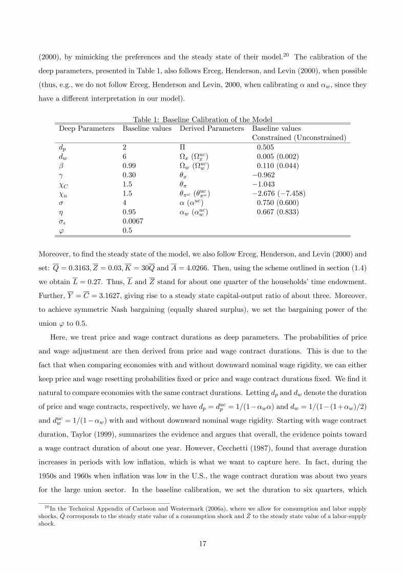
(2000), by mimicking the preferences and the steady state of their model.20 The calibration of the

deep parameters, presented in Table 1, also follows Erceg, Henderson, and Levin (2000), when possible

(thus, e.g., we do not follow Erceg, Henderson and Levin, 2000, when calibrating α and αw, since they

have a different interpretation in our model).

Table 1: Baseline Calibration of the ModelDeep Parameters Baseline values Derived Parameters Baseline values

Constrained (Unconstrained)dp 2 Π 0.505dw 6 Ωx (Ω

ucx ) 0.005 (0.002)

β 0.99 Ωw (Ωucw ) 0.110 (0.044)

γ 0.30 θx −0.962χC 1.5 θπ −1.043χn 1.5 θπω (θ

ucπω) −2.676 (−7.458)

σ 4 α (αuc) 0.750 (0.600)η 0.95 αw (αucw ) 0.667 (0.833)σ 0.0067ϕ 0.5

Moreover, to find the steady state of the model, we also follow Erceg, Henderson, and Levin (2000) and

set: Q = 0.3163, Z = 0.03,K = 30Q and A = 4.0266. Then, using the scheme outlined in section (1.4)

we obtain L = 0.27. Thus, L and Z stand for about one quarter of the households’ time endowment.

Further, Y = C = 3.1627, giving rise to a steady state capital-output ratio of about three. Moreover,

to achieve symmetric Nash bargaining (equally shared surplus), we set the bargaining power of the

union ϕ to 0.5.

Here, we treat price and wage contract durations as deep parameters. The probabilities of price

and wage adjustment are then derived from price and wage contract durations. This is due to the

fact that when comparing economies with and without downward nominal wage rigidity, we can either

keep price and wage resetting probabilities fixed or price and wage contract durations fixed. We find it

natural to compare economies with the same contract durations. Letting dp and dw denote the duration

of price and wage contracts, respectively, we have dp = ducp = 1/(1−αwα) and dw = 1/(1−(1+αw)/2)

and ducw = 1/(1−αw) with and without downward nominal wage rigidity. Starting with wage contract

duration, Taylor (1999), summarizes the evidence and argues that overall, the evidence points toward

a wage contract duration of about one year. However, Cecchetti (1987), found that average duration

increases in periods with low inflation, which is what we want to capture here. In fact, during the

1950s and 1960s when inflation was low in the U.S., the wage contract duration was about two years

for the large union sector. In the baseline calibration, we set the duration to six quarters, which

20 In the Technical Appendix of Carlsson and Westermark (2006a), where we allow for consumption and labor supplyshocks, Q corresponds to the steady state value of a consumption shock and Z to the steady state value of a labor-supplyshock.

17

is higher than suggested by Taylor (1999), but still being conservative relative to the low inflation

estimate from Cecchetti (1987).

For price contract duration, the micro evidence presented by Bils and Klenow (2004), suggests a

price duration of about five months, whereas the micro evidence presented by Nakamura and Steinsson

(2007), and the survey evidence in Blinder, Canetti, Lebow, and Rudd (1998), suggest about eight

months. In our baseline calibration, we set the price duration to two quarters which is in the range

given by the above studies.

Then, using the steady state solution together with the definitions for the derived parameters

(presented in appendix A) yields the values presented in Table 1.

It is interesting to see the high coefficient for wage inflation variance in the loss function (θπω).

Starting with the constrained case, we see that the coefficient on wage inflation variance (θπω) is about

three times larger than the coefficient on the variance in the output gap (θx) and the coefficient on

the variance in inflation (θπ). Thus, variation in wage inflation is associated with considerable welfare

losses. Moreover, when relaxing the downward nominal wage rigidity constraint, the coefficient on

wage inflation almost triples in size relative to the constrained economy. The reason is that since

wages never fall in the constrained economy there will be a cap on the relative wage misalignment

that a given wage inflation gives rise to.

To obtain a ball-park estimate of σ , we make use of a the Taylor (1993) rule estimated by

Rudebusch (2002) (see expression (33) below) as an approximation of actual monetary policy and

impose it on the unconstrained version of the model. Then, we set σ to match the standard deviation

of quarterly inflation in the model with the actual standard deviation of the U.S. quarterly CPI inflation

(1987:Q4-1999:Q4).21 This results in a standard deviation of the innovation to the w∗t process of 0.0067

(= σ ).

Numerically, we solve the model by iterating on the policy functions and updating the value

function given the new policy functions. In the procedure, we also take into account how expectations

in the constraints are affected by this (see (121) in Appendix D).

A standard reference for algorithms with occasionally binding constraints is Christiano and Fisher

(2000). Unfortunately, we cannot use this algorithm since our model is slightly different. Specifically,

our problem includes expectations of the control variables in the constraints. The way in which we

take care of this problem is to use that the control variables are functions of the state variables (i.e.,

the policy functions) and rewrite the constraint set in terms of state variables only.22 This is related

21We focus on inflation for the calibration, since this is the only variable we can directly observe without resorting tosome filtering technique.22Note that policy functions are potentially nonlinear, since there is a non-linear constraint to the problem (i.e.

constraint (22)).

18

to the method used in e.g., Soderlind (1999). However, instead of using the policy functions from

the previous iteration as is done in Soderlind (1999), we use the current policy functions, as in the

algorithm used in e.g., Krusell, Quadrini, and Rios-Rull (1996). Note that the algorithm in Krusell,

Quadrini, and Rios-Rull (1996) can be considered as analyzing a one-period deviation from a proposed

policy. Iteration finishes when there are no gains from deviating from the proposed policy. The full

algorithm is outlined in appendix A.

4 Optimal Policy V.S. Simple Rules

First, we solve the model for the calibration described above, both in the case with and without

downward nominal wage rigidity under optimal discretionary monetary policy. In figure 2, we plot

the impulse responses to a one standard deviation negative shock to the natural real wage w∗t .

0 5 10 15 20−0.03

−0.025

−0.02

−0.015

−0.01

−0.005

0

0.005Output gap

Time0 5 10 15 20

−0.05

0

0.05

0.1

0.15

0.2

0.25

0.3

Inflation

Time

Optimal Discretionary Policy ConstrainedOptimal Discretionary Policy Unconstrained

0 5 10 15 20−0.04

−0.02

0

0.02

0.04

0.06

0.08Wage Inflation

Time0 5 10 15 20

−0.55

−0.5

−0.45

−0.4

−0.35

−0.3

−0.25

−0.2Real Wage

Time

Figure 2: Impulse responses to a one standard deviation negative shock in the natural real wage. Scalecorresponds to percentage units.

Starting with the unconstrained case, the negative shock drives down the natural real wage implying

that the actual real wage is higher than the natural real wage, thus initially causing a positive real-wage

gap. The real wage can be adjusted by changing inflation and wage inflation. Holding the inflation

rate above the wage inflation rate decreases the real wage. However, since it is costly to stabilize the

real wage gap, in terms of the implied variation in inflation, wage inflation and the output gap, it is

optimal not to fully compensate for the shock. For the same reason, optimality requires that inflation

and wage inflation should be kept (approximately) at opposite sides of zero (the path of xt must also

19

be considered). Thus, the optimal initial inflation response is positive, whereas the wage inflation

response is negative. But the difference between them is not sufficiently large to immediately fully

close the real-wage gap.

Given the AR(1) structure of the shock, the natural real wage increases towards the steady value

of zero after the initial negative shock. So at some point, the central bank needs to start increasing the

real wage in order to continue to stabilize the economy. This is also what we see after approximately

four quarters. For this purpose, the relationship between inflation and wage inflation needs to be

reversed, which also happens at this point in time.

In the constrained case, wage inflation cannot be used to initially lower the real wage. Instead,

optimal policy prescribes a stronger initial inflation reaction relative to the unconstrained case, and

also allow for a larger output gap in order to stabilize the real-wage gap. However, the initial optimal

inflation response is not sufficient to stabilize the real wage gap to the same extent as in the uncon-

strained case. This is reflected by the initial real wage response in the constrained case lying above

the real wage response in the unconstrained case.

In figure 3, we plot the resulting impulse responses to a one standard deviation positive shock to

w∗t . For the unconstrained case, the impulse responses are a mirror image through the horizontal

0 5 10 15 20−0.005

0

0.005

0.01

0.015

0.02

0.025

0.03Output gap

Time0 5 10 15 20

−0.3

−0.25

−0.2

−0.15

−0.1

−0.05

0

0.05Inflation

Time

Optimal Discretionary Policy ConstrainedOptimal Discretionary Policy Unconstrained

0 5 10 15 20−0.04

−0.02

0

0.02

0.04

0.06

0.08Wage Inflation

Time0 5 10 15 20

0.2

0.3

0.4

0.5

Real Wage

Time

Figure 3: Impulse responses to a one standard deviation positive shock in the natural real wage. Thescale corresponds to percentage units.

axis of the negative case. We now see that the initial optimal inflation and output gap responses are

smaller than in the unconstrained case. However, the initial wage inflation response is larger than

20

in the unconstrained case. Note that downward nominal wage rigidity does not only affect private

sector behavior but also the parameters in the loss function in making the parameter for wage inflation

smaller. Below we will decompose the effects on welfare from the change in the loss function from the

effects stemming from changes in private sector behavior. However, any asymmetry in the impulse

response paths across positive and negative shocks must stem from private sector behavior and not

from the (symmetric) loss function.

In figure 4, we plot the optimal interest rate path (in terms of deviations from steady state) for

the unconstrained and constrained case, respectively. As can be seen in figure 4, the optimal interest

0 5 10 15 20

0

0.05

0.1

0.15

0.2

Interest Rate Response (Negative Shock)

Time0 5 10 15 20

−0.2

−0.15

−0.1

−0.05

0

Interest Rate Response (Positive Shock)

Time

Optimal Discretionary Policy ConstrainedOptimal Discretionary Policy Unconstrained

Figure 4: Optimal interest-rate responses to a one standard deviation positive and negative shock inthe natural real wage. The scale corresponds to percentage units.

rate response is asymmetric in the constrained case. Especially, the interest rate response is larger in

the constrained case for negative shocks and smaller for positive shocks relative to the unconstrained

case.

Next, we turn to welfare analysis. Note first that it need not be the case that the model with

the downward nominal wage rigidity constraint necessarily leads to lower welfare relative to the un-

constrained case. The reason is that this is not just an additional constraint on the problem, i.e., a

constraint that makes the feasible set smaller. Instead, it is a constraint that changes the choice set.23

Also, another factor is that the parameter on wage inflation variance in the welfare function changes

23To see this, consider the relationship between, say πω and x in equation (22), treating other variables as constants.Then, in the unconstrained case, the relationship is linear with slope Ωx. In contrast, in the constrained case, therelationship is piecewise linear with zero slope below some critical value of x and with slope Ωx above this value.

21

when imposing downward nominal wage rigidity. Thus, overall, the welfare effect from downward

nominal wage rigidity is ambiguous a priori.

To compute welfare, we construct sequences of shocks for 1000 periods and use these to find paths

for the variables xt, πt, πωt and wt. Then, welfare is computed from these paths using the welfare

criterion (26), ignoring the periods t > 1000. This is repeated 1000 times to generate an approximation

of the expectation. Finally, to express the welfare loss as a fraction of steady state consumption, we

scale the welfare difference (26) by 1/¡uC¡C, Q

¢C¢.

In the unconstrained case, we find a welfare difference relative to the natural (flexible price and

wage) welfare level of 0.186 percentage units of steady state consumption. Interestingly, the result

for the constrained case is almost identical with a difference of 0.181. Thus, downward nominal wage

rigidity does not necessarily lead to large welfare losses, as is often considered. In fact, in our model we

find a (very) modest welfare gain. Now, since introducing downward nominal wage rigidity does not

only affect the behavior of the private sector, but also the parameter in the loss function on variation

in wage inflation (c.f. Table 1 above), it is interesting to try to isolate the effects. To this end, we both

solve for the unconstrained optimal policy, as well as calculate the welfare loss using the parameters

for the loss function from the constrained case. The resulting welfare difference is 0.178, which is

very close to the original results for the unconstrained case (0.186). Thus, the similarity between

the welfare outcomes in the unconstrained and constrained cases is not driven by the increase in the

loss-function parameter on wage inflation variance.

The intuition for the small welfare effects is that downward nominal wage rigidity is not all that

harmful since it may help keep down wage dispersion (see below). This, in turn, can be exploited by

the central bank when designing optimal monetary policy.

A Simple Rule

Next, we turn to analyzing the effects on welfare from relying on a simple instrument rule instead of

the optimal policy rule. To this end, we impose a Taylor (1993) rule, i.e.

bit = 1.24πt + 0.33xt, (33)

where the parameters for (33) are calibrated to match the estimates in Rudebusch (2002). Note

that this rule does not take any asymmetry into account when setting the interest rate, although the

economy will react asymmetrically to positive and negative shocks, due to private sector behavior.24

24To implement the Taylor rule, we replace the central bank’s first-order condition in systems (135) and (139) inAppendix C with the sticky price Euler equation (20), where we have used the corresponding flexible-price Euler equationto eliminate the real natural interest rate and the Taylor rule to eliminate the nominal interest rate. For the system

22

In figure 5, we plot the resulting impulse responses to a one standard deviation negative shock to

w∗t when the nominal interest rate is governed by a Taylor rule as well as under optimal policy.

0 5 10 15 20

−0.1

−0.05

0

0.05

0.1

0.15Output gap

Time0 5 10 15 20

−0.05

0

0.05

0.1

0.15

0.2

0.25

0.3

Inflation

Time

Optimal Discretionary Policy ConstrainedTaylor Rule Constrained

0 5 10 15 20

0

0.02

0.04

0.06

0.08

0.1Wage Inflation

Time0 5 10 15 20

−0.55

−0.5

−0.45

−0.4

−0.35

−0.3

−0.25

−0.2Real Wage

Time

Figure 5: Impulse responses to a one standard deviation negative shock to w∗t when the nominalinterest rate is governed by a Taylor rule as well as under the optimal policy. Scale corresponds topercentage units.

Note that the impulse responses are not smooth as under optimal policy. The reason for this is that

the Taylor rule is not optimally chosen and has the same functional form for both the case when

downward nominal wage rigidity binds and when it does not. Interestingly, the Taylor rule responses

for inflation are in fact fairly similar to the optimal responses. However, for wage inflation, the Taylor

rule undershoots slightly when the constraint stops binding, all in all leading to substantial excess

volatility in the output gap. In figure 6, we plot the resulting impulse responses to a one standard

deviation positive shock to w∗t . Once more, the Taylor rule responses for inflation are similar to the

optimal responses. However, the initial wage inflation response now overshoots. Once more, the

volatility in the output gap is substantially larger than in the optimal responses. 25

Next we turn to welfare. Note that it is not a trivial result that optimal discretionary policy

outperforms the Taylor rule, since the Taylor rule is, in fact, a commitment rule and hence, could

perform better than the optimal discretionary rule. However, we do find that optimal discretionary

under the Taylor rule, there is no need to iterate on the value function. Instead, we can directly solve the system for thepolicy functions (i.e. we only do step 1 in the numerical algorithm outlined in Appendix A). Then, we can simulate themodel and evaluate welfare as done above.25 For brevity, we do not plot interest rate responses, since they are mainly a reflection of differences in the output

gap responses.

23

0 5 10 15 20

−0.1

−0.05

0

0.05

0.1

0.15Output gap

Time0 5 10 15 20

−0.3

−0.25

−0.2

−0.15

−0.1

−0.05

0

0.05Inflation

Time

Optimal Discretionary Policy ConstrainedTaylor Rule Constrained

0 5 10 15 20

0

0.02

0.04

0.06

0.08

0.1Wage Inflation

Time0 5 10 15 20

0.2

0.3

0.4

0.5

Real Wage

Time

Figure 6: Impulse responses to a one standard deviation positive shock to w∗t when the nominalinterest rate is governed by a Taylor rule as well as under the optimal policy. Scale corresponds topercentage units.

policy performs better than the policy prescribed by the Taylor rule. In terms of steady state con-

sumption, the additional loss is about 0.07 percentage units of steady state consumption. But, all in

all, the Taylor rule seems to be a fairly good approximation of optimal discretionary monetary policy

in the presence of downward nominal wage rigidity.

Finally, we look at the impulse responses for the unconstrained economy versus an economy with

downward nominal wage rigidity under the Taylor rule. In figure 7, we plot the resulting impulse

responses to a one standard deviation negative shock to w∗t . The key result here is that downward

nominal wage rigidity actually helps stabilize the economy in the wage inflation dimension, whereas it

does not induce much more variation in inflation and the output gap. A fairly similar result appears

from figure 8, where we plot the resulting impulse responses to a one standard deviation negative

shock to w∗t . Most notably, the wage inflation variability is not substantially larger in the downward

rigid case. This is also the dimensions about which the households care most (c.f. table 1).

When looking at welfare differences, we find that welfare loss is quite a bit lower in the economy

with downward nominal wage rigidity relative to the unconstrained economy when monetary policy

is governed by the Taylor rule. In terms of steady state consumption, the welfare gain is about 0.14

percentage units of steady state consumption. Thus, an agent would in this case prefer an economy

with downward nominal wage rigidity over an economy with downward nominal wage flexibility ex ante.

24

0 5 10 15 20

−0.1

−0.05

0

0.05

0.1

0.15Output gap

Time0 5 10 15 20

−0.05

0

0.05

0.1

0.15

0.2

0.25

0.3

Inflation

Time

Taylor Rule UnconstrainedTaylor Rule Constrained

0 5 10 15 20−0.05

0

0.05

0.1Wage Inflation

Time0 5 10 15 20

−0.55

−0.5

−0.45

−0.4

−0.35

−0.3

−0.25

−0.2Real Wage

Time

Figure 7: Impulse responses to a one standard deviation negative shock to w∗t when the nominalinterest rate is governed by a Taylor rule. Scale corresponds to percentage units.

0 5 10 15 20

−0.1

−0.05

0

0.05

0.1

0.15Output gap

Time0 5 10 15 20

−0.3

−0.25

−0.2

−0.15

−0.1

−0.05

0

0.05Inflation

Time

Taylor Rule UnconstrainedTaylor Rule Constrained

0 5 10 15 20−0.05

0

0.05

0.1Wage Inflation

Time0 5 10 15 20

0.2

0.3

0.4

0.5

Real Wage

Time

Figure 8: Impulse responses to a one standard deviation positive shock to w∗t when the nominalinterest rate is governed by a Taylor rule. Scale corresponds to percentag units.

25

Evaluating the unconstrained economy with the loss function of the constrained economy suggests a

welfare gain from downward nominal wage rigidity of about 0.08 percent of steady state consumption.

Thus, once more, the above result is not just driven by the increase in the loss-function parameter on

wage inflation, when relaxing the constraint while keeping the duration of price and wage contracts

constant. Instead, private sector behavior plays an important part in explaining the results.

Wage-Inflation Distributions and Welfare

To see the consequences for welfare, we illustrate the wage-inflation distributions in four histograms;

see figure 9. First, if we vary policy, i.e., compare the Taylor rule and optimal policy, the distribution

−0.4 −0.2 0 0.2 0.4

Optimal Policy Unconstrained

−0.4 −0.2 0 0.2 0.4

Optimal Policy Constrained

−0.4 −0.2 0 0.2 0.4

Emprical Taylor Rule

−0.4 −0.2 0 0.2 0.4

Empirical Taylor Rule Constrained

Figure 9: Histograms of simulated wage-inflation paths.

is more dispersed under the Taylor rule. This seems to hold irrespectively whether there are downward

nominal wage rigidities or not. If we fix the policy regime, on the other hand, the distribution seems

to have lower variability with downward nominal wage rigidities than without.

4.1 Robustness

A key parameter for welfare evaluation is the standard deviation of the innovation to w∗t , σ . We now

consider increasing σ by 50 percent. The results of this experiment are presented in Table 2. We see

that this does not change the qualitative conclusions from our baseline simulation, in terms of welfare

rankings. But increasing the shock size does increase the welfare loss in all four cases.

26

Table 2: Robustness - Shock SizeWelfare Differences Relative to Flex Price

Baseline (σ = 0.0067) Big Shocks (σ = 0.0101)Unc. Opt. −0.1856 −0.4176Con. Opt. −0.1809 −0.4125Unc. Taylor −0.3872 −0.8723Con. Taylor −0.2508 −0.6118The values are expressed in terms of percentage units of steady state consumption.

In the baseline calibration, the wage-contract duration is six quarters. Since this may seem to

be on the high side (even though it is in line with the evidence of wage-contract durations in low-

inflation environments), we also see to what extent our results are robust to varying the wage-contract

duration. In table 3, we present the results from decreasing the wage duration by a quarter. As can

be seen in the table, decreasing the duration of the wage contracts leads to slightly smaller welfare

Table 3: Robustness - Contract DurationsWelfare Differences Relative to Flex Price

Contract Durations dp = 2, dw = 6 dp = 2, dw = 5

Unc. Opt. −0.1856 −0.1759Con. Opt. −0.1809 −0.1761Unc. Taylor −0.3872 −0.3767Con. Taylor −0.2508 −0.2436The values are expressed in terms of percentage units of steady state consumption.

losses in all cases. Also, note that the welfare ranking between the optimal policy in the constrained

and unconstrained case shifts to a tiny advantage for the unconstrained case. However, the key point

that downward nominal wage rigidity does not imply large welfare losses is robust.

Finally, we have also experimented to see how sensitive the results are to the exact values of the

parameters in the Taylor rule. In table 4, we present the result from using the original values from

Taylor (1993) (i.e., βπ = 1.5 and βx = 0.5). When using the Taylor (1993) parameter values for

Table 4: Robustness - Taylor Rule ParametersWelfare Differences Relative to Flex Price

Taylor Rule βπ = 1.24, βx = 0.33 βπ = 1.5, βx = 0.5

Unc. Taylor −0.3872 −0.3224Con. Taylor −0.2508 −0.2604

The values are expressed in terms of percentage units of steady state consumption.

the Taylor rule, the welfare loss decreases without downward nominal wage rigidity, while the welfare

loss almost remains unchanged when downward nominal wage rigidities are present. Thus, the results

indicate that downward nominal wage rigidity makes the welfare outcome less sensitive to the exact

calibration of the Taylor rule.

27

Overall, the key points from the previous section seem to be robust.

5 Concluding remarks

In this paper, we study the implications for optimal monetary policy when declining nominal wages

do not constitute a viable margin for adjustment to adverse economic conditions. To this end, a

New Keynesian model is developed that can endogenously account for downward nominal wage rigid-

ity. This is achieved by introducing wage bargaining between firms and unions in the model as in

Holden (1994). Under asymmetric conflict costs, downward nominal wage rigidity arises as a rational

endogenous outcome.

Focusing on optimal discretionary monetary policy, we show that when money wages cannot fall,

the optimal policy response to changing economic conditions becomes asymmetric. More specifically,

inflation and the output gap respond more when the downward nominal wage rigidity constraint binds.

Interestingly, in our baseline case the welfare loss is actually slightly smaller in an economy with

downward nominal wage rigidities. The reason is that downward nominal rigidity is not an additional

constraint on the problem. Instead, it is a constraint that changes the choice set and opens up for

potential welfare gains. Another effect of downward nominal wage rigidity is that the loss function

parameter for wage inflation variation is changed, although this latter effect seems to play a small

role in explaining the welfare effects of downward nominal wage rigidity (at least under optimal

policy). We also find that the Taylor rule estimated by Rudebusch (2002), provides a fairly good

approximation of optimal discretionary policy in terms of welfare under downward nominal wage

rigidity. Experimenting with using the original Taylor (1993), parameters for the Taylor rule indicates

that the exact specification of the Taylor rule actually plays a minor role for this property. In contrast,

the Taylor rule does not provide such a good approximation of optimal policy in the unconstrained case.

A corollary then is that, under the Taylor rule, agents would clearly prefer an economy with downward

nominal wage rigidities rather than an unconstrained economy ex ante. That is, since downward

nominal wage rigidity actually helps stabilizing the economy in the wage inflation dimension and

hence, reduces wage variability, but does not induce much more variation in inflation and the output

gap.

28

References

Agell, J., and P. Lundborg (2003): “Survey Evidence on Wage Rigidity and Unemployment:

Sweden in the 1990s,” Scandinavian Journal of Economics, 105, 15—29.

Akerlof, G., W. T. Dickens, and G. Perry (1996): “The Macroeconomics of Low Inflation,”

Brookings Papers on Economic Activity, (1).

Altissimo, F., M. Ehrmann, and F. Smets (2006): “Inflation persistence and price-setting in the

Euro Area,” ECB Occasional Paper Series No. 46.

Altonji, J., and P. Devereux (2000): “The Extent and Consequences of Downward Nominal Wage

Rigidity,” in Research in Labor Economics, ed. by S. Polachek, vol. 19, pp. 383—431. Elsevier.

Baker, G., M. Gibbs, and B. Holmstrom (1994): “The Wage Policy of a Firm,” Quarterly Journal

of Economics, 109, 921—955.

Barro, R., and D. Gordon (1983a): “A Positive Theory of Monetary Policy in a Natural Rate

Model,” Journal of Political Economy, 91, 589—610.

(1983b): “Rules, Discretion and Reputation in a Model of Monetary Policy,” Journal of

Monetary Economics, 12, 101—121.

Bewley, T. (1999): Why Wages Don’t Fall During a Recession. Harvard University Press, Cam-

bridge, MA.

Bils, M., and P. Klenow (2004): “Some Evidence on the Importance of Sticky Prices,” Journal of

Political Economy, 112, 947—985.

Binmore, K., A. Rubinstein, and A. Wolinsky (1986): “The Nash Bargaining Solution in Eco-

nomic Modelling,” RAND Journal of Economics, 17, 176—188.

Blinder, A., E. Canetti, D. Lebow, and J. Rudd (1998): Asking About Prices: A New Approach

to Understand Price Stickiness. Russel Sage Foundation, New York.

Calvo, G. (1983): “Staggered Prices in a Utility-Maximizing Framework,” Journal of Monetary

Economics, 12, 383—398.

Carlsson, M., and A. Westermark (2006a): “Monetary Policy and Staggered Wage Bargaining

when Prices are Sticky, Sveriges Riksbank Working Paper No. 199,” .

(2006b): “Technical Appendix to Monetary Policy and Staggered Wage Bargaining when

Prices are Sticky, mimeo, Sveriges Riksbank,” .

Cecchetti, S. (1987): “Indexation and Incomes Policy: A Study of Wage Adjustments in Unionized

Manufacturing,” Journal of Labor Economics, 5, 391—412.

29

Christiano, L., and J. Fisher (2000): “Algorithms for solving dynamic models with occasionally

binding constraints,” Journal of Economic Dynamics and Control, 24, 1179—1232.

Dickens, W., L. Goette, E. Groshen, S. Holden, J. Messina, M. Schweitzer, J. Turunen,

and M. Ward (2006): “How Wages Change: Micro Evidence from the International Wage

Flexibility Project, ECB Working Paper Series No. 697,” .

Erceg, C., D. Henderson, and A. Levin (2000): “Optimal Monetary Policy with Staggered Wage

and Price Contracts,” Journal of Monetary Economics, 46, 281—313.

Fehr, E., and L. Goette (2005): “Robustness and Real Consequences of Nominal Wage Rigidity,”

Journal of Monetary Economics, 52, 779—804.

Gordon, R. (1996): “Comment and Discussion: Akerlof et al.: The Macroeconomics of Low Infla-

tion.,” Brookings Papers on Economic Activity, pp. 60—76.

Hall, R., and P. Milgrom (2005): “The Limited Influence of Unemployment on the Wage Bargain,”

NBER Working Paper No. 11245.

Holden, S. (1994): “Wage Bargaining and Nominal Rigidities,” European Economic Review, 38,

1021—1039.

Holden, S., and F. Wulfsberg (2007): “Downward Nominal Wage Rigidity in the OECD, mimeo,

University of Oslo,” .

Judd, K. L. (1998): Numerical Methods in Economics. MIT Press, Cambridge, MA.

Krusell, P., V. Quadrini, and J.-V. Rios-Rull (1996): “Are consumption taxes really better

than income taxes,” Journal of Monetary Economics, 37, 475—503.

Kuroda, S., and I. Yamamoto (2003a): “Are Japanese Nominal Wages Downwardly Rigid? (Part

I): Examinations of Nominal Wage Change Distributions,” Monetary and Economic Studies,

21(2), 1—30.

(2003b): “Are Japanese Nominal Wages Downwardly Rigid? (Part II): Examinations Using

a Friction Model,” Monetary and Economic Studies, 21(2), 31—68.

Mortensen, D. (2005): “Growth, Unemployment, and Labor Market Policy,” Journal of the Euro-

pean Economic Association, 3, 236—258.

Nakamura, E., and J. Steinsson (2007): “Five Facts About Prices: A Reevaluation of Menu Cost

Models,” mimeo Harvard University.

Rotemberg, J., and M. Woodford (1997): “An Optimization-Based Econometric Framework for

the Evaluation of Monetary policy,” in NBER Macroeconomics Annual, ed. by B. Bernanke, and

J. Rotemberg. MIT Press, Cambridge, MA.

30

Rubinstein, A. (1982): “Perfect Equilibrium in a Bargaining Model,” Econometrica, 50, 97—109.

Rudebusch, G. (2002): “Term Structure Evidence on Interest Rate Smoothing and Monetary Policy

Inertia,” Journal of Monetary Economics, 49, 1161—1187.

Soderlind, P. (1999): “Solution and estimation of RE macromodels with optimal policy,” European

Economic Review, 43, 813—823.

Taylor, J. (1993): “Discretion Versus Policy Rules in Practice,” Carnegie-Rochester Conference

Series on Public Policy, 39, 195—214.

(1999): “Staggered Price and Wage Setting in Macroeconomics,” in Handbook of Macroeco-

nomics, ed. by J. Taylor, and M. Woodford, vol. 1B. Elsevier, Amsterdam.

Wilson, B. A. (1999): “Wage Rigidity: A Look Inside the Firm,” Mimeo, Federal Reserve Board of

Governors.

Woodford, M. (2003): Interest and Prices: Foundations of a Theory of Monetary Policy. Princeton

University Press, Princeton, NJ.

31

Appendix

A Numerical Algorithm

The main outline of the algorithm follows algorithm 12.2 in Judd (1998). We first define N ⊂ R2

nodes over the state space.

Step 0. Guess policy functions U0i , i.e., parameter values in second-order complete polynomials

π0 (wt−1, w∗t ) ,

πω0 (wt−1, w∗t ) , (34)

x0 (wt−1, w∗t ) ,

and value function

V 0 (wt−1, w∗t ) . (35)

Then proceed to step 2.

Step 1. Consider systems (135) and (139) derived by using the first three first-order conditions in

(130) to eliminate the Lagrange multipliers in the last first-order condition, together with the three

constraints (21) to (23) (see the discussion in section 4 and Appendix C) We find the new guess

for the policy functions U l+1i by solving for these from systems (135) and (139), respectively, with a

collocation method. While solving for policy functions, we take into account that the policy functions

affect the expectations.

Step 2. Compute current period utility P l+1i for i = 1, . . . , N , given policy function guesses U l+1

i .26

Step 3. Update the value function V l+1 (wt−1, w∗t ) using

V l+1 =³I − βQU l+1

´−1P l+1, (36)

where QU l+1is the transition matrix defined by the new guess for the policy functions for inflation

and wage inflation and the flow equation for real wages.

Step 4. If°°V l+1 − V l

°° < ε stop. Otherwise, go to step 1.

B Parameter Definitions

The parameters in the equilibrium relations are defined as

26 In terms of Judd (1998) p. 416, compute π yi, Ul+1i where U l+1

i consists of πt, πωt and xt and yi = (wt−1, w∗t )i,

which gives P l+1i = π yi, U

l+1i .

32

Ωx = Π1ΦxΦd, Ωucx = Πuc1

ΦxΦd,

Ωw = Π1ΦwΦd

, Ωucw = Πuc1ΦwΦd

,(37)

where

Π1 =¡1− 1+αw

2 β¢1−αwαw

, Πuc1 = (1− αwβ)1−αwαw

,

Π = 1−αwααwα

(1− αwαβ) ,(38)

and Φx, Φw and Φd are defined as (see the Appendix C below for details)

Φd = εL1

σ − 1 (ϕ (2 + (1 + ρL) εL)− (1 + εL)) vLL− ϕvLL

1− γ(1− γ)2 (39)

Φx =

µ−ϕ εL

σ − 1

µρC − ρL

1− σγ

1− γ

¶− (1− ϕ)σγ

¶vLL+ ϕ

1

σ − 1vLL

1− γ(1− σγ − ρC (1− γ))

Φw = −µ−ϕ εL

σ − 1 (1− σρL) + (1− ϕ) (1− γ)σ

¶vLL+ ϕ

1

σ − 1vLL

1− γ(1 + εL)

where

εL = − (γ + σ (1− γ)) . (40)

Let

ρC = −uCCC

uC= χC

C

C − Qand ρL = −

vLLL

vL= −χn

L

1− L− Z. (41)

The loss function parameters in (26) are then defined as

θx =C

2uC

µ−ρC + ρL

1

1− γ− γ

1− γ

¶,

θπ = − vLL2

σ (γ (1− σ) + 1 + γ)

1− γ

1

Π, (42)

θπω = − vLL2

µ−γεL + (1− γ)σ (1 + γ (1− σ))

Π1− (1− γ)

σ (γ (1− σ) + 1 + γ)

Π

¶.

and for the unconstrained case we need to replace θπω with θucπω defined as

θucπω = −vLL

2

µ−γεL + (1− γ)σ (1 + γ (1− σ))

Πuc1− (1− γ)

σ (γ (1− σ) + 1 + γ)

Π

¶. (43)

33

C Some Derivations

Most of the derivations in the paper are similar to those in Carlsson and Westermark (2006b). Here,

we present the derivations that must be modified due to downward nominal wage rigidity. Thus, the

changes concern the sections where wage setting is a part. Hence, wage setting itself must be modified,

as well as part of the steady state analysis and the welfare computations.

C.1 Wages

As in Carlsson and Westermark (2006b), we use gradient notation (∇) to indicate derivatives. We can

write the derivative of U tu as

∇WU tu = Et

∞Xk=0

(αwαβ)k∇WΥt,t+k +Et

∞Xk=1

k−1Yi=0

ζt+i (dt+i)¡ζt+k (dt+k)− αwα

¢βk

×∞Xj=0

(αwαβ)j∇WΥt+k,t+k+j +Et

∞Xk=1

k−1Xi=1

⎛⎜⎝ k−1Ym=0m6=i

ζt+m (dt+m)

⎞⎟⎠ (1− αw)∇W ζt+i (dt+i)

×

⎛⎝¡ζt+k (dt+k)− αwα¢βk

∞Xj=0

(αwαβ)j Υt+k,t+k+j +

¡1− ζt+k (dt+k)

¢βkU t+k

u

⎞⎠ (44)

+Et

∞Xk=1

Ãk−1Yi=0

ζt+i (dt+i)

!∇W ζt+k (dt+k)β

k

⎛⎝ ∞Xj=0

(αwαβ)j Υt+k,t+k+j − U t+k

u

⎞⎠and the derivative of U t

f as

∇WU tf = Et

∞Xk=0

(αwα)k ψt,t+k∇Wφt,t+k +Et

∞Xk=1

k−1Yi=0

ζt+i (dt+i)¡ζt+k (dt+k)− αwα

¢

×∞Xj=0

(αwα)j ψt,t+k+j∇Wφt+k,t+k+j +Et

∞Xk=1

k−1Xi=1

⎛⎜⎝ k−1Ym=0m6=i

ζt+m (dt+m)

⎞⎟⎠∇W ζt+i (dt+i) (45)

×

⎛⎝¡ζt+k (dt+k)− αwα¢ ∞Xj=0

(αwα)j ψt,t+k+jφt+k,t+k+j (W (f)) +

¡1− ζt+k (dt+k)

¢ψt,t+kUf,t+k

⎞⎠+Et

∞Xk=1

Ãk−1Yi=0

ζt+i (dt+i)

!∇W ζt+k (dt+k)

⎛⎝ ∞Xj=0

(αwα)j ψt,t+k+jφt+k,t+k+j − ψt,t+kUf,t+k

⎞⎠ .

34

Note that, evaluating at the steady state distribution, we have

∇WU tf = Et

∞Xk=0

(αwα)k ψt,t+k∇Wφt,t+k (46)

+Et

∞Xk=1

k−1Yi=0

ζt+i (dt+i)¡ζt+k (dt+k)− αwα

¢ ∞Xj=0

(αwα)j ψt,t+k+j∇Wφt+k,t+k+j

with ∇Wφt+k,t+k+j < 0 and hence, ∇WU tf < 0.

Then, using the first-order condition (17) in steady state, we have

∇WU tu = −

1− ϕ

ϕ

Uu,t − Uo

Uf,t∇WU t

f > 0 (47)

and hence∂W (f)

∂ϕ=

1−ϕϕ + 1

SOC| z (−)

(Uu,t − Uo)| z (+)

∇WU tf| z

(−)

> 0. (48)

The ideal wage for the workers is when ϕ = 1 and the ideal wage for the firm is when ϕ = 0. Thus, the

desired wage of the workers is larger than the ideal wage for the firm. Thus, for small shocks around

the the steady state, the union would never want to reduce the wage.

C.2 Steady state

We now turn to the (non-stochastic) steady state of the model.27 Note that the steady state of the

real variables is the same in the flexible price model and the sticky price model. In the steady state,

R, C, Y (f) and B are constant. Moreover, B = 0. M and P also grow at the rate π, i.e., we havePt+1Pt

= π and I = Rπ.

Now, let us analyze the Nash Bargaining solution in steady state. Since Ft (dt) = 0 for all dt ≥ 1

and Ft (dt) = 1 for all dt < 1, the first-order condition (17) is well defined for any W (f) 6= Ptw, given

that all other variables are at their steady state values28, and we have

Ξ (W (f)) = ϕUf (W (f))∇W Uu (W (f)) + (1− ϕ)¡Uu (W (f))− Uo

¢∇W Uf (W (f)) , (49)

where Uu (W (f)) etc. indicates that all variables except W (f) are at steady state levels, noting that

the steady state value of ψt,t+k is ψk = βk. WhenW (f) > Ptw, we have dt+k < 1 and Ft+1 (dt+k) = 1

27 That is, a situation where the disturbance At is equal to its mean value at all dates.28 If all other variables are at their steady state values dt = 1 ⇐⇒ W (f) = Ptw.

35

and hence, ζt+i (dt+k) = 1

Uu (W (f)) =1

1− βΥ (W (f)) , (50)

Uf (W (f)) =1

1− βφ (W (f)) .

Letting

Uo =1

1− βΥo (51)

and

ΞD (W (f)) = ϕφ (W (f))∇W Υ (W (f)) + (1− ϕ)¡Υ (W (f))− Υo

¢∇W φ (W (f)) . (52)

When W (f) > Ptw, we have

Ξ (W (f)) =ϕ

1− βφ (W (f))

1

1− β∇W Υ (W (f)) +

1− ϕ

1− β

¡Υ (W (f))− Υo

¢∇W φ (W (f)) (53)

and hence

Ξ (W (f)) =

µ1

1− β

¶2ΞD (W (f)) . (54)

When W (f) < Ptw, we have

Ξ (W (f)) =

µ1

1− αwβ

¶2ΞD (W (f)) +

+β (1− αw)

(1− αwβ)2

£ϕUf (Ptw)∇W Υ (W (f)) + (1− ϕ)

¡Uu (Ptw)− Uo

¢∇W φ (W (f))

¤.

As Ptw → W (f), the term on the second row converges to ϑΞD (Ptw) where ϑ > 0, since Uf (Ptw)

and Uu (Ptw) converges to Uf (W (f)) and Uu (W (f)), respectively. Hence, we must have

ΞD (Ptw) = 0

in steady state. Since per-period utility and profits are concave and continuously differentiable in

wages, there is a unique wage such that this holds.

36

As in Carlsson and Westermark (2006a), we have

Υ = u− v,

Υo = u¡C − bwL, Q

¢− v

¡0, Z

¢,

φ = τ y, (55)

∂Υ

∂W (f)= uC (1 + τw) (1− (γ + σ (1− γ)))

wL

W (f)+ vL (γ + σ (1− γ))

L

W (f),

∂φ

∂W (f)= − (1− γ)

tc

W (f),

and ΞD (W (f)) = 0 can be written as

ϕτy [uC (1 + τw) (1− σ) w (1− γ) + vL (γ + σ (1− γ))] L− (1− ϕ)¡u− v − Υo

¢(1− γ) y = 0. (56)

Potentially, the parties can settle on wages where ΞD (W (f)) ≤ 0. However, in the case when

prices are flexible, there is a unique wage agreement on the wage where ΞD (W (f)) = 0. We focus on

the same point here.

C.2.1 Efficiency

Since there are two distortions and three instruments, one instrument is redundant. Here we use the

same method as in Carlsson and Westermark (2006a), relying on adjusting τ and Υo, i.e., the per

period version of Uo, to achieve efficiency.

C.3 Optimal Wages and the Wage Setting “Phillips” Curve

Here, it is important to distinguish the period when the wage contract was last rewritten, the period

when the price was last changed and the current period. Therefore, we use the following notation

xtt+k,t+k+j to denote the value of variable x in period t + k + j, when the wage contract was last

renegotiated in t and the price was last changed in t+ k.

C.4 Case 1 Wages are adjusted

In this section, we derive the wage setting “Phillips” curve. Assume that the downward nominal wage

rigidity constraint does not bind. Log-linearizing the first-order condition (17) gives

0 = ϕ∇W Uu\∇WU t

u + (1− ϕ)

Ã1

Uf∇W Uf UuU

tu −

Uu − Uo¡Uf

¢2 ∇W Uf Uf Utf

!(57)

+(1− ϕ)Uu − Uo

Uf∇W Uf

\∇WU tf .

37

The four terms in the above expressions are29

UuUtu = Et

∞Xk=0

(αwαβ)k Υt

t,t+k (58)

+Et

∞Xk=1

µ1 + αw2

¶k−1µαw (1− α) +

1− αw2

¶βk

∞Xj=0

(αwαβ)j Υt

t+k,t+k+j ,

Uf Utf = Et

∞Xk=0

(αwα)k ψkφφ

tt,t+k (W (f)) (59)

+Et

∞Xk=1

µ1 + αw2

¶k−1µαw (1− α) +

1− αw2

¶ ∞Xj=0

(αwα)j ψk+jφφ

tt+k,t+k+j (W (f)) ,

∇W Uu\∇WU

t

u = Et

∞Xk=0

(αwαβ)k∇WΥ\∇WΥ

t

t,t+k (60)

+Et

∞Xk=1

µ1 + αw2

¶k−1µαw (1− α) +

1− αw2

¶βk

∞Xj=0

(αwαβ)j∇WΥ\∇WΥ

t

t+k,t+k+j ,

and

∇W Uf

³−\∇WU t

f

´= Et

∞Xk=0

(αwα)k ψk∇Wφ

³−[∇Wφ

t

t,t+k

´+

+Et

∞Xk=1

µ1 + αw2

¶k−1µαw (1− α) +

1− αw2

¶(61)

×∞Xj=0

(αwα)j ψk+j∇Wφ

³−[∇Wφ

t

t+k,t+k+j

´.

Leading the first-order condition for wages one period, multiplying with αwβ and taking the

expectation at t gives

0 = ϕ∇W Uu

µ\∇WU t

u −1 + αw2

βEt\∇WU t+1

u

¶+ (1− ϕ)

1

Uf∇W Uf Uu

µU tu −

1 + αw2

βEtUt+1u

¶+(1− ϕ)

Ã−Uu − Uo¡

Uf

¢2 ∇W Uf Uf

µU tf −

1 + αw2

βEtUt+1f

¶!(62)

+(1− ϕ)Uu − Uo

Uf∇W Uf

µ−\∇WU t

f −1 + αw2

βEt

µ− \∇WU t+1

f

¶¶.

29The last summation in the expressions contains all future price changes during the present wage contract.

38

We define nt (f) as the log-linearized relative wage (nt (f) =W (f)Wt

). Let

∆nt (f) =1

1− 1+αw2 β

µnt (f)− 1 + αw

2β¡Etn

t+1 (f) +Etπωt+1

¢¶(63)

and, from Carlsson and Westermark (2006b)

nt =

Znt (f) df =

αw1− αw

πωt . (64)

Moreover, we need to distinguish the period where the wage contract was last rewritten for the

terms φt+k,t+k+j and Υt+k,t+k+j as well as for the corresponding derivatives. As for firm payoff

and union utility, we indicate the wage contract period with superscripts, i.e., we use the notation

φtt+k,t+k+j and Υ

tt+k,t+k+j .

We eliminate the two distortions in the economy stemming from monopoly power in the intermedi-

ate goods market and from union bargaining power in the labor market as in Carlsson and Westermark

(2006a). Following the method in Carlsson and Westermark (2006b), we then have

Φd∆nt +Φxxt +Φw (wt − w∗t ) = 0, (65)

where

Φd =

µεL

1

σ − 1 (ϕ (2 + (1 + ρL) εL)− (1 + εL))− ϕ (1− γ)

¶vLL,

Φx =

µµ−ϕ εL

σ − 1

µρC − ρL

1− σγ

1− γ

¶− (1− ϕ)σγ

¶+ ϕ

1− σγ − ρC (1− γ)

(σ − 1) (1− γ)

¶vLL, (66)

Φw =

µ−µ−ϕ εL

σ − 1 (1− σρL) + (1− ϕ) (1− γ)σ

¶+ ϕ

1 + εL(σ − 1) (1− γ)

¶vLL.

Using (66), when dividing expression (65) with Φd and dividing through with 1 + εL, we get

ΦxΦd

=ϕ³1−σγ1−γ

1+ρLεL1+εL

− ρC

´+ (1− ϕ)σ γ

1−γ

ϕ³

εL1+εL

(1 + ρLεL) + 1´− (1− ϕ) εL

, (67)

ΦwΦd

=ϕ³

εL1+εL

(1− σρL) +11−γ

´+ (1− ϕ)σ

ϕ³

εL1+εL

(1 + ρLεL) + 1´− (1− ϕ) εL

.

Using (63) and (64)

Z∆nt (f) df =

1

1− 1+αw2 β

µαw

1− αwπωt −

1

1− αw

1 + αw2

βEtπωt+1

¶, (68)

39

and using (38), the labor market Phillips curve is

πωt =1 + αw2αw

βEtπωt+1 −Π1

µΦxΦd

xt +ΦwΦd

(wt − w∗t )

¶. (69)

C.4.1 Case 2. Wages are not adjusted

With negative shocks, we get

nt = πωt = 0. (70)

C.5 Welfare

First, consider the relationship between relative prices and wages. This can be derived from the

price setting relationship; see Carlsson and Westermark (2006b). As in the Technical Appendix, we

consider the relative price qt (f) and the relative wage in period t (where prices were last rewritten in

some period s < t). By similar arguments as in the Technical Appendix of Carlsson and Westermark

(2006a), we then have the following relationship between relative prices and wages

qt (f) = (1− γ) nt (f) +K 0. (71)

Since prices and wages are not fully flexible, variances are persistent. We want to find the variance

today as a function of previous variances and inflation. For this purpose, let us express varf (logPt (f))

and varf (logWt (f)) in terms of squared inflation and wage inflation. Let Pt = Ef logPt (f). We have

varf (logPt (f)) = Ef

¡logPt (f)− log π − Pt−1

¢2 − ¡∆Pt¢2 (72)

where

∆Pt = Pt − log π − Pt−1. (73)

Let us rewrite ∆Pt in terms of inflation. Since logPt = Ef logPt (f) = Pt, we have 30

∆Pt = logPt − log π − logPt−1 = log πt − log π = πt. (74)

30This follows from using a first-order Taylor approximation of the price level P 1−σt =

1

0Pt (f)

1−σ df

P + (1− σ) P−σ P Pt − P =1

0

P + (1− σ) P−σ P Pt (f)− P df.

Since P = P (f), we have

Pt =1

0

Pt (f) df

or, by the definition of Pt and Pt (f), we have (74) (they are constructed as log-deviations around the same mean).

40

Similarly, we have 31

∆Wt = logWt − log πω − logWt−1 = πwt . (75)

We can write varf (logPt (f)) as

Ef

¡logPt (f)− log π − Pt−1

¢2 − ¡∆Pt¢2= αwαEf

¡log πPt−1 (f)− log π − Pt−1

¢2+ (1− α)αwEf

¡logP o

t (Wt (f))− log π − Pt−1¢2

+(1− αw)

ZWt−1(f)>W o

t (f)Ef

¡logP o

t (Wt (f))− log π − Pt−1¢2dF (dt,t) (76)

+(1− αw)

ZWt−1(f)≤W o

t (f)Ef

¡logP o

t (Wot (f))− log π − Pt−1

¢2dF (dt,t)−

¡∆Pt

¢2,

recalling that superscript o indicates an optimally chosen price and wage. When evaluating at the

steady state, using that when wages are changed, they are the same for all firms, i.e., W ot (f) = W o

t

for all f , and hence optimal prices are the same, we get 32

Ef

¡logPt (f)− log π − Pt−1

¢2 − ¡∆Pt¢2= αwαEf

¡log πPt−1 (f)− log π − Pt−1

¢2 (77)

+(1− α)αwEf

¡logP o

t (Wt (f))− log π − Pt−1¢2

+(1− αw)¡logP o

t (Wot )− log π − Pt−1

¢2 − ¡∆Pt¢2when logW o

t − log πw − Wt−1 ≥ 0 and

Ef

¡logPt (f)− log π − Pt−1

¢2 − ¡∆Pt¢2= ααwEf

¡log πPt−1 (f)− log π − Pt−1

¢2 (78)

+((1− α)αw + (1− αw))Ef

¡logP o

t (Wt (f))− log π − Pt−1¢2 − ¡∆Pt¢2

otherwise, i.e., when logW ot − log πw − Wt−1 < 0.

Let us express ∆Pt in terms of Ef

¡logP o

t (Wt (f))− log π − Pt−1¢2 and ∆Wt. First, suppose that

31This follows from using a first-order Taylor approximation of the price level Wt =1

0Wt (f) df ;

Wt =1

0

Wt (f) df,

or, by the definition of Wt and Wt (f) (they are constructed as log-deviations around the same mean);

logWt = Ef logWt (f) = Wt.

32A caveat is in place since our approach disregards any effects stemming from that the wage distribution may benon-degenerate. This dramatically reduces the complexity of the problem, c.f. the discussion of the wage distribution insection 2.

41

logW ot − log πw − Wt−1 ≥ 0. We have

∆Pt = Pt − log π − Pt−1 = (1− α)αw¡Ef logP

ot (Wt (f))− log π − Pt−1

¢(79)

+(1− αw)¡Ef logP

ot (W

ot )− log π − Pt−1

¢.

Note that, from the firms’ optimal capital and labor choice and the optimal pricing decision, we can

write the optimal price as P ot = (W (f))1−γ where only depend on aggregate variables. We thus

can write

logP ot (W

ot ) = logP

ot (π

ωWt−1 (f)) + (1− γ) (logW ot − log πωWt−1 (f)) (80)

Using that we haveWt (f) = πωWt−1 (f) for firms that do not change prices and sinceEf (log πωWt−1 (f)) =

log πω + Wt−1, we have

∆Pt − (1− γ)∆Wt = ((1− α)αw + (1− αw))¡Ef logP

ot (Wt (f))− log π − Pt−1

¢(81)

and

∆Wt = (1− αw)¡logW o

t − log πω − Wt−1¢

(82)

when logW ot − log πw − Wt−1 ≥ 0.

When logW ot − log πw − Wt−1 < 0, we have

∆Pt = Pt − log π − Pt−1 = ((1− α)αw + (1− αw))¡Ef logP

ot (Wt (f))− log π − Pt−1

¢, (83)

and ∆Wt = 0. Note that we always have

Ef

¡logP o

t (Wt (f))− log π − P pt−1¢2

= Ef

¡logP o

t (Wt (f))−Ef logPot (Wt (f)) +Ef logP

ot (Wt (f))− log π − Pt−1

¢2 (84)

= varf logPot (Wt (f)) +

¡Ef logP

ot (Wt (f))− log π − Pt−1

¢2.

Using (81) and (84) when logW ot − log πw − Wt−1 ≥ 0, we have

Ef

¡logP o

t (Wt (f))− log π − Pt−1¢2

= varf logPot (Wt (f)) +

¡Ef logP

ot (Wt (f))− log π − Pt−1

¢2= varf logP

ot (Wt (f)) +

¡∆Pt − (1− γ)∆Wt

¢2((1− α)αw + (1− αw))

2 . (85)

42

and, using (83) and (84)

Ef

¡logP o

t (f)− log π − Pt−1¢2= varf logP

ot (Wt (f)) +

1

((1− α)αw + (1− αw))2

¡∆Pt

¢2 (86)

otherwise.

Furthermore, by a similar method as in the Technical Appendix of Carlsson and Westermark

(2006b), using the fact that logP ot (W

ot ) is the same for all firms that change wages and the log-

linearization of logP ot (W

ot ) i.e., (80) we can write

¡logP o

t (Wot )− log π − Pt−1

¢2 (87)

= Ef

¡logP o

t (πωWt−1 (f))− log π − Pt−1

¢2+Ef ((1− γ) (logW o

t − log πωWt−1 (f)))2

+2 (1− γ)Ef

¡logP o

t (πωWt−1 (f))− log π − Pt−1

¢(logW o

t − log πωWt−1 (f))

where, using (84)

Ef

¡logP o

t (πωWt−1 (f))− log π − Pt−1

¢2 (88)

= varf logPot (Wt (f)) +

1

((1− α)αw + (1− αw))2

¡∆Pt − (1− γ)∆Wt

¢2,

using (75);

Ef ((1− γ) (logW ot − log πωWt−1 (f)))

2 = (1− γ)2µ

1

(1− αw)2

¡∆Wt

¢2+ (πω)2 varf logWt−1 (f)

¶(89)

and, using (75), (81) and (84) that

Ef

¡logP o

t (πωWt−1 (f))− log π − Pt−1

¢(logW o

t − log πωWt−1 (f)) (90)

=1

(1− α)αw + (1− αw)

¡∆Pt − (1− γ)∆Wt

¢ 1

1− αw∆Wt − (πω)2 (1− γ) varf logWt−1 (f) .

From (71) we have varf logP ot (Wt (f)) = (1− γ)2 varf logWt (f). Then, using (88), (90) and (89) in

(87), (77) and (85), we have that

varf (logPt (f)) = αwαvarf (logPt−1 (f)) + (1− α)αw (1− γ)2 varf logWt (f) (91)

+αw

(1− α)αw + (1− αw)

µα¡∆Pt

¢2+1− α

1− αw(1− γ)2

¡∆Wt

¢2¶

43

when logW ot (f)− log πw − Wt−1 ≥ 0 and, from (78) and (86);

varf (logPt (f)) = αwαvarf (logPt−1 (f)) + ((1− α)αw + 1− αw) (1− γ)2 varf logWt (f) (92)

+αwα

(1− α)αw + (1− αw)

¡∆Pt

¢2,

otherwise.

For wages, using a similar method as in (72), we can write when ∆Wt > 0

varf (logWt (f)) = Ef

¡logWt (f)− log πw − Wt−1

¢2 − ¡∆Wt

¢2 (93)

and

varf (logWt (f)) = varf (logWt−1 (f)) , (94)

otherwise. When ∆Wt > 0, we have

Ef

¡logWt (f)− log πw − Wt−1

¢2 − ¡∆Wt

¢2= αwEf

¡log πwWt−1 (f)− log πw − Wt−1

¢2 (95)

+(1− αw)¡logW o

t (f)− log πw − Wt−1¢2 − ¡∆Wt

¢2.

Using (75), we have

varf (logWt (f)) = αwvarf (logWt−1 (f)) +αw

1− αw

¡∆Wt

¢2. (96)

Using ∆Wt = πwt gives

varf (logWt (f)) = αwvarf (logWt−1 (f)) +αw

1− αw(πwt )

2 + o³kξk3

´(97)

when logW optt (f)− log πw − Wt−1 ≥ 0 and

varf (logWt (f)) = varf (logWt−1 (f)) + o³kξk3

´, (98)

otherwise.

44

C.5.1 Loss Function

We focus on the limiting cashless economy. The social welfare function is then

E0

∞Xt=0

βtSWt (99)

where

SWt = u (Ct, Qt)−Z 1

0v (Lt (f) , Zt) df. (100)

As in the Technical Appendix of Carlsson and Westermark (2006a), the total welfare difference is

E0

∞Xt=0

βt (SWt − SW ∗t ) = −E0

vLL

2

∞Xt=0

βt³σvarf Pt (f) +

¡γ2 + 2σγ (1− γ)

¢varfWt (f) (101)

+E0Λ∗C

2

∞Xt=0

βt³Yt − Y ∗t

´2+ tip+ o

³kξk3

´.

In this expression, the price and wage variances are different than in Carlsson and Westermark

(2006b), due to the downward nominal wage rigidities, since these are affected by wage setting. Given

the path πw, let Tt (πw, r) denote the number of times wage inflation is positive between t and s

Tt (πw, s) = |r : πwr > πw, t ≥ r ≥ s| . (102)

Repeatedly substituting (97) and (98) into themselves (forwardly) using (74), starting at 0 gives

varf (logWt (f)) =³αTt(π

w,0)w

´varf (logW−1 (f)) +

αw1− αw

tXs=0

αTt(πw,s)−1

w (πws )2 + o

³kξk3

´. (103)

Multiplying by βt on both sides, using that varf (logW−1 (f)) is independent of policy and summing

from 0 to infinity gives

∞Xt=0

βtvarf (logWt (f)) =∞Xt=0

βtαw

1− αw

tXs=0

αTt(πw,s)−1

w (πws )2 + tip+ o

³kξk3

´. (104)

Taking the expectation at t = 0 and using the fact that the expression is evaluated at the steady state

and hence that the probability that the constraint binds is 12 gives

E0

∞Xt=0

βtvarf (logWt (f)) =αw

1− αw

1

1− β 1+αw2E0

∞Xt=0

βt (πwt )2 + tip+ o

³kξk3

´. (105)

45

Now consider prices again and expressions (91) and (92). These can be rewritten as

varf (logPt (f)) = αwαvarf (logPt−1 (f)) + (1− α)αw (1− γ)2 varf logWt−1 (f) (106)

+αwα

(1− α)αw + (1− αw)(πt)

2 +(1− α)αw

(1− αw) ((1− α)αw + (1− αw))(1− γ)2 (πwt )

2

when logW ot (f)− log πw − Wt−1 ≥ 0 and, from (86) and (78)

varf (logPt (f)) = αwαvarf (logPt−1 (f)) + ((1− α)αw + 1− αw) (1− γ)2 varf logWt−1 (f)

+αwα

(1− α)αw + (1− αw)(πt)

2 , (107)

otherwise.

Repeatedly substituting this expression into itself (forwardly), starting at 0, taking expectations

at time 0 and evaluating at the steady state gives, using that the previous variance is passed through

with 12 (1− α)αw +

12 ((1− α)αw + (1− αw))

E0varf (logPt (f)) = E0

t−1Xs=0

(αwα)t−sµµ(1− α)αw +

1− αw2

¶(1− γ)2

¶varf (logWs (f))

+E0

tXs=0

(αwα)t−s (1− γ)2

(1− α)αw(1− αw) ((1− α)αw + (1− αw))

(πws )2 (108)

+E0

tXs=0

(αwα)t−s αwα

(1− α)αw + (1− αw)(πs)

2 + tip+ o³kξk3

´.

Multiplying by βt on both sides, using that varf (logW−1 (f)) is independent of policy and summing

from 0 to infinity gives

E0

∞Xt=0

βtvarf (logPt (f)) = β

¡(1− α)αw +

1−αw2

¢(1− γ)2

1− βαwαE0

∞Xt=0

βtvarf (logWwt (f))

+(1− γ)2 (1− α)αw

(1− βαwα) (1− αw) ((1− α)αw + (1− αw))E0

∞Xt=0

βt (πwt )2 (109)

+αwα

(1− βαwα) ((1− α)αw + (1− αw))E0

∞Xt=0

βt (πt)2 + tip+ o

³kξk3

´.

Using (109) and (105) in (101) gives

E0

∞Xt=0

βt (SWt − SW ∗t ) = E0

∞Xt=0

βtLt + tip+ o³kξk3

´(110)

where

Lt = θx (xt)2 + θπ (πt)

2 + θπω (πωt )2 , (111)

46

and using similar methods as in Carlsson and Westermark (2006b), and expression (38) we get

θx =C

2uC

µ−ρC + ρL

1

1− γ− γ

1− γ

¶,

θπ = − vLL2

σ (γ (1− σ) + 1 + γ)

1− γ

1

Π, (112)

θπω = − vLL2

µ−γεL + (1− γ)σ (1 + γ (1− σ))

Π1− (1− γ)

σ (γ (1− σ) + 1 + γ)

Π

¶.

Note that θx < 0, θπ < 0 and θπω < 0.

D Optimal Discretionary Policy

To find the optimal rule under discretion, the central bank solves the following problem

V (wt−1, w∗t ) = max

xt,πt,πωt ,wtθx (xt)

2 + θπ (πt)2 + θπω (π

ωt )2 + βEtV

¡wt, w

∗t+1

¢+ tip+ o

³kξk3

´(113)

subject to

xt = Et

µxt+1 −

1

ρC

³bit − πt+1 − br∗t´¶ , (114)

πt = βEtπt+1 + (1− γ)¡πωt − βEtπ

ωt+1

¢+Π (wt − w∗t ) +

γ

1− γΠxt, (115)

πωt = max

½0,1 + αw2αw

βEtπωt+1 −Ωw (wt − w∗t )−Ωxxt

¾, (116)

wt = wt−1 + πωt − πt. (117)

Note that the max restriction can be replaced by

πωt ≥ 1 + αw2αw

βEtπωt+1 −Ωw (wt − w∗t )−Ωxxt, (118)

πωt ≥ 0. (119)

The reason for the restriction πωt ≥ 1+αw2αw

βEtπωt+1 − Ωxxt − Ωw (wt − w∗t ) is the following. First, if

the desired wage change is positive, it is set according to the first-order condition, implying that the

condition holds with equality. Second, if the desired wage change is negative, downward rigidity kicks

in so that wages are higher than those prescribed by the first-order condition.

47

We solve by using the Lagrange method. The Lagrangian is

L = θx (xt)2 + θπ (πt)

2 + θπω (πωt )2 + βEtV

¡wt, w

∗t+1

¢−λπt

µβEtπt+1 + (1− γ)

¡πωt − βEtπ

ωt+1

¢+Π (wt − w∗t ) +

γ

1− γΠxt − πt

¶−λwt (wt−1 + πωt − πt − wt) (120)

−μπωtµ1 + αw2αw

βEtπωt+1 −Ωxxt −Ωw (wt − w∗t )− πωt

¶−μ0t (−πωt ) .

The first-order conditions are

0 = 2θxxt − λπtγ

1− γΠ+ μπ

ω

t Ωx,

0 = 2θππt + λπt + λwt ,

0 = 2θπω πωt − λπt (1− γ)− λwt + μπ

ω

t + μ0t , (121)

0 = βEtV1¡wt, w

∗t+1

¢− λπt

µβEt

∂πt+1∂wt

− (1− γ)βEt∂πωt+1∂wt

+Π

¶+λwt − μπ

ω

t

µ1 + αw2αw

βEt∂πωt+1∂wt

−Ωw¶.

Note that we restrict the attention to Markov-perfect equilibria, i.e., we do not consider any equilibria

with reputational effects that could arise from complex non-Markov behavior. However, we need to

take into account that the real wage is an endogenous state variable. Therefore, expected inflation

and expected wage inflation will depend on lagged real wages in equilibrium. An implication of this

is that when designing monetary policy, even in the absence of a commitment mechanism, the central

bank should take into account how changes in the real wage today affect private sector expectations.

We also have the complementary slackness conditions

μπω

t

µ1 + αw2αw

βEtπωt+1 −Ωxxt −Ωw (wt − w∗t )− πωt

¶= 0, (122)

μ0t (−πωt ) = 0.

Note that the original constraint (116) and the inequality constraints (118) and (119) need not be

equivalent. It is obviously true that a πωt satisfying the original constraint satisfies the two inequality

constraints. However, it is possible that there is a solution to the problem with inequality constraints

so that none of the inequality constraints is binding, leading to a violation of the original constraints.

The following Lemma shows that at least one of the inequality constraints must be binding, ruling

out this possibility.

Lemma 1. At least one of the inequality constraints (118) and (119) must be binding.

48

Proof : We prove this by contradiction. Suppose that

πωt >1 + αw2αw

βEtπωt+1 −Ωxxt −Ωw (wt − w∗t ) , (123)

πωt > 0.

Then μπω

t = μ0t = 0 and the first-order conditions simplifies to

0 = 2θxxt − λπtγ

1− γΠ,

0 = 2θππt + λπt + λwt , (124)

0 = 2θπω πωt − λπt (1− γ)− λwt ,

0 = βEtV1¡wt, w

∗t+1

¢− λπt

µβEt

∂πt+1∂wt

− (1− γ)βEt∂πωt+1∂wt

+Π

¶+ λwt .

Using the first three first-order conditions, we get

2θxxt + (2θππt + 2θπω πωt )

1

1− γΠ = 0. (125)

Suppose that we change πωt and keep (wt − w∗t ) fixed. To ensure that the two equality constraints

hold, we require that, for the second constraint, dπtdπωt

= 1 and, for the first constraint, dxtdπωt

= 1−γΠ

1 =1

1− γΠdxtdπωt

. (126)

The effect on the objective of a change in πωt is thenµ2θx (xt)

dxtdπωt

+ 2θπ (πt)dπtdπωt

+ 2θπω (πωt )

¶dπωt =

µ2θx (xt)

1− γ

Π+ 2θπ (πt) + 2θπω (π

ωt )

¶dπωt = 0

(127)

using expression (125). From the last first-order condition we have

βEtV1¡wt, w

∗t+1

¢= −2θππt + 2θπ

ω πωtγ

µβEt

∂πt+1∂wt

− (1− γ)βEt∂πωt+1∂wt

+Π

¶(128)

−2θππt −2θππt + 2θπω π

ωt

γ.

The effect on the right-hand side of the change in πωt , while keeping real wages constant, isµ− (2θπ + 2θπω)

µΠ+ 1

γ

¶− 2θπ

¶dπωt . (129)

Since the term within the parenthesis is positive and dπωt can be changed in any direction, this

implies that the last first-order condition is violated. Since the change led to an unaffected value

49

of the problem, there is another change in the variables πt, πωt , xt and wt which leads to a strict

improvement in the value of the problem, ruling out optimality of a solution where both inequality

constraints holds strictly as in (123). ¥

First, suppose πωt > 0. Then, we get μ0t = 0 from the complementary slackness condition. The

first-order conditions then simplify to

0 = 2θxxt − λπtγ

1− γΠ+ μπ

ω

t Ωx,

0 = 2θππt + λπt + λwt ,

0 = 2θπω πωt − λπt (1− γ)− λwt + μπ

ω

t , (130)

0 = βEtV1¡wt, w

∗t+1

¢− λπt

µβEt

∂πt+1∂wt

− (1− γ)βEt∂πωt+1∂wt

+Π

¶+λwt − μπ

ω

t

µ1 + αw2αw

βEt∂πωt+1∂wt

−Ωw¶.

We also have the constraints

πt = βEtπt+1 + (1− γ)¡πωt − βEtπ

ωt+1

¢+Π (wt − w∗t ) +

γ

1− γΠxt,

wt = wt−1 + πωt − πt, (131)

πωt =1 + αw2αw

βEtπωt+1 −Ωxxt −Ωw (wt − w∗t ) .

Using the first three first-order conditions gives

2θxxt − λπtγ

1− γΠ+ μπ

ω

t Ωx = 0,

2θππt + λπt + λwt = 0, (132)

2θπω πωt − λπt (1− γ)− λwt + μπ

ω

t = 0.

We get; ⎛⎜⎜⎜⎝λπt

λwt

μπω

t

⎞⎟⎟⎟⎠ = −2

⎛⎜⎜⎜⎝− γ1−γΠ 0 Ωx

1 1 0

− (1− γ) −1 1

⎞⎟⎟⎟⎠−1

·

⎛⎜⎜⎜⎝θxxt

θππt

θπω πωt

⎞⎟⎟⎟⎠ . (133)

We can write the Lagrange multipliers as functions of xt, πt and πωt and hence, we can eliminate the

Lagrange multipliers from the last first-order condition

0 = βEtV1¡wt, w

∗t+1

¢− λπt (xt, πt, π

ωt )

µβEt

∂πt+1∂wt

− (1− γ)βEt∂πωt+1∂wt

+Π

¶(134)

+λwt (xt, πt, πωt )− μπ

ω

t (xt, πt, πωt )

µ1 + αw2αw

βEt∂πωt+1∂wt

−Ωw¶.

50

We then get the following system of equations

0 = βEtV1¡wt, w

∗t+1

¢− λπt (xt, πt, π

ωt )

µβEt

∂πt+1∂wt

− (1− γ)βEt∂πωt+1∂wt

+Π

¶+λwt (xt, πt, π

ωt )− μπ

ω

t (xt, πt, πωt )

µ1 + αw2αw

βEt∂πωt+1∂wt

−Ωw¶,

πt = βEtπt+1 + (1− γ)¡πωt − βEtπ

ωt+1

¢+Π (wt − w∗t ) +

γ

1− γΠxt, (135)

wt = wt−1 + πωt − πt,

πωt =1 + αw2αw

βEtπωt+1 −Ωxxt −Ωw (wt − w∗t ) .

Second, suppose that πωt = 0. Then, we get μπωt = 0 from the complementary slackness condition.

The first-order conditions then simplify to

0 = 2θxxt − λπtγ

1− γΠ,

0 = 2θππt + λπt + λwt , (136)

0 = −λπt (1− γ)− λwt + μ0t ,

0 = βEtV1¡wt, w

∗t+1

¢− λπt

µβEt

∂πt+1∂wt

− (1− γ)βEt∂πωt+1∂wt

+Π

¶+ λwt

or ⎛⎜⎜⎜⎝λπt

λwt

μ0t

⎞⎟⎟⎟⎠ = −2

⎛⎜⎜⎜⎝− γ1−γΠ 0 0

1 1 0

− (1− γ) −1 1

⎞⎟⎟⎟⎠−1

·

⎛⎜⎜⎜⎝θxxt

θππt

0

⎞⎟⎟⎟⎠ . (137)

Thus, we can write the Lagrange multipliers as functions of xt and πt and hence, once more, eliminate

them from the last first-order condition. The last first-order condition becomes

βEtV1¡wt, w

∗t+1

¢− λπt (xt, πt)

µβEt

∂πt+1∂wt

− (1− γ)βEt∂πωt+1∂wt

+Π

¶+ λwt (xt, πt) = 0. (138)

We then get the following system of equations

0 = βEtV1¡wt, w

∗t+1

¢− λπt (xt, πt)

µβEt

∂πt+1∂wt

− (1− γ)βEt∂πωt+1∂wt

+Π

¶+ λwt (xt, πt) ,

πt = βEtπt+1 + (1− γ)¡πωt − βEtπ

ωt+1

¢+Π (wt − w∗t ) +

γ

1− γΠxt, (139)

wt = wt−1 + πωt − πt,

πωt = 0.

51

Earlier Working Papers:For a complete list of Working Papers published by Sveriges Riksbank, see www.riksbank.se

Evaluating Implied RNDs by some New Confidence Interval Estimation Techniquesby Magnus Andersson and Magnus Lomakka .................................................................................... 2003:146Taylor Rules and the Predictability of Interest Ratesby Paul Söderlind, Ulf Söderström and Anders Vredin ....................................................................... 2003:147Inflation, Markups and Monetary Policyby Magnus Jonsson and Stefan Palmqvist ......................................................................................... 2003:148Financial Cycles and Bankruptcies in the Nordic Countries by Jan Hansen .......................................... 2003:149Bayes Estimators of the Cointegration Space by Mattias Villani ........................................................ 2003:150Business Survey Data: Do They Help in Forecasting the Macro Economy?by Jesper Hansson, Per Jansson and Mårten Löf ............................................................................... 2003:151The Equilibrium Rate of Unemployment and the Real Exchange Rate:An Unobserved Components System Approach by Hans Lindblad and Peter Sellin ........................... 2003:152Monetary Policy Shocks and Business Cycle Fluctuations in aSmall Open Economy: Sweden 1986-2002 by Jesper Lindé ............................................................... 2003:153Bank Lending Policy, Credit Scoring and the Survival of Loans by Kasper Roszbach ........................... 2003:154Internal Ratings Systems, Implied Credit Risk and the Consistency of Banks’ RiskClassification Policies by Tor Jacobson, Jesper Lindé and Kasper Roszbach ........................................ 2003:155Monetary Policy Analysis in a Small Open Economy using Bayesian CointegratedStructural VARs by Mattias Villani and Anders Warne ...................................................................... 2003:156Indicator Accuracy and Monetary Policy: Is Ignorance Bliss? by Kristoffer P. Nimark .......................... 2003:157Intersectoral Wage Linkages in Sweden by Kent Friberg .................................................................... 2003:158 Do Higher Wages Cause Inflation? by Magnus Jonsson and Stefan Palmqvist ................................. 2004:159Why Are Long Rates Sensitive to Monetary Policy by Tore Ellingsen and Ulf Söderström .................. 2004:160The Effects of Permanent Technology Shocks on Labor Productivity and Hours in the RBC model by Jesper Lindé ..................................................................................... 2004:161Credit Risk versus Capital Requirements under Basel II: Are SME Loans and Retail Credit Really Different? by Tor Jacobson, Jesper Lindé and Kasper Roszbach .................................... 2004:162Exchange Rate Puzzles: A Tale of Switching Attractors by Paul De Grauwe and Marianna Grimaldi ...................................................................................... 2004:163Bubbles and Crashes in a Behavioural Finance Model by Paul De Grauwe and Marianna Grimaldi ...................................................................................... 2004:164Multiple-Bank Lending: Diversification and Free-Riding in Monitoring by Elena Carletti, Vittoria Cerasi and Sonja Daltung .......................................................................... 2004:165Populism by Lars Frisell ..................................................................................................................... 2004:166Monetary Policy in an Estimated Open-Economy Model with Imperfect Pass-Throughby Jesper Lindé, Marianne Nessén and Ulf Söderström ..................................................................... 2004:167Is Firm Interdependence within Industries Important for Portfolio Credit Risk?by Kenneth Carling, Lars Rönnegård and Kasper Roszbach ................................................................ 2004:168How Useful are Simple Rules for Monetary Policy? The Swedish Experienceby Claes Berg, Per Jansson and Anders Vredin .................................................................................. 2004:169The Welfare Cost of Imperfect Competition and Distortionary Taxationby Magnus Jonsson ........................................................................................................................... 2004:170A Bayesian Approach to Modelling Graphical Vector Autoregressionsby Jukka Corander and Mattias Villani .............................................................................................. 2004:171Do Prices Reflect Costs? A study of the price- and cost structure of retail payment services in the Swedish banking sector 2002 by Gabriela Guibourg and Björn Segendorf .................. 2004:172Excess Sensitivity and Volatility of Long Interest Rates: The Role of Limited Information in Bond Markets by Meredith Beechey ........................................................................... 2004:173State Dependent Pricing and Exchange Rate Pass-Through by Martin Flodén and Fredrik Wilander ............................................................................................. 2004:174The Multivariate Split Normal Distribution and Asymmetric Principal Components Analysis by Mattias Villani and Rolf Larsson ................................................................. 2004:175Firm-Specific Capital, Nominal Rigidities and the Business Cycleby David Altig, Lawrence Christiano, Martin Eichenbaum and Jesper Lindé ...................................... 2004:176Estimation of an Adaptive Stock Market Model with Heterogeneous Agents by Henrik Amilon ........ 2005:177Some Further Evidence on Interest-Rate Smoothing: The Role of Measurement Errors in the Output Gap by Mikael Apel and Per Jansson ................................................................. 2005:178

bayesian estimation of an open economy DSge Model with incomplete pass-throughby Malin Adolfson, Stefan Laséen, Jesper Lindé and Mattias Villani ................................................ 2005:179are Constant interest rate forecasts Modest interventions? evidence from an estimated open economy DSge Model of the euro area by Malin Adolfson, Stefan Laséen, Jesper Lindé and Mattias Villani ............................................................................... 2005:180inference in vector autoregressive Models with an informative prior on the Steady State by Mattias Villani ...................................................................................... 2005:181bank Mergers, Competition and liquidity by Elena Carletti, Philipp Hartmann and Giancarlo Spagnolo .................................................................................................................... 2005:182testing near-rationality using Detailed Survey Data by Michael F. Bryan and Stefan Palmqvist ........................................................................................ 2005:183exploring interactions between real activity and the financial Stance by Tor Jacobson, Jesper Lindé and Kasper Roszbach......................................................................... 2005:184two-Sided network effects, bank interchange fees, and the allocation of fixed Costs by Mats A. Bergman .................................................................... 2005:185trade Deficits in the baltic States: How long will the party last? by Rudolfs Bems and Kristian Jönsson .............................................................................................. 2005:186real exchange rate and Consumption fluctuations follwing trade liberalization by Kristian Jönsson ........................................................................................................................... 2005:187Modern forecasting Models in action: improving Macroeconomic analyses at Central banksby Malin Adolfson, Michael K. Andersson, Jesper Lindé, Mattias Villani and Anders Vredin .......... 2005:188bayesian inference of general linear restrictions on the Cointegration Space by Mattias Villani ..... 2005:189forecasting performance of an open economy Dynamic Stochastic general equilibrium Modelby Malin Adolfson, Stefan Laséen, Jesper Lindé and Mattias Villani ................................................ 2005:190 forecast Combination and Model averaging using predictive Measures by Jana Eklund and Sune Karlsson .................................................................................................... 2005:191Swedish intervention and the krona float, 1993-2002 by Owen F. Humpage and Javiera Ragnartz .................................................................................... 2006:192a Simultaneous Model of the Swedish krona, the US Dollar and the euroby Hans Lindblad and Peter Sellin ..................................................................................................... 2006:193testing theories of Job Creation: Does Supply Create its own Demand?by Mikael Carlsson, Stefan Eriksson and Nils Gottfries ..................................................................... 2006:194Down or out: assessing the welfare Costs of Household investment Mistakesby Laurent E. Calvet, John Y. Campbell and Paolo Sodini ................................................................ 2006:195efficient bayesian inference for Multiple Change-point and Mixture innovation Modelsby Paolo Giordani and Robert Kohn ................................................................................................. 2006:196Derivation and estimation of a new keynesian phillips Curve in a Small open economyby Karolina Holmberg .......................................................................................................................... 2006:197technology Shocks and the labour-input response: evidence from firm-level Databy Mikael Carlsson and Jon Smedsaas ................................................................................................ 2006:198Monetary policy and Staggered wage bargaining when prices are Stickyby Mikael Carlsson and Andreas Westermark .....................................................................................2006:199the Swedish external position and the krona by Philip R. Lane ..........................................................2006:200price Setting transactions and the role of Denominating Currency in fX Marketsby Richard Friberg and Fredrik Wilander ............................................................................................. 2007:201 the geography of asset holdings: evidence from Swedenby Nicolas Coeurdacier and Philippe Martin ....................................................................................... 2007:202evaluating an estimated new keynesian Small open economy Model by Malin Adolfson, Stefan Laséen, Jesper Lindé and Mattias Villani .................................................. 2007:203the Use of Cash and the Size of the Shadow economy in Swedenby Gabriela Guibourg and Björn Segendorf ......................................................................................... 2007:204bank supervision russian style: evidence of conflicts between micro- and macro-prudential concerns by Sophie Claeys and Koen Schoors ................................................................... 2007:205

Sveriges riksbank

visiting address: brunkebergs torg 11

Mail address: se-103 37 Stockholm

website: www.riksbank.se

telephone: +46 8 787 00 00, fax: +46 8 21 05 31

e-mail: registratorn@riksbank.se

iSSn

140

2-91

03

rik

sban

k pr

intin

g o

ffice

Sto

ckho

lm 2

007