MNB WORKING PAPER

2003/9

Péter Benczúr

REAL EFFECTS OF NOMINAL SHOCKS: A 2-SECTOR DYNAMIC MODEL WITHSLOW CAPITAL ADJUSTMENT AND MONEY-IN-THE-UTILITY1

November, 2003

1 I would like to thank Mario Blejer, Zsolt Darvas, Péter Karadi, István Kónya, Beatrix Paál, András Simon,Gábor Vadas, Viktor Várpalotai, and seminar participants in MNB and the Second Workshop onMacroeconomic Policy Research (Budapest, 2003) for discussions, suggestions and comments. All theremaining errors are mine.

Online ISSN: 1585 5600

ISSN 14195 178

ISBN 963 9057 317

Péter Benczúr, Senior Economist of Magyar Nemzeti BankE-mail: benczurp@mnb.hu

The purpose of publishing the Working Paper series is to stimulate comments and suggestionsto the work prepared within the Magyar Nemzeti Bank. Citations should refer to a MagyarNemzeti Bank Working Paper.

The views expressed are those of the authors and do not necessarily reflect the official view ofthe Bank.

Magyar Nemzeti BankH-1850 BudapestSzabadság tér 8-9.http://www.mnb.hu

Abstract

This paper develops a two-sector model to study the effect and incidence of nominal shocks

(fiscal or exchange rate policies) on sectors and factors of production. I adopt a classical two-

sector model of a small open economy and enrich its structure with gradual investment and a

preference for real money holdings. An expansive nominal shock (fiscal expansion or a nominal

appreciation) leads to increased spending (due to the role of money), which pushes nontraded

prices up (with gradual capital adjustment, the short-term transformation curve is nonlinear).

This translates into changes in factor rewards, capital labor ratios and sector-level employment of

capital and labor. Higher nontraded prices lead to extra domestic income, validating some of the

initial excess spending. This propagation mechanism leads to a persistent real effect (on relative

prices, factor rewards, capital accumulation) of nominal shocks, which disappears gradually

through money outflow (trade deficit). I also draw parallels with the NATREX approach of

equilibrium real exchange rates and the literature on exchange rate based stabilizations.

1 Introduction

This paper has a dual objective. One is to develop a two-sector model without price or wage

rigidities in which various nominal shocks (nominal appreciation, fiscal expansion, the choice

of the euro conversion rate) still have a medium-term impact on relative prices, factor rewards,

investment and sectoral reallocation. For example, the model produces an endogenous gradual

passthrough of a nominal appreciation into wages and nontradable prices, even with a full and

immediate passthrough into tradable prices. The model also has a ”real equilibrium path”, which

is essentially a two-sector neoclassical open economy growth model with asymmetric exogenous

productivity growth in the two sectors.

Besides its theoretical aspects, the model seems to be capable of capturing actual price

and wage dynamics after nominal appreciations and fiscal expansions, particularly the recent

development of the Hungarian economy. The latter situation can be characterized by (1) a

massive increase in wages (without a matching rise in TFP); (2) a halt in investment with

a marked sectorial asymmetry: increase in service sector investments, fall in manufacturing;

(3) slow or even reversed FDI flows; (4) export sector production costs (wages) not adjusting

to the fall in revenues; (5) an increase in the nontraded-traded relative price; (6) an overall

consumption boom, accompanied with a deteriorating trade balance. The policy environment

can be summarized as (1) an increase in minimum wage legislation, (2) followed by a large

nominal appreciation (monetary restriction), (3) followed by a massive fiscal expansion, partly

in the form of public sector wage increases. The exact timing of the fiscal expansion is somewhat

unclear: the rise in public sector wages unambiguously came after the monetary contraction,

but the fiscal stance before and after the monetary developments is subject to heated political

debates in Hungary.

The picture strongly suggests that the relative price of capital to labor¡rw

¢has fallen. If

we do not attribute this entirely to changes in minimum wages and public sector wages, then

the monetary restriction (”revaluation”) and the overall fiscal expansion should also play a role.

The model successfully produces the same economic developments with the latter two policies,

pointing to their potential role in the process.

A similar moral applies to any exchange-rate based disinflation attempt, and its reverse con-

clusions are relevant to price and wage developments after large devaluations. Rebelo and Végh

(1995) find the following main stylized facts of exchange rate based stabilization programs: (1)

high economic growth, (2) which is dominantly fueled by consumption, (3) slow price adjust-

ment, (4) deteriorating trade balance. Burstein et al (2002) analyze large devaluation episodes,

and find that inflation (price level) anomalies can be traced to the behavior of nontraded prices

and wages.

The main mechanism of the model is the following. Consider an appreciation of the nom-

inal exchange rate. It changes the spending behavior of consumers, through influencing their

intertemporal (savings) decisions. In particular, domestic (nominal) assets are revalued in terms

1

of tradable goods. This is one ”stickiness” in the model. Increased spending must lead to in-

creased production of nontradables, while excess demand in tradables can be satisfied through

imports as well. This shift in production leads to an increase in the relative price of nontradables

as long as the short-term transformation curve is nonlinear. This is the second and last friction

of the model, which can be attributed to gradual capital adjustment (q-theory), for example.

The virtue of having only these two dynamic frictions is that one can clearly see the intuitive

developments behind all results. It is also evident that both rigidities are necessary for the

mechanism to work: without a nominal shock, we could not consider nominal shocks, while

without the real friction, excess spending would not alter relative prices (under flexible capital

and labor, the transformation curve is linear, and the relative price is fully determined by the

supply side).

As the economy moves along its transformation curve, factor rewards must also change: if

the nontraded sector is more labor-intensive, than r falls and w increases (Stolper-Samuelson

theorem). There is a marked reallocation between the two sectors: both labor and capital migrate

from tradables into nontradables. A lower rw increases capital intensity in both sectors. The

decline in r initiates a fall in aggregate capital (slump in investment and FDI). Notice that this is

compatible with an increase in sectorial capital intensities, since the expanding nontraded sector

is less capital intensive than the contracting traded sector. Rising wages create extra income for

consumers (”Dutch disease”), which makes the real effect persistent in the medium-term: excess

spending slowly returns to equilibrium, through a gradual outflow of domestic money (assets).

The paper is organized as follows. The next section explains the basic building blocks of the

model. Section 3 develops the full details of the two-sector growth model with money-in-the-

utility, which is then adopted for numerical solution in Section 4. Section 5 describes the main

results (nominal and real growth paths), which are discussed in Section 6. The final section

concludes with some empirical considerations, and the Appendix contains some skipped details.

2 The basics of a gradual income and capital adjustment model

2.1 General considerations

I consider a dynamic adjustment of a two-sector small open economy model (the ”dependent

economy” model1). One of the sectors is traded, the other is nontraded. The two sectors differ in

pricing: traded prices are set by the law of one price (fixed international prices times the nominal

exchange rate), while nontraded prices are determined through domestic market clearing. In

traded goods, domestic supply and demand can temporarily deviate from each other, leading

to a trade deficit or surplus. One could further distinguish between exportable and importable

goods. This would serve as a base for a gradual entry model I will sketch later on.

1See, for example, Dornbusch: Open Economy Macroeconomics, chapter 6.

2

There are two dynamic factors in the model. The first one is a gradual adjustment of ex-

penditures to income — some sort of a nominal rigidity (illusion), which ensures that nominal

shocks (nominal exchange rate movements, fiscal policy) will have a temporary effect on spend-

ing. Such a behavior can be perfectly consistent with consumer optimization: as we shall see,

this can be rationalized by an explicit intertemporal maximization of a utility function contain-

ing real money balances as well (in this case, the nominal money stock becomes a state variable,

which can be influenced by nominal policy choices). We would see a similar effect when consumer

behavior reflects precautionary motivations as well: consumers would then try to build up an

equilibrium stock (and portfolio) of wealth, and this accumulation process would be influenced

by nominal shocks.

The nominal effect does not come from the rigidity or stickiness of prices or wages, but

from the gradual response of consumption expenditures. This does not imply that real-world

prices or wages were flexible, or there were no inflation persistence — all is meant to show that

there are systematic effects of nominal shocks on relative prices even under price flexibility. If the

adjustment of expenditures (the resizing of real money holdings) is slower than price adjustments,

one can interpret one period of such a flexible price model as a time interval during which prices

have already been adjusted. Moreover, in a sticky price model, prices should also be adjusted

to the equilibrium levels described by my model, giving an even more gradual passthrough of

nominal exchange rate movements into the full CPI (services, wages, rental rates).

The other dynamic effect is the accumulation of capital, which is implied partly by a potential

permanent exogenous technology improvement, and partly by a low initial capital stock. Initially,

there is an excess return on capital relative to the rest of the world, which calls for a capital

inflow. Due to adjustment costs (one could also interpret them as informational problems, lack

of infrastructure, etc.), this inflow is gradual, like in a regular Tobin’s q model. For simplicity, I

assume that capital is owned 100% by foreigners (in other words: capital owners consume only

tradables, their opportunity cost of funds is the fixed world interest rate, which then makes the

nationality of capital owners irrelevant). It implies that changes in capital income will not affect

domestic nontraded demand.

This is already sufficient to produce real effects of a nominal shock: under a nominal appre-

ciation, for example, the value of domestic money holdings (wealth) in terms of tradable goods

increases. This leads to more consumption of tradables and nontradables. Since country-level

capital is fixed in the short-run, and nontraded consumption must equal production, this implies

a change in relative prices between the two sectors, and also influences wages and the rental rate.

This latter implies a change in the capital accumulation process, while the former has an impact

on consumer income, which may reinforce or counteract the initial excess consumption. If wages

increase (which happens if the nontraded sector is more labor intensive than the traded sector),

then consumer income increases, creating some of the fundamental of the initial consumption

boom, thus making the real effect of the nominal shock persistent. My objective is to quantify

these dynamic mechanisms.

3

From the viewpoint of dynamic systems, we have two state variables in the model: the

stock of money and of capital; and two jump variables: Tobin’s q and consumption expenditure.

Fortunately, it turns out to be simple to eliminate consumption from the model, but we still need

to solve an explicit saddle path system numerically. This necessitates the full specification of the

production and consumption side. I will work with a Cobb-Douglas assumption on both sides,

and I will also adopt certain simplifications on the dynamic equations of the model (neglect some

second order effects) and linearization around the steady state (balanced growth path). These

simplifications do not alter the behavior of the model: Benczúr and Kónya (2003) consider a

continuous time, full optimization version of the model, with qualitatively similar results.

The formulation and numerical solution of the model offers many interesting and important

applications. One is a quantification of the price level impact of fiscal policy: we shall see that

a fiscal expansion generates extra spending, and prices do not adjust immediately. This is not a

price rigidity, however, but the consequence of the nonlinearity of the short-term transformation

curve: excess spending implies excess nontraded production, which leads to an increase in the

cost of nontraded production. This modifies all equilibrium prices (traded-nontraded relative

prices, wages, rental rates), and then gradually disappears through income dynamics (and money

outflow). Due to forward-looking investment behavior, this process counteracts with capital

accumulation in a complex way, leading to rich dynamic consequences of a fiscal expansion.

A second application concerns the quantitative consequences of a particular monetary re-

striction (nominal appreciation), which in fact will have similar effects than a fiscal expansion.

Interpreting the monetary restriction as a revaluation of a fixed exchange rate, traded prices

will fall (assuming immediate, and potentially full passthrough of the nominal exchange rate

to tradable prices). This increases the value of domestic money holdings in terms of tradables,

leading to a similar consumption boom and dynamic implications as a fiscal expansion.2 In

particular, wages and nontraded prices will show an endogenous and gradual adjustment to the

decreased tradable price level, which frequently puzzles central bankers.

A related but inherently fixed exchange rate situation is the choice of the EMU conversion

rate. The model issues the warning that an overvaluation may imply a significant reduction

in capital inflows, it may be persistent even with flexible prices and wages, and it has largely

asymmetric effects on different sectors and different factors of production. Welfare implications

are not clear-cut, since GDP growth may slow down, but consumers experience higher wages

and consumption (financed by debt).

A fourth application comes from a surprising similarity between the dynamic equations

of the model and different equilibrium concepts of the NATREX approach.3 In this sense,

the model can be viewed as an (almost) explicit optimization-based version of a NATREX

2The behavior of the CPI will differ: a fiscal expansion leaves traded prices unchanged, so the CPI increases bythe increase in relative prices times their weight. A nominal appreciation leads to a decline in traded prices andan increase of relative prices. Consequently, the CPI is likely to fall, but by less than the drop in traded prices.

3This framework was developed by Jeremy Stein, in Stein (1994) and various additional papers.

4

model. The modifier ”almost” applies only because I will have to adopt certain simplifications

(approximations) of the full optimization model to ensure tractability (these are eliminated

in Benczúr and Kónya (2003)). More precisely, the long-term equilibrium NATREX concept

matches the steady state (balanced growth path) of my model (when both capital and money

holdings are at their balanced growth path, which corresponds to the ”traditional flexible”

Balassa-Samuelson framework); while the medium-term equilibrium concept corresponds to the

nonmonetary version of my model (when the adjustment of money holdings is much faster than

that of capital, thus the income and expenditure of consumers are always equal to each other,

and money does not influence any real variables). In other words, flows (the trade balance) are

in equilibrium given the current level of stock variables.

More generally, the long-term NATREX concept is the balanced growth path of a model

with many state variables. The medium-term NATREX corresponds to such a transition path

where some of the state variables adjust immediately, the corresponding flow variables are in

equilibrium, and only a subset of the laws of motion drives the dynamics. Disequilibrium

(realized behavior of the economy) is then described by the full model, where all state variables

adjust slowly, though at a different speed.

This is illustrated on Figure 1, for two state variables (H and K — money and capital). The

left panel plots the phase diagram in the H − K space. The long-term equilibrium point is

the intersection of ddtK = 0 and d

dtH = 0. The medium-term NATREX path moves towards

the long-term point along the ddtH = 0 curve: for any given level of K, there is a corresponding

H(K), and ddtK describes the dynamics of the system. The observed path starts from any initial

K and H, and moves towards the long-term point as a two-dimensional stable dynamic system.

Underneath the state variables, there is a corresponding value of the real exchange rate (the

relative price), p(H,K). The medium-term NATREX path implies pt = p(H(Kt),Kt) = p (Kt),

while the observed path comes with pt = p (H 0t,K

0t). The evolution of capital is different in the

two scenarios, so the right measure of the misalignment of the real exchange rate in the nominal

(observed) economy is p (H (K 0t) ,K

0t)− p (H 0

t,K0t).

2.2 Behavioral equations

Production

• Traded sector: YT = (ATLT )βK1−β

T ; AT (t) = AT (0) (1 + g)t . As we shall see, it is

necessary to transform all variables into effective variables (as standard in growth theory).

This means a normalization by some power of productivity growth (unlike in a one sector

model, these powers are not necessarily the same across variables).

• Nontraded sector: YNT = (ANTLNT )αK1−α

NT . Let us keep ANT constant for simplicity

(ANT = 1). One could also incorporate growth in nontraded productivity, or temporary

innovations in productivity growth into the model.

5

K

HdH/dt=0

dK/dt=0

K0

H0 observed path

H0(K0) –medium-termNATREX

medium-termNATREX path

long-term NATREX "path"

real exchangerate

p(Ht,Kt) –observed

p(Kt,H(Kt))=p(Kt) –medium-term

p(K*,H*) = p* –long-term

time

Figure 1: Long-term equilibrium, medium-term equilibrium and observed (”disequilibrium”)behavior

In both sectors, firms maximize profits under perfect competition. This defines (for given

prices) their demand for capital and labor. I assume the indifference of both factors between the

two sectors, so wT = wNT = w, rT = rNT . This does not automatically imply full international

mobility of capital: as we shall see, domestic rental rates can temporarily deviate from the fixed

international rate.

I would not argue that the labor mobility assumption is fully realistic, or that the adjustment

of labor is fast enough (compared to the adjustment of capital and nominal spending) to validate

such an approximation. One could also set up a model with slow labor adjustment. I still refrain

from this, for multiple reasons. One is that having three sources of slow adjustments would be

clearly the most realistic treatment, but also the most complicated. For a real effect of nominal

shocks, we need to have slow adjustment of nominal spending. The behavior of capital flows is

also a specific object of interest of the paper, so it is necessary to include its gradual adjustment.

Gradual labor flows are also more difficult to handle technically. One potential way would

be to introduce search and matching into the model, which looks quite complicated. Another,

more compelling and intuitive way is to assume that labor flows between the sectors in response

to wage differentials. This could be handled by the specification that (past) wage differentials

determine the degree to which labor flows close the current wage gap between sectors.

This looks similar to my q theory approximation — the full analogue would be to condition

labor flows on discounted future earnings. The problem with such a q theory is that while

investment decisions have no upper bounds, labor flows most obey an upper bound (LT ,LNT ≤L). Krugman (1991) contains such an approach, without taking this effect into account, and it

was shows later on, that his results are seriously affected by this problem (Benabou and Fukao

(1993)). As far as I know, the approach can be rescued, but only in a very complicated way.

My other crucial assumption is that capital is indifferent between the two domestic sectors,

but not necessarily between home and foreign. This is again not an obvious assumption, and one

may have reasons to doubt its validity. For its support, I would argue the following way. Provided

6

that the initial difference in sectorial returns of capital is not ”too large”, their equalization

is feasible entirely through new investment. So it is not necessary to move installed capital

between sectors, all we need is that new investment flows to the more productive sector, and it

is abundant enough to equalize returns of the last marginal unit of capital across sectors. This

looks more plausible. If per period investment is sufficiently large, then the equality of sectorial

returns to capital can be sustained even after large shocks. It is possible that a too large

shock necessitates disinvestment in one of the sectors, thus making the indifference assumption

problematic. Then one needs to assume that capital is mobile between sectors up to this degree.

A further alternative would be to consider two separate q-theories in the two sectors. Benczúr

et al (2003) contains such an attempt.

Demand

• For a given money stockH (t) (money, or wealth), consumption expenditure is proportionalto money holdings: E (t) = VH (t), where V is the (fixed) velocity of money.

• For a given E, traded and nontraded consumption is driven by a Cobb-Douglas utilityfunction: pTCT = (1− λ)V H, pNTCNT = λVH. I could also assume a different degree of

substitutability between the two goods ( CT/CNT = (pT/pNT )µ, where µ is not necessarily

-1, but still a constant) — this would not make the model conceptually different, only the

equations would become more complicated. Section 6 discusses how my results would

change with different substitutability in production or preferences.

Such a consumption-money behavior can follow from a precise intertemporal maximization

framework: if u (t) =Rv (τ) e−δ(τ−t)dτ , v (t) = E (t)γH (t)1−γ (money-in-the-utility specifica-

tion of Sidrauski), then it is true for this special (Cobb-Douglas) case that E/H is constant

along the saddle path (Dornbusch-Mussa (1975)). One needs to adjust the utility specification

for the two good case:

v (t) =³CT (t)

1−λCNT (t)λ´γ(H (t) /P (t))1−γ .

The price level variable P corresponds to the domestic price index (P = P 1−λT PλNT ). With some

extra work, one can reestablish the property that E = VH along the saddle path (the key

observation is that for a given E, the per period problem implies fixed expenditure shares, so

one ends up with an intertemporal objective function expressed in terms of H and E again).

If there is inflation (P changes), then this constant velocity in fact depends on inflation:

V = V (π). In particular, E = V H = (δ + π) γ1−γH, where π is the CPI-inflation (the change

of P ), and δ is the discount factor. My full model is one extra step more complicated, since

inflation is not constant in the short-run (approaches the balanced growth path value from above

or below). Then it is no longer true that E/H is constant along the saddle path, because the

term V shows up in optimality conditions and breaks linearity. Approximately it remains true

that E = (δ + π) γ1−γH, which means that velocity increases with inflation.

7

Under the assumption of a fixed V , we get that a nominal expansion implies excess spending

(a consumption boom), which changes prices and inflation. A fiscal expansion increases the CPI,

while a nominal appreciation is likely to decrease it (the fall in tradable prices dominates the

increase in relative prices). With its extra feedback to V , a fiscal expansion would lead to an

even stronger consumption boom. Ceteris paribus, this would generate a larger impact effect on

nontraded prices, but also smaller persistence (for the same H, there is more excess spending,

thus the trade deficit is larger, so money stocks adjust faster). Similarly, a nominal appreciation

would have a smaller impact effect but more persistence. Since capital accumulation is also

forward-looking, the dynamic effect of a larger but less persistent shock on capital accumulation

is unclear. The size of the capital stock then also influences all other equilibrium variables — but

this cross-effect is likely to be of second order, so it remains true that the effect on nontraded

prices and wages is larger on impact but less persistent, or exactly the opposite.

For simplicity, I will neglect the change in V . The full optimization of consumers (where V

also plays a role) will be neglected in any case, since it would seriously complicate all calculations.

In fact, I will adopt a similar simplification of the Tobin’s q approach, but that choice will

leave the forward-lookingness clearly visible (with consumption, it is reflected by the temporary

deviation of income and expenditure). Benczúr and Kónya (2003) considers the continuous

time version of the same model, with full optimization both on consumer and investor side.

There is no qualitative difference in the results, and the main intuitions also carry through:

nominal shocks influence intertemporal consumption decisions, which moves the economy along

a nonlinear short-term transformation curve.

Prices

In the traded sector pT = ep∗T = e, while pNT comes from goods market clearing. In other

words, there is an immediate and full passthrough of the nominal exchange rate into tradable

prices, but not necessarily into nontradables. Wages and the rental rate are also determined

through factor market clearing.

It is well-documented that the passthrough of exchange rate movements into tradable prices

is far from full and immediate. One way to incorporate such an imperfect passthrough is to

assume a gradual change of the nominal exchange rate, which feeds immediately into tradable

prices. My focus, however, is on the adjustment of the economy to a change in tradable prices.

For this reason, similarly to most of the open economy macro literature, I will work with a

perfect passthrough into tradable prices.

This completes the description of the per period equilibrium: for a fixed K (t) and H (t), the

above considerations determine the per period values of r, w, pNT/pT , KT , LT , KNT , LNT , CT

and CNT . The original dependent economy model solves such a per period model (though with

fixed sectorial capital stocks, giving two different quasi-rental rates). To complete the model, I

need to write down the laws of motion.

Money (H) dynamics

8

H (t+ 1) = H (t) + eYT + pNTYNT − r (t)K (t)− eCT − pNTCNT +DH (t) (1)

= H (t) + e (YT −CT )− r (t)K (t) +DH (t) .

This is purely an accumulation equation (identity): money stock in the next period is equal

to initial money holding, plus GNP minus expenditure, plus a potential exogenous term. GNP

is the sum of traded and nontraded production (GDP) minus capital rents (that belongs to

foreigners). Since the nontraded sector is in equilibrium, the value of nontraded production

must equal the value of nontraded consumption. Change in money holdings thus equals the

excess production of tradables, minus capital rents, plus the exogenous term DH.

The exogenous term will play a dual role: one is to allow for a fiscal expansion (income

shock). It is important to note that a zero present value fiscal shock (when current transfers

need to be repaid in the future, with full interest) would not have an effect in the full optimizing

version of the model (Ricardian equivalence). In the approximate model, however, temporary

excess income does lead to extra spending, consequently, it has a real effect. In my view, such a

behavior is rather realistic: either due to some myopic consumer behavior, or a theoretical reason

for the lack of Ricardian equivalence. Simon and Várpalotai (2001) contains an interesting case

for the latter situation.

The other role is related to growth: if there is a permanent productivity growth g > 0,

consumption must be growing and hence H grows as well. If we do not want this increase to

come only through a permanent money inflow, then the government must generate a fixed growth

rate of domestic money. In principle, one should also worry about the distribution method of

this money, but that would definitely complicate things (introducing new players like banks),

and might even influence the outcome (if there are any distortions). To cut it short, I revert

to the classical ”helicopter drop” method, which gives the fresh money lumpsum to consumers.

This does not at all indicate that the distribution of money is this simple, and its method and

efficiency are irrelevant — on the contrary, it is so complex that it is better to isolate money

distribution from the issues I want to address.

Capital (K) accumulation

One of the cornerstones of the ”standard”, ”long-run” Balassa-Samuelson model (the one

advocated by chapter 4 of the Obstfeld-Rogoff textbook) is the full mobility of capital. It implies

that the rental rate at home equals the international rental rate. However, this implies a very

fast and also mechanical capital accumulation and adjustment process. If we add the standard

labor flexibility assumption (wT = wNT ), the real exchange rate (traded-nontraded relative

price) is fully supply-determined. The transformation curve is linear, and nominal variables (or

preferences) have no effect on relative prices, only on quantities.

Let us slow down this capital adjustment process: it means allowing a temporary deviation

of domestic rental rates from world rental rates. This could come from some risk premium —

9

then the convergence process would imply a gradual decline of this risk factor, otherwise there

would be no long-run equalization of rental rates. One could explicitly model such a process, and

use this to determine capital accumulation: as the premium declines, there is a corresponding

capital inflow. This approach would require an endogenous risk premium, because that term

would be responsible for the forward looking behavior of investment.

I will adopt an other alternative — though qualitatively it describes a similar, slow and gradual

adjustment.4 This is the framework of Tobin’s q. Capital inflow does not immediately elimi-

nate excess returns because that would imply too large adjustment costs. Gradual investment

behavior reflects the balance between excess returns and adjustment costs, current and future.

This generates the desired gradual and forward looking behavior of capital accumulation.

The q-theory approach assumes that the cost of investment is not just the price of capital,

but there is an installation cost as well. Investors maximize the present discounted value of

their profit stream, including adjustment costs. This intertemporal maximization leads to a

standard saddle path solution: the state variable is the capital stock, and the jump variable is

q, which measures the difference between the internal and external value of a unit of capital.

If the internal value is higher, then the firm invests, if the external, then disinvests (I or I/K

equals f (q), where f is increasing, and f (1) = 0). The interpretation of q is the extra profit

implied by a marginal unit of extra capital, evaluated along the future optimal path. This is

determined by two factors: one is the future marginal product, and the other is future saving

on adjustment costs. Around steady-state (near constant K), the latter is negligible (second

order), so q is approximately the present value of future per period returns, discounted by the

world interest rate (r∗). The larger its value, the more investment firms do.

I will employ this latter approximation to my open economy model: investment depends on

q, where q is the present value of future equilibrium rental rates (r (τ), τ ∈ [τ ,∞]), discountedby r∗. I shift the no investment point from q = 1 to q = 0, which means that my q is the present

value of the excess yield, and not the yield itself.

This is in fact quite similar to a specification with capital responding to per period excess

returns — but it is more forward-looking (there is investment today even if excess yields become

positive only in the future). Moreover, it produces a larger shock response, since it is not just the

current yield that matters, but also the future. Measuring r∗ in traded goods (foreign currency)

and r (t) in local currency, the equations become

Kt+1 = Kt + f (qt)

qt =qt+11 + r∗

+r (t) /e− r∗1 + r∗

=r (t) /e− r∗1 + r∗

+r (t+ 1) /e− r∗(1 + r∗)2

+ . . .

4The current literature on investment strongly supports a lumpy adjustment model. That approach gives animportant qualification to my results: if there is a small investment bust in the convex adjustment world, thena lumpy world might imply an even larger (and potentially delayed) reaction if many firms are moved to theiradjustment margins.

10

In principle, f should be determined by the functional form of adjustment costs, but since it

does not show up anywhere else, I can choose f directly (obeying f (0) = 0, f 0 > 0). This

formulation corresponds to the adjustment cost being a function of I itself. An alternative is

that it depends on relative investment (I/K), when the investment equation becomes

Kt+1 =Kt (1 + f (qt)) .

3 Model details

To pin down the per period equilibrium, we need to determine all prices and quantities given

a fixed level of K (t) and H (t) (the two state variables). Throughout these calculations, I will

often drop time indices, and reintroduce them only at the summary of the per period solution.

3.1 Per period equilibrium

Profit maximization in the two sectors (X=T, NT; δT = β, δNT = α):

max pXK1−δxX (AXLX)

δx −wLX − rKX .

The first order conditions are (using ANT = 1, pT = ep∗T = e):

w = pNTαK1−αNT L

α−1NT = αpNTk

1−αNT (2)

w = pTAβTβK

1−βT Lβ−1T = βeAβ

Tk1−βT (3)

r = (1− α) pNTk−αNT (4)

r = (1− β) eAβTk−βT . (5)

This specification assumes that all prices are expressed in home currency. For this reason,

the domestic rental rate (r) must be divided by e, in order to be comparable to the world interest

rate. This is why the q-theory expressions from earlier had re in their arguments.

Since we have assumed a permanent trend in AT (even if not permanent, at least long enough

to be treated constant at the model’s horizon), we need to interpret the long-term equilibrium

situation appropriately: instead of a steady state, we will have a balanced growth path. Just

like in a one-sector Ramsey model with growth, we need to introduce effective variables, i.e.,

divide all variables by an appropriate power of productivity growth. In a one sector model, it

means the same first power for all variables. In our asymmetrical two sector model (ANT is

constant), this will mean a different power for some variables (pNT ).5

5Under α 6= β, even T = NT implies such an asymmetry, since productivity growth is labor augmenting, andthe two sectors use labor with different intensity. If we assume a common growth rate of the TFP of the twosectors, we get back to full symmetry.

11

Starting with (5), it is immediate that the transformation to effective labor gives the steady

state:

r = (1− β) eAβT

µKTLT

¶−β= (1− β) e

µKTATLT

¶−β= (1− β) ek−βT .

The variable kT is the amount of capital per effective worker in the traded sector.

Continuing with this transformation:

w =w

AT= βek1−βT

r = (1− α) k−αNTpNTAαT

w = αk1−αNT

pNTAαT

.

We can see that the nontraded relative price should be divided by AαT instead of AT itself. This

is in line with the ”canonical flexible Balassa-Samuelson” result of chapter 4 of Obstfeld and

Rogoff (1995): in their formulation, TFP in the traded sector grows at a rate γ, which implies

a rate of αβγ for the change in the relative price of nontradables. A rate of γ for TFP growth

corresponds to a rate of γβ in labor productivity increase, so the relative price should grow at

α times the rate of growth in AT . Let us introduce pNT =pNTAαT, and get a fully homogenous

system for the effective variables:

w = αpNT k1−αNT (6)

w = βek1−βT (7)

r = (1− α) pNT k−αNT (8)

r = (1− β) ek−βT . (9)

This is a system of four equations with five unknowns. If we fix r, for example, then we get

back the ”flexible Balassa-Samuelson” result, where supply completely determines the relative

price of nontradables, wages and capital-labor ratios. The role of demand is reduced to the

determination of the size of the sectors. We can repeat the same procedure with any of the

variables, say, kT , since r = r³kT

´and kT = kT (r) is a bijection under (6)-(9).

In the model, however, r is endogenous, and it is the total capital stock, KT +KNT , that

is fixed (within the period). We also know the behavior of demand, since nominal spending is

proportional to the other state variable, H. This enables a straightforward determination of r:

for a given r, (6)-(9) defines pNT (r). Using H, we get demand (expenditure) for traded and

nontraded goods. Nontraded demand must equal supply, so we have the value of nontraded

production. With kNT (r), we then also obtain LNT (r) and KNT (r). Labor market clearing

defines LT (r) = L− LNT (r). Combining this result with kT (r) gives KT (r) as well. The last

12

step is to write the market clearing condition for capital: K = KT (r) +KNT (r) , which defines

the per period equilibrium value of r.

The details of this procedure are presented in the Appendix — for the sake of easier calcu-

lations (and simulations later on), I work with kT instead of r. The capital market clearing

condition is

K = AT kT + λV ATH

ekβT

µ1− α

1− β− α

β

¶.

For a given K and H, this expression pins down the per period equilibrium value of kT . It is thus

clear that K and H are indeed the state variables of the model. For consistency, we should also

transform these variables into effective variables (which will then have to be taken into account

in the dynamic equations):

K = kT + λVH

ekβT

µ1− α

1− β− α

β

¶. (10)

3.2 Money accumulation

Let us turn now to the laws of motion. First I consider regular variables, then transform them

into effective variables. Money accumulation follows from the individual per period budget

constraint (equation (1)):

Ht+1 = Ht + eYT (t) + pNT (t)YNT (t)− rtKt − eCT (t)− pNT (t)CNT (t) +DH (t) .

Noting that consumption equals production in the nontraded sector, the money accumulation

equation reduces to

Ht+1 = Ht + e (YT (t)−CT (t))− rtKt +DH (t) . (11)

Apart from the exogenous money growth term, this expression is closely related to the balance of

payments: e (YT −CT ) is the trade balance, while −rK is investment income paid to foreigners.

This determines the dynamics of financial wealth (”net foreign financial assets”). It is important

to make the qualification ”financial”, because K will have its own accumulation equation, and

a full balance of payments would reflect capital flows as well.

Transform (11) into effective variables:

Ht+1 =1

1 + g

ÃHt + e

ÃLβT K

1−βT − (1− λ)V

Hte

!− rtKt +dDH (t)! .

Along the balanced growth path, effective traded and nontraded production is constant, so

effective expenditure (eH) is also constant. The per period budget constraint still implies that

13

eLβT K1−βT − (1− λ)V Ht − rtKt is zero, so

H =H

1 + g+dDH (t)(1 + g)

along the balanced growth path. This implies dDH (t) = gH. In order for the monetary model toreproduce the balanced growth path of the corresponding real model, there must be an exogenous

growth of money at the rate of (1 + g). Productivity growth implies increasing consumption

and money holdings. Unless consumers get the extra money exogenously, they would have a

trade surplus every period to ensure growing money balances. This cannot coincide with the

real equilibrium, because that has balanced trade every period. To reproduce this situation, one

must assume that the domestic government prints gH extra money every period. This is the

level of money growth that is in line with productivity growth — so foreign investors will have

full confidence in the convertibility of domestic money at a fixed nominal exchange rate e.

In summary, we must have dDH (t) = gHt, which then yieldsHt+1 = Ht +

e

1 + g

ÃLβT K

1−βT − (1− λ)V

Hte

!− rtKt1 + g

.

Using our previous results:

LβT K1−βT = LT k

1−βT =

Ã1− λV

H

e

α

βkβ−1T

!k1−βT = k1−βT − λV

H

e

α

β

rtKt = (1− β) ek−βT

ÃkT + λV

H

ekβT

µ1− α

1− β− α

β

¶!= (1− β) ek1−βT + λV H

µ1− α− α− αβ

β

¶.

Plugging these back to the law of motion for Ht:

Ht+1 − Ht = e

1 + g

Ãk1−βT − λV

H

e

α

β− (1− λ)V

H

e− (1− β) k1−βT − λV

H

e

µ1− α− α

β+ α

¶!

=e

1 + gβk1−βT − 1

1 + gV Ht

µλα

β+ 1− λ+ λ− λ

α

β

¶=

e

1 + gβk1−βT − V Ht

1 + g.

In the background we still have (10), so kT (t) = kT³Kt

´and

Ht+1 − Ht = e

1 + gβkT

³Kt´1−β − V Ht

1 + g. (12)

This is the final form of the law of motion for H, which only has state variables on its right

hand side (K and H).

14

3.3 Interpretation of NATREX concepts

Equation (11) offers a direct reinterpretation of the dual concept of equilibrium exchange rates

(traded-nontraded relative price) in the NATREX approach. The system has two state variables,

H and K. In the long-term equilibrium situation, both variables have reached their steady state

levels (with growth, it applies to their effective versions). There is a corresponding relative

price pNT , which implies a long-term path (a growth trend and a fixed ”level”) for the relative

price. The medium-term equilibrium allows for K 6= K∗, but requires effective money holdingsto be constant at every moment (the economy is always on the d

dtH = 0 locus). In other words,

consumers satisfy their budget constraint in every period, so traded consumption also equals

traded production less capital income. According to (11), this is equivalent to the balance

of payments ”without capital flows” (the flow variable corresponding to money), which is the

condition defining the medium-term NATREX value:

0 = e (YT −CT )− rK.

Consequently, the medium-term NATREX equilibrium restricts the use of money, wealth or any

other means of intertemporal consumption reallocation. Putting differently, money adjustment is

so fast that the economy is practically always along the ddtH = 0 curve, and it converges towards

ddtK = 0 along this curve. In ”reality”, money adjustment is slower, so the economy may be out

of its medium-term equilibrium. In every moment (i.e., for every Kt), one can still define the

corresponding medium-term equilibrium value of the real exchange rate pNT (H (Kt) ,Kt).

Another reinterpretation is to assume that the nominal exchange rate is pinned down by

the balance of payment condition 0 = e (YT −CT ) − rK. This is clearly an exaggeration,

but we do expect the nominal exchange rate to ”react” to the balance of payments, so under

”neutral interest rate policy”, it should quickly adjust to a level compatible with the balance

of payments. Let us assume a neutral interest rate policy, and also that the nominal exchange

rate immediately adjusts to external imbalances. The corresponding value of e is then such that

H/e remains unchanged — the medium-term NATREX equilibrium then also corresponds to a

monetary model where the nominal exchange rate immediately adjusts to ensure the balance of

payments (no change in H/e).

The medium-term value of H³KT

´can be obtained from (12):

H

e=

β

VkT

³Kt

´1−β.

Let us plug this into expression (10) for kT :

Kt = kT

µ1 + λβ

µ1− α

1− β− α

β

¶¶.

15

This reassures that the medium-term equilibrium (where H was eliminated) is independent

from nominal variables (e). Moreover, we can see that kT deviates from its steady state value

in proportion to the deviation of Kt. The convergence process is accompanied by a structural

transformation. We also see that the rate of technology growth does not influence the equilib-

rium convergence process. As a consequence, the relative price movement implied by capital

accumulation can be simply added to the balanced growth path trend behavior.

3.4 Capital accumulation

Now we can turn to capital accumulation:

Kt+1 = Kt + f (qt)

qt =qt+11 + r∗

+rt/e− r∗1 + r∗

.

The essence of these expressions is that investment responds not only to current excess yields,

but also to discounted future excess earnings. The investment function is increasing in q, and

by our previous normalization, f (0) = 0. The simplest function satisfying these conditions is

linear (f (q) = cq), which suffices for our purposes.

This formulation of q-theory is not compatible with balanced growth: we would like to see q as

zero and K as constant. This latter would imply perpetual investment: constant effective capital

means exponentially growing normal capital. If this investment is also subject to adjustment

costs, then q should never reach zero, but rather, settle at gK = f (q). As K still grows here,

this is also incompatible with a constant q — but it can be easily rescued. One way is to assume

that the installation of new capital is also subject to the same productivity growth as the traded

sector. Alternatively, if the adjustment cost depends on I/K, then q converges to g = f (q) .

Both of these solutions still imply that the balanced growth path of the gradual investment

model is different from that of the costless investment model. To eliminate this feature, one can

assume that the ’natural growth” of capital (at a rate of 1 + g) is costless. In other words, I

write the same q-theory formalism in terms of effective capital:

Kt+1 = Kt + f (qt)

qt =qt+11 + r∗

+rt/e− r∗1 + r∗

.

Here q = 0 is indeed compatible with a fixed K. Adopting this assumption, the full dynamic

16

system becomes

Ht+1 − Ht = e

1 + gβkT

³Kt´1−β − V Ht

1 + g

Kt+1 = Kt + cqt

qt =qt+11 + r∗

+rt/e− r∗1 + r∗

transversality condition : q∞ = 0.

The system consists of two state variables (K and H) and one jumping variable (q). For any

K0 and H0, q0 is such that the terminal condition (q∞ = 0) is met — the regular saddle path

solution. Such a system is often hard to solve numerically, since the software must end up with

the single value of q0 that leads to a nonexplosive solution. A useful trick is to eliminate q from

the system. This leads to the following final set of equations:

Kt+1 =Kt+22 + r∗

+Kt (1 + r

∗)2 + r∗

+c

2 + r∗³rt

³Kt

´/e− r∗

´(13)

Ht+1 − Ht = e

1 + gβkT

³Kt

´1−β − V Ht1 + g

.

This is already a dynamic system without an explicit jumping variable. It is three dimensional,

but two initial conditions and asymptotic boundedness is sufficient for a unique solution (one

of the eigenvalues is divergent, so a general stable solution is the linear combination of two

eigenvectors).

A final step to reach numerical tractability is to linearize the laws of motion around the

steady state. It means that one approximates rt and kT (t) around steady state with the linear

combination of the state variables, by adopting a first order Taylor approximation. Per period

expressions can still be kept in their original nonlinear form.

4 Details of the numerical solution

4.1 The minimized dynamic system

After simplifying the per period equilibrium conditions, we are left with the following system

to be solved by winsolve (all hat variables correspond to effective variables, adjusted for TFP

17

growth):

Kt = kT (t) + λVH

ekT (t)

β

µ1− α

1− β− α

β

¶(14)

rt = (1− β) ekT (t)−β

Kt+1 =Kt+22 + r∗

+Kt (1 + r

∗)2 + r∗

+c

2 + r∗³rt³Kt´/e− r∗

´Ht+1 − Ht = e

1 + gβkT

³Kt´1−β − V Ht

1 + g.

The first two equations determine rt and kT (t) for a given H and K. The second two govern

dynamics.

For given initial values of H and K, we look at the implied paths of pNT , K etc. The model

converges to the stationary point (it is a point in terms of effective variables, and a path in

normal variables), which also corresponds to the long-term NATREX relative price of tradables

and nontradables. Along the transition path, however, it does not strictly follow the medium-

term NATREX path. This medium-term NATREX path can be obtained by replacing the law

of motion of H with

Hte=

β

VkT

³Kt´1−β

. (15)

It means endogenizing H in such a way that we move along the medium-term equilibrium (along

the ddtH = 0 curve, and it is only capital that adjusts slowly). The complete system becomes

kT (t) =Kt³

1 + λβ³1−α1−β − α

β

´´rt = (1− β) kT (t)

−β

Kt+1 =Kt+22 + r∗

+Kt (1 + r

∗)2 + r∗

+c

2 + r∗³rt³Kt´− r∗

´.

One can then check the persistence of deviations from the medium-term equilibrium path.

Notice that the medium-term equilibrium path (the real economy) does not depend on g, the

rate of technology growth. It means that the equilibrium real exchange rate can be decomposed

into a TFP term (”standard Balassa-Samuelson” effect) and a capital accumulation term, and

there is no interaction between the two. This does not apply to the non-NATREX path.

I will consider two basic shocks: a nominal appreciation and an exogenous increase in money

(fiscal expansion, financed by foreign debt, to be repaid in the future, or maybe not). One

can see that the medium-term NATREX path is unaffected, but the actual realization changes.

We can check the shock responses of inflation (prices), wages and capital accumulation — for

example, a nominal appreciation may slow down the convergence to the steady state K. It also

has an inflationary side effect: traded prices are down, but the resulting consumption boom

18

pushes the nontraded-traded relative price up. This dies out only gradually, as a trade deficit

restores the equilibrium level of H (measured in traded goods).

4.2 Calibration

This is just an illustrative calibration, trying to show that under reasonable parameter con-

stellations, the model produces quantitatively relevant results. For actual policy simulations or

implications, one would have to back up some of the parameters from actual data (elasticities,

expenditure shares, capital and labor shares, etc.), or estimate approximate static or dynamic

equations of the model. One likely pitfall of such an approach is the apparent nonhomothetic

behavior of traded-nontraded relative prices and consumption, often found in many economies,

including Hungary. One cannot simply incorporate nonhomothetic preferences into growth mod-

els, since they do not lead to well-defined steady states or balanced growth paths. Nonetheless,

such a consumer behavior may have important implications for the evolution of relative prices,

which is worth exploring in the future.

The required parameters are α,β,λ, r∗, g, c, V ; and there are two initial conditions — H0,K0.

One period is chosen to be approximately one tenth of a calendar year. It is not necessarily

true that such a short period would be enough for all price adjustments to be over. One can

recalibrate the model in a way that one period corresponds to one quarter. I have also run some

simulations for this latter scenario, without any significant changes in the results.

• α = 0.8 — labor intensity of the nontraded sector.

• β = 0.5 — labor intensity of the traded sector. All this starting assumption does is to

assume that α > β, which is a standard choice, though there are signs that it might not

fully hold in certain countries (including Hungary). Another hint is the share of capital

from GDP. With the current choices, it is 37.5%.

• λ = 2/3 NT expenditure share; this is no an unreasonable assumption, particularly if we

take into account that traded prices also have large service components

• r∗ = 0.005 — required real rate of return on capital (assuming that one year is ten periods,then it means 5% annually). With one period being one quarter, this value is 0.0125.

• g — I choose g = 0.001 (0.0025), which implies a growth of percentage point per year.

• c, V — one can choose one of them ”freely” (say, c), by matching an a priori speed of

adjustment. Based on this, the choice of c = 3000 is consistent with one year being 10

periods (the half-life of an innovation to the capital stock is 2 years). Then I select V in

such a way that the speed of nominal adjustment be sufficiently faster than that of real

adjustment. This led to V = 0.1 (a shock to H has a half life of around one year).

19

• H0/H∗,K0/K∗. The latter measures the ratio of current to steady state per capita capitalstock. For illustration, I chose its value to be 100 and 90 percent. In various runs, I have

chosen H0 to be 100, 90 and 110 percent of H∗. Another possibility is to reproduce the

initial trade deficit.

5 Results

5.1 The behavior of the real exchange rate during convergence

5.1.1 The medium-term equilibrium path

As discussed earlier, we get profiles for effective variables, which are to be added one in one to

the growth part. For the non-monetary (”flexible exchange rate”) version, this is independent

from the speed of growth; but the same does not apply to the monetary version. Besides, there is

no choice of the fixed exchange rate that is compatible with converging along the medium-term

NATREX path. We will see small deviations, which are partly related to the approximation that

V is constant (and the negligence of the V term), and partly inherent to the nominal economy.6

Convergence implies an appreciating real exchange rate, if the nontraded sector is more

labor-intensive. If convergence involves both TFP growth and capital accumulation, then what

the model produces is the excess real appreciation relative to the standard Balassa-Samuelson

situation. If labor intensities are equal across sectors, then capital accumulation has no impact

on the equilibrium real appreciation, while if the nontraded sector is less labor-intensive, real

appreciation should be smaller than the standard Balassa-Samuelson.

All these are fully consistent with international trade theory: as long as capital is scarce, it has

a high factor price. In the flexible Balassa-Samuelson model, an increase in world interest rates

increases the relative price of that sector which uses capital more intensively (inverse Stolper-

Samuelson theorem). For high rental rates, if the nontraded sector is more labor-intensive, then

the NT relative price starts from a low relative price, thus must increase. It means a positive but

vanishing excess inflation (real appreciation) relative to the standard Balassa-Samuelson case.

The two figures (2 and 3) show the evolution of the nontraded relative price and price change

(per period, so annual measures are tenfold larger). The steeper path (Run3) corresponds to

K0 = 0.8K∗, while the choice for the other is K0 = 0.9K∗. We can see that there is a large

difference between the two, but it disappears as capital approaches K∗. Under slower capital

accumulation, the same cumulative difference (the relative price is determined by K/K∗, so

both the initial and the terminal price level is independent from the speed of adjustment) is

distributed along a longer time period, so it is more persistent, but also smaller.

6The real economy moves along the ddtH³K´= 0 curve. As K grows, this leads to an increase in H as well.

The nominal economy cannot satisfy ddtH³K´= 0 and still produce an increase in effective money holdings,

unless there is an extra exogenous increase in H.

20

pntilde_flex Run2 pntilde_flex Run3

12

12.3

12.6

12.9

13.2

1 17 33 49 65 81 97

Figure 2: Convergence paths — the NT-T relative price

pintilde_flex Run2 pintilde_flex Run3

0

0.1

0.2

0.3

0.4

2 18 34 50 66 82 98

Figure 3: Convergence paths — excess nontraded inflation

21

-0.4

0

0.4

0.8

1.2

1.6

2

1 21 41 61 81 101 121 141 161 181

misalignment (from equilibrium) misalignment (from +10%)

Figure 4: Percent deviation of the relative price from equilibrium

-0.4

-0.2

0

0.2

0.4

1 21 41 61 81 101 121 141 161 181

deviation (from equilibrium) deviation (from +10%)

Figure 5: Percent deviation of the capital stock from equilibrium

5.1.2 Disequilibrium (nominal) paths

I show the results of two different scenarios, and compare them to the medium-term equilibrium

convergence path. In both cases, I choose K0 = 0.9K∗. The initial value of H is set such that

e = 1 yields pNT (1) = peqNT (1) In other words, if e = 1 (the first nominal scenario), then the

nominal economy is initially on the (real) equilibrium convergence path. Numerically, it means

that H0 = 0.949Hst. In scenario 2, we have the same H0, but the nominal exchange rate is 10%

stronger (e = 0.9). The results are displayed on figures (4-8).

We can see that the nominal path starting from the real equilibrium departs from the

medium-term equilibrium path, but the deviation is minor. The largest difference corresponds

to capital, which depends on the discounted sum of future returns, so all deviations are added up

in some sense. Overall, the exchange rate (relative price of nontradables) is undervalued during

22

-4

0

4

8

12

1 21 41 61 81 101 121 141 161 181

deviation (from equilibrium) deviation (from +10%)

Figure 6: Percent deviation of the money stock from equilibrium

-0.016

-0.012

-0.008

-0.004

0

0.004

1 21 41 61 81 101 121 141 161 181

deviation (from equilibrium) deviation (from +10%)

Figure 7: Percent deviation of the rental rate from equilibrium

23

-1

0

1

2

3

1 21 41 61 81 101 121 141 161 181

deviation (from equilibrium) deviation (from +10%)

Figure 8: Percent deviation of wages from equilibrium

convergence. This is also shown by the difference between actual money stocks and the equi-

librium values calculated according to equation (15): the disequilibrium path involves smaller

money stocks, thus lower consumption. That benefits the price and accumulation of capital,

while keeps wages low. Undervaluation has no systematic cause: the interaction between the

two dynamic effects and the precision of my approximations jointly determine the deviation

between the real and nominal paths.

A stronger initial exchange rate (by 10%) leads to overvaluation in the first 10 quarters

of convergence (its impact is 170 basis point on the relative price), which then turns into an

undervaluation. This undervaluation implies a boost to capital accumulation in two years. We

can see a similar dual effect on most variables. In the next subsection, I will compare two such

nominal paths in more detail (though with H0 = Hst). Section 6 offers some interpretations,

and relates all the results to international trade theory.

5.2 A shock to the nominal exchange rate

5.2.1 Base values

We start at the steady state capital and money stock, but there is a 10% revaluation at the

beginning. This leads to a 170 basis points increase of nontraded-traded relative prices, and the

effect disappears gradually in near 3 years. The stock of capital is reduced by 35 basis points for

this time period (in fact, even longer), and there is an entire year with a loss of 45 basis points.

24

A back of the envelope calculation:

rK = 0.375 ∗GDPK =

0.375

0.05∗GDP = 7.5 ∗GDP

0.0035K = 0.0265 ∗GDP,

so the loss of capital is equivalent to 265 basis points of GDP. In the worst year, it is 337 basis

points. Actual estimates of Hungary’s net capital stock to GDP (Pula (2003), not necessarily

consistent with a fixed share of capital income and a rental rate of 5%) are around 1.2-2.9, so

the 35 basis points reduction in capital stocks is equivalent to 40-100 basis points of GDP.

The impact on the two sectors is much stronger: the nontraded capital stock increases by

15%, while its traded counterpart falls by 5%. The corresponding numbers of employment is

+7.5% and -10%, and 6% for capital-labor ratios in both sectors. The price of capital (measured

in ”euros”) falls by 3%, while wages (also in euros) increase by 3%.

The volume of consumption increases in both sectors, which implies an equal increase in

nontraded production. Traded production, on the other hand, falls, so part of the excess tradable

consumption is imported, showing up in a trade deficit and a money outflow. This reflects partly

increased spending, and partly decreased production of tradables.

One can also calculate the balance of GDP in fixed euro prices: we have the volumes of

both sectors, and aggregate them using p∗T = 1, p∗NT = p

st.st.NT (which corresponds to steady state

prices). This shows an initial loss of 5 basis points, which then accelerates, and the cumulative

sum is 929 basis points. This is measured in per period GDP, so in terms of annual GDP, the

loss is 93 basis points. One cannot really obtain a sacrifice ratio from this, since there was no

disinflation, but just a correction of the price level.

Detailed results are displayed on Figures 9 — 17.

Ktilde Run2%Run1

-0.5

-0.4

-0.3

-0.2

-0.1

0 0 16 32 48 64 80 96

Figure 9: Shock response: capital

25

pn_real Run2%Run1

-0.5

0

0.5

1

1.5

2

0 16 32 48 64 80 96

Figure 10: Shock response: NT-T relative prices

K_N_tilde Run2%Run1 K_T_tilde Run2%Run1

-5

0

5

10

15

0 16 32 48 64 80 96

Figure 11: Shock response: sectorial capital employment

26

L_T_tilde Run2%Run1 L_NT_tilde Run2%Run1

-10

-5

0

5

10

0 16 32 48 64 80 96

Figure 12: Shock response: sectorial labor employment

klt_tilde Run2%Run1 kln_tilde Run2%Run1

-2

0

2

4

6

1 17 33 49 65 81 97

Figure 13: Shock response: sectorial capital-labor ratios (identical)

27

r_real Run2%Run1 w_real Run2%Run1

-4

-2

0

2

4

1 17 33 49 65 81 97

Figure 14: Shock response: factor prices in euros

Cvol_N_tilde Run2%Run1 Cvol_T_tilde Run2%Run1 Yvol_T_tilde Run2%Run1

-10

-5

0

5

10

15

1 17 33 49 65 81 97

Figure 15: Shock response: volume of T and NT production and consumption

28

TB Run2-Run1

-0.06

-0.04

-0.02

0

0.02

1 17 33 49 65 81 97

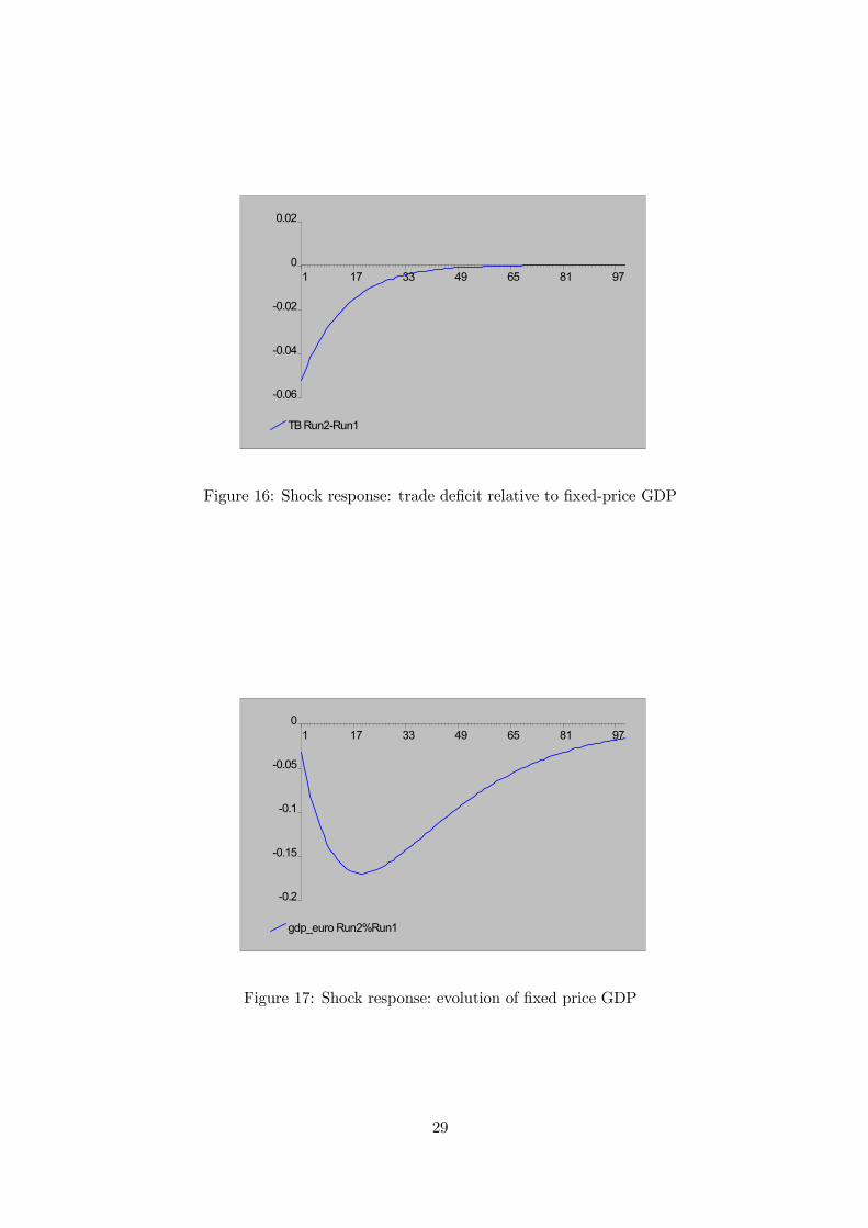
Figure 16: Shock response: trade deficit relative to fixed-price GDP

gdp_euro Run2%Run1

-0.2

-0.15

-0.1

-0.05

0 1 17 33 49 65 81 97

Figure 17: Shock response: evolution of fixed price GDP

29

5.2.2 Faster capital adjustment

This case corresponds to c = 5000 (instead of 3000). An initial shock in capital has a half-time

of 1.5 years (15 periods), somewhat still slower than the speed of the nominal adjustment.

The fall in capital is larger, but its level also returns faster to normal. All other impulse

responses are very similar to the baseline. The cumulative loss of GDP is 1076 basis points,

somewhat larger than the baseline number.

5.2.3 Initial capital stock

Instead of 100%, I also explored the choice of 90%. The loss of capital is somewhat larger, just

like the initial increase of the nontraded-traded relative price. The cumulative loss of GDP, on

the other hand, is only 854 basis points (in absolute terms, there is a smaller loss of capital). In

fact, there is even an increase at the beginning.

5.2.4 Different speeds of nominal adjustment

Instead of V = 0.1, I have explored a faster (V = 0.2, a half life of an H-shock is 5 periods) and

a slower (V = 0.05, a half life of 18 periods) adjustment scenario. The results (not reported) are

easy to interpret: the impact effect on the relative price is largely independent from V . Under

fast nominal adjustment, the price level quickly returns to equilibrium, so there is little response

by capital accumulation. Cumulative GDP loss is also smaller, with the particular choice of

V , the reduction is substantial (287 basis points of per period GDP). Under slow adjustment,

all statements are reversed, capital accumulation is seriously affected, which translates into a

cumulative GDP loss of 2745 basis points of per period GDP.

5.2.5 Initial money stock

I have checked the implications of varying H0 by ±10%. In other words, it means that I

check the implications of initial excess demand (+10%, overvaluation) and excess supply (−10%,undervaluation) on the responsiveness of the economy to nominal shocks. Under excess demand,

all the impulse responses are bigger, but not substantially. An overall indicator could be the

cumulative GDP loss number, which becomes 1063 basis points, somewhat larger than for the

baseline case. With undervaluation, all reactions are smaller, and the loss reduces to 802 basis

points.

5.3 Government spending

This has similar implications than a nominal appreciation, though the evolution of government

spending can have various dynamics, each producing different impulse responses. For example,

the government can distribute 10% of GNP to consumers immediately, or during a certain

number of periods. Later on, it might take it back or not (notice that such a future event is not

30

correctly handled by my approximately forward-looking consumers). Qualitatively, we get the

same answers as with a revaluation.

6 Discussion

The signs of the previous results are relatively easy to interpret. Both a fiscal expansion and

a revaluation increases the value of H in terms of traded goods. This leads to an increase

in spending on nontraded goods, which increases nontraded production. Given the short-run

nonlinearity of the transformation curve, nontraded prices must increase. This is the dominant

shock to the economy, all of the other results can be traced to this through the Stolper-Samuelson

theorem: if the price of a sector increases, it leads to a more than proportional increase in the

price of the factor which is used more intensively by the windfall sector. The price of the other

factor of production decreases.

In our case, the price of the nontraded sector has increased, and it is more labor-intensive.

This leads to a rise in wages and a fall in rental rates. Production becomes more capital-intensive,

and the fall in rental rates decreases capital inflows (q falls).

What makes this situation persistent? The explanation is closely related to the phenomenon

of ”Dutch disease”: a country receiving a transfer also sees its terms of trade improving. The

extra consumption enabled by the transfer falls partly on nontradables, which pushes domestic

wages up. In our two factor model, we need some extra conditions for the transfer effect: if the

only source of income of domestic consumers is their labor earnings, then the nontraded sector

must be more labor intensive than the traded sector. The price of capital falls, but that does

not influence domestic spending.

This is the underlying propagation mechanism: the initial shock to consumption increases

domestic income, so the excess money stock will flow out only slowly. If some of the capital is

domestic, and its income is used for consumption expenditures, then excess spending still creates

some of its excess income, but to a smaller degree. In this case, we can get persistence even

without the labor intensity assumption.

One can give a similar interpretation to the nominal convergence path starting from the

medium-term (real) equilibrium position: since the money accumulation process governed by

consumer optimization is not the same as the medium-term equilibrium path, period one money

stocks differ. This changes all prices in equilibrium, through the ”demand effect”. For a smaller

than equilibrium H, wages also become smaller, which then reinforces the initial undervaluation

and makes it persistent. Undervaluation thus even increases initially. This is balanced by the

effect on capital accumulation: due to a higher rental rate, there is more capital inflow, which

leads to an increase of wages eventually. Undervaluation starts to disappear. With my choice of

parameters (and approximations), the system converges to the equilibrium path (medium- and

long-term) through undervaluation. In general, it is possible to have a shift to overvaluation

during this process.

31

It is clear that the parameter V plays an important role in determining the speed of adjust-

ment through the trade balance: excess spending is proportional to VH, so a small V leads to

a slow outflow of the extra money. Looking one step behind, V is proportional to (δ + π) γ1−γ ,

the sum of the discount factor and inflation times the substitutability between consumption and

money holdings. Consequently, V represents the degree of intertemporal consumption smooth-

ing — how fast consumers deplete their excess money stocks. Another important determinant of

persistence is the weight of nontradables in consumption expenditures, since the larger it is, the

more valid the Keynesian thesis that ”excess demand creates its supply”.

It is important to note that the sectorial labor intensity (or the sectorial factor mobility)

assumption is not relevant for the increase of the price of nontradables. Its role is to make the

price of capital fall and wages increase (through the Stolper-Samuelson theorem). The ”wealth

effect” of a revaluation hurts or benefits capital (investment), depending on relative factor inten-

sities. I have explored a scenario with the traded sector being more labor intensive. Nontraded

prices increased, wages fell, the rental rate increased, and capital accumulation accelerated.

The degree of substitutability between the two goods (by consumers) and the factors of

production (by producers) also influences the quantitative behavior of the economy. Starting

with the preference side, let us assume that consumption utility is

µ(1− λ)

1θ C

θ−1θ

T + λ1θC

θ−1θ

NT

¶ θθ−1

.

The choice of θ = 1 corresponds to my Cobb-Douglas specification. Suppose that θ > 1.

An increase in p then implies a larger substitution towards traded goods, so an increase in

consumption expenditure must lead to a smaller increase in CNT and p. Keeping the same

transformation curve between traded and nontraded goods, a smaller price increase leads to

a smaller wage increase and a smaller decrease of the rental rate. This muted impact effect

also weakens the endogenous persistence of the shock, since a smaller wage increase leads to a

faster outflow of excess money. In summary, a higher degree of substitutability between traded

and nontraded goods increases both the impact effect and the persistence of nominal shocks

on the real economy. Conversely, θ < 1 increases both the impact effect and the persistence.

One can even find parameters such that a nominal appreciation initially improves the trade

balance (wages increase more than one in one relative to the nominal exchange rate). Later on,

the corresponding decline in r and K leads to a fall in w, and excess money flows out in the

long-run.

Intuitively, one would expect the opposite impact of substitutability between factors of pro-

duction: if it is easy to substitute labor with capital, then the same price increase leads to a

smaller wage increase. Consequently, the same increase in nontraded expenditure (pCNT ) leads

to a smaller increase in p and w, thus a smaller impact effect and smaller persistence. The com-

bination of nonunit substitutability both in preferences and technology has very complicated

32

general equilibrium cross-effects, which could be addressed only numerically.

Recent developments in the Hungarian economy (rising wages, stagnating investment, a

marked asymmetry between traded and nontraded investment behavior) suggest an overall de-

cline in rw . If we do not attribute this entirely to changes in minimum wages and public sector

wages, then the monetary restriction (”revaluation”) and the overall fiscal expansion offers an

explanation. Note that this requires the sectorial factor intensity assumption, which seems to

be somewhat problematic with Hungarian data. One resolution would be to assume similar fac-

tor intensities but then relax the equalization of rental rates across sectors. The reverse factor

intensity scenario should have counteracted the exogenous rise in wages, but there are no signs

for such an effect. Moreover, this would not have led to a rise in nontraded investment.

One comment is in line here, about the large sectorial reallocations showed by the results.

These are the consequences of the assumption that only the cross-border adjustment of capital

is slow. The price of domestic labor and installed domestic capital is equalized between the two

sectors, so there is free sectorial mobility. Regarding capital, this does not necessarily imply a

large reallocation: remember that all the results are in effective terms, so the capital stock is

constantly adjusted to TFP growth. A decline in effective capital stocks corresponds to a much

smaller decline or even an increase in regular capital. It seems plausible that current investment

is always channeled in a way that sectorial differences in rental rates are minimal. As long as

regular investment is positive in both sectors, the equalization of rental rates can be resolved

only through the appropriate allocation of new capital between sectors.

For labor, such an argument does not work, and one has good reasons to believe that labor

also adjusts slowly. This leads to sectorial wage differences, which is likely to increase the impact

effect of the nominal shocks (nontraded prices must increase even more, since near fixed capital

and labor imply a large increase in the cost of production), but its persistence should decrease

— by the time labor starts to switch sectors, the price and wage differentials have been nearly

eliminated. My results still issue a warning about the direction of asymmetries between sectors

and factors, and indicate the direction of reallocation. For example, with gradual labor flows,

nontraded prices should increase even more, nontraded sector wages should increase heavily,

while traded sector wages may even fall temporarily.

An important extension of the model is the following (this is also the direction of future

developments). Maintain the assumption of labor mobility, but allow for temporary firm profits,

and gradual capital flows between sectors and countries. One would then have monopolistic

competitors in the domestic nontraded and traded sectors, and also in the world traded market.

One can assume free entry (or even perfect competition) abroad, and a gradual entry and exit

of domestic firms in response to profits. In a q theory fashion, entry and exit could be a function

of current and expected future profits (discounted by world interest rates). This would allow

for a gradual passthrough of the nominal exchange rate into domestic tradable prices, and also

a more complete and realistic treatment of investment, profits and the reallocation of capital

between sectors.

33

One can reinterpret the ”money effect” as a ”wealth effect”, or even as a portfolio resizing

and rebalancing effect. The common feature is that a nominal shock will influence the value

or the returns of nominal wealth/assets, leading to a change in the intertemporal behavior of

consumers. Such a change will translate into a change in consumption expenditures, which is

the necessary starting point of my model.

In the wealth effect interpretation, it is implausible to assume that expenditures are deter-

mined entirely by wealth. In terms of a consumption function

E = µVH + (1− µ)Y,

I have assumed so far that µ is one (here H is total wealth, and not just money, though it does

not yet earn any returns). This implies that V controls both the steady state wealth-income

ratio and the persistence of the nominal shock response. The model can be extended to µ 6= 1,which yields

Kt = kT (t)

µ1 + λ (1− µ) β − α

1− β

¶+ λµV

H

ekT (t)

β

µ1− α

1− β− α

β

¶(16)

rt = (1− β) ekT (t)−β

Kt+1 =Kt+22 + r∗

+Kt (1 + r

∗)2 + r∗

+c

2 + r∗³rt³Kt´/e− r∗

´Ht+1 − Ht = e

1 + g(β + λ (1− µ) (2α− β)) kT

³Kt´1−β − V Ht

1 + g

1− β + λ (1− µ) (β − α) β−2αβ

1− β + λ (1− µ) (β − α).

The equations are somewhat more complicated, but they remained quite similar. It is visible

that both µ and V influence the persistence of shock responses. So far, I have not experimented

with solving (16).

7 Some concluding empirical considerations

There is vast literature on exchange rate based stabilizations (for example, Rebelo and Végh

(1995)), their stylized facts, the sources of success or failure. Darvas (2003) identifies two

main groups of countries who experienced large (nominal and real) appreciations at the start

of disinflations: fixed exchange rate, mostly Latin American countries with a failure in their

stabilization programs, and floating countries, mostly industrial, with a success. The question is

then whether these differences in country experiences can be related to differences in the strength

of the mechanisms of my model. Naturally, there are many additional issues and considerations

determining the overall success or failure (credibility, fiscal side, just to name a few), but this

”transfer effect” might also be an important contributor.

According to my results, a nominal appreciation has a negative side effect, through nontraded

prices: even if there is immediate and full passthrough of the nominal appreciation into tradable

34

prices, the ”equilibrium” (flexible price, but gradual adjustment of money balances/wealth) rel-

ative price of nontradables increases. Under certain factor intensity assumptions (the nontraded

sector is more labor intensive than the traded sector), it is also true that wages increase (relative

to tradable prices, which is the same as relative to wages in the rest of the world). Assume that

these qualitative effects are equally present in successful and failed disinflation episodes.

What can determine the difference in success? If nontraded inflation or wage inflation remains

relatively high, then expected inflation may adjust only little. If we manage to introduce inflation

persistence (expectations) into the model, then a slow adjustment of wages and nontraded prices

should increase inflation persistence (expectations), thus making the success of the disinflation

less probable. This interpretation would trace the difference in success or failure into differences

in the impact and persistence of the wealth (money) effect of an appreciation.

These differences can come from the role of money/wealth directly (like parameters V and

µ), or from different production functions, factor intensities, preferences, intertemporal and

intratemporal substitutability of goods. The distance from steady state (industrial country or

emerging market), or the role of capital income within GNP may also matter. Thinking in

terms of an external asset position, it may also matter whether the country is a net lender or

borrower, since a revaluation decreases the value of external assets, so it decreases the value of

outstanding foreign debt. Besides this direct wealth effect, there can be a portfolio rebalancing

between foreign and domestic assets as well.

These are all differences which can be measured for both groups of countries. For most

of them, one would expect that the failure countries are subject to larger wealth (nominal)

effects. It is central to have data on wages and nontraded-traded relative prices. Burstein et al

(2002) document a systematic behavior of prices after large devaluations: once one accounts for

various conceptual and measurement issues in tradable prices, the only remaining mystery is the

surprisingly low increase in nontradable prices. That effect can also be related to the negative

wealth or money effect of a devaluation, cutting domestic spending, thus decreasing the relative

price of nontradables.

Apart from data availability issues, a major problem of implementing this empirical cross-

country comparison is that success and failure countries also differed in their fiscal policies.

Overall, successful countries did not tend to ”match” the appreciation with a fiscal expansion,

which is much less true for failure countries. As argued earlier, a fiscal expansion has qualitatively

similar implications for relative prices and factor rewards as an appreciation. In order to relate

success or failure to a different money or wealth effect, one needs to filter out the effect of fiscal

policy. It is in fact possible that fiscal policy gets all the blame of a failure, but it may also

happen that disinflation would have failed even without a fiscal expansion. Unfortunately, this

filtering might require extensive data on government behavior, and its result might be sensitive

to parameters and model specification.

The last piece of speculation concerns the reason for certain countries switching to a fiscal

expansion around the appreciation. Is there a potential mechanism that leads to an automatic

35

fiscal expansion, depending on the equilibrium implications and price incidence of the nominal

appreciation? For example, a government closely allied with exporters or domestic capital owners

might be tempted to compensate domestic firms for the strong exchange rate. A government

concerned with slowing investment may also adopt a fiscal expansion. The common theme is

that an appreciation hurts exporters and capital, and a fiscal policy aimed at offsetting these

effects ends up giving substantial extra income to domestic consumers as a byproduct.

References

[1] Benabou, R. és K. Fukao: History versus Expectations: A Comment, Quarterly Journal of

Economics, 1993.

[2] Benczúr, P. and I. Kónya: Continuous Time Real Appreciation Model, mimeo, 2003.

[3] Benczúr, P., A. Simon and V. Várpalotai: Evaluating Macroeconomic Strategies with a

Calibrated Model, mimeo, 2003.

[4] Burstein, A., Eichenbaum, M., and S. Rebelo: Why is Inflation so Low after Large Deval-

uations?, NBER Working Paper 8748, 2002.

[5] Darvas, Zs.: Analysis of large real exchange rate appreciations; MNB Background Studies,

2003/2.

[6] Dornbusch. R.: Open Economy Macroeconomics, Chapter 6, Basic Books.

[7] Dornbusch, R. and M. Mussa: Consumption, Real Balances and the Hoarding Function,

International Economic Review, 1975.

[8] Krugman, P.: History versus Expectations, Quarterly Journal of Economics, 1991.

[9] Obstfeld, M. and K. Rogoff: Foundations of International Macroeconomics, Chapter 4, The

MIT Press, 1996.

[10] Pula, G.: ,Capital Stock Estimation in Hungary: A Brief Description of Methodolgy and

Results, MNB Working Paper, 2003/7.

[11] Rebelo, S. and C. A. Végh: Real Effects of Exchange-Rate Based Stabilization: An Analysis

of Competing Theories, in NBER Macroeconomics Annual, 1995.

[12] Simon, A. and V. Várpalotai: Oprimal Indebtendness of a Small Open Economy with

Precautionary Behavior, MNB Working Paper 2001/1.

[13] Stein, J.: The Natural Real Exchange Rate of the United States Dollar and Determinants

of Capital Flows, in J. Williamson (ed.), Estimating Equilibrium Exchange Rates, Institute

for International Economics, Washington D.C., 1994.

36

Appendix

From profit maximization in T:

r = (1− β) ek−βTw = βek1−βT .

Using the labor optimality condition in NT:

αpNT k1−αNT = βek1−βT ,

so

pNT =βek1−βT

αk1−αNT

.

Plugging into the capital optimality conditions:

(1− β) ek−βT = r = (1− α) pNT k−αNT = (1− α)βek1−βT

k−αNTαk1−αNT

=1− α

αβek1−βT k−1NT ,

so

kNT =1− α

α

β

1− βkT

and

pNT =βek1−βT

αk1−αNT

= eβ

α

µ1− α

α

β

1− β

¶α−1kα−βT .

Let us write down the demand for nontraded goods:

λVH = pNTCNT . (17)

In the nontraded sector, demand must equal supply (one cannot import or export nontradables

by definition), so

CNT = YNT = LαNTK

1−αNT = KNTk

−αNT .

37

Substituting this into (17):

KNT = CNTkαNT =

λVH

pNTkαNT =

λVH¡pNT/Aα

T

¢ (kNT/AT )αKNTAT

= λV HkαNTpNT

=λV H

e

³1−αα

β1−β kT

´αβα

³1−αα

β1−β

´α−1kα−βT

=λV H

e

1− α

1− βkβT .

We already have the effective capital-labor ratio in the nontraded sector, and the effective capital

stock as well, so we can obtain an expression for labor:

LNT =KNTkNT

=KNT/ATkNT/AT

=

λV He

1−α1−β k

βT

1−αα

β1−β kT

=λV H

e

α

βkβ−1T ,

so labor market clearing implies

LT = 1− LNT = 1− λVH

e

α

βkβ−1T ,

and

KT = LTkT = LTAT kT .

Finally, the capital market clearing condition is

K = KT +KNT = LTAT kT + λVH

e

1− α

1− βkβTAT = AT kT − λV

H

e

α

βkβTAT + λV

H

e

1− α

1− βkβTAT

= AT kT + λV ATH

ekβT

µ1− α

1− β− α

β

¶.

38

MNB Füzetek / MNB Working Papers

1995/1 SIMON András: Aggregált kereslet és kínálat, termelés és külkereskedelem a magyar gazdaságban1990-1994Aggregate Demand and Supply, Production and Foreign Trade in the Hungarian Economy, 1990-1994(available only in Hungarian)

1995/2 NEMÉNYI Judit: A Magyar Nemzeti Bank devizaadósságán felhalmozódó árfolyamveszteség kérdéseiIssues of Foreign Exchange Losses of the National Bank of Hungary (available only in Hungarian)

1995/3 DR. KUN János: Seignorage és az államadóság terheiSeigniorage and the Burdens of Government Debt (available only in Hungarian)

1996/1 SIMON András: Az infláció tényezői 1990-1995-benFactors of Inflation, 1990-1995 (available only in Hungarian)

1996/2 NEMÉNYI Judit: A tőkebeáramlás, a makrogazdasági egyensúly és az eladósodási folyamatösszefüggései a Magyar Nemzeti Bank eredményének alakulásávalThe Influence of Capital Flows, Macroeconomic Balance and Indebtedness on the Profits of theNational Bank of Hungary (available only in Hungarian)

1996/3 SIMON András: Sterilizáció, kamatpolitika az államháztartás és a fizetési mérlegSterilization, Interest Rate Policy, the Central Budget and the Balance of Payments (available only in Hungarian)

1996/4DARVAS Zsolt: Kamatkülönbség és árfolyam-várakozásokInterest Rate Differentials and Exchange Rate Expectations (available only in Hungarian)

1996/5 VINCZE János – ZSOLDOS István: A fogyasztói árak struktúrája, szintje és alakulása Magyarországon1991-1996-ban; Ökonometriai vizsgálat a részletes fogyasztói árindex alapjánThe Structure, Level and Development of Consumer Prices in Hungary, 1991-1996 – An EconometricAnalysis Based on the Detailed Consumer Price Index (available only in Hungarian)

1996/6 CSERMELY Ágnes: A vállalkozások banki finanszírozása Magyarországon 1991-1994Bank Financing of Enterprises in Hungary, 1991-1994 (available only in Hungarian)

1996/7 DR. BALASSA Ákos: A vállalkozói szektor hosszú távú finanszírozásának helyzete és fejlődési irányaiThe Development of Long-term Financing of the Enterprise Sector (available only in Hungarian)

1997/1CSERMELY Ágnes: Az inflációs célkitűzés rendszereThe Inflation Targeting Framework (available only in Hungarian)

1997/2 VINCZE János: A stabilizáció hatása az árakra, és az árak és a termelés (értékesítés) közöttiösszefüggésekreThe Effects of Stabilization on Prices and on Relations Between Prices and Production (Sales) (available only in Hungarian)

1997/3 BARABÁS Gyula – HAMECZ István: Tőkebeáramlás, sterilizáció és pénzmennyiségCapital Inflow, Sterilization and the Quantity of Money

1997/4 ZSOLDOS István: A lakosság megtakarítási és portfolió döntései Magyarországon 1980-1996Savings and Portfolio Decisions of Hungarian Households, 1980-1996 (available only in Hungarian)

1997/5 ÁRVAI Zsófia: A sterilizáció és tőkebeáramlás ökonometriai elemzéseAn Econometric Analysis of Capital Inflows and Sterilization (available only in Hungarian)

1997/6 ZSOLDOS István: A lakosság Divisia-pénz tartási viselkedése MagyarországonCharacteristics of Household Divisia Money in Hungary (available only in Hungarian)

1998/1 ÁRVAI Zsófia – VINCZE János: Valuták sebezhetősége: Pénzügyi válságok a ‘90-es évekbenVulnerability of Foreign Currency: Financial Crises in the 1990s (available only in Hungarian)

1998/2 CSAJBÓK Attila: Zéró-kupon hozamgörbe becslés jegybanki szemszögbőlZero-coupon Yield Curve Estimation from a Central Bank Perspective

1998/3 KOVÁCS Mihály András - SIMON András: A reálárfolyam összetevőiComponents of the Real Exchange Rate in Hungary

1998/4 P.KISS Gábor: Az államháztartás szerepe MagyarországonThe Role of General Government in Hungary

1998/5 BARABÁS Gyula – HAMECZ István – NEMÉNYI Judit: A költségvetés finanszírozási rendszerénekátalakítása és az eladósodás megfékezése; Magyarország tapasztalatai a piacgazdaság átmenetiidőszakábanFiscal Consolidation, Public Debt Containment and Disinflation; Hungary’s Experience in Transition

1998/6 JAKAB M. Zoltán – SZAPÁRY György: A csúszó leértékelés tapasztalatai MagyarországonHungary’s Experience of the Crawling Peg System (available only in Hungarian)

1998/7 TÓTH István János – VINCZE János: Magyar vállalatok árképzési gyakorlataPricing Behaviour of Hungarian Firms (available only in Hungarian)

1998/8 KOVÁCS Mihály András: Mit mutatnak? Különféle reálárfolyam-mutatók áttekintése és a magyargazdaság ár- és költség-versenyképességének értékeléseThe Information Content of Real Exchange Rate Indicators (available only in Hungarian)

1998/9 DARVAS Zsolt: Moderált inflációk csökkentése; Összehasonlító vizsgálat a nyolcvanas-kilencvenes évekdezinflációit kísérő folyamatokrólModerate Inflations: a Comparative Study (available only in Hungarian)

1998/10 ÁRVAI Zsófia: A piaci és kereskedelmi banki kamatok közötti transzmisszió 1992 és 1998 közöttThe Interest Rate Transmission Mechanism between Market and Commercial Bank Rates

1998/11 P. KISS Gábor: A költségvetés tervezése és a fiskális átláthatóság aktuális problémáiTopical Issues of Fiscal Transparency and Budgeting (available only in Hungarian)

1998/12 JAKAB M. Zoltán: A valutakosár megválasztásának szempontjai MagyarországonDeriving an Optimal Currency Basket for Hungary (available only in Hungarian)

1999/1 CSERMELY Ágnes – VINCZE János: Leverage and foreign ownership in Hungary Tőkeáttétel és külföldi tulajdon (csak angol nyelven)

1999/2 TÓTH Áron: Kísérlet a hatékonyság empirikus elemzésére a magyar bankrendszerbenAn Empirical Analysis of Efficiency in the Hungarian Banking System (available only in Hungarian)

1999/3DARVAS Zsolt – SIMON András: A növekedés makrogazdasági feltételei; Gazdaságpolitikai alternatívákCapital Stock and Economic Development in Hungary

1999/4 LIELI Róbert: Idősormodelleken alapuló inflációs előrejelzések; Egyváltozós módszerekInflation Forecasting Based on Series Models. Single-Variable Methods (available only in Hungarian)

1999/5 FERENCZI Barnabás: A hazai munkaerőpiaci folyamatok Jegybanki szemszögből – Stilizált tényekLabour Market Developments in Hungary from a Central Bank Perspective – Stylized Facts

1999/6 JAKAB M. Zoltán – KOVÁCS Mihály András: A reálárfolyam-ingadozások főbb meghatározóiMagyarországonDeterminants of Real-Exchange Rate Fluctuations in Hungary

1999/7 CSAJBÓK Attila: Information in T-bill Auction Bid Distributions Az aukciós kincstárjegyhozamok információs tartalma (csak angol nyelven)

1999/8 BENCZÚR Péter: A magyar nyugdíjrendszerben rejlő implicit államadósság-állomány változásánakbecsléseChanges in the Implicit Debt Burden of the Hungarian Social Security System

1999/9 VÍGH-MIKLE Szabolcs – ZSÁMBOKI Balázs: A bankrendszer mérlegének denominációs összetétele 1991-1998 közöttDenomination Structure of the Balance Sheet of the Hungarian Banking Sector, 1991-1998 (availableonly in Hungarian)

1999/10 DARVAS Zsolt – SZAPÁRY György: A nemzetközi pénzügyi válságok tovaterjedése különbözőárfolyamrendszerekben Financial Contagion under Different Exchange Rate Regimes

1999/11 OSZLAY András: Elméletek és tények a külföldi működőtőke-befektetésekrőlTheories and Facts about Foreign Direct Investment in Hungary (available only in Hungarian)

2000/1JAKAB M. Zoltán – KOVÁCS Mihály András – OSZLAY András: Hová tart a külkereskedelmi integráció?Becslések három kelet-közép-európai ország egyensúlyi külkereskedelméreHow Far has Trade Integration Advanced? An Analysis of Actual and Potential Trade by Three Centraland Eastern European Countries

2000/2 VALKOVSZKY Sándor –VINCZE János: Estimates of and Problems with Core Inflation in Hungary A maginfláció becslése és problémái (csak angol nyelven)

2000/3 VALKOVSZKY Sándor: A magyar lakáspiac helyzete Situation of the Hungarian Housing Market (available only in Hungarian)

2000/4 JAKAB M. Zoltán – KOVÁCS Mihály András – LŐRINCZ Szabolcs: Az export előrejelzése ökonometriaimódszerekkelForecasting Hungarian Export Volume

2000/5 FERENCZI Barnabás – VALKOVSZKY Sándor – VINCZE János: Mire jó a fogyasztói-ár statisztika? What are Consumer Price Statistics Good for?

2000/6 ÁRVAI Zsófia – VINCZE János: Financial Crises in Transition Countries: Models and FactsPénzügyi válságok átmeneti gazdaságokban: modellek és tények (csak angol nyelven)

2000/7 György SZAPÁRY: Maastricht and the Choice of Exchange Rate Regime in Transition Countries duringthe Run-Up to EMUMaastricht és az árfolyamrendszer megválasztása az átmeneti gazdaságokban az EMU csatlakozástmegelőzően (csak angol nyelven)

2000/8 ÁRVAI Zsófia – MENCZEL Péter: A magyar háztartások megtakarításai 1995 és 2000 közöttSavings of Hungarian Households, 1995-2000

2000/9 SIMON András – DARVAS Zsolt: A potenciális kibocsátás becslése a gazdaság nyitottságánakfelhasználásávalPotential Output and Foreign Trade in Small Open Economies

2001/1 SIMON András – VÁRPALOTAI Viktor: Eladósodás, kockázat és óvatosságOptimal Indebtedness of a Small Open Economy with Precautionary Behavior

2001/2 TÓTH István János - ÁRVAI Zsófia: Likviditási korlát és fogyasztói türelmetlenségLiquidity constraints and consumer impatience

2001/3Sándor VALKOVSZKY – János VINCZE: On Price Level Stability, Real Interest Rates and Core InflationÁrszintstabilitás, reálkamat és maginfláció (csak angol nyeleven)

2001/4János VINCZE: Financial Stability, Monetary Policy and Integration: Policy Choices for TransitionEconomies Pénzügyi stabilitás, monetáris politika, integráció: az átmeneti gazdaságok előtt álló választásilehetőségek (csak angol nyelven)

2001/5György SZAPÁRY: Banking Sector Reform in Hungary: Lessons Learned, Current Trends and ProspectsA bankrendszer reformja Magyarországon: tanulságok, aktuális folyamatok és kilátások (csak angol nyelven)

2002/1TÓTH István János: Vállalati és lakossági konjunktúra felmérések MagyarországonCyclical Surveys of the Hungarian Corporate and Household Sectors (available only in Hungarian)

2002/2BENCZÚR Péter: A szuverén kötvényekben rejlő kockázatok azonosítása Identifying Sovereign Bond Risks (available only in Hungarian)

2002/3JAKAB M. Zoltán – KOVÁCS Mihály András: Magyarország a NIGEM modellbenHungary in the NIGEM model

2002/4BENCZÚR Péter – SIMON András – VÁRPALOTAI Viktor: Dezinflációs számítások kisméretű makromodellelDisinflation Simulations with a Small Model of an Open Economy (available only in Hungarian)

2002/5On the estimated size of the Balassa-Samuelson effect in five Central and Eastern European countries Edited by Mihály András KOVÁCS (avaible only in English)

2002/6GYOMAI György - VARSÁNYI Zoltán Máté: Az MNB átlal használt hozamgörbe-becslő eljárásfelülvizsgálata A Comparison of Yield-curve Fitting Methods for Monetary Policy Purposes in Hungary (available only inHungarian)

2003/1Péter BENCZÚR: The behavior of the nominal exchange rate at the beginning of disinflations (availableonly in English)

2003/2VÁRPALOTAI Viktor: Numerikus módszer gazdasági adatok visszabecsléséreNumerical Method for Estimating GDP Data for Hungary (available only in Hungarian)

2003/3VÁRPALOTAI Viktor: Dezinflációs számítások dezaggregált kibocsátási résekre alapzó makromodellelDisinflation Simulations with a Disaggregated Output Gap Based Model (available only in Hungarian)

2003/4VÁRPALOTAI Viktor: Dezaggregált költségbegyűrűzés-alapú ökonometriai infláció-előrejelző modellDisaggregated Cost Pass-Through Based Econometric Inflation-Forecasting Model for Hungary

2003/5Zoltán M. JAKAB-Mihály András KOVÁCS: Explaining the Exchange Rate Pass-Through in Hungary:Simulations with the NIGEM Model (available only in English)

2003/6Gábor VADAS: Modelling households’ savings and dwellings investment – a portfolio choice approach(available only in English)

2003/7Gábor PULA: Capital Stock estimation in Hungary: A brief description of methodology and results(avaiable ony in English)

2003/8Zsolt DARVAS-GÁBOR VADAS: Univariate Potential Output Estimations for Hungary (avaiable only in English)

2003/9Péter BENCZÚR: Nominális sokkok átmeneti reálhatása egy kétszektoros növekedési modellbenReal Effects of Nominal shocks: a 2-sector Dynamic Model with Slow Capital Adjustment and Money-in-the-utility