arX

iv:1

304.

5343

v1 [

astr

o-ph

.SR

] 19

Apr

201

3Astronomy & Astrophysicsmanuscript no. arxisubmit˙2column c© ESO 2013April 22, 2013

High rigidity Forbush decreases: due to CMEs or shocks?Arun Babu1, H. M. Antia2, S. R. Dugad2, S. K. Gupta2, Y. Hayashi3, S. Kawakami3, P. K. Mohanty2, T. Nonaka3, A.

Oshima4, P. Subramanian1(The GRAPES-3 Collaboration)

1 Indian Institute of Science Education and Research, Sai Trinity Building, Pashan, Pune 411 021, India2 Tata Institute of Fundamental Research, Homi Bhabha Road, Mumbai 400 005, India

The GRAPES–3 Experiment, Cosmic Ray Laboratory, Raj Bhavan, Ooty 643 001, India3 Graduate School of Science, Osaka City University, Osaka 558-8585, Japan4 National Astronomical Observatory of Japan, CfCA, Tokyo 181-8588, Japan

ABSTRACT

Aims. We seek to identify the primary agents causing Forbush decreases (FDs) observed at the Earth in high rigidity cosmic rays. Inparticular, we ask if such FDs are caused mainly by coronal mass ejections (CMEs) from the Sun that are directed towards the Earth,or by their associated shocks.Methods. We use the muon data at cutoff rigidities ranging from 14 to 24 GV from the GRAPES-3 tracking muon telescope toidentify FD events. We select those FD events that have a reasonably clean profile, and can be reasonably well associated with anEarth-directed CME and its associated shock. We employ two models: one that considers the CME as the sole cause of the FD (theCME-only model) and one that considers the shock as the only agent causing the FD (the shock-only model). We use an extensiveset of observationally determined parameters for both these models. The only free parameter in these models is the levelof MHDturbulence in the sheath region, which mediates cosmic ray diffusion (into the CME, for the CME-only model and across the shocksheath, for the shock-only model).Results. We find that good fits to the GRAPES-3 multi-rigidity data using the CME-only model require turbulence levels in the CMEsheath region that are only slightly higher than those estimated for the quiet solar wind. On the other hand, reasonable model fits withthe shock-only model require turbulence levels in the sheath region that are an order of magnitude higher than those in the quiet solarwind.Conclusions. This observation naturally leads to the conclusion that theEarth-directed CMEs are the primary contributors to FDsobserved in high rigidity cosmic rays.

Key words. Forbush decrease, Coronal mass ejection(CME), Cosmic rays

1. Introduction

Forbush decreases are short-term decreases in the intensity ofthe galactic cosmic rays at the Earth. They are typically causedby the effects of interplanetary counterparts of coronal massejections (CMEs) from the Sun, and also the corotating inter-action regions (CIRs) between the fast and slow solar windstreams from the Sun. We concentrate on CME driven Forbushdecreases in this paper. The near-Earth manifestations of CMEsfrom the Sun typically have two major components: the inter-planetary counterpart of the CME, commonly called an ICME,and the shock which is driven ahead of it. ICMEs which pos-sess certain well-defined criteria such as plasma temperaturedepressions and smooth magnetic field rotations (e.g., Burlagaet al. 1981, Bothmer & Schwenn 1998) are called magneticclouds, while others are often classified as “ejecta”. The rela-tive contributions of shocks and ICMEs in causing Forbush de-creases is a matter of debate. For instance, Zhang & Burlaga(1988), Lockwood, Webber, & Debrunner (1991) and Reames,Kahler & Tylka (2009) argue against the contribution of mag-netic clouds to Forbush decreases. On the other hand, otherstudies (e.g., Badruddin, Yadav, & Yadav, 1986; Sanderson etal.,1990; Kuwabara et al 2009) concluded that magnetic cloudscan make an important contribution to FDs. There have beenrecent conclusive associations of Forbush decreases with Earth-directed CMEs (Blanco et al 2013; Oh & Yi 2012). Cane (2000)

introduced the concept of a “2-step” FD, where the first stepof the decrease is due to the shock and the second one is dueto the ICME. Based on an extensive study of ICME-associatedForbush decreases at cosmic ray energies between 0.5 – 450MeV, Richardson and Cane (2011) conclude that shock andICME effects are equally responsible for the Forbush decrease.They also find that ICMEs that can be classified as magneticclouds are usually involved in the largest of the Forbush de-creases they studied. From now on, we will use the term “CME”to denote the CME near the Sun, as well as its counterpart ob-served at the Earth.

In this paper we have used Forbush decrease data fromGRAPES-3 tracking muon telescope located at Ooty (11.4◦Nlatitude, 76.7◦E longitude, and 2200 m altitude) in south India.The GRAPES-3 muon telescope records the flux of muons innine independent directions (labeled NW, N, NE, W, V, E, SW,S and SE), and the geomagnetic cutoff rigidity over this fieldof view varies from 12 to 42 GV. The details of this telescopeare discussed in Hayashi et al. (2005), Nonaka et al. (2006) andSubramanian et al (2009). Thus, the GRAPES-3 telescope ob-serves the cosmic ray muon flux in nine independent directionswith varying cut-off rigidities simultaneously. The high muoncounting rate measured by the GRAPES-3 telescope results inextremely small statistical errors, allowing small changes in theintensity of the cosmic ray flux to be measured with high preci-

1

Arun Babu et al.: High rigidity Forbush decreases

Fig. 1. A schematic of the CME-shock system. The CME ismodeled as a flux rope structure. The undulating lines ahead ofthe shock denote MHD turbulence driven by the shock, whilethose in the CME sheath region denote turbulence in that region.

sion. Thus a small drop (∼0.2%) in the cosmic ray flux duringa Forbush decrease event can be reliably detected. This is possi-ble even in the presence of the diurnal anisotropy of much largermagnitude (∼1.0%), through a filtering technique described inSubramanian et al (2009) (referred to hereafter as S09).

A schematic of the CME, which is assumed to have a flux-rope geometry (Vourlidas et al 2012) together with the shockitdrives, is shown in Figure 1. The shock drives turbulence aheadof it, and there is also turbulence in the CME sheath region (e.g.,Manoharan et al 2000; Richardson & Cane 2011).

Instead of treating the entire system shown in Figure 1,which would be rather involved, we consider two separate mod-els. The first, that we call the “CME-only” model, is one wherethe Forbush decrease is assumed to be exclusively due to theCME, which is progressively populated by high energy cosmicrays as it propagates from the Sun to the Earth. The preliminaryidea behind this model was first sketched by Cane, Richardson& Wibberenz (1995) and developed in detail in S09. The workdescribed here addresses multi-rigidity data, which is a majorimprovement over S09. We will describe several other salientimprovements in the CME-only model in subsequent sections.The second model, which we call the “shock-only” model, isone where the Forbush decrease is assumed arise only due to apropagating diffusive barrier, which is the shock driven by theCME (e.g., Wibberenz et al 1998). The diffusive barrier wouldact as a shield for the galactic cosmic ray flux, resulting in alower cosmic ray density behind it. In treating these two modelsseparately, we aim to identify which is the dominant contributorto the observed Forbush decrease; the CME, or the shock.

We identify Forbush decreases in the GRAPES-3 data thatare associated with both near-Earth magnetic clouds and possi-bly shocks driven by them. We describe our event shortlistingcriteria in the next section. We then test the extent to whicheachof the models (the CME-only and the shock-only model) satis-fies the multi-rigidity Forbush decrease data from the GRAPES-3 muon telescope. In the subsequent analysis the use of cutoff

rather than median rigidity is preferred for the following reason.The cutoff rigidity in a given direction represents the thresholdrigidity of incoming cosmic rays and the magnitude of Forbushdecrease is a sensitive function of it. On the other hand the me-dian rigidity is comparatively insensitive to the magnitude of theForbush decrease.

2. Event shortlisting criteria

2.1. First and second shortlists: characteristics of theForbush decrease

We have examined all Forbush decrease events observed by theGRAPES-3 muon telescope from 2001 to 2004. We then short-listed events that have magnitudes> 0.25 % and possess a ‘rela-tively clean’ profile comprising a sudden decrease followedby agradual exponential recovery. While the figure of 0.25 % mightseem rather small by neutron monitor standards, we emphasizethat the largest events observed with GRAPES-3 have magni-tudes of∼ 1 %. This list, which contains 72 events, is calledshortlist 1. We next correlate the events in shortlist 1 withlistsof magnetic clouds near the Earth observed by the WIND andACE spacecrafts (Huttunen et al 2005; Lynch et al. 2003; A.Lara, private communication) and select only those that canbereasonably well connected with a near-Earth magnetic cloudandthis set is labeled shortlist 2 (Table 1). The decrease minimumfor most of the FD events in shortlist 2 lie between the start andthe end of the near-Earth magnetic cloud.

2.2. Third shortlist: CME velocity profile

Since we are looking for Forbush decrease events that are associ-ated with shocks as well as CMEs, we examine the CME catalog(http : //cdaw.gs f c.nasa.gov/CME list/) for a near-Sun CMEthat can reasonably correspond to the near-Earth magnetic cloudthat we associated with the Forbush decrease in forming shortlist2. In S09 it was assumed that the CME propagates with a con-stant speed from the Sun to the Earth. In this paper, we adopt amore realistic, two-step velocity profile that is describedbelow.

The data from the LASCO coronograph aboard the SOHOspacecraft (http : //cdaw.gs f c.nasa.gov/CME list/) providedetails about CME propagation up to a distance of≈ 30 R⊙ fromthe Sun. We fit the following velocity profile to the LASCO datapoints:

V1 = vi + ai t , for R(t) ≤ Rm (1)

where vi and ai are the initial velocity and acceleration of CMErespectively, andRm is the heliocentric distance at which theCME is last observed in the LASCO field of view. For distances> Rm, we assume that the CME dynamics are governed exclu-sively by the aerodynamic drag it experiences due to momentumcoupling with the ambient solar wind. For heliocentric distances> Rm, we therefore use the following widely used 1D differentialequation to determine the CME velocity profile: (e.g., Borgazziet al 2009)

mCMEV2∂V2

∂R=

12

CDρswACME(V2 − Vsw)2 , R(t) > Rm (2)

where mCME is the CME mass, CD is the dimensionless dragcoefficient,ρsw is the solar wind density, ACME = πR2

CME is thecross-sectional area of the CME and Vsw is the solar wind speed.The boundary condition used is V2 = vm at R(t)= Rm. The CMEmass mCME is assumed to be 1015 g and the solar wind speedVsw is taken to be equal to 450 km/s. The solar wind densityρswis given by the model of Leblanc et al (1998). The compositevelocity profile for the CME is defined by

VCME =

{

V1 , R(t) ≤ Rm

V2 , R(t) > Rm

(3)

The total travel time for the CME is∫ Rf

RidR/VCME, where Ri is

the heliocentric radius at which the CME is first detected andRf

2

Arun Babu et al.: High rigidity Forbush decreases

Table 1.Selected Events

Event Magnitude(Ver) (%) FD onset (UT) FD min (UT) MC start (UT) MC stop (UT) CME launch (UT)11/04/01 2.86 11/04/01, 12:00 12/04/01, 18:00 11/04/01, 23:00 12/04/01, 18:00 10/04/01, 05:3017/08/01 1.03 16/08/01, 22:34 18/08/01, 05:00 18/08/01, 00:00 18/08/01, 21:30 15/08/0 1, 23:5429/09/01 2.44 29/09/01, 12:43 31/09/01, 01:00 29/09/01, 16:30 30/09/01, 11:30 . . . not clear. . .24/11/01 1.56 24/11/01, 03:21 25/11/01, 15:00 24/11/01, 17:00 25/11/01, 13:30 22/11/01, 22:4823/05/02 0.93 23/05/02, 02:10 23/05/02, 23:00 23/05/02, 21:30 25/05/02, 18:00 . . . not clear. . .7/09/02 0.97 7/09/02, 14:52 8/09/02, 13:00 7/09/02, 17:00 8/09/02, 16:30 05/09/01, 16:5430/09/02 0.97 30/09/02, 11:30 31/09/02, 08:00 30/09/02, 22:00 1/09/02, 16:30 . . . not clear. . .20/11/03 1.16 20/11/03, 10:48 24/11/03, 04:00 21/11/03, 06:10 22/11/03, 06:50 18/11/03, 08:5026/07/04 2.13 26/07/04, 15:36 27/07/04, 11:00 27/07/04, 02:00 28/07/04, 00:00 25/07/04, 14:54

Notes.Events that can clearly be associated with near-Sun CMEs andagree with the composite velocity profile (§ 2.2) have a CME launch time(near the Sun) mentioned against them. These events form ourfinal shortlist (shortlist 3).Magnitude(Ver) : Magnitude of Forbush decrease in verticaldirectionFD onset : Time of FD onset in UTFD minimum : Time of FD minimum in UTMC start : Magnetic cloud start time in UTMCstop : Magnetic cloud stop time in UTCME near Sun : Time at which CME was first observed in the LASCO FOV

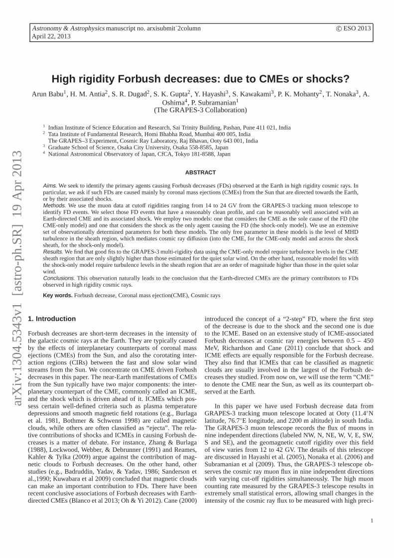
Fig. 2. A plot of the velocity profile for the CME correspond-ing to the 24 November 2001 FD event. The CME was first ob-served in the LASCO FOV on 22 November 2001. The solid lineshows the first stage governed by LASCO observations (Eq 1),where the CME is assumed to have a constant deceleration. Thedashed line shows the second stage (Eq 2), where the the CMEis assumed to experience an aerodynamic drag characterizedbya constant CD.

is equal to 1 AU. We have used a constant drag coefficient CDand adjusted its value so that the total travel time thus calculatedmatches the time elapsed between the first detection of the CMEin the LASCO FOV and its detection as a magnetic cloud nearthe Earth. We have retained only those events for which it ispossible to find a constant CD and this criterion is satisfied. Wehave also eliminated magnetic clouds that could be associatedwith multiple CMEs. This defines our final shortlist, which wecall shortlist 3.The events that have an entry in the last columnlabeled ‘CME launch’ in Table 1 comprise shortlist 3. We notethat we have adjusted the parameter CD so that the final CMEspeed obtained from Eq (2) is close to the observed magneticcloud speed near the Earth. It is usually not possible to find aCD that will yield an exact match for the velocities as well asthe total travel times (e.g., Lara et al 2011). Figure 2 showsanexample of the composite velocity profile (given by Eqs 1 and 2)for one such representative CME: the one that was first observedin the LASCO FOV on 22 November 2001, and resulted in a FDon 24 November 2001.

3. Models for Forbush decreases

We apply two different models to the FD events in Table 1; thefirst one is the CME-only model, which assumes that the Forbushdecrease owes its origin only to the CME. The second one is theshock-only model, which assumes that the Forbush decrease isexclusively due to the shock, which is approximated as a diffu-sive barrier. Although both the shock and the CME are expectedto contribute to the Forbush decrease, our treatment seeks to de-termine which one of them is the dominant contributor at rigidi-ties ranging from 14 to 24 GV. Before describing the models, wediscuss the perpendicular diffusion coefficient.

3.1. Perpendicular diffusion coefficient

We use an isotropic perpendicular diffusion coefficient (D⊥) tocharacterize the penetration of cosmic rays across large scale, or-dered magnetic fields. We envisage a CME, which has a flux ropestructure, propagates outwards from the Sun, driving a shockahead of it (see, e.g., Vourlidas et al 2012). The flux rope CME-shock geometry is illustrated in Figure 1. The CME sheath re-gion between the CME and the shock is known to be turbu-lent (e.g., Manoharan et al 2000) and it is well accepted thatit has a significant role to play in determining Forbush decreases(Badruddin 2002; Yu et al 2010). The isotropic perpendiculardiffusion coefficient D⊥ characterizes the penetration of cosmicrays through the ordered, compressed large-scale magneticfieldnear the shock, as well as across the ordered magnetic field ofthe flux rope CME. In diffusing across the shock, the cosmic raysare affected by the turbulence ahead of the shock, and in diffus-ing across the magnetic fields bounding the flux rope CME, thecosmic rays are affected by the turbulence in the CME sheathregion.

The subject of charged particle diffusion across field lines inthe presence of turbulence is a subject of considerable research.Analytical treatments include the so-called “classical” scatteringtheory (e.g., Giacalone & Jokipii (1999) and references therein),and the nonlinear guiding center theory (Matthaeus et al 2003;Shalchi 2010) for perpendicular diffusion. Numerical treatmentsinclude Giacalone & Jokipii (1999), Casse et al (2002), Candia& Roulet (2004) and Tautz & Shalchi (2011). For our purposes,we seek a concrete, usable prescription for the D⊥ that can in-corporate as many observationally determined quantities as pos-

3

Arun Babu et al.: High rigidity Forbush decreases

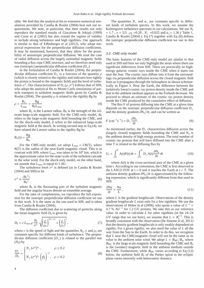
sible. We find that the analytical fits to extensive numericalsim-ulations provided by Candia & Roulet (2004) best suit our re-quirements. We note, in particular, that their results not onlyreproduce the standard results of Giacalone & Jokipii (1999)and Casse et al (2002) but also extend the regime of validityto include strong turbulence and high rigidities. Our approachis similar to that of Effenberger et al (2012), who adopt em-pirical expressions for the perpendicular diffusion coefficients.It may be mentioned, however, that they allow for the possi-bility of anisotropic perpendicular diffusion. We treat the caseof radial diffusion across the largely azimuthal magnetic fieldsbounding a flux rope CME structure, and we therefore need onlyone (isotropic) perpendicular diffusion coefficient (D⊥).

In the formulation of Candia & Roulet (2004), the perpen-dicular diffusion coefficient D⊥ is a function of the quantityρ(which is closely related to the rigidity and indicates how tightlythe proton is bound to the magnetic field) and the level of turbu-lenceσ2. Our characterization of D⊥(ρ, σ2) follows that of S09,who adopt the analytical fits to Monte Carlo simulations of par-ticle transport in turbulent magnetic fields given by Candia&Roulet (2004). The quantityρ is related to the rigidityRg by

ρ =RL

Lmax=

RgB0Lmax

(4)

whereRL is the Larmor radius, B0 is the strength of the rel-evant large-scale magnetic field. For the CME-only model,B0refers to the large-scale magnetic field bounding the CME, andfor the shock-only model, it refers to the enhanced large-scalemagnetic field at the shock. In writing second step in Eq (4), wehave related the Larmor radius to the rigidity Rg by

RL(t) =RgB0. (5)

For the CME-only model, we adopt Lmax = 2 R(T), whereR(T) is the radius of the near-Earth magnetic cloud. This is incontrast with S09, where Lmax was taken to be 106 km, which isthe approximate value for the outer scale of the turbulent cascadein the solar wind. For the shock-only model, on the other hand,we assume that Lmax is equal to 1 AU.

The turbulence levelσ2 is defined (as in Candia & Roulet[2004] and S09) to be

σ2 ≡〈Br

2〉

B02

(6)

where Br is the fluctuating part of the turbulent magneticfield and the angular braces denote an ensemble average.

For the sake of completeness, we reproduce the full expres-sion for the isotropic perpendicular diffusion coefficient we usein this work. It is the same as the one used in S09, and is takenfrom Candia & Roulet (2004).

The diffusion coefficient due to scattering of particles alongthe mean magnetic fieldD‖ is given by

D‖ = c LmaxρN‖σ2

√

(

ρ

ρ‖

)2(1−γ)

+

(

ρ

ρ‖

)2

, (7)

wherec is the speed of light and the quantitiesN‖, γ andρ‖ areconstants specific for different kinds of turbulence. The perpen-dicular diffusion coefficient (D⊥) is related to the parallel one(D‖) by

D⊥D‖=

N⊥ (σ2)a⊥ , ρ ≤ 0.2

N⊥ (σ2)a⊥

(

ρ

0.2

)−2

, ρ > 0.2(8)

The quantitiesN⊥ and a⊥ are constants specific to differ-ent kinds of turbulent spectra. In this work, we assume theKolmogorov turbulence spectrum in our calculations. We useN‖= 1.7 ,γ = 5/3 , ρ‖ =0.20 ,N⊥ =0.025 anda⊥= 1.36 ( Table 1,Candia & Roulet [2004] ). Eq (7) together with Eq (8) definesthe isotropic perpendicular diffusion coefficient we use in thiswork.

3.2. CME-only model

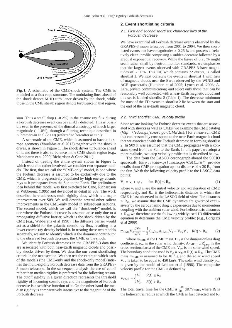
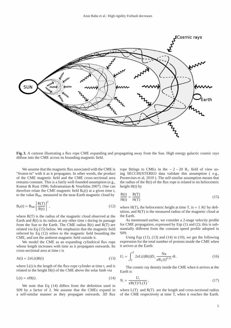
The basic features of the CME-only model are similar to thatused in S09 and here we only highlight the areas where there aresignificant differences from S09. There are practically no high-energy galactic cosmic rays inside the CME when it starts outnear the Sun. The cosmic rays diffuse into it from the surround-ings via perpendicular diffusion across the closed magnetic fieldlines as it propagates through the heliosphere as shown schemat-ically in Figure 3. Near the Earth, the difference between the(relatively lower) cosmic ray proton density inside the CMEandthat in the ambient medium appears as the Forbush decrease. Weproceed to obtain an estimate of the cosmic ray proton densityinside the CME produced by the cumulative effect of diffusion.

The flux F of protons diffusing into the CME at a given timedepends on the isotropic perpendicular diffusion coefficient D⊥and the density gradient∂Na/∂r, and can be written as

F (cm−2s−1) = D⊥∂Na

∂r. (9)

As mentioned earlier, the D⊥ characterizes diffusion across the(largely closed) magnetic fields bounding the CME and Na isthe ambient density of high energy protons. The total numberofcosmic ray protons that will have diffused into the CME after atime T is related to the diffusing flux by

Ui =

∫ T

0A(t)F(t) dt =

∫ T

0D⊥A(t)

∂Na

∂rdt (10)

where A(t) is the cross-sectional area of the CME at a giventime t. According to our convention, the CME is first observedinthe LASCO FOV at t= 0 and it reaches the Earth at t= T. Theambient density gradient∂Na/∂r is approximated by the follow-ing expression, which is significantly different from that used inS09:

∂Na∂r≃

NaL, (11)

whereL is the gradient lengthscale. Observations of the densitygradient lengthscaleL exist only for a few rigidities. We use theobservations of Heber et al (2008), who quote a value ofL−1 =

4.7 % AU−1 for 1.2 GV protons. We take this as our referencevalue. In order to calculateL for other rigidities (in the 14–24GV range that we use here), we assume thatL ∝ R1/3

L . This isbroadly consistent with the observation (De Simone et al, 2011)that the density gradient lengthscale is only weakly dependent onrigidity. For a given rigidity, we also need the value ofL all theway from the Sun to the Earth. In order to do this, we recognizethat L near the CME/magnetic cloud will not be the same as itsvalue in the ambient solar wind. We adoptL ∝ BMC/Ba, whereBMC is the large-scale magnetic field bounding the CME andBais the (weaker) magnetic field in the ambient medium outsidethe CME. Furthermore, whileBMC varies according to Eq (12)below, the ambient fieldBa of the Parker spiral in the eclipticplane varies inversely with heliocentric distance.

4

Arun Babu et al.: High rigidity Forbush decreases

Fig. 3. A cartoon illustrating a flux rope CME expanding and propagating away from the Sun. High energy galactic cosmic raysdiffuse into the CME across its bounding magnetic field.

We assume that the magnetic flux associated with the CME is“frozen-in” with it as it propagates. In other words, the productof the CME magnetic field and the CME cross-sectional arearemains constant. This is a fairly well-founded assumption(e.g.,Kumar & Rust 1996; Subramanian & Vourlidas 2007). One cantherefore relate the CME magnetic field B0(t) at a given time t,to the value BMC measured in the near-Earth magnetic cloud by

B0(t) = BMC

[

R(T)R(t)

]2

, (12)

where R(T) is the radius of the magnetic cloud observed at theEarth andR(t) is its radius at any other timet during its passagefrom the Sun to the Earth. The CME radius R(t) and R(T) arerelated via Eq (15) below. We emphasize that the magnetic fieldreferred by Eq (12) refers to the magnetic field bounding theCME, and not the ambient magnetic field outside it.

We model the CME as an expanding cylindrical flux ropewhose length increases with time as it propagates outwards.Itscross-sectional area at timet is

A(t) = 2πL(t)R(t) (13)

where L(t) is the length of the flux-rope cylinder at time t, and isrelated to the height H(t) of the CME above the solar limb via

L(t) = πH(t) . (14)

We note that Eq (14) differs from the definition used inS09 by a factor of 2. We assume that the CMEs expand ina self-similar manner as they propagate outwards. 3D flux

rope fittings to CMEs in the∼ 2− 20 R⊙ field of view us-ing SECCHI/STEREO data validate this assumption ( e.g.,Poomvises et al, 2010 ). The self-similar assumption means thatthe radius of the R(t) of the flux rope is related to its heliocentricheight H(t) by

R(t)H(t)

=R(T)H(T)

(15)

where H(T), the heliocentric height at time T, is= 1 AU by defi-nition, and R(T) is the measured radius of the magnetic cloudatthe Earth.

As mentioned earlier, we consider a 2-stage velocity profilefor CME propagation, expressed by Eqs (1) and (2); this is sub-stantially different from the constant speed profile adopted inS09.

Using Eqs (11), (13) and (14) in (10), we get the followingexpression for the total number of protons inside the CME whenit arrives at the Earth:

Ui =

∫ T

02πL(t)R(t)D⊥

Na

κRL(t)0.33dt . (16)

The cosmic ray density inside the CME when it arrives at theEarth is

Ni =Ui

πR(T)2L(T), (17)

where L(T) and R(T) are the length and cross-sectional radiusof the CME respectively at time T, when it reaches the Earth.

5

Arun Babu et al.: High rigidity Forbush decreases

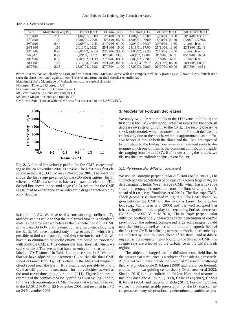
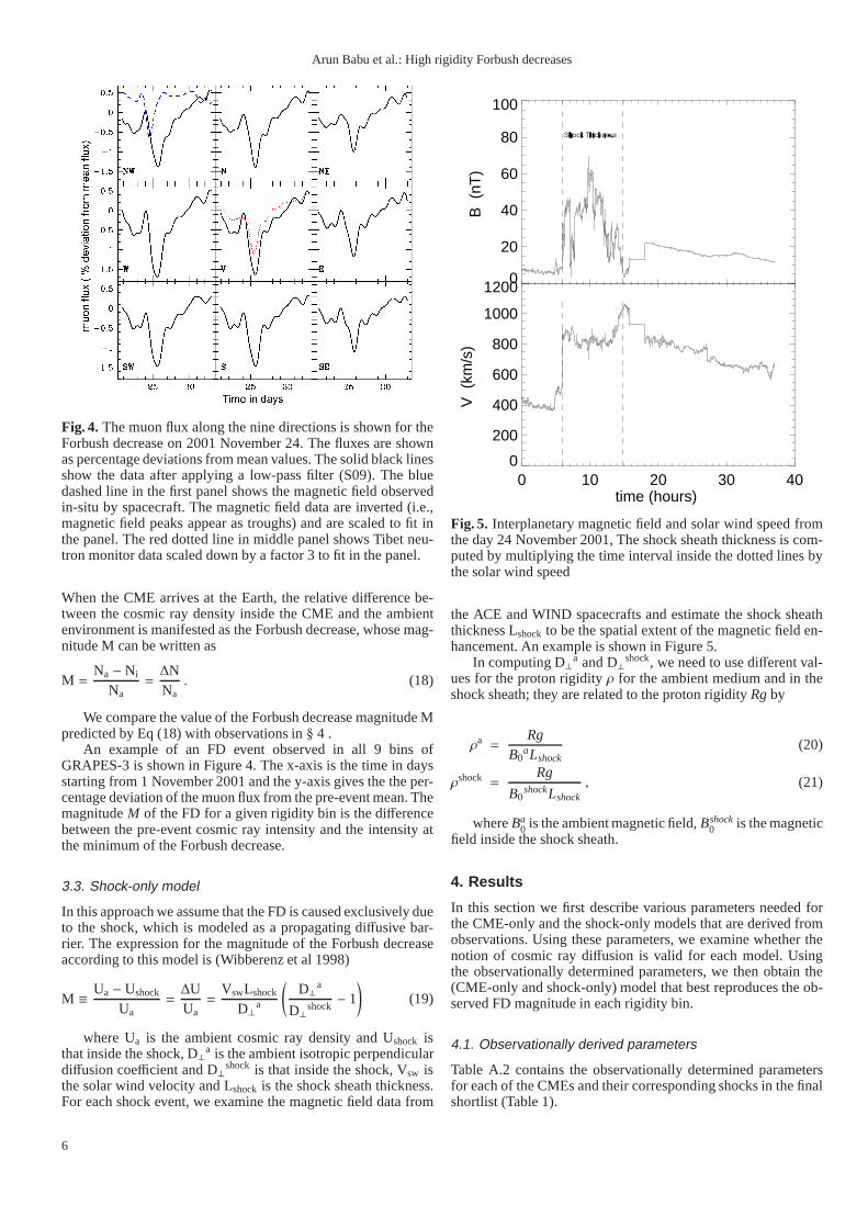
Fig. 4. The muon flux along the nine directions is shown for theForbush decrease on 2001 November 24. The fluxes are shownas percentage deviations from mean values. The solid black linesshow the data after applying a low-pass filter (S09). The bluedashed line in the first panel shows the magnetic field observedin-situ by spacecraft. The magnetic field data are inverted (i.e.,magnetic field peaks appear as troughs) and are scaled to fit inthe panel. The red dotted line in middle panel shows Tibet neu-tron monitor data scaled down by a factor 3 to fit in the panel.

When the CME arrives at the Earth, the relative difference be-tween the cosmic ray density inside the CME and the ambientenvironment is manifested as the Forbush decrease, whose mag-nitude M can be written as

M =Na− Ni

Na=∆NNa. (18)

We compare the value of the Forbush decrease magnitude Mpredicted by Eq (18) with observations in§ 4 .

An example of an FD event observed in all 9 bins ofGRAPES-3 is shown in Figure 4. The x-axis is the time in daysstarting from 1 November 2001 and the y-axis gives the the per-centage deviation of the muon flux from the pre-event mean. ThemagnitudeM of the FD for a given rigidity bin is the differencebetween the pre-event cosmic ray intensity and the intensity atthe minimum of the Forbush decrease.

3.3. Shock-only model

In this approach we assume that the FD is caused exclusively dueto the shock, which is modeled as a propagating diffusive bar-rier. The expression for the magnitude of the Forbush decreaseaccording to this model is (Wibberenz et al 1998)

M ≡Ua− Ushock

Ua=∆UUa=

VswLshock

D⊥a

(

D⊥a

D⊥shock− 1

)

(19)

where Ua is the ambient cosmic ray density and Ushock isthat inside the shock, D⊥a is the ambient isotropic perpendiculardiffusion coefficient and D⊥shock is that inside the shock, Vsw isthe solar wind velocity and Lshock is the shock sheath thickness.For each shock event, we examine the magnetic field data from

0

20

40

60

80

100

B (

nT)

0 10 20 30 40time (hours)

0

200

400

600

800

1000

1200

V (

km/s

)

Fig. 5. Interplanetary magnetic field and solar wind speed fromthe day 24 November 2001, The shock sheath thickness is com-puted by multiplying the time interval inside the dotted lines bythe solar wind speed

the ACE and WIND spacecrafts and estimate the shock sheaththickness Lshock to be the spatial extent of the magnetic field en-hancement. An example is shown in Figure 5.

In computing D⊥a and D⊥shock, we need to use different val-ues for the proton rigidityρ for the ambient medium and in theshock sheath; they are related to the proton rigidityRg by

ρa =Rg

B0aLshock

(20)

ρshock =Rg

B0shockLshock

, (21)

whereBa0 is the ambient magnetic field,Bshock

0 is the magneticfield inside the shock sheath.

4. Results

In this section we first describe various parameters needed forthe CME-only and the shock-only models that are derived fromobservations. Using these parameters, we examine whether thenotion of cosmic ray diffusion is valid for each model. Usingthe observationally determined parameters, we then obtainthe(CME-only and shock-only) model that best reproduces the ob-served FD magnitude in each rigidity bin.

4.1. Observationally derived parameters

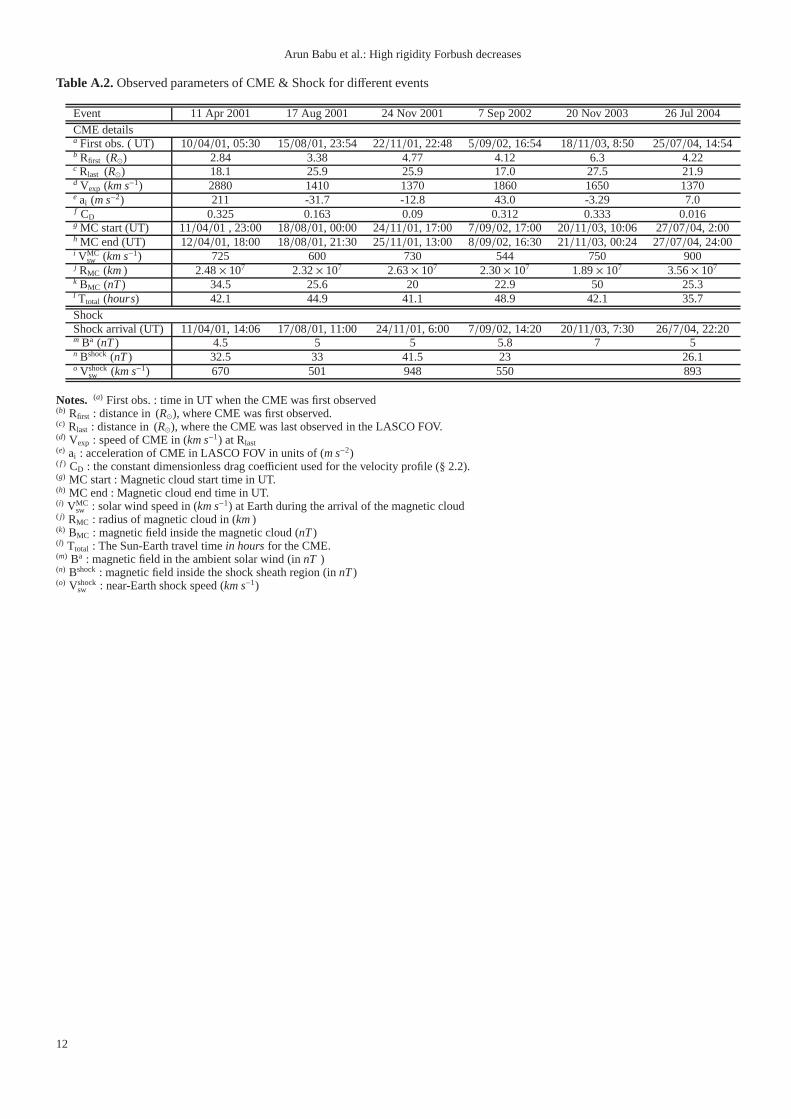
Table A.2 contains the observationally determined parametersfor each of the CMEs and their corresponding shocks in the finalshortlist (Table 1).

6

Arun Babu et al.: High rigidity Forbush decreases

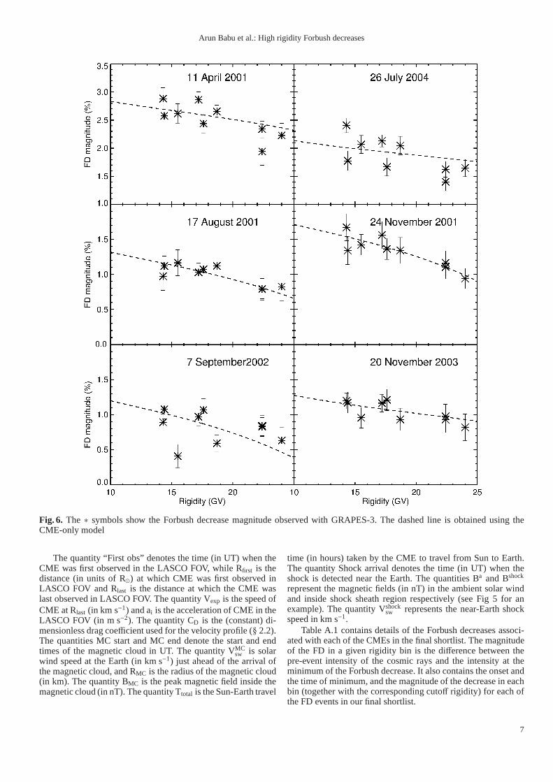
Fig. 6. The ∗ symbols show the Forbush decrease magnitude observed with GRAPES-3. The dashed line is obtained using theCME-only model

The quantity “First obs” denotes the time (in UT) when theCME was first observed in the LASCO FOV, while Rfirst is thedistance (in units of R⊙) at which CME was first observed inLASCO FOV and Rlast is the distance at which the CME waslast observed in LASCO FOV. The quantity Vexp is the speed ofCME at Rlast (in km s−1) and ai is the acceleration of CME in theLASCO FOV (in m s−2). The quantity CD is the (constant) di-mensionless drag coefficient used for the velocity profile (§ 2.2).The quantities MC start and MC end denote the start and endtimes of the magnetic cloud in UT. The quantity VMC

sw is solarwind speed at the Earth (in km s−1) just ahead of the arrival ofthe magnetic cloud, and RMC is the radius of the magnetic cloud(in km). The quantity BMC is the peak magnetic field inside themagnetic cloud (in nT). The quantity Ttotal is the Sun-Earth travel

time (in hours) taken by the CME to travel from Sun to Earth.The quantity Shock arrival denotes the time (in UT) when theshock is detected near the Earth. The quantities Ba and Bshock

represent the magnetic fields (in nT) in the ambient solar windand inside shock sheath region respectively (see Fig 5 for anexample). The quantity Vshock

sw represents the near-Earth shockspeed in km s−1.

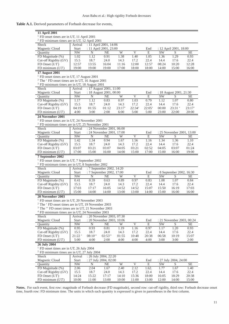
Table A.1 contains details of the Forbush decreases associ-ated with each of the CMEs in the final shortlist. The magnitudeof the FD in a given rigidity bin is the difference between thepre-event intensity of the cosmic rays and the intensity at theminimum of the Forbush decrease. It also contains the onset andthe time of minimum, and the magnitude of the decrease in eachbin (together with the corresponding cutoff rigidity) for each ofthe FD events in our final shortlist.

7

Arun Babu et al.: High rigidity Forbush decreases

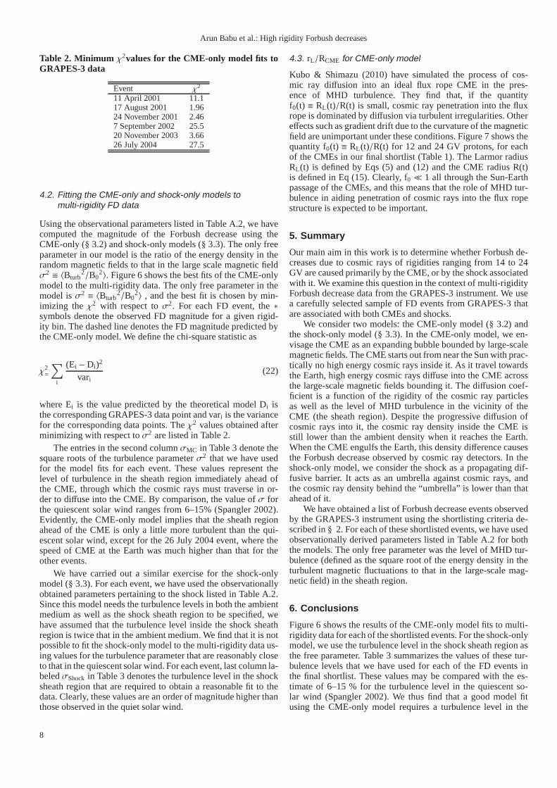
Table 2. Minimum χ2values for the CME-only model fits toGRAPES-3 data

Event χ2

11 April 2001 11.117 August 2001 1.9624 November 2001 2.467 September 2002 25.520 November 2003 3.6626 July 2004 27.5

4.2. Fitting the CME-only and shock-only models tomulti-rigidity FD data

Using the observational parameters listed in Table A.2, we havecomputed the magnitude of the Forbush decrease using theCME-only (§ 3.2) and shock-only models (§ 3.3). The only freeparameter in our model is the ratio of the energy density in therandom magnetic fields to that in the large scale magnetic fieldσ2 ≡ 〈Bturb

2/B02〉. Figure 6 shows the best fits of the CME-only

model to the multi-rigidity data. The only free parameter inthemodel isσ2 ≡ 〈Bturb

2/B02〉 , and the best fit is chosen by min-

imizing the χ2 with respect toσ2. For each FD event, the∗symbols denote the observed FD magnitude for a given rigid-ity bin. The dashed line denotes the FD magnitude predicted bythe CME-only model. We define the chi-square statistic as

χ2=

∑

i

(Ei − Di)2

vari(22)

where Ei is the value predicted by the theoretical model Di isthe corresponding GRAPES-3 data point and vari is the variancefor the corresponding data points. Theχ2 values obtained afterminimizing with respect toσ2 are listed in Table 2.

The entries in the second columnσMC in Table 3 denote thesquare roots of the turbulence parameterσ2 that we have usedfor the model fits for each event. These values represent thelevel of turbulence in the sheath region immediately ahead ofthe CME, through which the cosmic rays must traverse in or-der to diffuse into the CME. By comparison, the value ofσ forthe quiescent solar wind ranges from 6–15% (Spangler 2002).Evidently, the CME-only model implies that the sheath regionahead of the CME is only a little more turbulent than the qui-escent solar wind, except for the 26 July 2004 event, where thespeed of CME at the Earth was much higher than that for theother events.

We have carried out a similar exercise for the shock-onlymodel (§ 3.3). For each event, we have used the observationallyobtained parameters pertaining to the shock listed in TableA.2.Since this model needs the turbulence levels in both the ambientmedium as well as the shock sheath region to be specified, wehave assumed that the turbulence level inside the shock sheathregion is twice that in the ambient medium. We find that it is notpossible to fit the shock-only model to the multi-rigidity data us-ing values for the turbulence parameter that are reasonablycloseto that in the quiescent solar wind. For each event, last column la-beledσShock in Table 3 denotes the turbulence level in the shocksheath region that are required to obtain a reasonable fit to thedata. Clearly, these values are an order of magnitude higherthanthose observed in the quiet solar wind.

4.3. rL/RCME for CME-only model

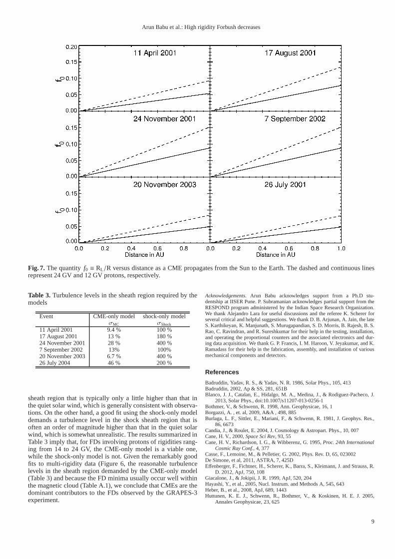
Kubo & Shimazu (2010) have simulated the process of cos-mic ray diffusion into an ideal flux rope CME in the pres-ence of MHD turbulence. They find that, if the quantityf0(t) ≡ RL(t)/R(t) is small, cosmic ray penetration into the fluxrope is dominated by diffusion via turbulent irregularities. Othereffects such as gradient drift due to the curvature of the magneticfield are unimportant under these conditions. Figure 7 showsthequantity f0(t) ≡ RL(t)/R(t) for 12 and 24 GV protons, for eachof the CMEs in our final shortlist (Table 1). The Larmor radiusRL(t) is defined by Eqs (5) and (12) and the CME radius R(t)is defined in Eq (15). Clearly, f0 ≪ 1 all through the Sun-Earthpassage of the CMEs, and this means that the role of MHD tur-bulence in aiding penetration of cosmic rays into the flux ropestructure is expected to be important.

5. Summary

Our main aim in this work is to determine whether Forbush de-creases due to cosmic rays of rigidities ranging from 14 to 24GV are caused primarily by the CME, or by the shock associatedwith it. We examine this question in the context of multi-rigidityForbush decrease data from the GRAPES-3 instrument. We usea carefully selected sample of FD events from GRAPES-3 thatare associated with both CMEs and shocks.

We consider two models: the CME-only model (§ 3.2) andthe shock-only model (§ 3.3). In the CME-only model, we en-visage the CME as an expanding bubble bounded by large-scalemagnetic fields. The CME starts out from near the Sun with prac-tically no high energy cosmic rays inside it. As it travel towardsthe Earth, high energy cosmic rays diffuse into the CME acrossthe large-scale magnetic fields bounding it. The diffusion coef-ficient is a function of the rigidity of the cosmic ray particlesas well as the level of MHD turbulence in the vicinity of theCME (the sheath region). Despite the progressive diffusion ofcosmic rays into it, the cosmic ray density inside the CME isstill lower than the ambient density when it reaches the Earth.When the CME engulfs the Earth, this density difference causesthe Forbush decrease observed by cosmic ray detectors. In theshock-only model, we consider the shock as a propagating dif-fusive barrier. It acts as an umbrella against cosmic rays, andthe cosmic ray density behind the “umbrella” is lower than thatahead of it.

We have obtained a list of Forbush decrease events observedby the GRAPES-3 instrument using the shortlisting criteriade-scribed in§ 2. For each of these shortlisted events, we have usedobservationally derived parameters listed in Table A.2 forboththe models. The only free parameter was the level of MHD tur-bulence (defined as the square root of the energy density in theturbulent magnetic fluctuations to that in the large-scale mag-netic field) in the sheath region.

6. Conclusions

Figure 6 shows the results of the CME-only model fits to multi-rigidity data for each of the shortlisted events. For the shock-onlymodel, we use the turbulence level in the shock sheath regionasthe free parameter. Table 3 summarizes the values of these tur-bulence levels that we have used for each of the FD events inthe final shortlist. These values may be compared with the es-timate of 6–15 % for the turbulence level in the quiescent so-lar wind (Spangler 2002). We thus find that a good model fitusing the CME-only model requires a turbulence level in the

8

Arun Babu et al.: High rigidity Forbush decreases

Fig. 7. The quantityf0 ≡ RL/R versus distance as a CME propagates from the Sun to the Earth. The dashed and continuous linesrepresent 24 GV and 12 GV protons, respectively.

Table 3. Turbulence levels in the sheath region required by themodels

Event CME-only model shock-only modelσMC σShock

11 April 2001 9.4 % 100 %17 August 2001 13 % 180 %24 November 2001 28 % 400 %7 September 2002 13% 100%20 November 2003 6.7 % 400 %26 July 2004 46 % 200 %

sheath region that is typically only a little higher than that inthe quiet solar wind, which is generally consistent with observa-tions. On the other hand, a good fit using the shock-only modeldemands a turbulence level in the shock sheath region that isoften an order of magnitude higher than that in the quiet solarwind, which is somewhat unrealistic. The results summarized inTable 3 imply that, for FDs involving protons of rigidities rang-ing from 14 to 24 GV, the CME-only model is a viable one,while the shock-only model is not. Given the remarkably goodfits to multi-rigidity data (Figure 6, the reasonable turbulencelevels in the sheath region demanded by the CME-only model(Table 3) and because the FD minima usually occur well withinthe magnetic cloud (Table A.1), we conclude that CMEs are thedominant contributors to the FDs observed by the GRAPES-3experiment.

Acknowledgements. Arun Babu acknowledges support from a Ph.D stu-dentship at IISER Pune. P. Subramanian acknowledges partial support from theRESPOND program administered by the Indian Space Research Organization.We thank Alejandro Lara for useful discussions and the referee K. Scherer forseveral critical and helpful suggestions. We thank D. B. Arjunan, A. Jain, the lateS. Karthikeyan, K. Manjunath, S. Murugapandian, S. D. Morris, B. Rajesh, B. S.Rao, C. Ravindran, and R. Sureshkumar for their help in the testing, installation,and operating the proportional counters and the associatedelectronics and dur-ing data acquisition. We thank G. P. Francis, I. M. Haroon, V.Jeyakumar, and K.Ramadass for their help in the fabrication, assembly, and installation of variousmechanical components and detectors.

References

Badruddin, Yadav, R. S., & Yadav, N. R. 1986, Solar Phys., 105, 413Badruddin, 2002, Ap & SS, 281, 651BBlanco, J. J., Catalan, E., Hidalgo, M. A., Medina, J., & Rodiguez-Pacheco, J.

2013, Solar Phys., doi:10.1007/s11207-013-0256-1Bothmer, V., & Schwenn, R. 1998, Ann. Geophysicae, 16, 1Borgazzi, A. , et. al, 2009, A&A , 498, 885Burlaga, L. F., Sittler, E., Mariani, F., & Schwenn, R. 1981,J. Geophys. Res.,

86, 6673Candia, J., & Roulet, E. 2004, J. Cosmology & Astropart. Phys., 10, 007Cane, H. V., 2000,Space Sci Rev, 93, 55Cane, H. V., Richardson, I. G., & Wibberenz, G. 1995,Proc. 24th International

Cosmic Ray Conf., 4, 377Casse, F., Lemoine, M., & Pelletier, G. 2002, Phys. Rev. D, 65, 023002De Simone, et al, 2011, ASTRA, 7, 425DEffenberger, F., Fichtner, H., Scherer, K., Barra, S., Kleimann, J. and Strauss, R.

D. 2012, ApJ, 750, 108Giacalone, J., & Jokipii, J. R. 1999, ApJ, 520, 204Hayashi, Y., et al., 2005, Nucl. Instrum. and Methods A, 545,643Heber, B., et al., 2008, ApJ, 689, 1443Huttunen, K. E. J., Schwenn, R., Bothmer, V., & Koskinen, H. E. J. 2005,

Annales Geophysicae, 23, 625

9

Arun Babu et al.: High rigidity Forbush decreases

Kubo, Y., & Shimazu, H. , 2010, ApJ, 720, 853Kuwabara, T., et al., 2009, JGRA, 114, 05109Lara, A., Flandes, A., Borgazzi, A., & Subramanian, P. 2011,J. Geophys. Res.,

116, CiteID A12102Leblanc, Y., et. al, 1998, Solar Phys., 183, 165Lockwood, J. A., Webber, W. R., & Debrunner, H. 1991, J. Geophys. Res., 96,

11587Lynch, B. J., Zurbuchen, T. H., Fisk, L. A., & Antiochos, S. K.2003, J. Geophys.

Res., 108, 1239Manoharan, P. K., et al., 2000, ApJ, 530, 1061Matthaeus et al, 2003, ApJ, 590L, 53MNonaka, T., et al., 2006, Phys. Rev. D, 74, 052003Oh, S. Y., Yi, Y., 2012, Solar Phys., 280, 197OPoomvises, W., Zhang, J., Olmedo, O., 2010, ApJ, 717L, 159PReames, D. V., Kahler, S. W., & Tylka, A. J. 2009, ApJ, 700, 196Richardson, I. G.& Cane , H. V. 2011, Solar Phys.,270, 609Sanderson, T. R., et al., 1990, Proc. 21st Int. Cosmic Ray Conf. 6, 251Shalchi, A., 2010, ApJ, 720L, 127SSchwenn, R., Dal Lago, A., Huttunen, E., & Gonzalez, W. D. 2005, Annales

Geophysicae, 23, 1033Spangler, S. R. 2002, ApJ, 576, 997Subramanian, P., & Vourlidas, A. 2007, A&A, 467, 685Subramanian, P., et. al 2009, A& A, 494, 1107Tautz, R. C., Shalchi, A. 2011, ApJ, 735, 92Vourlidas, A., Lynch, B. J., Howard, R. A., & Li, Y. 2012, Solar Phys, tmp, 192V.

DOI: 10.1007/s11207-012-0084-8Wang Y., Zhou, G., Ye, P., Wang, S., & Wang, J. 2006, ApJ, 651, 1245Wibberenz, G., le Roux, J. A., Potgieter, M. S., & Bieber, J. W. 1998, Space Sci.

Rev., 83, 309Yu, X. X., Lu , H., Le, G. M., & Shi, F., 2010, Solar Phys, 263, 223Zhang, G., & Burlaga, L. F. 1988, J. Geophys. Res., 93, 2511

Appendix A: Tables

10

Arun Babu et al.: High rigidity Forbush decreases

Table A.1.Derived parameters of Forbush decrease for events,

11 April 20011 FD onset times are in UT, 11 April 20012 FD minimum times are in UT, 12 April 2001Shock Arrival : 11 April 2001, 14:06Magnetic Cloud Start : 11 April 2001, 23:00 End : 12 April 2001, 18:00Quantity NW N NE W V E SW S SEFD Magnitude (%) 1.02 1.12 0.91 1.38 1.40 1.05 1.36 1.29 0.93Cut-off Rigidity (GV) 15.5 18.7 24.0 14.3 17.2 22.4 14.4 17.6 22.4FD Onset (UT ) 12:57 13:55 16:04 11:16 12:00 12:57 08:24 10:20 12:28FD minimum (UT ) 19:00 19:00 19:00 17:00 18:00 18:00 14:00 15:00 16:0017 August 20011 FD onset times are in UT, 17 August 20012 The∗ FD onset times are in UT, 16 August 20013 FD minimum times are in UT, 18 August 2001Shock Arrival : 17 August 2001, 11:00Magnetic Cloud Start : 18 August 2001, 00:00 End : 18 August 2001, 21:30Quantity NW N NE W V E SW S SEFD Magnitude (%) 1.17 1.12 0.83 0.97 1.03 0.79 1.12 1.07 0.80Cut-off Rigidity (GV) 15.5 18.7 24.0 14.3 17.2 22.4 14.4 17.6 22.4FD Onset (UT ) 04:19 01:55 01:12 23:17∗ 22:34∗ 22:05∗ 00:00 23:31∗ 23:17∗

FD minimum (UT ) 4:00 3:00 2:00 6:00 5:00 5:00 23:00 22:00 20:0024 November 20011 FD onset times are in UT, 24 November 20012 FD minimum times are in UT, 25 November 2001Shock Arrival : 24 November 2001, 06:00Magnetic Cloud Start : 24 November 2001, 17:00 End : 25 November 2001, 13:00Quantity NW N NE W V E SW S SEFD Magnitude (%) 1.42 1.34 0.94 1.67 1.56 1.16 1.34 1.36 1.10Cut-off Rigidity (GV) 15.5 18.7 24.0 14.3 17.2 22.4 14.4 17.6 22.4FD Onset (UT ) 03:07 03:21 03:07 04:05 03:21 02:52 04:05 03:07 01:24FD minimum (UT ) 17:00 15:00 16:00 14:00 15:00 17:00 15:00 16:00 19:007 September 20021 FD onset times are in UT, 7 September 20022 FD minimum times are in UT, 8 September 2002Shock Arrival : 7 September 2002, 14:20Magnetic Cloud Start : 7 September 2002, 17:00 End : 8 September 2002, 16:30Quantity NW N NE W V E SW S SEFD Magnitude (%) 0.41 0.59 0.63 0.89 0.97 0.83 1.08 1.07 0.84Cut-off Rigidity (GV) 15.5 18.7 24.0 14.3 17.2 22.4 14.4 17.6 22.4FD Onset (UT ) 17:03 17:17 16:05 14:52 14:52 15:07 15:50 16:19 17:03FD minimum (UT ) 15:00 14:00 14:00 13:00 13:00 14:00 15:00 16:00 16:0020 November 20031 FD onset times are in UT, 20 November 20032 The∗ FD onset times are in UT, 19 November 20033 The∗∗ FD onset times are in UT, 21 November 20034 FD minimum times are in UT, 24 November 2003Shock Arrival : 20 November 2003, 07:30Magnetic Cloud Start : 20 November 2003, 10:06 End : 21 November 2003, 00:24Quantity NW N NE W V E SW S SEFD Magnitude (%) 0.95 0.93 0.81 1.19 1.16 0.97 1.17 1.20 0.93Cut-off Rigidity (GV) 15.5 18.7 24.0 14.3 17.2 22.4 14.4 17.6 22.4FD Onset (UT ) 21:22∗ 08:10∗∗ 02:53∗∗ 01:55 10:48 20:38 06:58 10:19 15:07FD minimum (UT ) 5:00 4:00 2:00 4:00 4:00 4:00 3:00 3:00 2:0026 July 20041 FD onset times are in UT, 26 July 20042 FD minimum times are in UT, 27 July 2004Shock Arrival : 26 July 2004, 22:20Magnetic Cloud Start : 27 July 2004, 02:00 End : 27 July 2004, 24:00Quantity NW N NE W V E SW S SEFD Magnitude (%) 2.06 2.04 1.67 2.40 2.12 1.62. 1.77 1.67 1.40Cut-off Rigidity (GV) 15.5 18.7 24.0 14.3 17.2 22.4 14.4 17.6 22.4FD Onset (UT ) 14:24 15:22 17:17 14:10 15:36 18:00 16:05 18:29 20:38FD minimum (UT ) 10:00 11:00 13:00 10:00 11:00 13:00 12:00 14:00 15:00

Notes. For each event, first row: magnitude of Forbush decrease (FD magnitude), second row: cut-off rigidity, third row: Forbush decrease onsettime, fourth row: FD minimum time. The units in which each quantity is expressed is given in parentheses in the first column.

11

Arun Babu et al.: High rigidity Forbush decreases

Table A.2.Observed parameters of CME & Shock for different events

Event 11 Apr 2001 17 Aug 2001 24 Nov 2001 7 Sep 2002 20 Nov 2003 26 Jul 2004CME detailsa First obs. ( UT) 10/04/01, 05:30 15/08/01, 23:54 22/11/01, 22:48 5/09/02, 16:54 18/11/03, 8:50 25/07/04, 14:54b Rfirst (R⊙) 2.84 3.38 4.77 4.12 6.3 4.22c Rlast (R⊙) 18.1 25.9 25.9 17.0 27.5 21.9d Vexp (km s−1) 2880 1410 1370 1860 1650 1370e ai (m s−2) 211 -31.7 -12.8 43.0 -3.29 7.0f CD 0.325 0.163 0.09 0.312 0.333 0.016g MC start (UT) 11/04/01 , 23:00 18/08/01, 00:00 24/11/01, 17:00 7/09/02, 17:00 20/11/03, 10:06 27/07/04, 2:00h MC end (UT) 12/04/01, 18:00 18/08/01, 21:30 25/11/01, 13:00 8/09/02, 16:30 21/11/03, 00:24 27/07/04, 24:00i VMC

sw (km s−1) 725 600 730 544 750 900j RMC (km ) 2.48× 107 2.32× 107 2.63× 107 2.30× 107 1.89× 107 3.56× 107

k BMC (nT ) 34.5 25.6 20 22.9 50 25.3l Ttotal (hours) 42.1 44.9 41.1 48.9 42.1 35.7ShockShock arrival (UT) 11/04/01, 14:06 17/08/01, 11:00 24/11/01, 6:00 7/09/02, 14:20 20/11/03, 7:30 26/7/04, 22:20m Ba (nT ) 4.5 5 5 5.8 7 5n Bshock (nT ) 32.5 33 41.5 23 26.1o Vshock

sw (km s−1) 670 501 948 550 893

Notes. (a) First obs. : time in UT when the CME was first observed(b) Rfirst : distance in (R⊙), where CME was first observed.(c) Rlast : distance in (R⊙), where the CME was last observed in the LASCO FOV.(d) Vexp : speed of CME in (km s−1) at Rlast(e) ai : acceleration of CME in LASCO FOV in units of (m s−2)( f ) CD : the constant dimensionless drag coefficient used for the velocity profile (§ 2.2).(g) MC start : Magnetic cloud start time in UT.(h) MC end : Magnetic cloud end time in UT.(i) VMC

sw : solar wind speed in (km s−1) at Earth during the arrival of the magnetic cloud( j) RMC : radius of magnetic cloud in (km )(k) BMC : magnetic field inside the magnetic cloud (nT )(l) Ttotal : The Sun-Earth travel timein hours for the CME.(m) Ba : magnetic field in the ambient solar wind (innT )(n) Bshock : magnetic field inside the shock sheath region (innT )(o) Vshock

sw : near-Earth shock speed (km s−1)

12