Teacher Shocks and Student Learning:

Evidence from Zambia.∗

Jishnu Das (The World Bank) Stefan Dercon (Oxford University)James Habyarimana (Georgetown University)Pramila Krishnan (Cambridge University)

April 26, 2005

Abstract

A large literature examines the link between shocks to households and the educational at-

tainment of children.We use new data to estimate the impact of shocks to teachers on studentlearning in Mathematics and English. Using absenteeism in the 30 days preceding the survey as

a measure of these shocks we find large impacts: A 5-percent increase in the teacher’s absence

rate reduces learning by 4 to 8 percent of average gains over the year. This reduction in learning

achievement likely reflects both the direct effect of increased absenteeism and the indirect effects

of less lesson preparation and lower teaching quality when in class. We document that health

problems–primarily teachers’ own illness and the illnesses of their family members—accountfor more than 60 percent of teacher absences; not surprising in a country struggling with an

HIV/AIDS epidemic. The relationship between shocks to teachers and student learning suggests

that households are unable to substitute adequately for teaching inputs. Excess teaching ca-

pacity that allows for the greater use of substitute teachers could lead to larger gains in student

learning.

∗Corresponding Author: James Habyarimana (jph35@georgetown.edu). We thank workshop participants at theHarvard, Oxford, University College London, CEMFI (Madrid) and Indiana (Purdue) for useful comments andsuggestions. Funding for the survey was provided by DFID. The Policy Research Working Paper Series disseminatesthe findings of work in progress to encourage the exchange of ideas about development issues. An objective of theseries is to get the findings out quickly, even if the presentations are less than fully polished. The papers carrythe names of the authors and should be cited accordingly. The findings, interpretations, and conclusions expressedin this paper are entirely those of the authors. They do not necessarily represent the view of the World Bank,its Executive Directors, or the countries they represent. Policy Research Working Papers are available online athttp://econ.worldbank.org.

1

Pub

lic D

iscl

osur

e A

utho

rized

Pub

lic D

iscl

osur

e A

utho

rized

Pub

lic D

iscl

osur

e A

utho

rized

Pub

lic D

iscl

osur

e A

utho

rized

Pub

lic D

iscl

osur

e A

utho

rized

Pub

lic D

iscl

osur

e A

utho

rized

Pub

lic D

iscl

osur

e A

utho

rized

Pub

lic D

iscl

osur

e A

utho

rized

1 Introduction

The relationship between schooling inputs and educational outcomes continues to receive wide

attention in discussions about how to improve educational outcomes. Educational investment,

particularly in poor countries, depends a good deal on publicly provided resources to schools.

However, it is also influenced by inputs at the household level. For some resources, such as textbooks

and other educational materials, parents are able to substitute at home what is not provided in the

school. For other resources, such substitution may be harder.

Consensus is building that teachers constitute a school-level resource that parents find hard to

substitute for at home. It is possible that parents do not have the time or skills to teach their

children at home. Further, the agency costs of hiring teachers in a market may be high and such

costs may be accentuated due to low overall levels of learning in low-income countries. Perhaps not

surprisingly then, the literature consistently finds that teachers contribute significantly to levels

and growth in learning achievement; however, considerable debate continues about the specific

attributes of teachers that matter.

A key problem has been identification; in particular, it is hard to separate the effects of house-

hold resources from school inputs on learning achievement. Parallel work on the contribution of

households focus on how household-level shocks affect educational attainment (two examples are

Jacoby and Skoufias 1997; de Janvry and others 2005). To our knowledge though, there has been

little work on how school-level shocks might affect learning achievement, even though it provides a

means of identifying the impact of school resources.

We address this gap by examining the effect of shocks that teachers faced on student learning.

The study focuses on Zambia, where the impact of AIDS and other illnesses seem to be the reason

for much of the observed absenteeism of teachers.1 The paper isolates the effect of the shocks

that teachers face during an academic year–primarily their own illness and the illnesses of family

members–on student learning. These shocks, as measured by episodes of teacher absence, led to

large losses in learning achievement. A shock associated with a 5 percent increase in teacher absence

reduced learning achievement by 4 to 8 percent of average gains in English and Mathematics during

the academic year studied. The size of the estimated impact is substantial and, in addition to the

losses due to time away from class, probably reflects lower teaching quality when in class and less

lesson preparation when at home.

1This is in marked contrast to say, India, where incentives to teachers to perform well seem to be the reason forabsenteeism and hence the nature of the problem and its impact are considerably different.

2

The impact is robust to controls for student absenteeism. The estimated impact of student

absenteeism is of the same magnitude as the effect of shocks to teachers. Since every teacher teaches

many students, this raises the possibility that excess teaching capacity, which allows for the greater

use of substitute teachers, could significantly increase learning achievement. The protective effect

of such insurance could have larger impacts on learning achievement than insuring and supporting

students and their families. Moreover, in countries with a high HIV/AIDS burden, substantial

welfare gains could accrue through a reduction in the frequency or impact of shocks associated

with absenteeism. For example, Bell, Devarajan and Gersbach (2003) posit huge declines in human

capital due to the effects of the HIV/AIDS epidemic on affected economies. The results presented

in this paper provide strong micro-foundations for this assumption and challenge conclusions that

find a small (or no) impact of the HIV epidemic on the education sector (Bennell 2005).

To contextualize our empirical results, we present a model where households determine the

optimal path of educational attainment given teacher and other school inputs (Das and others 2004).

In this framework, teachers possess three attributes—observable characteristics (age, gender and

experience), unobserved non-time varying attributes (such as ability or motivation) and unobserved

time varying attributes (such as the health status). As households try to optimize over future time

periods, they face uncertainty related to two school-based inputs: uncertainty in the quality of the

teacher (non-time varying) and timing and severity of shocks to the teacher (time-varying).

The model shows how variation in the non-time varying and time-varying attributes affect learn-

ing achievement. It thus allows us to advance the prominent role of households in determining their

children’s cognitive achievement. In addition, it clarifies the identification assumptions required to

estimate the impact of teacher-level shocks on student learning. In particular, one contribution

is to show that the impact of teacher-level shocks on learning is identified only if non-time vary-

ing heterogeneity for both students and teachers is adequately dealt with through the estimation

procedure.

The empirical results are based on a rich teacher-student matched data set from Zambia that

we collected in 2002. In addition to school, teacher, and student characteristics, the data include

test scores for a sample of pupils over two years. This panel of test scores allows us to deal with

omitted variable bias associated with student tracking, but does not account for unobserved changes

in teacher characteristics. To do so, we exploit a tradition in which some teachers stay with the

same student cohort throughout primary school. By restricting attention to the sample of pupils

with the same teacher in both years, and this is the basis of our identification strategy, we address

concerns that arise from unobserved child and teacher heterogeneity.

3

For students who remained with the same teacher, there is a large and significant effect of

negative shocks to the teacher on learning. This result is robust across specifications. It is also

robust to a number of identification problems common to estimating the impact of school inputs

on learning, which we discuss below. However, the results obtained on the sample of students who

remained with the same teacher do not extend to those who switched teachers during the two years

of the study. We suggest two reasons for this finding. The first is selective matching of students

and teachers, and the second is higher precautionary educational spending among households whose

children switched teachers. Although we are able to show that the differential impact among the

movers and non-movers did not arise from differences in the sample of students, we are unable to

distinguish between these two suggested channels.

The remainder of the paper is organized as follows. Section 2 reviews the literature. Section

3 outlines the theory. Section 4 presents the empirical specification and econometric concerns.

Section 5 discusses the data used and section 6 presents the results and robustness tests for the

sample of children who stayed with the same teacher. Section 7 focuses on the sample of children

who switched teachers and section 8 concludes with some caveats and a discussion of the policy

implications.

2 Literature Review

Interest in teacher attributes on student learning has recently emerged in the educational production

function literature. Papers using analysis of variance techniques have shown that the variation in

test scores explained by teachers is substantial. Hanushek, Kain and Rivkin (1998), using data

from Tennessee schools, find evidence of significant teacher effects. Park and Hannum (2002),

using student-teacher matched data from China, find that variation due to teacher effects explains

about 25 percent of variation in test scores. More traditional regression-based studies also validate

this finding. Rockoff (2004) using a 12-year panel of teacher-student data from two school districts

in New Jersey finds significant teacher fixed effects. A one standard deviation change in the teacher

fixed effect (unobserved quality) is associated with gains in Mathematics and reading of 0.26 and

0.16 standard deviations respectively. Less is known about the specific attributes of teachers that

affect student learning. Limited evidence on teacher experience and training is provided by Rockoff

(2004) and Angrist and Lavy (2001), who find that both experience and training have a positive

impact on learning achievement.

Closer to the results presented here are the studies by Jacobson (1989) and Ehrenberg and

others (1991). Jacobson (1989) describes an interesting policy experiment in which a pot of money

4

was set aside and teachers’ claims on the pot were proportional to sick leave days not taken. This

policy reduced the number of sick days taken by 30 percent and increased the share of teachers

with perfect attendance from 8 percent to 34 percent.2 Data was not available to evaluate the

impact of this policy on student performance. Ehrenberg and others (1991) study the effect of

teacher absenteeism on school level pass-rates using variation in school district leave policies as an

instrument for absenteeism. They find no direct effects of absenteeism on pass-rates, although they

do find that higher teacher absenteeism is associated with higher student absenteeism.

Our paper focuses on identifying the impact of negative shocks on learning achievement using

absenteeism as a plausible measure of shocks rather than the impact of absenteeism per se. Negative

shocks that result in higher absenteeism may also lead to less supplementary inputs by the teacher.

A teacher who is sick is likely to be absent more often and also likely to spend less time on lesson

preparation. Our estimates thus capture the joint effect of absence from the classroom and lower

inputs due to the shock. The policy implications (discussed below) vary accordingly.

The institutional context presents another source of difference. It is likely that the nature

and severity of shocks that teachers experience varies dramatically across the United States and

low-income countries. In a country like Zambia, with very high HIV prevalence, shocks due to

illnesses and funerals can lead to long absences and substantial declines in teaching performance.

The difference in absenteeism is striking. Absence rates in U.S.-based studies of 5 percent (or in

Jacobson’s case an average of 7 days per year) are low compared to those in low-income countries–

an ongoing study finds averages of 20 percent and above in Sub-Saharan Africa, 25 percent in India

and 11 percent and above in Latin America (Chaudhury and Hammer 2005; Chaudhury and others

2004; World Bank 2003; Glewwe and others 2001).3 In Zambia, the percentage of teachers absent

from school at the time of a surprise visit was closer to 18 percent and average days of absence

fall just under 21 days during the year.4 In addition, in the U.S. the policy of providing substitute

teachers minimizes disruption. Although evidence on teacher absenteeism in low income countries

is sparse, the use of substitute teachers is low. Thus, both the extent of shocks and the ability of

schools to cope is accentuated in our data.

Finally, the impact of teacher shocks is identified only for the sample of children who remained

with the same teacher over two years. For children who changed teachers between the first and the

second year of the study, heterogeneity in non-time varying teacher attributes such as motivation,2 Interestingly though, the courts decided not to implement the incentive scheme for a second year since it resulted

in a large number of "walking-wounded"–teachers who came into work despite being sick!3 In fact, even private sector absence in India at 10 percent is double that reported for public schools in the US.4Note that this one-time measure is unable to distinguish between teachers who are frequently absent from those

who are absent infrequently.

5

confounds the interpretation of the estimate. This requires data that matches specific students and

teachers, a requirement that is hard to fulfill in most countries; Ehrenberg and others (1991) for

instance use district level data, which could partially explain the lack of a relationship between

teacher absence and student learning in their study.

3 Theory

The model is based on Das and others (2004a). It is extended here to explicitly focus on the

implications of uncertainty in teacher inputs on household decisions about educational inputs and

cognitive achievement, as measured by test scores. The model assumes a household (with a sin-

gle child attending school) that derives (instantaneous) utility from the cognitive achievement of

the child TS and the consumption of other goods X. The household maximizes an intertemporal

utility function U(.), additive over time and states of the world with discount rate β(< 1) subject

to an intertemporal budget constraint (IBC) relating assets in the current period to assets in the

previous period, current expenditure and current income. Finally, cognitive achievement is deter-

mined by a production function relating current achievement (TSt) to past achievement (TSt−1),household educational inputs (zt), teacher inputs (mt), non-time varying child characteristics (µ)

and non time-varying teacher and school characteristics (η). We impose the following structure on

preferences and the production function for cognitive achievement:

[A1] Household utility is additively separable, increasing, and concave in cognitive achievement

and other goods.

[A2] The production function for cognitive achievement is given by TSt = F (TSt−1,mt, zt, µ, η)where F (.) is concave in its arguments.

Under [A1] and [A2] the household problem is

Max(Xt,zt) Uτ = Eτ

T

t=τ

βt−τ [u(TSt) + v(Xt)] s.t. (1)

At+1 = (1 + r).(At + yt − PtXt − zt) (2)

TSt = F (TSt−1,mt, zt, µt, η) (3)

AT+1 = 0 (4)

Here u and v are concave in each of its arguments. The intertemporal budget constraint (2) links

asset levels At+1 at t+1 with initial assets At, private spending on educational inputs zt, income ytand the consumption of other goods Xt. The price of educational inputs is the numeraire, the price

6

of other consumption goods is Pt, and r is the interest rate. The production function constraint (3)

dictates how inputs are converted to educational outcomes and the boundary condition (4) requires

that at t = T the household must have zero assets so that all loans are paid back and there is no

bequest motive.5

We assume that teacher inputs consist of two parts, and both are outside the control of the

household–inputs conditional on quality mqt and shocks to these inputs µt. The shocks are zero

in expectation (E(µt) = 0) so that mt = mqt + µt. Teacher inputs conditional on quality mqt are

assumed to be unknown, but at the time the household makes its decision it knows the underlying

distribution of quality and the stochastic process related to µt (but not the actual level). The two

sources of uncertainty in this model are uncertainty about the quality of teachers and uncertainty

about shocks to teacher inputs.

Maximization of (1) subject to (2) and (3) provides a decision rule related to TSt, characterizing

the demand for cognitive achievement. To arrive at this decision rule, we define a price for cognitive

achievement as the “user-cost” of increasing the stock in one period by one unit, i.e., the relevant

(shadow) price in each period for the household. This user-cost, evaluated at period t is (see Das

and others (2004a)):

πt =1

Fzt(.)− FTSt(.)

(1 + r)Fzt+1(.)(5)

The first term measures the cost of taking resources at t and transforming it into one extra mark in

the test. When implemented through a production function, the price is no longer constant–if the

production function is concave, the higher the initial levels of cognitive achievement, the greater the

cost of buying an extra unit as reflected in the marginal value, Fzt(.). Of the additional unit bought

in period t, the amount left to sell in period t+1 is FTSt(.) and the second term thus measures the

present value of how much of this one unit will be left in the next period expressed in monetary

terms. The standard first-order Euler condition related to the optimal path of educational outcomes

between period t and t+ 1 is then:

∂U∂TSt

πt= βEt

∂U∂TSt+1

πt+1(6)

5As discussed in Das et al. (2004a), an alternative assumption, that the benefits from the child’s cognitiveachievement are only felt in the future, would not change the model. Moreover, the results are unaffected if oneassumes that households care about the (instantaneous) flow from educational outcomes (rather than the stock ofcognitive achievement) provided that this flow is linear in the stock.

7

Intuitively this expression (ignoring uncertainty for the moment) suggests that if the user-cost of

test scores increases in one period t + 1 relative to t, along the optimal path this would increase

the marginal utility at t+1, so that TSt+1 will be lower. This is a standard Euler equation stating

that along the optimal path, cognitive achievement will be smooth, so that the marginal utilities of

educational outcomes will be equal in expectations, appropriately discounted and priced. Finally,

the concavity of the production function will limit the willingness of households to boost education

“too rapidly” since the cost is increasing in household inputs. Thus, under reasonable restrictions,

the optimal path will be characterized by a gradual increase in educational achievement over time

(for an explicit derivation see Deaton and Muellbauer 1980; and Foster 1995).

This general framework allows us to make predictions about the impact of information about

teacher quality and of shocks to teacher inputs. First, any shock in teacher inputs will affect the

path of test scores over time. Secondly, uncertainty ex ante about teacher quality may result in

fluctuations ex post in outcomes. For example, if at t+ 1 teacher quality is better than expected,

then households will have relatively overspent on educational inputs, boosting outcomes in t + 1

beyond the anticipated smooth path. It also implies that the (ex post observable) change in teacher

quality between t and t+1 matters for describing the change in outcomes and these changes should

be included in an empirical specification.

The uncertainty faced by households may also result in ex ante responses, affecting outcomes

as well as the impact of shocks on outcomes. To see this, consider the first-order condition affecting

choices between spending on educational inputs and on other goods before teacher quality is known.

The optimal decision rule equates the marginal utility of spending on other goods to the expected

value of spending on educational inputs (taking into account the intertemporal decision rule in (6)),

or:

∂U∂Xt

Pt= Et−1

∂U∂TSt

πt(7)

In general, whether increased risk in teacher quality will increase or reduce household spending

on educational inputs will depend on risk preferences and the nature and shape of the cognitive

production function. In particular, given Pt, if increasing risk increases the right-hand side of

equation (7), households will spend less on other goods Xt and more on teaching inputs zt than

before. Two implications emerge. First, the expected path of educational outcomes would be

higher–although this will not necessarily have an impact on the changes in outcomes between two

periods. Secondly, the ex post impact of shocks to teacher inputs in a particular period may be

8

different depending on the extent of risk faced by households ex ante.6

Appendix 2 develops the circumstances under which an increase in the ex-ante risk faced by

households leads to a decrease in the impact of ex post shocks due to a commensurate increase in

ex ante household investment. For the environment studied in this paper, this implies that the

sample of students who switched teachers (and thus faced greater uncertainty regarding teacher

quality) would be less susceptible to shocks in teacher inputs, for instance through the teacher’s or

her family’s ill health. Note that this difference in the estimated impact of the shock arises even

if movers are randomly assigned to teachers. Thus, to the extent the households increase their ex

ante educational investment due to precautionary motives, we expect to find a larger coefficient of

teacher-level shocks on student learning for children who stayed with the same teacher compared

to children who switched.7 8

4 Empirical Model and Identification

To derive an empirical specification, as in Das and others (2004), the following assumptions are

required.

[A1] Household utility is additively separable and of the CRRA form.

[A2] TSt = (1− δ)TSt−1 + F (wt, zt, µ, η) where the Hessian of F (.) is negative semi-definite.

Under assumption [A1] (6) can be written as:

TStTSt−1

−ρβπt−1πt

= 1 + et (8)

6Note that the latter possibility only arises due to the fact that households may influence educational outcomesvia their own inputs; if outcomes were only produced by teacher inputs, then there would be no difference in observedoutcomes conditional on the uncertainty faced by parents about teacher quality, since ex ante no actions could havebeen taken to avoid this.

7This result may at first seem counter intuitive: Producing cognitive achievement using household inputs is arisky activity. So, responding to increased risk by spending more on the risky activity may go against the basic resultsdiscussed in Sandmo (1969). However, since the produced commodity also enters the utility function, these resultsdo not hold, and under reasonable conditions, households may choose to invest more in the activity in response tomore uncertainty, as a means of guaranteeing a reasonable amount of the produced commodity for consumption.The argument is similar to the analysis of precautionary savings, where the choice is between consuming more todaycompared to tomorrow, as in Deaton (1992). In the basic model, convexity of marginal utility is then sufficient forincreased savings in response to increased uncertainty in income, even though the risk related to future utility hasincreased, affecting the marginal benefit to savings.

8 If the price of boosting cognitive achievement were constant, then convexity of marginal utility is sufficient. Ifnot, then as long as user-costs increase only at a decreasing rate in teacher inputs, households will still spend moreon household-level educational inputs when risk increases. In this formulation credit markets are perfect so thatthere are no bounds on At+1 apart from (4); the perfect credit market assumption is relaxed in our discussion of theempirical results. To see how the theory is affected, see Das et al. (2004a).

9

where et is an expectation error, uncorrelated with information at t−1. Taking logs, the expressionfor child i is:

lnTSitTSit−1

=1

ρlnβ − 1

ρln(

πitπit−1

) +1

ρln(1 + eit) (9)

or, the growth path is determined by the path of user-costs, and a term capturing expectational

surprises.

The key issue is how changes in the two types of teacher inputs mqt and µt impact the optimal

path of cognitive achievement. To provide a direct measure of the impact of shocks in teacher inputs

on the growth path of cognitive achievement, we add a direct measure of the shock in Equation

(9). If there is an (unanticipated) shock µt to teacher inputs ex post, then the change in the growth

path is given by ln(TSt−1+µtFmTSt−1 ), which depends on the relative size of the terms in brackets. In

light of the above, our empirical specification is given by:

lnTSijktTSijkt−1

= αo + α1µjkt + α2∆tjkt + α3∆Xjkt + {∆mqt + ijkt} (10)

where TSijkt is the test score of child i with teacher j in school k at time t; µjkt is a measure of a

shock to teacher inputs of teacher j in school k; ∆tjkt represents a vector of changes in observable

teacher characteristics and ∆Xjkt represents a vector of changes in other variables thought to affect

the relative user-cost of boosting cognitive achievement. The more negative is α1, the larger the

impact of shocks on test scores. Finally, the error term consists of changes to unobserved teacher

characteristics ∆mqt and a child-level shock ijkt.

4.1 Identification Among "Non-Movers"

The identification assumption implicit in Equation(10) is that cov(µjkt, {∆mqt +εijkt}) = 0, i.e, theerror term in the equation is not correlated with teacher-level shocks. Consider the non-movers

sample first. For this sample, ∆mqt = 0 so that α1 is identified if cov(µjkt, ijkt) = 0, i.e., teacher-

level shocks are orthogonal to student-level shocks. This assumption breaks down if, for instance,

the shocks that teachers are susceptible to are covariate with shocks that students face–a drought

in a village would likely affect both student and teachers equally, biasing our results away from

zero.

There is also an additional specification error if households are unable to substitute for teaching

inputs. In this case, unobserved teacher characteristics still have a persistent effect on student

performance and mqt will enter independently in the error term of Equation (10) above. While

the Euler model considered here explicitly rules out such persistence (for instance, through lagged-

10

stock adjustment), we discuss the robustness of our results to the omitted-variables and specification

errors below.

4.2 Identification Among "Movers"

For the sample of movers, an additional source of bias is introduced through selective matching.

Thus, if cov(∆mqt , µjkt) = 0, so that the change in unobserved teacher quality is correlated with

teacher-level shocks, then α1 captures both the effect of shocks and changes in teacher quality for

the movers. If children who changed teachers (movers) did so from very bad to bad teachers (so

that ∆mqt is positive), but these (unobservably) bad teachers are more absent than the average in

the sample, the covariance condition implies that our estimated impact for the movers is biased

towards zero. Note that there is a difference in interpretation between the selective matching and

the precautionary spending channel developed in the theory and appendix 2. For the latter, even

when cov(∆mqt , µjkt) = 0 so that there is no bias in the coefficient, the impact of teacher shocks is

still closer to zero for the sample of movers–this is due to heterogeneity in the treatment impact

and accordingly has different estimation implications.

Estimating the impact of teacher shocks requires data both on the extent of these shocks and a

means of distinguishing the uncertainty faced by households in terms of teacher inputs. The primary

measure of shocks to teacher inputs used in this paper is teacher absenteeism. As will be shown

below, this absenteeism arises from a number of factors, largely unpredictable for the households,

such as illness and attendance at funerals. We first estimate the impact of teacher shocks for the

non-movers and discuss the robustness of our results to the concerns raised above. We then show

that the results do not extend to the sample of movers. We are unable, however, to distinguish

between the selective matching (which results in a bias in the estimates) and precautionary spending

(which results in heterogeneity in the impact of teacher shocks) channels.

5 Data

The data are from Zambia, a landlocked country with a population of 10 million in Sub-Saharan

Africa. The educational environment is discussed in some detail in Das and others (2004a) and Das

and others (2004b). For our purposes, an important factor is the overall decline in GDP per capita

in the country from the mid-1970s due to a decline in worldwide copper prices, the country’s main

export (per-capita income declined almost 5 percent annually between 1974 and 1990). The decline

in per capita income has had an impact on educational attainment. For instance, net primary

school enrolment currently at 72 percent is historically low, following a moderate decline over the

11

previous decade. Although the government responded to deterioration in the education profile with

an investment program at the primary and “basic” level in 2000, a continuing problem has been

the inability of the government to hire and retain teachers in schools.

An exacerbating factor is the HIV/AIDS epidemic. A recent report (Grassly and others 2003)

calculates that the number of teachers lost to HIV/AIDS has increased from 2 per day in 1996 to

4 or more a day in 1998, representing two-thirds of each year’s output of newly trained teachers.

Not surprisingly, teacher attrition has received a lot of attention, both in the popular press and

in institutional reports (our data and that from the census of schools in 2002 corroborates the

high rates of attrition (Das and others 2004b)). Further, absenteeism rates are high, primarily

due to illness and funerals. Grassly and others (2003) for instance, find that absenteeism arising

from illness-related reasons will lead to the loss of 12,450 teacher-years over the next decade. The

resulting teacher-shortage has led to class sizes above the 40 children per teacher norm (particularly

in rural areas), teachers teaching double shifts, and limited possibilities for substitutions when

teachers are absent.

In 2002 we surveyed 182 schools in four provinces of the country.9 The choice of schools was

based on a probability-proportional-to-size sampling scheme, where each of 35 districts in the four

provinces was surveyed and schools were randomly chosen within districts with probability weights

determined by grade 5 enrollment in the school year 2001. Thus, every enrolled student in grade 5

in the district had an equal probability of being in a school that participated in the survey. As part

of the survey, questionnaires were administered to teachers and head-teachers with information on a

host of topics including their demographics, personal characteristics, absenteeism, outside options

and classroom conditions. In addition, we also collected information at the level of the school

including financing and the receipts of educational inputs during the academic year. Of these 182

schools, we use 177 for our analysis–for two schools we do not have the relevant school information,

and examiners regarded the test scores for three schools in the first year as suspect.

An extensive module linking teacher characteristics to student performance formed an integral

part of the survey. As part of this student-teacher matching we collected information on the

identity of each student’s teacher in the current (2002) and the previous year (2001). Based on

this information, we can identify the non-movers in 2001 and 2002; this sub-sample represents 26

percent of the students tested both in 2001 and 2002. We administered a questionnaire to all

matched teachers present on the day of the survey, resulting in information on 541 teachers in 182

schools. Every teacher interviewed is hence matched to a student, either by virtue of currently9Lusaka, Northern, Copperbelt and Eastern provinces were surveyed. These four provinces account for 58 percent

of the total population in Zambia.

12

teaching the student or having taught the student in the previous year. We collected information

on the current teacher for 85 percent of the students and on the past teacher for 62 percent of these

students since some teachers had left the school.10 Consequently our sample drops as we include

present and past teacher controls. Moreover, this change is probably not random–particularly in

the case of the present teacher, it is very likely that we lose information on those who are prone to

high absenteeism.

To assess learning achievement, a maximum of 20 students in grade 5 were randomly chosen

from every school in 2001 and an achievement test was administered in Mathematics and English.11

The same tests were administered in 2002 to the same students leading to the construction of a

two-year panel of test scores. Sampled children were also asked to complete a student questionnaire

in every year with information on basic assets and demographic information for the household.

Our source of variation for shocks to teacher inputs is variation in teacher absenteeism, where

absence is defined as a teacher being away from school during regular school hours.12 Unfortunately,

schools in Zambia (and in most other low-income countries) do not maintain records of teacher’s

time away from school. To the extent that such records are available, they tend to under-estimate

absence by 5-10 percent (Chaudhury and others 2004). Our information on absences is instead

based on three different measures that we collected as part of the school survey; spot absence, self-

reported absence during the last 30 days and the head-teacher’s report of teacher absence during

the last 30 days. The most satisfactory measure is the head teacher’s report, whereby head teachers

provided independent reports of teacher absence over the last 30 days for the entire matched teacher

sample. As an indicator for teacher shocks, this is a noisy measure and as usual, measurement error

implies that our estimates are likely to be biased towards zero.13

Table 1 summarizes the school, teacher and student samples. The schools are evenly divided

among rural and urban locations, with an average of 23 teachers teaching 912 pupils in every school.

There are more female teachers, the majority have teaching certificates and about half have been

teaching for five years or more. Absenteeism is a big problem. Head-teachers reported that 30410As in a number of other countries in the region, student teachers are typically used to teach a class for a year

before returning to teacher training college to complete their training.11 In schools with less than 20 students in grade 5, the entire grade was sampled.12 Ideally we would like to measure the time that teachers spend away from the classroom when they should be

teaching. This would include absence episodes while teachers are in school. Glewwe, Kremer and Moulin.(2001) findthat teachers are in school but absent from class 12 percent of the time. We focus only on time away from school.

13Absences and their reasons are broadly similar for different methods used to collect absenteeism data. Appendix1 provides a discussion of these alternative measures.Despite the measurement error associated with a 30-day recallperiod as a measure of year-long shocks, there are established precedents in household surveys. Most householdsurvey modules on illness, for instance, restrict themselves to recall periods of 30-days or less. Nevertheless, thesemeasures have been extensively used and validated in the literature on health and economic outcomes.

13

out of 725 teachers were absent at least once during the last month. Two-thirds of the students

live with both parents (7 percent of the children had lost both parents, and another 14 percent

had lost one parent), and parental education is relatively high–a majority of the mothers reported

studying to levels “more than primary schooling” and among fathers, this proportion increases

to 72 percent. Despite the high levels of parental and teacher education, learning gains over the

academic year were low. On average, children answered only 3.2 questions more in Mathematics

from a starting point of 17.2 correct answers (from 45 questions) and 2.4 more in English starting

from 11.1 correct answers (from 33 questions). In terms of the standardized score, children gained

0.42 standard deviations in Mathematics and 0.40 in English.14

Table 2 summarizes our data on head-teacher reports of absenteeism. Teacher illness accounted

for 35 percent of all absence episodes, and illnesses in the family and funerals for another 27

percent, suggesting that health-related issues are a major source of shocks to teacher inputs. The

head-teacher reported a median absence duration of two days for teacher and family illness and

three days for funerals.

Table 3 disaggregates the teacher and student characteristics by “more” and “less” absent teach-

ers, restricting attention to the sample of non-movers (table 1 in appendix 3 provides a similar table

for the full sample). While there are some differences in teacher characteristics, these differences

are not significant at the usual confidence levels. In terms of student characteristics, there are no

differences between the students with less and more absent teachers (an exception is the propor-

tion of students that live within 15 minutes of their schools). Note in particular, that there is no

statistically significant difference in the number of days the student was absent (1.42 versus 1.47)

across less and more absent teachers. Finally, the characteristics of the sample change somewhat

as we progressively exclude those teachers and students on whom we have no information–those

excluded tend on average to be male teachers and teachers in rural areas.

Table 4 shows differences between non-movers and movers: Schools with non-movers are larger

and are more urban. These differences are significant at the usual levels. Teachers who teach non-

movers are more urban (significant), female (significant), more experienced (significant) and have

more training (significant). Similarly, there a significant differences in the student characteristics.14We used item response theory methods to arrive at a scaled score for every student; essentially the method

constructs optimal weights for every question and estimates a latent variable, interpreted as the ”knowledge” of thechild, using a maximum likelihood estimation procedure. Differencing across the base and final year, the estimatedchange in ”knowledge” is used as the dependent variable in our regressions (see Das and others 2004a for details). Thedistribution of knowledge in the base year is standardized to have mean zero and variance 1, so that the coefficientsof the regression can be interpreted as the impact of the independent variable on standard deviations of estimated(change in) knowledge.

14

Non-movers are more likely to be living with both parents (insignificant), have a higher proportion

of mothers and fathers with primary or higher education (significant), are 0.3 standard deviations

richer than movers (significant) and have higher test scores in 2001 (significant). In essence, the

sample of non-movers is primarily urban. We examine the implications in Section 7.

6 Results: Non-Movers Sample

We estimate equation (10) using ordinary least squares, with the head-teacher report of the number

of days absent as our measure of shocks to teacher inputs. Further, since each teacher teaches 5.5

children on average, we cluster this regression at the teacher level. Restricting attention to the

sample of non-movers, the impact of teacher shocks on student learning is given by the coefficient

α in equation (10).

Tables 5a and 5b report coefficients based on four different specifications for English and Math-

ematics. For all specifications, the dependent variable is the change in “knowledge” of the student

(English, table 5a and Math, table 5b) as measured by the standardized score. The coefficients

can therefore be directly interpreted as changes in standard deviations of the original “knowledge”

distribution. In Column 1, we include a variable for the number of days absent in the last month

reported by the head-teacher and a dummy for whether the school is in a rural location. Subsequent

specifications introduce additional controls: Column 2 reports the estimated coefficient including

school characteristics, column 3 introduces teacher characteristics and column 4 includes student

characteristics.15 Recall that including teacher and student characteristics reduces our sample,

since we could not interview teachers absent on the day of the visit. Columns 5-7 reproduce the

results of columns 1-3, but estimated on this reduced sample.

The estimated impact of teacher shocks is stable across different specifications, but not across

different samples. Looking across from column 4 to column 7 (which all use the same restricted

sample), the coefficients for English vary between -0.033 and -0.035 standard deviations, a variation

of less than 10 percent. The results are remarkably similar for Mathematics, where the variation

is between -0.030 and -0.036. The significance of these results vary; in most specifications they are

significant at either the 5 percent or the 10 percent level of significance.

This stability across specifications and subjects does not hold across samples. Thus, for the

full sample the results for both English and Mathematics are halved to -0.015 (English) and -0.01715School controls include the funding received by the school during the current year (a flow), whether the head-

teacher changed (a change in stock), whether the head of the parent-teacher association changed, the change inparent-teacher association fees and dummies for whether the school is private (there are four such schools in oursample) and whether the school is in a rural region (proxying for different input prices).

15

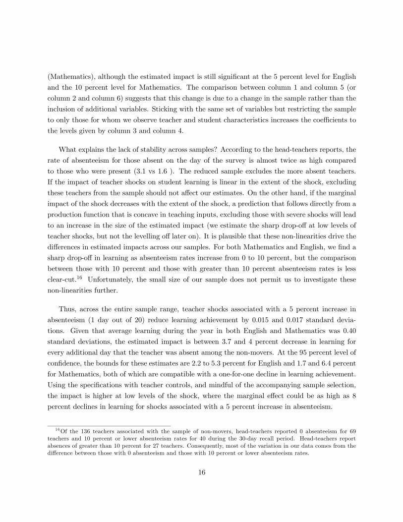
(Mathematics), although the estimated impact is still significant at the 5 percent level for English

and the 10 percent level for Mathematics. The comparison between column 1 and column 5 (or

column 2 and column 6) suggests that this change is due to a change in the sample rather than the

inclusion of additional variables. Sticking with the same set of variables but restricting the sample

to only those for whom we observe teacher and student characteristics increases the coefficients to

the levels given by column 3 and column 4.

What explains the lack of stability across samples? According to the head-teachers reports, the

rate of absenteeism for those absent on the day of the survey is almost twice as high compared

to those who were present (3.1 vs 1.6 ). The reduced sample excludes the more absent teachers.

If the impact of teacher shocks on student learning is linear in the extent of the shock, excluding

these teachers from the sample should not affect our estimates. On the other hand, if the marginal

impact of the shock decreases with the extent of the shock, a prediction that follows directly from a

production function that is concave in teaching inputs, excluding those with severe shocks will lead

to an increase in the size of the estimated impact (we estimate the sharp drop-off at low levels of

teacher shocks, but not the levelling off later on). It is plausible that these non-linearities drive the

differences in estimated impacts across our samples. For both Mathematics and English, we find a

sharp drop-off in learning as absenteeism rates increase from 0 to 10 percent, but the comparison

between those with 10 percent and those with greater than 10 percent absenteeism rates is less

clear-cut.16 Unfortunately, the small size of our sample does not permit us to investigate these

non-linearities further.

Thus, across the entire sample range, teacher shocks associated with a 5 percent increase in

absenteeism (1 day out of 20) reduce learning achievement by 0.015 and 0.017 standard devia-

tions. Given that average learning during the year in both English and Mathematics was 0.40

standard deviations, the estimated impact is between 3.7 and 4 percent decrease in learning for

every additional day that the teacher was absent among the non-movers. At the 95 percent level of

confidence, the bounds for these estimates are 2.2 to 5.3 percent for English and 1.7 and 6.4 percent

for Mathematics, both of which are compatible with a one-for-one decline in learning achievement.

Using the specifications with teacher controls, and mindful of the accompanying sample selection,

the impact is higher at low levels of the shock, where the marginal effect could be as high as 8

percent declines in learning for shocks associated with a 5 percent increase in absenteeism.

16Of the 136 teachers associated with the sample of non-movers, head-teachers reported 0 absenteeism for 69teachers and 10 percent or lower absenteeism rates for 40 during the 30-day recall period. Head-teachers reportabsences of greater than 10 percent for 27 teachers. Consequently, most of the variation in our data comes from thedifference between those with 0 absenteeism and those with 10 percent or lower absenteeism rates.

16

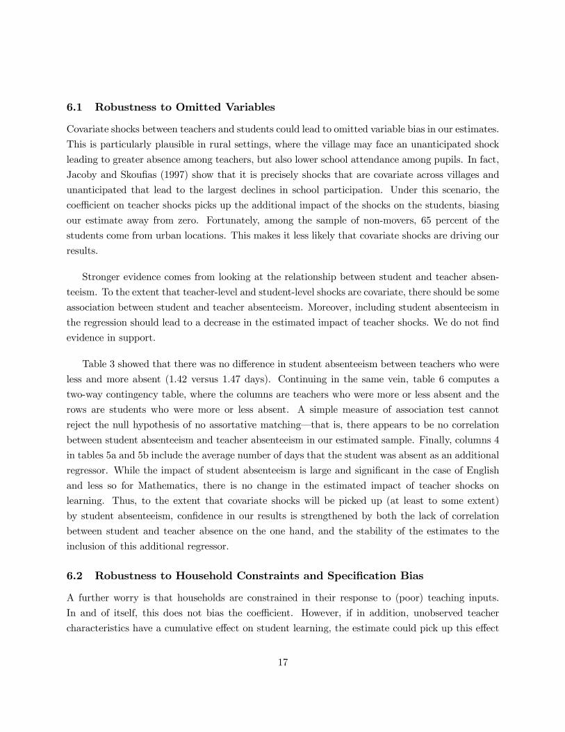
6.1 Robustness to Omitted Variables

Covariate shocks between teachers and students could lead to omitted variable bias in our estimates.

This is particularly plausible in rural settings, where the village may face an unanticipated shock

leading to greater absence among teachers, but also lower school attendance among pupils. In fact,

Jacoby and Skoufias (1997) show that it is precisely shocks that are covariate across villages and

unanticipated that lead to the largest declines in school participation. Under this scenario, the

coefficient on teacher shocks picks up the additional impact of the shocks on the students, biasing

our estimate away from zero. Fortunately, among the sample of non-movers, 65 percent of the

students come from urban locations. This makes it less likely that covariate shocks are driving our

results.

Stronger evidence comes from looking at the relationship between student and teacher absen-

teeism. To the extent that teacher-level and student-level shocks are covariate, there should be some

association between student and teacher absenteeism. Moreover, including student absenteeism in

the regression should lead to a decrease in the estimated impact of teacher shocks. We do not find

evidence in support.

Table 3 showed that there was no difference in student absenteeism between teachers who were

less and more absent (1.42 versus 1.47 days). Continuing in the same vein, table 6 computes a

two-way contingency table, where the columns are teachers who were more or less absent and the

rows are students who were more or less absent. A simple measure of association test cannot

reject the null hypothesis of no assortative matching–that is, there appears to be no correlation

between student absenteeism and teacher absenteeism in our estimated sample. Finally, columns 4

in tables 5a and 5b include the average number of days that the student was absent as an additional

regressor. While the impact of student absenteeism is large and significant in the case of English

and less so for Mathematics, there is no change in the estimated impact of teacher shocks on

learning. Thus, to the extent that covariate shocks will be picked up (at least to some extent)

by student absenteeism, confidence in our results is strengthened by both the lack of correlation

between student and teacher absence on the one hand, and the stability of the estimates to the

inclusion of this additional regressor.

6.2 Robustness to Household Constraints and Specification Bias

A further worry is that households are constrained in their response to (poor) teaching inputs.

In and of itself, this does not bias the coefficient. However, if in addition, unobserved teacher

characteristics have a cumulative effect on student learning, the estimate could pick up this effect

17

as well. Suppose unmotivated teachers are more absent. As long as the lack of motivation affects

only the scores in the first year (that is, it is a one-time negative shock), it does not impact on

the change in scores between the first and the second year. However, if teacher motivation affects

how much students learn in every year, our measure of teacher shocks would pick up both intrinsic

motivation as well as time-varying shocks to teaching inputs. Even with such cumulative effects, the

estimated coefficient is still identified if households are able to respond to teacher motivation–the

impact of lower motivation would be attenuated through greater household participation. We have

less to say about how the combination of cumulative teacher effects and household-level constraints

may bias our coefficients. To estimate such persistent effects requires data from at least 3 points

in time, and this is a hard requirement in low-income countries. Nevertheless, suggestive evidence

along two fronts indicates that these persistent impacts are not critical to our findings.

First, to the extent that teacher effects are cumulative, we should also find that the first-year

test scores are correspondingly low for students associated with more absent teachers. This is not

the case. Table 7 reports results of a regression of baseline test scores on the number of days

absent and teacher characteristics. Columns 1 and 2, and 5 and 6 report coefficients for the full

sample, while the other columns report results for the non-mover sample. For both Mathematics

and English, we fail to find any association between baseline test scores and the head-teacher report

of absenteeism. For both subjects, the point estimates and the significance is very low.

Second, we find no supporting evidence in observables. Returning to tables 5a and 5b, tests for

the joint significance of teacher characteristics report F-statistics in the range of 0.06 (English) and

0.72 (Mathematics), both of which are insignificant at the 50-percent level of confidence. Further,

the inclusion (or not) of teacher characteristics does not alter the estimated impact of teacher

shocks.

7 Movers: A Puzzle and Potential Reconciliations

In the case of the non-movers, the choice of sample “differences-out” the non-time varying un-

observable inputs of the teacher and the estimate accurately captures the effect of time-varying

shocks to teaching inputs on learning. However, our sample of non-movers is different from the

movers (see table 3): since the policy of teachers remaining with the same cohort of students was

implemented in larger schools, the non-movers tend to be concentrated in urban areas and come

from households that are one-third of a standard deviation richer on average. A priori, one may

expect that the effect of teacher shocks is lower in the sample of non-movers compared to movers–

to the extent that wealth and urbanization capture substitution possibilities (more wealthy and

18

more urban households are more likely to hire private tutors), negative shocks should have a larger

impact on movers than non-movers.

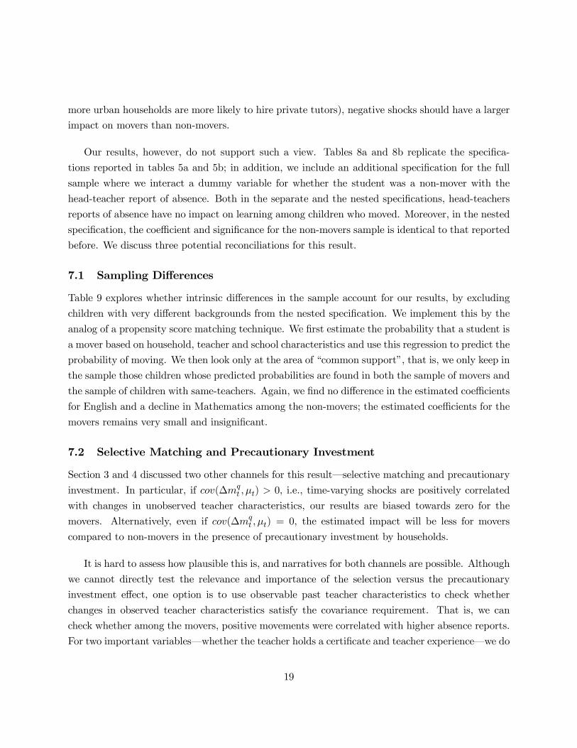
Our results, however, do not support such a view. Tables 8a and 8b replicate the specifica-

tions reported in tables 5a and 5b; in addition, we include an additional specification for the full

sample where we interact a dummy variable for whether the student was a non-mover with the

head-teacher report of absence. Both in the separate and the nested specifications, head-teachers

reports of absence have no impact on learning among children who moved. Moreover, in the nested

specification, the coefficient and significance for the non-movers sample is identical to that reported

before. We discuss three potential reconciliations for this result.

7.1 Sampling Differences

Table 9 explores whether intrinsic differences in the sample account for our results, by excluding

children with very different backgrounds from the nested specification. We implement this by the

analog of a propensity score matching technique. We first estimate the probability that a student is

a mover based on household, teacher and school characteristics and use this regression to predict the

probability of moving. We then look only at the area of “common support”, that is, we only keep in

the sample those children whose predicted probabilities are found in both the sample of movers and

the sample of children with same-teachers. Again, we find no difference in the estimated coefficients

for English and a decline in Mathematics among the non-movers; the estimated coefficients for the

movers remains very small and insignificant.

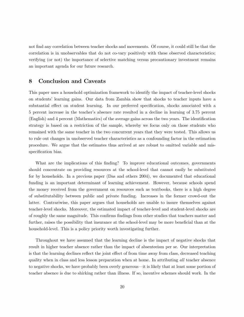
7.2 Selective Matching and Precautionary Investment

Section 3 and 4 discussed two other channels for this result–selective matching and precautionary

investment. In particular, if cov(∆mqt , µt) > 0, i.e., time-varying shocks are positively correlated

with changes in unobserved teacher characteristics, our results are biased towards zero for the

movers. Alternatively, even if cov(∆mqt , µt) = 0, the estimated impact will be less for movers

compared to non-movers in the presence of precautionary investment by households.

It is hard to assess how plausible this is, and narratives for both channels are possible. Although

we cannot directly test the relevance and importance of the selection versus the precautionary

investment effect, one option is to use observable past teacher characteristics to check whether

changes in observed teacher characteristics satisfy the covariance requirement. That is, we can

check whether among the movers, positive movements were correlated with higher absence reports.

For two important variables–whether the teacher holds a certificate and teacher experience–we do

19

not find any correlation between teacher shocks and movements. Of course, it could still be that the

correlation is in unobservables that do not co-vary positively with these observed characteristics;

verifying (or not) the importance of selective matching versus precautionary investment remains

an important agenda for our future research.

8 Conclusion and Caveats

This paper uses a household optimization framework to identify the impact of teacher-level shocks

on students’ learning gains. Our data from Zambia show that shocks to teacher inputs have a

substantial effect on student learning. In our preferred specification, shocks associated with a

5 percent increase in the teacher’s absence rate resulted in a decline in learning of 3.75 percent

(English) and 4 percent (Mathematics) of the average gains across the two years. The identification

strategy is based on a restriction of the sample, whereby we focus only on those students who

remained with the same teacher in the two concurrent years that they were tested. This allows us

to rule out changes in unobserved teacher characteristics as a confounding factor in the estimation

procedure. We argue that the estimates thus arrived at are robust to omitted variable and mis-

specification bias.

What are the implications of this finding? To improve educational outcomes, governments

should concentrate on providing resources at the school-level that cannot easily be substituted

for by households. In a previous paper (Das and others 2004), we documented that educational

funding is an important determinant of learning achievement. However, because schools spend

the money received from the government on resources such as textbooks, there is a high degree

of substitutability between public and private funding. Increases in the former crowd-out the

latter. Contrariwise, this paper argues that households are unable to insure themselves against

teacher-level shocks. Moreover, the estimated impact of teacher-level and student-level shocks are

of roughly the same magnitude. This confirms findings from other studies that teachers matter and

further, raises the possibility that insurance at the school-level may be more beneficial than at the

household-level. This is a policy priority worth investigating further.

Throughout we have assumed that the learning decline is the impact of negative shocks that

result in higher teacher absence rather than the impact of absenteeism per se. Our interpretation

is that the learning declines reflect the joint effect of from time away from class, decreased teaching

quality when in class and less lesson preparation when at home. In attributing all teacher absence

to negative shocks, we have probably been overly generous–it is likely that at least some portion of

teacher absence is due to shirking rather than illness. If so, incentive schemes should work. In the

20

United States, Jacobson’s work (Jacobson 1989 and Jacobson 1991) shows that payment incentives

do lead to declines in absenteeism. However, the welfare impacts are less certain.

Jacobson (1989) documents how a payment incentive scheme led to a decline in teacher absen-

teeism. Nevertheless, one year later a fact-finding mission concludes that:

“While the District’s attendance statistics for the past several school years may lead some to

conclude that attendance improved (...) the fact finder does not believe the record before him estab-

lished that improved attendance rate (...) raised the quality of teachers or teaching in the District.

In fact, the District and Association expressed their agreement that they knew of no way to mea-

sure the effectiveness of a sick teacher who came to work to assure receiving a higher share of EIT

money vs. that of a sick teacher who stayed home to recuperate while a substitute taught his/her

classes (...) I conclude that an attendance based criterion for the 1987/88 EIT distribution simply

would not serve to promote the "excellence in teaching" envisioned by the State Legislature and the

Governor (PERB 1988: 9-10).”

The situation in low-income countries may be very different. Certainly, studies in India (Chaud-

hury and others 2005) suggest that teacher absenteeism is largely due to shirking rather than ill-

ness. Jacobson’s work however, cautions us in extrapolating views from one continent to another.

If teachers in Zambia and other Sub-Saharan countries are absent because they shirk and incen-

tive schemes and greater accountability lead both to greater attendance and better performance,

then such schemes can lead to better learning outcomes. However, if teachers’ utility functions are

altruistic so that most absenteeism is “genuine”, incentive schemes might hurt teacher motivation.

This conflict between treating teachers as “professionals” who respond to monetary incentives and

thinking of them as “dedicated to students’ needs” remains at the center of a contentious debate

in the United States. Although research in low-income countries is at a nascent stage, with absen-

teeism rates approaching 25 percent in some countries, steps towards a deeper understanding are

critical.

Our findings also raise a methodological issue. The results obtained on the cohort of children

who stayed with the same teacher, do not extend to the entire sample. The policy of retaining the

same teacher for the student-cohort was implemented only for larger schools, so non-movers come

from more urban schools where the teachers are better (more experienced and better trained),

families are richer and parents are more educated. With better access to markets for private

tuition and home schooling, we expected the impact of teacher shocks to be lower among the

sample of children who are non-movers. Intriguingly we found no impact of teacher shocks on

student learning among the movers in our sample. We suggested two reasons for this finding. If the

21

sample of children who switched teachers were not randomly assigned, selective matching might

bias our estimate. A second interesting possibility was the role of uncertainty in teaching inputs on

household investments. The model shows that greater uncertainty in teaching inputs leads to an

ex ante response among households through greater precautionary spending. Faced with greater

uncertainty in teaching inputs, the movers would have higher precautionary spending and thus be

less susceptible to ex post shocks.

We would have liked to directly test which of these mechanisms is responsible for the difference

in estimates. Do households really undertake precautionary schooling investments? That is, do

parents of movers spend more time or money with their children than those of non-movers? Un-

fortunately, our data on household inputs does not allow us to investigate this directly. Although

we surveyed households matched to these schools (see Das and others 2004a), these were all rural

households and our sample of non-movers is too small to draw any meaningful inferences.

If we believe that households play an important role in determining educational outcomes

of their children, this paper suggests a direction for future work. Using a model allowing for

household responses to teacher and school inputs allows for richer insights than standard production

function approaches. The impact of current year shocks on learning achievement depends on other

sources of uncertainty (non time-varying attributes of the teacher in this paper) and this has

important implications for future evaluation work.17 Currently there is little research on the link

between household and school inputs, and none on the precautionary motive discussed in this paper.

Evidence either way would be helpful.

17Suppose that an experiment were designed to study the effect of absenteeism on learning achievement. The”treatment on the treated” estimator will represent the average effect, averaged across children who changed andremained with the same teacher. This paper suggests that the external validity of the experiment may be compromiseddue to this important source of heterogeneity–an empirical implication is to try and capture information on this andother changes that have occurred during the year of the experiment.

22

The word processed describes informally produced works that may not be commonly available

through library systems.

References

[1] Angrist, Joshua and Victor Lavy. 2001. “Does Teacher Training Affect Learning? Evidence

from Matched Comparisons in Jerusalem Public Schools.” Journal of Labor Economics, 343-

369.

[2] Bell, Clive, Shanta Devarajan and Gersbach, H. 2003. “The Long Run Economic Costs of

AIDS. Theory and an Application to South Africa.” Policy Research Working Paper 3518,

World Bank, Washington, D.C.

[3] Bennell, Paul, 2005. “The Impact of the AIDS Epidemic on Teachers in Sub Saharan Africa”

Journal of Development Studies, 41 (3): 440-466.

[4] Chaudhury, Nazmul., Jeffrey Hammer, Michale Kremer,K. Muralidharan and Halsey Rogers.

2004. ”Teacher and Health Care Provider Absenteeism: A Multi-Country Study.” World Bank:

Washington, DC. Processed.

[5] Chaudhury, Nazmul and Jeffrey Hammer. “Ghost Doctors: Absenteeism in Bangladeshi Health

Facilities.” World Bank Economic Review, 18(3): 423-41.

[6] Das, Jishnu, Stefan Dercon, James Habyarimana, and Pramila Krishnan. 2004a. "When Can

School Inputs Improve Test Scores” Policy Research Working Paper 3217, World Bank, Wash-

ington, D.C.

[7] Das, Jishnu, Stefan Dercon, James Habyarimana, and Pramila Krishnan. 2004b. "Public and

Private Funding in Zambian Basic Education: Rules Vs. Discretion". Africa Human Develop-

ment Working Paper Series #62. Washington D.C.: The World Bank.

[8] de Janvry, Alain, Frederico Finan, Elisabeth Sadoulet, and Renos Vakis. November 2004. “Can

Conditionnal Cash Transfers Serve as Safety Nets to Keep Children at School and out of the

Labor Market?” University of California. Berkeley. Processed.

[9] Deaton, Angus. 1992. Understanding Consumption. Oxford: Clarendon Press.

[10] Deaton, Angus, and John Muellbauer. 1980. “Economics and Consumer Behavior.” Cam-

bridge. UK: Cambridge University Press.

23

[11] Ehrenberg, Robert. G, Ehrenberg R. A, Rees, D and Ehrenberg E, 1991. “School District Leave

Policies, Teacher Absenteeism, and Student Achievement” Journal of Human Resources, 26(1):

72-105

[12] Foster, Andrew. 1995. “Prices, Credit Markets and Child Growth in Low-Income Rural Areas”

The Economic Journal 105 (430): 551-570.

[13] Glewwe, Paul, Michael Kremer and Sylvie Moulin. 2001. “Textbooks and Test scores: Evidence

from a Prospective Evaluation in Kenya”, University of Minnesota. Processed.

[14] Grassly, Nicholas C., Kamal Desai, Elisabetta Pegurri, Alfred Sikazwe, Irene Malambo,

Clement Siamatowe, and Don Bundy. 2003. “The economic impact of HIV/AIDS on the edu-

cation sector in Zambia.” AIDS 17(7):1039-1044.

[15] Hanushek, Eric. 1986. “The Economics of Schooling: Production and Efficiency in Public

Schools”, Journal of Economic Literature XXIV, 1141-1177.

[16] Hanushek, E., Kain, J. and Rivkin, S., 1998 “Teachers, schools and academic achievement”

NBER Working Paper, Number w6691.

[17] Jacoby, Hanan G., and Emmanuel Skoufias. 1997. “Risk, Financial Markets, and Human Cap-

ital in a Developing Country.” Review of Economic Studies 64(3): 311-335.

[18] Jacobson, Stephen. 1989. “The Effects of Pay Incentives on Teacher Absenteeism.” Journal of

Human Resources 243(2): 280-286.

[19] Jacobson, Stephen. 1991. “Attendance Incentives and Teacher Absenteeism.” Planning and

Changing 21(2): 78-93.

[20] Park, Albert and Hannum E, 2002. “Do Teachers Affect Learning in Developing Countries?:

Evidence from Student-Teacher data from China”, Harvard University. Processed.

[21] Rockoff, Jonah E. 2004. “The Impact of Teachers on Student Achievement: Evidence from

Panel Data”, American Economic Review, 94(2): 247-252.

[22] Sandmo, A., 1969, "Capital risk, Consumption and Portfolio Choice", Econometrica, 37: 586-

599.

[23] Todd, Petra and Kenneth Wolpin. 2003. “On the Specification and Estimation of the Produc-

tion Function for Cognitive Achievement”, The Economic Journal 113 (February): F3-33.

[24] World Bank.2003. World Development Report 2004: Making Services Work for the Poor.

Washington, D.C.: The World Bank.

24

9 Appendix 1: Measuring Teacher Absence

We collected a spot measure of teacher absence by checking attendance on the day of the survey

for all teachers in small schools and a non-random sample of 20 teachers in larger schools. Since

this is a prevalence rate, a spot absence rate of 20 percent does not distinguish between all teachers

being absent 20 percent of the time, or half the teachers being absent 40 percent of the time. If half

of the teachers have an absenteeism incidence of 40 percent and the other half are always present,

to distinguish between the two types of teachers with 95 percent confidence, we would require at

least 6 visits (assuming that absence follows a Bernouli process). We also collected a self-reported

absence profile over the last 30 days for teachers matched to pupils. This measure is biased because

it is missing for teachers absent on the day. Also, it is plausible that low-quality teachers may

report absenteeism in different ways than high-quality teachers.

The differences between the measures appear to be in line with expectations regarding the bias

and noise entailed in self-reported or spot absenteeism measures. The extent of these differences

can be partially assessed by using the sampling differences between the different measures of absen-

teeism. For instance we can check for a selection effect in the self-reported measure (we don’t have

a report for those who were absent on the day) by comparing the reports of the head-teacher for the

sample who were present on the day of the survey and those who were not. Using the head-teacher’s

report, teachers who were absent on the day of the survey miss an average of 2.39 days compared

to 1.5 days for teachers who were present. This difference is significant at the 5-percent level, also

suggesting problems with the spot measure based on those absent at the time of the visit.

We also find evidence of reporting bias in the self-reported measure. To investigate the reporting

biases of the self-report, we divide teachers into those who had pupils with high and low learning

gains, and examine the correlation between the self-report and the head-teacher report for these

two groups. If there are self-reporting biases, the correlation between the two reports should be

higher for the teachers with high-performing children compared to teachers with low-learning gains.

The correlation between self-reported and head-teacher for the “good” teachers is 0.39 compared to

0.28 for the “bad” teachers. Gains in English suggest a similar, albeit weaker result. This pattern

is broadly consistent with “bad” teachers under-reporting duration of absence assuming that the

head-teacher’s report is the true measure.

10 Appendix 2: Ex Ante Risk and Household Investment

To develop the circumstances under which greater ex ante risk leads to larger household investment,

we introduce risk in a specific way. Let mt = mqt + a + µt, whereby a = a > 0 if the teacher is

25

of high quality, and a = −a if the teacher is of low quality. Increases in a would then imply anincrease in risk in the sense of a standard increase in mean-preserving spread. A sufficient condition

for household spending on education to increase in risk is that∂U∂TStπt

is decreasing and convex in

mt. We continue to impose (as in Das and others (2004a)) the following assumptions:

[A1] Household utility is additively separable and of the CRRA form.

[A2] TSt = (1− δ)TSt−1 + F (wt, zt, µ, η) where the Hessian of F (.) is negative semi-definite.Under [A1] marginal utility is defined as TS−ρt , with ρ the coefficient of relative risk aversion.

Using [A2] and the implicit function theorem with (5), we have

dπtdmt

= −Fztmt

F 2zt0 if Fztmt 0 (11)

The sign of the cross partial depends on whether the household can respond to changes to teacher

inputs. If Fztmt = 0, households are unable to respond to changes in teacher inputs. This might be a

consequence of credit constraints, inability of parents to substitute either via a lack of ability/time

and the absence of markets for private tuition. If, however, households are able to respond to

changes in teacher inputs and household and teacher inputs are technical substitutes (Fztmt < 0),

increases in teacher inputs at t will increase the relative user-cost of boosting cognitive achievement

at t. The reverse is true if teacher and household inputs are technical complements (Fztmt > 0).

It follows directly that∂U∂TStπt

will be decreasing in mt if teacher and household inputs are technical

substitutes and if households are risk averse:

d∂U∂TStπt

dmt=− ∂πt

∂mt. ∂U∂TSt

+ ∂2U∂TS2t

.Fmt .πt

π2t< 0 (12)

In (12), the first term in the numerator is negative if inputs are technical substitutes and the

second term is negative if households are risk averse. Furthermore, it can be shown that a sufficient

condition for∂U∂TStπt

to be convex in teacher inputs is that inputs are technical substitutes, households

are risk averse, the marginal utility of additional cognitive achievement is convex, and the user-cost

is concave in m (it increases at a decreasing rate). Convex marginal utility is satisfied under CRRA

.The user-cost is concave in m if FzFmmz ≥ 2(Fzm)218.

18Concavity of the user-cost is not a necessary condition: even with convexity of user-cost, sufficiently high risk

aversion or substantial convexity of marginal utility could result in the convexity of∂U∂TStπt

.

26

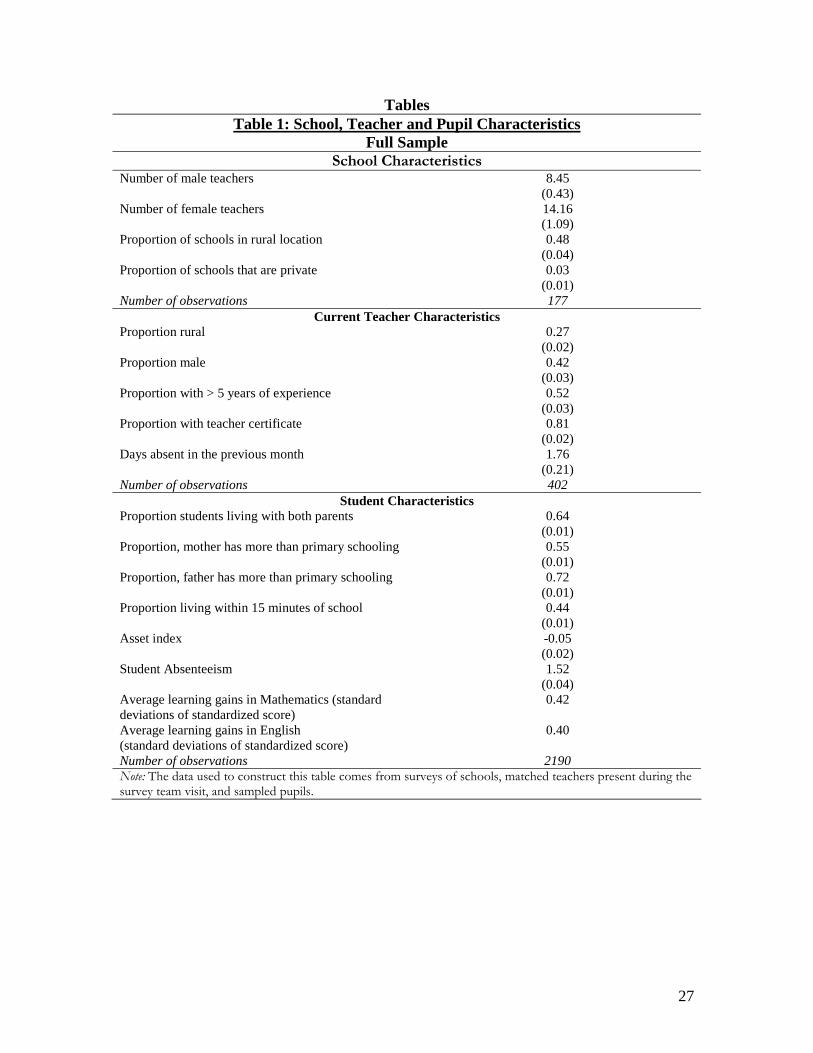
27

Tables Table 1: School, Teacher and Pupil Characteristics

Full Sample School Characteristics

Number of male teachers 8.45 (0.43)

Number of female teachers 14.16 (1.09)

Proportion of schools in rural location 0.48 (0.04)

Proportion of schools that are private 0.03 (0.01)

Number of observations 177 Current Teacher Characteristics

Proportion rural 0.27 (0.02)

Proportion male 0.42 (0.03)

Proportion with > 5 years of experience 0.52 (0.03)

Proportion with teacher certificate 0.81 (0.02)

Days absent in the previous month 1.76 (0.21)

Number of observations 402 Student Characteristics

Proportion students living with both parents 0.64 (0.01)

Proportion, mother has more than primary schooling 0.55 (0.01)

Proportion, father has more than primary schooling 0.72 (0.01)

Proportion living within 15 minutes of school 0.44 (0.01)

Asset index -0.05 (0.02)

Student Absenteeism 1.52 (0.04)

Average learning gains in Mathematics (standard deviations of standardized score)

0.42

Average learning gains in English (standard deviations of standardized score)

0.40

Number of observations 2190 Note: The data used to construct this table comes from surveys of schools, matched teachers present during the survey team visit, and sampled pupils.

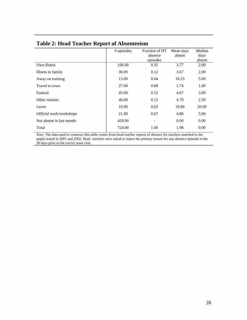
28

Table 2: Head Teacher Report of Absenteeism # episodes Fraction of HT

absence episodes

Mean days absent

Median days

absent Own illness 106.00 0.35 3.77 2.00

Illness in family 36.00 0.12 3.67 2.00

Away on training 13.00 0.04 10.23 5.00

Travel to town 27.00 0.09 1.74 1.00

Funeral 45.00 0.15 4.67 3.00

Other reasons 46.00 0.15 4.70 2.50

Leave 10.00 0.03 19.00 20.00

Official work/workshops 21.00 0.07 4.86 5.00

Not absent in last month 420.00 - 0.00 0.00

Total 724.00 1.00 1.98 0.00

Note: The data used to construct this table comes from head teacher reports of absence for teachers matched to the pupils tested in 2001 and 2002. Head teachers were asked to report the primary reason for any absence episode in the 30 days prior to the survey team visit.

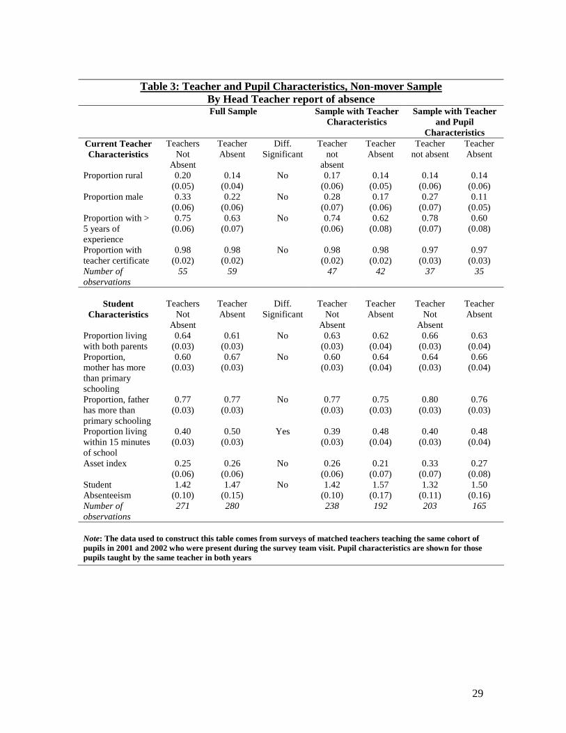
29

Table 3: Teacher and Pupil Characteristics, Non-mover Sample

By Head Teacher report of absence Full Sample Sample with Teacher

Characteristics Sample with Teacher

and Pupil Characteristics

Current Teacher Characteristics

Teachers Not

Absent

Teacher Absent

Diff. Significant

Teacher not

absent

Teacher Absent

Teacher not absent

Teacher Absent

Proportion rural 0.20 (0.05)

0.14 (0.04)

No 0.17 (0.06)

0.14 (0.05)

0.14 (0.06)

0.14 (0.06)

Proportion male 0.33 (0.06)

0.22 (0.06)

No 0.28 (0.07)

0.17 (0.06)

0.27 (0.07)

0.11 (0.05)

Proportion with > 5 years of experience

0.75 (0.06)

0.63 (0.07)

No 0.74 (0.06)

0.62 (0.08)

0.78 (0.07)

0.60 (0.08)

Proportion with teacher certificate

0.98 (0.02)

0.98 (0.02)

No 0.98 (0.02)

0.98 (0.02)

0.97 (0.03)

0.97 (0.03)

Number of observations

55 59 47 42 37 35

Student

Characteristics Teachers

Not Absent

Teacher Absent

Diff. Significant

Teacher Not

Absent

Teacher Absent

Teacher Not

Absent

Teacher Absent

Proportion living with both parents

0.64 (0.03)

0.61 (0.03)

No 0.63 (0.03)

0.62 (0.04)

0.66 (0.03)

0.63 (0.04)

Proportion, mother has more than primary schooling

0.60 (0.03)

0.67 (0.03)

No 0.60 (0.03)

0.64 (0.04)

0.64 (0.03)

0.66 (0.04)

Proportion, father has more than primary schooling

0.77 (0.03)

0.77 (0.03)

No 0.77 (0.03)

0.75 (0.03)

0.80 (0.03)

0.76 (0.03)

Proportion living within 15 minutes of school

0.40 (0.03)

0.50 (0.03)

Yes 0.39 (0.03)

0.48 (0.04)

0.40 (0.03)

0.48 (0.04)

Asset index 0.25 (0.06)

0.26 (0.06)

No 0.26 (0.06)

0.21 (0.07)

0.33 (0.07)

0.27 (0.08)

Student Absenteeism

1.42 (0.10)

1.47 (0.15)

No 1.42 (0.10)

1.57 (0.17)

1.32 (0.11)

1.50 (0.16)

Number of observations

271 280 238 192 203 165

Note: The data used to construct this table comes from surveys of matched teachers teaching the same cohort of pupils in 2001 and 2002 who were present during the survey team visit. Pupil characteristics are shown for those pupils taught by the same teacher in both years

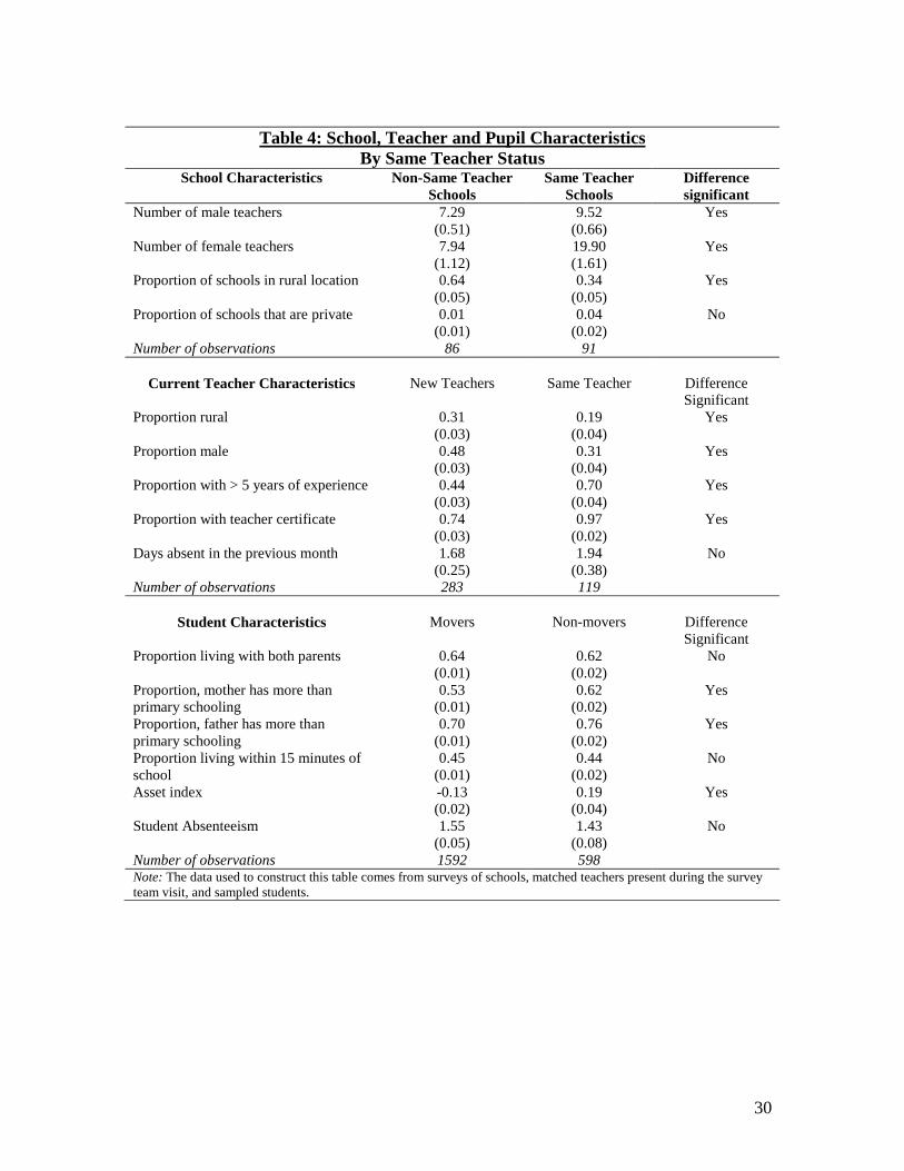
30

Table 4: School, Teacher and Pupil Characteristics

By Same Teacher Status School Characteristics Non-Same Teacher

Schools Same Teacher

Schools Difference significant

Number of male teachers 7.29 (0.51)

9.52 (0.66)

Yes

Number of female teachers 7.94 (1.12)

19.90 (1.61)

Yes

Proportion of schools in rural location 0.64 (0.05)

0.34 (0.05)

Yes

Proportion of schools that are private 0.01 (0.01)

0.04 (0.02)

No

Number of observations 86 91

Current Teacher Characteristics New Teachers Same Teacher Difference Significant

Proportion rural 0.31 (0.03)

0.19 (0.04)

Yes

Proportion male 0.48 (0.03)

0.31 (0.04)

Yes

Proportion with > 5 years of experience 0.44 (0.03)

0.70 (0.04)

Yes

Proportion with teacher certificate 0.74 (0.03)

0.97 (0.02)

Yes

Days absent in the previous month 1.68 (0.25)

1.94 (0.38)

No

Number of observations 283 119

Student Characteristics Movers Non-movers Difference Significant

Proportion living with both parents 0.64 (0.01)

0.62 (0.02)

No

Proportion, mother has more than primary schooling

0.53 (0.01)

0.62 (0.02)

Yes

Proportion, father has more than primary schooling

0.70 (0.01)

0.76 (0.02)

Yes

Proportion living within 15 minutes of school

0.45 (0.01)

0.44 (0.02)

No

Asset index -0.13 (0.02)

0.19 (0.04)

Yes

Student Absenteeism 1.55 (0.05)

1.43 (0.08)

No

Number of observations 1592 598 Note: The data used to construct this table comes from surveys of schools, matched teachers present during the survey team visit, and sampled students.

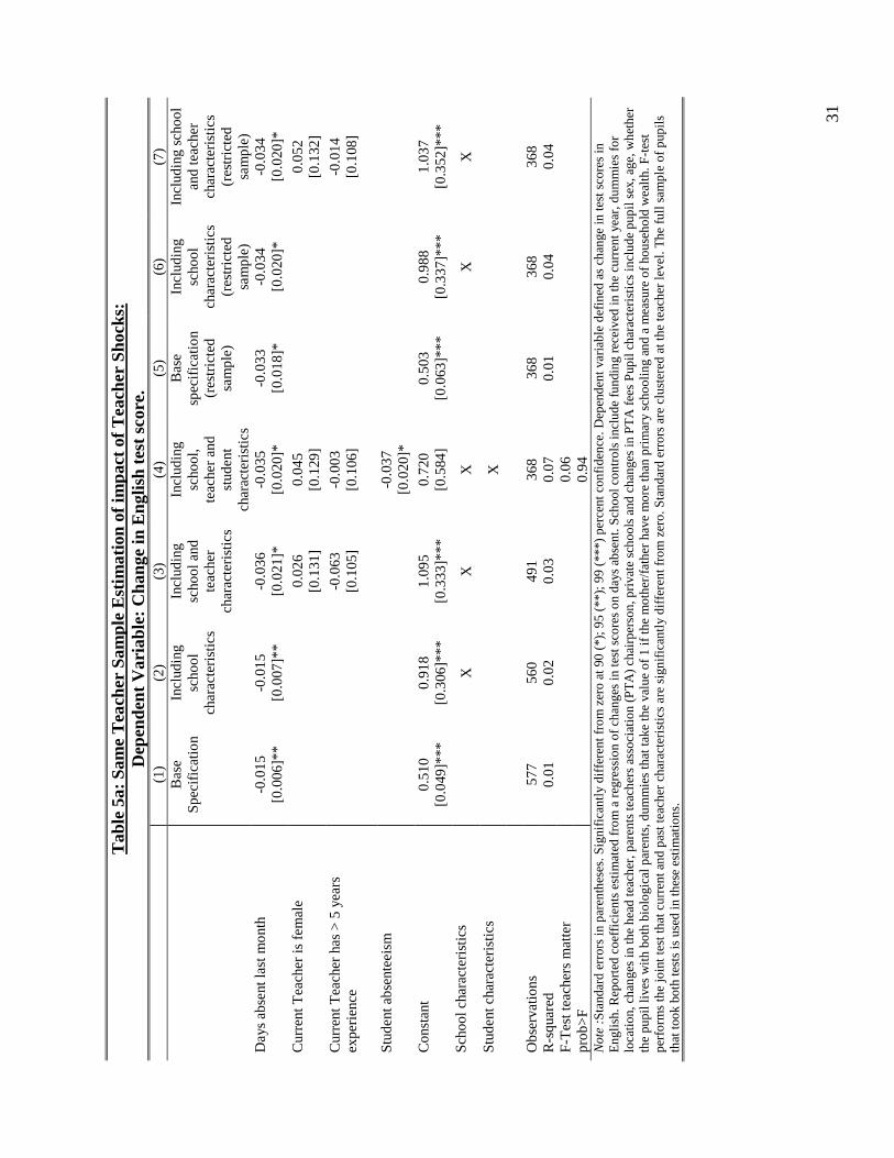
31

Tab

le 5

a: S

ame

Tea

cher

Sam

ple

Est

imat

ion

of im

pact

of

Tea

cher

Sho

cks:

D

epen

dent

Var

iabl

e: C

hang

e in

Eng

lish

test

sco

re.

(1

) (2

) (3

) (4

) (5

) (6

) (7

)

Bas

e Sp

ecif

icat

ion

Incl

udin

g sc

hool

ch

arac

teri

stic

s

Incl

udin

g sc

hool

and

te

ache

r ch

arac

teri

stic

s

Incl

udin

g sc

hool

, te

ache

r an

d st

uden

t ch

arac

teri

stic

s

Bas

e sp

ecif

icat

ion

(res

tric

ted

sam

ple)

Incl

udin

g sc

hool

ch

arac

teri

stic

s (r

estr

icte

d sa

mpl

e)

Incl

udin

g sc

hool

an

d te

ache

r ch

arac

teri

stic

s (r

estr

icte

d sa

mpl

e)

Day

s ab

sent

last

mon

th

-0.0

15

[0.0

06]*

* -0

.015

[0

.007

]**

-0.0

36

[0.0

21]*

-0

.035

[0

.020

]*

-0.0

33

[0.0

18]*

-0

.034

[0

.020

]*

-0.0

34

[0.0

20]*

Cur

rent

Tea

cher

is f

emal

e

0.

026

[0.1

31]

0.04

5 [0

.129

]

0.

052

[0.1

32]

Cur

rent

Tea

cher

has

> 5

yea

rs

expe

rien

ce

-0.0

63

[0.1

05]

-0.0

03

[0.1

06]

-0.0

14

[0.1

08]

Stud

ent a

bsen

teei

sm

-0

.037

[0

.020

]*

Con

stan

t 0.

510

[0.0

49]*

**

0.91

8 [0

.306

]***

1.

095

[0.3

33]*

**

0.72

0 [0

.584

] 0.

503

[0.0

63]*

**

0.98

8 [0

.337

]***

1.

037

[0.3

52]*

**

Scho

ol c

hara

cter

isti

cs

X

X

X

X

X

Stud

ent c

hara

cter

istic

s

X

Obs

erva

tions

57

7 56

0 49

1 36

8 36

8 36

8 36

8 R

-squ

ared

0.

01

0.02

0.

03

0.07

0.

01

0.04

0.

04

F-T

est t

each

ers

mat

ter

0.

06

pr

ob>

F

0.94

Not

e :S

tand

ard

erro

rs in

par

enth

eses

. Sig

nifi

cant

ly d

iffe

rent

fro

m z

ero

at 9

0 (*

); 9

5 (*

*); 9

9 (*

**)

perc

ent c

onfi

denc

e. D

epen

dent

var

iabl

e de

fine

d as

cha

nge

in te

st s

core

s in

E

ngli

sh. R

epor

ted

coef

fici

ents

est

imat

ed f

rom

a r

egre

ssio

n of

cha

nges

in te

st s

core

s on

day

s ab

sent

. Sch

ool c

ontr

ols

incl

ude

fund

ing

rece

ived

in th

e cu

rren

t yea

r, d

umm

ies

for

loca

tion

, cha

nges

in th

e he

ad te

ache

r, p

aren

ts te

ache

rs a

ssoc

iati

on (

PT

A)

chai

rper

son,

pri

vate

sch

ools

and

cha

nges

in P

TA

fee

s P

upil

cha

ract

eris

tics

incl

ude

pupi

l sex

, age

, whe

ther

th

e pu

pil l

ives

wit

h bo

th b

iolo

gica

l par

ents

, dum

mie

s th

at ta

ke th

e va

lue

of 1

if th

e m

othe

r/fa

ther

hav

e m

ore

than

pri

mar

y sc

hool

ing

and

a m

easu

re o

f ho

useh

old

wea

lth.

F-t

est

perf

orm

s th

e jo

int t

est t

hat c

urre

nt a

nd p

ast t

each

er c

hara

cter

isti

cs a

re s

igni

fica

ntly

dif

fere

nt f

rom

zer

o. S

tand

ard

erro

rs a

re c

lust

ered

at t

he te

ache

r le

vel.

The

ful

l sam

ple

of p

upil

s th

at to

ok b

oth

test

s is

use

d in

thes

e es

tim

atio

ns.

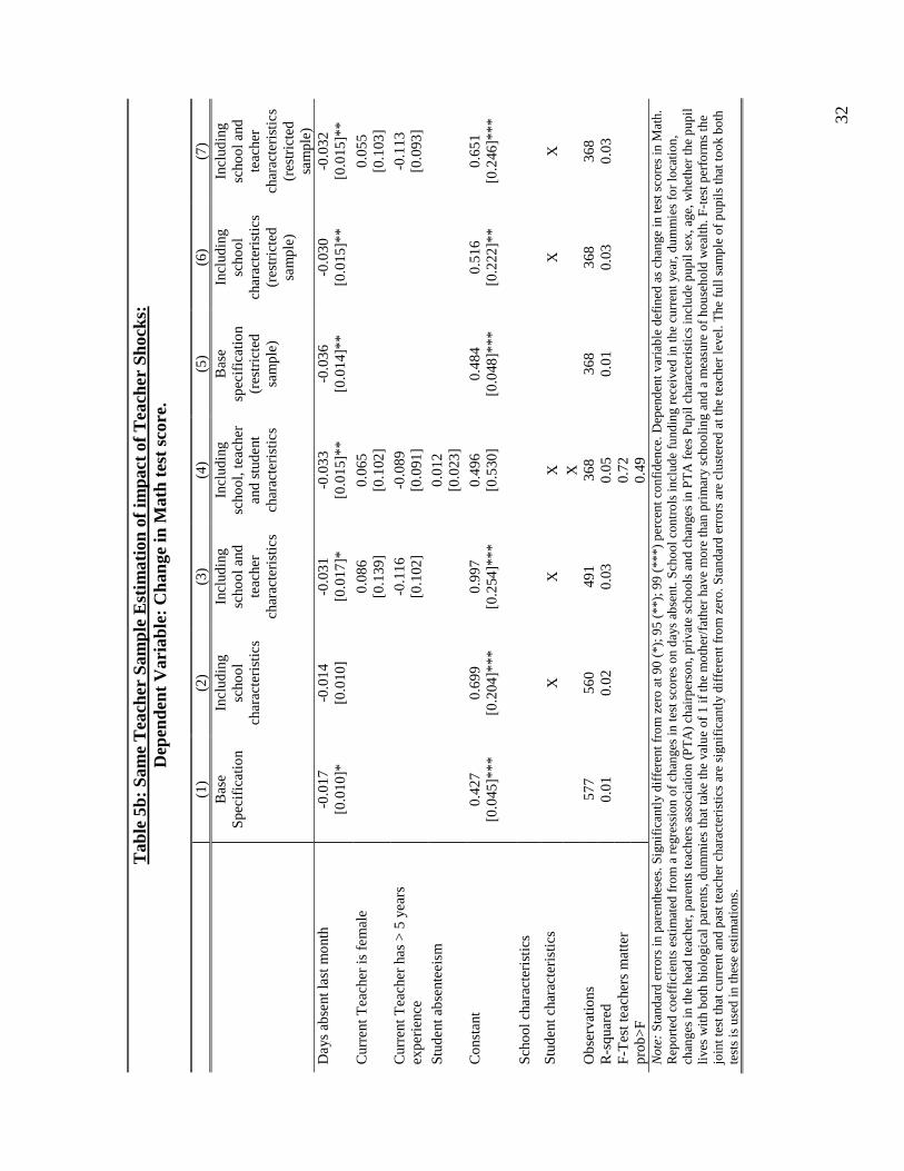
32

T

able

5b:

Sam

e T

each

er S

ampl

e E

stim

atio

n of

impa

ct o

f T

each

er S

hock

s:

Dep

ende

nt V

aria

ble:

Cha

nge

in M

ath

test

sco

re.

(1)

(2)

(3)

(4)

(5)

(6)

(7)

B

ase

Spec

ific

atio

n In

clud

ing

scho

ol

char

acte

rist

ics

Incl

udin

g sc

hool

and

te

ache

r ch

arac

teri

stic

s

Incl

udin

g sc

hool

, tea

cher

an

d st

uden

t ch

arac

teri

stic

s

Bas

e sp

ecif

icat

ion

(res

tric

ted

sam

ple)

Incl

udin

g sc

hool

ch

arac

teri

stic

s (r

estr

icte

d sa

mpl

e)

Incl

udin

g sc

hool

and

te

ache

r ch

arac

teri

stic

s (r

estr

icte

d sa

mpl

e)

Day

s ab

sent

last

mon

th

-0.0

17

[0.0

10]*

-0

.014

[0

.010

] -0

.031

[0

.017

]*

-0.0

33

[0.0

15]*

* -0

.036

[0

.014

]**

-0.0

30

[0.0

15]*

* -0

.032

[0

.015

]**

Cur

rent

Tea

cher

is f

emal

e

0.

086

[0.1

39]

0.06

5 [0

.102

]

0.

055

[0.1

03]

Cur

rent

Tea

cher

has

> 5

yea

rs

expe

rien

ce

-0.1

16

[0.1

02]

-0.0

89

[0.0

91]

-0.1

13

[0.0

93]

Stud

ent a

bsen

teei

sm

0.

012

[0.0

23]

Con

stan

t 0.

427

[0.0

45]*

**

0.69

9 [0

.204

]***

0.

997

[0.2

54]*

**

0.49

6 [0

.530

] 0.

484

[0.0

48]*

**

0.51

6 [0

.222

]**

0.65

1 [0

.246

]***

Scho

ol c

hara

cter

isti

cs

Stud

ent c

hara

cter

istic

s

X

X

X

X

X

X

Obs

erva

tions

57

7 56

0 49

1 36

8 36

8 36

8 36

8 R

-squ

ared

0.

01

0.02

0.

03

0.05

0.

01

0.03

0.

03

F-T

est t

each

ers

mat

ter

0.

72

pr

ob>

F

0.49

Not

e: S

tand

ard

erro

rs in

par

enth

eses

. Sig

nifi

cant

ly d

iffe

rent

fro

m z

ero

at 9

0 (*

); 9

5 (*

*); 9

9 (*

**)

perc

ent c

onfi

denc

e. D

epen

dent

var

iabl

e de

fine

d as

cha

nge

in te

st s

core

s in

Mat

h.

Rep

orte

d co

effi

cien

ts e

stim

ated

fro

m a

reg

ress

ion

of c

hang

es in

test

sco

res

on d

ays

abse

nt. S

choo

l con

trol

s in

clud

e fu

ndin

g re

ceiv

ed in

the

curr

ent y

ear,

dum

mie

s fo

r lo

cati

on,

chan

ges

in th

e he

ad te

ache

r, p

aren

ts te

ache

rs a

ssoc

iati

on (

PT

A)

chai

rper

son,

pri

vate

sch

ools

and

cha

nges

in P

TA

fee

s P

upil

char

acte

rist

ics

incl

ude

pupi

l sex

, age

, whe

ther

the

pupi

l li

ves

wit

h bo

th b

iolo

gica

l par

ents

, dum

mie

s th

at ta

ke th

e va

lue

of 1

if th

e m

othe

r/fa

ther

hav

e m

ore

than

pri

mar

y sc

hool

ing

and

a m

easu

re o

f ho

useh

old

wea

lth.

F-t

est p

erfo

rms

the

join

t tes

t tha

t cur

rent

and

pas

t tea

cher

cha

ract

eris

tics

are

sig

nifi

cant

ly d

iffe

rent

fro

m z

ero.

Sta

ndar

d er

rors

are

clu

ster

ed a

t the

teac

her

leve

l. T

he f

ull s

ampl

e of

pup

ils

that

took

bot

h te

sts

is u

sed

in th

ese

esti

mat

ions

.

33

Tab

le 6

: T

wo-

Way

Ass

ocia

tion

bet

wee

n T

each

er a

nd P

upil

Abs

ente

eism

Les

s ab

sent

teac

hers

M

ore

abse

nt te

ache

rs

L

ess

abse

nt s

tude

nts

312

212

Pre

dict

ed f

requ

ency

31

0 21

3

0.07

8 -0

.094

Mor

e ab

sent

stu

dent

s 85

7 59

1 P

redi

cted

fre

quen

cy

858

589

-0

.047

0.

057

Tes

t sta

tistic

s:

Pea

rson

chi

2(1)

=0.

0203

(P

r =

0.88

7)

Lik

elih

ood-

ratio

chi

2(1)

=0.

0203

(P

r =

0.8

87)

Not

e: T

he ta

ble

abov

e sh

ows

actu

al a

nd p

redi

cted

fre

quen

cies

und

er th

e nu

ll h

ypot

hesi

s th

at th

e co

lum

ns a

nd r

ows

in th

e ta

ble

are

inde

pend

ent.

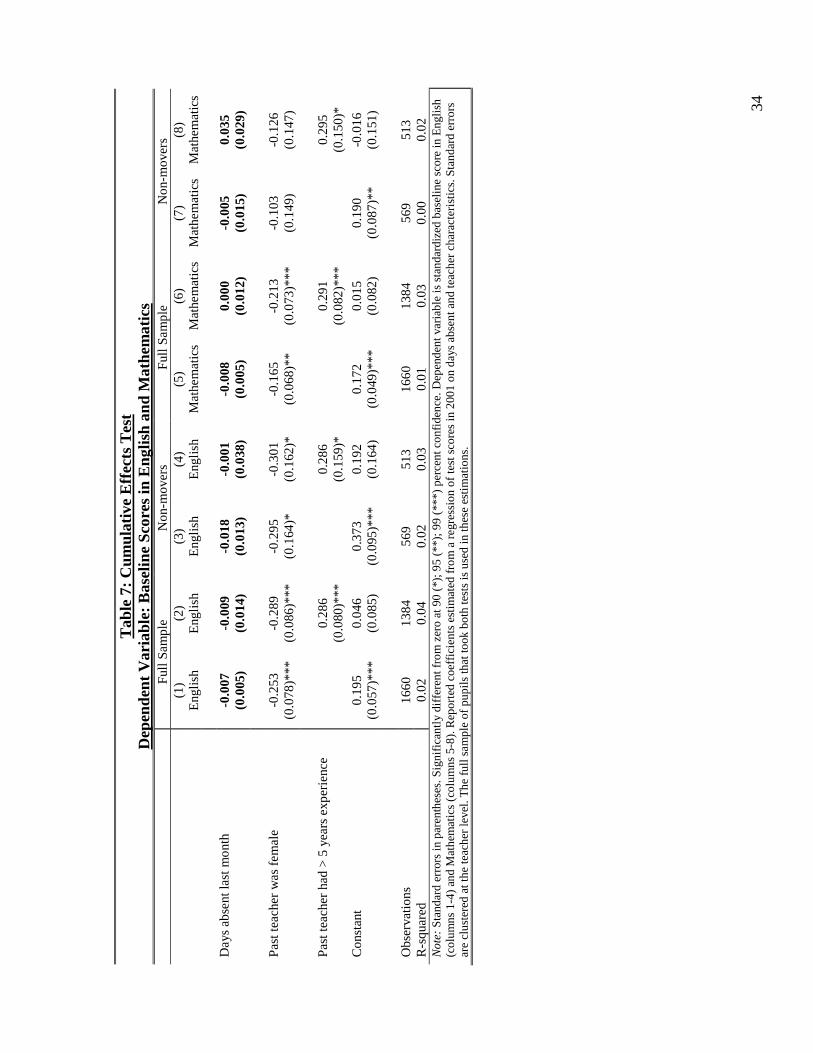
34

T

able

7:

Cum

ulat

ive

Eff

ects

Tes

t D

epen

dent

Var

iabl

e: B

asel

ine

Scor

es in

Eng

lish

and

Mat

hem

atic

s

Full

Sam

ple

Non

-mov

ers

Full

Sam

ple

Non

-mov

ers

(1

) (2

) (3

) (4

) (5

) (6

) (7

) (8

)

Eng

lish

E

ngli

sh

Eng

lish

E

ngli

sh

Mat

hem

atic

s M

athe

mat

ics

Mat

hem

atic

s M

athe

mat

ics

D

ays

abse

nt la

st m

onth

-0

.007

(0

.005

) -0

.009

(0

.014

) -0

.018

(0

.013

) -0

.001

(0

.038

) -0

.008

(0

.005

) 0.

000

(0.0

12)

-0.0

05

(0.0

15)

0.03

5 (0

.029

)

Pas

t tea

cher

was

fem

ale

-0.2

53

(0.0

78)*

**

-0.2

89

(0.0

86)*

**

-0.2

95

(0.1

64)*

-0

.301

(0

.162

)*

-0.1

65

(0.0

68)*

* -0

.213

(0

.073

)***

-0

.103

(0

.149

) -0

.126

(0

.147

)

P

ast t

each

er h

ad >

5 y

ears

exp

erie

nce

0.

286

(0.0

80)*

**

0.

286

(0.1

59)*

0.29

1 (0

.082

)***

0.29

5 (0

.150

)*

Con

stan

t 0.

195

(0.0

57)*

**

0.04

6 (0

.085

) 0.

373

(0.0

95)*

**

0.19

2 (0

.164

) 0.

172

(0.0

49)*

**

0.01

5 (0

.082

) 0.

190

(0.0

87)*

* -0

.016

(0

.151

)

O

bser

vatio

ns

1660

13

84

569

513

1660

13

84

569

513

R-s

quar

ed

0.02

0.

04

0.02

0.

03

0.01

0.

03

0.00

0.

02

Not

e: S

tand

ard

erro

rs in

par

enth

eses

. Sig

nifi

cant

ly d

iffe

rent

fro

m z

ero

at 9

0 (*

); 9

5 (*

*); 9

9 (*

**)

perc

ent c

onfi

denc

e. D

epen

dent

var

iabl

e is

sta

ndar

dize

d ba

seli

ne s

core

in E

ngli

sh

(col

umns

1-4

) an

d M

athe

mat

ics

(col

umns

5-8

). R

epor

ted

coef

fici

ents

est

imat

ed f

rom

a r

egre

ssio

n of

test

sco

res

in 2

001

on d

ays

abse

nt a

nd te

ache

r ch

arac

teri

stic

s. S

tand

ard

erro

rs

are

clus

tere

d at

the

teac

her

leve

l. T

he f

ull s

ampl

e of

pup

ils

that

took

bot

h te

sts

is u

sed

in th

ese

esti

mat

ions

.

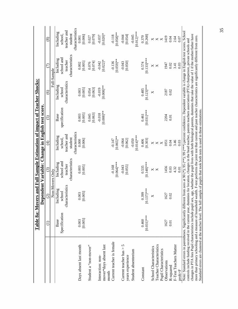
35

T

able

8a:

Mov

ers

and

Ful

l Sam

ple

Est

imat

ion

of im

pact

of

Tea

cher

Sho

cks:

D

epen

dent

Var

iabl

e: C

hang

e in

Eng

lish

test

sco

re.

(1

) (2

) (3

) (4

) (5

) (6

) (7

) (8

)

Non

-Mov

ers

Onl

y Fu

ll-S

ampl

e

Bas

e Sp

ecif

icat

ion

Incl

udin

g sc

hool

ch

arac

teri

stic

s

Incl

udin

g sc

hool

and

te

ache

r ch

arac

teri

stic

s

Incl

udin

g sc

hool

, te

ache

r an

d st

uden

t ch

arac

teri

stic

s

Bas

e sp

ecif

icat

ion

In

clud

ing

scho

ol

char

acte

rist

ics

Incl

udin

g sc

hool

and

te

ache

r ch

arac

teri

stic

s

Incl

udin

g sc

hool

, te

ache

r an

d st

uden

t ch

arac

teri

stic

s

Day

s ab

sent

last

mon

th

0.00

3 [0

.005

] 0.

003

[0.0

05]

0.00

3 [0

.005

] 0.

000

[0.0

06]

0.00

3 [0

.005

] 0.

003

[0.0

05]

0.00

2 [0

.005

] 0.

001

[0.0

06]

Stud

ent a

“no

n-m

over

”

0.

045

[0.0

63]

0.05

4 [0

.063

] 0.

076

[0.0

74]

0.02

7 [0

.079

]

Inte

ract

ion:

non

-m

over

*day

s ab

sent

last

m

onth

-0.0

18

[0.0

08]*

* -0

.019

[0

.008

]**

-0.0

42

[0.0

22]*

-0

.037

[0

.020

]*

Cur

rent

teac

her

is f

emal

e

-0

.168

[0

.064

]***

-0

.147

[0

.065

]**

-0.1

36

[0.0

59]*

* -0

.118

[0

.058

]**

Cur

rent

teac

her

has

> 5

ye

ars

expe

rien

ce

-0.0

43

[0.0

55]

-0.0

64

[0.0

62]

-0.0

43

[0.0

50]

-0.0

44

[0.0

54]

Stud

ent a

bsen

teei

sm

-0

.050

[0

.014

]***

-0.0

45

[0.0

12]*

**

Con

stan

t 0.

460

[0.0

31]*

**

0.39

9 [0

.137

]***

0.

535

[0.1

48]*

**

0.40

6 [0

.303

] 0.

461

[0.0

31]*

**

0.48

5 [0

.123

]***

0.

574

[0.1

33]*

**

0.37

0 [0

.268

]

Scho

ol C

hara

cter

isti

cs

X

X

X

X

X

X

Tea

cher

Cha

ract

eris

tics

X

X

X

X

P

upil

Cha

ract

eris

tics

X

X

O

bser

vatio

ns

1627

16

27

1456

10

51

2204

21

87

1947

14

19

R-s

quar

ed

0.01

0.

02

0.03

0.

04

0.01

0.

02

0.02

0.

04

F-T

est T

each

ers

Mat

ter

4.32

3.

46

3.41

2.

64

prob

>F

0.01

0.

03

0.03

0.

07

Not

e: S

tand

ard

erro

rs in

par

enth

eses

. Sig

nifi

cant

ly d

iffe

rent

fro

m z

ero

at 9

0 (*

); 9

5 (*

*); 9

9 (*

**)

perc

ent c

onfi

denc

e. D

epen

dent

var

iabl

e is

cha

nge

in E

ngli

sh te

st s

core

s. S

choo

l co

ntro

ls in

clud

e fu

ndin

g re

ceiv

ed in

the

curr

ent y

ear,

dum

mie

s fo

r lo

cati

on, c

hang

es in

the

head

teac

her,

par

ents

teac

hers

ass

ocia

tion

(P

TA

) ch

airp

erso

n, p

riva

te s

choo

ls a

nd

chan

ges

in P

TA

fee

s P

upil

cha

ract

eris

tics

incl

ude

pupi

l sex

, age

, whe

ther

the

pupi

l liv

es w

ith

both

bio

logi

cal p

aren

ts, d

umm

ies

that

take

the

valu

e of

1 if

the

mot

her/

fath

er h

ave

mor

e th

an p

rim

ary

scho

olin

g an

d a

mea

sure

of

hous

ehol

d w

ealt

h. F

-tes

t per

form

s th

e jo

int t

est t

hat c

urre

nt a

nd p

ast t

each

er c

hara

cter

isti

cs a

re s

igni

fica

ntly

dif

fere

nt f

rom

zer

o.

Sta

ndar

d er

rors

are

clu

ster

ed a

t the

teac

her

leve

l. T

he f

ull s

ampl

e of

pup

ils

that

took

bot

h te

sts

is u

sed

in th

ese

esti

mat

ions

.

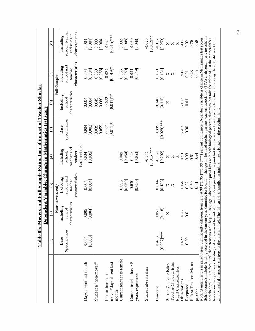
36

T

able

8b:

Mov

ers

and

Ful

l Sam

ple

Est

imat

ion

of im

pact

of

Tea

cher

Sho

cks:

D

epen

dent

Var

iabl

e: C

hang

e in

Mat

hem

atic

s te

st s

core

(1)

(2)

(3)

(4)

(5)

(6)

(7)

(8)

N

on-m

over

s on

ly

Full

-Sam

ple

B

ase

Spec

ific

atio

n In

clud

ing

scho

ol

char

acte

rist

ics

Incl

udin

g sc

hool

and

te

ache

r ch

arac

teri

stic

s

Incl

udin

g sc

hool

, te

ache

r an

d st

uden

t ch

arac

teri

stic

s

Bas

e sp

ecif

icat

ion

In

clud

ing

scho

ol

char

acte

rist

ics

Incl

udin

g sc

hool

and

te

ache

r ch

arac

teri

stic

s

Incl

udin

g sc

hool

, tea

cher

an

d st

uden

t ch

arac

teri

stic

s

Day

s ab

sent

last

mon

th

0.00

4 [0

.003

] 0.

005

[0.0

04]

0.00

4 [0

.004

] 0.

004

[0.0

05]

0.00

4 [0

.003

] 0.

004

[0.0

04]

0.00

4 [0

.004

] 0.

003

[0.0

04]

Stud

ent a

“no

n-m

over

”

0.

039

[0.0

59]

0.04

9 [0

.060

] 0.

059

[0.0

68]

0.09

3 [0

.064

]

Inte

ract

ion:

non

-m

over

*day

s ab

sent

last

m

onth

-0.0

21

[0.0

11]*

-0

.022

[0

.011

]**

-0.0

37

[0.0

19]*

-0

.042

[0

.015

]***

Cur

rent

teac

her

is f

emal

e

0.

053

[0.0

59]

0.04

9 [0

.054

]

0.

036

[0.0

60]

0.03

2 [0

.048

]

Cur

rent

teac

her

has

> 5

ye

ars

expe

rien

ce

-0.0

30

[0.0

50]

-0.0

43

[0.0

53]

-0.0

41

[0.0

49]

-0.0

50

[0.0

48]

Stud

ent a

bsen

teei

sm

-0

.041

[0

.015

]***

-0.0

28

[0.0

12]*

*

Con

stan

t 0.

403

[0.0

27]*

**

0.05

1 [0

.118

] 0.

014

[0.1

36]

-0.2

65

[0.2

92]

0.39

9 [0

.028

]***

0.

148

[0.1

15]

0.15

0 [0

.131

] -0

.137

[0

.259

]

Scho

ol C

hara

cter

istic

s

X

X

X

X

X

X

T

each

er C

hara

cter

isti

cs

X

X

X

X

Pup

il C

hara

cter

isti

cs

X

X

Obs

erva

tions

16

27

1627

14

56

1051

22

04

2187

19

47

1419

R

-squ

ared

0.

00

0.01

0.

02

0.03

0.

00

0.01

0.

01

0.02

F

-Tes

t Tea

cher

s M

atte

r

0.

50

0.61

0.

43

0.70

pr

ob>

F

0.

61

0.54

0.

65

0.50

N

ote:

Sta

ndar

d er

rors

in p

aren

thes

es. S

igni

fica

ntly

dif

fere

nt f

rom

zer

o at

90

(*);

95

(**)

; 99

(***

) pe

rcen

t con

fide

nce.

Dep

ende

nt v

aria

ble

is c

hang

e in

Mat

hem

atic

s te

st s

core

s.

Sch

ool c

ontr

ols

incl

ude

fund

ing

rece

ived

in th

e cu

rren

t yea

r, d

umm

ies

for

loca

tion

, cha

nges

in th

e he

ad te

ache

r, p

aren

ts te

ache

rs a

ssoc

iati

on (

PT

A)

chai

rper

son,

pri

vate

sch

ools

an

d ch

ange

s in

PT

A f

ees

Pup

il c

hara

cter

isti

cs in

clud

e pu

pil s

ex, a

ge, w

heth

er th

e pu

pil l

ives

wit

h bo

th b

iolo

gica

l par

ents

, dum

mie

s th

at ta

ke th

e va

lue

of 1

if th

e m

othe

r/fa

ther

ha

ve m

ore

than

pri

mar

y sc

hool

ing

and

a m

easu

re o

f ho

useh

old

wea

lth.

F-t

est p

erfo

rms

the

join

t tes

t tha

t cur

rent

and

pas

t tea

cher

cha

ract

eris

tics

are

sig

nifi

cant

ly d

iffe

rent

fro

m

zero

. Sta

ndar

d er

rors

are

clu

ster

ed a

t the

teac

her

leve

l. T

he f

ull s

ampl

e of

pup

ils

that

took

bot

h te

sts

is u

sed

in th

ese

esti

mat

ions

.

37

Tab

le 9

: E

stim

ated

Im

pact

of

Tea

cher

Sho

cks

on L

earn

ing

Gai

ns u

sing

Mat

ched

Sam

ple

(1

) (2

) (3

) (4

)

Eng

lish

E

ngli

sh: C

urre

nt a

nd

Pas

t-T

each

er c

ontr

ols

Mat

hem

atic

s M

athe

mat

ics:

C

urre

nt a

nd P

ast-

Tea

cher

Con

trol

s N

on-m

over

s 0.

007

[0.0

78]

0.01

5 [0

.086

] 0.

023

[0.0

69]

0.02

5 [0

.074

]

Day

s A

bsen

t Las

t Mon

th

0.00

2 [0

.006

] 0.

008

[0.0

08]

0.00

3 [0

.005

] 0.

005

[0.0

05]

Non

-Mov

ers*

Day

s A

bsen

t in

Las

t Mon

th

-0.0

39

[0.0

21]*

-0

.044

[0

.022

]**

-0.0

26

[0.0

18]

-0.0

30

[0.0

19]

Con

stan

t 0.

531

[0.1

39]*

**

0.47

7 [0

.278

]*

0.20

5 [0

.149

] 0.

309

[0.2

42]

Oth

er C

ontr

ols

X

X

X

X

Cur

rent

Tea

cher

Con

trol

s X

X

X

X

P

ast T

each

er C

ontr

ols

X

X

Obs

erva

tions

15

06

980

1506

98

0 R

-squ

ared

0.

02

0.02

0.

01

0.01

F

-Tes

t Tea

cher

s M

atte

r 1.

85

0.82

0.

47

0.60

pr

ob>

F 0.

14

0.55

0.

70

0.73

N

ote:

Sta

ndar

d er

rors

in p

aren

thes

es. S

igni

fica

ntly

dif

fere

nt f

rom

zer

o at

90

(*);

95

(**)

; 99

(***

) pe

rcen

t con

fide

nce.

Dep

ende

nt v

aria

ble

defi

ned

as c

hang

e in

te

st s

core

s in

Eng

lish

or M

athe

mat

ics.

Rep

orte

d co

effi

cien

ts e

stim

ated

fro

m a

reg

ress

ion

of c

hang

es in

test

sco

res

on d

ays

abse

nt a

nd p

rovi

nce

dum

mie

s. C

urre

nt

and

Pas

t Tea

cher

con

trol

s in

clud

e te

ache

r ge

nder

, a d

umm

y fo

r 5

or m

ore

year

s of

teac

hing

exp

erie

nce

and

the

poss

essi

on o

f a

teac

hing

cer

tifi

cate

. Oth

er c

ontr

ols

incl

ude

fund

ing

rece

ived

in th

e cu

rren

t yea

r, d

umm

ies

for

loca

tion

, cha

nges

in th

e he

ad te

ache

r, p

aren

ts te

ache

rs a

ssoc

iati

on (

PTA

) ch

airp

erso

n, p

riva

te s

choo

ls

and

chan

ges

in P

TA

fee

s. F

-tes

t per

form

s th

e jo

int t

est t

hat c

urre

nt a

nd p

ast t

each

er c

hara

cter

isti

cs a

re s

igni

fica

ntly

dif

fere

nt f

rom

zer

o. S

tand

ard

erro

rs a

re

clus

tere

d at

the

teac

her

leve

l. T

he s

ampl

e of

non

-mov

ers

and

mat

ched

mov

ers

that

took

bot

h te

sts

is u

sed

in th

ese

esti

mat

ions

. Mat

chin

g is

don

e us

ing

a pr

open

sity

sco

re e

stim

ated

usi

ng c

hild

and

sch

ool c

hara

cter

istic

s.

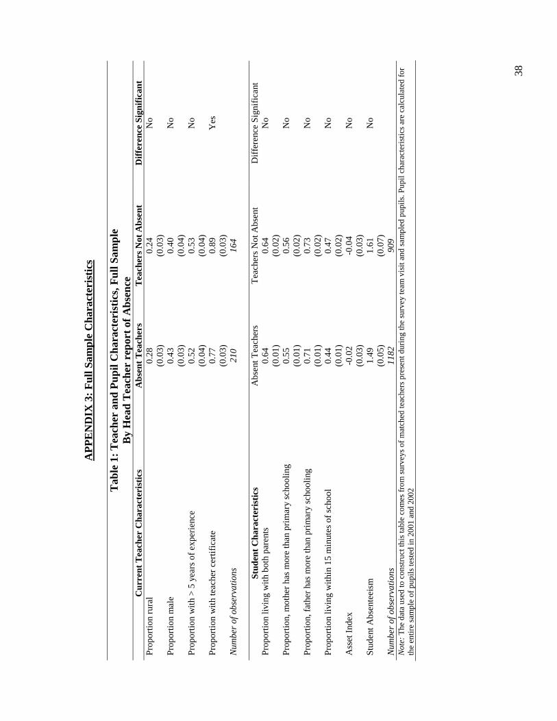
38

AP

PE

ND

IX 3

: F

ull S

ampl

e C

hara

cter

isti

cs

T

able

1:

Tea

cher

and

Pup

il C

hara

cter

isti

cs, F

ull S

ampl

e B

y H

ead

Tea

cher

rep

ort

of A

bsen

ce

Cur

rent

Tea

cher

Cha

ract

eris

tics

A

bsen

t T

each

ers

Tea

cher

s N

ot A

bsen

t D

iffe

renc

e Si

gnif

ican

t P

ropo

rtio

n ru

ral

0.28

(0

.03)

0.

24

(0.0

3)

No

Pro

port

ion

mal

e 0.

43

(0.0

3)

0.40

(0

.04)

N

o

Pro

port

ion

wit

h >

5 y

ears

of

expe

rien

ce

0.52

(0

.04)

0.

53

(0.0

4)

No

Pro

port

ion

wit

h te

ache

r ce

rtif

icat

e 0.

77

(0.0

3)

0.89

(0

.03)

Y

es

Num

ber

of o

bser

vati

ons

210

164

St

uden

t C

hara

cter

isti

cs

Abs

ent T

each

ers

Tea

cher

s N

ot A

bsen

t D

iffe

renc

e S

igni

fica

nt

Pro

port

ion

livin

g w

ith

both

par

ents

0.

64

(0.0

1)

0.64

(0

.02)

N

o

Pro

port

ion,

mot

her

has

mor

e th

an p

rim

ary

scho

olin

g 0.

55

(0.0

1)

0.56

(0

.02)

N

o

Pro

port

ion,

fat

her

has

mor

e th

an p

rim

ary

scho

olin

g 0.

71

(0.0

1)

0.73

(0

.02)

N

o

Pro

port

ion

livin

g w

ithi

n 15

min

utes

of

scho

ol

0.44

(0

.01)

0.

47

(0.0

2)

No

Ass

et I

ndex

-0

.02

(0.0

3)

-0.0

4 (0

.03)

N

o

Stud

ent A

bsen

teei

sm

1.49

(0

.05)

1.

61

(0.0

7)

No

Num

ber

of o

bser

vati

ons

1182

90

9

Not

e: T

he d

ata

used

to c

onst

ruct

this

tabl

e co

mes

fro

m s

urve

ys o

f m

atch

ed te

ache

rs p

rese

nt d

urin

g th

e su

rvey

team

vis

it a

nd s

ampl

ed p

upil

s. P

upil

cha

ract

eris

tics

are

cal

cula

ted

for

the

enti

re s

ampl

e of

pup

ils

test

ed in

200

1 an

d 20

02