Decoding the Pricing of Uncertainty Shocks*

Zhanhui Chen Michael Gallmeyer Baek-Chun Kim§

July 2021

Abstract

Uncertainty affects business cycles and asset prices. We estimate firm-level productivity and

decompose total uncertainty risk measured as cross-sectional productivity dispersion into macro

uncertainty (an aggregate component) and micro uncertainty (an idiosyncratic component).

We find that macro uncertainty is strongly countercyclical and priced among stocks, but micro

uncertainty is acyclical and not priced. Moreover, we show that the expected investment growth

factor proposed in Hou, Mo, Xue, and Zhang (2021) captures macro uncertainty risk which helps

us understand the success of the q5-model.

JEL classification: G12, E20, E24, E32, D24

Keywords: macro uncertainty, micro uncertainty, expected investment growth factor

*We thank David Chapman, Bernard Herskovic, Sheisha Kulkarni, Jun Li, Robert McDonald, Haitao Mo, YanXu, Chen Xue, and seminar participants at the 2021 AFA Annual Meeting, the UBC Summer Finance Conference,the University of Melbourne, and the Hong Kong Joint Finance Research Workshop for helpful comments.

Department of Finance, School of Business and Management, Room 5075 Lee Shau Kee Business Building, HongKong University of Science and Technology, Clear Water Bay, Kowloon, Hong Kong. Tel.: +852-2358-7670; Fax:+852-2358-1749; E-mail: chenzhanhui@ust.hk.

McIntire School of Commerce, University of Virginia, Rouss & Robertson Halls, East Lawn, Office 323, Char-lottesville, VA 22904 and and the Faculty of Business and Economics, University of Melbourne. Tel.: 434-243-4043;E-mail: mgallmeyer@virginia.edu.

§Department of Finance, School of Management, Room 637 Jiageng Building 2, Xiamen University, China. E-mail:baekchun@e.xmu.edu.cn.

Uncertainty coincides with business cycles (Bloom, 2009; Fernandez-Villaverde et al., 2015;

Basu and Bundick, 2017; Bloom et al., 2018),1 and affects asset prices as well (Bansal and Yaron,

2004; Segal et al., 2015; Bali et al., 2017, 2020). Uncertainty includes both macroeconomic and

microeconomic components. Previous studies such as Bloom et al. (2018) use both components to

match business cycle fluctuations theoretically by assuming a significant role for micro uncertainty

relative to macro uncertainty under the assumption both are driven by a common latent process.

However, these two uncertainty measures seem to be distinct as discussed in Kozeniauskas et al.

(2018). Given their difference is understudied, this paper aims to fill this gap by examining these

two components from an asset pricing perspective. We first estimate firm-level productivity and

then decompose uncertainty risk measured as cross-sectional productivity dispersion into macro

uncertainty (an aggregate component) and micro uncertainty (an idiosyncratic component). We find

that macro uncertainty is strongly countercyclical and priced among stocks, but micro uncertainty

is acyclical and not priced. This challenges the importance of micro uncertainty over business

cycles.

To motivate our empirical work, we consider a simple production economy with time-varying

productivity volatility to study the impact of uncertainty on consumption, investment, and asset

prices. Due to precautionary savings motives, agents reduce their consumption when uncertainty

increases. Given the resource constraint and convex adjustment costs (i.e., no fixed costs), firms

increase investment when uncertainty increases,2 which implies a lower expected investment growth

rate and lower expected returns. Therefore, expected returns increase with expected investment

growth via an uncertainty channel. We test this prediction with the expected investment growth

(EG) factor proposed in the q5-model of Hou et al. (2021). We find evidence that the pricing

power of the EG factor is driven by macro uncertainty risk. This provides an alternative way to

understand the success of the EG factor and the q5-model.

Empirically, we follow Bloom (2014) to measure uncertainty as time-varying volatilities (see,

e.g., Bloom, 2009; Jurado et al., 2015; Bloom et al., 2018). Uncertainty contains two components

— macro and micro uncertainty shocks. Macro uncertainty refers to the aggregate uncertainty

in the economy, which is often measured over an aggregate index such as aggregate productivity

1The causality is unclear, as Bloom et al. (2018) discuss. Uncertainty might lead to business fluctuations. Alterna-tively, uncertainty may arise endogenously from business cycles. Many papers find that the cross-sectional dispersionsof firm- or establishment-level variables, like productivity, output, prices, employment, and business forecasts, appearto be counter cyclical (Bloom, 2009; Bachmann and Bayer, 2013; Bachmann et al., 2013; Bachmann and Bayer, 2014;Kehrig, 2015; Bloom et al., 2018; David et al., 2018).

2Investment could decrease with uncertainty initially by adding fixed adjustment costs (see, e.g., Bloom et al.(2018)).

1

or stock market volatility. Macro uncertainty is countercyclical (Bloom et al., 2018) and its asset

pricing power is well accepted as it changes investors’ future consumption growth and investment

opportunities (Bansal and Yaron, 2004; Segal et al., 2015; Bali et al., 2017, 2020).

In contrast, micro uncertainty captures uncertainty about idiosyncratic volatility. Although

idiosyncratic volatility might appear to be priced due to missing factors or a common volatility

factor as discussed in Chen and Petkova (2012) and Herskovic et al. (2016), it is unclear whether

micro uncertainty is priced. In particular, the empirical measure of micro uncertainty used often

clouds the results. For example, Bloom et al. (2018) use the cross-sectional dispersion of micro-level

data (e.g., establishment- or firm-level productivity) to measure micro uncertainty and find micro

uncertainty is countercyclical, suggesting a pricing role for micro uncertainty. However, such a

micro uncertainty measure is contaminated with macro uncertainty, since micro level productivity

contains both systematic and idiosyncratic productivity.3 This calls for a clean measurement of

micro uncertainty to help us understand whether micro uncertainty matters.

Guided by this observation, we use firm-level data to differentiate micro and macro economic

uncertainty in two steps. First, we estimate firm-level total factor productivity (TFP) following

Olley and Pakes (1996) and Imrohoroglu and Tuzel (2014) at an annual frequency. Total uncertainty

is measured as the cross-sectional standard deviation of these TFP shocks. Second, we apply

an asymptotic principal component analysis as in Connor and Korajczyk (1987), Herskovic et al.

(2016), and Chen et al. (2018) to estimate the systematic and idiosyncratic TFP components across

all firms. We identify six principal components of productivity shocks.4 Macro (Micro) uncertainty

is measured as the cross-sectional standard deviation of systematic (idiosyncratic) productivity

shocks. Figure 1 shows macro uncertainty (total uncertainty) is countercyclical, with a correlation

coefficient of -0.26 (-0.10) with industrial production growth. Micro uncertainty is almost acyclical

(the correlation coefficient with the industrial production growth is 0.004). That is, uncertainty

is high during recessions and this is driven mainly by the macro uncertainty. This suggests that

macro uncertainty and not micro uncertainty relates to business cycles.

We first use the annual non-tradable uncertainty factor and run Fama-MacBeth two-pass re-

gressions to test its pricing power, by matching stock returns with lagged uncertainty risk. We

augment seven factor models with the total uncertainty factor, the macro uncertainty factor, or

3Schaab (2020) illustrates that aggregate uncertainty can be transmitted to heterogeneous households via unem-ployment risk and wage volatilities. Therefore, household-level uncertainty also contains macro uncertainty.

4Chen and Kim (2019) show that this decomposition reasonably captures aggregate and idiosyncratic productivityshocks.

2

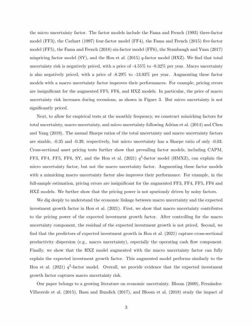
the micro uncertainty factor. The factor models include the Fama and French (1993) three-factor

model (FF3), the Carhart (1997) four-factor model (FF4), the Fama and French (2015) five-factor

model (FF5), the Fama and French (2018) six-factor model (FF6), the Stambaugh and Yuan (2017)

mispricing factor model (SY), and the Hou et al. (2015) q-factor model (HXZ). We find that total

uncertainty risk is negatively priced, with a price of -4.55% to -9.32% per year. Macro uncertainty

is also negatively priced, with a price of -8.29% to -13.93% per year. Augmenting these factor

models with a macro uncertainty factor improves their performances. For example, pricing errors

are insignificant for the augmented FF5, FF6, and HXZ models. In particular, the price of macro

uncertainty risk increases during recessions, as shown in Figure 3. But micro uncertainty is not

significantly priced.

Next, to allow for empirical tests at the monthly frequency, we construct mimicking factors for

total uncertainty, macro uncertainty, and micro uncertainty following Adrian et al. (2014) and Chen

and Yang (2019). The annual Sharpe ratios of the total uncertainty and macro uncertainty factors

are sizable, -0.35 and -0.39, respectively, but micro uncertainty has a Sharpe ratio of only -0.03.

Cross-sectional asset pricing tests further show that prevailing factor models, including CAPM,

FF3, FF4, FF5, FF6, SY, and the Hou et al. (2021) q5-factor model (HMXZ), can explain the

micro uncertainty factor, but not the macro uncertainty factor. Augmenting these factor models

with a mimicking macro uncertainty factor also improves their performance. For example, in the

full-sample estimation, pricing errors are insignificant for the augmented FF3, FF4, FF5, FF6 and

HXZ models. We further show that the pricing power is not spuriously driven by noisy factors.

We dig deeply to understand the economic linkage between macro uncertainty and the expected

investment growth factor in Hou et al. (2021). First, we show that macro uncertainty contributes

to the pricing power of the expected investment growth factor. After controlling for the macro

uncertainty component, the residual of the expected investment growth is not priced. Second, we

find that the predictors of expected investment growth in Hou et al. (2021) capture cross-sectional

productivity dispersion (e.g., macro uncertainty), especially the operating cash flow component.

Finally, we show that the HXZ model augmented with the macro uncertainty factor can fully

explain the expected investment growth factor. This augmented model performs similarly to the

Hou et al. (2021) q5-factor model. Overall, we provide evidence that the expected investment

growth factor captures macro uncertainty risk.

Our paper belongs to a growing literature on economic uncertainty. Bloom (2009), Fernandez-

Villaverde et al. (2015), Basu and Bundick (2017), and Bloom et al. (2018) study the impact of

3

uncertainty on business cycles. Kozeniauskas et al. (2018) show that various macro uncertainty,

micro uncertainty, and higher-order uncertainty measures are distinct and some are statistically

uncorrelated. Dew-Becker and Giglio (2020) show that cross-sectional uncertainty, measured using

option data, does not forecast overall economic activity as well as aggregate uncertainty.

Other works examine the asset pricing implications of aggregate uncertainty shocks. For ex-

ample, Bansal and Yaron (2004) consider the equity premium implied by the conditional volatility

of consumption growth. Bekaert et al. (2009) show that economic uncertainty contributes to the

term structure and countercyclical volatility of asset returns. Hartzmark (2016) shows that higher

uncertainty leads to lower interest rates. Bali and Zhou (2016) show that economic uncertainty,

proxied by the variance risk premium, is significantly priced. Dew-Becker et al. (2017), Berger et al.

(2019), and Dew-Becker et al. (2019) differentiate between uncertainty and realized variance using

data from equity derivative markets. They show that realized variance has a negative premium,

while aggregate uncertainty carries a zero or a positive premium. Segal et al. (2015) differentiate

good and bad uncertainty arising from positive and negative industrial production growth. Alfaro

et al. (2019) consider real and financial frictions to amplify the impacts of uncertainty shocks.

Schaab (2020) considers the transmission and interaction of aggregate uncertainty and household-

level uncertainty. More closely related to our work, Bali et al. (2017) and Bali et al. (2020) find that

macroeconomic uncertainty is priced in the cross section of stocks and corporate bonds using the

Jurado et al. (2015) uncertainty index. Herskovic et al. (2020) consider uncertainties of aggregate

consumption growth and firm-specific productivity shocks, and show that the former drives size

and value premia while the latter contributes to the equity premium. Our paper contributes to this

literature by differentiating macro and micro uncertainty and shows that micro uncertainty does

not matter for asset prices.

Our paper also follows in the tradition of the production-based asset pricing literature such as

Cochrane (1991), Cochrane (1996), Berk et al. (1999), Zhang (2005), and Liu et al. (2009). The

neoclassical theory of investment stresses that production risks drive stock risks. Hou et al. (2015)

and Hou et al. (2021) construct pricing factors based on firm investment, profitability, and expected

investment growth.5 Our paper adds to this literature by studying the role of uncertainty shocks.

Lastly, our paper also contributes to the large literature on the empirical performance of cross-

sectional asset pricing factor models. For example, Fama and French (2015) construct a five-factor

5Li et al. (2020) consider the impact of investment lags and show that aggregate expected investment growthnegatively predicts future market returns due to firms’ investment plans.

4

model based on the dividend discount model/surplus clean accounting method, including a market

factor, a size factor, a value factor, an investment factor, and a profitability factor. Fama and

French (2018) further add a momentum factor to their five-factor model. Hou et al. (2015) propose

a q-factor model motivated by the q-theory of investment, including a market factor, a size factor, an

investment factor, and a profitability factor. Hou et al. (2021) further add an expected investment

growth factor to their q-factor model to create their q5 model. Stambaugh and Yuan (2017) study a

four-factor model, which includes a market factor, a size factor, and two mispricing factors. Overall,

these factor models perform well in explaining a host of anomalies. Our paper suggests that the

macro uncertainty factor is missing from most models with the notable exception of the Hou et al.

(2021) q5 model as we show that macro uncertainty risk contributes to the pricing power of their

expected investment growth factor in the q5 model.

The rest of the paper proceeds as follows. Section 1 presents a production-based model to ex-

plore the linkage between uncertainty shocks, expected investment growth, and asset prices. Section

2 describes the data and the procedures used for estimating various uncertainty measures and their

estimates. Section 3 presents cross-sectional asset pricing tests, using non-tradable uncertainty

factors. Section 4 tests the pricing power of the uncertainty factors, using mimicking portfolios.

Section 5 explores the relationship between the macro uncertainty factor and the expected invest-

ment growth factor. Finally, Section 6 concludes.

1. Uncertainty shocks, expected investment growth, and asset

prices: A motivating model

We consider a simple partial equilibrium production economy to illustrate the impact of un-

certainty shocks on expected investment growth and asset prices.6 We assume an all-equity repre-

sentative firm which operates in discrete time with an infinite horizon. The firm generates output

according to a constant returns to scale production function: Yt = XtKt. Yt and Xt are the firm’s

output and total factor productivity at time t, respectively. Kt is the productive capital at the

beginning of time t.

6See Appendix A for a general equilibrium model.

5

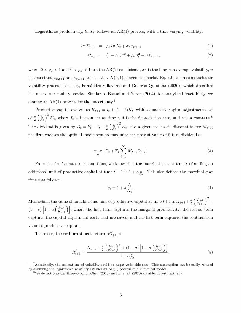
Logarithmic productivity, lnXt, follows an AR(1) process, with a time-varying volatility:

lnXt+1 = ρx lnXt + σt εx,t+1, (1)

σ2t+1 = (1− ρσ)σ2 + ρσσ

2t + υ εσ,t+1, (2)

where 0 < ρx < 1 and 0 < ρσ < 1 are the AR(1) coefficients, σ2 is the long-run average volatility, υ

is a constant, εx,t+1 and εσ,t+1 are the i.i.d. N(0, 1) exogenous shocks. Eq. (2) assumes a stochastic

volatility process (see, e.g., Fernandez-Villaverde and Guerron-Quintana (2020)) which describes

the macro uncertainty shocks. Similar to Bansal and Yaron (2004), for analytical tractability, we

assume an AR(1) process for the uncertainty.7

Productive capital evolves as Kt+1 = It + (1 − δ)Kt, with a quadratic capital adjustment cost

of a2

(ItKt

)2Kt, where It is investment at time t, δ is the depreciation rate, and a is a constant.8

The dividend is given by Dt = Yt − It − a2

(ItKt

)2Kt. For a given stochastic discount factor Mt+i,

the firm chooses the optimal investment to maximize the present value of future dividends:

maxIt

Dt + Et∞∑i=1

[Mt+iDt+i]. (3)

From the firm’s first order conditions, we know that the marginal cost at time t of adding an

additional unit of productive capital at time t + 1 is 1 + a ItKt

. This also defines the marginal q at

time t as follows:

qt ≡ 1 + aItKt. (4)

Meanwhile, the value of an additional unit of productive capital at time t+1 is Xt+1 + a2

(It+1

Kt+1

)2+

(1 − δ)[1 + a

(It+1

Kt+1

)], where the first term captures the marginal productivity, the second term

captures the capital adjustment costs that are saved, and the last term captures the continuation

value of productive capital.

Therefore, the real investment return, RIt+1, is

RIt+1 =Xt+1 + a

2

(It+1

Kt+1

)2+ (1− δ)

[1 + a

(It+1

Kt+1

)]1 + a It

Kt

. (5)

7Admittedly, the realizations of volatility could be negative in this case. This assumption can be easily relaxedby assuming the logarithmic volatility satisfies an AR(1) process in a numerical model.

8We do not consider time-to-build. Chen (2016) and Li et al. (2020) consider investment lags.

6

Cochrane (1991) and Restoy and Rockinger (1994) show that stock returns equal real investment

returns when production is constant returns to scale. Therefore, Eq. (5) also computes stock

returns, Rt+1.

Next, we consider a log-linearized version of the economy. Let Vt denote logarithmic deviations

of variable V from its steady state. Given the three state variables (i.e., productivity Xt, productive

capital Kt, and uncertainty σ2t ), the optimal investment can be approximated as:

It = I0 + IxXt + IkKt + Iσσ2t , (6)

where the coefficients satisfy I0 > 0, Ix > 0, Ik = 1 (due to constant returns to scale production),

and Iσ > 0 (see details in Appendix A).9 Log-linearizing Eq. (5) approximates the expected return

as

Et[Rt+1] = (h− 1)I0 + hIσ(1− ρσ)σ2

+

[h

aδρx + hIxρx −

aδ

1 + aδIx

]Xt︸ ︷︷ ︸

prductivity shock

+

[hρσ −

aδ

1 + aδ

]Iσσ

2t︸ ︷︷ ︸

uncertainty shock

, (7)

where h = aδ2−a

2δ2+(a−1)δ

. In this economy, two fundamental risks drive expected stock returns,

including the productivity shock and the uncertainty shock. For example, higher productivity

leads to higher expected returns as productivity is persistent. Also, we see that the uncertainty

shock, σ2t in Eq. (7), affects stock returns. Since 0 < h < aδ

1+aδ and 0 < ρσ < 1, the expected return

decreases with the uncertainty shock. Clearly, firm characteristics such as the investment factor

(as shown in Eq. (6)) and the profitability factor might incorporate some information about these

two fundamental risks.

Eq. (4) suggests that qt is a sufficient statistic of the rate of investment ItKt

. Following Lettau

and Ludvigson (2002), expected investment growth is proportional to the expected growth rate of

q, as follows

Et

[ˆIt+1

Kt+1− ItKt

]=

1 + aδ

aδEt [qt+1 − qt]

= Iσ(1− ρσ)σ2 + (ρx − 1) IxXt + (ρσ − 1) Iσσ2t . (8)

9This implies that investment increases with uncertainty, because consumption decreases for precautionary reasons.Bloom et al. (2018) use nonconvex adjustment costs (i.e., fixed costs) of capital investment and labor hiring so thatinvestment decreases with uncertainty initially.

7

Therefore, expected investment growth also captures these two fundamental risks. For example,

since Iσ > 0 and 0 < ρσ < 1, the expected investment growth decreases with uncertainty shocks

(σ2t ). Taking Eq. (7) and (8) together, we see that expected investment growth captures uncertainty

shocks and therefore it captures expected stock returns. That is, the expected return increases with

expected investment growth via the uncertainty channel.

The above results can be easily extended to a cross section of firms which allows for firm-specific

productivity shocks. For example, we can specify the production function of firm i as XtAi,tKi,t,

where Ai,t and Ki,t are firm i’s specific productivity and productive capital. We can embed micro

uncertainty into Ai,t. However, whether the micro uncertainty is priced or not is an empirical

question, which we explore below.

2. Estimating uncertainty shocks

Following Bloom et al. (2018), we first estimate firm-level total factor productivity (TFP). The

cross-sectional dispersion of TFP shocks is then used as a total uncertainty measure. Next, we

decompose total uncertainty into macro and micro uncertainty.

2.1. Estimating firm-level TFP and the total uncertainty

We closely follow Olley and Pakes (1996) and Imrohoroglu and Tuzel (2014) to estimate firm-

level TFP. Olley and Pakes (1996) address two endogeneity issues involving TFP estimation. First,

since input factors (labor and capital stock) are contemporaneously correlated, there is a simul-

taneity bias. They estimate the production function parameters for each input factor separately

to address this bias. Second, there is a selection bias, because firms exit or enter the markets

depending on their productivity. Olley and Pakes (1996) assume TFP is a function of a firm’s sur-

vival probability and include that in the TFP estimation. Olley and Pakes (1996) further assume

that (1) TFP is a first-order Markov process; (2) physical capital is predetermined after TFP is

observed; and (3) investment reflects information about TFP. Imrohoroglu and Tuzel (2014) apply

Olley and Pakes (1996) to estimate firm-level TFP. We follow their estimation procedures with

some modifications.

Assume a Cobb-Douglas production function:

Yit = ZitLβLit K

βKit , (9)

8

where Yit, Zit, Lit, and Kit are value-added, productivity, labor, and capital stock of a firm i at

time t. The productivity contains both systematic and idiosyncratic components. Next, we scale

the production function by its capital stock and take logarithms. We perform this scaling for three

reasons. First, since TFP is the residual term, it is highly correlated with firm size. Second, the

scaling avoids estimating the capital coefficient directly. Third, it mitigates an upward bias in the

labor coefficient. Eq. (9) can be rewritten as

LogYitKit

= βLLogLitKit

+ (βK + βL − 1)LogKit + LogZit. (10)

Denote Log YitKit, Log Lit

Kit, LogKit, and LogZit as ykit, lkit, kit, and zit. Also, let βL and (βK+βL−1)

be βl and βk. Rewrite Eq. (10) as follows:

ykit = βllkit + βkkit + zit. (11)

We estimate the labor coefficient (βl) and capital coefficient (βk) using linear regressions. Then,

the logarithmic TFP, zit, is ykit − βllki,t − βkkit. We estimate TFP using a 5-year rolling window.

Similar to Bloom et al. (2018), we define the cross-sectional standard deviation of TFP at time

t as the cross-sectional TFP dispersion, i.e., total uncertainty (denoted as UNC). We take the

first difference of this cross-sectional TFP dispersion as the total uncertainty shock (denoted as

∆UNC). Note that this firm-level TFP dispersion is often used as micro uncertainty in the litera-

ture. However, as we show below, this measure contains macro uncertainty also.

We use annual Compustat data to estimate TFP for common stocks from the NYSE, Amex,

and Nasdaq. To obtain stable estimates, following Bloom et al. (2018), we assume all firms follow

the same production function. This will introduce some noise in our estimates, since production

functions may vary across industries and over time. However, as we decompose total uncertainty

into micro and macro components, we expect the measurement errors to be small, especially for

macro uncertainty. We include all firms except for financial and utility firms (four-digit SIC between

6000 - 6999 and between 4900 - 4999).10 We exclude firms with assets or sales below 1 million or

year-end stock price lower than $5. Following Chen and Chen (2012), we also exclude firms with

asset or sales growth rate exceeding 100% to avoid potential business discontinuities that might be

caused by mergers and acquisitions. The sample period is from 1966 to 2016. The TFP estimates

are from 1972 to 2016. The estimated labor coefficient βl is 0.56 and the estimated capital coefficient

10The results are qualitatively similar if we restrict our sample to manufacturing firms only.

9

βk is 0.38. These estimates are similar to those reported in Olley and Pakes (1996), and are in line

with neoclassical models. For example, Bloom et al. (2018) assume that the labor coefficient is 2/3

and the capital coefficient is 1/3. During our sample period, the production technology is slightly

decreasing returns-to-scale (βl + βk = 0.94). See Appendix B for more details.

2.2. Estimating macro and micro uncertainty

Following Herskovic et al. (2016), we decompose firm-level TFP into systematic and idiosyn-

cratic components via the asymptotic principal component analysis of Connor and Korajczyk

(1987). This allows us to separate systematic and idiosyncratic productivity. TFP estimates for N

firms over time T , denoted as TFPNT , can be decomposed into k principal components:

TFPNT = BNk × PCkT + εNT , (12)

where TFP is an N × T matrix of TFP, B is an N × k matrix of the sensitivities to aggregate

TFP shocks, PC is a k × T matrix of systematic TFP shocks, and ε is an N × T matrix of the

idiosyncratic TFP shock. Next, we calculate Ω = 1N TFP

TTFP and estimate the eigenvector of Ω.

We multiply each element of the eigenvectors with 1√T

to obtain unit standard deviations.

To more precisely estimate the systematic TFP components (PC), we use firms with more than

10 years of data. We choose six principal components (k = 6), following Chen and Kim (2019) as

they find that (1) six principal components explain more than 50% of firm-level TFP; (2) there is a

positive contemporaneous correlation between stock returns and systematic TFP growth; and (3)

only the volatility of systematic productivity positively predicts expected stock returns while the

idiosyncratic volatility cannot. These findings suggest that six principal components reasonably

approximate the systematic productivity shocks.

After we estimate systematic TFP growth and idiosyncratic TFP growth, we calculate the cross-

sectional standard deviations of systematic TFP growth and idiosyncratic TFP growth, which are

defined as macro uncertainty and micro uncertainty here. Then, we take their first differences to

compute macro and micro uncertainty shocks, denoted as ∆UNCma and ∆UNCmi, respectively.

Although idiosyncratic productivity is not priced, it is unclear if micro uncertainty is priced, because

micro uncertainty maybe relate to some additional state variables.

10

2.3. Uncertainty estimates

Panel A of Table 1 shows that TFP growth (∆TFP ) has a mean of 0.01 and a standard deviation

of 0.21. TFP growth varies over both the cross section and the time series. The next three rows

present descriptive statistics for uncertainty shocks. Total uncertainty (∆UNC) has a mean of 0.00

with a standard deviation of 0.05. Macro uncertainty (∆UNCma) has a larger standard deviation

of 0.07, while micro uncertainty (∆UNCmi) only has a standard deviation of 0.03.

Figure 1 shows the time series of the uncertainty shocks and industrial production growth

(IP ), including total uncertainty, macro uncertainty, and micro uncertainty. We apply the band-

pass filter of Christiano and Fitzgerald (2003) to these series. Similar to findings in Bloom et al.

(2018), total uncertainty (UNC) is countercyclical, with a correlation coefficient of -0.10 with

IP growth.11 Therefore, uncertainty is high during recessions. Moreover, we see that macro un-

certainty (UNCma) is strongly countercyclical, with a correlation coefficient of -0.26, but micro

uncertainty (UNCmi) is barely correlated with IP growth, with a correlation coefficient of 0.004.

Total uncertainty being countercyclical is mainly due to macro uncertainty.

In Figure 2, we plot the cross-sectional standard deviation of stock returns with various un-

certainty measures. We decompose the stock return into systematic and idiosyncratic components

by regressing annual stock returns with the Carhart (1997) four-factor model. We use the pre-

dicted stock return as the systematic component and residuals as the idiosyncratic component.

We calculate the cross-sectional standard deviations of stock returns and the two components in

each year, denoted as RD, RDsys, and RDidio. Panels (a) and (b) of Figure 2 show that the

total uncertainty and macro uncertainty track the cross-sectional return dispersions quite well. For

example, the correlation coefficients between UNC and RD, RDsys, and RDidio are 0.53, 0.56,

and 0.59, respectively. The correlation coefficients between UNCma and RD, RDsys, and RDidio

are 0.56, 0.57, and 0.55, respectively. However, Panel (c) of Figure 2 shows that UNCmi is much

less correlated with RD and RDsys (the correlation coefficients are -0.04 and -0.12, respectively).

Figure 2 shows that our uncertainty measures are reasonably estimated and comove with the stock

return dispersions.

Panel B of Table 1 provides the annual correlation coefficients between the uncertainty measures

11Using the detailed Census microdata of manufacturing establishments from 1972 to 2011, Bloom et al. (2018)find that TFP dispersion is negatively correlated with GDP growth with a correlation coefficient of -0.45. Our TFPdispersion measure differs from Bloom et al. (2018) in three ways. First, their TFP is establishment-level while ourTFP is firm-level. Second, they only cover manufacturing establishments but our sample includes all firms exceptfinancials and utilities. Third, they estimate TFP following Foster et al. (2001).

11

and cross-sectional pricing factors. We consider 11 pricing factors, including: (1) six factors in Fama

and French (2018), which are the market portfolio (MKT), the size factor (SMB), the value factor

(HML), the investment factor (CMA), the profitability factor (RMW), and the momentum factor

(UMD); (2) five factors from Hou et al. (2021), i.e., the market portfolio (MKT), the size factor

(QME), the investment factor (QIA), the profitability factor (QROE), and the expected investment

growth factor (EG); and (3) the univariate mispricing factor (MIS) from Stambaugh and Yuan

(2017).

Consistent with the predictions in Section 1, Panel B shows that total uncertainty (∆UNC)

is positively related to the expected investment growth factor (EG) (a correlation coefficient of

0.29). We also see that macro uncertainty (∆UNCma) is highly correlated with ∆UNC, with

a correlation coefficient of 0.87. This suggests that total uncertainty is mainly driven by macro

uncertainty. Also, ∆UNCma has a pronounced correlation coefficient with EG, 0.25. Third, micro

uncertainty (∆UNCmi) has negative correlations with ∆UNC and ∆UNCma. Also, ∆UNCmi

does not have a strong correlation with EG. Overall, Panel B provides evidence that ∆UNCma

captures most of ∆UNC and both measures have a significant relationship with the EG factor.

2.4. Inspecting the uncertainty decomposition

In this subsection, we validate our uncertainty decomposition in three steps. First, we check

if our macro uncertainty measure reasonably captures aggregate uncertainty. To this end, we

obtain aggregate TFP data from the Federal Reserve Bank of San Francisco and following Bloom

et al. (2018), we define aggregate uncertainty (UNCagg) as the conditional standard deviation

of a GARCH (1,1) on aggregate TFP. Panel A of Table 2 reports the time-series regressions of

aggregate uncertainty on macro uncertainty (UNCma) and micro uncertainty (UNCmi). Macro

uncertainty positively predicts the aggregate uncertainty while micro uncertainty does not. This is

also confirmed by the correlation between uncertainty shocks and VIX. Panel A of Table 1 shows

that total uncertainty and macro uncertainty positively correlate with VIX, with a correlation

coefficient of 0.38 and 0.37, respectively. But the correlation coefficient of micro uncertainty and

VIX is -0.18.

Second, using our TFP estimates, we investigate if total uncertainty is mainly driven by macro

uncertainty. Panel B of Table 2 reports the time-series regressions of ∆UNC against ∆UNCma

and ∆UNCmi. The univariate regression in Column (1) shows that ∆UNCma has a coefficient

of 0.60 (t-statistic=10.11) and the R2 is 0.75. This is not surprising given the high correlation

12

between ∆UNC and ∆UNCma reported in Panel B of Table 1. In Column (2), we add ∆UNCmi

to the regression. The coefficient of ∆UNCmi is 0.53 (t-statistic=3.11) while that of ∆UNCma is

0.73 (t-statistic=9.62). Also, the explanatory power (R2) increases by only 0.06 from Column (1)

to Column (2). Panel B of Table 2 suggests that ∆UNC is mainly driven by ∆UNCma.

3. Pricing of uncertainty shocks: Using annual non-tradable un-

certainty factors

We run Fama-MacBeth two-stage regressions to examine the pricing power of uncertainty shocks

using annual non-tradable uncertainty factors, including total uncertainty, macro uncertainty, and

micro uncertainty. We use 45 portfolios, including 6 size and book-to-market sorted portfolios, 6

size and operating profitability sorted portfolios, 6 size and investment sorted portfolios, 6 size and

momentum sorted portfolios, 6 size and expected investment growth sorted portfolios, 10 operating

accrual sorted portfolios, and 5 Fama-French industry portfolios.12 Following Lewellen et al. (2010),

we add the pricing factors of tested factor models to test assets in order to restrict the price of risk

to be equal to the average factor return. To ensure that uncertainty risk is strictly observable, we

match the uncertainty estimates in year t to test portfolios from July of year t+ 1 to June of year

t+ 2. That is, we match stock returns with lagged uncertainty risks.

We augment the prevailing factor models with the total uncertainty factor, macro uncertainty

factor, or micro uncertainty factor, and compare those to the prevailing factor models. We consider

seven factor models, including the Fama and French (1993) three-factor model (FF3), the Carhart

(1997) four-factor model (FF4), the Fama and French (2015) five-factor model (FF5), the Fama

and French (2018) six-factor model (FF6), the Stambaugh and Yuan (2017) mispricing factor model

(SY), the Hou et al. (2015) q-factor model (HXZ), and the Hou et al. (2021) q5 model (HMXZ).

But we do not augment the Hou et al. (2021) q5 model (HMXZ) since EG and ∆UNCma are

highly correlated. We leave our discussion of the q5 model for Section 5. For example, the macro

uncertainty augmented factor models are as follows:

FF3+∆UNCma:

Rit = γ0 + γMKT βMKT,i + γSMBβSMB,i + γHMLβHML,i + γUNCma βUNCma,i + εit

FF4+∆UNCma:

Rit = γ0 + γMKT βMKT,i + γSMBβSMB,i + γHMLβHML,i + γUMDβUMD,i + γUNCma βUNCma,i + εit

FF5+∆UNCma:

12We download these portfolios from the following websites:http://mba.tuck.dartmouth.edu/pages/faculty/ken.french/index.html; http://global-q.org/index.html

13

Rit = γ0+γMKT βMKT,i+γSMBβSMB,i+γHMLβHML,i+γCMAβCMA,i+γRMW βRMW,i+γUNCma βUNCma,i+

εit

FF6+∆UNCma:

Rit = γ0+γMKT βMKT,i+γSMBβSMB,i+γHMLβHML,i+γCMAβCMA,i+γRMW βRMW,i+γUMDβUMD,i+

γUNCma βUNCma,i + εit

HXZ+∆UNCma:

Rit = γ0 + γMKT βMKT,i + γQMEβQME ,i + γQIA

βQIA,i + γQROEβQROE ,i + γUNCma βUNCma,i + εit

SY+∆UNCma:

Rit = γ0+γMKT βMKT,i+γMISMEβMISME ,i+γMGMT βMGMT,i+γPERF βPERF,i+γUNCma βUNCma,i+

εit

In the first stage, we run the time-series regression of each model to estimate the factor loadings

for each asset using the full sample. In the second stage, we run the cross-sectional regression of

all test assets on the factor loadings each year and then compute the time-series average of the

prices of risk. We adjust the t-statistics following Shanken (1992). We report the adjusted R2

from Jagannathan and Wang (1996). Following Lewellen et al. (2010), we construct a sampling

distribution of the adjusted R2 by bootstrapping the time-series return data and factors by sampling

with replacement to estimate the adjusted R2. We repeat this procedure 10,000 times and report

the 5th and 95th percentiles of the sampling distribution of the adjusted R2. The testing period is

from July 1974 to June 2018.

We report the regression results of the total uncertainty factor in Panel A of Table 3. We

find γUNC is significantly priced across different factor models. The price of total uncertainty risk

ranges from -9.32% to -4.55% per year. Total uncertainty factor also improves model fit. For

example, after adding the total uncertainty factor to FF6, the intercept γ0 becomes insignificant

(t-statistic=1.52) while the adjusted R2 increases from 0.71 to 0.78.

Panel B of Table 3 reports the results using the macro uncertainty factor. First, we see that

macro uncertainty is negatively priced in all models. The price of macro uncertainty risk γUNCma

is sizable, ranging from -13.93% to -8.29% per year across different augmented factor models.

Second, we see that ∆UNCma improves the model performance. For example, the pricing error is

insignificant in FF5+∆UNCma (0.71% per year, t-statistic=1.64) and FF6+∆UNCma (0.58% per

year, t-statistic=1.54) . The results in Panels A and B of Table 3 are similar, which again suggests

that the pricing power of total uncertainty is mainly from macro uncertainty risk. In Panel C of

Table 3, we replace the macro uncertainty factor with the micro uncertainty factor. The price of

micro uncertainty risk is negligible and insignificant.

14

Figure 3 plots the prices of total uncertainty risk (UNC) and macro uncertainty risk (UNCma)

against industrial production growth. The prices of uncertainty risks are computed from the Fama-

French three-factor model augmented with the uncertainty factor. We see that the correlation

between the price of UNC (UNCma) and IP growth is 0.27 (0.25). Therefore, during recessions

(when IP growth is low), uncertainty increases and the price of uncertainty risk becomes more

negative. This is consistent with the explanations in Bali et al. (2017) and Alfaro et al. (2019).

Overall, these results provide evidence that the macro uncertainty factor explains the various

test assets with a significantly negative price of risk, while the micro uncertainty factor does not.

4. Pricing of uncertainty shocks: Mimicking uncertainty factors

In the previous section, we used annual non-tradable uncertainty factors to perform asset pricing

tests. However, their statistical power might be limited by the sample size. We now construct

monthly mimicking portfolios for the uncertainty factors. We use mimicking uncertainty factors as

our main estimates in the rest of the paper as the monthly mimicking factors have more statistical

power and allow us to perform more empirical tests.

4.1. Constructing mimicking uncertainty factors

As the productivity dispersion shocks are annual, to construct monthly mimicking portfolios,

we follow Adrian et al. (2014) and Chen and Yang (2019) by using a projection method. First, we

project the uncertainty shocks (∆UNC) onto a set of annual base asset returns:

∆UNC = κ0,UNC + κ′x,UNCXat + ut (13)

where Xat denotes the annual returns of some base assets in year t, and κ0,UNC and κx,UNC are the

coefficients.

We select base assets from Hou et al. (2015) and Hou et al. (2021) to track information in

productivity dispersion. As discussed in Section 1 and confirmed in Panel B of Table 1, uncertainty

is highly correlated with the investment factor, the profitability factor, and the expected investment

factor. Therefore, we consider 18 size, investment, and profitability-sorted portfolios (2-by-3-by-

3) from Hou et al. (2015) as well as the EG factor from Hou et al. (2021) to extract as much

information as possible from ∆UNC.13 However, we can not include all 18 portfolios as it induces

13We further discuss the rational of using the EG factor as a base asset in Section 5. Limited by the data availability,

15

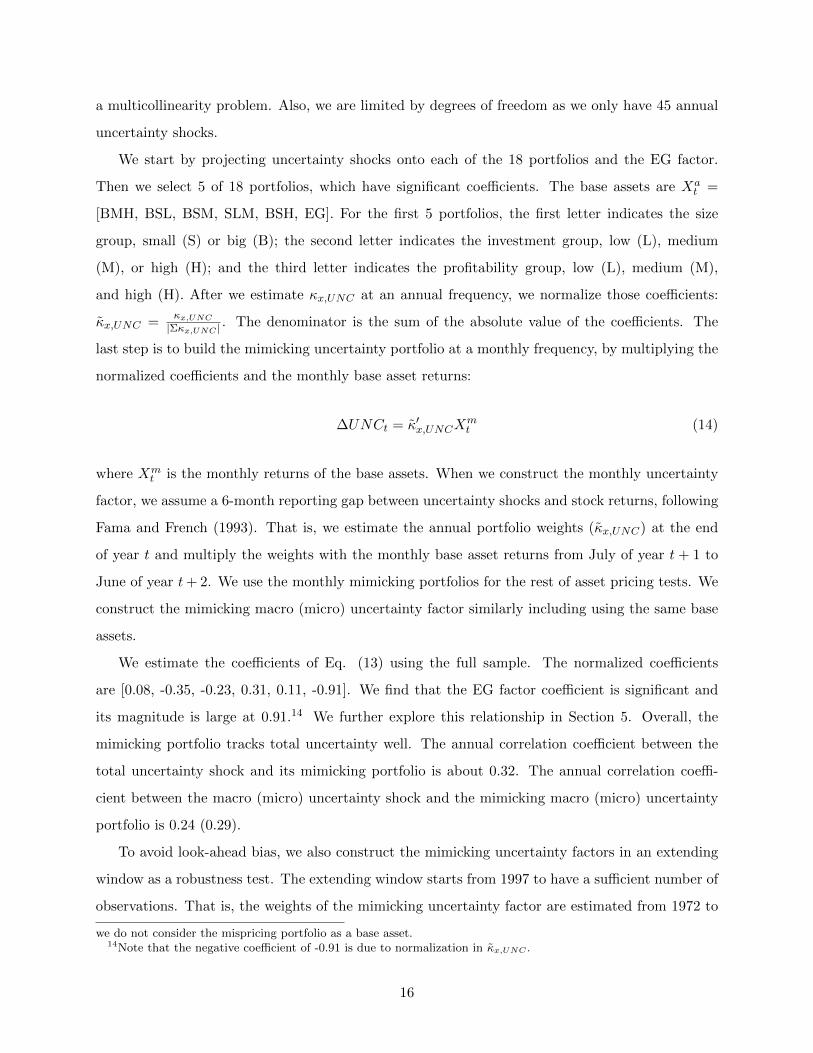
a multicollinearity problem. Also, we are limited by degrees of freedom as we only have 45 annual

uncertainty shocks.

We start by projecting uncertainty shocks onto each of the 18 portfolios and the EG factor.

Then we select 5 of 18 portfolios, which have significant coefficients. The base assets are Xat =

[BMH, BSL, BSM, SLM, BSH, EG]. For the first 5 portfolios, the first letter indicates the size

group, small (S) or big (B); the second letter indicates the investment group, low (L), medium

(M), or high (H); and the third letter indicates the profitability group, low (L), medium (M),

and high (H). After we estimate κx,UNC at an annual frequency, we normalize those coefficients:

κx,UNC =κx,UNC

|Σκx,UNC | . The denominator is the sum of the absolute value of the coefficients. The

last step is to build the mimicking uncertainty portfolio at a monthly frequency, by multiplying the

normalized coefficients and the monthly base asset returns:

∆UNCt = κ′x,UNCXmt (14)

where Xmt is the monthly returns of the base assets. When we construct the monthly uncertainty

factor, we assume a 6-month reporting gap between uncertainty shocks and stock returns, following

Fama and French (1993). That is, we estimate the annual portfolio weights (κx,UNC) at the end

of year t and multiply the weights with the monthly base asset returns from July of year t + 1 to

June of year t+ 2. We use the monthly mimicking portfolios for the rest of asset pricing tests. We

construct the mimicking macro (micro) uncertainty factor similarly including using the same base

assets.

We estimate the coefficients of Eq. (13) using the full sample. The normalized coefficients

are [0.08, -0.35, -0.23, 0.31, 0.11, -0.91]. We find that the EG factor coefficient is significant and

its magnitude is large at 0.91.14 We further explore this relationship in Section 5. Overall, the

mimicking portfolio tracks total uncertainty well. The annual correlation coefficient between the

total uncertainty shock and its mimicking portfolio is about 0.32. The annual correlation coeffi-

cient between the macro (micro) uncertainty shock and the mimicking macro (micro) uncertainty

portfolio is 0.24 (0.29).

To avoid look-ahead bias, we also construct the mimicking uncertainty factors in an extending

window as a robustness test. The extending window starts from 1997 to have a sufficient number of

observations. That is, the weights of the mimicking uncertainty factor are estimated from 1972 to

we do not consider the mispricing portfolio as a base asset.14Note that the negative coefficient of -0.91 is due to normalization in κx,UNC .

16

1997 first, then we extend the estimation period up to 2016. To estimate the weights with enough

degrees of freedom for the extending window, we use 5 base assets: Xat = [SSL, BMM, SLM, BSH,

EG].

4.2. Mimicking uncertainty factors

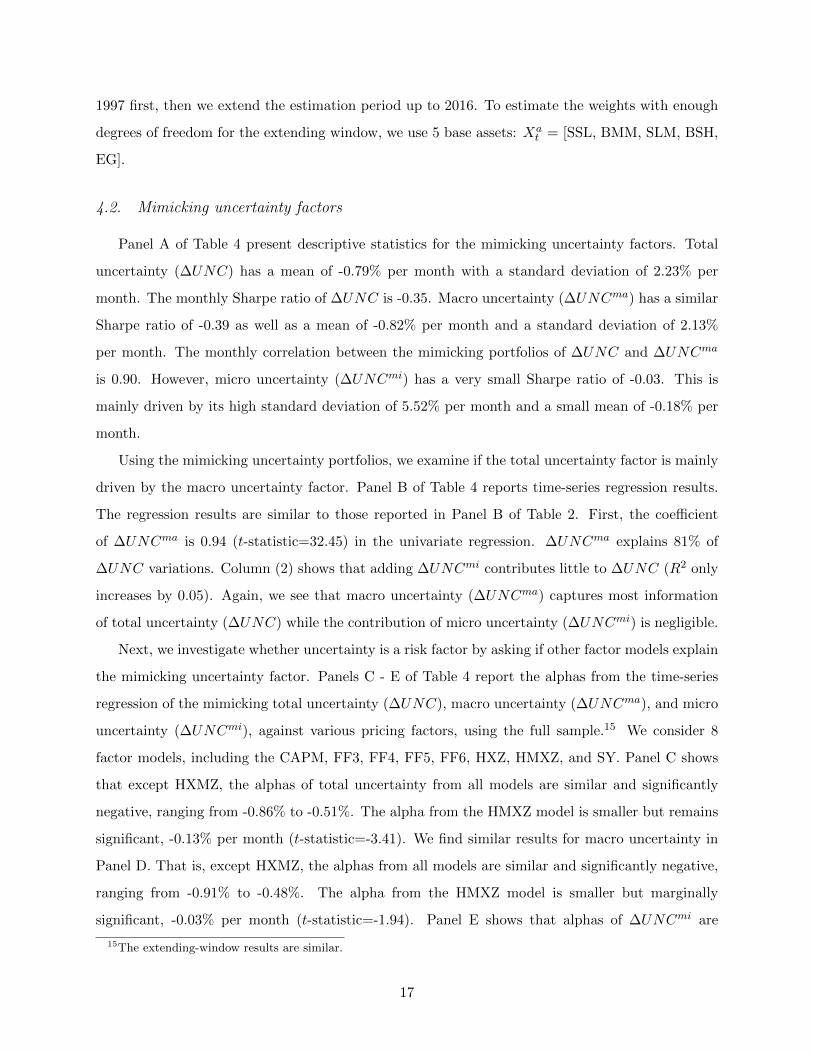
Panel A of Table 4 present descriptive statistics for the mimicking uncertainty factors. Total

uncertainty (∆UNC) has a mean of -0.79% per month with a standard deviation of 2.23% per

month. The monthly Sharpe ratio of ∆UNC is -0.35. Macro uncertainty (∆UNCma) has a similar

Sharpe ratio of -0.39 as well as a mean of -0.82% per month and a standard deviation of 2.13%

per month. The monthly correlation between the mimicking portfolios of ∆UNC and ∆UNCma

is 0.90. However, micro uncertainty (∆UNCmi) has a very small Sharpe ratio of -0.03. This is

mainly driven by its high standard deviation of 5.52% per month and a small mean of -0.18% per

month.

Using the mimicking uncertainty portfolios, we examine if the total uncertainty factor is mainly

driven by the macro uncertainty factor. Panel B of Table 4 reports time-series regression results.

The regression results are similar to those reported in Panel B of Table 2. First, the coefficient

of ∆UNCma is 0.94 (t-statistic=32.45) in the univariate regression. ∆UNCma explains 81% of

∆UNC variations. Column (2) shows that adding ∆UNCmi contributes little to ∆UNC (R2 only

increases by 0.05). Again, we see that macro uncertainty (∆UNCma) captures most information

of total uncertainty (∆UNC) while the contribution of micro uncertainty (∆UNCmi) is negligible.

Next, we investigate whether uncertainty is a risk factor by asking if other factor models explain

the mimicking uncertainty factor. Panels C - E of Table 4 report the alphas from the time-series

regression of the mimicking total uncertainty (∆UNC), macro uncertainty (∆UNCma), and micro

uncertainty (∆UNCmi), against various pricing factors, using the full sample.15 We consider 8

factor models, including the CAPM, FF3, FF4, FF5, FF6, HXZ, HMXZ, and SY. Panel C shows

that except HXMZ, the alphas of total uncertainty from all models are similar and significantly

negative, ranging from -0.86% to -0.51%. The alpha from the HMXZ model is smaller but remains

significant, -0.13% per month (t-statistic=-3.41). We find similar results for macro uncertainty in

Panel D. That is, except HXMZ, the alphas from all models are similar and significantly negative,

ranging from -0.91% to -0.48%. The alpha from the HMXZ model is smaller but marginally

significant, -0.03% per month (t-statistic=-1.94). Panel E shows that alphas of ∆UNCmi are

15The extending-window results are similar.

17

mostly insignificant across different factor models.

Overall, Table 4 demonstrates that macro uncertainty is the main driver of total uncertainty,

which is not fully captured by the existing pricing factors, while the pricing of micro uncertainty

is negligible. Therefore, we will mainly use our macro uncertainty factor (∆UNCma) in the subse-

quent analyses.

4.3. Fama-MacBeth regressions

Our previous results show that macro uncertainty is a significant risk factor that is not explained

by many prevailing factor models while micro uncertainty is captured by many models. Next,

we explore the cross-sectional pricing power of ∆UNCma by running Fama-MacBeth two-pass

regressions.

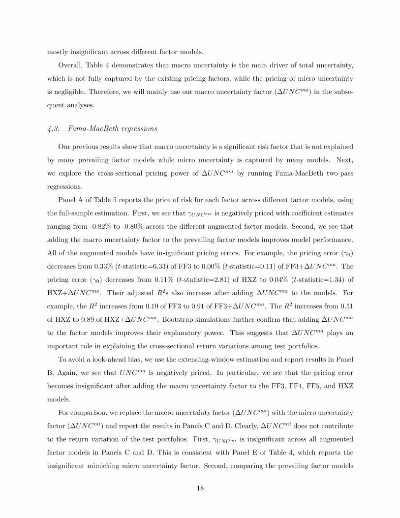
Panel A of Table 5 reports the price of risk for each factor across different factor models, using

the full-sample estimation. First, we see that γUNCma is negatively priced with coefficient estimates

ranging from -0.82% to -0.80% across the different augmented factor models. Second, we see that

adding the macro uncertainty factor to the prevailing factor models improves model performance.

All of the augmented models have insignificant pricing errors. For example, the pricing error (γ0)

decreases from 0.33% (t-statistic=6.33) of FF3 to 0.00% (t-statistic=0.11) of FF3+∆UNCma. The

pricing error (γ0) decreases from 0.11% (t-statistic=2.81) of HXZ to 0.04% (t-statistic=1.34) of

HXZ+∆UNCma. Their adjusted R2s also increase after adding ∆UNCma to the models. For

example, the R2 increases from 0.19 of FF3 to 0.91 of FF3+∆UNCma. The R2 increases from 0.51

of HXZ to 0.89 of HXZ+∆UNCma. Bootstrap simulations further confirm that adding ∆UNCma

to the factor models improves their explanatory power. This suggests that ∆UNCma plays an

important role in explaining the cross-sectional return variations among test portfolios.

To avoid a look-ahead bias, we use the extending-window estimation and report results in Panel

B. Again, we see that UNCma is negatively priced. In particular, we see that the pricing error

becomes insignificant after adding the macro uncertainty factor to the FF3, FF4, FF5, and HXZ

models.

For comparison, we replace the macro uncertainty factor (∆UNCma) with the micro uncertainty

factor (∆UNCmi) and report the results in Panels C and D. Clearly, ∆UNCmi does not contribute

to the return variation of the test portfolios. First, γUNCmi is insignificant across all augmented

factor models in Panels C and D. This is consistent with Panel E of Table 4, which reports the

insignificant mimicking micro uncertainty factor. Second, comparing the prevailing factor models

18

and the ∆UNCmi-augmented models, we see that γ0 does not change much and is still significant.

Third, the adjusted R2 also shows little improvement after adding ∆UNCmi in Panels C and D.

For completeness, we also consider three variations of uncertainty augmented factors models.

First, we directly use the total uncertainty (∆UNC) to augment the prevailing models. We find

qualitative similar results, i.e., ∆UNC is negatively priced and the augmented models explain

various test assets. Second, we consider adding macro and micro uncertainty factors (∆UNCma

and ∆UNCmi) simultaneously to the prevailing models. We find that ∆UNCma is negatively

priced while ∆UNCmi is not priced. Last, we consider using the aggregate uncertainty factor

derived from aggregate TFP data (UNCagg) or the VIX. We construct the mimicking aggregate

uncertainty factor in a way similar to the mimicking macro uncertainty factor. We find that the

aggregate uncertainty factor is negatively priced, but its performance is weaker than the macro

uncertainty factor derived from the cross-section of TFPs estimated from firm-level data. See

Appendix C for more details. Overall, we conclude that adding the uncertainty factor improves

the explanatory power of prevailing factor models and its price of risk is significantly positive in

the cross section. More importantly, this is mainly driven by the macro uncertainty, not the micro

uncertainty.

4.4. Robustness checks: Examining noisy factors

The previous sections shows that the uncertainty factor, in particular the macro uncertainty

factor, explains various test assets. One might wonder whether our cross-sectional results are spu-

riously driven by noisy factors. Here we show that the uncertainty factors cannot have explanatory

power by chance. Similar to Adrian et al. (2014), we randomly draw the uncertainty factor with

replacement. Then, we construct mimicking uncertainty portfolios and rerun the Fama-MacBeth

two-pass regressions. Because we draw factors randomly, the noisy factors should not perform as

well as the original uncertainty augmented factor models. We repeat this simulation 100,000 times

and estimate how likely the noise factors could perform as well as the original model in Table 6.

Specifically, we estimate the probability that the noisy factors generate R2s as large as the original

models (“R2” column), price of uncertainty risk as large as the original models (“PRC” column),

or the Sharpe ratio of an uncertainty factor as large as the original models (“SR” column), or .

We also report the joint probabilities that noisy factors can simultaneously generate higher R2s

and price of risk than the original models (“Joint R2-PRC” column) and that noisy factors can

simultaneously generate higher R2s, larger prices of risk, and Sharpa ratio of uncertainty factor

19

than the original models (“Joint all” column).

In Panel A, we test the noisy total uncertainty (∆UNC) augmented factor models. All noisy

models perform poorly. Taking the noise total uncertainty augmented FF6 model as an example,

the probability of the noisy factors performing as well as the original model is only 4.65%, 0.00%,

and 0.00% in terms of R2, the intercept, and the price of risk, respectively. Moreover, their

joint probabilities are zeros. That is, it is almost impossible for the noisy factors to achieve the

same explanatory power as the original models. In Panel B, we use the macro uncertainty factor

(∆UNCma) and see very similar results. The probability that noisy factors may perform as well

as the original models is less than 7% in terms of R2, while it is 0 for the intercept or the joint

tests. Turning to the micro uncertainty (∆UNCmi) in Panel C, we see the probabilities increase

sharply. This suggests that the noisy factors might perform similarly to the original model for micro

uncertainty. This is not surprising since we find that micro uncertainty factor is not priced. Last,

we perform similar exercises with the non-tradable uncertainty factors directly and find similar

results.16 Overall, the results suggest that the asset pricing power of macro uncertainty is not due

to chance.

5. Interpreting the expected investment growth factor

Tables 1 and 4 show that total uncertainty (macro uncertainty) is highly correlated with the

expected investment growth factor (EG) from Hou et al. (2021). In this section, we further explore

why the EG factor might capture uncertainty risk. This helps us better understand the success of

the EG factor and the q5-model.

We first discuss the economic linkage between the EG factor and uncertainty risk. Then, we

relate the cross-sectional dispersion of EG predictors to the uncertainty factor. Lastly, we compare

the pricing power of the EG factor and the uncertainty factor.

5.1. The expected investment growth factor

Motivated by Eq. (5), Hou et al. (2015) introduce the q-factor model which includes the market

portfolio (MKT), the size factor (QME), the investment factor (QIA), and the profitability factor

(QROE). Hou et al. (2021) further separate the numerator of (5) into the dividend yield, [Xit+1 +

(a/2)(Iit+1/Kit+1)2]/[1+a(Iit/Kit)], and the capital gain, (1−δ)[1+a(Iit+1/Kit+1)]/[1+a(Iit/Kit)],

16These results are available by request.

20

and suggest that the second part captures expected investment growth (EG). They propose the

q5 model by adding the EG factor to the q-factor model and demonstrate its empirical success by

explaining many test portfolios and other pricing factors.

We replicate the EG factor by following Hou et al. (2021). To predict expected future investment

growth, Hou et al. (2021) run Fama-MacBeth regressions, using weighted least squares with market

capitalization, as follows:

d

(IitKit

)= β0 + βQlogQit−1 + βCoPCoPit−1 + βdROEdROEit−1 + εit, (15)

where d(IitKit

)is the first difference of the asset growth of firm i at time t, Q is Tobin’s q, CoP is the

operating cashflow, dROE is the first difference between current ROE and the four-quarter-lagged

ROE. They estimate the regression coefficients using a 120-month rolling window and estimate

the predicted future investment growth as follows:

Et[dIit+1/Kit+1] = β0 + βQlogQit + βCoPCoPit + βdROEdROEit. (16)

After estimating Eq. (16), they sort stocks on size and Et[dIit+1/Kit+1] into 2-by-3 portfo-

lios. They then construct the expected investment growth factor (EG) as the difference between

the average returns of two high Et[dIit+1/Kit+1] portfolios and the average returns of two low

Et[dIit+1/Kit+1] portfolios, following Fama and French (1993). During our sample period, EG fac-

tor has a mean of 0.81% per month, a standard deviation of 2.02%, and an annual Sharpe ratio

of 0.40. Also, untabulated results show that the prevailing factor models cannot explain the EG

factor.

Why is the EG factor highly correlated with the uncertainty factor? First, we see from Eq. (8)

that uncertainty contributes to the expected investment growth. In fact, after controlling for other

pricing factors, the EG factor mainly captures uncertainty risk. Second, the empirical measure of ex-

pected investment growth captures the cross-sectional dispersion of productivity. When predicting

the future investment growth in Eq. (16), the coefficients of the Fama-MacBeth regressions depend

on the cross-sectional variation of each predictor and these cross-sectional variations embed some

productivity dispersions. For example, productivity dispersion clearly affects the cross-sectional

variations of Tobin’s q, operating cash flows, and ROE. Therefore, the EG factor constructed from

running Fama-MacBeth regressions captures productivity dispersions.17 That is, we expect that

17Bachmann and Bayer (2014) show that shocks to productivity dispersion can generate procyclical cross-sectional

21

the productivity dispersion is significantly correlated with the cross-sectional dispersions of the

three predictors in Eq. (15). We formally verify these two reasons.

5.2. Macro uncertainty and expected investment growth

In this subsection, we test whether the pricing power of EG is driven by macro uncertainty

risk, as suggested by Eq. (8). We directly decompose EG into predicted and residual components,

by regressing EG against the macro uncertainty. Following Hou et al. (2021), we match the non-

tradable ∆UNCma to firm-level EG with an at least four-month reporting gap. We regress EG

against ∆UNCma for each firm, using the full sample.18 We sort all stocks into decile portfolios

based on either their predicted EG or residual EG. Portfolio 10 (1) has the highest (lowest) predicted

or residual EG. Then we compute the value-weighted portfolio returns and alphas from various asset

pricing models.

Panel A of Table 7 presents the returns of 10 portfolios sorted by predicted EG. Similar to

Hou et al. (2021), the portfolio returns monotonically increase with predicted EG. The long-short

portfolio (i.e., Portfolio 10 - Portfolio 1) has an average return of 0.89% (t-statistic = 3.59) per

month. Its alpha is also significantly positive from all benchmark models. For example, the long-

short portfolio has an alpha of 0.91% (t-statistic=4.79) and 0.86% (t-statistic = 4.07) from FF6

and HXZ models, respectively. That is, we see that stocks with higher predicted EG have higher

expected returns and the predicted EG is not captured by the existing factors. However, Panel

B shows that the residual EG does not generate significant alphas. Even though the long-short

portfolio return is 0.77% per month (t-statistic=3.63), the alphas from FF6, HXZ, and SY become

insignificant. That is, residual EG does not provide additional information. Therefore, we see that

the pricing power of EG is driven by macro uncertainty risk.

5.3. Macro uncertainty and the predictors of expected investment growth

Next, we further explore which predictors of the expected investment growth capture uncertainty

risk. In each year, we calculate the cross-sectional standard deviation of each predictor in Eq. (15).

Then, we run the time-series regression of the cross-sectional dispersions of predictors against macro

uncertainty (UNCma) in Panel A of Table 8. First, UNCma explains the cross-sectional dispersions

investment rate dispersion. This implies that expected investment growth can be driven by productivity dispersionshocks.

18To avoid the look-ahead bias, we also use the extending-window to decompose EG into predicted and residualcomponents and we have similar findings (See Appendix D and Table D1).

22

of three EG predictors very well. For example, UNCma explains the cross-sectional dispersion of

operating cash flows (DISCOP ) with a coefficient of coefficient of 0.28 (t-statistic=3.21) and an R2

of 0.42. This suggests that UNCma alone well explains the cross-sectional variation of operating

cash flows. Also, UNCma explains the cross-sectional dispersions of Tobin’s Q (DISQ) and changes

in ROE (DISdROE). The R2 for DISQ and DISdROE are 0.25 and 0.38, respectively. In Panel

B of Table 8, we run similar regressions using the micro uncertainty (UNCmi). The regression

results show that UNCmi explains little of the cross-sectional dispersions of the EG predictors, i.e.,

UNCmi is insignificant in all regressions and the highest R2 is 0.11 only.19

Turning to the asset pricing tests, we next explore whether the loadings of the EG factor and the

uncertainty factors are correlated in Table 9. We estimate the loadings of a set of test assets on the

EG factor, the cross-sectional dispersions of its three predictors, the total uncertainty factor, the

macro uncertainty factor, and the micro uncertainty factors. The test assets include 45 portfolios

(used in Table 3) and the tested pricing factors. First, we see that loadings on EG are highly

correlated with those of the total uncertainty factor and the macro uncertainty factor, but not

the micro uncertainty factor, as shown in Columns (1) and (2). Examining loadings on the three

predictors of EG, we see that operating cash flows (COP ) are highly correlated with the total

uncertainty factor and macro uncertainty factor, but Tobin’s q and changes in ROE (DISdROE)

have a small correlation with the uncertainty factors. This is consistent with the finding of Hou

et al. (2021), i.e., operating cash flows is the strongest predictor of future investment growth.20

Therefore, the evidence from factor loadings further strengthens the connection between the EG

factor and the uncertainty factor.

Overall, Tables 8 and 9 suggest that macro uncertainty explains the EG factor via the cross-

sectional dispersions of its predictors, especially the operating cash flow component. Also, micro

uncertainty cannot capture the same fundamental risks of the EG factor because it does not correlate

with the cross-sectional dispersions of the EG predictors.

5.4. Comparing the EG factor and the uncertainty factor: Time-series and cross-sectional

regressions

Here we run time-series regressions to test whether the EG factor and the uncertainty factor

share the same fundamental risks in Table 10. In Panel A of Table 10, we present time-series

19We find similar results for total uncertainty. See Appendix E for more details.20Appendix F further compares the pricing power of these three EG predictors. That is, we augment the Hou et al.

(2015) q-factor model with each predictor of EG. We find that COP is the strongest predictor.

23

regression coefficients of the EG factor against the factor models augmented with the macro un-

certainty factor (∆UNCma). Unconditionally, the EG factor has an average return of 0.81% per

month (t-statistic=8.77). However, the FF3, FF4, FF5, FF6, HXZ, and SY augmented with macro

uncertainty can fully explain the EG factor. For example, the alpha is very close to 0 in these

augmented models. The loading of ∆UNCma is significant and close to -1. 21 When we replace

∆UNCma with ∆UNCmi in Panel B of Table 10, we see that the EG factor has a significant in-

tercept in all regressions. Therefore, it seems that the EG factor captures a large amount of macro

uncertainty risk, which contributes to its pricing power.

We further compare the pricing power of the EG factor and the uncertainty factor in the

cross sectional regressions. We focus on comparing the Hou et al. (2021) q5 model (HMXZ)

with the macro uncertainty-augmented HXZ model (HXZ+∆UNCma) and the micro uncertainty-

augmented HXZ model (HXZ+∆UNCmi). Panels A and C of Table 5 reports the price of risk

and the pricing error of the Fama-MacBeth regressions, using the full-sample estimation. First,

the pricing error (γ0) from HMXZ is 0.07% (t-statistic=2.10) while that of HXZ+∆UNCma is

0.04% (t-statistic=1.34) in Panel A. Again, ∆UNCmi does not play a role in the regressions as

∆UNCmi is insignificant throughout in Panel C. Second, γEG is 0.79% (t-statistic=7.70) in the

HMXZ model while γUNCma is -0.81% (t-statistic=-7.89) in the HXZ+∆UNCma model. That is,

EG and ∆UNCma have a similar price of risk. In Panels B and D of Table 5, we estimate the price

of risk using the extending-window estimation. The main results are qualitatively similar to those in

Panels A and C. The γ0 from HMXZ is 0.06% (t-statistic=0.96) while that from HXZ+∆UNCma

is 0.09% (t-statistic=1.50). Also, γEG and γUNCma are 0.61% (t-statistic=3.32) and -0.68% (t-

statistic=-3.75), while γUNCmi is -1.47% (t-statistic=-0.71).22 Overall, we see that the Hou et al.

(2015) q-factor model augmented with the macro uncertainty factor performs similarly to the Hou

et al. (2021) q5-factor model (HMXZ).

5.5. Comparing various models: Maximum squared Sharpe ratio

In Table 5, we use a set of test assets as the left-hand-side variables to examine the pricing

power of different models. This approach is widely used (see, e.g., Fama and French, 1996, 2015,

2016, 2017; Hou et al., 2015, 2019, 2021). However, this approach is often sensitive to the choice

21Appendix G reports similar regression results, using total uncertainty (∆UNC) to explain the EG factor. Thatis, ∆UNC captures the EG factor in the augmented SY and HXZ models, with insignificant intercepts.

22As a robustness check, we replace macro uncertainty (∆UNCma) with total uncertainty (∆UNC) in AppendixH and find similar results.

24

of test assets. Alternatively, following Barillas and Shanken (2017) and Fama and French (2018),

we use the right-hand-side approach to compare various models. To minimize the max squared

Sharpe ratio of the intercepts for all left-hand-side portfolios, we can rank competing models on

the maximum squared Sharpe ratio for model factors (Barillas and Shanken, 2017).

To test a factor model i with factors fi, consider time-series regressions of the test assets (Πi),

which include non-factor test assets and factors from other competing models, on model i’s factors

fi. Suppose the vector of intercepts from the time-series regressions is ai and the residual covariance

matrix is Σi. The maximum squared Sharpe ratio of the intercepts is

Sh2(ai) = a′iΣ−1i ai, (17)

where Sh2(·) denotes the maximum squared Sharpe ratio. Gibbons et al. (1989) further show

that the maximum squared Sharpe ratio of the intercepts is the difference between the maximum

squared Sharpe ratio constructed by Πi and model i’s factors and that constructed by model i’s

factors only:

Sh2(ai) = Sh2(Πi, fi)− Sh2(fi). (18)

As Πi and fi together include all competing factors, Sh2(Πi, fi) is independent of i. Hence, to

minimize the maximum squared Sharpe ratio of the intercepts, we only need to find the maximum

squared Sharpe ratio for model factors fi, i.e., Sh2(fi). The maximum squared Sharpe ratio can

be computed from the tangent portfolio formed by model factors.

Table 11 presents the maximum squared Sharpe ratios for various factor models. Limited by

data availability, we compare the FF3, FF4, FF5, FF6, HXZ, HMXZ, and macro uncertainty, micro

uncertainty, or total uncertainty augmented models.23 First, we see that adding macro uncertainty

consistently improves the maximum squared Sharpe ratio across all models, suggesting the impor-

tance of macro uncertainty risk. But adding micro uncertainty only significantly improves FF6 and

HXZ models, while adding total uncertainty only significantly improves FF3 model. Second, we

see that HXMZ has the highest maximum squared Sharpe ratio (0.30) while FF6+∆UNCma and

HXZ+∆UNCma have similar maximum squared Sharpe ratio (0.26 and 0.27, respectively). Again,

this suggest that the EG factor and the macro uncertainty factor are very similar.

We close this section by concluding that the expected investment growth factor captures macro

23We cannot compute Sh2(f) for the SY model as we only have the data for the spread factors, not the correspondingportfolios.

25

uncertainty risk. This contributes to the pricing power of the expected investment growth factor

and the success of the q5-model.

6. Conclusions

Both macro and micro uncertainty affect real economic activities. To match business cycle

statistics, the macroeconomic literature often assumes a prominent role for micro uncertainty,

without acknowledging how micro uncertainty might be proxying for macro uncertainty. In this

paper, we use firm-level productivity estimates to decompose total uncertainty into macro and

micro uncertainty. We find that macro uncertainty is strongly countercyclical and priced among a

cross section of stocks, but micro uncertainty is almost acyclical and not priced. During recessions,

both macro uncertainty and the price of macro uncertainty risk increase. Overall, our results from

financial markets cast doubt on the importance of micro uncertainty on the business cycle.

Macro uncertainty appears to be a missing factor in prevailing factor models. Moreover, we

find that macro uncertainty risk drives the pricing power of the expected investment growth factor

proposed in Hou et al. (2021), because uncertainty affects both expected returns and expected

investment growth. Empirically, both uncertainty and the EG predictors, in particular operating

cash flows, capture cross-sectional productivity dispersion. This suggests an alternative way to

understand the success of the EG factor and the q5-model.

26

References

Adrian, T., Etula, E., Muir, T., 2014. Financial intermediaries and the cross-section of asset returns.

Journal of Finance 69, 2557–2596.

Alfaro, I., Bloom, N., Lin, X., 2019. The finance uncertainty multiplier, Working Paper, Stanford

University.

Bachmann, R., Bayer, C., 2013. ‘Wait-and-See’ business cycles? Journal of Monetary Economics

60, 704–719.

Bachmann, R., Bayer, C., 2014. Investment dispersion and the business cycle. American Economic

Review 104, 1392–1416.

Bachmann, R., Elstner, S., Sims, E. R., 2013. Uncertainty and economic activity: Evidence from

business survey data. American Economic Journal: Macroeconomics 5, 217–49.

Bali, T. G., Brown, S. J., Tang, Y., 2017. Is economic uncertainty priced in the cross-section of

stock returns? Journal of Financial Economics 126, 471–489.

Bali, T. G., Subrahmanyam, A., Wen, Q., 2020. The macroeconomic uncertainty premium in the

corporate bond market. Journal of Financial and Quantitative Analysis forthcoming.

Bali, T. G., Zhou, H., 2016. Risk, uncertainty, and expected returns. Journal of Financial and

Quantitative Analysis 51, 707–735.

Bansal, R., Yaron, A., 2004. Risks for the long run: A potential resolution of asset pricing puzzles.

Journal of Finance 59, 1481–1509.

Barillas, F., Shanken, J., 2017. Which alpha? Review of Financial Studies 30, 1316–1338.

Basu, S., Bundick, B., 2017. Uncertainty shocks in a model of effective demand. Econometrica 85,

937–958.

Bekaert, G., Engstrom, E., Xing, Y., 2009. Risk, uncertainty, and asset prices. Journal of Financial

Economics 91, 59–82.

Berger, D., Dew-Becker, I., Giglio, S., 2019. Uncertainty shocks as second-moment news shocks.

Review of Economic Studies 87, 40–76.

Berk, J. B., Green, R. C., Naik, V., 1999. Optimal investment, growth options, and security returns.

Journal of Finance 54, 1553–1607.

Bloom, N., 2009. The impact of uncertainty shocks. Econometrica 77, 623–685.

Bloom, N., 2014. Fluctuations in uncertainty. Journal of Economic Perspectives 28, 153–76.

Bloom, N., Floetotto, M., Jaimovich, N., Saporta-Eksten, I., Terry, S. J., 2018. Really uncertain

27

business cycles. Econometrica 86, 1031–1065.

Carhart, M. M., 1997. On persistence in mutual fund performance. Journal of Finance 52, 57–82.

Chen, H., Chen, S., 2012. Investment-cash flow sensitivity cannot be a good measure of financial

constraints: Evidence from the time series. Journal of Financial Economics 103, 393–410.

Chen, Z., 2016. Time-to-produce, inventory, and asset prices. Journal of Financial Economics 120,

330–345.

Chen, Z., Connor, G., Korajczyk, R. A., 2018. A performance comparison of large-n factor estima-

tors. Review of Asset Pricing Studies 8, 153–182.

Chen, Z., Kim, B.-C., 2019. Fundamental risk sources and pricing factors, Working Paper, Hong

Kong University of Science and Technology.

Chen, Z., Petkova, R., 2012. Does idiosyncratic volatility proxy for risk exposure? Review of

Financial Studies 25, 2745–2787.

Chen, Z., Yang, B., 2019. In search of preference shock risks: Evidence from longevity risks and

momentum profits. Journal of Financial Economics 133, 225–249.

Cochrane, J. H., 1991. Production-based asset pricing and the link between stock returns and

economic fluctuation. Journal of Finance 46, 209–237.

Cochrane, J. H., 1996. A cross-sectional test of an investment-based asset pricing model. Journal

of Political Economy 104, 572–621.

Connor, G., Korajczyk, R. A., 1987. Estimating pervasive economic factors with missing observa-

tions, Working Paper, http://ssrn.com/abstract=1268954.

David, J., Schmid, L., Zeke, D., 2018. Risk-adjusted capital allocation and misallocation, Working

Paper, Duke University.

Dew-Becker, I., Giglio, S., 2020. Cross-sectional uncertainty and the business cycle: Evidence from

40 years of options data, Working Paper, Northwestern University.

Dew-Becker, I., Giglio, S., Kelly, B. T., 2019. Hedging macroeconomic and financial uncertainty

and volatility, NBER Working Paper No. 26323.

Dew-Becker, I., Giglio, S., Le, A., Rodriguez, M., 2017. The price of variance risk. Journal of

Financial Economics 123, 225–250.

Fama, E. F., French, K. R., 1993. Common risk factors in the returns on stocks and bonds. Journal

of Financial Economics 33, 3–56.

Fama, E. F., French, K. R., 1996. Multifactor explanations of asset pricing anomalies. Journal of

Finance 51, 55–84.

28

Fama, E. F., French, K. R., 2015. A five-factor asset pricing model. Journal of Financial Economics

116, 1–22.

Fama, E. F., French, K. R., 2016. Dissecting anomalies with a five-factor model. Review of Financial

Studies 29, 69–103.

Fama, E. F., French, K. R., 2017. International tests of a five-factor asset pricing model. Journal

of Financial Economics 123, 441–463.

Fama, E. F., French, K. R., 2018. Choosing factors. Journal of Financial Economics 128, 234–252.

Fernandez-Villaverde, J., Guerron-Quintana, P., Kuester, K., Rubio-Ramırez, J., 2015. Fiscal

volatility shocks and economic activity. American Economic Review 105, 3352–84.

Fernandez-Villaverde, J., Guerron-Quintana, P. A., 2020. Uncertainty shocks and business cycle

research, NBER Working Paper No. 26768.

Foster, L., Haltiwanger, J. C., Krizan, C. J., 2001. Aggregate productivity growth: Lessons from

microeconomic evidence. In: New developments in productivity analysis, University of Chicago

Press, pp. 303–372.

Gibbons, M. R., Ross, S. A., Shanken, J., 1989. A test of the efficiency of a given portfolio.

Econometrica 57, 1121–1152.

Hartzmark, S. M., 2016. Economic uncertainty and interest rates. Review of Asset Pricing Studies

6, 179–220.

Herskovic, B., Kelly, B., Lustig, H., Nieuwerburgh, S. V., 2016. The common factor in idiosyncratic

volatility: Quantitative asset pricing implications. Journal of Financial Economics 119, 249–283.

Herskovic, B., Kind, T., Kung, H., 2020. Micro uncertainty and asset prices, Working Paper,

London Business School.

Hou, K., Mo, H., Xue, C., Zhang, L., 2019. Which factors? Review of Finance 23, 1–35.

Hou, K., Mo, H., Xue, C., Zhang, L., 2021. An augmented q-factor model with expected growth.

Review of Finance 25, 1–41.

Hou, K., Xue, C., Zhang, L., 2015. Digesting anomalies: An investment approach. Review of

Financial Studies 28, 650–705.

Imrohoroglu, A., Tuzel, Selale., 2014. Firm-level productivity, risk, and return. Management Science

60, 1861–2109.

Jagannathan, R., Wang, Z., 1996. The conditional CAPM and the cross-section of expected returns.

Journal of Finance 51, 3–53.

Jurado, K., Ludvigson, S. C., Ng, S., 2015. Measuring uncertainty. American Economic Review

29

105, 1177–1216.

Kehrig, M., 2015. The cyclical nature of the productivity distribution, Working Paper, Duke Uni-

versity.

Kozeniauskas, N., Orlik, A., Veldkamp, L., 2018. What are uncertainty shocks? Journal of Monetary

Economics 100, 1–15.

Lettau, M., Ludvigson, S., 2002. Time-varying risk premia and the cost of capital: An alternative

implication of the Q theory of investment. Journal of Monetary Economics 49, 31–66.

Lewellen, J., Nagel, S., Shanken, J., 2010. A skeptical appraisal of asset-pricing tests. Journal of

Financial Economics 96, 175–194.

Li, J., Wang, H., Yu, J., 2020. Aggregate expected investment growth and stock market returns.

Journal of Monetary Economics forthcoming.

Liu, L. X., Whited, T. M., Zhang, L., 2009. Investment-based expected stock returns. Journal of

Political Economy 117, 1105–1139.

Olley, G. S., Pakes, A., 1996. The dynamics of productivity in the telecommunications equipment

industry. Econometrica 64, 1263–1297.

Restoy, F., Rockinger, G. M., 1994. On stock market returns and returns on investment. Journal

of Finance 49, 543–556.

Schaab, A., 2020. Micro and macro uncertainty, Working Paper, Harvard University.

Segal, G., Shaliastovich, I., Yaron, A., 2015. Good and bad uncertainty: Macroeconomic and

financial market implications. Journal of Financial Economics 117, 369 – 397.

Shanken, J., 1992. On the estimation of beta-pricing models. Review of Financial Studies 5, 1–55.

Stambaugh, R. F., Yuan, Y., 2017. Mispricing factors. Review of Financial Studies 30, 1270–1315.

Zhang, L., 2005. The value premium. Journal of Finance 60, 67–103.

30

1975 1980 1985 1990 1995 2000 2005 2010 2015

Year

-3

-2

-1

0

1

2

3

UNC UNCma UNCmi IP

Fig. 1. Uncertainty and industrial production growth

This figure plots the time series of total uncertainty (UNC), macro uncertainty (UNCma), andmicro uncertainty (UNCmi) against the annual log industrial production (IP) growth in the UnitedStates. Series are computed from Christiano and Fitzgerald (2003) band-pass filter and standard-ized. The shaded areas are NBER recession periods.

31

1975 1980 1985 1990 1995 2000 2005 2010 2015

Year

-3

-2

-1

0

1

2

3

4

UNC RD RDsys RDidio

(a) Total uncertainty and return dispersions

1975 1980 1985 1990 1995 2000 2005 2010 2015

Year

-3

-2

-1

0

1

2

3

4

UNCma RD RDsys RDidio

(b) Macro uncertainty and return dispersions

1975 1980 1985 1990 1995 2000 2005 2010 2015

Year

-3

-2

-1

0

1

2

3

4

UNCmi RD RDsys RDidio

(c) Micro uncertainty and return dispersions

Fig. 2. Uncertainty and stock return dispersions

These figures plot the time series of total uncertainty (UNC), macro uncertainty (UNCma), andmicro uncertainty (UNCmi) against cross-sectional return dispersions, including total stock returndispersion (RD), the systematic stock return dispersion (RDsys) and the idiosyncratic return dis-persion (RDidio) computed from the Carhart four-factor model. All series are standardized. Theshaded areas are NBER recession periods.

32

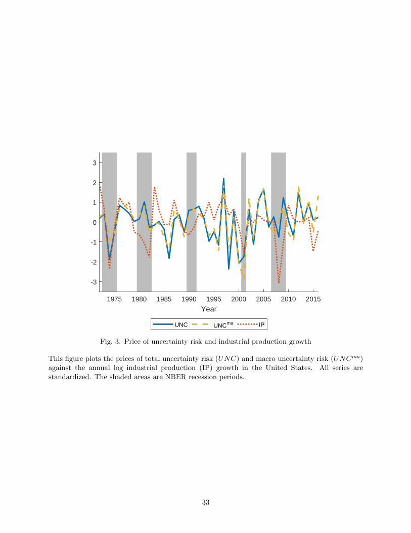
1975 1980 1985 1990 1995 2000 2005 2010 2015

Year

-3

-2

-1

0

1

2

3

UNC UNCma IP

Fig. 3. Price of uncertainty risk and industrial production growth

This figure plots the prices of total uncertainty risk (UNC) and macro uncertainty risk (UNCma)against the annual log industrial production (IP) growth in the United States. All series arestandardized. The shaded areas are NBER recession periods.

33

Tab

le1.

Uncertainty

facto

rs:Descriptivestatisticsand

relationswith

oth

erpricingfacto

rs

Panel

Asu

mm

ari

zes

the

annual

TF

Pgro

wth

(∆T

FP

),th

efirs

t-diff

eren

ceof

cross

-sec

tional

standard

dev

iati

on

of

TF

Pgro

wth

(tota

lunce

rtain

ty,

∆UNC

),sy

stem

ati

cT

FP

gro

wth

(macr

ounce

rtain

ty,

∆UNC

ma),

and

idio

syncr

ati

cT

FP

gro

wth

(mic

rounce

rtain

ty,

∆UNC

mi),

incl

udin

gth

em

ean,

standard

dev

iati

on,

per

centi

les,

corr

elati

on

wit

hin

dust

rial

pro

duct

ion

(IP

)gro

wth

(ρ(IP

))and

annual

changes

inV

IX(ρ

(∆VIX

)).

We

regre

ssfirm

-lev

elT

FP

gro

wth

on

six

pri

nci

pal

com

ponen

tsof

TF

Pfo

rea

chfirm

and

defi

ne

pre

dic

ted

(res

idual)

TF

Pgro

wth

as

syst

emati

c(i

dio

syncr

ati

c)T

FP

gro

wth

.P

anel

Bre

port

sth

eannual

tim

e-se

ries

corr

elati

on

coeffi

cien

tsb

etw

een

vari

ous

unce

rtain

tym

easu

res

and

pri

cing

fact

ors

.T

he

sam

ple

of

unce

rtain

tyes

tim

ate

sis

from

1972

to2016.

Panel

A:

TF

Pand

its

unce

rtain

tym

easu

res

Mea

nS.D

.M

inM

ax

10%

25%

50%

75%

90%

AR

(1)

ρ(IP

)ρ(∆VIX

)∆

TF

P0.0

10.2

1-0

.71

2.0

3-0

.21

-0.1

0-0

.01

0.0

90.2

2-0

.08

∆UNC

0.0

00.0

5-0

.15

0.1

4-0

.05

-0.0

10.0

10.0

20.0

4-0

.53

-0.1

00.3

8∆UNC

ma

0.0

00.0

7-0

.23

0.1

9-0

.07

-0.0

20.0

10.0

30.0

7-0

.60

-0.2

60.3

7∆UNC

mi

0.0

00.0

3-0

.05

0.0

7-0

.04

-0.0

10.0

00.0

20.0

4-0

.66

0.0

0-0

.18

Panel

B:

Corr

elati

ons

bet

wee

nT

FP

unce

rtain

tyand

pri

cing

fact

ors

MK

TSM

BH

ML

CM

AR

MW

UM

DQ

ME

QIA

QROE

EG

MIS

∆UNC

∆UNC

ma

MK

T1.0

0SM

B0.1

01.0

0H

ML

-0.3

20.0

51.0

0C

MA

-0.3

20.2

20.6

51.0

0R

MW

-0.2

6-0

.06

0.4

00.2

41.0

0U

MD

0.1

90.1

9-0

.25

-0.1

1-0

.05

1.0

0Q

ME

0.1

50.9

80.0

50.2

1-0

.13

0.2

61.0

0Q

IA

-0.2

70.1

90.6

30.9

10.2

8-0

.10

0.1

81.0

0Q

ROE

0.0

10.0

10.0

90.0

00.5

40.4

80.0

50.1

71.0

0E

G-0

.15

0.1

70.1

10.2

60.3

50.3

20.1

60.2

80.4

51.0

0M

IS-0

.26

-0.0

20.0

20.3

50.4

10.4

5-0

.03

0.3

40.4

50.6

81.0

0∆UNC

0.0

4-0

.19

-0.0

50.0

00.2

3-0

.18

-0.2

40.0

60.1

50.2

90.1

11.0

0∆UNC

ma

-0.0

1-0

.18

-0.0

8-0

.02

0.1

4-0

.15

-0.2

30.0

00.0

40.2

50.0

70.8

71.0

0∆UNC

mi

0.1

50.0

00.0

30.0

2-0

.06

0.1

50.0

3-0

.01

0.0

9-0

.15

-0.0

3-0

.36

-0.6

3

34

Table 2. Decomposing total uncertainty into macro and micro uncertainty

Panel A presents the time-series regression of the aggregate uncertainty on macro uncertainty (UNCma) and microuncertainty (UNCmi). The aggregate uncertainty (UNCagg) is the conditional standard deviation of a generalizedautoregressive conditional heteroskedasticity GARCH(1,1) on aggregate TFP, obtained from Federal Reserve SanFrancisco. Panel B presents the time-series regression of total uncertainty (∆UNC) on macro uncertainty (UNCma)and micro uncertainty (UNCmi). Newey-West adjusted t-statistics with 5-year lags are in parentheses. The testingperiod is from 1972 to 2016.

Panel A: Regression of aggregate uncertainty against macro and micro uncertainty

(1) (2)UNCagg UNCagg

UNCma 0.25 0.24(2.23) (2.21)

UNCmi -0.17(-1.25)

R2 0.10 0.11

Panel B: Regression of total uncertainty against macro and micro uncertainty

(1) (2)∆UNC ∆UNC

∆UNCma 0.60 0.73(10.11) (9.62)

∆UNCma 0.53(3.11)

R2 0.75 0.81

35

Tab

le3.

Cro

ss-sectionalre

gre

ssionsofuncertainty

facto

raugmented

models

This

table

rep

ort

sF

am

a-M

acB

eth

regre

ssio

ns

of

vari

ous

fact

or

model

sand

those

augm

ente

dw

ith

the

unce

rtain

tyfa

ctor,

usi

ng

annual

non-t

radable

unce

rtain

tyfa

ctors

dir

ectl

yand

full-s

am

ple

esti

mati

on.

Panel

Ause

sto

tal

unce

rtain

tyfa

ctor

(∆UNC

);P

anel

Buse

sm

acr

ounce

rtain

tyfa

ctor

(∆UNC

ma);

Panel

Cuse

sm

icro

unce

rtain

tyfa

ctor

(∆UNC

mi).

Tes

tass

ets

are

45

port

folios

and

the

test

edpri

cing

fact

ors

,in

cludin

g6

size

and

book-t

o-m

ark

etso

rted

port

folios,

6si

zeand

op

erati

ng

pro

fita

bilit

yso

rted

port

folios,

6si

zeand

inves

tmen

tso

rted

port

folios,

6si

zeand

mom

entu

mso

rted

port

folios,

6si

zeand

exp

ecte

din

ves

tmen

tgro

wth

sort

edp

ort

folios,

10

op

erati

ng

acc

rual

sort

edp

ort

folios,

and

5F

am

a-F

rench

indust

ryp

ort

folios.

Tes

ted

fact

or

model

sare

Fam

aand

Fre

nch

(1993)

thre

e-fa

ctor

model

(FF

3),

Carh

art

(1997)

four-

fact

or

model

(FF

4),

Fam

aand

Fre

nch

(2015)

five-

fact

or

model

(FF

5),

Fam

aand

Fre

nch

(2018)

six-f

act

or

model

(FF

6),

Hou

etal.

(2015)q-

fact

or

model

(HX

Z),

and

Hou

etal.

(2021)q5

model

(HM

XZ

).A

llco

effici

ents

are

mult

iplied

by

100.

Thet-

stati

stic

sare

adju

sted

for

erro

rs-i

n-v

ari

able

s,fo

llow

ing

Shanken

(1992).

The

adju

stedR

2fo

llow

sJagannath

an

and

Wang

(1996).

The

5th

and

95th

per

centi

les

of

the

adju

stedR

2dis

trib

uti

on

from

ab

oots

trap

sim

ula

tion

of

10,0

00

tim

esare

rep

ort

edin

bra

cket

s.T

he

test

ing

per

iod

isJuly

1973

toJune

2018.

Panel

A:

Fact

or

model

saugm

ente

dw

ith

tota

lunce

rtain

ty

FF

3F

F3+

∆UNC

FF

4F

F4+

∆UNC

FF

5F

F5+

∆UNC

FF

6F

F6+

∆UNC

Coeff

t-st

at

Coeff

t-st

at

Coeff

t-st

at

Coeff

t-st

at

Coeff

t-st

at

Coeff

t-st

at

Coeff

t-st

at

Coeff

t-st

at

γ0

2.4

56.4

51.9

62.7

21.3

14.0

71.0

21.7

20.8

92.5

50.8

32.0

20.6

92.3

30.6

61.5

2γM

KT

4.8

61.8

74.9

81.8

86.1

42.3

76.0

32.3

05.9

72.3

05.9

72.3

06.3

52.4

56.3

22.4

2γSM

B2.1

11.1

32.2

51.1

92.1

91.1

72.3

51.2

42.2

51.2

12.3

11.2

32.2

31.2

02.3

41.2

4γH

ML

3.4

11.5

22.5

61.0

14.2

51.8

43.2

31.2

21.9

30.8

81.8

50.8

43.0

01.3

82.9

71.3

3γCM

A5.2

33.9

34.9

63.6

85.2

33.8

84.7

03.2

9γRM

W2.9

41.8

03.3

01.9

72.3

91.4

52.9

61.6

3γUM

D9.8

64.3

59.5

64.1

69.8

24.3

49.7

04.2

7γUN

C-8

.35

-2.8

1-9

.32

-2.7

0-4

.55

-2.0

5-7

.41

-2.5

9R

20.2

10.3

70.5

40.7

60.4

50.4

60.7

10.7

8

(5th

,95th

)(0

.01,

0.5

9)

(0.0

4,

0.6

7)

(0.2

9,

0.7

6)

(0.3

9,

0.8

1)

(0.1

7,

0.7

6)

(0.2

0,

0.7

8)

(0.4

7,

0.8

4)

(0.5

2,

0.8

6)

HX

ZH

XZ

+∆UNC

HM

XZ

Coeff

t-st

at

Coeff

t-st

at

Coeff

t-st

at

γ0

1.7

13.3

21.5

62.0

01.5

22.1

7γM

KT

5.5

72.1

35.4

82.0

35.3

31.6

8γQ

ME

2.6

21.3

62.1

81.0

92.4

31.2

4γQ

IA

3.7

22.2

03.6

51.6

44.6

02.3

4γQ

RO

E5.2

83.2

95.8

93.1

45.4

32.9

9γEG

11.8

97.3

0γUN

C-7

.12

-2.5

7R

20.4

50.5

30.9

1

(5th

,95th

)(0

.11,

0.7

7)

(0.1

6,

0.8

0)

(0.6

3,

0.9

0)

36

Pan

elB

:F

acto

rm

od

els

augm

ente

dw

ith

mac

rou

nce

rtai

nty

FF

3+∆UNCma

FF

4+∆UNCma

FF

5+∆UNCma

FF

6+∆UNCma

HX

Z+

∆UNCma

Coeff

t-st

atC

oeff

t-st

atC

oeff

t-st

atC

oeff

t-st

atC

oeff

t-st

at

γ0

1.61

2.16

0.95

1.80

0.71

1.64

0.58

1.54

1.6

11.9

5γMKT

5.43

2.04

6.25

2.39

6.17

2.37

6.50

2.50

5.5

22.0

4γSMB

2.38

1.26

2.42

1.28

2.36

1.26

2.35

1.26

γHML

2.52

0.96

3.29

1.29

2.02

0.90

3.09

1.40

γCMA

4.97

3.63

4.91

3.54

γRMW

3.50

2.09

2.99

1.77

γUMD

9.45

4.12

9.67

4.27

γQ

ME

2.1

91.0

9γQ

IA

3.1

31.3

4γQ

ROE

5.8

63.0

1γUNC

ma

-13.

93-2

.79

-12.

38-2

.64

-8.2

9-2

.52

-8.7

6-2

.46

-11.2

3-2

.72

R2

0.42

0.71

0.47

0.74

0.5

4(5th

,95th

)(0

.05,

0.68

)(0

.36,

0.80

)(0

.20,

0.78

)(0

.49,

0.85

)(0

.15,

0.7

9)

Pan

elC

:F

acto

rm

od

els

augm

ente

dw

ith

mic

rou

nce

rtai

nty

FF

3+∆UNCmi

FF

4+∆UNCmi

FF

5+∆UNCmi

FF

6+∆UNCmi

HX

Z+

∆UNCmi

Coeff

t-st

atC

oeff

t-st

atC

oeff

t-st

atC

oeff

t-st

atC

oeff

t-st

at

γ0

2.52

5.83

1.34

3.94

0.86

2.40

0.64

1.96

1.7

33.2

5γMKT

4.88

1.88

6.14

2.37

5.93

2.29

6.26

2.42

5.5

72.1

3γSMB

2.14

1.15

2.20

1.18

2.22

1.19

2.18

1.17

γHML

3.24

1.42

4.18

1.81

1.99

0.90

3.14

1.44

γCMA

5.34

4.03

5.43

4.02

γRMW

2.81

1.73

2.11

1.28

γUMD

9.83

4.33

9.88

4.36

γQ

ME

2.6

21.3

6γQ

IA

3.6

52.1

3γQ

ROE

5.3

13.3

5γUNC

mi

1.31

1.46

0.44

0.45

-0.5

1-0

.55

-1.2

4-1

.21

0.2

90.3

2R

20.

200.

530.

440.

710.4

4(5th

,95th

)(0

.03,

0.63

)(0

.30,

0.77

)(0

.21,

0.77

)(0

.48,

0.85

)(0

.14,

0.7

8)

37

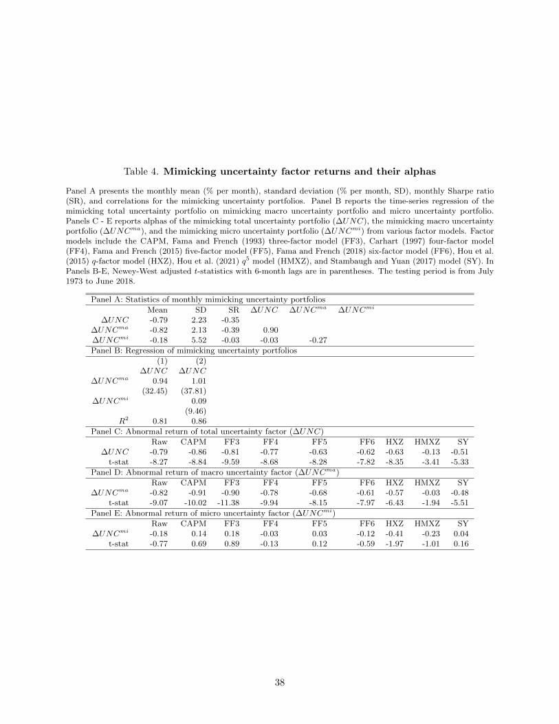
Table 4. Mimicking uncertainty factor returns and their alphas

Panel A presents the monthly mean (% per month), standard deviation (% per month, SD), monthly Sharpe ratio(SR), and correlations for the mimicking uncertainty portfolios. Panel B reports the time-series regression of themimicking total uncertainty portfolio on mimicking macro uncertainty portfolio and micro uncertainty portfolio.Panels C - E reports alphas of the mimicking total uncertainty portfolio (∆UNC), the mimicking macro uncertaintyportfolio (∆UNCma), and the mimicking micro uncertainty portfolio (∆UNCmi) from various factor models. Factormodels include the CAPM, Fama and French (1993) three-factor model (FF3), Carhart (1997) four-factor model(FF4), Fama and French (2015) five-factor model (FF5), Fama and French (2018) six-factor model (FF6), Hou et al.(2015) q-factor model (HXZ), Hou et al. (2021) q5 model (HMXZ), and Stambaugh and Yuan (2017) model (SY). InPanels B-E, Newey-West adjusted t-statistics with 6-month lags are in parentheses. The testing period is from July1973 to June 2018.

Panel A: Statistics of monthly mimicking uncertainty portfolios

Mean SD SR ∆UNC ∆UNCma ∆UNCmi

∆UNC -0.79 2.23 -0.35∆UNCma -0.82 2.13 -0.39 0.90∆UNCmi -0.18 5.52 -0.03 -0.03 -0.27

Panel B: Regression of mimicking uncertainty portfolios

(1) (2)∆UNC ∆UNC

∆UNCma 0.94 1.01(32.45) (37.81)

∆UNCmi 0.09(9.46)

R2 0.81 0.86

Panel C: Abnormal return of total uncertainty factor (∆UNC)

Raw CAPM FF3 FF4 FF5 FF6 HXZ HMXZ SY∆UNC -0.79 -0.86 -0.81 -0.77 -0.63 -0.62 -0.63 -0.13 -0.51

t-stat -8.27 -8.84 -9.59 -8.68 -8.28 -7.82 -8.35 -3.41 -5.33

Panel D: Abnormal return of macro uncertainty factor (∆UNCma)

Raw CAPM FF3 FF4 FF5 FF6 HXZ HMXZ SY∆UNCma -0.82 -0.91 -0.90 -0.78 -0.68 -0.61 -0.57 -0.03 -0.48

t-stat -9.07 -10.02 -11.38 -9.94 -8.15 -7.97 -6.43 -1.94 -5.51

Panel E: Abnormal return of micro uncertainty factor (∆UNCmi)

Raw CAPM FF3 FF4 FF5 FF6 HXZ HMXZ SY∆UNCmi -0.18 0.14 0.18 -0.03 0.03 -0.12 -0.41 -0.23 0.04

t-stat -0.77 0.69 0.89 -0.13 0.12 -0.59 -1.97 -1.01 0.16

38

Tab

le5.

Cro

ss-sectionalre

gre

ssionsofmim

ickinguncertainty

facto

rsaugmented

models

Panel

Are

port

sF

am

a-M

acB

eth

regre

ssio

ns

of

vari

ous

fact

or

model

sand

those

augm

ente

dw

ith

the

month

lym

imic

kin

gm

acr

ounce

rtain

tyfa

ctor

(∆UNC

ma),

usi

ng

the

full-s

am

ple

esti

mati

on.

Panel

Bsh

ows

sim

ilar

resu

lts

wit

hth

eex

tendin

g-w

indow

esti

mati

on.

Panel

Cpre

sents

Fam

a-M

acB

eth

regre

ssio

ns

of

mim

ickin

gm

icro

unce

rtain

ty(∆UNC

mi)

augm

ente

dfa

ctor

model

s.P

anel

Dsh

ows

sim

ilar

resu

lts

wit

hth

eex

tendin

gw

indow

esti

mati

on.

Tes

tass

ets

are

45

port

folios

and

the

test

edpri

cing

fact

ors

,in

cludin

g6

size

and

book-t

o-m

ark

etso

rted

port

folios,

6si

zeand

op

erati

ng

pro

fita

bilit

yso

rted

port

folios,

6si

zeand

inves

tmen

tso

rted

port

folios,

6si

zeand

mom

entu

mso

rted

port

folios,

6si

zeand

exp

ecte

din

ves

tmen

tgro

wth

sort

edp

ort

folios,

10

op

erati

ng

acc

rual

sort

edp

ort

folios,

and

5F

am

a-F

rench

indust

ryp

ort

folios.

Tes

ted

fact

or

model

sare

Fam

aand

Fre

nch

(1993)

thre

e-fa

ctor

model

(FF

3),

Carh

art

(1997)

four-

fact

or

model

(FF

4),

Fam

aand

Fre

nch

(2015)

five-

fact

or

model

(FF

5),

Fam

aand

Fre

nch

(2018)

six-f

act

or

model

(FF

6),

Hou

etal.

(2015)q-

fact

or

model

(HM

Z),

and

Sta

mbaugh

and

Yuan

(2017)

model

(SY

).A

llco

effici

ents

are

mult

iplied

by

100.

Thet-

stati

stic

sare

adju

sted

for

erro

rs-i

n-v

ari

able

s,fo

llow

ing

Shanken

(1992).

The

adju

sted

R2

follow

sJagannath

an

and

Wang

(1996).

The

5th

and

95th

per

centi

les

of

the

adju

stedR

2dis

trib

uti

on

from

ab

oots

trap

sim

ula

tion

of

10,0

00

tim

esare

rep

ort

edin

bra

cket

s.T

he

test

ing

per

iod

for

Panel

Aand

Cis

from

July

1973

toJune

2018

(July

1997

toJune

2018).

The

test

ing

per

iod

for

Panel

Band

Dis

from

July

1997

toJune

2018.

Panel

A:

Fact

or

model

saugm

ente

dw

ith

macr

ounce

rtain

ty,

usi

ng

the

full-s

am

ple

esti

mati

on

FF

3F

F3+

∆UNC

ma

FF

4F

F4+

∆UNC

ma

FF

5F

F5+

∆UNC

ma

FF

6F

F6+

∆UNC

ma

Coeff

t-st

at

Coeff

t-st

at

Coeff

t-st

at

Coeff

t-st

at

Coeff

t-st

at

Coeff

t-st

at

Coeff

t-st

at

Coeff

t-st

at

γ0

0.3

36.3

30.0

00.1

10.0

83.6

10.0

10.4

90.0

93.5

50.0

20.9

20.0

62.8

00.0

31.3

6γM

KT

0.2

91.4

60.5

92.9

70.5

62.8

70.5

92.9

90.5

02.5

50.5

82.9

30.5

62.8

60.5

72.9

3γSM

B0.1

91.4

70.2

92.1

90.2

31.7

40.2

92.1

90.2

72.1

00.2

82.1

70.2

72.0

90.2

82.1

7γH

ML

0.2

11.5

70.2

92.1

20.3

62.6

70.2

92.1

30.1

30.9

50.3

02.2

60.2

51.8

80.3

02.2

7γCM

A0.3

94.0

90.2

82.9

60.3

03.2

90.2

72.9

7γRM

W0.2

01.8

40.2

32.2

00.1

81.7

00.2

32.2

0γUM

D0.6

23.2

90.5

83.0

50.6

03.1

90.5

73.0

2γUN

Cm

a-0

.80

-7.0

0-0

.80

-7.8

4-0

.82

-7.5

3-0

.82

-8.5

8R

20.1

90.9

10.5

10.9

10.5

10.9

10.6

40.9

1

(5th

,95th

)(0

.02,

0.5

0)

(0.8

0,

0.9

2)

(0.3

3,

0.7

0)

(0.8

1,

0.9

3)

(0.2

9,

0.7

2)

(0.8

1,

0.9

3)

(0.4

6,

0.8

0)

(0.8

3,

0.9

3)

Panel

A(C

onti

nued

)

HX

ZH

XZ

+∆UNC

ma

HM

XZ

SY

SY

+∆UNC

ma

Coeff

t-st

at

Coeff

t-st

at

Coeff

t-st

at

Coeff

t-st

at

Coeff

t-st

at

γ0

0.1

12.8

10.0

41.3

40.0

72.1

00.0

81.6

00.0

61.4

6γM

KT

0.5

02.5

00.5

62.8

40.5

42.7

20.5

12.4

80.5

22.5

4γQ

ME

0.3

52.5

50.3

62.6

30.3

62.6

2γQ

IA

0.2

92.7

10.3

63.4

40.3

12.9

3γQ

RO

E0.4

53.3

20.3

62.6

60.3

32.4

0γEG

0.7

97.7

0γM

ISM

E0.4

03.0

60.4

73.6

3γM

GM

T0.5

33.5

70.4

53.0

0γPERF

0.5

52.9

30.5

32.8

2γUN

Cm

a-0

.81

-7.8

9-0

.80

-8.1

0R

20.5

10.8

90.8

20.7

00.9

0

(5th

,95th

)(0

.30,

0.7

1)

(0.7

9,

0.9

2)

(0.6

6,

0.8

7)

(0.5

1,

0.8

2)

(0.7

9,

0.9

2)

39

Panel

B:

Fact

or

model

saugm

ente

dw

ith

macr

ounce

rtain

ty,

usi

ng

the

exte

ndin

g-w

indow

esti

mati

on

FF

3F

F3+

∆UNC

ma

FF

4F

F4+

∆UNC

ma

FF

5F

F5+

∆UNC

ma

FF

6F

F6+

∆UNC

ma

Coeff

t-st

at

Coeff

t-st

at

Coeff

t-st

at

Coeff

t-st

at

Coeff

t-st

at

Coeff

t-st

at

Coeff

t-st

at

Coeff

t-st

at

γ0

0.2

22.8

90.0

40.6

40.0

92.3

80.0

61.6

40.1

22.9

30.0

61.5

80.0

92.8

90.0

82.6

8γM

KT

0.4

01.3

40.5

61.8

70.5

51.9

50.5

21.7

40.4

71.6

90.5

31.8

50.5

11.8

20.5

01.7

8γSM

B0.2

00.9

80.2

91.3

30.2

21.0

40.2

91.3

70.2

71.3

00.2

81.3

40.2

61.2

90.2

81.3

4γH

ML

0.1

40.6

10.1

60.6

60.2

30.9

90.1

20.5

20.0

30.1

50.1

30.5

80.0

80.3

70.1

00.4

7γCM

A0.2

21.2

30.1

30.7

60.1

81.1

10.1

30.7

5γRM

W0.1

30.5

90.1

70.7

90.1

60.7

60.1

70.7

8γUM

D0.4

21.2

10.3

71.0

30.3

91.1

30.3

50.9

7γUN

Cm

a-0

.65

-3.0

9-0

.71

-3.4

3-0

.60

-3.1

3-0

.70

-4.1

5R

20.3

10.8

10.4

50.8

20.5

10.8

00.5

60.8

1

(5th

,95th

)(0

.01,

0.6

1)

(0.6

8,

0.9

1)

(0.3

0,

0.7

6)

(0.7

0,

0.9

2)

(0.2

6,

0.7

8)

(0.7

1,

0.9

3)

(0.4

3,

0.8

4)

(0.7

4,

0.9

3)

Panel

B(C

onti

nued

)

HX

ZH

XZ

+∆UNC

ma

HM

XZ

SY

SY

+∆UNC

ma

Coeff

t-st

at

Coeff

t-st

at

Coeff

t-st

at

Coeff

t-st

at

Coeff

t-st

at

γ0

0.1

21.7

30.0

91.5

00.0

60.9

60.1

31.3

60.1

42.1

3γM

KT

0.4

81.7

40.5

21.8

30.5

51.9

20.4

31.4

40.4

11.3

6γQ

ME

0.3

01.4

50.3

31.5

30.3

21.4

6γQ

IA

0.1

60.8

40.1

10.5

50.1

91.0

1γQ

RO

E0.1

90.7

20.1

10.4

40.1

40.5

3γEG

0.6

13.3

2γM

ISM

E0.3

71.7

10.4

11.8

7γM

GM

T0.4

41.7

70.3

21.2

9γPERF

0.5

81.4

90.5

31.3

8γUN

Cm

a-0

.68

-3.7

5-0

.67

-3.5

2R

20.4

40.8

30.7

40.6

10.7

9

(5th

,95th

)(0

.25,

0.7

7)

(0.6

9,

0.9

1)

(0.6

0,

0.8

8)

(0.4

5,

0.8

5)

(0.6

8,

0.9

1)

40

Panel

C:

Fact

or

model

saugm

ente

dw

ith

mic

rounce

rtain

ty,

usi

ng

the

full-s

am

ple

esti

mati

on

FF

3+

∆UNC

mi

FF

4+

∆UNC

mi

FF

5+

∆UNC

mi

FF

6+

∆UNC

mi

HX

Z+

∆UNC

mi

SY

+∆UNC

mi

Coeff

t-st

at

Coeff

t-st

at

Coeff

t-st

at

Coeff

t-st

at

Coeff

t-st

at

Coeff

t-st

at

γ0

0.1

95.5

60.0

83.4

80.0

62.3

50.0

72.9

90.1

12.8

30.0

91.7

6γM

KT

0.4

32.1

90.5

62.8

60.5

22.6

70.5

52.8

00.4

92.4

80.5

02.4

3γSM

B0.2

01.5

10.2

31.7

30.2

72.1

10.2

72.0

9γH

ML

0.2

51.8

60.3

62.6

80.1

41.0

10.2

41.8

7γCM

A0.4

04.1

50.3

03.2

7γRM

W0.2

01.8

60.1

81.7

2γUM

D0.6

23.2

90.6

03.1

8γQ

ME

0.3

62.6

3γQ

IA

0.2

72.5

7γQ

RO

E0.4

53.2

8γM

ISPM

E0.4

03.0

6γM

GM

T0.5

33.6

3γPERF

0.5

52.9

5γUN

Cm

i-0

.18

-0.7

5-0

.26

-1.0

9-0

.18

-0.7

4-0

.28

-1.1

7-0

.29

-1.1

9-0

.28

-1.1

1R

20.3

30.6

00.5

90.7

00.6

10.7

6

(5th

,95th

)(0

.08,

0.6

2)

(0.4

1,

0.7

7)

(0.3

5,

0.7

8)

(0.5

2,

0.8

4)

(0.3

8,

0.7

8)

(0.5

9,

0.8

6)

Panel

D:

Fact

or

model

saugm

ente

dw

ith

mic

rounce

rtain

ty,

usi

ng

the

exte

ndin

g-w

indow

esti

mati

on

FF

3+

∆UNC

mi

FF

4+

∆UNC

mi

FF

5+

∆UNC

mi

FF

6+

∆UNC

mi

HX

Z+

∆UNC

mi

SY

+∆UNC

mi

Coeff

t-st

at

Coeff

t-st

at

Coeff

t-st

at

Coeff

t-st

at

Coeff

t-st

at

Coeff

t-st

at

γ0

0.1

41.8

50.0

51.1

60.0

81.9

10.0

72.0

60.0

71.1

20.1

41.8

1γM

KT

0.5

01.6

20.5

82.0

10.5

21.7

60.5

21.8

20.5

41.8

30.4

21.3

4γSM

B0.2

11.0

20.2

21.0

80.2

81.3

40.2

71.3

2γH

ML

0.2

20.9

40.2

21.0

00.1

30.6

00.1

20.5

6γCM

A0.1

70.9

60.1

81.1

0γRM

W0.2

31.1

00.2

31.1

1γUM

D0.4

11.1

90.3

51.0

2γQ

ME

0.3

21.4

7γQ

IA

0.2

21.2

1γQ

RO

E0.2

00.8

1γM

ISPM

E0.3

51.6

9γM

GM

T0.3

91.6

8γPERF

0.5

01.3

7γUN

Cm

i-1

.54

-0.7

6-1

.39

-0.6

8-1

.57

-0.7

5-1

.54

-0.7

4-1

.47

-0.7

1-1

.85

-0.9

3R

20.8

20.8

30.9

10.9

10.8

60.9

1

(5th

,95th

)(0

.12,

0.8

9)

(0.4

2,

0.9

3)

(0.3

9,

0.9

3)

(0.5

5,

0.9

4)

(0.4

0,

0.9

3)

(0.6

1,

0.9

5)

41

Table 6. Robustness: Noisy factors

Panel A examines how likely “noise” factors could generate the cross-sectional results in Table 5. Following Adrianet al. (2014), we run 100,000 simulations where we draw randomly from the empirical distribution of an uncertaintyfactor (∆UNC,∆UNCma, or ∆UNCmi) with replacement. We construct the monthly mimicking uncertainty factorand rerun Fama-MacBeth two-pass regressions. For each statistic, we report the probability that noisy factors doas well as the original models (i.e., the probability that noisy factors generate R2s as large as the original models(in “R2” column), prices of risk of an uncertainty factor as large as original models (in “PRC” column), or Sharperatio of an uncertainty factor as large as original mimicking uncertainty factors (in “SR” column). We also reportthe joint probabilities that noisy factors simultaneously generate higher R2s and larger price of risk than the originalmodels (in “Joint R2-PRC” column) and that noisy factors simultaneously generate higher R2, larger prices ofrisk, and larger Sharpe ratio than the original models (in “Joint all” column). Panel A, B, and C report resultsfrom total uncertainty (∆UNC), macro uncertainty (∆UNCma), and micro uncertainty (∆UNCmi), respectively.Test assets are 45 portfolios and the tested pricing factors, including 6 size and book-to-market sorted portfolios,6 size and operating profitability sorted portfolios, 6 size and investment sorted portfolios, 6 size and momentumsorted portfolios, 6 size and expected investment growth sorted portfolios, 10 operating accrual sorted portfolios,and 5 Fama-French industry portfolios. Tested factor models are Fama and French (1993) three-factor model (FF3),Carhart (1997) four-factor model (FF4), Fama and French (2015) five-factor model (FF5), Fama and French (2018)six-factor model (FF6), Hou et al. (2015) q-factor model (HMZ), and Stambaugh and Yuan (2017) model (SY). Allnumbers are in percentages. The testing period is July 1973 to June 2018 except for Stambaugh and Yuan (2017)models. The testing period of Stambaugh and Yuan (2017) model is July 1973 to June 2016.

Panel A: Noisy ∆UNC-augmented factor models

R2 PRC SR Joint R2-PRC Joint allFF3+∆UNC 5.26 0.00 0.00 0.00 0.00FF4+∆UNC 4.74 0.00 0.00 0.00 0.00FF5+∆UNC 5.45 0.00 0.00 0.00 0.00FF6+∆UNC 4.65 0.00 0.00 0.00 0.00SY+∆UNC 5.78 0.00 0.00 0.00 0.00

HXZ+∆UNC 4.10 0.00 0.00 0.00 0.00

Panel B: Noisy ∆UNCma-augmented factor models

R2 PRC SR Joint R2-PRC Joint allFF3+∆UNCma 3.02 0.00 0.00 0.00 0.00FF4+∆UNCma 3.97 0.00 0.00 0.00 0.00FF5+∆UNCma 3.76 0.00 0.00 0.00 0.00FF6+∆UNCma 4.62 0.00 0.00 0.00 0.00SY+∆UNCma 6.15 0.00 0.00 0.00 0.00

HXZ+∆UNCma 4.46 0.00 0.00 0.00 0.00

Panel C: Noisy ∆UNCmi-augmented factor models

R2 PRC SR Joint R2-PRC Joint allFF3+∆UNCmi 58.77 94.02 96.76 53.64 53.64FF4+∆UNCmi 47.90 98.00 96.76 45.91 44.66FF5+∆UNCmi 53.75 96.34 96.76 50.10 50.10FF6+∆UNCmi 45.74 98.37 96.76 44.11 42.50SY+∆UNCmi 32.95 97.99 96.24 30.95 29.19

HXZ+∆UNCmi 47.12 98.30 96.76 45.42 43.88

42

Table 7. Returns to portfolios sorted by the predicted and residual expected investmentgrowth

All stocks are sorted into 10 portfolios, based on the predicted expected investment growth (Panel A) or residualexpected investment growth (Panel B). We decompose the expected investment growth (EG) into predicted andresidual components by regressing EG against macro uncertainty (∆UNCma) for each firm using the full sample. Wecompute the value-weighted portfolio returns, and the alphas from the CAPM, Fama and French (1993) three-factormodel (FF3), Carhart (1997) four-factor model (FF4), Fama and French (2015) five-factor model (FF5), Fama andFrench (2018) six-factor model (FF6), Hou et al. (2015) q-factor model (HMZ), and Stambaugh and Yuan (2017)model (SY). Newey-West t-statistics with six-month lags are in parenthesis. 10-1 indicates the difference betweenPortfolio 10 (high predicted or residual expected investment growth) and Portfolio 1 (low predicted or residualexpected investment growth). All returns are multiplied by 100. The testing period is from July 1973 to June 2018except for Stambaugh and Yuan (2017) model. The testing period of Stambaugh and Yuan (2017) is July 1973 toDecember 2016.

Panel A: Portfolios sorted by predicted EG

1 2 3 4 5 6 7 8 9 10 10-1Raw -0.16 0.34 0.47 0.65 0.70 0.62 0.70 0.61 0.72 0.73 0.89

(-0.39) (1.05) (1.99) (2.91) (3.22) (2.92) (3.59) (3.23) (3.32) (2.91) (3.59)CAPM -1.05 -0.47 -0.17 0.01 0.10 0.03 0.16 0.04 0.14 0.06 1.11

(-4.33) (-3.21) (-1.92) (0.14) (1.05) (0.36) (1.92) (0.50) (1.51) (0.53) (4.91)FF3 -0.94 -0.49 -0.13 -0.01 0.04 0.01 0.14 0.06 0.23 0.26 1.20

(-4.83) (-3.43) (-1.55) (-0.12) (0.41) (0.17) (1.82) (0.80) (2.87) (2.37) (6.14)FF4 -0.80 -0.44 -0.09 0.02 0.03 0.03 0.09 0.09 0.23 0.35 1.15

(-4.43) (-3.27) (-1.05) (0.25) (0.35) (0.44) (1.14) (1.16) (2.97) (2.73) (6.02)FF5 -0.44 -0.24 -0.08 -0.05 -0.13 -0.09 -0.06 -0.01 0.20 0.48 0.92

(-2.23) (-1.98) (-0.79) (-0.61) (-1.45) (-1.23) (-0.77) (-0.18) (2.45) (3.79) (4.76)FF6 -0.38 -0.22 -0.06 -0.02 -0.12 -0.07 -0.08 0.02 0.21 0.53 0.91

(-2.04) (-1.85) (-0.55) (-0.30) (-1.40) (-0.95) (-1.18) (0.21) (2.56) (3.87) (4.79)HXZ -0.31 -0.17 -0.05 -0.02 -0.13 -0.06 -0.05 0.00 0.25 0.55 0.86

(-1.34) (-1.18) (-0.48) (-0.21) (-1.30) (-0.76) (-0.59) (0.05) (2.45) (3.65) (4.07)SY -0.39 -0.19 0.01 -0.03 -0.08 0.03 -0.03 0.01 0.13 0.40 0.79

(-1.68) (-1.57) (0.11) (-0.40) (-0.95) (0.33) (-0.34) (0.17) (1.66) (2.31) (3.38)

Panel B: Portfolios sorted by residual EG

1 2 3 4 5 6 7 8 9 10 10-1Raw 0.28 0.18 0.45 0.53 0.65 0.71 0.79 0.79 0.97 1.06 0.77

(0.99) (0.68) (2.05) (2.49) (3.06) (3.57) (3.82) (3.83) (4.57) (4.44) (3.63)CAPM -0.46 -0.52 -0.18 -0.07 0.05 0.18 0.21 0.21 0.39 0.42 0.88

(-3.05) (-4.48) (-2.50) (-1.01) (0.70) (2.24) (2.60) (2.61) (3.79) (2.95) (3.79)FF3 -0.32 -0.44 -0.15 -0.06 0.06 0.15 0.20 0.19 0.43 0.43 0.75

(-2.42) (-3.42) (-2.06) (-0.77) (0.74) (1.84) (2.72) (2.55) (4.25) (3.42) (3.68)FF4 -0.16 -0.30 -0.08 -0.02 0.01 0.11 0.16 0.16 0.29 0.32 0.48

(-1.26) (-2.25) (-1.08) (-0.31) (0.07) (1.36) (2.17) (2.20) (2.98) (2.52) (2.43)FF5 -0.08 -0.27 -0.16 -0.14 0.01 -0.03 0.04 0.06 0.28 0.35 0.43

(-0.57) (-2.28) (-2.07) (-1.89) (0.08) (-0.40) (0.63) (0.71) (2.14) (2.67) (1.96)FF6 0.02 -0.17 -0.10 -0.11 -0.03 -0.04 0.03 0.05 0.19 0.28 0.25

(0.17) (-1.43) (-1.35) (-1.49) (-0.35) (-0.55) (0.41) (0.60) (1.66) (2.16) (1.22)HXZ 0.07 -0.19 -0.10 -0.11 0.00 -0.03 0.04 0.06 0.26 0.33 0.26

(0.52) (-1.57) (-1.30) (-1.30) (-0.01) (-0.34) (0.54) (0.64) (1.62) (2.23) (1.14)SY 0.08 -0.12 -0.05 -0.12 -0.08 -0.03 0.07 -0.02 0.01 0.11 0.03

(0.49) (-0.92) (-0.67) (-1.61) (-1.05) (-0.37) (0.93) (–0.17) (0.13) (0.90) (0.15)

43

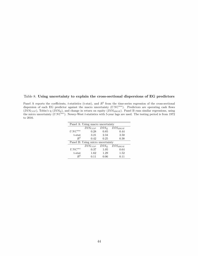
Table 8. Using uncertainty to explain the cross-sectional dispersions of EG predictors

Panel A reports the coefficients, t-statistics (t-stat), and R2 from the time-series regression of the cross-sectionaldispersion of each EG predictor against the macro uncertainty (UNCma). Predictors are operating cash flows(DISCOP ), Tobin’s q (DISQ), and change in return on equity (DISdROE). Panel B runs similar regressions, usingthe micro uncertainty (UNCmi). Newey-West t-statistics with 5-year lags are used. The testing period is from 1972to 2016.

Panel A: Using macro uncertainty

DISCOP DISQ DISdROE

UNCma 0.28 0.85 0.44t-stat 3.21 2.34 3.50R2 0.42 0.25 0.38

Panel B: Using micro uncertainty

DISCOP DISQ DISdROE

UNCmi 0.37 1.05 0.64t-stat 1.62 1.29 1.52R2 0.11 0.06 0.11

44

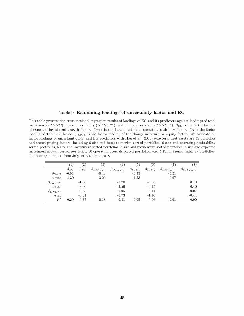
Table 9. Examining loadings of uncertainty factor and EG

This table presents the cross-sectional regression results of loadings of EG and its predictors against loadings of totaluncertainty (∆UNC), macro uncertainty (∆UNCma), and micro uncertainty (∆UNCmi). βEG is the factor loadingof expected investment growth factor. βCOP is the factor loading of operating cash flow factor. βQ is the factorloading of Tobin’s q factor. βdROE is the factor loading of the change in return on equity factor. We estimate allfactor loadings of uncertainty, EG, and EG predictors with Hou et al. (2015) q-factors. Test assets are 45 portfoliosand tested pricing factors, including 6 size and book-to-market sorted portfolios, 6 size and operating profitabilitysorted portfolios, 6 size and investment sorted portfolios, 6 size and momentum sorted portfolios, 6 size and expectedinvestment growth sorted portfolios, 10 operating accruals sorted portfolios, and 5 Fama-French industry portfolios.The testing period is from July 1973 to June 2018.

(1) (2) (3) (4) (5) (6) (7) (8)

βEG βEG βDISCOP βDISCOP βDISQ βDISQ βDISdROE βDISdROE

βUNC -0.91 -0.48 -0.33 -0.21t-stat -4.39 -3.20 -1.53 -0.67

βUNCma -1.08 -0.70 -0.05 0.19t-stat -3.60 -3.56 -0.15 0.40

βUNCmi -0.03 -0.05 -0.14 -0.07t-stat -0.31 -0.73 -1.16 -0.44R2 0.29 0.37 0.18 0.41 0.05 0.06 0.01 0.00

45

Table 10. Explaining the EG factor with uncertainty-augmented factor models

Panel A presents the abnormal returns and the factor loadings of EG factor from various macro uncertainty(∆UNCma)-augmented factor models, using the full sample. Panel B reports the abnormal returns and the fac-tor loadings of EG factor from various micro uncertainty (∆UNCmi)-augmented factor models. Factor modelsinclude the market model (CAPM), Fama and French (1993) three-factor model (FF3), Carhart (1997) four-factormodel (FF4), Fama and French (2015) five-factor model (FF5), Fama and French (2018) six-factor model (FF6),Stambaugh and Yuan (2017) model (SY), and Hou et al. (2015) q-factor model (HXZ). All returns are multipliedwith 100. Newey-West adjusted t-statistics (t-stat) with 6-month lags are provided. R2 denotes the explanatorypower of the corresponding factor model. The testing period is from July 1973 to June 2018.

Panel A: Factor models augmented by macro uncertainty

αRaw 0.81

t-stat 8.77α MKT ∆UNCma R2

CAPM 0.15 -0.06 -0.85 0.88t-stat 3.74 -6.31 -24.77

α MKT SMB HML ∆UNCma R2

FF3 0.01 -0.08 0.19 -0.06 -1.00 0.94t-stat 0.31 -10.83 20.27 -6.46 -51.24

α MKT SMB HML UMD ∆UNCma R2

FF4 0.01 -0.07 0.18 -0.05 0.03 -0.97 0.94t-stat 0.26 -11.24 18.94 -4.12 2.71 -47.55

α MKT SMB HML CMA RMW ∆UNCma R2

FF5 0.00 -0.09 0.22 0.01 -0.20 0.04 -1.04 0.96t-stat 0.05 -13.89 17.5 0.79 -7.69 1.86 -54.05

α MKT SMB HML CMA RMW UMD ∆UNCma R2

FF6 0.00 -0.09 0.21 0.03 -0.20 0.04 0.03 -1.01 0.96t-stat -0.04 -14.33 20.20 2.20 -9.26 2.26 4.47 -62.10

α MKT MISPME MGMT PERF ∆UNCma R2

HXZ -0.01 -0.09 0.22 -0.21 0.06 -1.05 0.98t-stat -0.52 -21.00 28.33 -15.85 5.77 -84.38

α MKT QME QIA QROE ∆UNCma R2

SY 0.00 -0.08 0.18 -0.06 0.05 -0.94 0.95t-stat -0.04 -8.93 16.16 -4.27 5.20 -54.10

46

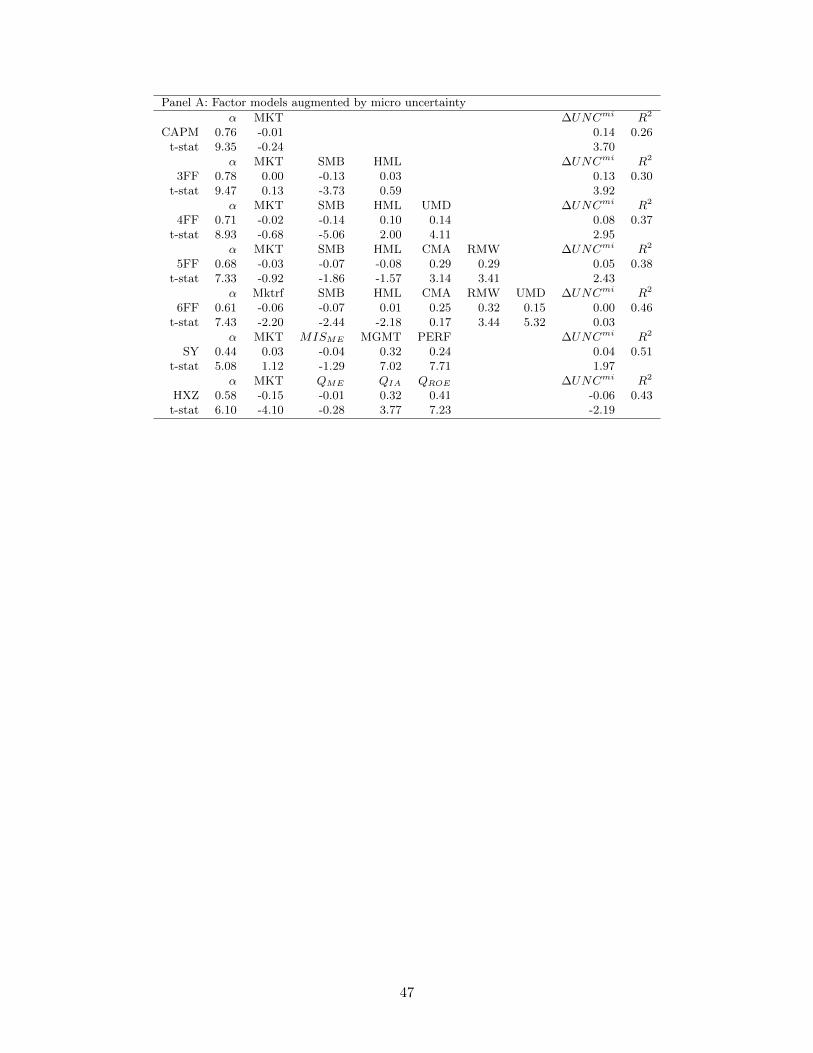
Panel A: Factor models augmented by micro uncertainty

α MKT ∆UNCmi R2

CAPM 0.76 -0.01 0.14 0.26t-stat 9.35 -0.24 3.70

α MKT SMB HML ∆UNCmi R2

3FF 0.78 0.00 -0.13 0.03 0.13 0.30t-stat 9.47 0.13 -3.73 0.59 3.92

α MKT SMB HML UMD ∆UNCmi R2

4FF 0.71 -0.02 -0.14 0.10 0.14 0.08 0.37t-stat 8.93 -0.68 -5.06 2.00 4.11 2.95

α MKT SMB HML CMA RMW ∆UNCmi R2

5FF 0.68 -0.03 -0.07 -0.08 0.29 0.29 0.05 0.38t-stat 7.33 -0.92 -1.86 -1.57 3.14 3.41 2.43

α Mktrf SMB HML CMA RMW UMD ∆UNCmi R2

6FF 0.61 -0.06 -0.07 0.01 0.25 0.32 0.15 0.00 0.46t-stat 7.43 -2.20 -2.44 -2.18 0.17 3.44 5.32 0.03

α MKT MISME MGMT PERF ∆UNCmi R2

SY 0.44 0.03 -0.04 0.32 0.24 0.04 0.51t-stat 5.08 1.12 -1.29 7.02 7.71 1.97

α MKT QME QIA QROE ∆UNCmi R2

HXZ 0.58 -0.15 -0.01 0.32 0.41 -0.06 0.43t-stat 6.10 -4.10 -0.28 3.77 7.23 -2.19

47

Tab

le11

.M

axim

um

square

dSharp

era

tio

Panel

Apre

sents

the

maxim

um

square

dSharp

era

tio

(Sh2(f

))of

the

tangen

tp

ort

folio

const

ruct

edby

pri

cing

fact

ors

from

pre

vailin

gfa

ctor

model

sand

macr

ounce

rtain

ty(∆UNC

ma)

augm

ente

dfa

ctor

model

s.P

anel

sB

and

Cre

port

sim

ilar

resu

lts,

usi

ng

mic

rounce

rtain

ty(∆UNC

mi),

or

tota

lunce

rtain

ty(∆UNC

)augm

ente

dfa

ctor

model

s,re

spec

tivel

y.F

act

or

model

sin

clude

Fam

aand

Fre

nch

(1993)

thre

e-fa

ctor

model

(FF

3),

Carh

art

(1997)

four-

fact

or

model

(FF

4),

Fam

aand

Fre

nch

(2015)

five-

fact

or

model

(FF

5),

Fam

aand

Fre

nch

(2018)

six-f

act

or

model

(FF

6),

Hou

etal.

(2015)q-

fact

or

model

(HX

Z),

and

Hou

etal.

(2021)q5

model

(HM

XZ

).T

he

5th

and

95th

per

centi

les

of

theSh2(f

)dis

trib

uti

on

from

ab

oots

trap

sim

ula

tion

of

10,0

00

tim

esare

rep

ort

edin

bra

cket

s.T

he

test

ing

per

iod

isfr

om

July

1973

toJune

2018.

Panel

A:

Pre

valing

fact

or

model

sand

∆UNC

ma

augm

ente

dfa

ctor

model

s

FF

3F

F3+

∆UNC

ma

FF

4F

F4+

∆UNC

ma

FF

5F

F5+

∆UNC

ma

Sh2(f

)0.0

40.2

00.0

80.2

30.1

10.2

4

(5th

,95th

)(0

.02,

0.0

9)

(0.1

4,

0.3

0)

(0.0

5,

0.1

5)

(0.1

6,

0.3

4)

(0.0

8,

0.1

8)

(0.1

8,

0.3

4)

FF

6F

F6+

∆UNC

ma

HX

ZH

XZ

+∆UNC

ma

HM

XZ

Sh2(f

)0.1

40.2

60.1

60.2

70.3

0

(5th

,95th

)(0

.10,

0.2

2)

(0.1

9,

0.3

8)

(0.1

1,

0.2

4)

(0.1

9,

0.3

8)

(0.2

3,

0.4

1)

Panel

B:

∆UNC

mi

augm

ente

dfa

ctor

model

s

FF

3+

∆UNC

mi

FF

4+

∆UNC

mi

FF

5+

∆UNC

mi

FF

6+

∆UNC

mi

HX

Z+

∆UNC

mi

Sh2(f

)0.0

50.0

90.1

10.2

60.2

7

(5th

,95th

)(0

.02,

0.0

9)

(0.0

5,

0.1

6)

(0.0

8,

0.1

8)

(0.1

9,

0.3

7)

(020,

0.3

8)

Panel

C:

∆UNC

augm

ente

dfa

ctor

model

sF

F3+

∆UNC

FF

4+

∆UNC

FF

5+

∆UNC

FF

6+

∆UNC

HX

Z+

∆UNC

Sh2(f

)0.1

80.0

90.1

20.1

50.1

9

(5th

,95th

)(0

.12,

0.2

6)

(0.0

6,

0.1

6)

(0.0

8,

0.1

9)

(0.1

0,

0.2

3)

(0.1

3,

0.2

7)

48

Online Appendices

A. A production economy with uncertainty shocks

Consider an all-equity representative firm, operating in discrete time with infinite horizon. The

firm generates output according to a constant returns to scale production function: Yt = XtKt.

Yt and Xt are the firm’s output and total factor productivity at time t, respectively. Kt is the

productive capital at the beginning of time t.

The logarithmic productivity, lnXt, follows an AR(1) process, with a time-varying volatility:

lnXt+1 = ρx lnXt + σtεx,t+1, (1)

σ2t+1 = (1− ρσ)σ2 + ρσσ

2t + υεσ,t+1, (2)

where 0 < ρx < 1 and 0 < ρσ < 1 are the coefficients, σ2 is the long-run average volatility, υ is a

constant, εx,t+1 and εσ,t+1 are the i.i.d. N(0, 1) exogenous shocks. Eq. (2) assumes a stochastic

volatility process (see, e.g., Fernandez-Villaverde and Guerron-Quintana (2020)), which describes

the macro uncertainty shocks. Similar to Bansal and Yaron (2004), for analytical tractability, we

assume an AR(1) process for the uncertainty.24

Productive capital evolves as Kt+1 = It + (1 − δ)Kt, with a quadratic capital adjustment cost

of a2

(ItKt

)2Kt, where It is investment at time t, δ is the depreciation rate, and a is a constant. The

dividend is given by Dt = Yt − It − a2

(ItKt

)2Kt.

To be simple, we assume a representative household with a power utility.25 The household

consumes the dividends to maximize her expected utility, as follows:

maxCt∞t=0

E∞∑t=0

βtC1−γt

1− γ(3)

Ct = Yt − It −a

2

(ItKt

)2

Kt, ∀t = 0, 1, 2... (4)

where γ is her relative risk aversion level and Ct is her consumption at time t.

24One unappealing feature of this assumption is the negative realizations of volatility. But, this assumption can beeasily relaxed, e.g., assuming the logarithmic volatility satisfies an AR(1) process in a numerical model.

25Using recursive preferences might make uncertainty shocks more important for asset prices.

49

The first-order condition gives

1 + aItKt

= Et

β

(Ct+1

Ct

)−γ [Xt+1 +

a

2

(It+1

Kt+1

)2

+ (1− δ)[1 + a

(It+1

Kt+1

)]]. (5)

The above equation says that the marginal costs of adding one additional unit of productive capital

equals its marginal benefits. This defines the marginal q at time t as follows:

qt ≡ 1 + aItKt. (6)

The real investment return, RIt+1, is:

RIt+1 =Xt+1 + a

2

(It+1

Kt+1

)2+ (1− δ)

[1 + a

(It+1

Kt+1

)]1 + a It

Kt

. (7)

Cochrane (1991) and Restoy and Rockinger (1994) show that stock returns equal real investment

returns when production is constant returns to scale. Therefore, Eq. (7) also computes stock

returns, Rt+1.

We can rewrite Eq. (5) as the basic asset pricing equation:

Et[Mt+1Rt+1] = 1, (8)

where the pricing kernel Mt+1 = β(Ct+1

Ct

)−γ.

To obtain the economic insights and for tractability, we consider a log-linearized version of the

economy. Let Vt denote logarithmic deviations of variable V from its steady state. Given the

three state variables (i.e., productivity Xt, productive capital Kt, and uncertainty σ2t ), the optimal

investment can be approximated as:

It = I0 + IxXt + IkKt + Iσσ2t , (9)

where I0, Ix, Ik, and Iσ are coefficients to be determined.

50

Log-linearizing Eq. (7) gives the expected return:

Et[Rt+1] = [h(Ik − 1)δ + h− 1]I0 + hIσ(1− ρσ)σ2

+

[h

aδρx + h (Ik − 1) δIx + hIxρx −

aδ

1 + aδIx

]Xt︸ ︷︷ ︸

prductivity shock

+

[h (Ik − 1) (1− δ + δIk)−

aδ

1 + aδ(Ik − 1)

]Kt︸ ︷︷ ︸

capital stock

+

[h (Ik − 1) δIσ + hIσρσ −

aδ

1 + aδIσ

]σ2t︸ ︷︷ ︸

uncertainty shock

, (10)

where h = aδ2−a

2δ2+(a−1)δ

. That is, uncertainty shocks affect stock returns.

Log-linearizing the resource constraint Eq. (4) gives

Ct =

[g −

(I

C+ gaδ2

)Ix

]Xt +

[g(

1 +a

2δ2)−(I

C+ gaδ2

)Ik

]Kt

−(I

C+ gaδ2

)Iσσ

2t +

(I

C+ gaδ2

)I0, (11)

where g = C+IC(1−a

2δ2)

. C and I are the steady state values, satisfying

I

C=

δ

1− a2δ

2 − δ. (12)

Therefore, g = 11−a

2δ2−δ > 0.

Log-linearizing the first-order condition Eq. (8) gives

− γ(EtCt+1 − Ct

)+ EtRt+1 +

1

2V art

[−γCt+1 + Rt+1

]= 0. (13)

This takes into account the impacts of uncertainty on quantities and asset prices (see, e.g., Malkho-

zov (2014) and Bianchi et al. (2018)).

Substituting Eq. (10) and (11) into (13) and matching the coefficients, we can solve for I0, Ix,

51

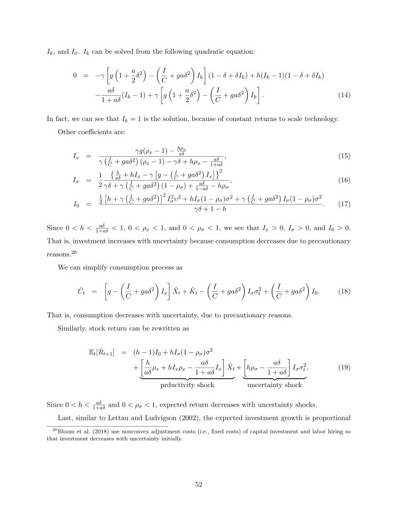
Ik, and Iσ. Ik can be solved from the following quadratic equation:

0 = −γ[g(

1 +a

2δ2)−(I

C+ gaδ2

)Ik

](1− δ + δIk) + h(Ik − 1)(1− δ + δIk)

− aδ

1 + aδ(Ik − 1) + γ

[g(

1 +a

2δ2)−(I

C+ gaδ2

)Ik

]. (14)

In fact, we can see that Ik = 1 is the solution, because of constant returns to scale technology.

Other coefficients are:

Ix =γg(ρx − 1)− hρx

aδ

γ(IC + gaδ2

)(ρx − 1)− γδ + hρx − aδ

1+aδ

, (15)

Iσ =1

2

haδ + hIx − γ

[g −

(IC + gaδ2

)Ix]2

γδ + γ(IC + gaδ2

)(1− ρσ) + aδ

1−aδ − hρσ, (16)

I0 =12

[h+ γ

(IC + gaδ2

)]2I2συ

2 + hIσ(1− ρσ)σ2 + γ(IC + gaδ2

)Iσ(1− ρσ)σ2

γδ + 1− h. (17)

Since 0 < h < aδ1+aδ < 1, 0 < ρx < 1, and 0 < ρσ < 1, we see that Ix > 0, Iσ > 0, and I0 > 0.

That is, investment increases with uncertainty because consumption decreases due to precautionary

reasons.26

We can simplify consumption process as

Ct =

[g −

(I

C+ gaδ2

)Ix

]Xt + Kt −

(I

C+ gaδ2

)Iσσ

2t +

(I

C+ gaδ2

)I0. (18)

That is, consumption decreases with uncertainty, due to precautionary reasons.

Similarly, stock return can be rewritten as

Et[Rt+1] = (h− 1)I0 + hIσ(1− ρσ)σ2

+

[h

aδρx + hIxρx −

aδ

1 + aδIx

]Xt︸ ︷︷ ︸

prductivity shock

+

[hρσ −

aδ

1 + aδ

]Iσσ

2t︸ ︷︷ ︸

uncertainty shock

, (19)

Since 0 < h < aδ1+aδ and 0 < ρσ < 1, expected return decreases with uncertainty shocks.

Last, similar to Lettau and Ludvigson (2002), the expected investment growth is proportional

26Bloom et al. (2018) use nonconvex adjustment costs (i.e., fixed costs) of capital investment and labor hiring sothat investment decreases with uncertainty initially.

52

to the expected growth rate of q, as follows

Et

[ˆIt+1

Kt+1− ItKt

]=

1 + aδ

aδEt [qt+1 − qt]

= Iσ(1− ρσ)σ2 + (ρx − 1) IxXt + (ρσ − 1) Iσσ2t . (20)

Since Iσ > 0 and 0 < ρσ < 1, the expected investment growth decreases with uncertainty shocks

(σ2t ). Taking Eq. (19) and (20) together, we see that the expected investment growth captures

uncertainty shocks and therefore it captures expected stock returns. That is, expected return

increases with expected investment growth.

B. TFP estimation

(1) Data

We use two main datasets to estimate the total factor productivity (TFP): Annual Compustat

and CRSP files, by matching Compustat and CRSP. The sample period is from 1966 to 2016.

Compustat items used include total assets (AT), net property, plant, and equipment (PPENT), sales

(SALE), operating income before depreciation (OIBDP), depreciation (DP), capital expenditure

(CAPX), inventory (INVT), sale of property, plant, and equipment (SPPE), depreciation, depletion

and amortization (DPACT), employees (EMP), and staff expense (XLR).

We apply several filters to select the sample firms. We include common stocks listed at

NYSE/Amex/Nasdaq. We exclude the financial firms and the utility firms (four-digit SIC be-

tween 6000 - 6999 or 4900 - 4999). Also, firms with sales or total assets less than $1 millions,

or with negative or missing book equity, employees, capital expenditure, and depreciation are ex-

cluded. Firms with negative value-added or material costs are excluded as well. Stock price of each

firm must be greater than $5 at the end of a year. The labor expense ratio, which we will describe

below, should be between 0 and 1. Following Chen and Chen (2012), we exclude firms with asset or

sales growth rate exceeding 100% to avoid potential business discontinuities that might be caused

by mergers and acquisitions. Finally, the sample firms should report their accounting information

more than 2 years to avoid the survivorship bias.

To calculate real values, we use GDP deflator (NIPA table 1.1.9 qtr line1) and price index for

nonresidential private fixed investment(NIPA table 5.3.4 qtr line2). We obtain employees’ earnings

data from Bureau of Labor Statistics (CES0500000030). This table reports weekly earnings for

each month. We use these to compute the annual earnings.

53

(2) Input variables

We calculate value-added, employment, physical capital, and investment to estimate TFP.

Value-added (Yit) is Salesit−MaterialsitGDP deflator . Material cost (Materialsit) is total expenses minus

labor expense. Total expense is sales (SALE) minus operating income before depreciation and

amortization (OIBDP). Labor expense is the staff expense (XLR). However, only a small number

of firms report the staff expense. We replace the missing observations with the interaction of

industry average labor expense ratio and total expense. To be specific, we calculate the labor

expense ratio, xlritsalesit−oibdpit , for each firm. Next, in each year we estimate the industry average of

the labor expense ratio at 4-digit SIC code level if there are at least 3 firms. Otherwise, we estimate

the industry average of the labor expense ratio at 3-digit SIC code level. In the same manner, we

estimate the industry average of labor expense ratio at 2-digit and 1-digit SIC code level. Then,

we back out the staff expense by multiplying the industry average labor expense ratio and total

expense. If the labor expense is still missing, we interpolate those missing observations with the

interaction of annual wage from the Bureau of Labor Statistics and the number of employees.

Capital stock (Kit) is net property, plant, and equipment divided by the capital price deflator.

We calculate the capital price deflator, following Imrohoroglu and Tuzel (2014). First, we compute

the age of capital in each year. Age of capital stock is dpactitdpit

. We further take a 3-year moving

average to smooth the capital age. Then, we match the current capital stock with the price index

for private fixed investment at current year minus capital age. Finally, we take one-year lag for the

capital stock to measure the available capital stock at the beginning of the period.

Investment (Iit) is capital expenditure (CAPX) minus sale of property, plant, and equipment

(SPPE) plus a change of inventory (INVT), INV Tit − INV Tit−1, deflated by current fixed invest-

ment price index. We replace missing observations of SPPE with 0.

Labor (Lit) is the number of employees.

(3) TFP estimation

We follow Olley and Pakes (1996) to estimate the total factor productivity (TFP). Olley and

Pakes (1996) provide a robust way to measure production function parameters, solving the simul-

taneity problem and selection bias. Olley and Pakes (1996) estimate the labor coefficient and the

capital coefficient separately to avoid the simultaneity problem. Also, they include the exit prob-

ability in TFP estimation process to avoid the selection bias. Imrohoroglu and Tuzel (2014) show

how to estimate Olley and Pakes (1996) TFP using annual Compustat and share their codes.27 We

27Available at http://www-bcf.usc.edu/ tuzel/TFPUpload/Programs/

54

follow Imrohoroglu and Tuzel (2014) with some modifications.

We start from the simple Cobb-Douglas production technology,

Yit = ZitLβLit K

βKit , (21)

where Yit, Zit, Lit, and Kit, are value-added, productivity, labor, and capital stock of a firm i at

time t. We scale the production function by its capital stock for several reasons. First, since TFP is

the residual term, it is often highly correlated with the firm size. Second, this avoids estimating the

capital coefficient directly. Third, there is an upward bias in labor coefficient without scaling. After

being scaled by the capital stock and transformed into logarithmic values, Eq.(21) is rewritten as

LogYitKit

= βLLogLitKit

+ (βK + βL − 1)LogKit + LogZit. (22)

We define Log YitKit, Log Lit

Kit, LogKit, and LogZit as ykit, lkit, kit, and zit. Also, denote βL and

(βK + βL − 1) as βl and βk. Rewrite Eq.(22) as

ykit = βllkit + βkkit + zit. (23)

Olley and Pakes (1996) assume a monotonic relationship between the investment and productiv-

ity (i.e., investment captures information of productivity). Hence, productivity is a function of

investment, i.e., zit = h(ikit). We assume that the function h(ikit) is 2nd-order polynomials of ikit.

Specifically, we estimate the following cross-sectional regression at the first stage:

yit = βllkit + βkkit + β0 + βikikit + βik2ik2it + year ∗ ηj + εit, (24)

where h(ikit) = β0 + βikikit + βik2ik2it. We include the interaction between year and industry (ηj)

fixed effect to capture the differences of industrial technologies over time. ηj is Fama-French 10

industry classification. From this stage, we estimate the labor coefficients, βl.

Second, the conditional expectation of y/ki,t+1 − βll/ki,t+1 − year ∗ ηj on information at t and

survival of the firm is

Et(yki,t+1 − βllki,t+1 − year ∗ ηj) = βkki,t+1 + Et(zi,t+1|zi,t, survival)

= βkki,t+1 + g(zit, Psurvival,t),(25)

55

where Psurvival,t is the probability of a firm survival from t to t+1. The probability is estimated

with the Probit regression of a survival indicator variable on the 2nd polynomials in investment

rate, i/k. zit is β0 + βikikit + βik2ik2it. The function g is the polynomials of the survival probability

(Psurvival,t) and lagged TFP (zit). At this step, we estimate the coefficient of capital, βk, which

gives βK .

From the second stage, total factor productivity (TFP) can be computed as follows:

TFPit = exp(ykit − βllki,t − (βK + βl − 1)kit − year ∗ ηj). (26)

After transforming the exponential values, we estimate TFP growth, TFPit−TFPit−1

TFPt−1. We use a

5-year rolling window to estimate TFP. TFP estimates are available from 1972 to 2016.

C. Cross-sectional regressions of factor models augmented with uncertainty factors

In this section, we consider three variations of uncertainty augmented factor models. That is,

prevailing factor models augmented by the total uncertainty factor, macro and micro uncertainty

factors, and the aggregate uncertainty factor.

C.1. Cross-sectional regressions of factor models augmented with total uncertainty factor

Since ∆UNCma tracks ∆UNC, we can replace ∆UNCma with ∆UNC and run the Fama-

MacBeth regressions. Panel A of Table C1 reports the results with the full-sample estimation,

which are qualitatively similar to those reported in Table 5. γ0 from the augmented FF6 and

SY models are insignificant. Also, γUNC are significantly negative across all models and their

magnitudes are close to the average factor return. To avoid the look-ahead bias, we report Fama-

MacBeth regressions using the extending-window estimation in Panel B of Table C1. The testing

period is from July 1997 to June 2018. We find similar results in the extending-window cases. First,

γUNC is significantly negative across all augmented factor models. Second, the intercepts become

smaller or insignificant after we add ∆UNC to the prevailing factor models.

C.2. Cross-sectional regressions of factor models augmented with macro and micro uncertainty

factor

For another robustness check, we extend the prevailing factor models by adding both ∆UNCma

and ∆UNCmi, and report results in Table C2. We see that across the augmented factor models,

56

only γUNCma are significantly negative while γUNCmi are insignificant. The augmented FF3, FF4,

FF5, FF6, HXZ, and SY models have insignificant pricing errors in the full-sample estimation

reported in Panel A. Panel B shows the extending-window estimation results, which are similar to

those in Panel A.

C.3. Cross-sectional regressions of factor models augmented with aggregate uncertainty factors

Table C3 reports Fama-MacBeth regressions of various factor models augmented with the

mimicking aggregate uncertainty portfolio (UNCagg), using full sample. Aggregate uncertainty

(UNCagg) is the conditional standard deviation of a GARCH (1,1) on aggregate TFP. Table C3

shows that the mimicking aggregate uncertainty portfolio is negatively priced, but the augmented

models have significant intercepts. Overall, we see that the macro uncertainty factor (UNCma)

performs better than the mimicking aggregate uncertainty factor (UNCagg).

Table C4 reports Fama-MacBeth regressions of various factor models augmented with the mim-

icking VIX portfolio (∆V IX), using full sample. Again, we see that the mimicking VIX portfolio is

negatively priced. The augmented FF6 model has an insignificant intercept but other augmented

models have significant pricing errors. Overall, we see that the macro uncertainty factor (UNCma)

performs better than the mimicking VIX factor.

D. Explaining the expected investment growth factor with total uncertainty-augmented fac-

tor models

To avoid the look-ahead bias, we use the extending-window to decompose EG into predicted

and residual components. Starting from 1985, we regress the firm-level EG against the macro

uncertainty to compute these two components over time. We sort all stocks into decile portfolios

based on either their predicted EG or residual EG. Portfolio 10 (1) has the highest (lowest) predicted

or residual EG. We compute the value-weighted portfolio returns and the alphas from various asset

pricing models. Panel A of Table D1 shows that portfolio returns increase with predicted EG.

The long-short portfolio has a significantly positive alpha from all benchmark models. But Panel

B of Table D1 shows that the residual EG doesn’t provide additional information. For example,

the long-short portfolio has much smaller alphas than those reported in Panel A and its alpha

is insignificant from SY model. Overall, we see that the pricing of EG is driven by the macro

uncertainty risk.

57

E. Explaining the cross-sectional dispersions of EG predictors with total uncertainty

Table E1 presents the univariate regression of the cross-sectional dispersion of each EG predictor

against the total uncertainty (UNC). EG predictors are operating cash flows (COP), Tobin’s q

(Q), and change in return on equity (dROE). We see that UNC explains most of the cross-sectional

dispersions of EG predictors.

F. Explaining the pricing powers of three EG predictors

Table F1 compares the pricing powers of three EG predictors. We augment Hou et al. (2015)

q-factor model with each predictor of EG and run Fama-MacBeth regressions. We see that oper-

ating cash flows (COP ) and dROE are significantly positive, but Tobin’s q is insignificant. Also,

HXZ+COP has the highest R2. This is consistent with Hou et al. (2021) that future investment

growth is predicted mainly by COP .

G. Explaining the expected investment growth factor with total uncertainty-augmented fac-

tor models

Table G1 reports the regression coefficients of using ∆UNC to explain the EG factor. The full-

sample estimation results in Panel A show that ∆UNC captures the EG factor in augmented SY

model, with insignificant intercepts of 0.02% (t-statistic=0.32). ∆UNC are significantly negative

in all models.

To avoid the look-ahead bias, we presents similar regression results, using the extending-window

estimation, in Panel B. The results are similar to those reported in Panel A.

H. Comparing the q5 model with total uncertainty-augmented q-model

For the robustness check, we compare Hou et al. (2021) q5 model (HMXZ) with ∆UNC-

augmented HXZ model (HXZ+∆UNC) in Table H1. The results are similar to those using

∆UNCma in Table 5. Overall, the EG factor and ∆UNC have similar contribution in explaining

the test portfolios in the cross section.

58

References

Bansal, R., Yaron, A., 2004. Risks for the long run: A potential resolution of asset pricing puzzles.

Journal of Finance 59, 1481–1509.

Bianchi, F., Kung, H., Tirskikh, M., 2018. The origins and effects of macroeconomic uncertainty,

NBER Working Paper No. 25386.

Bloom, N., Floetotto, M., Jaimovich, N., Saporta-Eksten, I., Terry, S. J., 2018. Really uncertain

business cycles. Econometrica 86, 1031–1065.

Carhart, M. M., 1997. On persistence in mutual fund performance. Journal of Finance 52, 57–82.

Chen, H., Chen, S., 2012. Investment-cash flow sensitivity cannot be a good measure of financial

constraints: Evidence from the time series. Journal of Financial Economics 103, 393–410.

Cochrane, J. H., 1991. Production-based asset pricing and the link between stock returns and

economic fluctuation. Journal of Finance 46, 209–237.

Fama, E. F., French, K. R., 1993. Common risk factors in the returns on stocks and bonds. Journal

of Financial Economics 33, 3–56.

Fama, E. F., French, K. R., 2015. A five-factor asset pricing model. Journal of Financial Economics

116, 1–22.

Fama, E. F., French, K. R., 2018. Choosing factors. Journal of Financial Economics 128, 234–252.

Fernandez-Villaverde, J., Guerron-Quintana, P. A., 2020. Uncertainty shocks and business cycle

research, NBER Working Paper No. 26768.

Hou, K., Mo, H., Xue, C., Zhang, L., 2021. An augmented q-factor model with expected growth.

Review of Finance 25, 1–41.

Hou, K., Xue, C., Zhang, L., 2015. Digesting anomalies: An investment approach. Review of

Financial Studies 28, 650–705.

Imrohoroglu, A., Tuzel, Selale., 2014. Firm-level productivity, risk, and return. Management Science

60, 1861–2109.

Jagannathan, R., Wang, Z., 1996. The conditional CAPM and the cross-section of expected returns.

Journal of Finance 51, 3–53.

Lettau, M., Ludvigson, S., 2002. Time-varying risk premia and the cost of capital: An alternative

implication of the Q theory of investment. Journal of Monetary Economics 49, 31–66.

Malkhozov, A., 2014. Asset prices in affine real business cycle models. Journal of Economic Dy-

namics and Control 45, 180–193.

59

Olley, G. S., Pakes, A., 1996. The dynamics of productivity in the telecommunications equipment

industry. Econometrica 64, 1263–1297.

Restoy, F., Rockinger, G. M., 1994. On stock market returns and returns on investment. Journal

of Finance 49, 543–556.

Shanken, J., 1992. On the estimation of beta-pricing models. Review of Financial Studies 5, 1–55.

Stambaugh, R. F., Yuan, Y., 2017. Mispricing factors. Review of Financial Studies 30, 1270–1315.

60

Tab

leC

1.Cro

ss-sectionalre

gre

ssionsoffacto

rmodels

augmented

with

tota

luncertainty

facto

r

Panel

Are

port

sth

eco

effici

ents

(Coeff

)andt-

stati

stic

s(t

-sta

t)fr

om

Fam

a-M

acB

eth

regre

ssio

ns

of

vari

ous

fact

or

model

sand

fact

or

model

saugm

ente

dw

ith

tota

lunce

rtain

ty(∆UNC

),usi

ng

the

full-s

am

ple

esti

mati

on.

Tes

tass

ets

are

45

port

folios

and

the

test

edpri

cing

fact

ors

,in

cludin

g6

size

and

book-t

o-m

ark

etso

rted

port

folios,

6si

zeand

op

erati

ng

pro

fita

bilit

yso

rted

port

folios,

6si

zeand

inves

tmen

tso

rted

port

folios,

6si

zeand

mom

entu

mso

rted

port

folios,

6si

zeand

exp

ecte

din

ves

tmen

tgro

wth

sort

edp

ort

folios,

10

op

erati

ng

acc

rual

sort

edp

ort

folios,

and

5F

am

a-F

rench

indust

ryp

ort

folios.

Tes

ted

fact

or

model

sare

Fam

aand

Fre

nch

(1993)

thre

e-fa

ctor

model

(FF

3),

Carh

art

(1997)

four-

fact

or

model

(FF

4),

Fam

aand

Fre

nch

(2015)

five-

fact

or

model

(FF

5),

Fam

aand

Fre

nch

(2018)

six-f

act

or

model

(FF

6),

Hou

etal.

(2015)q-

fact

or

model

(HM

Z),

and

Sta

mbaugh

and

Yuan

(2017)

model

(SY

).P

anel

Bsh

ows

sim

ilar

resu

lts

inth

eex

tendin

g-w

indow

.A

llco

effici

ents

are

mult

iplied

by

100.

Thet-

stati

stic

sare

adju

sted

for

erro

rs-i

n-v

ari

able

s,fo

llow

ing

Shanken

(1992).

The

adju

sted

R2

follow

sJagannath

an

and

Wang

(1996).

The

5th

and

95th

per

centi

les

of

the

adju

sted

R2

dis

trib

uti

on

from

ab

oots

trap

sim

ula

tion

of

10,0

00

tim

esare

rep

ort

edin

bra

cket

s.T

he

test

ing

per

iod

for

Panel

Ais

from

July

1973

toJune

2018.

The

test

ing

per

iod

for

Panel

Bis

from

July

1997

toJune

2018.

Panel

A:

Full-s

am

ple

esti

mati

on

FF

3F

F3+

∆UNC

FF

4F

F4+

∆UNC

FF

5F

F5+

∆UNC

FF

6F

F6+

∆UNC

Coeff

t-st

at

Coeff

t-st

at

Coeff

t-st

at

Coeff

t-st

at

Coeff

t-st

at

Coeff

t-st

at

Coeff

t-st

at

Coeff

t-st

at

γ0

0.3

36.3

30.1

83.3

70.0

83.6

10.0

62.3

60.0

93.5

50.0

62.1

00.0

62.8

00.0

31.3

5γM

KT

0.2

91.4

60.4

12.0

50.5

62.8

70.5

52.8

00.5

02.5

50.5

22.6

20.5

62.8

60.5

72.8

9γSM

B0.1

91.4

70.2

41.8

00.2

31.7

40.2

51.9

00.2

72.1

00.2

82.1

20.2

72.0

90.2

82.1

2γH

ML

0.2

11.5

70.2

51.8

10.3

62.6

70.3

32.4

20.1

30.9

50.2

01.4

90.2

51.8

80.2

92.2

3γCM

A0.3

94.0

90.3

73.1

20.3

03.2

90.3

03.2

8γRM

W0.2

01.8

40.3

02.8

10.1

81.7

00.2

82.6

6γUM

D0.6

23.2

90.5

73.0

30.6

03.1

90.5

83.0

8γUN

C-1

.02

-8.6

2-0

.87

-8.3

0-0

.91

-8.3

9-0

.85

-8.0

4R

20.1

90.8

20.5

10.8

80.5

10.8

60.6

40.9

1

(5th

,95th

)(0

.02,

0.5

0)

(0.6

4,

0.8

8)

(0.3

3,

0.7

0)

(0.7

6,

0.9

1)

(0.2

9,

0.7

2)

(0.7

2,

0.9

1)

(0.4

6,

0.8

0)

(0.8

2,

0.9

3)

Panel

A(C

onti

nued

)

HX

ZH

XZ

+∆UNC

HM

XZ

SY

SY

+∆UNC

Coeff

t-st

at

Coeff

t-st

at

Coeff

t-st

at

Coeff

t-st

at

Coeff

t-st

at

γ0

0.1

12.8

10.0

71.9

20.0

72.1

00.0

81.6

00.0

51.0

4γM

KT

0.5

02.5

00.5

22.6

10.5

42.7

20.5

12.4

80.5

22.5

4γQ

ME

0.3

52.5

50.3

52.5

20.3

62.6

2γQ

IA

0.2

92.7

10.3

53.2

70.3

12.9

3γQ

RO

E0.4

53.3

20.3

92.8

20.3

32.4

0γEG

0.7

97.7

0γM

ISM

E0.4

03.0

60.4

63.5

3γM

GM

T0.5

33.5

70.5

23.4

7γPERF

0.5

52.9

30.6

03.1

8γUN

C-0

.86

-7.8

5-0

.84

-7.6

1R

20.5

10.9

10.8

20.7

00.9

1

(5th

,95th

)(0

.30,

0.7

1)

(0.8

0,

0.9

2)

(0.6

6,

0.8

7)

(0.5

1,

0.8

2)

(0.8

1,

0.9

2)

61

Pan

elB

:E

xte

nd

ing-

win

dow

esti

mat

ion

FF

3F

F3+

∆UNC

FF

4F

F4+

∆UNC

FF

5F

F5+

∆UNC

FF

6F

F6+

∆UNC

Coeff

t-st

atC

oeff

t-st

atC

oeff

t-st

atC

oeff

t-st

atC

oeff

t-st

atC

oeff

t-st

at

Coeff

t-st

at

Coeff

t-st

at

γ0

0.22

2.89

0.01

0.21

0.09

2.38

0.06

1.61

0.12

2.93

0.05

1.1

50.0

92.8

90.0

72.0

4γMKT

0.40

1.34

0.60

1.97

0.55

1.95

0.53

1.80

0.47

1.69

0.55

1.9

10.5

11.8

20.5

21.8

4γSMB

0.20

0.98

0.27

1.28

0.22

1.04

0.28

1.30

0.27

1.30

0.28

1.3

50.2

61.2

90.2

81.3

5γHML

0.14

0.61

0.22

0.90

0.23

0.99

0.17

0.74

0.03

0.15

0.16

0.7

20.0

80.3

70.1

30.6

0γCMA

0.22

1.23

0.15

0.8

50.1

81.1

10.1

60.9

2γRMW

0.13

0.59

0.19

0.8

80.1

60.7

60.2

00.9

1γUMD

0.42

1.21

0.35

0.96

0.3

91.1

30.3

50.9

7γUNC

-0.6

5-3

.04

-0.7

7-3

.82

-0.6

1-3

.17

-0.7

0-4

.25

R2

0.31

0.83

0.45

0.85

0.52

0.83

0.5

70.8

5(5th

,95th

)(0

.01,

0.61

)(0

.73,

0.92

)(0

.30,

0.76

)(0

.75,

0.93

)(0

.26,

0.78

)(0

.75,

0.93)

(0.4

3,

0.8

4)

(0.7

8,

0.9

4)

Pan

elB

(Con

tinu

ed)

HX

ZH

XZ

+∆UNC

HM

XZ

SY

SY

+∆UNC

Coeff

t-st

atC

oeff

t-st

atC

oeff

t-st

atC

oeff

t-st

atC

oeff

t-st

atγ

00.

121.

730.

050.

870.

060.

960.

131.

360.

121.

68γMKT

0.48

1.74

0.56

1.97

0.55

1.92

0.43

1.44

0.44

1.49

γQ

ME

0.30

1.45

0.33

1.54

0.32

1.46

γQ

IA

0.16

0.84

0.2

1.03

0.19

1.01

γQ

ROE

0.19

0.72

0.14

0.57

0.14

0.53

γEG

0.61

3.32

γMISM

E0.

371.

710.

391.

80γMGMT

0.44

1.77

0.40

1.49

γPERF

0.58

1.49

0.51

1.31

γUNC

-0.6

4-3

.58

-0.6

6-3

.95

R2

0.44

0.83

0.74

0.61

0.80

(5th

,95th

)(0

.25,

0.77

)(0

.72,

0.92

)(0

.60,

0.88

)(0

.45,

0.85

)(0

.73,

0.92

)

62

Tab

leC

2.Cro

ss-sectionalre

gre

ssionsofmacro

-and

micro

-uncertainty

augmented

facto

rmodels

Panel

Are

port

sF

am

a-M

acB

eth

regre

ssio

ns

of

vari

ous

fact

or

model

saugm

ente

dw

ith

both

macr

oand

mic

rounce

rtain

tyfa

ctors

,usi

ng

the

full-s

am

ple

esti

mati

on.

Panel

Bsh

ows

sim

ilar

resu

lts,

usi

ng

the

exte

ndin

g-w

indow

esti

mati

on.

Tes

tass

ets

are

45

port

folios

and

the

test

edpri

cing

fact

ors

,in

cludin

g6

size

and

book-t

o-

mark

etso

rted

port

folios,

6si

zeand

op

erati

ng

pro

fita

bilit

yso

rted

port

folios,

6si

zeand

inves

tmen

tso

rted

port

folios,

6si

zeand

mom

entu

mso

rted

port

folios,

6si

zeand

exp

ecte

din

ves

tmen

tgro

wth

sort

edp

ort

folios,

10

op

erati

ng

acc

rual

sort

edp

ort

folios,

and

5F

am

a-F

rench

indust

ryp

ort

folios.

Tes

ted

fact

or

model

sare

Fam

aand

Fre

nch

(1993)

thre

e-fa

ctor

model

(FF

3),

Carh

art

(1997)

four-

fact

or

model

(FF

4),

Fam

aand

Fre

nch

(2015)

five-

fact

or

model

(FF

5),

Fam

aand

Fre

nch

(2018)

six-f

act

or

model

(FF

6),

Hou

etal.

(2015)q-

fact

or

model

(HM

Z),

and

Sta

mbaugh

and

Yuan

(2017)

model

(SY

).A

llco

effici

ents

are

mult

iplied

by

100.

The

t-st

ati

stic

sare

adju

sted

for

erro

rs-i

n-v

ari

able

s,fo

llow

ing

Shanken

(1992).

The

adju

sted

R2

follow

sJagannath

an

and

Wang

(1996).

The

5th

and

95th

per

centi

les

of

the

adju

sted

R2

dis

trib

uti

on

from

ab

oots

trap

sim

ula

tion

of

10,0

00

tim

esare

rep

ort

edin

bra

cket

s.T

he

test

ing

per

iod

for

Panel

Ais

from

July

1973

toJune

2018.

The

test

ing

per

iod

for

Panel

Bis

from

July

1997

toJune

2018.

Panel

A:

Fact

or

model

saugm

ente

dw

ith

macr

o-

and

mic

ro-

unce

rtain

ty,

usi

ng

the

full-s

am

ple

esti

mati

on

FF

3+

∆UNC

ma,m

iF

F4+

∆UNC

ma,m

iF

F5+

∆UNC

ma,m

iF

F6+

∆UNC

ma,m

iH

XZ

+∆UNC

ma,m

iSY

+∆UNC

ma,m

i

Coeff

t-st

at

Coeff

t-st

at

Coeff

t-st

at

Coeff

t-st

at

Coeff

t-st

at

Coeff

t-st

at

γ0

0.0

20.6

20.0

20.9

40.0

31.2

40.0

31.4

60.0

51.6

30.0

71.5

8γM

KT

0.5

82.9

10.5

72.9

30.5

72.8

90.5

72.9

00.5

52.8

00.5

12.4

8γSM

B0.2

82.1

80.2

82.1

80.2

82.1

70.2

82.1

7γH

ML

0.2

92.0

90.2

92.1

40.3

02.2

30.3

02.2

7γCM

A0.2

82.9

70.2

82.9

8γRM

W0.2

42.2

30.2

42.2

3γUM

D0.5

73.0

40.5

73.0

2γQ

ME

0.3

72.6

7γQ

IA

0.3

53.3

8γQ

RO

E0.3

62.6

5γM

ISPM

E0.4

73.6

6γM

GM

T0.4

53.0

7γPERF

0.5

42.8

7γUN

Cm

a-0

.82

-7.2

3-0

.81

-7.9

7-0

.83

-7.7

0-0

.82

-8.5

8-0

.81

-7.9

1-0

.81

-8.2

0γUN

Cm

i-0

.22

-0.9

2-0

.23

-0.9

5-0

.23

-0.9

5-0

.23

-0.9

7-0

.25

-1.0

5-0

.26

-1.0

5R

20.9

20.9

20.9

20.9

20.9

10.9

1

(5th

,95th

)(0

.81,

0.9

3)

(0.8

2,

0.9

4)

(0.8

2,

0.9

4)

(0.8

4,

0.9

5)

(0.8

0,

0.9

3)

(0.8

1,

0.9

4)

63

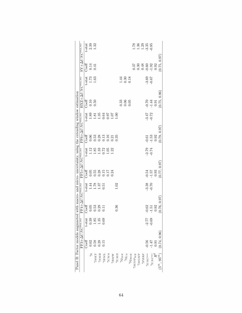
Panel

B:

Fact

or

model

saugm

net

edw

ith

macr

o-

and

mic

ro-

unce

rtain

ty,

usi

ng

the

exte

ndin

gw

indow

esti

mati

on

FF

3+

∆UNC

ma,m

iF

F4+

∆UNC

ma,m

iF

F5+

∆UNC

ma,m

iF

F6+

∆UNC

ma,m

iH

XZ

+∆UNC

ma,m

iSY

+∆UNC

ma,m

i

Coeff

t-st

at

Coeff

t-st

at

Coeff

t-st

at

Coeff

t-st

at

Coeff

t-st

at

Coeff

t-st

at

γ0

0.0

20.3

90.0

51.4

40.0

51.1

20.0

61.8

90.1

01.7

30.1

42.3

9γM

KT

0.5

81.8

50.5

31.7

80.5

51.8

50.5

31.8

10.5

01.6

30.4

11.3

2γSM

B0.2

81.3

50.2

91.3

70.2

81.3

30.2

81.3

5γH

ML

0.1

50.6

90.1

10.5

10.1

50.7

20.1

30.6

4γCM

A0.1

71.0

50.1

60.9

7γRM

W0.2

41.2

20.2

11.0

7γUM

D0.3

61.0

20.3

51.0

0γQ

ME

0.3

31.4

4γQ

IA

0.0

60.3

0γQ

RO

E0.0

50.1

8γM

ISPM

E0.3

71.7

8γM

GM

T0.3

01.3

6γPERF

0.4

81.2

9γUN

Cm

a-0

.56

-2.7

7-0

.62

-3.3

8-0

.54

-2.7

9-0

.61

-3.4

7-0

.70

-3.6

9-0

.60

-3.3

5γUN

Cm

i-1

.47

-0.6

9-1

.51

-0.7

0-1

.57

-0.7

4-1

.53

-0.7

2-1

.44

-0.6

7-1

.92

-0.9

5R

20.9

10.9

20.9

30.9

20.9

10.9

2

(5th

,95th

)(0

.74,

0.9

6)

(0.7

6,

0.9

7)

(0.7

7,

0.9

7)

(0.7

9,

0.9

7)

(0.7

5,

0.9

6)

(0.7

5,

0.9

7)

64

Tab

leC

3.Cro

ss-sectionalre

gre

ssionsofaggre

gate

uncertainty

-augmented

facto

rmodels

This

table

rep

ort

sF

am

a-M

acB

eth

regre

ssio

ns

of

vari

ous

fact

or

model

saugm

ente

dw

ith

the

mim

ickin

gaggre

gate

unce

rtain

typ

ort

folio

(∆UNC

agg),

usi

ng

full

sam

ple

.T

est

ass

ets

are

45

port

folios

and

the

test

edpri

cing

fact

ors

,in

cludin

g6

size

and

book-t

o-m

ark

etso

rted

port

folios,

6si

zeand

op

erati

ng

pro

fita

bilit

yso

rted

port

folios,

6si

zeand

inves

tmen

tso

rted

port

folios,

6si

zeand

mom

entu

mso

rted

port

folios,

6si

zeand

exp

ecte

din

ves

tmen

tgro

wth

sort

edp

ort

folios,

10

op

erati

ng

acc

rual

sort

edp

ort

folios,

and

5F

am

a-F

rench

indust

ryp

ort

folios.

Tes

ted

fact

or

model

sare

Fam

aand

Fre

nch

(1993)

thre

e-fa

ctor

model

(FF

3),

Carh

art

(1997)

four-

fact

or

model

(FF

4),

Fam

aand

Fre

nch

(2015)

five-

fact

or

model

(FF

5),

Fam

aand

Fre

nch

(2018)

six-f

act

or

model

(FF

6),

Hou

etal.

(2015)q-

fact

or

model

(HM

Z),

and

Sta

mbaugh

and

Yuan

(2017)

model

(SY

).A

llco

effici

ents

are

mult

iplied

by

100.

The

t-st

ati

stic

sare

adju

sted

for

erro

rs-i

n-v

ari

able

s,fo

llow

ing

Shanken

(1992).

The

adju

sted

R2

follow

sJagannath

an

and

Wang

(1996).

The

5th

and

95th

per

centi

les

of

the

adju

sted

R2

dis

trib

uti

on

from

ab

oots

trap

sim

ula

tion

of

10,0

00

tim

esare

rep

ort

edin

bra

cket

s.T

he

test

ing

per

iod

isfr

om

July

1973

toJune

2018.

FF

3+

∆UNC

agg

FF

4+

∆UNC

agg

FF

5+

∆UNC

agg

FF

6+

∆UNC

agg

HX

Z+

∆UNC

agg

SY

+∆UNC

agg

Coeff

t-st

at

Coeff

t-st

at

Coeff

t-st

at

Coeff

t-st

at

Coeff

t-st

at

Coeff

t-st

at

γ0

0.2

34.4

40.1

13.3

40.1

24.1

60.0

93.6

70.1

43.4

60.0

71.7

3γM

KT

0.3

51.7

10.4

92.4

90.4

52.3

00.5

12.5

80.4

52.2

40.4

92.4

2γSM

B0.2

82.1

30.2

92.1

90.2

92.2

40.2

92.2

3γH

ML

0.2

31.6

90.3

22.3

60.2

01.4

70.3

12.3

8γCM

A0.3

53.5

90.2

62.7

9γRM

W0.2

01.8

90.1

91.7

4γUM

D0.5

52.9

00.5

62.9

6γQ

ME

0.3

92.8

2γQ

IA

0.3

33.0

7γQ

RO

E0.3

12.2

3γM

ISM

E0.4

93.8

0γM

GM

T0.5

33.6

6γPERF

0.5

63.0

0γUN

Cagg

-1.0

5-7

.94

-0.9

3-7

.36

-0.9

3-7

.79

-0.9

0-7

.61

-0.8

8-7

.24

-0.7

9-6

.28

R2

0.7

70.8

60.7

80.8

60.8

10.8

7

(5th

,95th

)(0

.56,

0.8

5)

(0.7

4,

0.9

0)

(0.6

0,

0.8

7)

(0.7

5,

0.9

1)

(0.6

5,

0.8

8)

(0.7

4,

0.9

1)

65

Tab

leC

4.Cro

ss-sectionalre

gre

ssionsofth

emim

ickinguncertainty

augmented

models:UsingVIX

index

This

table

rep

ort

sF

am

a-M

acB

eth

regre

ssio

ns

of

vari

ous

fact

or

model

sand

those

augm

ente

dw

ith

the

mim

ickin

gunce

rtain

tyfa

ctor

usi

ng

VIX

index

(∆VIX

),usi

ng

the

full-s

am

ple

esti

mati

on.

Tes

tass

ets

are

45

port

folios

and

the

test

edpri

cing

fact

ors

,in

cludin

g6

size

and

book-t

o-m

ark

etso

rted

port

folios,

6si

zeand

op

erati

ng

pro

fita

bilit

yso

rted

port

folios,

6si

zeand

inves

tmen

tso

rted

port

folios,

6si

zeand

mom

entu

mso

rted

port

folios,

6si

zeand

exp

ecte

din

ves

tmen

tgro

wth

sort

edp

ort

folios,

10

op

erati

ng

acc

rual

sort

edp

ort

folios,

and

5F

am

a-F

rench

indust

ryp

ort

folios.

Tes

ted

fact

or

model

sare

Fam

aand

Fre

nch

(1993)

thre

e-fa

ctor

model

(FF

3),

Carh

art

(1997)

four-

fact

or

model

(FF

4),

Fam

aand

Fre

nch

(2015)

five-

fact

or

model

(FF

5),

Fam

aand

Fre

nch

(2018)

six-f

act

or

model

(FF

6),

Hou

etal.

(2015)q-

fact

or

model

(HM

Z),

Hou

etal.

(2021),

and

Sta

mbaugh

and

Yuan

(2017)

model

(SY

).A

llco

effici

ents

are

mult

iplied

by

100.

Thet-

stati

stic

sare

adju

sted

for

erro

rs-i

n-v

ari

able

s,fo

llow

ing

Shanken

(1992).

The

adju

sted

R2

follow

sJagannath

an

and

Wang

(1996).

The

5th

and

95th

per

centi

les

of

the

adju

sted

R2

dis

trib

uti

on

from

ab

oots

trap

sim

ula

tion

of

10,0

00

tim

esare

rep

ort

edin

bra

cket

s.T

he

test

ing

per

iod

isJuly

1988

toJune

2018.

FF

3F

F3+

∆VIX

FF

4F

F4+

∆VIX

FF

5F

F5+

∆VIX

FF

6F

F6+

∆VIX

Coeff

t-st

at

Coeff

t-st

at

Coeff

t-st

at

Coeff

t-st

at

Coeff

t-st

at

Coeff

t-st

at

Coeff

t-st

at

Coeff

t-st

at

γ0

0.4

45.3

20.4

35.7

60.1

33.7

90.1

74.6

70.0

82.7

70.0

92.6

70.0

41.6

30.0

62.0

9γM

KT

0.2

61.1

10.2

51.0

60.6

02.7

00.5

32.4

00.5

82.5

90.5

62.5

00.6

52.9

50.6

22.7

9γSM

B0.0

60.3

60.0

60.3

50.0

90.5

50.0

80.5

20.1

50.9

50.1

40.8

90.1

50.9

60.1

40.8

7γH

ML

0.0

80.4

70.1

20.6

90.2

41.4

50.2

51.5

0-0

.04

-0.2

6-0

.02

-0.1

00.0

80.4

70.1

10.6

9γCM

A0.2

82.2

90.3

12.5

40.2

11.7

70.2

31.9

1γRM

W0.2

92.0

70.3

42.3

90.2

81.9

60.3

12.2

1γUM

D0.5

62.3

00.5

32.1

60.5

72.3

30.5

62.2

5γVIX

-1.1

3-7

.38

-1.0

3-6

.86

-0.9

0-5

.86

-0.9

3-6

.15

R2

0.0

30.5

80.3

80.8

10.5

20.8

00.6

60.9

1

(5th

,95th

)(-

0.0

3,

0.4

7)

(0.3

3,

0.7

8)

(0.2

4,

0.6

7)

(0.6

3,

0.8

8)

(0.3

0,

0.7

6)

(0.6

0,

0.9

0)

(0.4

9,

0.8

3)

(0.7

9,

0.9

4)

HX

ZH

XZ

+∆VIX

HM

XZ

SY

SY

+∆VIX

Coeff

t-st

at

Coeff

t-st

at

Coeff

t-st

at

Coeff

t-st

at

Coeff

t-st

at

γ0

0.1

01.9

80.1

72.9

80.0

61.4

70.1

01.6

10.1

21.8

1γM

KT

0.5

92.6

20.5

02.1

90.6

22.7

80.5

62.3

90.5

32.2

3γQ

ME

0.2

41.4

30.1

91.1

00.2

61.5

1γQ

IA

0.0

90.6

90.0

40.2

60.1

10.7

9γQ

RO

E0.4

72.7

60.4

32.4

60.3

52.0

1γEG

0.7

25.8

4γM

ISM

E0.2

31.4

70.2

01.3

0γM

GM

T0.4

32.2

60.4

32.2

5γPERF

0.6

02.3

30.6

82.6

4γVIX

-0.9

3-5

.83

-0.8

9-5

.32

R2

0.4

30.8

10.7

80.6

20.8

7

(5th

,95th

)(0

.22,

0.7

0)

(0.6

1,

0.8

9)

(0.5

7,

0.8

6)

(0.3

9,

0.8

0)

(0.7

2,

0.9

0)

66

Table D1. Returns to portfolios sorted by the predicted and residual expected invest-ment growth: Extending-window estimation

All stocks are sorted into 10 portfolios, based on either the predicted expected investment growth (Panel A), orresidual expected investment growth (Panel B). We decompose EG into predicted and residual expected investmentgrowth by regressing EG against macro uncertainty (∆UNCma) for each firm using the extending-window estimation.The decomposition starts in 1985 and extends to 2018. We compute the value-weighted portfolio returns, and thealphas from CAPM, Fama and French (1993) three-factor model (FF3), Carhart (1997) four-factor model (FF4),Fama and French (2015) five-factor model (FF5), Fama and French (2018) six-factor model (FF6), Hou et al. (2015)q-factor model (HMZ), and Stambaugh and Yuan (2017) model (SY). Newey-West t-statistics with six-month lagsare in parenthesis. 10-1 indicates the difference between Portfolio 10 (high predicted or residual expected investmentgrowth) and Portfolio 1 (low predicted or residual expected investment growth). All returns are multiplied by 100.The testing period is from July 1986 to June 2018 except for Stambaugh and Yuan (2017) model. The testing periodof Stambaugh and Yuan (2017) is July 1986 to December 2016.

Panel A: Portfolios sorted by predicted EG

1 2 3 4 5 6 7 8 9 10 10-1Raw 0.05 0.17 0.49 0.63 0.67 0.77 0.59 0.68 0.86 1.14 1.09

(0.10) (0.51) (1.94) (2.49) (2.89) (3.70) (3.05) (3.03) (3.24) (3.30) (4.03)CAPM -1.03 -0.67 -0.19 -0.09 0.05 0.21 0.03 0.09 0.16 0.30 1.34

(-3.44) (-4.57) (-1.71) (-0.97) (0.53) (1.90) (0.32) (1.06) (1.30) (1.74) (5.27)FF3 -0.79 -0.60 -0.15 -0.03 0.02 0.18 0.00 0.10 0.24 0.47 1.26

(-3.56) (-4.07) (-1.37) (-0.41) (0.21) (1.69) (0.00) (1.15) (2.24) (3.43) (5.58)FF4 -0.65 -0.47 -0.11 -0.01 0.00 0.14 0.00 0.13 0.29 0.54 1.20

(-3.07) (-3.05) (-0.98) (-0.11) (-0.02) (1.31) (0.03) (1.51) (2.59) (3.88) (5.29)FF5 -0.26 -0.43 -0.10 -0.01 -0.22 -0.05 -0.18 -0.05 0.30 0.73 0.99

(-1.15) (-3.19) (-0.82) (-0.08) (-2.67) (-0.59) (-2.05) (-0.59) (2.78) (4.92) (4.29)FF6 -0.20 -0.36 -0.08 0.01 -0.22 -0.07 -0.17 -0.01 0.33 0.76 0.96

(-0.93) (-2.58) (-0.63) (0.08) (-2.54) (-0.71) (-1.97) (-0.08) (3.05) (5.08) (4.24)HXZ -0.21 -0.39 -0.10 0.03 -0.18 -0.03 -0.13 0.02 0.36 0.81 1.02

(-0.80) (-2.53) (-0.77) (0.36) (-2.11) (-0.30) (-1.44) (0.25) (2.85) (5.05) (4.12)SY -0.22 -0.22 0.02 0.08 -0.12 -0.01 -0.16 -0.03 0.23 0.77 0.99

(-0.85) (-1.44) (0.16) (0.72) (-1.23) (-0.10) (-1.79) (-0.29) (1.59) (4.51) (3.83)

Panel B: Portfolios sorted by residual EG

1 2 3 4 5 6 7 8 9 10 10-1Raw 0.47 0.59 0.58 0.63 0.63 0.68 0.75 0.74 0.89 1.18 0.71

(1.38) (1.94) (2.21) (2.31) (2.91) (2.90) (3.32) (3.32) (4.46) (4.80) (2.91)CAPM -0.39 -0.17 -0.09 -0.06 -0.01 0.04 0.15 0.16 0.32 0.53 0.91

(-2.34) (-1.56) (-0.92) (-0.51) (-0.08) (0.47) (1.47) (1.28) (3.33) (3.36) (3.58)FF3 -0.28 -0.10 -0.09 -0.09 0.00 0.07 0.13 0.14 0.35 0.58 0.86

(-1.97) (-0.98) (-0.93) (-0.79) (-0.03) (0.82) (1.47) (1.21) (3.88) (4.01) (3.79)FF4 -0.18 -0.03 -0.04 -0.08 0.03 0.05 0.10 0.13 0.28 0.49 0.67

(-1.36) (-0.22) (-0.41) (-0.70) (0.31) (0.63) (1.07) (1.17) (3.07) (3.52) (3.19)FF5 -0.06 -0.01 -0.15 -0.15 -0.07 -0.02 -0.03 -0.08 0.18 0.45 0.51

(-0.39) (-0.12) (-1.45) (-1.26) (-0.81) (-0.20) (-0.39) (-0.81) (1.76) (3.10) (2.12)FF6 -0.01 0.04 -0.11 -0.13 -0.04 -0.02 -0.04 -0.07 0.14 0.39 0.40

(-0.07) (0.31) (-1.06) (-1.16) (-0.46) (-0.28) (-0.50) (-0.68) (1.46) (2.93) (1.88)HXZ 0.01 0.06 -0.08 -0.13 -0.04 0.02 -0.02 -0.02 0.22 0.52 0.51

(0.06) (0.58) (-0.69) (-1.07) (-0.44) (0.22) (-0.20) (-0.16) (1.90) (2.97) (1.98)SY 0.05 0.10 -0.04 -0.12 -0.01 -0.04 -0.03 -0.11 0.03 0.21 0.15

(0.32) (0.84) (-0.33) (-0.95) (-0.12) (-0.49) (-0.30) (-0.95) (0.30) (1.68) (0.72)

67

Table E1. Using total uncertainty to explain the cross-sectional dispersions of EGpredictors

Columns (1)-(3) report the coefficients, t-statistics (t-stat), and R2 from the time-series regression of the cross-sectional dispersion of each EG predictor on the total uncertainty (UNC). Predictors are operating cash flows(DISCOP ), Tobin’s q (DISQ), and change in return on equity (DISdROE), respectively. Newey-West t-statisticswith 5-year lags are used. The testing period is from 1972 to 2016.

(1) (2) (3)

DISCOP DISQ DISdROE

UNC 0.36 1.09 0.62t-stat 4.00 2.82 5.46R2 0.61 0.36 0.65

68

Table F1. Cross-sectional regressions of EG predictors-augmented factor models

This table reports Fama-MacBeth regressions of Hou et al. (2015) q-factor model (HMZ) augmented with pricingfactors of three predictors of the expected investment growth, using the full-sample estimation. We construct theannual pricing factors by sorting each of three predictors, following Hou et al. (2021). Three predictors are operatingcash flow (COP ), Tobin’s Q (Q), and the first-difference of return on equity (dROE). Test assets are 45 portfoliosand the tested tradable pricing factors, including 6 size and book-to-market sorted portfolios, 6 size and operatingprofitability sorted portfolios, 6 size and investment sorted portfolios, 6 size and momentum sorted portfolios, 6 sizeand expected investment growth sorted portfolios, 10 operating accrual sorted portfolios, and 5 Fama-French industryportfolios. All coefficients are multiplied by 100. The t-statistics are adjusted for errors-in-variables, following Shanken(1992). The adjusted R2 follows Jagannathan and Wang (1996). The 5th and 95th percentiles of the adjusted R2

distribution from a bootstrap simulation of 10,000 times are reported in brackets. The testing period is June 1973to June 2018.

HXZ+COP HXZ+Q HXZ+dROE

Coeff t-stat Coeff t-stat Coeff t-statγ0 0.96 2.17 -0.23 -0.45 0.98 1.76

γMKT 5.98 2.29 7.42 2.81 6.23 2.36γQME 2.83 1.46 3.14 1.62 2.76 1.43γQIA 3.55 1.94 6.85 4.93 6.16 3.85

γQROE 4.26 2.49 5.93 3.49 6.07 3.59γCOP 8.70 5.02γQ -1.92 -0.72

γdROE 9.12 5.24R2 0.69 0.64 0.59

(5th, 95th) (0.42, 0.83) (0.32, 0.83) (0.30, 0.78)

69

Table G1. Explaining EG factor with total uncertainty-augmented factor models

Panel A presents the average return and the factor loadings of EG factor from various total uncertainty (∆UNC)-augmented factor models, using the full sample. Panel B shows similar results from the extending-window estimation.Factor models include the market model (CAPM), Fama and French (1993) three-factor model (FF3), Carhart (1997)four-factor model (FF4), Fama and French (2015) five-factor model (FF5), Fama and French (2018) six-factor model(FF6), Stambaugh and Yuan (2017) model (SY), and Hou et al. (2015) q-factor model (HXZ). All returns aremultiplied with 100. Newey-West adjusted t-statistics (t-stat) with 6-month lags are provided. R2 denotes theexplanatory power of the corresponding factor model. The testing period for Panel A is from July 1973 to June 2018.The testing period for Panel B is from July 1997 to June 2018.

Panel A: Full-sample estimation

αRaw 0.81

t-stat 8.77α MKT ∆UNC R2

CAPM 0.37 -0.10 -0.63 0.61t-stat 5.31 -4.86 -9.64

α MKT SMB HML ∆UNC R2

3FF 0.30 -0.12 0.12 -0.11 -0.76 0.65t-stat 4.22 -6.71 3.59 -3.53 -10.11

α MKT SMB HML UMD ∆UNC R2

4FF 0.21 -0.10 0.10 -0.05 0.14 -0.72 0.73t-stat 3.85 -7.66 4.32 -1.89 6.19 -13.15

α MKT SMB HML CMA RMW ∆UNC R2

5FF 0.22 -0.11 0.19 -0.08 -0.12 0.25 -0.77 0.72t-stat 3.25 -6.14 5.55 -1.77 -1.61 3.8 -17.84

α MKT SMB HML CMA RMW UMD ∆UNC R2

6FF 0.15 -0.10 0.18 0.00 -0.17 0.22 0.13 -0.75 0.79t-stat 2.90 -7.36 7.36 -0.11 -3.33 4.88 10.05 -23.97

α MKT QME QIA QROE ∆UNC R2

HXZ 0.12 -6.05 12.79 2.60 19.95 -0.65 0.77t-stat 2.25 -4.03 6.26 0.85 11.09 -17.21

α MKT MISME MGMT PERF ∆UNC R2

SY 0.02 -0.12 0.28 -0.30 0.35 -0.90 0.87t-stat 0.32 -9.71 9.31 -7.29 14.20 -28.65

70

Panel B: Extending-window estimation

αRaw 0.61

t-stat 3.85α MKT ∆UNC R2

CAPM 0.15 -0.09 -0.79 0.89t-stat 2.53 -4.76 -25.67

α MKT SMB HML ∆UNC R2

3FF 0.11 -0.09 0.08 0.00 -0.82 0.90t-stat 1.91 -4.75 2.43 -0.14 -28.49

α MKT SMB HML UMD ∆UNC R2

4FF 0.11 -0.09 0.07 0.00 0.01 -0.82 0.90t-stat 1.88 -4.56 2.40 0.02 0.75 -29.79

α MKT SMB HML CMA RMW ∆UNC R2

5FF 0.10 -0.08 0.10 0.00 -0.06 0.07 -0.81 0.90t-stat 1.74 -4.44 5.16 -0.03 -1.58 2.37 -25.67

α Mktrf SMB HML CMA RMW UMD ∆UNC R2

6FF 0.10 -0.08 0.10 0.00 -0.06 0.07 0.01 -0.81 0.90t-stat 1.72 -4.25 5.08 0.11 -1.60 2.37 0.77 -27.69

α MKT MISME MGMT PERF ∆UNC R2

HXZ 0.11 -0.09 0.08 -0.02 0.04 -0.81 0.90t-stat 1.86 -4.17 2.87 -0.76 1.43 -24.45

α MKT QME QIA QROE ∆UNC R2

SY 0.06 -0.08 0.09 0.02 0.02 -0.79 0.91t-stat 1.14 -4.02 3.12 0.68 1.96 -24.78

71

Table H1. Comparing the q5 model with total uncertainty-augmented q-model

Panel A reports the coefficients (Coeff) and t-statistics (t-stat) from Fama-MacBeth regressions of Hou et al. (2021)q5 model (HMXZ) and total uncertainty-augmented Hou et al. (2015) q-model (HXZ+∆UNC), using the full sample.Test assets are 45 portfolios and the tested pricing factors, including 6 size and book-to-market sorted portfolios,6 size and operating profitability sorted portfolios, 6 size and investment sorted portfolios, 6 size and momentumsorted portfolios, 6 size and expected investment growth sorted portfolios, 10 operating accrual sorted portfolios, and5 Fama-French industry portfolios. Panel B shows similar regressions in the extending window. All coefficients aremultiplied by 100. The t-statistics are adjusted for errors-in-variables, following Shanken (1992). The adjusted R2

follows Jagannathan and Wang (1996). The 5th and 95th percentiles of the adjusted R2 distribution from a bootstrapsimulation of 10,000 times are reported in brackets. The testing period for Panel A is from July 1973 to June 2018.The testing period for Panel B is from July 1997 to June 2018.

Panel A: Full-sample betas

HMXZ HXZ+∆UNC

Coeff t-stat Coeff t-statγ0 0.07 2.10 0.07 1.92

γMKT 0.54 2.72 0.52 2.61γQME 0.36 2.62 0.35 2.52γQIA 0.31 2.93 0.35 3.27

γQROE 0.33 2.40 0.39 2.82γEG 0.79 7.70

γUNC -0.86 -7.85R2 0.82 0.91

(5th, 95th) (0.66, 0.87) (0.80, 0.92)

Panel B: Extending-window betas

HMXZ HXZ+∆UNC

Coeff t-stat Coeff t-statγ0 0.06 0.96 0.05 0.87

γMKT 0.55 1.92 0.56 1.97γQME 0.32 1.46 0.33 1.54γQIA 0.19 1.01 0.2 1.03

γQROE 0.14 0.53 0.14 0.57γEG 0.61 3.32

γUNC -0.64 -3.58R2 0.74 0.83

(5th, 95th) (0.60, 0.88) (0.72, 0.92)

72