Suspension Modeling /Author=Chen, Di; Danielson, Clau

MITSUBISHI ELECTRIC RESEARCH LABORATORIEShttps://www.merl.com

Improving Passenger Comfort by Exploiting Hub Motors inElectric Vehicles: Suspension Modeling

Chen, Di; Danielson, Claus; Masahiro, Iezawa

TR2021-019 March 20, 2021

AbstractThis paper examines using electric vehicles with independently actuated wheels and anti-squat/lift/dive suspensions to improve passenger comfort by reducing the lift, pitch, and rollmotion of the vehicle chassis. Anti-squat/lift/dive suspensions use an angled suspension barto transfer a portion of the longitudinal driving force into a vertical reaction force on thechassis. Using this effect, we derive a control-oriented model of the lift, pitch, and roll ofthe chassis where the steering angle and the four driving forces of the individual wheels arethe control inputs and the road-height is a disturbance. The model is simplified under theassumption that the suspension deflections are small during normal, comfortable driving.Finally, we use steady-state analysis and open-loop simulations to provide intuition aboutthe relationship between the driving forces and the chassis motions.

ASME Dynamic Systems and Control Conference (DSCC) 2020

c© 2021 MERL. This work may not be copied or reproduced in whole or in part for any commercial purpose. Permissionto copy in whole or in part without payment of fee is granted for nonprofit educational and research purposes providedthat all such whole or partial copies include the following: a notice that such copying is by permission of MitsubishiElectric Research Laboratories, Inc.; an acknowledgment of the authors and individual contributions to the work; andall applicable portions of the copyright notice. Copying, reproduction, or republishing for any other purpose shallrequire a license with payment of fee to Mitsubishi Electric Research Laboratories, Inc. All rights reserved.

Mitsubishi Electric Research Laboratories, Inc.201 Broadway, Cambridge, Massachusetts 02139

Proceedings of the ASME 2020 Dynamic Systems and Control ConferenceDSCC 2020

Octobor 4-7, 2020, Pittsburgh, USA

DSCC2020-XXXX

IMPROVING PASSENGER COMFORT BY EXPLOITING HUB MOTORS IN ELECTRICVEHICLES: SUSPENSION MODELING

Di ChenUniversity of Michigan

Email: [email protected]

Claus DanielsonMitsubishi Electric Research Laboratories

Email: [email protected]

Masahiro IezawaMitsubishi Electric Corporation

ABSTRACTThis paper examines using electric vehicles with indepen-

dently actuated wheels and anti-squat/lift/dive suspensions to im-prove passenger comfort by reducing the lift, pitch, and roll mo-tion of the vehicle chassis. Anti-squat/lift/dive suspensions usean angled suspension bar to transfer a portion of the longitudinaldriving force into a vertical reaction force on the chassis. Usingthis effect, we derive a control-oriented model of the lift, pitch,and roll of the chassis where the steering angle and the four driv-ing forces of the individual wheels are the control inputs and theroad-height is a disturbance. The model is simplified under theassumption that the suspension deflections are small during nor-mal, comfortable driving. Finally, we use steady-state analysisand open-loop simulations to provide intuition about the rela-tionship between the driving forces and the chassis motions.

1 INTRODUCTIONTechnologies such as ride-sharing and autonomous vehi-

cles promise to free people from the monotony of commuting.Whether for work or pleasure, many people use this additionalfree-time to read. However, reading in a moving vehicle cancause motion sickness. Thus, there is renewed interest in de-veloping methods for improving passenger comfort.

This paper examines using anti-squat/lift/dive suspensiongeometry to actively improve passenger comfort by reducing thelift, pitch, and roll motion of the vehicle. Anti-squat/lift/divesuspensions are a standard feature of modern rear/front/all-wheeldrive vehicles [1]. These passive suspensions use an angled sus-pension arm which redirects a portion of the longitudinal drivingforce into a vertical reaction force on the chassis that counteracts

the squatting of the rear-end or the lifting of the front-end of thevehicle during acceleration. In vehicles with independently ac-tuated wheel (e.g. electric vehicle with wheel hub motors), weshow that we can control these anti-squat/dive/lift forces by in-telligently redistributing the controlled driving forces among thefour wheels. In other words, we show, independently actuatingthe wheel throttles can produce the effect of an active suspen-sion without additional hardware. Since the four wheel throttlesprovide three additional degrees-of-freedom, this improvementin passenger comfort does not compromise the drivability of thevehicle. Specifically, the response of the vehicle to throttle (ac-celeration) and steering (yaw-rate) commands from the driving(human or autonomous) is unaffected.

The relationship between the longitudinal driving forces andthe vertical and rotational motion of the chassis is non-obvious.Thus, this paper derives a control-oriented model that relates thefour controlled driving forces to the lift, pitch, and roll dynam-ics, which determine passenger comfort. In addition, the modelincludes the yaw dynamics with the steering angle as the fifthcontrol input since differential driving forces will produce a yaw-moment which must be considered. The model also includes thevehicle slip dynamics since the lateral tire forces can induce rollmotion on the chassis. A linear model of the tire forces is usedsince we are considering a passenger vehicle driving under nor-mal conditions. The derived forces that the suspension exertson the chassis are nonlinear functions of the chassis state, thecontrol inputs, and the road height, which is modeled as an ex-ternal disturbance. Since we are interested in passenger comfort,we can assume that the vehicle is driven under normal condi-tion resulting in moderate deflection of the suspensions. Thus,we partially linearize the suspension forces. However, the model

1 Copyright c© 2020 by ASME

remains non-linear due to the slip dynamics and coupling be-tween the steering angle and driving forces for the front wheels.After deriving the model, we perform a steady-state analysis toprovide intuition about how the driving forces influence the lift,pitch, and roll motion of the chassis.

Several models [5–8] of hybrid and electric vehicle withfour-wheel-drive have been proposed in literature that are capa-ble of describing vehicle’s cornering behavior and (or) the rollmotion. In [5] and [8], the roll dynamics were derived using amass-spring-damper model, but the angled suspension arm wasomitted. As a result, the anti-squat/lift/dive forces that effect lift,pitch, and roll are not present. The roll model in [6] does notconsider the inertia forces during cornering (the center of grav-ity is assumed to be on the ground) or acceleration (the longi-tudinal speed of the vehicle is assumed to be constant). [7] isthe most relevant work for this paper where the anti-dive/squatforces transmitted from the suspension to the sprung-mass werederived. However, the coupling between the driving forces andthe steering angle was not considered. Moreover, the influenceof the time-varying road height was not explicitly consider in anyof the above-mentioned works. This paper builds on the previ-ous models to derive a new model that includes the lift, pitch,and roll dynamics of the chassis in response to the longitudinaland lateral tire forces, the time-varying road height, and inertiaforces due to acceleration and cornering.

We make four contributions to the literature:

1. Our model incorporates the effects of time-varying road-height on the chassis dynamics,

2. Our model considers acceleration and cornering,3. The complexity of our model is reduced by making several

reasonable assumptions for our application,4. The relation between the state of the sprung-mass and the

five control inputs (four driving forces and steering angle) isderived and analyzed to provide intuition about using drivingforces to reduce lift, pitch, and roll.

The remainder of the paper is organized as follows: In Sec-tion 2, the nonlinear dynamics of the sprung-mass and the sus-pension assemblies are derived. Afterward, the tire dynamics arediscussed and the tire slip angles are derived. In Section 3, thecontrol-oriented model is simplified based on several assump-tions, which are reasonable for this application. In Section 4, thenonlinear control-oriented model is analyzed using steady-stateanalysis and open-loop simulations.

2 Nonlinear Sprung-Mass and Suspension DynamicsIn this paper, passenger comfort is quantified by the lift,

pitch, and roll motions of the chassis. Although the spring stiff-ness is not a control input, passive suspension systems can havegeometries that reduce the deflections in the spring length. Fol-lowing this section, it will be shown that by exploiting the sus-

pension geometry, the motion characterizing passenger comfortcan be influenced by the controlled driving forces.

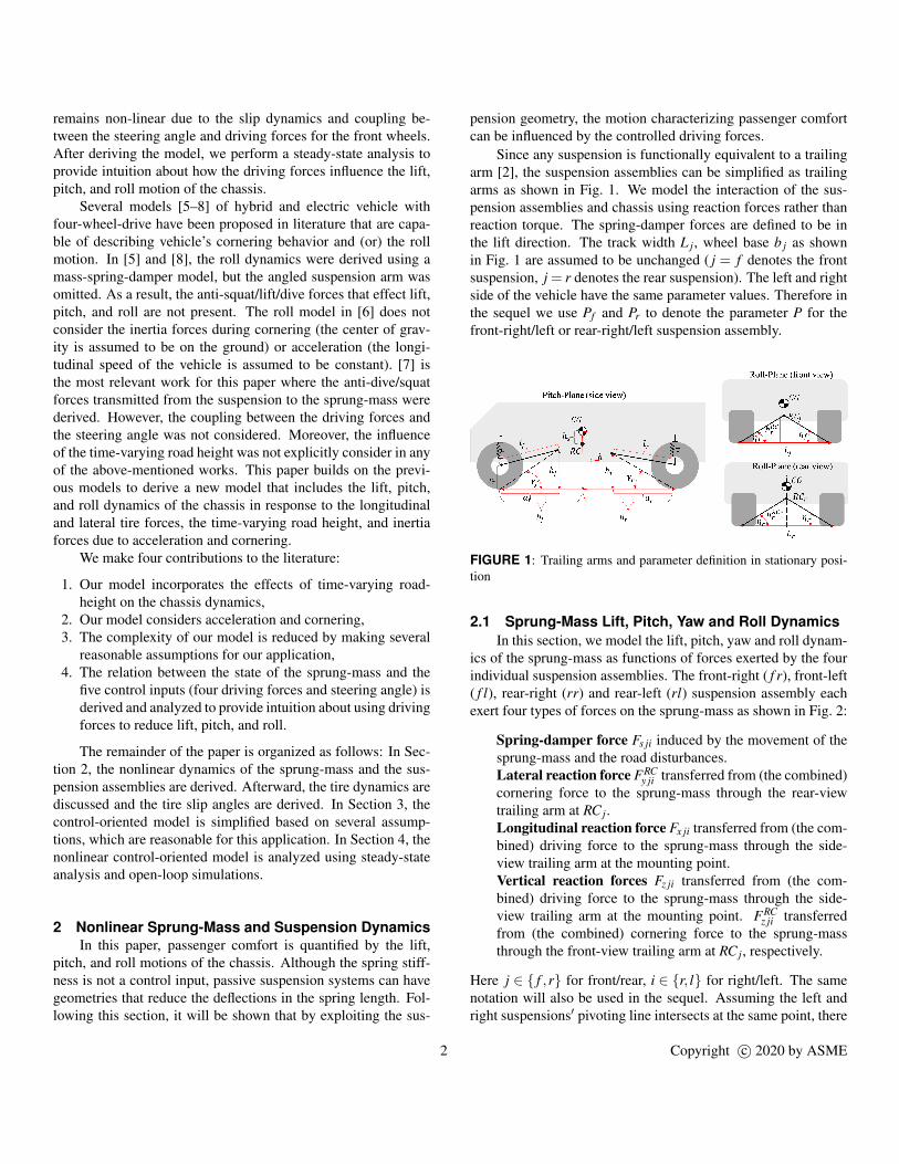
Since any suspension is functionally equivalent to a trailingarm [2], the suspension assemblies can be simplified as trailingarms as shown in Fig. 1. We model the interaction of the sus-pension assemblies and chassis using reaction forces rather thanreaction torque. The spring-damper forces are defined to be inthe lift direction. The track width L j, wheel base b j as shownin Fig. 1 are assumed to be unchanged ( j = f denotes the frontsuspension, j = r denotes the rear suspension). The left and rightside of the vehicle have the same parameter values. Therefore inthe sequel we use Pf and Pr to denote the parameter P for thefront-right/left or rear-right/left suspension assembly.

FIGURE 1: Trailing arms and parameter definition in stationary posi-tion

2.1 Sprung-Mass Lift, Pitch, Yaw and Roll DynamicsIn this section, we model the lift, pitch, yaw and roll dynam-

ics of the sprung-mass as functions of forces exerted by the fourindividual suspension assemblies. The front-right ( f r), front-left( f l), rear-right (rr) and rear-left (rl) suspension assembly eachexert four types of forces on the sprung-mass as shown in Fig. 2:

Spring-damper force Fs ji induced by the movement of thesprung-mass and the road disturbances.Lateral reaction force FRC

y ji transferred from (the combined)cornering force to the sprung-mass through the rear-viewtrailing arm at RC j.Longitudinal reaction force Fx ji transferred from (the com-bined) driving force to the sprung-mass through the side-view trailing arm at the mounting point.Vertical reaction forces Fz ji transferred from (the com-bined) driving force to the sprung-mass through the side-view trailing arm at the mounting point. FRC

z ji transferredfrom (the combined) cornering force to the sprung-massthrough the front-view trailing arm at RC j, respectively.

Here j ∈ { f ,r} for front/rear, i ∈ {r, l} for right/left. The samenotation will also be used in the sequel. Assuming the left andright suspensions′ pivoting line intersects at the same point, there


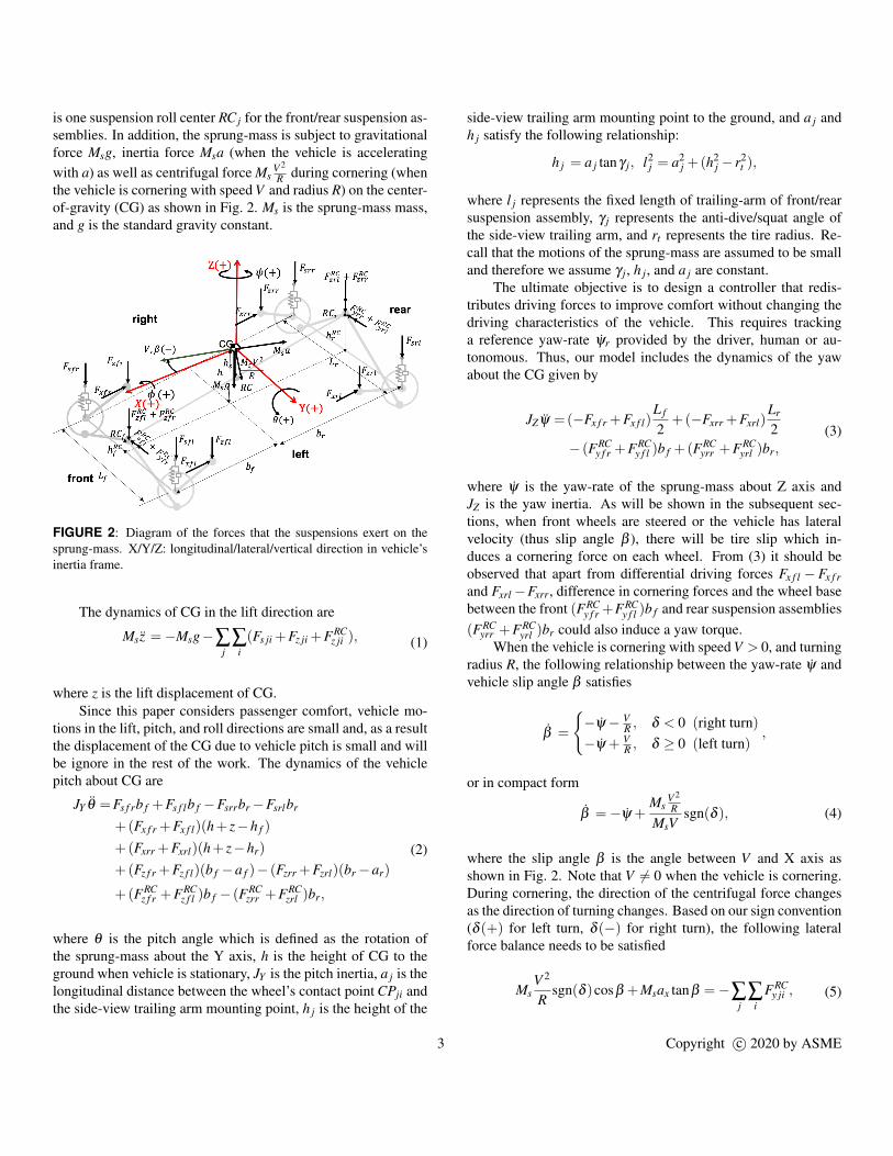
is one suspension roll center RC j for the front/rear suspension as-semblies. In addition, the sprung-mass is subject to gravitationalforce Msg, inertia force Msa (when the vehicle is acceleratingwith a) as well as centrifugal force Ms

V 2

R during cornering (whenthe vehicle is cornering with speed V and radius R) on the center-of-gravity (CG) as shown in Fig. 2. Ms is the sprung-mass mass,and g is the standard gravity constant.

FIGURE 2: Diagram of the forces that the suspensions exert on thesprung-mass. X/Y/Z: longitudinal/lateral/vertical direction in vehicle’sinertia frame.

The dynamics of CG in the lift direction are

Msz =−Msg−∑j∑

i(Fs ji +Fz ji +FRC

z ji ), (1)

where z is the lift displacement of CG.Since this paper considers passenger comfort, vehicle mo-

tions in the lift, pitch, and roll directions are small and, as a resultthe displacement of the CG due to vehicle pitch is small and willbe ignore in the rest of the work. The dynamics of the vehiclepitch about CG are

JY θ =Fs f rb f +Fs f lb f −Fsrrbr−Fsrlbr

+(Fx f r +Fx f l)(h+ z−h f )

+(Fxrr +Fxrl)(h+ z−hr)

+(Fz f r +Fz f l)(b f −a f )− (Fzrr +Fzrl)(br−ar)

+(FRCz f r +FRC

z f l )b f − (FRCzrr +FRC

zrl )br,

(2)

where θ is the pitch angle which is defined as the rotation ofthe sprung-mass about the Y axis, h is the height of CG to theground when vehicle is stationary, JY is the pitch inertia, a j is thelongitudinal distance between the wheel’s contact point CPji andthe side-view trailing arm mounting point, h j is the height of the

side-view trailing arm mounting point to the ground, and a j andh j satisfy the following relationship:

h j = a j tanγ j, l2j = a2

j +(h2j − r2

t ),

where l j represents the fixed length of trailing-arm of front/rearsuspension assembly, γ j represents the anti-dive/squat angle ofthe side-view trailing arm, and rt represents the tire radius. Re-call that the motions of the sprung-mass are assumed to be smalland therefore we assume γ j, h j, and a j are constant.

The ultimate objective is to design a controller that redis-tributes driving forces to improve comfort without changing thedriving characteristics of the vehicle. This requires trackinga reference yaw-rate ψr provided by the driver, human or au-tonomous. Thus, our model includes the dynamics of the yawabout the CG given by

JZψ =(−Fx f r +Fx f l)L f

2+(−Fxrr +Fxrl)

Lr

2− (FRC

y f r +FRCy f l )b f +(FRC

yrr +FRCyrl )br,

(3)

where ψ is the yaw-rate of the sprung-mass about Z axis andJZ is the yaw inertia. As will be shown in the subsequent sec-tions, when front wheels are steered or the vehicle has lateralvelocity (thus slip angle β ), there will be tire slip which in-duces a cornering force on each wheel. From (3) it should beobserved that apart from differential driving forces Fx f l − Fx f rand Fxrl−Fxrr, difference in cornering forces and the wheel basebetween the front (FRC

y f r +FRCy f l )b f and rear suspension assemblies

(FRCyrr +FRC

yrl )br could also induce a yaw torque.When the vehicle is cornering with speed V > 0, and turning

radius R, the following relationship between the yaw-rate ψ andvehicle slip angle β satisfies

β =

{−ψ− V

R , δ < 0 (right turn)−ψ + V

R , δ ≥ 0 (left turn),

or in compact form

β =−ψ +Ms

V 2

RMsV

sgn(δ ), (4)

where the slip angle β is the angle between V and X axis asshown in Fig. 2. Note that V 6= 0 when the vehicle is cornering.During cornering, the direction of the centrifugal force changesas the direction of turning changes. Based on our sign convention(δ (+) for left turn, δ (−) for right turn), the following lateralforce balance needs to be satisfied

MsV 2

Rsgn(δ )cosβ +Msax tanβ =−∑

j∑

iFRC

y ji , (5)


where MsV 2

R cosβ sgn(δ ) and Msax tanβ are the centrifugal forcedue to cornering and the inertia force due to acceleration pro-jected onto the lateral direction, respectively.

To prevent changing the driving characteristics of the vehi-cle, its acceleration ax should match the reference ar

x provided bythe driver, human or autonomous. The longitudinal accelerationax is determined by the force balance in the X-direction

Msax =−∑j∑

iFx ji +Ms

V 2

Rsgn(δ )sinβ .

Note that the longitudinal acceleration ax will also be influencedby centrifugal force Ms

V 2

R if vehicle has lateral velocity and thusslip angle β . With (5), the above equation can be simplified as

Msax =−∑j∑

iFx ji cos2

β −∑j∑

iFRC

y ji sinβ cosβ . (6)

Note that the desired acceleration arx can be achieved ax = ar

x byproper choice of the sum of driving forces ∑ j ∑i Fx ji.

During cornering, the centrifugal force on CG will causeload transfer to one side of the vehicle. As a result, the vehi-cle body will roll around the roll axis, which is obtained by con-necting RC f to RCr as are shown in Fig. 2, and the vehicle body(sprung-mass) rolls around the roll axis. The roll center (RC) asshown in Fig. 2 is the vertical projection of the CG onto roll axiswhen vehicle is in stationary position. Note that although the rollcenter and roll axis may change with vehicle movement, in thesequel they are assume to be constant based on our assumptionthat the lift, yaw and roll motion is small.

For passenger vehicles, the displacement of the CG due tovehicle roll is very small in most cases and can generally be ig-nored [1]. Thus, the dynamics of the vehicle roll around CG aregiven by

JX φ =(Fs f r−Fs f l)L f

2+(Fsrr−Fsrl)

Lr

2

+(Fz f r−Fz f l)L f

2+(Fzrr−Fzrl)

Lr

2− (FRC

y f r +FRCy f l )((h+ z)−hRC

f)

− (FRCyrr +FRC

yrl )((h+ z)−hRC

r),

(7)

where φ is the roll angle of the sprung-mass around X axis andJX is the roll inertia. hRC

j is the RC height of the suspensionassembly.

With (5) and (6), the dynamics of the slip β can be simplifiedas

β =−ψ +∑ j ∑i(Fx ji sinβ −FRC

y ji cosβ )

MsVx, (8)

where Vx = V cosβ is the vehicle longitudinal velocity and itsdynamics are related by

Vx = ax, (9)

where the longitudinal acceleration ax is determined by (6).The state of the sprung-mass is x = [z, z,θ , θ ,φ , φ ,β , ψ]T

where z, z,θ , θ ,φ , φ are included to model performance, β isincluded due to its influence on the roll φ , and ψ is includedto ensure that the driving characteristics of the vehicle are notchanged. From (1), (2), (3) and (7) it can be seen that the dy-namics of the lift, pitch, yaw and roll are linear in terms of thesuspension forces. However, in the following sections, we willshow that the suspension forces are nonlinear functions of thestate x = [z, z,θ , θ ,φ , φ ,β , ψ]T , control inputs, and the road dis-turbances.

2.2 Rear Suspension ForcesIn this section we derive the forces that the rear-right and

rear-left suspension assemblies exert on the sprung-mass. Weassume that the suspension assemblies are at quasi-equilibriumand therefore the forces and torques applied to the suspensionsassemblies are balanced [9]. With only front-wheel steering thereis no coupling between driving forces uri and cornering forcesnri.

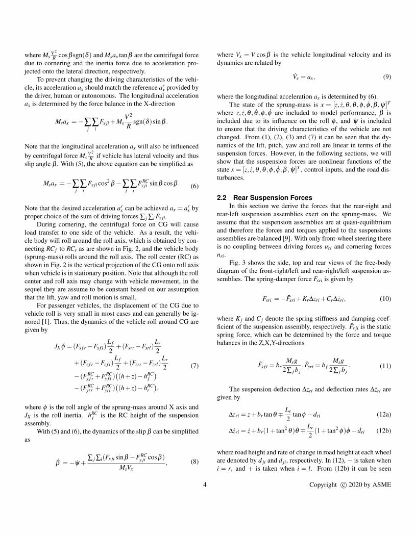
Fig. 3 shows the side, top and rear views of the free-bodydiagram of the front-right/left and rear-right/left suspension as-semblies. The spring-damper force Fsri is given by

Fsri =−Fsri +Kr∆zri +Cr∆zri, (10)

where K j and C j denote the spring stiffness and damping coef-ficient of the suspension assembly, respectively. Fs ji is the staticspring force, which can be determined by the force and torquebalances in the Z,X,Y-directions

Fs f i = brMsg

2∑ j b j, Fsri = b f

Msg2∑ j b j

. (11)

The suspension deflection ∆zri and deflection rates ∆zri aregiven by

∆zri = z+br tanθ ∓ Lr

2tanφ −dri (12a)

∆zri = z+br(1+ tan2θ)θ ∓ Lr

2(1+ tan2

φ)φ − dri (12b)

where road height and rate of change in road height at each wheelare denoted by d ji and d ji, respectively. In (12), − is taken wheni = r, and + is taken when i = l. From (12b) it can be seen


FIGURE 3: Free-body diagram of the front and rear suspension assemblies

that the suspension deflection rates are nonlinear functions of thestate of the sprung-mass. As a result, the spring-damper forces(10) are nonlinear functions of the state of the sprung-mass.

The force balance in the X-direction and torque balancearound tire contact point CPri (see the side view in Fig. 3) yieldthe following relationships

Fxri =−uri (13a)Fzri =−uri tanγr. (13b)

It can be seen from (13) that the reaction forces in the side vieware functions of driving forces. In particular, the force (13b) pro-vides control authority over the lift (1), pitch (2), and roll (7)dynamics. Note that lift reaction force Fzri in (13b) is negativewhen uri > 0 during acceleration, per Newton’s third law the liftreaction force that the suspension assembly exerts on the sprung-mass is positive. Thus, the suspension produces an anti-squatreaction force during acceleration and hence this type of suspen-sion is called anti-squat suspension. Similar effects also appearsin the front suspension design (anti-dive).

The force balance in the Y-direction and torque balancearound tire contact point CPri yield the following expressions forthe roll forces

FRCyri = nri, (14a)

FRCzri =±nri tanηr. (14b)

where η j denotes the angle between the trailing arm and theground in the rear view. In (14b), + is taken when i = r, − istaken when i = l. Recall that η j is assumed to be constant sincethe vehicle motions are small.

It can be seen from (14) that the reaction forces in the rearview are functions of cornering forces nri. Note that from (14b),

a vertical reaction force will be induced by the cornering force.This explains the source of ”jacking” forces inherent to indepen-dent suspensions [2]. If the cornering force on the right-sidewheel nrr and the left-side wheel nrl has same magnitude, thedownward vertical reaction force induced by the cornering forceon one wheel will cancel out the lifting effect from the otherwheel due to its induced upward vertical reaction force.

The combined driving force uri and cornering force nri cannot exceed the tire friction limit µ jiN ji, where µ ji and N ji are thefriction coefficient and normal force on each tire, respectively.The normal forces on the rear-right/left suspension assembly canbe expressed as

Nri =Mrig−Fsri−Fzri−FRCzri , (15)

where Mri is the wheel mass of the rear-right/left wheel.

2.3 Front Suspension ForcesThe forces produced by the front suspension assemblies dif-

fer from the rear due to the steering angle. Since the two frontwheels are used for both driving and steering, the longitudinaland lateral forces on the front wheels depend on both the steer-ing angle δi and the driving force u f i (see the top view in Fig. 3)

Fcbx f i = u f i cosδi +n f i sinδi (16a)

Fcby f i =−u f i sinδi +n f i cosδi, (16b)

where Fcbx f i and Fcb

y f i denote the combined forces in the X and Y-direction, respectively.

With the combined forces (16) in the X (16a) and Y-direction(16b), the modeling of the front suspension assemblies are simi-lar to that of the rear suspension assemblies in the previous sec-tion. Similar to (10) and (12), the spring-damper force Fs f i, the


suspension deflection ∆z f i, as well as the deflection rate ∆z f i aregiven by

Fs f i =−Fs f i +K f ∆z f i +C f ∆z f i (17)

∆z f i = z−b f tanθ ∓L f

2tanφ −d f i (18a)

∆z f i = z−b f (1+ tan2θ)θ ∓

L f

2(1+ tan2

φ)φ − d f i, (18b)

where the static spring force Fs f i is given in (11). In (18), − istaken when i = r, + is taken when i = l.

Unlike the rear suspension assemblies, the reaction forces inthe side and rear views are now induced by the combined drivingand cornering forces. The force and torque balance (see the sideand rear view in Fig. 3) yield the following relationships In theside-view,

Fx f i =−Fcbx f i, (19a)

Fz f r = Fcbx f i tanγ f . (19b)

In the rear-view,

FRCy f i = Fcb

y f i, (20a)

FRCz f i =±Fcb

y f i tanη f . (20b)

In (20b), + is taken when i = r, − is taken when i = l.Again, the combined driving force u f i and cornering force

n f i are limited by the normal force N f i on each tire. The normalforce on the suspension assembly can be expressed according tothe force balance in the Z direction

N f i =M f ig−Fs f i−Fz f i−FRCz f i , (21)

where M f i is the wheel mass of the front-right/left wheel.

2.4 Linear tire model and cornering forcesSince the vehicle considered is operating under normal driv-

ing conditions, a linear model of tire forces is used

n ji =Cαj α ji, (22)

where Cαj is the cornering stiffness of the front/rear tires. The

tire slip angle α ji is the angle between the wheel’s velocity vec-tor along the wheel center plane and the vehicle’s actual direc-tion of displacement at the tire contact patch [1]. It can be ob-

tained through the rigid body motion and the velocity vector cor-responding to each tire [3]

V cosβ

V sinβ

0

+0

0ψ

× b f

∓L f2

0

=

Vf i cos(δi +α f i)Vf i sin(δi +α f i)

0

(23a)

V cosβiV sinβi

0

+0

0ψ

×−br

∓Lr2

0

=

Vri cosαriVri sinαri

0

, (23b)

where Vji is the speed at the tire contact point of each wheel. In(23), − is taken when i = r, + is taken when i = l. The firsttwo components in the vector equations (23a) and (23b) offerthe relationship among the slip angle, the steering angle and thevehicle slip angle:

tan(δi +α f i) =V sinβ + ψb f

V cosβ ± ψL f2

, tanαri =V sinβ − ψbr

V cosβ ± ψLr2

,

where + is taken when i = r, − is taken when i = l. The aboveequation leads to the following tire slip angles expressions:

α f i = arctan

(V sinβ + ψb f

V cosβ ± ψL f2

)−δi (24a)

αri = arctan

(V sinβ − ψbr

V cosβ ± ψLr2

), (24b)

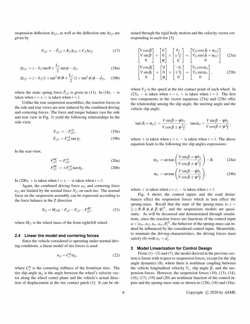
where + is taken when i = r, − is taken when i = l.Fig. 4 shows the control inputs and the road distur-

bances effect the suspension forces which in turn effect thesprung-mass. Recall that the state of the sprung-mass is x =[z, z,θ , θ ,φ , φ ,β , ψ]T , and the suspensions models are quasi-static. As will be discussed and demonstrated through simula-tions, since the reaction forces are functions of the control inputu = [u f r,u f l ,urr,url ,δ ]

T , the behavior of the sprung-mass can in-deed be influenced by the considered control input. Meanwhile,to maintain the driving-characteristics, the driving forces mustsatisfy (6) with ax = ar

x.

3 Model Linearization for Control DesignFrom (1)−(3) and (7), the model derived in the previous sec-

tion is linear with respect to suspension forces, except for the slipangle dynamics (8), where there is nonlinear coupling betweenthe vehicle longitudinal velocity Vx, slip angle β , and the sus-pension forces. However, the suspension forces (10), (13), (14),(16), (17), (19) and (20) are nonlinear function of the control in-puts and the sprung-mass state as shown in (12b), (16) and (18a).


Fs f i (17)

Fx f i (19a)

Fz f i (20a)

FRCy f i (19b)

FRCz f i (20b)

Fsri (10)

Fxri (13a)

Fzri (13b)

FRCyri (14a)

FRCzri (14b)

x, Vx (9)

Lift z (1)

Pitch θ (2)

Roll φ (7)

Slip angle β (8)

Yaw-rate ψ (3)

FIGURE 4: Model diagram of the suspension assemblies and thesprung-mass as a dynamic system.

Consequently the relationship from the control inputs and theroad disturbances to the sprung-mass state as shown in Fig. 4 iscomplicated. In addition, the tire slip angles in (24) have nonlin-ear expressions. For the control design, a simplified model maysuffice based on several reasonable assumptions.

3.1 Assumptions for simplificationTo simplify the model, we make the following assumptions

since the vehicle is under normal driving condition

A.1 Small angle assumption: sin · ≈ tan · ≈ ·, and cos · ≈ 1.A.2 The steering angles are the same for the front left and right

wheels: δr = δl = δ .A.3 The lift motion z is small compared to the height of CG h

(z� h): h+ z≈ h.A.4 The longitudinal velocity is larger compared to the velocity

induced by yaw-rate in the longitudinal direction (V cosβ �ψ

L f2 , V cosβ � ψ

Lr2 ): V cosβ ± ψ

L f2 ≈ V cosβ ± ψ

Lr2 ≈

V cosβ .A.5 The lateral velocity Vy of the vehicle is small: Vx ≈V .

Based on A.1, A.2, A.4 and A.5, the slip angle of each tirecan be simplified from (24) as

α f i ≈ β +ψb f

Vx−δ , αri ≈ β − ψbr

Vx. (25)

Based on A.1, A.2, A.5 and (25), the relationship betweenax and u, x can be simplified as

Msax ≈∑u ji +∑u f iδβ −2Cαr (β −

br

Vxψ)β

+2Cαf (β +

b f

Vxψ−δ )(δ −β ),

(26)

where there are no dynamics in ax. In other words, (26) is anequality constraint on the driving forces ui j.

In addition, based on A.1 and (25), the normal forces on therear-right/left wheel (15) is simplified as

Nri ≈Mrig+ Fsri−Kr(z+brθ ∓Lr

2φ −dri)

−Cr(z+brθ ∓Lr

2φ − dri)+ tanγruri

∓Cαr (β −

br

Vxψ) tanηr,

(27)

where− is taken when i= r, and + is taken when i= l. Likewise,the normal forces on the front-right/left wheel (21) is simplifiedas

N f i ≈M f ig+ Fs f i−K f (z−b f θ ∓L f

2φ −d f i)

−C f (z−b f θ ∓L f

2φ − d f i)

− tanγ f (u f i +Cαf (β +

b f

Vxψ−δ )δ )

∓ (−u f iδ +Cαf (β +

b f

Vxψ−δ )) tanη f ,

(28)

where − is taken when i = r, and + is taken when i = l.Based on the above assumptions and linearized expression

of tire slip angles (25), the model derived in Section 2 can besimplified for control design. To summarize, the control-orientedmodel can be written as

x = f (x,u,d,Vx) , (29)

where d = [d f r, d f r,d f l , d f l ,drr, drr,drl , drl ]T . Detailed equations

of (29) are omitted here due to space limitation, but can be easilyderived from the nonlinear model with the above assumptionsA.1-A.5 and the tire slip angles (25).

3.2 Local Controllability of the Control-OrientedModel

The symbolic Jacobian matrices of (29) can be obtained withMatlab Symbolic Math Toolbox:

A :=∂ f∂x

= A(x,u,Vx) (30a)

Bu :=∂ f∂u

= Bu (x,u,Vx) , (30b)

where the linearized state-space matrices A and B depend in-versely 1

Vxon the longitudinal velocity. The symbolic control-

lability matrix [Bu,ABu, ...,A7Bu] has full rank irrespective of


the choice of operating conditions (Vx 6= 0). Consequently, thenonlinear system (29) is locally controllable at any equilibriumpoint through the sufficient condition for local controllability atan equilibrium point [4].

4 Open-Loop SimulationsIn this section, we analyze how the control inputs influence

the sprung-mass motion using the linearized model (30) witha constant driving speed ax = 0 and Vx 6= 0. Afterwards, weshow that passenger comfort can indeed be influenced by thecontrol inputs using open-loop step responses of both the non-linear (Fig. 4) and linearized (30) models. In addition, these stepresponses validate our linearization and steady-state analysis.

Note that in the open-loop simulation, the actual acceler-ation is obtained from (6). Thus, the control input does notguarantee ax = ar

x = 0. Consequently, the actual velocity mightchange as time evolves within each simulation. System parame-ters used in this work are summarized in Table 1.

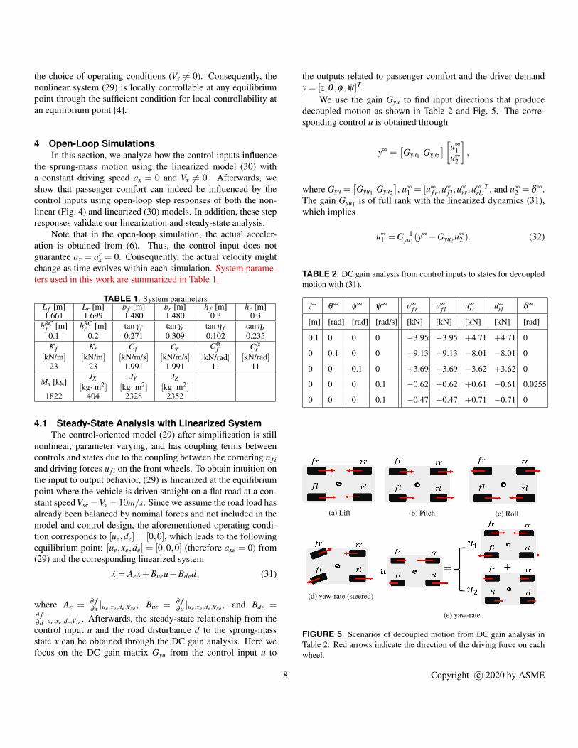
TABLE 1: System parametersL f [m] Lr [m] b f [m] br [m] h f [m] hr [m]1.661 1.699 1.480 1.480 0.3 0.3

hRCf [m] hRC

r [m] tanγ f tanγr tanη f tanηr0.1 0.2 0.271 0.309 0.102 0.235K f

[kN/m]Kr

[kN/m]C f

[kN/m/s]Cr

[kN/m/s]Cα

f[kN/rad]

Cαr

[kN/rad]23 23 1.991 1.991 11 11

Ms [kg]JX

[kg· m2]JY

[kg· m2]JZ

[kg· m2]1822 404 2328 2352

4.1 Steady-State Analysis with Linearized SystemThe control-oriented model (29) after simplification is still

nonlinear, parameter varying, and has coupling terms betweencontrols and states due to the coupling between the cornering n f iand driving forces u f i on the front wheels. To obtain intuition onthe input to output behavior, (29) is linearized at the equilibriumpoint where the vehicle is driven straight on a flat road at a con-stant speed Vxe =Ve = 10m/s. Since we assume the road load hasalready been balanced by nominal forces and not included in themodel and control design, the aforementioned operating condi-tion corresponds to [ue,de] = [0,0], which leads to the followingequilibrium point: [ue,xe,de] = [0,0,0] (therefore axe = 0) from(29) and the corresponding linearized system

x = Aex+Bueu+Bded, (31)

where Ae = ∂ f∂x |ue,xe,de,Vxe , Bue = ∂ f

∂u |ue,xe,de,Vxe , and Bde =∂ f∂d |ue,xe,de,Vxe . Afterwards, the steady-state relationship from thecontrol input u and the road disturbance d to the sprung-massstate x can be obtained through the DC gain analysis. Here wefocus on the DC gain matrix Gyu from the control input u to

the outputs related to passenger comfort and the driver demandy = [z,θ ,φ , ψ]T .

We use the gain Gyu to find input directions that producedecoupled motion as shown in Table 2 and Fig. 5. The corre-sponding control u is obtained through

y∞ =[Gyu1 Gyu2

][u∞1

u∞2

],

where Gyu =[Gyu1 Gyu2

], u∞

1 = [u∞f r,u

∞f l ,u

∞rr,u

∞rl ]

T , and u∞2 = δ ∞.

The gain Gyu1 is of full rank with the linearized dynamics (31),which implies

u∞1 =G−1

yu1(y∞−Gyu2u∞

2 ). (32)

TABLE 2: DC gain analysis from control inputs to states for decoupledmotion with (31).

z∞ θ ∞ φ ∞ ψ∞ u∞f r u∞

f l u∞rr u∞

rl δ ∞

[m] [rad] [rad] [rad/s] [kN] [kN] [kN] [kN] [rad]

0.1 0 0 0 −3.95 −3.95 +4.71 +4.71 0

0 0.1 0 0 −9.13 −9.13 −8.01 −8.01 0

0 0 0.1 0 +3.69 −3.69 −3.62 +3.62 0

0 0 0 0.1 −0.62 +0.62 +0.61 −0.61 0.0255

0 0 0 0.1 −0.47 +0.47 +0.71 −0.71 0

(a) Lift (b) Pitch (c) Roll

(d) yaw-rate (steered)

(e) yaw-rate

FIGURE 5: Scenarios of decoupled motion from DC gain analysis inTable 2. Red arrows indicate the direction of the driving force on eachwheel.


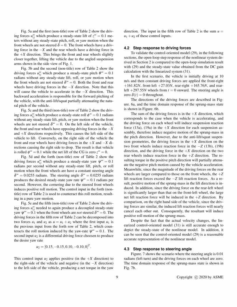
Fig. 5a and the first (non-title) row of Table 2 show the driv-ing forces u∞

i j which produce a steady-state lift of z∞ = 0.1 me-ters without any steady-state pitch, roll, or yaw motion when thefront wheels are not steered δ = 0. The front wheels have a driv-ing force in the −X and the rear wheels have a driving force inthe +X direction. This brings the front and rear wheels slightlycloser together, lifting the vehicle due to the angled suspensionarms shown in the side view of Fig. 1.

Fig. 5b and the second (non-title) row of Table 2 show thedriving forces u∞

i j which produce a steady-state pitch θ ∞ = 0.1radians without any steady-state lift, roll, or yaw motion whenthe front wheels are not steered δ ∞ = 0. Both the front and rearwheels have driving forces in the −X direction. Note that thiswill cause the vehicle to accelerate in the −X direction. Thisbackward acceleration is responsible for the forward pitching ofthe vehicle, with the anti-lift/squat partially attenuating the natu-ral pitch of the vehicle.

Fig. 5c and the third (non-title) row of Table 2 show the driv-ing forces u∞

i j which produce a steady-state roll φ ∞ = 0.1 radianswithout any steady-state lift, pitch, or yaw motion when the frontwheels are not steered δ ∞ = 0. On the left side of the vehicle,the front and rear wheels have opposing driving forces in the−Xand +X directions respectively. This causes the left side of thevehicle to lift. Conversely, on the right side of the vehicle thefront and rear wheels have driving forces in the +X and −X di-rections causing the right side to drop. The result is that vehicleis rolled φ ∞ = 0.1 while the net lift of the CG is zero z∞ = 0.

Fig. 5d and the forth (non-title) row of Table 2 show thedriving forces u∞

i j which produce a steady-state yaw ψ∞ = 0.1radians per second without any steady-state lift, pitch, or rollmotion when the front wheels are have a constant steering angleδ ∞ = 0.0255 radians. The steering angle δ ∞ = 0.0255 radiansproduces the desired steady-state yaw rate ψ∞ = 0.1 radians persecond. However, the cornering due to the steered front wheelsinduces positive roll motion. The control input in the forth (non-title) row of Table 2 is used to counteract this roll motion, result-ing in a pure yaw-motion.

Fig. 5e and the fifth (non-title) row of Table 2 show the driv-ing forces u∞

i j needed to again produce a decoupled steady-stateyaw ψ∞ = 0.1 when the front wheels are not steered δ ∞ = 0. Thedriving forces in the fifth row of Table 2 can be decomposed intotwo forces u1 and u2 as u = u1 + u2 where the first input u1 isthe previous input from the forth row of Table 2, which coun-teracts the roll motion induced by the yaw-rate ψ∞ = 0.1. Thesecond input u2 is a differential driving force choosen to producethe desire yaw rate

u2 = [0.15,−0.15,0.10,−0.10,0]T .

This control input u2 applies positive (in the +X direction) tothe right-side of the vehicle and negative (in the −X direction)to the left-side of the vehicle, producing a net torque in the yaw

direction. The input in the fifth row of Table 2 is the sum u =u1 +u2 of these control inputs.

4.2 Step response to driving forcesTo validate the control-oriented model (29), in the following

sections, the open-loop step response of the nonlinear system de-rived in Section 2 is compared to the open-loop simulation resultwith (29) and the steady-state value obtained from the DC gaincalculation with the linearized system (31).

In the first scenario, the vehicle is initially driving at 10m/s and then constant driving forces are applied the front-right+161.82N, front-left +27.03N, rear-right +165.76N, and rear-left +297.55N wheels from t = 0 onward. The steering angle iszero δ (t) = 0 throughout.

The directions of the driving forces are described in Fig-ure. 6a, and the time domain response of the sprung-mass stateis shown in Figure. 6b.

The sum of the driving forces is in the +X direction, whichcorresponds to the case when the vehicle is accelerating, andthe driving force on each wheel will induce suspension reactionforce (13a), (19a) in the +X direction for each suspension as-sembly, therefore induce negative motion of the sprung-mass inthe pitch direction. However, due to the anti-lift/squat suspen-sion geometries, the driving forces in the +X direction on thetwo front wheels induce reaction force in the −Z (13b), (19b)direction, and the driving force in the +X direction on the tworear wheels induce reaction force in the +Z direction. The re-sulting torque in the positive pitch direction will partially attenu-ate the negative pitch motion caused by the vehicle acceleration.Meanwhile, since the magnitude of the driving forces on the rearwheels are larger compared to those on the front wheels, the +Zlift reaction forces exceed the −Z lift reaction forces. As a re-sult, positive motion of the sprung-mass in the lift direction is in-duced. In addition, since the driving force on the rear-left wheelis significantly larger than that on the front-left wheel, the largenet lift reaction force will be induced in the +Z direction. Bycomparison, on the right hand side of the vehicle, since the driv-ing forces are similar, the induced lift reaction forces will nearlycancel each other out. Consequently, the resultant will inducepositive roll motion of the sprung-mass.

Despite the fact that the actual velocity changes, the lin-earized control-oriented model (31) is still accurate enough todepict the steady-state of the nonlinear model. In addition, itcan be seen that the control-oriented model (29) is a reasonableaccurate representation of the nonlinear model.

4.3 Step response to steering angleFigure. 7 shows the scenario where the steering angle is 0.01

radians (left turn) and the driving forces on each wheel are zero.The time domain response of the sprung-mass state is shown inFig. 7b.


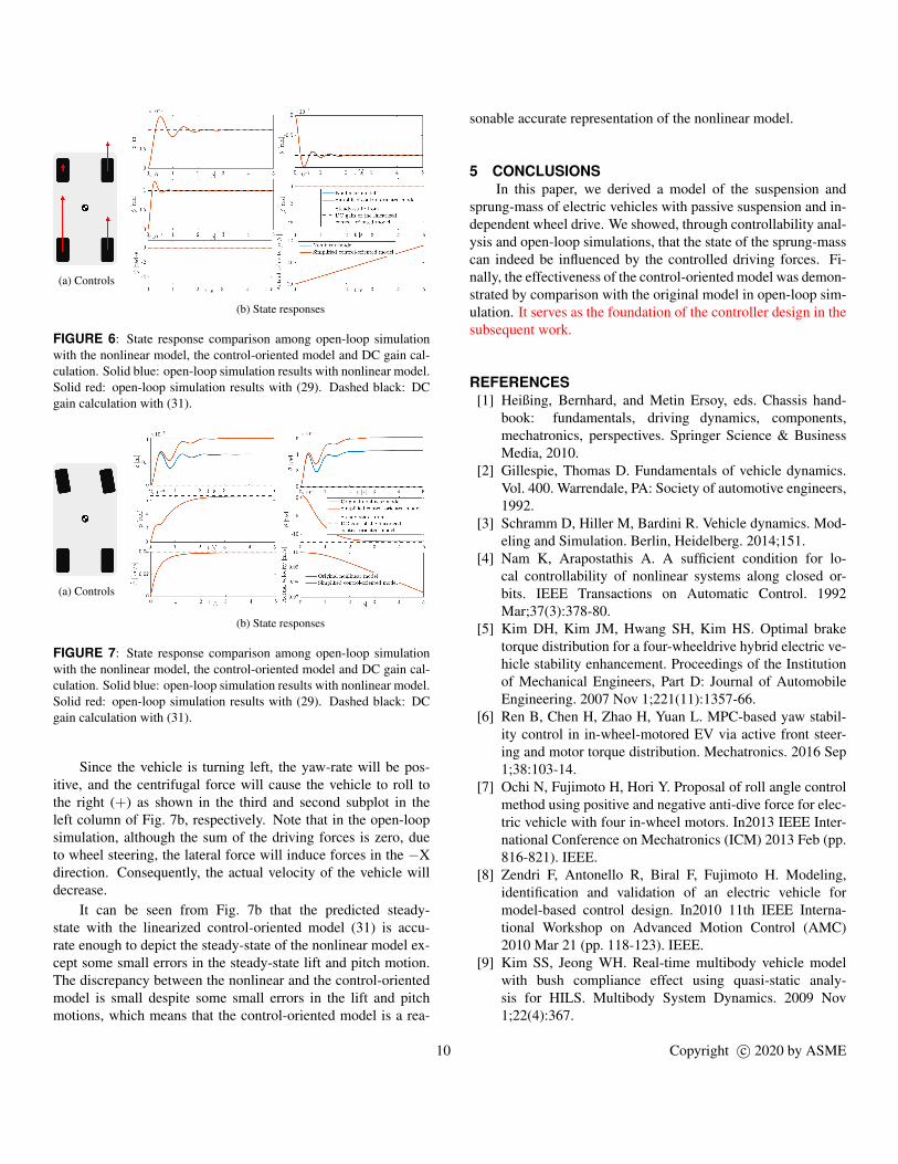
(a) Controls

(b) State responses

FIGURE 6: State response comparison among open-loop simulationwith the nonlinear model, the control-oriented model and DC gain cal-culation. Solid blue: open-loop simulation results with nonlinear model.Solid red: open-loop simulation results with (29). Dashed black: DCgain calculation with (31).

(a) Controls

(b) State responses

FIGURE 7: State response comparison among open-loop simulationwith the nonlinear model, the control-oriented model and DC gain cal-culation. Solid blue: open-loop simulation results with nonlinear model.Solid red: open-loop simulation results with (29). Dashed black: DCgain calculation with (31).

Since the vehicle is turning left, the yaw-rate will be pos-itive, and the centrifugal force will cause the vehicle to roll tothe right (+) as shown in the third and second subplot in theleft column of Fig. 7b, respectively. Note that in the open-loopsimulation, although the sum of the driving forces is zero, dueto wheel steering, the lateral force will induce forces in the −Xdirection. Consequently, the actual velocity of the vehicle willdecrease.

It can be seen from Fig. 7b that the predicted steady-state with the linearized control-oriented model (31) is accu-rate enough to depict the steady-state of the nonlinear model ex-cept some small errors in the steady-state lift and pitch motion.The discrepancy between the nonlinear and the control-orientedmodel is small despite some small errors in the lift and pitchmotions, which means that the control-oriented model is a rea-

sonable accurate representation of the nonlinear model.

5 CONCLUSIONSIn this paper, we derived a model of the suspension and

sprung-mass of electric vehicles with passive suspension and in-dependent wheel drive. We showed, through controllability anal-ysis and open-loop simulations, that the state of the sprung-masscan indeed be influenced by the controlled driving forces. Fi-nally, the effectiveness of the control-oriented model was demon-strated by comparison with the original model in open-loop sim-ulation. It serves as the foundation of the controller design in thesubsequent work.

REFERENCES[1] Heißing, Bernhard, and Metin Ersoy, eds. Chassis hand-

book: fundamentals, driving dynamics, components,mechatronics, perspectives. Springer Science & BusinessMedia, 2010.

[2] Gillespie, Thomas D. Fundamentals of vehicle dynamics.Vol. 400. Warrendale, PA: Society of automotive engineers,1992.

[3] Schramm D, Hiller M, Bardini R. Vehicle dynamics. Mod-eling and Simulation. Berlin, Heidelberg. 2014;151.

[4] Nam K, Arapostathis A. A sufficient condition for lo-cal controllability of nonlinear systems along closed or-bits. IEEE Transactions on Automatic Control. 1992Mar;37(3):378-80.

[5] Kim DH, Kim JM, Hwang SH, Kim HS. Optimal braketorque distribution for a four-wheeldrive hybrid electric ve-hicle stability enhancement. Proceedings of the Institutionof Mechanical Engineers, Part D: Journal of AutomobileEngineering. 2007 Nov 1;221(11):1357-66.

[6] Ren B, Chen H, Zhao H, Yuan L. MPC-based yaw stabil-ity control in in-wheel-motored EV via active front steer-ing and motor torque distribution. Mechatronics. 2016 Sep1;38:103-14.

[7] Ochi N, Fujimoto H, Hori Y. Proposal of roll angle controlmethod using positive and negative anti-dive force for elec-tric vehicle with four in-wheel motors. In2013 IEEE Inter-national Conference on Mechatronics (ICM) 2013 Feb (pp.816-821). IEEE.

[8] Zendri F, Antonello R, Biral F, Fujimoto H. Modeling,identification and validation of an electric vehicle formodel-based control design. In2010 11th IEEE Interna-tional Workshop on Advanced Motion Control (AMC)2010 Mar 21 (pp. 118-123). IEEE.

[9] Kim SS, Jeong WH. Real-time multibody vehicle modelwith bush compliance effect using quasi-static analy-sis for HILS. Multibody System Dynamics. 2009 Nov1;22(4):367.


Suspension Modeling /Author=Chen, Di; Danielson, Clau

Documents

Transcript of Suspension Modeling /Author=Chen, Di; Danielson, Clau