Local Systems and Derived Algebraic Geometry

Harrison Chen

March 10, 2015

Contents

1 Classical notions of local systems 1

2 The stack BG (as a moduli space in algebraic geometry) 3

3 The moduli stack of local systems 6

4 Derived algebraic geometry 9

Introduction

First, a warning. What we call the moduli stack of local systems in this note LocGpXq is called the moduli stack

of G-bundles BunGpXq in the literature, e.g. in [AG:Sing]. In this paper the two notions coincide since for us X

will always be a topological space realized as a locally constant higher stack. However in general one may take X

to be, say, a scheme, which contains “infinitesimal data” to which Loc is sensitive to but Bun is not.

A note on references: Preygel’s note [Pr:Stacks] was very useful for me in understanding the formalism surround-

ing (higher) stacks. Some definitions and discussions can be found in [AG:Sing] and [BN:Loop]. Some statements

and examples were found on MathOverflow. Some additions are due to comments from audience members during

the talk and conversations with David Nadler. For a survey on derived algebraic geometry, see [To:DAG]. These

notes were written with a faulty memory and very incomplete understanding on my part. I expect there will be

errors, and corrections are appreciated.

1 Classical notions of local systems

Definition 1 (A GLn-local system on a space). Let X be a topological space. There are three things which one

might mean by a local system:

(a) [“Betti” definition] a vector bundle π : E Ñ X with parallel transport, i.e. for each homotopy class of paths in

X, a vector space isomorphism between fibers, respecting composition

(b) [“deRahm definition”] if X is a differentiable manifold, a vector bundle π : E Ñ X with a flat connection, i.e. a

map of bundles ∇ : E Ñ E b T˚X satisfying the Leibniz rule ∇ and such that r∇Y ,∇Zs “ 0 for vector fields Y,Z

(one can also write ∇ : TX Ñ EndXpEq)

(c) [sheaf definition] a locally constant sheaf of vector spaces on X

Sketch proof. Definition (a) implies (b) by defining ∇Y at a point x P X as follows: choose a path γ starting at x with

tangent vector given by Y and choose a local trivialization; differentiating the isomorphism gives an endomorphism

of the fiber. Definition (b) implies (c) by locally solving the differential equations and gluing. Definition (c) implies

(a) by the “expand and contract opens” argument: by compactness of r0, 1s, a path in X can be covered by finitely

many opens on which the sheaf is constant. Then, choosing points sequentially in the intersection, one gets a

“zig-zag” of isomorphisms from γp0q to γp1q.

Remark 2. The equivalences (b) and (c) are essentially a special case of the Riemann-Hilbert correspondence.

The full Riemann-Hilbert generalizes (b) to D-modules and (c) to constuctible sheaves.

1

Example 3 (Local systems on the circle). Let X “ S1. Fix a vector space V and assign it to every point. Choose

a point x P X. For every other point in y P X, choose once and for all a path γy : xÑ y and take the identity map

V Ñ V to correspond to this path. Further, choose once and for all a path α : x Ñ x that goes around the circle

once. Every path in S1 from xÑ y is homotopy equivalent to the composition of some number of γ (or its inverse)

and γy. Thus, to give a local system is to give an endomorphism corresponding to γ, i.e. an element of GLpV q.

Note that this is equivalent to giving a map of groups π1pS1q “ ZÑ GLpV q.

Definition 4 (Group-y definition). Let X be a topological space. There are three things which one might mean

by a G-local system:

(a) a principal G-bundle on X with parallel transport, i.e. for each homotopy class of paths in X, an isomorphism

of fibers which is G-equivariant, respecting composition

(b) if X is a differentiable manifold, a principal G-bundle π : E Ñ X with a flat connection, i.e. a map of Lie

algebroids ∇ : TX Ñ e such that r∇X ,∇Y s “ 0 (where e is the associated Lie algebroid to the bundle E; note that

the Leibniz rule translates into the Jacobi identity on TX)

(c) a locally constant sheaf of sets on which the constant sheaf G acts transitively over X

Proof of equivalence for GLn. The following gives a functorial correspondence between vector bundles andG “ GLnbundles. Let V be the standard representation of GLn; to a GLn-torsor P we can associate the vector bundle

P ˆGLn V using the Borel construction. In the other direction, for a vector bundle E over X, one takes the frame

bundle or the trivialization bundle. Parallel transport follows by functoriality.

Remark 5 (Groups other than GLn). Note that for groups other than GLn, the above correspondence is not as

obvious. In general, one could proceed by finding a faithful representation V of G and atempt to define an inverse

functor to the Borel construction functor P ÞÑ P ˆG V . To do so, we need to furnish V with extra structure so

that we can describe G Ă GLpV q.

For example, G “ SLn torsors correspond to vector bundles with the extra data of a trivialization of their top

exterior powers (their determinant bundles). That is, the inverse functor takes a rank n vector bundle E Ñ X with

determinant det : ΛnE » C ˆX and associates to it its torsor of linear automorphisms whose top exterior power

is the identity under det. For G “ SOn, the vector bundles should be equipped with the extra data of an inner

product.

For G semisimple and adjoint type (i.e. with trivial center, e.g. PGL2), the adjoint representation is faithful,

so one can form P ˆG g. We need to have some extra data on this resulting vector bundle in order to recover the

group G as well as the bundle P . It suffices to remember the inner product given by the Killing form, as well as

the Lie bracket. In particular, with this structure we can choose any root datum and thus obtain a map of groups

Autpgq Ñ AutpDq where D is the corresponding Dynkin diagram (note that we need to know the Lie bracket to

talk about Aut and the Killing form to identify root data), and we can recover G as the kernel of this map.

Remark 6 (Alternative: Tannkian correspondence). One can also see this correspondence in a somewhat formal

way. Given a G-bundle P on X, we associate to it a symmetric monoidal functor

ReppGq “ QCohpBGq Ñ QCohpXq

given by the same construction, i.e. V ÞÑ P ˆG V . Then one has defines a local system to be such a functor which

is continuous, right t-exact, and sends flat objects to flat objects. See [AG:Sing] section 10.2 for details.

Remark 7. Finally, we observe that one can write the definition of a G-local system more invariantly by

MappΠ1pXq, BGq

By writing this I mean, for each point of X, assign a set with a G-action, and for each path, a map of such sets

intertwining the action. In particular, for each loop, one gets an automorphism of the G-torsor over a point, i.e. an

element of G.

2

2 The stack BG (as a moduli space in algebraic geometry)

Remark 8 (Functor of points). The Yoneda lemma gives an embedding

X ÞÑ hX “ HomSchp´, Xq : SchopÑ FunpSch,Setq

In other words, knowing a scheme X is the same as knowing all maps from all schemes into X. There is a

problem, however, of characterizing functors Sch Ñ Set which are representable by schemes X which is not easy

in generality. Often moduli problems are more easily stated this way, and objects can also be more easily written

in a coordinate-free way, at the cost of being less explicit. This is the approach we will take in these notes.

Example 9. The functor ΓpXq :“ ΓpX,OXq (i.e. takes global sections) is a sheaf of sets and is represented by a

A1. The functor ΓˆpXq “ ΓpX,OXqˆ is represented by Gm.

Definition 10. A (1-)stack is a (lax 2-)functor1

X : AffopÑ Grpd

satisfying some kind of (etale, fppf) sheaf condition. Note that this is not a higher analogue of schemes but rather

“sheaves of sets.”

Remark 11 (2-categories). The category of groupoids Grpd is a 2-category, which one has to define appropriately.

Whatever it is, it should be the full subcategory of the 2-category of categories Cat consisting of groupoids, i.e.

categories whose morphisms are all invertible. More elaborately, I will just say2 that this 2-category has objects

which are groupoids, (1-)morphisms which are functors between them, and “2-morphisms” between 1-morphisms

which are natural transformations. As one might be used to in category theory, the “correct” notion of equvalence

is not for functors to have inverses on the nose but inverses “up to homotopy” by a natural isomorphism i.e. the

usual notion of equivalence of categories.

We should then also define a functor of 2-categories appropriately, i.e. given a map S1 Ñ S one needs a pullback

map of groupoids XpSq Ñ XpS1q. Here what we mean by lax 2-functor is that Xpgq ˝Xpfq and Xpg ˝ fq need not

be equal but naturally isomorphic.

Remark 12 (Sheaf property). The sheaf property of a functor is with respect to a choice of covers on the source

category (e.g. of schemes), called a Grothendieck topology. Popular candidates are the Zariski (Zariski opens), etale,

or fppf topologies3. I want to surpress this theory for the entire talk, opting instead to just say “locally.” The

easiest example to keep in mind is the Zariski topology, i.e. U is a disjoint union of opens covering X, and U Ñ X

is the obvious map.

A nice formal way to write down the sheaf property for a functor F is to say that a certain truncated simplicial

diagram is limit diagram. However, this notion of limit must be consider in a proper higher categorical way. The

“top” level of the simplicial diagram should be thought of as a condition that must be satisfied, while the other

levels contain data that must be furnished.

Let us do an example of a sheaf of sets: the functor hX “ HomSchp´, Xq. The sheaf condition is: to define a

function S Ñ X we must provide it on an open cover of U Ñ S, and it must satisfy a cocycle condition on double

intersections in that cover. Diagrammatically, the following is a colimit

hXpU ˆS Uq//// hXpUq // hXpSq

where U is the disjoint union of the open cover of S. Note that each of the hXp´q here are sets, and that the map

is uniquely determined by hXpUq, and exists so long as the cocycle condition on hXpU ˆS Uq holds.

One category-level up, i.e. for 2-sheaves, our motivating example is torsors. To give a torsor, we must provide a

trivialization on an open cover of S, provide gluings (extra data!) on double intersections, and these gluings must

1See Question 3119 on MathOverflow for a discussion on this. For better or worse, I will ignore all such technical details.2One can look in nLab for less wishy-washy “definitions.”3These other topologies are used, for instance, because the Zariski topology does not have enough opens for things like the n-fold

cover of Gm to be locally trivial.

3

satisfy a cocycle condition on triple intersections. Let BG be this functor; then the sheaf property says that one

must have a “colimit” diagram (in an appropriate homotopical sense)

BGpU ˆS U ˆS Uq////// BGpU ˆS Uq

//// BGpUq // BGpSq

Note here that the BGp´q are (1-)categories. The sheaf condition has one extra term in the simplicial complex and

requires an appropriate notion of (co)limit for 2-categories.

Definition 13 (The stack of G-torsors). Let G be an algebraic group4. The stack BG assigns to a scheme

S the groupoid of right S-torsors over BG. Explicitly, a right torsor over S is a scheme P equipped with a right

(algebraic) G-action, and a map P Ñ S such that there is a “cover” S1 Ñ S such that the base change P 1 :“ PˆSS1

is trivializable, i.e. there is a G-equivariant isomorphism P 1 » GˆS1 where G acts on itself by right multiplication.

A map of torsors a G-equivariant S-map P Ñ Q. By definition, a torsor satisfies a cocycle condition on triple

intersections so that it satisfies the 2-sheaf cocycle condition which we glossed over above.

Example 14 (Torsors over a point). It is instructive to consider the category of right G-torsors over a point,

i.e. the category of sets with a transitive right G-action. Any two G-sets are isomorphic, and an isomorphism is

determined by a choice of x P X and y P Y . Given such a choice, the isomorphism defined is fpxgq “ yg. We call

the choice of a base point x P X a trivialization of the G-set X, because it also determines for us an isomorphism

X » G sending x to 1. Thus, another way to say the above is that there is a unique map between two trivialized

G-sets which respects the trivialization.

Further, trivializing X and Y allows us to give an explicit description of the morphisms of G-sets f : X Ñ Y

(which we do not require to intertwine with the chosen trivializations). Morphisms must commute with the right

G-action, and such morphisms are given by left multiplication by g P G. Composition is given by

Gg//

gh

77Gh // G

and so intertwining operators

Xα //

g

X

g

Yβ// Y

satisfy gβ “ αg. Note that if we insist that the map X Ñ Y intertwines with the trivialization, there is only one

such map, since it must send x to y.

Example 15 (Groupoid in schemes). A stack can be presented as the data of a groupoid in schemes. That

is, we give two schemes U0, U1 (think of U1 as the morphisms and U0 as the objects) with two maps U1 Ñ U0

(corresponding to source and target). Note that for any scheme S, one can “take S points” of this presentation (i.e.

consider MappS,U1q Ñ MappS,U0q) to get a groupoid of sets, which is equivalent to the usual notion of a groupoid.

Note that a special case of a groupoid in schemes is the quotient stack. That is, if G acts on X, then XG is a

groupoid of schemes by taking U0 “ X and U1 “ GˆX, with the source map s being the projection and the target

map t being the action map.

There is a sheafy problem here. Note that for any scheme U0, an S-point, i.e. function S Ñ U0, determines and

is determined by any compatible maps on a cover of S. There’s a problem here which is the resulting functor is not

“sheafy.” For example, take the groupoid associated to pt G. Its S-points is a groupoid with one object, so this

functor would appear to represent an object which is “globally trivializable” instead of locally.

Definition 16 (Ad-hoc definition of fiber product in 2-categories). Let X,Y, Z be 2-stacks with f : X Ñ Z and

g : Y Ñ Z. Then define the fiber product pX ˆZ Y qpSq as the groupoid whose objects are x P XpSq, y P Y pSq and

an isomorphism α : fpxq Ñ gpyq. The morphisms are maps intertwining such data.

4One can make this definition for any geoemtric group stack.

4

Definition 17 (Representibility). First, a map of stacks f : X Ñ Y is representable by schemes if for every

η P Y pSq with S a scheme, the pullback is a scheme:

X ˆY S //

X

f

Sη

// Y

For any property preserved by base change (e.g. smooth, flat), we say that a representable f has that property if

every base change to a scheme has that property.

Remark 18 (Geometric (Artin) stack). In general, stacks as we’ve defined them thus far don’t have to look very

geometric at all. One candidate for a “geometric stack” is Artin stacks, which come equipped with an atlas U Ñ X

which is surjective, smooth and representable, and whose diagonal map X Ñ X ˆ X is also representable. The

upshot of Artin stacks is one can present them as a groupoid of schemes. In particular, one can recover a groupoid

in schemes as a presentation of the stack by taking

U ˆX U //// U // X

where the two maps are the two projections. If X is an Artin stack, then U ˆX U is also a scheme.5

Example 19. We claim that BG “ pt G is an Artin stack. To see this, let U be the functor whose S-points

are torsors over S along with a choice of trivialization (in particular, the torsor is trivial). The morphisms will be

morphisms of torsors which intertwine with the trivializations, and any two objects in this category are canonically

isomorphic, i.e. UpSq is a one-object category with only the identity morphism, i.e. U “ pt is a scheme. Further,

one has that U Ñ BG is surjective, since surjectivity of sheaves only needs to be satisfied locally and every torsor

is locally trivializable.

To identify the descent data, we need to compute ptˆBG pt. The objects of this category are given by two torsors

with two trivializations, which map two the same torsor. In other words, a torsor with two choices of trivialization.

The morphisms are given by pairs of morphisms respecting the trivializations. Given two trivializations, there is a

unique morphism given by g P G relating them, so the objects are given by a torsor, a trivialization, and a g P G.

Further, any two torsors with the same g are canonically isomorphic, so one has that pptˆBG ptqpSq consists of

maps S Ñ G, i.e. ptˆBG pt “ G.

Example 20 (The fundamental groupoid). Let X be a topological space. We can consider X as a (2-)stack by

taking the constant functor (a “truncation” of a space)

S ÞÑ Π1pXq

and sheafifying it. Note that this is not an Artin stack.

Remark 21 (Higher stacks, 8-groupoids, and spaces). One might consider trying to replace the category of

groupoids with higher categories of n-groupoids to get a theory of higher stacks. I will avoid the technical details

here since they become more involved and hope that arguments later remain convincing.

Example 22 (Topological spaces as locally constant higher stacks). Any “nice” topological space can be considered

as a higher stack in analogy to the fundamental groupoid example above. In particular, let X be a topological

space which comes with a simplicial presentation. One can then take the locally constant functor to this simplicial

presentation.

5The correct definition actually asks that all the maps I asked here to be representable by schemes, to actually be representable bysomething intermediate called algebraic spaces. An algebraic space is a sheaf of sets, i.e. a 0-stack, which has geometric propertiesanalogous to the ones I’ve described here, where the maps are required to be representable by schemes. The reason for this intermediatecategory is that certain constructions fail to be representable by schemes but can be represented by algebraic spaces. Sometimesalgebraic spaces are referred to as 0-Artin stacks.

5

3 The moduli stack of local systems

Definition 23 (Internal Hom of stacks). The notion of an internal mapping space of stacks is motivated by thinking

of stacks as sheaves. Recall from ordinary sheaves on a topological space that one has the internal sheaf hom:

HompF ,GqpUq :“ Homsheavespi˚F , i˚Gq

where i : U Ñ X is the inclusion. Note that the Hom in sheaves has the structure of the objects in the target

category of the sheaves, (e.g. sets, abelian groups) given by “levelwise maps.” The kind of formalism in doing this

exercise extends to sheaves of categories. We thus define the internal mapping space between stacks

MapStpX,Y qpSq “ MapSt,SpX ˆ S, Y ˆ Sq “ MapStpX ˆ S, Y q

where the last equality follows from universal property of products.

Definition 24 (Local system). Let X be a locally constant stack associated to a simplicial presentation of a

topological space. Define the moduli stack of local systems on X by

LocGpXq “ MapStpX,BGq

We will see later that this definition can be improved. One reason we might not like it is that it doesn’t actually

see any of the topology of X beyond the fundamental groupoid Π1pXq (i.e. it doesn’t see any “higher simplices” in

X).

Remark 25 (Truncation by fundmental group). The simple observation that BG takes values in groupoids means

that in fact

LocGpXq “ MapStpΠ1pXq, BGq

To elaborate a little more, let’s consider an analogy. Let C be a category and S a set, considered a a 0-category. A

functor from a 1-category to a 0-category sends every morphism to the “identity morphism” on objects, i.e. factors

uniquely

C Ñ Π0pCq Ñ S

and so

FunpC, Sq “ FunpΠ0pCq, Sq

Note that we can only do this for locally constant sheaves. Truncating BG pointwise in the same way gives

something that isn’t even a sheaf of sets!

Remark 26 (Hom can be computed pointwise for locally constant source). Recall that sheafy Hom cannot be

taken pointwise, i.e. HompF ,GqpUq ‰ HompFpUq,GpUqq. However, in the case of a locally constant sheaf F with

value F , one can use the sheafification-forgetful adjunction to get

HomshpFs|U ,G|U q “ HompreshpF,G|U q

i.e. “sheafy hom can be computed pointwise.” This will be useful to us in the following examples.

Example 27 (A point). The easiest example is:

LocGpptq “ Mapppt, BGq “ BG

or more precisely, on S-points,

LocGpptqpSq “ MappS,BGq “ BGpSq

This agrees with the classical topological case, where a local system on a point is just a set with a G-action, or

more generally for S-points, a S-torsor.

6

Example 28 (A circle). The next easiest example is

LocGpS1q “ GG

where we consider S1 as a locally constant functor which takes values in the groupoid S1. It may be useful to review

Example 15. We present S1 as a single 0-simplex and a single 1-simplex (with free compositions); let X denote the

sheafification of the constant sheaf with value the afore described category. There is a natural map X Ñ Π1pS1q

which is a isomorphism of sheaves, so our presentation is sufficient.

By our previous discussion of torsors, we take as an atlas for LocGpS1q the category consisting of a torsor, a

trivialization, and an automorphism (not necessarily respecting the trivialization). This is just the scheme G. The

descent data is a category whose objects are a torsor, two automorphisms, and an intertwining operator, i.e. for

automorphism α, β, a g such that gβ “ αg, so this category is GˆG » tpα, βq | gβ “ αgu.

In other words we have

GˆGπ1 //

π2

// G // LocGpS1q

where π1pα, βq “ α and π2pα, βq “ β. Recall that in such descent diagrams which come from a group action on a

scheme, π1 is a projection to the scheme and π2 is the action map. If we apply this interpretation here, one has

that the action map π2 sends α ÞÑ β “ g´1αg. Thus, we find that LocGpS1q is the adjoint quotient (i.e. where G

acts on itself by conjugation):

LocGpS1q “ GG

Note that one can also present S1 using two 0-simplices and two 1-simplices connecting them, i.e.

S1 “ D1ž

S0

D1

thus giving

LocGpS1q “ MappS1, BGq “ BGˆBGˆBG BG

which may be familiar to algebraic geometers as the inertia stack. This presentation has the psychological benefit

that it can be written as some kind of (fiber) product; in some cases, when we need to derive the fiber product

(which will be discussed later), this presentation also has computational benefits. Finally, observe that, using this

presentation, BGÑ BGˆBG is flat, in fact a fibration with smooth fiber G. This is important; it means that the

nonderived fiber product is “already derived.”

Remark 29 (Loop spaces). The derived stack MapDStpS1, Xq is also known as the free loop space of X, denoted

LX. In homotopy theory we replace our stacky quotients with homotopy quotients, so LpBGq is the homotopy

quotient GG. If G is discrete, this is the disjoint union of classifying spaces of stabilizers of orbits of G (but

in general it may be more complicated). To get the based loop space ΩX, one takes a (derived/homotopy) fiber

product (where ˚ P S1 and x P X are the base points)

ΩX //

LXev˚

ptxPX

// X

For X “ BG this is the base change

G //

GG

ev˚

ptxPX// pt G

Example 30 (The 2-sphere). If we try to do the same with

LocGpS2q

7

we run into a “problem.” First is that the fundamental groupoid of S2, i.e. presented as a 1-category where we

“forget” the 2-morphisms (and make the into identifications) is equivalent to a trivial category, and we find that

LocGpS2q “ BG. Passing to higher stacks does not help the situation, but let’s do so anyway. Let S2 be the locally

constant stack with value the 2-groupoid presented by a single 0-simplex, a single 1-simplex, and two 2-simplices.

In other words, we glue two disks along the circle S2 “ D2š

S1 D2. Thus we expect LocGpS2q “ BGˆGG BG:

?? //

eG

eG // GG

Taking the usual pullback we get again BG. The pullback does not differentiate between imposing the same equation

once or twice. We get the same result if we pass to higher stacks, since BG is a 1-stack to begin with. One reason

why we might expect something different is that in topology, pointed maps

Map˚pS2, Xq “ Map˚pS

1#S1, Xq “ Map˚pS1,Map˚pS

1, Xqq “ Ω2X

is the double pointed loop space of X. Thus we expect

ptˆBG LocGpS2q “ Map˚pS

2, BGq “ Ω2pBGq “ ΩpGq,

the loop space of G. Though we might not really expect something exactly like this, it should be some kind of

algebraic analogue instead of the rather trivial based Map˚pS2, Xq “ pt (to computed pointed mapping stacks from

mapping stacks, base change away from BG). We will discuss shortly that the problem is that the above fiber

product should be derived in an appropriate sense.

Example 31 (The wedge product of two S1). Let us take the wedge product of two S1, i.e. S1š

pt S1. This is

GGˆBG GG “ pGˆGqG

where G acts by the simultaneous adjoint action, by a similar computation.

Example 32 (The 2-torus, commuting stacks). Now, let us glue a 2-cell onto the wedge of two spheres

S1 //

S1 ^ S1

D2 // T

to get the 2-torus and compute

LocGpS1 ˆ S1q

One can check that the equation imposed by the 2-cell is the commutator, and this results in the pullback diagram

LocGpT q //

pGˆGqG

r´,´s

eG // GG

This is the commuting stack of G. In general this fiber product should also be derived, though unlike in the case

of S2, the classical commuting stack is an interesting object. Note that one has similarly that the derived mapping

spaces

MapDStpT,Xq “ MapDStpS1 ˆ S1, Xq “ MapDStpS

1,MapDStpS1, Xqq “ LLX

i.e. LocGpT q is the the double free loop space of BG.

8

4 Derived algebraic geometry

4.1 Motivation: base change, convolution of integral kernels

Definition 33 (Integral kernels). Let X and Y be two proper schemes, and let K P DCohpXˆY q. Then, K defines

a functor ΦK : DCohpXq Ñ DCohpY q by the formula

F pMq “ pπY q˚pπ˚XMbOXˆY

Kq

where all functors are derived. The sheaf K is called an integral kernel. Note we required properness so that

the derived pushforward lands in coherent sheaves; if we are willing to work in quasicoherent sheaves this is not

necessary.

Remark 34 (Actions on categories). In the above definition, if we let Y “ X, then what we have is for an object

of DCohpX ˆXq and an object of DCohpXq, the functorial assignment of another object of DCohpXq. This looks

like we can say something like “there is an action of DCohpX ˆXq on DCohpXq” but it is not clear yet that there

is a good notion of composition of two integral kernels that makes this action associative. In showing that this

composition (by convolution) exists we need to use base change.6 The following discussion is mostly formal in

nature.

Proposition 35 (Base change for flat morphisms). Let f : X Ñ Y be any morphism and g : Y 1 Ñ Y a flat

morphism of schemes. Consider the diagram (with X 1 :“ Y 1 ˆY X):

X 1g1//

f 1

X

f

Y 1g// Y

Then one has a natural equivalence of functors (all derived appropriately)

g˚f˚ » pf1q˚pg

1q˚ : QCohpXq Ñ QCohpY 1q

Proposition 36 (The projection formula). Let f : X Ñ Y be a map of schemes, E a locally free sheaf on Y , and

F be a quasicoherent sheaf. Then there is a natural isomorphism

f˚pF bOXf˚Eq – f˚F bOY

E

where all functors are derived (though f˚ need not be, E being locally free). If we derive the tensor products and the

pullback, then we don’t need to assume E locally free.

Proof. This essentially follows formally from base change. Let E “ SpecOYSymOY

E and consider

X ˆY E //

X

E // Y

Note that X ˆY E “ SpecOXSymOX

f˚E . Do base change, and take first homogeneous degree.

Remark 37 (Composition of integral functors is convolution of integral kernels). Now, let X “ Y and let K1,K2 P

DCohpXˆXq. I claim that the composition of the functors ΦK1˝ΦK2

is given by the convolution of the two integral

6In general, for some variety Z equipped with two flat “projection” maps πi : Z Ñ X, the same formalism gives an action of DCohpZq

on DCohpXq.

9

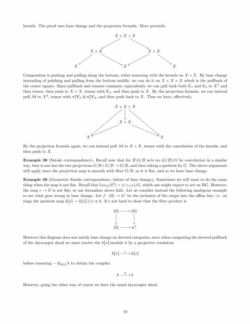
kernels. The proof uses base change and the projection formula. More precisely

X ˆX ˆX

''ww

X ˆX

''

X ˆX

ww ##X X X

Composition is pushing and pulling along the bottom, whist tensoring with the kernels on X ˆX. By base change

insteading of pulshing and pulling from the bottom middle, we can do it on X ˆX ˆX which is the pullback of

the center square. Since pullback and tensors commute, equivalently we can pull back both K1 and K2 to X3 and

then tensor, then push to X ˆX, tensor with K1, and then push to X. By the projection formula, we can instead

pull M to X3, tensor with π˚1K1 b π˚2K2, and then push back to X. Thus we have, effectively,

X ˆX ˆX

""

||

X ˆX

vv ((X X

By the projection formula again, we can instead pull M to X ˆX, tensor with the convolution of the kernels, and

then push to X.

Example 38 (Satake correspondence). Recall now that for BzGB acts on pGBqG by convolution in a similar

way, that is one has the two projections GBˆGB Ñ GB, and then taking a quotient by G. The above arguments

still apply since the projection map is smooth with fiber GB, so it is flat, and so we have base change.

Example 39 (Geometric Satake correspondence, failure of base change). Sometimes we will want to do the same

thing when the map is not flat. Recall that LocGpS2q “ peˆGeqG, which one might expect to act on BG. However,

the map e Ñ G is not flat, so our formalism above fails. Let us consider instead the following analogous example

to see what goes wrong in base change. Let f : t0u Ñ A1 be the inclusion of the origin into the affine line, i.e. on

rings the quotient map krxs Ñ krxspxq – k. It’s not hard to show that the fiber product is

t0u //

t0u

t0u // A1

However this diagram does not satisfy base change on derived categories, since when computing the derived pullback

of the skyscraper sheaf we must resolve the krxs-module k by a projective resolution

krxsx // krxs

before tensoring ´bkrxs k to obtain the complex

k0 // k

However, going the other way of course we have the usual skyscraper sheaf.

10

4.2 Resolving using dg algebras (in the affine case)

Remark 40 (Proof of base change in affine case). What went wrong here? Let’s recall that proof of base change

in the affine case. Take X “ SpecpRq, Y “ SpecpQq, Z “ Specpkq, then

X ˆZ Y //

X

Y // Z

base change says

M bLk Q “M bLR pRbk Qq

The problem is that one of these tensor products is not derived; if we were working with modules we could derive

the last fiber product and everything would follow from some homological algebra. If Q is flat over k then there is

no need to derive it. But otherwise, we need some way to resolve Q over k by free k-modules, but as an algebra.

The solution is semifree dg algebras.

Definition 41. Let M,N be two chain complexes, cohomologically graded (differentials increase degree). We define

their tensor product by the usual “convolution” tensor product of graded modules:

pM bNqk :“à

i`j“k

Mi bNj

and equip it with the differential (extended linearly):

dpmb nq :“ dpmq b n´ p´1qdegpmqmb dpnq

This defines a monoidal structure on chain complexes. A dg algebra over k is a category enriched over chain

complexes with a single object. More explicitly, it is a chain complex A equipped with a multiplicationm : AbAÑ A

which is a map of chain complexes. Even more explicitly, the multiplication should satisfy the rule:

dpx ¨ yq “ dpxq ¨ y ´ p´1qdegpxqx ¨ dpyq

A dg algebra is dg commutative if mpx, yq “ mpy, xq, i.e.

a ¨ b “ p´1qdegpaqb ¨ a

A morphism of dg algebras is a functor of such categories.

Example 42. Every k algebra is a dg algebra, concentrated in degree 0. It is dg commtuative if and only if it is

commutative.

Example 43. Let us define a free dg algebra on one generator in odd degree -1. That is, A “ krλs for degpλq “ ´1,

with zero differential. Note that by dg commutativity, λ ¨ λ “ ´λ ¨ λ, so in characteristic not 2, λ2 “ 0. Thus A is

a two dimension vector space, with one dimension in degree 0 and one dimension in degree -1.

Now let us define a free dg algebra on two generators in degree -1. That is, let A “ krλ1, λ2s with degpλiq “ ´1,

with zero differential. Then likewise one has λ2i “ 0, but one has that λ1 ^ λ2 “ ´λ2 ^ λ1. So A has dimension

four, with one dimension vector p1, 2, 1q. So we see that in odd degree the multiplication behaves like an exterior

product.

Example 44. Let us define a free dg algebra on one generator in degree -2. That is, let A “ krβs with degpβq “ ´2,

and zero differential. Then one has that A is infinite dimensional, with one dimension in every nonpositive even

dimension. Here the multiplication behaves like the usual multiplication in commmutative rings.

Definition 45. A dg algebra is semifree if the underlying graded algebra is free. A map of dg algebras is a

quasi-isomorphism if it induces an isomorphism in cohomology.

11

Example 46 (Koszul resolution). Let R “ krx1, . . . , xnspf1, . . . , frq. For each such R we have a resolution over

S “ krx1, . . . , xns called the Koszul resolution. Let V ˚ be an r-dimensional k-vector space spanned by dfi. Then

the Koszul resolution is given by

R » SrV s

where degpV q “ ´1 and the differential is given by dpdfiq “ fi. Note that the rest of the differentials are given by

the Leibniz rule, e.g.

dpdf ^ dgq “ f dg ´ g df

Example 47 (Self intersection of two origins). Going back to our original example, one comutes that

t0u ˆA1 t0u “ krλs

with degpλq “ ´1 and dpλq “ 0.

4.3 Some theory: what kind of category do dg algebras form?

Remark 48 (Derived rings). This subsection mostly serves to give an overview and references on the theory. What

we’ve done above essentially is, when considering an 8-stack as a functor Rng Ñ 8´Grpd, we’ve replaced the

category of rings with the category of dg algebras. There is a theoretically cleaner and more general category to

replace rings with, which we will, with vagueness, call derived rings. Lurie in his thesis Derived Algebraic Geometry

[Lu:Cr] discusses, along with dg algebras, two other candidates for derived rings: simplicial rings and E8 ring

spectra. In particular all three of these categories are (8, 1)-categories. It turns out that dg algebras are only

well-behaved in characteristic zero. Here, the monoidal Dold-Kan correspondence gives some kind of equivalence

between simplicial rings and dg algebras.

Remark 49 (Morphisms in the category of dg algebras). Dg algebras form an p8, 1q-category, though there is

some delicacy required in correctly defining the morphisms of dg algebras and considering them as a “space.” For

a treatment, see the survey article [To:DAG].

Remark 50 (Derived scheme). Toen [To:DAG] gives a notion of a derived scheme in characteristic zero using dg

schemes. An affine derived scheme is defined to be the “Spec” of a dg algebra. In general, a derived scheme is

a scheme X equipped with a sheaf of dg-algebras O‚X satisfying H0pX,O‚Xq “ OX and HipX,OXq quasicoherent

over OX . The functor from derived schemes into derived stacks is not fully faithful, see [BN:Loop] Remark 3.3.

Remark 51 (Derived stacks). In the way that stacks replaced Set with a suitable model category or infinity

category, one can do the same with Rng “ Affop. That is, a derived stack is a p8, 1q functor

dgAlgopÑ Spaces

satisfying a sheaf condition. Many details of the theory are being ignored in this exposition, for example what the

analogous etale or fppf topology is on these categories, and good notions of Artin stack, et cetera. Note that an

affine derived scheme (i.e. a dg-algebra) can be considered as a derived stack by an p8, 1q-version of the Yoneda

lemma.

4.4 Local systems revisited

Definition 52. We can now revise our definition of local systems, where X is a locally constant functor

LocGpXq “ MapDStpX,BGq

where the mapping space is now taken in the category of derived stacks.

Example 53 (Local systems on S2). From our above computations, one has

LocGpS2q “ pSpec Symkpg

˚r1sqqG

12

i.e. we use the Koszul resolution of the identity element of G, and tensoring with Oe kills all differentials. Note

that if we forget the derived structure, we obtain again LocGpS2qcl “ pt.

Remark 54. Note that S2 “ S1#S1 (the smash product, which is the categorical product in the category of based

spaces), and so we expect that (where Map denotes here based maps)

Map˚pS2, Xq “ Map˚pS

1#S1, Xq “ Map˚pS1,Map˚pS

1, Xqq “ ΩΩX,

the double based loop space.

Recall that ΩpBGq “ G. Then ΩpGq can be computed by

ΩG //

GˆGˆG G

π1“π2

ptePG

// G

One computes that Ω2pBGq “ Spec Symkpg˚r1sq, whose classical scheme is a point. This is obtained from LocGpS

2q

by affixing a base point, i.e. base changing away from BG:

Ω2BG » Spec Symkpg˚r1sq //

LocGpS2q » Spec Symkpg

˚r1sqG

ev˚

ptevx

// BG

Remark 55. This definition of local system differs from that in [AG:Sing], because we restrict our attention to the

case when X is a locally constant functor, where BunG and LocG are the same. These two diverge when one wants

to consider more generally, schemes, Artin stacks, and derived stacks.

References

[AG:Sing] Dima Arinkin, Dennis Gaitsgory, Singular support of coherent sheaves and the Geometric Langlands

conjecture, arXiv:1201.6343v4 2014.

[BN:Loop] David Ben-Zvi, David Nadler, Loop Spaces and Connections, arXiv:1002.3636v2, 2011.

[Lu:Cr] Jacob Lurie, Derived Algebraic Geometry, Ph.D. thesis, 2004.

[Pr:Stacks] Anatoly Pregel, Notes on stacks.

[To:DAG] Bertrand Toen, Derived Algebraic Geometry, arXiv:1401.1044v2, 2014.

13