CHILD LABOR, INCOME SHOCKS, AND ACCESS TO CREDIT*

Kathleen Beegle Development Research Group

World Bank

Rajeev H. Dehejia Department of Economics and SIPA

Columbia University and

NBER

Roberta Gatti Development Research Group

World Bank

Abstract

Although a growing theoretical literature points to credit constraints as an important source of inefficiently high child labor, little work has been done to assess its empirical relevance. Using panel data from Tanzania, we find that households respond to transitory income shocks by increasing child labor, but that the extent to which child labor is used as a buffer is lower when households have access to credit. These findings contribute to the empirical literature on the permanent income hypothesis by showing that credit-constrained households actively use child labor to smooth their income. Moreover, they highlight a potentially important determinant of child labor and, as a result, a mechanism that can be used to tackle it.

World Bank Policy Research Working Paper 3075, June 2003 The Policy Research Working Paper Series disseminates the findings of work in progress to encourage the exchange of ideas about development issues. An objective of the series is to get the findings out quickly, even if the presentations are less than fully polished. The papers carry the names of the authors and should be cited accordingly. The findings, interpretations, and conclusions expressed in this paper are entirely those of the authors. They do not necessarily represent the view of the World Bank, its Executive Directors, or the countries they represent. Policy Research Working Papers are available online at http://econ.worldbank.org.

* We thank Jishnu Das, John Strauss, Steven Zeldes, and seminar participants at George Washington University, the NEUDC 2002 conference, the World Bank, and the World Bank Economists’ Forum for useful comments. Dehejia acknowledges the National Bureau of Economic Research and the Industrial Relation Sections, Princeton University, for their kind hospitality. Support from the World Bank’s Research Committee is gratefully acknowledged. Please address correspondence to rgatti@worldbank.org.

Pub

lic D

iscl

osur

e A

utho

rized

Pub

lic D

iscl

osur

e A

utho

rized

Pub

lic D

iscl

osur

e A

utho

rized

Pub

lic D

iscl

osur

e A

utho

rized

1

1. Introduction

This paper examines the relationship between household income shocks, access to credit, and child

labor. In particular, we investigate the extent to which income shocks lead to increases in child

labor, and whether households with access to credit can mitigate the effects of these shocks.

These questions are important for three reasons. First, they point to a potentially important

determinant of child labor and, as a result, at mechanisms that can be used to tackle it. This is

particularly relevant since child labor is often viewed primarily as a consequence of poverty. For

example, in a recent publication, the World Bank defined child labor as “one of the most

devastating consequences of persistent poverty” (Fallon and Tzannatos [1998]). To some extent,

the stylized facts bear out this view. In 1995, the incidence of child labor was 2.3 percent among

countries in the upper quartile of GDP per capita, and 34 percent among countries in the lowest

quartile of GDP per capita (see Dehejia and Gatti [2002] and Krueger [1996]). If poverty is the

main cause of child labor, then the prevalence of child labor should decrease as countries develop.

However, the relationship between poverty and child labor has been put into question by some

recent within-country studies.1 In particular, imperfections in labor markets, education and – the

focus of this paper – credit markets might be at the root of child labor. In this case, policies

designed to correct such imperfections directly might be an efficient means of tackling child labor.

Second, in the theoretical literature on child labor (reviewed below), lack of access to credit

plays a central role in determining the prevalence of child labor. From the household’s point of

view, child labor entails a trade-off between immediate benefits (increased current income) and, to

the extent it interferes with the accumulation of the child’s human capital, potential long-run costs

1 In their review of several studies, Canagarajah and Nielsen [1999] do not find clear evidence that poverty is associated with higher incidence of child labor within countries. In their study of Ghana, Boozer and Suri [2001] do not find a link between poverty and child labor, concluding that policies to alleviate poverty may not be appropriate to reduce child labor. Using data from Ghana and Pakistan, Bhalotra and Heady [2001] provide evidence that children of land-rich households are more likely to work (and less likely to be in school) than their counterparts in land-poor households. They label this finding the “wealth paradox” since it challenges the notion that child labor is observed

2

(lower future earnings potential). A number of recent models show that, by preventing households

from trading off resources intertemporally in an optimal way, credit constraints give rise to

inefficiently high child labor.2

Two key economic variables that influence households’ demand for and ability to smooth

resources inter-temporally are income shocks and access to credit. Despite their theoretical

centrality (for example, see the discussion in Grootaert and Patrinos [1999]), little empirical

research has been undertaken to examine the connection between income shocks, access to credit,

and child labor. Indeed, to our knowledge, this is among the first studies explicitly examining this

link.

Third, our work relates to an important literature on the permanent income hypothesis,

income smoothing, and credit constraints. In particular, our work provides a bridge between

studies such as Zeldes [1989], who documents the importance of credit constraints in preventing

optimal smoothing of consumption over time, and Townsend [1994], who demonstrates that

household consumption follows a smoother path than household income. As documented

extensively in work by Morduch [1994, 1995, 1999], if households succeed in smoothing their

consumption profile, but are credit constrained, they are likely to resort to mechanisms other than

borrowing to cope with income shocks. This paper examines one such mechanism, namely child

labor. In this context, our work is complementary to Jacoby and Skoufias [1997] and Kochar

[1999], who examine respectively the role of schooling and parental labor supply as buffers to

income shocks.

more often among children in poor households. A combination of labor market failures and ill-functioning land markets can explain this result. 2 In outlining child labor issues and directions for the World Bank, Fallon and Tzannatos [1998] point out that child labor can have additional costs in terms of harmful effects on physical health and mental well-being (such as psychological and social adjustment) of children. Moreover, others contend that the working conditions for children are far below those of adults in terms of hours worked, wages, and safety. 3 Fallon and Tzannatos [1998] point out that child labor can have additional costs in terms of harmful effects on physical health and mental well-being (such as psychological and social adjustment) of children. Moreover, others contend that the working conditions for children are far below those of adults in terms of hours worked, wages, and safety.

3

Using four rounds of household panel data from the Kagera region of Tanzania, we show

that transitory income shocks – as proxied by crop accidentally lost to insects, rodents, and fire –

lead to significantly increased child labor. Moreover, we find that households with collateralizable

assets – which, in line with the existing literature (see for example Jacoby [1994]) we interpret as a

measure of access to credit – are better able to offset the effects of these shocks. It is of course

possible that a higher level of collateralizable assets mitigates the effect of child labor for reasons

other than the ability to borrow. One of these confounding effects is a wealth effect and another

possibility is that the level of collateralizable assets is correlated with unobservables such as a

household’s social network. Nonetheless, we find that our results remain robust after controlling

for other sources of wealth and for household fixed effects.

The paper is organized as follows. In Section 2, we provide a brief review of the literature.

The empirical strategy is outlined in Section 3. In Section 4, we describe our data. In Section 5 we

present our results and Section 6 concludes.

2. Literature Review

2.1 Theoretical Perspectives on Child Labor

Basu [1999] partitions the child labor literature into two groups: papers which examine intra-

household bargaining (between parents, or parents and children) and those which examine extra-

household bargaining (where the household is a single unit and bargains with employers).

In the intra-household bargaining framework, child labor is the outcome of an optimization

process which places different weights on household members, for example parents and children

(see Bourguignon and Chiappori [1994] and Moehling [1995]), or the mother (who altruistically

cares for the children) and the father (who cares for himself in addition to the family; see Galasso

[1999]). The weight that each member receives can depend upon his or her contribution to the

family’s resources. Collectively, child labor may be beneficial because it contributes to family

4

income, and it may be desirable to the child because it increases his or her weight in the family’s

decision function. Within this framework, key variables in determining child labor are those that

influence the relative bargaining strength of different members of the household. This could

include wealth, the number, age, and gender of children, and individual wages as well as the set of

opportunities for education available to children such as access to and quality of schooling.

The inter-household bargaining framework considers each household as a unitary entity

(see Becker [1964] and Gupta [2000]). The motivation behind this approach is that children’s

bargaining power is inherently very limited. The parents and the employer bargain about the

child’s wage and the fraction of that wage to be paid as food to the child. Within this framework,

the key variables are those that determine the relative bargaining strength of the household vis à vis

the employer. These include, amongst others, household wealth and variables such as the access to

credit.4

The unitary model of the family à la Becker [1964] is best suited to understanding the role

of borrowing constraints as determinants of child labor. Analytically, the question is closely

related to the bequests literature, which has highlighted that the non-negativity constraints in

bequests can lead to an inefficient allocation of resources within the family (see for example

Becker and Murphy [1988]). A recent strand of theoretical literature has addressed the implications

of this for child labor (Parsons and Goldin [1989], Baland and Robinson [2000], and Ranjan

[2001]). In particular, these papers show that if parents care about their children, but parents’

bequests are at a corner, child labor is generally not efficient. The basic intuition is that child labor

creates a trade-off between current and future income (Baland and Robinson [2000]). Putting

children to work raises current income, but by interfering with children’s human capital

development, it reduces future income. The future income is, of course, realized by the children

4 Most theoretical models of child labor (and certainly the empirical literature) focus on supply-side factors. Canagarajah and Nielsen [1999] outline demand-side factors which can play critical roles in perpetuating child labor.

5

and not the parents. Thus, if bequests are positive, parents can compensate themselves for foregone

current income by reducing bequests. Instead, when parents do not leave bequests for their

children (for example, if they are poor) or financial market imperfections do not allow parents to

trade off old-age income with current resources, parents will have their children supply “too much”

labor.

This theoretical approach suggests that the availability of credit should be a factor that

predicts the incidence of child labor. Moreover, we can interpret evidence of such an effect as an

indication that observed child labor is inefficiently high.

2.2 Empirical Work on Child Labor

Although the recent theoretical literature highlights income shocks and borrowing constraints as an

important source of inefficiency in the allocation of resources within the family and, in particular,

of inefficiently high child labor (Ranjan [2001] and Baland and Robinson [2000]), the link between

income shocks, access to credit, and child labor remains largely unexplored in the empirical

literature.

There are a wide range of empirical studies of child labor at the micro-level using

household survey datasets. These studies tend to estimate reduced-form participation equations for

child work. For example, in a recent volume, Grootaert and Patrinos [1999] review findings of

studies of child labor from Côte D’Ivoire, Colombia, Bolivia, and the Philippines. Canagarajah and

Nielsen [1999] review findings from five studies from Côte D’Ivoire, Ghana, and Zambia. These

are only several of a much wider list of studies in this area which have contributed to a better

understanding of the factors that influence child labor. A consistent finding of these studies is that

the child’s age and gender, education and employment of the parents, and rural versus urban

These include the non-pecuniary characteristics of children that may make them desirable employees for employers, such as being more willing to take orders and do monotonous work, and less aware of rights, among other factors.

6

residency are robust predictors of child labor. Few studies examine child labor in Tanzania using

household survey data (see Beegle [1998]), although several studies focus on schooling

determinants in Tanzania.5

There are a number of studies that assess the relationship between schooling outcomes and

shocks. Of course, it is not obvious that for children there is a one-to-one trade-off between time

spent in school and time spent working. Many children not enrolled in school are not necessarily

working and, in many cases, enrolled children combine their schooling with work. Furthermore,

hours in either activity may be sufficiently low on average that an increase in time spent in one

activity will not crowd out time spent in another, as opposed to crowding out leisure time (for

example, see the evidence in Ravallion and Wodon [2000]).

Jacoby [1994] examines the relationship between borrowing constraints and progression

through school among Peruvian children. He concludes that lack of access to credit perpetuates

poverty because children in households with borrowing constraints begin withdrawing from school

earlier than those with access to credit. Jacoby and Skoufias [1997] is the first empirical work that

rigorously addresses the issue that poor households lacking access to credit markets might draw

upon child labor when faced with negative income shocks. Using data on school attendance

patterns from six Indian villages, the authors conclude that fluctuations in school attendance are

used by households as a form of self-insurance. However, these studies focus only on schooling

and not on child labor activities, which would likely be more directly affected by income shocks

and inability to access credit.

Dehejia and Gatti [2002] use cross-country data on child labor to investigate the association

between child labor and access to credit (as proxied by financial development) across countries.

5 These studies examine a range of schooling outcomes, such as: the general decision to enroll at primary or secondary levels (Al-Samarrai and Peasgood [1998] and Mason and Khandker [1997]); delayed enrollment decisions (Bommier and Lambert [2000]); urban-rural differentials (Al-Samarrai and Reilly [2000]); the impact of own health and illness among household member on attendance (Burke [1998] and Burke and Beegle [2003]); and the relationship between orphanhood status and enrollment (Ainsworth et al [2002]).

7

They find a significant negative and robust relationship between the two variables, which is

particularly sizeable in poor countries. Moreover, their evidence suggests that in the absence of

developed financial markets, households resort substantially to child labor in order to cope with

aggregate income variability.

The only work that we are aware of that uses micro data to examine the link between credit

constraints and child labor is Edmonds [2002] and Guarcello et al. [2002]. Edmonds [2002]

examines the impact of the South African old-age pension on the child labor of households that are

headed by senior citizens. He, like us, finds evidence of credit constraints, but using a different

strategy. We discuss his work again in the next section. Guarcello et al. [2002] analyze the

response of child labor to broadly defined income shocks (loss of employment, death in the family,

droughts in the region, etc.) in Guatemala. They identify a sub-sample of credit-constrained

households using information on denial of credit for households that applied and self-reported

information on why a family was not able to apply for credit among non-applicants. They find that

credit rationing is associated with higher child labor and that shocks significantly increase the

proportion of working children. The results in Guarcello et al. [2002] are complementary to ours

although they do not evaluate the differential impact of shocks in households facing different levels

of credit constraints. While the authors have the advantage of availing themselves of direct

information on access to credit, in their setup lack of access to credit might reflect household

characteristics associated with attitudes towards child labor rather than financial market

imperfections. Similarly, the cross-sectional structure of their data does not allow them to fully

disentangle the extent to which shocks are exogenous.

8

2.3 The Permanent Income Hypothesis Literature

As indicated in the introduction, this paper bridges two strands of the empirical literature on the

permanent income hypothesis (PIH).

One strand of this literature examines whether credit constraints can be used to account for

apparent rejections of the PIH. In particular, Zeldes [1989] splits households in his sample by their

holding of financial assets and examines the extent to which the Euler equation implied by the PIH

hold for both groups. He concludes that credit constraints are an important impediment to

intertemporal consumption smoothing for many households. A second strand of the literature

examines the extent to which households can insure themselves against idiosyncratic income

shocks. Studies showing that the profile of household consumption is smoother than the profile of

household income indicate that households are able to some extent to smooth away income shocks

(see Deaton [1992], Morduch [1995], and Townsend [1994]). The two results together suggest that

households – even when credit constrained – are resorting to some means other than borrowing (or

explicit insurance) to smooth away shocks.

In this paper we examine whether child labor is one such mechanism that can account for

household income smoothing. In particular, we examine the response of agricultural households to

a transitory income shock. To the extent that the shock is transitory, the PIH suggests that

households should borrow to smooth away much of the shock. In this context, our test has two

parts. First, do households with limited borrowing capacity indeed increase child labor in response

to a transitory shock? And, second, is this effect mitigated for households with greater borrowing

capacity? As such, our work is in line with Paxson [1992], who documents that households save

most of their transitory income and Jacoby and Skoufias [1997], who demonstrate households

adjust their children’s school attendance in response to shocks.

Edmonds [2002] uses a different, albeit related, identification strategy. He examines the

impact of a permanent increase in old-age pension support in South Africa. Whereas our

9

identification of credit constraints is based on finding an effect of a transitory income shock,

Edmonds examines a fully anticipated increase in income. If households are not credit constrained,

then they can borrow against the future receipt of their old-age pension, and there should be no

adjustment in child labor at the time the household actually begins to receive its pension. The two

approaches are clearly complementary. A caveat to Edmonds’ approach is that households may not

borrow against their future old-age pension simply because they are myopic, not credit constrained.

In this case, the effect he estimates would simply be a wealth effect. An advantage of our approach

is that households do not have to be forward-looking to respond to a negative income shock. Of

course, our key underlying assumption is that the income shock that we examine is indeed

transitory.

3. Empirical Strategy and Specification

In this section, we outline the empirical strategy and specification we employ to identify the effects

of income shocks and access to credit on child labor choices within households. We are interested

both in the direct effect of an income shock as well as in the extent to which access to credit helps

families to smooth away the impact of a shock.

The literature on consumption and savings distinguishes between two types of shocks –

transitory and permanent. The theoretical effect of these shocks on time allocation and borrowing

decisions are different. If we believe that income affects child labor outcomes negatively (with a

stronger relationship among the poor), we would expect a permanent negative income shock to

increase child labor, especially for children in poor households. Furthermore, we do not expect

households to borrow to offset the effect of such shocks. Conversely, credit or self-insurance

through accumulated savings can be an effective tool in smoothing transitory shocks. Instead,

increasing child labor in response to a transitory shock carries important costs for human capital

development because of the often-irreversible disruption in schooling.

10

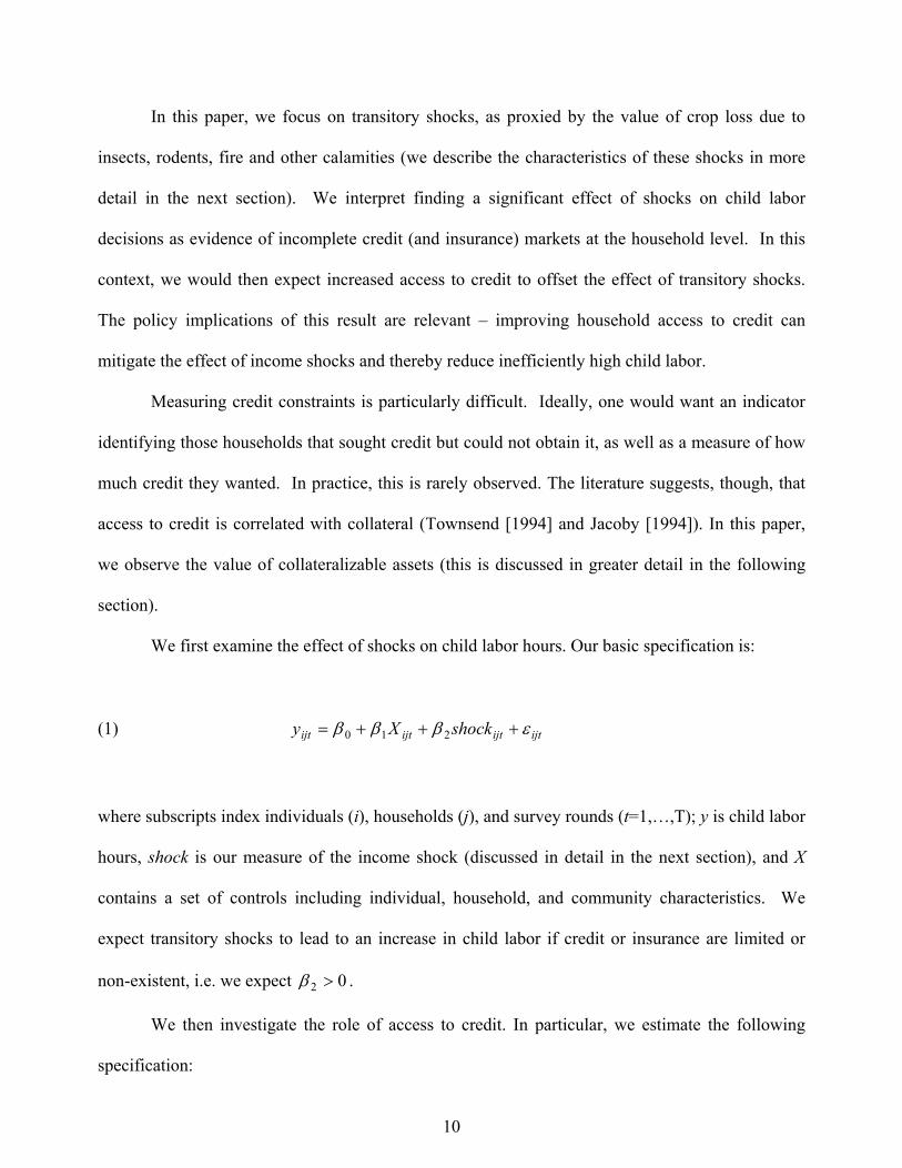
In this paper, we focus on transitory shocks, as proxied by the value of crop loss due to

insects, rodents, fire and other calamities (we describe the characteristics of these shocks in more

detail in the next section). We interpret finding a significant effect of shocks on child labor

decisions as evidence of incomplete credit (and insurance) markets at the household level. In this

context, we would then expect increased access to credit to offset the effect of transitory shocks.

The policy implications of this result are relevant – improving household access to credit can

mitigate the effect of income shocks and thereby reduce inefficiently high child labor.

Measuring credit constraints is particularly difficult. Ideally, one would want an indicator

identifying those households that sought credit but could not obtain it, as well as a measure of how

much credit they wanted. In practice, this is rarely observed. The literature suggests, though, that

access to credit is correlated with collateral (Townsend [1994] and Jacoby [1994]). In this paper,

we observe the value of collateralizable assets (this is discussed in greater detail in the following

section).

We first examine the effect of shocks on child labor hours. Our basic specification is:

(1) ijtijtijtijt shockXy εβββ +++= 210

where subscripts index individuals (i), households (j), and survey rounds (t=1,…,T); y is child labor

hours, shock is our measure of the income shock (discussed in detail in the next section), and X

contains a set of controls including individual, household, and community characteristics. We

expect transitory shocks to lead to an increase in child labor if credit or insurance are limited or

non-existent, i.e. we expect 02 >β .

We then investigate the role of access to credit. In particular, we estimate the following

specification:

11

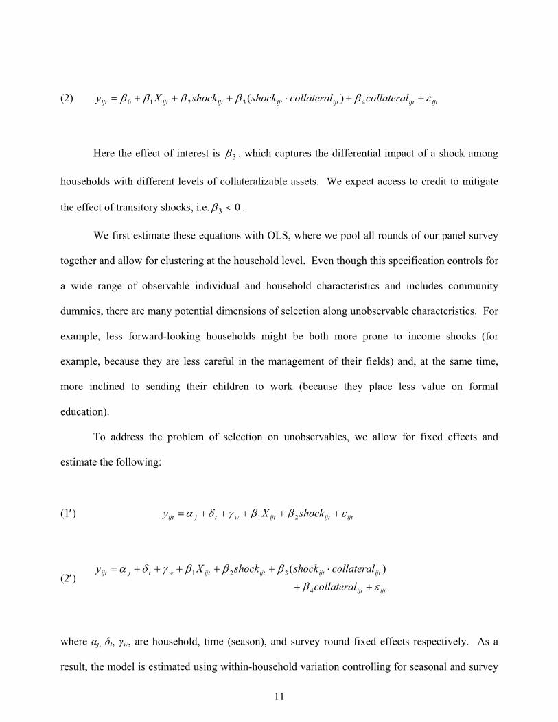
(2) ijtijtijtijtijtijtijt collateralcollateralshockshockXy εβββββ ++⋅+++= 43210 )(

Here the effect of interest is 3β , which captures the differential impact of a shock among

households with different levels of collateralizable assets. We expect access to credit to mitigate

the effect of transitory shocks, i.e. 03 <β .

We first estimate these equations with OLS, where we pool all rounds of our panel survey

together and allow for clustering at the household level. Even though this specification controls for

a wide range of observable individual and household characteristics and includes community

dummies, there are many potential dimensions of selection along unobservable characteristics. For

example, less forward-looking households might be both more prone to income shocks (for

example, because they are less careful in the management of their fields) and, at the same time,

more inclined to sending their children to work (because they place less value on formal

education).

To address the problem of selection on unobservables, we allow for fixed effects and

estimate the following:

(1′) ijtijtijtwtjijt shockXy εββγδα +++++= 21

(2′) ijtijt

ijtijtijtijtwtjijt

collateral

collateralshockshockXy

εβ

βββγδα

++

⋅+++++=

4

321 )(

where αj, δt, γw, are household, time (season), and survey round fixed effects respectively. As a

result, the model is estimated using within-household variation controlling for seasonal and survey

12

round effects. Note that fixed effects at the household level subsume community-level

unobservable characteristics. However, we cannot rule out time-varying household-level

unobservable characteristics.

4. Data Description and Summary Statistics

The data for this study are from a panel dataset for the Kagera region in Tanzania. The Kagera

Health and Development Survey (KHDS) was part of a research project conducted by the World

Bank and the University of Dar es Salaam. The KHDS surveyed over 800 households in the region

up to four times from 1991-1994 with an average interval between surveys of six to seven months.6

Households are drawn from 51 communities, mostly villages, in the six districts of Kagera.

This dataset has several features that make it particularly appropriate for the proposed

analysis. First, the detailed household survey has a wide array of individual and household

characteristics, including information on time use of all household members aged seven and older.

This includes time spent in the previous week working on household businesses (farm and non-

farm), for wages in non-household business, and in household chores. The household survey also

includes information on crop loss, as well as measures of physical and financial assets in each of

the four interviews. The data are longitudinal and, as such, they allow us to test and control for

unobservable variables that may bias cross-sectional results.

Our definition of child labor is the total hours in the last week spent working in economic

activities and chores (including fetching water and firewood, preparing meals, and cleaning the

house). Economic activities for children consist predominately of farming, including tending crops

in the field, processing crops, and tending livestock. Few children are engaged in wage

employment or non-farm family businesses. This is consistent with reports of limited child-labor

6 The explicit objectives of the KHDS were to measure the economic impact of fatal illness (primarily due to HIV/AIDS) in the region and to propose cost-effective strategies to help survivors. For more information about this project, see Ainsworth et al. [1992] and World Bank [1993].

13

markets from the community data. We include chores as well as economic activities for two

reasons. First, the concept of child labor (by ILO standards) is not restricted to only economic

activities.7 Second, in the largely rural sample of households in this study, it may be difficult to

distinguish time in household chore activities and time spent preparing subsistence food crops. For

our study, we focus on two age samples. Our primary age group includes children 10-15 years old.

We also include a second group, children 7-15 years old. Given the well-documented low

enrollment levels and delayed enrollment in Tanzania, along with the low hours of work among

younger children (7-9), our main focus are children of age 10 and older. The upper age range for

child-labor studies is typically 14 or 15 years, the age of completed primary schooling if enrolled

on time.

Table 1 presents summary statistics of the sample in our study, broken down by the three

samples on which the regressions are run. In addition, the last 2 columns show summary statistics

for the main sample separated into those children in households that had experienced an income

shock and those that had not. In the pooled data, children worked on average about 21 hours in the

previous week. Mean hours as well as most other covariates are similarly distributed in households

with and without a shock. More than 90 percent of children worked at least 1 hour in the last week.

About one-third of children reside in households that report some crop loss.8 About one-half of

children reside in households with any durables, our primary indicator of collateral. Among those

households that experienced a shock, the total value of the shock is about twice (in log terms) the

value of per capita durable goods. The prevalence of alternative wealth indicators, cash holdings

and physical assets, is larger. Nearly three-quarters of children live in households with some cash

and all children live in households with some physical assets (including the value of land, business

7It should also be mentioned that the concept of child labor does not necessarily refer to simply any work done by a child, but, rather, work that stunts or limits the child’s development or puts the child at risk. However, in survey data it is difficult (perhaps impossible) to appropriately isolate the portion of time spent working on the farm that qualifies under this very nuanced definition. Therefore, we follow the standard convention in the empirical literature. 8 For zero values of shock, durables, cash, and physical assets, the bottom value is coded at 1.

14

equipment, livestock, and dwellings). The average household size is quite large, over 7 members

on average. In part, this reflects the sample of households with children; in the entire sample

(including households with no children age 10-15), the average size is about 5.7 members. Levels

of parental education are extremely low. Few children have fathers who had attended school

beyond the primary level (12 percent of children) and almost none had mothers with more than

primary schooling (2 percent).

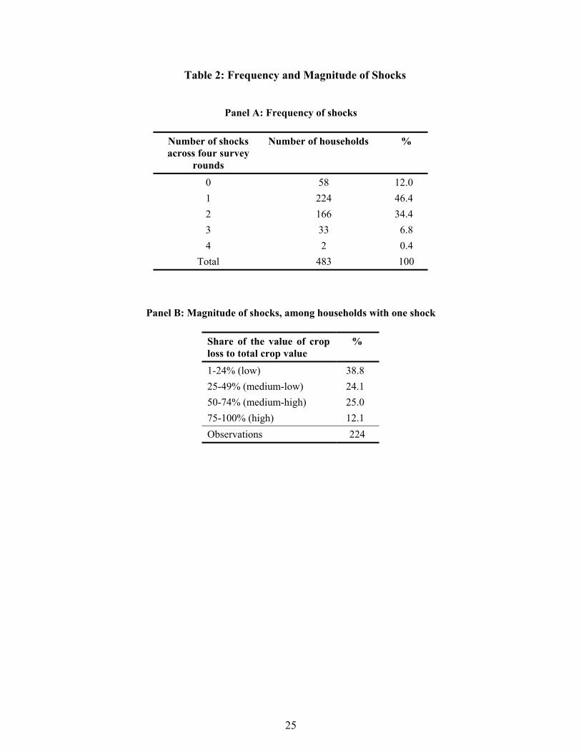
Turning to our measure of income shock, for the identification strategy to be credible, we

ideally want an income shock that is: of a sufficient magnitude to potentially affect household time

allocation; exogenous to child labor decisions; and transitory. The data include reports of the value

of crop loss due to insects, rodents, and other calamities (such as fire) in each survey round. We

compute the total value of crop loss for all crops farmed. This measure of income shock has

several advantages. First, since agriculture is the main economic activity in the Kagera region,

many households experience a shock and these shocks are extremely relevant with respect to

household income. As reported in Table 2, Panels A and B, 88 percent of households experience a

shock during one of the four survey rounds, and around 50 percent of those households

experiencing one shock lose 25 to 75 percent of the value of their crops to calamities. Hence these

shocks are common, and can be significant in magnitude.

Second, these shocks are plausibly exogenous and transitory. Table 3, Panel A, shows the

correlation between the occurrence of a shock and several household characteristics. As discussed

in Morduch [1994], in general there may be reasons to believe that poorer households (with a high

prevalence of child labor) may also be more prone to income shocks. However, none of the

standard household covariates predicts shocks in our data. Moreover, controlling for household

characteristics, shocks do not appear to be correlated over time.

One might argue that households can use information not available through the survey to

forecast shocks. If that is the case and families actively use child labor as a buffer against shocks,

15

they might adjust child labor supply in advance. However, we find that child labor in period t-1

does not significantly predict shocks (for value as well as share of crop loss) in period t (Table 3,

Panel B). Overall, this evidence suggests that the value of crop loss provides us with credible

transitory, exogenous, and unanticipated shocks.

We measure access to credit with collateralizable assets. This is in keeping with the related

literature, including Zeldes [1989] and Jacoby [1994]. Consistent with this approach, fully 80

percent of all lenders (banks, NGOs, private individuals) reported requiring collateral for loans.9

As noted by Jacoby, it is important to select a class of assets that is associated with a household’s

borrowing capacity, but is not directly linked to its demand for child labor. Collateralizable assets

in this setting include the value of durable goods, such as radios, bicycles, fans, lamps and pots.

This excludes cash holdings, business, and land value which might be directly correlated with

demand for child labor within the household. In the regressions, we measure collateral as the (log)

value of durable assets per household member.

5. Results

We first discuss the effect of income shocks on child labor as estimated with OLS and fixed effects.

We then present estimates for the interacted model with shocks and collateral. Finally, we conduct

several robustness checks, including using alternative definitions for shocks and access to credit,

and running the specification on a suitably restricted sample.

5.1 The Effect of Shocks

Table 4, column 1, reports OLS estimates of the effect of the income shock on child labor for

children between the age of 10 and 15. An income shock is associated with significantly higher

child labor. A one standard deviation income shock is associated with a 10 percent increase in

16

mean hours in the last week. This effect is robust in magnitude and significance to including

community dummies in the regression (column 2).

Column 3 reports the estimates from a household fixed effect model. Since we are now

controlling for a substantial range of variables (including effects related to households, seasons,

and survey rounds), the estimated coefficient is smaller than the OLS estimate (0.22 vs. 0.33) but

still statistically significant at the 1 percent level. This result confirms that the correlation between

shocks and child labor is not driven by spurious unobserved family effects. We obtain similar

results if we expand our sample to the 7-15 age range (column 4). Not surprisingly, we find that

the magnitude of the coefficient on shocks decreases once the sample is enlarged to include 7-10

year old children. First, younger children work less on average. Moreover, we expect their work

supply to be less responsive to shocks – to the extent that parents perceive them as less productive

than their older siblings, they will be more willing to send the older children to work in response to

a shock. We interpret all of these findings as evidence that households resort to child labor

substantially when coping with income shocks.

5.2 The Effect of Credit

In Table 5, we estimate equations (2) and (2′) using OLS (column 1) and fixed effects (column 2

for 10-15 year olds, column 3 for 7-15 year olds). These models allow for both income shocks and

access to credit, and in particular, for a differential response of child labor hours to shocks in

households with different levels of collateralizable assets. Columns 4-7 extend the model to

include additional wealth controls and restrict the sample to households with land.

First, note that the effect of the income shock is stable across columns 1-3 and similar in

magnitude and significance to the estimates reported in Table 4.

9 The community questionnaires provided this information.

17

The OLS estimates (column 1) return a negative and significant coefficient on collateral,

but no significant effect for the interaction between collateral and shock. As discussed in Section

3, OLS estimates are potentially biased due to selection effects. There are two sources of concern.

First, households with higher levels of collateral may also tend to have lower levels of child labor,

simply due to wealth effects. Second, unobservable factors such as motivation and inter-temporal

discount factors might lead some households to value the long-term benefits of education as well as

to undertake actions to avoid income shocks. In both cases the between-household association of

access to credit and child labor would be non-causal. Fixed effects in column 2 allow us to focus

on the within-household relationship between collateral and income shocks. There we see that the

estimated impact of collateral is completely absorbed by fixed effects – in particular, it switches

sign and becomes insignificant. Conversely, the interaction between shock and collateral is

consistently negative and significant in the fixed effect estimates. This suggests that the

availability of credit mitigates the effect of shocks. In particular, a one standard deviation increase

in the income shock is associated with a 10 percent increase in child labor hours for households

without durable assets, whereas in a household with a median level of durables, the increase in

child labor hours is 5 percent. In other words, the availability of a typical level of collateral offsets

half the effect of a shock.

Estimates are similar in significance and magnitude for the sample of children between age

7 and 15 (column 3) and are in line with results in Table 4, column 2.

It could be argued that the value of durables simply captures a wealth effect as opposed to

the effect of access to credit. In order to preclude this alternative explanation, in columns 4-6 we

control for other measures of wealth, namely cash holdings and per capita physical assets (land,

equipment, and tools). Under these alternative specifications, the interaction of interest remains

significant and stable, while the direct effect of the additional wealth controls is not significant.

18

To confirm the validity of our estimated effects, we examine the subset of households that

is most directly affected by agricultural shocks. We do so in two ways. First, we include an

indicator for whether the head of the household’s main activity is farming. This indicator is not

significant and its inclusion does not affect our estimates of interest (column 5). However, this

indicator is not always a precise measure of the extent to which farming contributes to family

income. As an alternative, we use the size of land ownership as an indicator of whether farming is

likely to be the main income source for the whole household. We confine ourselves to the sample

of households with more than one acre of land (anecdotally, this is generally considered the

minimum land size for subsistence) – and also exclude the top 1 percent of landowners. The results

are virtually unchanged.

It is also possible that these additional sources of wealth matter differentially when the

household is faced with an income shock. In particular, we would expect that households tap their

cash holdings first when faced with a shock but resort to mortgaging land – for which there exist

only thin markets in the region – only as an extreme remedy to a transitory shock. As such, cash

can in principle perform a similar function to collateralizable durables, while ownership of physical

assets should not, on average, matter in the interaction with the shock. It is also possible that

wealth variables proxy for the extent of households’ social networks, which arguably are more

valuable in times of need. When we include these three sources of wealth and their interaction with

the shock in the same specification and estimate it with fixed effects (column 7), income shocks

remain strongly and positively associated with child labor. However, these additional wealth

variables are highly collinear, and as a result the statistical significance of our coefficient of interest

diminishes, although its magnitude is robust.

19

5.3 Robustness Checks

In Table 6, we examine the sensitivity of our results to the definition of income shock and

collateral. One concern with our definition of income shock is that we might be more likely to

observe large crop losses among richer households – the more you have, the more you would

expect to lose if you have a loss. However, an indicator of whether a significant crop loss occurred

would still identify households without necessarily inducing a strong correlation with the level of

income. When we use this alternative definition of shock (adjusted to encompass income shocks of

some relevance, above 10 percent of the total value of crop), we find that, similar to Table 5,

shocks are positively and significantly associated with child labor hours (Table 6, column 1). Crop

losses of 10 percent or more of overall crop value are associated with a 7 percent increase in child

labor hours. Moreover, in column 2 we find that the interaction between this new measure of

shock and collateral is negative and significant. Children in households with no durables have 12

percent higher labor hours (evaluated at mean hours) when crop losses occur, compared to 4

percent higher hours for children in households with median per capita durable assets. Column 3

reports the results for the sample restricted by land ownership. The increase in child labor hours

associated with income shocks widens between children in households with and without

collateralizable assets (8 percent and 19 percent, respectively).

We then examine alternative definitions of collateral while returning to our initial measure

of income shock. Because of the large share of zeros in the distribution of durables (somewhat less

than 50 percent), it is reasonable to examine the robustness of our result to a specification that uses

an indicator for zero versus positive levels of collateral. In column (4), we note that the estimated

coefficient on the interaction of interest is unchanged in sign and significance, although of course

the magnitude changes since collateral is now a dummy rather than a continuous variable. One

could also argue that it is the total value of durables in the household, as opposed to its per capita

value, that matters as collateral. To account for this possibility, we use the total durable value as an

20

alternative measure of collateral in column 5. When we do so, the estimates of our effects of

interest are virtually unchanged, even while controlling for cash holding and value of physical

assets (column 5).

6. Conclusions

This paper has examined the link between transitory income shocks, access to credit, and child

labor. We show that child labor increases significantly in response to crop losses due to calamities

such as fire, insects, rodents, etc. Moreover, we show that the availability of collateralizable assets

offsets the effect of income shocks on child labor, even when controlling for other sources of

wealth in the family and for household level unobservables. This result is important because it

corroborates a large theoretical literature on the relevance of credit constraints in predicting child

labor, points to child labor as one of the mechanisms that households use to smooth transitory

income shocks, and finally suggests that expanding access to credit might be effective in mitigating

the prevalence of child labor.

21

REFERENCES

Ainsworth, M., G. Koda, G. Lwihula, P. Mujinja, M. Over and I. Semali, “Measuring the Impact of fatal Adult Illness in Sub-Saharan Africa.” Living Standards Measurement Study no. 90. World Bank, Washington, D.C. (1992). Ainsworth, M., K. Beegle, and G. Koda, “The Impact of Adult Mortality of Primary School Enrollment in Northwestern Tanzania.” Africa Region Human Development Working Paper Series, World Bank (2002). Al-Samarrai, S. and B. Reilly, “Urban and Rural Differences in Primary School Attendance: An Empirical Study for Tanzania.” Journal of African Economies, IX (2000), 430-474. Al-Samarrai, S. and T. Peasgood, “Education attainments and household characteristics in Tanzania.” Economics of Education Review, XVII (1998), 395-417. Baland, J. and J. Robinson, “Is Child Labor Inefficient?” Journal of Political Economy, CVIII (2000), 663-679. Basu, K., “Child Labor: Cause, Consequence, and Cure with Remarks on International Labor Standards,” Journal of Economic Literature, XXXVII (1999), 1083-1119. Becker, G., Human Capital, New York: Columbia University Press, 1964. Becker, G. and K. Murphy, “The Family and the State,” Journal of Law and Economics, XXXI, (1988), 1-18. Beegle, K., “The Impact of Adult Mortality in Agricultural Households: Evidence from Rural Tanzania,” mimeo. (1998). Bhalotra, S. and C. Heady, “Child Farm Labour: The Wealth Paradox,” mimeo. (2001). Blunch, N. and D. Verner, “Revisiting the Link between Poverty and Child Labor,” World Bank Policy Research Working Paper no. 2488. (2000) Bommier, A. and S. Lambert, “Education Demand and Age at School Enrollment in Tanzania,” Journal of Human Resources, XXXV (2000), 177-203. Boozer, M. and T. Suri (2001) “Child Labor and Schooling Decisions in Ghana,” mimeo. Bourguignon, F. and P.A. Chiappori, “The Collective Approach to Household Behavior,” in The Measurement of Household Welfare, Richard Blundell, Ian Preston, and Ian Walker, eds. Cambridge: Cambridge University Press, 1994. Burke, K. and K. Beegle, “Why children aren’t attending school: The case of rural Tanzania,” mimeo. (2003). Burke, K, “Investing in children’s human capital in Tanzania: Does household illness play a role?” Dissertation, SUNY Stony Brook, Stony Brook , NY. (1998).

22

Canagarajah, S. and H. Nielsen, “Child Labor and Schooling in Africa: A Comparative Study,” mimeo. (1999). Deaton, A., Understanding Consumption. Oxford: Clarendon Press, 1992. Dehejia, R. and R. Gatti, “Child Labor: The Role of Income Variability and Access to Credit Across Countries,” World Bank Policy Research Working Paper no.2767 and National Bureau of Economic Research Working Paper No. 9018. (2002). Edmonds, E., “Is Child Labor Inefficient? Evidence from Large Cash Transfers,” mimeo. (2002) Fallon, P. and Z. Tzannatos, “Child Labor: Issues and Directions for the World Bank,” Washington D.C.: World Bank. (1998). Galasso, E., “Intra-Household Allocation and Child Labor in Indonesia,” mimeo, Boston College. (1999). Guarcello, L., F. Mealli, and F.C. Rosati, “Household Vulnerability and Child Labor: The Effect of Shocks, Credit Rationing and Insurance,” Manuscript, Innocenti Research Center, UNICEF. (2002). Grootaert, C. and H. Patrinos, The Policy Analysis of Child Labor: A Comparative Study . New York: St. Martin’s Press, 1999. Gupta, M., “Wage Determination of a Child Worker: A Theoretical Analysis,” Review of Development Economics, IV (2000), 219-228. Jacoby, H., “Borrowing Constraints and Progress Through School: Evidence from Peru,” The Review of Economics and Statistics, LXXVI (1994), 151-160. Jacoby, H. and E. Skoufias, “Risk, Financial Markets, and Human Capital in a Developing Country,” Review of Economic Studies, LXIV (1997), 311-335. Kochar, A., “Smoothing Consumption by Smoothing Income: Hours-of-Work Responses to Idiosyncratic Agricultural Shocks in Rural India,” Review of Economics and Statistics, LXXXI (1999), 50-61. Krueger, A., “Observations on International Labor Standards and Trade,” National Bureau of Economic Research, Working Paper No.5632. (1996). Mason, A. and S. Khandker, “Household schooling decisions in Tanzania,” Draft, Poverty and Social Policy Department. World Bank, Washington, DC. (1997). Morduch, J., “Poverty and Vulnerability,” American Economic Review Papers and Proceedings, 84 (1994), 221-225. Morduch, J., “Income Smoothing and Consumption Smoothing,” Journal of Economic Perspectives, IX (1995), 103-114.

23

Morduch, J., “Between the State and the Market: Can Informal Insurance Patch the Safety Net,” The World Bank Research Observer, XIV (1999), 187-207. Moehling, C., “The Intrahousehold Allocation of Resources and the Participation of Children in Household Decision-Making: Evidence from Early Twentieth Century America,” mimeo, Northwestern University. (1995). Parsons, D. and C. Goldin, “Parental Altruism and Self-Interest: Child Labor Among Late Nineteenth-Century American Families,” Economic Inquiry, XXIV (1989), 637-59. Paxson, C., “Using Weather Variability to Estimate the Response of Savings to Transitory Income in Thailand,” American Economic Review, 82 (1992), 15-33. Ranjan, P., “Credit Constraints and the Phenomenon of Child Labor,” Journal of Development Economics, LXIV (2001), 81-102. Ravallion, M. and Q. Wodon, “Does Child Labour Displace Schooling? Evidence on Behavioral Responses to an Enrollment Subsidy,” The Economic Journal, CX (2000), 158-175. Townsend, R., “Risk and insurance in village India,” Econometrica, LXII (1994), 539-591. World Bank, “Report of a workshop on: The economic impact of fatal illness in Sub-Saharan Africa.” World Bank, Washington, D.C. and the University of Dar es Salaam. (1993). Zeldes, S., “Consumption and Liquidity Constraints: An Empirical Investigation,” Journal of Political Economy, XCVII (1989), 305-346.

24

Table 1: Summary Statistics (1) (2) (3) (4) (5) Ages

10-15 Ages 7-15

Ages 10-15

Ages 10-15

Ages 10-15

Land restriction

with shock

without shock

Hours: Mean 21.23 18.13 21.27 22.41 20.62

(14.91) (14.83) (14.87) (16.35) (14.09) % > 0 0.94 0.90 0.94 0.95 0.94

log value of crop loss: Mean 2.92 2.96 3.00 8.60 0.00

(4.21) (4.23) (4.26) (1.87) % > 0 0.34 0.34 0.35 1.00 0.00

log per capita durables: Mean 4.28 4.21 4.30 4.22 4.31

(4.13) (4.12) (4.08) (4.03) (4.18) % > 0 0.54 0.53 0.55 0.55 0.53

log per capita cash: Mean 5.24 5.20 5.25 5.11 5.30

(3.21) (3.20) (3.16) (3.29) (3.16) % > 0 0.78 0.78 0.79 0.75 0.80

log per capita physical assets: Mean 11.20 11.15 11.28 11.15 11.23

(1.44) (1.46) (1.28) (1.35) (1.48) % > 0 1.00 1.00 1.00 1.00 1.00

Farm household =1 if yes, else 0 0.76 0.76 0.79 0.77 0.76 (0.43) (0.43) (0.41) (0.42) (0.43) Household size 7.86 7.83 7.99 7.83 7.87 (3.74) (3.66) (3.77) (3.41) (3.90) Father’s schooling: 1-6 years =1 if yes, else 0 0.43 0.42 0.46 0.45 0.42 (0.50) (0.49) (0.50) (0.50) (0.49) Father’s schooling: 7 years =1 if yes, else 0 0.30 0.33 0.30 0.28 0.31 (0.46) (0.47) (0.46) (0.45) (0.46) Father’s schooling: 8+ years =1 if yes, else 0 0.12 0.12 0.10 0.13 0.11 (0.32) (0.32) (0.29) (0.34) (0.32) Mother’s schooling: 1-6 years =1 if yes, else 0 0.37 0.35 0.37 0.39 0.35 (0.48) (0.48) (0.48) (0.49) (0.48) Mother’s schooling: 7 years =1 if yes, else 0 0.28 0.31 0.26 0.28 0.29 (0.45) (0.46) (0.44) (0.45) (0.45) Mother’s schooling: 8+ years =1 if yes, else 0 0.02 0.02 0.01 0.02 0.02 (0.13) (0.13) (0.09) (0.13) (0.13) Observations 3839 5591 3234 1302 2537

Notes: Standard deviations are in parentheses.

25

Table 2: Frequency and Magnitude of Shocks

Panel A: Frequency of shocks

Number of shocks across four survey

rounds

Number of households %

0 58 12.0 1 224 46.4 2 166 34.4 3 33 6.8 4 2 0.4

Total 483 100

Panel B: Magnitude of shocks, among households with one shock

Share of the value of crop loss to total crop value

%

1-24% (low) 38.8 25-49% (medium-low) 24.1 50-74% (medium-high) 25.0 75-100% (high) 12.1 Observations 224

26

Table 3: Predicting the Occurrence of Shocks

Panel A: Any crop loss (1) (2) Specification: Probit Probit Lagged any crop loss -0.030 (0.084) Head of the HH years of schooling 0.028 0.025 (0.018) (0.018) Head of the HH is female 0.187 0.205* (0.119) (0.120) Head of the HH’s age 0.001 0.001 (0.003) (0.003) log per capita durables 0.008 0.008 (0.010) (0.011) log per capita cash -0.027 -0.027 (0.017) (0.017) log per capita physical assets 0.031 0.031 (0.037) (0.035) Observations 1698 1698 R-squared 0.30 0.32

Notes: Standard errors are in parentheses. *** indicates significance at 1%; ** at 5%; and, * at 10%. Community, district, survey round, and season dummies are included but not reported.

Panel B: Crop loss in period t conditional on child labor in period t-1

(1) (2) Specification: FE FE

Dependent variable: log value of

crop loss share lost Mean child labor hours (t-1) -0.003 0.0001 (0.007) (0.000) Head of the HH years of schooling -0.070 -0.014* (0.156) (0.008) Head of the HH is female -1.237* -0.062 (0.745) (0.039) Head of the HH’s age 0.033 0.001 (0.023) (0.001) log per capita durables 0.002 0.001 (0.053) (0.003) log per capita cash -0.035 -0.003* (0.034) (0.002) log per capita physical assets 0.030 0.001 (0.098) (0.005) Number of observations 1755 1755 Number of households 668 668 R-squared 0.33 0.25

Notes: Standard errors are in parentheses. *** indicates significance at 1%; ** at 5%; and, * at 10%. Dependent variables are log value of crop loss and share of crop loss due to shock to total crop value. Survey round, and season dummies are included but not reported.

27

Table 4: Hours Worked in the Last Week and Income Shocks

(1) (2) (3) (4) Specification:

OLS OLS with

community dummies FE FE Ages 10-15 Ages 10-15 Ages 10-15 Ages 7-15 Shock: log value of crop loss 0.33*** 0.30*** 0.22*** 0.17*** (0.09) (0.09) (0.08) (0.07) Father’s schooling:1-6 years -1.61* -1.31 -0.36 -0.55 (0.94) (0.93) (1.61) (1.20) Father’s schooling: 7 years -1.64* -1.69* 0.13 0.44 (0.98) (0.98) (1.61) (1.22) Father’s schooling: 8+ years -1.44 -0.61 -2.20 -0.14 (1.34) (1.27) (2.26) (1.63) Mother’s schooling: 1-6 years -0.61 -0.76 0.44 0.15 (0.79) (0.74) (1.34) (1.01) Mother’s schooling: 7 years -0.02 0.27 1.54 0.43 (0.89) (0.83) (1.40) (1.00) Mother’s schooling: 8+ years -7.36*** -3.72** 1.82 -0.23 (2.01) (1.83) (3.38) (2.55) Observations 3839 3839 3839 5591 Number of households 636 636 636 716 R-squared 0.05 0.09 0.04 0.15

Notes: Standard errors are in parentheses. In columns 1 and 2, standard errors are computed correcting for heteroskedasticity and correlation within household clusters. Fixed effects are computed at the household level. Hours include time spent on economic activities and household chores. *** indicates significance at 1%; ** at 5%; and, * at 10%. Other regressors included, but omitted from the table, are age and age squared and indicator variables for missing parental education, the season at time of interview, district (columns 1 & 2) and the round of the interview.

28

Table 5: Hours Worked in the Last Week, Income Shocks, and Collateral

(1) (2) (3) (4) (5) (6) (7)

Specification: OLS FE FE FE FE FE FE Ages

10-15 Ages 10-15

Ages 7-15

Ages 10-15

Ages 10-15

Ages 10-15

Ages 10-15

Land restriction

Land restriction

Shock: log value of crop loss 0.34*** 0.34*** 0.27*** 0.33*** 0.33*** 0.37*** 1.01* (0.11) (0.10) (0.08) (0.11) (0.11) (0.11) (0.58) Collateral: log per capita durables -0.18** 0.13 0.06 0.12 0.12 0.20 0.18 (0.085) (0.15) (0.12) (0.15) (0.15) (0.17) (0.17) Shock * collateral -0.01 -0.03* -0.02** -0.03* -0.03* -0.04** -0.02 (0.02) (0.01) (0.01) (0.01) (0.01) (0.02) (0.02) Liquid wealth: log per capita cash -0.13 -0.13 -0.18 -0.14 (0.10) (0.10) (0.11) (0.14) Shock * Liquid wealth -0.01 (0.02) Illiquid wealth: log per capita physical assets 0.47 0.47 0.61 0.77 (0.30) (0.30) (0.38) (0.41) Shock * Illiquid wealth -0.06 (0.05) Farm household -0.59 (1.00) Father’s schooling: 1-6 years -0.91 -0.35 -0.57 -0.35 -0.35 -0.77 -0.78 (0.93) (1.61) (1.20) (1.61) (1.61) (1.75) (1.75) Father’s schooling: 7 years -1.39 0.070 0.42 0.016 0.010 -0.051 -0.081 (0.96) (1.61) (1.22) (1.61) (1.61) (1.80) (1.80) Father’s schooling: 8+ years -0.35 -2.30 -0.17 -2.34 -2.33 -2.99 -3.00 (1.26) (2.26) (1.63) (2.26) (2.26) (2.65) (2.65) Mother’s schooling: 1-6 years -0.71 0.40 0.13 0.40 0.39 0.05 0.05 (0.74) (1.34) (1.01) (1.34) (1.34) (1.41) (1.41) Mother’s schooling: 7 years 0.45 1.53 0.41 1.49 1.48 1.35 1.34 (0.82) (1.40) (1.00) (1.40) (1.40) (1.49) (1.49) Mother’s schooling: 8+ years -2.87 1.84 -0.22 1.85 1.81 -1.74 -1.69 (1.91) (3.38) (2.55) (3.38) (3.38) (4.20) (4.20) Observations 3839 3839 5591 3839 3839 3234 3234 Number of households 636 636 716 636 636 571 517 R-squared 0.10 0.04 0.15 0.04 0.04 0.04 0.04

Notes: Standard errors are in parentheses. In column 1, standard errors are computed correcting for heteroskedasticity and correlation within household clusters. Fixed effects are computed at the household level. Hours include time spent on economic activities and household chores. *** indicates significance at 1%; ** at 5%; and, * at 10%. Column 1 includes community dummy variables. Other regressors included, but omitted from the table, are age and age squared and indicator variables for missing parental education, the season at time of interview, district (column 1) and the round of the interview.

29

Table 6: Hours Worked in the Last Week, Income Shocks, and Collateral: Robustness Checks

(1) (2) (3) (4) (5) Specification: FE FE FE FE FE Ages 10-15 Ages 10-15 Ages 10-15 Ages 10-15 Ages 10-15 Land restriction Land restriction Land restriction Definition of shock: Dummy for crop

share lost>.1 Dummy for crop

share lost>.1 Dummy for crop

share lost>.1 log(crop loss) log(crop loss) Definition of collateral:

Per capita durables

Per capita durables

Dummy for durables>0

Total durables

Shock 1.48** 2.47*** 3.38*** 0.34*** 0.36*** (0.75) (0.96) (1.06) (0.12) (0.12) Collateral 0.10 0.18 1.42 0.15 (0.15) (0.17) (1.25) (0.14) Collateral * shock -0.28** -0.33** -0.24* -0.03** (0.14) (0.16) (0.13) (0.01) log per capita cash -0.13 -0.18 -0.18 -0.16 (0.10) (0.11) (0.12) (0.11) log per capita physical 0.51* 0.64 0.61 0.43 (0.30) (0.38) (0.38) (0.38) Household size -0.83 (0.22) Father’s schooling: 1-6 years -0.35 -0.35 -0.78 -0.76 -1.13 (1.61) (1.61) (1.75) (1.75) (1.74) Father’s schooling: 7 years 0.12 -0.01 -0.05 -0.01 (1.61) (1.61) (1.80) (1.80) (1.80) Father’s schooling: 8+ years -2.19 -2.33 -2.96 -2.95 -3.48 (2.26) (2.26) (2.65) (2.65) (2.65) Mother’s schooling: 1-6 years 0.45 0.40 0.06 0.071 0.15 (1.34) (1.33) (1.41) (1.41) (1.41) Mother’s schooling: 7 years 1.58 1.53 1.36 1.35 1.46 (1.40) (1.40) (1.49) (1.49) (1.49) Mother’s schooling: 8+ years 2.00 1.85 -1.89 -1.85 -1.86 (3.38) (3.38) (4.20) (4.20) (4.19) Observations 3839 3839 3234 3234 3234 Number of households 636 636 517 517 517 R-squared 0.04 0.04 0.04 0.04 0.05

Notes: Standard errors are in parentheses. Fixed effects are computed at the household level. Hours include time spent on economic activities and household chores. *** indicates significance at 1%; ** at 5%; and, * at 10%. Other regressors included, but omitted from the table, are age and age squared and indicator variables for missing parental education, the season at time of interview, and the round of the interview.