Credit Expansion and Credit Misallocation

Credit Expansion and Credit Misallocation∗

Alexander Bleck Xuewen Liu

UBC HKUST

This version: May 2016

Abstract

This paper studies the effectiveness of market-based monetary policy in creating

economic stimulus. We show that if the central bank injects too much liquidity into

a two-sector economy, overheating can build up in the sector with lower financing

friction, crowding out the demand for liquidity in the sector with higher friction. The

crowding-out occurs in a self-reinforcing spiral because of feedback between the supply

of liquidity and the demand for liquidity. This limit to market-based monetary policy

derives from misaligned lending incentives between the central bank and financial

intermediaries. As a result, monetary policy, in relying on the credit market to allocate

liquidity across the economy, could actually distort the credit market.

∗We are grateful to Sudipto Dasgupta, Doug Diamond, Itay Goldstein, Shiyang Huang, Anil Kashyap,Mike Kirschenheiter, Xi Li, Mark Loewenstein, Yang Lu, Peter MacKay, Abhiroop Mukherjee, RaghuRajan, Daniel Sanches, Hyun Song Shin, Zhongzhi Song, Chad Syverson, Tianxi Wang, Yong Wang, JennyXu, Jaime Zender, and seminar participants at the FIRS conference, WFA meeting, CICF conference,HKUST, Chicago Booth, UBC and UIC for helpful comments. Corresponding author: Finance Department,The Hong Kong University of Science and Technology; [email protected].

1 Introduction

During and after the severe �nancial crisis of 2007-2009, central banks around the world adopted

traditional as well as unconventional credit easing policies to inject liquidity into their banking

systems in an attempt to save the economy from recession. The liquidity injections came in various

forms in di¤erent countries.1 However, one common aim of the credit easing policies was to ensure

the banking systems would have su¢ cient liquidity to extend loans to the economy. Economic

stimulus with liquidity injections, however, does not always work. Very often, liquidity is markedly

unevenly distributed; overheating builds up in some sectors while other sectors make little recovery.2

What happened in recent years in China, now the world�s second largest economy, is an illustrative

case in point.

Facing a sharp decline in the external demand for exports and the danger of plunges in economic

growth, the Chinese government implemented an economic stimulus package unprecedented in

history, notably through some very aggressive credit expansion policies. The o¢ cial �gure shows

that a total amount of RMB 7.37 trillion (around USD 1.08 trillion) of bank credit was injected

into China�s economy in the �rst half of 2009, up 200% on the same period a year earlier (when

the global �nancial crisis was not yet in full swing).3 One immediate and pronounced phenomenon

following the liquidity injections was the surge in house prices, with a 50% increase within one year

in many cities.4 Asset prices were also climbing in other asset classes, like commodities. Ironically,

in the name of stimulating the real economy, small and medium-sized businesses in China had been

experiencing even more di¢ cult times in �nancing and obtaining corporate liquidity following the

economic stimulus. The underground real interest rate surged to 30% in 2010 in some regions.

Most small and medium-sized �rms with little collateral had been virtually left out of the bank

1 In the U.S., the Federal Reserve adopted an unconventional policy of credit easing through a combination of

lending to �nancial institutions, providing liquidity directly to key credit markets, and purchases of long-term secu-

rities (Bernanke (2009)). Central banks in Europe and Japan used similar �quantitative easing�policies, while many

emerging economies undertook aggressive credit expansion.2 In our paper, as shown later, overheating can be de�ned as the situation in which an increase, rather than a

decrease, in the interest rate coincides with the increase in the supply of liquidity.3Data is from the statistics and analysis department of the People�s Bank of China, China�s central bank

(http://www.pbc.gov.cn/publish/english/963/index.html).4The data are from China Real Estate Index System (CREIS).

2

credit market.5 The People�s Daily, China�s leading o¢ cial newspaper, wrote:

�Massive funds pulled out the real sector and �owed into the real estate sector, crowding out

the real economy.�6

The experience of China was not unique. Some researchers contend that the �nancial integration

but without the necessary �nancial deepening in the EU�s peripheral countries since the late 1990s

had led to the massive foreign credit, mainly through domestic banks, pouring in the real estate

sector in these countries, which in turn was a root cause of the subsequent European crisis (see, e.g.,

Reis (2014)).7 Notably, the pre-crisis asset bubble in the U.S., which was the origin of the 2007-

2009 crisis, was also rooted in an environment of massive liquidity injections and credit expansion

(see, e.g., the recent evidence by Chakraboty, Goldstein and MacKinlay (2013)).8

In this paper, we study the e¤ectiveness of credit easing policy, and provide one perspective for

understanding its observed limitations. Our paper demonstrates the relationship between liquidity

injections, asset prices and the distribution of liquidity in the economy, and shows the economic

consequences of this distribution for aggregate economic performance.

We build a stylized model, which features an economy with two sectors with di¤erent degrees

of �nancial frictions, labeled Sector 1 and Sector 2. Concretely, the two sectors di¤er in �rm asset

speci�city: �rms in Sector 1 have higher asset speci�city than �rms in Sector 2. For example,

Sector 1 could be the real sector in the economy while Sector 2 could be the �nancial sector (e.g.,

housing, commodities, equities, etc.). In general, assets tend to be more speci�c (in operation)

across �rms for real business (Williamson (1985, 1986)), while assets in the �nancial sector tend to

be more homogeneous. Rigorously, however, the model is about any two sectors with di¤erences in

asset speci�city.

5See, e.g., the Citibank-CCER report of �Financing and growth of small and medium-sized businesses in China�

(http://www.ccstock.cn/stock/jinrongjigou/2011-07-21/A516377.html, the link is only available in Chinese).6http://news.xinhuanet.com/house/2011-12/09/c_122399353.htm, the link is only available in Chinese.7Some other countries like Thailand had a similar experience (see, e.g., Reinhart and Kaminsky (1999)).8 In fact, in response to the bursting of the Internet bubble in early 2000, the Federal Reserve Bank had adopted

a policy of unprecedented credit easing, with the Federal funds (e¤ective) rate having been historically low at below

2.5% for a prolonged period between 2001 and 2005. The trend of low Federal funds rates started from the early

1990s. (http://www.federalreserve.gov/releases/h15/data.htm). See also related evidence in Gilchrist and Zakrajsek

(2013) and Krishnamurthy and Vissing-Jorgensen (2011).

3

The model has three dates. At the initial date, the economy is hit by an unexpected negative

(aggregate) liquidity shock; �rms with assets in place need to make a liquidity investment to enable

their project to deliver cash �ow at the intermediate date. If commercial banks increase their

lending to the corporate sector (i.e., provide liquidity support to �rms), �rms are able to make

the investment and will thus realize their cash �ow; this will also increase the aggregate available

cash in the industry.9 However, the friction of unveri�ability of cash �ow means that bank lending

needs to be secured by collateral. Lending then crucially depends on the collateral value of a �rm�s

asset, which is the asset re-sale value in the secondary market at the intermediate date. The re-sale

value in turn depends on the aggregate available cash in the industry at the intermediate date (as

in Shleifer and Vishny (1992)) as well as the expected fundamental value of the asset at the �nal

date. When the central bank injects liquidity into the commercial banking system, a feedback loop

can form between bank lending, asset prices and collateral values.

We show that the strength of feedback, however, is asymmetric across sectors. This is because

the response of the asset price to liquidity injections is asymmetric across sectors. In a secondary

asset market, buyer �rms can not only use their own cash when buying but can also borrow from

the sellers by pledging their assets as collateral (i.e., asset leverage). Hence, the asset price in a sec-

ondary market re�ects the level of asset leverage buyers can access. For Sector 2, with lower asset

speci�city, buyer �rms are able to leverage more when buying (i.e., higher asset leverage), consid-

ering that their lower asset speci�city raises debt capacity more (Williamson (1988)).10 Therefore,

the asset price in Sector 2 responds more strongly to liquidity injections than that in Sector 1 does.

This asymmetry across sectors creates a �crowding-out�e¤ect. If too much liquidity is injected

into the economy, the asset price and thus the collateral value in Sector 2 can increase so fast that

it leads to a rise in the real interest rate in the economy. This is because when the collateral value

increases, �rms�collateral constraints are relaxed; more �rms thus qualify to borrow and compete

for loans, pushing up the interest rate. With the collateral value in Sector 1 not responding much,

the higher interest rate reduces the ability of �rms to borrow in that sector, crowding out the

liquidity entering Sector 1. The crowding-out manifests in a self-reinforcing spiral as more liquidity

9The term ��rm� is used in a broad sense, encompassing individual investors. It is possible that an individual

rather than a corporation invests in the asset (�nancial) market, e.g., to buy houses.10See the empirical evidence by Adrian and Shin (2010) and Kalemli-Ozcan et al. (2011), among others.

4

�owing into Sector 2 pushes up the interest rate, and the increased interest rate leads to additional

liquidity �owing out of Sector 1 (into Sector 2), pushing up the interest rate further, and so on. In

short, too much liquidity injected actually reduces the liquidity entering Sector 1. If, on the other

hand, too little liquidity is injected, Sector 1 of course cannot obtain much liquidity. We show that

there exists an optimal level of liquidity injection for the central bank.

One would expect that more (less) liquidity leads to a decrease (increase) in interest rates.

The Japanese experience during the 1980s, however, is a stark example of the tightening policy

accompanying a (slight) decrease in real interest rates. In fact, the tightening policy in Japan in the

latter 1980s was followed by a fall in asset prices and thus a reduction in the collateral values of �rm

assets; the reduction in the creditworthiness of Japanese corporations at least in part contributed

to lower demand for credit, decreasing interest rates (see, e.g., Bernanke and Gertler (1995)).11

What happened recently in China can be regarded as the same sort of problem the Japanese faced,

but in the opposite direction. That is, the massive liquidity injections and credit expansion in

China created overheating in some sectors (e.g., the real estate sector) which led to the e¤ective

demand for credit shooting up, in turn causing real interest rates to rise. This potentially generated

a downward �crowding-out�spiral across sectors, as China�s media reported.

The model has two empirical implications. The �rst is a cross-sectional implication. The model

implies that for a country with a poorer contracting institution (see, e.g., LaPorta, Lopez-de-Silanes,

Shleifer and Vishny (1997, 1998), Djankov, Hart, McLiesh and Shleifer (2008)), crowding-out across

sectors is more likely. The second is a time-series implication. At times of greater uncertainty about

economic prospects, crowding-out is more likely to occur in response to liquidity injections.

Related literature. Our paper highlights the e¤ect of �nancial frictions on the allocation and

distribution of liquidity in the economy. The �nancial friction in our model is the unveri�ability

of cash �ows combined with collateral constraints (see, e.g., Hart and Moore (1994, 1998)). In the

two-sector economy setting, we show that liquidity not only tends to move to the sector with lower

friction (i.e., the allocation e¤ect) but also that the sector with lower friction can crowd out the

other sector in attracting liquidity (i.e., the crowding-out e¤ect). In the literature on �scal policy,

11Bernanke and Gertler (1995) write: �the crash of Japanese land and equity values in the latter 1980s was the

result (at least in part) of monetary tightening; ... [T]his collapse in asset values reduced the creditworthiness of

many Japanese corporations and banks...�. See also Benmelech and Bergman (2012).

5

the crowding-out e¤ect means that an increase in government spending can lead to a reduction in

private investment, because more spending can increase interest rates due to increased borrowing

(see, e.g., Blanchard (2008)). Our paper demonstrates the crowding-out e¤ect across two (private)

sectors in the context of liquidity injections. The mechanism of the crowding-out e¤ect in our

model is di¤erent, through the feedback between liquidity injections (credit expansion), collateral

values, and interest rates.12

In the literature on �nancial frictions (see, e.g., the seminal work by Bernanke and Gertler (1989)

and Kiyotaki and Moore (1997)),13 Benmelech and Bergman (2012) built a novel framework for

studying the interplay between �nancing frictions, liquidity, and collateral values. The authors show

that the credit easing policy sometimes does not work because additional liquidity injections do not

raise �rm asset collateral values and thus credit traps can form. Additional liquidity injections in

their model are ine¤ective but harmless to the economy. Our paper contributes to this literature in

two ways. First, we study the distribution of liquidity in an economy, and demonstrate the danger

of excessive liquidity injections (beyond in�ation): excessive liquidity actually hurts aggregate

economic performance because it causes misallocation of liquidity in the economy. Second, we

provide a new micro-foundation for the e¤ect of liquidity injections on asset prices. We believe that

the new micro-foundation is more robust, complementing Benmelech and Bergman�s work.

The work by Shleifer and Vishny (1992) and Geanakoplos (2010) helps explain why asset prices

in �nancial markets do not only depend on asset fundamentals but also on the aggregate liquidity

in the economy. Shleifer and Vishny (1992) adopt an industry equilibrium approach with asset

speci�city. Geanakoplos (2010) as well as Simsek (2012) uses a general-equilibrium framework with

heterogeneous beliefs.14 In this literature, aggregate liquidity in the economy is exogenously given.

12 In the macroeconomics literature on bubbles, Tirole (1985) and Tirole and Farhi (2012) show that bubbles in

unproductive assets can crowd out investments in unrelated real assets. In contrast, in our paper, overheating occurs

in the productive investment of a less frictioned sector, crowding out investment in a sector with higher friction. Our

paper studies the e¤ect of di¤erent levels of liquidity injections in a two-sectors economy with �nancial contracting

frictions.13Brunnermeier, Eisenbach and Sannikov (2013) provide a recent excellent survey.14A strand of �nance literature uses a general equilibrium framework to study the interplay between liquidity,

leverage, and asset prices (e.g., Holmstrom and Tirole (1997) and Acharya and Viswanathan (2011)). Simsek (2012)

studies asset pricing under collateral constraints with belief disagreements as in Geanakoplos (2010).

6

In our paper, we show the e¤ect of policy (liquidity injections) on the aggregate liquidity, and the

asymmetric response of asset prices across sectors to the change in aggregate liquidity.

Our paper is related to the literature that links �nance and macroeconomics. Shleifer and

Vishny (2010a,b) present a theory justifying the credit easing policies of governments. In their

model, distressed asset prices lead to banks� incentives to speculate, at the expense of funding

new real investments, justifying ex post government intervention. Diamond and Rajan (2006)

study money policy in a banking framework and explore the connection between money, banks and

aggregate credit. Allen and Gale (2000) study the consequences of credit expansion and highlight

the problem of risk shifting of borrowers and its asset price implications. Acharya and Naqvi

(2012) show that abundant liquidity can cause moral hazard problems of loan o¢ cers inside banks,

inducing excessive credit volume and having asset price implications. Compared with the above

work, our paper focuses on the interplay between two sectors in the economy that have di¤erent

degrees of �nancial friction. The mechanism generating the asset price change is heterogeneous

beliefs with asset speci�city, instead of moral hazard problems of risk shifting.15

The paper is organized as follows. In Section 2, we present the model and the equilibria, and

analyze the welfare implications of the model. In Section 3, we discuss empirical implications of

the model. Section 4 concludes.

2 Model

In this section, we present the model and the equilibria.

2.1 Setup

Consider an economy with two sectors, labeled Sector 1 and Sector 2. The two sectors di¤er in �rm

asset speci�city, which we will elaborate on. Each sector consists of a continuum of self-employed

�rm-households of measure one.16 For ease of exposition, we do not distinguish between the two

sectors at this stage; so for now we can regard that there is only one sector. Later, we will model

15Our paper is related to the growing literature on unconventional monetary (credit) policies (see, e.g., Reis (2009),

Gertler and Kiyotaki (2010), Gertler and Karadi (2011)). As Gertler and Kiyotaki (2010) write, �Since these policies

are relatively new, much of the existing literature is silent about them.�16See Mendoza (2010) for the setup of self-employed �rm-households.

7

the interplay between the two sectors in detail. In the economy, there is also a set of commercial

banks that supply capital to �rms, and a central bank. The model has three dates: T0, T1 and T2.

There is no time discount or the time between dates is short.

2.1.1 Firms

Each �rm has an asset in place at T0 - an identical investment project across all �rms. Firms

undertook their project before T0, which is expected to generate a constant cash �ow C at T1 and

a random cash �ow ex at T2, where ex has one of two realizations, ex 2 fu; dg, and u > d > 0.Only a part of the cash �ow of the project is contractible. More speci�cally, the cash �ow C

is uncontractible while a part of the cash �ow ex is contractible. The contractible part of ex is aconstant amount X, where 0 � X � d; the remaining part ex�X is uncontractible. As is standard

in the incomplete contracting literature (e.g., Hart and Moore (1998)), the interpretation is the

following.

The project�s cash �ow is unveri�able. In the event that the owner of a project defaults at T2,

outside investors (i.e., debt-holders) obtain and exercise the control right over the asset; outside

investors can only realize a cash �ow X when they seize and operate the asset at T2 due to

asset speci�city. That is, the term X measures asset speci�city; the lower X, the higher the

asset speci�city. Alternatively (and intuitively), we can think that the payo¤ of the project at T2

has two components: the cash �ow ex � X and the liquidation or salvage value of the project�s

(�xed) asset, X; while the cash �ow is unveri�able, the project�s (�xed) asset can be contracted as

collateral, and outside investors can realize its liquidation (salvage) value. In this case, the term

X equivalently measures �rm asset collateralizability at T2.17 Williamson (1998) stresses the link

between asset speci�city, the liquidation value of assets, and debt capacity. He argues that assets

with low speci�city have high liquidation values, which raise debt capacity.18 As shown later, asset

speci�city, the term X, determines asset leverage in the secondary asset market.

17Firm asset collateralizability at T1 is di¤erent, which is measured by P , as shown later.18See Benmelech (2009) and Benmelech and Bergman (2009, 2011) for evidence.

8

2.1.2 Liquidity shock

The economy (�rms) su¤ers an unexpected (aggregate) liquidity shock at T0 (as in the business cycle

literature, e.g., Kiyotaki and Moore (1997)). That is, a �rm has to invest an additional amount I

at T0 to enable its project to deliver the cash �ow C, where I < C; otherwise its project delivers

zero cash �ow at T1.

Firms di¤er in their level of internal capital at T0. Suppose the amount of internal capital of

a �rm at T0 is A, which means that the �rm needs an amount of external capital, B � I � A, to

be able to make its liquidity investment. We assume that B has a probability distribution (pdf),

f (B), across �rms, within the support [0; I]. Let F (�) denote the cumulative distribution function

(cdf) of f (�). Clearly, giving the distribution of B is equivalent to giving the distribution of A.19

Faced with limited internal capital, �rms seek to raise external capital by borrowing from

commercial banks.20 The borrowing (debt) is short-term, that is, a �rm needs to repay its debt at

T1. We will show that long-term debt with maturity T2 is not optimal or infeasible. Firms that do

not make the liquidity investment can deposit their spare internal capital with commercial banks

at T0.

It is common knowledge that �rms will have diverging (heterogeneous) beliefs at T1. For

simplicity, we assume that there are two types of beliefs at T1: high beliefs and low beliefs. For

the high (respectively low) beliefs, the probability of realizing u of ex is �H (respectively �L), where�H > �L. That is, high beliefs correspond to Pr [ex = u] = �H and low beliefs to Pr [ex = u] = �L. Exante, before T1, the probability of developing high beliefs is �. We also denote the true probability

of realizing u of ex as �.It is realistic to model diverging (heterogeneous) beliefs among �rms. In fact, in an economic

recession, agents are often quite uncertain about economic prospects and have diverging views.

There is a secondary asset market at T1, where �rms with heterogeneous beliefs trade their

19For simplicity and without loss of generality, we do not explicitly model �rms�investment and �nancing decisions

prior to T0, which is not the focus of the paper.20Rajan (1992) provides justi�cations for debt �nancing.

9

assets.21 As in Geanakoplos (2010), Miller (1977) and Harrison and Kreps (1978), short-selling is not

allowed for the secondary market. In reality, short-selling is either impossible or with constraints.

2.1.3 Commercial banks

There is a large number of commercial banks that make loans to �rms. Each individual commercial

bank is price-taking. That is, the lending by any one bank does not a¤ect the market-wide interest

rate, at which �rms can borrow. Denote the net interest rate of bank loans by r. As the cash �ow

C of a �rm�s project is not contractible, the only means to force a �rm to repay is to contract the

�rm�s asset (project) as collateral. If the �rm does not repay, the bank can threaten to liquidate

the �rm�s project to sell in the secondary market at T1. We denote by P the market price of the

asset (project) in the secondary market. If a �rm has the full bargaining power in renegotiating

with its bank, then a �rm will never be able to commit to repay more than P at T1 (e.g., Hart and

Moore (1994)). Therefore, the collateral value of a �rm�s asset at T1 is P .22

Both P and r will be endogenized.

2.1.4 Central bank

After the economy su¤ers the systemic liquidity shock, the central bank chooses an amount of

liquidity, Q, to inject into the commercial banking system at T0, where Q 2�0; Q

�; Q is the

maximum amount of liquidity the central bank can inject, which re�ects the government�s constraint

in economic stimulus. We interpret liquidity as loanable funds. Essentially, as in the literature on

unconventional monetary policies,23 we have abstracted away the institution and assumed that

the central bank can directly determine the amount of loanable funds in the commercial banking

system. This simpli�cation is to capture the fact that the central bank can use various policy tools

to in�uence bank credit available to the economy, for example, the policies of direct lending to

21We assume that �rm projects are not �mature�enough at T0 and thus �rm assets cannot be traded at T0 due to

the inalienability of human capital (Hart and Moore (1994)).22We will prove that P > X, so the long-term debt with maturity at T2 is not optimal or feasible for some �rms

since they can raise less external �nancing by using long-term debt than by using short-term debt. This is in the

spirit of Hart and Moore (1994) on the optimal debt maturity choice. Also, if the support of B is assumed to be

[X; I], long-term debt becomes infeasible for all �rms.23See, e.g., Reis (2009), Gertler and Kiyotaki (2010), Gertler and Karadi (2011) and Benmelech and Bergman

(2012).

10

�nancial institutions, equity injections to increase bank capital, and so on.24 We can also interpret

liquidity injections in our model as a credit expansion policy, as many emerging market economies

have exercised in response to �nancial crises. In fact, our paper aims to study consequences of

excessive liquidity injections beyond in�ation, by focusing on the e¤ect of �nancial contracting

frictions on the distribution of liquidity.25 For simplicity and without loss of generality, we assume

that each commercial bank obtains a �xed amount of liquidity, aggregating to Q.

The liquidity injection Q is essentially �outside liquidity�to the private sector in the spirit of

Kiyotaki and Moore (2002) while the liquidity ultimately from the private sector itself (i.e., the

bank deposits by non-investing �rms) is �inside liquidity�. As shown later, in our model the liquidity

injection Q gets fully repaid by the private sector (i.e., investing �rms) at T1. In this sense, we

might also interpret the liquidity injection Q as a �scal policy (such as a credit expansion policy);

for example, the government borrows the Q amount of real goods from foreign countries to support

the domestic economy, and the Q amount of borrowing is fully repaid later (with the source of the

output of the domestic private sector).

We will model two alternative objective functions of the central bank, which deliver qualitatively

equivalent results. The �rst is for the central bank to maximize the number of �rms in Sector 1

that can make the liquidity investment. This can be justi�ed by the government caring more

about outcomes such as employment (e.g., small and medium-sized businesses) than purely �rms�

pro�ts. If Sector 1, relative to Sector 2, is disproportionately more important in these aspects, the

government may make Sector 1 its �rst priority in economic stimulus. The alternative objective

function of the central bank is to maximize the total surplus of the economy (both sectors).

Figure 2 summarizes the main setup of the model.

24 It is also worth noting that all quantities in our model are in �real�and not �nominal�terms. Basically, we abstract

away the nominal side of the economy (e.g., in�ation) and focus on the real side.25Gertler and Kiyotaki (2010) write: �From the standpoint of the Federal Reserve, these �credit�policies represent

a signi�cant break from tradition. In the post war era, the Fed scrupulously avoided any exposure to private sector

credit risk. However, in the current crisis the central bank has acted to o¤set the disruption of intermediation

by making imperfectly secured loans to �nancial institutions and by lending directly to high grade non-�nancial

borrowers. In addition, the �scal authority acting in conjunction with the central bank injected equity into the major

banks with the objective of improving credit �ows. ... Since these policies are relatively new, much of the existing

literature is silent about them.�

11

Figure 2: Main setup of the model

2.2 One-sector economy equilibrium

In this subsection, we solve for the equilibrium of the one-sector economy. The one-sector equi-

librium highlights a new micro-foundation for the e¤ect of liquidity injections on asset prices,

complementing Benmelech and Bergman�s (2012) work.

We �rst state the equilibrium concept.

One-sector economy equilibrium An equilibrium of the one-sector economy consists of the

following four elements:

(i) Firms optimize their investment and borrowing choices at T0 given the interest rate r;

(ii) Commercial banks optimize their lending decisions at T0 given the collateral value of �rm

asset, P , and the market interest rate r;

(iii) The bank credit market clears at T0. That is, the aggregate supply of bank credit is equal

to the total demand of credit from �rms;

(iv) The secondary asset market clears at T1. That is, there is an asset market equilibrium at

T1, where the equilibrium asset price is P .

12

2.2.1 Solving for the equilibrium

We examine equilibrium elements (ii), (iii) and (iv) in order, and �nally check element (i).

First, we consider the decisions of commercial banks at T0. If commercial banks rationally

anticipate that the collateral value of a �rm�s asset is P at T1, and given the interest rate r, they

would grant a loan to a �rm with a maximum amount P1+r .

26 Hence, the marginal �rm that can

undertake the liquidity investment, denoted B�, is

B� =P

1 + r: (1)

We will verify, by considering their participation conditions, that �rms B 2 [0; B�] undertake

the liquidity investment while �rms B 2 (B�; I] do not. Basically, B� measures corporate leverage

in a sector.27

Second, the credit market must clear such that the total supply of funds should be equal to

the total demand for funds at T0. The supply of funds is from commercial banks, which have

two sources of funding: the liquidity injection Q and the deposits from the non-investing �rmsZ I

B�(I �B)f(B)dB. The total demand of funds (by the investing �rms) is

Z B�

0Bf(B)dB. Thus,

we have Z I

B�(I �B)f(B)dB +Q =

Z B�

0Bf(B)dB: (2)

AddingZ B�

0(I�B)f(B)dB to both sides of this equation, equation (2) can be equivalently rewritten

as Z I

0(I �B)f(B)dB +Q = I � F (B�): (2�)

26Considering that each commercial bank has a �xed amount of funding to lend, and given the market interest rate

r, an individual commercial bank has no incentive to use an interest rate di¤erent from r. In fact, if it charges an

interest rate lower than r, its pro�ts become less. On the other hand, if it charges an interest rate higher than r, it

loses all its customers. So it is optimal for the individual commercial bank to use the market interest rate r as well.

Essentially, the commercial banks behave competitively and are price-takers.27For corporate leverage, in our model the asset price and the collateral value are the same, which are P . We could

use a more complicated setup in which the collateral value is positively correlated with the asset price, but not the

same.

13

Equation (2�) has an intuitive interpretation. Each project requires an amount I of investment and

thus the total amount of investment in the economy is I �F (B�), which is �nanced by the liquidity

injection Q and the aggregate inside liquidity, the internal capital of all �rms.

Third, solving for the market equilibrium of the secondary asset market at T1, we obtain the

equilibrium asset price P . Firms have di¤erent beliefs at T1. The asset valuation under high

beliefs, denoted EH(ex), is EH(ex) = u � �H + d � (1 � �H). Likewise, the asset valuation under lowbeliefs, denoted EL(ex), is EL(ex) = u � �L + d � (1 � �L). Clearly, EH(ex) > EL(ex). The di¤erencein valuations among �rms motivates them to trade. Also, as in Shleifer and Vishny (1992), only

industry participants, who have previous periods of experience in managing assets, can operate the

assets to generate cash �ows at T2. Thus, buyers in the secondary market are �rms with high

beliefs. Buyers can not only use their own funds but also use leverage when buying. Therefore, the

asset price depends on the total liquidity that buyers can access.

Based on the above analysis, we have the asset price, P , in the secondary asset market at T1:

P =

8>>><>>>:EH(ex) if �(B�; r) > EH(ex)�(B�; r) if �(B�; r) 2 [EL(ex); EH(ex)];EL(ex) if �(B�; r) < EL(ex)

(3)

where

�(B�; r) =

�

(Z B�

0[C �B(1 + r)] f(B)dB +

Z I

B�(1 + r)(I �B)f(B)dB)

)+X

1� � :

The key to understanding the asset price is expression � (B�; r), which is in the spirit of Geanako-

plos (2010). The asset price re�ects not only the asset�s expected future fundamental value at T2

but also the current liquidity that buyers can access at T1. The current liquidity at T1 available to

buyers has two components. First, a �rm that made the liquidity investment needs to repay its bank

loans resulting in its net liquidity of C�B(1+r); a �rm that did not make the investment can with-

draw its deposits from banks resulting in its net liquidity of (1+r)(I�B). As all the �rms have the

experience in managing the assets before T1, buyers are of total measure �. Thus, the aggregate in-

ternal funds of buyers at T1 are �nR B�

0 [C �B (1 + r)] f (B) dB +R IB� (1 + r) (I �B) f (B) dB

o.28

28 In our model, in equilibrium every investing �rm has su¢ cient cash to repay its debt at T1 even if it is the

marginal �rm that borrows the highest amount. That is, there is no default.

14

Second, a buyer uses his own asset plus his purchased assets as collateral for borrowing, in which

case he can borrow an amount X against each asset.29 In sum, the aggregate liquidity available to

buyers includes the aggregate internal funds of buyers (i.e., the �rst term of the numerator) and

the aggregate liquidity borrowed against the assets in the economy as collateral (i.e., the second

term of the numerator). The denominator is the quantity of assets put up for sale.

Moreover, the asset price is truncated by upper and lower bounds, re�ecting its dependence

on the asset�s expected future fundamental value at T2. If the asset price calculated in � is

higher than EH (ex), this means the total available liquidity is excessive. Thus, in equilibrium,the asset price is EH (ex), at which the �rms with high beliefs are indi¤erent between buying andnot, some of whom do not participate in buying, and the total liquidity used to buy is less than

�nR B�

0 [C �B (1 + r)] f (B) dB +R IB� (1 + r) (I �B) f (B) dB

o+X. At the other extreme, if the

asset price calculated in � is lower than EL (ex), this means that there is too little total availableliquidity. Thus, the equilibrium asset price is EL (ex), at which the �rms with low beliefs are indif-ferent between selling and not, some of whom do not participate in selling, and the total quantity

of assets to sell is less than 1� �.

In what follows, we denote the pricing function of (3) as P = p(ex;B�; C;X; r).Finally, we check the �rms�participation condition at T0. We �nd the condition under which

a �rm is willing to make its liquidity investment. Given the interest rate r, if a �rm with internal

capital A borrows an amount B = I � A to invest in its project, its payo¤ is C � B(1 + r).

Alternatively, the �rm can deposit its internal capital in commercial banks and realize a payo¤ of

A(1 + r). Thus, the �rm is willing to invest if and only if

C �B(1 + r) � A(1 + r) , C � I(1 + r) � 0: (4)

Note that inequality (4) does not depend on A, which means either all �rms or none are willing

to make the liquidity investment. For simplicity, we focus on the set of equilibria in which inequality

(4) is satis�ed, that is where all �rms are willing to invest. In this case, whether a �rm actually

makes the liquidity investment is completely determined by whether it can satisfy the borrowing

constraint, B � B� (de�ned in (1)). In other words, all �rms want to invest but whether they can

actually invest depends on whether they can obtain loans.29We can focus on the equilibrium that the sellers�funds are big enough to satisfy the buyers�borrowing.

15

Based on the above analysis, we have Proposition 1.

Proposition 1 The equilibrium of the one-sector economy is characterized by a triplet fB�; P; rg,

which, given Q, solves the system of equations (1) to (3), and satis�es condition (4).

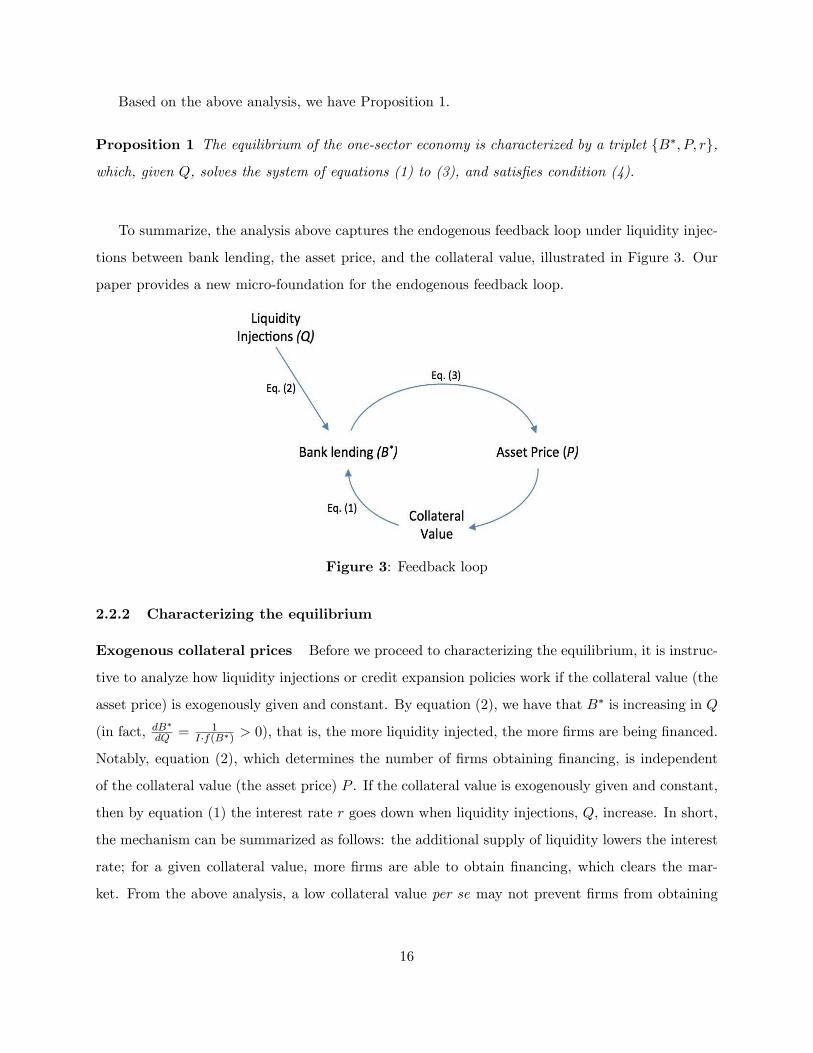
To summarize, the analysis above captures the endogenous feedback loop under liquidity injec-

tions between bank lending, the asset price, and the collateral value, illustrated in Figure 3. Our

paper provides a new micro-foundation for the endogenous feedback loop.

Figure 3: Feedback loop

2.2.2 Characterizing the equilibrium

Exogenous collateral prices Before we proceed to characterizing the equilibrium, it is instruc-

tive to analyze how liquidity injections or credit expansion policies work if the collateral value (the

asset price) is exogenously given and constant. By equation (2), we have that B� is increasing in Q

(in fact, dB�

dQ = 1I�f(B�) > 0), that is, the more liquidity injected, the more �rms are being �nanced.

Notably, equation (2), which determines the number of �rms obtaining �nancing, is independent

of the collateral value (the asset price) P . If the collateral value is exogenously given and constant,

then by equation (1) the interest rate r goes down when liquidity injections, Q, increase. In short,

the mechanism can be summarized as follows: the additional supply of liquidity lowers the interest

rate; for a given collateral value, more �rms are able to obtain �nancing, which clears the mar-

ket. From the above analysis, a low collateral value per se may not prevent �rms from obtaining

16

�nancing under liquidity injections, because an even lower interest rate can channel lending to

�rms.30

In our model, the collateral value (the asset price) is endogenous to liquidity injections and the

equilibrium interest rate may be non-monotonic in liquidity injections. We are interested in the

answers to the following comparative static questions: What is the e¤ect of liquidity injections on

the equilibrium asset price and the equilibrium interest rate (i.e., the functions P (Q) and r (Q))?

What is the role of asset speci�city in the e¤ect?

First, we examine how liquidity injections impact the asset price P . Intuitively, liquidity injec-

tions enable more �rms to make their liquidity investment at T0 and hence increase the liquidity

in the industry at T1, which in turn may raise the equilibrium asset price.

Formally, we can prove that � in (3) is an increasing function of Q. In fact, from (2), B� is

increasing in Q. We can also obtain that the total derivative d�dB� is positive if C � I (1 + r) > 0.

Therefore, under this condition, � is certainly increasing in B� and thus in Q.

Lemma 1 The equilibrium price � is increasing in Q if C � I(1 + r) > 0 in equilibrium.

Proof: See the Appendix.

The intuition for Lemma 1 is the following. Liquidity injections Q enable more �rms, which are

otherwise unable, to make the liquidity investment. Suppose in the economy there is one more �rm

switching from non-investing to investing at T0. Given r, this increases the liquidity in the sector at

T1 by an amount C� I (1 + r), which corresponds to the NPV of the marginal investment in (4).31

More liquidity in the sector (industry) at T1 increases the asset price, in the spirit of Shleifer and

Vishny (1992). We show that the condition in Lemma 1, which is also condition (4) in Proposition

1, holds under general parameter values and hence � is increasing in Q.

Crucially, we need to consider the lower bound of P in (3). The asset speci�city plays an

important role here. If X is low, the buyers cannot leverage much when buying. Hence, the asset

30Benmelech and Bergman (2012) and others study credit traps, where the interest rate may hit zero bound. Our

paper has a di¤erent focus.31There is a further general equilibrium e¤ect because r changes. We prove that the overall e¤ect is positive when

C � I (1 + r) > 0. See the proof of Lemma 1 in the Appendix.

17

price is low. It is possible that X is so low that the asset price is trapped at the lower bound EL(ex)no matter what Q (2 [0; Q]) is; that is, P does not change with Q.

We have Proposition 2.

Proposition 2 If X � X, where X is a (positive) cuto¤, the equilibrium asset price P (Q) is a

constant, equal to EL(ex), no matter what the size of the liquidity injection Q (2 [0; Q]) is. If

X > X, P (Q) is (weakly) increasing in Q under general parameter values.32


In Proposition 2, asset speci�city plays an important role in determining the asset price. The

reason is that asset speci�city determines the leverage level of buyers (i.e., the amount of margin

�nancing buyers can access) and thus in�uences the total liquidity available for purchases and thus

the asset price. Proposition 2 gives the cleanest case for liquidity injections having little impact

on the asset price.33 This happens when the �nancing friction is su¢ ciently high (X su¢ ciently

low).34

Margin levels can di¤er substantially across sectors. For example, the margin level for purchas-

ing �nancial assets including real estate can be signi�cant, while the margin level for purchasing

real assets like equipment or machines can be negligible. On the eve of the 2007-2009 �nancial

crisis, the haircut in trading mortgage-backed security (MBS) often amounted to less than 10%,

or the margin level in terms of the debt-to-asset ratio equated to above 90%; the margin level for

trading stocks is typically around 50% (see Gorton and Metrick (2010) and Adrian and Shin (2010)

for evidence on margins). Di¤erent margin levels across industries clearly give cross-sectional asset

price implications.35

32For our purpose, we focus on the set of equilibria in which � is lower than and not binding at EH(ex). This canbe achieved by assuming that �H and thus EH(ex) are su¢ ciently big, ceteris paribus.33For the bene�t of a clean analysis and for our purpose, we have divided X into two regions in the analysis:

X � X and X > X. The merit of the cleanness can be further seen later when we discuss Figures 4a and 4b. The

results of the paper however hold generally (for some Q).34 In this sense, buyers� internal funds and external funds are complementary in purchasing assets; more internal

funds push up the asset price only when the external funds are above a threshold.35See, e.g., Garleanu and Pedersen (2011) and Frazzini and Pedersen (2011) for evidence on margin-based asset

pricing.

18

That the asset price can be pegged to the valuation under low beliefs has empirical support.

In fact, in an economic downturn, agents are often quite uncertain about economic prospects.

In particular, in the aggregate, agents appear to be acting as if under �Knightian uncertainty�

(i.e., agents use a worst-case for the uncertain probabilities in valuations, see, e.g., Caballero and

Krishnamurthy (2008)), and asset prices are depressed and exhibit features of ��ight to quality�

phenomena. Those times may correspond to � being low in our model, in which case margin levels

can be crucial in determining how asset prices respond to liquidity injections.

In light of the earlier discussion, a low collateral value per se may not prevent �rms from

obtaining �nancing under liquidity injections, as an even lower interest rate can channel lending

to �rms. What matters in our model is that liquidity injections may have asymmetric impacts on

collateral prices across the two sectors (with di¤erent Xs), which can generate the crowding-out

e¤ect.

Next, we examine the response of the equilibrium interest rate to the liquidity injection. On

the one hand, liquidity injections translate into additional supply of loans. On the other hand,

liquidity injections may raise the asset price and thus the collateral value (for bank loans); the

higher collateral value means that more �rms can borrow and compete for loans. That is, the

e¤ective demand for liquidity increases. As a result of the simultaneous increase in both the supply

of and the demand for liquidity, the equilibrium interest rate can either go up or down.

Formally, from the optimal lending condition (1), we have the equilibrium interest rate as

r = P (Q)B�(Q) � 1, where P (Q) has the properties of Proposition 2 and B

�(Q) is uniquely determined

by market clearing (2). We also have that B�(Q) is increasing in Q. Therefore, if P (Q) is constant,

then r is certainly decreasing in Q. If P (Q) is increasing in Q, it is ambiguous whether r is

decreasing or increasing in Q. Indeed, we prove that r can go in either direction depending on

whether P (Q) increases faster or slower than B�(Q). Also, we have the following result: when

Q is very low (close to 0), r is generally decreasing in Q. To see the intuition, we consider the

equilibrium interest rate when Q = 0; in this case, all bank loans are �inside liquidity�and no cash

�ow at T1 is used to repay the interest on �outside liquidity�Q, and hence the asset price relative

to the threshold B� (that is, P (Q)B�(Q) jQ=0) is high; when Q increases away from zero, a part of the

cash �ow at T1 starts to be repaid as the interest on �outside liquidity�, and henceP (Q)B�(Q) decreases.

19

Proposition 3 summarizes the relationship between r and Q.

Proposition 3 If the �nancing friction is high, X � X, the equilibrium interest rate r(Q) is

strictly decreasing in Q (2 [0; Q]). For lower �nancing frictions, X > X, under some distribution

f(B) and some parameters, r(Q) decreases �rst and then increases in Q, that is, there exists a

minimum r(Q), denoted rmin, for an interior Q 2 (0; Q).


The interest rate equilibrates the (e¤ective) demand for liquidity, captured by the collateral

value (asset price) P , and the supply of liquidity, captured by the threshold B�, through 1 + r =P (Q)B�(Q) . Proposition 3 delineates two important cases. First, if the asset price is constant, then the

interest rate certainly decreases in liquidity injections because the supply of loans increases with

liquidity injections. Second, the asset price may increase very fast, faster than B�. In this case, the

interest rate increases with liquidity injections. In fact, the latter case happens when the density

f(B) is thick in some region of B. Note that dB�

dQ = 1I�f(B�) . If the density of f(B

�) is high, B�

increases very slowly in Q, not as fast as P (Q) does, hence the interest rate increases.

Remark We can explain the above mechanisms in the framework of the demand and supply

equilibrium. When more liquidity is injected, which is on the supply side, the interest rate typically

falls. However, in the model, the supply may also in�uence the demand. Additional liquidity

injected may push up the asset price and thus the collateral value; hence the e¤ective demand for

liquidity also increases. When the increase in the e¤ective demand is greater than the increase in

supply, the interest rate goes up rather than down.

Figures 4a and 4b illustrate the equilibrium interest rate under the demand and supply equi-

librium. The e¤ective demand of liquidity is a decreasing function of the interest rate (for a given

collateral value), i.e., the higher the interest rate, the lower the demand. Thus, the additional

supply of liquidity typically causes the equilibrium interest rate to fall, which is the case of Figure

4a. However, in general equilibrium, the supply may also change the e¤ective demand, i.e., the

e¤ective demand curve shifts upward because the collateral value increases. The demand curve

may move upward very fast, and hence the equilibrium interest rate is non-monotonic in liquidity

supply, which is the case of Figure 4b. Formally, in our model, the aggregate supply of liquidity is

20

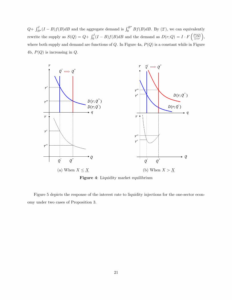
Q+R IB�(I �B)f(B)dB and the aggregate demand is

R B�0 Bf(B)dB. By (2�), we can equivalently

rewrite the supply as S(Q) = Q+R I0 (I � B)f(B)dB and the demand as D(r;Q) = I � F

�P (Q)1+r

�,

where both supply and demand are functions of Q. In Figure 4a, P (Q) is a constant while in Figure

4b, P (Q) is increasing in Q.

(a) When X � X (b) When X > X

Figure 4: Liquidity market equilibrium

Figure 5 depicts the response of the interest rate to liquidity injections for the one-sector econ-

omy under two cases of Proposition 3.

21

Figure 5: The response of the interest rate to liquidity injections for the one-sector economy

2.3 Two-sector economy

In this subsection, we analyze the economy with two sectors: Sector 1 and Sector 2. We study

the distribution of liquidity in the economy and the distribution�s e¤ect on aggregate economic

performance. We �rst solve for the two-sector equilibrium to highlight the crowding-out e¤ect, and

then consider the optimal decision of the central bank and analyze the welfare implications of the

model.

2.3.1 Two-sector equilibrium: the crowding-out e¤ect

In order to highlight the key mechanism underlying the crowding-out e¤ect, at this stage we assume

that the two sectors di¤er only in their asset speci�city. That is, we assume that the cash �ow of the

project, the internal capital distribution of �rms, and all other aspects are identical across the two

sectors. The only di¤erence is that the two sectors have di¤erent Xs, the contractible part of the

cash �ow at T2. Sector 1 has a higher friction, a lower X denoted X1, where X1 � X, while Sector

2 has a lower friction, a higher X denoted X2, where X2 > X.36 Note that X determines asset

36For cleanness, we consider that X2 > X � X1. When X2 > X1 � X, the result in this subsection (i.e., the

unique optimal level of liquidity injection as will be shown in Propositions 5 and 7) still holds. However, a stricter

condition is required, that is, the maximum amount of allowed liquidity injection Q cannot be too large. The reason

is that when X2 > X1 > X, the interest rates in both sectors are increasing in the liquidity in�ow when the liquidity

in�ow is su¢ ciently high. Hence, the crowding-out e¤ect occurs only when Q is not very large.

22

leverage while B� measures corporate leverage in a sector; asset leverage (at T1) impacts corporate

leverage (at T0).

The central bank can decide the aggregate liquidity to inject into the economy but cannot

control the allocation of the liquidity across the two sectors in the economy, which is determined

by commercial banks based on market forces. Market forces mean that: 1) commercial banks make

loans only based on �rms�repaying ability or collateral values (no matter which sector �rms are

from) and 2) there is a single interest rate in the economy (for both sectors). Also, the central

bank cannot control the (real) interest rate directly. In fact, central banks generally control only

the overnight interest rate but cannot control long-term real interest rates �the ultimate interest

rates that matter for real businesses (see Blinder (1998, p. 70)); also, in our model, one r may map

into two Qs (i.e., not a one-to-one mapping).

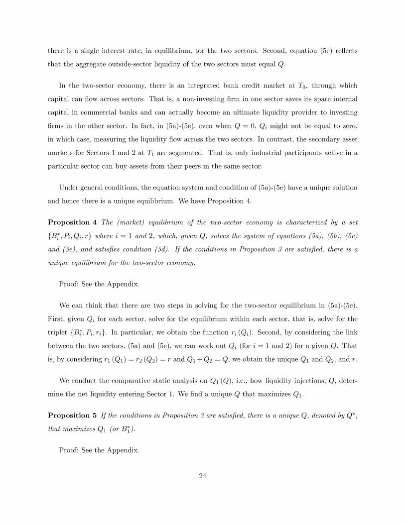
We solve for the two-sector economy equilibrium: for a given Q, how the liquidity is allocated

and distributed across the two sectors. The equilibrium is given by the following equation system

and condition:

r =PiB�i

� 1 (5a)Z I

B�i

(I �B) f (B) dB +Qi =Z B�i

0Bf (B) dB (5b)

Pi = p(ex;B�i ; C;Xi; r) (5c)

C � I(1 + r) � 0 (5d)

Q =Xi

Qi; (5e)

where i = 1 and 2.

In (5a)-(5e), the variables with superscript i denote the variables for sector i, where i = 1 and

2. In particular, Qi is de�ned as the net amount of outside-sector liquidity entering sector i, or the

net liquidity in�ow into sector i. Equations (5a), (5b) and (5c), and condition (5d) correspond, in

order, to the respective equations (1), (2) and (3), and condition (4) of the one-sector economy.

The three equations ((5a) through (5c)) and condition (5d) give the equilibrium within each sector.

The interaction between the two sectors is given by (5a) and (5e). First, equation (5a) states that

23

there is a single interest rate, in equilibrium, for the two sectors. Second, equation (5e) re�ects

that the aggregate outside-sector liquidity of the two sectors must equal Q.

In the two-sector economy, there is an integrated bank credit market at T0, through which

capital can �ow across sectors. That is, a non-investing �rm in one sector saves its spare internal

capital in commercial banks and can actually become an ultimate liquidity provider to investing

�rms in the other sector. In fact, in (5a)-(5e), even when Q = 0, Qi might not be equal to zero,

in which case, measuring the liquidity �ow across the two sectors. In contrast, the secondary asset

markets for Sectors 1 and 2 at T1 are segmented. That is, only industrial participants active in a

particular sector can buy assets from their peers in the same sector.

Under general conditions, the equation system and condition of (5a)-(5e) have a unique solution

and hence there is a unique equilibrium. We have Proposition 4.

Proposition 4 The (market) equilibrium of the two-sector economy is characterized by a set

fB�i ; Pi; Qi; rg where i = 1 and 2, which, given Q, solves the system of equations (5a), (5b), (5c)

and (5e), and satis�es condition (5d). If the conditions in Proposition 3 are satis�ed, there is a

unique equilibrium for the two-sector economy.


We can think that there are two steps in solving for the two-sector equilibrium in (5a)-(5e).

First, given Qi for each sector, solve for the equilibrium within each sector, that is, solve for the

triplet fB�i ; Pi; rig. In particular, we obtain the function ri (Qi). Second, by considering the link

between the two sectors, (5a) and (5e), we can work out Qi (for i = 1 and 2) for a given Q. That

is, by considering r1 (Q1) = r2 (Q2) = r and Q1+Q2 = Q, we obtain the unique Q1 and Q2, and r.

We conduct the comparative static analysis on Q1 (Q), i.e., how liquidity injections, Q, deter-

mine the net liquidity entering Sector 1. We �nd a unique Q that maximizes Q1.

Proposition 5 If the conditions in Proposition 3 are satis�ed, there is a unique Q, denoted by Q�,

that maximizes Q1 (or B�1).


24

Figure 6 depicts the unique Q�. In the �gure, Q� = Q1 +Q2. If the liquidity injection exceeds

this level, all additional liquidity goes to Sector 2 and, further, some liquidity in Sector 1 is actually

squeezed out due to the increased interest rate. Therefore, overall, the liquidity in Sector 2 increases

while that in Sector 1 decreases. In fact, if Q increases above Q�, Sector 1 cannot attract more

liquidity as there is otherwise no interest rate at which the market across the two sectors can clear;

thus Sector 2 must attract more liquidity, which will certainly increase the interest rate as we go

along the increasing portion of the liquidity curve of Sector 2.

Figure 6: Crowding-out e¤ect in the two-sector economy equilibrium

It is important to examine the process by which the new equilibrium is reached when some

additional amount of liquidity (beyond Q�) is injected. In Figure 6, in which an additional amount

of liquidity �Q = (Q01 +Q02) � (Q1 +Q2) is injected, we examine how Q1 reaches Q01. Suppose

initially all additional liquidity, �Q, enters Sector 2; this would push up the interest rate; the higher

interest rate would squeeze some liquidity out of Sector 1, which means that more liquidity would

�ow into Sector 2, pushing up the interest rate further, and so on in a spiral. Essentially, there is

a spiral in reaching the new equilibrium. From the perspective of Sector 2, the spiral results in a

multiplier Q02�Q2�Q > 1; that is, although the (aggregate) additional amount of liquidity injection is

�Q, the increment of liquidity in Sector 2 is actually more than �Q; the leap is at the expense

of liquidity �ows to Sector 1, causing a liquidity drain out of Sector 1. In short, one sector enters

25

a liquidity-asset price �in�ationary�cycle while the other enters a �de�ationary�cycle, and the two

cycles reinforce each other.

In sum, we can divide the support of liquidity injection, Q, into two regions: Q � Q� and

Q > Q�. In the region of Q � Q�, the liquidity in both sectors increases with liquidity injections.

In the region of Q > Q�, additional liquidity injected increases the liquidity in one sector but

reduces that in the other, that is, the �crowding-out�e¤ect occurs. The �crowding-out�occurs in a

spiral. We have Proposition 6.

Proposition 6 When Q � Q�, there is an �allocation�e¤ect, i.e., liquidity in both sectors increases

with liquidity injections but Sector 1 obtains less liquidity than Sector 2. When Q > Q�, there is a

�crowding-out� e¤ect, i.e., more liquidity injected increases the liquidity in Sector 2 but reduces it

in Sector 1; the crowding-out occurs in a self-reinforcing spiral.


Although the investments in the two sectors have the same surplus (i.e., C � I), the liquidity

is unevenly distributed across the two sectors. In particular, if too much liquidity is injected into

the economy, Sector 1 can actually su¤er a liquidity out�ow. As long as the collateral value (the

asset price) in one sector increases faster than that in the other sector, there is the possibility of

crowding out.

2.3.2 The central bank�s decisions and the welfare implications

We model two alternative objective functions of the central bank, which deliver qualitatively equiv-

alent results. That is, there is an optimal level of liquidity injection for the central bank and the

liquidity injection should not be too high. This result is robust under either objective function. The

�rst objective function is that the central bank targets to maximize the number of �rms in Sector

1 that can undertake the liquidity investment. This may be because the government cares more

about outcomes such as employment (e.g., small and medium-sized businesses) than purely �rms�

pro�ts. If Sector 1, relative to Sector 2, is disproportionately more important in these aspects, the

government may make Sector 1 its �rst priority in economic stimulus. In this case, there exists an

26

optimal level of liquidity injection for the central bank, as shown in Proposition 5.37

Second, we assume that the government is to maximize the total surplus in terms of cash �ows

of liquidity investments in the economy. To make the problem interesting and relevant, we assume

that the two sectors di¤er in both their cash �ow at T0 and their asset speci�city while holding

all other aspects same. Speci�cally, we assume that C1 > C2 and X1 < X2, where Ci and Xi are,

respectively, the cash �ow at T1 and the asset speci�city for sector i, and i = 1 and 2. That is,

Sector 1 has a higher cash �ow and higher asset speci�city.

The total surplus of liquidity investments in the economy is then

W =

Z B�1

0(C1 � I)f (B) dB +

Z B�2

0(C2 � I)f (B) dB:

The total surplus W is, in the end, divided among investing �rms (pro�ts), non-investing �rms

(interest on deposits) and the government (interest on Q) (see the proof of Proposition 7 in the

Appendix). We make one remark. In general, it is di¢ cult to conduct welfare analysis on models

with heterogeneous beliefs (see, e.g., Brunnermeier, Simsek and Xiong (2012)). However, this is

not the case with our model. In our model, we assume that the cash �ow ex at T2 (over which �rmsdevelop heterogeneous beliefs) and the distribution of beliefs (i.e., the probability �) are identical

across the two sectors. More importantly, the asset, which generates cash �ow ex, is in place at T0;liquidity injections are irrelevant to it. Liquidity injections only impact the liquidity investment I

and the cash �ow C subsequently. Hence, we can conduct the welfare analysis of liquidity injections

by calculating how many �rms undertake the liquidity investment to realize the positive surplus

C � I, which is how W is calculated in our model.

37 In terms of modelling, we can assume that the liquidity investment for �rms in Sector 1 generates not only cash

�ow C but also some non-pecuniary payo¤s.

27

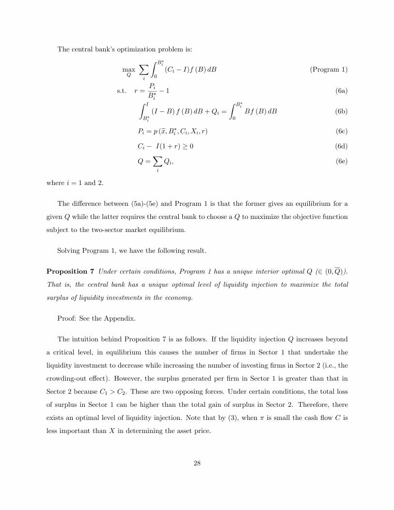
The central bank�s optimization problem is:

maxQ

Xi

Z B�i

0(Ci � I)f (B) dB (Program 1)

s.t. r =PiB�i

� 1 (6a)Z I

B�i

(I �B) f (B) dB +Qi =Z B�i

0Bf (B) dB (6b)

Pi = p (ex;B�i ; Ci; Xi; r) (6c)

Ci � I(1 + r) � 0 (6d)

Q =Xi

Qi; (6e)

where i = 1 and 2.

The di¤erence between (5a)-(5e) and Program 1 is that the former gives an equilibrium for a

given Q while the latter requires the central bank to choose a Q to maximize the objective function

subject to the two-sector market equilibrium.

Solving Program 1, we have the following result.

Proposition 7 Under certain conditions, Program 1 has a unique interior optimal Q (2 (0; Q)).

That is, the central bank has a unique optimal level of liquidity injection to maximize the total

surplus of liquidity investments in the economy.


The intuition behind Proposition 7 is as follows. If the liquidity injection Q increases beyond

a critical level, in equilibrium this causes the number of �rms in Sector 1 that undertake the

liquidity investment to decrease while increasing the number of investing �rms in Sector 2 (i.e., the

crowding-out e¤ect). However, the surplus generated per �rm in Sector 1 is greater than that in

Sector 2 because C1 > C2. These are two opposing forces. Under certain conditions, the total loss

of surplus in Sector 1 can be higher than the total gain of surplus in Sector 2. Therefore, there

exists an optimal level of liquidity injection. Note that by (3), when � is small the cash �ow C is

less important than X in determining the asset price.

28

Under either objective function of the central bank, we draw the same conclusion that the level

of liquidity injection should not be too high. In fact, the key underlying mechanism for the optimal

liquidity injection under either objective function is the crowding-out e¤ect.

Program 1 also corresponds to the constrained second best equilibrium of the two-sector economy.

In this equilibrium, the social planner (the government) decides the optimal Q by taking account of

the incentives of the private sector (i.e., the constraints of (6a)-(6e)). If liquidity injections exceed

the constrained optimal level, not only are investments in Sector 1 crowded out but also the total

surplus in terms of cash �ows in the economy is reduced. In this sense, excessive liquidity injections

lead to a misallocation of liquidity in the economy: lower-surplus projects obtain more liquidity

while higher-surplus projects lose liquidity such that the total surplus in the economy is reduced.

This gives the welfare (e¢ ciency) implication of the model.

Corollary 1 If liquidity injections exceed the constrained optimal level given by Program 1, there

is a misallocation of liquidity in the economy.

3 Empirical implications

We have shown that if too much liquidity is injected into the economy, there is the possibility of

crowding-out across sectors. In this section, we intend to understand under what circumstances

crowding-out is more likely to occur and what its implication is for the optimal liquidity injection.

We derive two implications, a cross-sectional one and one in the time series.

We �rst analyze the cross-sectional implication. Recall that the term X measures the con-

tractible part of the project payo¤, which depends on the project�s asset speci�city. We expect

that the cross-country di¤erence in payo¤ contractibility is small for industries with low asset

speci�city while the cross-country di¤erence is larger for industries with higher asset speci�city.

For example, the leverage (margin) level in the real estate sector may not vary much across coun-

tries while the leverage level in the real sector (e.g., trading machines and equipment) can di¤er

signi�cantly across countries. This is similar to the phenomenon that the degree of external �-

nance dependence in industries with higher asset tangibility is similar across countries while that

in industries with lower asset tangibility varies largely across countries. In fact, for a country with

poorer contracting institutions, creditors can realize a lower fraction of the investment payo¤ in

29

case of default if asset tangibility is low (see, e.g., La Porta et al. (1997, 1998), Djankov et al.

(2008), Almeida and Campello (2007)). This can be due to an ine¢ ciency of contract enforcement

or high transaction costs in �nancial markets in liquidating collateral. Speci�cally, holding X2

(the contractible part of the project payo¤ for Sector 2 with lower asset speci�city) similar for all

countries, we expect X1 (the contractible part of the project payo¤ for Sector 1 with higher asset

speci�city) to be lower for a country with poorer contacting institutions.

By conducting a comparative statics analysis on two countries with a similar X2 but di¤erent

levels of X1, we have the following prediction.

Implication 1 (Cross-sectional implication) For a country with poorer contracting institu-

tions, the crowding-out occurs under a wider range of Q and the optimal level of liquidity injection

is lower.


As for the time-series implication, our main interest is in the uncertainty about economic

prospects. Speci�cally, consider a mean-preserving spread of �L and �H , that is, hold the average

of �L and �H constant while increasing their distance, �H��L. Then, the distance �H��L measures

the degree of divergence in investors�opinions. We can characterize the uncertainty about economic

prospects by the degree of divergence in opinions. The higher the degree of divergence, the higher

the uncertainty about economic prospects. We have Implication 2.

Implication 2 (Time-series implication) At a time of higher uncertainty about economic

prospects, the crowding-out occurs under a wider range of Q and the optimal level of liquidity

injection is lower.


The intuition behind Implication 2 is as follows. We consider a pair (�0L,�0H), which is a mean-

preserving spread of the pair (�L,�H), that is, �0L < �L < �H < �0H . Under the mean-preserving

spread, the lower bound of the asset price decreases, that is, E�0L(ex) < E�L(ex). For Sector 1, if its

original asset price binds at the lower bound E�L(ex), the divergence of opinion reduces the assetprice. In contrast, for Sector 2, under the divergence of opinion, the asset price remains unchanged

for the range of high Q. Therefore, the gap in asset prices between the two sectors widens. As

30

a result, the optimal level of liquidity injection is lower. Hence, for a given Q, the crowding-out

occurs more likely under higher uncertainty.

4 Conclusion

The paper studies why economic stimulus by way of liquidity injections (credit easing) may not

work. We highlight the friction of imperfect �nancial contracting. We show that there is feedback

between liquidity injections and �rm asset collateral values in an economy. This feedback, however,

is asymmetric across sectors. The sector with lower friction has stronger feedback. This asymmetry

creates a crowding-out e¤ect. For the sector with lower friction, the collateral value responds

strongly to liquidity injections, which can push up the interest rate; the increased interest rate

reduces the liquidity in the sector with higher friction as the collateral value in that sector responds

feebly. Therefore, even if the collateral value in one sector increases with liquidity injections, as

long as the increase is not as fast as that in the other sector, there is the possibility of crowding

out, which holds back economic recovery.

Our paper has two empirical implications. The model implies that crowding-out is more likely in

a country with poorer contracting institutions and at a time of greater uncertainty about economic

prospects. Authorities should be more cautious about the crowding-out e¤ect in these situations.

The paper highlights limitations of (unconventional) monetary policy in stimulating economic

growth. While �nancial intermediaries have an (informational) advantage/expertise in allocating

capital to �rms, the market frictions also mean that implementation of monetary policy through

�nancial intermediaries is not perfect. The paper implies that monetary policy in conjunction

with �scal policy to target some speci�c sectors/industries might have better e¤ects in economic

stimulus. Regulation on the leverage level in more speculative industries when other industries are

in distress might be helpful in reducing the crowding-out e¤ect.

31

5 References

Acharya, Viral and S. Viswanathan, 2011, �Leverage, Moral Hazard and Liquidity,� Journal of

Finance 66: 1, 99�138.

Adrian, Tobias and Hyun Song Shin (2010), �Liquidity and Leverage,� Journal of Financial

Intermediation, 19, 3, 418-437.

Allen, Franklin and Douglas Gale, 2000, �Bubbles and Crises,� The Economic Journal 110,

(2000), 236-255.

Almeida, Heitor and Murillo Campello, 2007, �Financial Constraints, Asset Tangibility and

Corporate Investment,�Review of Financial Studies 20: 1429-1460.

Benmelech, Efraim, 2009, �Asset Salability and Debt Maturity: Evidence from 19th Century

American Railroads,�Review of Financial Studies, 22(4), 1545�1583.

Benmelech, Efraim and Nittai Bergman, 2009, �Collateral Pricing,�Journal of Financial Eco-

nomics, 91(3) 339-360.

� � , 2011, �Bankruptcy and the Collateral Channel,�The Journal of Finance, 66(2), 337�378.

� � , 2012, �Credit Traps,�American Economic Review, 102(6): 3004-32.

Bernanke, Ben and Mark Gertler, 1989, �Agency Costs, Net Worth, and Business Fluctuations,�

American Economic Review 79 (1989) 14-31.

� � , 1995, �Inside the Black Box: The Credit Channel of Monetary Policy Transmission,�

Journal of Economic Perspectives 9, 27-48.

Blanchard, Olivier, 2008, �Crowding out,�The New Palgrave Dictionary of Economics, 2nd Ed.

Blinder, Alan, 1998, �Central Banking in Theory and Practice,�MIT Press, Cambridge.

Brunnermeier, Markus, Thomas Eisenbach and Yuliy Sannikov (2013), �Macroeconomics with

Financial Frictions: A Survey,�Advances in Economics and Econometrics, Tenth World Congress

of the Econometric Society, New York.

Brunnermeier, Markus, and Alp Simsek and Wei Xiong (2012), �A Welfare Criterion for Models

with Distorted Beliefs,�working paper, Princeton University ant MIT.

Caballero, Ricardo and Arvind Krishnamurthy, 2008, �Collective Risk Management in a Flight

to Quality Episode,�Journal of Finance, vol. 63(5), 2195-2230.

Chakraborty, Indraneel, Itay Goldstein and Andrew MacKinlay, 2013, �Do Asset Price Bubbles

have Negative Real E¤ects?�Working paper, University of Pennsylvania.

32

Diamond, Douglas and Raghuram Rajan, 2002, �Bank Bailouts and Aggregate Liquidity,�

American Economic Review 92(2), 38-41.

� � , 2006, �Money in a Theory of Banking,�American Economic Review 96(1), 30-53.

Djankov, Simeon, Oliver Hart, Caralee McLiesh, Andrei Shleifer, 2008, �Debt Enforcement

around the World�, Journal of Political Economy, 2008, vol. 116.

Frazzini, Andrea and Lasse Heje Pedersen, 2011, �Embedded Leverage,�working paper, NYU.

Garleanu, Nicolae and Lasse Heje Pedersen, �Margin-Based Asset Pricing and Deviations from

the Law of One Price,� The Review of Financial Studies, 24(6), 1980-2022.

Geanakoplos, John, 2010, �The Leverage Cycle�, NBER Macro Annual, pp1-65.

Gertler, Mark and Peter Karadi, 2011, �A Model of Unconventional Monetary Policy,�Journal

of Monetary Economics 58 (2011), 17-34.

Gertler, Mark and Nobuhiro Kiyotaki, 2010, �Financial Intermediation and Credit Policy in

Business Cycle Analysis,�Handbook of Monetary Economics.

Gilchrist, Simon and Egon Zakrajsek, 2013, �The Impact of the Federal Reserve�s Large-Scale

Asset Purchase Programs on Default Risk�, NBER Working Paper No. 19337.

Harrison, Michael and David Kreps, 1978, �Speculative Investor Behavior in a Stock Market

with Heterogeneous Expectations,�Quarterly Journal of Economics, 92, p.323-36.

Hart, Oliver and John Moore, 1994, �A Theory of Debt Based on the Inalienability of Human

Capital,�Quarterly Journal of Economics 109, 841-79.

� � , 1998, �Default and Renegotiation: A Dynamic Model of Debt,� Quarterly Journal of

Economics 113(1), 1-41.

Holmstrom, Bengt and Jean Tirole, 1997, �Financial Intermediation, Loanable Funds, and the

Real Sector,�Quarterly Journal of Economics 112(3), 663-691.

Kalemli-Ozcan, Sebnem, Bent Sorensen and Sevcan Yesitas, 2011, �Leverage across Firms,

Banks and Countries,�Working paper, University of Houston.

Kiyotaki, Nobuhiro and John Moore, 1997, �Credit Cycles,�Journal of Political Economy 105

(2): 211�248.

� � , 2002, �Evil is the Root of All Money,�American Economic Review: Papers and Proceed-

ings, 85 (2002), 62-66.

Krishnamurthy, Arvind and Annette Vissing-Jorgensen, 2011, �The E¤ects of Quantitative

Easing on Interest Rates: Channels and Implications for Policy,�Brookings Papers on Economic

33

Activity.

LaPorta, Rafael, Florencio Lopez-de-Silanes, Andrei Shleifer and Robert Vishny, 1997, �Legal

Determinants of External Finance,�Journal of Finance 52 (July): 1131�50.

� � ,1998, �Law and Finance,�Journal of Political Economy, 106 (December): 1113�55.

Mendoza, Enrique, 2010, �Sudden Stops, Financial Crises and Leverage,�American Economic

Review, 100, 1941-66.

Miller, Edward, 1977, �Risk, Uncertainty, and Divergence of Opinion,�Journal of Finance, Vol.

32, No. 4, p.1151-1168.

Rajan, Raghuram, 1992, �Insiders and Outsiders: The Choice between Informed and Arm�s-

Length Debt,�The Journal of Finance, Vol. 47, No. 4, pp. 1367-1400.

Reinhart, Carmen and Graciela Kaminsky, 1999, �The Twin Crises: The Causes of Banking

and Balance-of-Payments Problems,�American Economic Review, vol. 89(3), 473-500.

Reis, Ricardo, 2009, �Interpreting the Unconventional U.S. Monetary Policy of 2007-09,�Brook-

ings Papers on Economic Activity, 40, 119-165.

� � , 2014, Discussions on Maurice Obstfeld�s �Finance at Center Stage: Some Lessons of the

Euro Crisis�in the session of Teaching the Euro Crisis, the AEA meetings in Philadelphia.

Shleifer, Andrei, and Robert W. Vishny, 1992, �Liquidation Values and Debt Capacity: A

Market Equilibrium Approach,�Journal of Finance 47, 143-66.

� � , 2010a, �Unstable Banking�, Journal of Financial Economics, 97, 306�318.

� � , 2010b, �Asset Fire Sales and Credit Easing,�American Economic Review, 100(2), 46-50.

� � , 2011, �Fire Sales in Finance and Macroeconomics,� Journal of Economic Perspectives,

25(1), 29-48.

Simsek, Alp, 2012, �Belief Disagreements and Collateral Constraints,�Econometrica, forthcom-

ing.

Tirole, Jean, 1985, �Asset Bubbles and Overlapping Generations,�Econometrica 53, pp. 1499-

1528.

Williamson, Oliver, 1985, �The Economic Institutions of Capitalism,�Free Press, NY, 1985.

� � , 1986, �Economic Organization: Firms, Markets, and Policy Control,�New York Univer-

sity Press, NY, 1986.

� � , 1988, �Corporate Finance and Corporate Governance,�Journal of Finance 43, 567-91.

34

6 Appendix

A numerical example:

We provide a numerical example for the crowding-out e¤ect, illustrating the existence of relevant

parameters in the propositions. That is, the numerical example is to highlight the qualitative (rather

than quantitative) aspect of the model.

We choose parameter values as simple as possible. We set the parameter values for the project

as I = 1, C = 2:2, � = 0:4, EH(ex) = 1:3668, EL(ex) = 1:0334. Note that we do not need to specifyexactly u, d, �H and �L, any combination of which that satis�es that u > d > 0, 0 � X1 < X2 � d,

u � �H + d � (1 � �H) = 1:3668 and u � �L + d � (1 � �L) = 1:0334 works. The �rm distribution is

f(B) = log 11�B for B 2 [0; 1). As the maximum total amount of liquidity that any one sector can

demand is Qmax =R 10 Bf(B)dB = 0:75, we set Q = 2Q

max = 1:5.

Given that EL(ex) = 1:0334, we can calculate the threshold X in Proposition 1, which is

X = 0:0501. We set X1 = 0:05 and X2 = 0:35, where X1 < X < X2.

For Sector 1, we can work out that the asset price is P1 = 1:0334 for any Q1 2 [0; 0:75]. The

asset price is trapped at EL(ex) = 1:0334. The interest rate r1(Q1) is a strictly decreasing functionof liquidity in�ow Q1.

For Sector 2, the asset price P2(Q2) is (weakly) increasing in Q2. When Q2 is small, liquidity

injections are not su¢ cient to push the asset price above EL(ex) and the asset price is P2 = 1:0334;when Q2 is big enough, P2(Q2) is strictly increasing in Q2, with the maximum asset price being

P2(Q2 = 0:75) = 1:3667 (which is lower than EH(ex) = 1:3668). As for the equilibrium interest rate

r2(Q2), it is non-monotonic and �U�-shaped, with the minimum interest rate being rmin = 0:3270.

The optimal amount of liquidity injection to maximize liquidity investments in Sector 1 is

Q� = 0:6113, at which the distribution of the liquidity injection across the two sectors isQ�1 = 0:4163

and Q�2 = 0:1950, respectively.

Figure A1(a) shows the asset price response in each sector to its (net) liquidity in�ow Qi and

Figure A1(b) depicts the interest rate response in each sector.

35

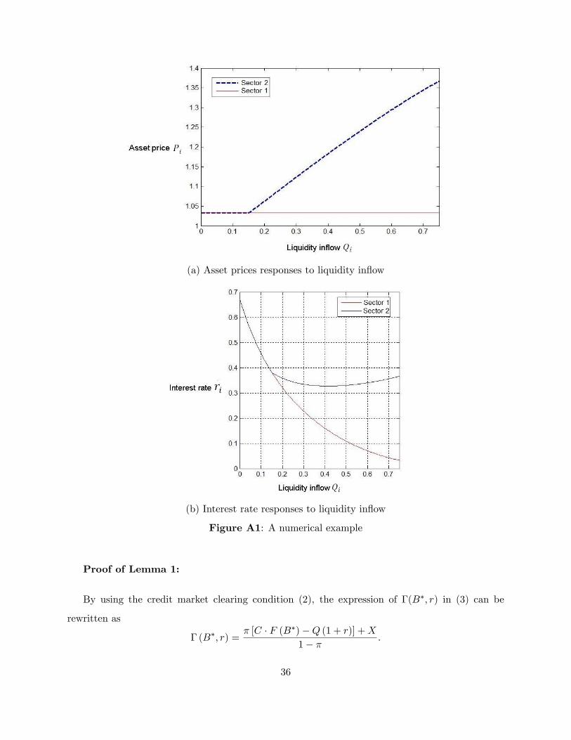
(a) Asset prices responses to liquidity in�ow

(b) Interest rate responses to liquidity in�ow

Figure A1: A numerical example

Proof of Lemma 1:

By using the credit market clearing condition (2), the expression of �(B�; r) in (3) can be

rewritten as

� (B�; r) =� [C � F (B�)�Q (1 + r)] +X

1� � :

36

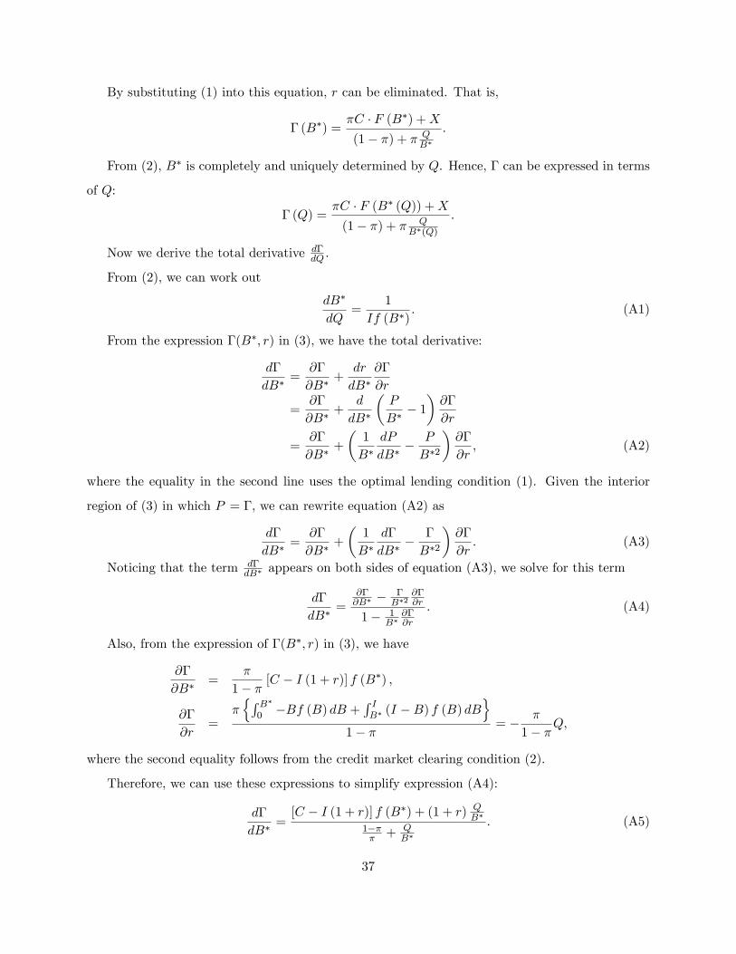
By substituting (1) into this equation, r can be eliminated. That is,

� (B�) =�C � F (B�) +X(1� �) + � Q

B�

:

From (2), B� is completely and uniquely determined by Q. Hence, � can be expressed in terms

of Q:

� (Q) =�C � F (B� (Q)) +X(1� �) + � Q

B�(Q)

:

Now we derive the total derivative d�dQ .

From (2), we can work out

dB�

dQ=

1

If (B�): (A1)

From the expression �(B�; r) in (3), we have the total derivative:

d�

dB�=@�

@B�+dr

dB�@�

@r

=@�

@B�+

d

dB�

�P

B�� 1�@�

@r

=@�

@B�+

�1

B�dP

dB�� P

B�2

�@�

@r; (A2)

where the equality in the second line uses the optimal lending condition (1). Given the interior

region of (3) in which P = �, we can rewrite equation (A2) as

d�

dB�=@�

@B�+

�1

B�d�

dB��

B�2

�@�

@r: (A3)

Noticing that the term d�dB� appears on both sides of equation (A3), we solve for this term

d�

dB�=

@�@B� �

�B�2

@�@r

1� 1B�

@�@r

: (A4)

Also, from the expression of �(B�; r) in (3), we have

@�

@B�=

�

1� � [C � I (1 + r)] f (B�) ;

@�

@r=

�nR B�

0 �Bf (B) dB +R IB� (I �B) f (B) dB

o1� � = � �

1� �Q;

where the second equality follows from the credit market clearing condition (2).

Therefore, we can use these expressions to simplify expression (A4):

d�

dB�=[C � I (1 + r)] f (B�) + (1 + r) QB�

1�� + Q

B�

: (A5)

37

Overall, we have

d�

dQ=dB�

dQ

d�

dB�=[C � I (1 + r)] f (B�) + (1 + r) QB�

If (B�)�1�� + Q

B�

� : (A6)

By (A6), we conclude that a su¢ cient condition for d�dQ > 0 is C � I(1 + r) > 0.

In fact, if drdB� is positive, we immediately conclude that � must increase in Q because � =

B� (1 + r) by (1) and B� is increasing in Q. If drdB� is negative, clearly [C � I (1 + r)] f (B

�) �drdB�Q > 0, meaning d�

dQ > 0. In short, if C � I(1 + r) is positive and close to zero, drdB� must be

negative; if drdB� is positive, C � I (1 + r) must be far above zero and exceed the e¤ect of

drdB� .

Proof of Proposition 2:

For ease of exposition, we reiterate the equilibrium asset price here. That is

P =

8>>>>><>>>>>:EH (ex) if � (B�; r) > EH (ex)� (B�; r) if � (B�; r) 2

�EL (ex) ; EH (ex)� ;

EL (ex) if � (B�; r) < EL (ex)where

� (B�; r) =�hR B�0 [C �B (1 + r)] f (B) dB +

R IB� (1 + r) (I �B) f (B) dB

i+X

1� � :

From Lemma 1, we know that �(Q) is an increasing function of Q if C� I(1+ r) > 0. We show

that the condition C�I(1+r) > 0 holds under general parameter values. In fact, by 1+r = �(B�;r)B� ,

we have C� I(1+ r) = C� I �(B�;r)

B� , where B� is completely determined by Q and r is endogenous.

Ceteris paribus, if � is su¢ ciently low, � is low and thus C � I(1+ r) > 0. The numerical example

above in the Appendix is one case.

We consider the lower bound of the asset price, EL(ex). For our purpose, we choose the para-meters to make sure that the upper bound of the asset price is not binding (i.e., the asset price

calculated in �(Q) is always below EH(ex)). We de�ne two cuto¤s, X and X, and divide X into

three ranges: X < X, X > X, and X � X � X.

38

The �rst range of X is the case in which the asset price is trapped at the lower bound no matter

what Q (2 [0; Q]) is. That is, even if Q = Q, the asset price calculated in � is still (weakly) below

EL(ex). Therefore, X satis�es EL(ex) = �jQ=Q, X=X .The third range of X is the case in which the asset price is above the lower bound for the whole

region of Q 2 [0; Q]. That is, even if Q = 0, the asset price calculated in � is still (weakly) above

EL(ex). Therefore, X satis�es EL(ex) = �jQ=0, X=X .In the second range of X � X � X, the asset price is the constant EL(ex) when Q is low and

then increases in Q when Q is higher.


When X � X, the asset price P is constant in Q. Also considering dB�

dQ > 0, we have that when

X � X, the equilibrium interest rate r(Q) is strictly decreasing in Q (2 [0; Q]).

We consider the equilibrium interest rate when X > X. By r = �B� � 1, we have

dr

dB�=

1

B�d�

dB��

B�2: (A7)

Plugging (A5) into (A7), we have

dr

dB�=[C � I (1 + r)] f (B�)B� � 1��

� ��1�� B� +Q

�B�

: (A8)

By 1 + r = P (Q)B�(Q) , considering P = �, we have

dr

dQ=dB�

dQ

dr

dB�

=1

If (B�)

[C � I (1 + r)] f (B�)B� � 1��

1�� B� +Q

�B�

=[C � I (1 + r)]B� � 1��

��

f(B�)�1�� B� +Q

�B�I

: (A9)

Hence, drdQ > 0 if and only if f(B�) > 1��

�

hC1+r � I

i�1by noting that �

B� = 1+r. In equilibrium,

we guarantee that C > I(1+r), so the right-hand side of this condition is bounded. When f(B�) is

su¢ ciently high (respectively low), drdQ is positive (respectively negative). The numerical example

above in the Appendix illustrates these.

39

We also consider the special case of P (Q)B�(Q) jQ=0. In this case, B

� solvesR IB� (I �B) f (B) dB =R B�

0 Bf (B) dB by noting that B� has a unique solution based on (2�), and � = �C�F (B�)+X1�� . Hence,

r is determined.

To summarize, when X > X, we can choose some function f (B) (i.e., f(B) is su¢ ciently high

in some region of B) and some Q such that r decreases �rst and then increases in Q within the

interval Q 2�0; Q

�.


First, given a Qi for each sector, solve for the equilibrium within each sector, that is, solve for

the triplet fB�i ; Pi; rig. In particular, we obtain the function ri (Qi). If conditions in Proposition

3 are satis�ed, r1 (Q1) is a decreasing function and r2 (Q2) is a �U�-shaped function. Second, by

considering the link between the two sectors, (5a) and (5e), we can work out Qi (for i = 1 and

2) for a given Q. That is, by considering r1 (Q1) = r2 (Q2) = r and Q1 + Q2 = Q, we obtain the

unique Q1 and Q2, and r. In fact, by aggregating r1 (Q1) and r2 (Q2), we can obtain an �aggregate�

function r(Q). That is, for a given r, we �nd the corresponding Q1 which solves r1 (Q1) = r and

Q2 which solves r2(Q2) = r, and then aggregate Q1 and Q2 as Q = Q1 + Q2. Under generally

chosen parameters, the �aggregate�function r(Q) is a �U�-shaped function. The numerical example

above in the Appendix is one case. Thus, for a given Q, we have unique Q1, Q2 and r.


From the proof of Proposition 4, we have that the �aggregate� function r(Q) is a �U�-shaped

function (i.e., decreasing �rst and then increasing). By Proposition 3, r1 (Q1) is a decreasing

function. Therefore, to maximize Q1, we need to choose a Q to minimize r(Q). Clearly, there is a

unique Q that minimizes r and thus maximizes Q1.


Considering that r1 (Q1) is a decreasing function and r2 (Q2) is a �U�-shaped function, we �nd

a unique Q�1 that solves r1 (Q�1) = rmin and a unique Q�2 that solves r2 (Q

�2) = rmin. We de�ne

Q� = Q�1 + Q�2. By r1 (Q1) = r2 (Q2) = r and Q1 + Q2 = Q, we have that Q1 is increasing in Q

when Q < Q� and decreasing in Q when Q > Q�, and that Q2 is increasing in Q.

40


The conditions to guarantee that Program 1 has a unique interior optimal Q (2 (0; Q)) are that

� is su¢ ciently small and f(B) is su¢ ciently high in some region of B.

First, we show that W , the total surplus of liquidity investments in the economy, is divided

among investing �rms, non-investing �rms, and the government. For simplicity, we �rst consider

the one-sector economy.

W =

Z B�

0(C � I)f (B) dB

=

Z B�

0Cf (B) dB| {z }

Cash �ow generated at T1

�Z B�

0If (B) dB| {z }

Investment cost at T0

=

8>>>>>>>><>>>>>>>>:Z B�

0[C �B(1 + r)]f (B) dB| {z }

Investing �rms

+ (1 + r)

Z I

B�(I �B)f(B)dB| {z }

Non-investing �rms

+ (1 + r)Q| {z }The government| {z }

Cash �ow generated at T1

9>>>>>>>>=>>>>>>>>;

�

8>>>>>>>><>>>>>>>>:Z B�

0(I �B)f(B)dB| {z }

Internal funds of investment �rms

+

Z I


Deposits of non-investing �rms

+ Q|{z}Liquidity injections of the government| {z }

Investment cost at T0

9>>>>>>>>=>>>>>>>>;=

Z B�

0[C � (I �B)� (1 + r)B]f (B) dB| {z }

Surplus for investing �rms

+ r

Z I


Surplus for non-investing �rms

+ rQ|{z}Surplus for the government

In the above, when we decompose the �rst term and the second term in the second line (into the

third line and the fourth line, respectively), we have used the results of (2) and (2�). For the

two-sector economy, it is easy to show:

41

W =Xi

Z B�i

0(Ci � I)f (B) dB

=Xi

Z B�i

0[Ci � (I �B)� (1 + r)B]f (B) dB| {z }

Surplus for investing �rms

+Xi

r

Z I

B�i

(I �B)f(B)dB| {z }Surplus for non-investing �rms

+ rQ|{z}Surplus for the government

Second, we prove that when Q is su¢ ciently high, dWdQ < 0. We have that dWdQ = drdQ

dWdr . Because

drdQ > 0, the sign of

dWdQ is the same as the sign of dWdr . We calculate

dWdr :

dW

dr=

dPi

R B�i0 (Ci � I)f (B) dB

dr

=dB�1dr(C1 � I)f (B�1) +

dB�2dr(C2 � I)f (B�2)

=dQ1dr

dB�1dQ1

(C1 � I)f (B�1) +dQ2dr

dB�2dQ2

(C2 � I)f (B�2)

=dQ1dr

(C1 � I)f (B�1)If (B�1)

+dQ2dr

(C2 � I)f (B�2)If (B�2)

=dQ1dr

C1 � II

+dQ2dr

C2 � II

. (A10)

In the third line above, we have used the result of (A1).

For Sector 1, the asset price is binding at EL (ex), denoted by V . By (1), we have r = VB�1� 1.

So, drdB�1

= � V(B�1 )

2 . Thus,

dQ1dr

=dB�1dr

dQ1dB�1

= �(B�1)2

V(If(B�1)) < 0. (A11)

For Sector 2, the asset price is not binding at EL (ex). By (A9), we havedQ2dr

=

�1�� B�2 +Q2

�B�2I

[C2 � I (1 + r)]B�2 � 1��

�2f(B�2)

. (A12)

When f (B�2) is su¢ ciently high,dQ2dr is positive. Note that B�1 and consequently

dQ1dr do not

depend on C1. Therefore, for givendQ1dr ,

dQ2dr and C2, we can �nd a su¢ ciently big C1 such that

dQ1dr

C1�II + dQ2

drC2�II < 0. So dW

dr < 0.

42

We need that the asset price in Sector 1 is binding at EL (ex) and that in Sector 2 is not.Note that C1 > C2 and X1 < X2. When � is chosen to be su¢ ciently small, the �rst term in the

numerator of (3) which involves C has a limited role in determining the asset price while the second

term which is about X becomes crucial. Hence, when the gap between X1 and X2 is su¢ ciently

big, the result is obtained.

A numerical example is used to illustrate the existence of relevant parameters. We continue

the previous simulation exercise. Let I = 1, � = 0:185, EH(ex) = 1:2, and EL(ex) = 1:1. The �rmdistribution is f(B) = log 1

1�B for B 2 [0; 1). As the maximum total amount of liquidity that

any one sector can demand is Qmax =R 10 Bf(B)dB = 0:75, we set Q = 2Qmax = 1:5. We choose

C1 = 5:6 > C2 = 4 and X1 = 0:01 < X2 = 0:4. We can �nd that the optimal level of liquidity

injection to maximize the total surplus of the economy is Q = 1:18, which lies within (0; Q), where

Q = 1:5.

Proof of Implication 1:

We consider two countries, Countries North (N) and South (S), with the same X2 but di¤erent

levels of X1. Country S has a lower level of X1 than Country N does. First, to show a clean result,

we consider the extreme case that for Country N XN1 = XN

2 > X. For Country S, XS1 < X < XS

2

and the asset price in Sector 1 binds at the constant EL(ex). So, in Country N the two sectors areidentical and thus the liquidity injection Q is always equally distributed between the two sectors

and there is no crowding-out e¤ect; hence the optimal liquidity injection should be Q. In contrast,

in Country S, there is a crowding-out e¤ect as shown in the main model, where the optimal level

of liquidity injection is lower than Q. Therefore, the optimal level of liquidity injection is lower for

Country S than for Country N. This also means that the range of Q in which crowding-out occurs

is wider for Country S than for Country N. Second, we consider the general case that for Country

N XN1 < XN

2 . Clearly, when the di¤erence between XN1 and XN

2 is small enough, the two interest

rate-liquidity injection curves shown in Figure A1(b) are very close to each other, so the optimal

level of liquidity injection for Country N is lower than but close to Q. Hence, the result under the

extreme case XN1 = XN

2 applies to the general case (qualitatively).

Proof of Implication 2:

43

We prove that under a mean-preserving spread, the optimal level of liquidity injection is lower.

We consider a pair (�0L,�0H), which is a mean-preserving spread of the pair (�L,�H), that is, �

0L <

�L < �H < �0H . Under the mean-preserving spread, the lower bound of the asset price decreases,

that is E�0L(ex) < E�L(ex). For Sector 1, if its original asset price binds at the lower bound E�L(ex),

the divergence in opinions lowers the asset price. In contrast, for Sector 2, under the divergence of

opinions, the asset price remains unchanged for the range of high Q. Figure A2(a) shows the asset

price response in each sector to liquidity injections under the original set of beliefs (the left) and

under the new set of beliefs (the right).

Figure A2(a): The asset price response to liquidity injections under the original set of beliefs

(the left) and under the new set of beliefs (the right)

Because of the asset price changes, the interest rate-liquidity injection curve for Sector 1 shifts

down. The interest rate-liquidity injection curve for Sector 2 remain unchanged for the range of

high Q. Figure A2(b) shows the interest rate response in each sector to liquidity injections under

the original set of beliefs (the left) and under the new set of beliefs (the right).

44

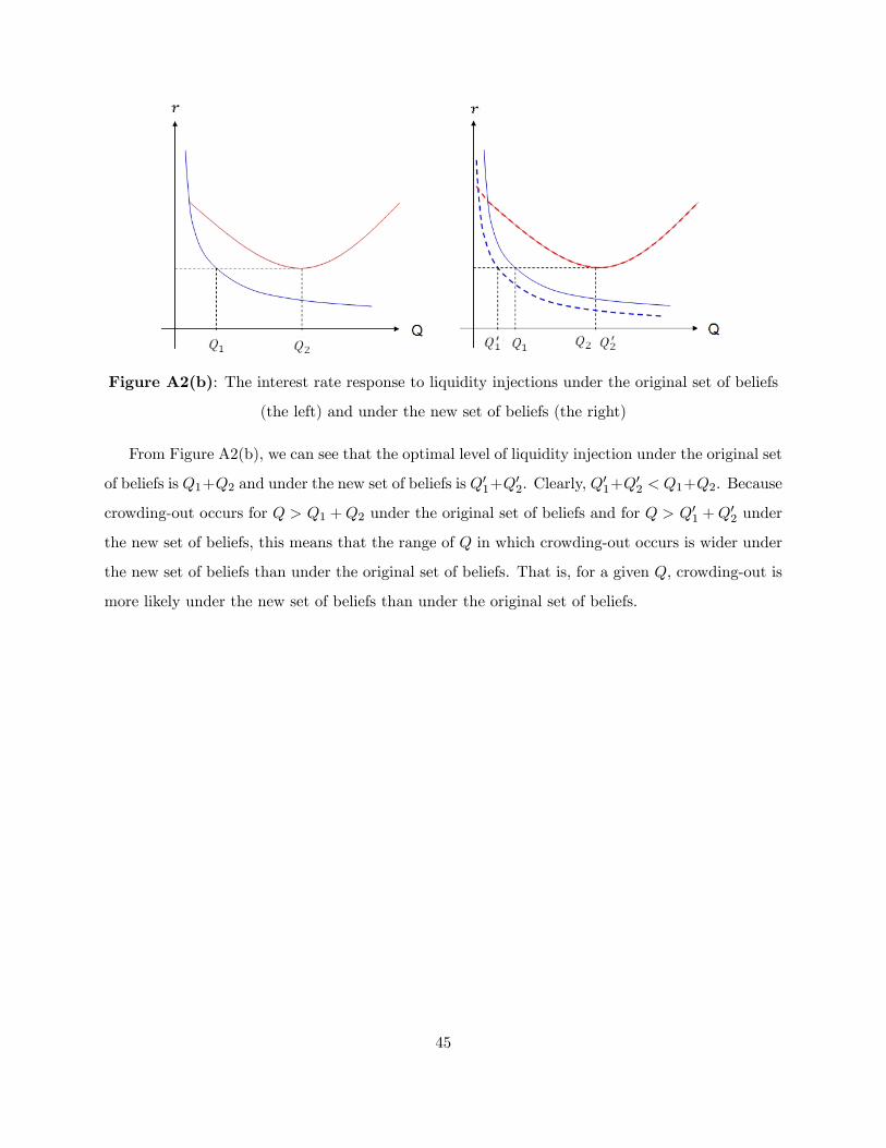
Figure A2(b): The interest rate response to liquidity injections under the original set of beliefs

(the left) and under the new set of beliefs (the right)

From Figure A2(b), we can see that the optimal level of liquidity injection under the original set

of beliefs is Q1+Q2 and under the new set of beliefs is Q01+Q02. Clearly, Q

01+Q

02 < Q1+Q2. Because

crowding-out occurs for Q > Q1 +Q2 under the original set of beliefs and for Q > Q01 +Q02 under

the new set of beliefs, this means that the range of Q in which crowding-out occurs is wider under

the new set of beliefs than under the original set of beliefs. That is, for a given Q, crowding-out is

more likely under the new set of beliefs than under the original set of beliefs.

45

Credit Expansion and Credit Misallocation

Documents

Transcript of Credit Expansion and Credit Misallocation