DI

SC

US

SI

ON

P

AP

ER

S

ER

IE

S

Forschungsinstitut zur Zukunft der ArbeitInstitute for the Study of Labor

Labor Supply and Consumption SmoothingWhen Income Shocks Are Non-Insurable

IZA DP No. 5499

February 2011

Alexander M. Danzer

Labor Supply and Consumption

Smoothing When Income Shocks Are Non-Insurable

Alexander M. Danzer Royal Holloway College, University of London, Ludwig-Maximilians-University Munich and IZA

Discussion Paper No. 5499 February 2011

IZA

P.O. Box 7240 53072 Bonn

Germany

Phone: +49-228-3894-0 Fax: +49-228-3894-180

E-mail: iza@iza.org

Any opinions expressed here are those of the author(s) and not those of IZA. Research published in this series may include views on policy, but the institute itself takes no institutional policy positions. The Institute for the Study of Labor (IZA) in Bonn is a local and virtual international research center and a place of communication between science, politics and business. IZA is an independent nonprofit organization supported by Deutsche Post Foundation. The center is associated with the University of Bonn and offers a stimulating research environment through its international network, workshops and conferences, data service, project support, research visits and doctoral program. IZA engages in (i) original and internationally competitive research in all fields of labor economics, (ii) development of policy concepts, and (iii) dissemination of research results and concepts to the interested public. IZA Discussion Papers often represent preliminary work and are circulated to encourage discussion. Citation of such a paper should account for its provisional character. A revised version may be available directly from the author.

IZA Discussion Paper No. 5499 February 2011

ABSTRACT

Labor Supply and Consumption Smoothing When Income Shocks Are Non-Insurable

The paper investigates how employees use secondary employment to smooth out consumption shortfalls from non-anticipated wage shocks in their main employment. The identification strategy exploits surprising changes in firms’ wage payment and repayment behavior in Ukraine. Based on unique nationally representative panel data, the econometric approach accounts for workers’ unobserved heterogeneity and measurement error in the wage shock information. The estimated labor supply responses suggest that secondary activities are used as temporary coping strategies against wage shocks and that they closely follow the lifecycle of wage arrears. Households that engage in secondary employment can successfully smooth their consumption. The results are robust to several alternative hypotheses concerning the observed labor supply pattern. JEL Classification: J22, J33, P36, O17 Keywords: dual job holding, wage shock, consumption smoothing, subsidiary farming,

reaction time to shocks Corresponding author: Alexander M. Danzer Department of Economics Ludwig-Maximilians-University Munich Geschwister-Scholl-Platz 1 80539 München Germany E-mail: alexander.danzer@lrz.uni-muenchen.de

1 Introduction How do workers respond to non-anticipated transitory wage shocks in their main

employment in a setting of imperfect markets, credit constraints and missing social security?

Particularly, do they re-allocate working time between the main job and additional jobs? The

goal of this research is to understand whether employees and their households are able to

smooth out consumption against negative wage shocks in the main job by adapting their

portfolio of activities. This is especially relevant if workers are unable to switch employers at

low costs, for instance because wage non-payment exerts a bonding effect towards the current

employer or because wage shocks are regionally concentrated.

The underlying theoretical framework of the paper is given by a simple dual job

holding model with random wage shocks in the main job, so that additional jobs can be taken

up in order to smooth out consumption shortfalls. The empirical analysis includes cross-

sectional and panel estimations based on a unique nationally representative data set from

Ukraine for the early 2000s. This case study setting is interesting as shortfalls in wage

payments were quite common (over 10% of the workforce each year) and as unusually rich

data on wage shocks are available. Coping activities were widely available so that employees

can either enter a second position as dependently employed worker or use smallholder

farming activities.

The paper addresses several potential empirical problems in the estimation of a

multiple job holding model. For instance, it deals with omitted variable bias by accounting for

unobserved heterogeneity through fixed effects estimation. The analysis also addresses

measurement error in the reported wage shocks by applying an instrumental variable (IV)

method that exploits the fact that firms’ pay practices were regionally highly concentrated.

The estimated labor supply responses to wage shocks indicate a re-allocation of

working hours from main to second jobs—with important differences between activities.

Exogenous variation in firms’ wage repayment is used to show the robustness of the identified

effects. As workers resemble participants of a lottery and cannot determine the arrival of wage

repayment, it is possible to test the motivation for holding second jobs and to study the

consumption smoothing behavior over the entire duration of the wage shock cycle. Further

support stems from the fact that none of the presented alternative hypotheses can

convincingly rival the consumption smoothing motive of second job holdings. This also

implies that there is no evidence for anticipatory behavior in the sense that workers might

respond to shocks ex-ante. In line with the estimated individual labor supply responses,

2

households cannot ex-ante insure their consumption against wage shocks but manage to

smooth out temporary shortfalls with the help of secondary activities.

The contributions of this paper are the following: This is the first empirical study to

analyze second jobs as a mode of consumption smoothing in the presence of main job wage

shocks. Combining three previously unrelated strands of literature on wage shocks, second

job holdings and consumption smoothing helps to gain new insights into how individuals and

households manage to cope with income shocks. Different from much of the previous

literature this paper exploits direct evidence on exogenous wage shocks. This unique variation

in wage levels allows to explicitly link firms’ wage policies to individual shock responses

over the entire duration of the earnings loss. Wage shocks have adverse effects on workers at

the time they occur, but this paper additionally analyzes the effect of the termination of the

shock—by using unique information on exogenous repayments. The analysis of both onset

and offset of wage shocks lends substantial robustness to the estimates. Finally, this study

extends the application of a dual job labor supply model to an emerging country context. The

research is based on the supposition that individuals are myopic and credit constrained which

seems quite realistic for many lower and middle income countries.

There are two main aspects of this research which are of particular policy relevance:

First, the analysis of wage shocks illustrates how firms’ payment policies affect labor supply.

Legal institutions that are too weak to enforce wage claims drive individuals into coping

mechanisms which might potentially imply an inefficient allocation of resources. This is

especially so when regional clustering of bad payment practices prevents regional labor

markets from functioning. Second, this paper investigates the question whether unanticipated

wage shocks can be smoothed out by individuals and households in imperfect capital markets,

i.e. when wage shocks cannot be insured. The impact of wage shocks is especially immediate

in a setting where household savings have been depleted and hence cannot be used to buffer

the shortfall and where the state does not provide any social security minimum.1 Low

mobility across jobs, sectors and regions prompts ‘on-the-job-responses’. Thus, the following

research addresses the ability of households to engage in self-help as well as the subsequent

welfare implications.2

1 Suffering from wage arrears does not entitle to the receipt of any state benefits. For the years prior to the Russian financial crisis 1998/1999, Guariglia and Kim (2003) found evidence for some precautionary saving behaviour in Russia. 2 As will be briefly discussed in the conclusion, the shift from main to second jobs may also change the role of the informal sector, which might be larger for second job holdings (cp. Guariglia and Kim, 2006).

3

The remainder of the paper is structured as follows: Section 2 reviews relevant

economic concepts of the labor allocation decision under uncertainty, multiple job holdings

and consumption smoothing. It also provides background information on the nature of wage

shocks and coping activities in Ukraine in the 2000s. Section 3 introduces the data sets.

Section 4 presents and discusses the econometric approach. The results concerning the

individual labor supply responses to wage shocks and the consumption smoothing abilities of

households are reported in Section 5. Section 6 discusses potential alternative hypotheses and

presents the results of several robustness checks. The final section concludes with policy

implications.

2 Background

2.1 Theoretical Background

One of the fundamental questions in labor economics is how individuals adapt their

labor supply in response to wage or income changes. Research on transitory wage shocks has

received limited attention for substantial time, as permanent income or consumption insurance

models pay disproportional attention to permanent shocks. Consequently, the modern inter-

temporal model of labor supply has largely ignored transitory wage shocks because it expects

them to play only an insignificant role in the life cycle labor supply decision.3 In recent years,

however, the interest in wage uncertainty and transitory wage shocks surged as the

assumptions of the inter-temporal labor supply model seem too restrictive. Mainly, the

suppositions of perfect foresight and the absence of credit constraints are inadequate for many

countries, and in particular in countries with incomplete markets and ongoing structural

change, like most developing and emerging countries. The latter setting prompts the use of the

myopic consumption model, in which individuals react to transitory shocks as they would

react to permanent ones (Jappelli and Pistaferri, 2006). Beside theoretical reasons in favor of

the study of transitory wage shocks, a higher econometric sensitivity to distinguish anticipated

from non-anticipated wage shocks has promoted research on unanticipated transitory wage

shocks—a field that had been ignored until recently (Pistaferri, 2003).

Three strands of literature are central to investigating the effect of wage shocks in the

main job on consumption smoothing through coping activities. In a standard labor supply

3 When the marginal utility of wealth is constant over time.

4

model with only one job, the effect of wage uncertainty on labor supply is theoretically

ambiguous. Block and Heineke showed that higher wage uncertainty leads to increased

working effort if the substitution effect towards leisure is dominated by the income effect in

the Hicks-Slutsky equation (Block and Heineke, 1973). However, this literature does not

allow for the possibility of second jobs. Around the same time, multiple job holding models

emerged with a particular focus on the labor supply behavior of individuals who face working

hours constraints in the main job. In their model of second job holdings, Shishko and Rostker

(1976) formally derived cross-wage labor responses and showed that individuals who are

hours constrained will increase second job labor supply with decreasing main job wage if

leisure is a normal good. An increase in non-labor income leads unambiguously to a decrease

in second job holdings through the income effect. Other authors describe alternative motives

to hold a second job—like the portfolio combination of stable and secure with casual

prestigious employment—without explicitly addressing the role of consumption smoothing

(Paxson and Sicherman, 1996; Smith Conway and Kimmel, 1998). The third strand of

literature focuses on consumption smoothing in general, and on the question how people

reduce income risk specifically. Different from the truly inter-temporal labor supply model

which expects transitory wage shocks to have no effect on labor supply, today’s perception is

that insurance is incomplete, especially for unexpected or low-frequency shocks. For both,

developing and developed countries, economists have presented evidence that shocks are not

perfectly insurable and that households engage in specific consumption smoothing activities

(Cochrane, 1991; Townsend, 1994; Attanasio and Székely, 2004).4 This paper combines all

three strands of literature in order to pay attention to the potential consumption smoothing

motive of secondary jobs, specifically against main job wage shocks. Myopic and credit-

constrained individuals cope with income shortfalls by reallocating effort between main and

second jobs. The novel aspect of this paper is that it focuses on within-person labor supply

responses which crucially depend on the availability of outside insurance options (Low,

Meghir and Pistaferri, 2010). In this respect this paper stands in contrast to the added worker

4 For countries with at least basic social security systems, one can expect that social protection indeed smoothes out labor market shocks—and simultaneously at least partly crowds out coping mechanisms (Cullen and Gruber, 2000). However, even under these conditions, increasing inequality over the life cycle is hard to explain when precluding the importance of uninsurable idiosyncratic risks (Storesletten, Telmer and Yaron, 2001).

5

literature, which investigates labor supply responses of married women to their husband’s

unemployment (Lundberg, 1985).5

The following analysis is based on a simple static model of labor supply. Individuals

are assumed to maximize utility U(c, l) which for simplicity only contains two arguments,

consumption c and leisure l. There are two main reasons for choosing a static model of labor

supply: First, Ukraine, the country under consideration, is a lower middle income country in

which individuals are severely credit constrained;6 thus a life cycle model which assumes

away credit constraints would be inappropriate. Second, the wage shocks which individuals

are facing in this setting (and which will be described in greater detail below) are

unanticipated so that employees can be assumed to behave myopically.

Employed individuals allocate effort h between two different jobs (subscript 1

indicating the main job and 2 indicating the optional secondary activities) subject to a total

time (T) constraint T = h1 + h2 + l with h1 > 0, h2 ≥ 0, the budget constraint y = w1h1 + w2h2

+ A, where w indicates the wage rate for main or second job and A is a measure of non-labor

income, as well as to a non-hiring constraint h1 + h2 ≤ T. In an environment of working hours

constraints, Sishko and Rostker (1976) have shown that a decrease in the main job wage rate

lets an individual shift effort towards the second job. It is straightforward to consider a similar

problem in a setup with a stochastic wage shock γ (as in Kurkalova and Jensen, 2000).

Kurkalova and Jensen show that the behavioral responses are ∂h2/γ >0 and ∂h1/γ <0.

2.2 Wage Arrears

Ukraine offers an interesting setting to analyze labor supply responses to wage shocks

under myopia and credit constraints: The high incidence of wage arrears in the country

provides an interesting source of exogenous variation in wage payments. But while wage

arrears were seen as a characteristic feature of post-Soviet labor markets in the mid-1990s,

they gained prominence in several countries during the recent global financial crisis (ILO,

2009). Even before, wage arrears had become increasingly problematic in some developing

and emerging countries, for instance, among migrant workers in China and the Middle East

(UNDP, 2005) and in many enterprises in India. In industrialized countries, wage arrears are

5 Consequently, one caveat of the analysis concerns the joint labor supply decision within households (Becker, 1965) which remains beyond the scope of this research. The labor force participation of women in Ukraine is quite high so that the scope for more spouses to enter the labor market is limited. 6 According to the World Bank (2008), access to financial intermediation in Ukraine even lags behind countries like Angola, Burkina Faso, Côte d’Ivoire, El Salvador, Libya and Mongolia—to name just a few.

6

of minor importance on the aggregate level and mostly appear temporarily when firms, e.g.

start-ups, undergo financially difficult times; however, more structural wage arrears can be

observed for the close-to-poverty part of the working population. In the UK, for instance,

wage arrears were problematic as a consequence of enterprises failing to pay at least the legal

minimum wage, especially before drastic fines and a short pay-back period were introduced in

2007.7

Arrears were initially understood as a consequence of decline in demand during the

recession or as a result of firms’ illiquidity.8 However, this perspective was challenged when

matched employer-employee data from Russia revealed that wage arrears were observable not

only in poorly-performing but also in many well-performing firms and that worker turnovers

remained relatively modest despite the substantial losses to individual incomes. From these

findings, Earle and Sabirianova (2002) developed an institutional theory of wage arrears

which understood wage non-payment as a function of managerial contract-violating behavior

and poor contract enforcing institutions.9 In other words, poor managerial behavior and

workers’ inability to enforce wage claims through courts led to substantial levels of wage

non-payment.10 Wage arrears were found to be sectorally and regionally highly correlated

with little structure across groups of workers so that the tacit collusion in contract violation

seriously restricted outside options for workers (Earle and Sabirianova, 2009).11 Hence, the

7 According to HMRC inquiries, 25,000 low-pay employees were affected by wage arrears in the UK in 2006 (BBC, 2007). 8 The neoclassical view of this phenomenon regarded wage arrears as a flexible tool to cushion the hardship of restructuring overstaffed state enterprises (Lehmann, Wadsworth and Acquisti, 1999; Desai and Idson, 2000). 9 The above cited study on China clearly depicts discrimination between home and migrant workers in China as main reason for wage arrears. Also in the UK, non-payment of legal minimum wages can be expected to reflect managerial behaviour rather than illiquidity of firms. 10 In most cases, workers did not file lawsuits, as courts were not assertive and their decisions had huge delays (cp. Earle, Spicer and Sabirianova, 2004). Court decisions in favor of workers were regularly ignored up until mid 2005, when a Ukrainian teacher won her case at the European Court of Human Rights (CFTUU, 2008). The Accounting Chamber of Ukraine states that “the systematic failings and infringements [...] identified [in wage non-payment] suggest an inadequate level of organization [...] and a lack of control” in many administrative bodies of Ukraine (UN CESCR, 2007: 14). 11 As a legacy from the Soviet Union, the existence of one-factory-towns and regionally concentrated economic sectors have clearly contributed to a geographic clustering of these shocks. Earle and Sabirianova (2002) argue that poor outside options in local labor markets might set free a self-enforcing spiral of wage arrears, as local entrepreneurs find it increasingly attractive to hold back wages. What is less well established is whether there was differential treatment of employees within firms and whether this might have induced worker selection. While Earle and Sabirianova (2002) find that leading positions in firms suffered less from wage arrears, Gerry, Kim and Li (2004) claim that firm managers allocated wage arrears according to equity principles, implying that the least earning workers were spared. To the opposite, Lehmann et al. (1999) find that regional and firm characteristics are strong predictors for wage arrears, while individual characteristics play a negligible role. All three papers use data from Russia and the only evidence on Ukraine from the 1990s reveals that personal characteristics play no significant role in the determination of wage arrears, while economic sector and regional location of the employee explain the incidence of arrears quite accurately (Boyarchuk, Maliar and Maliar, 2005).

7

local concentration of wage arrears diminished incentives to completely change employers.

This added to a generally low mobility of workers across jobs and sectors in transition

economies (Boeri and Flinn, 1999). When insurance and outside job options are missing,

leaving the region might be regarded as an alternative strategy in response to wage non-

payment. Yet, mobility rates in transition countries were generally low and even declining

despite a substantial rise in regional disparities (Fidrmuc, 2004).12 These specific features of

the regional labor markets make secondary activities a plausible alternative for risk

diversification.

In Ukraine, the incidence of wage arrears peaked at the end of the 1990s and declined

thereafter. Survey evidence for 1996 and 1999 shows that two third of employees suffered

from wage arrears in both years (Boyarchuk, Maliar and Maliar, 2005). According to the

International Labor Organisation, the average Ukrainian employee was owed the amount of

six monthly wage payments in the 1990s (ILO, 1996). Figure 1 illustrates that wage shocks in

the form of aggregate wage arrears were very high in the late 1990s. Starting at this extreme

incidence of wage non-payment, many Ukrainians were paid back outstanding wages during

the period of strong economic growth in the early 2000s. Still, the sum of wages owed by

current employers exceeded 1 percent of annual GDP in the years 2003 and 2004.13

Generally, there is no evidence of systematic sorting of workers across firms as a consequence of wage arrears (Earle and Sabirianova, 2002). 12 Reasons which may explain the low labor mobility and thus contribute to the persistence of shocks in certain regions include liquidity constraints, high search costs, administrative barriers and underdeveloped housing markets (Andrienko and Guriev, 2004). 13 As these aggregate figures exclude wage arrears from previous employers, they are likley to be underestimated.

8

Figure 1: GDP growth and aggregate level of wage arrears in Ukraine

-3%

0%

3%

6%

9%

12%

15%

0

500

1000

1500

2000

2500

3000

1997 1998 1999 2000 2001 2002 2003 2004 2005 2006 2007

Arrears (mln. USD; 1997 values), left scale

GDP growth (from previous year); right scale

Note: Unfortunately, no official statistics exist on wage arrears prior to 1997. Source: State Statistics Committee of Ukraine (http://www.ukrstat.gov.ua/), own calculations.

The repayment of arrears is one aspect that has been largely ignored in the literature.

Such paybacks did not only happen to employees who suffered from wage arrears with their

current employer but also to former employees who had left the firm in the past. Observations

from employer records and employee data indicate that repayments were “occasional and

lumpy” (Earle, Spicer and Sabirianova, 2004: 6). As no general bargaining process about the

repayment of wage arrears took place in Ukraine, the repayment decision has been taken by

the firm management on a monthly basis. So, depending on the predominant nature and cause

for wage arrears (liquidity constraints and/or managerial behavior), the repayment decision

might or might not be at the manager’s discretion.14 From the perspective of the individual

these repayments can be considered unanticipated. Some employees might not even work in

the indebted firm any longer and still receive a repayment. If negative wage shocks had a

causal and positive impact on secondary activities and if these activities were predominantly

used to fill the earnings gap, the repayment of wage shocks should have the opposite effect on

14 A simple test of the randomness of repayments is performed with the data set and variables described below: In a multivariate regression of the determinants of arrear repayments, none of the various demographic, job, firm and regional controls delivers a coefficient that is significantly different from zero at the 5 percent level. This indeed suggests that repayments had little structure.

9

labor supply. Thus, using repayment information as the analogue of wage shocks permits

shedding light on the true motivation for second job holdings.

2.3 Secondary Activities

Generally, work relations are still relatively inflexible in Ukraine. The main source of

rigidity is the strict Labor Code which has been in place since the Soviet era and which

regulates the working week to comprise 40 hours. Part-time arrangements are still the

exception. However, there are two sources of flexibility in the labor market: On the one hand,

there are increasing numbers of opportunities for employees to engage in second jobs in

dependent employment. Most second jobs comprise professional occupations (43%), followed

by manual (34%) and service occupations (23%). The sectors were most second job

employers operate are education, sales and maintenance, health, and other service activities

(56%), agriculture (19%), transport (8%), construction (6%) and are available throughout the

country; however, while only 1.6% of employees in villages hold a second job, the fraction is

typically much larger in towns and urban areas with up to 13.6% of employees in some cities.

On the other hand, many Ukrainians have opportunities for growing food on household plots

(subsidiary farming). Plot farming has a long tradition in Ukraine and other countries of the

former Soviet Union and is widespread in rural areas. In villages, more than 90% of

employees engage in at least some food production on a regular basis, while these numbers

are much lower in large cities—for instance only 10% of employees in the cities of Lviv and

Kiev. Farming requires access to plots and the availability of land naturally limits the

potential to use farming as a coping strategy. While these limitations are serious in cities,

availability of land is generally unproblematic in rural areas and small towns.15 Yet, starting

to produce food as a response to wage shortfalls is probably limited. Therefore we may expect

little response at the extensive margin for subsidiary farming (and if so only in areas where

access to land is good and prior engagement in farming imperfect, i.e. in small towns). More

easily, members of households that are already engaged in subsidiary farming could

potentially expand their activities (given that the survey was predominantly collected during

the agricultural season).

15 Due to a land sale moratorium, most plots are rented in.

10

3 Data and Descriptive Statistics Most of the following analysis rests on two waves from a relatively new panel data set,

the nationally representative Ukrainian Longitudinal Monitoring Survey (ULMS) for the

years 2003 and 2004. The ULMS is a rich data source combining individual level information

on socio-demographic characteristics with extensive labor-related data (Lehmann and Terrell,

2006).16 In addition, a household questionnaire collects rich information on household

composition, assets, income and consumption.17 After carefully cleaning the data and

restricting the sample to a balanced panel of prime age employees (17 to 60 years) who are

working throughout both waves, 1,736 individuals per year provide complete employment

and working hours information. Professional farmers, self-employed and family helpers are

excluded from the sample as wages and hence wage shocks are harder to define in their cases.

All individuals in the sample are employed and have worked for at least one hour in the

reference week and were paid or supposed to be paid a wage.18 This implies the exclusion of

employees on sick or maternity leave or in holidays. A variable overview for the sample can

be found in Table A1.

Additional data come from cross-sectional waves of the nationally representative

Ukrainian Household Budget Survey (UHBS) which collects information on 25,000

individuals and 9,000 households on an annual basis. The data comprise a rich set of

individual and household characteristics, information on employment as well as incomes. The

UHBS is here mainly used for estimating wage shock exposure and for imputing household

consumption. It provides information which is highly comparable to that of the ULMS but

includes more accurate indicators for outstanding wages from current and previous

employers.

16 The data were collected using multi-stage random sampling. If households moved between years, they were not followed across administrative regions (oblasts). 17 In 2003, information on household consumption was collected only rudimentary. Thus household consumption values for 2003 and 2004 are imputed from the extensive questionnaire on food, service and durables consumption in UHBS. This questionnaire is highly comparable to the one used in the ULMS household survey in 2004. To check the robustness of the imputations for 2004, consumption values from UHBS and ULMS for that year are compared indicating a very strong positive correlation (coefficient: 0.663; the R² in a simple regression is above 99 percent). 18 The overall share of employed persons in the survey rose from 45.7 percent to 47.3 percent between 2003 and 2004.

11

3.1 Wage Shock and Labor Supply Variables

Wage uncertainty is measured by worker-specific wage shocks which are defined as

wage payments that fall short of the contractual wage despite the fulfillment of contractual

work requirements. In other words, employees who report working normal hours in the

reference week (normal in comparison to their ‘work effort in an ordinary working week’) but

are paid no or a significantly lower wage than the contractually fixed amount and who report

that their employer owes them wage income, are classified as individuals suffering from wage

arrears. As also found for Russia (Earle and Sabirianova, 2002), wage arrears in the ULMS

data set exhibit a strong regional character. While some regions have a wage arrears incidence

of below 1 percent, up to 52 percent of employees were still affected in other areas in the

2003/2004 period. The variation across sectors is also substantial. While ‘only’ 4 percent of

employees in public administration suffered from wage arrears, more than every third

agricultural worker was affected (Table 1). Also, the conditional stock of back wages ranges

regionally from around one up to six months and was especially high in the transport,

agricultural and construction sectors.

Table 1: Wage arrears and secondary activities across sectors, 2003-2004

Share of workforce with

wage shock

Conditional number of

monthly wages in arrear

Second job holding

Subsidiary farming job

Agriculture 35.0% 3.7 2.0% 85.8% Industry 14.5% 2.1 2.1% 57.8% Electricity 12.8% 0.9 2.6% 64.4% Construction 5.6% 2.7 2.8% 50.0% Sale 4.7% 1.5 2.5% 48.9% Transport 6.2% 5.9 2.3% 65.5% Financial services 8.5% 2.2 4.3% 38.3% Public administration 4.1% 0.6 3.7% 63.0% Education 4.3% 0.8 2.7% 65.6% Other Services 8.4% 1.6 2.8% 50.2% Other 6.9% 2.0 0.0% 42.1% Note: 3,472 observations. Source: ULMS, own calculations.

As all individuals in the sample are employed in their main job, labor supply is

measured at the extensive margin by focusing on the participation decision in secondary

activities. Table 1 reveals that second job holdings are much less common than subsidiary

farming jobs, but both can be found across all economic sectors. At the intensive margin of

labor supply, working hours in the secondary activities are analyzed along with main job and 12

leisure hours. To impose as few assumptions as possible, leisure is defined as residual day

time. The computation subtracts from 24 hours: eight hours of sleep, the working hours in

main job, the working hours in other jobs and the time used for household food production.

Although consistency in the time use data was checked carefully and individuals who report

more than 99 hours of total work per week (including all sources of work) were excluded,

some individuals end up with slightly negative leisure per day. In general, the calculation

might still be correct, given that some individuals simply need less than eight hours for sleep

and personal care per day. Nevertheless, a strict minimum of 0.1 hours of leisure per day is

imposed in the analysis.

3.2 Control Variables

All regressions include as control variables individual characteristics (gender, age, age

squared/100, years of education, marital status) as well as regional (oblast) and settlement

type fixed effects and a common trend. To account for the time budget constraint and

exceptional work load during the reference period the natural logarithm of hours worked in

the main job is added as control. Further covariates include job characteristics (economic

sector of work, enterprise ownership19), different income measures (log of non-labor income,

the hourly wage rate and the second job shadow wage20) and a wealth (asset) indicator. Some

attention should be paid to the construction of the income, wage and welfare variables. As a

main job specific control variable, the hourly wage rate is constructed from contractual

monthly wage income divided by contractual monthly working hours. This variable thus

reflects how well a job would be paid under normal working and payment conditions. The

analysis accounts for non-labor income by using total consumption net of all members’ labor

incomes. To use household consumption rather than income helps to clean the analysis from

regular consumption smoothing activities (e.g. continuous household production of food from

small agricultural land plots) (cp. Blundell and MaCurdy, 1999). Furthermore, given that in

some households not all working age members provided income information (for reasons like

19 A variable indicating union membership status was not used in the regressions as it never came out significant. 20 The second job wage rate is obviously unobserved for those not holding a second job. Therefore a reduced form regression of the second job wage rate for second job holders is performed in order to predict a shadow wage for the entire sample. This procedure may later introduce selectivity bias as actual wages offered to those not holding a second job might be structurally lower than the ones offered to second job holders. As a consequence of this overprediction µ2 will be biased towards zero. Different from studies where individuals are predominantly hours constrained (Shishko and Rostker, 1976) the second job wage rate should play little role in this setting. All regressions have also been performed devoid of the second job shadow wage without any impact on the results.

13

absence at the interview date or refusal to participate in the survey), consumption seems the

more reliable measure. Household wealth is controlled for by a composite measure of ten

durable goods (e.g., refrigerator, washing machine, car etc.). Using principle component

analysis, the set of assets is transformed into an asset indicator which accounts for more than

57 percent of the overall variance in asset holdings. The correlation matrix of single assets

with the first principal component is reported in Table A2.

4 Methodology

4.1 The Labor Supply Equation

The main challenge of this research is to draw inference about the causal impact of

unanticipated wage shocks on labor supply. If wage shocks γ were purely random, one could

simply compare the change in second job holdings y (second job or subsidiary farming) over

time between those employees ‘treated’ with a wage shocks (γ=1) and those without a wage

shock (γ=0). Including as covariates the wage rates w1, w2 from the main and second job21

and household wealth A as well as individual characteristics X and firm and region controls J

gives the following formulation of the labor supply equation:

yit = α + β’Xit + δ1 γit + δ2 dt + µ1 w1it + µ2 w2it + µ3 Ait + σ’ Jit + εit 1

for i ∈ {1, ..., n}, t ∈ {2003, 2004}

The estimator of interest δ1 compares the conditional propensity of holding a second

job between individuals who experienced a wage shock with those without shock. As we

expect wage shocks to push workers into second jobs, δ1 should carry a positive sign. The

period dummy dt captures general time trends like nationwide changes to the demand for and

acceptability of second job holdings (e.g. employers in Ukraine might be increasingly ready

to employ workers on the basis of contracts with few hours per week). Initially, equation (1)

is estimated in a pooled OLS set-up with individual clustered standard errors. The hours

equation makes use of a normal rather than a log-log specification to implicitly account for

non-participation (Angrist and Krueger, 1999; Blundell and MaCurdy, 1999) and is estimated

with a censored Tobit model with clustered standard errors. Such a model assumes that the

21 No shadow wage has been imputed for subsidiary farming as producer food prices are unavailable.

14

participation decision and the hours decision are produced by the same econometric process

and that individuals who do not supply any labor to a second job simply chose zero hours. To

test the robustness of the estimated effects, two model specifications are used throughout all

main results. The first model employs only pre-determined demographic characteristics like

age, gender, education and pre-determined location controls. The second model is being

nested in the first and removes the parameter restrictions on all other covariates by adding all

remaining individual and job characteristics as well as measures for non-labor income and

asset wealth.22

All estimates might be biased if unobservable (and thus uncontrolled) factors

influenced both, the probability to suffer from a wage shock and the probability to take on a

second job. As a start, it is useful to think about the character of this bias and detect the

potential direction of its impact. One would expect that firm managers might impose wage

arrears on their less productive workers first, thus discriminating between workers of different

levels of ability or conscientiousness. The firm manager might be doing so, as she is able to

observe what remains unobservable to the researcher. In general, we expect that low levels of

ability or conscientiousness are negatively correlated with holding a second job, as second job

employers value similar characteristics as main job employers. Then, however, estimates

which cannot adequately account for unobservables should be downward rather than upward

biased.

Using panel data permits to control for unobservable individual characteristics. So, the

main econometric specification will account for individual heterogeneity by estimating (1) as

a fixed effects panel data model. In this way it is possible to remove any time-invariant

factors which potentially bias standard OLS. For the analysis of second job working hours,

the preferred model is the random-effects Tobit panel model.23

In order to take into account the possibility of measurement error in the shock

variable, a more comprehensive wage arrear measure from the larger UHBS data set is

exploited: it contains information on outstanding wages in the current job (as in the ULMS) as

well as from previous jobs. Similar to the ULMS, the UHBS asks respondents to indicate the 22 In order to test whether the more complex nested model has additional explanatory power, likelihood ratio (LR) tests are performed for the main tables. The reported p-values refer to the hypothesis that the simpler model is a valid representation for the nested model. In all cases, the LR test suggests the superiority of the more complex specification. 23 In addition a fixed-effects linear panel model is employed in order to show the robustness of the results for second job hours. This, however, estimates responses to wage shocks for the uncensored sample and will deliver coefficients that cannot be converted into effects for the sample under consideration (therefore these results are reported for illustrative purposes in Table A3 in the Appendix). It should be noted that censoring is strong for second jobs but not for subsidiary farming.

15

volume of outstanding wages while providing a much larger sample size. Hence wage shocks

can be measured quite accurately. The general model is again:

yit = β’Xit + δ1 γit + αi + εit       2

As this model is endangered to suffer from incorrectly measured wage shock

information γ, an instrument Z is employed. As the measurement problem cannot be solved in

the ULMS data set, auxiliary data (the UHBS) are used from which one can impute the wage

shock risk for the ULMS. The incidence of complete wage shocks (including arrears from

previous employers) is regressed on sector and region dummies in the UHBS data and then

predicted for ULMS observations as an instrument for wage uncertainty.24 In order to

estimate the parameter of interest (δ1) in the second stage, the first stage exploits the

conditional relationship between the observed wage shock variable and the assigned wage risk

information:

γit = β’Xit + λ Zit + uit       3  

This instrumental variable approach is estimated with generalized two-stage least

squares estimation (G2SLS) for panel data. As will be shown below, a Hausman test suggests

a preference for the more efficient random-effects panel model.

Albeit panel and IV methods correct different kinds of biases here, neither is as

conceptually straightforward as a quasi-experiment. One such experiment is represented by

the exogenous repayment of outstanding wages. Luckily, the availability of pay-back

information in Ukraine offers the unique opportunity to exploit exogenous variation in firms’

wage policies to understand the effect of wage shocks at the employee level over the entire

cycle of wage shocks.25

24 A matrix of 26 regions and 12 economic sectors is used in order to estimate wage shocks. To check the estimation fit in the prediction sample, a cross-validation of the prediction quality is performed by splitting the UHBS sample randomly and predicting the respective variable for the second part of the sample. The cross-validity coefficient of both sub samples is of reasonable size (+0.35). 25 In the UHBS data, 14 percent of repayments are directed to employees who have wage arrears with their current employer, while the substantial remaining share is received by those who have no arrears with the current but a former employer.

16

4.2 The Consumption Smoothing Equation

The final part of this paper addresses the question how successful credit constrained

households use secondary activities to smooth consumption. If the estimated effect of wage

shocks on labor supply was causal (i.e. employees ultimately respond to wage shocks) the

consumption smoothing mechanism of second job holdings should be traceable in the data.

Similar to the previous literature, this paper uses a household fixed effects consumption

model which can be consistently estimated even in a two-period set-up (Attanasio and

Székely, 2004):

Δlogcj = δ1Δlogyj + δ2Δsj + δ3Δlj + δ4Δ(lj*sj) + δ5Δ(fj*sj) + β’ΔXj + εj ; j є {1,..., n} 4

Under the absence of any consumption smoothing, the coefficient δ1 is expected to

converge to one, as consumption of household j perfectly covaries with available income. In

perfect insurance markets, the coefficient should not be different from zero, as consumption is

entirely independent of income. Furthermore, if insurance mechanisms were fully at work,

transitory shocks sj should have no impact on the level of consumption, thus the coefficient of

wage shocks δ2 should be zero. On the other hand, if the coefficient is statistically significant

different from zero and negative, transitory shocks seem not only to be unanticipated but also

ex-ante uninsurable. At the centre of interest here are the terms reflecting the response to

shocks (lj*sj) and (fj*sj) where lj is an indicator for second job holdings and fj for subsidiary

farming. The sign of δ4 and δ5 contains information on whether households that respond to

wage shocks by increasing their labor supply in a second activity can compensate for the

income loss and smooth out consumption. If δ2+δ3+δ4+δ5<0, households cannot entirely

shield their consumption against wage shocks. If δ2+δ3+δ4+δ5=0, households exactly

compensate for their income loss and if δ2+δ3+δ4+δ5>0, households are on average able to

overcompensate their loss. The fixed effects regressions also control for household size and

regional characteristics like access to finance26, which are subsumed under X.

26 Access to finance is measured as the regional share of households who either use a savings or lending facility at a bank. It should be noted, that households might potentially use savings to smooth out consumption. However, the Russian financial crisis of 1998/1999 depleted most of these savings.

17

5 Results The results of the empirical analysis are presented and discussed in the following

order: The first subsection provides a descriptive overview of the relationship between and

the determinants of the main variables of interest—wage shocks and secondary activities.

Then the causal effect of wage shocks on second job holdings is estimated, before the analysis

proceeds to the implementation of an IV approach in order to account for measurement error.

The final subsection turns to the role of wage shocks and coping mechanisms in the

consumption smoothing framework.

5.1 Descriptive Statistics

Those who currently suffer from a wage shock are more likely to engage in a

secondary activity. The top panel of Table 2 indicates that employees who experience wage

arrears have a 72 percent higher incidence of second jobs and a 12 percent higher incidence of

farming activities. Also working hours are significantly higher for employees with wage

shocks.

Wage arrears are not very persistent over time and across individuals. Panel B. of

Table 2 shows that entry to and exit from wage arrears status are substantial between the

years. Well above half of employees who suffered from a wage shock in 2003 do not report

any similar incidence in 2004, while 4 percent of employees without previous shocks

experience wage arrears in 2004. The substantial variation of wage arrears across individuals

over time is a crucial prerequisite for the outlined estimation strategy. It suggests that shocks

were not permanently concentrated among the same employees. Given the strong growth of

the economy in the early 2000s (see Figure 1) employees were probably not expecting wage

shocks in a way they might have been prepared for during the period of high shock incidence

in the 1990s. The crucial issue of employees’ anticipation will be more thoroughly addressed

in Section 6 of this paper.

Panel C. of the table shows the share of employees holding a second job in 2004 by

the same four cells of the wage arrears matrix. It becomes evident that those who have no

wage arrears in 2004 are less likely to engage in a second job, no matter whether they suffered

from insecure income in 2003. Their share of second job holders is around 2 percent.

Employees who suffer from wage shocks in both years are more likely to hold a second job

(2.7 percent). However, the highest second job holdings are recorded for those who have

wage shocks in 2004 but not in 2003. Six percent of them have a second job, suggesting that

the non-anticipated incidence of shocks might be the main driving force behind the observed

18

labor supply pattern. The pattern for subsidiary farming is quite different: Rather than current

shock incidence, last year’s experience seems to matter. This might be plausible given the

difficulties in land access and the inflexibility inherent to this coping strategy.27 Although

these unconditional results suggest that secondary activities and wage shocks are related, they

do not imply any causal relationship so far.

Before proceeding to the estimation of the shock response model it seems crucial to

gain a better understanding of the general determinants of second job holdings and wage

arrears. The determinants of wage shocks can shed light on whether arrears exhibit a pattern

of regional and sectoral concentration, as suggested by the previous literature on Russia.

Similarly, the determinants of secondary activities can suggest whether this kind of

employment is predominantly used by specific groups of employees.

Table 3 shows determinants of wage arrears in Ukraine based on a simple pooled

Probit model with individually clustered robust standard errors. Wage shocks are weakly

associated with gender and are more common among workers in their late 40s. The latter

finding is intuitive as the bonding effect exerted by arrears is stronger for older workers who

have already invested more in job and firm specific skills. Better off employees seem to have

a lower propensity to face wage arrears as indicated by the negative coefficient of the asset

variable. The main determinants of wage shock, however, seem to be region, sector and firm

effects with patterns that are in line with the previous literature (cp. Lehmann, et al., 1999).

The table also provides evidence on the determinants of secondary activities. Given

that overall only about 3 percent of employees hold a second job, the marginal effects are

small. Human capital and wealth are the main determinants of second job holdings, while

farming activities are correlated with region and sector characteristics. As expected, the

imputed second job shadow wage is positively correlated with second job holdings, but the

effect is almost negligible in size. An increase in the average second job hourly wage rate

from 10 UAH by 1 UAH (a plus of ten percent) would only imply an increase in the

propensity of holding a second job by 1.3 percent. Individual characteristics like gender, age

and marital status seem to play no significant role for second jobs but for subsidiary farming

activities where women and older workers are more likely to be engaged in.28 Two aspects

deserve special attention. First, employees who work fewer hours per week are more likely to

27 Having started a farming activity in the past might require further labor input beyond the termination date of the shock. Such prolonged coping seems quite realistic given that the average shock lasts around five months while the agricultural season might be longer. 28 An additional specification shows that married women are less likely to hold a second job.

19

perform a subsidiary activity. As will be shown later, this coefficient reflects a labor

substitution between main job and coping activity in the presence of wage shocks rather than

additional activities of workers who are involuntarily time constrained in the main job.

Second, non-labor household income and assets promote secondary activities. While both

coping strategies might be used against wage uncertainty in the main job, second jobs are

more common among the better-off and farming jobs are more widespread in rural areas.

Table 2: Incidence and intensity of secondary activities by wage shock status

Panel A. Participation in Second job holdings Subsidiary farming Currently no wage arrear 2.2% 60.7% Currently wage arrear 3.8% 68.6% Δ

1.6% (0.008)**

7.8% (0.027)***

Hours worked per week ina Second job Subsidiary farming Currently no wage arrear 4.5 15.2 Currently wage arrear 7.6 20.0 Δ

3.1 (1.10)***

4.8 (0.96)***

Panel B. Transition matrix No wage arrear 2004 Wage arrear 2004 Total No wage arrear 2003 96.0% 4.0% 100% Wage arrear 2003 56.9% 43.1% 100% Panel C. Second job holdings in 2004 No wage arrear 2004 Wage arrear 2004 Δ within row No wage arrear 2003 2.2% 6.0% 3.8%-p. (0.014)***Wage arrear 2003 2.4% 2.7% 0.3%-p. (0.015) Δ within column 0.3%-p. (0.010) -3.2%-p. (0.023)* Subsidiary farming in 2004 No wage arrear 2004 Wage arrear 2004 Δ within row No wage arrear 2003 60.3% 64.4% 4.1%-p. (0.046) Wage arrear 2003 70.6% 66.7% -3.9%-p. (0.045) Δ within column 10.2%-p. (0.032)*** 2.3%-p. (0.056) a conditional on participating in activity Note: Based on balanced panel of 3,472 observations. Source: ULMS, own calculations.

20

Table 3: Determinants of wage arrears and secondary activities

(1) (2)

(3)

Dependent variable Wage arrear Second job holding

Subsidiary farming

Probit Probit Probit Female -0.022* 0.003 0.044* (0.012) (0.004) (0.024) Age 0.010** 0.002 0.018** (0.004) (0.002) (0.008) Age squared/100 -0.011** -0.002 -0.015 (0.005) (0.002) (0.010) Adjusted years of schooling 0.004* 0.002** 0.003 (0.002) (0.001) (0.005) Centre 0.083** -0.006 0.323*** (0.043) (0.008) (0.038) West 0.039 0.017 0.316*** (0.039) (0.016) (0.036) East 0.133*** 0.002 0.326*** (0.046) (0.009) (0.039) South 0.048 0.012 0.252*** (0.038) (0.012) (0.044) Asset indicator -0.010*** 0.002 0.014* (0.004) (0.002) (0.008) Log of non-labor income 0.001 0.007*** -0.000 (0.003) (0.002) (0.006) Log of main job working hours -0.012** -0.086*** (0.005) (0.032) Second job shadow wage 0.0005*

(0.0003) 0.001

(0.001) Industry 0.052** 0.003 0.087** (0.027) (0.010) (0.038) Education -0.047** 0.000 0.085** (0.018) (0.010) (0.037) Agriculture 0.208*** 0.010 0.119** (0.052) (0.017) (0.045) De novo private firm -0.037** 0.008 -0.069* (0.012) (0.010) (0.036) Village -0.006 -0.003 0.454*** (0.014) (0.006) (0.018) Town -0.013 0.001 0.235*** (0.013) (0.005) (0.021) Time -0.034*** 0.002 -0.042*** (0.007) (0.003) (0.015) Pseudo R-squared 0.129 0.023 0.237 Observations 3472 3472 3472 Note: Marginal effects reported. Base categories are ‘Kiev region’, ‘large city’, ‘state enterprise’, ‘service sector’. All other coefficients on ‘married’, ‘privatized firm’, ‘national/international organization’, ‘Electricity’, ‘Construction’, ‘Sale’, ‘Transport’, ‘Administration’, and ‘Finance’ sector were insignificant. Robust standard errors clustered by individual ID are reported in parentheses. *** p<0.01, ** p<0.05, * p<0.1. Source: ULMS, own calculations.

21

5.2 Estimating the Effect of Wage Shocks on Secondary Activities

In the following we turn to the response of secondary activities to transitory wage

shocks. Table 4 reports results for different measures of wage arrears: a binary variable

indicating the presence of a shortfall of wages due to arrears (wage shock), the intensity of

wage shocks (measured as stock of outstanding monthly wages), an indicator for the receipt

of wage repayment29 and an indicator for the receipt of other positive wage shocks. The table

shows only the marginal effects of interest from regressions with several specifications. The

top panel comprises results for the naive pooled OLS estimation of equation (1), while the

bottom contains results from fixed effects regressions. Columns 1 and 3 control only for

exogenous demographic factors, while columns 2 and 4 add the remaining demographic, job

and welfare controls. The complete list of estimated coefficients of all regressors is provided

in Tables A4, A5a and A5b in the Appendix, which also contains the results based on

specification-specific maximal samples.

Second job holdings are 2.3 percentage points higher among employees with wage

shocks and these results are hardly affected by the inclusion of job and wealth controls. The

coefficient on shock intensity is positive, yet, insignificant. On the opposite, the repayment of

back wages significantly lowers the propensity to work in a second job and, interestingly, the

size of the coefficient is almost identical to the coefficient indicating the incidence of a wage

shock. Although these estimates are no more than correlations so far, this pattern might

suggest that the onset of a shock increase second job holdings, while the termination of the

shock reduces second jobs by the same rate. Such a co-movement of second job holdings with

wage arrears might be an indicator for a causal relationship. Finally, the analysis investigates

whether the repayment effect on second job holdings is simply driven by higher incomes. If

this was the case, higher than usual wage payments like bonus payments or gratuities should

have a similarly discouraging effect on second job holdings. However, positive wage shocks

other than wage repayments seem to be uncorrelated with second job holdings. Although all

estimates for subsidiary farming show the expected signs none of them is significant in this

specification.

If unobservable ability was negatively related to the propensity to suffer from a wage

shock but positively correlated to the propensity of holding a second job, the coefficients from

pooled OLS would be downward biased. As described earlier, the omitted variable (OV) is

29 Wage repayment means the explicit repayment of owed wages, not the return to scheduled monthly payment.

22

23

expected to be negatively correlated with wages shocks but positively correlated with second

job holdings. As the estimated coefficient on wage shocks in (1) is positive (Corr(OV, γ) < 0

and δ1 > 0), δ1 suffers from a negative bias. To account for this unobservable ability, fixed

effects are included in the estimation. The results reported in the lower panel of Table 4 show

that the causal impact of wage arrears on second job holdings becomes substantially larger

and remains statistically significant compared to OLS.30 Depending on the specification, the

coefficient is 13 to 22 percent larger when accounting for unobserved heterogeneity. As Table

4 further reveals, the intensity of wage shocks becomes now highly significant indicating that

each additional month of outstanding wages increases the probability of holding a second job

by 0.6 percent. The coefficient from the wage shock dummy specification is 4.7 times larger

than the coefficient in the intensity regressions, indicating that the average employee suffering

from a wage shock is owed 4.7 monthly wages. This number is indeed quite close to the

conditional sample mean for the shock intensity (see Table A1). The effect of wage

repayment becomes much larger in the fixed effects regression while other forms of positive

wage shocks remain insignificant, underlining that the estimated effects on second job

holdings cannot be simply attributed to additional income.

The incidence of wage shocks in the main job has a strong and positive significant

effect on subsidiary farming activities of employees residing in towns. The propensity to

engage in farming ranges between 13 and 16 percent. None of the intensity, repayment or

positive wage shock estimates turns out to be significant. While this might indicate that

individuals with access to land enter a continuous coping strategy, the lack of precision might

also stem from the limited size of the respective subsample.

30 The effect is significant in villages and towns as well as in large cities, where it is strongest (Table A7).

Table 4: Impact of wage shocks on secondary activities (extensive margin)

(1) (2) (3) (4) Dependent variable Second job holding Subsidiary farming job

Shock variable

Marg.eff. (std.er.)

R-Squared

LLa Marg.eff. (std.er.)

R-Squared

LLa (Prob > Chi2)

Marg.eff. (std.er.)

R-Squared

LLa Marg.eff. (std.er.)

R-Squared

LLa (Prob > Chi2)

OLS model Wage shock 0.023** 0.016 0.024** 0.020 0.009 0.103 0.017 0.126 (0.011) (0.011) (0.046) (0.047) Intensity of shock 0.004 0.018 0.004 0.022 0.003 0.103 0.003 0.126 (0.003) (0.003) (0.003) (0.003) Repayment -0.021** 0.013 -0.025*** 0.018 -0.359 0.104 -0.275 0.126 (0.009) (0.009) (0.349) (0.372) Positive shock 0.035 0.014 0.019 0.018 0.027 0.103 0.011 0.126 (0.034) (0.034) (0.137) (0.134) FE model Wage shock 0.028** 0.007 3616.0 0.027** 0.022 3643.0 0.158*** 0.088 121.2 0.128** 0.115 134.6 (0.013) (0.013) (0.000) (0.060) (0.064) (0.0315) Intensity of shock 0.006*** 0.013 3627.3 0.006*** 0.028 3652.9 0.003 0.073 114.4 0.004 0.107 130.6 (0.002) (0.002) (0.000) (0.006) (0.006) (0.0055) Repayment -0.202*** 0.008 3618.2 -0.195** 0.024 3645.2 -0.057 0.073 114.2 -0.111 0.107 130.4 (0.077) (0.077) (0.000) (0.306) (0.354) (0.0056) Positive shock -0.027 0.005 3612.8 -0.025 0.020 3639.4 0.055 0.073 114.3 0.102 0.108 130.9 (0.028) (0.028) (0.000) (0.132) (0.139) (0.0045) Demographic

controls X X X X

Job & welfare controls

— X — X

Observations 3472 3472 874 874 Note: Wage shock is defined as current wage arrear. Intensity is measured in number of monthly payments. Sample for (3) and (4) comprises only households residing in towns. All regressions control for individual demographics and regional controls. LR test for regressions (1) vs. (2) and (3) vs. (4): Prob > Chi2 (df 18). Robust standard errors in parentheses (clustered by id in OLS). a The LR test cannot be validly computed for clustered standard errors in the OLS model. *** p<0.01, ** p<0.05, * p<0.1. Source: ULMS, own calculations.

24

Beside the second job participation decision, wage shocks might prompt individuals to

intensify their activities in a previously existing second job. Table 5 presents the results from the

intensive labor supply margin in a Tobit and random-effects Tobit framework (for the full list of

regressors see Table A6). Individuals who already held a second job increase their labor supply

by around 5 hours following a wage shock (columns 1-4), a very consistent estimate across the

different specifications. This implies on average a doubling of second job hours after a wage

shock. Hours in subsidiary farming increase by 2.3 to 4.7 hours (columns 5-8). Interestingly, the

relationship between main job hours and hours in the secondary activity is comparatively small.

One additional hour in the main employment is associated with second job holdings that are on

average only one eighth of an hour lower. The effect is twice as large in subsidiary farming.

These results probably reflect the low variation in hours of main job employment relations,

where the vast majority of labor contracts are fixed at forty hours.

From a policy perspective, it is relevant to understand the mechanism which underlies

the increase in secondary activities or hours while employees are still employed in their main

job. The question is whether workers simply add more effort and increase their overall working

time at the expense of leisure or whether they re-allocate effort between jobs. On the one hand,

it seems reasonable to assume that employees reduced main job effort in exchange for second

job effort. On the other hand, the bonding effect of wage arrears might prevent them from

reducing effort significantly or from quitting the main job altogether (as a corner solution).

25

Table 5: Impact of wage shocks on working hours in secondary activities (intensive margin)

(1) (2) (3) (4)

(5) (6) (7) (8)

Dependent variable Working hours in second job Working hours in subsidiary farming Tobit Tobit RE

Tobit RE

Tobit Tobit Tobit RE

Tobit RE

Tobit Wage shock 4.761*** 4.631*** 4.729** 5.066*** 4.661*** 2.878** 3.932*** 2.293** (1.768) (1.779) (1.852) (1.917) (1.161) (1.215) (1.257) (1.112) Main job hours -0.100* -0.102* -0.129** -0.127** -0.200*** -0.231*** -0.212*** -0.240*** (0.058) (0.060) (0.062) (0.065) (0.035) (0.037) (0.045) (0.047) Log non-labor inc. 2.415*** 2.483*** -0.063 -0.043 (0.680) (0.690) (0.238) (0.246) Hourly wage main job 0.083 0.010 -0.632** -0.587 (0.370) (0.392) (0.299) (0.396) Demographic controls X X X X X X X X Job & wealth controls — X — X — X — X LL -574.82 -561.89 -550.19 -532.27 -6287 -6256 -6224 -6198 Prob > Chi2 (df 18) 0.0005 0.0074 0.0073 0.0120 Pseudo R2 / Chi2 0.034 0.056 27.2 33.7 0.0319 0.0367 312.1 1161 Observations 3472 3472 3472 3472 1834 1834 1834 1834 Note: Share of uncensored observations: 2.35%. The quadrature approximation of the RE Tobit model was checked using the ‘quadchk’ command in Stata. Sample for models (5) to (8) comprises only households in towns and villages. Robust standard errors in parentheses; *** p<0.01, ** p<0.05, * p<0.1. Source: ULMS, own calculations.

26

Furthermore, the hours constraint formulated earlier does not allow employees to provide

unlimited additional effort while being still employed in the risky main job. Table 6 therefore

also presents marginal fixed effects of main job hours and leisure with respect to wage shocks.

Suffering from a wage shock reduces main job hours supply by roughly 5 percent (columns 1-

3). Given that virtually all Ukrainians work 40 hours per week, the reduction of working time

equals 1.9 hours per week. This reduction is smaller than the associated increase in second job

labor supply implying that individuals must also reduce their available leisure time (columns 4-

6). On a weekly basis, the reduction ranges between 3.4 and 3.6 hours, depending on the

specification. Dividing the sample into three groups of individuals according to settlement type

shows that the reduction in main job and leisure hours takes place predominantly in villages and

towns where it amounts to minus 6.6 percent and minus 4.5 percent, respectively (Table A7).31

This is consistent with the availability of subsidiary farming opportunities in these areas.

So far we have seen that the incidence of wage shocks causes employees to engage in

secondary activities, while the subsequent repayment of outstanding wages significantly reduces

the likelihood of having a second job (but not of subsidiary farming). Table 7 adds another piece

of evidence to this cycle of entry and exit from second jobs by looking at the timing of the

events. While an adverse wage shock immediately reduces the disposable household income, the

search for a second job opportunity or the start of farming activities might be time-consuming.

Table 7 therefore reports current labor supply responses as a function of the timing of the shock.

As before, a current wage shock has a positive impact on second job holdings of around 2

percent and a marginally insignificant effect on subsidiary farming. A shock that took place

three to six months ago increases second job holdings and subsidiary farming twice as strong,

probably reflecting the individuals’ response time to the shock. Wage non-payments that arrived

for the first time nine to twelve months ago have no significant impact on current secondary

coping activities which appears reasonable given that wage shocks were relatively short lived

(on average 5.2 months). Again, this labor supply response pattern supports the idea that second

job holdings are co-moving with wage shocks.

31 While the top panel of Table 6 does not account for the main job hourly wage, the bottom panel also includes job characteristics. One of these characteristics is the log of the contractual hourly wage rate. As this variable is endogenous, the mean wage of employees of a specific educational level in a specific industry is used as an instrument. The IV estimation produces relatively large standard errors. The Marshallian wage elasticity of main job working hours is negative but not statistically significant different from zero. It suggests that employees do not adapt their working time in response to shifts in their earnings profiles. This seems reasonable as employees are severely constrained in their working time choices. It should be noted, that this elasticity does not make any statements about movements along the earnings profiles, given the static nature of the labor supply model.

27

28

Table 6: Responses in main job working hours and leisure

(1) (2) (3) (4) (5) (6) Dependent variables Log of main job hours Log of leisure hours FE FE FE FE FE FE

Wage shock -0.047* -0.055** Without job and wealth controls (0.026) (0.023) Shock intensity -0.002 -0.004 (0.003) (0.003) Repayment -0.123 0.026 (0.157) (0.137) Log of main job hours -0.433*** -0.431*** -0.431*** (0.021) (0.021) (0.021) LL 1135.04 1132.12 1132.45 1593.05 1589.57 1587.27 R-squared 0.006 0.004 0.004 0.198 0.197 0.196 Implied change in hours -1.9 -3.4 With job and wealth controls Wage shock -0.047* -0.057** (0.026) (0.023) Shock intensity -0.002 -0.003 (0.003) (0.003) Repayment -0.135 0.013 (0.157) (0.138) Log of main job hours -0.477*** -0.472*** -0.471*** (0.025) (0.025) (0.025) Log of hourly wage -0.026 -0.024 -0.023 -0.016*** -0.014*** -0.014*** (0.054) (0.054) (0.004) (0.005) (0.005) (0.005) LL 1145.67 1142.74 1143.22 1631.05 1625.99 1624.75 R-squared 0.012 0.010 0.010 0.216 0.214 0.213 Implied change in hours -1.9 -3.6 LR test, Prob > Chi2 (df 18) 0.000 0.000 0.000 0.000 0.000 0.000 Number of observations 3472 3472 3472 3472 3472 3472

Note: Mean leisure hours (week): 62.4; mean main job working hours (week): 40.9. Standard errors in parentheses; *** p<0.01, ** p<0.05, * p<0.1. Source: ULMS, own calculations.

Table 7: Response time to wage shocks

(1) (2) (3) (4) (5) (6)

Dependent variable Second job holding RE RE RE RE RE RE Current wage shock 0.023*** 0.024*** (0.009) (0.009) Shock 3-6 months ago 0.039*** 0.038*** (0.013) (0.014) Shock 9-12 months ago 0.026 0.023 (0.017) (0.017) Hausman test, chi2 12.25 14.41 14.75 20.42 22.05 22.33 df 10 10 10 26 26 26 Rho 0.351 0.349 0.350 0.350 0.348 0.349 Chi2 of model 39.63 40.93 34.62 67.32 68.24 61.98 R-squared 0.014 0.015 0.013 0.023 0.024 0.022 Observations 3472 3472 3472 3472 3472 3472 Dependent variable Subsidiary farming job RE RE RE RE RE RE Current wage shock 0.035† 0.033 (0.023) (0.025) Shock 3-6 months ago 0.063** 0.061** (0.030) (0.030) Shock 9-12 months ago 0.052 0.050 (0.037) (0.038) Hausman test, chi2 3.09 3.32 2.70 22.87 21.84 21.11 df 6 6 6 18 18 18 Rho 0.401 0.400 0.400 0.403 0.402 0.402 Chi2 of model 199.2 198.8 197.9 16748 16647 16563 R-squared 0.130 0.130 0.130 0.133 0.134 0.133 Observations 1834 1834 1834 1834 1834 1834 Demographic controls X X X X X X Job & wealth controls — — — X X X Note: Due to smaller sample size in the subsidiary farming model, some variables were removed from the model (place dummies, firm ownership). Critical value for df(6): 12.6, df(10): 18.3, df(18): 28.9 and for df(26): 38.9 at the 5% significance level. Robust standard errors clustered by id in parentheses. Hausman test is performed on unclustered data; *** p<0.01, ** p<0.05, * p<0.1, † p<0.15. Source: ULMS, own calculations.

29

5.3 Instrumental Variable Estimation

Previous results have shown that the incidence of a wage shock increases the

propensity to hold a secondary activity and the working hours therein. These results might be

confounded by measurement error in the right hand side variable thus attenuating the

estimated coefficient of interest. The relevant coefficient will then appear closer to zero than

the true estimate. To solve the potential bias from measurement error in the shock variable an

instrumental variable approach is applied. Table 8 and Table 9 show instrumental variable

estimates for both the extensive and intensive margin (the full first stage can be found in

Table A8). The participation equation and hour equation are both estimated with a random

effects G2SLS model. In all cases except one, the Hausman test indicates a preference for the

more efficient random effects model.

To condense information, the table provides only the estimates of interest. The RE

G2SLS model does not allow producing an F statistics to assess the strength of the instrument

directly; however, the z statistics for the instrumental variable in the first stage are very strong

for the second job participation and all hours equations (around 10-11) providing some

comfort regarding the predictive power of the instrument. Results for the second stage of the

2SLS suggest that wage shocks have a much bigger impact on the participation decision in a

second job than previously found in the OLS or FE models. The previously positive effect on

subsidiary farming, however, disappears in the IV approach. Unfortunately, analyzing the

effect of wage shocks in regional subsamples reduces the suitability of the instrument as it

builds on the regional variation of wage shocks. When estimated with G2SLS, the effect on

working hours becomes much smaller and suggests an increase in second job working time of

half an hour. However, it must be noted that in contrast to the Tobit model the G2SLS

estimation does not account for censoring in the hours equations. Coefficients can thus not be

directly compared. Table A3 reproduces a standard linear fixed-effects estimation of second

job working hours; its coefficients are the appropriate basis for comparison. The previous

estimates of 0.2 rose by around 170 to 190 percent when correcting the bias from

measurement error. In the subsidiary farming hours equation—which suffers only very little

from censoring—the estimates become more than twice as large after correcting for

measurement error. A wage shock thus induces an increase of almost 10 hours of working

time on the land plot. With the exception of the subsidiary farming participation equation all

instrumental variable estimates confirm the presence of measurement error so that previous

estimates in the participation and working time decisions were biased towards zero.

30

Table 8: G2SLS estimates of secondary activities

(1) (2) (3) (4)

(5) (6)

Dependent variable Second job holding

Subsidiary farming

RE RE RE RE RE RE Wage shock 0.127*** 0.123*** -0.028 -0.026 (0.046) (0.046) (0.146) (0.164) Wage shock intensity 0.032** 0.031** (0.015) (0.014) Log hours main job -0.012 -0.007 -0.029 (0.010) (0.013) (0.032) Log non-labor income 0.006*** 0.005*** -0.004 (0.002) (0.002) (0.005) Hourly wage main job 0.004* 0.003 -0.006 (0.002) (0.002) (0.010) Second job hourly wage 0.001*** 0.001** NA (0.000) (0.000) First stage (Dep. variable: wage shock) Wage shock risk (sector, region)

0.874*** (0.077)

0.868*** (0.076)

3.390*** (0.705)

3.402*** (0.702)

1.014*** (0.133)

0.907*** (0.131)

z-stats 11.16 11.38 4.81 4.85 7.60 6.90 Female -0.013 -0.042*** 0.007 -0.096 -0.018 -0.067*** (0.011) (0.011) (0.106) (0.107) (0.019) (0.020) Age 0.011*** 0.014*** -0.004 0.011 0.007 0.011* (0.004) (0.004) (0.036) (0.036) (0.007) (0.007) Age squared/100 -0.018*** -0.022*** -0.003 -0.020 -0.013 -0.018** (0.005) (0.005) (0.046) (0.046) (0.009) (0.009) Years of education 0.002 0.008*** 0.013 0.032 0.000 0.006 (0.002) (0.003) (0.022) (0.022) (0.004) (0.004)

-0.082*** -0.546*** -0.106*** Log of working hours main job (0.017) (0.141) (0.024) Demographic controls X X X X X X Wealth controls — X — X — X Hausman test, chi2 df

0.56 13

0.46 17

32.55 13

18.44 17

10.20 11

12.97 15

R-squared 0.010 0.013 0.011 0.012 0.146 0.147 Observations 3472 3472 3472 3472 1834 1834 Note: For full first stage results of (1) and (2) see Table A8. The regressions for the Hausman test were specified without time-invariant variables. The smallest critical value is for df(11): 19.7 at the 5% significance level. The critical value for df(13): 22.3 at the 5% significance level. Detailed region fixed effects and job characteristics are not controlled for, as they are measurement units for the shock instrument. Standard errors in parentheses; *** p<0.01, ** p<0.05, * p<0.1. Source: ULMS, own calculations.

31

Table 9: G2SLS estimates of hours in secondary activities

(1) (2) (3) (4) Dependent variable Hours in second job

Hours in subsidiary farming

RE RE RE RE Wage shock 0.551** 0.526** 9.942** 9.445** (0.268) (0.267) (4.156) (4.649) Log hours main job -0.081 -0.185*** (0.057 (0.035) Log non-labor income 0.028*** 0.085 (0.009) (0.224) Hourly wage main job -0.005 -0.487 (0.013) (0.367) Second job hourly shadow wage 0.002 (0.002) First stage (Dep. variable: wage shock) Wage shock risk (sector, region) 0.861*** 0.868*** 1.350*** 1.212*** (0.077) (0.076) (0.134) (0.133) z-value of instrument 11.16 11.38 10.11 9.14 Female -0.013 -0.042*** 0.007 -0.046** (0.011) (0.011) (0.019) (0.020) Age 0.011*** 0.014*** 0.012* 0.016** (0.004) (0.004) (0.007) (0.007) Age squared/100 -0.018*** -0.022*** -0.022** -0.025*** (0.005) (0.005) (0.009) (0.009) Years of education 0.002 0.008*** -0.002 0.005 (0.002) (0.003) (0.004) (0.005) Log of working hours main job -0.082*** -0.002** (0.017) (0.001) Demographic controls X X X X Wealth controls — X — X Hausman test, chi2 3.05 11.50 2.71 2.57 df 13 17 11 15 R-squared 0.010 0.013 0.106 0.129 Observations 3472 3472 1352 1352 Note: Models (1) and (2) treat censored values as uncensored. The sample of models (3) and (4) comprises only employees in towns and villages who were engaged in subsidiary farming in both years. For the full first stage results see Table A8. Due to smaller sample size in the subsidiary farming model, some variables were removed from the model (place dummies, firm ownership). The regressions for the Hausman test were specified without time-invariant variables. The smallest critical value is for df(11): 19.7 at the 5% significance level. Detailed region fixed effects and job characteristics are not controlled for, as they are measurement units for the shock instrument. Standard errors in parentheses; *** p<0.01, ** p<0.05, * p<0.1. Source: ULMS, own calculations.

32

5.4 Wage Shocks and Quitting Behavior

If workers were generally risk averse, they would always prefer to work in jobs with

lower wage uncertainty. Hence, after being affected by wage arrears once, they might be

inclined to change jobs. As noted by Earle and Sabirianova (2002) the nature of wage arrears

exerts a bonding effect, as leaving the firm might reduce the probability of being paid the full

amount of outstanding wages. The resulting trade-off between quitting and staying is an

empirical question. The availability of second jobs adds a twist to the quitting decision: When

faced with wage non-payment workers might prefer to search for second jobs first and quit

the main job as soon the second job can be turned into regular (full time) employment.

Unfortunately, the data do not permit the exact tracking of each specific employee-employer

relationship. Yet, this stepping stone hypothesis can be investigated by analyzing differences

in exit patterns of workers with and without wage shocks and workers who hold a second job

or not. The overall fraction of job changers between the 2003 and 2004 waves is 8.9 percent.

As the share of employees who switch job within one year is slightly higher among those who

currently suffer from wage arrears (10.1 percent), job quitting might dominate the bonding

effect; however, the difference is quite small.32 Table 10 estimates the conditional impact of

current wage arrears on the propensity to change job within one year. The coefficients on

both, wage shock indicator and wage intensity are positive—but only weakly significant.

Neither second job holdings themselves, nor the holding of a second job conditional on

suffering from a wage shock are significantly correlated to a job change in the future. This

implies that second jobs are not per se used as stepping stones towards new employment by

employees with risky job remuneration. Still, the coefficient on the interaction term between

shock intensity and second job holdings (column 4) is highly significant indicating that

workers with second jobs start leaving their main job as arrears accumulate.

32 It should be noted, that involuntary job separation rates are quite low in most transition countries (Brown and Earle, 2003). While Lehmann, Pignatti and Wadsworth (2006) find relatively high overall seperation rates for Ukraine, the share of involuntary layoffs is again modest. Also, self-employment is still very rare in Ukraine. The shares of entrepreneurial activities are higher in urban areas (2.8 percent) than in rural areas (2.4 percent), while more persons enter self-employment between 2003 and 2004 in rural areas (2.2 percent) than in urban areas (0.7 percent).

33

34

Table 10: Wage shocks and job change

(1) (2)

(3) (4)

Dependent variable Job change between t and t+1

Probit Probit Probit Probit Wage shock in t 0.034* 0.033* (0.022) (0.23) Intensity of wage shocks in t 0.003** 0.001 (0.001) (0.001) Second job holding 0.036 0.025 (0.047) (0.042) Wage shock/intensity*second job holding 0.099 0.025*** (0.144) (0.007) Demographic controls X X X X Job & wealth controls X X X X Pseudo R-squared 0.158 0.188 0.159 0.189 Observations 1736 1736 1736 1736

Note: Marginal fixed effects reported. The interaction term in column (2) is with wage shock, the one in column (4) with wage shock intensity. The estimation adopts a forward looking linear probability model. Robust standard errors in parentheses; *** p<0.01, ** p<0.05, * p<0.1. Source: ULMS, own calculations.

5.5 Consumption Smoothing

The smoothing model (equation 4) tests whether households whose members suffer

from a wage shock (at least one household member) consume less and whether they

successfully use secondary activities in order to smooth out these shortfalls (Table 11). The

coefficients on income indicate that consumption is co-moving with income, however, only

partially. The fact that the estimates are statistically different from zero but smaller than one

implies that consumption is positively related to current income but far from being perfectly

insurable against income fluctuations. Wage shocks within the household induce on average a

3 percent shortfall in household consumption, while second jobs per se do not significantly

affect consumption levels. As our outcome variable measures the log of total household

consumption, the fixed effect regressions also account for household size. Column (2) adds an

interaction term of wage arrear incidence with second job holdings. The coefficient thus

measures how consumption levels are affected in households that make use of second job

holdings in order to cope with wage shocks. The table shows a highly significant positive

coefficient; however, to study the effect of interest, the relevant measure is the joint

coefficient of δ2 + δ3 + δ4, which is reported at the bottom of the table. The hypothesis (H0)

under consideration is that households coping with second jobs cannot smooth out

consumption shortfalls from wage shocks, so δ2 + δ3 + δ4 < 0.

Table 11: Secondary activities as household consumption smoothing mechanisms

(1) (2) (3) (4) (5) (6) (7) (8) Full sample Full sample Rural sample Urban sample Full sample Rural sample Urban sample Full sample Dependent variable Log of household consumption FE FE FE FE FE FE FE FE Log of income 0.121*** 0.120*** 0.123*** 0.118*** 0.119*** 0.122*** 0.118*** 0.119*** (0.007) (0.007) (0.009) (0.010) (0.007) (0.009) (0.010) (0.007) Wage arrear in HH (δ2) -0.029** -0.040** -0.034 -0.045 -0.054** -0.053* -0.044 -0.059*** (0.012) (0.020) (0.024) (0.040) (0.022) (0.027) (0.040) (0.022) Second job in HH (δ3) -0.024 -0.045** -0.049 -0.033 -0.047** (0.021) (0.023) (0.033) (0.031) (0.023) Arrear*Second job (δ4) 0.099** 0.089 0.132* 0.102** (0.043) (0.056) (0.068) (0.043)

0.049** 0.055* 0.043 0.052** Arrear*Increase in sub-sidiary farming hours (δ5) (0.025) (0.031) (0.047) (0.025) Access to credit 0.418 1.516* -3.196 0.428 1.512* -3.209 0.445 (0.485) (0.817) (2.327) (0.485) (0.817) (2.330) (0.485) Arrear*Access credit 0.046 -0.098 0.075 0.078 -0.099 0.070 0.035 (0.234) (0.323) (0.384) (0.233) (0.318) (0.385) (0.234) Town 0.102** 0.158*** 0.106** 0.159*** 0.106** (0.044) (0.056) (0.044) (0.056) (0.044) Large city 0.134*** 0.139*** 0.139*** (0.046) (0.046) (0.046) Household size 0.082*** 0.082*** 0.083*** 0.075*** 0.082*** 0.083*** 0.075*** 0.082*** (0.006) (0.006) (0.008) (0.009) (0.006) (0.008) (0.009) (0.006) Constant 5.423*** 5.320*** 5.243*** 5.746*** 5.320*** 5.247*** 5.742*** 5.319*** (0.047) (0.063) (0.086) (0.189) (0.063) (0.086) (0.189) (0.063) (2)-(4): δ2 + δ3 + δ4 (5)-(7): δ2 + δ3 + δ5 (8): δ2 + δ3 + δ4 + δ5

0.014 (0.044)

0.044 (0.054)

-0.032 (0.076)

-0.005 (0.026)

0.001 (0.031)

-0.001 (0.055)

0.049 (0.047)

Hausman test, chi2 74.00 117.79 51.87 38.24 90.05 86.46 19.75 109.38 R-squared 0.219 0.224 0.235 0.212 0.223 0.235 0.209 0.226 Observations 4270 4270 2222 1886 4270 2222 1886 4270 Note: Highest critical value for models (2) and (8) with df(10): 18.3 at the 5% significance level. All Hausman tests rejected at the 1% level. Omitted category: Settlement village. Standard errors in parentheses; *** p<0.01, ** p<0.05, * p<0.1. Source: ULMS, own calculations.

35

Although δ2 + δ3 + δ4 are jointly positive, they are not statistically significant different

from zero. In other words, household suffering from a wage shock and using second jobs to

cope with them are no worse off than households without any wage shock. Column 2 also

accounts for access to the credit market which might be considered a tool for consumption

smoothing in developed economies. As expected in a setting of credit constraints, the

financial market plays no significant role in consumption determination and is not used as a

consumption smoothing tool. Columns 3 and 4 show results after splitting the sample into

rural and urban households. While second jobs seem to be a significant coping strategy for

urban households, they are marginally insignificant in rural areas. Overall, the joint coping

term is positive for rural areas and negative for urban areas, but the large standard errors leave

the effects insignificant. Rural households might use other coping strategies which buffer

their consumption levels against unforeseen shortfalls, like subsidiary farming. In columns 5

to 7, an interaction term between the incidence of current wage shocks and a dummy

indicating an increase of subsidiary farming hours is added to the model. This is done as the

previous analysis suggested more pronounced reactions at the intensive rather than extensive

margin of subsidiary farming. Indeed, rural households can significantly improve their

welfare situation by extending their farming activities, while this option seems less helpful fur

urban residents. The overall results suggest that farming is a successful coping strategy for

consumption smoothing in rural areas while second jobs are better suitable for urban areas.

Rural labor markets with their low dynamics seem incapable of absorbing transitory excess

labor supply. Column 8 includes both coping strategies at the same time into the consumption

smoothing model. All previous results remain robust.

In order to test the sensitivity of the results with respect to household size, Table A9 in

the Appendix replicates all results with adult equivalence scales. Such scales account for

economies of scales in household consumption. Oxford equivalence scales assign the

consumption weight of one to the first adult, 0.7 to all additional adults and 0.5 to all children

(aged up to 15) in the household. Applying this consumption correction does not change any

of the previous results.

6 Robustness and Alternative Hypotheses The following section evaluates potential alternative hypotheses which might explain

the observed labor supply patterns and hence pose a threat to the validity of the identified

results. In detail, the following section shows that the labor supply response in coping

36

activities cannot be explained by constrained working hours or by anticipatory ex-ante

coping.

6.1 Constrained Working Hours Hypothesis

One alternative explanation for the observed pattern of secondary activities refers to

the initial idea of second job holding models. The early literature analyzed second job

holdings in the USA, focusing mainly on constraints in working hours. These early model

applications were not associated with the consumption smoothing motive. Is it then possible

that second job holdings were merely driven by hours constraints? Some facts point into this

direction: Employees in Ukraine face a limited choice set of working hours. The Ukrainian

Labor Code stemming from the 1970s is restrictive with respect to contractual flexibility and

prescribes a weekly working time of 40 hours. Consequently, almost all employees are

contracted for exactly 40 hours. More flexible job contracts are starting to emerge slowly.

Only 4.4 percent of employees usually work less than full time.33 In our context, problems

would arise if enterprises that imposed wage arrears on their employees were at the same time

reducing labor demand. This might be plausible if wage arrears reflected negative demand

shocks to firms causing a simultaneous reduction of production and labor costs. In the

reference week, less than 1.6 percent of all employees report that they have worked fewer

than usual hours because they were either involuntarily sent home, because of work schedule

or because demand or input supply was too low. However, to check whether these groups of

workers might be more likely to take on a second job, the participation and hours regressions

are re-run with interactions of the wage arrear indicator and two dummies, one indicating that

a person is working fewer hours for demand reasons, the other one indicating involuntary

leaves from work (Table 12). Neither the variable indicating low demand nor the interaction

term has any impact on second job holdings. The compulsory leave dummy shows a positive

sign in the working hours model, suggesting that workers from firms that sent (part of) their

workforce home work on average two hours more in a second job. Less clear is the picture for

33 Additional 9.8 percent of employees report less than 40 hours work per week, but claim to be considered full-time workers as their contractual work load is lower than 40 hours. This applies in specific, often hazardous, occupations, for night work and for employees aged up to 18 years. The latter group, however, is excluded from the sample. As a robustness check, regressions for part-time and full-time subsamples are run separately. Part-time employment is defined as having worked at most 35 hours per week in 2003. The results are qualitatively the same, with part-time workers being slightly more likely to hold a second job (albeit with imprecise point estimate owing to the small part-time sample). Part- and full-time workers show a similar response to wage arrears (Table A10). This is not surprising, given that main job working hours are controlled for in the standard analysis.

37

38

subsidiary farming: While low labor demand plays no role for the amount of hours supplied

on land plots, general participation in farming is higher among employees in firms with low

demand but no wage shocks.34 To further investigate the hypothesis of constrained working

hours, contractual and actual hours of work are compared instead of self-reported absence

from work. When interacting the wage shock indicator with a dummy variable that takes on

the value of one if an employee simultaneously works less than contractual and suffers from a

wage arrear (and zero otherwise) the previous results are robust. A final check uses

information on desired working hours among those who were reporting less than forty hours

in the reference week.35 If under normal circumstances time constraints limited these

employees, one would expect them to respond with a desired labor supply of more than forty

hours. However, 91 percent of those working less than forty hours in the reference week

would like to work up to forty hours only. Among those suffering from wage arrears, the

share of those wanting to work more than 40 hours is even lower (6.7 percent) and this group

is no more likely to hold a second job. Reduced working time alone cannot explain the switch

towards second job holdings. This leads to the conclusion that wage shocks have a negative

impact on main job hours through the shift towards second job holdings, not vice versa.

Employees thus substitute away effort from the risky main job towards the second job.

6.2 Anticipation of Wage Shocks

If wage shocks are more likely to appear in some firms or sectors than in others,

workers might observe these differences and sort into sectors or firms according to their risk

aversion. However, workers employed in at-risk jobs or occupations should be aware of the

risk they face and, hence, ex-ante respond to their potential wage shortfalls with precautionary

behavior (cp. Low et al., 2010). In that case, the measured labor supply effect might reflect

the anticipatory behavior of at-risk workers rather than ex-post coping strategies. To test the

anticipation hypothesis a model is estimated whether workers who will suffer from shocks in

period t+1 already adapt their labor supply in period t. The coefficients of the forward looking

regressions are shown in Table 13.

34 There are too few observations for involuntary leaves in towns, so that columns (3) and (6) are not replicated for subsidiary farming jobs. 35 The question on desired working hours is only asked to individuals who work fewer than 40 hours in the reference week.

Table 12: Response to wage shocks in firms with low labor demand or involuntary leaves

(1) (2) (3) (4) (5) (6)

(7) (8) (9) (10)

Dependent variables Second job holding Hrs. in second job Subsidiary farming Hrs. in subsid. farming FE FE FE RE Tobit RE Tobit RE Tobit FE FE RE Tobit RE Tobit Wage shock 0.028** 0.026** 0.029** 4.758*** 2.639** 3.910*** 0.128** 0.154** 2.391** 2.340* (0.013) (0.013) (0.013) (1.788) (1.195) (1.432) (0.064) (0.063) (1.048) (1.248) Low labor demand -0.005 -1.456 0.371** 4.933 (0.028) (3.681) (0.155) (5.336)

0.108 6.971 -0.494* -0.695 Wage shock*Low labor demand (0.066) (5.593) (0.255) (10.602) Involuntary leave -0.017 1.884* (0.172) (1.015)

0.010 -5.094 Wage shock*Involuntary leave (0.199) (180.9) Demographic controls X X X X X X X X X X Job & wealth controls X X X X X X X X X X Rho 0.530 0.523 0.529 0.683 0.271 0.110 0.631 0.620 0.387 0.384 LL 3630.9 3630.5 3627.8 -547.9 -598.6 -587.7 134.6 131.8 -6209 -6208 R-squared / Chi 2 0.015 0.015 0.016 24.33 32.63 33.76 0.115 0.110 1615 1298 Observations 3472 3472 3472 3472 3472 3472 874 874 1834 1834 Note: The sample for subsidiary farming comprises individuals residing in towns, while sample for hours in subsidiary farming comprise individuals residing in towns or villages. Involuntary leaves were quite rare, so that the estimation of model (3) and (6) was not repeated for subsidiary farming. Standard errors in parentheses; *** p<0.01, ** p<0.05, * p<0.1. Source: ULMS, own calculations.

39

None of the anticipation coefficients on future wage shocks carries a significant

positive sign, implying that precautionary behavior is absent. Column 6 shows a

negative anticipation effect on subsidiary farming hours; this counter-intuitive result is

only significant at the 10 percent level and might reflect a type I error. These general

results are in line with the presumption that the incidence of wage shocks has a random

component. Consequently, non-anticipation of shocks supports the choice of a

framework with myopically behaving agents.

A related explanation for the detected shock response pattern could be associated

with past shock experience. The more distant experience of wage shocks is picked up by

the individual fixed effects as a ‘common history’. Furthermore, having suffered from

wage shocks during the 1990s should not have any impact on today’s precautionary

behavior as wage shocks then were virtually omnipresent in Ukraine. More recent wage

shocks could, however, make the difference: In order to test this hypothesis, a variable

indicating the incidence of a wage shock 9 to 12 months ago is included in the models

alongside the current wage shock dummy. If recent past wage shocks promoted

precautionary second job holdings, this variable should pick up part of the estimated

coping effect from the current shock. As can be seen from Table 14, the estimates of

labor supply responses to wage shocks are almost identical to previous results after

controlling for previous shock experience. At the same time, the coefficient of past

shock experience is insignificant. This finding further underlines the fact that second

jobs are used as immediate coping mechanisms in response to wage shocks.

In sum, the pattern of secondary activities cannot be explained by the rivaling

hypotheses about hours constraints and precautionary coping behavior. In an online

appendix to this paper, further robustness tests provide evidence that the estimated

effects are not confounded by panel sample attrition (Tables A11a, A11b, A12a, A12b).

40

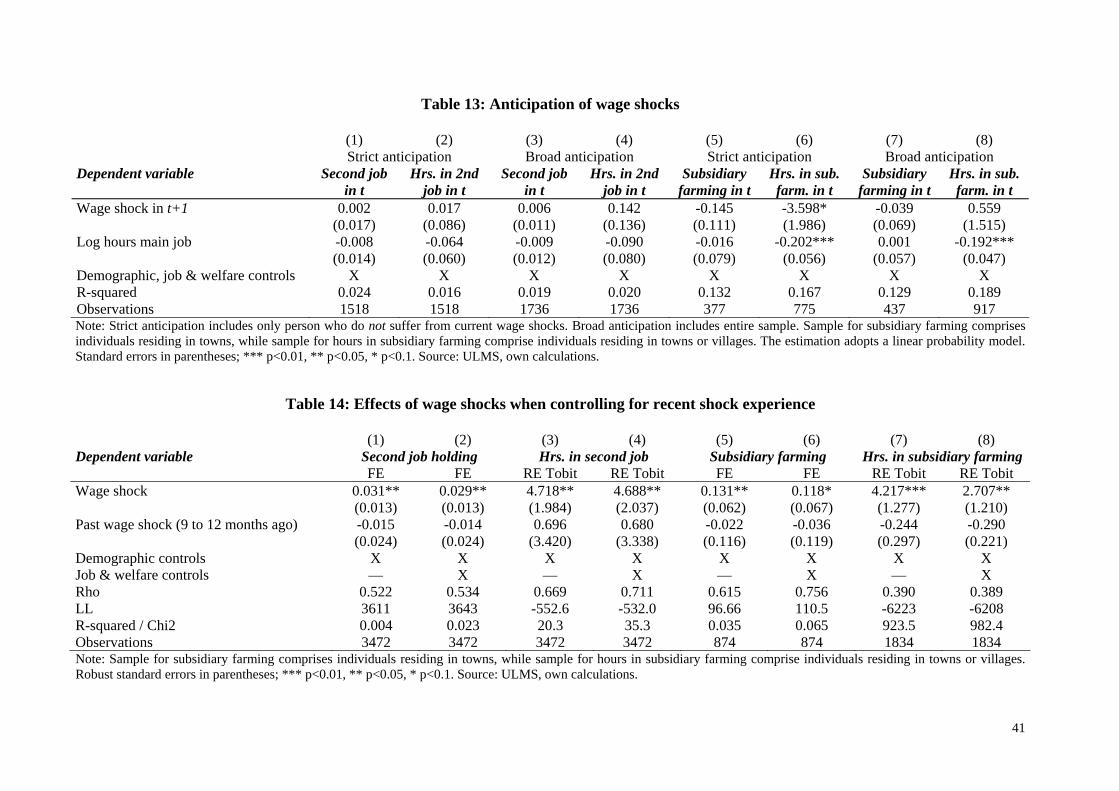
Table 13: Anticipation of wage shocks

(1) (2) (3) (4) (5) (6) (7) (8) Strict anticipation Broad anticipation Strict anticipation Broad anticipation Dependent variable Second job

in t Hrs. in 2nd

job in t Second job

in t Hrs. in 2nd

job in t Subsidiary

farming in t Hrs. in sub. farm. in t

Subsidiary farming in t

Hrs. in sub. farm. in t

Wage shock in t+1 0.002 0.017 0.006 0.142 -0.145 -3.598* -0.039 0.559 (0.017) (0.086) (0.011) (0.136) (0.111) (1.986) (0.069) (1.515) Log hours main job -0.008 -0.064 -0.009 -0.090 -0.016 -0.202*** 0.001 -0.192*** (0.014) (0.060) (0.012) (0.080) (0.079) (0.056) (0.057) (0.047) Demographic, job & welfare controls X X X X X X X X R-squared 0.024 0.016 0.019 0.020 0.132 0.167 0.129 0.189 Observations 1518 1518 1736 1736 377 775 437 917 Note: Strict anticipation includes only person who do not suffer from current wage shocks. Broad anticipation includes entire sample. Sample for subsidiary farming comprises individuals residing in towns, while sample for hours in subsidiary farming comprise individuals residing in towns or villages. The estimation adopts a linear probability model. Standard errors in parentheses; *** p<0.01, ** p<0.05, * p<0.1. Source: ULMS, own calculations.

Table 14: Effects of wage shocks when controlling for recent shock experience

(1) (2) (3) (4) (5) (6) (7) (8) Dependent variable Second job holding Hrs. in second job Subsidiary farming Hrs. in subsidiary farming FE FE RE Tobit RE Tobit FE FE RE Tobit RE Tobit Wage shock 0.031** 0.029** 4.718** 4.688** 0.131** 0.118* 4.217*** 2.707** (0.013) (0.013) (1.984) (2.037) (0.062) (0.067) (1.277) (1.210)

-0.015 -0.014 0.696 0.680 -0.022 -0.036 -0.244 -0.290 Past wage shock (9 to 12 months ago) (0.024) (0.024) (3.420) (3.338) (0.116) (0.119) (0.297) (0.221)

Demographic controls X X X X X X X X Job & welfare controls — X — X — X — X Rho 0.522 0.534 0.669 0.711 0.615 0.756 0.390 0.389 LL 3611 3643 -552.6 -532.0 96.66 110.5 -6223 -6208 R-squared / Chi2 0.004 0.023 20.3 35.3 0.035 0.065 923.5 982.4 Observations 3472 3472 3472 3472 874 874 1834 1834 Note: Sample for subsidiary farming comprises individuals residing in towns, while sample for hours in subsidiary farming comprise individuals residing in towns or villages. Robust standard errors in parentheses; *** p<0.01, ** p<0.05, * p<0.1. Source: ULMS, own calculations.

41

7 Conclusions This paper tested whether individuals use secondary activities as consumption

smoothing devices against transitory wage shocks, in a setting of myopic and credit

constrained agents. The empirical analysis is based on a unique panel data set from Ukraine

which provides detailed information on employment relations, wages and wage non-payment.

The results suggest a significantly positive albeit small effect of the incidence of wage shocks

and shock intensity on second job holdings and a sizeable effect on subsidiary farming in

areas with access to land plots. Working hours are increased in second jobs and subsidiary

farming by 3 to 5 hours while main job hours and leisure time are reduced in a similar order

of magnitude. Exogenous repayment of outstanding wages is used as a supportive quasi-

experiment to test the coherence of the temporary coping hypothesis. The data reject several

alternative explanations for the observed activity choices, like hours constraints in the main

job and the anticipation of shocks.

These findings prove robust when accounting for unobserved heterogeneity of

employees by controlling for fixed effects. Most estimates become quantitatively larger after

correcting potential measurement error in the shock variable with an instrumental variable

approach.

To test the effectiveness of the coping behavior a simple econometric test of

household consumption smoothing is carried out. It reveals that non-anticipated transitory

wage shocks cannot be perfectly insured ex-ante. However, households whose members cope

with wage shocks by re-allocating work effort from main to secondary job manage to keep up

their consumption levels. Hence, secondary activities enable households to fully smooth out

income shortfalls from wage arrears. The results are in line with the general consumption

smoothing literature which suggests that individuals and households put coping mechanisms

in place when insurance and foresight are imperfect. The presented evidence is thus consistent

with the prediction from the static theory of labor supply.

The findings from this research have several interesting policy implications. First, in

the absence of protective social security institutions individuals strive to engage in secondary

activities as coping mechanisms in order to reduce the consequences of wage shocks. This

evidence indicates that individuals and households might manage to feed themselves;

however, politics that rely on this mechanism must keep in mind how limited the scope for

self-help might be, e.g. through low demand on the second job market or weather risks.

42

Second, the paper has shown how firms’ wage payments may lead to diversification on the

labor market and thus spill-over from firm policies on labor supply. The results suggest that

employees do not entirely retreat from the labor market but on average reduce main

employment effort in substitution for secondary activities. Potentially these jobs may be less

productive or informal implying negative consequences for tax revenues. Third, the

reallocation of work may impact on the regional labor supply, as wage shocks were found to

be regionally highly concentrated. The previous research on wage arrears in transition

countries has regarded the clustering of wage risks in combination with low job mobility as

the main reason why employees refrain from switching employers after shocks. This paper

delivers another aspect which has been ignored in the literature so far: If coping mechanisms

for consumption smoothing were widely available in the short run, workers might feel less

pressure to switch jobs.

Acknowledgment

I thank Joshua Angrist, Deborah Cobb-Clark, Peter Dolton, Dan Hamermesh, Victor

Lavy, Hartmut Lehmann, Jonathan Wadsworth and Natalia Weisshaar as well as seminar and

conference participants at Royal Holloway, Amsterdam (EALE), Mannheim (ZEW), Milan

(EEA) and Berlin (ESCIRRU) for helpful comments and suggestions The ULMS data were

kindly provided by the ESCIRRU consortium and DIW Berlin. The usual disclaimer applies.

43

References

Andrienko, Yuri, and Sergei Guriev. 2004. “Determinants of interregional mobility

in Russia.” Economics of Transition 12: 1–27.

Angrist, Joshua D., and Alan B. Krueger. 1999. “Empirical Strategies in Labor

Economics.” In Handbook of Labor Economics, ed. Orley Ashenfelter, and David Card,

1463-1555.

Attanasio, Orazio, and Miguel Székely. 2004. “Wage shocks and consumption

variability in Mexico during the 1990s.” Journal of Development Economics 73(1): 1-25.

BBC. 2007. http://news.bbc.co.uk/1/hi/uk/6243307.stm

Becker, Gary S. 1965. “A Theory of the Allocation of Time.” Economic Journal

75(229): 493-517.

Block, Michael K. and John M. Heineke. 1973. “The Allocation of Effort Under

Uncertainty: The Case of Risk Averse Behavior.” Journal of Political Economy 81(2): 376-

85.

Blundell, Richard, and Thomas MaCurdy. 1999. “Labor Supply: A Review of

Alternative Approaches.” in Handbook of Labor Economics Volume 3A, ed. Orley C.

Ashenfelter and David Card, Ch. 27. Amsterdam: Elsevier Science Publishers BV.

Boeri, Tito, and Christopher J. Flinn. 1999. “Returns to Mobility in the Transition

to a Market Economy.” Journal of Comparative Economics 27(1): 4-32.

Boyarchuk, Dmytro, Lilia Maliar, and Serguei Maliar. 2005. “The consumption

and welfare implications of wage arrears in transition economies.” Journal of Comparative

Economics 33(3): 540-564.

Brown, J. David, and John S. Earle. 2003. “The Reallocation of Workers and Jobs

in Russian Industry: New Evidence on Measures and Determinants.” Economics of Transition

11(2): 221–252.

CFTUU (= Confederation of Free Trade Unions of Ukraine). 2008. “International

News Bulletin.” Newsletter 2, Vol. 1, 2.

Cochrane, John H. 1991. “A Simple Test of Consumption Insurance.” Journal of

Political Economy 99(5): 957-976.

Cullen, Julie B., and Jonathan Gruber. 2000. “Does unemployment insurance

crowd out spousal labor supply?” Journal of Labor Economics 18(3): 546-558

44

Desai, Padma, and Todd Idson. 2000. Work without Wages. Russia’s Nonpayment

Crisis. Cambridge, MA: MIT Press.

Earle, John S., and Klara Z. Sabirianova. 2002. “How late to pay? Understanding

wage arrears in Russia.” Journal of Labor Economics 20(3): 661-707.

Earle, John S., and Klara Z. Sabirianova. 2009. “Complementarity and Custom in

Wage Contract Violation.” Review of Economics and Statistics 91(4): 832-849.

Earle, John S., Andrew Spicer, and Klara Z. Sabirianova. 2004. “Community

Norms and Organizational Practices: The Legitimization of Wage Arrears in Russia, 1992-

1999.” IZA Discussion Paper, IZA Bonn, No. 1006.

Fidrmuc, Jan. 2004. “Migration and regional adjustment to asymmetric shocks in

transition economies.” Journal of Comparative Economics 32(2): 230-247.

Gerry, Christopher J., Byung-Yeon Kim, and Carmen A. Li. 2004. “The Gender

Wage Gap and Wage Arrears in Russia: Evidence from the RLMS.“ Journal of Population

Economics 17(2): 267-288.

Guariglia, Alessandra, and Byung-Yeon Kim. 2003. “Wage arrears uncertainty and

precautionary saving in Russia.” Economics of Transition 11(3): 493-512.

Guariglia, Alessandra, and Byung-Yeon Kim. 2006. “The dynamics of

moonlighting in Russia. What is happening in the Russian informal economy?” Economics of

Transition 14(1): 1-45.

ILO. 1996. “Growing Discontent on Wage Arrears in CIS.” ILO SRO-Budapest

Bulletin, 2/96. URL: http://www.ilo.org/public/english/region/eurpro/ budapest/info/bul/96-

2/nl10_11.htm [accessed 10 March 2010]

ILO. 2009. “Global Wage Report.” URL: http://www.ilo.org/wcmsp5/groups/public/--

-dgreports/---dcomm/documents/publication/wcms_116500.pdf [accessed 15 September

2010].

Jappelli, Tullio, and Luigi Pistaferri. 2006. “Intertemporal Choice and Consumption

Mobility.” Journal of the European Economic Association 4(1): 75-115.

Kurkalova, Lyubov A., and Helen H. Jensen. 2000. “Relative Growth of Subsidiary

Farming in Post-Soviet Economies: A Labor Supply Story.” Center for Agricultural and Rural

Development, Iowa State University, WP 249.

Lehmann, Hartmut, Norberto Pignatti, and Jonathan Wadsworth. 2006. “The

incidence and cost of job loss in the Ukrainian labor market.” Journal of Comparative

Economics 34(2): 248-271.

45

Lehmann, Hartmut, and Katherine Terrell. 2006. “The Ukrainian Labor Market in

Transition: Evidence from a New Panel Data Set.” Journal of Comparative Economics, 34(2):

195-199.

Lehmann, Hartmut, Jonathan Wadsworth, and Alessandro Acquisti. 1999.

“Crime and Punishment: Job Insecurity and Wage Arrears in the Russian Federation.”

Journal of Comparative Economics 27(4): 595-617.

Low, Hamish, Costas Meghir, and Luigi Pistaferri. 2010. “Wage risk and

employment risk over the life cycle.” American Economic Review 100(4): 1432-1467.

Lundberg, Shelly. 1985: “The Added Worker Effect.” Journal of Labor Economics

3(1): 11–37.

Paxson, Christina H., and Nachum Sicherman. 1996. “The dynamics of dual job

holding and job mobility.” Journal of Labor Economics 14(3): 357-393.

Pistaferri, Luigi. 2003. “Anticipated and Unanticipated Wage Changes, Wage Risk,

and Intertemporal Labor Supply.” Journal of Labor Economics 21(3): 729-754.

Shishko, Robert, and Bernard Rostker. 1976. “The Economics of Multiple Job

Holdings.” American Economic Review 66(3): 298-308.

Smith Conway, Karen, and Jean Kimmel. 1998. “Male labor supply estimates and

the decision to moonlight.” Labor Economics 5: 135-166.

Storesletten, Kjetil, Chris I. Telmer, and Amir Yaron. 2001. “How important are

idiosyncratic shocks? Evidence from labor supply.” American Economic Review 91(2): 413-

417.

Townsend, Robert M. 1994. “Risk and Insurance in Village India.” Econometrica

62(3): 539-591.

UN CESCR. 2007. “Parallel Report to the UN Committee on Economic, Social, and

Cultural Rights by the Ukrainian Helsinki Human Rights Union and the International

Renaissance Foundation regarding Ukraine’s implementation of the International Covenant

on Economic, Social and Cultural Rights.” Helsinki.

UNDP. 2005. China Human Development Report 2005—Human Development with

Equity. Beijing.

Wooldridge, Jeffrey M. 2002. Econometric Analysis of Cross Section and Panel

Data. Cambridge, MA: The MIT Press.

World Bank. 2008. Finance for All. Washington D.C.

46

Online Appendix – Not intended for publication

47

48

Appendix A: Tables

Table A1: Overview of variables

Variable Mean Min Max Labor market information Second job 2.3% 0 1 Hours second job h2 0.12 0 24 Conditional hours in second job, (h2 | h2 > 0) 5.1 0.5 24 Subsidiary farming 61.5% 0 1 Hours subsidiary farming h2 9.5 0 98 Conditional hours in subsidiary farming, (h2 | h2 > 0) 14.6 0 98 Hours in main job (reference week) 40.9 1 100 Leisure time (hours per week) 62.3 12 109 Wage shock Prob(γ > 0) (arrear) 10.6% 0 1 Intensity of shock γ (number of arrear months) 0.30 0 69 Conditional intensity of shock γ, (γ | γ > 0) 5.2 0.1 69 Repayment 0.14 0 1 Effort related positive shock 1.2% 0 1 Demographic characteristics Female 54.9% 0 1 Married 71.9% 0 1 Age 40.6 17 60 Adjusted years of schooling 12.0 4 15 Regional characteristics Village 27.4% 0 1 Town 27.4% 0 1 City 45.2% 0 1 Kiev (region) 5.5% 0 1 West (region) 18.7% 0 1 East (region) 27.2% 0 1 South (region) 24.9% 0 1 Centre (region) 23.7% 0 1 Welfare indicators Asset indicator 0.3 -3.398 4.346 Log of non-labor income 5.5 0 9.1 Job characteristics Contractual hourly wage in main job 2.2 0.1 45 Economic sector 1 12 Business ownership category 1 4 Note: Sample size: 3,472 (balanced sample). Source: ULMS, own calculations.

Table A2: Correlation matrix for asset items and asset indicator

Color TV PC Phone Mobile phone

Refriger-ator

Washing machine Car Motorcycle Dacha

Other apartment, house

Color TV 1 PC 0.1338 1 0.000 Phone 0.2362 0.1877 1 0.000 0.000Mobile phone 0.1636 0.2821 0.1462 1 0.000 0.000 0.000Refrigerator 0.3892 0.1004 0.2316 0.1287 1 0.000 0.000 0.000 0.000Washing machine 0.3108 0.1237 0.2022 0.1389 0.3281 1 0.000 0.000 0.000 0.000 0.000Car 0.1828 0.1398 0.191 0.2116 0.1596 0.1949 1 0.000 0.000 0.000 0.000 0.000 0.000Motorcycle 0.0625 -0.0387 -0.0298 -0.0139 0.0344 0.0573 0.0248 1 0.000 0.000 0.000 0.082 0.000 0.000 0.002Dacha 0.0907 0.0755 0.1399 0.0639 0.0891 0.0881 0.1111 0.0114 1 0.000 0.000 0.000 0.000 0.000 0.000 0.000 0.154Other apartment, house 0.0177 0.0273 0.0132 0.0608 0.0084 0.0282 0.0291 0.0349 0.0769 1 0.027 0.001 0.097 0.000 0.290 0.000 0.000 0.000 0.000Score for component 1 0.6491 0.4401 0.5609 0.4777 0.6254 0.6078 0.5038 0.0592 0.2966 0.0996 0.000 0.000 0.000 0.000 0.000 0.000 0.000 0.000 0.000 0.000

Note: Reported values are factor predictions from Principal Component analysis. Sample size: 3,472 (balanced sample). The table displays pair wise correlation coefficients; p-values of significance levels in italics. Source: ULMS, own calculations.

49

Table A3: Hours responses to wage shocks, intensive margin

(1) (2) (3) (4) (5) (6)

Dependent variable Hours in second job FE FE FE FE FE FE Wage shock 0.206** 0.182* (0.093) (0.094) Intensity of wage shock 0.082*** 0.080*** (0.011) (0.011) Repayment -1.505*** -1.474*** (0.553) (0.557) Log hours main job -0.169** -0.170** -0.182** -0.222** -0.231** -0.245** (0.085) (0.084) (0.085) (0.100) (0.098) (0.100) Demographic controls X X X X X X Job & wealth controls — — — X X X R-squared 0.007 0.034 0.008 0.017 0.043 0.019 Observations 3472 3472 3472 3472 3472 3472 Note: Regressions for illustration only. Robust standard errors in parentheses; *** p<0.01, ** p<0.05, * p<0.1. Source: ULMS, own calculations.

50

Table A4: Full list of main regressors, extensive margin, OLS model

Comparison of maximal sample (col. 1 to 8) with constant sample size (col. 9 and 10)

(1) (2) (3) (4) (5) (6) (7) (8) (9) (10)

Dependent variable Second job holding indicator (0/1) Maximal sample Maximal sample Constant sample OLS OLS OLS OLS OLS OLS OLS OLS OLS OLS Wage arrear 0.021** 0.023** 0.023** 0.024** (0.010) (0.010) (0.011) (0.011) Number of arrears 0.004 0.004 (0.003) (0.003) Repayment -0.026*** -0.028*** (0.008) (0.009) Positive shock 0.032 0.031 (0.033) (0.035) Female 0.001 0.001 0.000 0.000 0.002 0.002 0.001 0.000 0.003 0.002 (0.005) (0.005) (0.005) (0.005) (0.006) (0.006) (0.006) (0.006) (0.006) (0.006) Age 0.002 0.002 0.002 0.002 0.003 0.003 0.003 0.003 0.001 0.003 (0.002) (0.002) (0.002) (0.002) (0.002) (0.002) (0.002) (0.002) (0.002) (0.002) Age squared/100 -0.003 -0.003 -0.003 -0.003 -0.004 -0.004 -0.004 -0.004 -0.002 -0.004 (0.002) (0.002) (0.002) (0.002) (0.003) (0.003) (0.003) (0.003) (0.003) (0.003) Years of education 0.004*** 0.004*** 0.004*** 0.004*** 0.004*** 0.004*** 0.004*** 0.004*** 0.004*** 0.003** (0.001) (0.001) (0.001) (0.001) (0.001) (0.001) (0.001) (0.001) (0.001) (0.001)

0.001* 0.001* 0.001 0.001 0.001 0.001 0.001 0.001 0.001* 0.001 Second job hourly shadow wage (0.000) (0.000) (0.000) (0.000) (0.000) (0.000) (0.000) (0.000) (0.000) (0.000) Log hours main job -0.027*** -0.026** -0.027*** -0.027*** -0.021* -0.021* -0.023* -0.024** -0.021* -0.020 (0.010) (0.010) (0.010) (0.010) (0.012) (0.012) (0.012) (0.012) (0.011) (0.013) Village -0.001 -0.001 -0.000 0.000 -0.001 -0.001 -0.000 -0.000 -0.008 -0.005 (0.007) (0.007) (0.007) (0.007) (0.007) (0.007) (0.007) (0.007) (0.008) (0.008) Town -0.004 -0.004 -0.004 -0.004 0.000 -0.000 -0.000 -0.000 -0.002 -0.000

51

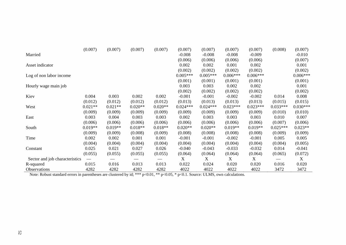
(0.007) (0.007) (0.007) (0.007) (0.007) (0.007) (0.007) (0.007) (0.008) (0.007) Married -0.008 -0.008 -0.008 -0.009 -0.010 (0.006) (0.006) (0.006) (0.006) (0.007) Asset indicator 0.002 0.002 0.001 0.002 0.001 (0.002) (0.002) (0.002) (0.002) (0.002)

0.005*** 0.005*** 0.006*** 0.006*** 0.006*** Log of non labor income (0.001) (0.001) (0.001) (0.001) (0.001)

Hourly wage main job 0.003 0.003 0.002 0.002 0.001 (0.002) (0.002) (0.002) (0.002) (0.002) Kiev 0.004 0.003 0.002 0.002 -0.001 -0.001 -0.002 -0.002 0.014 0.008 (0.012) (0.012) (0.012) (0.012) (0.013) (0.013) (0.013) (0.013) (0.015) (0.015) West 0.021** 0.021** 0.020** 0.020** 0.024*** 0.024*** 0.023*** 0.023*** 0.033*** 0.030*** (0.009) (0.009) (0.009) (0.009) (0.009) (0.009) (0.009) (0.009) (0.010) (0.010) East 0.003 0.004 0.003 0.003 0.002 0.003 0.003 0.003 0.010 0.007 (0.006) (0.006) (0.006) (0.006) (0.006) (0.006) (0.006) (0.006) (0.007) (0.006) South 0.019** 0.019** 0.018** 0.018** 0.020** 0.020** 0.019** 0.019** 0.025*** 0.023** (0.009) (0.009) (0.008) (0.009) (0.008) (0.008) (0.008) (0.008) (0.009) (0.009) Time 0.002 0.002 0.001 0.001 -0.001 -0.001 -0.002 -0.001 0.005 0.005 (0.004) (0.004) (0.004) (0.004) (0.004) (0.004) (0.004) (0.004) (0.004) (0.005) Constant 0.025 0.021 0.027 0.026 -0.040 -0.043 -0.033 -0.032 0.014 -0.041 (0.055) (0.055) (0.055) (0.055) (0.064) (0.064) (0.064) (0.064) (0.065) (0.072) Sector and job characteristics — — — — X X X X — X

R-squared 0.015 0.016 0.013 0.013 0.022 0.024 0.020 0.020 0.016 0.020 Observations 4282 4282 4282 4282 4022 4022 4022 4022 3472 3472

Note: Robust standard errors in parentheses are clustered by id; *** p<0.01, ** p<0.05, * p<0.1. Source: ULMS, own calculations.

52

Table A5a: Full list of main regressors, extensive margin second job holdings, FE model Comparison of maximal sample (col. 1 to 8) with constant sample size (col. 9 and 10)

(1) (2) (3) (4) (5) (6) (7) (8) (9) (10)

Dependent variable Second job holding indicator (0/1) Maximal sample Maximal sample Constant sample FE FE FE FE FE FE FE FE FE FE Wage arrear 0.027** 0.027** 0.028** 0.027** (0.011) (0.013) (0.013) (0.013) Number of arrears 0.006*** 0.006*** (0.001) (0.002) Repayment -0.170** -0.195** (0.068) (0.077) Positive shock -0.023 -0.025 (0.026) (0.028) Age -0.006 -0.007 -0.005 -0.006 -0.012 -0.015 -0.011 -0.013 -0.012 -0.012 (0.014) (0.014) (0.014) (0.014) (0.023) (0.023) (0.022) (0.022) (0.023) (0.023) Age squared/100 0.008 0.010 0.007 0.008 0.011 0.014 0.010 0.012 0.013 0.011 (0.016) (0.016) (0.016) (0.016) (0.020) (0.020) (0.020) (0.020) (0.020) (0.020) Years of education -0.003 -0.003 -0.003 -0.003 -0.002 -0.002 -0.002 -0.002 -0.002 -0.002 (0.003) (0.003) (0.003) (0.003) (0.003) (0.003) (0.003) (0.003) (0.003) (0.003)

0.001 0.001 0.001 0.001 -0.000 0.000 0.000 0.000 0.001 -0.000 Second job hourly shadow wage (0.004) (0.004) (0.004) (0.004) (0.005) (0.005) (0.005) (0.005) (0.005) (0.005) Log hours main job -0.022** -0.023** -0.024** -0.024** -0.020 -0.022 -0.023* -0.023 -0.026** -0.020 (0.011) (0.011) (0.011) (0.011) (0.014) (0.014) (0.014) (0.014) (0.012) (0.014) Town -0.011 -0.013 -0.013 -0.013 -0.010 -0.012 -0.011 -0.011 -0.012 -0.010 (0.018) (0.018) (0.018) (0.018) (0.020) (0.019) (0.021) (0.021) (0.019) (0.020) Time 0.007 0.007 0.006 0.006 0.008 0.009 0.008 0.008 0.007 0.008 (0.009) (0.009) (0.009) (0.009) (0.014) (0.014) (0.013) (0.013) (0.014) (0.014) Married 0.026* 0.027* 0.027* 0.027* 0.026*

53

(0.015) (0.015) (0.015) (0.015) (0.015) Asset indicator -0.003 -0.003 -0.003 -0.003 -0.003 (0.004) (0.004) (0.004) (0.004) (0.004) Log of non labor income 0.005** 0.005** 0.005** 0.005** 0.005** (0.002) (0.002) (0.002) (0.002) (0.002) Hourly wage rate main job 0.002 0.001 0.001 0.001 0.002 (0.003) (0.002) (0.002) (0.003) (0.003) Constant 0.228 0.260 0.237 0.246 0.295 0.385 0.334 0.335 0.390 0.332 (0.329) (0.328) (0.329) (0.330) (0.641) (0.640) (0.639) (0.640) (0.639) (0.665) Sector and job characteristics — — — — X X X X — X R-squared 0.007 0.012 0.007 0.005 0.022 0.028 0.024 0.020 0.007 0.023 Observations 4282 4282 4282 4282 4022 4022 4022 4022 3472 3472 Note: Robust standard errors in parentheses are clustered by id; *** p<0.01, ** p<0.05, * p<0.1. Source: ULMS, own calculations.

Table A5b: Full list of main regressors, extensive margin, subsidiary farming, FE model Comparison of maximal sample (col. 1 to 8) with constant sample size (col. 9 and 10)

(1) (2) (3) (4) (5) (6) (7) (8) (9) (10)

Dependent variable Subsidiary farming indicator (0/1) Maximal sample Maximal sample Constant sample FE FE FE FE FE FE FE FE FE FE Wage arrear 0.131** 0.106* 0.158*** 0.128** (0.057) (0.063) (0.060) (0.064) Number of arrears 0.003 0.003 (0.006) (0.006) Repayment -0.070 -0.253 (0.314) (0.338) Positive shock 0.037 0.071 (0.135) (0.138)

54

55

Age -0.036 -0.043 -0.039 -0.040 0.026 0.020 0.028 0.025 0.038 0.022 (0.103) (0.104) (0.104) (0.104) (0.113) (0.113) (0.113) (0.113) (0.112) (0.115) Age squared/100 0.042 0.048 0.044 0.045 -0.025 -0.020 -0.028 -0.025 -0.040 -0.022 (0.097) (0.097) (0.097) (0.097) (0.104) (0.104) (0.104) (0.104) (0.103) (0.106) Years of education 0.010 0.009 0.010 0.010 0.009 0.008 0.009 0.009 0.002 0.002 (0.013) (0.013) (0.013) (0.013) (0.013) (0.013) (0.013) (0.013) (0.013) (0.014) Log hours main job -0.008 -0.018 -0.018 -0.018 -0.005 -0.021 -0.019 -0.021 0.023 0.006 (0.050) (0.050) (0.050) (0.050) (0.059) (0.058) (0.058) (0.058) (0.053) (0.060) Time -0.156 -0.142 -0.142 -0.142 -0.053 -0.039 -0.041 -0.039 -0.074 -0.060 (0.100) (0.100) (0.100) (0.100) (0.113) (0.113) (0.113) (0.113) (0.109) (0.113) Married -0.001 0.005 0.003 0.004 -0.006 (0.079) (0.080) (0.079) (0.079) (0.081) Asset indicator -0.019 -0.017 -0.017 -0.017 -0.017 (0.017) (0.017) (0.017) (0.017) (0.017) Log of non labor income 0.000 -0.000 0.000 0.000 -0.001 (0.012) (0.012) (0.012) (0.012) (0.012) Hourly wage rate main job -0.021 -0.027* -0.026* -0.027* -0.020 (0.014) (0.014) (0.014) (0.014) (0.014) Interview month: June 0.123 0.103 0.102 0.102 0.022 0.005 0.004 0.004 0.027 0.009 (0.093) (0.093) (0.093) (0.093) (0.103) (0.103) (0.103) (0.103) (0.100) (0.104) Interview month: July 0.141 0.120 0.118 0.119 0.038 0.021 0.020 0.020 0.042 0.031 (0.103) (0.103) (0.103) (0.103) (0.114) (0.114) (0.114) (0.114) (0.111) (0.115) Interview month: August 0.554*** 0.478** 0.476** 0.476** 0.334 0.280 0.274 0.271 0.362* 0.329 (0.204) (0.202) (0.202) (0.202) (0.227) (0.225) (0.224) (0.224) (0.219) (0.239) Interview month: September -0.166 -0.192 -0.192 -0.193 -0.381** -0.402** -0.405** -0.407** -0.372** -0.402** (0.143) (0.144) (0.144) (0.144) (0.165) (0.165) (0.165) (0.165) (0.160) (0.165) Constant 0.228 0.260 0.237 0.246 0.295 0.385 0.334 0.335 0.390 0.332 (0.329) (0.328) (0.329) (0.330) (0.641) (0.640) (0.639) (0.640) (0.639) (0.665) Sector and job characteristics — — — — X X X X — X R-squared 0.083 0.074 0.073 0.073 0.111 0.106 0.106 0.106 0.088 0.117 Observations 1036 1036 1036 1036 983 983 983 983 874 874 Note: The sample comprises only individuals residing in towns. The omitted interview month is May. Robust standard errors in parentheses are clustered by id; *** p<0.01, ** p<0.05, * p<0.1. Source: ULMS, own calculations.

Table A6: Full list of main regressors, intensive margin

(1) (2) (3) (4)

(5) (6) (7) (8)

Dependent variable Hours in second job Hours in subsidiary farming Tobit Tobit RE Tobit RE Tobit Tobit Tobit RE Tobit RE Tobit Wage shock 4.924*** 4.758*** 4.870*** 5.094*** 4.661*** 2.878** 3.932*** 2.293** (1.779) (1.788) (1.862) (1.909) (1.161) (1.215) (1.183) (1.112) Hours main job -0.098* -0.104* -0.128** -0.124* -0.200*** -0.231*** -0.212*** -0.240*** (0.057) (0.060) (0.061) (0.064) (0.035) (0.037) (0.042) (0.047) Second job shadow hr. wage 0.166** 0.159** 0.183** 0.170* (0.074) (0.074) (0.087) (0.087) Female 0.800 0.308 0.422 0.086 2.525*** 3.038*** 2.424*** 3.035** (1.288) (1.338) (1.512) (1.636) (0.803) (0.888) (0.894) (1.206) Age 0.168 0.518 0.068 0.364 1.667*** 1.246*** 1.639*** 1.225*** (0.455) (0.469) (0.531) (0.549) (0.301) (0.309) (0.360) (0.395) Age squared/100 -0.315 -0.714 -0.192 -0.551 -1.719*** -1.283*** -1.676*** -1.250** (0.572) (0.585) (0.667) (0.685) (0.376) (0.384) (0.452) (0.495) Years of education 0.873*** 0.789** 0.682* 0.628* -0.173 -0.019 -0.186 -0.050 (0.323) (0.331) (0.356) (0.370) (0.193) (0.202) (0.169) (0.174) Village -0.729 0.038 -1.132 -1.650 10.166*** 8.737*** 10.258*** 8.873*** (1.792) (1.826) (2.121) (2.311) (0.816) (0.835) (0.868) (1.161) Town 0.722 1.112 0.543 0.453 (1.507) (1.528) (1.750) (1.796) Kiev 4.813 3.386 4.619 2.555 (3.221) (3.164) (3.765) (3.779) West 7.488*** 6.720*** 7.454*** 7.154*** -1.995* -1.351 -2.019 -1.347 (2.237) (2.208) (2.584) (2.592) (1.067) (1.065) (1.234) (1.262) East 4.023* 3.164 4.063 3.398 -5.651*** -4.745*** -5.605*** -4.795*** (2.308) (2.288) (2.645) (2.655) (1.078) (1.107) (1.226) (0.904) South 7.351*** 6.407*** 7.055** 6.253** -4.132*** -3.989*** -4.404*** -4.245*** (2.470) (2.442) (2.835) (2.824) (1.115) (1.112) (1.305) (1.273)

56

57

Time 0.897 0.837 1.138 0.861 1.319 1.589 -0.085 0.316 (1.219) (1.247) (1.045) (1.062) (1.953) (1.947) (1.897) (2.091) Married -2.198 -1.741 5.413*** 5.151*** (1.452) (1.617) (1.005) (1.124) Asset indicator -0.060 -0.256 -0.535* -0.497 (0.511) (0.551) (0.307) (0.339) Log non-labor income 2.404*** 2.505*** -0.063 -0.043 (0.679) (0.688) (0.238) (0.246) Hourly wage main job 0.010 -0.018 -0.632** -0.587 (0.385) (0.400) (0.299) (0.396) Job controls X X X X X X X X Interview month controls — — — — X X X X Rho 0.683 0.719 0.388 0.374 LL -572.3 -559.5 -547.9 -532.3 -6287 -6256 -6224 -6198 Pseudo R-squared / Chi2 0.039 0.060 24.33 34.09 0.0319 0.0367 359.6 1161 Observations 3472 3472 3472 3472 1834 1834 1834 1834 Note: Omitted categories: Region ‘Centre’, settlement type ‘large city’; Job characteristics include economic sector, firm ownership type. Standard errors in parentheses; *** p<0.01, ** p<0.05, * p<0.1. Source: ULMS, own calculations.

Table A7: Shock response patterns in second jobs by geographic location

(1) (2) (3) (4) (5) (6)

Town & Village

City Town & Village City Town & Village City

Dependent variables Second job Log hours main job Log leisure RE RE FE FE RE RE Wage shock 0.025** 0.034** -0.066** -0.038 -0.045* -0.013 (0.011) (0.016) (0.033) (0.047) (0.025) (0.021) Log non-labor income 0.005** 0.009*** -0.002 -0.004 -0.005 -0.002 (0.002) (0.003) (0.006) (0.007) (0.005) (0.003) Hourly wage main job -0.001 0.003 0.034*** 0.021*** (0.002) (0.002) (0.006) (0.003) Rho 0.236 0.377 0.627 0.516 0.211 0.290 (Pseudo) R-squared 0.034 0.048 0.026 0.033 0.189 0.108 Observations 1904 1568 1904 1568 1904 1568

Note: Standard errors in parentheses; *** p<0.01, ** p<0.05, * p<0.1. Source: ULMS, own calculations.

58

Table A8: First stage of G2SLS model

(1) (2)

(3) (4)

Dependent variable: Wage shock indicator (0/1) Wage shock instrument (UHBS) 0.874*** 0.868*** 1.350*** 1.212*** (0.077) (0.076) (0.134) (0.133) Female -0.013 -0.042*** 0.007 -0.046** (0.011) (0.011) (0.019) (0.020) Age 0.011*** 0.014*** 0.012* 0.016** (0.004) (0.004) (0.007) (0.007) Age squared/100 -0.018*** -0.022*** -0.022** -0.025*** (0.005) (0.005) (0.009) (0.009) Years of education 0.002 0.008*** -0.002 0.005 (0.002) (0.003) (0.004) (0.005) Kiev -0.006 -0.003 NA NA (0.026) (0.026) West -0.015 -0.019 NA NA (0.016) (0.016) East 0.009 0.004 -0.012 0.002 (0.015) (0.016) (0.023) (0.023) South -0.012 -0.030* -0.020 -0.014 (0.017) (0.017) (0.024) (0.024) Village 0.079*** 0.037** 0.060*** 0.038** (0.014) (0.014) (0.019) (0.019) Town 0.036*** 0.018 NA NA (0.013) (0.013) Time -0.038*** -0.021** -0.134*** -0.101** (0.010) (0.010) (0.047) (0.047) Log of working hours main job -0.082*** -0.002** (0.017) (0.001) Second job hourly wage -0.002*** NA (0.001) Log of non-labor income -0.003 0.003 (0.003) (0.005) Hourly wage main job -0.032*** -0.049*** (0.003) (0.006) Asset indicator -0.008* -0.012* (0.004) (0.007) Interview month May -0.009 -0.006 (0.027) (0.027) Interview month June 0.044 0.034 (0.050) (0.049) Interview month July 0.088 0.088* (0.053) (0.052) Interview month August -0.031 -0.020 (0.086) (0.084) Constant -0.091 0.158 -0.099 -0.063 (0.098) (0.104) (0.146) (0.152) Wald chi(df) 255 389 152 228 df 13 17 14 17 Prob > chi2 0.0000 0.0000 0.0000 0.0000 Observations 3472 3472 1352 1352 Note: Omitted categories: ‘Central region’, ‘city’, ‘Interview month September’. Detailed region fixed effects and job characteristics are not controlled for, as they are measurement units for the shock instrument. Standard errors in parentheses; *** p<0.01, ** p<0.05, * p<0.1. Source: ULMS, own calculations.

59

Table A9: Consumption smoothing model with adult equivalence scales

(1) (2) (3) (4) (5) (6) (7) (8) Full sample Full sample Rural sample Urban sample Full sample Rural sample Urban sample Full sample Dependent variable Log of household consumption FE FE FE FE FE FE FE FE Log of income 0.130*** 0.128*** 0.129*** 0.127*** 0.127*** 0.127*** 0.128*** 0.127*** (0.007) (0.007) (0.010) (0.010) (0.007) (0.010) (0.010) (0.007) Wage arrear in HH (δ2) -0.025** -0.037* -0.030 -0.050 -0.051** -0.047* -0.047 -0.055** (0.012) (0.021) (0.025) (0.041) (0.023) (0.028) (0.041) (0.023) Second job in HH (δ3) -0.011 -0.033 -0.036 -0.023 -0.034 (0.022) (0.024) (0.035) (0.032) (0.024) Arrear*Second job (δ4) 0.102** 0.078 0.155** 0.106** (0.044) (0.058) (0.070) (0.044)

0.050* 0.050 0.051 0.052** Arrear*Increase in sub-sidiary farming hours (δ5) (0.025) (0.032) (0.048) (0.025) Access to credit 0.409 1.318 -2.226 0.425 1.320 -2.250 0.436 (0.502) (0.850) (2.378) (0.502) (0.850) (2.381) (0.502) Arrear*Access credit 0.056 -0.071 0.124 0.094 -0.065 0.109 0.045 (0.242) (0.336) (0.393) (0.241) (0.331) (0.394) (0.242) Town 0.100** 0.148** 0.104** 0.149** 0.103** (0.045) (0.058) (0.045) (0.058) (0.045) Large city 0.131*** 0.136*** 0.136*** (0.047) (0.047) (0.047) Household size 0.082*** 0.082*** 0.086*** 0.077*** 0.083*** 0.089*** 0.077*** 0.082*** (0.013) (0.013) (0.019) (0.018) (0.013) (0.019) (0.018) (0.013) Constant 5.477*** 5.377*** 5.331*** 5.698*** 5.374*** 5.330*** 5.693*** 5.375*** (0.052) (0.068) (0.093) (0.196) (0.068) (0.093) (0.196) (0.068) (2)-(4): δ2 + δ3 + δ4 (5)-(7): δ2 + δ3 + δ5 (8): δ2 + δ3 + δ4 + δ5

0.033 (0.045)

0.013 (0.058)

0.083 (0.074)

-0.001 (0.027)

0.003 (0.032)

0.004 (0.057)

0.068 (0.048)

R-squared 0.165 0.171 0.173 0.175 0.170 0.173 0.171 0.172 Observations 4270 4270 2222 1886 4270 2222 1886 4270 Note: ‘HH’ stands for ‘Household’. Adult equivalence scales according to the Oxford scale. All Hausman tests rejected at the 1% level. Omitted category: Settlement village. Standard errors in parentheses; *** p<0.01, ** p<0.05, * p<0.1. Source: ULMS, own calculations.

60

Table A10a: Second job holding responses to wage shocks, full-time vs. part-time sample

(1) (2) (3) (4) (5) (6) (7) (8)

Dependent variable Second job holding Full-time job Part-time job FE FE FE FE FE FE FE FE Wage shock 0.025* 0.052 (0.013) (0.043) Intensity of wage shock 0.002 0.011*** (0.002) (0.004) Repayment 0.003 -0.437** (0.091) (0.187) Positive wage shock 0.004 -0.121 (0.027) (0.087) Log hours main job -0.022 -0.024 -0.023 -0.024 -0.016 -0.020 -0.027 -0.041 (0.018) (0.018) (0.018) (0.019) (0.035) (0.034) (0.034) (0.041) Log non-labor income 0.005** 0.005** 0.005** 0.005** 0.004 0.004 0.007 0.007 (0.002) (0.002) (0.002) (0.002) (0.008) (0.008) (0.008) (0.009) Hourly wage main job 0.004 0.003 0.003 0.002 -0.000 -0.001 -0.002 -0.003 (0.003) (0.003) (0.003) (0.003) (0.005) (0.005) (0.005) (0.006) R-squared 0.021 0.019 0.019 0.018 0.114 0.148 0.130 0.108 Observations 2974 2974 2974 2974 498 498 498 498 Note: Part-time is defined as working 35 hours per week or less in 2003. In 2004, individuals can work any number of working hours. This procedure is applied in order to keep the panel balanced and to prevent from a mechanical sample selection. This would be the case if, for instance, full-time employees suffer from a wage shock and reduce their working hours enough to switch from full-time to part-time employment in 2004. Standard errors in parentheses; *** p<0.01, ** p<0.05, * p<0.1. Source: ULMS, own calculations.

61

62

Table A10b: Subsidiary farming responses to wage shocks, full-time vs. part-time sample

(1) (2) (3) (4) (5) (6) (7) (8)

Dependent variable Subsidiary farming Full-time job Part-time job FE FE FE FE FE FE FE FE Wage shock 0.156** 0.211 (0.072) (0.173) Intensity of wage shock 0.013 0.069 (0.011) (0.064) Repayment -0.067 -0.247 (0.438) (0.754) Positive wage shock 0.102 0.021 (0.133) (0.389) Log hours main job -0.077 -0.122 -0.098 -0.088 0.065 0.054 0.024 -0.022 (0.094) (0.096) (0.094) (0.105) (0.103) (0.101) (0.098) (0.133) Log non-labor income -0.000 -0.003 -0.001 0.005 -0.018 -0.013 -0.007 0.008 (0.013) (0.013) (0.013) (0.013) (0.032) (0.031) (0.031) (0.037) Hourly wage main job -0.014 -0.027 -0.023 -0.031 -0.045* -0.050* -0.047* -0.058* (0.019) (0.019) (0.019) (0.021) (0.026) (0.026) (0.027) (0.030) R-squared 0.147 0.138 0.135 0.163 0.264 0.260 0.245 0.306 Observations 718 718 718 718 156 156 156 156 Note: Part-time is defined as working 35 hours per week or less in 2003. In 2004, individuals can work any number of working hours. This procedure is applied in order to keep the panel balanced and to prevent from a mechanical sample selection. This would be the case if, for instance, full-time employees suffer from a wage shock and reduce their working hours enough to switch from full-time to part-time employment in 2004. Standard errors in parentheses; *** p<0.01, ** p<0.05, * p<0.1. Source: ULMS, own calculations.

63

Table A11a: Weighting with attrition probability, pooled OLS and Tobit models

(1) (2) (3) (4) (5) (6)

Dependent variable Second job holding Hours in second job OLS OLS OLS Tobit Tobit Tobit Wage shock 0.023** 0.025** 0.026** 4.566** 4.617*** 4.621*** (0.011) (0.012) (0.012) (1.787) (1.780) (1.716) Log hours main job -0.020 -0.021* -0.022* -3.621** -3.556** -3.247* (0.012) (0.013) (0.013) (1.789) (1.731) (1.698) Log non-labor inc 0.006*** 2.397*** (0.001) (0.799) Hrly wage main job 0.000 -0.109 (0.002) (0.368)

0.001* 0.148* Second job shadow wage (0.000) (0.078) Weights Un-

weighted Weighted Weighted Un-

weighted Weighted Weighte

d Demographic contr. X X X X X X Job & wealth contr. — — X — — X LL 1663 1559 1574 -574.1 -383.9 -374.1 (Pseudo) R-squared 0.014 0.015 0.024 0.035 0.037 0.062 Observations 3472 3472 3472 3472 3472 3472 Note: Weights are inverse probability weights. Robust standard errors in parentheses; *** p<0.01, ** p<0.05, * p<0.1. Source: ULMS, own calculations.

Table A11b: Weighting with attrition probability, pooled OLS and Tobit models

(1) (2) (3) (4) (5) (6)

Dependent variable Subsidiary farming Hours in subsidiary farming OLS OLS OLS Tobit Tobit Tobit Wage shock 0.009 0.016 0.021 4.661*** 4.579*** 2.942** (0.046) (0.045) (0.047) (1.161) (1.359) (1.315) Log hours main job 0.003 -0.009 0.001 -0.200*** -0.191*** -

0.217*** (0.045) (0.041) (0.043) (0.035) (0.041) (0.044) Log non-labor inc -0.005 -0.202 (0.009) (0.253) Hrly wage main job 0.005 -0.608 (0.010) (0.407)

0.009 0.016 0.021 4.661*** 4.579*** 2.942** Second job shadow wage (0.046) (0.045) (0.047) (1.161) (1.359) (1.315) Weights Un-

weighted Weighted Weighted Un-

weighted Weighted Weighte

d Demographic contr. X X X X X X Job & wealth contr. — — X — — X LL -497.5 -494.4 -482.3 -6287 -3749 -3732 (Pseudo) R-squared 0.103 0.098 0.123 0.032 0.029 0.033 Observations 3472 3472 3472 3472 3472 3472 Note: Weights are inverse probability weights. Robust standard errors in parentheses; *** p<0.01, ** p<0.05, * p<0.1. Source: ULMS, own calculations.

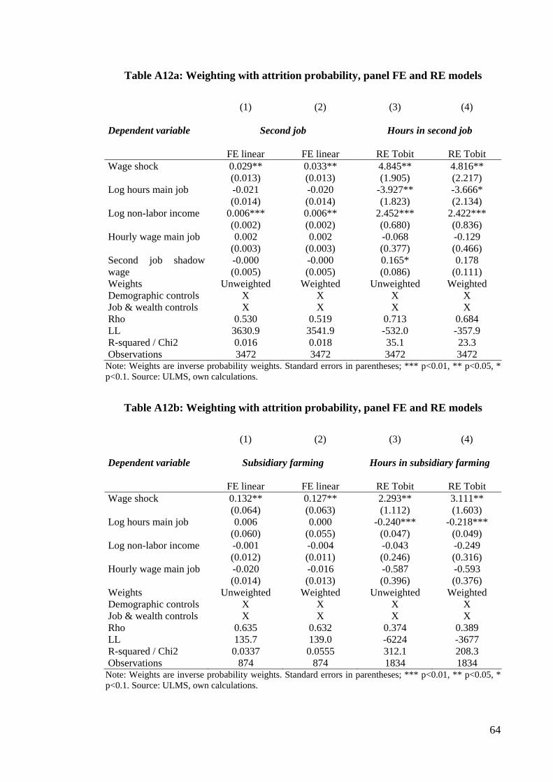
64

Table A12a: Weighting with attrition probability, panel FE and RE models

(1) (2) (3) (4)

Dependent variable Second job Hours in second job

FE linear FE linear RE Tobit RE Tobit Wage shock 0.029** 0.033** 4.845** 4.816** (0.013) (0.013) (1.905) (2.217) Log hours main job -0.021 -0.020 -3.927** -3.666* (0.014) (0.014) (1.823) (2.134) Log non-labor income 0.006*** 0.006** 2.452*** 2.422*** (0.002) (0.002) (0.680) (0.836) Hourly wage main job 0.002 0.002 -0.068 -0.129 (0.003) (0.003) (0.377) (0.466)

-0.000 -0.000 0.165* 0.178 Second job shadow wage (0.005) (0.005) (0.086) (0.111) Weights Unweighted Weighted Unweighted Weighted Demographic controls X X X X Job & wealth controls X X X X Rho 0.530 0.519 0.713 0.684 LL 3630.9 3541.9 -532.0 -357.9 R-squared / Chi2 0.016 0.018 35.1 23.3 Observations 3472 3472 3472 3472

Note: Weights are inverse probability weights. Standard errors in parentheses; *** p<0.01, ** p<0.05, * p<0.1. Source: ULMS, own calculations.

Table A12b: Weighting with attrition probability, panel FE and RE models

(1) (2) (3) (4)

Dependent variable Subsidiary farming Hours in subsidiary farming

FE linear FE linear RE Tobit RE Tobit Wage shock 0.132** 0.127** 2.293** 3.111** (0.064) (0.063) (1.112) (1.603) Log hours main job 0.006 0.000 -0.240*** -0.218*** (0.060) (0.055) (0.047) (0.049) Log non-labor income -0.001 -0.004 -0.043 -0.249 (0.012) (0.011) (0.246) (0.316) Hourly wage main job -0.020 -0.016 -0.587 -0.593 (0.014) (0.013) (0.396) (0.376) Weights Unweighted Weighted Unweighted Weighted Demographic controls X X X X Job & wealth controls X X X X Rho 0.635 0.632 0.374 0.389 LL 135.7 139.0 -6224 -3677 R-squared / Chi2 0.0337 0.0555 312.1 208.3 Observations 874 874 1834 1834

Note: Weights are inverse probability weights. Standard errors in parentheses; *** p<0.01, ** p<0.05, * p<0.1. Source: ULMS, own calculations.

65

Appendix B: Attrition Analysis

One potential source of bias in the ULMS stems from potential non-random

panel attrition. Sample attrition of the ULMS amounts to 19.5 percent for the entire

sample and 18.6 percent among those employed in 2003. For the purpose of this study it

is, however, interesting to analyze exits more broadly and to consider not only

individuals who leave the survey but also those who leave the employee status. A more

general analysis indicates that a substantial fraction of workers leave the employed

sample in the second year of the panel. As the goal is to track the causal effect from

labor market shocks on labor supply, it is important to investigate, in which labor

market states workers moved, and whether they potentially left jobs as a response to

wage uncertainty. From 2003 to 2004, the raw exit rate from dependent employment is

at 31 percent of the 2003 sample of dependently employed, while 19 percent newly

entered into this employment status. The substantial share of exits accounts for persons

who have reached pension age, engaged in entrepreneurial or professional farming

business, left their job temporarily in the reference week (e.g. for sickness reasons,

holidays or maternity leave) or left the labor force voluntarily (all together 9.3 percent)

or became unemployed (3.1 percent). The remaining 18.6 percent attrited from the

survey. Table B1 sheds light on the hypotheses that wage arrears might be correlated

with different kinds of exit behavior from dependent employment. Therefore simple

binary indicators are constructed which take on the value of one if an employed ULMS

respondent of 2003 left the sample for any of the given reasons, and zero otherwise.

These dummies are regressed on a wage shock indicator and some demographic and

regional characteristics employing a simple linear probability regression framework. If

attrition was perfectly random, we expect no statistically significant association between

the propensity to leave the sample and any right-hand side variables. This is rather

unlikely and indeed, we find that the demographics carry the expected signs. Women

and older respondents are less likely to leave the survey, while education matters for

unemployment. The results also suggest some specific geographic patterns of panel

attrition with inhabitants of the Centre and East region being more reluctant to drop out

of the panel. Most importantly, however, there is no significant positive or negative

correlation between the incidence of a wage shock in 2003 and subsequent exit from

employment or the survey.

Two approaches are used in order to investigate the impact of sample attrition on

the estimated second job holding responses: First, beside results stemming from a

66

balanced panel, the robustness of the results is shown with a maximal data sample

(Table A4 and Table A5). Second, the main results are re-estimated using inverse

probability weights (Wooldridge, 2002) that account for the predominant attrition of

specific subgroups (Table A11 and Table A12).36 Both procedures have very little

impact on the estimation results and confirm the robustness of the findings.

Table B1: Determinants of sample attrition, exit from the workforce and unemployment

(1) (2) (3)

(4)

Dependent variable: Sample attrition in t+1

Survey attrition in t+1

Unemploy-ment in t+1

Other exits from

employment in t+1

Wage arrear in t 0.006 -0.027 0.008 0.015 (0.027) (0.021) (0.010) (0.014) Age -0.001 -0.002*** -0.000 0.001** (0.001) (0.001) (0.000) (0.000) Years of education -0.008** 0.000 -0.003** -0.003 (0.004) (0.003) (0.001) (0.002) Female -0.017 -0.038** 0.009 0.022** (0.018) (0.015) (0.006) (0.009) Married 0.033* 0.022 0.002 0.001 (0.019) (0.015) (0.006) (0.011) Pseudo R-squared 0.062 0.132 0.049 0.030 Observations 3097 3097 3097 3097 Fraction of 2003 sample 28.9% 18.6% 3.1% 7.2% Note: The sample consists of all individuals who were eligible for re-interview in 2004. The estimation adopts a forward looking linear probability model. Cases (2), (3) and (4) are sub items of (1). All regressions control for regions. Standard errors in parentheses; *** p<0.01, ** p<0.05, * p<0.1. Source: ULMS, own calculations.

36 Inverse probability weighting proceeds in two steps, where in the first step an attrition indicator for t+1 is regressed on the covariates at t. In the second step, the fitted attrition probabilities are used as inverse weights.