
EFFECTS ON COST RIGIDITY AND INVESTMENT ...
155
INTERNATIONAL DIVERSIFICATION: EFFECTS ON COST RIGIDITY AND INVESTMENT CHARACTERISTICS Nancy Kangogo May, 2022 A dissertation submitted to the Kent State University Graduate School of Management in partial fulfilment of the requirements for the degree of Doctor of Philosophy
-
Upload
khangminh22 -
Category
Documents
-
view
2 -
download
0
Transcript of EFFECTS ON COST RIGIDITY AND INVESTMENT ...

INTERNATIONAL DIVERSIFICATION: EFFECTS ON COST RIGIDITY AND INVESTMENT CHARACTERISTICS
Nancy Kangogo
May, 2022
A dissertation submitted to the Kent State University Graduate School of Management in partial fulfilment of the requirements for the degree
of Doctor of Philosophy

ii
Dissertation written by:
Nancy Kangogo
Ph.D., Kent State University, 2022
MBA, Ohio University, 2005
MA, Ohio University, 2005
B. Commerce, Kenyatta University, 2002
Approved by:
Chair, Doctoral Dissertation Committee
Members, Doctoral Dissertation Committee
Accepted by:
Ph.D. Program Director
Graduate Dean,
College of Business Administration
iii
Table of Contents
List of Tables ............................................................................................................................................ iv
List of Appendices .................................................................................................................................... vi
Acknowledgements ................................................................................................................................. vii
CHAPTER 1: INTRODUCTION AND MOTIVATION .......................................................................................... 1
CHAPTER 2. LITERATURE REVIEW ................................................................................................................. 9
2.1 International Diversification ............................................................................................................... 9
2.2 International Diversification and Cost Rigidity ................................................................................. 10
2.3 International diversification and Investment Efficiency ................................................................... 15
2.4 International Diversification and R&D Intensity ............................................................................... 21
2.5 International Diversification and Uncertainty of Future Benefits from Investments ....................... 25
CHAPTER 3: HYPOTHESIS DEVELOPMENT ................................................................................................... 28
3.1 The Relation Between International Diversification and Cost Rigidity ............................................. 28
3.2 The Relation Between International Diversification and Investment Efficiency .............................. 35
3.3 The Relation Between International Diversification and R&D intensity ........................................... 41
3.4 International Diversification and Uncertainty of Future Benefits from R&D Investments .............. 45
CHAPTER 4. SAMPLE AND RESEARCH DESIGN ............................................................................................ 49
4.1 Sample ............................................................................................................................................... 49
4.2 Research Design ................................................................................................................................ 49
CHAPTER 5. RESULTS ................................................................................................................................... 61
5.1 Cost Rigidity- Results of Hypothesis Tests ........................................................................................ 61
5.2 Investment Efficiency - Results of Hypothesis Tests ......................................................................... 76
5.3 Research and Development Intensity -Results of Hypothesis Tests ................................................. 99
5.4 Uncertainty of Future Benefits from Investments - Results of Hypothesis Tests ........................... 108
CHAPTER 6. CONCLUSION ......................................................................................................................... 118
Appendices ................................................................................................................................................ 130
References ................................................................................................................................................ 145

iv
List of Tables
Table 1: Cost Rigidity Descriptive Statistics ................................................................................. 63
Table 2: The Effect of International Diversification on The Rigidity Of SG&A For Firms with Low
to Medium Levels of International Diversification ...................................................................... 64
Table 3: The Effect of International Diversification on The Rigidity of COGS For Firms with Low
to Medium Levels of International Diversification ...................................................................... 66
Table 4: The Effect of International Diversification on The Rigidity of Changes in Number of
Employees for Firms with Low to Medium Levels of International Diversification ..................... 67
Table 5: The Effect of International Diversification on The Rigidity Of SG&A Costs for Firms with
Higher Levels of International Diversification .............................................................................. 70
Table 6: The Effect of International Diversification on The Rigidity of Cost of Goods Sold Costs
for Firms with Higher Levels of International Diversification ...................................................... 72
Table 7: The Effect of International Diversification on The Rigidity of Changes in Number of
Employees for Firms with Higher Levels of International Diversification ................................... 74
Table 8 Panel A: Investment Efficiency -Descriptive Statistics .................................................... 77
Table 8 Panel B: Investment Efficiency -Correlations .................................................................. 78
Table 8 Panel C: Investment Efficiency -Variable Definitions ...................................................... 80
Table 9: Conditional Relation Between International Diversification and Investment for Firms
with Lower to Median Levels of International Diversification .................................................... 82
Table 10: Conditional Relation Between International Diversification and Investment for Firms
with Higher Levels of International Diversification ..................................................................... 86
Table 11: Deviation from Expected Level of Investment for Firms with Lower to Median Levels
of International Diversification: Under-investment Versus Normal Investment ........................ 90
Table 12: Deviation from Expected Level of Investment for Firms with Lower to Median Levels
of International Diversification: Over-investment Versus Normal Investment ........................... 92
Table 13: Deviation from Expected Level of Investment for Firms with Higher Levels of
International Diversification: Under-investment Versus Normal Investment ............................ 95
Table 14: Deviation from Expected Level of Investment for Firms with Higher Levels of
International Diversification: Over-investment Versus Normal Investment ............................... 97
Table 15: R&D Intensity Descriptive Statistics ........................................................................... 100
Table 16: R&D Intensity Correlations ......................................................................................... 101
Table 17: Effects of International Diversification On R&D Intensity-Fixed Effects .................... 104
v
Table 18: Effects of International Diversification On R&D Intensity: OLS Regressions ............. 105
Table 19: Uncertainty of Future Benefits from Investments -Descriptive Statistics ................. 110
Table 20: Effects of International Diversification on The Uncertainty of Earnings ................... 112
Table 21: Effects of International Diversification on The Uncertainty of Cash Flow from
Operations .................................................................................................................................. 115
Table 22: Effect of International Diversification on The Uncertainty of Sales Revenue ........... 117

vi
List of Appendices
Appendix 1: International Diversification Measure ................................................................... 130
Appendix 2: Variable Definitions ............................................................................................... 132
Appendix 3: Additional Analyses, Relation Between International Diversification and Cost
Rigidity in Firms with Low to Medium Levels of International Diversification .......................... 134
Appendix 4: Additional Analyses, Relation Between International Diversification and Cost
Rigidity in Firms with Higher Levels of International Diversification ......................................... 135
Appendix 5: Additional Analyses, Conditional Relation Between International Diversification and
Investment ................................................................................................................................. 136
Appendix 6: Additional Analyses, International Diversification and Deviations from Expected
Investment in Firms with Low to Medium Levels of International Diversification ................... 138
Appendix 7: Additional Analyses, International Diversification and Deviations from Expected
Investment for Firms with Higher Levels of International Diversification ................................. 140
Appendix 8: Additional Analyses- Relation Between International Diversification and R&D
Intensity for Firms with Low to Medium Levels of International Diversification ...................... 142
Appendix 9: Additional Analyses- Relation Between International Diversification and R&D
Intensity for Firms with Higher Levels of International Diversification ..................................... 143
Appendix 10: Additional Analyses- Effect of International Diversification on the Variability of
Future Benefits from R&D Investments ..................................................................................... 144

vii
Acknowledgements
First, I would like to thank God for the opportunity to pursue my doctoral program at
Kent State University. It has been a great blessing that enabled me to pursue my dream.
This dissertation is dedicated to my parents Mary Kangogo and the late Thomas
Kangogo Tegucho, and my sisters Lenah and Margaret. Without their assistance with my
upbringing, this journey would not have been possible. I thank my loving husband, Lewis, and
our kids, who have been very encouraging and patient with me throughout this journey.
I am eternally indebted to my dissertation committee, Rini Laksmana (Chair), Shunlan
Fang, and Murali Shanker for the time they invested in me and my success. Their enormous
support and guidance made this accomplishment possible.
I would like to acknowledge and appreciate the outstanding Kent State graduate faculty
that I had the pleasure to work with during my PhD program, including Pervaiz Alam, Mark
Altieri, Emmanuel Dechenaux, Arno Forst, Eric Johnson, Wei Li, John Rose, Drew Sellers, Wendy
Tietz, Jennifer Wiggins-Johnson, and Linda Zucca, among others.
A special thank you to my fellow accounting Ph.D. Students who were a great help and
company along the way.
1
CHAPTER 1: INTRODUCTION AND MOTIVATION
1. Introduction 1.1 Research Questions
Firms have been increasingly expanding their business activities across geographic regions
in pursuit of competitive advantages (Lu & Beamish 2004; Ramaswamy, 1995). Competitive
advantage result from economies of scale, access to resources, cost reduction, extension of
innovative capabilities, knowledge acquisition, location advantages and performance
improvements (Hitt et al., 1997). This research examines the relation between international
diversification1 and two factors: cost rigidity and investment characteristics. International
diversification can be defined as the expansion of a firms’ operation across country borders into
geographic locations that are new to the firm.
The research examines two questions. The first question is whether international
diversification is related to cost rigidity. Cost rigidity is an indication of the relative proportions
of variable-to-fixed costs ratio, and it is measured as the percentage change in cost for a
percentage change in sales revenue (Holzhacker et al., 2014; Banker et al., 2014). For example,
the percentage changes in selling and administrative expenses for a percentage change in sales
revenue.
The second question is whether international diversification affects investment
characteristics. I examine three investment characteristics: investment efficiency, uncertainty of
1 International M&A lead a level of international diversification depending on the number of foreign geographic
regions, sales per region among other factors.
2
future benefits from investments and R&D (research and development) intensity. R&D intensity
is used as a proxy for innovation.
1.2 Importance of the Research Questions
1.2.1 International diversification
This study’s focus on international diversification is due to four main reasons. First,
international diversification plays a pivotal role in corporate expansion and the strategic behavior
of large firms (Hitt et al., 1996) and has critical effects on firm outcomes relevant to global
competitiveness (Franko, 1989, Hitt et al., 1994) and firm performance (Lu and Beamish, 2004).
International diversification is therefore important for analyzing corporate strategy, goals, and
outcomes.
Secondly, the uniqueness of factors surrounding international diversification draws
further importance to this examination. International diversification presents unique benefits,
challenges, and costs due to the cross–border setting. A major source of benefits accrues to the
unique resource endowments and location-specific advantages in each host country (Lu and
Beamish, 2004). Internationalization provides opportunities to exploit imperfections in cross-
border use of firm assets (Caves 1989; Buckley, 1988), and improve knowledge base (Delios and
Henisz, 2000; Zahra et al., 2000). Alongside the opportunities, international diversification offers
great challenges (Child et al., 2001) and costs (Lu and Beamish 2004, Hitt et al., 1994).
Thirdly, there are trends towards increased international diversification despite
documented lower than expected performance and significant failures to realize the goals of the
3
international diversification (McGee, 2014). For example, over the past couple of decades there
has been dramatic increases in M&A activity and deal volume (Weber et al., 2013), as well as
huge increases in the number of deals (Shimizu et al., 2004). These trends are counterintuitive
given evidence that the rate of M&A failures is greater than 50 percent, with most of managers
reporting significant failures to achieve merger goals (Weber et al., 2013; Shimizu et al., 2004).
Lastly, the focus on international diversification is motivated by the voids in prior
literature. While the variation in firms’ performance following international diversification has
been widely documented in prior literature (e.g., Hitt et al., 1997), there are still voids in
understanding the reasons behind the variations in the findings. Studies document varying
patterns of association between international diversification and performance and other
measures of value. The mixed results have warranted calls by some scholars for the need to go
beyond investigation of the direct relations (e.g., Hitt et al., 2006). For example, studying
acquisition process and outcomes is an important step in understanding mergers and acquisitions
(Haspeslagh and Jemison, 1991; Child et al., 2001; Shimizu et al., 2004). This study heeds these
calls and aims to fill some of the voids in understanding the value creation effects of international
diversification by examining its interaction with cost rigidity and investment characteristics.
1.2.2 The relation between International Diversification and Cost Structure
In examining the relation between international diversification and cost structure, cost
rigidity is used as a proxy for cost structure. International diversification may affect cost rigidity
due to changes in firm resources and characteristics, the need to adjust to foreign territorial
conditions and changing market conditions (e.g., size, characteristics, opportunities, and threats).

4
An examination of the relation between international diversification and cost structure is
warranted by the pivotal role that cost structure plays in firm operations and ability to generate
profits. Cost rigidity is an important factor in firm performance because of its link to firm resource
commitment decisions in the face of adjustment costs (Banker et al., 2013). One of the main
reasons behind international mergers includes the potential benefits from economies of scale
and scope. A significant increase in productivity following mergers is from synergies. Synergies
arise from the sharing activities, and lumpy2 and intangible assets (Caves, 1989). Sharing affects
cost rigidity. Thus, there is an association between cost rigidity and the degree to which firms
gain from economies of scale and scope.
Evidence on the association between international diversification and cost rigidity is
useful to various stakeholders. Amihud et al. (2002) argues that cross-border operations lead to
increases in monitoring problems related to various factors including operating cost structure
among others. An examination of the relation between cost rigidity and international
diversification is useful to firms since it will shed light on firms’ success in adapting to changes in
geographic and other global market characteristics. Further, evidence on the relation between
international diversification and cost rigidity is useful for planning purposes. Management may
use such knowledge in increasing accuracy when estimating adjustment costs and potential gains
from economies of scale and scope.
2 Lumpy assets are those that represent a significant portion of total assets. Acquisition of lumpy assets involves significantly large cash or other financial resources.
5
1.2.3 International diversification and investment characteristics
International diversification may affect various investment characteristics including
investment efficiency, R&D intensity, and uncertainty of future benefits from investments.
International diversification may affect investment characteristics due its effects on various
factors. First, international diversification increases investment opportunities and organizational
goals. This is likely to affect investment efficiency, R&D intensity, and uncertainty of future
benefits from investments. For example, international diversification may lead to greater
investment efficiency due to an increased number of positive NPV projects available. Second,
international diversification increases organizational challenges from factors such as increased
demand fluctuations, institutional disruption (Kogut and Chang 1996; Allen and Pantzalis 1996),
information asymmetries and greater information processing costs (Kogut and Singh, 1988).
These challenges are likely to impact investment characteristics. For example, increased demand
fluctuations lead to increased uncertainty of future benefits from investments. Third,
international diversification fosters an environment that is more conducive to agency problems
due to increasing organizational goals, and greater information processing goals and information
asymmetries. These factors collectively affect firms’ investment strategies and choices which in
turn affect investment characteristics.
The importance of examining the relation between international diversification and
investment characteristics lie in role that the two factors and their interactions play in firm
operations and performance. Investment plays a critical role in firm performance. The quality
and quantity of investments relative to other firm factors is important as it affects long-term
6
operational sustainability and value creation through effects on revenue generation and cost
management.
Evidence on the relation between the degree of international diversification and
investment characteristics will also help illuminate puzzles presented by findings in prior
research. For instance, despite the strong evidence that diversification is value decreasing (e.g.,
Denis et al., 2002; Amihud and Lev; 1999), prior literatures document significant increases in
pursuit of global operations (e.g., Denis et al., 2002). Further, the results from the examination
of the relation between diversification and performance and other value measures are mixed.
This reinforces the importance of this examination since investment characteristics are related
to firm performance.
1.3 Contributions
The examination of international diversification and its relation to cost rigidity and
investment characteristics will provide insights into the variation in firms’ performance following
international mergers and acquisitions. This study heeds the calls in prior literature for evidence
on factors surrounding diversification (e.g., Hoskisson and Hitt, 1990; Rumelt, 1982; Haspeslagh
and Jemison, 1991; Child et al., 2001; Shimizu et al., 2004)). An examination of the relation
between international diversification and cost rigidity will contribute to the understanding of
corporate strategy and decisions. It will provide evidence whether firms are benefiting from
integration following international mergers and acquisitions. An examination of the relation
between international diversification and investment characteristics contributes to the

7
understanding of changes in firm performance following international diversification because
investment characteristics are linked to firm performance.
The evidence from this study will contribute to literature on international diversification.
There is scant literature examining the relation between international diversification and cost
rigidity as well as various investment characteristics. Despite the numerous studies on over-
investment (e.g., Richardson, 2006; Hubbard, 1998), there is scarcity of evidence on the link
between international diversification cost rigidity and investment efficiency3. This study is
valuable because it will provide various evidence from analyses based on a larger data set.
Evidence on the relation between international diversification and cost rigidity as well as
investment characteristics is beneficial to various stakeholders including management, investors,
and researchers. The evidence will be useful for managers evaluating risks, potential
opportunities, and value from international diversification, making decisions about international
diversification, and setting future corporate strategies. This knowledge could provide more
insights for estimating expected values from foreign mergers and generating better analyses and
decisions for international diversification pursuits.
The findings from this study are useful for investors assessing risk and choosing firms to
invest in. For example, investors may prefer to avoid investing in firms with a high level of
diversification if there is evidence that they exhibit high level of investment inefficiencies. The
findings from this study will provide valuable insights for researchers. For instance, relationships
between international diversification and cost rigidity and/or investment characteristics can be
3 Fuegebbayn et al (1997) examines the relation between international diversification and R&D intensity. The research however focuses only on 104 US firms with operations in the Middle East. Hitt et al. (1997) examines the relation between diversification and R&D intensity. The paper, however, uses only three years of data.

8
used in analyzing the documented evidence of variations in performance following international
mergers. The findings will provide leads into research areas that can narrow the research gaps in
documenting international diversification. For example, finding a positive correlation between
international diversification and uncertainty of future benefits may draw attention to research
into the specific causes leading to the uncertainty and potential remedies.
1.4 Research Approach
In addressing the research questions above, archival data will be used. The sample will
include US firms that are internationally diversified. The sample period will be for the years 1990
and 2018 Using a sampling period of two decades present an opportunity to examine the
variables of interest in the long run as some firms continue to increase their diversification levels
while others decrease it through divestitures or other means. Further, it facilitates comparisons
across periods using sub-samples. The restrictions to only US acquirers ensure a level of similarity
of the acquirer firms underlying factors such as management expertise and company resources
among others.

9
CHAPTER 2. LITERATURE REVIEW
2.1 International Diversification
International diversification (ID) is a strategy through which a firm expands the sales of its
goods or services across the borders of global regions and countries into different geographic
locations or markets (Hitt et al., 2007). International diversification is reflected by the number of
geographical markets and the firms’ degree of influence on the market. For instance, the firm’s
market share percentage in a country. Large-scale changes in the global environment over the
decades have made international diversification a very important strategic option for firms
seeking competitive advantage (Nachum and Zaheer, 2005) and value-creation opportunities
(Cartwright and Schoenberg, 2006). Hoskisson and Hitt (1990) present three market
imperfections that enable or drive firms to diversify4; firm resource heterogeneity, external and
internal firm incentives for diversification, and managerial incentives for diversification.
The imperfections also drive international diversification. International diversification
offers greater means for value creation through access to foreign stakeholders, resources, and
institutions (Hitt et al., 2006). Literature examining international diversification firm success in
achieving value creation document inconsistent results. Some studies documented positive
association between international diversification and various measures of firm value, such as
combined value of target and acquiring firms (Bradley et al., 1988), and market value (Ramirez-
Aleson and Espitia-Escuer, 2001). On the contrary, other studies found negative association
between international diversification and firm value (Berger and Ofek, 1995; Denis et al., 2002)
4 Authors argue imperfection is necessary for diversification; that is, diversification cannot be expected by firms acting in perfectly competitive markets.
10
and other related measures, such as earnings persistence (e.g., Riahi- Belkaoui, 2002; Riahi-
Belkaoui, 1998). Other studies document no impact of international diversification on total firm
value (e.g., Lins and Servaes, 1999).
Similarly, the results on the relation between international diversification and
performance are mixed. There is evidence of positive relationships (e.g., Geringer et al., 1989;
Delios and Beamish, 19995), and non-linear6 relationships (e.g., Hitt et al., 1997; Lu and Beamish,
2004; Capar and Kotabe, 2003; Ruigrok and Wagner, 2003; Lu and Beamish, 2001; Gomes and
Ramaswamy, 1999; Hitt et al., 1997; Lu and Beamish, 2004; Contractor et al., 2003; Quan and Li,
2002; Thomas and Eden, 2004; Qian and Li, 2002). The mixed results show that the association
between international strategies and both firm value and performance remain complex (Hitt et
al., 2006; Gomes and Ramaswamy, 1999). Further, it alludes to differences in other factors linked
to value creation and firm performance. The factors include cost and investment characteristics,
among other variables that are critical to success of internationally diversified firms.
2.2 International Diversification and Cost Rigidity
Cost rigidity is an indication of the relative proportions of variable-to-fixed costs ratio. It
is measured as the percentage change in cost for a percentage change in sales revenue
(Holzhacker et al., 2014; Banker et al., 2014). My examination of cost rigidity is motivated by the
fact that it is an attribute of cost behavior.7 Prior literatures specifically highlight the strategic
role of cost and its importance in strategic choices. For instance, Porter (1985) argues that cost
leadership is a main strategy to gaining competitive advantage.
5 Uses geographical scope instead of diversification. 6 Various forms of non-linear relationships 7 Cost behavior is the resource adjustment in response to changes in activity (Banker et al., 2014)

11
Cost is even more critical to internationally diversified firms. In fact, many motives for
international diversification are linked to cost factors. Motives for international diversification
include access to new resources, synergy from economies of scale and scope, performance
improvements (Hitt et al., 1997; Hitt et al., 2006) and exploitation of tax reduction opportunities
(Mudambi, 1995). All these motives are linked to firm cost factors or the objective of gaining
value through cost reduction. In line with these motives, Cullinan (2004) argues that some major
factors to consider when evaluating acquisitions include cost advantages and potential
improvements in costs that can be achieved. In line with the highlighted motives, international
diversification firms undergo changes and face unique factors that affect cost relationships.
Specifically, they experience changes in resources, firm internal capital market, among other
factors. In addition, they find opportunities for internalization, synergy realizations and efficiency
gains.
Arguments and findings in prior literature point to resource availability and the quest for
more resources as some of the main drivers of diversification. For instance, there are arguments
that diversification is driven by endowment of resources (Delgado-Gomez et al., 2004) and
availability of resources (Porter, 1987) including slack resources (Banker et al., 2011). RBV
(resource-based view or resource-based theory) has been widely used in diversification studies.
According to Rindova and Fombrun (1999: 694):
“Resource-based theory (Penrose, 1959; Barney, 1991) attributes advantage in an industry to a firm's control over bundles of unique material, human, organizational and locational resources, and skills that enable unique value-creating strategies (Barney, 1991).” Peteraf, (1993) notes that “heterogeneous resources create distinct strategic options for a firm that, over time, enable its managers to exploit different levels of economic rent. A firm's resources are said to be a source of competitive advantage to the degree that they are scarce, specialized, appropriable (Amit and Schoemaker, 1993), valuable, rare, and difficult to imitate or substitute (Barney, 1991).”
12
In the quest to gain resources, location is one of the core factors to firms undertaking
international diversification (Hymer, 1976). Location theory posits that multinational
corporations (MNCs) stand to achieve significant cost benefits because they can access cheaper
labor and material in overseas markets (Gomes and Ramaswamy, 1999). The variation in MNC
firm operating regions, offers MNCs the potential to take advantage of arbitrage opportunities in
factor cost differentials across multiple locations (Kogut, 1985). There is evidence that MNCs take
advantage of variation in country resource endowments such as availability of cheap labor (e.g.,
Kravis and Lipsey, 1982). Arbitrage opportunities facilitate changes to capacity and other factors
related to firm cost rigidity. There is evidence that firms shift their cost structure and tend to
have more labor intensive instead of capital-intensive operations in countries with lower cost of
labor (Kravis et al., 1978).
Extant literature commonly points to economics of internal capital markets as one of the
major advantages from diversification (e.g., Jones and Hill, 1998). International diversification
enables firms to increase their internal capital markets and their financing ability. International
diversification strategies such as acquisition, lead to an increase in both tangible and intangible
assets including goodwill, technical knowledge, and managerial skill set among others. This leads
to increases the ability to borrow as well as increase other resources. Greater resource availability
is particularly important, because a significant portion of firms’ tangible and intangible assets
that can only be acquired or increased in discrete and relatively large lumps (Caves, 1989).
Resources are crucial to cost decisions as capacity building and adjustments to manage overall
costs requires cash and other capital resources.

13
International diversification facilitates internalization. A firm can be viewed as an
internalized buddle of resources that can be allocated between product groups and markets
(Buckley and Casson, 1976). Literature point to internationalization as a means through which
internationally diversified firms gain efficiency (e.g., Hennart, 1982; Hitt et al., 1997). Firms are
prompted to enter international markets where transactions are not efficiently conducted
(Hennart, 1982) and gain from improving efficiency by internalizing acquired business units
(Caves, 1996). Moving transactions within the firm improves control, facilitates the dissemination
of information, and offers means of dispute resolution (Caves, 1996). Further, it facilitates
changes in management and agency related costs through reorganization of business units and
displacement of inefficient managers. Consequently, it may reduce agency costs relating to
subsidiaries.
Changes in resources and internalization promote efficiencies and synergistic gains.
Larsson and Finkelstein define synergy realization as “the actual net benefits (such as reduced
cost per unit, increased income) created by the interaction of two firms involved in a merger or
acquisition” (Larson and Finkelstein, 1999, p3). Lubatkin (1983) presents three main sources of
synergies8 including technical economies, pecuniary economies, and diversification economies.
Harrison et al., (1991) attribute synergy to two main sources; improved operating efficiencies
due to economies of scale or scope, and skill transfers. Similarly, internalization enables firms to
achieve corporate level synergy through marketing, R&D and other corporate level activities
8Lubatkin (1983) examines mergers in general, I expect similar patterns with international diversification.

14
(Yavitz and Newman, 1982) and overcome transaction difficulties in exploiting synergy through
the market forces (Jones and Hill, 1998)9.
Major sources of cost synergies include resource sharing (Hitt et al., 1994), resource
combinations (Marks and Mirvis, 2010). Firms combine resources following combinations and
share activities and resources such as personnel, plant and equipment, sales force, and
distribution channels for multiple products (Marks and Mirvis, 2010). For example, Procter and
Gamble uses the same physical distribution system for both diapers and paper towels. Sharing
promotes competitive advantage through either differentiation or lowered costs (Porter, 1996).
There are arguments and evidence that synergistic efficiencies increase market power over
competitors (Stewart et al., 1984; Montgomery, 1985).
Despite the factors discussed above which present opportunities for cost reductions,
firms diversifying internationally face cost trade-offs of doing business abroad (Hymer, 1976;
Caves, 1996). As US firms progressively diversify into foreign markets, they are likely to
experience increases in information impactedness10 due to greater physical, technological, and
psychic distance (Qian and Li, 2002; Markides, 1995; Habib and Victor, 1991). For example, for
firms diversify internationally, coordination, distribution, communication, and other related costs
will increase considerably and may exceed diversification gains (Hitt et al., 1997). Therefore, the
extent of gains from additional resources, internalization, improved efficiencies, and synergistic
9Jones and Hill (1998) identify that, economic benefits arise when internalization leads to decrease in production costs due to investment in specialized assets, decreased misallocation of resources and decreased need for complex contracts. 10 asymmetric distribution of information between parties to a transaction (Jones and Hill 1988)
15
gains is largely dependent on the firm’s ability to manage opportunities and control the costs of
international diversification.
2.3 International diversification and Investment Efficiency
Investment efficiency is critical to the success of internationally diversified firms.
According to Biddle et al. (2009) “a firm is investing efficiently if it undertakes projects with
positive net present value (NPV) under the scenario of no market frictions such as adverse
selection or agency costs. Thus, under-investment includes passing up investments with positive
NPV in the absence of adverse selection. Correspondingly, over-investment is investing in
projects with negative NPV.”
As a firm diversifies internationally there are various factors within the firm and its
operating environments that may affect investment efficiency. These factors center around their
effects on financial and other resources or other factors that have either direct or indirect impact
on firm investment activities. The following subsections discuss some of these factors.
2.3.1 Factors that encourage investment efficiency
Firms diversifying internationally experience various factors that are conducive to optimal
investing. These include increases in resources, tax incentives, managerial cultural diversity,
investment opportunities, market size, market needs, and opportunities for synergistic gains in
the global environment. International diversification leads to increases in financial and non-
financial resources that are critical to firm investment initiatives. The financial resources include
cash and debt capacity. A common argument in prior literature is that international
diversification increases debt capacity due to combination of businesses with imperfectly
16
correlated earnings streams (Ofek and Berger, 1995; Lewellen, 1971). In addition to increased
debt capacity, international diversification provides the flexibility for firms to borrow capital in
countries with lower borrowing costs (Denis, Dennis, and Yost, 2010) and it also creates
additional tax benefits through interest deductions (Berger and Ofek, 1995).
Tax provisions and incentives not only influences international diversification decisions,
but also MNE investment decisions. Tax advantages arise due to factors such as differences in tax
rates across countries and investment related tax incentives in various countries. Lower tax rates
and provision of infrastructure are important to investment decisions (Mudambi, 1995).
International diversification increases opportunities for tax avoidance using strategies such as
income shifting.
As firms diversify internationally, they can attract a more culturally diverse top
management team (Hitt et al., 1997). Managerial talent and skill pool are essential to the
formulation, implementation and monitoring of firm strategies including those related to
investments. Hoskisson et al. (1994) discusses that better knowledge of diverse market facilitates
coordination and the use of strategic controls.
International diversification increases potential investment opportunities arising from the
need to exploit market imperfections (Caves, 1989; Buckley, 1988). An increase in investment
opportunities emanates from the expansion into other geographical regions as well as other
sectors. Caves (1971) highlights that the initial impetus to a firm’s internationalization comes
from the opportunity to exploit market imperfections in the cross-border use of its intangible
assets. The opportunity to exploit market imperfections in the use of firm intangible assets is
17
indeed a main driver in most cases, even for firms with different initial motivations for
diversifying internationally.
Access to foreign markets raises the need for additional investments to take advantage
of the additional market opportunities. Specifically, additional investments are necessary to meet
the demands of the growing market as well as unique or modified demands of newer markets.
The need for additional investments is fueled by the fact that success in the global market relies
on innovations (Hitt et al., 1997). Further, customers expect higher quality products at lower
costs.
International diversification provides avenues for increased efficiencies and synergies.
Cross border mergers may speed new market access and promote globalization synergies
(Forsgren, 1989; Olie, 1990). Increased efficiencies may lead to accumulation of additional
financial and other resources that may be used for investments. Further, cross border mergers
and acquisitions can enhance combination potential in ways not available domestically. For
example, a firm may acquire an overseas target with complementary technology that is not
available locally.
2.3.2 Factors that may hinder optimal investment choices
Despite the various factors that are conducive to investment efficiency, MNEs face other
variables that may hinder optimal investment choices or encourage suboptimal investments.
Some of these factors include increases in excess cash, organizational complexity, information
asymmetry and coordination costs, diversity of investment options, agency problems, and
cross-subsidization.
18
International diversification leads increases in excess free cash due to direct increases in
cash and increases a firm’s internal capital market. Larger internal capital market creates greater
borrowing power and access to cash. There is consensus that overinvestment is prevalent
(Blanchard et al., 1994; Hubbard 1998; Bates 2005). Firms with free cash flows show greater
tendencies of wasteful expenditure (Jensen 1986; Stulz, 1990) and suboptimal acquisition choices
(Hartford 1999). The presence of excess cash in addition to other factors such as increasing
organizational complexity makes it conducive for investment inefficiencies.
International diversification increases organizational complexity due to greater
geographical, cultural, legal, communication, and other distances. These lead to greater
challenges and uncertainties in the international market (Child et al., 2001). Challenges and
foreign market factors will make it harder for firms to manage their investments. Kogut (1985)
notes that institutional and cultural factors hamper transfer of competitive advantage across
country borders. The complexities related to these factors may also make it harder for firms to
transfer knowledge on management of investments. Further, it may lead to sup-optimal
investment strategies, declines in value and eventual business unit failures. Ravenscraft and
Scherer (1989) attribute some of the declines in value following acquisitions to control loss owing
to complex organizational structures. Declines in value and divestures of acquired business units
may suggest presence of failures stemming from sup-optimal investment strategies.
Increasing organizational complexity may be worsened by a larger number of investment
options together with increasing number of managerial objectives, making it harder to choose
between various projects. Stultz (1990) argues that diversified firms make poor investments in
business units with poor investment opportunities. The problem may be more prevalent with
19
internationally diversified firms especially those facing an increasingly complex environment.
These issues are intensified by the higher governance requirements. There are arguments in prior
literature that governance exceeds management capabilities at high levels of product
diversification (Tallman and Li, 1996)11.
Diversifying into foreign countries increases information asymmetry and coordination
costs (Harris, Kriebel and Raviv, 1982). International diversification increases the number of units
across geographical regions as well as physical and psychic distance (Qian and Li, 2002). Greater
geographic dispersion increases coordination and management challenges (Hitt et al., 1994).
Other factors such as cultural, psychic distance, legal, and communication barriers, heighten
coordination costs. Some prior literature further document that diversification creates
inefficiencies. For example, Chandler (1977) points to additional inefficiencies created by
additional managerial levels charged with coordinating divisions in diversified firms. Along the
same line, as international diversification increases, firms may venture more into investments
that are not related to its core business. This may lead to significant negative synergies across
the business segments and misallocation of management time and other resources (Jayasuriya
and Shambora, 2009). Anecdotal evidence links increasing geographical diversification to
significant cost increases. For example, Geringer et al. (1989) discuss that managers
communicated those costs began to escalate as their firm’s geographic market became
increasingly broad. A significant part of increasing costs is due to coordination and
communication challenges.
11 Thou Tallman and Li’s (1996) argument is based on product diversification, I expect international diversification will present similar and greater challenges to management.

20
Like other corporations, firms diversifying internationally face agency problems. Based on
agency theory and moral hazard models, managers pursuing their personal welfare may tend to
make investments that are not consistent with maximizing shareholder value (Jensen and
Meckling, 1976). For instance, they may invest in negative NPV projects. Managerial empire
building is widely documented in prior literature as one of the important drivers of diversification.
For instance, Jensen (1986) argues that even though diversification may be inefficient, managers
choose to diversify when they have free cash flow in order to build empires (Jensen, 1986). On a
similar note, Doukas and Lang (2003) indicate that the negative valuation effects of foreign direct
investment activity of US firms seem consistent with empire building and over-investment.
Agency problems may be greater in international diversified firms due to greater
monitoring difficulties, information asymmetries, and availability of free cash flows, among other
factors. Managers with more free cash flows due to effects12 of international diversification
undertake more investments in negative NPV projects (Jensen, 1986). Evidence shows that the
problem is more prevalent with diversification13. For example, Rajan, Servaes and Zingales (2000)
model and test the prediction that diversity in resources and opportunities increase flow of
resources toward the most inefficient division, leading to more inefficient investment and less
valuable firms.
International diversification may provide avenues for cross-subsidization- a factor that
is detrimental to value creation (Meyer et al., 1992). The evidence of well performing segments
12 Effects such as increase in firm size and greater borrowing ability among others. 13 I expect that the problem would generally be worse with international diversification (relative to diversification within one country) due to greater complexities, geographic distance, firm size, and information asymmetry among others.
21
subsidizing underperforming segments in diversified firms (Lamont, 1997), suggests that
diversification may have effects on investment efficiency. Cross-subsidization may affect
investment behavior through various means. For instance, high performing units will be less
motivated to maximize their performance when their surplus is used to support underperforming
divisions. Meyer et al. (1992) found evidence that some profitable segments did not strive as
hard as they might for higher earnings because their surplus was transferred into money losing
operations. These tendencies would foster under investment among well performing divisions
that have positive NPV investment options.
2.4 International Diversification and R&D Intensity
R&D intensity is a proxy for innovation, and it is measured as the ratio between R&D
expenditure to total number of employees (Hitt et al., 1997; Hill and Snell, 1988). R&D is an
important determinant of firm performance (Hitt et al., 1997; Jensen, 1986), because it affects
process and product innovation. There are findings in prior literature that R&D investments are
positively correlated with various performance measures. There is evidence of positive relation
between R&D investments and profitability (e.g., Severn and Laurence, 1974) and firm
productivity (Hill and Snell, 1989).
Process and product innovation are crucial to gaining competitive advantage in
international markets (Porter, 1991; Hitt et al., 1994; Hitt et al., 1997). This reinforces the
importance of examining the relation between international diversification and R&D
investments. Internationally diversified firms have various incentives for innovations (Hitt et al.,
1994) and other factors that may encourage investments in R&D. The incentives center around
the need to adapt and take advantage of market opportunities and investment opportunities in

22
international markets. International markets come with increases in demand for high quality and
low cost (Prahalad, 1990). In addition, companies may experience additional push from markets
demanding unique products or products tailored to the specific regions.
In addition to creating incentives, international diversification leads to increases in
resources-a critical element to R&D investments. International diversification may be necessary
to generate enough resources for large scale R&D operations (Kobrin, 1991). Resources are
directly used in R&D investments. Further, greater financial and other resources enable firms to
internalize and integrate their global operations, which is also pivotal to R&D investments. There
is evidence that US firms that have achieved significant integration are able to retain their
innovative abilities (Kotabe, 1990). Retention of innovative abilities may suggest existence of
significant R&D investments. Along similar lines, some prior literature document positive relation
between international diversification and other factors related to R&D. For instance, Zahra et al.
(2000) found that international diversification improves technological learning, which in turn
fosters innovation, differentiation, and market expansion speed.
Despite the incentives and factors that may foster investments in R&D, there are others
that may hamper investments in R&D. These factors include the use of acquisition as an
alternative to R&D investments, appropriation of innovations, decreased focus on specific
business units, and challenges with coordination and extending skillset and expertise across
countries.
Prior research finds evidence that firms may make tradeoffs between various strategies
(Hoskisson and Hitt, 1990; Geringer et al., 1989) including acquisitions and R&D investments. For
example, Banker et al. (2011) finds that firms with a high degree of diversification are likely to

23
innovate through acquisition, rather than through investment in R&D. Large firms often acquire
smaller firms due to the target’s technical and other capabilities. Acquisitions therefore help to
increase technical and other knowledge resources and may thus decrease the need for additional
R&D investments.
Kotabe (1990) argues that international diversification facilitates appropriation of
innovations. With appropriation, firms can apply competencies from their local market to
international markets to increase their performance (Bartlett and Ghoshal, 1999). Some of the
competencies emanate from R&D investments from the host country. In addition, international
diversification enables firms to tap into selective advantages of other countries (Porter, 1990)
and use it to fill the increasing market needs in other regions. Appropriation of innovations and
R&D resources decreases the need for additional R&D investments. In line with the preceding
arguments, Banker et al. (2011) finds that IT firms with a high degree of diversification14 tend to
innovate through acquisition rather than R&D.
In a firm with multiple business units, no single unit may feel responsible for maintaining
a viable position in core products nor be able to justify R&D investments required to build
leadership in their products (Prahalad, 1990). This situation is particularly critical in the context
of international diversification because such diversification is likely to decrease the weight of
specific business units given the increase in the number of business units. A company’s focus on
its core products is essential to its competitiveness and survival. Therefore, the increase in
14 Thou Banker et al. (2011) focused on diversification in general, I expect the same tendencies with international diversification.

24
business units due to international diversification may lead to decreases in the R&D investment
for each core product.
Greater geographic dispersion presents coordination and communication challenges
amongst internationally diversified companies. With greater dispersion, coordination and
communication barriers arise (Porter, 1990; Hitt et al., 1997). Dispersion may hamper
collaboration among divisions in various regions due to coordination, communication, and other
related challenges. Yeoh (2004) finds that geographic diversity of exports has negative effect on
technological learning. This may be an indication of coordination and communication challenges
on innovations.
There may be limits to the transferability of firm knowledge and its acceptance across
regions (Rugman and Verbeke, 2004). Differences in legal and cultural characteristics across
nations exacerbate difficulties when adapting to foreign markets and impose transferability
limits. In addition to limiting transferability, the differences may also limit firm ability to take
advantage of resource disparities across geographic regions. These differences reiterate the need
for additional investments in innovations and other capacities. Limited ability to transfer and
apply managerial and other skill may hamper innovations, because skill and expertise are critical
in a firm’s endeavors to innovate and remain competitive.
Extant literature documents evidence that large investments often fail in new areas
because of lack of appropriate management and production. Caves (1989) discusses that the
evidence of some divestures following acquisitions, is consistent with multiple business having
certain skills, controls and structures that work on a subset of firms, but crumble when applied
to new areas. He further argues that divestures may be the result of insufficient investment in
25
technical and other forms of learning to gain value from the acquired business units. This points
to the need for additional investments to achieve the appropriate knowledge and structures to
increase competitiveness as the market becomes more complex and diversified. Investments in
R&D play a pivotal role in this endeavor.
2.5 International Diversification and Uncertainty of Future Benefits from Investments
Firms, standard setters, and other users of financial information are concerned about the
likelihood that future benefits will be realized from investments and other resource outlays. For
instance, FASB uses the degree of uncertainty of future benefits as a criterion of determining
whether a cost should be expensed or capitalized (Statement of Financial Accounting Standards
No. 6, 1980). In this study, the uncertainty of future benefits from investment is measured by
future variability in value from investment (Kothari et al., 2002; Asdemir et al., 2012)15.
Ravenscraft and Scherer (1989) found evidence that, except for mergers involving pooling of
interest between firms of relatively similar sizes, the acquired business units experienced decline
in performance. They point to investment changes as possible causes of the documented decline.
This highlights the importance of investment quality to the performance of internationally
diversified companies.
One objective of this study contributes to the understanding of the variations in the
performance of internationally diversified firms. The examination of the uncertainty of future
benefits from investments by internationally diversified firms provides insights on the link
between firm inputs and financial outcomes, a lens into firms’ global effectiveness and value
15 In these papers, future variability in value is proxied by standard deviation of future earnings, sales revenue, and operating cash flows.

26
creation. Uncertainty in future benefits from investments is an important indicator of investment
quality. A common argument in prior literature is that international diversification results in
combination of imperfectly correlated earnings streams (Ofek and Berger, 1995; Lewellen, 1971).
The evidence of reduced risk of revenue stream variability (e.g., Hisey and Caves, 1985; Hwang
and Burgers, 1993) among diversified firms coincides with this argument.
Due to its critical role in firm performance and survival, R&D has received considerable
focus in the investment literature. R&D is an increasingly important productive input (Aboody
and Lev, 2000). The findings reiterate the central role that R&D plays in organizational growth
and performance. For instance, there is documented evidence that R&D expenditure is
associated with future performance (e.g., Deng and Lev, 2006) and market values (e.g., Hirschey
1982; Hirschey and Weygandt, 1985; Shevlin, 1991). Further, prior studies have documented that
the market assigns value to R&D activities (e.g., Lev and Sougiannis, 1996; Deng and Lev, 1997).
Despite the association between R&D and variables associated with firm value, FASB
requires that R&D expenses to be expensed immediately (SFAS No. 2) because of the high
uncertainty of future benefits from R&D investments. In SFAS No. 4, FASB specifically points to
the high degree of uncertainty of R&D expenditures in providing future benefits. The uncertainty
of R&D expenditure is especially greater for R&D intensive industries (Amir et al., 2007; Asdemir
et al., 2012). Comparing earnings variability of R&D versus that of capital expenditures, Kothari
et al. (2002) documents that the variability of R&D is about three-to-four times as large as that
of capital expenditures (Kothari et al., 2002, p. 357).

27
For manufacturing firms, while R&D may not constitute significant portion of the
investment outlays16. However, R&D remains a critical component to firm success. Amir et al.
(2007) argues that the capitalization of R&D should only be allowed in CAPEX-intensive firms
because the volatility of subsequent operating profitability is equally influenced by R&D and
CAPEX. There is evidence of significant correlation between R&D and future earnings (e.g.,
Kothari et al., 2002).
For internationally diversified firms R&D and other factors play a role in determining the
relation between the investments and uncertainty of future benefits. These factors include
geographical dispersion, market characteristics (e.g., similarity to home market), infrastructure
quality, and distribution networks among others.
16 I expect that investments in R&D are lower because they are mostly aimed at relatively small product and process improvements.
28
CHAPTER 3: HYPOTHESIS DEVELOPMENT
3.1 The Relation Between International Diversification and Cost Rigidity
Prior literature does not provide conclusive evidence on the relationship between
international diversification and cost rigidity. There are no studies that specifically delve into the
relative changes in variable versus fixed costs as firms diversify internationally. However, extant
literature present various arguments that are directly or indirectly related to the relationship
between international diversification and cost and cost rigidity. Ex-ante, there is consensus that
cost advantages is one of the drivers of international diversification (Hitt et al., 1997; Kogut,
1985). Ex-post, international diversification will drive changes in cost due to several factors that
differ across phases as firms expand from low levels through higher levels of international
diversification17. Through international diversification phases, firms face various factors
including, location choices, changes in resources, synergy and economies of scale, integration,
organizational learning and changes in governance, and environmental complexity.
3.1.1 Low to moderate levels of international diversification
In the initial phases of international diversification18, firms consider location choice due
to its pivotal role on costs, among other factors (Hitt et al., 1997). Location choice literature posit
that firms choose locations based on psychic, cultural and geographic distance (Papadopoulos
17 This study follows the approach Hitt and Middlemist (1978) and Hitt et al. (1997) in measuring level of international diversification. I use an entropy measure of international diversification that factors both the number of global market regions and the relative importance of each global region. The specific calculation is presented in eq. (1) in chapter 4. Based on the measure, firms are categorized into low-to-medium international diversification subgroup if they have an international diversification score(measure) of less than 0.30. Firms with a score of 0.30 and above are classified as categorized into the higher international diversification group. 18 Location factors are also considered in further international expansion decisions
29
and Dennis, 1988). Research has found support for market familiarity concept where firms give
preference to familiar markets (e.g., Davidson, 1983). In line with this prediction, David (1980)
finds that US firms prefer to start with Canada and the U.K when venturing into global expansion.
Similarly, Hisey and Caves (1985) predicts that firms prefer expanding in countries where they
already have operations due to experience in host country. These expansion choices help firms
to limit costs such as fixed cost related to finding new sites of operations (Hisey and Caves, 1985).
This is because familiar markets have similar distribution, administrative and marketing
characteristics, which enables appropriation of home country competencies and cost reductions
(Gomes and Ramaswamy, 1999, p 176). Expansion into familiar markets facilitates activity sharing
which may facilitate decreases in fixed costs and cost rigidity.
Location choice also affects firms’ abilities to take advantage of resource availability and
resource costs (Caves, 1989). U.S firms’ initial expansion into familiar markets such as Canada
and U.K, may not create significant differences in labor abundance and cost- a critical
manufacturing variable cost factor. Companies are therefore not likely to have significant shifts
towards a higher variable -to-fixed cost approach19. However, as they continue to medium levels
of diversification, they gain incremental opportunities to take advantage of resource availability
and prices. For instance, firms may adopt approaches substituting capital for direct labor due to
abundance and lower cost of human resources in foreign countries (Kravis and Lipsey, 1982). This
may move the company towards lower cost rigidity.
Another consequence of increased firm size is the increase in power over suppliers and
other supply chain participants. The impact of increased firm power on cost rigidity is unclear
19 Shifts would occur if firms changed their capital and labor ratios.
30
because it may create opportunities to decrease both variable and fixed costs. For example,
purchasing fixed assets at lower cost and variabilization of fixed costs would decrease cost
rigidity. Lower cost of raw materials could reduce variable costs relative to fixed costs and cause
increases in cost rigidity20.
Extant literature highlights that the desire for synergistic gains and economies of scale
affects initial and subsequent international expansion decisions (e.g., Larsson and Finkelstein,
1999, Lubatkin, 1983; Chartejee, 1986). Synergistic gains are attributable to improved operating
efficiencies (Jensen, 1993) due to economies of scale or scope, and skill transfers (Harrison et al.,
1991), among other factors. At lower to moderate levels of international diversification21, firms
may significantly benefit from sharing asset advantages and resources such as distribution,
marketing, and administrative resources (Gomes and Ramaswamy, 1999) across more markets.
Low to moderate international diversification is specifically conducive to asset sharing,
synergistic gains and other related benefits because of relatively higher business and market
similarity (due to related diversification). Hisey and Caves (1985) note that firms will tend to
pursue related diversification until the point at which marginal cost starts to exceed returns. At
which point they branch out to new product or geographic region. Sharing assets is likely to lead
to relative22 decreases in fixed costs. I expect relatively larger decreases in fixed costs because
sharing in activities that significantly drive fixed cost including administrative and marketing
human resources23 as well as production facilities among others. For example, when a U.S firm
20 BCG defines variabilizations as the conversion of fixed costs into variable costs. For example, selling fixed assets back to the manufacturer and renting them at a fee that varies with revenue or usage 21 Firms with low-to-moderate levels of international diversification are those with an international diversification that is less than the median. Similar to Hitt et al. (1997), I find that median is approximately 0.3(rounded). 22 Fixed cost relative to variable cost 23 For example, sharing of managers and other personnel will help decrease overall salaries.
31
expands to Canada, divisions in the US and Canada can share distribution resources such as
trucks, personnel, and other resources. This leads to decreases in the proportion of fixed costs24
relative to variable costs. Variable costs will generally increase in proportion to the increased
activity level. Such changes would decrease cost rigidity.
Organizational learning plays an important role in firm success (Barkema and Vermeulen,
1998; Hitt et al., 1994). Given challenges in the global environment, experience and
organizational learning are particularly critical as firms expand internationally. Firms at lower
level of international diversification encounter liabilities of newness and foreignness. These firms
tend to have low product diversification. As firms expand, moving from low to medium levels of
international diversification, they have experiential learning curve on establishment and running
of subsidiaries (Hisey and Caves, 1985). Increased knowledge and experiential learning enable
firms to better manage and reduce relative25 fixed and variable costs. However, the impact on
cost rigidity is unclear given the lack of evidence on the relative changes of fixed and variable
costs.
3.1.2 Higher levels of international diversification
Hitt et al. (1997), describes high diversification firms as those with an international
diversification score above 0.30. International diversification score is calculated based on
number of sales regions, as well as sales amount per region. For each firm, an increase in the
number of sales regions and/or activity on a sales region(s) leads to a higher international
24 Such as depreciation expense and salaries. 25 In relative terms such as per unit basis or in comparison to activity level.
32
diversification score. Beyond medium levels of international diversification26, firms still face the
factors above; that is, location factors, synergistic gains, experiential learning, market complexity
among others. However, firms face more challenges that affect the nature and effects of these
factors and cause significant increases in costs. For instance, cross-border mergers may impede
integration and coordination needed to realize synergies because of geographic distance as well
as legal, financial, psychic, and other country differences (Marks and Mirvis, 1993; Hitt et al.,
1997; Qian and Li, 2002). Once firms enter unfamiliar territories requiring major reconfiguration
of internal processes, structures, and mechanisms, the costs of internalization dramatically
increase to exceed benefits (Ruigrok and Werner, 2003).
As firms expand from medium to higher levels of diversification, there are greater
opportunities to take advantage of arbitrage opportunities in factor cost differentials across
multiple locations (Kogut, 1985). This is especially the case as firms expand into less developed
countries. Early research finds evidence that firms used more labor-intensive technologies in
countries with cheaper labor cost (Kravis and Lipsey, 1982). Shifts from capital-intensive towards
labor-intensive approaches, leads to greater increases in total variable cost relative to the
increases in total fixed costs hence a decrease in the proportion of fixed costs relative to variable
costs27. For such shifts would lead to disproportionately higher increases in total direct labor cost
relative to increase in total depreciation costs. Hence leading to decreases in cost rigidity.
26 International diversification is calculated based on number of sales regions, as well as sales regions. Increase in the of sales regions and/or activity on a sales region. Such that firms operating in a greater international diversification score. 27 Or relative to total cost.
33
Despite available opportunities to benefit from lower labor cost and abundance of other
resources, when MNCs expand beyond optimal level of international diversification, control and
coordination costs, cultural and other operating environment dissimilarity is expected to lead to
higher costs that exceed potential returns to multinational growth (Gomes and Ramaswamy,
1999). For instance, greater geographic and other dispersion which makes it more challenging to
share assets such as production facilities, distribution networks, and personnel among others
(Hitt et al., 1997). This is escalated by differences in customer tastes and increasing product
diversification and less focus which similarly creates a need for additional and specific assets.
Difficulty sharing assets makes it necessary to increase such assets in multiple regions or
countries. An increase in assets such as productions facilities and equipment among others is
likely to cause greater increases in fixed costs hence leading to an increase in cost rigidity.
Differences in legal and other regulatory systems will create significant governance
challenges. Increasing firm size and the limits to applicability of managerial skill to certain
countries, regions or business units worsens governance challenges. In addition, with increasing
differences between home country and foreign market, firms will face greater challenges
purchasing and installing facilities (Lu and Beamish, 2004). Governance challenges and
complexities necessitate hiring of foreign managers, leading to salary increases among other
costs. I expect that this would lead to greater increases in fixed cost relative to variable costs
hence leading to greater cost rigidity.
Expansion into new regions or territories, changes the operating environment of the firm
including uncertainty and risk levels (Lee and Caves, 1998). Uncertainty and risk levels are pivotal
factors to manager decisions including those linked to cost rigidity. Prior literature examining the
34
relationship between uncertainty and cost rigidity yielded inconclusive results. Using hospital
data, Kallapur and Eldenburg (2005) find evidence that hospitals increased cost flexibility
(increased cost rigidity) when they faced greater uncertainty. On the contrary, Banker et al.
(2014) found evidence of positive association between uncertainty and cost rigidity (higher fixed-
to-variable costs). Their findings coincided with their arguments that when firms are faced with
uncertain demand, they increase their capacity, to take advantage of future high demand28.
Increasing capacity leads to an increase in fixed cost hence a greater cost rigidity.
In sum, the relationship between international diversification and cost rigidity is not clear.
This is due multiple conflicting direction of effects of factors that affect cost making the overall
direction less clear. Further, the evidence on magnitudes of changes in fixed and variable costs
as firms diversify internationally is unclear. The overall changes in cost rigidity will depend on the
cost shifts directions and magnitudes as firms diversify internationally. At lower to medium levels
of international diversification, expansion into relatively similar markets29, activity sharing,
synergistic gains, among other the factors appear to point more towards decreasing cost rigidity.
This is because these factors lead to lower increases in total fixed costs relative to the increases
in total variable costs. I therefore predict a lower cost rigidity at low to medium levels of
international diversification. With higher international diversification, market complexity,
difficulty sharing activities, other factors within the MNCs and their operating environment are
likely to necessitate greater capital outlays30, leading to greater increases in total fixed costs
28 Higher proportion of fixed costs leads to greater gains in times of high demand. 29 Expansion into similar countries facilitates greater asset sharing and likely to cause a smaller increase in fixed cost relative to the increase in variable costs. 30 Fixed costs for setting up production facilities, infrastructure, machinery, and equipment, among others.
35
relative to increases in total variable costs. Thus, it may lead to increasing cost rigidity. I therefore
predict higher cost rigidity at higher levels of international diversification. The following
hypotheses below capture these predictions:
H1a: At low to medium levels of international diversification, there is negative
association between international diversification and cost rigidity.
H1b: At high levels of international diversification, there is positive association
between international diversification and cost rigidity.
3.2 The Relation Between International Diversification and Investment Efficiency
Despite expansive literature on both international diversification and investment, there
is no literature that I am aware of that examines the relationship between international
diversification and investment efficiency. It is plausible that international diversification has both
direct and indirect effects on overinvestment and underinvestment. The extend of the effects of
international diversification on investment efficiency, and directions of these effects remains an
open question. The relation between international diversification and investment efficiency
stems from the changes in various factors both within the firm and its environment as the firms
diversify from low-to-medium levels of international diversification to higher levels of
international diversification. The factors include investment opportunities, incentives, resources,
knowledge and experience, and organizational and environmental complexity, uncertainty,
governance challenges, agency problems, among others. At low-to-moderate levels of
international diversification, these factors are more likely to foster investment efficiencies.
36
3.2.1 Low-to-medium levels of international diversification
At low-to-moderate levels of international diversification, availability of investment
opportunities is a major incentive for initial and continued international diversification.
Operations in foreign countries will generally lead to increase in the quantity and quality of
investment opportunities. The increase in investment opportunities is driven by the need to take
advantage of a larger and varied market and exploit market imperfections (Buckley, 1988).
Expansion into foreign markets will encourage investments in R&D since firms can diffuse
innovations to a larger market before competitors either copy the technology or come up with
competing technology or product. Barlett and Ghoshal (1989) argues that MNEs (multinational
enterprises) expect benefits from ability to hasten new product development and introduction.
This may encourage investments hence reduce underinvestment problem. The availability of
investment opportunities is likely to decrease underinvestment and overinvestment because of
the availability of better investment alternatives.
Incentives available to firms diversifying internationally fuel further increase in
investment opportunities. For instance, in a bid to boost investment inflows from foreign
countries, some nations offer incentives. This may be in the form of tax breaks, lower import, or
export duties, among others. Incentives not only increase availability of better investment
projects, but also mitigate both underinvestment and overinvestment. In the pursuit of
investment opportunities and taking advantage of investment incentives, firm access to
resources plays a critical role.
Availability of resources including cash, is pivotal to both international diversification and
investment activities. Resource availability is not only an incentive to diversify internationally,
37
but it fuels continued international diversification (e.g., Banker et al., 2011; Delgado-Gomes et
al.,2004). Other incentives for international diversification including economies of scale (Hitt et
al., 1997), arbitrage in factor cost differences (Kogut, 1985), and increased efficiency (Berger and
Ofek, 1995), synergy and efficiency helps to enhance firm resources (Forsgren, 1989). The greater
endowment of resources and additional resources acquired by internationally diversified firms
are conducive to investment activity. I therefore expect decreases in underinvestment due to
resource factors. Overall effects of resources on investment efficiency are subject to factors such
as managerial knowledge and skill.
As firms diversify internationally, knowledge is critical to both the success of the
international diversification and investments. Managerial knowledge is pivotal to firm success in
harnessing available investment opportunities and incentives, and to better utilization of
resources. During earlier stages of international diversification, firms face newness and
foreignness (Lu and Beamish, 2004) and are prone to problems managing international
diversification efforts. However, as firms diversify from low to medium levels of international
diversification, experiential learning (Hitt et al., 1997) leads to improvements. Evidence of better
performance at medium levels of diversification (Hitt et al.,1997) coincide with these
observations. Increase in experiential learning and related improvement in managerial skill is
conducive to investment efficiencies. Therefore, I expect increases in investment efficiency as
firms progressively advance from lower to medium levels of international diversification.
Based on the arguments and findings discussed above, I expect the factors above to lead
to both a decrease in under-investment and over-investment. I therefore posit that lower to
medium levels of international diversification will be positively associated with investment

38
efficiency as manifested through lower over-investments and lower under-investment. The
following hypotheses capture this prediction:
H2a: At lower to medium levels of international diversification, international
diversification is negatively associated with over- investment.
H2b: At lower to medium levels of international diversification, international
diversification is negatively associated with under- investment.
3.2.2 Higher levels of international diversification
Despite the pointers towards greater investment efficiency as firms diversify
internationally, there are barriers to achievement of outcomes. These barriers are more
pronounced at higher levels of international diversification. First, as firms progressively expand
beyond medium levels of international diversification, internal and external complexity increases
(Ravenscraft and Scherer, 1989). Internal complexity increases due to the increasing company
size and increasing number of divisions or business units (Chandler, 1977). Increasing firm size
leads to greater information asymmetry, and information processing and coordination costs
(Harris et al., 1982; Porter, 1990). Apart from greater complexity, firms at higher levels of
diversification are more likely to diversify into other industries. There is consensus that in most
cases industrial diversification destroys value (e.g., Jensen, 1986). A common source of value
destruction is suboptimal investment quality.
Secondly, uncertainty will significantly increase as firms expand into less familiar
territories (Child et al., 2001). Uncertainty will be higher at higher levels of international
diversification because at such levels, firms expand more into countries with greater geographic,
39
psychic, cultural, legal distance31. Several researchers show that irreversibility of investments
causes risk neutral firms to reduce current investments in the presence of uncertainty (e.g.,
Bernanke, 1983; Pindcyk, 1988; Dixit and Pindyck, 1994). Hence, I expect that firms at higher
levels of international diversification may hold back on some investments due to higher levels of
uncertainty. This is likely to increase under-investment.
Third, increasing complexity, increasingly varied market and uncertainty leads to greater
challenges with governance (Hitt et al., 1994). For instance, it is tougher for management to
evaluate investment options and to decide on investments to pursue. Governance challenges
coupled with greater information asymmetries is likely to affect information and decisions
related to investments. For instance, it is more challenging to evaluate business units and their
respective investment projects, making it harder to choose optimal investment choices.
Lastly, complexity and information asymmetry may fuel agency problems (Jensen and
Meckling, 1976) through various means. For example, complexity and information asymmetry
may be conducive for empire building (Doukas and Lang, 2003) as managers seek to acquire more
power, prestige, and compensation (Stulz, 1990; Jensen and Murphy, 1990). Managers may
pursue suboptimal projects in efforts to increase their business units or segments despite the
existence of better projects in other divisions. Managers with greater power or influence may get
priority in funding with less weight being placed on the viability of the alternative investments
across business units. In fact, information asymmetry may create room for cross subsidization,
where better performing business units subsidize worse performing units. Investment
31 There is evidence that firms prefer to first expand into more familiar territories first and expand into less familiar territories later (e.g., Gomes and Ramaswamy, 1999; Ruigrok and Wagner, 2003)

40
inefficiencies from the aforementioned factors is greatly compounded by greater access to cash
(Jensen, 1986) and other resources which are more available to firms that have a higher level of
international diversification. Greater levels of over-investment and under-investment would
manifest investment inefficiencies.
As discussed above, higher levels of international diversification may be detrimental to
investment efficiency. I therefore predict that higher levels of international diversification will be
associated with decreases in investment efficiency which is depicted by increases in both over-
investment and under-investment. These predictions are captured in the following hypotheses:
H2c: At higher levels of international diversification, international diversification is
positively associated with over-investment
H2d: At higher levels of international diversification, international diversification is
positively associated with under-investment
3.2.3 Governance mechanisms
Hypotheses 2a through 2d predicts a link between the levels of international diversification
and investment efficiency. There are arguments in prior literature that governance mechanisms
affect investment. For example, Jensen (1986) points a firm’s internal control system and the
market for corporate control can provide a monitoring mechanism that regulates manager’s
investment activities. Prior literature provide evidence that various governance mechanisms are
associated with investment efficiency. For instance, Gompers et al. (2003) find that firms with
greater shareholder rights have higher firm values and have lower corporate expenditures, and
fewer acquisitions. This is consistent with the arguments and predictions that corporate
41
governance affects firm investment activities. In line with these predictions and prior findings, I
include various governance proxies in the analyses.
3.3 The Relation Between International Diversification and R&D intensity
In this study, R&D intensity is used as a proxy for innovation. Following prior literature, it
is measured by the ratio between R&D expenditures to total number of employees (Hitt et al.,
1997; Hill and Snell, 1988). For internationally diversifying firms, investments in R&D are critical
to maintaining global competitiveness (Hitt et al., 1997). International diversification may impact
firm decisions on whether to invest on R&D projects and the amount of funds that the firm invests
in R&D. The relationship between international diversification and R&D intensity has not been
extensively explored32. The arguments and evidence from the limited literature is inconclusive
regarding the relation between international diversification and R&D intensity. On one side,
incentives in the international market, technological opportunity and resource availability
promote increased investment in R&D. On the contrary, acquisition strategy, increased firm
complexity and appropriability (imitability) of innovative abilities may be detrimental to
investment in R&D.
There are incentives for innovation in internationally diversified firms (Hitt et al., 1994).
Internationally diversifying firms may be incentivized by availability of a market, and economies
to exploit including those related to innovation. Appropriability (Teece, 1986) of innovations
across multiple markets or countries increases returns to innovation (Hitt et al.,1997). Firms may
improve the efficiency of R&D due to economies of scope (e.g., Hambrick and MacMillan, 1986;
32 There is considerable literature on the relation between diversification in general and R&D intensity (e.g., Baysinger & Hoskisson, 1989).
42
Porter, 1985). Since innovations entails considerable time and other resources, the efficiency and
returns to their exploitations is higher when they are used over a wider scope (Teece, 1986; Lu
and Beamish, 2004). Access to international market makes it easier to recoup benefits of
innovation before the technology becomes obsolete (Hitt et al., 1997; Kotabe, 1990). Incentives
are likely to favor increases in R&D investments aimed at taking advantage of opportunities in
international markets.
Extant literature shown that technological opportunity affects firm investments in R&D.
Technological opportunity is the degree to which a firm’s market demands or accepts innovations
(Hambrick and MacMillan, 1985). Access to international market creates more sources of
technological opportunity due to varied market characteristics.
From a resource-based view, greater resources are conducive to increases in innovation
and firm success. There are arguments in prior literature that international diversification
generates various resources that are necessary for R&D investments (e.g., Kobrin, 1991; Hitt et
al., 1997) and innovations (Kotabe, 1990). In addition to cash resource, firms gain human
resources such as knowledge and experience as they diversify. Firm liquidity and availability of
financial resources are critical to firm ability to finance R&D investments (Baysinger and
Hoskisson, 1989)
Regarding human resources, there are arguments and findings linking organizational
learning on innovations. Zahra et al. (2000) finds that international diversification improves
technological learning, which in turn fosters innovation, differentiation, and market expansion
speed. Managerial experience gained during the international diversification process may help
with evaluating and reducing uncertainty of R&D investments which may facilitate greater R&D

43
investments. Building on these arguments and findings, increased knowledge resources acquired
by internationally diversified firms may positively impact R&D investments. In line with the
arguments above, Hitt et al. (1997), finds that international diversification positively affects R&D
intensity. Their findings were based on 3- year data of manufacturing firms.
Appropriability of innovative abilities and acquisition strategy may decrease the need for
R&D investments. Firms can imitate, transfer, or apply innovative competencies from their local
market to international markets to increase their performance (Bartlett and Ghoshal, 1999; Kirca
et al.,2011). R&D investments in host country can be applied to foreign markets (Kobrin, 1991;
Hitt et al., 1997), hence decreasing the need for new R&D investments.
Firms pursuing an acquisition strategy may reduce new R&D needs by acquiring firms that
have the requisite innovations or technologies. Large firms often acquire smaller firms due to the
target’s capabilities. This argument is supported by findings in some literature. For example,
Hoskisson and Hitt (1990) and Geringer et al. (1989) finds evidence that firms make tradeoffs
between various strategies such as acquisition and investments. Similarly, Banker et al. (2011)
finds that IT firms with a high degree of diversification are likely to innovate through acquisition,
rather than through investment in R&D. This suggests a substitution effect between acquisition
and investment in R&D. Acquisitions is therefore likely to negatively impact R&D intensity.
However, Banker et al. (2011) results
The extent of the decrease in R&D intensity that may be caused by decreased need due
to appropriation of knowledge and acquisition strategy will depend on several factors including
the firms short- and long-term goals, quality of acquired technical and other abilities, and
appropriability of innovations across multiple markets. It is possible that at lower to medium
44
levels of diversification, firms may need additional investments in R&D to complement acquired
innovation and build a stronger leadership position in the global market33. At higher levels of
diversification, it is likely that firms will have acquired and developed significant innovation and
experience. Such that they may be more capable34 of acquiring firms with more developed
technologies hence reducing the need for high R&D investments.
As firms diversify to higher levels, they face multiplicity of business units and increasing
complexity. Complexity may stretch beyond managerial ability, making it tougher to choose
between R&D projects. Prior literature (e.g., Hitt et al., 1990; Hoskisson et al., 1989) highlight
that increasing firm size together with growing complexity pushes firms further towards M-form
(multidivisional) system. Conversely, Hill et al. (1988) argues that division managers in M-form
system avoid risky strategies and instead sacrifice long term R&D to more immediate financial
performance goals35. Consistent with these arguments, Baysinger and Hoskisson’s (1989) find an
inverse relation between R&D and diversification.
Complexity and multiplicity of business units lead to disadvantages. First, firms with a high
number of divisions are pushed towards greater financial controls which hamper R&D
investments in favor of short-term financial goals. Secondly, multiplicity of business units is likely
to decrease weight placed on the value of R&D in each. In a business with multiple business units,
no single business unit may feel responsible for maintaining a viable position in core products
33 By investing additional funds to improve acquired production technology or build more superior products. 34 Due to both better knowledge and experience, and greater financial resources. 35 Contrary to this, Williamson (1985) argues that for diversified firms, multidivisional structure enhances firm performance especially because managers are more willing to assume risk and hence emphasize R&D and innovation.

45
nor be able to justify investments required to build leadership in core products36 (Prahalad,
1990).
Building from the above discussion, the decisions and actions surrounding investments in
R&D are subject to two sets of competing forces. Availability of incentives for innovations and
resources favor increases in R&D investments. Acquisition strategy, appropriability of
innovations and firm complexity may have negative impact on R&D investments. Because of
competing forces, I refrain from predicting a directional hypothesis regarding the effect of
international diversification and R&D intensity. My hypothesis is therefore non directional and is
provided below.
H3: International diversification is associated with R&D intensity.
3.4 International Diversification and Uncertainty of Future Benefits from R&D Investments
In this study, uncertainty of future benefits from investments is measured by the variations
in future value. In proxying future value, I follow prior literature (Amir et al. 2007), and use the
volatility of future operating income before depreciation, amortization, advertising, and R&D
(SDFOPIN) per share deflated by price at the beginning of the period. The first is operating
income before R&D, advertising, depreciation and amortization and current investments. This is
consistent with the approach in studies (e.g., Kothari et al., 2002; Amir et al., 2007; Li, 2011).
Uncertainty in future benefits from R&D investments is important because it is an indicator of
investment quality. Effective management of global operations creates a stronger link between
company inputs such as investments and financial outcomes such as future benefits from the
36 Because each business unit carries a lesser weight and responsibility of the overall organizational goals.

46
investments. For instance, effective management may lead to thorough evaluation of investment
alternatives, better R&D investments, and pursuit of optimal investment choices. Optimal
investments are likely to lead to greater sales and returns. A high return would correlate to the
expended inputs (cash and other resources). International diversification can affect the link
between investments and uncertainty of future benefits from the investments. There is scarcity
of literature examining this relation. However, prior literature documenting link between
investments and uncertainty of future benefits from investments may help illuminate this puzzle.
The literature focus on areas such as the nature of firm earning streams and firm size and other
characteristics.
A common argument in prior literature is that international diversification results in
combination of imperfectly correlated earnings streams (Ofek and Berger, 1995; Lewellen, 1971).
The evidence of reduced risk of revenue stream variability (e.g., Hisey and Caves, 1985; Hwang
and Burgers, 1993) among diversified firms coincides with this argument. With a variation in the
nature and characteristics of investments, the combined future benefits such as income will
exhibit lower variability. A major contributor to this result is the diversity of the market that
internationally diversified firms operate.
Firm size has effects on earnings and its variability. Kothari et al. (2002) finds that earnings
variability decreases with increasing firm size and increasing leverage. His finding is relevant to
this study because as firms diversifying internationally, they generally increase in size and
leverage37. Larger firm size facilitates greater standardization and streamlining of firm decisions
and processes. This in turn affects decisions and results surrounding R&D investments and their
37 Due to increased debt capacity.
47
resultant returns. Streamlining may help minimize significant swings in demand. Larger firm size
also creates greater opportunities and ease of shifting resources. Resources can be shifted across
business units in anticipation of low demand in some business units and higher demand in others,
hence smoothing out fluctuations.
The above discussion suggests that internationally diversifying firms will experience
decreases in uncertainty. However, decreases in uncertainty of future benefits of investments
will be subject to factors such as companies’ ability to manage negative effects such as decreases
in sales due to market or other shocks. Based on learning theory, companies will improve their
management as they internationally diversify.
I therefore predict that as firms diversify internationally, they will experience decreases in
uncertainty of future benefits from R&D expenditures. This is formally stated in the hypothesis
below:
H4: International diversification is negatively associated with uncertainty of future benefits
from R&D expenditures.
At higher levels of international diversification, firms experience greater challenges and
threats. Major challenges are expected in governance and management of business units, and
diverse investments, among other company strategic decisions and actions. In addition, there are
challenges navigating greater geographic, legal, and cultural issues in the global market. These
factors together with agency problems, high costs of oversight, coordination, and planning, could
possibly lead to increasing uncertainty. Agency problems are likely to be greater at higher levels
of international diversification due to increasing complexity and difficulty with oversight. Agency

48
issues may increase uncertainty of future benefits from investments through moral hazard issues
such as empire building. For example, empire building objectives may promote investments in
risky projects with greater uncertainty. However, I expect that effects will not affect a significant
percentage of the overall company. Hence, increases in uncertainty may not be significant
enough to override the effects discussed above.

49
CHAPTER 4. SAMPLE AND RESEARCH DESIGN
4.1 Sample
The sample will include U.S firms in the COMPUSTAT database that are
internationally diversified. The sample period will cover January 1990 and December 31,
201938. Additional criteria are as follows: 1) the acquirer or parent company is
incorporated in the US; 2) The acquirer is in the manufacturing industry (NAICS 31-33.
Segment data information will be obtained from COMPUSTAT segment data file. Segment
data will include identifiers and market sales data (sales per region).
4.2 Research Design
4.2.1 International diversification measures
Following Hitt et al. (1997), I use an entropy measure of international
diversification that accounts for sales per region. ID (International diversification) is
measured as follows (Hitt et al.,1997):
ID=∑ ([𝑃𝑖 . ln (1
𝑃𝑖)]𝑖 (1)
Where Pi is the sales attributed to the global market region i and Ln (1/Pi) is the
weight given to each global market region or the natural logarithm of the inverse of its
sales. The measure factors both the number of global market regions and the relative
importance of each global region (Hitt et al.,1997). The regions are classified into Africa,
Asia and Pacific, Europe, and the Americas39. Hitt et al. (1997) obtained further validity
38 To allow for inter-period comparisons. Sample period is reduced for analyses using governance variables that are available only for specific years. 39In constructing alternative ID measure, I use World banks seven world regions. The seven regions are East Asia and Pacific, Europe and Central Asia, Latin America and Caribbean, Middle East and North Africa, North America, South Asia, and Sub-Saharan Africa (https://www.doingbusiness.org/en/rankings ).
50
for the measure by comparing the sample results with survey data (Hitt et al., 1996). In the
analyses, firms in the sample will be categorized based on the degree of international
diversification. Firms with a diversification score of median or less will be included in the
low to medium international diversification group40. While firms with an international
diversification score greater than median are included in the group of firms with higher
levels of diversification. These subgroups will be applied in testing hypotheses with different
predictions for lower and higher levels of international diversification.
In addition to the measure above, a modified international measure will be adopted. The
measure will use the approach above but with a modification in the number of regions. Instead
of four regions specified in Hitt et al. (1997), the additional measure will use seven regions as
defined by World Bank. The similarities of countries within the World Bank’s seven regions are
greater compared to those for countries within each of the four regions used in Hitt et al. (1997).
The ratio of foreign sales to total sales (FSTS) in another measure that will be used in
measuring international diversification. This is in line with other prior literature that used the
measure to proxy international diversification (e.g., Geringer et al.,1989; Tallman and Li, 1996;
and Grant et al.,1988). FSTS only captures the ratio of foreign sales to total sales, and it does not
have a significant component proxying the complexity of the foreign markets that a firm
operates. Due to limitations in the FSTS measure, analyses using FSTS include country scope and
the inverse of the doing-business score. Country scope is the number of foreign countries that a
firm operates. The inclusion of country scope captures a dimension of market complexity because
40 Hitt et al. (1997) uses a cutoff point of 0.3 which is close to the median point for my sample. For my samples, medians are close to 0.3 and vary slightly depending on number of regions used.

51
companies face greater challenges as they increase the number of countries and regions
that they operate in. Doing-business scores are provided in the World Bank reports41. The
score measures the ease of doing business in each specific country or region. The score
ranges from zero to 100. Countries with the highest ease of doing business (lowest
barriers to doing business) have higher doing-business scores.
4.2.2 International diversification and cost rigidity
In this study, I will use the measure in Banker et al. (2014) to proxy cost rigidity.
To measure cost rigidity, Banker et al. (2014) uses the mix of fixed and variable costs in
the short-run cost structure of the firm. Due to inability to separate variable and fixed
costs, the measure is operationalized as the slope of the regression of log change in costs
on the contemporaneous log- changes in sales. Following Banker et al. (2014), I use the
following model for the relation between costs and sales:
ΔLnCOSTi,t = β0 + βi,t ΔlnSALES i,t + γ0controls i,t + ε i,t (2)
where ΔLnCOSTi,t represents the log-change in deflated costs42 for firm i from year
t-1 to year t; ΔlnSALES i,t represents the log-change in deflated sales revenue for firm i
from year t -1 to t; . The slope βi,t measures the percentage change in costs for 1 percent
41 https://subnational.doingbusiness.org/en/data/exploretopics/trading-across-borders/score 42 Three cost categories will be used in estimating cost rigidity: Selling General and Administrative Costs (XSGA); Cost of Goods Sold (COGS) and Number of employees (EMP). Financial variables are deflated to control for inflation (Banker et al., 2014).

52
change in sales revenue, and characterizes the degree of cost rigidity. Following Banker et al.
(2014), I run regression (2) separately for each firm. Observations with missing current or lagged
values are omitted. The control variables include three-digit NAICS industry dummies and GDP
growth.
The use of log-linear specification is consistent with prior studies (e.g., Banker et al., 2014;
Kallapur and Eldenburg, 2005). The log linear model has several advantages including better
comparability of variables across firms and industries and alleviation of heteroscedasticity
(Banker et al., 2014). I will then use βi,t, the slope on the log-change in sales for firm i, in measuring
the relationship between international diversification and cost rigidity. The relation between βi,
t, the slope on the log-change in sales for firm i, and international diversification is modeled as
follows:
βi, t = β 0 + β2ID i,t, + γ1controls i, t (3)
Where ID represents the empirical measure of international diversification (Eq.1).
Combining the two equations above, the model for examining the relation between international
diversification and cost rigidity is as follows (Banker et al., 2014):
ΔLnCOSTi,t = β0 + βi,,t ΔlnSALES i,t + γ0controls i,t + ε i,t (4)
βi, t = β0 + β2ID i,t, + γ1controls i,t (5)
The variables are as specified previously. The coefficient β2 captures the relation between
international diversification and cost rigidity. H1a predicts that low to medium levels of
international diversification is associated with lower cost rigidity (H1a: β2>0). If β2 is positive, then

53
increased international diversification is associated with steeper slope βi, t; hence, a less rigid
short-run cost structure with lower fixed and higher variable costs. H1b predicts that at higher
levels of diversification, international diversification is positively associated with higher cost
rigidity (H1b: β2<0). A negative β2, indicates that increased international diversification is
associated with a decreased slope of βi, t; hence, a more rigid short-run cost structure with higher
fixed and lower variable costs.
4.2.3 International diversification and investment characteristics
4.2.3.1 International diversification and investment efficiency
The relationship between international diversification and investment efficiency will be
measured using two of the approaches used in Biddle et al. (2009). First, the relation between
international diversification and the level of capital investment conditional on a firm’s likelihood
to over-or underinvest. The second approach involves the analysis of the association between
international diversification and a firm’s deviation from the expected level of investment.
Conditional relation between international diversification and investment
In the first approach, I test whether the degree of international diversification is associated with
investment when firms are more likely to over-invest (under-invest). The relation between
international diversification and investment will be modelled as follows (Biddle et al., 2009).
Investment i, t+1 = α+ β1IDi,t+ β2IDi,t *OIi,t+1+ β3OIi,t+1 + ∑ 𝛾𝑗Control, j,j,t + εi,t+1 (6)

54
Investment includes capital and non-capital investment. ID is the measure of international
diversification. OI is a ranked measure based on settings with likelihood of over- or under-
investment. As described below, OI is increasing in the likelihood of over-investment. To control
for industry specific shocks, fixed effects using the Fama, and French (1997) industry
classifications will be included in the regressions.
H2b predicts that firms with low to medium levels of international diversification are less
likely to under-invest. I test this by examining whether the coefficient of ID is greater than zero
(that is H2b: β1>0). That is given that OI is increasing (decreasing) in the likelihood of over-
investment (underinvestment); the coefficient β1 measures the relation between ID and
investment when under-investment is most likely. Alternatively, H2a predicts that firms with low
to medium levels of international diversification are less likely to over-invest. Since β2 measures
the incremental relation between ID and investment as overinvestment becomes more likely, the
sum of the coefficients on the main and interaction effects (β1 + β2) measures the relation
between international diversification and investment when over-investment is most likely. I will
therefore use the joint effect of these coefficients to test the association predicted by h2a (i.e.,
H2a: β1+ β2 <0). Secondly, A corollary of hypotheses H2a and H2b is that the coefficient on the
interaction term between ID and overinvestment is less than zero (i.e., β2 <0). I will also test this
corollary.
H2d predicts that firms with high levels of international diversification are more likely to
under-invest. I test this by examining whether the coefficient of ID is less than zero (; H2d: β1<0).
That is, given that OI is increasing (decreasing) in the likelihood of over-investment
(underinvestment); the coefficient β1 measures the relation between ID and investment when

55
under-investment is most likely. H2c predicts that firms with high levels of international
diversification are more likely to over-invest. Since β2 measures the incremental relation between
ID and investment as overinvestment becomes more likely, the sum of the coefficients on the
main and interaction effects (β1 + β2) measures the relation between international diversification
and investment when over-investment is most likely. I will therefore use the joint effect of these
coefficients to test the association predicted by h2c (i.e., H2c: β1+ β2 >0).
Following Richardson (2006), I will measure total investment as the difference between
total investment and asset sales. With this measure is preferable since it includes various
investments including capital expenditures and asset sales. R&D investment will also be included
due to its critical role in firm success. Investment is measured as the sum of CAPEX (capital
expenditures), R&D expenditures, and acquisitions minus sales of PPE scaled by lagged total
assets. In additional analyses, various investment components will be considered separately. In
the examination, the international diversification measure is as discussed in section 4.2.1.
Following Biddle et al. (2009), I test for conditional relation between international
diversification and investment (eq. 6) using ex-ante firm-specific liquidity characteristics that are
likely to affect the likelihood of over or under-investment. The two liquidity characteristics
include cash and firm leverage. Cash balance is used due to arguments in prior literature that
firms without cash are more likely to be financially stained while those with large balances are
more likely to face agency problems and to over-invest (Jensen, 1986; Biddle et al., 2009). I use
firm leverage as a measure of liquidity because high leverage causes more pressure from
creditors to maintain ratios and spend less hence create a push towards under-investment. To
determine the measure, firms are ranked into deciles based on cash balance and leverage.
56
Leverage is multiplied by minus one, such that the measure is increasing with the likelihood for
over-investment. I will then create a combined measure (OI) using the average of the two
measures. Aggregation of the two measures reduces measurement error in the individual
variables (Biddle et al.,2009).
This section specifically focuses on the conditional relation between international
diversification and investment. That is, whether international diversification is associated with
smaller (or larger) difference between actual and expected investment given that a firm is prone
to either over- or under-investment.
Equation (6), the estimated coefficient (β1) measures the association between
international diversification and investment for firms with the lowest amount of cash and highest
leverage (; that is, firms in the bottom decile. The sum of the coefficients (β1+ β2) measures the
association between international diversification and investments for firms with the highest
amount of cash and lowest amount of debt (firms in the top decile).
Deviations from expected level of investment
I will test the association between international diversification and deviations from the
expected level of investment following Biddle et al. (2009). That is, I will test whether
international diversification affects the likelihood that a firm will deviate from its expected
investment level. I will model expected level of investment using firm investment opportunities.
To achieve this, I will first estimate a firm-specific model of investment as a function of growth
opportunities. Following prior literature (e.g., Biddle et al., 2009, sales growth is used as a proxy
for growth opportunities. The model is as follows:

57
Investment i,, t+1 = α+ β1 *SalesGrowth,j,i,t + εi, t+1 (7)
Investment is the total investment and sales growth is the percentage change in
sales from year t-1 to year t. Equation (7) will be estimated for each industry-year based
on Fama and French 48-industry classification for all industries with at least 20
observations per year. The residuals from eq. (7), are then grouped into quartiles.
Firms-year observations in the bottom quartile (the most negative
residuals) are classified as underinvesting, while those in the top quartile are classified as
over-investing. Firms in the middle quartiles will be classified as the control group (Biddle
et al., 2009). The groups (quartiles) will then be used as the dependent variable in a
multinomial logit model that predicts that a firm will be in one of the extreme quartiles
instead of the middle two quartiles.
πij =Pr (Yi=j) (8)
Where j is the group (or quartile) described above. In this prediction, the controls
are the same as those used in equation (6). H2a and H2b predict that firms with low to
medium levels of international diversification will be less likely to be in the top or bottom
quartile of unexplained investment. Similarly, H2c and H2d predict that firms with high
levels of international diversification will be more likely to be in the top or bottom quartile
of unexplained investment.
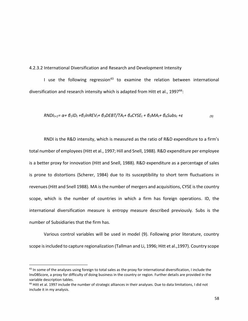
58
4.2.3.2 International Diversification and Research and Development Intensity
I use the following regression43 to examine the relation between international
diversification and research intensity which is adapted from Hitt et al., 199744:
RNDIt+1= α+ β1IDt +β2lnREVt+ β3DEBT/TAt+ β4CYSEt + β5MAt+ β6Subst +ε (9)
RNDI is the R&D intensity, which is measured as the ratio of R&D expenditure to a firm’s
total number of employees (Hitt et al., 1997; Hill and Snell, 1988). R&D expenditure per employee
is a better proxy for innovation (Hitt and Snell, 1988). R&D expenditure as a percentage of sales
is prone to distortions (Scherer, 1984) due to its susceptibility to short term fluctuations in
revenues (Hitt and Snell 1988). MA is the number of mergers and acquisitions, CYSE is the country
scope, which is the number of countries in which a firm has foreign operations. ID, the
international diversification measure is entropy measure described previously. Subs is the
number of Subsidiaries that the firm has.
Various control variables will be used in model (9). Following prior literature, country
scope is included to capture regionalization (Tallman and Li, 1996; Hitt et al.,1997). Country scope
43 In some of the analyses using foreign to total sales as the proxy for international diversification, I include the InvDBScore, a proxy for difficulty of doing business in the country or region. Further details are provided in the variable description tables. 44 Hitt et al. 1997 include the number of strategic alliances in their analyses. Due to data limitations, I did not include it in my analysis.

59
is measured by the number of countries in which a firm has foreign operations. Two-digit sic
codes will be used to control for industry effects. Other control variables include size, capital
structure (debt structure).
Hypothesis 3 is non- directional. β1 captures the relation between the level of
international diversification and R&D intensity. A positive coefficient of β1 will provide support
for a positive relation between the degree of international diversification and R&D intensity.
Similarly, a negative coefficient of β1 predicts will provide evidence of a positive relation between
international diversification and R&D intensity.
4.2.3.3 The Degree of Uncertainty of Future Benefits from Investments
One of the measures commonly used to measure the degree of uncertainty is the
variations in future value (e.g., Kothari et al., 2002; Amir et al., 2007; Li, 2011). In examining the
impact of diversification on the degree of uncertainty attributed to investment in R&D
expenditures, I use the following models (adapted from Kothari et al., 2002; Amir et al., 2007;
Asdemir et al., 2012):
SD (FVt+1, t+5) = α+ β1ID t + β2RND + β3RNDt *ID + β4CAPEX t + β5ADEX t + β6FLEV t + β7MV t +
Errort+1, t+5 (10)
SD (FVt+1, t+5) is the standard deviation of future benefits. The proxies for FV are sales
revenue, earnings before depreciation, amortization, advertising and R&D, or operating cash
flows. Each measure of future value will be examined separately. RND is the current investment

60
in R&D deflated by lagged market value of equity. ID is the international diversification measure.
CAPEX is the current investments in fixed capital deflated by lagged market value of equity. ADEX
is the advertising expenditure deflated by market value of equity, and FLEV is financial leverage,
MV is the market value of equity. MV is measured as the natural logarithm of the product of
share price and common shares outstanding.
H4 predicts that international diversification is associated with decreases in uncertainty
of future benefits from R&D expenditures. The interaction coefficient β3 indicates whether the
link between R&D and uncertainty of future benefits is moderated by international
diversification. A negative β3 means that the impact of international diversification on
uncertainty of future benefits from R&D investment grows more negative (less positive) at higher
levels of international diversification (H4: β3<0).
61
CHAPTER 5. RESULTS
5.1 Cost Rigidity- Results of Hypothesis Tests
The sample includes all US manufacturing firms (NAICS 31-33) from the annual
fundamentals file from 1990 -2019. The sample is restricted to firms that are internationally
diversified. All financial variables are deflated to control for inflation. Observations with missing
current or lagged sales are deleted. In SG&A analyses I delete observations if SG&A costs exceed
current sales or prior year sales. This is consistent with prior literature (e.g., Anderson et. al.,2003;
Banker et al.,2014). Following prior literature (e.g., Banker et al. 2014), I discard observations
where COGS is greater than 50 percent of current or prior year sales amount in COGS analyses.
To reduce the effect of outliers, data is winsorized at 1 percent and 99 percent.
After adjustments, the final data for FSTS consists of 133,018 observations for SG&A
analyses, 144,285 observations for COGS analyses and 109,793 for employees. For the data using
ID4 and ID7 as the proxy for international diversification, there are 110,268 observations for
SG&A analyses, 119,240 observations for COGS analyses, and 88,788 for employees. Analyses
using ID4 and ID7 as proxies for international diversification are lower in each case due to more
variations and missing information in segment data available in the Compustat segment files.
Table 1 panel B presents descriptive statistics for the sample used in cost rigidity analyses.
The mean deflated sales revenue is $1,157.46 million, measured using the average 1982-1984
dollars. The median is $ 193.72 million. SG&A and COGS account for an average of 40.81 percent
and 60.49 percent of sales revenue respectively. The median SG&A cost is 27.80 percent of
revenue. The median cost of goods sold is 61.77% of sales revenue. The average (median) number
of employees per firm is 7,960(1,740). Using the ID4, the Hitt et al. (1997) measure, the
62
mean(median) international diversification level is 0.284(0.314). For ID7, mean (median) level of
international diversification is 0.280(0.313). ID4 and ID7 have similar characteristics. Differences
in the calculations arise from the number of regions in each case. The mean(median) of the
InvDBScore is 18.42(18.59). For this sample, the average number of foreign countries in which a
firm operates is 25.35. The median number of countries is 22.
In the following analyses, I follow the approach in Banker et al. (2014) in estimating the
relation between international diversification and cost rigidity. FSTS_dc is the combined effect
of FSTS, CYSE and InvDBScore. CYSE and InvDBScore are added to the model because FSTS is
limited as it only captures the ratio of foreign to total sales. The inclusion of country scope (CYSE)
adds a dimension of the reach and complexity of doing business in multiple countries.
InvDBScore captures the difficulty of doing business in the country. For each firm, InvDBScore is
calculated as 100 minus the firm’s average doing-business score. Doing-business-score is
published by the world bank, and it measures the ease of doing business in each country. The
score is the aggregation of scores from ten categories including starting a business, dealing with
construction permits, getting electricity, registering property, getting credit, protecting minority
investors, paying taxes, trading across borders, enforcing contracts and resolving insolvency.
These factors affect multinational’s ease of entering and doing business in each country or region.

63
Table 1: Cost Rigidity -Descriptive Statistics
Variable Mean Standard Deviation Median Q1 Q3
Sales(deflated) $1,157.46 $3,354.67 $193.72 $43.96 $770.92
SG&A expenses(deflated) $245.36 $772.71 $44.33 $14.37 $150.77
Ratio of SG&A to sales 40.81% 64.12% 27.80% 16.44% 42.87%
COGS (deflated) $691.64 $1,986.21 $111.48 $22.73 $460.86
Ratio of COGS to sales 60.49% 26.47% 61.77% 47.10% 73.59%
Number of Employees 7.96 18.30 1.74 0.37 6.78
ID4 0.284 0.088 0.314 0.246 0.352
ID7 0.280 0.091 0.313 0.240 0.352
FSTS 0.382 0.272 0.393 0.142 0.580
InvDBScore 18.417 7.135 18.590 13.660 23.348
CYSE 25.346 19.420 22.000 10.00 37.000
5.1.1 Firms with low to medium levels of international diversification
Table 2 presents the estimates for SG&A costs for firms with low to medium levels
of international diversification. For each of the three international diversification proxies,
column (a) presents results for the model without the ID measure. Therefore, for each
column (a), the slope on the log-change sales, βi,t, is equal to Average β1+ γ1controls i,t..
β1+Y1 Controls measures the average short-run change in costs in response to a one
percent change in sales, thus capturing the average degree of cost rigidity. In column (b),
the results with the ID measure are presented for each of the three ID proxies. β2 captures
the relation between international diversification and cost rigidity. It measures the effect
of ID on the slope βi,t. For all three column(a) results, the average estimate of the slope
β1+Y1 Controls is between 1 and 0. This means that costs adjust to changes in sales, but
less than proportionately. From the results, a one percent increase in sales leads to an
average increase of between 0.632 and 0.834 percent in SG&A costs.
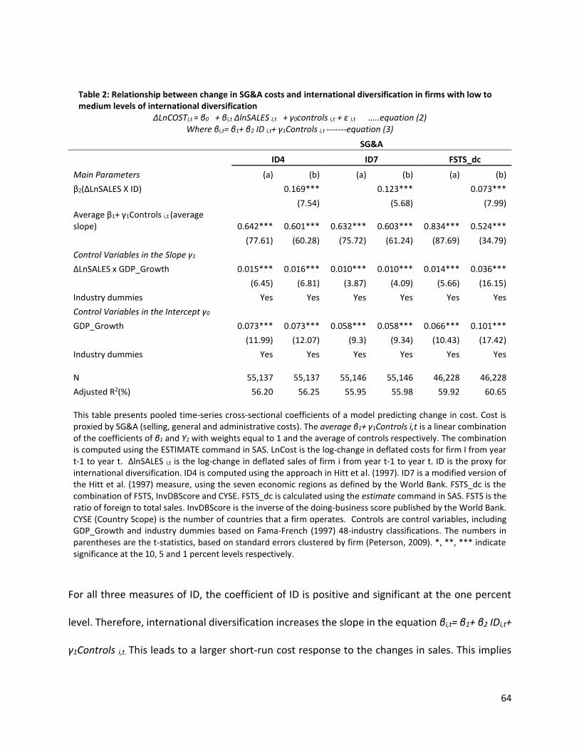
64
Table 2: Relationship between change in SG&A costs and international diversification in firms with low to medium levels of international diversification
ΔLnCOSTi,t = β0 + βi,t ΔlnSALES i,t + γ0controls i,t + ε i,t …..equation (2) Where βi,t= β1+ β2 ID i,t+ γ1Controls i,t -------equation (3)
SG&A
ID4 ID7 FSTS_dc
Main Parameters (a) (b) (a) (b) (a) (b)
β2(ΔLnSALES X ID) 0.169*** 0.123*** 0.073***
(7.54) (5.68) (7.99) Average β1+ γ1Controls i,t (average slope) 0.642*** 0.601*** 0.632*** 0.603*** 0.834*** 0.524***
(77.61) (60.28) (75.72) (61.24) (87.69) (34.79)
Control Variables in the Slope γ1
ΔLnSALES x GDP_Growth 0.015*** 0.016*** 0.010*** 0.010*** 0.014*** 0.036***
(6.45) (6.81) (3.87) (4.09) (5.66) (16.15)
Industry dummies Yes Yes Yes Yes Yes Yes
Control Variables in the Intercept γ0
GDP_Growth 0.073*** 0.073*** 0.058*** 0.058*** 0.066*** 0.101***
(11.99) (12.07) (9.3) (9.34) (10.43) (17.42)
Industry dummies Yes Yes Yes Yes Yes Yes
N
55,137
55,137
55,146
55,146
46,228
46,228
Adjusted R2(%) 56.20 56.25 55.95 55.98 59.92 60.65 This table presents pooled time-series cross-sectional coefficients of a model predicting change in cost. Cost is proxied by SG&A (selling, general and administrative costs). The average β1+ γ1Controls i,t is a linear combination of the coefficients of β1 and Y1 with weights equal to 1 and the average of controls respectively. The combination is computed using the ESTIMATE command in SAS. LnCost is the log-change in deflated costs for firm I from year t-1 to year t. ΔlnSALES i,t is the log-change in deflated sales of firm i from year t-1 to year t. ID is the proxy for international diversification. ID4 is computed using the approach in Hitt et al. (1997). ID7 is a modified version of the Hitt et al. (1997) measure, using the seven economic regions as defined by the World Bank. FSTS_dc is the combination of FSTS, InvDBScore and CYSE. FSTS_dc is calculated using the estimate command in SAS. FSTS is the ratio of foreign to total sales. InvDBScore is the inverse of the doing-business score published by the World Bank. CYSE (Country Scope) is the number of countries that a firm operates. Controls are control variables, including GDP_Growth and industry dummies based on Fama-French (1997) 48-industry classifications. The numbers in parentheses are the t-statistics, based on standard errors clustered by firm (Peterson, 2009). *, **, *** indicate significance at the 10, 5 and 1 percent levels respectively.
For all three measures of ID, the coefficient of ID is positive and significant at the one percent
level. Therefore, international diversification increases the slope in the equation βi,t= β1+ β2 IDi,t+
γ1Controls i,t. This leads to a larger short-run cost response to the changes in sales. This implies
65
that for these firms, an increase in international diversification, is associated with a less rigid
short-run cost structure. This finding is consistent with hypothesis 1a. The effect from ID4 is
greater than that from ID7 and FSTS_dc. For all three ID measures, a change in sales is associated
with a higher slope βi,t in the regression of log-change in SG&A costs on log-change in sales,
indicating a negative relationship between international diversification and cost rigidity.
Table 3 presents the results of the examination of the relation between international
diversification and rigidity of the changes in the cost of goods sold in response to changes in sales.
The sample consists of firms with low to medium levels of international diversification. For all
three analyses, the average slope in column (a) is positive and significantly different from 0 and
1. For analyses using ID4, ID7 and FSTS_dc, the average cost rigidity is 0.895, 0.888 and 0.927
respectively. From the first column, a 1 percent increase in sales, increases COGS by 0.895
percent.
The estimate of β2 is positive and significant at the 1 percent level when ID4 and ID7 are
the proxies for international diversification. This implies that international diversification
increases the slope βi,t= β1+ β2 IDi,t+ γ1Controls i,t. resulting in a larger short-run cost response to
the same change in sales. These results indicate that for firms with low to medium levels of
international diversification, an increase in international diversification is associated with lower
rigidity in the short run. This supports hypothesis 1a (H1a: β2 >0). Contrary to predictions, the
coefficient of FSTS_dc is negative and significant.

66
Table 3: Relationship between change in COGS costs and international diversification in firms with low to
medium levels of international diversification ΔLnCOSTi,t = β0 + βi,t ΔlnSALES i,t + γ0controls i,t + ε i,t …..equation (2)
Where βi,t= β1+ β2 IDi,t+ γ1Controls i,t -------equation (3)
COGS
ID4 ID7 FSTS_dc
Main Parameters (a) (b) (a) (b) (a) (b)
β2(ΔLnSALES X ID) 0.098*** 0.090*** -0.051***
(5.43) (5.23) (- 3.43) Average β1+ γ1controls i,t (average slope) 0.895*** 0.871*** 0.888*** 0.867*** 0.927*** 0.880***
(127.07) (104.91) (125.30) (106.08) (139.49) (87.81)
Control Variables in the Slope γ1
ΔLnSALES x GDP_Growth 0.027*** 0.027*** 0.026*** 0.027*** 0.027*** 0.025***
(13.40) (13.57) (13.11) (13.25) (12.77) (11.87)
Industry dummies Yes Yes Yes Yes Yes Yes
Control Variables in the Intercept γ0
GDP_Growth 0.047*** 0.047 0.045*** 0.045*** 0.071*** 0.064***
(9.38) (9.37) (9.10) (9.09) (13.56) (12.16)
Industry dummies Yes Yes Yes Yes Yes Yes
N 59,595 59,595 59,633 59,633 49,735 49,735
Adjusted R2(%) 72.40 72.42 72.44 72.45 75.52 75.64 This table presents pooled time-series cross-sectional coefficients of a model predicting change in cost. Cost is proxied by COGS (cost of goods sold). The average β1+ γ1Controls i,t is a linear combination of the coefficients of β1 and Y1 with weights equal to 1 and the average of controls respectively. The combination is computed using the ESTIMATE command in SAS. LnCost is the log-change in deflated costs for firm I from year t-1 to year t. ΔlnSALES i,t is the log-change in deflated sales of firm i from year t-1 to year t. ID is the proxy for international diversification. ID4 is computed using the approach in Hitt et al. (1997). ID7 is a modified version of the Hitt et al. (1997) measure, using the seven economic regions as defined by the World Bank. FSTS_dc is the combination of FSTS, InvDBScore and CYSE. FSTS_dc is calculated using the estimate command in SAS. FSTS is the ratio of foreign to total sales. InvDBScore is the inverse of the doing-business score published by the World Bank. CYSE (Country Scope) is the number of countries that a firm operates. Controls are control variables, including GDP_Growth and industry dummies based on Fama-French (1997) 48-industry classifications. The numbers in parentheses are the t-statistics, based on standard errors clustered by firm (Peterson, 2009). *, **, *** indicate significance at the 10, 5 and 1 percent levels respectively.
The results in table 4 are for analysis for the number of employees using the subsample
of firms with low to medium levels of international diversification. The average slope in column
(a) is positive and significant in all three analyses. A one percent increase in sales is associated

67
Table 4: Relationship between change in COGS costs and international diversification in firms with low to medium levels of international diversification
ΔLnCOSTi,t = β0 + βi,t ΔlnSALES i,t + γ0controls i,t + ε i,t …..equation (2) Where βi,t= β1+ β2 IDi,t+ γ1Controls i,t -------equation (3)
Employees
ID4 ID7 FSTS_dc
Main Parameters (a) (b) (a) (b) (a) (b)
β2(ΔLnSALES X ID) 0.143*** 0.126*** 0.007
(4.29) (3.95) (0.21) Average β1+ γ1Controls i,t (average slope) 0.545*** 0.510*** 0.541*** 0.511*** 0.455*** 0.410***
(44.10) (34.47) (43.77) (35.24) (34.77) (21.35)
Control Variables in the Slope γ1
ΔLnSALES x GDP_Growth 0.084*** 0.084*** 0.084*** 0.084*** 0.024*** 0.024***
(24.24) (24.36) (24.23) (24.36) (5.85) (5.85)
Industry dummies Yes Yes Yes Yes Yes Yes
Control Variables in the Intercept γ0
GDP_Growth 0.219*** 0.219*** 0.218*** 0.218*** 0.077*** 0.077***
(26.06) (26.06) (25.91) (25.92) (7.80) (7.79)
Industry dummies Yes Yes Yes Yes Yes Yes
N 44,389 44,389 44,362 44,362 36,645 36,645
Adjusted R2(%) 50.17 50.19 49.75 49.75 50.90 50.94 This table presents pooled time-series cross-sectional coefficients of a model predicting change in cost. Cost is proxied by the number of employees. The average β1+ γ1Controls i,t is a linear combination of the coefficients of β1 and Y1 with weights equal to 1 and the average of controls respectively. The combination is computed using the ESTIMATE command in SAS. LnCost is the log-change in deflated costs for firm I from year t-1 to year t. ΔlnSALES i,t is the log-change in deflated sales of firm i from year t-1 to year t. ID is the proxy for international diversification. ID4 is computed using the approach in Hitt et al. (1997). ID7 is a modified version of the Hitt et al. (1997) measure, using the seven economic regions as defined by the World Bank. FSTS_dc is the combination of FSTS, InvDBScore and CYSE. FSTS_dc is calculated using the estimate command in SAS. FSTS is the ratio of foreign to total sales. InvDBScore is the inverse of the doing-business score published by the World Bank. CYSE (Country Scope) is the number of countries that a firm operates. Controls are control variables, including GDP Growth and industry dummies based on Fama-French (1997) 48 industry classifications. The numbers in parentheses are the t-statistics, based on standard errors clustered by firm (Peterson, 2009). *, **, *** indicate significance at the 10, 5 and 1 percent levels respectively.
with an increase of 0.545(0.455) percent change in the number of employees when ID4(FSTS_dc)
is the measure of international diversification.
In column (b), the coefficients of ID4 and ID7 are both positive and significant at the 1
percent level. This is consistent with the predictions. The positive and significant coefficients
68
mean that, for firms with low to medium levels of international diversification, an increase in
international is associated with an increase in the slope in the equation βi,t= β1+ β2 IDi,t+ γ1Controls
i,t. This results in a larger short-run cost response to the changes in sales. This implies that for
these firms, an increase in international diversification, is associated with a less rigid short-run
cost structure. These results support hypothesis 1a. That is the prediction that at low to medium
levels international diversification, an increase in international diversification is associated with
a less rigid cost structure. Though the coefficient of FSTS_dc is positive as expected, it is
insignificant. Therefore, the FSTS_dc result fails to lend support to hypothesis 1a.
5.1.2 Firms with higher levels of international diversification
This section presents the results for firms with higher levels of international
diversification. The firms included in the sample are those that have an international
diversification measure (ID4, ID7 and FSTS) that is greater than the median. Table 5 presents the
estimates for SG&A costs. In column (a) the slope on the log-change sales, βi, t is equal to β1+γ1
Controls and ID is set to zero. β1+γ1 Controls measures the average short-run change in costs to
a one percent change in sales, thus capturing the average degree of cost rigidity. Column (b)
includes the ID measure. The results are presented for each of the three international
diversification proxies. β2 captures the relation between international diversification and cost
rigidity. It measures the effect of ID on the slope βi, t.
From the results, the average estimate of the slope β1+ γ1controls i,t is 0.796, 0.768 and
0.650 for regressions using ID4, ID7 and FSTS_dc respectively. For all three, the coefficients are
significant at the one percent level. This means that costs adjust to changes in sales, but less than
69
proportionately. A one percent increase in sales leads to an average increase of 0.796(0.768)
percent in SG&A costs when ID4(ID7) is the international diversification proxy.
Turning to column (b) results, the coefficient of ID is negative and significant at the one
percent level for all the three proxies for international diversification. Therefore, international
diversification decreases the slope in the equation βi,t= β1+ β2 IDi,t+ γ1Controls i,t.. This results in a
smaller short-run cost response to the changes in sales. For ID4, ID7 and FSTS_dc, a higher log-
changes in sales is associated with a smaller slope βi,t. in the regression of log-change in SG&A
costs on log-change in sales, indicating a positive relationship between international
diversification and cost rigidity. This implies that for these firms, an increase in international
diversification, is associated with a more rigid short-run cost structure. This finding is consistent
with hypothesis 1b. Hypothesis 1b predicts that at higher levels of international diversification,
there is positive association between international diversification and cost rigidity.
The results for cost of goods sold are presented in table 6. From the results, the
coefficients of the average estimate of the slope β1+ γ1controls i,t..are significant at the one
percent level in column (a). The results indicate that a one percent increase in sales is
accompanied by an increase in COGS by 0.892(0.916) percent when the ID proxy is ID4 (FSTS_dc).
This change is significantly different from zero and one. This indicates that COGS respond to a
change in sales but not proportionately. The change is significantly different from zero and one.
This finding is consistent with prior findings (e.g., Banker et al.,2014). The coefficients of ID4 and
ID7 are positive and insignificant. Hypothesis 1b, predicts that for firms with high levels of
international diversification, increases in international diversification leads to greater cost
rigidity. A negative coefficient of β2 would offer support for this prediction.
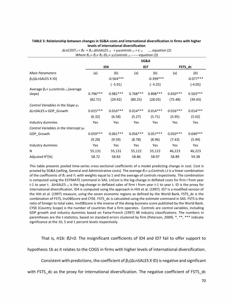
70
TABLE 5: Relationship between changes in SG&A costs and international diversification in firms with higher levels of international diversification
ΔLnCOSTi,t = β0 + βi,t ΔlnSALES i,t + γ0controls i,t + ε i,t …..equation (2) Where βi,t= β1+ β2 IDi,t+ γ1Controls i,t -------equation (3)
SG&A
ID4 ID7 FSTS_dc
Main Parameters (a) (b) (a) (b) (a) (b)
β2(ΔLnSALES X ID) -0.564*** -0.399*** -0.077***
( -5.91) (- 4.25) (-4.05) Average β1+ γ1controls i,t (average slope) 0.796*** 0.981*** 0.768*** 0.898*** 0.650*** 0.503***
(82.71) (29.92) (80.25) (28.03) (75.48) (39.43)
Control Variables in the Slope γ1
ΔLnSALES x GDP_Growth 0.015*** 0.016*** 0.014*** 0.014*** 0.016*** 0.014***
(6.32) (6.58) (5.27) (5.71) (5.95) (5.02)
Industry dummies Yes Yes Yes Yes Yes Yes
Control Variables in the Intercept γ0
GDP_Growth 0.059*** 0.061*** 0.056*** 0.057*** 0.050*** 0.040***
(9.28) (9.59) (8.78) (8.96) (7.43) (5.94)
Industry dummies Yes Yes Yes Yes Yes Yes
N 55,131 55,131 55,122 55,122 46,223 46,223
Adjusted R2(%) 58.72 58.83 58.86 58.97 58.89 59.38 This table presents pooled time-series cross-sectional coefficients of a model predicting change in cost. Cost is proxied by SG&A (selling, General and Administrative costs). The average β1+ γ1Controls i,t is a linear combination of the coefficients of β1 and Y1 with weights equal to 1 and the average of controls respectively. The combination is computed using the ESTIMATE command in SAS. LnCost is the log-change in deflated costs for firm I from year t-1 to year t. ΔlnSALES i,t is the log-change in deflated sales of firm i from year t-1 to year t. ID is the proxy for international diversification. ID4 is computed using the approach in Hitt et al. (1997). ID7 is a modified version of the Hitt et al. (1997) measure, using the seven economic regions as defined by the World Bank. FSTS_dc is the combination of FSTS, InvDBScore and CYSE. FSTS_dc is calculated using the estimate command in SAS. FSTS is the ratio of foreign to total sales. InvDBScore is the inverse of the doing-business score published by the World Bank. CYSE (Country Scope) is the number of countries that a firm operates. Controls are control variables, including GDP growth and industry dummies based on Fama-French (1997) 48 industry classifications. The numbers in parentheses are the t-statistics, based on standard errors clustered by firm (Peterson, 2009). *, **, *** indicate significance at the 10, 5 and 1 percent levels respectively.
That is, H1b: β2<0. The insignificant coefficients of ID4 and ID7 fail to offer support to
hypothesis 1b as it relates to the COGS in firms with higher levels of international diversification.
Consistent with predictions, the coefficient of β2(ΔLnSALES X ID) is negative and significant
with FSTS_dc as the proxy for international diversification. The negative coefficient of FSTS_dc
71
lends support to hypothesis 2. The negative coefficient of β2 means that international
diversification reduces the slope of βi,t= β1+ β2 IDi,t+ γ1Controls i,t , resulting in a smaller COGS
response for the same change in sales. Therefore, for firms with higher levels of international
diversification, ID is associated with a more rigid short-run cost structure as it relates to COGS.
The results examining the rigidity in the number of employees in response to changes in
sales are presented in table 7. The coefficients of the average β1+ γ1controls i,t are positive and
significant at the 1 percent level. On average, a one percent increase in sales, is associated with
an increase in the number of employees increases by 0.273 percent (0.271 percent) in the
analyses using ID4(ID7) as the international diversification measure. For FSTS_dc, the average
change in the number of employees in response to a 1 percent change in sales is 0.328 percent.
All three coefficients are significant at the 1 percent level.
In the column(b) results, the coefficients of ID4 and ID7 are negative and significant. The
coefficient of ID4 is -0.50 with a t-value of -2.97. Similarly, the coefficient of ID7 is -0.37 and the
t-value is 2.21. Hypothesis 1b, predicts that for firms with higher levels of diversification,
international diversification is positively associated with cost rigidity.
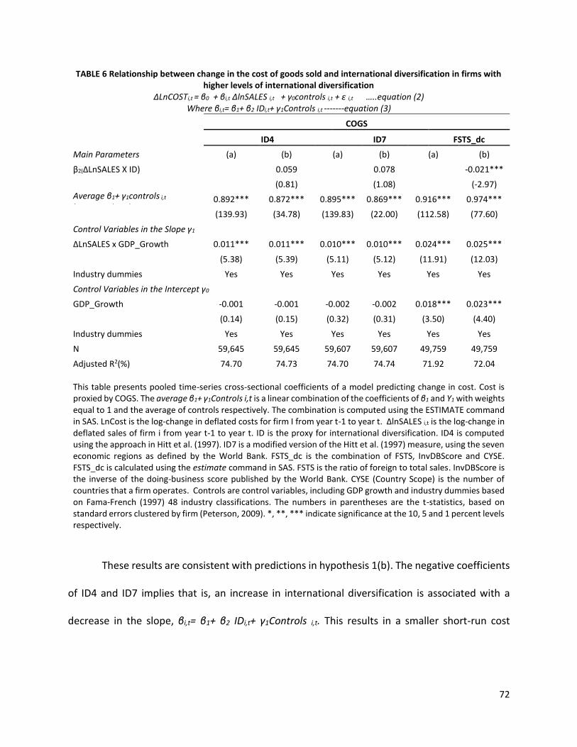
72
TABLE 6 Relationship between change in the cost of goods sold and international diversification in firms with higher levels of international diversification
ΔLnCOSTi,t = β0 + βi,t ΔlnSALES i,t + γ0controls i,t + ε i,t …..equation (2) Where βi,t= β1+ β2 IDi,t+ γ1Controls i,t -------equation (3)
COGS
ID4 ID7 FSTS_dc
Main Parameters (a) (b) (a) (b) (a) (b)
β2(ΔLnSALES X ID) 0.059 0.078 -0.021***
(0.81) (1.08) (-2.97) Average β1+ γ1controls i,t (average slope)
0.892*** 0.872*** 0.895*** 0.869*** 0.916*** 0.974***
(139.93) (34.78) (139.83) (22.00) (112.58) (77.60)
Control Variables in the Slope γ1
ΔLnSALES x GDP_Growth 0.011*** 0.011*** 0.010*** 0.010*** 0.024*** 0.025***
(5.38) (5.39) (5.11) (5.12) (11.91) (12.03)
Industry dummies Yes Yes Yes Yes Yes Yes
Control Variables in the Intercept γ0
GDP_Growth -0.001 -0.001 -0.002 -0.002 0.018*** 0.023***
(0.14) (0.15) (0.32) (0.31) (3.50) (4.40)
Industry dummies Yes Yes Yes Yes Yes Yes
N 59,645 59,645 59,607 59,607 49,759 49,759
Adjusted R2(%) 74.70 74.73 74.70 74.74 71.92 72.04 This table presents pooled time-series cross-sectional coefficients of a model predicting change in cost. Cost is proxied by COGS. The average β1+ γ1Controls i,t is a linear combination of the coefficients of β1 and Y1 with weights equal to 1 and the average of controls respectively. The combination is computed using the ESTIMATE command in SAS. LnCost is the log-change in deflated costs for firm I from year t-1 to year t. ΔlnSALES i,t is the log-change in deflated sales of firm i from year t-1 to year t. ID is the proxy for international diversification. ID4 is computed using the approach in Hitt et al. (1997). ID7 is a modified version of the Hitt et al. (1997) measure, using the seven economic regions as defined by the World Bank. FSTS_dc is the combination of FSTS, InvDBScore and CYSE. FSTS_dc is calculated using the estimate command in SAS. FSTS is the ratio of foreign to total sales. InvDBScore is the inverse of the doing-business score published by the World Bank. CYSE (Country Scope) is the number of countries that a firm operates. Controls are control variables, including GDP growth and industry dummies based on Fama-French (1997) 48 industry classifications. The numbers in parentheses are the t-statistics, based on standard errors clustered by firm (Peterson, 2009). *, **, *** indicate significance at the 10, 5 and 1 percent levels respectively.
These results are consistent with predictions in hypothesis 1(b). The negative coefficients
of ID4 and ID7 implies that is, an increase in international diversification is associated with a
decrease in the slope, βi,t= β1+ β2 IDi,t+ γ1Controls i,t. This results in a smaller short-run cost

73
response for the same change in sales. Therefore, increases in international diversification is
associated with a more rigid short-run cost structure. This supports hypothesis 1b.
Contrary to predictions, the coefficient of β2(ΔLnSALES X ID) is positive when FSTS_dc is
the proxy for international diversification. This result is inconsistent with results for ID4 and ID7,
the other two proxies of international diversification. As noted previously, this inconsistency may
be attributable to the fact that FSTS together with CYSE and InvDBScore captures different
aspects of international diversification. Hitt et al., (1997) argue for that their measure (ID4 in this
case), captures the breath and width of international diversification, by including both the
proportion of sales and the weight of each global market region in the calculation. ID7 follows
similar criteria with redefined regions. The control variables in the regression using FSTS_dc as
the proxy for international diversification are similar in direction to the ones in the regressions
using ID4 and ID7.
5.1.3 Additional analyses
In the main analyses, results from using FSTS_dc as the proxy for international
diversification are partially consistent with the results for ID4 and ID7. Part of the reason could
be from the inclusion of a proxy for the degree of challenges faced by multinationals in the foreign
markets (InvDBScore) and country scope (CYSE) in the FSTS_dc measure. To explore this, I rerun
FSTS analyses without including InvDBScore and CYSE.
Appendix 3 presents the results for SGA, COGS and Employees for firms with low to
medium levels of international diversification. In the SG&A analyses, the coefficient of FSTS is
consistent with the coefficient of FSTS_dc. It is positive and significant at the 1 percent level.

74
TABLE 7: Relationship between change in the number of employees and international diversification in firms with higher levels of international diversification
ΔLnCOSTi,t = β0 + βi,t ΔlnSALES i,t + γ0controls i,t + ε i,t …..equation (2) Where βi,t= β1+ β2 IDi,t+ γ1Controls i,t -------equation (3)
Employees
ID4 ID7 FSTS_dc
Main Parameters (a) (b) (a) (b) (a) (b)
β2(ΔLnSALES X ID) -0.500*** -0.370** 0.088***
(-2.97) (-2.21) (6.28) Average β1+ γ1controls i,t (average slope) 0.273*** 0.448*** 0.271*** 0.401*** 0.328*** 0.239***
(22.74) (7.47) (22.51) (6.71) (22.70) (10.35)
Control Variables in the Slope γ1
ΔLnSALES x GDP_Growth 0.046*** 0.046*** 0.046*** 0.045*** 0.048*** 0.051***
(15.72) (15.67) (15.48) (15.42) (15.39) (16.16)
Industry dummies Yes Yes Yes Yes Yes Yes
Control Variables in the Intercept γ0
GDP_Growth 0.141*** 0.141*** 0.140*** 0.139*** 0.169*** 0.180***
(17.59) (17.54) (17.37) (17.33) (19.62) (20.93)
Industry dummies Yes Yes Yes Yes Yes Yes
N 44,399 44,399 44,426
44,426
36,987
36,987
Adjusted R2(%) 48.68 48.69 48.76 48.76 44.13 48.49 This table presents pooled time-series cross-sectional coefficients of a model predicting change in cost. Cost is proxied by the number of employees. The average β1+ γ1Controls i,t is a linear combination of the coefficients of β1 and Y1 with weights equal to 1 and the average of controls respectively. The combination is computed using the ESTIMATE command in SAS. LnCost is the log-change in deflated costs for firm I from year t-1 to year t. ΔlnSALES i,t is the log-change in deflated sales of firm i from year t-1 to year t. ID is the proxy for international diversification. ID4 is computed using the approach in Hitt et al. (1997). ID7 is a modified version of the Hitt et al. (1997) measure, using the seven economic regions as defined by the World Bank. FSTS_dc is the combination of FSTS, InvDBScore and CYSE. FSTS_dc is calculated using the estimate command in SAS. FSTS is the ratio of foreign to total sales. InvDBScore is the inverse of the doing-business score published by the World Bank. CYSE (Country Scope) is the number of countries that a firm operates. Controls are control variables, including GDP growth and industry dummies based on Fama-French (1997) 48 industry classifications. The numbers in parentheses are the t-statistics, based on standard errors clustered by firm (Peterson, 2009). *, **, *** indicate significance at the 10, 5 and 1 percent levels respectively.
This result is similar in direction to those for ID4 and ID7 in the main analyses. For COGS,
the coefficient of FSTS is positive and significant at the 1 percent level. This is consistent to the
predictions and lends support to hypothesis 1a. In earlier analyses, the inclusion of InvDBScore
and CYSE resulted in a coefficient that is negative and contrary to predictions. For the regression

75
using the number of employees, the coefficient of FSTS is positive and insignificant. This is
consistent with the coefficient FSTS_dc in the main analysis. On the overall, the results from the
main analysis and the latter tests support hypothesis 1a. There is support for the prediction that
for firms with low to medium levels of international diversification, ID is associated with
decreases in cost rigidity.
Appendix 4 presents the results for SG&A, COGS, and employees for firms with higher
levels of international diversification. With the exclusion of InvDBScore and CYSE, the coefficient
of FSTS in the SG&A analyses is positive and significant at the 1 percent level. This conflicts with
the results in the main analyses for ID4, ID7 and FSTS_dc. In the main analyses, FSTS_dc is
negative and consistent with the predictions. For COGS, the coefficient of FSTS is positive and
significant at the 1 percent level. This is inconsistent with the predictions and does not lend
support for hypothesis 1a. This result is opposite to earlier findings for FSTS_dc. However, it is
notable that in this case the, the exclusion of InvDBScore and CYSE yielded results that are
consistent in direction with those of ID4 and ID7 in the main analyses. That is ID4, ID7 and FSTS
are all positive in the regressions for changes in COGS. However, ID4 and ID7 coefficients are
insignificant.
For the regression using the number of employees, the coefficient of FSTS is positive and
significant at the 1 percent level. This is consistent with the coefficient FSTS_dc in the main
analysis. Therefore, in the sample of firms with higher levels of international diversification,
results for both FSTS_dc and FSTS do not support hypothesis 1b as it pertains to the changes in
the number of employees.
76
5.2 Investment Efficiency - Results of Hypothesis Tests
5.2.1 Sample and descriptive statistics
The sample used in the investment efficiency analyses, is presented in table 8. The sample
consists of manufacturing firms with non-missing data on the variables used in the regressions.
Table 8 Panel C provides the variable definitions. After deleting observations with missing data,
the final sample includes 66,663 firm-year observations for regressions using FSTS (ratio of
foreign sales to total sales) as the international diversification measure and 54,325 and (54,337
firm-observations for analyses using ID4 and ID745 respectively, to proxy international
diversification. Financial information data is from Compustat, analyst data is from I/B/E/S and
governance data is from Gompers et al. (2003). Continuous variables are winsorized at the 1%
and 99% levels.
Panel A of table 8 presents descriptive statistics for the variables used in the investment
efficiency analyses. The mean(median) investment is 10.4% (7.8%) of prior year’s assets. The
mean(median) ID4 is 0.278(0.297) respectively. The mean(median) ID7 is 0.275 (0.295). Panel B
of table 8, presents the correlations among the variables. ID4 and ID7 are significantly correlated
with a rate of 0.97. FSTS has a lower correlation with both ID4 and ID7. The correlation rate is
significant at 0.20 and 0.19 respectively. ID4 and ID7 capture both the breadth and the width of
firms’ international diversification activities. FSTS captures only the weight of foreign sales
45 ID4 and ID7 are constructed using the Hitt et al. (1997) ID4 is based on the four regions used in Hitt et al. (1997). ID7 is based on the seven-region classification by the World Bank. The seven regions are East Asia and Pacific, Europe and Central Asia, Latin America and the Caribbean, Middle East and North Africa, North America, South Asia, and Sub-Saharan Africa. Appendix 1 provides further detail and illustration on the calculation of ID4 (Hitt et al.,1997) international diversification measure.
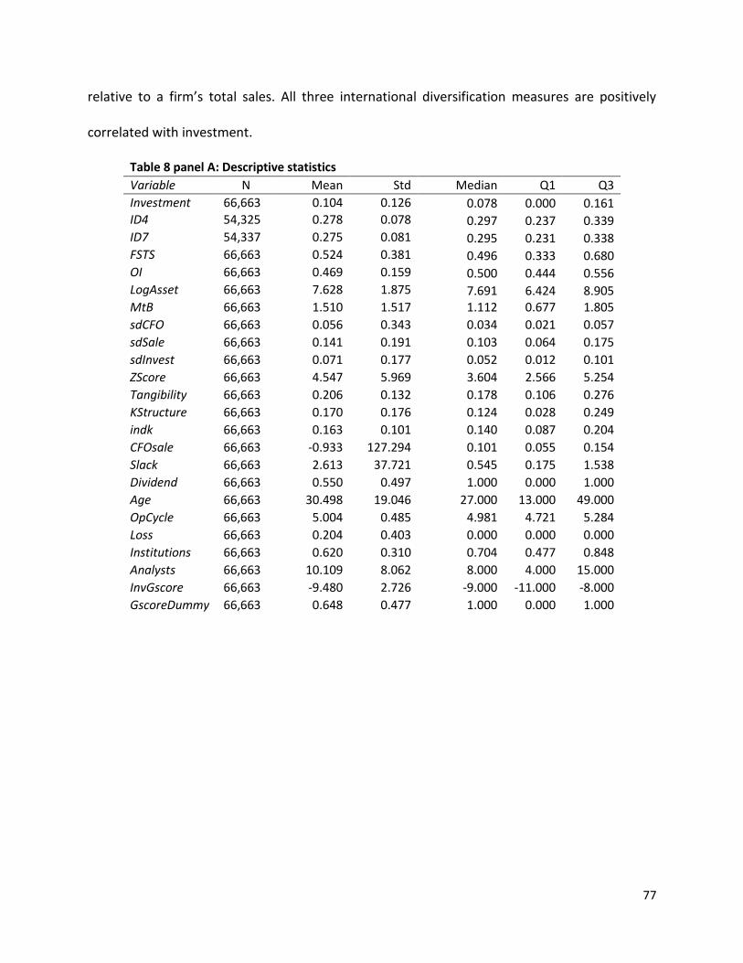
77
relative to a firm’s total sales. All three international diversification measures are positively
correlated with investment.
Table 8 panel A: Descriptive statistics
Variable N Mean Std Median Q1 Quartile
Q3
Investment 66,663 0.104 0.126 0.078 0.000 0.161 ID4 54,325 0.278 0.078 0.297 0.237 0.339 ID7 54,337 0.275 0.081 0.295 0.231 0.338 FSTS 66,663 0.524 0.381 0.496 0.333 0.680 OI 66,663 0.469 0.159 0.500 0.444 0.556 LogAsset 66,663 7.628 1.875 7.691 6.424 8.905 MtB 66,663 1.510 1.517 1.112 0.677 1.805
sdCFO 66,663 0.056 0.343 0.034 0.021 0.057
sdSale 66,663 0.141 0.191 0.103 0.064 0.175
sdInvest 66,663 0.071 0.177 0.052 0.012 0.101
ZScore 66,663 4.547 5.969 3.604 2.566 5.254
Tangibility 66,663 0.206 0.132 0.178 0.106 0.276
KStructure 66,663 0.170 0.176 0.124 0.028 0.249
indk 66,663 0.163 0.101 0.140 0.087 0.204
CFOsale 66,663 -0.933 127.294 0.101 0.055 0.154
Slack 66,663 2.613 37.721 0.545 0.175 1.538
Dividend 66,663 0.550 0.497 1.000 0.000 1.000
Age 66,663 30.498 19.046 27.000 13.000 49.000
OpCycle 66,663 5.004 0.485 4.981 4.721 5.284
Loss 66,663 0.204 0.403 0.000 0.000 0.000
Institutions 66,663 0.620 0.310 0.704 0.477 0.848
Analysts 66,663 10.109 8.062 8.000 4.000 15.000
InvGscore 66,663 -9.480 2.726 -9.000 -11.000 -8.000
GscoreDummy 66,663 0.648 0.477 1.000 0.000 1.000

78
Va
riab
leIn
ve
stm
en
tID
4ID
7F
ST
SO
ILo
gA
sse
tM
tBsd
CF
Osd
Sa
le
Inv
estm
en
t1
ID4
0.0
11
.00
ID7
0.0
10
.97
1.0
0
FS
TS
0.0
30
.20
0.1
91
.00
OI
-0.1
8-0
.06
-0.0
6-0
.12
1.0
0
Lo
gA
sse
t-0
.27
0.0
70
.07
0.0
70
.20
1.0
0
MtB
0.1
8-0
.02
-0.0
20
.00
-0.2
90
.03
1.0
0
sd
CF
O0
.07
-0.0
1-0
.01
0.0
0-0
.05
-0.0
90
.10
1.0
0
sd
Sa
le0
.08
-0.0
3-0
.03
-0.0
1-0
.06
-0.1
80
.04
0.8
01
.00
sd
Inv
est
0.1
6-0
.01
0.0
00
.01
-0.0
5-0
.13
0.1
00
.61
0.4
1
Zsco
re0
.08
-0.0
2-0
.01
-0.0
3-0
.37
-0.0
40
.62
0.0
10
.00
Ta
ng
ibility
-0.0
50
.01
0.0
0-0
.04
0.3
10
.12
-0.0
9-0
.04
-0.0
6
KS
tructu
re-0
.16
-0.0
3-0
.03
-0.0
60
.51
0.1
1-0
.47
-0.0
30
.01
Ind
k-0
.16
-0.0
4-0
.05
-0.1
00
.25
0.0
5-0
.30
-0.0
3-0
.03
CF
Osa
le-0
.06
-0.0
1-0
.01
-0.0
10
.00
0.0
2-0
.02
-0.0
2-0
.01
Sla
ck
0.0
7-0
.01
-0.0
10
.05
-0.2
5-0
.16
0.1
00
.10
0.1
1
Div
ide
nd
-0.2
3-0
.02
-0.0
3-0
.07
0.2
30
.43
-0.0
1-0
.06
-0.1
6
Ag
e-0
.25
0.0
10
.01
-0.0
50
.19
0.4
9-0
.03
-0.0
6-0
.16
Op
Cy
cle
0.1
10
.02
0.0
30
.06
-0.0
5-0
.17
0.1
30
.01
-0.0
8
LO
SS
0.1
3-0
.01
-0.0
10
.04
-0.0
7-0
.27
-0.1
50
.06
0.1
3
Institu
tion
s-0
.02
0.0
60
.06
0.0
2-0
.06
0.1
50
.03
-0.0
4-0
.10
An
aly
sts
-0.0
40
.02
0.0
20
.07
-0.0
30
.69
0.3
5-0
.04
-0.0
9
Gsco
reD
um
my
0.0
50
.00
-0.0
10
.04
-0.1
0-0
.15
-0.1
40
.02
0.0
6
Inv
Gsco
re0
.08
0.0
0-0
.01
0.0
5-0
.20
-0.0
10
.13
0.1
60
.09
Pa
ne
l B p
rese
nts
Pe
ars
on
co
rrela
tion
s. In
ve
stm
en
t is a
me
asu
re o
f tota
l inv
estm
en
t sca
led
by
lag
ge
d to
tal a
sse
ts. ID
is
the
inte
rna
tion
al d
ive
rsific
atio
n m
ea
su
re. ID
4 is
the
inte
rna
tion
al d
ive
rsific
atio
n c
on
stru
cte
d fo
llow
ing
Hitt e
t al. (1
99
7)
pro
ce
du
re, u
sin
g fo
ur e
co
no
mic
wo
rld re
gio
ns. ID
7 is
the
inte
rna
tion
al d
ive
rsific
atio
n c
on
stru
cte
d fo
llow
ing
Hitt e
t al.
(19
97
) pro
ce
du
re, u
sin
g s
ev
en
eco
no
mic
wo
rld re
gio
ns a
s id
en
tified
by
the
Wo
rld B
an
k in
its e
co
no
mic
rep
orts
.
Ta
ble
8: P
an
el B
: Pe
ars
on
Co
rrela
tion
s
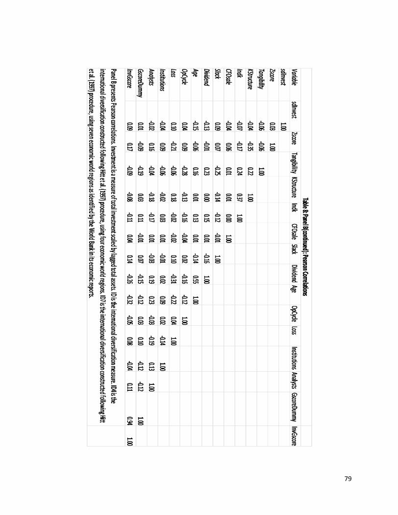
79
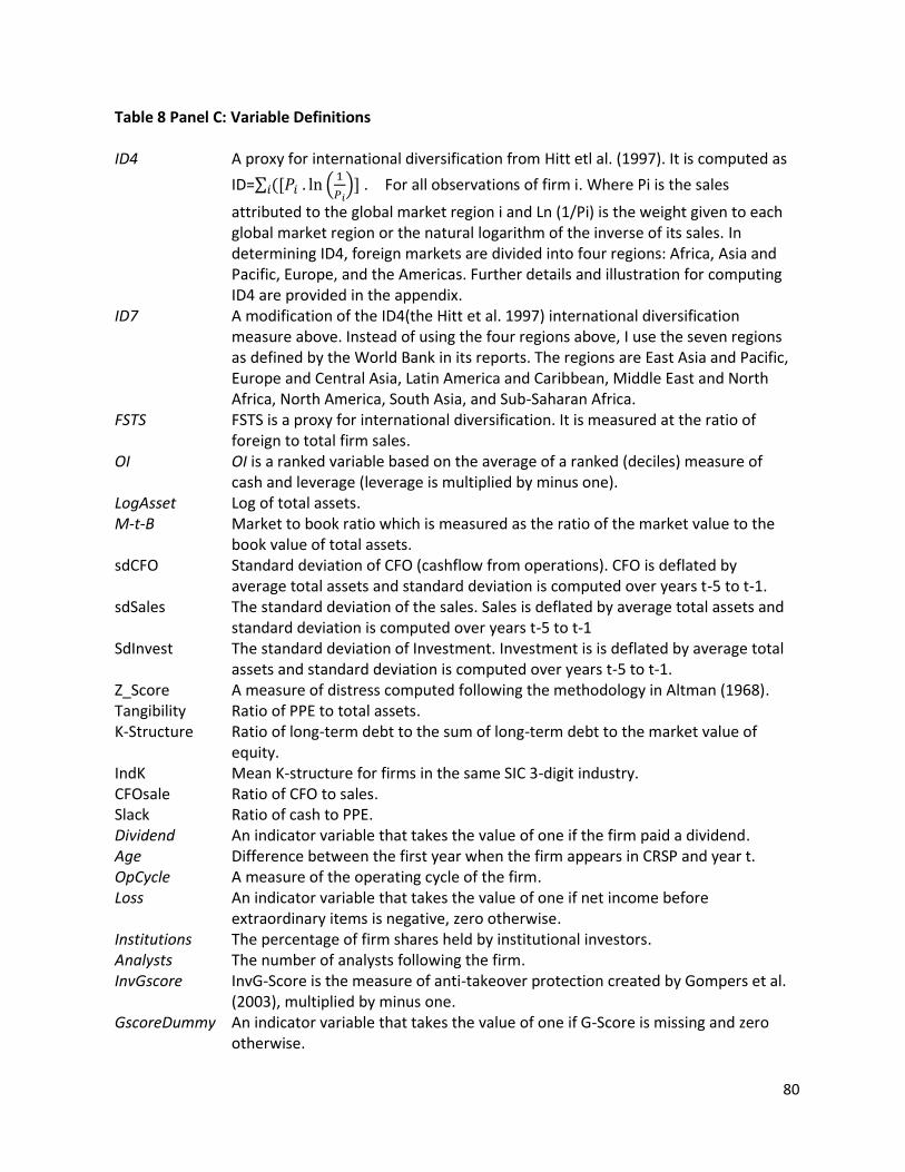
80
Table 8 Panel C: Variable Definitions
ID4 A proxy for international diversification from Hitt etl al. (1997). It is computed as
ID=∑ ([𝑃𝑖 . ln (1
𝑃𝑖)]𝑖 . For all observations of firm i. Where Pi is the sales
attributed to the global market region i and Ln (1/Pi) is the weight given to each global market region or the natural logarithm of the inverse of its sales. In determining ID4, foreign markets are divided into four regions: Africa, Asia and Pacific, Europe, and the Americas. Further details and illustration for computing ID4 are provided in the appendix.
ID7 A modification of the ID4(the Hitt et al. 1997) international diversification measure above. Instead of using the four regions above, I use the seven regions as defined by the World Bank in its reports. The regions are East Asia and Pacific, Europe and Central Asia, Latin America and Caribbean, Middle East and North Africa, North America, South Asia, and Sub-Saharan Africa.
FSTS FSTS is a proxy for international diversification. It is measured at the ratio of foreign to total firm sales.
OI OI is a ranked variable based on the average of a ranked (deciles) measure of cash and leverage (leverage is multiplied by minus one).
LogAsset Log of total assets. M-t-B Market to book ratio which is measured as the ratio of the market value to the
book value of total assets. sdCFO Standard deviation of CFO (cashflow from operations). CFO is deflated by
average total assets and standard deviation is computed over years t-5 to t-1. sdSales The standard deviation of the sales. Sales is deflated by average total assets and
standard deviation is computed over years t-5 to t-1 SdInvest The standard deviation of Investment. Investment is is deflated by average total
assets and standard deviation is computed over years t-5 to t-1. Z_Score A measure of distress computed following the methodology in Altman (1968). Tangibility Ratio of PPE to total assets. K-Structure Ratio of long-term debt to the sum of long-term debt to the market value of
equity. IndK Mean K-structure for firms in the same SIC 3-digit industry. CFOsale Ratio of CFO to sales. Slack Ratio of cash to PPE. Dividend An indicator variable that takes the value of one if the firm paid a dividend. Age Difference between the first year when the firm appears in CRSP and year t. OpCycle A measure of the operating cycle of the firm. Loss An indicator variable that takes the value of one if net income before
extraordinary items is negative, zero otherwise. Institutions The percentage of firm shares held by institutional investors. Analysts The number of analysts following the firm. InvGscore InvG-Score is the measure of anti-takeover protection created by Gompers et al.
(2003), multiplied by minus one. GscoreDummy An indicator variable that takes the value of one if G-Score is missing and zero
otherwise.
81
5.2.2 Conditional relation between international diversification and investment
5.2.2.1 Conditional tests: Firms with low to medium levels of international diversification
In these analyses, I use OI46 an aggregated measure of cash balance and leverage to
classify firms by the likelihood that they will over or underinvest. Results of running equation
(6) on the subsample of firms with low to medium levels of international diversification is
reported in table 9. That is, table 9 reports the results for test of hypothesis 2a and 2b which
focus on firms with low to medium levels of international diversification. I find weak evidence
that international diversification is positively associated with firms among firms with higher
likelihood of underinvesting. The coefficient of ID4 is significant with a t-statistic of 1.78.
Increasing ID4 by one standard deviation, increases investment by approximately 0.39%. This
lends support for H2b. Both ID7 and FSTS are not significant.
For the interaction between international diversification and over-investment, the
estimated coefficients are negative and significant for all three international diversification
measures. The t-statistics range from -2.32 for ID7 to -3.2 for FSTS. The overall effect of
international diversification on investment is measured by the sum of the coefficient of ID
and that of the interaction of ID and OI. From the results, the sum of the interactions is
negative and significant at the one percent level in all three analyses. This offers support to
hypothesis 2a.
46 OI is described in detail in section 4.2.3. To determine the measure, firms are ranked into deciles based on
cash balance and leverage. Leverage is multiplied by minus one, such that the measure is increasing with the likelihood for over-investment. I then create a combined measure (OI) using the average of the average of the two measures. Aggregation of the two measures reduces measurement error in the individual variables (Biddle et al.,2009).

82
TABLE 9: Conditional Relation between Investment and International Diversification Firms with low to medium Levels of international Diversification
Investment i, t+1 = α+ β1IDi,t+ β2IDi,t *OIi,t+1+ β3OIi,t+1 + ∑ 𝛾𝑗Control, j,j,t + εi,t+1 (6)
International diversification proxy
ID4 ID7 FSTS
Variable Parameter
Estimate (t-value) Parameter
Estimate (t-value)
Parameter Estimate (t-
value)
ID 0.050* 0.029 0.004
(1.78) (1.08) (0.15)
ID* OI -0.174*** -0.121** -0.147***
(-3.15) (-2.32) (-3.20)
β1+β2 -0.124*** -0.092*** -0.054***
(-3.93) (-3.08) (-2.89)
CYSE 0.000
(-0.33)
InvDBScore 0.003***
(13.00) Governance Variables
Institutions 0.036*** 0.034*** 0.000
(3.6) (3.49) (0.27)
Analysts -0.001*** -0.001*** -0.001
(-4.52) (-4.39) (0.18)
InvGscore -0.005*** -0.006*** 0.003**
(-3.67) (-4.18) (-2.00)
GscoreDummy 0.000 0.000 0.187
(-0.14) (-0.28) (-0.54)
Institution* OI -0.093*** -0.090*** 0.010
(-5.27) (-5.15) (-1.24)
Analysts* OI 0.005*** 0.005*** -0.092***
(8.38) (8.05) (4.34)
InvGscore* OI 0.004* 0.004* 0.000***
(1.65) (1.75) (4.51)
Control Variables
OI 0.151*** 0.142*** 0.095***
(4.93) (4.68) (5.84)
LogAsset -0.006** -0.006** -0.015***
(-2.53) (-2.23) (4.32) This table presents pooled time-series cross-sectional regression coefficients of a model predicting Investment. Investment is a measure of total investment scaled by lagged total assets. ID is the international diversification measure. ID4 is the international diversification constructed following Hitt et al. (1997) procedure, using four economic world regions. ID7 is the international diversification constructed following Hitt et al. (1997) procedure, using seven economic world regions as identified by the World Bank. FSTS is the ratio of total foreign sales to total sales. OI is a ranked variable based on the average of a ranked (deciles) measure of cash and leverage (multiplied by minus one). All other variables are as defined in table 8 panel C. The model includes industry fixed-effects based on the Fama-French (1997)48 industry classifications. ***, **, and * denote significance at the 1%, 5%, and 10% levels, respectively.
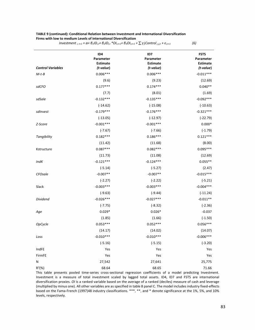
83
TABLE 9 (continued): Conditional Relation between Investment and International Diversification Firms with low to medium Levels of international Diversification
Investment i, t+1 = α+ β1IDi,t+ β2IDi,t *OIi,t+1+ β3OIi,t+1 + ∑ 𝛾𝑗Control, j,j,t + εi,t+1 (6)
ID4 ID7 FSTS
Control Variables
Parameter Estimate (t-value)
Parameter Estimate (t-value)
Parameter Estimate (t-value)
M-t-B 0.006*** 0.006*** -0.011***
(9.6) (9.23) (12.69)
sdCFO 0.177*** 0.174*** 0.040**
(7.7) (8.01) (1.69)
sdSale -0.132*** -0.135*** -0.092***
(-14.62) (-15.08) (-10.63)
sdInvest -0.179*** -0.176*** -0.321***
(-13.05) (-12.97) (-22.79)
Z-Score -0.001*** -0.001*** 0.000*
(-7.67) (-7.66) (-1.79)
Tangibility 0.182*** 0.186*** 0.121***
(11.42) (11.68) (8.00)
Kstructure 0.087*** 0.082*** 0.095***
(11.73) (11.08) (12.69)
IndK -0.121*** -0.124*** 0.055**
(-5.14) (-5.27) (2.47)
CFOsale -0.007** -0.007** -0.015***
(-2.27) (-2.22) (-5.21)
Slack -0.003*** -0.003*** -0.004***
(-9.63) (-9.44) (-11.24)
Dividend -0.026*** -0.027*** -0.011**
(-7.75) (-8.32) (-2.36)
Age 0.029* 0.026* -0.037
(1.85) (1.66) (-1.50)
OpCycle 0.053*** 0.052*** 0.056***
(14.17) (14.02) (14.07)
Loss -0.010*** -0.010*** -0.006***
(-5.16) (-5.15) (-3.20)
IndFE Yes Yes Yes
FirmFE Yes Yes Yes
N 27,542 27,641 25,775
R2(%) 68.64 68.65 71.66 This table presents pooled time-series cross-sectional regression coefficients of a model predicting Investment. Investment is a measure of total investment scaled by lagged total assets. ID4, ID7 and FSTS are international diversification proxies. OI is a ranked variable based on the average of a ranked (deciles) measure of cash and leverage (multiplied by minus one). All other variables are as specified in table 8 panel C. The model includes industry fixed-effects based on the Fama-French (1997)48 industry classifications. ***, **, and * denote significance at the 1%, 5%, and 10% levels, respectively.
84
Regarding the corporate governance variables, the estimated coefficients on the main
effects are positive for institution ownership. InvGscore and analyst following are negative and
against prediction. For the interactions between corporate governance and OI, the estimate
coefficient for both analysts and invGscore are positive. This suggests that analyst following, and
shareholder protections are ineffective at preventing overinvestment in settings where a firm is
more likely to overinvest. The interaction between institutions and OI is negative. Suggesting that
institutional ownership is effective in curtailing overinvestment in settings where firms are more
likely to over-invest.
5.2.2.2 Conditional tests: firms with higher levels of international diversification
Hypotheses 2c and 2d tests the relation between international diversification and
investment efficiency for firms with higher levels of diversification. Table 10 reports the results
for this analysis. For these firms, I find evidence that international diversification is negatively
associated with investment among firms with higher likelihood of under-investing. The estimated
coefficient of international diversification is significant for both the ID4 and ID7 measure. The t-
values are -5.1 and -5.02 for ID4 and ID7, respectively. FSTS is not significant. The negative
associations between both ID4 and ID7 are in line with hypothesis 2d. The coefficient of ID4(ID7)
is significant with a t-statistic of -5.01. Increasing ID4 by one standard deviation, increases
investment by approximately 4.41% (4.51%). For FSTS both the main effect and the interaction
are insignificant.
For the interaction between international diversification and over-investment, the
estimated coefficients are positive and significant for both ID4 and ID7 with t-statistics of 6.0 and

85
5.69, respectively. Increasing ID4(ID7) by one standard deviation, leads to an increase in
overinvestment by 10.66% (10.51%). The sum of the coefficients of ID measure and the
interaction between international diversification and OI captures the overall effect of
international diversification on investment among firms that are over-investing. For both
ID4 and ID7, the sum is positive and significant. This finding offers support for hypothesis 2c.
For corporate governance variables, the estimated coefficients on the main effects are
positive for analyst following in the case of ID4 and ID7 only. Contrary to predictions, the
coefficients of InvGscore and institutional ownership are negative in the case of ID4 and ID7.
This suggest that institutional mechanisms are less effective in preventing under-investment
in firms with higher levels of international diversification. Coefficients of InvGscore and
institutional ownership are positive in the case of FSTS. For the interactions between
corporate governance and OI, the estimate coefficient for both institutions and invGscore
are positive in the case of ID4 and ID7. This suggests that institutional monitoring and
shareholder protections are ineffective at preventing overinvestment in settings where a
firm is more likely to overinvest. The interaction between analysts and OI is negative in the
ID4 and ID7 results. For FSTS the coefficient of the interaction of InvGScore and OI is negative
and consistent with predictions.
In additional analyses47, I rerun the model with FSTS and exclude CYSE and InvDBScore.
The result for the coefficient of FSTS remains insignificant and fails to offer support for
hypotheses 2c and 2d.
47 Appendix 4
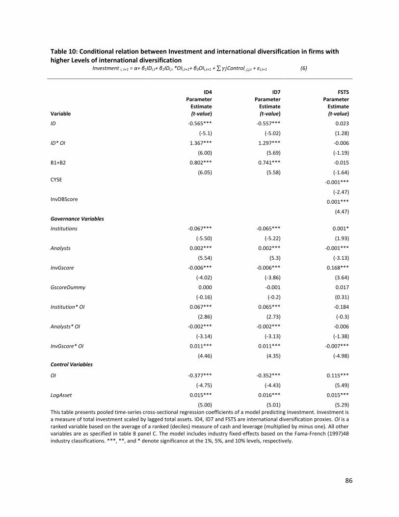
86
Table 10: Conditional relation between Investment and international diversification in firms with higher Levels of international diversification
Investment i, t+1 = α+ β1IDi,t+ β2IDi,t *OIi,t+1+ β3OIi,t+1 + ∑ 𝛾𝑗Control, j,j,t + εi,t+1 (6)
ID4 ID7 FSTS
Variable
Parameter Estimate (t-value)
Parameter Estimate (t-value)
Parameter Estimate (t-value)
ID -0.565*** -0.557*** 0.023
(-5.1) (-5.02) (1.28)
ID* OI 1.367*** 1.297*** -0.006
(6.00) (5.69) (-1.19)
B1+B2 0.802*** 0.741*** -0.015
(6.05) (5.58) (-1.64) CYSE -0.001*** (-2.47) InvDBScore 0.001***
(4.47) Governance Variables
Institutions -0.067*** -0.065*** 0.001*
(-5.50) (-5.22) (1.93)
Analysts 0.002*** 0.002*** -0.001***
(5.54) (5.3) (-3.13)
InvGscore -0.006*** -0.006*** 0.168***
(-4.02) (-3.86) (3.64)
GscoreDummy 0.000 -0.001 0.017
(-0.16) (-0.2) (0.31)
Institution* OI 0.067*** 0.065*** -0.184
(2.86) (2.73) (-0.3)
Analysts* OI -0.002*** -0.002*** -0.006
(-3.14) (-3.13) (-1.38)
InvGscore* OI 0.011*** 0.011*** -0.007***
(4.46) (4.35) (-4.98)
Control Variables
OI -0.377*** -0.352*** 0.115***
(-4.75) (-4.43) (5.49)
LogAsset 0.015*** 0.016*** 0.015***
(5.00) (5.01) (5.29) This table presents pooled time-series cross-sectional regression coefficients of a model predicting Investment. Investment is a measure of total investment scaled by lagged total assets. ID4, ID7 and FSTS are international diversification proxies. OI is a ranked variable based on the average of a ranked (deciles) measure of cash and leverage (multiplied by minus one). All other variables are as specified in table 8 panel C. The model includes industry fixed-effects based on the Fama-French (1997)48 industry classifications. ***, **, and * denote significance at the 1%, 5%, and 10% levels, respectively.
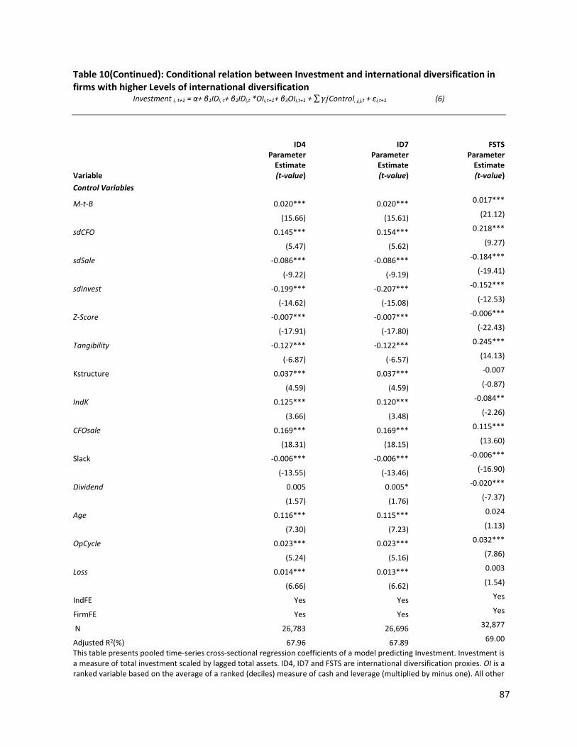
87
Table 10(Continued): Conditional relation between Investment and international diversification in firms with higher Levels of international diversification
Investment i, t+1 = α+ β1IDi, t+ β2IDi,t *OIi,t+1+ β3OIi,t+1 + ∑ 𝛾𝑗Control, j,j,t + εi,t+1 (6)
ID4 ID7 FSTS
Variable
Parameter Estimate (t-value)
Parameter Estimate (t-value)
Parameter Estimate (t-value)
Control Variables
M-t-B 0.020*** 0.020*** 0.017***
(15.66) (15.61) (21.12)
sdCFO 0.145*** 0.154*** 0.218***
(5.47) (5.62) (9.27)
sdSale -0.086*** -0.086*** -0.184***
(-9.22) (-9.19) (-19.41)
sdInvest -0.199*** -0.207*** -0.152***
(-14.62) (-15.08) (-12.53)
Z-Score -0.007*** -0.007*** -0.006***
(-17.91) (-17.80) (-22.43)
Tangibility -0.127*** -0.122*** 0.245***
(-6.87) (-6.57) (14.13)
Kstructure 0.037*** 0.037*** -0.007
(4.59) (4.59) (-0.87)
IndK 0.125*** 0.120*** -0.084**
(3.66) (3.48) (-2.26)
CFOsale 0.169*** 0.169*** 0.115***
(18.31) (18.15) (13.60)
Slack -0.006*** -0.006*** -0.006***
(-13.55) (-13.46) (-16.90)
Dividend 0.005 0.005* -0.020***
(1.57) (1.76) (-7.37)
Age 0.116*** 0.115*** 0.024
(7.30) (7.23) (1.13)
OpCycle 0.023*** 0.023*** 0.032***
(5.24) (5.16) (7.86)
Loss 0.014*** 0.013*** 0.003
(6.66) (6.62) (1.54)
IndFE Yes Yes Yes
FirmFE Yes Yes Yes
N 26,783 26,696 32,877
Adjusted R2(%) 67.96 67.89 69.00
This table presents pooled time-series cross-sectional regression coefficients of a model predicting Investment. Investment is a measure of total investment scaled by lagged total assets. ID4, ID7 and FSTS are international diversification proxies. OI is a ranked variable based on the average of a ranked (deciles) measure of cash and leverage (multiplied by minus one). All other

88
variables are as specified in table 8 panel C. The model includes industry fixed-effects based on the Fama-French (1997)48 industry classifications. ***, **, and * denote significance at the 1%, 5%, and 10% levels, respectively.
5.2.3 Unconditional tests of the relation between international diversification and investment
efficiency
Tests in the prior section were conditional on the firm being in settings where under-or over-
investment are more likely. In this section, I directly examine the association between
international diversification and the likelihood of under and over-investment. I classify firms into
three investment groups (inv_gp) depending on the quartiles of residuals from equation (5).
Firms in the bottom quartile of the distribution are classified as under-investing as the have the
lowest residual. These firms are placed in the middle group (Inv_gp=1). Firms in the two middle
quartiles of the residual are placed in group 2(Inv_gp=2) and treated as the control group
(Inv_gp=2). Firms in the top quartile of the residual are classified as overinvesting and are placed
in group 3 (Inv_gp=3).
I estimate a multinomial logistic regression that tests the likelihood that a firm might be in the
extreme investment residual quartiles as a function of international diversification. In the model
specification, I consider simultaneously, but separately the likelihood of over- and under -
investment.
5.2.3.1 Unconditional tests: firms with low to medium levels of international diversification.
Tables 11 and 12 present results for forms with low to medium levels of international
diversification. Table 11 presents results regarding underinvestment. The coefficients of ID4, ID7
and FSTS are negative and statistically significant at the 1 percent level. Hypothesis 2b, predicts
89
a negative relation between international diversification and under-investment. This result is
in support of hypotheses 2b. For the governance variables, analyst following is negatively
associated with underinvestment. Institutional ownership is positively associated with the
likelihood that a firm will underinvestment in. The coefficients of InvGScore is positive in the
ID4 and ID7 analyses but negative in the FSTS analysis.
Table 12 presents the results of the analyses regarding overinvestment versus normal
investment. The coefficients of ID4, ID7 and FSTS have the predicted sign. However, none of
the coefficients is significant. Hypothesis 2a predicts that for firms with low to medium levels
of international diversification, there is a negative association between international
diversification and over investment. The insignificant results fail to lend support for this
prediction.
Considering the governance variables, institutional ownership is positively associated with
the likelihood of over-investment when ID4 and ID7 are the proxies for international
diversification. When FSTS is the proxy, institutional ownership is negatively associated with
the likelihood of overinvestment. Analyst coverage is insignificant in all three analyses.
InvGscore is insignificant in the analyses where ID4 and ID7 are used as the proxies for
international diversification. In the analysis using FSTS, InvGscore is significant and negatively
associated with the likelihood of overinvestment.
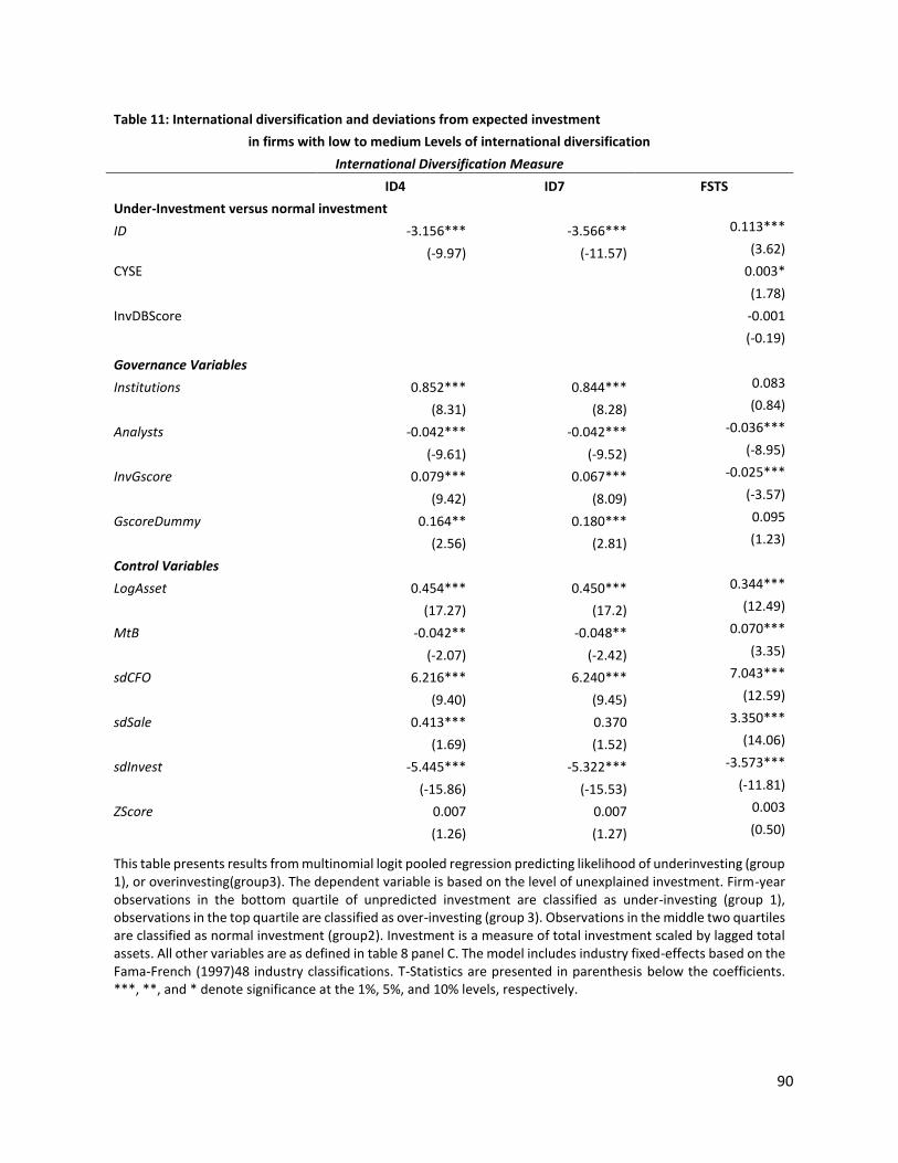
90
Table 11: International diversification and deviations from expected investment
in firms with low to medium Levels of international diversification
International Diversification Measure
ID4 ID7 FSTS
Under-Investment versus normal investment
ID -3.156*** -3.566*** 0.113***
(-9.97) (-11.57) (3.62)
CYSE 0.003*
(1.78)
InvDBScore -0.001
(-0.19)
Governance Variables
Institutions 0.852*** 0.844*** 0.083
(8.31) (8.28) (0.84)
Analysts -0.042*** -0.042*** -0.036***
(-9.61) (-9.52) (-8.95)
InvGscore 0.079*** 0.067*** -0.025***
(9.42) (8.09) (-3.57)
GscoreDummy 0.164** 0.180*** 0.095
(2.56) (2.81) (1.23)
Control Variables
LogAsset 0.454*** 0.450*** 0.344***
(17.27) (17.2) (12.49)
MtB -0.042** -0.048** 0.070***
(-2.07) (-2.42) (3.35)
sdCFO 6.216*** 6.240*** 7.043***
(9.40) (9.45) (12.59)
sdSale 0.413*** 0.370 3.350***
(1.69) (1.52) (14.06)
sdInvest -5.445*** -5.322*** -3.573***
(-15.86) (-15.53) (-11.81)
ZScore 0.007 0.007 0.003
(1.26) (1.27) (0.50)
This table presents results from multinomial logit pooled regression predicting likelihood of underinvesting (group 1), or overinvesting(group3). The dependent variable is based on the level of unexplained investment. Firm-year observations in the bottom quartile of unpredicted investment are classified as under-investing (group 1), observations in the top quartile are classified as over-investing (group 3). Observations in the middle two quartiles are classified as normal investment (group2). Investment is a measure of total investment scaled by lagged total assets. All other variables are as defined in table 8 panel C. The model includes industry fixed-effects based on the Fama-French (1997)48 industry classifications. T-Statistics are presented in parenthesis below the coefficients. ***, **, and * denote significance at the 1%, 5%, and 10% levels, respectively.
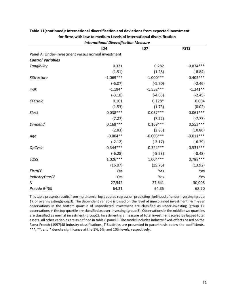
91
Table 11(continued): International diversification and deviations from expected investment
for firms with low to medium Levels of international diversification
International Diversification Measure
ID4 ID7 FSTS
Panel A: Under-Investment versus normal investment
Control Variables
Tangibility 0.331 0.282 -0.874***
(1.51) (1.28) (-8.84)
KStructure -1.069*** -1.000*** -0.402***
(-6.07) (-5.70) (-2.46)
indk -1.184* -1.552*** -1.241**
(-3.10) (-4.05) (-2.45)
CFOsale 0.101 0.128* 0.004
(1.53) (1.73) (0.02)
Slack 0.038*** 0.037*** -0.061***
(7.27) (7.22) (-7.77)
Dividend 0.168*** 0.169*** 0.553***
(2.83) (2.85) (10.86)
Age -0.004** -0.006*** -0.011***
(-2.12) (-3.17) (-6.39)
OpCycle -0.344*** -0.324*** -0.531***
(-6.28) (-5.93) (-8.48)
LOSS 1.026*** 1.004*** 0.788***
(16.07) (15.76) (13.92)
FirmFE Yes Yes Yes
IndustryYearFE Yes Yes Yes
N 27,542 27,641 30,008
Pseudo R2(%) 64.21 64.35 68.20
This table presents results from multinomial logit pooled regression predicting likelihood of underinvesting (group 1), or overinvesting(group3). The dependent variable is based on the level of unexplained investment. Firm-year observations in the bottom quartile of unpredicted investment are classified as under-investing (group 1), observations in the top quartile are classified as over-investing (group 3). Observations in the middle two quartiles are classified as normal investment (group2). Investment is a measure of total investment scaled by lagged total assets. All other variables are as defined in table 8 panel C. The model includes industry fixed-effects based on the Fama-French (1997)48 industry classifications. T-Statistics are presented in parenthesis below the coefficients. ***, **, and * denote significance at the 1%, 5%, and 10% levels, respectively.

92
Table 12: International diversification and deviations from expected investment for firms with low to medium levels of international diversification
International Diversification Proxy
ID4 ID7 FSTS
Overinvestment versus normal investment ID -0.217 -0.455 -0.021
(-0.66) (-1.43) (-0.33)
CYSE -0.035***
(-17.15)
InvDBScore -0.006*
(-1.81)
Institutions 0.503*** 0.538*** -0.449***
(4.91) (5.26) (-4.41)
Analysts 0.001 0.003 -0.006
(0.12) (0.78) (-1.3)
InvGscore 0.001 -0.005 -0.016*
(0.17) (-0.59) (-1.84)
GscoreDummy -0.015 -0.016 0.122
(-0.25) (-0.26) (1.56)
logAsset -0.110*** -0.119*** 0.012
(-4.08) (-4.41) (0.37)
MtB 0.024 0.017 0.231***
(1.25) (0.91) (10.86)
sdCFO 10.618*** 10.760*** 7.335***
(16.05) (16.22) (11.18)
sdSale -3.135*** -3.205*** -0.791***
(-11.73) (-12.00) (-2.75)
sdInvest 3.086*** 3.185*** 3.137***
(8.70) (8.98) (9.73)
Z_Score 0.002 0.002 -0.029***
(0.37) (0.42) (-4.25)
Tangibility 2.565*** 2.501*** 3.539***
(13.11) (12.76) (16.64)
This table presents results from multinomial logit pooled regression predicting likelihood of underinvesting (group 1), or overinvesting(group3). The dependent variable is based on the level of unexplained investment. Firm-year observations in the bottom quartile of unpredicted investment are classified as under-investing (group 1), observations in the top quartile are classified as over-investing (group 3). Observations in the middle two quartiles are classified as normal investment (group2). Investment is a measure of total investment scaled by lagged total assets. All other variables are as defined in table 8 panel C. The model includes industry fixed-effects based on the Fama-French (1997)48 industry classifications. T-Statistics are presented in parenthesis below the coefficients. ***, **, and * denote significance at the 1%, 5%, and 10% levels, respectively.

93
Table 12(continued): International diversification and deviations from expected investment for firms with low to medium levels of international diversification
International Diversification Proxy
ID4 ID7 FSTS
Overinvestment versus normal investment
KStructure -0.975*** -0.894*** -2.836***
(-5.97) (-5.49) (-14.36)
Indk 1.119*** 1.088*** 1.282***
(3.25) (3.17) (2.77)
CFOsale 0.155*** 0.151*** -0.767***
(3.45) (3.44) (-3.35)
Slack -0.089*** -0.091*** -0.077***
(-8.02) (-8.09) (-8.18)
Dividend -0.193*** -0.199*** -0.239***
(-3.45) (-3.56) (-4.13)
Age -0.019*** -0.019*** -0.014***
(-11.17) (-11.19) (-7.85)
OpCycle 0.029 0.037 0.450***
(0.49) (0.63) (6.71)
LOSS 0.286*** 0.264*** 0.671***
(4.54) (4.19) (10.59)
FirmFE Yes Yes Yes
IndustryYearFE Yes Yes Yes
N 27,542 27,641 30,008
Pseudo R2(%) 64.21 64.35 68.20 This table presents results from multinomial logit pooled regression predicting likelihood of underinvesting (group 1) and overinvesting (group 3). The dependent variable is based on the level of unexplained investment. Firm-year observations in the bottom quartile of unpredicted investment are classified as under-investing (group 1), observations in the top quartile are classified as over-investing (group 3). Observations in the middle two quartiles are classified as normal investment (group2). Investment is a measure of total investment scaled by lagged total assets. All other variables are as defined in table 8 panel C. The model includes industry fixed-effects based on the Fama-French (1997)48 industry classifications. T-Statistics are presented in parenthesis below the coefficients. ***, **, and * denote significance at the 1%, 5%, and 10% levels, respectively.
94
5.2.3.2 Unconditional tests: firms with higher levels of international diversification.
Tables 13 and Tables 14 present results for firms with higher levels of international
diversification. Table 13 presents results regarding underinvestment. Consistent with predictions
the three coefficients of ID are positive and significant. Hypothesis 2d predicts a positive
association between international diversification and under-investment for firms with higher
levels of diversification. The results in table 13 are consisted with hypothesis 2d as the
coefficients of ID are all positive and significant 1 percent level. That is, there is evidence of
suboptimal investment, with a tendency to under-investment as firms’ levels of diversifications
increase.
For the governance variables, analyst following is negatively associated with underinvestment
in all three cases. When the international diversification measure is ID4 and FSTS, Institutional
ownership is negatively associated with the likelihood that a firm will underinvest. This is
consistent with corporate governance mitigating under-investment. When ID7 is the
international diversification measure, institutional ownership is positively associated with the
likelihood of underinvestment. InvGscore is positively associated with the likelihood that a firm
will underinvest.
In additional analysis, I rerun the FSTS regression without CYSE and InvDBScore in the model.
The results are presented in Appendix 7. This results in positive and significant coefficient for
FSTS. This offers further support to hypothesis 2d.

95
Table 13: International diversification and deviations from expected investment for firms with higher Levels of international diversification
ID4 ID7 FSTS Underinvestment versus normal investment ID 6.572*** 1.769*** 0.761*** (6.82) (6.89) (4.54) CYSE -0.002 (-1.49) InvDBScore -0.029*** (-10.56) Institutions -0.868*** 0.257*** -0.102
(-8.41) (3.12) (-1.05)
Analysts -0.011** -0.058*** -0.491***
(-2.41) (-15.54) (-10.44)
InvGscore 0.046*** 0.018*** 0.081***
(6.12) (2.66) (9.61)
GscoreDummy -0.077 -0.169*** -0.004
(-0.63) (-3.04) (-0.06)
logAsset 0.246*** 0.435*** 0.462***
(8.93) (19.24) (15.02)
MtB -0.406*** -0.011 -0.258***
(-14.65) (-0.58) (-11.03)
sdCFO 7.757*** 1.681*** 3.633***
(11.3) (3.4) (5.82)
sdSale -0.106 0.508*** -2.216***
(-0.45) (3.04) (-9.39)
sdInvest -1.762*** -2.625*** -7.034***
(-5.14) (-8.97) (-19.49)
Z_Score 0.084*** 0.011** 0.051***
(10.71) (2.29) (8.23)
Tangibility -2.523*** -0.866*** -0.300
(-11.72) (-4.97) (-1.39) This table presents results from multinomial logit pooled regression predicting likelihood of underinvesting (group 1) and overinvesting (group 3). The dependent variable is based on the level of unexplained investment. Firm-year observations in the bottom quartile of unpredicted investment are classified as under-investing (group 1), observations in the top quartile are classified as over-investing (group 3). Observations in the middle two quartiles are classified as normal investment group (group2). Investment is a measure of total investment scaled by lagged total assets. All other variables are as specified in table 8 panel C. The model includes industry fixed-effects based on the Fama-French (1997)48 industry classifications. T-Statistics are presented in parenthesis below the coefficients. ***, **, and * denote significance at the 1%, 5%, and 10% levels, respectively.

96
Table 13(continued): international diversification and deviations from expected investment for firms with higher levels of international diversification
international diversification proxy
ID4 ID7 FSTS Underinvestment versus normal investment KStructure -0.392** -1.207*** -0.483***
(-2.45) (-8.64) (-3.01)
Indk -4.352*** -2.066*** -3.093***
(-8.14) (-6.44) (-8.36)
CFOsale -0.656*** -0.023 -0.018
(-3.59) (-0.55) (-0.43)
Slack -0.060*** 0.015*** 0.047***
(-6.68) (3.93) (8.08)
Dividend -0.070 0.020 -0.155***
(-1.34) (0.4) (-2.56)
Age 0.027*** 0.005*** 0.005***
(15.43) (3.39) (2.86)
OpCycle -0.449*** -0.331*** -0.225***
(-7.05) (-7.05) (-4.00)
Loss 0.375*** 0.612*** 0.658***
(6.28) (11.89) (10.39)
FirmFE Yes Yes Yes
IndustryYearFE Yes Yes Yes
N 26,783 26,696 26,985
Pseudo R2(%) 68.49 68.14 64.91 This table presents results from multinomial logit pooled regression predicting likelihood of underinvesting (group 1) and overinvesting (group 3). The dependent variable is based on the level of unexplained investment. Firm-year observations in the bottom quartile of unpredicted investment are classified as under-investing (group 1), observations in the top quartile are classified as over-investing (group 3). Observations in the middle two quartiles are classified as normal investment group (group2). Investment is a measure of total investment scaled by lagged total assets. All other variables are as specified in table 8 panel C. The model includes industry fixed-effects based on the Fama-French (1997)48 industry classifications. T-Statistics are presented in parenthesis below the coefficients. ***, **, and * denote significance at the 1%, 5%, and 10% levels, respectively.
Table 14 presents the results of the analyses regarding overinvestment. Consistent with
predictions, the coefficients of ID4, ID7 and FSTS are all positive. They are all significant with

97
Table 14: International diversification and deviations from expected investment in firms with higher Levels of international diversification International Diversification Proxy
ID4 ID7 FSTS Overinvestment versus normal investment ID 3.138*** 0.665** 1.055*** (2.87) (2.51) (6.12) CYSE 0.000 (0.05) InvDBScore 0.003 (1.14)
Institutions -1.104*** -0.255*** 0.147
(-10.07) (-3.02) (1.51)
Analysts 0.067*** -0.004 0.013***
(13.49) (-1.16) (2.71)
InvGscore 0.055*** 0.000 0.021**
(5.86) (-0.01) (2.41)
GscoreDummy -0.040 -0.051 0.008
(-0.31) (-0.93) (0.11)
logAsset -0.521*** -0.105*** -0.258***
(-15.27) (-4.32) (-8.14)
MtB 0.020 0.020 -0.013
(0.71) (1.12) (-0.66)
sdCFO 9.633*** 6.253*** 7.796***
(12.41) (12.39) (12.76)
sdSale -2.013*** -2.605*** -2.268***
(-7.16) (-12.7) (-9.59)
sdInvest 3.370*** 4.546*** 1.729***
(9.50) (15.47) (5.02)
Z_Score 0.015* 0.006 0.015**
(1.68) (1.31) (2.41)
Tangibility 3.594*** 2.056*** 2.687***
(16.25) (12.42) (14.1) This table presents results from multinomial logit pooled regression predicting likelihood of underinvesting (group 1) and overinvesting (group 3). The dependent variable is based on the level of unexplained investment. Firm-year observations in the bottom quartile of unpredicted investment are classified as under-investing (group 1), observations in the top quartile are classified as over-investing (group 3). Observations in the middle two quartiles are classified as normal investment group (group2). Investment is a measure of total investment scaled by lagged total assets. All other variables are as specified in table 8 panel C. The model includes industry fixed-effects based on the Fama-French (1997)48 industry classifications. T-Statistics are presented in parenthesis below the coefficients. ***, **, and * denote significance at the 1%, 5%, and 10% levels, respectively.

98
Table 14(continued): International diversification and deviations from expected investment in firms with higher Levels of international diversification International Diversification Proxy
ID4 ID7 FSTS Overinvestment versus normal investment KStructure -1.396*** -1.178*** -0.085
(-6.88) (-8.55) (-0.56)
Indk 1.121** 0.470 -0.779**
(2.02) (1.51) (-2.22)
CFOsale -0.507*** 0.122*** 0.149***
(-2.64) (3.11) (3.55)
Slack -0.020** -0.061*** -0.047***
(-2.24) (-8.18) (-5.32)
Dividend 0.363*** -0.390*** 0.225
(6.01) (-8.1) (3.90)
Age -0.004** -0.005*** -0.022***
(-2.14) (-3.08) (-13.03)
OpCycle 0.862*** 0.331*** 0.548***
(11.83) (6.72) (9.61)
LOSS 0.624*** 0.112** -0.014
(8.77) (2.06) (-0.22)
FirmFE Yes Yes Yes
IndustryYearFE Yes Yes Yes
N 26,783 26,696 26,985
Pseudo R2(%) 68.49 68.14 64.91 This table presents results from multinomial logit pooled regression predicting likelihood of underinvesting (group 1) and overinvesting (group 3). The dependent variable is based on the level of unexplained investment. Firm-year observations in the bottom quartile of unpredicted investment are classified as under-investing (group 1), observations in the top quartile are classified as over-investing (group 3). Observations in the middle two quartiles are classified as normal investment group (group2). Investment is a measure of total investment scaled by lagged total assets. All other variables are as specified in table 8 panel C. The model includes industry fixed-effects based on the Fama-French (1997)48 industry classifications. T-Statistics are presented in parenthesis below the coefficients. ***, **, and * denote significance at the 1%, 5%, and 10% levels, respectively.
t-values ranging from 2.51 for ID7 to 6.12 for FSTS. This lends support for hypothesis 2c.
Considering governance variables, institutional ownership is negatively associated with the
likelihood of overinvestment in the ID4 and ID7 analyses. Analyst coverage is positively associated
99
with overinvestment when ID4 and ID7 are the proxies for international diversification. This
suggests that there is ineffectiveness in mitigating over-investment. InvGscore is insignificant in
the analyses where ID7 and FSTS are used as the proxies for international diversification. In the
analysis using ID4, InvGscore is significant and positively associated with the likelihood of
overinvestment. This is consistent with ineffectiveness of shareholder protections in mitigating
suboptimal investment for firms with higher levels of international diversification.
In additional analyses, I ran the FSTS analysis without CYSE and InvDBScore. The results
are presented in appendix 7. The coefficients are consistent with the results in the main analyses.
5.3 Research and Development Intensity -Results of Hypothesis Tests
5.3.1 Sample and descriptive statistics for R&D intensity
The sample consist of manufacturing firms from Compustat from 1990-2019.
International diversification data is calculated based on COMPUSTAT segment files. Table
15 presents the descriptive statistics of the sample used in the analysis of the association
between research and development intensity and the degree of international
diversification. The sample consists of 184,082 firm-year observations for regressions
using FSTS (Foreign to total sales) as the international diversification measure and
152,080 and 152,098 firm-observations for analyses using ID4 and ID748 respectively, to
48 ID4 and ID7 are constructed using the Hitt et al. (1997) ID4 is based on the four regions used in Hitt et al. (1997). ID7 is based on the seven-region classification by the World Bank. The seven regions are East Asia and Pacific, Europe and Central Asia, Latin America and the Caribbean, Middle East and North Africa, North America, South Asia, and Sub-Saharan Africa.

100
proxy international diversification. Financial information data is from Compustat. Continuous
variables are winsorized at the 1% and 99% levels.
Table 15: Research and development intensity- Descriptive Statistics
Variable N Mean Median Q1 Q3 Std Dev RNDI 184,082 23.155 6.889 2.473 23.702 41.283 ID4 152,080 0.280 0.298 0.240 0.339 0.075 ID7 152,098 0.277 0.296 0.234 0.339 0.079
FSTS 184,082 0.484 0.481 0.323 0.644 0.237 LnRev 184,082 7.611 7.675 6.516 8.867 1.740 DEBT 184,082 0.233 0.220 0.106 0.326 0.175 MA 184,082 0.243 0.000 0.000 0.000 4.155 CYSE 184,082 26.199 23.000 11.000 37.000 19.017 InvDBScore 146,984 18.225 18.575 13.495 114.000 6.848 Subsidiaries 184,082 90.979 53.000 21.000 115.000 112.285

101
Table 16: Research and Development Intensity -Pearson Correlation Coefficients
Prob > |r| under H0: Rho=0
RNDI ID4 ID7 FSTS LnRev Debt MA CYSE Subs
RNDI 1.000
ID4 0.032 1.000
<.0001
ID7 0.040 0.975 1.000
<.0001 <.0001
FSTS 0.096 0.388 0.377 1.000
<.0001 <.0001 <.0001
LnRev -0.095 0.047 0.046 0.089 1.000
<.0001 <.0001 <.0001 <.0001
Debt -0.092 -0.025 -0.024 -0.101 0.094 1.000
<.0001 <.0001 <.0001 <.0001 <.0001
MA -0.004 -0.062 -0.063 0.001 0.019 0.004 1.000
0.183 <.0001 <.0001 0.746 <.0001 0.141
CYSE -0.054 0.082 0.087 0.145 0.714 0.056 0.024 1.000
<.0001 <.0001 <.0001 <.0001 <.0001 <.0001 <.0001
Subs -0.073 0.038 0.038 0.109 0.585 0.032 0.042 0.803 1.000
<.0001 <.0001 <.0001 <.0001 <.0001 <.0001 <.0001 <.0001 ID4 is the international diversification constructed following Hitt et al. (1997) procedure, using four economic world regions. ID7 is the international diversification constructed following Hitt et al. (1997) procedure, using seven economic world regions as identified by the World Bank in its economic reports. FSTS is the ratio of total foreign sales to total sales. RNDI is the ratio of R&D cost to the number of employees. Debt is the ratio of leverage to total assets *-1. LnRev is the natural log of sales. MA is the number of mergers and acquisitions undertaken during the year. CYSE is the country scope, that is the number of countries in which the firm operations. Subs is the number of firm subsidiaries,
Table 15 presents descriptive statistics for the variables used in the analyses of
research and development intensity. The mean(median) research and development per
employee is RNDI is 23.965 (6.889). The mean(median) ID4 is 0.280(0.298) respectively.
The mean(median) ID7 is 0.277 (0.296). The mean(median) FSTS is 0.481(0.481). The
median and mean number of countries (CYSE) in which the sample firms operate is 26 and
23 respectively. The mean and median number of subsidiaries is 91 and 53 respectively.
Table 16, panel A, presents the correlations among the variables. ID4 and ID7 are
significantly correlated with a rate of 0.98. FSTS has a lower correlation with both ID4 and ID7.
102
The correlation rate is significant at 0.39 and 0.38 respectively. ID4 and ID7 capture both the
breadth and the width of firms’ international diversification activities. FSTS captures only the
ratio of foreign sales to total firm sales. RNDI is positively correlated with all three international
diversification measures. RNDI is not significantly correlated with number of mergers and
acquisitions (MA). RNDI is negatively associated with both the number of countries in which a
firm operates (CYSE) and the number of subsidiaries (Subs).
5.3.2 Results for Research and Development Intensity
Table 17 presents the results for fixed effects analysis of the relationship between
international diversification and research and development intensity. For all three proxies, the
coefficient of international diversification is positively significant at a 1% level. The t-values range
from 5.35 for FSTS to 6.01 in the case of ID7. This shows that as the level of international
diversification increases research and development intensity increases. Hypothesis 3 is non
directional due to the existence of dynamics between international diversification and
innovation. Further, prior studies point to a dynamic interplay between international activities,
organizational learning, and innovations (e.g., Gkypali et al. 2021). The positive finding is
consistent with greater effects from factors that promote greater R&D intensity as firms
internationally diversify. For instance, the existence of diverse markets, and the need for
adapting products to the market demands may push firms to invest more in R&D resources. The
positive result is also consistent with findings in prior research (Hitt et al. 1997; Baysinger and
Hoskisson, 1989; Hoskisson & Hitt, 1988). In economic terms, a one standard deviation increase
in ID4(ID7), leads to a 0.51% (0.50%) increase in R&D expenditure per employee. Given that the

103
average expenditure per employee is 23,155, this represents an increase of $21.78 ($21.45) per
employee.
The coefficient of LnRev is negatively significant in all three cases. This can be due to firms
with higher sales having less need to invest in R&D, having become well established in their
respective markets. Debt is positively significant at the one percent level. The positive
significance could suggest that firms could be using more debt to get funds, with part of the
proceeds going to R&D research. The coefficient of CYSE, country scope is negatively significant.
This suggests as companies operate in a greater number of countries, they invest less in R&D
dollars per employee. It lends to arguments in prior literature that firms may substitute
diversification for innovation (e.g., Banker et al., 2011).
In additional analysis, I run OLS regressions. The results are presented in table 18.
Like prior results, the coefficient of ID is positive and significant at the 1 percent level.
However, the R2 is incredibly low in the OLS regression. This suggests that there are
omitted variables that explain the degree of research and development intensity in
internationally diversified firms.

104
TABLE 17: Fixed effects- Relation between international diversification and research and development intensity
International diversification proxy
ID4 ID7 FSTS
Variable Parameter Estimate (t-value)
Parameter Estimate (t-value)
Parameter Estimate (t-value)
ID 6.727*** 6.826*** 0.987***
(5.66) (6.01) (5.35)
LnRev -1.766*** -1.770*** -1.442***
(-7.84) (-7.86) (-7.56)
DEBT 6.218*** 6.220*** 5.475***
(10.59) (10.6) (11.22)
MA 0.005 0.005 0.004
(0.55) (0.54) (0.5)
CYSE -0.253*** -0.254*** -0.157***
(-14.23) (-14.26) (-10.98)
Subsidiaries 0.017*** 0.017*** 0.010***
(8.84) (8.86) (6.22)
FirmFE Yes Yes Yes
IndYrFE Yes Yes Yes
N 152,080 152,098 184,082
Adjusted R2(%) 79.5 79.5 79.8
This table presents fixed effects regression coefficients of a model predicting research and development intensity. ID is the international diversification measure. ID4 is the international diversification constructed following Hitt et al. (1997) procedure, using four economic world regions. ID7 is the international diversification constructed following Hitt et al. (1997) procedure, using seven economic world regions as identified by the World Bank in its economic reports49. FSTS is the ratio of total foreign sales to total sales. RNDI is the ratio of R&D cost to the number of employees. Debt is the ratio of leverage to total assets *-1. LnRev is the natural log of sales. MA is the number of mergers and acquisitions undertaken during the year. CYSE is the country scope, that is the number of countries in which the firm operations. InvDBScore is the inverse of the doing-business score which captures foreign companies’ ease of doing business in the country. The model includes industry fixed-effects based on the Fama-French (1997)48 industry classifications. T-Statistics are presented in parenthesis below the coefficients l. ***, **, and * denote significance at the 1%, 5%, and 10% levels, respectively.
49 https://datahelpdesk.worldbank.org/knowledgebase/articles/378834-how-does-the-world-bank-classify-countries

105
TABLE 18: OLS- Relation between international diversification and research and development intensity
International diversification proxy
ID4 ID7 FSTS
Variable
Parameter Estimate (t-value)
Parameter Estimate (t-value)
Parameter Estimate (t-value)
ID 15.878*** 18.919*** 18.795***
(8.97) (11.43) (31.47)
LnRev -32.609*** -32.562*** -29.423***
(-14.84) (-14.78) (-12.77)
DEBT 0.179*** 0.173*** 0.168***
(-43.34) (-43.28) (-39.01)
MA 0.016 0.017* 0.074
(1.57) (1.95) (-0.36)
CYSE 0.000*** -0.001*** 0.000***
(17.09) (16.42) (15.33)
Subs 0.168*** 0.168*** 0.168***
(-24.27) (-23.99) (-25.98)
InvDBScore 0.017 0.017 0.017***
(1.13) (1.17) (5.20)
FirmYear Cluster Yes Yes Yes
Industry Cluster Yes Yes Yes
N 146,984
146,984 141,842
Adjusted R2(%) 3.34 3.38 4.31 This table presents OLS regression coefficients of a model predicting research and development intensity. ID is the international diversification measure. ID4 is the international diversification constructed following Hitt et al. (1997) procedure, using four economic world regions. ID7 is the international diversification constructed following Hitt et al. (1997) procedure, using seven economic world regions as identified by the World Bank in its economic reports50. FSTS is the ratio of total foreign sales to total sales. RNDI is the ratio of R&D cost to the number of employees. Debt is the ratio of leverage to total assets *-1. LnRev is the natural log of sales. MA is the number of mergers and acquisitions undertaken during the year. CYSE is the country scope, that is the number of countries in which the firm operations. InvDBScore is the inverse of the doing-business score which captures foreign companies’ ease of doing business in the country. The score is reported by World Bank. The model includes clustering by industry based on the Fama-French (1997)48 industry classifications. Heteroscedastic consistent T-Statistics are presented in parenthesis below the coefficients. ***, **, and * denote significance at the 1%, 5%, and 10% levels, respectively. Observations are clustered by firm and year.
50 https://datahelpdesk.worldbank.org/knowledgebase/articles/378834-how-does-the-world-bank-classify-countries

106
Results for sub-sample analyses
To further examine the relationship between international diversification and research
and development intensity, I ran separate analyses for firms that have a low to medium level of
international diversification and those with higher levels of international diversification.
Appendix 8 presents the results for the sample of firms with low to medium levels of
international diversification. For all three proxies of international diversification, the coefficient
of international diversification is positive and significant at the 1% level. The t-values range from
2.71 for ID4 to 5.72 for FSTS. This result is consistent with prior findings for the overall sample. It
suggests that the overall dynamics between international diversification and innovation lead to
a positive relationship between the two factors. These findings can be the result of several
reasons. For example, with increased access to resources as firms diversify internationally, the
economies of scale achieved can have an effect of increasing financial and other resources
available for R&D activities. Similarly, there could be a reverse relationship, where firms that
invest more in R&D, have greater opportunities to expand their international diversification due
to availability of products to offer in various markets.
Consistent with prior finding, the coefficient of debt is positive and significant. The
number of subsidiaries is positively significant in the case of ID4 and ID7 but insignificant when
FSTS is the proxy for international diversification. The coefficient of LnRev is negatively significant
for the first two measures. However, it is positive when FSTS is used as the proxy for international
diversification. The number of countries in which a firm operates is negatively associated with
107
research and development intensity in all three cases. These findings are consistent with the
results for the whole sample.
The results for firms with higher levels of diversification are presented in appendix 9. The
coefficients of ID4 and ID7 are both negative and significant at the 1 percent level. The negative
coefficients for ID4 and ID7 suggest are indicative of a negative association between increases in
ID and investments in R&D per employee. Some of the reasons could be attributed to prior
arguments that instead of investing in R&D, firms sometimes acquire other firms that have the
required technology. Further, firms may have lesser R&D investment needs due to their already
expansive R&D resources and know-how accumulated during their earlier stages of international
diversification. However, the coefficient of FSTS remains positive and significant.
The coefficients of the control variables are mostly similar in direction and significance as
in the case of the analyses using the whole sample and the subsample of firms with low to
medium levels of international diversification.
108
5.4 Uncertainty of Future Benefits from Investments - Results of Hypothesis Tests
5.4.1 Sample and descriptive statistics.
For the sample, I start off with a sample of internationally diversified firms and match it
with financial data from Compustat annual file for the period 1990 to 2019. I retain observations
that have non missing data for the following:
• Capex is the capital expenditures, Compustat data CAPX
• RND is research and development expense, Compustat data XRD. Observations with
missing values are treated as zero, not missing.
• ADEX is the advertising expense, Compustat data XAD. Missing values are set to zero.
• MV is the market value of equity. It is measured as the natural logarithm of the product
of the fiscal year closing price and common shares outstanding, log (PRCC_F*CSHPRI).
• FLEV is financial leverage. It is the sum of long-term debt, DLTT and short-term debt, DLC
divided by the sum of long-term debt and market value of equity.
• E is the earnings per share before ordinary items and discontinued operations
• CF is the cash flow from operations, data OANCF divided by number of common shares
outstanding, CSHPRI
• Sale is sales revenue, divided by the number of common shares
• PRC is the share price
Price per share is measured at the end of year t-1. All the other variables are measured at
year t. For uniformity and comparability with other per share data, future earnings are
adjusted for changes in number of shares using the cumulative adjustment factor, Compustat

109
data AJEX. Earnings sales and cashflow variability are computed using data for 5 years
following year t.
Pandit et al. (2011) and Asdemir et al. (2012) note that research intensive firms are more
likely to engage in mergers and acquisitions and not survive the five- year period required to
calculate variability of future earnings. This causes survivor bias. Consistent with prior literature
(Kothari et al. 2002; Asdemir et al., 2012) for minimizing survivor bias, I do not restrict the sample
to only those observations where there is future benefit data for all consecutive five-year periods.
Following the approach in Asdemir et al. (2012), for a firm to be included in the sample, it must
have complete future benefit data for at least one consecutive five-year period. If a firm is missing
future benefits data for years t+1 to t+5, the standard deviation of future benefits is set equal to
the mean standard deviation of future benefits for firms in the same Altman Z-Score decile
portfolio.
I merge the above Compustat annual data with international diversification data
described previously. International diversification measures is computed using segment data. I
obtain segment sales data from Compustat segment files. Total sales data is obtained from
Compustat annual file. After merging the two data sets and deleting missing values, the sample
consists of 83,395 observations for analyses using ID4 and ID7 and 81,351 observations for
analyses using FSTS as the international diversification proxy. Like in prior studies (e.g., Asdemir
et al., 2012), financial data are deflated using price per share, PRC.
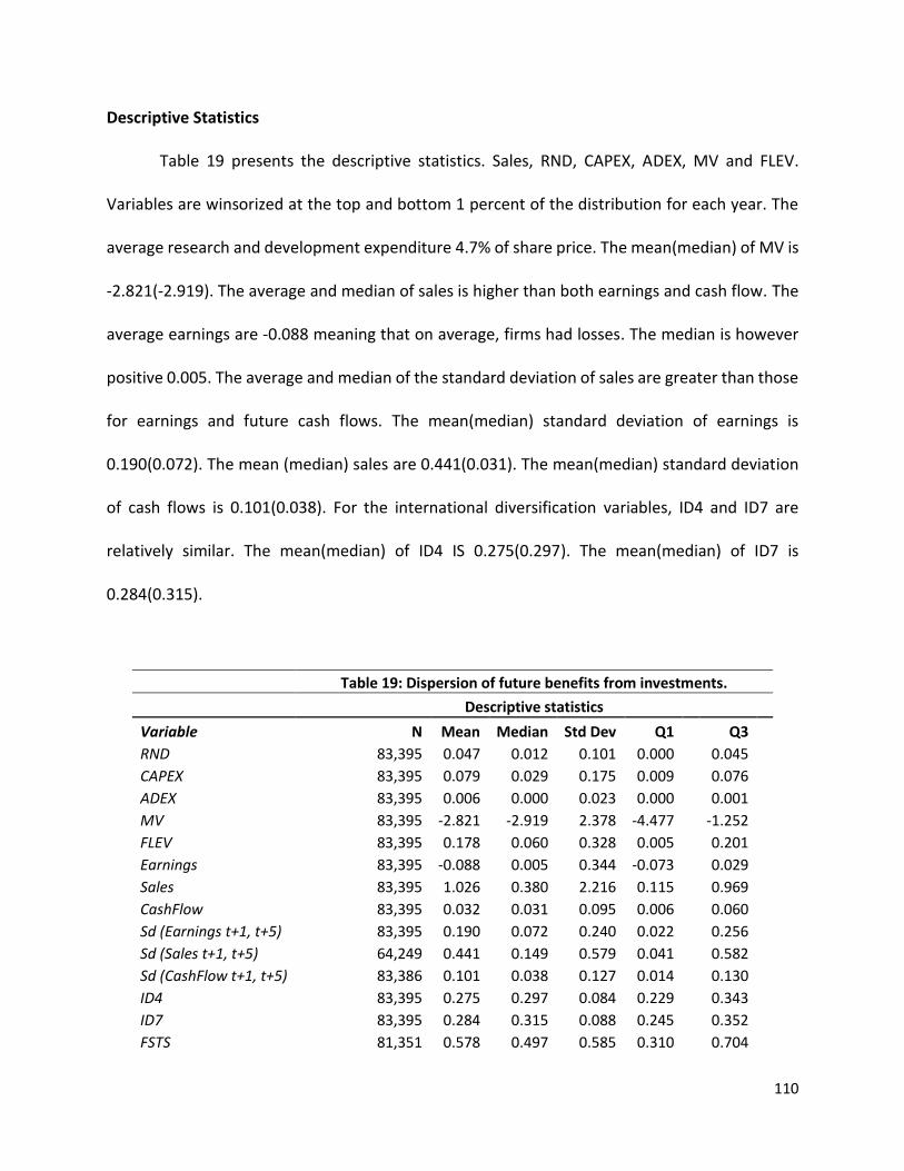
110
Descriptive Statistics
Table 19 presents the descriptive statistics. Sales, RND, CAPEX, ADEX, MV and FLEV.
Variables are winsorized at the top and bottom 1 percent of the distribution for each year. The
average research and development expenditure 4.7% of share price. The mean(median) of MV is
-2.821(-2.919). The average and median of sales is higher than both earnings and cash flow. The
average earnings are -0.088 meaning that on average, firms had losses. The median is however
positive 0.005. The average and median of the standard deviation of sales are greater than those
for earnings and future cash flows. The mean(median) standard deviation of earnings is
0.190(0.072). The mean (median) sales are 0.441(0.031). The mean(median) standard deviation
of cash flows is 0.101(0.038). For the international diversification variables, ID4 and ID7 are
relatively similar. The mean(median) of ID4 IS 0.275(0.297). The mean(median) of ID7 is
0.284(0.315).
Table 19: Dispersion of future benefits from investments.
Descriptive statistics
Variable N Mean Median Std Dev Q1 Q3
RND 83,395 0.047 0.012 0.101 0.000 0.045
CAPEX 83,395 0.079 0.029 0.175 0.009 0.076
ADEX 83,395 0.006 0.000 0.023 0.000 0.001
MV 83,395 -2.821 -2.919 2.378 -4.477 -1.252
FLEV 83,395 0.178 0.060 0.328 0.005 0.201
Earnings 83,395 -0.088 0.005 0.344 -0.073 0.029
Sales 83,395 1.026 0.380 2.216 0.115 0.969
CashFlow 83,395 0.032 0.031 0.095 0.006 0.060
Sd (Earnings t+1, t+5) 83,395 0.190 0.072 0.240 0.022 0.256
Sd (Sales t+1, t+5) 64,249 0.441 0.149 0.579 0.041 0.582
Sd (CashFlow t+1, t+5) 83,386 0.101 0.038 0.127 0.014 0.130
ID4 83,395 0.275 0.297 0.084 0.229 0.343
ID7 83,395 0.284 0.315 0.088 0.245 0.352
FSTS 81,351 0.578 0.497 0.585 0.310 0.704

111
5.4.2 Effect of international Diversification on the relation between R&D investments and
earnings variability
Table 20 presents the results for the analysis of the effects of international diversification
on the relation between research and development investments and dispersion of earnings. The
coefficient of ID is positive and significant at the 1 percent level in all three cases. The coefficients
of ID1, ID7 and FSTS are 0.014, 0.018 AND 0.02 respectively. They are all significant at the 1
precent level. The coefficient of the coefficient of RND is positive and significant in all columns.
The positive and significant coefficients shows that RND is positively related to the dispersion of
earnings. This is consistent with prior literature that finds that there is greater uncertainty with
future benefits from investments in research and development. The higher uncertainty is
captured by the dispersion of operating income. The interaction of RND and ID captures the
effect of international diversification on the relation between RND and dispersion of operating
income. For all three regressions, the coefficient of the interaction between research and
development and international diversification (RND*ID) is negative and significant at the 1
percent level. The t-values range from -2.33 in the case of FSTS to -3.19 for ID7.
Hypothesis 4 predicts that international diversification is negatively associated with
uncertainty with dispersion of future benefits from R&D investments. In other words,
international diversification reduces the positive association between R&D and earnings
variability. The negative coefficients of RND*ID are consistent with this prediction. For all the
three proxies of international diversification, ID reduces future earnings variability.
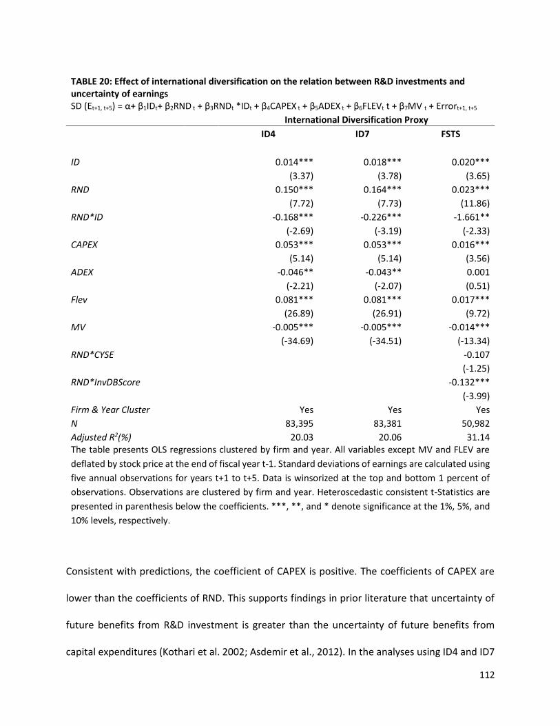
112
TABLE 20: Effect of international diversification on the relation between R&D investments and uncertainty of earnings SD (Et+1, t+5) = α+ β1IDt+ β2RND t + β3RNDt *IDt + β4CAPEX t + β5ADEX t + β6FLEVt t + β7MV t + Errort+1, t+5
International Diversification Proxy
ID4 ID7 FSTS
ID 0.014*** 0.018*** 0.020***
(3.37) (3.78) (3.65)
RND 0.150*** 0.164*** 0.023***
(7.72) (7.73) (11.86)
RND*ID -0.168*** -0.226*** -1.661**
(-2.69) (-3.19) (-2.33)
CAPEX 0.053*** 0.053*** 0.016***
(5.14) (5.14) (3.56)
ADEX -0.046** -0.043** 0.001
(-2.21) (-2.07) (0.51)
Flev 0.081*** 0.081*** 0.017***
(26.89) (26.91) (9.72)
MV -0.005*** -0.005*** -0.014***
(-34.69) (-34.51) (-13.34)
RND*CYSE -0.107
(-1.25)
RND*InvDBScore -0.132***
(-3.99)
Firm & Year Cluster Yes Yes Yes
N 83,395 83,381 50,982
Adjusted R2(%) 20.03 20.06 31.14 The table presents OLS regressions clustered by firm and year. All variables except MV and FLEV are
deflated by stock price at the end of fiscal year t-1. Standard deviations of earnings are calculated using
five annual observations for years t+1 to t+5. Data is winsorized at the top and bottom 1 percent of
observations. Observations are clustered by firm and year. Heteroscedastic consistent t-Statistics are
presented in parenthesis below the coefficients. ***, **, and * denote significance at the 1%, 5%, and
10% levels, respectively.
Consistent with predictions, the coefficient of CAPEX is positive. The coefficients of CAPEX are
lower than the coefficients of RND. This supports findings in prior literature that uncertainty of
future benefits from R&D investment is greater than the uncertainty of future benefits from
capital expenditures (Kothari et al. 2002; Asdemir et al., 2012). In the analyses using ID4 and ID7
113
as proxies for international diversification, the coefficient of ADEX is negative and significant. This
is contrary to predictions, and some of the findings in prior literature (Asdemir et al. 2012).
However, most of the firms did not report advertising expenses.
Appendix 10 presents results of alternative tests, without CYSE and InvDBScore in the
regressions using FSTS as the proxy for international diversification. Consistent with the main
analyses, the coefficient of interaction between FSTS and RND is negative and significant at the
one percent level.
5.4.3 Effect of international Diversification on the relation between R&D investments and cash
flow variability
The results for the examination of the effects of international diversification on the
relation between R&D investments and variability of future cash flows are presented in table 21.
The coefficient of ID is positive and significant at the 1 percent level in all three analyses. The
coefficient of ID4(ID7) IS -0.039(0.051) with a t-value of 3.59(3.65). The coefficient of FSTS is -
0.014 with the t-value of -0.10. In all three cases, the coefficient of RND is positive and significant
at the one percent level. For ID4(ID7), the coefficient of RND is 0.36 (0.38). The positive and
significant coefficients shows that RND is associated with greater cash flow dispersion. These
results are in line with prior literature that finds that there is greater uncertainty with future
benefits from investments in research and development.
The interaction of RND and ID captures the effect of international diversification on the
relation between RND and the uncertainty of cashflow. Hypothesis 4 predicts that international
diversification reduces the degree of variability of future benefits from investment in R&D. That

114
is H4: β3<0. For all three regressions, the coefficients of the interaction between research and
development and international diversification (RND*ID) are negative and significant. The
coefficient of interaction between RND and both ID4 and FSTS are significant at the 1 percent
level. Hypothesis 4 predicts that international diversification is negatively associated with
uncertainty with dispersion of future benefits from R&D investments. That is international
diversification, reduces the positive association between R&D and earnings variability. The
negative coefficient of RND*ID is consistent with this prediction. For all the three proxies of
international diversification, ID reduces cash-flow variability. As predicted, the coefficient of
CAPEX is positive. The coefficient of ADEX is positive and significant. This is consistent with to
predictions and findings in prior research (Asdemir et al. 2012).
To compare results between ID4, ID7 and FSTS, I rerun the FSTS regression without CYSE
and InvDBScore. The results are presented in appendix 10. The resulting coefficient FSTS is
positive and significant at the 1 percent level. The coefficient of interaction between FSTS and ID
is negative and significant at the one percent level. This lends further support for hypothesis 4.
However, the coefficient of ADEX is positive and significant which is contrary to the expectations.

115
TABLE 21: Effect of international diversification on the relation between R&D investments and uncertainty of cash flow from operations
SD (CFt+1, t+5) = α+ β1IDt+ β2RND t+ β3RNDt *IDt + β4CAPEX t + β5ADEX t + β6FLEVt t + β7MV t + Errort+1, t+5
International Diversification Proxy
ID4 ID7 FSTS
ID 0.039*** 0.051*** -0.014
(3.59) (3.65) (-0.1)
RND 0.361*** 0.382*** 0.009***
(14.4) (6.63) (14.22)
RND*ID -0.237*** -0.322* -6.485***
(-2.91) (-1.68) (-3.14)
CAPEX 0.407*** 0.407*** 0.006***
(32.55) (12.97) (4.18)
ADEX 0.316*** 0.318*** 0.015***
(8.46) (4.17) (3.13)
Flev 0.371*** 0.371*** 0.002***
(108.8) (40.8) (6.32)
MV -0.017*** -0.017*** -0.004***
(-42.72) (-39.21) (-14.09)
RND*CYSE 0.030
(1.05)
RND*InvDBScore -0.044***
(-3.93)
Firm & Year Cluster Yes Yes Yes
N 83,386 83,372 50,982
Adjusted R2(%) 30.49 30.5 44.47 The table presents OLS regressions clustered by firm and year. All variables except MV and FLEV are
deflated by stock price at the end of fiscal year t-1. Standard deviations of cashflow from operations
are calculated using five annual observations for years t+1 to t+5. Data is winsorized at the top and
bottom 1 percent of observations. Observations are clustered by firm and year. Heteroscedastic
consistent t-Statistics are presented in parenthesis below the coefficients. ***, **, and * denote
significance at the 1%, 5%, and 10% levels, respectively.

116
5.4.3. Effect of international Diversification on the relation between R&D investments and
variability in sales revenue
Table 22 presents the results for the variability in sales. The coefficients of RND in both
the ID4 and ID7 analyses are not significant. Further, the interaction between investment in
research and development and international diversification is not significant in the ID4 and ID7
analyses. Therefore, the results do not support a significant relation between ID4 and ID7 and
dispersion of future sales revenue. The insignificant results for ID4 and ID7 do not offer support
to the prediction that international diversification reduces future earnings variability in the case
of sales revenue. In the analysis with FSTS as the proxy for international diversification, the
coefficient of RND is positive and significant at the 1 percent level. Further, the coefficient of
interaction between FSTS and ID is negative and significant at the 1 percent level. This result lends
support to hypothesis H4.
Considering the control variables, the coefficient of CAPEX is positive and significant. The
coefficient of ADEX is positive and significant in the FSTS analysis. It is insignificant in the analyses
using ID4 and ID4 as the proxies for international diversification. The coefficient of MV is
negatively significant in the first two columns. For ID4 and ID7, the coefficient of MV is small and
significant at a 5 percent level.
In an additional test, I rerun the FSTS analysis without CYSE and InvDBScore in the model.
The result is presented in Appendix 10. Consistent with predictions in H4, I find that the
coefficient of R& D is positive and significant in the regression with FSTS as the proxy for
international diversification. In the third column the coefficient of interaction between FSTS and

117
RND is negative and significant at the 1 percent level. This supports the prediction that
international diversification reduces the variability of sales revenue benefits from R&D
investments.
TABLE 22: Effects of international diversification on the relation between R&D investments and sales revenue variability
Model: SD (St+1, t+5) = α+ β1ID t + β2RND+ β3RND *ID + β4ADEX t + β5FLEV t + β6MV t + Errort+1, t+5
International Diversification Proxy
ID4 ID7 FSTS
ID -0.014 -0.014 0.005
(-1.24) (-1.28) (0.08)
RND 0.042 0.039 0.036***
(0.53) (0.53) (8.4)
RND*ID 0.353 0.368 -1.723***
(1.34) (1.46) (-2.91)
CAPEX 0.354*** 0.355*** 0.079***
(9.77) (9.89) (9.07)
ADEX 0.000 -0.001 0.000***
(-0.01) (-0.04) (5.04)
Flev 0.004 0.004 0.005***
(0.98) (1.01) (17.61)
MV -0.000** -0.000** -0.001***
(-2.39) (-2.33) (-11.46)
RND*CYSE 0.096***
(3.98)
RND*InvDBScore -0.020***
(-3.91)
Firm & Year Cluster Yes Yes Yes
N 61,222 61,222 50,982
Adjusted R2(%) 16.87 16.88 17.29 The table presents OLS regressions clustered by firm and year. All variables except MV and FLEV are
deflated by stock price at the end of fiscal year t-1. Standard deviations of sales revenue are calculated
using five annual observations for years t+1 to t+5. Data is winsorized at the top and bottom 1 percent
of observations. Observations are clustered by firm and year. Heteroscedastic consistent t-Statistics are
presented in parenthesis below the coefficients. ***, **, and * denote significance at the 1%, 5%, and
10% levels, respectively.
118
CHAPTER 6. CONCLUSION
6.1 Motivation
This dissertation focuses on the relationship between international diversification and
two main aspects: cost rigidity and investment characteristics. The focus on international
diversification motivated by several reasons. First, international diversification is increasingly
important as it plays a pivotal role in firms’ strategic behavior (Hitt et al.,1996) and firm
competitiveness (Franko, 1989). Secondly, international diversification presents unique benefits,
challenges, and costs to firms (Caves 1989; Lu and Beamish, 2004). Thirdly, there is evidence of
increases in international diversification despite documented failures to realize expected
performance (McGee 2014; Weber et al.,2013). Finally, prior literature has voids, coupled with
inconsistent findings and puzzles (Shimizu et al., 2004).
Prior studies find mixed relationship regarding the nature of the performance in
international diversification. Prior literature examining performance in international diversified
firms document various patterns of performance. Some find a linear relation (e.g., Tallman and
Li, 1996), some find a U-Curve (e.g., Lu and Beamish, 2001); inverted U-curve (Hitt et al., 1997),
and horizontal S-Curve (Lu and Beamish, 2004). The mixed results and evidence that firms face
greater challenges as they increase their diversification levels beyond optimal levels, suggest
non-linear relationships. In part of the analyses, I therefore, separate firms into those with low
to medium levels of international diversification and those with higher levels of diversification.
I examine two main research questions. The first question is whether international
diversification is related to cost rigidity. This research question is motivated by the scarcity of
evidence examining the link between internationalization and changes in cost behavior and
119
characteristics. Banker et al. (2014) finds a positive relationship between demand uncertainty
and cost rigidity. They find that as uncertainty increases, there are decreases in the degree of
change in costs in response to changes in sales revenue. Uncertainty is one of the main factors
that firms diversifying internationally face.
The second question is whether international diversification affects investment
characteristics. Thou there is a large body of research examining international diversification and
investment characteristics, there is a scarcity of literature examining the link between the two.
In this research, I examine three investment characteristics: investment efficiency, uncertainty of
future benefits from investments and research and development intensity. Prior studies have
investigated these investment characteristics. Biddle et al. (2009) finds a positive association
between financial reporting quality and investment efficiency. Based on a sample of
multinational corporations, Amberger et al (2021), find evidence that repatriation taxes reduce
subsidiary-level investment efficiency. They find that the effect is higher for subsidiaries that have
high information asymmetry and weak monitoring. Unlike, Amberger et al., (2021), my research
focuses on the overall (parent) firm investment- efficiency, not just the subsidiaries.
Investments in research and development and innovation has received significant
attention in prior literature. For instance, there are arguments in prior literature that process,
and product innovation are crucial to gaining competitive advantage in international markets
(Porter, 1991; Hitt et al., 1997). International diversification improves technological learning and
fosters innovation (Zahra et al., 2000), and it facilitates appropriation of innovations (Kotabe,
1990). Despite the greater opportunity for innovation in international markets, there is evidence
that firms may make tradeoffs between various corporate strategies (Hoskisson and Hitt, 1990;
120
Geringer et al., 1989). Banker et al. (2011) finds that firms with a higher degree of diversification
are likely to innovate through acquisitions, instead of investing in R&D. These findings and the
pivotal nature of international diversification provides motivation into my examining the link
between international diversification and R&D intensity. Hitt et al., (1997) find evidence that
international diversification is positively related to R&D intensity. However, their sample was
restricted to only three years. Except for Hitt et al. (1997). I am not aware of any other study that
examines the relation between international diversification and R&D intensity.
Kothari et al. (2002) finds that relative to investments to property, plant and equipment,
investments in R&D generate future benefits that are more uncertain. Amir et al. (2007) finds that relative
to capital investments, R&D investments lead to greater earnings variability only in R&D intensive
industries. Asdemir et al. (2012) find that compared to capital expenditures, R&D expenditures generate
significantly less uncertain future benefits when it comes to sales revenue. Further, their findings were
inconclusive regarding operating cashflows. The inconsistency in these prior studies warrants further
examination. The unique challenges and opportunities faced by multinational companies provides an
opportunity to examine how international diversification affects the uncertainty of future benefits from
R&D investments.
6.2 Hypotheses, Findings, and Discussions
Regarding my first research question, I investigate the association between international
diversification and cost rigidity. Cost rigidity is the short-run change in cost in response to a
change in sales revenue. I examine three cost categories, SG&A costs, cost of goods sold and the
number of employees. I hypothesize that that for firms with low to medium levels of international
diversification, international diversification is negatively associated with cost rigidity(H1a).

121
Secondly, I hypothesize that for firms with higher levels of international diversification,
international diversification is positively related to cost rigidity(H1b). I follow the approach in
Banker et al. (2014) in testing the hypotheses.
In tests for H1a, I run the analyses on the sample of firms with low to medium levels of
international diversification. From the results for SG&A, COGS, and the number of employees for
the first two proxies of international diversification ID4 and ID7 are consistent with predictions.
Thus, I find support for hypothesis 1a. In tests using FSTS, together with country scope and the
inverse of doing-business scores, I find the expected result for SGA only. In additional analyses, I
rerun tests using FSTS only (without country scope and the inverse of the doing-business score).
The result for FSTS in the additional analyses offers support for hypothesis 1a in the case of COGS.
Similar to the main analyses, the FSTS remains insignificant for the analyses using the number of
employees. In sum, for the sample of firms with low to medium levels of international
diversification the results are mostly consistent with hypothesis 1a. That is at low to medium
levels of international diversification, there is a negative relation between international
diversification and cost rigidity
These results are attributable to several reasons that have been documented in prior
literature. For instance, prior literature has found that firms prioritize familiar markets (e.g.,
Davidson, 1983) and companies limit fixed costs when they expand to familiar markets (Hisey
and Caves, 1985). Familiar markets enable appropriations of home country competencies and
cost reductions (Gomes and Ramaswamy, 1999). Cost reductions can result from activity sharing
which may lead to decreases in overall fixed costs and cost rigidity. As firms expand globally, they
pursue and attain various synergistic gains and economies of scale (Larsson and Finkelstein).
122
Firms with low to moderate levels of international diversifications can benefit more from the
advantages and synergistic gains from expanding to markets that are geographically more
accessible and have greater similarities with the domestic markets. Greater sharing of lumpy
assets and resources leads to lower fixed costs, hence an overall decrease in cost rigidity.
To test hypothesis 1b, I run regressions using the subsample of firms with higher levels of
diversification. On the overall, the results for firms with higher levels of international
diversification are mixed. In the main analyses, I find consistent evidence in support of hypothesis
1b in the case of SGA. For employees, I find support for hypothesis 1b in the ID4 and ID7 analyses.
In the results for SG&A and COGS, the results from using FSTS as the proxy for international
diversification are as predicted in the main analyses. However, additional analysis using FSTS and
excluding CYSE and InvDBScore from the model fail to offer support for H1b. The result for COGS
is mostly inconsistent with predictions in hypothesis 1b. That is, the evidence fails to support the
prediction that firms with higher levels of international diversification changes in COGS will be
more rigid given a given level of change in sales revenue.
The increased rigidity for SG&A costs and the number of employees can result from
various factors highlighted in prior studies. For instance, there are arguments that greater
dispersion leads to greater coordination and communication barriers Porter (1990; Hitt et al.,
1997). These barriers are likely to affect sharing fixed resources. For instance, communication
barriers may encourage establishment of more foreign administrative offices. Such actions lead
to increases in fixed asset investments and the corresponding costs. There are arguments in prior
literature that as firms expand globally are likely to encounter increased need for higher fixed
123
costs due to factors such as increasing difficulty of sharing fixed assets due to physical, political,
and other barriers as firms expand into more regions.
I find minimal evidence of positive association between international diversification and
cost rigidity in the case of COGS. The fact that hypothesis 1b is not supported for COGS, suggest
that firms at higher levels of international diversification are better adapted and able to respond
quickly to changes in demand. Such firms have greater resources and are in position to take
advantage of their resources and share fixed assets such as factories and machinery. For instance,
their financial and other resources enable them to have well developed supply chains and
transportation systems. The changes in the past decades have led to lower coordination,
communication, and other costs that facilitate resource and activity sharing. Consequently, there
is increased mobility of raw materials across a company’s operational areas. Further, an increase
in globalization and ease with which products are moved across the globe, plays a critical role in
activity and resource sharing. Greater sharing of fixed resources related to production leads to
decreases in cost rigidity.
The findings above have several implications. First, the negative association between ID
and cost rigidity for firms at low to medium levels of international diversification means that
these firms are benefiting from sharing fixed assets and activities. This is important for managers
and firms as international diversification is an important strategic avenue. Resource-based view
highlights the various resource advantages that firms gain as they expand. The findings for the
firms in low to medium levels of international diversification are consistent with arguments from
the resource-based view. Secondly, the evidence of higher cost rigidity for SG&A costs and
number of employees for firms with higher levels of international diversification, has implications

124
for managers and companies. The results suggest that firms may be better off if they restrict their
global expansion to a certain optimum level. The optimum level varies with the firms due to
factors such as experience, strategic location choices, and so forth. Investors may therefore wish
to incorporate the level of international diversification as one of their company evaluation
factors.
Regarding optimal investment, underinvestment and overinvestment are both an
indication of investment inefficiency. I examine the relation between international diversification
and both under and over investment. I perform conditional and unconditional tests separately
for each subsample of firms. For the subsample of firms with low to medium levels of
international diversification, I predict that international diversification is negatively associated
with both underinvestment and overinvestment. In the conditional tests I find limited support of
investment in settings where firms are prone to underinvest. For all three analyses, I find
evidence of significant negative association between international diversification and
overinvestment.
In the unconditional tests, the results support hypothesis 2a and 2b. That is, I find
significant negative associated between international diversification and under investment. For
overinvestment, the results fail to offer support for the predicted negative association between
international diversification and overinvestment. On the overall, the analyses for the firms with
low to medium levels of international diversification offer some evidence of greater investment
efficiency, especially regarding underinvestment. The results offer support to the hypothesis and
suggests that these firms experience reductions in suboptimal investments as their levels of
international diversifications increase. This is consistent with resource-based theory ((Penrose,

125
1959; Barney, 1991) whereby firms are taking advantage of bundles of resources. International
diversification facilitates acquisitions and value creation from resources as firms get more
opportunities to appropriate their knowledge, skills, and other resources (Amit and Schoemaker,
1993). These opportunities include factors that promote optimal investment.
In the examination of the subsample of firms with higher levels of international
diversification, I predict that international diversification is positively associated with both under-
investment (H2d) and over-investment (H2c). In the unconditional tests, I find some evidence
supporting both hypothesis 2c and 2d. For two out of the three proxies for international
diversification, I find positive association between international diversification and both under-
investment and over-investment. FSTS is insignificant and it does not offer support for the
predictions. The results from the unconditional tests provide evidence of a positive association
between international diversification and both over-investment and under-investment. The
results from the analyses using the sample of firms with higher levels of international
diversification suggest that these firms have greater suboptimal investment as evidenced by
greater under-investment and over-investment. Some of the possible causes of suboptimal
investment choices can be the increasing uncertainties, complexities, and information processing
costs that firms face in foreign markets (Child et al., 2001). The effects of complexity may be
worsened by the considerable number of investment options that are available in foreign
markets, coupled with greater information asymmetries and barriers.
The findings above have implications for various stakeholders. For managers and
companies, evidence of negative association between international diversification and both
under- and over- investment at low to medium levels of international diversification suggest that

126
firms can have better investment outcomes if they operate within lower to medium levels of
international diversification. Investors can incorporate this knowledge in evaluating firms that
they can potentially invest in.
In the R&D intensity analyses, I predict the existence of a relationship. I, however, do not
predict a specific direction regarding the relationship between international diversification and
R&D investments. The reason for not having a specific direction is that, as firms diversify
internationally, they face two sets of factors. Those that promote investment in R&D and those
that decrease the need for R&D investments. Factors such as the need for unique products to
meet customer preferences in foreign market encourage R&D investment. On the other hand,
firms diversifying internationally can gain innovation and competencies by acquiring other firms.
Acquisition of firms fulfils some of the research and development investment as acquired firms
have specialized knowledge that the acquirer can appropriate.
From the findings for both the fixed effects and OLS regressions, international
diversification is positively related to research and development intensity. The significant findings
lend support to hypothesis 3. Further analysis shows that the positive relationship is limited to
low to medium levels of international diversification.
The last research question I examine is the relationship between international
diversification and uncertainty of future benefit from investments in R&D. I hypothesize that
international diversification reduces the variability of future benefits from investments in R&D
(Hypothesis 4). I use three proxies of future benefits from investment: operating income,
operating cash flows, and sales revenues. Results from the analysis of dispersion of earnings
variability support my predictions. The findings from all the three proxies for international

127
diversification support the hypothesis. In the analyses of variability of future cash flows, I find
evidence in support of the prediction that international diversification reduces the variability in
future cash flows. In the analyses of variability of sales revenue, the results do not support the
predictions. This is contrary to the findings in prior literature (e.g., Amir et al., 2007). These
findings contribute to the body of literature examining variability in earnings and other
performance variables.
The findings of negative association between international diversification and earnings
variability have various implications for managers, companies, and investors. The evidence in
support of decreased earnings variability in the case of earnings and cash flows suggests that
international diversification can help mitigate some of the uncertainties in both the domestic and
other foreign markets. For investors, the findings highlight the potential to reduced personal
financial risks by investing in firms that are internationally diversified.
6.3. Limitations and Recommendations
There are various limitations in this research. The first limitation relates to the proxies for
international diversification. The use of ID4 and ID7 as proxies for international diversification
has various limitations. For instance, there is use of segment data which is incomplete and suffers
from lack of uniformity in the nature and the aggregation of sales information. For instance,
aggregated regional data vary by companies and some do not directly fit into regions defined in
Hitt et al. (1997) and the World Bank reports. FSTS suffers from limitations. First, data on foreign
sales is incomplete and inconsistent. Secondly, FSTS only measures the ratio of foreign sales
without capturing other factors that businesses face in the global environment. For instance,
128
legal, economic, and cultural aspects that lead to higher coordination, communication, resource
sharing, and other costs. Significant results from the inclusion of country scope and proxy for the
difficulty of doing business in a country or region highlight that these factors are important.
Similarly, the usage the inverse of the average of doing-business scores has shortcomings
because of lack of data on the accurate weights of each country or region. The lack of accurate
weights stem from data aggregation issues in the available segment data. The limitations with
the FSTS measure are evident from the results showing that its effect is inconsistent in some of
the analyses.
A possible modification to address the shortcomings of proxies for international
diversification is to create a composite measure that combines the region complexity and the
proportion of the sales. An in-depth examination of firm data can help mitigate errors and
promote better weighting and inclusion of the relevant factors. However, the limitation in the
available data necessitates significant hand-collected data to increase information reliability.
Another limitation relates to other sample and data availability issues. In the investment
efficiency analyses, there is limited data for corporate governance variables. For instance, G-
Index (Gompers et al., 2003), is only available for 1990 to 2006. In future, I could extend this
examination by finding alternative governance variables that have data spanning more years.
Econometric issues related to sample selection and sample characteristics present
another limitation. For instance, whether a company is internationally diversified is not random.
Firms with certain observable and unobservable characteristics will tend to diversify
internationally. Similarly, the availability of firm specific data is not always random. For example,
larger firms may tend to have more complete information. This is because larger firms have
129
greater financial and knowledges resources that can be devoted to collection and analysis of
relevant information including segment data, among others. Some of the results may therefore
be biased by unobserved factors. The use of fixed-effects models in this research mitigates some
of the unobservable factors. Another potential way of addressing this short coming would be to
have control samples of firms with similar characteristics.
There are several areas that this research can be extended. The examination of cost
rigidity can be expanded to determine if the results hold if cost and revenue patterns in prior
years are incorporated in the analyses. A reexamination of the cost analyses for specific sample
of countries can help inform whether firms are adapting to global imbalances in labor and
production factors. For instance, an examination of companies with operations in developing
countries can illuminate if cheap labor plays a critical role in the strategic decisions, and if it has
significant effect on firm outcomes. In the case of investment efficiency, the study can be fine-
tuned to examine specific countries and subsidiary characteristics. For example, the examination
of whether the characteristics of the country culture or subsidiary’s management affect
investment efficiencies.
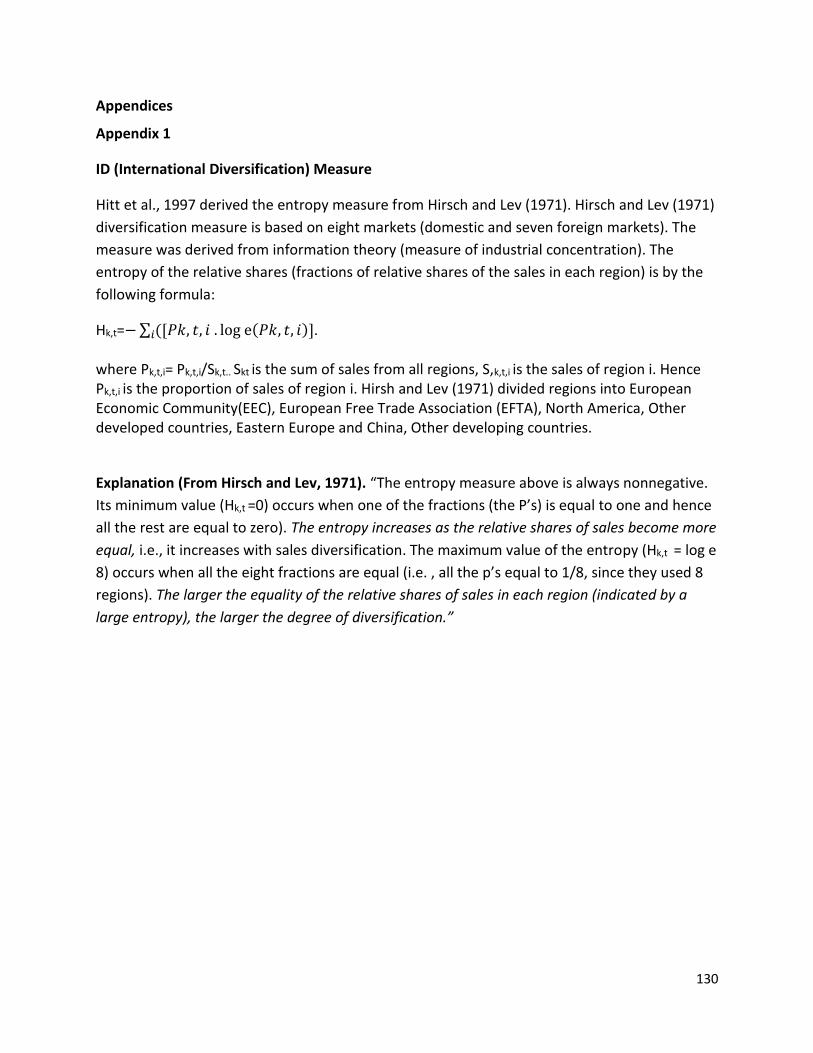
130
Appendices
Appendix 1
ID (International Diversification) Measure
Hitt et al., 1997 derived the entropy measure from Hirsch and Lev (1971). Hirsch and Lev (1971)
diversification measure is based on eight markets (domestic and seven foreign markets). The
measure was derived from information theory (measure of industrial concentration). The
entropy of the relative shares (fractions of relative shares of the sales in each region) is by the
following formula:
Hk,t=− ∑ ([𝑃𝑘, 𝑡, 𝑖 . log e(𝑃𝑘, 𝑡, 𝑖)]𝑖 . where Pk,t,i= Pk,t,i/Sk,t.. Skt is the sum of sales from all regions, S,k,t,i is the sales of region i. Hence Pk,t,i is the proportion of sales of region i. Hirsh and Lev (1971) divided regions into European Economic Community(EEC), European Free Trade Association (EFTA), North America, Other developed countries, Eastern Europe and China, Other developing countries.
Explanation (From Hirsch and Lev, 1971). “The entropy measure above is always nonnegative.
Its minimum value (Hk,t =0) occurs when one of the fractions (the P’s) is equal to one and hence
all the rest are equal to zero). The entropy increases as the relative shares of sales become more
equal, i.e., it increases with sales diversification. The maximum value of the entropy (Hk,t = log e
8) occurs when all the eight fractions are equal (i.e. , all the p’s equal to 1/8, since they used 8
regions). The larger the equality of the relative shares of sales in each region (indicated by a
large entropy), the larger the degree of diversification.”

131
51Illustration of Hitt et al. (1997) ID scores:
Region 1 Region 2 Region 3 Region 4
Firm 1 Total Sales ID Score
Region Sales 10.000 20.000 30.000 40.000 100.000
Pi 0.100 0.200 0.300 0.400 1.000
Pi*ln(1/pi) 0.230 0.322 0.361 0.367 1.280 1.280
Firm 2 Region Sales 25.000 25.000 50.000 0.000 100.000
Pi*ln(1/pi) 0.250 0.250 0.500 0.000 1.000 0.347 0.347 0.347 0.000 1.040 1.040
Firm 3 0.000 50.000 50.000 0.000 100.000
Region Sales 0.000 0.500 0.500 0.000 1.000 Pi*ln(1/pi) 0.000 0.347 0.347 0.000 0.693 0.693
Firm 4 100.000 0.000 0.000 0.000 100.000
Region Sales 1.000 0.000 0.000 0.000 1.000
Pi*ln(1/pi) 0.000 0.000 0.000 0.000 0.000 0.000
Firm 5 0.000 10.000 40.000 50.000 100.000
Region Sales 0.000 0.100 0.400 0.500 1.000
Pi*ln(1/pi) 0.000 0.230 0.367 0.347 0.943 0.943
Firm 6 Total Sales ID Score
Region Sales 25.000 25.000 25.000 25.000 100.000
Pi 0.250 0.250 0.250 0.250 1.000
Pi*ln(1/pi) 0.347 0.347 0.347 0.347 1.386 1.386
51 Miller and Pras, 1980 uses approach similar to Hirsh and Lev’s – with number of firm holdings
or number of subsidiaries instead of sales.

132
Appendix 2. Variables Definitions
International diversification:
• ID-International diversification measure.
• ID4 and ID7=ID4 and ID7 are empirical proxies for international diversification, computed as
ID=∑ ([𝑃𝑖 . ln (1
𝑃𝑖)]𝑖 For all observations of firm i. Where Pi is the sales attributed to the
global market region i and Ln (1/Pi) is the weight given to each global market region or the natural logarithm of the inverse of its sales. For ID4, the four regions are Africa, Asia and Pacific, Europe, and the Americas. For ID7, the regions are East Asia and Pacific, Europe and Central Asia, Latin America and Caribbean, Middle East and North Africa, North America, South Asia, and Sub-Saharan Africa. Further details and illustration for computing ID4 and ID7 are provided in appendix 1.
• FSTS (Foreign Sales to total sales) = ratio of foreign sales to total sales
• FSTS_dc=A linear combination of FSTS, InvDBScore and CYSE. It is computed using the Estimate command in SAS.
• CYSE = country scope; the number of countries in which a firm has foreign operations.
• InvDBscore= 100 minus firm i’s average doing business score. Doing business scores are obtained from World Bank Reports. The scores capture the ease of doing business in each country or region. The score includes trading across border measures as well as other measures that affect business within a country or region. The doing-business scores ranges from 0 to 100, such that countries with the greatest ease of doing business have a score of 100. Therefore, countries that have lower ease of doing business have higher InvDBscores. Cost rigidity:
• ΔLnSALESi,t=Log-change in deflated sales of firm i from year t-1 to year t.
• GDP_Growth=GDP growth in year t.
• Ind_Code=Four-digit industry dummies based on Fama and French 48 industry classifications.
• ΔLnSGA=Log-change in deflated SG&A costs of firm i from year t-1 to year t.
• ΔLnCOGS=Log-change in deflated cost of goods sold of firm i from year t-1 to year t.
• ΔLnEMP=Log-change in the number of employees of firm i from year t-1 to year t.
• Cost=operating costs, either Selling General and Administrative Costs (SGA); Cost of Goods Sold (COGS) and Number of employees (EMP).
• Sales=total sales revenue Investment characteristics:
• Investment =the sum of research and development expenditure, capital expenditure, and acquisition expenditure less cash receipts from sale of property, plant, and equipment multiplied by 100 and scaled by lagged total assets.

133
• LogAsset =the log of total assets.
• Mkt-to-Book=the ratio of the market value of total assets to book value of total assets
• CFO= cash flow from operations.
• Sales=total sales revenue.
• Z-Score=A measure of distress computed following the methodology in Altman (1968). =3.3(item 170) +(item 12) +0.25(item 36) +0.5((items 4−item 5)/item 6)52.
• Tangibility=the ratio of PPE (property, plant, and equipment) to total assets.
• K-structure=the ratio of long-term debt to the sum of long-term debt to the market value of equity
• Ind. K-structure =mean K-structure for firms in the same SIC 3-digit industry.
• CFOsale=the ratio of CFO to sales
• Slack the ratio of cash to PPE
• Dividend=an indicator variable that takes the value of one if the firm paid a dividend.
• Age=the difference between the first year when the firm appears in CRSP and the current year.
• Loss=an indicator variable that takes the value of one if net income before extraordinary items is negative, and zero otherwise.
• RNDI= RNDI is measured as R&D expenses/number of employees (Hitt et al.,1997; Hill and Snell, 1988).
• Debt=Ratio of debt to the total of debt and owners’ equity.
• Subs=Subs is the total number of firm subsidiaries that a firm has in year t.
• RND is the current investment in R&D deflated by lagged market value of equity.
• ADEX= advertising expenditure deflated by market value of equity.
• FLEV= is the book value of debt divided by the sum of debt and market value of equity at the end of fiscal year t SIZE is firm size measured as total assets.
• SD (FVt+1, t+5) =the standard deviation of future benefits. The proxies for FV are sales revenue, earnings before depreciation, amortization, advertising and R&D, or operating cash flows
• CAPEX = the current investments in fixed capital deflated by lagged market value of equity.
• MV= the natural logarithm of the product of share price and common shares outstanding. PRC= price per share Governance characteristics:
• Institutions=the percentage of firm shares held by institutional investors.
• Analysts=the number of analysts following the firm.
• InvGscore= the measure of anti-takeover protection created by Gompers et al. (2003), multiplied by minus one.
• GscoreDummy=an indicator variable that takes the value of one if G-Score is missing and zero otherwise.
52 Compustat variable numbers
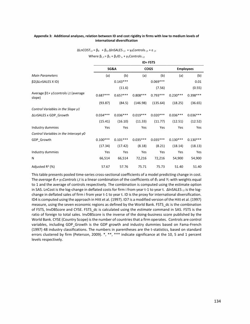
134
Appendix 3: Additional analyses, relation between ID and cost rigidity in firms with low to medium levels of international diversification
ΔLnCOSTi,t = β0 + βi,t ΔlnSALES i,t + γ0Controls i,t + ε i,t
Where βi, t = β1 + β2ID i, + γ1Controls i,t
ID= FSTS
SG&A COGS Employees
Main Parameters (a) (b) (a) (b) (a) (b)
β2(ΔLnSALES X ID) 0.143*** 0.069*** 0.01
(11.6) (7.56) (0.55)
Average β1+ γ1controls i,t (average slope)
0.687*** 0.657*** 0.808*** 0.793*** 0.230*** 0.398***
(93.87) (84.5) (146.98) (135.64) (18.25) (36.65)
Control Variables in the Slope γ1
ΔLnSALES x GDP_Growth 0.034*** 0.036*** 0.019*** 0.020*** 0.036*** 0.036***
(15.41) (16.10) (11.33) (11.77) (12.51) (12.52)
Industry dummies Yes Yes Yes Yes Yes Yes
Control Variables in the Intercept γ0
GDP_Growth 0.100*** 0.101*** 0.035*** 0.035*** 0.130*** 0.130***
(17.34) (17.42) (8.18) (8.21) (18.14) (18.13)
Industry dummies Yes Yes Yes Yes Yes Yes
N 66,514 66,514 72,216 72,216 54,900 54,900
Adjusted R2 (%)
57.67 57.76 75.71 75.73 51.40 51.40
This table presents pooled time-series cross-sectional coefficients of a model predicting change in cost. The average β1+ γ1Controls i,t is a linear combination of the coefficients of β1 and Y1 with weights equal to 1 and the average of controls respectively. The combination is computed using the estimate option in SAS. LnCost is the log-change in deflated costs for firm i from year t-1 to year t. ΔlnSALES i,t is the log-change in deflated sales of firm i from year t-1 to year t. ID is the proxy for international diversification. ID4 is computed using the approach in Hitt et al. (1997). ID7 is a modified version of the Hitt et al. (1997) measure, using the seven economic regions as defined by the World Bank. FSTS_dc is the combination of FSTS, InvDBScore and CYSE. FSTS_dc is calculated using the estimate command in SAS. FSTS is the ratio of foreign to total sales. InvDBScore is the inverse of the doing-business score published by the World Bank. CYSE (Country Scope) is the number of countries that a firm operates. Controls are control variables, including GDP_Growth is the GDP growth and industry dummies based on Fama-French (1997) 48 industry classifications. The numbers in parentheses are the t-statistics, based on standard errors clustered by firm (Peterson, 2009). *, **, *** indicate significance at the 10, 5 and 1 percent levels respectively.

135
Appendix 4: Additional analyses, relation between ID and cost rigidity in firms with higher levels of international diversification
ΔLnCOSTi,t = β0 + βi,t ΔlnSALES i,t + γ0controls i,t + ε i,t
Where βi, t = β1 + β2ID i, + γ1controls i,t
ID= FSTS
SG&A COGS Employees
Main Parameters (a) (b) (a) (b) (a) (b)
β2(ΔLnSALES X ID)
0.105***
-0.050***
0.046***
(13.78) (8.47) (3.98)
Average β1+ γ1controls i,t (average slope)
0.782*** 0.712*** 0.947*** 0.983*** 0.426*** 0.397***
(101.47) (77.32) (144.20) (125.56) (36.74) (29.25)
Control Variables in the Slope γ1
ΔLnSALES x GDP_Growth 0.027*** 0.027*** 0.030*** 0.030*** 0.062*** 0.062***
(12.39) (12.16) (17.11) (17.13) (22.34) (22.44)
Industry dummies Yes Yes Yes Yes Yes Yes
Control Variables in the Intercept γ0
GDP_Growth 0.086*** 0.084*** 0.051*** 0.051*** 0.195*** 0.195***
(15.51) (15.22) (11.37) (11.52) (26.27) (26.31)
Industry dummies Yes Yes Yes Yes Yes Yes
N 66,504 66,504 72,069 72,069 54893 54893
Adjusted R2 (%)
56.04 56.17 71.39 71.42 44.18 44.20
This table presents pooled time-series cross-sectional coefficients of a model predicting change in cost. The average β1+ γ1Controls i,t is a linear combination of the coefficients of β1 and Y1 with weights equal to 1 and the average of controls respectively. The combination is computed using the estimate option in SAS. LnCost is the log-change in deflated costs for firm i from year t-1 to year t. ΔlnSALES i,t is the log-change in deflated sales of firm i from year t-1 to year t. ID is the proxy for international diversification. ID4 is computed using the approach in Hitt et al. (1997). ID7 is a modified version of the Hitt et al. (1997) measure, using the seven economic regions as defined by the World Bank. FSTS_dc is the combination of FSTS, InvDBScore and CYSE. FSTS_dc is calculated using the estimate command in SAS. FSTS is the ratio of foreign to total sales. InvDBScore is the inverse of the doing-business score published by the World Bank. CYSE (Country Scope) is the number of countries that a firm operates. Controls are control variables, including GDP_Growth is the GDP growth and industry dummies based on Fama-French (1997) 48 industry classifications. The numbers in parentheses are the t-statistics, based on standard errors clustered by firm (Peterson, 2009). *, **, *** indicate significance at the 10, 5 and 1 percent levels respectively.
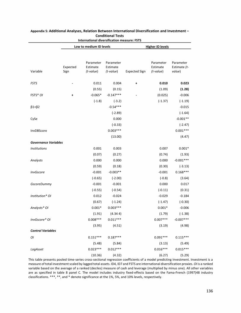
136
Appendix 5: Additional Analyses, Relation Between International Diversification and Investment – Conditional Tests
International diversification measure: FSTS
Low to medium ID levels Higher ID levels
Variable Expected Sign
Parameter Estimate (t-value)
Parameter Estimate (t-value) Expected Sign
Parameter Estimate (t-value)
Parameter Estimate (t-value)
FSTS - 0.011 0.004 + 0.010 0.023
(0.55) (0.15) (1.09) (1.28)
FSTS* OI + -0.065* -0.147*** - (0.025) -0.006
(-1.8) (-3.2) (-1.37) (-1.19)
β1+β2 -0.54*** -0.015
(-2.89) (-1.64)
CySe 0.000 -0.001**
(-0.33) (-2.47)
InvDBScore 0.003*** 0.001***
(13.00) (4.47)
Governance Variables
Institutions 0.001 0.003 0.007 0.001*
(0.07) (0.27) (0.74) (1.93)
Analysts 0.000 0.000 0.000 -0.001***
(0.59) (0.18) (0.30) (-3.13)
InvGscore -0.001 -0.003** -0.001 0.168***
(-0.65) (-2.00) (-0.8) (3.64)
GscoreDummy -0.001 -0.001 0.000 0.017
(-0.55) (-0.54) (-0.11) (0.31)
Institution* OI 0.012 -0.024 -0.029 -0.184
(0.67) (-1.24) (-1.47) (-0.30)
Analysts* OI 0.001* 0.003*** 0.001* -0.006
(1.91) (4.34 4) (1.79) (-1.38)
InvGscore* OI 0.008*** 0.011*** 0.007*** -0.007***
(3.95) (4.51) (3.19) (4.98)
Control Variables
OI 0.151*** 0.187*** 0.091*** 0.115***
(5.48) (5.84) (3.13) (5.49)
LogAsset 0.023*** 0.012*** 0.016*** 0.015***
(10.36) (4.32) (6.27) (5.29) This table presents pooled time-series cross-sectional regression coefficients of a model predicting Investment. Investment is a measure of total investment scaled by lagged total assets. ID4, ID7 and FSTS are international diversification proxies. OI is a ranked variable based on the average of a ranked (deciles) measure of cash and leverage (multiplied by minus one). All other variables are as specified in table 8 panel C. The model includes industry fixed-effects based on the Fama-French (1997)48 industry classifications. ***, **, and * denote significance at the 1%, 5%, and 10% levels, respectively.

137
Appendix 5(continued): Additional Analyses, Relation Between International Diversification and Investment – Conditional Tests
International diversification measure: FSTS
Low to medium ID levels Higher ID levels
Variable Expected Sign
Parameter Estimate (t-value)
Parameter Estimate (t-value) Expected Sign
Parameter Estimate (t-value)
Parameter Estimate (t-value)
M-t-B 0.011*** 0.010*** 0.018*** 0.017***
(15.96) (12.69) (23.2) (21.12)
sdCFO 0.187*** 0.040** 0.149*** 0.218***
(11.22) (1.69) (6.75) (9.27)
sdSale -0.074*** -0.092*** -0.127*** -0.184***
(-10.85) (-10.63) (-14.89) (-19.41)
sdInvest -0.305*** -0.321*** -0.132*** -0.152***
(-25.09) (-22.79) (-11.4) (-12.53)
Z-Score -0.001*** -0.000* -0.007*** -0.006***
(-4.65) (-1.79) (-27.24) (-22.43)
Tangibility 0.129*** 0.121*** 0.278*** 0.245***
(9.87) (8.00) -17.39 (14.13)
Kstructure 0.072*** 0.095*** -0.016** -0.007
(11.05) (12.69) (-2.15) (-0.87)
IndK -0.041** 0.055** -0.100*** -0.084**
(-2.1) (2.47) (-2.86) (-2.26)
CFOsale -0.016*** -0.015*** 0.132*** 0.115***
(-5.56) (-5.21) (16.52) (13.6)
Slack -0.004*** -0.004*** -0.006*** -0.006***
(-15.65) (-11.24) (-15.56) (-16.9)
Dividend -0.031*** -0.011** -0.013*** -0.020***
(-8.75) (-2.36) (-5.31) (-7.37)
Age -0.037** -0.037 -0.003 0.024
(-2.16) (-1.5) (-0.17) (1.13)
OpCycle 0.028*** 0.056*** 0.054*** 0.032***
(8.29) (14.07) (14.14) (7.86)
Loss -0.001 -0.006*** 0.001 0.003
(-0.36) (-3.2) (0.79) (1.54)
IndFE Yes Yes Yes Yes
FirmCluster Yes Yes Yes Yes
N 33,785 25,775 32,877 32,877
R2(%) 67.50 71.66 69.00 69.00 This table presents pooled time-series cross-sectional regression coefficients of a model predicting Investment. Investment is a measure of total investment scaled by lagged total assets. ID4, ID7 and FSTS are international diversification proxies. OI is a ranked variable based on the average of a ranked (deciles) measure of cash and leverage (multiplied by minus one). All other variables
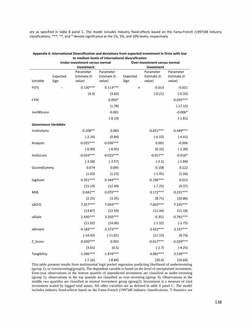
138
are as specified in table 8 panel C. The model includes industry fixed-effects based on the Fama-French (1997)48 industry classifications. ***, **, and * denote significance at the 1%, 5%, and 10% levels, respectively.
Appendix 6: International Diversification and deviations from expected investment in firms with low to medium levels of international diversification
Under-investment versus normal investment
Over-investment versus normal investment
Variable Expected Sign
Parameter Estimate (t-value)
Parameter Estimate (t-value)
Expected Sign
Parameter Estimate (t-value)
Parameter Estimate (t-value)
FSTS - 0.130*** 0.113*** + -0.013 -0.021
(4.3) (3.62) (-0.21) (-0.33)
CYSE 0.003* -0.035***
(1.78) (-17.15)
InvDBScore -0.001 -0.006*
(-0.19) (-1.81)
Governance Variables
Institutions -0.208** 0.083 -0.651*** -0.449***
(-2.24) (0.84) (-6.55) (-4.41)
Analysts -0.025*** -0.036*** 0.001 -0.006
(-6.99) (-8.95) (0.32) (-1.30)
InvGscore -0.024*** -0.025*** -0.017** -0.016*
(-3.58) (-3.57) (-2.1) (-1.84)
GscoreDummy 0.074 0.095 -0.108 0.122
(1.03) (1.23) (-1.45) (1.56)
logAsset 0.351*** 0.344*** -0.196*** 0.012
(15.19) (12.49) (-7.25) (0.37)
MtB 0.042** 0.070*** 0.172*** 0.231***
(2.25) (3.35) (8.71) (10.86)
sdCFO 7.317*** 7.043*** 7.003*** 7.335***
(13.87) (12.59) (11.44) (11.18)
sdSale 2.430*** 3.350*** -0.351 -0.791***
(11.02) (14.06) (-1.32) (-2.75)
sdInvest -4.183*** -3.573*** 3.422*** 3.137***
(-14.43) (-11.81) (11.15) (9.73)
Z_Score 0.020*** 0.003 -0.017*** -0.029***
(3.65) (0.5) (-2.7) (-4.25)
Tangibility -1.396*** -1.874*** 4.082*** 3.539***
(-7.16) (-8.84) (20.4) (16.64)
This table presents results from multinomial logit pooled regression predicting likelihood of underinvesting
(group 1), or overinvesting(group3). The dependent variable is based on the level of unexplained investment.
Firm-year observations in the bottom quartile of unpredicted investment are classified as under-investing
(group 1), observations in the top quartile are classified as over-investing (group 3). Observations in the
middle two quartiles are classified as normal investment group (group2). Investment is a measure of total
investment scaled by lagged total assets. All other variables are as defined in table 8 panel C. The model
includes industry fixed-effects based on the Fama-French (1997)48 industry classifications. T-Statistics are
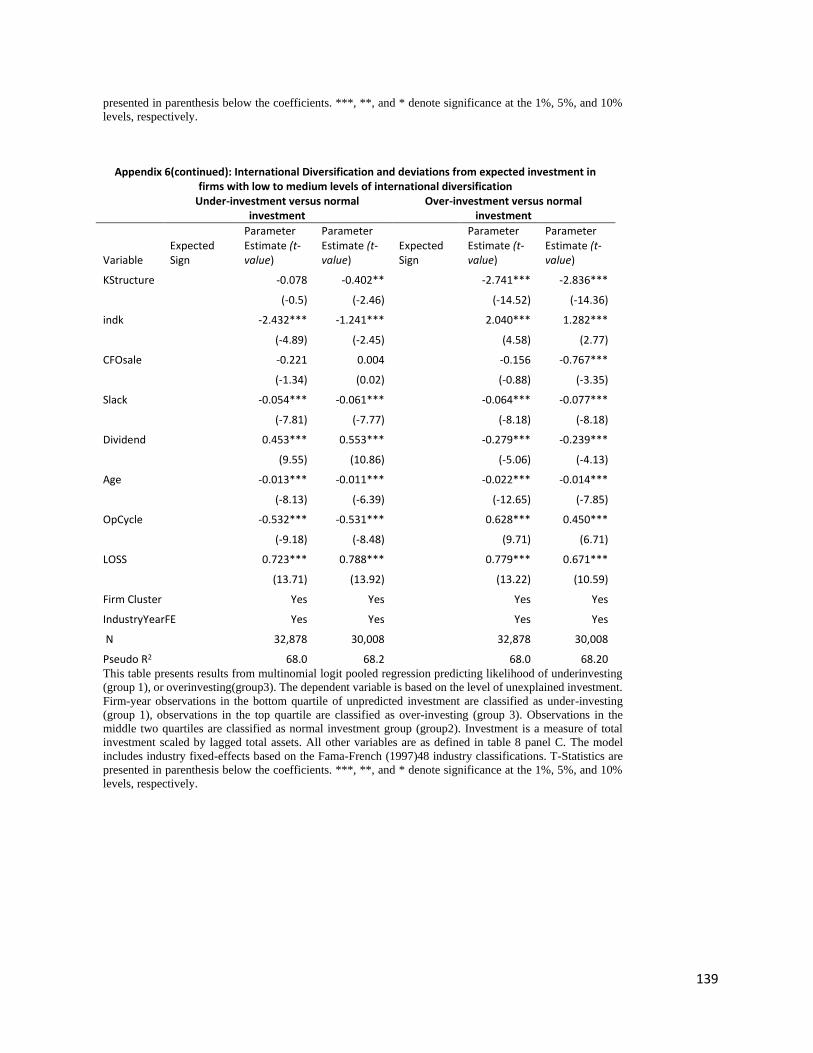
139
presented in parenthesis below the coefficients. ***, **, and * denote significance at the 1%, 5%, and 10%
levels, respectively.
Appendix 6(continued): International Diversification and deviations from expected investment in firms with low to medium levels of international diversification
Under-investment versus normal investment
Over-investment versus normal investment
Variable Expected Sign
Parameter Estimate (t-value)
Parameter Estimate (t-value)
Expected Sign
Parameter Estimate (t-value)
Parameter Estimate (t-value)
KStructure -0.078 -0.402** -2.741*** -2.836***
(-0.5) (-2.46) (-14.52) (-14.36)
indk -2.432*** -1.241*** 2.040*** 1.282***
(-4.89) (-2.45) (4.58) (2.77)
CFOsale -0.221 0.004 -0.156 -0.767***
(-1.34) (0.02) (-0.88) (-3.35)
Slack -0.054*** -0.061*** -0.064*** -0.077***
(-7.81) (-7.77) (-8.18) (-8.18)
Dividend 0.453*** 0.553*** -0.279*** -0.239***
(9.55) (10.86) (-5.06) (-4.13)
Age -0.013*** -0.011*** -0.022*** -0.014***
(-8.13) (-6.39) (-12.65) (-7.85)
OpCycle -0.532*** -0.531*** 0.628*** 0.450***
(-9.18) (-8.48) (9.71) (6.71)
LOSS 0.723*** 0.788*** 0.779*** 0.671***
(13.71) (13.92) (13.22) (10.59)
Firm Cluster Yes Yes Yes Yes
IndustryYearFE Yes Yes Yes Yes
N 32,878 30,008 32,878 30,008
Pseudo R2 68.0 68.2 68.0 68.20
This table presents results from multinomial logit pooled regression predicting likelihood of underinvesting
(group 1), or overinvesting(group3). The dependent variable is based on the level of unexplained investment.
Firm-year observations in the bottom quartile of unpredicted investment are classified as under-investing
(group 1), observations in the top quartile are classified as over-investing (group 3). Observations in the
middle two quartiles are classified as normal investment group (group2). Investment is a measure of total
investment scaled by lagged total assets. All other variables are as defined in table 8 panel C. The model
includes industry fixed-effects based on the Fama-French (1997)48 industry classifications. T-Statistics are
presented in parenthesis below the coefficients. ***, **, and * denote significance at the 1%, 5%, and 10%
levels, respectively.
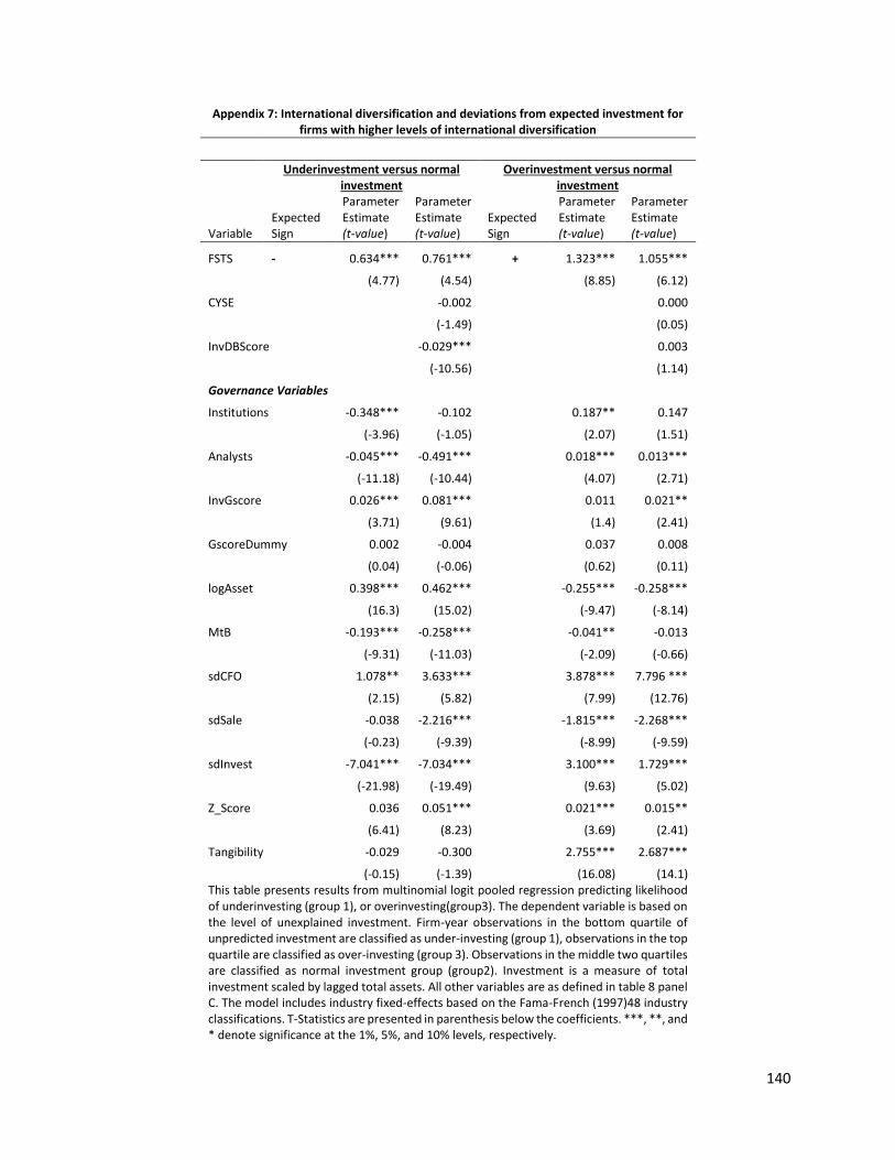
140
Appendix 7: International diversification and deviations from expected investment for firms with higher levels of international diversification
Underinvestment versus normal investment
Overinvestment versus normal investment
Variable Expected Sign
Parameter Estimate (t-value)
Parameter Estimate (t-value)
Expected Sign
Parameter Estimate (t-value)
Parameter Estimate (t-value)
FSTS - 0.634*** 0.761*** + 1.323*** 1.055***
(4.77) (4.54) (8.85) (6.12)
CYSE -0.002 0.000
(-1.49) (0.05)
InvDBScore -0.029*** 0.003
(-10.56) (1.14)
Governance Variables
Institutions -0.348*** -0.102 0.187** 0.147
(-3.96) (-1.05) (2.07) (1.51)
Analysts -0.045*** -0.491*** 0.018*** 0.013***
(-11.18) (-10.44) (4.07) (2.71)
InvGscore 0.026*** 0.081*** 0.011 0.021**
(3.71) (9.61) (1.4) (2.41)
GscoreDummy 0.002 -0.004 0.037 0.008
(0.04) (-0.06) (0.62) (0.11)
logAsset 0.398*** 0.462*** -0.255*** -0.258***
(16.3) (15.02) (-9.47) (-8.14)
MtB -0.193*** -0.258*** -0.041** -0.013
(-9.31) (-11.03) (-2.09) (-0.66)
sdCFO 1.078** 3.633*** 3.878*** 7.796 ***
(2.15) (5.82) (7.99) (12.76)
sdSale -0.038 -2.216*** -1.815*** -2.268***
(-0.23) (-9.39) (-8.99) (-9.59)
sdInvest -7.041*** -7.034*** 3.100*** 1.729***
(-21.98) (-19.49) (9.63) (5.02)
Z_Score 0.036 0.051*** 0.021*** 0.015**
(6.41) (8.23) (3.69) (2.41)
Tangibility -0.029 -0.300 2.755*** 2.687***
(-0.15) (-1.39) (16.08) (14.1) This table presents results from multinomial logit pooled regression predicting likelihood of underinvesting (group 1), or overinvesting(group3). The dependent variable is based on the level of unexplained investment. Firm-year observations in the bottom quartile of unpredicted investment are classified as under-investing (group 1), observations in the top quartile are classified as over-investing (group 3). Observations in the middle two quartiles are classified as normal investment group (group2). Investment is a measure of total investment scaled by lagged total assets. All other variables are as defined in table 8 panel C. The model includes industry fixed-effects based on the Fama-French (1997)48 industry classifications. T-Statistics are presented in parenthesis below the coefficients. ***, **, and * denote significance at the 1%, 5%, and 10% levels, respectively.

141
Appendix 7(continued): International diversification and deviations from expected
investment for firms with higher levels of international diversification
Underinvestment versus normal investment
Overinvestment versus normal investment
Variable Expected Sign
Parameter Estimate (t-value)
Parameter Estimate (t-value)
Expected Sign
Parameter Estimate (t-value)
Parameter Estimate (t-value)
KStructure 0.029 -0.483*** -0.060 -0.085
(0.21) (-3.01) (-0.44) (-0.56)
indk -2.335*** -3.093*** -0.817** -0.779**
(-7.31) (-8.36) (-2.51) (-2.22)
CFOsale -0.036 -0.018 0.141*** 0.149***
(-0.88) (-0.43) (3.42) (3.55)
Slack 0.036*** 0.047*** -0.038*** -0.047***
(8.4) (8.08) (-5.05) (-5.32)
Dividend -0.401*** -0.155** -0.059 0.225***
(-7.85) (-2.56) (-1.17) (3.90)
Age 0.010*** 0.005*** -0.013*** -0.022***
(7.3) (2.86) (-8.8) (-13.03)
OpCycle -0.138*** -0.225*** 0.418*** 0.548***
(-2.8) (-4) (7.94) (9.61)
LOSS 0.433*** 0.658*** 0.200*** -0.014
(7.88) (10.39) (3.5) (-0.22)
Firm Cluster Yes Yes Yes Yes
IndustryYearFE Yes Yes Yes Yes
N 33,785 26,985 33,785 26985
Pseudo R2 (%) 59.10 64.91 59.10 64.91 This table presents results from multinomial logit pooled regression predicting likelihood of underinvesting (group 1), or overinvesting(group3). The dependent variable is based on the level of unexplained investment. Firm-year observations in the bottom quartile of unpredicted investment are classified as under-investing (group 1), observations in the top quartile are classified as over-investing (group 3). Observations in the middle two quartiles are classified as normal investment group (group2). Investment is a measure of total investment scaled by lagged total assets. All other variables are as defined in table 8 panel C. The model includes industry fixed-effects based on the Fama-French (1997)48 industry classifications. T-Statistics are presented in parenthesis below the coefficients. ***, **, and * denote significance at the 1%, 5%, and 10% levels, respectively.
..
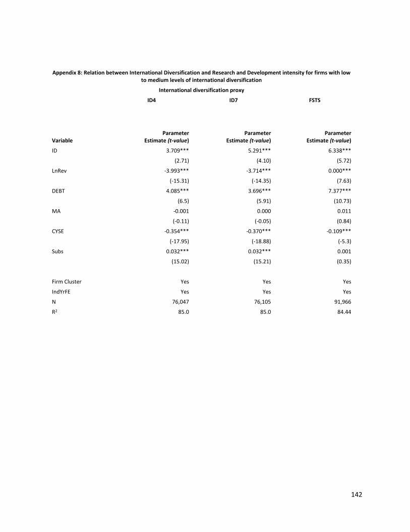
142
Appendix 8: Relation between International Diversification and Research and Development intensity for firms with low to medium levels of international diversification
International diversification proxy
ID4 ID7 FSTS
Variable Parameter
Estimate (t-value) Parameter
Estimate (t-value) Parameter
Estimate (t-value)
ID 3.709*** 5.291*** 6.338***
(2.71) (4.10) (5.72)
LnRev -3.993*** -3.714*** 0.000***
(-15.31) (-14.35) (7.63)
DEBT 4.085*** 3.696*** 7.377***
(6.5) (5.91) (10.73)
MA -0.001 0.000 0.011
(-0.11) (-0.05) (0.84)
CYSE -0.354*** -0.370*** -0.109***
(-17.95) (-18.88) (-5.3)
Subs 0.032*** 0.032*** 0.001
(15.02) (15.21) (0.35)
Firm Cluster Yes Yes Yes
IndYrFE Yes Yes Yes
N 76,047 76,105 91,966
R2 85.0 85.0 84.44

143
Appendix 9: Relation between International Diversification and Research and Development intensity for firms with higher levels of international diversification
International diversification proxy
ID4 ID7 FSTS
Variable Parameter
Estimate (t-value) Parameter
Estimate (t-value) Parameter
Estimate (t-value)
ID -40.540*** -40.494*** 0.845***
(-4.79) (-4.86) (4.16)
LnRev -1.575*** -1.678*** 0.000***
(-3.82) (-4.05) (3.38)
DEBT 13.337*** 13.907*** 6.150***
(12.56) (13.09) (8.14)
MA 0.025 0.026 0.008
(0.87) (0.89) (0.74)
CYSE -0.256*** -0.255*** -0.207***
(-7.55) (-7.36) (-8.96)
Subs 0.016*** 0.015*** 0.004
(3.97) (3.83) (1.53)
Firm Cluster Yes Yes Yes
IndYrFE Yes Yes Yes
N 76,033 75,993 92,117
R2 79.3 79.3 78.3

144
Appendix 10: Effect of international diversification on the relation between R&D investments and variability of future benefits
ID MEASURE = FSTS Model: SD (St+1, t+5) = α+ β1RND t + β2ID + β3RNDt *ID + β4ADEX t + β5FLEV t + β6MV t + Errort+1, t+5
International Diversification Proxy = FSTS
Operating Income CashFlow Sales
FSTS 0.000*** 0.000*** 0.026***
(12.35) (7.37) (4.22)
RND 0.101*** 0.294*** 0.485***
(13.1) (12.78) (5.4)
RND*FSTS -0.001*** -0.001*** -0.615***
(-7.6) (-5.7) (-4.28)
CAPEX 0.051*** 0.399*** 0.400***
(4.96) (12.54) (9.76)
ADEX -0.056*** 0.286*** -0.018
(-2.67) (3.7) (-0.76)
FLEV 0.085*** 0.383*** 0.000
(27.04) (40.57) (0.02)
mv -0.005*** -0.016*** 0.000
(-32.29) (-37.18) (-1.54)
Firm & Year Cluster Yes Yes Yes
N 81,351 81,342 64,249
Adjusted R2(%) 20.37 30.95 20.21 The table presents OLS regressions clustered by firm and year. All variables except MV and FLEV are deflated by stock price at the end of fiscal year t-1. RND is the research and development expense per share, CAPEX is the capital expenditures per share. ADEX is the advertising expense per share. MV is the natural logarithm of the market value at the end of year t. FLEV is the book value of debt divided by the sum of debt and market value of equity at the end of fiscal year t. Earnings is the earnings per share before extraordinary items and discontinued operations. Sd (Sale t+1, t+5) is the standard deviation of sales revenue. Standard deviations are calculated using five annual observations for years t+1 to t+. Data is winsorized at the top and bottom 1 percent of observations.
145
References
Allison, P. D. (2006). Fixed effects regression methods in SAS. SUGI 31 Proceedings, 1, 20. Agrawal, A., Jaffe, J. F., & Mandelker, G. N. (1992). The post‐merger performance of
acquiring firms: a re‐examination of an anomaly. The Journal of Finance, 47(4), 1605-1621. Allen, L., & Pantzalis, C. (1996). Valuation of the operating flexibility of multinational
corporations. Journal of international business studies, 27(4), 633-653. Andrade, G., Mitchell, M., & Stafford, E. (2001). New evidence and perspectives on
mergers. The Journal of Economic Perspectives, 15(2), 103. Amberger, H. J., Markle, K. S., & Samuel, D. M. (2021). Repatriation taxes, internal agency
conflicts, and subsidiary-level investment efficiency. The Accounting Review, 96(4), 1-25. Amihud, Y., De Long, G., & Saunders, A. (2002). The effects of cross-border bank mergers
on bank risk and value. Journal of International Money and Finance, 21, 857–877 Amihud, Y., & Lev, B. (1981). Risk reduction as a managerial motive for conglomerate
mergers. The bell journal of economics, 605-617. Amir, E., Guan, Y., & Livne, G. (2007). The Association of R&D and Capital Expenditures
with Subsequent Earnings Variability. Journal of Business Finance & Accounting, 34(1/2), 222-246.
Asdemir, O., Anderson, M., & Tripathy, A. (2012). Use of precedent and antecedent information in strategic cost management.
Autor, D., William R. Kerr, & Kugler, A. (2007). Does Employment Protection Reduce Productivity? Evidence from US States. The Economic Journal, 117(521), F189-F217. Retrieved from http://www.jstor.org/stable/4625523
Banker, R. D., Byzalov, D., & Plehn-Dujowich, J. M. (2014). Demand uncertainty and cost behavior. Accounting review: A quarterly journal of the American Accounting Association, 89(3), 839-865.
Banker, R. D., Mashruwala, R., & Tripathy, A. (2014b). Does a differentiation strategy lead to more sustainable financial performance than a cost leadership strategy? Management Decision, 56(5), 872-896.
Biddle, G. C., Hilary, G., & Verdi, R. S. (2009). How does financial reporting quality relate to investment efficiency? Journal of Accounting and Economics, 48(2), 112-131.
Buckley, P. J. (1988). The limits of explanation: Testing the internalization theory of the multinational enterprise. Journal of international business studies, 181-193.
Capar, N., & Kotabe, M. (2003). The relationship between international diversification and performance in service firms. Journal of international business studies, 34(4), 345-355.
Caves, R. E. (1989). Mergers, takeovers, and economic efficiency: foresight vs. hindsight. International Journal of Industrial Organization, 7(1), 151-174.
Caves, R. E. (1996). Multinational enterprise and economic analysis. Cambridge university press.
Chay, J. B., & Suh, J. (2009). Payout policy and cash-flow uncertainty. Journal of Financial Economics, 93(1), 88-107.
Child, J., Faulkner, D., & Pitkethly, R. (2001). The management of international acquisitions. OUP Oxford.
146
Cette, G., Lopez, J., & Mairesse, J. (2016). Labour Market Regulations and Capital Intensity (No. w22603). National Bureau of Economic Research.
Davidson, W. (1983). Market similarity and market selection: Implications for international marketing strategy. Journal of Business Research, 11(4), 439-456. doi:10.1016/0148-2963(83)90004-8
Delios, A., & Beamish, P. W. (1999). Geographic scope, product diversification, and the corporate performance of Japanese firms. Strategic Management Journal, 711-727.
Delios, A., & Henisz, W. I. (2000). Japanese firms' investment strategies in emerging economies. Academy of Management journal, 43(3), 305-323.
Denis, D. J., Denis, D. K., & Yost, K. (2002). Global diversification, industrial diversification, and firm value. The Journal of Finance, 57(5), 1951-1979.
Dess, G. G., Ireland, R. D., & Hitt, M. A. (1990). Industry effects and strategic management research. Journal of management, 16(1), 7-27.
Engel, C., & Matsumoto, A. (2009). The international diversification puzzle when goods prices are sticky: it's really about exchange-rate hedging, not equity portfolios. American economic Journal: macroeconomics, 1(2), 155-88.
Gomes, L., & Ramaswamy, K. (1999). An Empirical Examination of The Form of The Relationship Between Multinationality and Performance. Journal of International Business Studies, 173-187.
Hasan, R., Mitra, D., & Sundaram, A. (2013). The determinants of capital intensity in manufacturing: the role of factor market imperfections. World Development, 51, 91-103.
Hill, C. W., & Snell, S. A. (1988). External control, corporate strategy, and firm performance in research‐intensive industries. Strategic Management Journal, 9(6), 577-590.
Hill, C. W., & Snell, S. A. (1989). Effects of ownership structure and control on corporate productivity. Academy of Management journal, 32(1), 25-46.
Hisey, K. B., & Caves, R. E. (1985). Diversification strategy and choice of country: diversifying acquisitions abroad by US multinationals, 1978–1980. Journal of International Business Studies, 16(2), 51-64.
Hitt, M. A., Hoskisson, R. E., & Kim, H. (1997). International diversification: Effects on innovation and firm performance in product-diversified firms. Academy of Management journal, 40(4), 767-798.
Hitt, M. A., Hoskisson, R. E., & Ireland, R. D. (1994). A mid-range theory of the interactive effects of international and product diversification on innovation and performance. Journal of management, 20(2), 297-326.
Hope, O. K., & Thomas, W. B. (2008). Managerial empire building and firm disclosure. Journal of Accounting Research, 46(3), 591-626.
Hoskisson, R. E. (1987). Multidivisional structure and performance: The contingency of diversification strategy. Academy of Management journal, 30(4), 625-644.
Hoskisson, R. E., & Hitt, M. A. (1990). Antecedents and Performance Outcomes of Diversification: A Review and Critique of Theoretical Perspectives. Journal Of Management, 16(2), 461.
Hsu, C. C., & Boggs, D. J. (2003). Internationalization and performance: Traditional measures and their decomposition. Multinational Business Review, 11(3), 23-50.
147
Jensen, M. C. (1986). Agency costs of free cash flow, corporate finance, and takeovers. The American economic review, 76(2), 323-329.
Jensen, M. C., & Meckling, W. H. (1976). Theory of the firm: Managerial behavior, agency costs and ownership structure. Journal of financial economics, 3(4), 305-360.
Kothari, S. P., Laguerre, T. E., & Leone, A. J. (2002). Capitalization versus Expensing: Evidence on the Uncertainty of Future Earnings from Capital Expenditures versus R&D Outlays. Review Of Accounting Studies, 7(4), 355-382.
Kravis, I. B., & Lipsey, R. E. (1982). The location of overseas production and production for export by US multinational firms. Journal of international economics, 12(3-4), 201-223.
Lane, P. J., Cannella Jr, A. A., & Lubatkin, M. H. (1998). Agency problems as antecedents to unrelated mergers and diversification: Amihud and Lev reconsidered. Strategic Management Journal, 555-578.
Larsson, R., & Finkelstein, S. (1999). Integrating strategic, organizational, and human resource perspectives on mergers and acquisitions: A case survey of synergy realization. Organization science, 10(1), 1-26.
Lipsey, R. E., Kravis, I. B., & Roldan, R. A. (1982). Do multinational firms adapt factor proportions to relative factor prices?. Trade and employment in developing countries: Factor supply and substitution, 215-55.
Lubatkin, M. (1983). Mergers and the Performance of the Acquiring Firm. Academy of Management review, 8(2), 218-225.
Lu, J. W., & Beamish, P. W. (2004). International diversification and firm performance: The S-curve hypothesis. Academy of management journal, 47(4), 598-609.
Meyer, M., Milgrom, P., & Roberts, J. (1992). Organizational prospects, influence costs, and ownership changes. Journal of Economics & Management Strategy, 1(1), 9-35.
McGee, T., Thomson, R., & Thomas, T. (2014). Merger and Acquisitions Trends Report 2014. Deloitte.com. Retrieved April 13, 2015, from http://www2.deloitte.com/us/en/pages/
Porter, M. E., Goold, M., & Luchs, K. (1996). From competitive advantage to corporate strategy. Managing the multibusiness company. Strategic issues for diversified groups, 285, 285-314.
Porter, M. E. The Competitive Advantage: Creating and Sustaining Superior Performance. NY: Free Press, 1985. (Republished with a new introduction, 1998.)
Ramaswamy, K. 1995. Multinationality, configuration,and performance: A study of MNCs in the U.S. drug and pharmaceutical industry. Journal of International Management, 1: 231–253
Ravenscraft, D. J., & Scherer, F. M. (1987). Life after takeover. The Journal of Industrial Economics, 147-156.
Ravenscraft, D. J., & Scherer, F. M. (1989). The profitability of mergers. International journal of industrial organization, 7(1), 101-116.
Richardson, S. (2006). Over-investment of free cash flow. Review of accounting studies, 11(2-3), 159-189.
Rindova, V. P., & Fombrun, C. J. (1999). Constructing competitive advantage: The role of firm-constituent interactions. Strategic management journal, 691-710.
Ruigrok, W., & Wagner, H. (2003). Internationalization and performance: An organizational learning perspective. MIR: Management International Review, 63-83.
Rumelt, R. P. (1982). Diversification Strategy and Profitability. Strategic Management Journal, 3(4), 359-369.
148
Shimizu, K., Hitt, M. A., Vaidyanath, D., & Pisano, V. (2004). Theoretical foundations of cross-border mergers and acquisitions: A review of current research and recommendations for the future. Journal of international management, 10(3), 307-353.
Stobaugh, R. B. Jr., Where in the World Should We Put that Plant, Harvard Bus.Rev. (January-February 1969): 31-37.
Thomas, D. E., & Eden, L. (2004). What is the shape of the multinationality-performance relationship? Multinational Business Review, 12(1), 89-110.
Tosi Jr, H. L., & Gomez-Mejia, L. R. (1989). The decoupling of CEO pay and performance: An agency theory perspective. Administrative Science Quarterly, 169-189.
Vander Vennet, R., & Gropp, R. (2003). Cross-border mergers in European banking and bank efficiency. In Foreign direct investment in the real and financial sector of industrial countries (pp. 295-321). Springer Berlin Heidelberg.
Weber, Y., Tarba, S. Y., & Oberg, C. (2013). A Comprehensive Guide to Mergers & Acquisitions: Managing the Critical Success Factors Across Every Stage of the M&A Process. Pearson Education.
Wheeler, David (08/1992). "International investment location decisions". Journal of international economics (0022-1996), 33 (1-2), p. 57.
DOI: 10.1016/0022-1996(92)90050-T Zaheer, S., 1995. Overcoming the liability of foreignness. Acad. Manage. J. 38, 341–363. Zahra, S. A., Ireland, R. D., & Hitt, M. A. (2000). International expansion by new venture
firms: International diversity, mode of market entry, technological learning, and performance. Academy of Management journal, 43(5), 925-950.