1

The 7th International Supercritical CO2 Power Cycles Symposium March 31 – April 2, 2020, San Antonio, Texas

Paper #113, NETL-PUB-22738

COOLING SYSTEM COST AND PERFORMANCE MODELS TO MINIMIZE COST OF ELECTRICITY OF DIRECT SCO2 POWER PLANTS

Sandeep R. Pidaparti KeyLogic

Pittsburgh, PA, U.S.A.

Charles W. White KeyLogic

Fairfax, VA, U.S.A.

Nathan T. Weiland* National Energy Technology Laboratory

Pittsburgh, PA, U.S.A. nathan.weiland@netl.doe.gov

ABSTRACT

The performance of direct-fired (direct) sCO2 power cycles can be improved by reducing the sCO2 cooler temperature in order to increase the sCO2 density at the inlet to the compressor and pump, thereby reducing the specific power required for compression and increasing the net power and thermal efficiency of the sCO2 cycle. For a given ambient temperature, the achievable sCO2 cooler temperature depends on the size and operating conditions of the cooling technology, which in turn affects the cooling system capital cost. Hence a plant’s cost of electricity (COE) can be minimized with respect to its cooling system by balancing fuel cost (efficiency) against plant’s capital cost distributed over the lifetime of the plant.

The present study reviews spreadsheet performance and cost models of four different cooling technologies that were originally developed for indirect (externally heated) sCO2 plants: wet cooling towers, indirect dry coolers, direct dry coolers, and adiabatic coolers. These models are extended to include the direct sCO2 cycle working fluids that contain impurities and are then applied to a natural gas-fueled direct sCO2 power plant. For a given set of design ambient conditions, the plant’s COE is minimized for each of the cooler types as a function of sCO2 cooler temperature and cooler operating conditions. Results indicate that, depending on the cooling technology, the plant efficiency is shown to improve by 1.7 – 2.4 percentage points and the plant COE is reduced by up to 4.2%, by lowering sCO2 cooler outlet temperature from 35 to 20 °C. Further, the direct cooling approaches are shown to offer the potential for the lowest plant COE for the given plant design and ambient conditions in this study.

INTRODUCTION

The direct-fired supercritical CO2 (sCO2) power cycle, often referred to as the Allam cycle in the literature, is being pursued as an attractive alternative to the NGCC and IGCC plants with carbon capture and storage (CCS) [1, 2]. The cycle employs oxy-combustion of either natural gas [1] or coal-derived syngas [2] in a dilute sCO2 environment to generate combustion products that drive the turbine. The remaining thermal energy from the turbine exhaust is recuperated to heat the sCO2 diluent flow to the combustor. After recuperation, water is condensed out of the product stream and a portion of the working fluid (primarily CO2) is drawn from the cycle for further purification and storage. Rest of the working fluid (sCO2 diluent) is compressed to the cycle maximum pressure for preheating in the recuperator and return to the combustor.

2

One of the inherent advantages of the direct-fired sCO2 power cycle is that it generates a CO2 product stream at high pressures typical of CO2 storage systems. The high operating pressure (typically ~300 bar) and low cycle pressure ratio (typically ~10) allow for use of compact turbomachinery and heat exchangers. The sCO2 diluent compression train, which includes the pre-compressor and the pump, take advantage of the high working fluid density near the critical point to reduce the specific power required for compression and hence increase the power output of the cycle. NETL conducted a preliminary techno-economic analysis of natural gas-fueled version of the direct-fired sCO2 power cycle for cold end sCO2 temperature of 26.7 °C [3]. The preliminary results showed that the sCO2 plant efficiency is 2.5 percentage points higher and cost of electricity (COE) is 4.9% lower than a reference NGCC plant with CCS [3, 4].

Reducing the cold end sCO2 temperature (referred to as sCO2 cooler temperature in rest of the paper) increases the sCO2 diluent density and reduces the compression power, thereby increasing the cycle efficiency further. On the contrary, the cooling system capital costs and auxiliary power consumption increase as the sCO2 cooler temperature approaches the ambient design temperature (wet or dry bulb temperatures). Therefore, it is important to investigate the tradeoffs between increase in cycle efficiency (through reduction of sCO2 cooler temperature) and increase in the cooling system capital costs in order to minimize a plant’s COE.

Recently, NETL conducted a similar analysis for coal-fueled indirect-fired sCO2 power cycles [5], in which performance and cost spreadsheet models were developed for four different cooling technologies (wet cooling tower [6], indirect dry cooling [7], direct dry cooling [8] and adiabatic cooling [9]) and the impact of these cooling technologies on plant efficiency and COE was evaluated. The study showed that the plant efficiency can be increased by 3-4 percentage points, and COE can be reduced by up to 8%, through appropriate selection of sCO2 cooler temperature, cooling technology, and cooling system operating conditions. These models are publicly available to aid cycle designers in optimizing their plant’s cooling system and COE [10].

In light of above discussion, the objective of the current study is to conduct techno-economic analyses (TEA) to optimize the COE of natural gas-fueled direct-fired sCO2 power plants as a function of the sCO2 cooler temperature, cooling technology, and the cooling system operating conditions. The paper will first provide details about the direct sCO2 power plant configuration, plant modeling and economic analysis methodology. The paper will then describe the approach taken to calculate the sCO2 mixture properties within the cooling technology models. For each of the cooling technologies, the optimization variables and optimization procedure will be described, followed by discussion of results.

DIRECT SCO2 POWER PLANT CONFIGURATION

Figure 1 presents a block flow diagram for the natural gas-fueled direct sCO2 power plant of interest in the present study and the associated state points for a sCO2 cooler temperature of 26.7 °C. The prior NETL study included a low pressure air separation unit (ASU) followed by oxygen compression to 64.1 bar prior to mixing with sCO2 diluent stream [3]. Due to potential concerns associated with compression and handling of pure oxygen, the revised plant shown in Figure 1 includes a high pressure cryogenic ASU with an oxygen discharge pressure of 100 bar (stream 2 in Figure 1). This oxygen is premixed with portion of the sCO2 recycle stream to achieve an oxidant stream with a maximum oxygen mole fraction of 23.5%, which is then pressurized to the cycle maximum pressure of ~308 bar in the oxidant compressor (OC).

The recuperation train is split into three stages to better manage the thermal pinch points and maximize the heat recovery from ASU. The recuperation train, which includes a low temperature

3

recuperator (LTR), an intermediate temperature recuperator (ITR) and a high temperature recuperator (HTR), uses the low-pressure hot turbine exhaust to preheat the high pressure sCO2 diluent and the oxidant streams before they enter the combustor. The LTR is designed to handle the condensation of water vapor from turbine exhaust stream, thus the hot end inlet temperature to the LTR (stream 27 in Figure 1) is typically at or close to the dew point. Following the LTR, additional cooling is employed to knockout most of the remaining water vapor prior to compression up to 100 bars in an intercooled pre-compressor (PC), followed by additional cooling and pumping (P, OC) to the maximum cycle pressure. A portion of the high pressure sCO2 diluent stream is split off after exiting the LTR (stream 16 in Figure 1) and is heated in parallel with the ITR using process heat from ASU’s main air compressor (MAC) and boost air compressor (BAC) intercoolers. A portion of this split stream is used as the source for the turbine blade cooling flow (stream 18 in Figure 1) and the rest (stream 19 in Figure 1) is mixed with high pressure sCO2 diluent flow exiting ITR. The oxidant and sCO2 diluent streams undergo final preheating in the HTR before they enter the combustor. The cycle’s purge stream (stream 30 in Figure 1) is purified in a cryogenic CO2 processing unit (CPU, not shown) to meet CO2 pipeline standards for oxygen, CO, water and other contaminants [11].

Figure 1: Block flow diagram for the revised natural gas-fueled direct fired sCO2 power plant

ANALYSIS METHODOLOGY

A steady-state model of the plant in Figure 1 was developed using Aspen Plus® (Aspen). The plant modeling approach and the assumptions used are described below followed by a brief description of the economic analysis methodology.

sCO2 Plant Modeling and Assumptions

Accurate modeling of direct-fired sCO2 power plants requires accurate calculation of sCO2 mixture thermophysical properties, particularly near the critical point. Due to the difficulties associated with the Span-Wagner equation of state (EOS) for sCO2 mixtures, the Lee-Kesler Plöcker (LKP) EOS was used for modeling of the sCO2 plant in Aspen. The decision to use LKP EOS was based on a prior study which identified this EOS to be the most accurate for use in direct fired sCO2 power cycle modeling [12].

Purgeto CPU

P

TPC

100 bar O215 °C

H2O

Combustor

Turbine

ASUAir

LTR HTR

Cooling sCO2

sCO2+O2

MAC/BAC

sCO2

Nat. Gas

ITR

OCsCO2+O2

5

11

12

14

6

2

819

1

3

7

9

20

17

15

1618

4

10

21

22

2324

25262729

30

88.9 MW/43.9 MW

69.5 MWt

3°C 63.5 MWt34 °C

20.0 MW27 °C

27° C 27 °C

27 °C

116 °C 251 °C 757 °C

219 °C

219 °C

219 °C

219 °C

105 °C

105 °C

106 °C 722 °C

722 °C

1204 °C40 °C

35.0 MW

100.8 MW 925.7 MW

712.5 MWth

318.3 MWth

1030.8 MWth

164.1 MWth

84.4 MWth

248.5 MWth

23.7 %

27.9 %

26.5 %

47° C

N2Med & low qual heat to ASU & CW

High qual heat to power cycle

55 °C

40 °C 153.6 MWt

67.7 MWt

221.3 MWt28

MC

KO Cooler

4

The oxy-combustor is modeled in Aspen as a series of combustion reactions for the oxidizable components of the fuel and assuming 100 percent conversion of these fuel components. The amount of excess oxygen was calculated based on the stoichiometric amount needed for complete combustion of the fuel entering the combustor, without regard to any oxidizable components in recycle sCO2 stream. The pressure drop through the combustor is assumed to be 689 kPa and the heat loss is assumed be zero. The combustor outlet temperature of 1204 °C is met by adjusting the sCO2 recycle flow rate.

The turbine inlet temperature of 1204 °C is high enough to require turbine blade cooling. An empirical turbine cooling model, based on modeling data from an IEAGHG study [13], was used to calculate the turbine coolant flow as a function of the coolant temperature. The model is based on a correlation between gross cooling effectiveness and heat loading parameter [3, 4].

The sCO2 cycle recuperators (LTR, ITR and HTR) are modeled as adiabatic counterflow heat exchangers with perfect thermal mixing in the transverse direction and negligible heat transfer in the axial direction. A minimum temperature approach of 10 °C is enforced within the recuperation train. The minimum temperature approach typically occurred at the hot ends of HTR and LTR due to heat integration with the ASU. The total pressure drop across the recuperation train is set to 137.9 kPa (20 psi) for both the hot and cold sides.

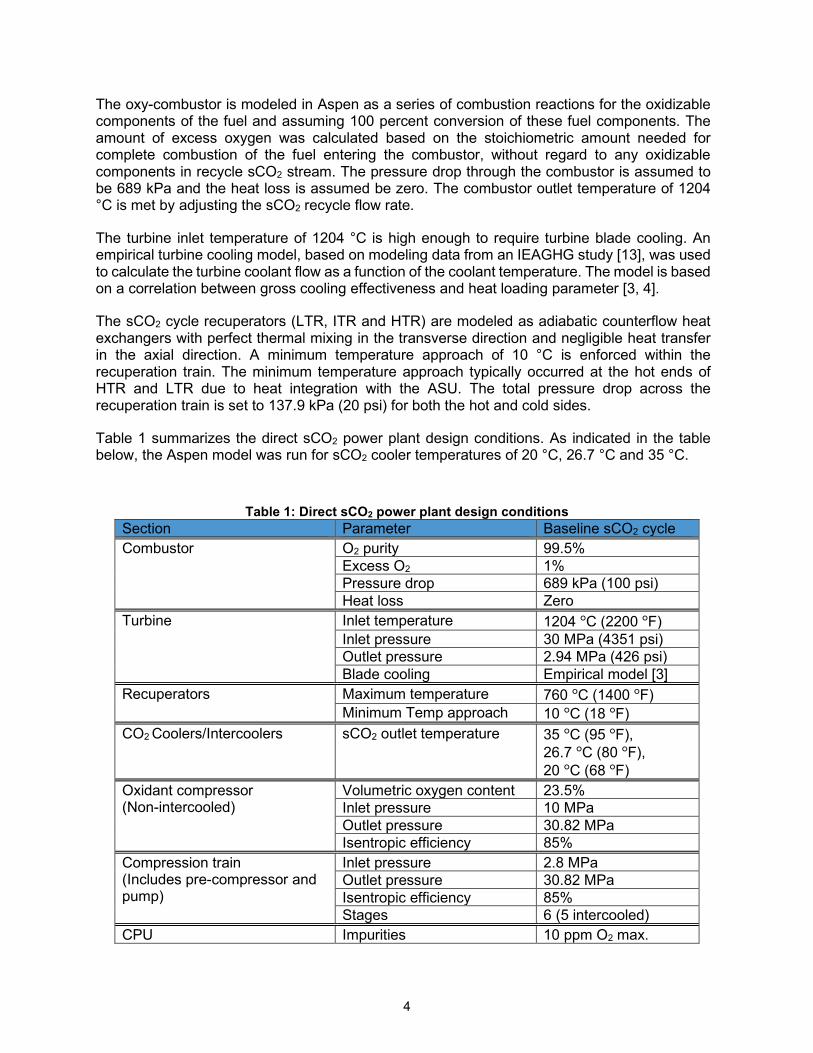
Table 1 summarizes the direct sCO2 power plant design conditions. As indicated in the table below, the Aspen model was run for sCO2 cooler temperatures of 20 °C, 26.7 °C and 35 °C.

Table 1: Direct sCO2 power plant design conditions

Section Parameter Baseline sCO2 cycle Combustor O2 purity 99.5%

Excess O2 1% Pressure drop 689 kPa (100 psi) Heat loss Zero

Turbine Inlet temperature 1204 °C (2200 °F) Inlet pressure 30 MPa (4351 psi) Outlet pressure 2.94 MPa (426 psi) Blade cooling Empirical model [3]

Recuperators Maximum temperature 760 °C (1400 °F) Minimum Temp approach 10 °C (18 °F)

CO2 Coolers/Intercoolers sCO2 outlet temperature 35 °C (95 °F), 26.7 °C (80 °F), 20 °C (68 °F)

Oxidant compressor (Non-intercooled)

Volumetric oxygen content 23.5% Inlet pressure 10 MPa Outlet pressure 30.82 MPa Isentropic efficiency 85%

Compression train (Includes pre-compressor and pump)

Inlet pressure 2.8 MPa Outlet pressure 30.82 MPa Isentropic efficiency 85% Stages 6 (5 intercooled)

CPU Impurities 10 ppm O2 max.

5

The compression train includes pre-compressor (PC) and pump (P). The pre-compressor is modeled as a four-stage compressor with three intercoolers followed by an aftercooler (labelled as “MC” in Figure 1). The three intercoolers for pre-compressor will be referred to as “PCIC1”, “PCIC2” and “PCIC3” in the rest of the paper. The pump (P) is a modeled as a two-stage compressor with single stage of intercooling. The pump intercooler will be referred to as “PIC” in the rest of the paper. The compression train pressure profiles are adjusted for each sCO2 cooler temperature to maximize the cycle efficiency and provide split stream for mixing with the oxygen from ASU. The compression train pressure profiles for sCO2 cooler temperatures of 20 °C, 26.7 °C and 35 °C are presented on a pressure-enthalpy (P-h) diagram in Figure 2. Note that the saturated vapor and liquid lines on the figure are for the direct sCO2 recycle fluid mixture, which results in higher saturation pressures than those for pure CO2.

Figure 2: Compression train details for sCO2 cooler temperatures of 20, 26.7 and 35 °C

For sCO2 cooler temperatures greater than the critical temperature of sCO2 mixture (35 °C in Figure 2), the PC exit pressure is set to 100 bar to match the oxygen pressure leaving ASU and the pressure ratio for all the stages of the PC are equal. For sCO2 cooler temperatures lower than the critical temperature (20 °C, 26.7 °C in Figure 2), exit pressure for the third stage of the PC is set to bubble point pressure for that particular sCO2 cooler temperature and the pressure ratio is equal for the first three stages. The exit pressure for the fourth stage of the PC is set to 100 bar to match the oxygen pressure leaving ASU. After a portion of the sCO2 diluent is mixed with oxygen from the ASU, rest of the sCO2 diluent is pressurized to ~308 bar in an intercooled pump (P) with equal pressure ratio stages. Table 2 summarizes the design conditions for all the sCO2 process coolers (PCIC1, PCIC2, PCIC3, MC, PIC) for sCO2 cooler temperatures of 20 °C, 26.7 °C and 35 °C.

2

6

10

14

18

22

26

30

34

200 250 300 350 400 450 500 550

Pres

sure

(MPa

)

Enthalpy (kJ/kg)

sCO2 cooler temperature - 20CsCO2 cooler temperature - 26.7CsCO2 cooler temperature - 35C

6

Table 2: sCO2 process coolers operating conditions for different sCO2 cooler temperatures; 𝑻𝑻𝒊𝒊𝒊𝒊 and 𝑷𝑷𝒊𝒊𝒊𝒊 are the temperature and pressure of sCO2 stream entering the cooler, 𝑻𝑻𝒐𝒐𝒐𝒐𝒐𝒐 is the

temperature of sCO2 stream leaving the cooler, �̇�𝒎 is the mass flow rate of sCO2 stream sCO2 cooler temperature Cooler Heat Duty

(MWth) 𝑇𝑇𝑖𝑖𝑖𝑖 (°C)

𝑃𝑃𝑖𝑖𝑖𝑖 (MPa)

𝑇𝑇𝑜𝑜𝑜𝑜𝑜𝑜 (°C)

�̇�𝑚 (kg/s)

20 °C

PCIC1 58.8 49.1 3.987 20.0 1607.4 PCIC2 81.7 49.5 5.669 20.0 1607.4 PCIC3 278.9 48.2 8.059 20.0 1607.4

MC 18.8 23.7 10.080 20.0 1607.4 PIC 25.6 31.8 17.613 20.0 1181.6

26.7 °C

PCIC1 61.9 58.1 4.078 26.7 1607.3 PCIC2 83.3 58.6 5.928 26.7 1607.3 PCIC3 247.7 57.5 8.618 26.7 1607.3

MC 31.2 30.9 10.080 26.7 1607.3 PIC 36.0 39.5 17.613 26.7 1181.9

35 °C

PCIC1 52.3 62.6 3.878 35.0 1607.2 PCIC2 61.7 62.5 5.342 35.0 1607.2 PCIC3 85.1 62.3 7.362 35.0 1607.2

MC 178.2 60.6 10.080 35.0 1607.2 PIC 96.4 57.0 17.613 35.0 1181.7

Economic Analysis Methodology

Based on the steady-state modeling results, operating conditions of the cycle and balance of plant components are used to estimate costs for equipment, installation, contractor fees, and contingencies. Following a standard cost estimating methodology [14, 15], these are summed to arrive at a total plant cost (TPC), expressed in June 2011 dollars for consistency with other NETL studies [16, 17]. Using a consistent methodology and set of assumptions [15], owner’s costs are also calculated and added to the TPC to arrive at the total overnight cost (TOC), which is used in the COE calculation.

sCO2 Cycle Component Cost Estimates

No cost estimates are available in public domain for the combustor and turbine. The approach taken with this component is to combine the cost of a similarly-sized gas turbine (without the compressor) with the cost of high-pressure outer casing similar to those used for HP stream turbines. Costs for these components are well-known and combine to constitute a cost estimate for a mature, nth-of-a-kind (NOAK) direct sCO2 turbine and combustor, albeit with a high degree of uncertainty.

Rest of the sCO2 cycle component capital costs are calculated using component cost algorithms developed under prior work for indirect fired sCO2 power cycle applications [18]. The sCO2 diluent, oxidant compressors and pumps are commercially available, and their costs are estimated using a volumetric flow-based cost scaling algorithm developed from vendor quotes. The recuperator capital costs are calculated using a conductance (𝑈𝑈𝑈𝑈)-based cost scaling algorithm. Recuperator conductance is calculated using discretized heat exchanger model that includes 100 segments (of equal heat duty) in the direction of flow. The recuperator cost scaling algorithm includes a temperature correction factor for maximum temperatures greater than 550 °C [18]. Therefore, to reduce the capital cost, HTR is split into two units when the hot side fluid temperature is at 550 °C and the two units are assumed to be installed in series. Capital cost

7

estimation methodology for the cooling system is unique to type of cooling system and will be described in the subsequent sections.

Other Capital Cost Estimates

Aside from the power cycle, the balance of plant unit operations and equipment items are analogues to an NGCC plant. The cost estimates for these items are based on a combination of vendor data, estimates from Worley-Parsons, power law scaling and correlations that were fit to historical cost estimates published in previous NETL reports [17].

Cost scaling algorithms with reference costs and reference process variable data were taken from the reference NGCC plant analysis, which are consistent with published cost scaling guidelines [14]. The same BOP cost accounts as for the NGCC plant were used except that there is no steam generator or HRSG and some of the sub-accounts from the NGCC plant did not apply, including the feedwater and miscellaneous BOP system and steam turbine building.

Following this methodology, capital cost estimates are expected to have an accuracy in the -15% to +50% range. Since the direct sCO2 power cycles are in the demonstration stage, the accuracy range is consistent with an AACE Class 4 feasibility study designation.

Cost of Electricity (COE) Calculation

The COE consists of five components representing normalized contributions from capital costs, fixed operations & maintenance (O&M) costs, variable O&M costs, fuel costs, and the transportation & storage (T&S) costs for captured CO2. These are calculated following a consistent methodology used in all NETL studies [15]. The financial assumptions used in the COE calculation for the sCO2 plant are detailed elsewhere [4] but are identical to those used for the reference NGCC plant with CCS [17], including the capacity factor (85%), natural gas fuel price ($6.13/MMBtu), plant construction period (3 years), operating lifetime (30 years), staffing (6 operators/shift), and other financing assumptions.

COOLING SYSTEM MODELS

This section summaries the technical basis for performance and cost models for the four cooling technologies explored in this study.

sCO2 Mixture Properties

As noted above, the spreadsheet-based cooling system models were originally developed for indirect sCO2 power plants where the working fluid is pure CO2. However, in the case of direct-fired sCO2 power plants the working fluid is a sCO2 mixture with trace amounts argon, nitrogen, oxygen, water vapor, and other species. The thermophysical properties of this sCO2 mixture are calculated by linking the Excel spreadsheet-based cooling system models to REFPROP v10 [19]. Flash calculations for sCO2 mixtures tend to fail near the critical point when using REFPROP due to the presence of water vapor in the mixture, consistent with the findings of prior work [12]. To get around this issue, water vapor is excluded from the sCO2 mixture to calculate the thermo-physical properties. However, this is expected to have a minor impact on the techno-economic analysis (TEA) since water vapor is only a small fraction of the sCO2 mixtures (typically <0.2 mol% following the water knockout cooler, which is run on a dedicated water-cooled circuit). The knockout cooler itself is a direct contact cooler utilizing a spray of cooling water to condense and separate water from the direct sCO2 cycle working fluid. Since water is excluded from the

8

working fluid, this type of cooler cannot be modeled using REFPROP in this study. For the other coolers’ design conditions listed in Table 2, the calculated cooler heat duty using REFPROP agreed to within ±5% of the values calculated using the LKP EOS within Aspen. The difference can be attributed to differences between the property methods, and exclusion of water vapor when using REFPROP in the spreadsheet models.

Wet Cooling Tower Performance and Cost Model

The wet cooling tower is the most widely adopted cooling technology out of the investigated options. Figure 3 presents a schematic of the plant level wet cooling technology. The cooling system uses water-sCO2 heat exchangers for the five process coolers (PCIC1, PCIC2, PCIC3, MC and PIC) and an evaporative forced draft wet cooling tower to reject the heat absorbed by water to the atmosphere. The warm water exiting each of the process cooler is collected, mixed, and fed to the top of the cooling tower where it falls through packing (referred to as fill in literature). An induced draft fan located at the top of the tower draws ambient air into the tower and across the packing. As the air passes over the packing, a portion of the water is evaporated, and the remaining water is cooled. The cooled water is collected at the base of the cooling tower and returned to the process coolers via a circulating water pump.

Figure 3: Schematic of the wet cooling technology

The water flow rate to each process cooler impacts its minimum temperature approach, average driving force and required cooler heat transfer area. Increasing the water flow rate to the process cooler will decrease the cooler capital cost and water temperature range (𝑅𝑅𝑎𝑎𝑎𝑎𝑎𝑎𝑎𝑎) in the cooler, defined as:

𝑅𝑅𝑎𝑎𝑎𝑎𝑎𝑎𝑎𝑎 = 𝑄𝑄𝑚𝑚𝑤𝑤∗𝐶𝐶𝑝𝑝𝑤𝑤

where 𝑄𝑄 is the process cooler heat duty, 𝑚𝑚𝑤𝑤 is the water flow rate, and 𝐶𝐶𝑝𝑝𝑤𝑤 is the average specific heat capacity of water. Per Table 2, since each of the five process coolers has a different duty and sCO2 inlet temperature, the water ranges for each cooler can be independently optimized. The return water streams are mixed to set the temperature of the return stream to the wet cooling tower, 𝑇𝑇𝑤𝑤,𝑖𝑖. In addition, the cooling tower approach, A, (cold end approach to the ambient wet bulb temperature) is also an optimization variable since it sets the cold water

9

temperature, 𝑇𝑇𝑤𝑤,𝑜𝑜, and the range of the cooling tower, impacting its size as well as the size of the process coolers through their respective ranges. Therefore, these six independent optimization variables impact the total cooling system capital cost, auxiliary power consumption and water consumption.

The total amount of water evaporated is calculated from overall mass and energy balance for the cooling tower, which in turn determines the required air flow rate based on calculated humidity ratio of the air exiting the tower. The total water loss from the cooling tower is calculated as the sum of the evaporation losses, blowdown losses calculated from cycles of concentration (assumed 4) and drift losses (assumed 0.001% of the total water flow rate). The auxiliary fan power is calculated from required air flow rate, ambient pressure, fan head (assumed 0.124 kPa) and mechanical efficiency (assumed 80%). The auxiliary circulating water pump power is calculated from the total water flow rate, pump head (assumed 0.254 MPa) and mechanical efficiency (assumed 80%). An approach temperature of 4.7 °C and a relative humidity of 100% are assumed for the hot end of the cooling tower.

The cooling tower construction cost is calculated using a modified Zanker correlation [20], which has been calibrated to cooling tower cost data from the STEAMPRO and PEACE software packages [5, 10]. All cost estimates are converted to 2011$ using the chemical engineering plant cost index (CEPCI) [21] to maintain consistency with reference plant cost analyses. All of the above cooling tower analyses are included in the wet cooling tower cost and performance spreadsheet model for indirect sCO2 cooling systems [6], which has been modified to use sCO2 fluid mixtures relevant to direct sCO2 power cycles in this work. Further documentation on the wet cooling tower model can be found in Ref. [10].

For all four cooling technologies, balance of plant (BOP) cooling loads, which includes the water knockout cooler (KO cooler in Figure 1), CPU and ASU, are handled by a separate BOP cooling tower. The BOP cooling tower range and cold end approach temperature are assumed to be 11.1 °C and 4.7 °C respectively, consistent with reference plant studies [22]. No effort was made to optimize the BOP cooling system since the impact of cooling system parameters on the BOP cooling loads is unknown at this point.

Indirect Dry Cooling Performance and Cost Model A schematic of the plant-level indirect dry cooling technology is presented in Figure 4. The indirect dry cooling system uses water-sCO2 heat exchangers for each of the process coolers (PCIC1, PCIC2, PCIC3, MC and PIC) and an air-cooled heat exchanger (ACHE) to reject the heat absorbed by water to the atmosphere. As depicted in the schematic, the warm water exiting the process coolers flows through the finned tube heat exchanger bundles (consisting of multiple rows of tubes and passes), while fans blow cold air over the tube bundles in crossflow manner. The cooled water exiting the ACHE is returned to the process coolers via a circulating water pump. To meet the total process cooling duty several such ACHE bays are employed. As mentioned above, the balance of plant cooling load is handled by a wet cooling tower. The ACHE performance model is based on Example 8.1.1 from a textbook by Kröger [23]. The ACHE performance model solves the implicit energy balance and draft equations iteratively. For a given set of ACHE operating conditions (cooling duty, water inlet and outlet temperatures, ambient dry bulb temperature), the model calculates the required air flow rate (and fan power), average air outlet temperature, and the number of required bays. As in the case of wet cooling tower, there are six independent variables that impact the total indirect dry cooling system capital cost and auxiliary power consumption: the water range for the five water-sCO2 process coolers, and ACHE approach temperature (cold end approach to ambient dry bulb temperature).

10

Figure 4: Schematic of the indirect dry cooling technology

The capital cost of ACHE is calculated based on reference cost estimate prepared by Black & Veatch listed in Table 3 [24]. This reference ACHE cost is converted to 2011$ using the CEPCI and used to determine the per-bay bare erected cost (BEC) assuming linear scaling. The ACHE model is calibrated for the reference conditions listed in Table 3 such that the number of bays calculated by the model match the quoted value. For any change in the ACHE design conditions, the number of bays is calculated by the model and the ACHE BEC is taken as the number of bays multiplied by the per-bay BEC. This cost methodology is validated using the results from a series of sensitivity analyses performed in STEAMPRO [5, 10].

Table 3: Design basis and cost estimate for reference ACHE Parameter Value (English Units) Value (SI units)

Duty 1820 MMBtu/h 533.4 MWth Cooling water flow rate 184,000 GPM 41,791 m3/h

ACHE water inlet temperature 89 °F 31.7 °C ACHE water outlet temperature 69 °F 20.6 °C

ACHE cold end approach temperature 10 °F 5.6 °C Number of ACHE bays required 68

ACHE BEC, $1,0002017 80,272

As with the wet cooling tower, the indirect dry cooling cost and performance spreadsheet model [7] is modified to use direct sCO2 working fluids for these analyses. Further technical details about the ACHE model can be found in Ref. [10].

Water-sCO2 Process Coolers

The water-sCO2 process coolers for the wet cooling tower technology and the indirect dry cooling technology are modeled as adiabatic counterflow heat exchangers. The thermo-physical properties for both sCO2 mixtures and water are calculated by linking the models to REFPROP v10. Due to the non-linear properties of sCO2 near the critical point, the model discretizes the coolers into 100 segments (of equal heat duty) in the direction of flow. The temperature and overall conductance (𝑈𝑈𝑈𝑈) at each zone are calculated from the energy balance. The optimum minimum temperature for each of the cooler is determined from an economic optimization to minimize the overall COE. The capital cost of the water-sCO2 process coolers is calculated using

11

a 𝑈𝑈𝑈𝑈-based cost scaling algorithm similar to that of sCO2 cycle recuperators [18]. It should be noted that this cost algorithm is developed based on the vendor quotes for recuperators, though the capital costs of water-sCO2 coolers are expected to be lower than for recuperators due to lower operating pressures and temperatures. Therefore, the capital costs of water-sCO2 process coolers should be updated in the future using more accurate algorithms or vendor quotes.

Direct Dry Cooling Performance and Cost Model

The schematic of the direct dry CO2 cooler bay used in this study is shown in Figure 5, where the sCO2 mixture flows inside the finned tube bundles with multiple rows of tubes and passes. The induced draft fans located at the top of the cooler draw cold air over the tube bundles in a crossflow arrangement. To meet the desired heat duty multiple cooler bays are needed.

Figure 5: Schematic of the direct dry cooler

The performance model is based on example problems from the Kröger textbook [23]. Details of the modeled tube bundles are provided in Table 4 and Ref. [10]. The implicit energy balance and draft equations are solved iteratively using a discretized cooler tube bundle model and separate cross-flow heat exchanger ε-NTU relationships, heat transfer coefficients, and pressure drop correlations for condensing and non-condensing CO2 cases [10]. The model is validated against data provided by Guentner (a cooler vendor for CO2-based refrigeration systems), albeit for pure sCO2 as the working fluid. The adjustable inputs in the model are cooling duty, sCO2 process conditions (inlet temperature and pressure, outlet temperature, mass flow rate), air flow rate and ambient dry bulb temperature and pressure. The key output variables of the model are the number of cooler bays and the auxiliary fan power consumption.

The equipment capital cost of the direct dry cooler is scaled linearly with the number of cooler bays calculated by the model. The cost of each cooler bay is determined from the vendor quote and converted to 2011$ using CEPCI.

The air flow rate to cooler bay impacts the minimum temperature approach and required heat transfer area (and number of cooler bays). Increasing the air flow rate will decrease the cooler capital cost but increases the auxiliary fan power consumption. Therefore, an optimum air flow rate to the cooler exists which minimizes the plant’s COE. For the direct dry cooling technology,

12

air flow rate to the five sCO2 process coolers (PCIC1, PCIC2, PCIC3, MC, PIC) are the optimization variables. The cost and performance model of the indirect sCO2 direct dry cooler model is used [8] with a modification to handle sCO2 fluid mixtures. Further technical details of the direct dry cooler model and the model validation results can be found in Ref. [10].

Table 4: Geometric dimensions of the modeled plant fin-and-tube heat exchanger Parameter Value

Tube outer diameter (mm) 12 Tube wall thickness (mm) 0.7

Finned tube length (m) 11.385 Tube arrangement pattern Staggered

Fin thickness (mm) 0.15 Number of tube bundles 2 Number of tubes per row 64 Number of tube passes 3

Number of tubes per pass 2

Adiabatic Cooling Performance and Cost Model

When ambient temperatures are high the performance of dry coolers suffers due to approach to the dry bulb temperature. Adiabatic coolers are used in CO2 refrigeration industry to enhance the performance of CO2 coolers during hot ambient conditions [25, 26]. The construction of the adiabatic cooler, shown in Figure 6, is identical to that of the direct dry cooler from Figure 5, with the addition of pre-cooler pads prior to the tube bundles. These pre-cooler pads are wetted with water when the ambient dry bulb temperature is above a certain set point. As the air is drawn over the wet cooling pads, the air is humidified and cooled to approach the wet bulb temperature. The modeled tube bundles are the same as those of the direct dry cooler from Table 4. The performance model for the adiabatic cooler is broken into two separate models for the pre-cooler pad and the tube bundle that are executed in series.

Figure 6: Schematic of the adiabatic cooler

The pre-cooler pad model solves the simplified mass and energy balance equations between the air and water film in the direction of air flow [27]. The outputs of the pre-cooler pad model

13

are the air outlet temperature, humidity ratio and water consumption rate. The pre-cooler pad efficiency (approach to ambient wet bulb temperature), heat transfer coefficient and the pressure drop across the pad depends on the air flow rate and type of the cooling pad. It is assumed that the cooling pad is constructed out of corrugated cellulose paper and the correlations of S. He et al. [27] are used. The outputs from the pre-cooler pad model are provided as inputs to the direct dry cooler model described in the previous section. The model is validated against data provided by Guentner, albeit for pure sCO2 as the working fluid. The adjustable inputs in the model are cooling duty, sCO2 process conditions (inlet temperature and pressure, outlet temperature, mass flow rate), air flow rate and ambient air conditions (pressure, dry and wet bulb temperatures). The key output variables of the model are the number of cooler bays, auxiliary fan power consumption and water consumption rate. As in the case of direct dry cooling technology, air flow rate to the five sCO2 process coolers (PCIC1, PCIC2, PCIC3, MC, PIC) are the independent optimization variables that impact the cooling system capital cost, COE, auxiliary power consumption, and water consumption rate.

The equipment capital cost of the adiabatic cooler is scaled linearly with the number of cooler bays calculated by the model. The cost of each cooler bay is determined from the vendor quote and converted to 2011$ using CEPCI. The adiabatic cooler cost and performance spreadsheet model from the indirect sCO2 work [9] is modified to use sCO2 mixtures, while further technical details and the model validation results can be found in Ref. [10].

Optimization Procedure

As described in the previous sections, optimization of the wet cooling technology and indirect dry cooling technology requires appropriate selection of six independent optimization variables – Water range for the five sCO2 process coolers (PCIC1, PCIC2, PCIC3, MC, PIC) and cooling tower approach temperature (for wet cooling technology) or ACHE approach temperature (for indirect dry cooling technology). Ideally the optimization process for all the variables should be performed simultaneously. However, such a process would require significant amount of initial problem setup and computational time. To reduce the computational effort and simplify the optimization process, a sequential optimization procedure depicted in Figure 7 is used for the wet and indirect dry cooling technologies.

Figure 7: Optimization procedure flow chart for wet and indirect dry cooling technologies

14

For a fixed cold sCO2 temperature and cooling tower/ACHE approach temperature, first step of the optimization procedure is to find the optimum water range for PCIC1. The PCIC1 water range is varied while fixing the water range for other four process coolers (PCIC2, PCIC3, MC, PIC) and the process efficiency and COE are calculated. The PCIC1 water range is set to the optimum value (leading to local COE minimum) and the optimization procedure moves to the next cooler. This process is repeated until the optimum water ranges are calculated for PCIC2, PCIC3, MC and PIC. In the optimization check step, the water ranges for all the process coolers are set to their respective optimum values and a check was performed to ensure that the optimum PCIC1 water range remains unchanged, since optimization of the other coolers impacts the mixed water return temperature, water range of the cooling tower/ACHE cooler, and its associated cost and auxiliary power requirement. If the optimum PCIC1 water range changes, the optimization procedure is repeated until the optimization check step is satisfied. It should be noted that the optimization procedure shown in Figure 7 is for a fixed cooling tower/ACHE cold end approach temperature. The procedure is repeated for different cooling/ACHE approach temperatures to find the global COE minimum.

Likewise, optimization of the direct dry and adiabatic cooling technologies requires appropriate selection of five independent optimization variables – air flow rate for the five process coolers (PCIC1, PCIC2, PCIC3, MC, PIC). Again, to simplify the optimization process, a sequential optimization procedure depicted in Figure 8 is used for the dry and adiabatic cooling technologies.

Figure 8: Optimization procedure flow chart for direct dry and adiabatic cooling technologies

Impact of Cooling System on Plant Economics

In addition to the cooling system capital costs, varying the cooling system optimization variables has a minor impact on other plant capital costs, O&M cost accounts and Owner’s costs. Capital cost accounts associated with the plant accessories, instrumentation and control (I&C) are scaled with total plant auxiliary power consumption (changes during cooling system optimization). Fixed operating costs such as labor costs, property taxes and insurance costs, Owner’s costs depend on the total plant cost, which changes during cooling system optimization. Variable operating costs such as water makeup and waste water treatment depend on the water consumption rate, which also changes during cooling system optimization. These cost impacts are accounted for in the COE calculation, which is described in detail in Ref. [15].

15

RESULTS AND DISCUSSION

The four cooling technology models described in the previous sections are used to optimize the plant’s COE as a function of the sCO2 cooler temperature. All the results presented in this section assume an ambient pressure of 101.325 kPa, dry bulb temperature of 15 °C, and wet bulb temperature of 10.8 °C (corresponding to 60% relative humidity) to maintain consistency with standardized techno-economic analysis assumptions [22].

Wet Cooling Tower Model Results

Figure 9 presents net plant efficiency and COE without CO2 transportation and storage (T&S) costs as a function of the water range for the five process coolers (PCIC1, PCIC2, PCIC3, MC and PIC). These results are for a sCO2 cooler temperature of 20 °C and a fixed cooling tower approach temperature of 4.7 °C. Increasing the sCO2 process cooler water range impacts the plant efficiency and COE in following ways: 1) the plant efficiency increases due to reduction in cooling water pump and cooling tower fan power consumption, 2) the capital cost of the water-sCO2 process cooler increases due to reduced driving forces and consequently higher 𝑈𝑈𝑈𝑈, 3) the capital cost of the cooling tower decreases. Due to these opposing trends, COE yields a minimum value for a particular water range for each process cooler. These optimum values are highlighted (in black) for each of the process coolers in Figure 9. It should be noted that the optimum water range is different for different process coolers. For example, the optimum water range for PCIC1 is 15 °C whereas for MC the optimum value is 5 °C. This is primarily due to the difference in cooler operating conditions; per Table 2, inlet CO2 temperatures for PCIC1 and MC are 49.1 °C and 23.5 °C, respectively. Another point to note is that the COE progressively decreases as the optimization proceeds along the flow chart in Figure 7. For example, after optimization of PCIC1 water range the COE w/o T&S is 84.85 $/MWh and it decreases to 84.45 $/MWh after optimization of PIC water range.

Figure 9: Variation of plant efficiency (Left) and COE (Right) with respect to process coolers’ water

ranges; sCO2 cooler temperature = 20 °C, cooling tower approach temperature = 4.7 °C

Figure 10 presents net plant efficiency and COE as a function of the cooling tower cold end approach temperature. For each data point in Figure 10, process coolers’ water ranges are optimized according to the optimization procedure from Figure 7, yielding increasing water ranges (lower water flow rates) with decreasing cooling tower approach temperatures (see tabulated data in Figure 10). Therefore, decreasing the cooling tower approach temperature increases the plant efficiency via reduction of the cooling water pump power consumption. Likewise, the cooling tower approach temperature impacts capital costs of the process coolers and cooling tower. Decreasing the cooling tower approach decreases the capital cost of process coolers (due to increase in driving force) and increases the capital cost of the cooling tower.

16

From Figure 10, COE continues to decrease for cooling tower approach < 2.8 °C (shaded region), however, the cooling tower approach temperature is limited to a minimum of 2.8 °C (5 °F) for the remainder of the study at the recommendation of cooling tower manufacturers [28].

Process Cooler

CT approach

= 1 °C

CT approach

= 8 °C Optimum water range

PCIC1 21 °C 11 °C PCIC2 21 °C 11 °C PCIC3 18 °C 11 °C

MC 8 °C 3 °C PIC 21 °C 7 °C

Figure 10: Variation of plant efficiency and COE with respect to cooling tower (CT) cold end approach temperature; sCO2 cooler temperature = 20 °C

Table 5 summarizes the optimum values of cooling tower approach and process coolers water range that minimize the plant’s COE at each sCO2 cooler temperature. The cooling tower water range calculated from these optimum values is listed in the last column of Table 5. The optimum water range values increase as the sCO2 cooler temperature increases.

Table 5: Optimum values of sCO2 process coolers water range and cooling tower approach temperature for each sCO2 cooler temperature

sCO2 cooler temperature

Optimized Cooling Technology Parameters Cooling tower

Approach

PCIC1 Water Range

PCIC2 Water Range

PCIC3 Water Range

MC Water Range

PIC Water Range

Cooling tower Range

20.0 °C 2.8 °C 19 °C 17 °C 17 °C 6 °C 11 °C 15.6 °C 26.7 °C 2.8 °C 23 °C 25 °C 21 °C 11 °C 15 °C 19.9 °C 35.0 °C 2.8 °C 25 °C 25 °C 25 °C 25 °C 25 °C 25.0 °C

Indirect Dry Cooling Model Results

Figure 11 presents the net plant efficiency and COE for the indirect dry cooling technology as a function of the sCO2 process coolers’ water ranges. These results are for sCO2 cooler temperature of 26.7 °C and a fixed ACHE approach temperature of 5 °C. Similar to the wet cooling tower results, increasing the process coolers’ water range impacts the plant efficiency and COE in following ways: 1) the plant efficiency increases due to a reduction in cooling water pump and ACHE fan power consumption, 2) the capital cost of the water-sCO2 process coolers increases due to reduced driving forces and consequently higher 𝑈𝑈𝑈𝑈, 3) the capital cost of the ACHE decreases. Due to these opposing trends, COE yields a minimum value at a particular value of the process cooler water range, highlighted in black in Figure 11. As in the case of wet cooling technology, the optimum water range is different for different process coolers.

17

Figure 11: Variation of plant efficiency (Left) and COE (Right) with respect to process coolers’

water ranges; sCO2 cooler temperature = 26.7 °C, ACHE approach temperature = 5 °C

Figure 12 presents net plant efficiency and COE as a function of the ACHE cold end approach temperature. For each data point in Figure 12, the process coolers’ water ranges are optimized according to the optimization procedure from Figure 7. The optimum water range for each process cooler decreases (higher water flow rate) with an increase in ACHE approach temperature (see tabulated data in Figure 12). Increasing the ACHE approach temperature thus increases the cooling water pump power consumption, but decreases the ACHE fan power consumption. Due to these opposing trends, the plant efficiency goes through a maximum with respect to ACHE approach temperature (~7 °C in Figure 12).

Process Cooler

ACHE approach

= 3 °C

ACHE approach = 10.9 °C

Optimum water range PCIC1 21 °C 9 °C PCIC2 21 °C 9 °C PCIC3 19 °C 7 °C

MC 9 °C 1.5 °C PIC 15 °C 5 °C

Figure 12: Variation of plant efficiency and COE with respect to ACHE cold end approach temperature; sCO2 cooler temperature = 26.7 °C

Likewise, the ACHE approach temperature impacts the capital cost of the process coolers and the ACHE. Increasing the ACHE approach temperature increases the capital cost of the process coolers (due to a decrease in cooler driving force) and decreases the capital cost of the ACHE (due to an increase in ACHE driving force). Due to these opposing trends, the total cooling system cost and COE achieves a minimum as shown in Figure 12.

Table 6 summarizes the optimum values of the ACHE approach temperature and process coolers’ water ranges for each sCO2 cooler temperature. The ACHE water range calculated from these optimum values is listed in the last column of Table 6. It can be seen that the optimum range values increase as the sCO2 cooler temperature increases, consistent with the results obtained for wet cooling technology.

18

Table 6: Optimum values of sCO2 process coolers’ water ranges and ACHE approach temperature for each sCO2 cooler temperature

sCO2 cooler temperature

Optimized Cooling Technology Parameters

ACHE Approach

PCIC1 Water Range

PCIC2 Water Range

PCIC3 Water Range

MC Water Range

PIC Water Range

ACHE Range

20.0 °C 4 °C 13 °C 13 °C 11 °C 3 °C 7 °C 10.1 °C 26.7 °C 7 °C 17 °C 17 °C 13 °C 5 °C 9 °C 12.2 °C 35.0 °C 13 °C 17 °C 17 °C 17 °C 15 °C 13 °C 15.4 °C

Direct Dry and Adiabatic Cooling Model Results

Figure 13 shows the net plant efficiency and COE as a function of the air flow rate to each of the direct dry process coolers for a sCO2 cooler temperature of 20 °C. Increasing the air flow rate decreases the plant efficiency due to an increase in the cooler auxiliary fan power consumption. On the contrary, increasing the air flow rate decreases the number of cooler bays required and the capital cost of the direct dry sCO2 cooling system. Due to these opposing trends, the COE attains a minimum value for air flow rates in the range of 90-100 m3/s for each process cooler, indicating that the optimum air flow rate depends on the tube bundle and fan characteristics.

Figure 13: Variation of plant efficiency (Left) and COE (Right) with respect to direct dry coolers

volumetric flow of air; sCO2 cooler temperature = 20.0 °C

Figure 14: Variation of plant efficiency (Left) and COE (Right) with respect to adiabatic coolers

volumetric flow of air; sCO2 cooler temperature = 20.0 °C

A similar set of conclusions can be drawn for the adiabatic coolers as well, depicted in Figure 14. However, in the case of adiabatic coolers the pre-cooler pad water consumption rate

19

increases with the air flow rate. The efficiency of the pre-cooler pad, which is related to the approach to the ambient wet bulb temperature, decreases with increasing air flow rate. The pre-cooler pad efficiency is typically in the range of 74 – 94%. At the optimum air flow rate of 100 m3/s, the pre-cooler pad efficiency is ~83%.

Plant COE Optimization Results

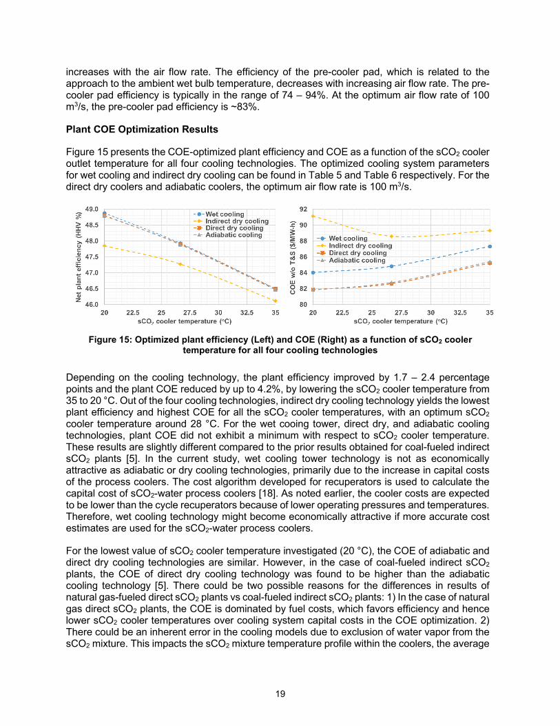
Figure 15 presents the COE-optimized plant efficiency and COE as a function of the sCO2 cooler outlet temperature for all four cooling technologies. The optimized cooling system parameters for wet cooling and indirect dry cooling can be found in Table 5 and Table 6 respectively. For the direct dry coolers and adiabatic coolers, the optimum air flow rate is 100 m3/s.

Figure 15: Optimized plant efficiency (Left) and COE (Right) as a function of sCO2 cooler

temperature for all four cooling technologies

Depending on the cooling technology, the plant efficiency improved by 1.7 – 2.4 percentage points and the plant COE reduced by up to 4.2%, by lowering the sCO2 cooler temperature from 35 to 20 °C. Out of the four cooling technologies, indirect dry cooling technology yields the lowest plant efficiency and highest COE for all the sCO2 cooler temperatures, with an optimum sCO2 cooler temperature around 28 °C. For the wet cooing tower, direct dry, and adiabatic cooling technologies, plant COE did not exhibit a minimum with respect to sCO2 cooler temperature. These results are slightly different compared to the prior results obtained for coal-fueled indirect sCO2 plants [5]. In the current study, wet cooling tower technology is not as economically attractive as adiabatic or dry cooling technologies, primarily due to the increase in capital costs of the process coolers. The cost algorithm developed for recuperators is used to calculate the capital cost of sCO2-water process coolers [18]. As noted earlier, the cooler costs are expected to be lower than the cycle recuperators because of lower operating pressures and temperatures. Therefore, wet cooling technology might become economically attractive if more accurate cost estimates are used for the sCO2-water process coolers.

For the lowest value of sCO2 cooler temperature investigated (20 °C), the COE of adiabatic and direct dry cooling technologies are similar. However, in the case of coal-fueled indirect sCO2 plants, the COE of direct dry cooling technology was found to be higher than the adiabatic cooling technology [5]. There could be two possible reasons for the differences in results of natural gas-fueled direct sCO2 plants vs coal-fueled indirect sCO2 plants: 1) In the case of natural gas direct sCO2 plants, the COE is dominated by fuel costs, which favors efficiency and hence lower sCO2 cooler temperatures over cooling system capital costs in the COE optimization. 2) There could be an inherent error in the cooling models due to exclusion of water vapor from the sCO2 mixture. This impacts the sCO2 mixture temperature profile within the coolers, the average

20

driving force and consequently, the cooling system capital costs. However, the COE results in Figure 15 indicate that the adiabatic cooling technology might become economically attractive with further reduction in sCO2 cooler temperature.

An important point to note is that the optimized results presented here are valid only for the selected plant design and ambient conditions. In case of higher/lower design ambient temperatures, the COE and optimum sCO2 cooler temperatures will change accordingly for each of the cooling technologies.

CONCLUSIONS & FUTURE WORK

This paper describes the development of performance and cost spreadsheet models for four cooling technologies available to the sCO2 research community – wet cooling tower [6], indirect dry [7], direct dry [8] and adiabatic cooling [9]. These models were originally developed for indirect, or externally heated sCO2 power plants, but were modified in the present study to accommodate sCO2 mixtures for direct-fired sCO2 power plants. Each of the cooling technology models were applied to optimize the COE of a natural gas-fueled direct sCO2 power plant at several sCO2 cooler outlet temperatures. Sensitivity analyses were conducted with respect to optimization variables to identify the optimum cooling system operating parameters. These sensitivity analyses presented tradeoffs between plant efficiency and COE.

Finally, a comparative analysis of all four cooling technologies was conducted for sCO2 cooler outlet temperatures in the range of 20 – 35 °C. Depending on the cooling technology, the plant efficiency is shown to improve by 1.7 – 2.4 percentage points and the plant COE is reduced by up to 4.2%, by lowering sCO2 cooler outlet temperature from 35 to 20 °C. This highlights the importance of optimizing cooling systems for direct-fired sCO2 power plants. Further, the results indicate that direct cooling approaches seem to offer the lowest COE options for the direct-fired sCO2 plant and ambient conditions under consideration. Future work in this area will focus on optimizing cooling systems and plant’s COE as a function of plant site ambient conditions, including seasonal temperature variability. Future studies will also investigate sCO2 cooler temperatures < 20 °C as there is room for further COE improvement.

ACKNOWLEDGMENTS

The authors would like to thank Richard Dennis (NETL) for his project support. The authors also wish to thank Wally Shelton, Travis Shultz (NETL), and Mark Woods (KeyLogic) for their technical assistance and input. Finally, the authors would like to thank Guentner for providing the vendor data for the dry and adiabatic cooling technologies. The work was completed under DOE NETL Contract Number DE-FE000401.

REFERENCES

[1] R. J. Allam, M. R. Palmer, G. W. Brown Jr, J. Fetvedt, D. Freed, H. Nomoto, M. Itoh, N. Okita and C. Jones Jr, "High efficiency and low cost of electricity generation from fossil fuels while eliminating atmospheric emissions, including carbon dioxide," Energy Procedia, vol. 37, pp. 1135-1149, 2013.

[2] J. D. Laumb, M. J. Holmes, J. J. Stanislowski, X. Lu, B. Forrest and M. McGroddy, "Supercritical CO2 cycles for power production," Energy Procedia, vol. 114, pp. 573-580, 2017.

[3] C. White and N. Weiland, "Preliminary cost and performance results for a natural gas fired direct sCO2 power plant," in Proceedings of the 6th International Supercritical CO2 Power Cycles Symposium, Pittsburgh, PA, USA, 2018.

21

[4] N. Weiland and C. W. White, "Performance and Cost Assessment of a Natural Gas-Fueled Direct sCO2 Power Plant," 2019.

[5] S. R. Pidaparti, C. W. White, A. O'Connel, N. T. Weiland and others, "Cooling system cost and performance models for economic sCO2 plant optimization of cooling with respect to cold sCO2 temperature," in 3rd European Conference on Supercritical CO2 (sCO2) Power Systems 2019: 19th-20th September 2019.

[6] National Energy Technology Laboratory (NETL), "Wet Cooling Tower Cooling System Spreadsheet Model for sCO2," 2019. [Online]. Available: https://www.netl.doe.gov/energy-analysis/details?id=3864.

[7] National Energy Technology Laboratory (NETL), "Indirect Dry Cooling System Spreadsheet Model for sCO2," 2019. [Online]. Available: https://www.netl.doe.gov/energy-analysis/details?id=3865.

[8] National Energy Technology Laboratory (NETL), "Direct Dry Cooling System Spreadsheet Model for sCO2," 2019. [Online]. Available: https://www.netl.doe.gov/energy-analysis/details?id=3866.

[9] National Energy Technology Laboratory (NETL), "Adiabatic Cooling System Spreadsheet Model for sCO2," 2019. [Online]. Available: https://www.netl.doe.gov/energy-analysis/details?id=3867.

[10] S. R. Pidaparti, C. W. White, A. C. O'Connell and N. T. Weiland, "Cooling Technology Models for Indirect sCO2 Cycles," NETL, Pittsburgh, 2019. [Online]. Available: https://netl.doe.gov/energy-analysis/details?id=3199

[11] National Energy Technology Laboratory (NETL), "Quality Guidelines for Energy System Studies - CO2 Impurity Design Parameters," Pittsburgh, Pennsylvania, August 2013.

[12] C. W. White and N. T. Weiland, "Evaluation of Property Methods for Modeling Direct-Supercritical CO2 Power Cycles," Journal of Engineering for Gas Turbines and Power, vol. 140, p. 011701, 2018.

[13] International Energy Agency Greenhouse Gas (IEAGHG), "Oxy-combustion Turbine Power Plants," Cheltenham, United Kingdom, August 2015.

[14] National Energy Technology Laboratory (NETL), "Quality Guidelines for Energy System Studies -- Capital Cost," NETL, Pittsburgh, January 2013.

[15] National Energy Technology Laboratory (NETL), "Quality Guidelines for Energy System Studies, Cost Estimation Methodology for NETL Assessments of Power Plant Performance," NETL, Pittsburgh, January 2013.

[16] N. Weiland, W. Shelton, T. Shultz, C. W. White and D. Gray, "Performance and Cost Assessment of a Coal Gasification Power Plant Integrated with a Direct-Fired sCO2 Brayton Cycle," 2017.

[17] T. Fout, A. Zoelle, D. Keairns, M. Turner, M. Woods, N. Kuehn, V. Shah, V. Chou and L. Pinkerton, "Cost and performance baseline for fossil energy plants volume 1a: bituminous coal (PC) and natural gas to electricity revision 3," US Department of Energy, Pittsburgh, PA, Report No. DOE/NETL-2015/1723, 2015.

[18] N. T. Weiland, B. W. Lance and S. R. Pidaparti, "sCO2 Power Cycle Component Cost Correlations From DOE Data Spanning Multiple Scales and Applications," in ASME Turbo Expo 2019: Turbomachinery Technical Conference and Exposition, 2019.

[19] E. W. Lemmon, I. H. Bell, M. L. Huber and M. O. McLinden, NIST Standard Reference Database 23: Reference Fluid Thermodynamic and Transport Properties-REFPROP, Version 10.0, National Institute of Standards and Technology, 2018.

[20] A. Zanker, Estimating cooling tower costs from operating data, vol. 79, MCGRAW HILL INC 1221 AVENUE OF THE AMERICAS, NEW YORK, NY 10020, 1972, p. 118.

[21] Chemical Engineering , "The Chemical Engineering Plant Cost Index," 2019. [Online]. Available: https://www.chemengonline.com/pci-home.

[22] National Energy Technology Laboratory (NETL), "Quality Guidelines for Energy System Studies -- Process Modeling Design Parameters," Pittsburgh, Pennsylvania, May, 2014.

[23] D. G. Kröger, Air-cooled heat exchangers and cooling towers, vol. 1, PennWell Books, 2004. [24] National Energy Technology Laboratory (NETL), "Air Cooled Heat Exchanger (ACHE) Design Final

Presentation," Pittsburgh, PA, 2017.

22

[25] S. Filippini, G. Mariani, L. Perrotta and U. Merlo, "EMERITUS: The New Condenser/CO2 Gas Cooler/Dry Cooler that Minimizes Energy Consumption," in 7th Conference on Ammonia and CO2 Refrigeration Technologies, Ohrid, 2017.

[26] M. Belusko, R. Liddle, A. Alemu, E. Halawa and F. Bruno, "Performance Evaluation of a CO2 Refrigeration System Enhanced with a Dew Point Cooler," Energies, vol. 12, no. 6, 2019.

[27] S. He, Z. Guan, H. Gurgenci, K. Hooman, Y. Lu and A. M. Alkhedhair, "Experimental study of film media used for evaporative pre-cooling of air," Energy conversion and management, vol. 87, pp. 874-884, 2014.

[28] SPX Cooling Technologies Inc., Cooling Tower Fundamentals 2nd Edition, Overland Park, Kansas, 2009.