Single machine scheduling to minimize total weighted tardiness

European Journal of Operational Research 165 (2005) 423–443

www.elsevier.com/locate/dsw

Single machine scheduling to minimize total weighted tardiness

T.C.E. Cheng a, C.T. Ng a,*, J.J. Yuan a,b, Z.H. Liu a,c

a Department of Logistics, The Hong Kong Polytechnic University, Hung Hom, Kowloon, Hong Kong, PR Chinab Department of Mathematics, Zhengzhou University, Zhengzhou, Henan 450052, PR China

c Department of Mathematics, East China University of Science and Technology, Shanghai 200237, PR China

Received 1 November 2002; accepted 1 September 2003

Available online 2 June 2004

Abstract

The problem of minimizing the total weighted tardiness in single machine scheduling is a well-known strongly NP-

hard problem. In this paper, we present an Oðn2Þ time approximation algorithm for the problem, where n is the number

of jobs. We further investigate different sub-models of the problem and obtain interesting properties and results. We

begin with the model where the job due dates are affine-linear functions of their processing times and the job tardiness

weights are proportional to their processing times. For this model, we classify the NP-hardness of the problem with

respect to different affine-linear functions, and provide an Oðn log nÞ algorithm for each of the polynomially solvable

problems. The second model we investigate is one where all job due dates have equal slacks, namely the SLK due-date

model. Results for this model include: the problem is NP-hard in the ordinary sense; a pseudo-polynomial algorithm

with time complexity Oðn2P Þ is derived, where P is the sum of all of the processing times; and a fully polynomial-time

approximation scheme is constructed.

� 2004 Elsevier B.V. All rights reserved.

Keywords: Single machine scheduling; Due dates; Tardiness; Processing-plus-wait; SLK due-dates

1. Introduction

We consider the single machine total weighted tardiness scheduling problem [3]. Let n jobs J1; J2; . . . ; Jnand a single machine that can handle only one job at a time be given. Each job Ji has a processing time pi, adue date di and a unit tardiness penalty wi. All jobs are available at time zero to be processed on the

machine without preemption. Let CiðpÞ and TiðpÞ ¼ maxf0;CiðpÞ � dig denote the completion time and

tardiness of job Ji respectively, under a job sequence p. For convenience, the job in position i under thesequence p will be denoted by JpðiÞ. The objective function to be minimized is the total weighted tardiness:

* Corresponding author. Tel.: +852-27667364; fax: +852-23302704.

E-mail addresses: [email protected] (T.C.E. Cheng), [email protected] (C.T. Ng), [email protected] (J.J. Yuan),

[email protected] (Z.H. Liu).

0377-2217/$ - see front matter � 2004 Elsevier B.V. All rights reserved.

doi:10.1016/j.ejor.2004.04.013

mailto:[email protected]

424 T.C.E. Cheng et al. / European Journal of Operational Research 165 (2005) 423–443

f ðpÞ ¼Xni¼1

wiTiðpÞ ¼Xni¼1

wpðiÞTpðiÞ:

The problem is to determine an optimal sequence p� that minimizes the function f ðpÞ. It is clear that no idle

time exists in the optimal sequence and so the processing of all jobs finishes at time P �Pn

i¼1 pi. As in [16],

we denote the problem as

1Xni¼1

wiTi

�� :

Although this problem of minimizing the total weighted tardiness on a single machine occurs frequently

in practice, only a few results involving arbitrary due dates and arbitrary weights have been reported in theliterature. Lawler [14] and Lenstra et al. [16] prove that the problem 1k

Pni¼1 wiTi is strongly NP-hard. Potts

and Van Wassenhove [19] give a branch-and-bound algorithm for this problem. Schrage and Baker [20]

give an Oð2nÞ dynamic programming algorithm to solve this and other scheduling problems. Abdul-Razaq

et al. [1] give a survey of dynamic programming algorithms and branch-and-bound algorithms for this

problem. Since the dynamic programming approach requires Oð2nÞ time and the branch-and-bound ap-

proach may require complete enumeration of all possible solutions in the worst case, a more efficient

algorithm has been desired for a long time. To this end, we provide in this paper an Oðn2Þ time approxi-

mation algorithm for this problem.Since problems with arbitrary due dates are quite hard to handle analytically, interest in special due date

models has been increasing lately. For example, the common/constant (CON) due date model, i.e., di ¼ d,where a common/constant due date is assigned to all jobs, has been widely studied. For this model, Yuan

[23] shows that the problem 1jdi ¼ djPn

i¼1 wiTi is NP-hard in the ordinary sense. Lawler and Moore [15]

provide a pseudo-polynomial algorithm for the problem 1jdi ¼ djPn

i¼1 wiTi, and show that the problem

1jdi ¼ djPn

i¼1 Ti is polynomially solvable. Another widely studied due date model is the equal-slack (SLK)

due date model, i.e., di ¼ pi þ q, where q is a given constant. Lawler [14] shows that the problem

1jdi ¼ pi þ qjPn

i¼1 Ti is polynomially solvable. Other scheduling studies involving the SLK due dates can befound in [4–6,17]. A more general due date model is one in which the due dates are affine-linear functions of

the job processing times, i.e., di ¼ api þ q, where a and q are given constants. This model is called the

processing-plus-wait (PPW) due date model (see Kahlbacher and Cheng [12] and Cheng and Kovalyov [7]).

The rationale of the PPW due date model is based on the observation that the due date of a job is pro-

portional to its processing time in many practical situations. The PPW due dates were probably first

introduced by Smith and Seidmann [21], where the model was called total work and number of operations

(TWNO). Since in a single-machine environment each job consists of a single operation, the TWNO due

dates become the PPW due dates in single machine systems. A review of research on due date assignmentand scheduling is given in Cheng and Gupta [5].

Besides special due date models, researchers are also interested in models where special restrictions are

imposed on other problem parameters. For example, Du and Leung [8] prove that the problem

1jwi ¼ 1jPn

i¼1 wiTi is NP-hard in the ordinary sense, and Lawler [14] gives a pseudo-polynomial algorithm

for this problem. Arkin and Roundy [2] show that the problem 1jwi ¼ kpijPn

i¼1 wiTi, where k is a constant,

is also NP-hard in the ordinary sense, and give a pseudo-polynomial algorithm for this problem. Similarly,

Lenstra et al. [16] show that the problem 1jpi ¼ pjPn

i¼1 wiTi is polynomially solvable.

As seen from the above, the research trend is moving towards studying special models of the generaltotal weighted tardiness problem. We follow this trend in this present study where we will consider different

special models of the problem. To the best of our knowledge, there is no report on the models: (A)

1jdi ¼ api þ q, wi ¼ kpijPn

i¼1 wiTi, and (B) 1jdi ¼ pi þ qjPn

i¼1 wiTi in the literature. We attempt to fill these

gaps in this paper. The results we have obtained for these two models can be summarized as follows.

T.C.E. Cheng et al. / European Journal of Operational Research 165 (2005) 423–443 425

For model (A), we classify its NP-hardness with respect to different values of a. The results are:

1. If 0 < a < 1, then the problem is NP-hard in the ordinary sense. A pseudo-polynomial algorithm for this

problem can be found in [2].

2. If a6 0, then the problem is solved by the longest processing time (LPT) rule.

3. If aP 1, then the problem is solved by the shortest processing time (SPT) rule.

For model (B), the results include:

1. The problem is NP-hard in the ordinary sense.

2. A pseudo-polynomial algorithm with time complexity Oðn2P Þ is derived.3. A fully polynomial-time approximation scheme, discussed below, is obtained.

Suppose that we are considering an NP-hard optimization problem. Let q be a number with q > 1. A q-approximation algorithm [10] is a polynomial-time algorithm that always finds a solution having an

objective function value within a factor of q of the optimal. We say that a family of algorithms fHeg is a

polynomial-time approximation scheme (PTAS) [10] for an optimization problem A, if for every e > 0, He isa ð1þ eÞ-approximation algorithm for A. Furthermore, if for every e > 0, He is a (1þ e)-approximation

algorithm for A with a time requirement which is polynomial in the size of A and 1e, then we say that fHeg is

a fully polynomial-time approximation scheme (FPTAS) [10] for A.The following is a practical example of model (A): A building contractor has been awarded a contract to

build apartments of different designs at n different sites, i.e., n jobs, for a property developer. Since the core

building equipment such as tower cranes, elevators, excavators and bulldozers, etc., is very expensive, the

contractor does not own this equipment in order to reduce the costs and risks. Instead, on landing the

contract, the contractor will hire the necessary equipment for each individual site from equipment suppliers.Each site will be managed by a project management team comprising experienced management and engi-

neering personnel from the contractor. Due to the scarce human and equipment resources, the contractor

can only work on one site at a time. Since a site of complicated apartments will take a longer time to process,

a longer due date will be allowed for its construction. A reasonable way to set the due date is di ¼ api þ q,which relates the due date of a job to its processing time proportionally. It is a practice in the construction

industry that contractors are charged penalties for failing to complete jobs on time. The penalty is pro-

portional to the value of the job and its tardiness. So, for each site of apartments completed tardy, the

contractor is liable to a penalty Pi ¼ wiTi, where wi is the tardiness weight, i.e., the unit tardiness penalty,which is proportional to the job’s value and Ti is the amount of tardiness incurred. Since a site comprising

more complicated apartments normally commands a higher value and it takes a longer time to construct, it is

reasonable to assume that the tardiness weight is proportional to its processing time, i.e., wi ¼ kpi.In model (B), the due date assignment method is a special case of the PPW due date assignment method

for which a ¼ 1 and there is no restriction on the tardiness weight wi. Therefore, examples valid for model

(A) are also valid for model (B) with no restriction on wi.

The rest of this paper is organized as follows. The Oðn2Þ time approximation algorithm for the general

problem 1kPn

i¼1 wiTi will be given in Section 2. In Section 3, we consider the problem model (A)1jdi ¼ api þ q, wi ¼ kpij

Pni¼1 wiTi and classify its NP-hardness according to different values of a. The

problem model (B) 1jdi ¼ pi þ qjPn

i¼1 wiTi is considered in Section 4. We present some preliminary results

in Section 4.1. Then, we prove that the problem 1jdi ¼ pi þ qjPn

i¼1 wiTi is NP-hard in Section 4.2. A

pseudo-polynomial algorithm for the problem 1jdi ¼ pi þ qjPn

i¼1 wiTi with time complexity Oðn2P

piÞ is

derived in Section 4.3. Based on the polynomial-time approximation algorithm obtained in Section 2, we

modify the pseudo-polynomial algorithm to derive an FPTAS for this problem in the later part of Section

4.3. Finally, some concluding remarks are given in Section 5.


2. A polynomial-time approximation algorithm for the general total weighted tardiness problem

Several heuristics are proposed in the literature for the general total weighted tardiness problem

1kPn

i¼1 wiTi, and experimental results for these heuristics are presented (see [11,22] for example). Up to

now, no performance ratio of these heuristics has been analyzed from a theoretical point of view. In

contrast, we give, in this section, a polynomial-time ðn� 1Þ-approximation algorithm for the problem

1kPn

i¼1 wiTi. This approximation algorithm will also be used in Section 4.3 where an upper bound for the

optimal objective value of the problem 1jdi ¼ pi þ qjPn

i¼1 wiTi will be constructed.We recall that Lawler [13] first gives an algorithm that solves the problem 1kmax16 i6 n wiTi in Oðn2Þ

time. This algorithm will be called Lawler’s algorithm.

Our approximation algorithm, which we call ‘‘Modified Lawler’s Algorithm’’, for the general total

weighted tardiness problem 1kPn

i¼1 wiTi can be described as follows.

For n jobs J1; J2; . . . ; Jn with processing times p1; p2; . . . ; pn, due-dates d1; d2; . . . ; dn and weights

w1;w2; . . . ;wn, respectively, we first compute the modified due-date d 0i ¼ maxfpi; dig for each job Ji,

16 i6 n, where the notion of modified due-dates was first described by Lawler in [14]. Then, by Lawler’s

algorithm, we construct the schedule p� that minimizes the objective function gðpÞ ¼ max16 i6 n wiT 0i ðpÞ,

where T 0i ðpÞ ¼ maxf0;CiðpÞ � d 0

ig, is the tardiness of job Ji under the sequence p with respect to the

modified due-date d 0i . The sequence p� is an approximate solution.

Modified Lawler’s Algorithm

Step 1. Modify the due-dates by setting

d 0i ¼ maxfpi; dig; 16 i6 n:

Step 2. Set k :¼ n, J :¼ fJ1; J2; . . . ; Jng and P :¼Pn

i¼1 pi.Step 3. Pick Jj 2 J such that wj �maxf0; P � d 0

jg is minimum among wi �maxf0; P � d 0ig, Ji 2 J and

then set p�ðkÞ ¼ j.Step 4. Set k :¼ k � 1, J :¼ J n fJjg and P :¼ P � pj.Step 5. If k ¼ 0 then stop. Otherwise, return to Step 3.

Theorem 2.1. The Modified Lawler’s Algorithm is an ðn� 1Þ-approximation algorithm with time complexitybounded above by Oðn2Þ for the general total weighted tardiness problem 1k

Pni¼1 wiTi.

Proof. Computing d 0i , i ¼ 1; . . . ; n takes OðnÞ time. Finding the sequence p� by Lawler’s algorithm takes

Oðn2Þ time. Therefore, the time complexity of Modified Lawler’s Algorithm is Oðn2Þ. Let

f ðrÞ ¼Pn

i¼1 wiTiðrÞ and f 0ðrÞ ¼Pn

i¼1 ¼ wiT 0i ðrÞ. Then, for any r,

gðrÞ ¼ max16 i6 n

wiT 0i ðrÞ6

Xni¼1

wiT 0i ðrÞ ¼ f 0ðrÞ:

If pi < di, then d 0i ¼ di and TiðrÞ � T 0

i ðrÞ ¼ 0. If pi P di, then d 0i ¼ pi and, by noting that CiðrÞP pi P di,

TiðrÞ � T 0i ðrÞ ¼ maxf0;CiðrÞ � dig �maxf0;CiðrÞ � pig ¼ pi � di. Thus, TiðrÞ � T 0

i ðrÞ ¼ maxf0; pi � dig.Therefore, we have

f 0ðrÞ ¼ f ðrÞ �Xni¼1

wi½TiðrÞ � T 0i ðrÞ� ¼ f ðrÞ �

Xni¼1

wi maxf0; pi � dig:

Let r� be the sequence that minimizes f ðrÞ. Since p� minimizes gðpÞ, we have that gðp�Þ6 gðr�Þ. Note

that d 0i P pi for each i. Therefore, the first job under any sequence has zero tardiness with respect to its

modified due date. It holds that


f 0ðp�Þ6 ðn� 1Þgðp�Þ6 ðn� 1Þgðr�Þ6 ðn� 1Þf 0ðr�Þ:

Hence, we have

f ðp�Þ �Xni¼1

wi maxf0; pi � dig6 ðn� 1Þ f ðr�Þ �Xni¼1

wi maxf0; pi � dig !

:

Then, f ðp�Þ6 ðn� 1Þf ðr�Þ. The result follows. h

The following instance shows that the bound n� 1 in Theorem 2.1 is asymptotically tight. Let

p1 ¼ p2 ¼ m3; and pi ¼ m; for i ¼ 3; 4; . . . ; n;

d1 ¼ d2 ¼ m3; and di ¼ m3 þ ði� 2Þm; for i ¼ 3; 4; . . . ; n;

w1 ¼ 1; for i ¼ 1; 2; . . . ; n:

One can verify that Modified Lawler’s Algorithm generates the sequence p� ¼ ð1; 2; . . . ; nÞ with

f ðp�Þ ¼ ðn� 1Þm3. However, the optimal sequence r� ¼ ð1; 3; 4; . . . ; n; 2Þ has f ðr�Þ ¼ m3 þ ðn� 2Þm. Thus,f ðp�Þ=f ðr�Þ tends to n� 1 as m ! þ1.

3. Problem model (A)

In this section we investigate the problem model 1jdi ¼ api þ q, wi ¼ kpijPn

i¼1 wiTi. We will classify

different cases of the problem as NP-hard or not according to different values of a, and give algorithms for

the polynomially solvable cases.

3.1. NP-hard case

We use the well-known 2-Partition problem for the NP-hardness reduction.2-Partition problem: Given a set of t different positive integers A ¼ fa1; a2; . . . ; atg such that

Pti¼1 ai ¼ 2B

is even, is there a partition of A into A1 and A2 such thatP

ai2A1ai ¼

Pai2A2

ai ¼ B?

Lemma 3.1.1 [9]. The 2-Partition problem is NP-complete in the ordinary sense.

We will prove that the problem 1jdi ¼ api þ q, wi ¼ kpijPn

i¼1 wiTi is NP-hard for 0 < a < 1 by showing

that the corresponding decision problem is NP-complete. Our reduction is a modification of the one in [2].

Theorem 3.1.2. The problem

1jdi ¼ api þ q; wi ¼ kpijXni¼1

wiTi

is NP-hard for every fixed a with 0 < a < 1.

Proof. The decision version of our problem is clearly in the class NP.

For a given instance of the 2-Partition problem: a1; a2; . . . ; at with 12

Pti¼1 ai ¼ B, we can suppose that

BP maxf1a ; 11�ag, for otherwise, each ai can be replaced by mai, where m is a sufficiently large number. We

construct an instance of our decision problem as follows:


n ¼ t þ 1;

wi ¼ pi ¼ ai; for 16 i6 t;

wn ¼ pn ¼ 4B3;

q ¼ 4B3ð1� aÞ þ B;

Y ¼ 4B4aþ B2:

The reduction can be done in polynomial time. We show in the sequel that the instance of the 2-Partition

problem has a solution if and only if the instance of the decision version of our problem has a sequence psuch that f ðpÞ6 Y .

For a sequence p of the above instance, set

JE ¼ fJijJi is processed before Jn under pg;

JL ¼ fJijJi is processed after Jn under pg:
The relative positions are shown in Fig. 1.
Because BP maxf1a ; 11�ag, we have

q ¼ 4B3ð1� aÞ þ BP 4B2 þ B > 2B ¼Xt

i¼1

pi;

and

q ¼ 4B3 � 4B3aþ B6 4B3 � 4B2 þ B < 4B3 ¼ pn:

Then Cj < q6 dj for Jj 2 JE, and Cj > Cn þ pj > qþ pj P dj for Jj 2 JL. It follows that the jobs in JE are all

on time and the jobs in JL are all tardy. Let

PE ¼XJi2JE

pi and PL ¼XJi2JL

pi:

For a job Ji 2 JL, set

JLðiÞ ¼ fJj 2 JLjJj is processed before Ji under pg:
Because CnðpÞ ¼ PE þ pn and
CiðpÞ ¼ PE þ pn þX

Jj2JLðiÞpj þ pi for Ji 2 JL;

i.e.,

CiðpÞ ¼ PE þX

Jj2JLðiÞpj þ pi þ qþ ð4B3a� BÞ; for Ji 2 JL;

we have

TnðpÞ ¼ maxf0; PE � Bg;

Fig. 1.


TiðpÞ ¼ PE þX

Jj2JLðiÞpj þ ð1� aÞpi þ ð4B3a� BÞ; for Ji 2 JL:

Since
XJi2JL
piX

Jj2JLðiÞpj þ

1

2

XJi2JL

p2i ¼1

2P 2L ;

it follows that the sum of the tardiness penalties is

f ðpÞ ¼ pnTn þXJi2JL

piTi ¼ pn maxf0; PE � Bg þXJi2JL

pi PE

0@ þ

XJj2JLðiÞ

pj þ ð1� aÞpi þ 4B3a� B

1A

¼ 4B3 maxf0; PE � Bg þ ð2B� PLÞPL þ1

2P 2L þ

XJi2JL

1

2

�� a

�p2i þ ð4B3a� BÞPL

¼ 4B3 maxf0; PE � Bg þ ð4B3aþ BÞPL �1

2P 2L þ

XJi2JL

1

2

�� a

�p2i :

Notice that

1

2P 2L �

XJi2JL

1

2

�� a

�p2i < P 2

L 6 4B2;

so we also have

f ðpÞ > 4B3 maxf0; PE � Bg þ ð4B3aþ BÞPL � 4B2:

Because pi ¼ ai (for 16 i6 t), we only need to prove in the following that f ðpÞ6 Y if and only if PL ¼ B.If PL ¼ B, then PE ¼ B. Because

� 1

2P 2L þ

XJi2JL

1

2

�� a

�p2i 6 0;

we have

f ðpÞ6 ð4B3aþ BÞPL ¼ 4B4aþ B2 ¼ Y :

If PL > B, then PE < B. Set PL ¼ Bþ x, where xP 1, then

f ðpÞ > ð4B3aþ BÞPL � 4B2 ¼ Y þ ð4B3aþ BÞx� 4B2:

For the reason that BaP 1, we have

ð4B3aþ BÞxP 4B3aþ BP 4B2 þ B > 4B2:

Thus, we deduce that f ðpÞ > Y .If PL < B, then PE > B. Set PE ¼ Bþ h, where hP 1, then PL ¼ B� h and

f ðpÞ > 4B3hþ ð4B3aþ BÞðB� hÞ � 4B2 ¼ Y þ ð4B3ð1� aÞ þ BÞh� 4B2:

For the reason that Bð1� aÞP 1, we have

ð4B3ð1� aÞ þ BÞhP 4B3ð1� aÞ þ BP 4B2 þ B > 4B2:

Then, we deduce that f ðpÞ > Y . This completes the proof. h

The question of whether the problem 1jdi ¼ api þ qjPn

i¼1 wiTi is strongly NP-hard is still open.


3.2. Polynomially solvable cases

Now, we will give two polynomially solvable cases of the problem 1jdi ¼ api þ q, wi ¼ kpijPn

i¼1 wiTi.We first consider the following two results.

Theorem 3.2.1. Suppose that a is a rational number with a6 0. If p1 P p2 P � � � P pn and w1=p1 Pw2=p2 P � � � Pwn=pn, then the sequence ð1; 2; . . . ; nÞ is optimal for the problem 1jdi ¼ api þ qj

Pni¼1 wiTi.

Proof. The proof is by Adjacent Pairwise Interchange. Suppose that in a sequence p, job Jj comes imme-

diately before job Ji where i < j. We claim that the sequence p� obtained from p by interchanging the

positions of jobs Ji and Jj is not worse than p. Recall that Rþ ¼ maxf0;Rg for any real number R. LetX ¼ CiðpÞ � q. Then,

TiðpÞ ¼ ðX � apiÞþ; TjðpÞ ¼ ðX � pi � apjÞþ;

Tiðp�Þ ¼ ðX � pj � apiÞþ; Tjðp�Þ ¼ ðX � apjÞþ:

Therefore, our claim is equivalent to

wiðX � apiÞþ þ wjðX � pi � apjÞþ PwiðX � pj � apiÞþ þ wjðX � apjÞþ: ð1Þ

For any real numbers Y , a and b with bP 0, we define ga;bðY Þ ¼ ðY � aÞþ � ðY � a� bÞþ. From this

definition, we get

ga;bðY Þ ¼ minfðY � aÞþ; bgP 0: ð2Þ

To show (1), it suffices to show that

wigapi;pjðX ÞPwjgapj;piðX Þ; for all X :

By (2), we have

pigapi;pjðX Þ ¼ minfpiðX � apiÞþ; pipjg;

and

pjgapj;piðX Þ ¼ minfpjðX � apjÞþ; pipjg:

Since a6 0 and pi P pj, we have X � api PX � apj, and so ðX � apiÞþ P ðX � apjÞþ. Then,

piðX � apiÞþ P pjðX � apjÞþ;

and, therefore,

minfpiðX � apiÞþ; pipjgP minfpjðX � apjÞþ; pipjg:

That is, pigapi;pjðX ÞP pjgapj;piðX Þ. Since wi=pi Pwj=pj, we obtain

wigapi;pjðX Þ ¼ ðwi=piÞpigapi;pjðX ÞP ðwj=pjÞpjgapj;piðX Þ ¼ wjgapj;piðX Þ; for all X : �


Remark for Theorem 3.2.1. The pairwise-job interchange method does not work for the case where

p1 P p2 P � � � P pn and w1 Pw2 P � � � Pwn. In fact, it is implied in [23] that even the problem

1jdi ¼ qjPn

i¼1 wiTi is NP-hard for this special case.

Similarly, we can prove the following theorem.

Theorem 3.2.2. Suppose that a is a number with a > 1. If p1 6 p2 6 � � � 6 pn and w1=p1 Pw2=p2 P � � � Pwn=pn, then the sequence p ¼ ð1; 2; . . . ; nÞ is optimal for the problem 1jdi ¼ api þ qj

Pni¼1 wiTi.

As a consequence of Theorems 3.2.1 and 3.2.2, we have the following corollary.

Corollary 3.2.3. For the problem 1jdi ¼ api þ q, wi ¼ kpijPn

i¼1 wiTi, if a6 0, it can be solved by the LPT rule;if aP 1, it can be solved by the SPT rule.

4. Problem model (B)

In this section, we will investigate the problem model 1jdi ¼ pi þ qjPn

i¼1 wiTi.

4.1. Some preliminary results

We first give some simple properties for the problem 1jdi ¼ pi þ qjPn

i¼1 wiTi. These properties are key to

the rest of this section.

Lemma 4.1.1. For any given sequence p for the problem 1jdi ¼ pi þ qjPn

i¼1 wiTi, if JpðlÞ is a tardy job, theneach job JpðiÞ with l6 i6 n is tardy and

i�1

TpðiÞ ¼ TpðlÞ þXj¼l

ppðjÞ:

Proof. Note that CpðlÞ ¼ TpðlÞ þ dpðlÞ ¼ TpðlÞ þ ppðlÞ þ q ¼ TpðlÞ þ ppðlÞ � ppðiÞ þ dpðiÞ. Thus,

CpðiÞ ¼ CpðlÞ þXi

j¼lþ1

ppðjÞ ¼ TpðlÞ þXi�1

j¼l

ppðjÞ þ dpðiÞ:

The result follows. h

Lemma 4.1.2. For any given sequence p for the problem 1jdi ¼ pi þ qjPn

i¼1 wiTi, let Jpði0Þ be the first tardy job.Then, the objective function f ðpÞ can be re-written as

f ðpÞ ¼ Tpði0ÞXni¼i0

wpðiÞ þX

i0 6 i<j6 n

ppðiÞwpðjÞ:

Proof. Since job Jpði0Þ is the first tardy job under p, we have f ðpÞ ¼Pn

i¼i0wpðiÞTpðiÞ. By Lemma 4.1.1,

TpðiÞ ¼ Tpði0Þ þPi�1

j¼i0ppðjÞ for i0 6 i6 n. Therefore,

f ðpÞ ¼ Tpði0ÞXni¼i0

wpðiÞ þXni¼i0

Xi�1

j¼i0

wpðiÞppðjÞ ¼ Tpði0ÞXni¼i0

wpðiÞ þX

i0 6 i<j6 n

ppðiÞwpðjÞ: �


Lemma 4.1.3. Let JpðlÞ be a tardy job in a given sequence p for the problem 1jdi ¼ pi þ qjPn

i¼1 wiTi.Then,

TpðlÞ þX

l6 i6 n

ppðiÞ ¼Xni¼1

ppðiÞ � q:

Proof. It is a direct consequence of the definition of Ti as it is clear that no idle time exists in an optimal

sequence. h

The following are some inequalities that will be used later in this section.

Lemma 4.1.4. Let l1; l2; . . . ; ln be positive integers with L ¼Pn

i¼1 li. Suppose that F is a positive number.Then,

(i) 0 <P

16 i<j6 n lilj <12L2,

(ii)P

16 i<j6 n ðF þ liÞðF þ ljÞ > 12nðn� 1ÞF 2 þ ðn� 1ÞFL, and

(iii)P

16 i<j6 n ðF þ liÞðF þ ljÞ < 12nðn� 1ÞF 2 þ ðn� 1ÞFLþ 1

2L2.

Proof. (i) is a fundamental result in algebra. To prove (ii) and (iii), we observe that
X16 i<j6 n
ðF þ liÞðF þ ljÞ ¼1

2nðn� 1ÞF 2 þ

X16 i<j6 n

ðli þ ljÞF þX

16 i<j6 n

lilj:

By symmetry,

X16 i<j6 n

ðli þ ljÞ ¼1

2

Xi6¼j

ðli þ ljÞ ¼1

2

Xni¼1

Xnj¼1

ðli þ ljÞ �Xni¼1

li ¼ ðn� 1ÞL:

Therefore,

X16 i<j6 n

ðF þ liÞðF þ ljÞ ¼1

2nðn� 1ÞF 2 þ ðn� 1ÞFLþ

X16 i<j6 n

lilj:

Combining the last equation with (i), we obtain (ii) and (iii). h

The following is the well-known Equal Size 2-Partition problem, which will be used to prove the NP-

hardness of the problem.

Equal Size 2-Partition problem: Given 2t positive integers a1; a2; . . . ; a2t such thatP2t

i¼1 ai ¼ 2B is even,

is there a partition of A ¼ f1; 2; . . . ; 2tg into A1 and A2 such that jA1j ¼ jA2j ¼ t andP

i2A1ai ¼

Pi2A2

ai¼ B?

Lemma 4.1.5 ([9]). The Equal Size 2-Partition problem is NP-complete in the ordinary sense.

4.2. An NP-hardness proof

We will prove that the problem


1jdi ¼ pi þ qXni¼1

wiTi

��
is NP-hard in the ordinary sense by showing that the corresponding decision problem is NP-complete in the
ordinary sense.

Theorem 4.2.1. The problem 1 di ¼ pi þ qj jPn

i¼1 wiTi is NP-hard in the ordinary sense.

Proof. The decision version of our problem is clearly in the class NP.

For a given instance of the Equal Size 2-Partition problem: a1; a2; . . . ; a2t with 12

P2ti¼1 ai ¼ B (without loss

of generality, we suppose tP 2 in the sequel), we construct an instance of our decision problem as follows:

n ¼ 2t þ 1;

y ¼ 2tð3t � 1ÞB6 þ 4ð3t � 1ÞB4 þ 6B2;

pi ¼ wi ¼ 2B3 þ 2ai; 16 i6 2t;

pn ¼ 2tB3 þ 2B and wn ¼ y þ 1;

di ¼ pi þ 2tB3 þ 2B ðor equivalently q ¼ 2tB3 þ 2BÞ; 16 i6 n:

The reduction can be done in polynomial time. We show in the sequel that the instance of the Equal Size

2-Partition problem has a solution if and only if the instance of the decision version of our problem has a

sequence p such that f ðpÞ6 y.If the Equal Size 2-Partition problem has a solution, then there is a partition of A ¼ f1; 2; . . . ; 2tg into A1

and A2 such that jA1j ¼ jA2j ¼ t andP

i2A1ai ¼

Pi2A2

ai ¼ B. As shown in Fig. 2, we define a job sequence pwhich satisfies the following conditions:

fpðiÞj16 i6 tg ¼ A1;

pðt þ 1Þ ¼ n;

fpðiÞjt þ 26 i6 ng ¼ A2:

Because

Xt

i¼1

ppðiÞ ¼Xni¼tþ2

ppðiÞ ¼ 2tB3 þ 2B;

Jpðtþ1Þ ¼ Jn is the last on-time job under the sequence p with

Cpðtþ1Þ ¼ dpðtþ1Þ ¼ 4tB3 þ 4B;

and so

Tpðtþ2Þ ¼ Cpðtþ1Þ � q ¼ 2tB3 þ 2B:

Fig. 2.


Hence, by Lemma 4.1.2, we have

f ðpÞ ¼ Tpðtþ2ÞXni¼tþ2

wpðiÞ þX

tþ26 i<j6 n

ppðiÞwpðjÞ

¼ ð2tB3 þ 2BÞð2tB3 þ 2BÞ þX

tþ26 i<j6 n

ð2B3 þ 2apðiÞÞð2B3 þ 2apðjÞÞ:

According to Lemma 4.1.4, we have

Xtþ26 i<j6 n

ð2B3 þ 2apðiÞÞð2B3 þ 2apðjÞÞ6 2tðt � 1ÞB6 þ 4ðt � 1ÞB4 þ 2B2:

Thus, we have

f ðpÞ6 2tð3t � 1ÞB6 þ 4ð3t � 1ÞB4 þ 6B2 ¼ y;

and so p is a required sequence for our problem.

Now suppose that the instance of the Equal Size 2-Partition problem has no solution. We only need to

prove that f ðpÞ > y for any job sequence p. The special structure of pi implies the following claim.

Claim 1. There is no subset S � fJ1; J2; . . . ; J2tg such thatP

Ji2S pi ¼ q ¼ 2tB3 þ 2B.Suppose that p is any given sequence. Let m be the integer such that pðmÞ ¼ n, i.e., JpðmÞ ¼ Jn.If Jn is tardy under p, then f ðpÞ > y is implied by the fact wn ¼ y þ 1.

We suppose that Jn is on time under p. We first prove the following claim.Claim 2. m6 t þ 1.

Otherwise, mP t þ 2. By the fact that pi > 2B3, we deduce

Xm�1

i¼1

ppðiÞ PXtþ1

i¼1

ppðiÞ > 2ðt þ 1ÞB3 > q:

Hence, we get TpðmÞ > 0 and Jn is tardy under p, a contradiction. This completes the proof of Claim 2.By using Claim 2, we only need to consider the following two cases.

Case 1. m6 t.In this case, Jpðtþ1Þ is a tardy job under p. By using Lemma 4.1.3, we deduce

Tpðtþ1Þ þXni¼tþ1


and so


2apðiÞ ¼ 2ðt � 1ÞB3 þ 4B:

Because

Tpðtþ1Þ þX

16 i6 t;i6¼m

ppðiÞ > 2ðt � 1ÞB3;

by using Lemma 4.1.4, we have


f ðpÞP Tpðtþ1ÞXni¼tþ1

wpðiÞ þX

tþ16 i<j6 n

ppðiÞwpðjÞ

¼ Tpðtþ1Þ 2ðt

þ 1ÞB3 þXni¼tþ1

2apðiÞ

!þ

Xtþ16 i<j6 n

2B3�

þ 2apðiÞ�2B3�

þ 2apðjÞ�

> 2ðt þ 1ÞB3Tpðtþ1Þ þX

tþ16 i<j6 n

ð2B3 þ 2apðiÞÞð2B3 þ 2apðjÞÞ

> 2ðt þ 1ÞB3Tpðtþ1Þ þ 2tðt þ 1ÞB6 þ 2tB3Xni¼tþ1

2apðiÞ

¼ 2B3Tpðtþ1Þ þ 2tðt þ 1ÞB6 þ 2tB3 Tpðtþ1Þ

þXni¼tþ1

2apðiÞ

!

> 4ðt � 1ÞB6 þ 2tðt þ 1ÞB6 þ 2tB3ð2ðt � 1ÞB3 þ 4BÞ

¼ ð6t2 þ 2t � 4ÞB6 þ 8tB4 > y:

Case 2. m ¼ t þ 1.

In this case, Jpðtþ2Þ is the first tardy job under p. By using Lemma 4.1.3, we deduce



and so


2apðiÞ ¼ 2tB3 þ 4B:

Because JpðmÞ ¼ Jn is on time, we deduce by Claim 1 that

Xt

i¼1

ppðiÞ < q ¼ 2tB3 þ 2B:

This implies thatPt

i¼1 2apðiÞ < 2B, and so

Xni¼tþ2

apðiÞ PBþ 1:

We write x ¼Pn

i¼tþ2 2apðiÞ in the sequel. Then, we have

2Bþ 26 x < 4B;

and so

ð2ðt � 1ÞB3 þ 4B� xÞx > 4ðt � 1ÞB4 þ 4ðt � 1ÞB3:


By using Lemma 4.1.4, we have

f ðpÞP Tpðtþ2ÞXni¼tþ2

wpðiÞ þX

tþ26 i<j6 n

ppðiÞwpðjÞ

¼ Tpðtþ2Þð2tB3 þ xÞ þX

tþ26 i<j6 n

ð2B3 þ 2apðiÞÞð2B3 þ 2apðjÞÞ

> ð2tB3 þ 4B� xÞð2tB3 þ xÞ þ 2tðt � 1ÞB6 þ 2ðt � 1ÞB3x

¼ 2tð3t � 1ÞB6 þ 8tB4 þ ð2ðt � 1ÞB3 þ 4B� xÞx> 2tð3t � 1ÞB6 þ 4ð3t � 1ÞB4 þ 4ðt � 1ÞB3

¼ y þ 4ðt � 1ÞB3 � 6B2 > y:

This completes the proof. h

4.3. A pseudo-polynomial algorithm and a fully polynomial-time approximation scheme

We will first design a pseudo-polynomial algorithm to solve the problem 1jdi ¼ pi þ qjPn

i¼1 wiTi byimitating the algorithm for OPTIMIZATION 0–1 KNAPSACK in [18]. In the rest of this paper, we assume

that all the pi’s, wi’s and q are integers.

Note that di ¼ pi þ qP pi for all 16 i6 n. Thus, for any sequence p, job Jpð1Þ must be on time. Therefore,

the last on-time job must exist in any sequence. The following result, and Lemma 4.1.1, are critical to the

design of our pseudo-polynomial algorithm.

Lemma 4.3.1. There is an optimal sequence p for the scheduling problem with SLK due-dates

1 dij ¼ pi þ qjXni¼1

wiTi;

such that, if JpðlÞ is the first tardy job under p, then we have the following results:

(1)wpðlÞppðlÞ

P wpðlþ1Þppðlþ1Þ

P � � � P wpðnÞppðnÞ

.

(2) If there are two jobs JpðkÞ and JpðtÞ such that k; tP l andwpðkÞppðkÞ

¼ wpðtÞppðtÞ

, then the sequence p� obtained from p by

exchanging the positions of pðkÞ and pðtÞ is still optimal.(3) The first l� 2 on-time jobs can be scheduled in any order among themselves without affecting the optimal-

ity.(4) The last on-time job, i.e., job Jpðl�1Þ, is such that ppðl�1Þ ¼ max16 i6 l�1 ppðiÞ.

Proof. Let p be an optimal sequence for the considered problem. If JpðlÞ is the first tardy job under p, thenthe objective value can be denoted by

f ðpÞ ¼Xnj¼l

wpðjÞCpðjÞ �Xnj¼l

wpðjÞdpðjÞ:

Then, (1) and (2) can be established by the pairwise-job interchange method. Since jobs Jpð1Þ; Jpð2Þ; . . . ; Jpðl�1Þare on-time jobs, we have CpðiÞ 6 dpðiÞ, i.e., Cpði�1Þ 6 q, for i ¼ 1; . . . ; l� 1, where Cpð0Þ � 0. This is equivalentto Cpðl�2Þ 6 q. Therefore, rearranging the first l� 2 on-time jobs in any order will still keep these l� 2 jobs

on time. Hence, (3) follows.

In addition, since Cpðl�2Þ 6 q is equivalent to ppðl�1Þ PCpðl�1Þ � q, by exchanging job Jpðl�1Þ with the

largest job among the first l� 1 jobs will still keep the first l� 1 jobs on time. Therefore, (4) follows. �


Any sequence p satisfying conditions (1) and (4) of Lemma 4.3.1, where l is the least integer such thatCpðl�1Þ > q, is called a regular sequence. By Lemma 4.3.1, to solve the problem


wiTi;

we only need to consider the regular sequences.

Now we give the idea of our algorithm. Suppose that the jobs are initially sequenced in the weighted

longest processing time (WLPT) order, i.e.,

w1

p16

w2

p26 � � � 6 wn

pn:

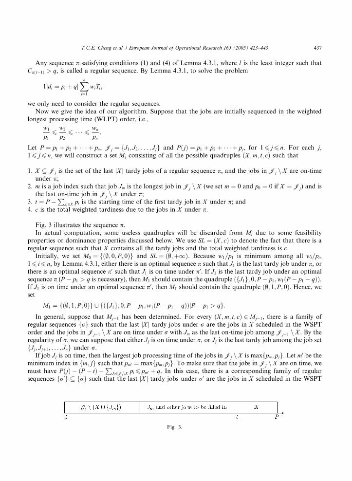
Let P ¼ p1 þ p2 þ � � � þ pn, Jj ¼ fJ1; J2; . . . ; Jjg and P ðjÞ ¼ p1 þ p2 þ � � � þ pj, for 16 j6 n. For each j,16 j6 n, we will construct a set Mj consisting of all the possible quadruples ðX ;m; t; cÞ such that

1. X � Jj is the set of the last jX j tardy jobs of a regular sequence p, and the jobs in Jj n X are on-time

under p;2. m is a job index such that job Jm is the longest job in Jj n X (we set m ¼ 0 and p0 ¼ 0 if X ¼ Jj) and is

the last on-time job in Jj n X under p;3. t ¼ P �

PJi2X pi is the starting time of the first tardy job in X under p; and

4. c is the total weighted tardiness due to the jobs in X under p.

Fig. 3 illustrates the sequence p.In actual computation, some useless quadruples will be discarded from Mi due to some feasibility

properties or dominance properties discussed below. We use SL ¼ ðX ; cÞ to denote the fact that there is a

regular sequence such that X contains all the tardy jobs and the total weighted tardiness is c.Initially, we set M0 ¼ fð;; 0; P ; 0Þg and SL ¼ ð;;þ1Þ. Because w1=p1 is minimum among all wi=pi,

16 i6 n, by Lemma 4.3.1, either there is an optimal sequence p such that J1 is the last tardy job under p, orthere is an optimal sequence p0 such that J1 is on time under p0. If J1 is the last tardy job under an optimal

sequence p (P � p1 > q is necessary), thenM1 should contain the quadruple ðfJ1g; 0; P � p1;w1ðP � p1 � qÞÞ.If J1 is on time under an optimal sequence p0, then M1 should contain the quadruple ð;; 1; P ; 0Þ. Hence, weset

M1 ¼ fð;; 1; P ; 0Þg [ fðfJ1g; 0; P � p1;w1ðP � p1 � qÞÞjP � p1 > qg:
In general, suppose that Mj�1 has been determined. For every ðX ;m; t; cÞ 2 Mj�1, there is a family of
regular sequences frg such that the last jX j tardy jobs under r are the jobs in X scheduled in the WSPT

order and the jobs in Jj�1 n X are on time under r with Jm as the last on-time job among Jj�1 n X . By the

regularity of r, we can suppose that either Jj is on time under r, or Jj is the last tardy job among the job set

fJj; Jjþ1; . . . ; Jng under r.If job Jj is on time, then the largest job processing time of the jobs in Jj n X is maxfpm; pjg. Let m0 be the

minimum index in fm; jg such that pm0 ¼ maxfpm; pjg. To make sure that the jobs in Jj n X are on time, we

must have P ðjÞ � ðP � tÞ �P

Ji2JjnX pi 6 pm0 þ q. In this case, there is a corresponding family of regular

sequences fr0g � frg such that the last jX j tardy jobs under r0 are the jobs in X scheduled in the WSPT

Fig. 3.

Fig. 4.

Fig. 5.


order, the jobs in Jj n X are on time under r0 with job Jm0 being the last on-time job among Jj n X , thestarting time of the jobs in X under r0 is t, and the total weighted tardiness of the jobs in X under r0 is c. Fig.4 illustrates the resulting sequence in this case.

If job Jj is tardy, then we must have P �P

Jj2X[fJjg pi > q, i.e., t � pj > q. In this case, there is a

corresponding family of regular sequences fr00g � frg such that the last jX j þ 1 tardy jobs under r00 are the

jobs in X [ fJjg scheduled in the WSPT order with Jj be the first tardy job among the job set X [ fJjg, thejobs inJj n ðX [ fJjgÞ ¼ Jj�1 n X are on time under r00 with Jm being the last on-time job among the jobs in

Jj�1 n X , the starting time of the jobs in X [ fJjg under r00 is t � pj, and the total weighted tardiness of the

jobs in X [ fJjg under r00 is cþ wjðt � pj � qÞ. Fig. 5 illustrates the resulting sequence in this case.Hence, we set

Mj ¼ fðX ;m0; t; cÞjðX ;m; t; cÞ 2 Mj�1; P ðjÞ � P þ t6 pm0 þ qg[ fðX [ fJjg;m; t � pj; cþ wjðt � pj � qÞÞjðX ;m; t; cÞ 2 Mj�1; t � pj > qg:

To reduce the computational effort, if there are two distinct elements ðX1;m1; t1; c1Þ and ðX2;m2; t2; c2Þ inMj such that m1 ¼ m2 ¼ m, t1 6 t2 and c1 6 c2, then the element ðX2;m2; t2; c2Þ should be removed fromconsideration. The proof is given in the Appendix A.

Furthermore, if ðX ;m; t; cÞ is an element in the Mj such that t � pm 6 q and c is as small as possible, then

there is a regular sequence p with the tardy job set X and total weighted tardiness c. The proof is given in

the Appendix A. Hence, if c < b (where b is the second component of SL), we revise SL by setting

SL :¼ ðX ; cÞ and delete any element ðX 0;m0; t0; c0Þ with c0 P c from Mj.

The above discussion leads to the following algorithm.

Algorithm 4.3.2. For 1jdi ¼ pi þ qjPn

i¼1 wiTi.Input: n jobs J1; J2; . . . ; Jn with processing times p1; p2; . . . ; pn, weights w1;w2; . . . ;wn, and SLK due-dates

di ¼ pi þ q, for 16 i6 n, respectively. Without loss of generality, we can suppose that the jobs are labelled

according to the WLPT order, i.e.,

w1

p16

w2

p26 � � � 6 wn

pn;

for otherwise, we can relabel the jobs in Oðn log nÞ time to obtain a required sequence.

Step 1. Compute

P ¼ p1 þ p2 þ � � � þ pn and

P ðiÞ ¼ p1 þ p2 þ � � � þ pi for 16 i6 n.Step 2. Set

M0 ¼ fð;; 0; P ; 0Þg,


SL ¼ ð;;þ1Þ andp0 ¼ 0.

Step 3. For j ¼ 1; 2; . . . ; n, do sub-steps (a)–(d).

M

(a) Let Mj ¼ ;.(b) For each element ðX ;m; t; cÞ of Mj�1, add to Mj the element ðX ;m0; t; cÞ if PðjÞ � P þ t6 qþ pm0 ,

where m0 is the minimum index in fm; jg such that pm0 ¼ maxfpm; pjg, and also add to Mj the

element ðX [ fJjg;m; t � pj; cþ wjðt � pj � qÞÞ if t � pj � q > 0 and cþ wjðt � pj � qÞ < b(where b is the second component of SL).

(c) Examine Mj for pairs of elements ðX ;m; t; cÞ and ðX 0;m; t; c0Þ with the same second component

and third component. For each such pair, delete ðX ;m; t; cÞ if cP c0, and delete ðX 0;m; t; c0Þotherwise.

(d) Let the element ðX ;m; t; cÞ (if any) in Mj be such that t � pm 6 q and c is as small as possible. If

c < b (where b is the second component of SL), revise SL by setting SL :¼ ðX ; cÞ and delete any

element ðX 0;m0; t0; c0Þ with c0 P c from Mj.

Step 4. Obtain the terminal SL ¼ ðX ; cÞ.

Output: An optimal sequence p with the tardy job set X being scheduled by the WSPT rule, and with the

other on-time jobs being scheduled by the SPT rule.

The following is a numerical example of the above algorithm. n ¼ 5, q ¼ 10, pj, wj and PðjÞ, 16 j6 n, areas follows.

For simplicity, we only compute each Mj and SL.

j 1 2 3 4 5

wj 1 3 4 5 4

pi 4 5 6 6 4

P ðjÞ 4 9 15 21 25

M0 ¼ fð;; 0; 25; 0Þg;

SL ¼ ð;;þ1Þ;

M1 ¼ fð;; 1; 25; 0Þ; ðfJ1g; 0; 21; 11Þg; and

M2 ¼ fð;; 2; 25; 0Þ; ðfJ2g; 1; 20; 30Þ; ðfJ1g; 2; 21; 11Þ; ðfJ1; J2g; 0; 16; 29Þg:

Since M2 has four elements, there will be eight possible elements for M3. But, for the tardy job set

X ¼ fJ1; J2; J3g, the starting time of the jobs in X is 10 ¼ q. Therefore, this X is eliminated in Step 3(b). So,

after Step 3(b),

M3 ¼ fð;; 3; 25; 0Þ; ðfJ3g; 2; 19; 36Þ; ðfJ2g; 3; 20; 30Þ; ðfJ2; J3g; 1; 14; 46Þ; ðfJ1g; 3; 21; 11Þ;ðfJ1; J3g; 2; 15; 31Þ; ðfJ1; J2g; 3; 16; 29Þg:

No element can be eliminated in Step 3(c). By noting that the element ðfJ1; J2g; 3; 16; 29Þ satisfies the criteriaof Step 3(d), we update SL and delete any element ðX 0;m0; t0; c0Þ with c0 P 29 from M3, includingðfJ1; J2g; 3; 16; 29Þ itself. Thus, after Step 3(d), we have

3 ¼ fð;; 3; 25; 0Þ; ðfJ1g; 3; 21; 11Þg and SL ¼ ðfJ1; J2g; 29Þ:


Similarly, M4 ¼ ; and M5 ¼ ;. Hence, the optimal sequence is

p ¼ ðJ5; J3; J4; J2; J1Þ;

and the objective value of p is 29.

Theorem 4.3.3. Algorithm 4.3.2 solves the problem


wiTi

in Oðn2PÞ time, where P ¼P

pi.

Proof. The correctness is implied in the preceding discussion leading to Algorithm 4.3.2. For the time

bound, notice that the size of each set Mj is no greater than nP , because there is at most one element in Mj

with the same second component and third component. Each update operation of Step 3(b) can be done in

OðnÞ time and be repeated for all OðnP Þ elements of Mj�1. Steps 3(c) and 3(d) require also Oðn2PÞ time,

because they can be implemented concurrently with Step 3(b). Hence, the theorem follows. h

For convenience in further discussion, we consider the following modified algorithm.

Algorithm 4.3.4. Modified algorithm for 1 di ¼ pi þ qj jPn

i¼1 wiTi:Let U be an upper bound of the optimal objective value. This algorithm is obtained from Algorithm

4.3.2 by initially setting SL ¼ ð;;UÞ and replacing Step 3(c) with the following Step 3(c0).

Step 3(c0) Examine Mj for pairs of elements ðX ;m; t; cÞ and ðX 0;m; t0; c0Þ with the same second component

and fourth component. For each such pair, delete ðX ;m; t; cÞ if tP t0, and delete ðX 0;m; t0; cÞotherwise.

Similar to Theorem 4.3.3, we have the following time bound for Algorithm 4.3.4.

Theorem 4.3.5. Algorithm 4.3.4 solves the problem

1 dij ¼ pi þ qXni¼1

wiTi

��
in Oðn2UÞ time, where Uð6
P16 j6 i6 n wipjÞ is an upper bound of the optimal objective value.

Remarks. The value of U in Theorem 4.3.5 can be chosen as U ¼ f ðp�Þ, where p� is the sequence obtained

by Modified Lawler’s Algorithm in Section 2, and so U is at most n� 1 times of the optimum.Suppose U > 0 in the sequel. Based on the fact that U is at most n� 1 times of the optimal objective

value, the following algorithm gives an FPTAS for the considered problem.

Algorithm 4.3.6. An FPTAS for 1jdi ¼ pi þ qjPn

i¼1 wiTi.Input: An arbitrary positive number e; n jobs J1; J2; . . . ; Jn with processing times p1; p2; . . . ; pn, weights

w1;w2; . . . ;wn and SLK due-dates di ¼ pi þ q, for 16 i6 n, respectively, such that

w1

p16

w2

p26 � � � 6 wn

pn:

Let U be the objective value of the sequence p� which is obtained by Modified Lawler’s Algorithm in

Section 2.


Step 1. Compute

K ¼ deUn2 e,P ¼ p1 þ p2 þ � � � þ pn and

P ðiÞ ¼ p1 þ p2 þ � � � þ pi, for 16 i6 n.Step 2. Set

M0 ¼ fð;; 0; P ; 0Þg,SL ¼ ð;;UÞ andp0 ¼ 0.

Step 3. For j ¼ 1; 2; . . . ; n do sub-steps (a)–(d).

(a) Let Mj ¼ ;.(b) For each element ðX ;m; t; cÞ of Mj�1, add to Mj the element ðX ;m0; t; cÞ if P ðjÞ � P þ t6 qþ pm,

where m0 is the minimum index in fm; jg such that pm0 ¼ maxfpm; pjg, and also add to Mj the

element ðX [ fJjg;m; t � pj; cþ Kbwjðt � pj � qÞ=KcÞ if t � pj � q > 0 and cþ Kbwjðt � pj �qÞ=Kc < b (where b is the second component of SL).

(c) Examine Mj for pairs of elements ðX ;m; t; cÞ and ðX 0;m; t0; cÞ with the same second component

and fourth component. For each such pair, delete ðX ;m; t; cÞ if tP t0, and delete ðX 0;m; t0; cÞotherwise.

(d) Let the element ðX ; ;m; t; cÞ (if any) in Mj be such that t � pm 6 q and such that c is as small as

possible. If c < b (where b is the second component of SL), revise SL by setting SL :¼ ðX ; cÞ anddelete any element ðX 0;m0; t0; c0Þ with c0 P c from Mj.

Step 4. Obtain the terminal SL ¼ ðX ;�cÞ.

Output: An ð1þ eÞ-approximation solution r with the tardy job set X being scheduled by the WSPT rule,

and with the other on-time jobs being scheduled by the SPT rule.

The important difference between Algorithms 4.3.6 and 4.3.2 arises in Step 3(b), which guarantees that

each Mj has at most OðnU=KÞ elements in Algorithm 4.3.6. The reader may find that the tardiness penalty

of each job Ji; is calculated by KbwiTi=Kc. The following result establishes that Algorithm 4.3.6 forms an

FPTAS.

Theorem 4.3.7. For any e > 0, Algorithm 4:3:6 is a ð1þ eÞ-approximation algorithm for the problem1jdi ¼ pi þ qj

Pni¼1 wiTi with a time requirement of Oðn4 1

eÞ.

Proof. Because each Mj has at most OðnUK Þ elements in Algorithm 4.3.6, the time requirement is at most

Oðn2 UKÞ ¼ Oðn4 1

eÞ. Let c be the optimal objective value of the considered problem. Let ðX ;�cÞ be the terminal

SL of Algorithm 4.3.6 and r be the corresponding sequence. For the reason that c is the optimal objective

value of the problem

1 dij ¼ pi þ q; p is regularXni¼1

KbwiTiðpÞ=Kc�� ;

and c is the optimal objective function value of the problem

1 dij ¼ pi þ q; p is regularXni¼1

wiTiðpÞ�� ;

we have cP�c. Furthermore, let c� be the total weighted tardiness under sequence r. By the optimality of c,we have c� P c and U 6 ðn� 1Þc < nc. We write c� ¼ f ðrÞ ¼

Pni¼1 wiTi. Then, �c ¼

Pni¼1 KbwiTi=Kc. Because


wiTi � KbwiTi=Kc6K � 16 eU=n2 6 �c=n, we have c� � c6 c� � �c ¼Pn

i¼1 ðwiTi � KbwiTi=KcÞ6 �c. This

implies c� 6 ð1þ eÞc and completes the proof. h

5. Concluding remarks

We present in this paper an Oðn2Þ time approximation algorithm for the general total weighted tar-

diness problem in a single machine. This algorithm can be treated as a more efficient alternative to theexisting dynamic programming and branch-and-bound algorithms for the problem. Due to the fact that

the general total weighted tardiness problem is NP-hard in the strong sense, many researchers have

turned to investigations of special models of the problems. We follow the same trend and analyze dif-

ferent special models of the problem, obtaining some interesting properties and results. We begin with the

model where the job due dates are affine-linear functions of their processing times and the tardiness

weights are proportional to their processing times. For this model, we successfully classify the NP-

hardness of the problem with respect to different affine-linear functions, and provide an Oðn log nÞalgorithm for each of the polynomially solvable problems. We continue to analyze the SLK due datemodel, and obtain the following results: the problem is NP-hard in the ordinary sense; a pseudo-poly-

nomial algorithm with time complexity Oðn2P Þ is derived; and a fully polynomial-time approximation

scheme is obtained.

The results in this paper have filled some gaps in the literature. These results may be helpful in devel-

oping new solution techniques and methods to tackle other aspects of the problems in the future. The

techniques used in this paper are theoretically challenging and may be applied to other earliness/tardiness

scheduling problems.

Acknowledgements

This research was supported in part by The Hong Kong Polytechnic University for Area of Strategic

Development under grant number A628. The third author was also supported by the National Natural

Science Foundation of China under grant number 10371112. The authors would like to thank two

anonymous referees for their helpful comments and recommendations. The present version of the paper has

benefited greatly from these comments.

Appendix A

The proofs of two statements are given in this Appendix A.

A.1. If there are two distinct elements ðX1;m1; t1; c1Þ and ðX2;m2; t2; c2Þ in Mj such that m1 ¼ m2 ¼ m, t1 6 t2and c1 6 c2, then the element ðX2;m2; t2; c2Þ should be left out of consideration.

Proof. Let frkg be the family of regular sequences corresponding to ðXk;mk; tk; ckÞ 2 Mj, k ¼ 1, 2. Let p2 be

an arbitrary sequence in fr2g. For every job J 2 fJmg [ fJjþ1; Jjþ2; . . . ; Jng, set sðJ ; p2Þ be the starting time

of J under p2. Since the jobs in fJmg [ fJjþ1; Jjþ2; . . . ; Jng should be scheduled from time PðjÞ � P þ tk � pmto time tk under rk, k ¼ 1, 2, there must be a sequence p1 2 fr1g such that the starting time of each job

J 2 fJmg [ fJjþ1; Jjþ2; . . . ; Jng is sðJ ; p2Þ � ðt2 � t1Þ6 sðJ ; p2Þ, and so the tardiness of job J under p1 is less

than or equal to the tardiness of job J under p2. Because c1 6 c2, the total weighted tardiness under p1 is

less than or equal to the total weighted tardiness under p2. Hence, ðX2;m2; t2; c2Þ should be deleted fromMj. h


A.2. If (X ;m; t; c) is an element in Mj such that t � pm 6 q and c is as small as possible, then there is a regular

sequence p with tardy job set X and total weighted tardiness c.

Proof. Let r be a regular sequence corresponding to ðX ;m; t; cÞ. Keeping the jobs in X unchanged in r,move job Jm to the position just before the jobs in X . Since t � pm 6 q, all the jobs in Jn n X are early no

matter how the jobs in Jn n ðX [ JmÞ are sequenced. Hence, there exists a regular sequence p with the tardy

job set X and total weighted tardiness c. h

References

[1] T.S. Abdul-Razaq, C.N. Potts, L.N. Van Wassenhove, A survey of algorithms for the single machine total weighted tardiness

scheduling problem, Discrete Applied Mathematics 26 (1990) 235–253.

[2] E.M. Arkin, R.O. Roundy, Weighted-tardiness scheduling on parallel machines with proportional weights, Operations Research

39 (1991) 64–81.

[3] K.R. Baker, Introduction to Sequencing and Scheduling, Wiley, New York, NY, 1974.

[4] T.C.E. Cheng, Optimal slack due-date determination and sequencing, Engineering Costs and Production Economics 10 (1986)

305–309.

[5] T.C.E. Cheng, M.C. Gupta, Survey of scheduling research involving due-date determination decisions, European Journal of

Operational Research 38 (1989) 156–166.

[6] T.C.E. Cheng, C. Oguz, X. Qi, Due date assignment and single machine scheduling with compressible processing times,

International Journal of Production Economics 43 (1996) 107–113.

[7] T.C.E. Cheng, M.Y. Kovalyov, Complexity of parallel machine scheduling with processing-plus-wait due dates to minimize

maximum absolute lateness, European Journal of Operational Research 114 (1999) 403–410.

[8] J.Z. Du, J.Y.-T. Leung, Minimizing total tardiness on one machine is NP-hard, Mathematics of Operations Research 15 (1990)

483–495.

[9] M.R. Garey, D.S. Johnson, Computers and Intractability: A Guide to the Theory of NP-Completeness, Freeman, San Francisco,

CA, 1979.

[10] D.S. Hochbaum, Approximation Algorithms for NP-Hard Problems, PWS, Boston, MA, 1997.

[11] J.E. Holsenback, R.M. Russell, R.E. Markland, P.R. Philipoom, An improved heuristic for the single-machine weighted-tardiness

problem, Omega, International Journal of Management Science 27 (1999) 485–499.

[12] H.G. Kahlbacher, T.C.E. Cheng, Processing-plus-wait due dates in single-machine scheduling, Journal of Optimization Theory

and Applications 85 (1995) 163–186.

[13] E.L. Lawler, Optimal sequencing of a single machine subject to precedence constraints, Management Science 19 (1973) 544–546.

[14] E.L. Lawler, A pseudopolynomial algorithm for sequencing jobs to minimize total tardiness, Annals of Discrete Mathematics 1

(1977) 331–342.

[15] E.L. Lawler, J.M. Moore, A functional equation and its application to resource allocation and sequencing problems, Management

Science 16 (1969) 77–84.

[16] J.K. Lenstra, A.H.G. Rinnooy Kan, P. Brucker, Complexity of machine scheduling problems, Annals of Discrete Mathematics 1

(1977) 343–362.

[17] C. Oguz, C. Dincer, Single machine earliness–tardiness scheduling problems using the equal-slack rule, Journal of the Operational

Research Society 5 (1994) 589–594.

[18] C.H. Papadimitriou, K. Steiglitz, Combinatorial Optimization, Prentice Hall, Englewood Cliffs, NJ, 1982.

[19] C. Potts, L. Van Wassenhove, A branch and bound algorithm for the total weighted tardiness problem, Operations Research 33

(1985) 363–377.

[20] L. Schrage, K.R. Baker, Dynamic programming solution of sequencing problems with precedence constraints, Operations

Research 26 (1978) 444–449.

[21] M.L. Smith, A. Seidmann, Due-date selection procedures for job-shop simulation, Computers and Industrial Engineering 7 (1983)

199–207.

[22] A. Volgenant, E. Teerhuis, Improved heuristics for the n-job single machine weighted tardiness problem, Computers and

Operations Research 26 (1999) 35–44.

[23] J.J. Yuan, The NP-hardness of the single machine common due date weighted tardiness problem, Systems Science and

Mathematical Sciences 5 (4) (1992) 328–333.

Single machine scheduling to minimize total weighted tardiness

Documents

Transcript of Single machine scheduling to minimize total weighted tardiness