Measuring the Impact of Living Wage Laws: A Critical Appraisal of David Neumark's How Living Wage...

POLITIC

AL EC

ON

OM

YR

ESEAR

CH

INSTITU

TE

10th floor Thompson HallUniversity of MassachusettsAmherst, MA, 01003-7510Telephone: (413) 545-6355Facsimile: (413) 545-2921 Email:[email protected]

Website: http://www.umass.edu/peri/

Measuring the Impact of Living Wage Laws:A Critical Appraisal of David Neumark's

How Living Wage Laws Affect Low-Wage

Workers and Low-Income Families

Mark D. Brenner

Jeannette Wicks-Lim

Robert Pollin

2002

Number 43

POLITICAL ECONOMY RESEARCH INSTITUTE

University of Massachusetts Amherst

WORKINGPAPER SERIES

PRELIMINARY DRAFT

MEASURING THE IMPACT OF LIVING WAGE LAWS:

A Critical Appraisal of David Neumark’s How Living Wage Laws Affect Low Wage Workers and Low-Income Families

Mark D. Brenner

Political Economy Research Institute University of Massachusetts-Amherst

[email protected]

Jeannette Wicks-Lim Department of Economics

University of Massachusetts-Amherst [email protected]

Robert Pollin

Department of Economics and Political Economy Research Institute University of Massachusetts-Amherst

[email protected]

October, 2002

ABSTRACT: Drawing on data from the Current Population Survey (CPS), David Neumark (2002) finds that living wage laws have brought substantial wage increases for a high proportion of workers in cities that have passed these laws. He also finds that living wage laws significantly reduce employment opportunities for low-wage workers. We argue, first, that by truncating his sample to concentrate his analysis on low-wage workers, Neumark’s analysis is vulnerable to sample selection bias, and that his results are not robust to alternative specifications that utilize quantile regression to avoid such selection bias. In addition, we argue that Neumark has erroneously utilized the CPS data set to derive these results. We show that, with respect to both wage and employment effects, Neumark’s results are not robust to more accurate alternative classifications as to which workers are covered by living wage laws. We also show that the wage effects that Neumark observes for all U.S. cities with living wage laws can be more accurately explained as resulting from effects on sub-minimum wage workers in Los Angeles alone of a falling unemployment rate and rising minimum wage in that city. ACKNOWLEDGEMENTS: We wish to thank David Neumark for providing us with the original data base and program files for his 2002 study. We are grateful to Jared Bernstein of the Economic Policy Institute, David Fairris of UC-Riverside, Peter Hall of UC-Berkeley, and Larry Katz of Harvard University for their detailed, perceptive comments on a previous draft. We especially acknowledge our University of Massachusetts colleague Michael Ash for his commitment and ongoing insights, which have been a major assistance throughout this project.

mailto:[email protected]



Measuring the Impact of Living Wage Laws: A Critical Appraisal of David Neumark’s

How Living Wage Laws Affect Low-Wage Workers and Low-Income Communities

Mark D. Brenner, Jeannette Wicks-Lim and Robert Pollin Department of Economics and Political Economy Research Institute

University of Massachusetts-Amherst

October, 2002

Non-Technical Summary of Working Paper

Since 1994 over eighty municipal governments in the United States have adopted so-called “living wage” ordinances. Most of the existing research has recognized the benefits of these laws for those workers who receive living wage increases and for their families But this research has also been clear in acknowledging the limitations of these measures in terms of affecting large numbers of the working poor.

David Neumark’s recent study finds that the effects of living wage laws are much broader

than this previous research has suggested. Building upon data provided in the monthly Current Population Survey (CPS), Neumark concludes that wages for as much as 11% of the low wage workforce may rise as a result of these measures in cities that adopt them, an estimate that is orders of magnitude beyond previous findings. Neumark also concludes that living wage laws reduce employment for the lowest wage workers in such cities by a significant degree. In short, Neumark finds that living wage laws pose a clear trade-off between higher wages versus fewer jobs.

This paper assesses the robustness of the Neumark’s findings, focusing primarily, as he

himself does, on the effects on wages. We also consider his findings with respect to employment. We find that Neumark’s findings are neither methodologically sound nor robust either statistically or substantively. To begin with, Neumark’s analysis relies on a statistical technique that is well-known to produce unreliable results. We briefly discuss the professional literature on this subject, then show that Neumark’s results are invalidated when we use an alternative statistical technique that controls for the problems faced by Neumark’s methodology.

We then proceed by accepting Neumark’s statistical approach on its own terms, and

within that context, raise other concerns with his analysis. Most broadly, we argue that the CPS cannot be effectively utilized in the manner deployed by Neumark, to detect the effects of living wage laws. In attempting to work with the CPS for this purpose, Neumark broadly classifies workers as among those “potentially covered” by living wage ordinances—i.e. those receiving legally mandated raises because of the implementation of living wage laws—without providing evidence as to whether his system of assigning “potential coverage” is consistent with the actual experiences of cities in implementing their ordinances. His decisions in selecting which workers should be included among those “potentially covered” to receive mandated raises several serious questions.

For example, Neumark includes workers who receive wages below the national or

relevant state-wide minimum wage—sub-minimum wage workers—as among those who have “potentially” received mandated living wage increases even though these workers are being paid

i

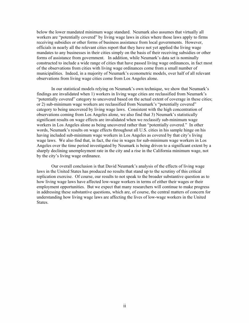
below the lower mandated minimum wage standard. Neumark also assumes that virtually all workers are “potentially covered” by living wage laws in cities where those laws apply to firms receiving subsidies or other forms of business assistance from local governments. However, officials in nearly all the relevant cities report that they have not yet applied the living wage mandates to any businesses in their cities simply on the basis of their receiving subsidies or other forms of assistance from government. In addition, while Neumark’s data set is nominally constructed to include a wide range of cities that have passed living wage ordinances, in fact most of the observations from cities with living wage ordinances come from a small number of municipalities. Indeed, in a majority of Neumark’s econometric models, over half of all relevant observations from living wage cities come from Los Angeles alone.

In our statistical models relying on Neumark’s own technique, we show that Neumark’s

findings are invalidated when 1) workers in living wage cities are reclassified from Neumark’s “potentially covered” category to uncovered based on the actual extent of coverage in these cities; or 2) sub-minimum wage workers are reclassified from Neumark’s “potentially covered” category to being uncovered by living wage laws. Consistent with the high concentration of observations coming from Los Angeles alone, we also find that 3) Neumark’s statistically significant results on wage effects are invalidated when we reclassify sub-minimum wage workers in Los Angeles alone as being uncovered rather than “potentially covered.” In other words, Neumark’s results on wage effects throughout all U.S. cities in his sample hinge on his having included sub-minimum wage workers in Los Angeles as covered by that city’s living wage laws. We also find that, in fact, the rise in wages for sub-minimum wage workers in Los Angeles over the time period investigated by Neumark is being driven to a significant extent by a sharply declining unemployment rate in the city and a rise in the California minimum wage, not by the city’s living wage ordinance.

Our overall conclusion is that David Neumark’s analysis of the effects of living wage

laws in the United States has produced no results that stand up to the scrutiny of this critical replication exercise. Of course, our results to not speak to the broader substantive question as to how living wage laws have affected low-wage workers in terms of either their wages or their employment opportunities. But we expect that many researchers will continue to make progress in addressing these substantive questions, which are, of course, the central matters of concern for understanding how living wage laws are affecting the lives of low-wage workers in the United States.

ii

1. Introduction and Summary of Findings

Since 1994 over eighty municipal governments in the United States have adopted so-

called “living wage” ordinances. While the specifics of these various measures differ, their

common theme is that they require firms doing business with local governments to pay minimum

wage rates that are well above both the U.S. and state-level minimum wage levels. The aim of

these laws is to set a wage floor high enough so that a full-time worker can support a family of

three or four at a living standard above the official poverty line. Most of the laws apply to large-

scale city service contractors, although a limited number also apply to firms receiving financial

assistance, tax abatements or other subsidies.

Most of the existing research has recognized the benefits of these laws for those workers

who receive living wage increases and for their families (see for example Pollin and Luce 2000,

Pollin and Brenner 2000, and Reich, Hall and Hsu 1999). But this research has also been clear in

acknowledging the limitations of these measures in terms of affecting large numbers of the

working poor. Indeed, most studies of both proposed and enacted living wage ordinances find

that these measures affect a very small number of private sector firms in a given locale, and that

the benefits of higher wages are concentrated among a small fraction of the overall workforce

within any given municipality (e.g. Pollin and Luce, op cit.; Niedt et al. 1999; Nissen 1998).

Recent work by David Neumark (2002) finds that the effects of living wage laws are

much broader than this previous research has suggested. Building upon data provided in the

monthly Current Population Survey (CPS), Neumark concludes that wages for as much as 11% of

the low wage workforce may rise as a result of these measures in cities that adopt them, an

estimate that is orders of magnitude beyond previous findings. Neumark also concludes that

living wage laws reduce employment for the lowest wage workers in such cities, with an

estimated employment elasticity of -.14. In short, Neumark finds that living wage laws pose a

clear trade-off between higher wages versus fewer jobs. But because Neumark also finds that the

positive wage benefits for low-wage workers have been stronger than the costs in terms of job

1

losses, the overall effect of these ordinances according to Neumark has been to reduce poverty in

cities that have adopted them.

Because of the importance of these questions to an accurate understanding of the

dynamics of living wage ordinances, this paper will assess the robustness of the Neumark’s recent

findings, focusing primarily, as he himself does, on the effects on wages. We also consider his

findings with respect to employment. We do not examine his analysis of poverty impacts, since

the viability of this analysis will hinge entirely on the prior analysis of wage and employment

effects.

Our overall conclusion is that Neumark’s findings are neither methodologically sound nor

robust either statistically or substantively. To begin with, Neumark’s econometric model relies

on a truncated sample of workers that excludes higher-wage workers from the data pool. While

Neumark’s approach is correct in focusing its attention on low-wage workers, the particular

manner in which he does so, through truncating the full sample, is vulnerable to sample selection

bias. This diminishes the reliability of his results, since they are subject to both bias and

inconsistency. We show that Neumark’s results are not robust when one takes an alternative

approach to truncation, that is, utilizing quantile regression.

But we then also accept Neumark’s truncation approach on its own terms, and within that

context, raise other concerns with his analysis. Most broadly, we argue that the CPS cannot be

effectively utilized in the manner deployed by Neumark, to detect the effects of living wage laws.

In attempting to work with the CPS for this purpose, Neumark broadly classifies workers as

among those “potentially covered” by living wage ordinances—i.e. those receiving legally

mandated raises because of the implementation of living wage laws—without providing evidence

as to whether his system of assigning “potential coverage” is consistent with the actual

experiences of cities in implementing their ordinances. His decisions in selecting which workers

should be included among those “potentially covered” to receive mandated raises several serious

questions.

2

For example, Neumark includes workers who receive wages below the national or relevant

state-wide minimum wage—sub-minimum wage workers—as among those “potentially covered”

by living wage laws, despite the fact that these workers aren’t being paid at the lower minimum

wage standard. Neumark also assumes that virtually all workers are “potentially covered” by

living wage laws in cities where those laws apply to firms receiving subsidies or other forms of

business assistance from local governments. However, officials in nearly all the relevant cities

report that they have not yet applied the living wage mandates to any businesses in their cities

simply on the basis of their receiving subsidies or other forms of assistance from government. In

addition, while Neumark’s data set is nominally constructed to include a wide range of cities that

have passed living wage ordinances, in fact most of the observations from cities with living wage

ordinances come from a small number of municipalities. Indeed, in a majority of Neumark’s

econometric models, over half of all relevant observations from living wage cities come from Los

Angeles alone.

Even in the models in which we accept Neumark’s sample truncation technique on its

own terms, we still show that all of Neumark’s statistically significant findings are invalidated

when 1) workers in living wage cities are reclassified from Neumark’s “potentially covered”

category to uncovered based on the actual extent of coverage in these cities; or 2) sub-minimum

wage workers are reclassified from Neumark’s “potentially covered” category to being uncovered

by living wage laws. Consistent with the high concentration of observations coming from Los

Angeles alone, we also find that 3) Neumark’s statistically significant results on wage effects are

invalidated when we reclassify sub-minimum wage workers in Los Angeles alone as being

uncovered rather than “potentially covered.” In other words, Neumark’s results on wage effects

throughout all U.S. cities in his sample hinge on his having included sub-minimum wage workers

in Los Angeles as covered by that city’s living wage laws. We also find that, in fact, the rise in

wages for sub-minimum wage workers in Los Angeles over the time period investigated by

3

Neumark is being driven to a significant extent by a sharply declining unemployment rate in the

city and a rise in the California minimum wage, not by the city’s living wage ordinance.

The rest of the paper is structured as follows: In Section 2, we present an explanation and

replication of Neumark’s basic findings for wages and employment. In Section 3 we discuss

methodological shortcomings with the Neumark’s analysis. In Sections 4 and 5, we re-estimate

his findings for wage effects and employment effects of living wage laws on the basis of both and

alternative econometric methods and alternative choices as to which workers should be classified

as likely to have received mandated living wage increases. Section 6 concludes.

2. The Neumark Model – Explanation and Replication

In his 2002 Public Policy Institute of California (PPIC) Report “How Living Wage Laws

Affect Low Wage Workers and Low-Income Families,” Neumark uses data from the Current

Population Survey (CPS) to measure the effect of living wages on the wages and employment

status of low wage workers during the 1996-2000 period. Specifically, Neumark constructs a

pooled cross section of observations from the CPS, utilizing all persons in cities with at least 25

observations in a given month of the calendar year.1 Taking a difference-in-difference approach,

he then attempts to gauge living wage effects by analyzing low wage workers in large cities with

and without living wage laws over the period in question. We will first describe his methods for

assessing the effect of living wage laws on the earnings of low-wage workers and then turn to his

employment analysis. Our remarks will focus on the three models from which he derives his basic

findings.

1 In the wage analysis, the sample is constructed from observations of employed persons earning an hourly wage greater than $1.00 and less than or equal to $100. In both the wage and employment analysis, observations are restricted to individuals between the ages of 16 and 70, inclusive.

4

Wage Analysis

Equation 1 presents the first model that Neumark employs to assess the effect of living

wage laws on low-wage workers’ earnings:

(1) ln(wicmy) = α + Xicmyω + βln(wmincmy) + γmax[ln(wliv

cmy),ln(wmincmy)] +

δyYy + δMMm + δCCc + εicmy

Here Neumark estimates a wage equation where w is the hourly wage, X is a vector of dummy

variables controlling for gender, race, education, and marital status, wmin is the higher of the

federal and state minimum wage, and wliv is the higher of the prevailing minimum wage or

applicable municipal living wage (our notation throughout mirrors that in Neumark’s study). Y,

M, and C are vectors of dummy variables controlling for each year, month, and city respectively.

The unit of analysis (denoted by the subscript of icmy) is the individual worker, within a given

city c, month m, and year y. Note that β captures the effect of the minimum wage (state or

federal) on individual worker wages, and γ captures the wage effect of the living wage on

workers’ wages.

Neumark employs a second model that attempts to discriminate between the wage effect

of living wage ordinances experienced by “covered” workers versus those experienced by

“uncovered” workers. In classifying workers as covered or uncovered, Neumark distinguishes

between two types of living wage ordinances. The first type of law applies only to those firms

that perform services under contract with a municipality. These usually include such services as

landscape maintenance or security guard and janitorial services. For these “contractor-only”

ordinances, covered workers are defined to be those individuals working in service industries

(usually about 10-20% of the workforce).

The second type of living wage ordinance he identifies applies to any firm that receives a

designated form of financial assistance (such as utility subsidies, tax abatements, or industrial

revenue bond guarantees, etc.) from a municipality. For ordinances with such “business-

5

assistance” provisions, covered workers are defined to be all private sector workers (usually about

90-95% of the workforce), since any business in the private sector could potentially receive

financial assistance from its local government. It is important to emphasize that, unlike most

other researchers on this issue, Neumark makes no attempt to determine which firms and workers

are actually likely to be covered according to the stipulations of the living wage ordinances in any

given municipality. He rather relies on broad assumptions as to which workers are “potentially”

covered, then proceeds with his estimation exercises through including all “potentially” covered

workers in his data sample. As we will see, Neumark’s assumptions as to who should be

included in the pool of potentially covered workers are crucial to his overall findings.

Equation 2 presents the second model used by Neumark:


cmy) x Covicmy,ln(wmincmy)] +

γ’max[ln(wlivcmy) x Uncovicmy,ln(wmin

cmy)] + δyYy + δMMm + δCCc + εicmy

Here Cov is a dummy variable equal to one for covered workers and Uncov is a dummy variable

equal to one for workers who are not covered. Note that while β still controls for the wage effect

of the minimum wage, γ and γ’ capture the separate wage effects of the living wage for covered

and uncovered workers, respectively.2

In his third model, Neumark returns to the specification in equation 1, but also attempts

to distinguish between the effects of contractor-only versus business-assistance living wage laws.

Equation 3 depicts this approach:


cmy) x Busicmy,ln(wmincmy)] +

γ’max[ln(wlivcmy) x Conicmy,ln(wmin

cmy)] + δyYy + δMMm + δCCc + εicmy

Here Bus is a dummy variable equal to one for workers living in a city with a living wage

ordinance that includes a business assistance provision and Con is a dummy variable equal to one

for workers living in a city with a contractor-only living wage ordinance. Again, β controls for

6

the effect of the minimum wage on individual wage levels, and γ and γ’ capture the different

wage effects of business-assistance type living wage ordinances and contractor-only type living

wage ordinances respectively.

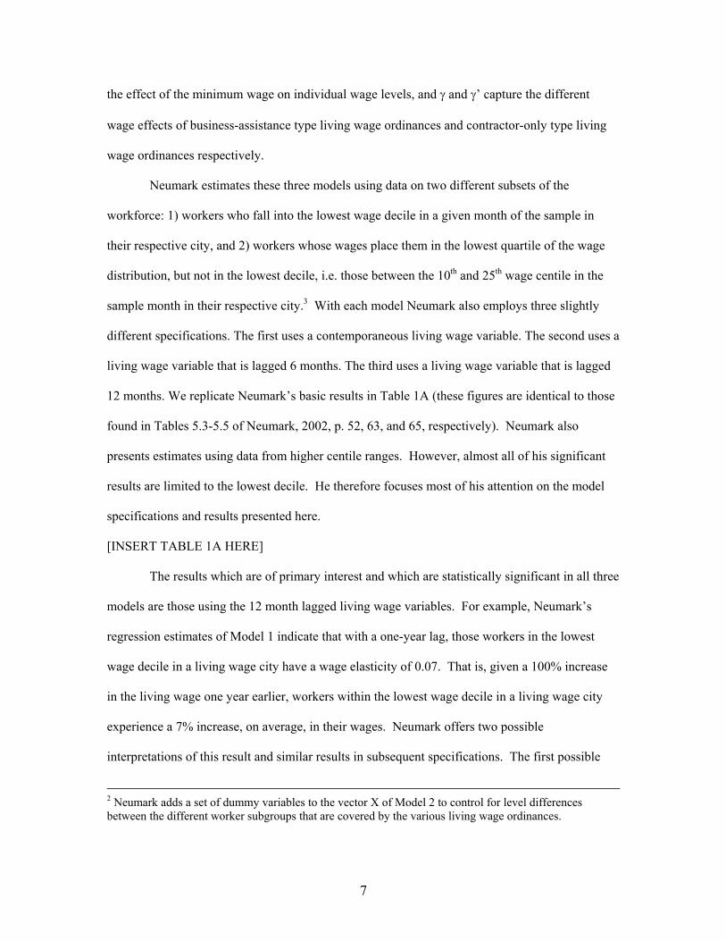
Neumark estimates these three models using data on two different subsets of the

workforce: 1) workers who fall into the lowest wage decile in a given month of the sample in

their respective city, and 2) workers whose wages place them in the lowest quartile of the wage

distribution, but not in the lowest decile, i.e. those between the 10th and 25th wage centile in the

sample month in their respective city.3 With each model Neumark also employs three slightly

different specifications. The first uses a contemporaneous living wage variable. The second uses a

living wage variable that is lagged 6 months. The third uses a living wage variable that is lagged

12 months. We replicate Neumark’s basic results in Table 1A (these figures are identical to those

found in Tables 5.3-5.5 of Neumark, 2002, p. 52, 63, and 65, respectively). Neumark also

presents estimates using data from higher centile ranges. However, almost all of his significant

results are limited to the lowest decile. He therefore focuses most of his attention on the model

specifications and results presented here.

[INSERT TABLE 1A HERE]

The results which are of primary interest and which are statistically significant in all three

models are those using the 12 month lagged living wage variables. For example, Neumark’s

regression estimates of Model 1 indicate that with a one-year lag, those workers in the lowest

wage decile in a living wage city have a wage elasticity of 0.07. That is, given a 100% increase

in the living wage one year earlier, workers within the lowest wage decile in a living wage city

experience a 7% increase, on average, in their wages. Neumark offers two possible

interpretations of this result and similar results in subsequent specifications. The first possible

2 Neumark adds a set of dummy variables to the vector X of Model 2 to control for level differences between the different worker subgroups that are covered by the various living wage ordinances.

7

interpretation Neumark offers is that, given that the maximum wage elasticity we would expect

for a covered worker would be 1, the .07 elasticity represents the proportion of workers in the

lowest decile that receive the full living wage raise—that is, seven percent of all workers in this

lowest decile are receiving the living wage increase. The second possible interpretation is that

workers earning the living wage increase now earn wages that place them in a higher wage decile.

This “bumping up” effect would then mean that the mean wage for the lowest decile would rise,

since the decile would now include workers whose wages had previously placed them in the next

higher decile. As Neumark notes, this second interpretation of his results can also incorporate

disemployment effects. That is, if some workers in the lowest decile become nonemployed due

to the living wage and therefore drop out of the pool of wage earners, that would mean that the

newly constituted lowest decile would now include workers earning higher wages. In our

analysis of Neumark’s findings, we find that his first explanation cannot be supported by the

relevant evidence, but that his second explanation is empirically possible. However, it is another

matter whether this second interpretation is consistent with the full range of relevant evidence.

In Model 2, with a one-year lag, those workers living in a living wage city and

categorized as “covered” have a wage elasticity of 0.11. Those who live in a city that has a living

wage ordinance that was enacted one year previously and are categorized as “uncovered” are

statistically indistinguishable from those workers who live in cities that did not have living wage

ordinances enacted in the prior year. Finally, in Model 3, with a one-year lag, those workers

living in a city that has a living wage ordinance that includes a business assistance provision have

a wage elasticity of 0.11. Those workers living in a city that had a living wage ordinance one

year prior that targets contractors only are indistinguishable statistically from those workers who

live in cities that did not have any type of living wage ordinance enacted one year before. Thus

Neumark concludes that only those workers in cities where living wage laws have business-

3 Neumark also presents estimates using data from higher centile ranges but because virtually all of his significant results are limited to the lowest decile, he focuses most of his attention on the two subsets

8

assistance clauses appear to have a statistically significant wage effect. Our regression estimates

yield identical results, namely wage elasticity estimates of 0.07, 0.11, 0.11 in Models 1, 2 and 3

respectively.

Note that Neumark also finds a statistically significant effect for the living wage variable

lagged six months for covered workers in Model 2 and for business assistance cities in Model 3.

In both cases the magnitude of the living wage coefficient is approximately half that of the

coefficient for the living wage variable lagged 12 months. Although Neumark does not highlight

the statistically significant results for the six month lagged specification, in all subsequent

analysis we examine this specification as well as the twelve month lag.

In Table 1B we include a model specification that is not presented in Neumark’s original

work, but which draws directly from it, that is:


cmy) x Busicmyx Covicmy,

ln(wmincmy)] + γ’max[ln(wliv

cmy) x ConicmyxCovicmy, ln(wmincmy)] + θmax[ln(wliv

cmy)

x Busicmyx Uncovicmy, ln(wmincmy)] + θ’max[ln(wliv

cmy) x ConicmyxUncovicmy,

ln(wmincmy)]+δyYy + δMMm + δCC

c + εicmy

What we call Model 4 combines the covered/uncovered distinction of Neumark’s Model 2, with

the contractor-only/business assistance distinction drawn in his Model 3. In this instance positive

and statistically significant coefficients on γ ( γ’) would indicate that covered workers in business

assistance (or contractor-only) cities were receiving wage increases as a result of the respective

living wage laws. By contrast if θ (θ’) displays a positive and statistically significant coefficient,

this instead means that uncovered workers in living wage cities are experiencing wage increases.

As can be seen from Table 1B, which presents results for the lowest decile and both the 6 and 12-

month lagged specification, results from our Model 4 appear to confirm Neumark’s findings that

it is covered workers in business assistance cities who are receiving wage increases as a result of

described in the text.

9

the passage of living wage laws. Specifically we estimate a wage elasticity of .11 for the 12

month lagged specification and .07 for the six month lagged specification.

[INSERT TABLE 1B HERE]

Employment Analysis

The framework Neumark employs for analyzing the effect of living wage laws on

employment mirrors his wage analysis discussed above. Specifically Neumark utilizes a linear

probability model to assess the effect that living laws have on the employment status of

individuals throughout the wage distribution. One significant difference between the wage and

employment models, however, is that the employment model incorporates individuals currently

outside the labor force into the analysis. As such, Neumark is required to impute wages for non-

working individuals, in order to place them within the overall wage distribution. For consistency,

Neumark then calculates imputed wages for all workers, including those holding jobs, and utilizes

these imputed wage rates, rather than actual wages for the employed workers, in establishing

decile thresholds.

We reproduce Neumark’s initial employment results in Table 2A (these figures are

identical to those found in Tables 6.1 and 6.2 of Neumark, 2002, p. 82-3). Consistent with

Neumark’s original results, for Model 1 we find a negative statistically significant effect of living

wage laws, lagged 12 months, on employment status for those individuals in the lowest wage

decile. The estimated coefficient is –5.62. Given that the average employment rate for the lowest

decile is approximately .4, this implies an elasticity of -.14 (i.e -.056/.4). In other words, these

results suggest that for a 100 percent increase in wages generated through the living wage

mandate, the employment rate for the lowest decile of workers would decline by 14 percent.

But note with Neumark’s Model 1 results the additional statistically significant findings.

That is, in four specifications with data from the 25th-50 and 50th-75th centile ranges, Neumark

finds that the living wage laws exert a statistically significant positive influence on the

employment rate. These results would appear anomalous—that the living wage laws would, first

10

exert any significant influence on employment for highly-paid workers; and second, that any such

employment effect due to rising wages would be positive rather than negative. Neumark provides

a one-sentence aside on these findings, offering the possibility that the living wage increase is

responsible for producing proportionally more high-end jobs. But he offers no evidence to

corroborate this hunch.

Considering now Neumark’s Model 3, we also find a statistically significant effect for the

living wage 12 months lagged within the lowest wage decile in business assistance cities, with an

estimated coefficient of –5.88, implying an elasticity of -.15.

[INSERT TABLE 2A HERE]

One advantage that arises when modeling employment status as opposed to wages is that

using working and nonworking individuals dramatically increases the number of cities for which

Neumark’s inclusion criteria of 25 observations in a given city-month cell are met. In all,

Neumark uses a total of 223 cities in his employment analysis, as compared with the 130 cities

that he is able to use in his wage analysis. A natural question that arises, however, when

juxtaposing results from the wage and employment analysis, is whether the statistical significance

of Neumark’s employment results would remain if the analysis were conducted on the same set of

cities used for his wage analysis. This question is especially germane in light of the fact that

Neumark himself notes that “[t]he evidence on employment effects is weaker than the evidence

on wage effects,” (ibid, p. 86). As seen in Table 2B, Neumark’s findings appear to hold for the

restricted set of cities. For Model 1 we find a statistically significant effect for the 12 month lag

of living wage laws in the lowest wage decile, with an estimated coefficient of –4.8. For Model 3

we also find a statistically significant effect in business assistance cities, with an estimated

coefficient of –5.34 for the living wage lagged 12 months. In both cases the coefficients (and

implied elasticities) are smaller than those estimated using the larger set of cities. The statistical

significance is also weaker in the Model 3 specification.

[TABLE 2B BELONGS HERE]

11

3. Assessing the Neumark Approach

In this section we discuss several potential limitations to Neumark’s methodological

approach and examine several potentially problematic features of the features of his data sample.

Sample Truncation and Selection Bias

Neumark’s focuses his analysis of living wage laws on workers at the lower portions of

the wage distribution. Indeed, as we have seen, he obtains statistically significant effects of living

wage laws only when he narrows his data set to include workers in the lowest decile of the overall

wage distribution. The methodology Neumark employs here is known as a truncation of the full

data set.

Given that the living wage laws are of course targeted at benefiting low-wage workers,

not all workers, it is appropriate that Neumark’s analysis be focused on the lowest-paid workers

only. However, as has been demonstrated in the literature, Neumark’s method of truncation is

vulnerable to selection bias, since he is truncating the full sample based on workers’ wages, the

dependent variable in the model. This approach to truncation can produce both biased and

inconsistent estimates of model coefficients (see Maddala 1983). The recent survey article by

Koenker and Hallock (2001) provides several practical illustrations where the type of truncation

employed by Neumark can create a seriously distorted statistical picture.4

As Koenker and Hallock make clear, a more appropriate econometric technique with

which one can focus attention on the lower wage distribution while avoiding the selection bias

associated with truncated regression is quantile regression. This is because with a quantile

regression, one can choose the central tendency point around which to estimate a regression—for

example, wages at the 10th decile rather than the mean—without truncating the sample to exclude

the upper 90 percent of workers from the analysis. Koenker and Hallock provide numerous

4 One of the examples Koenker and Hallock describe is Engel’s classic analysis of the relationship between food expenditure and household income. In this case, they show how a truncation on the dependent variable such as Neumark performed “would yield disastrous results.” They further comment that “such

12

examples in which the quantile regression technique has been used in recent years in labor

econometric models. In the next section of the paper, we perform a quantile regression on

Neumark’s data sample.

Sample Size Issues

Unlike analysis at the national level, utilizing the Current Population Survey to study

local area labor markets can frequently be difficult, due to relatively small sample sizes. This is

particularly true if the analysis is concentrated on a subset of the local-area labor market (in our

discussion we take the local area labor market to be the Metropolitan Statistical Area – MSA).

Although Neumark utilizes data from a broad range of cities, the analysis fundamentally is one of

local area labor markets, since it is within the MSA that the difference-in-difference methodology

applies.

This general problem of small sample sizes for local areas is exacerbated by the specific

task of detecting the effects of living wage laws in which, according to previous researchers, the

number of workers affected by the laws will be a very small proportion of the total low-wage

labor force. Take for example the case of Los Angeles. In 1999 there were approximately 4.6

million people in the Los Angeles labor market (i.e. the Los Angeles-Long Beach Primary MSA).

Pollin and Luce (2000) had estimated that, as of 1999, the LA living wage ordinance would cover

no more than 7,600 employees, that is, no more than 1 in 600 workers in the local LA labor

market. Given that in 1999 the CPS sampled approximately 5000 wage earners in the Los

Angeles-Long Beach PMSA, this implies that there are likely to be about eight workers covered

by the living law within this sample5. This number is too small a number to obtain statistically

reliable estimates.

strategies are doomed to failure for all the reasons so carefully laid out in Heckman’s (1979) work on sample selection.” 5 The estimate of eight covered workers in the CPS sample is derived as follows: 7,600 is 0.17 percent of the full 4.6 million workforce in Los Angeles. The CPS sample is approximately 5,000 workers, and 0.17 percent of 5,000 is approximately eight.

13

The crucial question to ask here therefore is: what is the probability that a large enough

number of workers receiving a living wage would be included in the CPS sample? Assume we

set 25 as the minimum number of workers receiving living wage increases necessary to conduct

meaningful statistical analysis. If it is in fact the case that about 7,600 workers are covered by the

law, then the odds that 25 or more will be included in the CPS sample of 5,000 are approximately

one in 500,000. If we assume 30 to be the minimum necessary number for the CPS sample, then

the odds of including that number or more in the CPS sample rise to one in 244 million.6

The problem is complicated further by the fact that even if directly affected workers were

in the sample, there is no way within the CPS data of identifying who they are. Such a

determination would require information about individuals’ primary employers, as well as

information from the city as to which private sector firms were covered by their living wage law.

Because of these data limitations, Neumark adopts the method described above for identifying

“potentially” covered workers. Thus, to take the Los Angeles example once again, under

Neumark’s definition, 97 percent of the Los Angeles low-wage labor market is “potentially”

covered by the LA living wage ordinance, which translates into approximately 450,000 workers

within the lowest wage decile in Los Angeles being in the “potentially covered” category.

Figures of this magnitude are far beyond what any previous observer had suggested was even a

most high-end estimate of the coverage range for living wage laws.

6 The exact formula for determining the probability of 25 or more workers covered by the LA living wage ordinance appearing in the Current Population Survey is:

∑≥

−−−25

)5000()1()!5000(!

!5000k

kk ppkk

In this calculation, 5000 is the approximate sample size drawn from the Los Angeles-Long Beach PMSA while k is the number of covered workers in the CPS and p is the probability that a given individual will be a covered worker. Based on the fact that there were approximately 4.6 million labor force participants in the Los Angeles-Long Beach PMSA in 1999, and approximately 7,600 covered workers at that time, p=7,600/4,600,000.

14

It is important to note, moreover, that Neumark is not referring with this category of

“potentially covered” workers to those who may be receiving non-mandated “ripple effect” wage

increases—i.e. those workers whose employers give them raises after a living wage law passes

even though the living wage law does not mandate that this be done. It is certainly true that living

wage laws, like minimum wage laws, do generate some ripple wage increases for noncovered

workers. But none of the existing literature on this topic suggests that such ripple effects are

orders of magnitude larger in terms of number of workers getting raises than the mandated wage

increases, nor does Neumark introduce any arguments or evidence to support such a position.7

Indeed, Neumark never claims that his category of “potentially covered” workers includes

workers receiving non-mandated ripple effect raises. He is clear, rather, that his category of

“potentially covered” workers includes all workers employed in industries where businesses

could potentially be mandated to provide living wage increases (see Neumark 2002, pp. 58 – 61).

Living Wage Effects on Sub-Minimum Wage Workers

Our next major concern is Neumark inclusion of sub-minimum wage workers in his data

pool without having provided a careful explanation as to why it is reasonable to do so. Sub-

minimum wage workers could possibly benefit through a ripple effect from a mandated living

wage increase. But because, by definition, they are not receiving mandated minimum wage

increases, it is difficult to see how they would qualify as among those “potentially covered” to

receive mandated living wage increases. Neumark’s decision to include sub-minimum wage

workers as among those potentially covered is especially important given that it is only in the

lowest decile of the wage distribution that Neumark finds statistically significant effects from

living wage laws. Yet, as Neumark reports in Table 1.4 of his study, the upper bound for the 10th

decile in many cities is frequently at or only slightly above the relevant minimum wage (Neumark

7 See Pollin and Brenner (2000), pp. 49–55 for one effort at utilizing the existing literature on minimum wage ripple effects to projecting its potential magnitude for the case of the living wage ordinance in Santa Monica, CA. Some of the more recent literature on minimum wage ripple effects includes Katz and Krueger (1992) and Card and Krueger (1995).

15

2002, p. 7). In fact, we estimate that over a quarter of workers in the lowest decile are earning

less than the relevant minimum wage over the entire sample period, and in many cities this

number is considerably higher. The highest proportion is for Los Angeles, in which a full 39

percent of Neumark’s data pool for the lowest decile are sub-minimum wage workers.8

The Definition of Coverage with Business-Assistance Clauses

Another concern with Neumark’s methodology is his approach for defining coverage in

cities where business-assistance recipients are covered by living wage laws. As discussed above

for Los Angeles, for all practical purposes Neumark is including the entire labor force as

potentially covered by the law. While Neumark acknowledges that this classification of business-

assistance coverage will be “noisy”, we would go further: this classification is not consistent with

the available evidence of how living wage laws have actually been implemented. We draw this

conclusion after conducting personal interviews with city officials in all the cities classified by

Neumark himself as having business assistance clauses in their living wage ordinances. Our goal

was to determine the extent to which these cities were in fact applying the business-assistance

clause in their living wage laws. Based on our interviews with city staff, we found that, with the

exception of San Antonio, none of the cities in Neumark’s study had actually implemented the

business assistance provision in their living wage law during the period 1995 to 1999.9

This has two important implications. First, for all cities currently classified as business-

assistance cities, the category of “potentially covered” workers should include, at most, only

workers in the likely-to-be-affected service industries (that is, 10-20% of the workforce in those

cities rather than 90-95%). Second, adjusting the “potentially covered” category to conform with

the evidence runs counter to Neumark’s claim that it is the “broadness” of the business-

assistance-type living wage ordinances that explains the detectable increase in wages due to

8 It is also important to note that over the entire sample period approximately 10 percent of the lowest decile is comprised of workers earning exactly the minimum wage. This implies that more than a third of the lowest decile is earning at or below the prevailing minimum wage.

16

living wage ordinances.10 Rather, the business-assistance-type living wage ordinances are not, in

practice, broader than the contractor-only living wage ordinances.11

The Geographic Distribution of Covered Workers

Another methodological issue is the geographic distribution of covered workers in the

lowest decile in both Neumark’s wage and employment analysis. Panel A of Table 3 presents the

number of affected workers in each living wage city for Models 1-3 with a 12 month lagged

specification. We focus only on the 12 month lagged specification for the sake of brevity. The

geographic distribution of covered workers in the 6 month lagged specification closely follows

that presented in Table 3.

[INSERT TABLE 3 HERE]

A crucial fact that emerges from this table is that most of the covered workers are located

in a very small number of cities. Indeed for Models 2 and 3 of the wage analysis, approximately

half of all affected workers are found in Los Angels alone. Panel B of Table 3 presents similar

estimates for Neumark’s employment analysis, and here too Los Angeles has a disproportionate

share of the total number of affected workers, including 54% of all affected workers in Model 3.

Neumark makes no mention of this geographic concentration of his data pool in his study.

The concentration of affected workers in Los Angeles and a handful of other cities is due

to three main factors. The first is the differential size of the cities themselves, with Los Angeles

having the largest population among the living wage cities in Neumark’s data pool. The second

is the nature of the ordinances in the different cities. Using Neumark’s classifications, cities with

business assistance clauses have a much larger pool of “potentially covered” workers than those

with “contractors only” ordinances. However the most important factor is the year in which

9 Telephone interviews with Apney (10/30/01), Enman (10/30/01), Gibson (10/18/01), Greyson (10/15/01), Jacobson (10/29/01), and Robbins (10/23/01). Full citations to interviews are in the reference section. 10 Neumark concludes his analysis of the effects on wages of living wage laws by writing, “the effects are driven by cities in which the coverage of living wage laws is more broad—namely, cities that impose living wages on employees receiving business assistance from the city,” (Neumark 2002, pp. 73-4).

17

living wage laws were adopted in each city. In the cases of Los Angeles and Minneapolis, both

adopted their living wage laws in 1997. This implies that in both cities workers are classified as

affected for nearly a year more than in every other living wage city. This also explains why cities

such as Hartford, where their living wage ordinance was not passed until October 1999, have so

few workers classified as affected in the 12 month lagged specification. As we shall see in the

next section, the geographic concentration of covered workers is central to explaining Neumark’s

statistically significant results.

Increasing wages and employment

As we have seen, Neumark finds that living wage laws produce a statistically significant

negative employment effect on workers within the lowest decile—that is, there is a lower

employment rate among low-wage workers after living wage laws are implemented than before.

Of course, Neumark did also find an anomalous statistically significant positive employment

effect for high-wage workers due to living wage laws. But focusing on the result for low-wage

workers only, Neumark interprets this negative employment effect as representing disemployment

among low-wage workers, i.e. that low-wage workers are involuntarily facing diminished

employment prospects. But Neumark is neglecting here the well-known literature on labor force

participation decisions resulting from wage increases, such as would occur through a living wage

ordinance. This issue is especially pertinent given that more than two-thirds of the workers in the

lowest decile of Neumark’s data pool are women, whose labor force participation decisions are

well known to be more complex than those for similarly-profiled men (see for example the

discussions in Killingsworth and Heckman 1986, Eissa and Liebman 1996, and Eissa and Hoynes

1998). For example, as Eissa and Hoynes have demonstrated with respect to the earned income

tax credit program, the increased earning opportunities afforded by the program do not

necessarily increase women’s labor force participation and are likely to reduce participation in

11 For example, even in San Antonio, the only city to implement their business assistance clause in the period, fewer than 10 businesses were covered by the law during the 1996-00 period.

18

the case of married women. For these women in the low-wage labor market, an increase in their

take-home pay has enabled them to voluntarily cut back on their hours of work. Their reduction

in employment is not due to an involuntary loss of employment. At least for some significant

subset of low-wage workers, especially women, one might anticipate some analogous effects to

operate in the case of living wage laws. Neumark does not explore this possibility.

4. Re-Examining Neumark’s Analysis of Wage Effects

In light of the above concerns, we now reexamine Neumark’s econometric results on the

wage effects of living wage ordinances.

Quantile Regression

In Table 4, we present results from testing Neumark’s models 1-3 using quantile

regression centered on the 10th wage decile. We report results only for the living wage variable

lagged 12 months, that is, the variable on which Neumark himself concentrates his attention. As

we see, making this one methodological adjustment on Neumark’s model to control for sample

selection bias produces substantially different results than Neumark obtained through his

truncated regression technique, whose results we reported in our Table 1A.

INSERT TABLE 4 HERE

With Model 1, covering all living wage laws, we now find that the coefficient value on

the living wage variable has fallen nearly 10-fold—from 6.95 in Neumark’s model to 0.74 and is

not statistically significant. With Model 2, in which the sample is divided according to

Neumark’s categories of “potentially covered” and uncovered workers, we do still obtain a

statistically significant coefficient for covered workers at the 10 percent level. However, the

coefficient on this variable has now fallen more than 3-fold, from 10.61 under Neumark’s

specification to 3.04 with the quantile regression. Finally, in our quantile regression of

Neumark’s Model 3, the coefficient for “business assistance” living wage cities again falls nearly

10-fold and is insignificant. In short, we see that Neumark’s results are not robust after

controlling for sample selection bias through quantile regression, but making no further

19

adjustments to his methodology. At the very least, these results raise questions as to the overall

robustness of Neumark’s findings, and, more generally, his methodology of relying exclusively

on truncated OLS regressions. Nevertheless, having raised these questions, we will now proceed

through accepting as is his truncated OLS methodology, and addressing our other concerns with

his methodology.

Correcting the Coverage Classification in Business-Assistance Cities

We now consider the issue of how Neumark chose to classify workers as among those

“potentially covered” to receive mandated wage increases due to living wage ordinances. As

discussed earlier, no living wage city but San Antonio has actually implemented their business-

assistance clause between 1995 and 1999, the relevant years for the 12 month lagged

specification.12 How would Neumark’s results be affected by classifying workers in business

assistance cities in a manner reflective of the actual experiences in these cities? To assess this,

we re-estimated Neumark’s Model 2 and our Model 4 classifying workers in business assistance

cities as “potentially covered” only if they worked in the service industry.13 Our revised wage

equation results for the lowest decile are presented in Table 5. We present results for both the 6

and 12 month lagged specification.


As is clear from the table, reclassifying potentially covered workers to more accurately

reflect how living ordinances are being implemented substantially alters Neumark’s original

findings. Indeed, based on our revised classification, we find that there is no measurable wage

effect of living wage ordinances on potentially covered workers for either the 6 or 12 month

specification. In fact, we observe a statistically significant, positive wage effect of living wages

for uncovered workers in the 12 month lagged specification for Model 2, and in both the 6 and 12

12 It also merits note that in the San Antonio case they have applied their law to no more than a half dozen redevelopment projects since its passage in 1998 Jacobson interview (10/29/01). 13 Since the service contract component of Minneapolis’ living wage law did not go into effect until 2001 we did not classify any workers in that city as covered.

20

month specification for uncovered workers in business assistance cities in Model 4. Thus, even if

we ignore the bigger issues of data adequacy due to small sample sizes within local labor markets

or the use of sub-minimum wage workers in our analysis, we still find that classifying workers as

potentially covered or uncovered in a more plausible way itself eliminates Neumark’s statistically

significant effects of living wage laws on potentially covered workers.

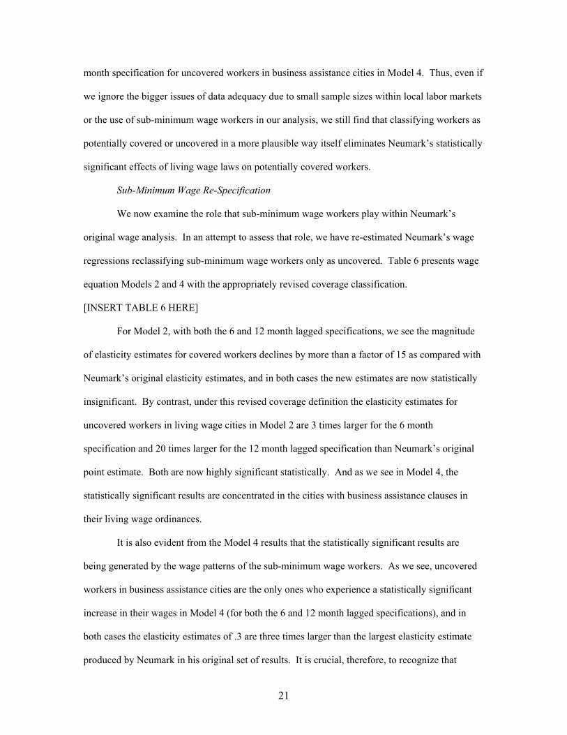
Sub-Minimum Wage Re-Specification

We now examine the role that sub-minimum wage workers play within Neumark’s

original wage analysis. In an attempt to assess that role, we have re-estimated Neumark’s wage

regressions reclassifying sub-minimum wage workers only as uncovered. Table 6 presents wage

equation Models 2 and 4 with the appropriately revised coverage classification.


For Model 2, with both the 6 and 12 month lagged specifications, we see the magnitude

of elasticity estimates for covered workers declines by more than a factor of 15 as compared with

Neumark’s original elasticity estimates, and in both cases the new estimates are now statistically

insignificant. By contrast, under this revised coverage definition the elasticity estimates for

uncovered workers in living wage cities in Model 2 are 3 times larger for the 6 month

specification and 20 times larger for the 12 month lagged specification than Neumark’s original

point estimate. Both are now highly significant statistically. And as we see in Model 4, the

statistically significant results are concentrated in the cities with business assistance clauses in

their living wage ordinances.

It is also evident from the Model 4 results that the statistically significant results are

being generated by the wage patterns of the sub-minimum wage workers. As we see, uncovered

workers in business assistance cities are the only ones who experience a statistically significant

increase in their wages in Model 4 (for both the 6 and 12 month lagged specifications), and in

both cases the elasticity estimates of .3 are three times larger than the largest elasticity estimate

produced by Neumark in his original set of results. It is crucial, therefore, to recognize that

21

almost all of the individuals who now fall into the category of uncovered workers in business

assistance cities are sub-minimum wage workers. It is, furthermore, increasingly clear that that

the wage patterns for sub-minimum wage workers are highly influential in generating Neumark’s

original findings.

But let us consider this issue with still greater specificity. As we have seen in Table 3

and our earlier discussion, covered workers in Neumark’s wage analysis are highly concentrated

geographically, with over half in Los Angeles alone in the business assistance models. We

therefore next pose the question: to what degree can Neumark’s results be explained by the wage

patterns of sub-minimum wage workers in Los Angeles alone? Table 7 presents results that shed

light on this question.


In this table, we have conducted an analysis similar to that presented in Table 6, except

we have reclassified the sub-minimum wage workers in Los Angeles alone as uncovered. In the

specification for Model 2 we see that uncovered workers have large and statistically significant

wage effects in both the 6 and 12 month lagged specifications. The implied elasticities of .17 and

.15, respectively, are larger than those estimated for potentially covered workers in Neumark’s

original specifications, and are highly significant. For our Model 4, we find even larger elasticity

estimates for uncovered workers in business assistance cities, .5 and .47 for the 6 and 12 month

lagged specifications, respectively. In short, Neumark’s results are not robust to the

reclassification of sub-minimum wage workers in Los Angeles from his full national category

into the category of uncovered workers.

Wage Dynamics in Los Angeles

These results lead us to consider what actually is happening with sub-minimum wage

workers in Los Angeles in our sample period given that, by definition, these workers are unlikely

to be receiving mandated wage increases due to the passage of the city’s living wage law. While

a comprehensive treatment of the dynamics of the low-wage labor market in Los Angeles is

22

beyond the scope of this paper, two facts are of primary importance as potential sources of

upward wage pressure. First, along with the state of California as a whole, Los Angeles

experienced dramatic declines in unemployment over the time period used in Neumark’s study.

Figure 1 displays these unemployment rates for both California and the LA-Long Beach PMSA

over the period 1995 to 2000. As the figure shows, the monthly unemployment rate in Los

Angeles declined from a high of 9.1 percent in July 1996 to a low of 4.7 percent in December

2000. Economic theory would suggest that, everything else equal, such a sharp decline in

unemployment will give even low-wage workers increased bargaining power relative to

employers, which in turn should drive up even low-end wages.

[INSERT FIGURE 1 HERE]

A second factor is that California’s minimum wage increased from $4.25 to $5.75 over

1996-1998, and the 12 month lagged value of the Los Angeles living wage rises in close

correspondence with the largest minimum wage increase (in absolute terms), though, of course,

the living wage rate far exceeds the new level for the statewide minimum wage. We can observe

this close relationship in Figure 2, which plots both the 12-month lagged living wage value and

the contemporaneous minimum wage value for Los Angeles from January 1996 – October 2000.

We also plot in Panel A of Figure 2 the mean wage of the lowest decile in Los Angeles. What is

clearly suggested by this figure is that a close correlation exists between changes in the mean

wage and the minimum wage, but not between the mean wage and the living wage. We also see

from Panel B that at no point from January 1996 to October 2000 were any of the workers in the

lowest decile in Los Angeles making a wage close to the living wage after it was passed.

[INSERT FIGURE 2 HERE]

This descriptive evidence suggests that we consider more formally the effects of the

California minimum wage increase and decline in the unemployment rate as factors exerting

upward pressure on wages for sub-minimum wage workers in Los Angeles. We present the

results of this formal exercise in Table 8. To begin with, in column one, we see that we do not

23

find a statistically significant positive effect for the living wage variable, lagged 12 months, as we

had with tests run on the full Neumark sample of bottom decile workers. As in Neumark’s initial

specifications, this equation includes the minimum wage with a 12-month lag, which is also

insignificant. In column two we add the unemployment rate to our model specification, using a

moving average of the current unemployment rate that includes observations three months before

and three months after the current period. This seven-month centered moving average is highly

significant, and the magnitude of its effect is as large as that of the living wage variable, which

unlike the column one results, is statistically significant at the 5 percent level in this specification.

The 12-month lagged minimum wage remains insignificant in this specification as well.

However, as seen in column three, when we specify the unemployment rate variable with a six-

month lag, the unemployment rate variable is still statistically significant at the 10 percent level,

while the living wage variable becomes insignificant. When we specify the unemployment rate

variable with a 12-month lag, as reported in column four, none of the variables presented in Table

8 are significant, and the living wage variable actually become negative, along with the 12-month

lagged value of the minimum wage.


The descriptive evidence in Figure 2 suggested that we also consider the minimum wage

effects more carefully than we have done thus far, as we have up to this point relied on the 12-

month lagged value of the minimum wage as the only specification for this variable. In all of

Neumark’s models, the minimum wage is included with a lag period identical to the lag for the

living wage variable. However there are good reasons to believe that unlike living wage

ordinances, minimum wage laws do not entail the same lag in implementation. For one thing, the

minimum wage is a long-standing labor market institution, and an increase does not require the

long implementation process that has been the case with living wage ordinances. Minimum wage

increases also do not depend on city service contracting cycles, as do some living wage

ordinances. Thus, minimum wage changes can be expected to take effect relatively quickly.

24

This all points towards the inclusion of the contemporaneous minimum wage as an

alternative specification in our estimates, which we do in columns 5-7 of Table 8. In column 5,

as in column 2, we see that with the current unemployment rate variable included, the

unemployment variable is significant and with the appropriate sign while the living wage and

minimum wage variables are both insignificant. In column 6 however, when the unemployment

rate is lagged six months, the 12 month lagged living wage variable becomes insignificant and

drops dramatically in magnitude. Moreover, the contemporaneous minimum wage increases

dramatically in magnitude, and becomes statistically significant at the five percent level. When

we include unemployment lagged 12 months, only the contemporaneous minimum wage is

significant (at the five percent level) with an elasticity of 0.78. These results are broadly similar

for the living wage variable lagged 6 months.

Overall, these results are consistent with the descriptive evidence in showing the

importance of the decline in the unemployment rate and the rise in the minimum wage in pulling

up the wages of sub-minimum wage workers in Los Angeles. At the very least, we can conclude

that the living wage is not robust as an explanatory variable on wages for this sample of workers,

while the unemployment rate is highly robust in its explanatory power. The contemporaneous

minimum wage is also more consistently a significant factor than the living wage lagged 12

months. The broad conclusion, then, is that the rise in wages for LA’s sub-minimum wage

workers is driven substantially by changes in the unemployment rate in the region and, somewhat

less clearly, by the California minimum wage changes. The wages of LA’s sub-minimum wage

market are not being driven to a statistically significant extent, much less a substantively

significant extent, by in the LA living wage. This broad conclusion is important, in turn, for the

overall interpretation of Neumark’s study, since, as we have seen, the effects of living wage

ordinances throughout the United States are themselves dependent on including LA’s sub-

minimum wage workers in his sample.

25

5. Re-Examining Neumark’s Employment Result

We now turn to a brief examination of Neumark’s employment results in light of the

concerns raised in Section 3 and the examination of his wage results in Section 4. The first major

issue we address is whether Neumark’s employment effects are in fact caused by workers likely

to be covered by living wage laws. As noted above, Neumark’s approach to estimating

employment effects involves incorporating a large number of individuals who are not currently in

the labor force, and therefore who do not possess identifying information on wages or sector of

the economy in which they work. Including these individuals outside the labor force in his

employment analysis means that Neumark is unable to reproduce the “potentially covered” and

“potentially uncovered” classifications that were the centerpiece of his wage analysis. However,

drawing upon Neumark, we develop here an approach which does allow us to retain this crucial

covered/uncovered distinction. This approach proceeds from the fact that the Current Population

Survey incorporates information on sector of activity for all individuals who have been in the

labor force at sometime in the past year, even if they were out of the labor force at the time they

were surveyed. By restricting our sample to only those individuals who currently are or have

been in the labor force in the last year, we are then able to preserve the covered/uncovered

distinction. This restriction, moreover, is appropriate in substantive terms, since it is over the set

of individuals with at least some marginal attachment to the labor market that we should expect to

see any employment effects from living wage laws.

In Table 9 we estimate three employment models, using the specifications from wage

Models 1-3, with the restricted sample discussed above. In the first panel, we see that for Model

1, when the living wage variable is lagged 12 months it is statistically significant at the 5 percent

level, with a magnitude very close to the -5.62 estimate seen in Table 2A. This suggests that

while we are restricting our sample to those who have been at least marginally attached to the

labor market within the year of the sample, we are still not making a significant empirical

departure from Neumark’s original analysis.

26


In the second panel, we find evidence still consistent with Neumark’s findings, namely a

negative and statistically significant coefficient (at the 10 percent level) of -6.65 for the living

wage variable for covered workers lagged 12 months. Interestingly, when we separate cities into

those with business assistance laws, versus those with contractor-only laws—i.e. Model 3,

presented in panel 3 of Table 9—we find that the living wage does not have a statistically

significant effect on the employment status of our sample. It should be noted, however, that

although neither the living wage variables for contractor-only nor business-assistance cities are

statistically significant at conventional levels, the business assistance living wage variable is

significant at a 15% threshold, and therefore could arguably be interpreted as supportive of

Neumark’s model with the reduced sample size.

It is at this stage that our ability to separate out covered from uncovered workers becomes

important. Following our approach from the preceding section, in the bottom panel of Table 9 we

adjust Neumark’s classification of workers as potentially covered and uncovered to reflect the

actual application of living wage laws by cities that have business assistance provisions. In other

words, as with our approach with the wage models, we reclassify workers outside the service

sector as uncovered, reflecting information on actual implementation of living wage laws

provided to us by city officials. As seen in the fourth panel, when this adjustment is made, there

is no statistically significant effect for covered workers, and none for uncovered workers either at

conventional levels. Uncovered workers do display a negative and statistically significant

coefficient for the living wage lagged 12 months if we consider the significance threshold to be

15% instead of 10%. Overall, we again find that Neumark’s results are not robust to alternative

specifications that are informed by the actual experiences with implementing living wage laws.

6. Concluding Remarks

This critical appraisal of David Neumark’s 2002 study challenges his argument that

living wage ordinances, particularly those covering business-assistance living wage ordinances,

27

increase wages for a far larger proportion of low-wage workers than has been previously

estimated. We also challenge Neumark’s finding that living wage ordinances cause

disemployment.

On methodological grounds we have demonstrated why the Current Population Survey is

not an appropriate dataset for analyzing either the wage or employment effects of living wage

laws. We have also argued, on methodological grounds alone, that Neumark’s truncated OLS

regressions are vulnerable to problems of sample selection bias. The results we obtained through

our quantile regression specification certainly, at the very least, raises concerns about the

robustness of Neumark’s results using his truncated OLS methodology. But even accepting

Neumark’s truncated OLS methodology on its own terms, we demonstrate that his statistically

significant results hinge on the way in which he treats workers earning below the minimum wage,

as well as how he defines covered workers in business-assistance living wage cities. We show

that through classifying sub-minimum wage workers as uncovered, as opposed to Neumark’s

category “potentially covered,” Neumark’s statistically significant wage results are invalidated

for “potentially covered” workers. Moreover, based on interviews with city staff in the cities in

question, we have demonstrated that Neumark’s approach to defining “potentially covered”

workers in cities with business assistance ordinances drastically overstates the number of workers

likely to have received mandated wage increases through existing living wage laws. We have

also shown that once Neumark’s definition of “potentially covered” workers is corrected for this

misclassification, we find no statistically significant effect of living wage ordinances on wages or

employment for covered workers. Finally, we have shown that Neumark’s original results rest on

a sample weighted heavily toward just sub-minimum wage workers in Los Angeles. When sub-

minimum wage workers in Los Angeles alone are reclassified as uncovered, Neumark’s putative

“living wage effects” are again invalidated.

The overall conclusion that we reach is clear: David Neumark’s analysis of the effects of

living wage laws in the United States has produced no results that stand up to the scrutiny of this

28

critical replication exercise. Of course, our results do not speak to the broader substantive

question as to how living wage laws have affected low-wage workers in terms of either their

wages or their employment opportunities. But we expect that many researchers will continue to

make progress in addressing these substantive questions, which are, of course, the central matters

of concern for understanding how living wage laws are affecting the lives of low-wage workers in

the United States.

29

References Apney, Carol, City of Detroit, Contract Department. Interview 10/30/01 with Mark Brenner, on

file with authors. Card, David and Alan Krueger (1995) Myth and Measurement: The New Economics of the Minimum

Wage, Princeton, NJ: Princeton University Press Eissa, Nada and Hilary Williamson Hoynes (1998) “The Earned Income Tax Credit and the

Labor Supply of Married Couples,” NBER Working Paper No. 6856. Eissa, Nada and Jeffery B. Liebman (1996) “Labor Supply Response to the Earned Income Tax

Credit,” Quarterly Journal of Economics, Vol. 111, No. 2, pp. 605-637. Enman, Vivian, City of Oakland. Interview 10/30/01 with Mark Brenner, on file with authors. Gibson, June, City of Los Angeles, CAO’s Office. Interview 10/18/01 with Mark Brenner, on

file with authors. Greyson, Nina, City of San Jose. Interview 10/15/01 with Mark Brenner, on file with authors. Jacobson, Trey, City of San Antonio, Redevelopment Office. Interview 10/29/01 with Mark

Brenner, on file with authors. Heckman, James J. (1979) “Sample Selection Bias as a Specification Error,” Econometrica, 47:1, January,

pp. 153-61. Katz, Lawrence and Alan Krueger (1992) “The Effects of the Minimum Wage on the Fast Food Industry,”

Industrial and Labor Relations Review, 46: 6-21. Killingsworth, Mark R. and James J. Heckman (1986), “Female Labor Supply: A Survey” in

Orley Ashenfelter and Richard Layard, eds. Handbook of Labor Economics. Vol. 1. Amsterdam: North-Holland, pages 103-204.

Koenker, Roger and Kevin F. Hallock (2001) “Quantile Regression,” Journal of Economic Perspectives,

15:4, Fall, pp. 143-56.

Maddala, G.S. (1983) Limited Dependent and Qualitative Variables in Econometrics, Cambridge, UK: Cambridge University Press.

Neumark, David (2002) “How Living Wage Laws Affect Low Wage Workers and Low-Income

Families,” Public Policy Institute of California Report #156. Niedt, Christopher, Ruiters, Greg, Wise, Dana and Schoenberger, Erica (1999) "The Effects of

the Living Wage in Baltimore," Working Paper # 119, Washington, D.C.: Economic Policy Institute.

Pollin, Robert and Mark D. Brenner (2000), Economic Analysis of Santa Monica Living Wage

Proposal. Political Economy Research Institute, Research Report Number 2. Pollin, Robert and Stephanie Luce (2000), The Living Wage: Building a Fair Economy. New

York, NY: The New Press. Reich, Michael, Peter Hall and Fiona Hsu (1999) “Living Wages and the San Francisco

Economy: The Benefits and Costs,” Institute for Industrial Relations, University of California-Berkeley, June.

30

31

Robbins, Kent, City of Minneapolis, MCDA. Interview 10/23/01 with Mark Brenner, on file with

authors.

Centile range: <=10 10-25 25-50 50-75

Specification 1: -0.53 0.27 0.95 -0.03Living Wage (2.23) (1.62) (1.65) (1.63)

Specification 2: 1.91 0.84 2.22 0.34Living wage, 6-month lag (2.25) (1.70) (1.76) (1.79)

Specification 3: 6.95** 0.93 -0.01 -1.08Living wage, 12-month lag (2.40) (1.78) (1.85) (1.92)

Unweighted Ns: 34,435 42,912 71,135 72,737

Uncovered Covered Uncovered CoveredWorkers Workers Workers Workers

Centile range:

Specification 1: -4.99* 2.11 -1.02 1.23Living Wage (2.97) (2.53) (1.82) (1.78)

Specification 2: -4.62 5.66** -1.09 1.98Living wage, 6-month lag (3.07) (2.56) (1.92) (1.89)

Specification 3: 0.61 10.61** -1.28 2.26Living wage, 12-month lag (3.49) (2.72) (2.07) (2.00)

Unweighted Ns:

Contractor Business Contractor BusinessOnly Assistance Only Assistance

Living Wage Living Wage Living Wage Living WageCentile range:

Specification 1: -4.50 1.78 -2.82 2.15Living Wage (3.45) (2.76) (2.30) (2.09)

Specification 2: -5.22 5.83** -2.21 2.64Living wage, 6-month lag (3.66) (2.66) (2.38) (2.21)

Specification 3: 0.50 10.54** -1.92 2.72Living wage, 12-month lag (4.02) (2.78) (2.49) (2.31)

Unweighted Ns:

<=10 10-25

42,638

42,912

Table 1A: Effects of Living Wage Laws on Wages,Alternative Classifications of Workers and Living Wage Laws

Replicating results from Neumark 2002

34,435

<=10 10-25

Model 1: All Living Wage Laws

Model 2: Potentially Covered and Uncovered Workers

Model 3: Contractor and Business Assistance Living Wage Laws

34,196

Notes: These results are identical to those in Neumark (2002), Tables 5.3, 5.5, and 5.6. The dependent variable is log wages. Estimated coefficients have been multiplied by 100. Standard errors reported in parentheses are robust to heteroskedasticity and non-independence within city-month cells. A city's observations are included in the sample in a particular month and year if it has at least 25 observations for that particular month and year. See text for other controls included in the regression. * indicates statistical significance at the .10 level. ** indicates statistical significance at the .05 level.


Centile range:

Specification 2: -6.18* 0.21 -0.24 6.52**Living wage, 6-month lag (3.67) (6.53) (5.91) (2.72)

Specification 3: -0.52 6.46 4.72 11.21**Living wage, 12-month lag (4.11) (7.26) (6.05) (2.88)

Unweighted N: 34,196

Contractor Living Wage Laws Business Assistance Living Wage Laws

<=10

Table 1B: Effects of Living Wage Laws on Wages, Potentially Covered and Uncovered Workers Under Business Assistance and Contractor Living Wage Laws

An Extension of Models 2 and 3Model 4

Notes: See notes to Table 1A. * indicates statistical significance at the .10 level. ** indicates statistical significance at the .05 level.

Centile range: <=10 10-25 25-50 50-75

Specification 1: -1.77 0.02 2.58** 1.79*Living Wage (2.14) (1.81) (1.18) (1.04)

Specification 2: -3.22 1.16 2.31* 1.32Living wage, 6-month lag (2.26) (1.88) (1.24) (1.08)

Specification 3: -5.62** 1.62 1.55 2.44**Living wage, 12-month lag (2.45) (2.02) (1.31) (1.16)

Unweighted Ns: 83,326 118,541 197,477 199,703



Specification 1: -3.26 -0.81 0.59 -0.34Living Wage (3.19) (2.73) (2.75) (2.26)

Specification 2: -5.49 -1.74 1.03 1.24Living wage, 6-month lag (3.40) (2.90) (2.85) (2.36)

Specification 3: -5.26 -5.88* 1.45 1.74Living wage, 12-month lag (3.79) (3.06) (3.06) (2.54)

Unweighted Ns:

Table 2A: Effects of Living Wage Laws on Employment,Alternative Classifications of Living Wage Laws

Replicating results from Neumark 2002

83,326 118,541

<=10 10-25



Notes: These results are identical to those in Neumark (2002), Tables 6.1 and 6.2. The dependent variable is employment status. Estimated coefficients have been multiplied by 100. Standard errors reported in parentheses are robust to heteroskedasticity and non-independence within city-month cells. A city's observations are included in the sample in a particular month and year if it has at least 25 observations for that particular month and year. See text for other controls included in the regression. * indicates statistical significance at the .10 level. ** indicates statistical significance at the .05 level.

Centile range: <=10 10-25 25-50 50-75

Specification 1: -1.06 -0.01 2.50** 1.75*Living Wage (2.15) (1.84) (1.19) (1.05)

Specification 2: -2.51 0.97 2.35* 1.44Living wage, 6-month lag (2.29) (1.91) (1.25) (1.09)

Specification 3: -4.80* 1.46 1.71 2.67**Living wage, 12-month lag (2.48) (2.05) (1.32) (1.17)

Unweighted Ns: 78,779 112,555 187,605 189,442



Specification 1: -2.58 -0.12 0.56 -0.37Living Wage (3.23) (2.74) (2.83) (2.27)

Specification 2: -4.64 -1.19 0.69 1.14Living wage, 6-month lag (3.47) (2.90) (2.94) (2.38)

Specification 3: -3.99 -5.34* 1.34 1.55Living wage, 12-month lag (3.91) (3.07) (3.17) (2.56)

Unweighted Ns: 78,779 112,555

Table 2B: Effects of Living Wage Laws on Employment,Alternative Classifications of Living Wage Laws

Sample Restricted to Cities in Wage Analysis

<=10 10-25



Notes: The dependent variable is employment status. Estimated coefficients have been multiplied by 100. Standard errors reported in parentheses are robust to heteroskedasticity and non-independence within city-month cells. A city's observations are included in the sample if it appeared in the wage analysis sample. See text for other controls included in the regression. * indicates statistical significance at the .10 level. ** indicates statistical significance at the .05 level.

Panel A: Wage Analysis

City Unwtd. N Wtd. % Unwtd. N Wtd. % Unwtd. N Wtd. %

Los Angeles 1,196 27.5 1,136 49.1 1,196 52.4Minneapolis 369 10.4 344 18.2 369 19.8Detroit 230 5.0 215 8.7 230 9.5Oakland 106 4.2 94 7.0 106 7.9San Antonio 79 2.6 73 4.5 79 4.9San Jose 69 2.6 58 4.2 69 5.0Hartford 9 0.3 7 0.4 9 0.5Chicago 476 10.4 44 1.9 -- --Baltimore 325 12.6 23 1.7 -- --Milwaukee 250 8.0 25 1.6 -- --Durham 96 2.3 31 1.4 -- --Boston 157 3.5 20 0.8 -- --Portland 360 8.4 13 0.6 -- --Dayton 95 2.1 1 0.0 -- --Jersey City 15 0.3 1 0.0 -- --

Total 3,832 100 2,085 100 2,058 100

Panel B: Employment Analysis

City Unwtd. N Wtd. % Unwtd. N Wtd. %

Los Angeles 2,348 26.3 2,348 53.4Minneapolis 592 8.2 592 16.6Detroit 472 5.1 472 10.4Oakland 218 4.2 218 8.5San Antonio 147 2.4 147 4.8San Jose 119 2.3 119 4.7Hartford 21 0.3 21 0.5Madison 20 0.3 20 0.6Tucson 17 0.2 17 0.4Duluth 3 0.0 3 0.1Baltimore 645 12.2 -- --Boston 400 4.3 -- --Chicago 1,109 12.2 -- --Dayton 168 1.8 -- --Jersey City 203 2.2 -- --Milwaukee 434 6.7 -- --New Haven 109 1.4 -- --Portland 617 7.4 -- --Durham 216 2.6 -- --

Total 7,858 100 3,957 100

All Living Wage Laws Business Assistance Cities

Notes: In Model 1, affected workers are those workers who live in a city with a living wage ordinance in effect (lagged 12 months). In Model 2, affected workers are those workers who live in a city with a living wage ordinance in effect (lagged 12 months) and are classified as "potentially covered" according to their industry affiliation. In Model 3, affected workers are those workers who live in a city with a business-assistance type living wage ordinance in effect (lagged 12 months).

All Living Wage Laws Covered Workers Business Assistance Cities

Model 1 Model 3

Table. 3: Composition of Affected Workers in the Lowest Decile12-Month Lagged Living Wage Specifications

Model 1 Model 2 Model 3

Table 4: Estimating the Effects of Living Wage Laws on WagesReplicating Neumark's Models 1-3 Utilizing Quantile Regression

Model 1: All Living Wage LawsQuantile Specified: 10th

Living wage, 12-month lag 0.74(1.35)

N 291,743

Model 2: All Living Wage LawsUncovered CoveredWorkers Workers

Quantile Specified: 10th

Living wage, 12-month lag 0.48 3.04*(2.43) (1.60)

N 291,743

Model 3: Contractor and Business Assistance Living WageContractor Business

Only AssistanceLiving Wage Living Wage

Quantile Specified: 10th

Living wage, 12-month lag -0.15 1.09(2.70) (1.21)

N 291,743

Notes: These results are estimated using quantile regression for the 10th centile of the wage distribution. Standard errors are bootstrapped to address heteroskedasticity. * indicates statistical significance at the .10 level. ** indicates statistical significance at the .05 level.

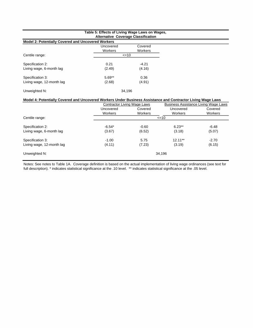
Uncovered CoveredWorkers Workers

Centile range:

Specification 2: 0.21 -4.21Living wage, 6-month lag (2.49) (4.16)

Specification 3: 5.69** 0.36Living wage, 12-month lag (2.68) (4.91)

Unweighted N:


Centile range:

Specification 2: -6.54* -0.60 6.23** -6.48Living wage, 6-month lag (3.67) (6.52) (3.18) (5.07)

Specification 3: -1.00 5.75 12.11** -2.70Living wage, 12-month lag (4.11) (7.23) (3.19) (6.15)

Unweighted N:

<=10

34,196

34,196

Model 4: Potentially Covered and Uncovered Workers Under Business Assistance and Contractor Living Wage LawsContractor Living Wage Laws Business Assistance Living Wage Laws

Table 5: Effects of Living Wage Laws on Wages, Alternative Coverage Classification


<=10

Notes: See notes to Table 1A. Coverage definition is based on the actual implementation of living wage ordinances (see text for full description). * indicates statistical significance at the .10 level. ** indicates statistical significance at the .05 level.


Centile range:



Unweighted N:


Centile range:

Specification 2: -0.56 5.74 30.27** 1.89Living wage, 6-month lag (2.46) (3.88) (4.83) (2.30)


Unweighted N:

<=10

34,196

34,196


Table 6: Effects of Living Wage Laws on Wages, Subminimum Wage Workers Classified as Uncovered


<=10

Notes: See notes to Table 1A. Subminimum wage workers who were previously classified as covered are classified as uncovered here, along with workers classified as uncovered based on the industry affiliation. * indicates statistical significance at the .10 level. ** indicates statistical significance at the .05 level.


Centile range:

Specification 2: 16.54** -0.43Living wage, 6-month lag (2.99) (2.15)

Specification 3: 15.03** -0.22Living wage, 12-month lag (3.23) (2.38)

Unweighted N:


Centile range:

Specification 2: -0.13 -0.14 49.76** 2.43Living wage, 6-month lag (2.43) (4.71) (5.36) (2.19)


Unweighted N:

<=10

34,196

34,196


Table 7: Effects of Living Wage Laws on Wages, Los Angeles Subminimum Wage Workers Classified as Uncovered


<=10

Notes: See notes to Table 1A. Los Angeles subminimum wage workers who were previously classified as covered are classified as uncovered here, along with workers classified as uncovered based on the industry affiliation. * indicates statistical significance at the .10 level. ** indicates statistical significance at the .05 level.

Figure 1 - Unemployment Rate in California and Los Angeles: 1995-2000(Not Seasonally Adjusted)

3

4

5

6

7

8

9

10

Jan-9

5Apr-

95Ju

l-95

Oct-95

Jan-9

6Apr-

96Ju

l-96

Oct-96

Jan-9

7Apr-

97Ju

l-97

Oct-97

Jan-9

8Apr-

98Ju

l-98

Oct-98

Jan-9

9Apr-

99Ju

l-99

Oct-99

Jan-0

0Apr-

00Ju

l-00

Oct-00

Month

Per

cen

t

CALA

Panel A - Comparing Minimum and Living wages to 10th Decile Average Wages.

Panel B - Comparing Minimum and Living wages to 10th Decile Maximum Wages

$3.00

$4.00

$5.00

$6.00

$7.00

$8.00

Jan-9

6Apr-

96Ju

l-96

Oct-96

Jan-9

7Apr-

97Ju

l-97

Oct-97

Jan-9

8Apr-

98Ju

l-98

Oct-98

Jan-9

9Apr-

99Ju

l-99

Oct-99

Jan-0

0Apr-

00Ju

l-00

Oct-00

Cu

rren

t $

Living Wage,Lagged 12 months

California Minimum Wage

10th Decile Mean Wage

Figure 2. Los Angeles Wage Trends, 1996-2000

$3.00

$4.00

$5.00

$6.00

$7.00

$8.00

Jan-9

6Apr-

96Ju

l-96

Oct-96

Jan-9

7Apr-

97Ju

l-97

Oct-97

Jan-9

8Apr-

98Ju

l-98

Oct-98

Jan-9

9Apr-

99Ju

l-99

Oct-99

Jan-0

0Apr-

00Ju

l-00

Oct-00

Cu

rren

t $

Living Wage,Lagged 12 months

California Minimum Wage

10th Decile Maximum Wage

Table 8: Explaining Wages for Subminimum Wage Workers in Los Angeles

Model 1 (1) (2) (3) (4) (5) (6) (7)

Centile range: <=10 <=10 <=10 <=10 <=10 <=10 <=10

Unemployment Rate - -22.01** - - -20.69** - -(7 month moving average, centered) (7.45) (7.02)

Unemployment Rate, lagged 6 months - - -10.06** - - -10.26** -(7 month moving average, centered) (3.64) (3.35)

Unemployment Rate, lagged 12 months - - - -3.23 - - -5.84(7 month moving average, centered) (5.95) (5.83)

Minimum Wage, current - - - - 12.49 69.82* 76.16**(35.15) (37.21) (36.17)

Minimum Wage, lagged 12 months -14.9 -43.49 -53.91 -19.33 -39.66 -42.84 -10.02(38.65) (36.52) (39.17) (38.33) (38.69) (38.83) (36.40)

Living Wage, lagged 12 months 1.03 23.71** 4.35 -2.48 20.53* -5.73 -16.38(8.09) (10.44) (7.12) (11.08) (11.74) (9.14) (12.69)

Unweighted N: 845 845 845 845 845 845 845

Notes: See notes to Table 1A. * indicates statistical significance at the .10 level. ** indicates statistical significance at the .05 level.

Alternative Samples and Classifications

Centile range: <=10

Specification 1: -0.65Living wage (2.50)

Specification 2: -1.58Living wage, 6-month lag (2.55)

Specification 3: -5.38**Living wage, 12-month lag (2.74)

Unweighted N: 47,759


Centile range:

Specification 1: -1.06 -1.35Living wage (3.28) (2.96)

Specification 2: -2.26 -3.16Living wage, 6-month lag (3.40) (3.21)

Specification 3: -5.70 -6.65*Living wage, 12-month lag (3.83) (3.55)

Unweighted N:

Contractor BusinessOnly Assistance

Centile range:

Specification 1: -2.42 0.49Living wage (3.58) (3.26)



Unweighted N:

or NILF and worked in last year]


Centile range:

Specification 1: -0.47 -1.45Living wage (2.62) (4.71)



Unweighted N:

47,759

Model 2 - Corrected Classification, New Sample [only those in the labor force or

<=10

46,133

<=10

46,133

Model 3, New Sample [only those in the labor force or NILF and worked last year]

<=10

Table 9: Effects of Living Wage Laws on Employment,

Model 1, New Sample [only those in the labor force or NILF and worked last year]

Model 2: Potentially Covered and Uncovered Workers, Neumark's Classification - New Sample [only those in the labor force or NILF and worked last year]

Notes: The dependent variable is employment status. Estimated coefficients have been multiplied by 100. Standard errors reported in parentheses are robust to heteroskedasticity and non-independence within city-month cells. A city's observations are included in the sample if it appeared in the wage analysis sample. See text for other controls included in the regression. * indicates statistical significance at the .10 level. ** indicates statistical significance at the .05 level.

Measuring the Impact of Living Wage Laws: A Critical Appraisal of David Neumark's How Living Wage...

Documents

Transcript of Measuring the Impact of Living Wage Laws: A Critical Appraisal of David Neumark's How Living Wage...