MODELING LIQUID EVAPORATION AND USING ...

ABSTRACT

Title of Thesis: MODELING LIQUID EVAPORATION AND

USING MOLECULAR DYNAMICS

SIMULATION TO ESTIMATE DIFFUSION

COEFFICIENTS AND RELATIVE

SOLVENT DRYING TIMES

Rehan Choudhary, Master of Science, 2017

Thesis Directed By: Associate Professor and Graduate Program

Director, Jeffery Klauda, Department of

Chemical and Biomolecular Engineering

In this thesis, the Simultaneous Mass and Energy Evaporation (SM2E) model is

presented. This model is based on theoretical expressions for mass and energy transfer

and can be used to estimate evaporation rates for pure liquids as well as liquid mixtures

at laminar, transition, and turbulent flow conditions. However, due to limited

availability of evaporation data, the model has so far only been tested against data for

pure liquids and binary mixtures. The model can take evaporative cooling into account.

For the case of isothermal evaporation, the model becomes a mass transfer-only model.

Also in this thesis, molecular dynamics (MD) simulation is used to estimate gas phase

diffusion coefficients based on mean-square displacement methods and results are

compared with Chapman-Enksog theory. MD simulation is also used to model

evaporation of solvents into air and relative solvent drying times based on simulation

are compared with measured values.

MODELING LIQUID EVAPORATION AND USING MOLECULAR

DYNAMICS SIMULATION TO ESTIMATE DIFFUSION COEFFICENTS AND

RELATIVE SOLVENT DRYING TIMES

by

Rehan Choudhary

Thesis submitted to the Faculty of the Graduate School of the

University of Maryland, College Park, in partial fulfillment

of the requirements for the degree of

Master of Science

2017

Advisory Committee:

Professor Jeffery Klauda, Chair

Professor Panagiotis Dimitrikopoulos

Professor Nam Sun Wang

© Copyright by

Rehan Choudhary

2017

ii

Acknowledgements

I decided to pursue graduate studies in engineering after having worked in

industry and government for about 10 years. In addition to being a son and brother, I

was also a husband and father at this point in my life.

We are all influenced by the environments that we are exposed to as we grow

and come of age. And from these early years, we carry with us certain habits along

with their strengths and weaknesses. But these early years need not determine the

remainder of our lives and if we are fortunate, those very same early years will also

have equipped us with enough flexibility to understand that we can chart a different

path, our own path, if we so choose.

My years as a graduate student were well spent. I didn’t just take graduate

classes and pursue research endeavors that were already decided for me. I embraced

the uncertainty that comes with having to structure your own research and I also used

these years to learn how to learn without the structure of a classroom.

I want to express my gratitude to my parents for equipping me with that much

needed flexibility during my early years. To my siblings, we are all on our own paths

at this point in our lives. It is my hope the aspirations that have driven us apart will

also join us once again. To my wife, I am blessed to be walking this path alongside

you. And to my children, love and always be kind to your mother and remember that

we shall return to God.

iii

There were times when I thought that I may not be able to complete my graduate

studies and I am fortunate this is not the case. For this, I want to thank my advisor (Dr.

Klauda) for his guidance, patience, and flexibility in working with a part-time graduate

student such as myself during these past few years. And I also want to thank Dr.

Dimitrikopoulos and Dr. Wang for the enthusiasm they expressed in their willingness

to serve on my thesis committee and for reviewing this work.

iv

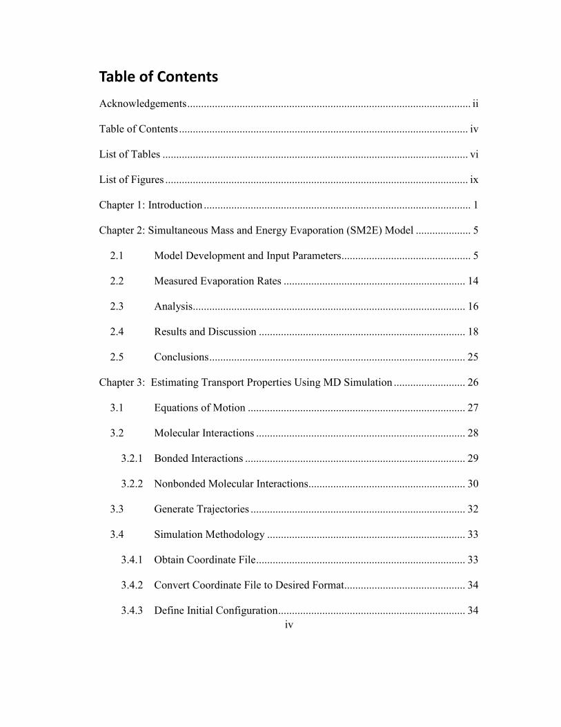
Table of Contents

Acknowledgements ....................................................................................................... ii

Table of Contents ......................................................................................................... iv

List of Tables ............................................................................................................... vi

List of Figures .............................................................................................................. ix

Chapter 1: Introduction ................................................................................................. 1

Chapter 2: Simultaneous Mass and Energy Evaporation (SM2E) Model .................... 5

2.1 Model Development and Input Parameters ............................................... 5

2.2 Measured Evaporation Rates .................................................................. 14

2.3 Analysis................................................................................................... 16

2.4 Results and Discussion ........................................................................... 18

2.5 Conclusions ............................................................................................. 25

Chapter 3: Estimating Transport Properties Using MD Simulation .......................... 26

3.1 Equations of Motion ............................................................................... 27

3.2 Molecular Interactions ............................................................................ 28

3.2.1 Bonded Interactions ................................................................................ 29

3.2.2 Nonbonded Molecular Interactions......................................................... 30

3.3 Generate Trajectories .............................................................................. 32

3.4 Simulation Methodology ........................................................................ 33

3.4.1 Obtain Coordinate File ............................................................................ 33

3.4.2 Convert Coordinate File to Desired Format............................................ 34

3.4.3 Define Initial Configuration .................................................................... 34

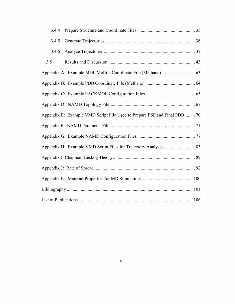
v

3.4.4 Prepare Structure and Coordinate Files .................................................. 35

3.4.5 Generate Trajectories .............................................................................. 36

3.4.6 Analyze Trajectories ............................................................................... 37

3.5 Results and Discussion ........................................................................... 43

Appendix A: Example MDL Molfile Coordinate File (Methane) ............................. 63

Appendix B: Example PDB Coordinate File (Methane) ........................................... 64

Appendix C: Example PACKMOL Configuration Files ........................................... 65

Appendix D: NAMD Topology File .......................................................................... 67

Appendix E: Example VMD Script File Used to Prepare PSF and Final PDB ......... 70

Appendix F: NAMD Parameter File .......................................................................... 71

Appendix G: Example NAMD Configuration Files .................................................. 77

Appendix H: Example VMD Script Files for Trajectory Analysis............................ 83

Appendix I: Chapman-Enskog Theory ....................................................................... 89

Appendix J: Rate of Spread ....................................................................................... 92

Appendix K: Material Properties for MD Simulations ............................................ 100

Bibliography ............................................................................................................. 101

List of Publications ................................................................................................... 106

vi

List of Tables

Table 1: UNIFAC activity coefficients for relevant binary mixtures; activity

coefficients were estimated at a temperature of 298 K using XLUNIFAC version 1.0

(Randhol, et al., 2014); relative to experimental measurements, the error in the

UNIFAC model is approximated to be ± 26% (UNIFAC Consortium); D = dilute

component; A = abundant component; x = mole fraction. ......................................... 12

Table 2: Antoine equation coefficients for relevant substances (Knovel, 2013; Poling,

et al., 2001); data for Heat of Vaporization (NIST, 2014; Poling, et al., 2001; Smith, et

al., 2005); for Xylene, used property values for m-Xylene since commercial Xylene

can contain up to 65% m-Xylene (U.S. EPA, 2014) and m-Xylene, o-Xylene, p-Xylene

have similar vapor pressures and heats of vaporization.............................................. 13

Table 3: Evaporation rates were measured for 16 different liquid chemicals in a test

duct; all chemicals were reported as being reagent grade; evaporation rates were

measured gravimetrically (Braun, et al., 1989). .......................................................... 15

Table 4: A total of 17 evaporation rates were reported (Olsen, et al., 1995); four (4)

for pure liquids; thirteen (13) for components in binary mixtures; all chemicals were

reported as being of high purity (greater than 99.5% by weight); the evaporation rate

for Water in the Ethanol/Water binary mixture was not reported; D = dilute component;

A = abundant component; x = mole fraction; binary mixtures were maintained at

constant composition during testing. .......................................................................... 16

Table 5: Optimized model correction factors at different air flow conditions.......... 20

Table 6: Coordinate files for these chemicals were obtained from ChemSpider. ..... 26

Table 7: MD simulation was used to estimate self-diffusion coefficients for the

following chemicals; the simulation temperature, number of molecules (�), and

simulation box dimensions are also listed; the density and temperature correspond

approximately to a pressure of 1 atm; simulations were run for 2 ns. ........................ 46

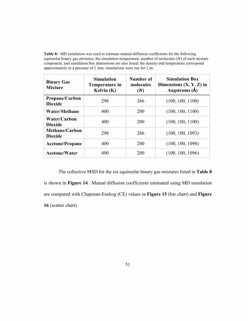
Table 8: MD simulation was used to estimate mutual-diffusion coefficients for the

following equimolar binary gas mixtures; the simulation temperature, number of

molecules (�) of each mixture component, and simulation box dimensions are also

listed; the density and temperature correspond approximately to a pressure of 1 atm;

simulations were run for 2 ns. ..................................................................................... 51

Table 9: MD simulation was used to estimate relative solvent drying times for the

following chemicals; the simulation temperature, number of molecules of the

evaporating chemical (�1), number of Air molecules (�2), and simulation box

vii

dimensions are also listed; the density and temperature correspond approximately to a

pressure of 1 atm. ........................................................................................................ 58

Table 10: Average rate of solvent spread during liquid evaporation as measured from

MD simulation; see Figure 8 for an illustration; relative solvent drying times are

estimated based on the average rate of spread as shown in Equation (39). ................ 59

Table A - 1: Contents of a Methane MDL Molfile obtained from ChemSpider. ..... 63

Table B - 1: Contents of a Methane PDB file obtained from Open Babel. .............. 64

Table C - 1: PACKMOL input file for estimating diffusion for a Methane-Carbon

Dioxide gas mixture at approximately 298 K and 1 atm; all dimensions are in

Angstroms. .................................................................................................................. 65

Table C - 2: PACKMOL input file for estimating evaporation of an Acetone-Air

system at approximately 296 K and 1 atm; all dimensions are in Angstroms. ........... 66

Table D - 1: NAMD topology file used for MD simulations.................................... 67

Table E - 1: VMD script file used to prepare PSF and final PDB files for a Methane-

Carbon Dioxide system; the PDB file that is being modified by this script is the one

generated with the PACKMOL input file shown in Table C - 1. .............................. 70

Table F - 1: NAMD parameter file used for MD simulations. ................................. 71

viii

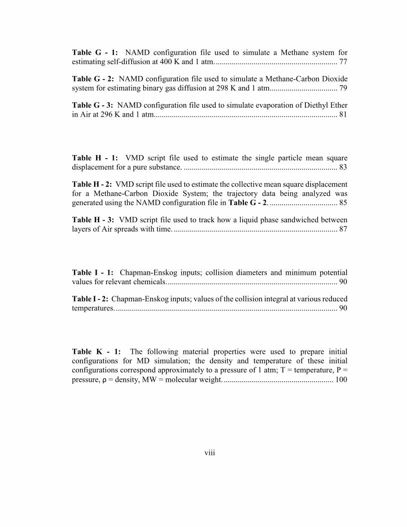
Table G - 1: NAMD configuration file used to simulate a Methane system for

estimating self-diffusion at 400 K and 1 atm. ............................................................. 77

Table G - 2: NAMD configuration file used to simulate a Methane-Carbon Dioxide

system for estimating binary gas diffusion at 298 K and 1 atm.................................. 79

Table G - 3: NAMD configuration file used to simulate evaporation of Diethyl Ether

in Air at 296 K and 1 atm............................................................................................ 81

Table H - 1: VMD script file used to estimate the single particle mean square

displacement for a pure substance. ............................................................................. 83

Table H - 2: VMD script file used to estimate the collective mean square displacement

for a Methane-Carbon Dioxide System; the trajectory data being analyzed was

generated using the NAMD configuration file in Table G - 2. .................................. 85

Table H - 3: VMD script file used to track how a liquid phase sandwiched between

layers of Air spreads with time. .................................................................................. 87

Table I - 1: Chapman-Enskog inputs; collision diameters and minimum potential

values for relevant chemicals. ..................................................................................... 90

Table I - 2: Chapman-Enskog inputs; values of the collision integral at various reduced

temperatures. ............................................................................................................... 90

Table K - 1: The following material properties were used to prepare initial

configurations for MD simulation; the density and temperature of these initial

configurations correspond approximately to a pressure of 1 atm; T = temperature, P =

pressure, ρ = density, MW = molecular weight. ....................................................... 100

ix

List of Figures

Figure 1: Steady-state evaporation of a liquid into a flowing stream of air; the presence

of a boundary layer is assumed at the liquid-to-air interface; a no-slip condition is

applied at � = 0; the velocity profile in the boundary layer is parabolic; bottom-side

energy transfer is also possible. .................................................................................... 7

Figure 2: Theoretical mass transfer model (�� = 1) compared to measured values at

various flow conditions (laminar, transition, turbulent). ............................................ 21

Figure 3: Optimized mass transfer model (��) compared to measured values at

various flow conditions (laminar, transition, turbulent). ............................................ 22

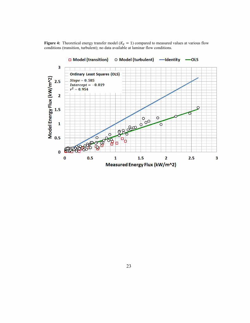
Figure 4: Theoretical energy transfer model (� = 1) compared to measured values

at various flow conditions (transition, turbulent); no data available at laminar flow

conditions. ................................................................................................................... 23

Figure 5: Optimized energy transfer model (�) compared to measured values at

various flow conditions (transition, turbulent); no data available at laminar flow

conditions. ................................................................................................................... 24

Figure 6: An overview of MD simulation (Haile, 1992). ......................................... 27

Figure 7: Basic steps, software, and databases used to perform MD simulations. ... 33

Figure 8: Using MD simulation to estimate liquid evaporation rates. ...................... 43

Figure 9: Illustration of a typical starting configuration for an MD simulation used to

estimate self and mutual diffusion coefficients. ......................................................... 45

Figure 10: Single particle mean square displacement (MSD) for various gasses at

atmospheric pressure; time delay of 0.2 ns to 1.8 ns was used to estimate the slope of

MSD vs time delay...................................................................................................... 47

Figure 11: Collective mean square displacement (MSD) for “tagged” equimolar

binary gas mixtures at atmospheric pressure; time delay of 0.5 ns to 1.5 ns was used to

estimate the slope of MSD vs time delay. ................................................................... 48

Figure 12: Bar chart; self-diffusion coefficients for various gases at atmospheric

pressure; estimates from single particle and collective MSD are compared with

Chapman-Enskog. ....................................................................................................... 49

x

Figure 13: Scatter chart; self-diffusion coefficients for various gases at atmospheric

pressure; estimates from single particle and collective MSD are compared with

Chapman-Enskog. ....................................................................................................... 50

Figure 14: Collective mean square displacement (MSD) for equimolar binary gas

mixtures at atmospheric pressure; time delay of 0.6 ns to 1.6 ns was used to estimate

the slope of MSD vs time delay. ................................................................................. 52

Figure 15: Bar chart; binary gas diffusion coefficients at atmospheric pressure;

Molecular Dynamics (MD) vs Chapman-Enskog (CE) Theory. ................................ 53

Figure 16: Scatter chart; binary gas diffusion coefficients at atmospheric pressure;

Molecular Dynamics (MD) vs Chapman-Enskog (CE) Theory. ................................ 54

Figure 17: Illustration of a typical starting configuration for an MD simulation used

to estimate relative solvent drying times of liquids in Air. ......................................... 57

Figure 18: Bar chart; relative solvent drying times at 296 K and 1 atm; MD simulation

estimates are compared with experimentally measured values. ................................. 60

Figure 19: Scatter chart; relative solvent drying times at 296 K and 1 atm; MD

simulation estimates are compared with experimentally measured values ................ 61

Figure J - 1: Spread of DIETHYL ETHER as it evaporates into Air at 296 K and 1

atm; rate of spread can be estimated from the slope of the least-squares line. ........... 92

Figure J - 2: Spread of ACETONE as it evaporates into Air at 296 K and 1 atm; rate

of spread can be estimated from the slope of the least-squares line. .......................... 93

Figure J - 3: Spread of ETHANOL as it evaporates into Air at 296 K and 1 atm; rate


Figure J - 4: Spread of METHANOL as it evaporates into Air at 296 K and 1 atm;

rate of spread can be estimated from the slope of the least-squares line. ................... 95

Figure J - 5: Spread of BENZENE as it evaporates into Air at 296 K and 1 atm; rate


Figure J - 6: Spread of CYCLOHEXANE as it evaporates into Air at 296 K and 1

atm; rate of spread can be estimated from the slope of the least-squares line. ........... 97

xi

Figure J - 7: Spread of N-PENTANE as it evaporates into Air at 296 K and 1 atm;

rate of spread can be estimated from the slope of the least-squares line. ................... 98

Figure J - 8: Spread of 2-PENTANONE as it evaporates into Air at 296 K and 1 atm;

rate fo spread can be estimated from the slope of the least-squares line. ................... 99

1

Chapter 1: Introduction

Today, whether it be an industrial, commercial, or consumer setting, the use of

chemical substances in the liquid state is common practice. These liquid chemicals can

be used as reactants, cleaning solvents, coatings, fuels, and additives (Smith, 2001).

Liquid chemicals can evaporate and become airborne, which may result in human

exposure. Acute (short-term) and chronic (long-term) exposures to hazardous

substances may lead to adverse health effects (cancer, non-cancer). Since it is not

always possible to measure airborne contaminant concentrations for all relevant

exposure scenarios, validated models can be of great help to exposure assessors.

Models based on mass balance principles are commonly used to estimate

chemical concentrations in air (Reinke, 1997; Fehrenbacher, et al., 1996; Keil, 2003;

Jayjock, et al., 2011). The risk assessment community and certain regulatory agencies

routinely make use of such models to assess potential human exposures to volatile

liquid substances. In order to estimate these airborne concentrations, one must also

have a means of estimating liquid evaporation rates, which are a necessary input for

exposure models.

Various models have been developed for estimating evaporation rates (Smith,

2001; Arnold, et al., 2001; Barry, 1995; Braun, et al., 1989; Gajjar, et al., 2013;

Hummel, et al., 1996; Mackay, et al., 1973; Nielsen, et al., 1995; Okamoto, et al., 2010;

Olsen, et al., 1995). These models are generally used for pure liquids and do not take

2

evaporative cooling into account, which can overestimate evaporation rates. Some

models address evaporation of binary mixtures but assume isothermal conditions

(Okamoto, et al., 2010; Olsen, et al., 1995).

One of the objectives of this thesis is to develop an evaporation model that can

take evaporative cooling into account, and estimate steady-state evaporation rates for

pure liquids as well as liquid mixtures for various flow conditions (laminar, transition,

turbulent). The developed model is referred to as the Simultaneous Mass and Energy

Evaporation (SM2E) model (Choudhary, 2016). It is based on theoretical expressions

for mass and energy transfer, which were refined to optimize agreement with

experimental measurements.

Evaporation models generally require input parameters such as vapor pressures,

diffusion coefficients, heats of vaporization, and activity coefficients. In some cases,

it is possible to find estimates for these parameters from published sources (e.g.,

publications, property handbooks). However, no such parameters will be available for

“new substances” that have not yet been synthesized or introduced into commerce. In

such instances, it may be possible to use molecular dynamics (MD) simulation to

estimate the required input parameters. It may also be possible to estimate evaporation

rates directly from MD simulation.

MD simulations were first conducted in the 1950s (Haile, 1992). These

methods are becoming more prevalent due to ongoing computational enhancements

and members of the research community are turning to these methods with new

3

questions and problems. Given a set of initial conditions, MD simulations can be used

to compute the movement of individual molecules under the action of forces. If it is

possible to simulate motion at the molecular level, then it should be possible to use MD

simulation to study molecular diffusion in gases and the evaporation of liquids in air.

But if MD simulation is used to estimate diffusion coefficients and relative solvent

drying times, how will these estimates compare to results from other theories or

experiments?

Various MD simulations have been conducted to study liquid evaporation and

diffusion. MD simulation has been used to study the evaporation of liquid argon

droplets into argon vapor (Long, et al., 1996) and also liquid xenon droplets into

nitrogen gas (Consolini, et al., 2003). The evaporation of a thin layer of liquid water

into vacuum was investigated using the TIP4P water model with periodic boundary

conditions (PBCs) applied in all Cartesian directions (Yang, et al., 2005). More

recently, the evaporation and condensation of thin liquid argon films sandwiched

between two solid walls in the Cartesian direction with PBCs applied in the � and �

Cartesian directions was also studied (Yu, et al., 2012).

MD simulation has been used to study the diffusion of nitric oxide in liquid

water (Zhou, et al., 2005) and also diffusion of hydrogen, carbon monoxide, and water

in liquid n-alkanes at elevated temperatures and pressures (Makrodimitri, et al., 2011),

where n-alkanes were modeled based on the united-atom Transferable Potentials for

Phase Equilibria (TraPPE-UA) and simulation runs were on the order of 30

4

nanoseconds (ns). Mutual diffusion coefficients for gas mixtures of ethane/nitrogen

and n-pentane/nitrogen have been estimated using MD simulation and compared to

measured values (Chae, et al., 2011). MD simulation has also been used to study

diffusion coefficients of heptane isomers in nitrogen in the range of 500 to 1000 K

(Chae, et al., 2011), where results were compared to estimates from Chapman-Enskog

(CE) theory and the all-atom Optimized Potentials for Liquid Simulations (OPLS-AA)

was used to describe molecular interactions and simulation runs were on the order of

14 ns.

Another objective of this thesis is to use MD simulation to estimate gas phase

self and mutual diffusion coefficients using single-particle and collective mean-square

displacement (MSD) methods and compare these results to estimates from CE theory.

MD simulations will also be used to study the evaporation of liquid solvents into air

and relative drying times will be compared with measured values.

5

Chapter 2: Simultaneous Mass and Energy Evaporation (SM2E) Model

In this chapter, the Simultaneous Mass and Energy Evaporation (SM2E) model

is presented. The SM2E model is based on theoretical models for mass and energy

transfer. When compared to measured evaporation rates, the theoretical models

systematically under or over predicted at various flow conditions: laminar, transition,

turbulent. These models were harmonized with experimental measurements to

eliminate systematic under or over predictions; a total of 113 measured evaporation

rates were used. The SM2E model can be used to estimate evaporation rates for pure

liquids as well as liquid mixtures at laminar, transition, and turbulent flow conditions.

However, due to limited availability of evaporation data, the model has so far only been

tested against data for pure liquids and binary mixtures. The model can take

evaporative cooling into account and when the temperature of the evaporating liquid or

liquid mixture is known (e.g., isothermal evaporation), the SM2E model reduces to a

mass transfer-only model.

2.1 Model Development and Input Parameters

The steady-state evaporation of a liquid is illustrated in Figure 1. In this

scenario, the air flow over the evaporating liquid is one-dimensional and it is assumed

that convection in the direction is faster than diffusion in the direction. The velocity

profile in the boundary layer is estimated by Equation (1) (Middleman, 1998), where

6

��(�) is the air velocity in the boundary layer in the direction as a function of �, ��

is the air velocity outside the boundary layer in the direction, � is the Cartesian

coordinate, and � is the boundary layer thickness. The mean velocity in the boundary

layer �� is given by Equation (2) and it is used to represent the velocity in the boundary

layer.

−=2

2)(

δδzz

Uzv bulkx (1)

bulkbulk

x

m UU

dz

dzzv

v 67.03

2)(

0

0 ≈==

∫

∫δ

δ

(2)

7

Figure 1: Steady-state evaporation of a liquid into a flowing stream of air; the presence of a boundary

layer is assumed at the liquid-to-air interface; a no-slip condition is applied at � = 0; the velocity

profile in the boundary layer is parabolic; bottom-side energy transfer is also possible.

The mass transport equation and relevant boundary conditions are given by

Equations (3) and (4), where �� is the molar concentration of chemical �, ��∗ is the

molar concentration of chemical � at liquid-to-air interface, �� is the molar

concentration of chemical � far from the liquid-to-air interface, and �� ! is the gas-

phase binary diffusion coefficient of chemical � in air.

8

2

2

z

CD

x

Cv i

airii

m ∂∂=

∂∂

− (3)

∞→=

==

==

∞

∞

zCC

zCC

xCC

ii

ii

ii

at

0at

0at

* (4)

Evaporation produces an outward directed flow of vapor (blowing), which

impedes heat transfer to the evaporating liquid and can thus reduce mass transfer

compared to mass transfer by just diffusion (absence of blowing) (Middleman, 1998).

The mass flux for pure and liquid mixtures with a blowing correction factor ("�#) is

given by Equation (5), where $�∗ is the partial pressure of chemical � at liquid-to-air

interface, $�� is the partial pressure of chemical � far from the liquid-to-air interface,

$�% & is the vapor pressure of chemical �, $'(' � is the total pressure, ) is the gas

constant, *��+��, is the steady-state temperature of evaporating liquid, � is the mole

fraction of chemical � in the liquid mixture, �� is the mole fraction of chemical � far

from the liquid-to-air interface, -� is the steady-state mass flux of chemical �, �.� is

the molecular weight of chemical �, �/ is the mass flux correction factor, 01 is the gas-

phase mass transfer coefficient, 2 is the length of the evaporating liquid, 3� activity

9

coefficient of chemical � in the liquid mixture, and )4 is a symbol used in the blowing

correction factor, [ ]

A

A

R

RBCF

+= 1ln.

[ ]i

A

A

liquid

ii

vap

iimairiM

i

liquid

iigM

iiigMi

z

iairiMi

MWR

R

TR

PPx

L

vDK

MWBCFRT

PPkK

MWBCFCCkKMWBCFz

CDKn

+

−

=

−=

−=∂

∂−=

∞−

∞

∞

=−

1ln4

)(

5.0

*

*

0

γπ

(5)

−

−=

∞

total

i

vap

ii

i

total

i

vap

ii

A

P

Px

xP

Px

Rγ

γ

1

(6)

The energy transport equation, relevant boundary conditions, and energy flux

are given by Equations (7), (8), and (9), respectively, where 0 �! is the thermal

conductivity of air, �5 is the energy flux correction factor, 6 is the steady-state energy

flux due to evaporation, ℎ1 is the gas-phase heat transfer coefficient, * is the air

temperature, *� is the air temperature far from the liquid-to-air interface, and 8 �! is

the thermal diffusivity of air.

10

2

2

z

T

x

Tv airm ∂

∂=∂∂ α (7)

∞→=

====

∞

∞

zTT

zTT

xTT

Liquid

at

0at

0at

(8)

)(4

)(

5.0

0

∞∞

=

−

=−=

∂∂−= TT

L

vkKTThK

z

TkKq liquid

air

mairEliquidgE

z

airE απ (9)

The SM2E model is given by Equation (10), where ∆:�% & is the heat of

vaporization of chemical �, -� and 6 are obtained from Equations (5) and (9),

respectively, and � is the number of chemical substances evaporating, which will be

one for a pure liquid. When applicable, the term 6(';<! can be used to account for

additional routes of energy transfer.

∑=

+=∆N

i

other

i

vap

ii qqMW

Hn

1

(10)

In this thesis, gas-phase binary diffusion coefficients in air were estimated using

Equation (11) (Hummel, et al., 1996), where * %1 is the arithmetic mean of *��+��, and

*�. Relative to experimental measurements of binary diffusion coefficients in air

11

(Cussler, 2009), the error in Equation (11) could approximately be ± 18%. The thermal

conductivity and thermal diffusivity of air were estimated using Equations (12) and

(13), respectively (The Engineering ToolBox, 2014); these equations are valid from -

238 oF to 752 oF or (123 K to 673 K). The vapor pressure $�% & of relevant substances

was estimated using Equation (14), the Antoine equation. Please refer to Table 2 for

relevant Antoine coefficients and heats of vaporization.

[ ]

760

)(

1

29

1)(9-E09.4

.0

5.0

9.1

2

mmHgP

mol

gMW

mol

gMW

KT

s

mD

total

i

i

avg

airi

−

−

+

∗

=

(11

)

3-E3925)(*5-E9526 .KT.Km

Wk avgair +=

− (12)

[ ] 6-E722.6)(*8-E585.5)(*10-E363.12

2

−+=

KTKT

s

mavgavgairα (13)

+−−

= CKT

BA

vap

i

liquidmmHgP15.273)(

10)barsor ( (14)

12

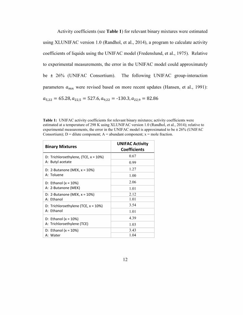
Activity coefficients (see Table 1) for relevant binary mixtures were estimated

using XLUNIFAC version 1.0 (Randhol, et al., 2014), a program to calculate activity

coefficients of liquids using the UNIFAC model (Fredenslund, et al., 1975). Relative

to experimental measurements, the error in the UNIFAC model could approximately

be ± 26% (UNIFAC Consortium). The following UNIFAC group-interaction

parameters =�> were revised based on more recent updates (Hansen, et al., 1991):

=?,AA = 65.28, =AA,? = 527.6, =G,AA = -130.3, =AA,G = 82.86

Table 1: UNIFAC activity coefficients for relevant binary mixtures; activity coefficients were

estimated at a temperature of 298 K using XLUNIFAC version 1.0 (Randhol, et al., 2014); relative to

experimental measurements, the error in the UNIFAC model is approximated to be ± 26% (UNIFAC

Consortium); D = dilute component; A = abundant component; x = mole fraction.

Binary Mixtures UNIFAC Activity

Coefficients

D: Trichloroethylene, (TCE, x = 10%) A: Butyl acetate

0.67

0.99

D: 2-Butanone (MEK, x = 10%) A: Toluene

1.27

1.00

D: Ethanol (x = 10%) A: 2-Butanone (MEK)

2.06

1.01

D: 2-Butanone (MEK, x = 10%) A: Ethanol

2.12

1.01

D: Trichloroethylene (TCE, x = 10%) A: Ethanol

3.54

1.01

D: Ethanol (x = 10%) A: Trichloroethylene (TCE)

4.39

1.03

D: Ethanol (x = 10%) A: Water

3.43

1.04

13

Table 2: Antoine equation coefficients for relevant substances (Knovel, 2013; Poling, et al., 2001);

data for Heat of Vaporization (NIST, 2014; Poling, et al., 2001; Smith, et al., 2005); for Xylene, used

property values for m-Xylene since commercial Xylene can contain up to 65% m-Xylene (U.S. EPA,

2014) and m-Xylene, o-Xylene, p-Xylene have similar vapor pressures and heats of vaporization.

Substance A B C

Temperature

Range

(Celsius)

Heat of

Vaporization

(kJ/mol)

Methanol 8.09126 1582.91 239.096 -98 to 239 37.6

N-propanol 7.77374 1518.16 213.076 -73 to 264 47

1-pentanol 7.21775 1333.96 169.781 -27 to 315 57

Acetone 7.31414 1315.67 240.479 -95 to 235 31.3

Methyl ethyl ketone 7.20103 1325.15 227.093 -85 to 262 34

2-octanone 7.08024 1475.8 178.43 -20 to 351 50.6

Hexane 6.9895 1216.92 227.451 -95 to 234 31

N-heptane 7.04605 1341.89 223.733 -91 to 267 36

Octane 7.14462 1498.96 225.874 -57 to 296 41

Benzene 6.81404 1090.43 197.146 -40 to 289 33.9

Toluene 7.1362 1457.29 231.827 -95 to 319 37

Xylene 7.18115 1573.02 226.671 -48 to 344 41

1-hexanol 7.3423 1538.76 187.498 -45 to 338 61

1-heptanol 7.18822 1482.06 167.773 -34 to 359 67

2-octanol 6.99299 1420.06 165.53 -32 to 364 67.9

Water 8.05573 1723.64 233.076 0 to 374 40.63

Butyl acetate 7.2341 1515.76 222.077 -74 to 307 43

Ethanol 8.13484 1662.48 238.131 -114 to 243 42.3

Trichloroethylene 6.87981 1157.83 202.58 -74 to 298 34.5

Cyclohexane1 3.93002 1182.774 220.618 9 to 105 29.97

Diethyl Ether1 4.10962 1090.640 231.200 -43 to 55 26.52

n-Pentane1 3.97786 1064.840 232.014 -44 to 58 25.79

2-Pentanone1 4.15140 1316.730 215.380 10 to 127 33.44

1 Antoine coefficients for these substances give vapor pressure is in bars, all others give vapor

pressure in mmHg.

14

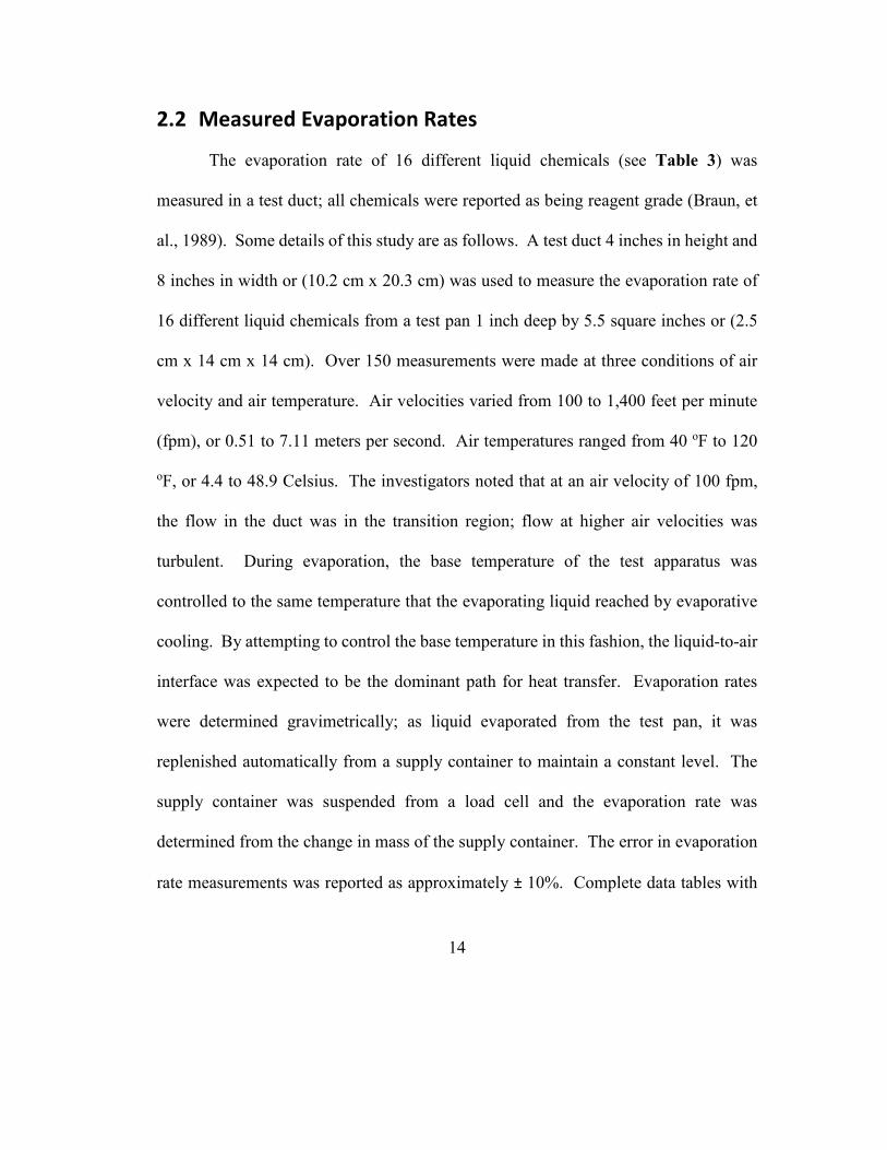
2.2 Measured Evaporation Rates

The evaporation rate of 16 different liquid chemicals (see Table 3) was

measured in a test duct; all chemicals were reported as being reagent grade (Braun, et

al., 1989). Some details of this study are as follows. A test duct 4 inches in height and

8 inches in width or (10.2 cm x 20.3 cm) was used to measure the evaporation rate of

16 different liquid chemicals from a test pan 1 inch deep by 5.5 square inches or (2.5

cm x 14 cm x 14 cm). Over 150 measurements were made at three conditions of air

velocity and air temperature. Air velocities varied from 100 to 1,400 feet per minute

(fpm), or 0.51 to 7.11 meters per second. Air temperatures ranged from 40 oF to 120

oF, or 4.4 to 48.9 Celsius. The investigators noted that at an air velocity of 100 fpm,

the flow in the duct was in the transition region; flow at higher air velocities was

turbulent. During evaporation, the base temperature of the test apparatus was

controlled to the same temperature that the evaporating liquid reached by evaporative

cooling. By attempting to control the base temperature in this fashion, the liquid-to-air

interface was expected to be the dominant path for heat transfer. Evaporation rates

were determined gravimetrically; as liquid evaporated from the test pan, it was

replenished automatically from a supply container to maintain a constant level. The

supply container was suspended from a load cell and the evaporation rate was

determined from the change in mass of the supply container. The error in evaporation

rate measurements was reported as approximately ± 10%. Complete data tables with

15

measured evaporation rates are included in Appendix A of the study (Braun, et al.,

1989).

Table 3: Evaporation rates were measured for 16 different liquid chemicals in a test duct; all

chemicals were reported as being reagent grade; evaporation rates were measured gravimetrically

(Braun, et al., 1989).

Aliphatic

Compounds

Aromatic

Compounds Alcohols Ketones Other

Heptane Benzene Methanol 1-Hexanol Methyl Ethyl

Ketone

Water

Octane Toluene n-Propanol 1-Heptanol 2-Octanone

Hexane Xylene n-Pentanol 2-Octanol Acetone

In another study (Olsen, et al., 1995), evaporation rates were measured at a

lower air velocity (33 fpm or 0.17 meters per second) while the liquid temperature was

actively controlled to approximately 73 oF (or 22.8 Celsius). Evaporation rates were

reported for pure liquids and also for binary mixtures (see Table 4); all chemicals were

reported as being of high purity (greater than 99.5% by weight). Some details of this

study are as follows. A test duct having a square section (0.100 m x 0.100 m) and an

evaporation surface length of 0.075 m was used to measure the evaporation rate of pure

liquid chemicals and 7 binary liquid mixtures. During evaporation, the temperature of

the evaporating liquid was thermostatically controlled to simulate isothermal

evaporation. Evaporation rates were determined from the concentration of the

evaporating liquid in the effluent air and the total air flow rate; concentrations were

measured using an infrared (IR) photo-acoustic detector (Multi-gas Monitor Type

16

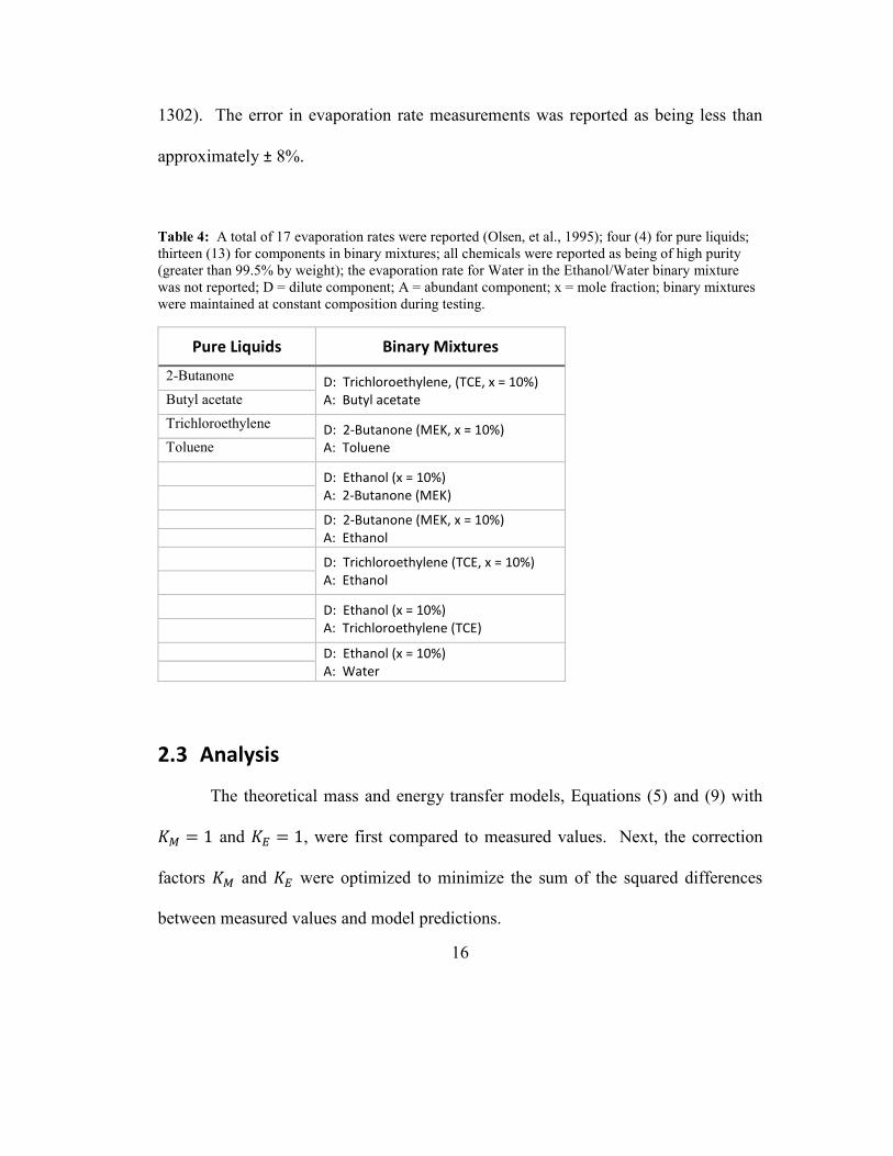
1302). The error in evaporation rate measurements was reported as being less than

approximately ± 8%.

Table 4: A total of 17 evaporation rates were reported (Olsen, et al., 1995); four (4) for pure liquids;

thirteen (13) for components in binary mixtures; all chemicals were reported as being of high purity

(greater than 99.5% by weight); the evaporation rate for Water in the Ethanol/Water binary mixture

was not reported; D = dilute component; A = abundant component; x = mole fraction; binary mixtures

were maintained at constant composition during testing.

Pure Liquids Binary Mixtures

2-Butanone D: Trichloroethylene, (TCE, x = 10%) A: Butyl acetate Butyl acetate

Trichloroethylene D: 2-Butanone (MEK, x = 10%) A: Toluene Toluene

D: Ethanol (x = 10%) A: 2-Butanone (MEK)

D: 2-Butanone (MEK, x = 10%) A: Ethanol

D: Trichloroethylene (TCE, x = 10%) A: Ethanol

D: Ethanol (x = 10%) A: Trichloroethylene (TCE)

D: Ethanol (x = 10%) A: Water

2.3 Analysis

The theoretical mass and energy transfer models, Equations (5) and (9) with

�/ = 1 and �5 = 1, were first compared to measured values. Next, the correction

factors �/ and �5 were optimized to minimize the sum of the squared differences

between measured values and model predictions.

17

Experiments at Transition and Turbulent Flow Conditions

For the evaporation rates measured at transition and turbulent flow conditions,

a total of 157 measured evaporation rates were reported (Braun, et al., 1989). Of these

reported values, the investigators indicated that a total of six measured values did not

meet equilibrium requirements since the measured liquid temperature was higher than

the air temperature. These six values were not included in this analysis.

Also, the base temperature of the test apparatus was controlled to the same

temperature that the evaporating liquid reached by evaporative cooling. By attempting

to control the base temperature in this fashion, the liquid-to-air interface was expected

to be the dominant path for heat transfer. However, this control was not ideal in all

instances. The absolute difference in liquid and base temperatures ranged from 0 to 17

oF. Other than its dimensions, not much else is known about the test pan. To ensure

that the liquid-to-air interface was the dominant path for heat transfer, in this analysis,

only those measured values were used for which the absolute difference in liquid and

base temperature was less than 2 oF. In addition, since temperatures were measured to

a tolerance of ±1 oF, only those values were used for which the absolute difference

between liquid and air temperature was greater than 2 oF.

Based on these data exclusions, the total number of measured values available

for model refinements was 96 compared to the original 157; 28 of these 96 values were

at an air velocity of 100 fpm (transition flow), while 68 were at air velocities ranging

18

from 500 to 1,400 fpm (turbulent flow). In the original set of 157 measurements, 43

values were at an air velocity of 100 fpm (transition flow), while 114 were at air

velocities ranging from 500 to 1,400 fpm (turbulent flow).

Experiments at Laminar Flow Conditions

For the evaporation rates measured at laminar flow conditions, a total of 17

measured evaporation rates were reported (Olsen, et al., 1995). Since the temperature

of the evaporating liquid was actively controlled in these experiments, the available

data did not permit estimation of the correction factor �5 for laminar flow conditions.

However, the ratio JKJL for the transition and turbulent flow conditions was

approximately 0.60. The correction factor �5 for laminar flow conditions was

estimated based on the average of this ratio at transition and turbulent flow conditions.

2.4 Results and Discussion

The theoretical and optimized mass transfer models are compared with

measured values in Figure 2 and Figure 3, respectively. The theoretical and optimized

energy transfer models are compared with measured values in Figure 4 and Figure 5,

respectively. Optimized values for the model correction factors at different air flow

conditions are presented in Table 5. Based on these results, it is evident that different

19

air flows (laminar, transition, turbulent) affect mass and energy transfer. However, this

impact is well within an order of magnitude.

The theoretical mass transfer model seems most appropriate for turbulent flow,

while it systematically under and over estimates at transition and laminar flows,

respectively. The theoretical energy transfer model is expected to overestimate at

laminar flows while it underestimates at transition and turbulent flows. The optimized

transfer models eliminate these systematic under and over predictions. For transition

and turbulent flows, the correction factor for energy transfer �5 is approximately 60%

greater than the correction factor for mass transfer �/. Transfer coefficients can

increase in the transition region due to fast intermixing (Sawhney, 2010); this is

supported by the optimized values in Table 5.

The goal of this assessment was to start with theoretical expressions for mass

and energy transfer and develop the SM2E model. The SM2E model is applicable to

laminar, transition, and turbulent flow conditions. When the temperature of the

evaporating liquid or liquid mixture is known (e.g., isothermal evaporation), the SM2E

model reduces to a mass transfer-only model.

Additional experiments can be performed to further refine the SM2E model.

For example, there is a significant need for obtaining and publishing evaporation rates

for multi-component mixtures so that models can be validated against a robust data set.

Further, the air speed used for laminar conditions (0.17 meters per second) is likely an

order of magnitude higher compared to a typical indoor residential environment.

20

Measuring evaporation rates at lower air speeds (0.01 – 0.02 meters per second) will

help to clarify how well the SM2E model performs for indoor residential settings.

Table 5: Optimized model correction factors at different air flow conditions.

Model Correction

Factor

Air Flow Condition

Laminar Transition Turbulent

MK 0.4572 1.7497 0.9859

EK 0.7417 2.7920 1.6264

21

Figure 2: Theoretical mass transfer model (�/ = 1) compared to measured values at various flow

conditions (laminar, transition, turbulent).

22

Figure 3: Optimized mass transfer model (�/) compared to measured values at various flow

conditions (laminar, transition, turbulent).

23

Figure 4: Theoretical energy transfer model (�5 = 1) compared to measured values at various flow

conditions (transition, turbulent); no data available at laminar flow conditions.

24

Figure 5: Optimized energy transfer model (�5) compared to measured values at various flow

conditions (transition, turbulent); no data available at laminar flow conditions.

25

2.5 Conclusions

Based on evaporation experiments reported in the literature, the Simultaneous

Mass and Energy Evaporation (SM2E) model was developed. This model was based

on theoretical models for mass and energy transfer. These theoretical models were

harmonized with experimental measurements at various flow conditions (laminar,

transition, turbulent). The SM2E model can be used to estimate evaporation rates for

pure liquids as well as liquid mixtures at laminar, transition, and turbulent flow

conditions. However, due to limited availability of evaporation data, the model has so

far only been tested against data for pure liquids and binary mixtures. The model can

take evaporative cooling into account and when the temperature of the evaporating

liquid or liquid mixture is known (e.g., isothermal evaporation), the SM2E model

reduces to a mass transfer-only model.

26

Chapter 3: Estimating Transport Properties Using MD Simulation

MD simulation is comprised of developing molecular models and simulating

those models (see Figure 6). An MD simulation determines molecular trajectories by

numerically solving Newton’s equations of motion for a system of interacting

molecules, where forces between molecules are calculated using a particular form for

molecular interactions. These molecular trajectories can then be analyzed to estimate

dynamic properties like diffusion coefficients and relative solvent drying times. In this

thesis, simulations are conducted using the NAMD MD simulation package (Phillips,

et al., 2005). Also, the Transferrable Potentials for Phase Equilibria (TraPPE) (The

Siepmann Group, 2015) are used for all chemicals listed in Table 6, except water, for

which the TIP3P potential is used (Jorgensen, et al., 1983).

Table 6: Coordinate files for these chemicals were obtained from ChemSpider.

2-Pentanone Benzene Diethyl Ether Methanol Propane

n-Pentane Carbon Dioxide Ethanol Nitrogen Water

Acetone Cyclohexane Methane Oxygen

27

Figure 6: An overview of MD simulation (Haile, 1992).

3.1 Equations of Motion

MD simulations are based on Newton’s second law. The force exerted on a

molecule � is given by Equation (15), where #� is the force, M� is the mass, =� is the

acceleration, and N� is the position:

#� = M�=� = M� OAN�OPA (15)

The force exerted on a molecule � can also be expressed as the negative gradient

of the potential energy Q of the system:

Molecular Dynamics (MD) Simulation

Develop Molecular Models

Molecular Interactions

Equations of Motion

Simulate Molecular Models

Generate Trajectories

Analyze Trajectories

28

#� = −S�Q = − OQON� (16)

Equations (15) and (16) can be combined to yield:

− OQON� = M� OAN�OPA (17)

Given a functional form for the potential energy, and initial positions and

velocities for the molecules of the system, Equation (17) can be used to describe the

positions, velocities, and accelerations of the molecules as they vary with time.

3.2 Molecular Interactions

The intra- and intermolecular forces within a system are often represented as

a summation of bonded and nonbonded interactions as shown in Equation (18).

Q(NT) = U Q�(>,<,(NT) + U Q>(>�(>,<,(NT) (18)

29

3.2.1 Bonded Interactions

Bonded interactions include terms for bond stretching (bonds), angle bending

(angles), and bond rotations and out-of-plane bending (dihedrals) (Leach, 2001; The

Siepmann Group, 2015):

U Q�(>,<,(NT) = Q�(>,W + Q >1�<W + Q,�;<,! �W (19)

The first term in Equation (19) models interactions between pairs of bonded

atoms and is represented using a Hooke’s law formulation as shown in Equation (20),

where ��(>, is the bond constant, N�X is the distance between the bonded atoms, and NY

is the reference bond length (Leach, 2001; The Siepmann Group, 2015):

Q�(>,W = U ��(>,ZN�X − NY[A�(>,W

(20)

The second term in Equation (19) accounts for the deviation of angles from

their reference values (Leach, 2001; The Siepmann Group, 2015). This is also

represented using a Hooke’s law formulation as shown in Equation (21), where �\ is

the angle constant, ] is the bond angle between atoms A-B-C and is defined as the

angle between the bonds A-B and B-C, and ]Y is the reference bond angle:

30

Q >1�<W = U �\(] − ]Y)A

>1�<W

(21)

The third term in Equation (19) models bond rotations and out-of-plane bending

as measured by the angle (dihedral angle) between the planes formed by four

consecutively bonded atoms A-B-C-D, where one plane is defined by A-B-C and the

second by B-C-D (Leach, 2001; The Siepmann Group, 2015). These types of potentials

are represented as a cosine series as shown in Equation (22), where - + 1 is the number

of terms in the cosine series, �> are constants, ^ is the dihedral angle as described

earlier, and _ is the phase shift angle.

Q,�;<,! �W = U U �>`1 + abc(-^ − _)d>

>eY,�;<,! �W

(22)

3.2.2 Nonbonded Molecular Interactions

Nonbonded interactions include terms for van der Waals and electrostatic

interactions. These interactions are calculated for pairs of atoms (�, f) that are separated

by at least - bonds. Such pairs of atoms (�, f) are said to have a 1, - + 1 relationship.

U Q>(>�(>,<,(NT) = Q% > ,<! h �W + Q<�<i'!(W' '�i (23)

31

The first term in Equation (23) accounts for van der Waals interactions (Leach,

2001; The Siepmann Group, 2015). It is represented by the Lennard-Jones (LJ) 12-6

potential given by Equation (24), where N�X is the distance between atom pairs (�, f), -j�X is the minimum potential value, and )��> is the distance at which the potential

reaches its minimum value:

Q% > ,<! h �W = U U k�X lm)��>N�X noA − 2 m)��>N�X npqr

Xe�so

r

�eo

(24)

The second term in Equation (23) accounts for electrostatic interactions and is

represented by Coulomb’s law as shown in Equation (25), where N�X is the distance

between atom pairs (�, f), jY is the permittivity of free space, and 6� is the charge on

atom �, and 6X is the charge on atoms f (Leach, 2001; The Siepmann Group, 2015):

Q<�<i'!(W' '�i = U U 6�6X4ujYN�Xr

Xe�so

r

�eo

(25)

32

3.3 Generate Trajectories

To generate trajectories for molecules in an MD simulation, the equations of

motion mentioned in Chapter 3.1 are solved using a finite difference method. These

finite difference methods approximate positions and velocities as Taylor series

expansions (Leach, 2001). The method used to calculate molecule positions and

velocities in NAMD is the velocity Verlet method. Given initial molecule positions

and velocities at a time P, the position at some later time P + �P is given by:

N(P + �P) = N(P) + �P�(P) + 12 �PA=(P) (26)

With an estimate for the position N(P + �P), the acceleration =(P + �P) can be

derived from the interaction potential given by Equation (18), and then the velocity at

some time P + �P is given by:

�(P + �P) = �(P) + 12 �PA`=(P) + =(P + �P)d (27)

33

3.4 Simulation Methodology

In order to prepare, run, and analyze the results of an MD simulation, various

software and databases need to be referenced. The basic steps, software, and databases

used to perform MD simulations in this work are summarized in Figure 7.

Figure 7: Basic steps, software, and databases used to perform MD simulations.

3.4.1 Obtain Coordinate File

In order to compute the movement of individual molecules under the action of

forces, it is important to be able to identify the atoms in a particular molecule and their

locations in three-dimensional (3D) space. Coordinate files contain just this type of

information and are available in many formats. In this work, coordinate files are

obtained from ChemSpider (Royal Society of Chemistry, 2015), an online chemical

structure database (CSD). The files obtained from ChemSpider use the MDL Molfile

Obtain coordinate file

• ChemSpider

Convert coordinate file to desired format

• Open Babel

Define initial configuration

• PACKMOL

Prepare structure and coordinate files

• VMD

Generate trajectories

• NAMD

Analyze trajectories

• VMD

• Microsoft Excel

34

format, which can be identified by the .mol file name extension. Coordinate files were

obtained for the chemicals listed in Table 6. An example coordinate file can be found

in Appendix A: Example MDL Molfile Coordinate File (Methane).

3.4.2 Convert Coordinate File to Desired Format

The coordinate files obtained from ChemSpider are in MDL Molfile format.

However, for the MD simulation package used in this work (NAMD), the Protein Data

Bank (PDB) format is needed. The PDB file format can be identified by the .pdb file

name extension. Chemical file formats were converted from MDL Molfile to PDB

using Open Babel (O'Boyle, et al., 2011), a chemical toolbox that can read, write, and

convert many different chemical file formats. An example coordinate file can be found

in Appendix B: Example PDB Coordinate File (Methane).

3.4.3 Define Initial Configuration

It is important to realize that the coordinate files available thus far only list the

atoms and their locations for a particular molecule. However, this work will perform

MD simulations for systems that contain many number of molecules in various

configurations. So the next step is to define an initial configuration for MD simulation.

This is done using PACKMOL (Martinez, et al., 2009), which creates initial

configurations (in PDB format) by packing molecules in defined regions of space.

Users need only provide coordinate files for each type of molecule, the number of

molecules of each type, and the spatial constraints that each type of molecule must

35

satisfy. Example PACKMOL input files used to prepare initial configurations for this

work can be found in Appendix C: Example PACKMOL Configuration Files.

3.4.4 Prepare Structure and Coordinate Files

Now that an initial configuration PDB file has been prepared using PACKMOL,

the next step is to prepare a final PDB configuration file and also a Protein Structure

File (PSF). Whereas NAMD obtains coordinates from the PDB configuration file,

structural information such as bonding is obtained from the PSF file.

Before the PDB configuration file can be finalized and a PSF file created, a

force field topology file is needed. This file contains information regarding atom types,

charges, and how atoms in a molecule are connected. The topology file used for this

work can be found in Appendix D: NAMD Topology File.

Once a topology file is available, Visual Molecular Dynamics (VMD)

(Humphrey, et al., 1996), a molecular visualization program, is used to prepare a PSF

file and also finalize the PDB configuration file. An example VMD script file used to

prepare PSF files and finalize PDB configuration files for this work can be found in

Appendix E: Example VMD Script File Used to Prepare PSF and Final PDB.

What does it mean to finalize the PDB file? For example, a Methane molecule

is comprised of one Carbon atom bonded to four Hydrogen atoms. The Methane PDB

file (see Table B - 1) was used to prepare an initial configuration using PACKMOL

(see Table C - 1). For this work, molecular interactions (see Chapter 3.2) are modeled

36

using the Transferrable Potentials for Phase Equilibria (TraPPE) for all chemicals listed

in Table 6, except Water, for which the TIP3P potential is used. The TraPPE potential

used for Methane does not model the Hydrogen atoms explicitly, but rather it models

Methane as a pseudo CH4 atom. Thus, the initial configuration file is finalized by

removing the Hydrogen atoms from the Methane molecules (see Table E - 1).

3.4.5 Generate Trajectories

Running an MD simulation using NAMD requires a PDB configuration file,

PSF file, force field parameter file, and a configuration file. The PDB configuration

and PSF files were described previously and are obtained using VMD (see Chapter

3.4.4).

The parameter file contains the inputs needed to describe the bonded and

nonbonded interactions described in Chapter 3.2. As indicated previously, for this

work, the Transferrable Potentials for Phase Equilibria (TraPPE) are used for all

chemicals listed in Table 6, except Water, for which the TIP3P potential is used. The

parameter file used for this work can be found in Appendix F: NAMD Parameter File.

A configuration file instructs NAMD on how to run an MD simulation and

specifies the various options available in NAMD. Example configuration files used for

this work can be found in Appendix G: Example NAMD Configuration Files.

MD simulations for estimating diffusion coefficients were performed with 2

femtoseconds (fs) time-steps, while MD simulations for estimating evaporation were

37

performed using 0.5 fs time-steps. A smaller time-step was needed for evaporation

simulations to ensure simulation stability; errors related to atoms moving too fast were

encountered at larger time-steps. The van der Waals forces were force-switched to zero

over a range of 12-14 Å. Particle Mesh Ewald was used to include long-range

electrostatic interactions with an interpolation order of 4 and a direct space tolerance

of 10-6. Langevin dynamics was used to maintain constant temperature. For estimating

diffusion coefficients, coordinates were saved every 0.2 picoseconds (ps), while they

were saved every 0.8 ps for estimating evaporation. Parameters specific to a particular

simulation, such as cell size, temperature, and number of molecules are listed in Table

7, Table 8, and Table 9.

3.4.6 Analyze Trajectories

MD simulations generate trajectories or configurations that are connected in

time and they can be used to estimate time-dependent properties such as diffusion

coefficients and relative solvent drying times. NAMD produces trajectory files, in

DCD file format, that can be analyzed to estimate equilibrium and non-equilibrium

properties. For this work, MD simulation trajectories were analyzed using VMD and

Microsoft Excel. VMD script files were used to generate relevant information which

was then imported into Microsoft Excel for additional data analysis and visualization.

Example VMD script files used for this work can be found in Appendix H: Example

VMD Script Files for Trajectory Analysis.

38

3.4.6.1 Diffusion Coefficients

Transport coefficients can be estimated using a time correlation function, but

they can also be estimated using mean-square displacement (MSD). The mean-square

displacement and time correlation function are related as shown in Equation (28),

where � is a transport coefficient, O is the dimensionality (O = 1, 2, 3), P is the time

delay, v is a dynamic quantity, and vw is the time derivative of the dynamic quantity

(Haile, 1992):

�x�2PO = y`v(P) − v(0)dAz2PO = � = 1O { |vw(P)vw(0)}OP�

Y (28)

For the case of one dimensional motion (O = 1), the self-diffusion coefficient

can be estimated from the single particle MSD as follows:

�W<�~ = �y`��(P) − ��(0)dAz2P � = �x�W�>1�<�& !'�i�<2P (29)

The three dimensional (O = 3) mutual diffusion coefficient can be estimated

using the following time correlation function, where �oA is the mutual diffusion

coefficient, � is the total number of molecules, �o is the number of molecules of

species 1, �A is the number of molecules of species 2, o = mole fraction of species 1,

39

A is the mole fraction of species 2, �� is the velocity of species 1, �X is the velocity of

species 2, �̅� is the average velocity of species 1, and �̅X is the average velocity of

species 2 (Sharma, et al., 2011; Zhou, et al., 2005; Zhou, et al., 1996):

�oA = � 1� o A� �13 { |vw(P)vw(0)}OP�Y �

(30)

vw(P) = A U ��(P)r�

�eo− o U �X(P)

r�

Xeo= � o AZ�̅�(P) − �̅X(P)[

(31)

Using Equations (28) and (30), the one dimensional (O = 1) mutual diffusion

coefficient can be estimated using mean-square displacement as follows, where �� is

the z coordinate of species 1, �X is the z coordinate of species 2, ��̅ is the average z

coordinate species 1, �X̅ is the average z coordinate species 2:

�oA = � 1� o A� �y`v(P) − v(0)dAz2P � = � o A �x�i(��<i'�%<2P (32)

v(P) = A U ��(P)r�

�eo− o U �X(P)

r�

Xeo= � o A��̅(P) − �X̅(P)�

(33)

40

�x�i(��<i'�%< = ⟨��̅(P) − �X̅(P)� − ��̅(0) − �X̅(0)��A⟩ (34)

The average coordinates (��̅ =-O �X̅) can be estimated from MD simulation

trajectories and so Equations (32), (33), and (34) can be used to estimate self (for � =f) and mutual (for � ≠ f) diffusion coefficients and these values can be compared to

results from other theories.

Estimating Diffusion Coefficients

The example VMD scripts shown in Table H - 1 and Table H - 2 (Appendix

H: Example VMD Script Files for Trajectory Analysis) are used to estimate single

particle and collective mean-square displacement (�x�), respectively.

The �x� was defined as a time average in Equation (28). For a given time

delay P, the �x�W�>1�<�& !'�i�< can be estimated using Equation (35), and the

�x�i(��<i'�%< can be estimated using Equation (36), where � is the number of available

time origins and � is the number of molecules (Haile, 1992; Leach, 2001):

�x�W�>1�<�& !'�i�<(P) = 1� ∗ � U U`v(P) − v(0)dAr/

(35)

41

�x�i(��<i'�%<(P) = 1� U`v(P) − v(0)dA/

(36)

The scripts in Table H - 1 and Table H - 2 estimate the �x� at various time

delays and save this information to an output file. This data is then imported into

Microsoft Excel and Equations (37) and (38), are used to estimate self and mutual

diffusion coefficients, respectively.

�W<�~ = 16 ∗ O(�x�W�>1�<�& !'�i�<)OP (37)

�oA = � o A2 ∗ O(�x�i(��<i'�%<)OP (38)

3.4.6.2 Relative Solvent Drying Times

Relative solvent drying times can also be estimated from MD simulations.

Solvent evaporation rates have been measured and published as the ratio of drying

times; these ratios are reported relative to a reference solvent (Wilson, 1955).

The ratio of drying times can be expressed as follows, where P� is the

evaporation time for a drop of solvent �, P!<~ is the evaporation time for a drop of the

reference solvent, Q is the volume of solvent drop (constant for all solvents), �� is the

42

density of solvent �, �!<~ is the density of the reference solvent, �� is the center of mass

(COM) velocity of solvent �, �!<~ is the COM velocity of the reference solvent, �� is

the evaporative flux of solvent �, �!<~ is the evaporative flux of the reference solvent,

v� is the evaporation area for solvent �, v!<~ is the evaporation area for the reference

solvent:

P�P!<~ =

��Q ��v��!<~Q �!<~v!<~� =

��Q ��v��!<~Q �!<~�!<~v!<~� = �!<~v!<~��v�

(39)

The center of mass (COM) velocities (�� =-O �!<~) and the evaporation areas

(v� =-O v!<~) can be estimated from MD simulation trajectories and so Equation (39)

can be used to estimate relative evaporation rates and these values can be compared to

published values.

Estimating Relative Evaporation Rates

An illustration of how MD simulation can be used to estimate liquid

evaporation is shown in Figure 8. The example VMD script file shown in Table H -

3 (Appendix H: Example VMD Script Files for Trajectory Analysis) is used to track

the spread of liquid Acetone into Air by tabulating various center of mass (COM)

locations; the initial configuration for this system is illustrated in Figure 17. The VMD

43

script writes this data to an output file which is then imported into Microsoft Excel.

The data is then analyzed to estimate the rate of liquid spread, which can be used to

estimate the COM velocities in Equation (39) and then relative solvent drying times

can be estimated and compared to reported values.

Figure 8: Using MD simulation to estimate liquid evaporation rates.

3.5 Results and Discussion

In this work, two basic types of simulations have been performed. One type is

used to estimate diffusion coefficients and results are compared with Chapman-Enskog

(CE) theory (see Appendix I: Chapman-Enskog Theory). The other type is used to

estimate the relative solvent drying times of liquids in Air and results are compared

Air

Starting configuration (t=0); liquid layer sandwiched between Air; Periodic Boundary Conditions (PBCs) used in all directions, the air space is much larger in length than thickness of liquid layer.

Air

COM of entire liquid

COM-L of liquid to the left

COM-R of liquid to the right

Air

As the liquid evaporates it will spread, which should show in the COM to COM-L/R distance. The rate of this spread can be used to estimate the velocity of the liquid and thus the evaporation rate.

Air

COM of entire liquid

COM-L of liquid to the left

COM-R of liquid to the right

44

with experimentally measured values (Wilson, 1955). Simulation results are presented

in this chapter along with discussion.

3.5.1.1 Diffusion Coefficients

A typical starting configuration for an MD simulation used to estimate diffusion

coefficients is illustrated in Figure 9. In this work, self and mutual diffusion

coefficients are estimated from the mean-square displacement (MSD). Self-diffusion

coefficients are estimated using both, the single-particle and collective MSD, while

mutual diffusion coefficients are estimated using the collective MSD. Estimates based

on MD simulation are compared to those from Chapman-Enskog (CE) theory.

For the case of estimating self-diffusion from the single-particle MSD, the filled

and unfilled circles in Figure 9 represent the same molecule. For the case of estimating

self-diffusion from the collective MSD, the filled and unfilled circles represent the

same molecule but they are tagged as “filled” or “unfilled”. Lastly, for the case of

estimating mutual diffusion from the collective MSD, the filled and unfilled circles

represent different molecules.

45

Figure 9: Illustration of a typical starting configuration for an MD simulation used to estimate self

and mutual diffusion coefficients.

Self-Diffusion Coefficients

Self-diffusion coefficients were estimated for the chemicals listed in Table 7

using both, single-particle and collective MSD. All simulations were run at 400 K, the

number of molecules in the simulation cell was 200, and simulation were run for 2 ns.

The density and temperature correspond approximately to a pressure of 1 atm (see

Appendix K: Material Properties for MD Simulations).

Z-axis

46

Table 7: MD simulation was used to estimate self-diffusion coefficients for the following chemicals;

the simulation temperature, number of molecules (�), and simulation box dimensions are also listed;

the density and temperature correspond approximately to a pressure of 1 atm; simulations were run for

2 ns.

Chemical

Simulation

Temperature in

Kelvin (K)

Number of

molecules

(�)

Simulation Box

Dimensions (X, Y, Z) in

Angstroms (Å)

Acetone 400 200 (100, 100, 1096)

Carbon Dioxide 400 200 (100, 100, 1104)

Methane 400 200 (100, 100, 1106)

Propane 400 200 (100, 100, 1100)

Water 400 200 (100, 100, 1094)

The single particle and collective MSD for the five gases listed in Table 7 are

shown in Figure 10 and Figure 11, respectively. Self-diffusion coefficients estimated

using MD simulation (single particle and collective MSD) are compared with

Chapman-Enskog (CE) values in Figure 12 (bar chart) and Figure 13 (scatter chart).

47

Figure 10: Single particle mean square displacement (MSD) for various gasses at atmospheric

pressure; time delay of 0.2 ns to 1.8 ns was used to estimate the slope of MSD vs time delay.

48

Figure 11: Collective mean square displacement (MSD) for “tagged” equimolar binary gas mixtures

at atmospheric pressure; time delay of 0.5 ns to 1.5 ns was used to estimate the slope of MSD vs time

delay.

49

Figure 12: Bar chart; self-diffusion coefficients for various gases at atmospheric pressure; estimates

from single particle and collective MSD are compared with Chapman-Enskog.

50

Figure 13: Scatter chart; self-diffusion coefficients for various gases at atmospheric pressure;

estimates from single particle and collective MSD are compared with Chapman-Enskog.

Mutual Diffusion Coefficients

Mutual diffusion coefficients were estimated for the binary gas mixtures listed

in Table 8 using collective MSD. All simulations were for equimolar binary gas

mixtures and 2 ns in duration. The density and temperature correspond approximately

to a pressure of 1 atm (see Appendix K: Material Properties for MD Simulations).

51

Table 8: MD simulation was used to estimate mutual-diffusion coefficients for the following

equimolar binary gas mixtures; the simulation temperature, number of molecules (�) of each mixture

component, and simulation box dimensions are also listed; the density and temperature correspond

approximately to a pressure of 1 atm; simulations were run for 2 ns.

Binary Gas

Mixture

Simulation

Temperature in

Kelvin (K)

Number of

molecules

(�)

Simulation Box


Angstroms (Å)

Propane/Carbon

Dioxide 298 266 (100, 100, 1100)

Water/Methane 400 200 (100, 100, 1100)

Water/Carbon

Dioxide 400 200 (100, 100, 1100)

Methane/Carbon

Dioxide 298 266 (100, 100, 1093)

Acetone/Propane 400 200 (100, 100, 1098)

Acetone/Water 400 200 (100, 100, 1096)

The collective MSD for the six equimolar binary gas mixtures listed in Table 8

is shown in Figure 14. Mutual diffusion coefficients estimated using MD simulation

are compared with Chapman-Enskog (CE) values in Figure 15 (bar chart) and Figure

16 (scatter chart).

52

Figure 14: Collective mean square displacement (MSD) for equimolar binary gas mixtures at

atmospheric pressure; time delay of 0.6 ns to 1.6 ns was used to estimate the slope of MSD vs time

delay.

53

Figure 15: Bar chart; binary gas diffusion coefficients at atmospheric pressure; Molecular Dynamics

(MD) vs Chapman-Enskog (CE) Theory.

54

Figure 16: Scatter chart; binary gas diffusion coefficients at atmospheric pressure; Molecular

Dynamics (MD) vs Chapman-Enskog (CE) Theory.

This work was driven by a simple question. If MD simulation is used to

estimate diffusion coefficients, how will these estimates compare to results from

Chapman-Enskog theory?

The single particle MSD is often used to characterize the mobility or self-

diffusion coefficient of molecules. However, one important observation from this work

is that single particle MSD does not yield good estimates of mobility or self-diffusion

coefficients for gases for simulations that are 2 ns in duration. When compared to CE

values, MD estimates for self-diffusion using single particle MSD are approximately

55

an order of magnitude too small; relative to CE, these values exhibit an average

absolute deviation (AAD) of 99%.

When the collective MSD is used to estimate self and mutual diffusion

coefficients with simulations runs of 2 ns, MD estimates are similar in magnitude to

CE values and exhibit an AAD of 58% (self-diffusion) and 40% (mutual diffusion).

Although using collective MSD leads to better estimates, MD simulations

systematically under predict compared to CE theory. This suggests that the TraPPE

and TIP3P potentials used in this work are not optimized for estimating gas phase

transport properties such as diffusion coefficients. For example, TraPPE potentials

were optimized using phase equilibria data.

Single particle and collective MSD are expected to yield similar values for

diffusion coefficients. The two approaches differ in their simulation methodology. The

single particle method uses unwrapped trajectories to estimate MSD while the

collective method uses PBCs in all Cartesian directions and estimates MSD based on

the COM distance between the two diffusing gases. It may be that one method requires

much longer simulation times. For example, when simulating dilute gases using OPLS-

AA potential parameters, simulation times of 14 ns were used to estimate diffusion

coefficients (Chae, et al., 2011). However, when simulating liquid systems using

TraPPE potential parameters, simulation times of 30 ns were used to estimate diffusion

coefficients (Makrodimitri, et al., 2011). For this work, simulation times of up to 20

ns for water vapor were investigated but no difference was observed in the single

56

particle MSD when compared to a 2 ns run. Simulations of methane gas with up to

10,000 molecules were also investigated but no difference was observed in the single

particle MSD when compared to a system with 200 methane molecules.

This work starts to quantify the accuracy one can expect when estimating

transport properties such as diffusion coefficients using potentials that have been

parameterized using phase equilibria data. Based on the results of this work, collective

MSD simulations of about 2 ns should yield results to within an order of magnitude.

In addition, observations from this work also highlight an opportunity for

developing potentials parameterized using transport data and then comparing the

performance of these potentials when they are used to estimate phase equilibria.

3.5.1.2 Relative Solvent Drying Times

A typical starting configuration for an MD simulation used to estimate relative

solvent drying times is illustrated in Figure 17. A thin layer of liquid (filled circles) is

sandwiched between layers of Air (unfilled circles). The thickness of the liquid layer

is much smaller than the length of the simulation box in the Z direction. As liquid

evaporates, it spreads and the rate of this spread can be used to estimate relative

evaporation rates (see Chapters 3.4.6.2 and 3.4.6). These types of evaporation rates are

reported relative to a reference material. In this work, the reference material is Diethyl

Ether; experimentally measured values are also reported relative to this material

(Wilson, 1955).

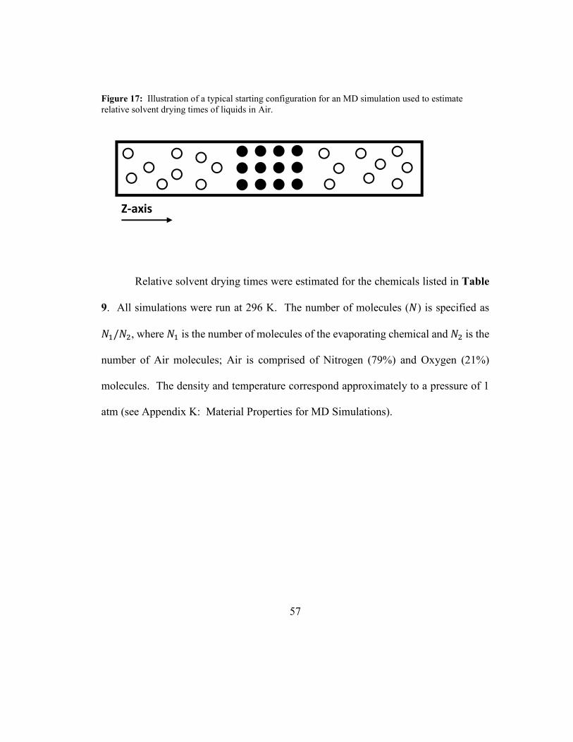
57

Figure 17: Illustration of a typical starting configuration for an MD simulation used to estimate

relative solvent drying times of liquids in Air.

Relative solvent drying times were estimated for the chemicals listed in Table

9. All simulations were run at 296 K. The number of molecules (�) is specified as

�o/�A, where �o is the number of molecules of the evaporating chemical and �A is the

number of Air molecules; Air is comprised of Nitrogen (79%) and Oxygen (21%)

molecules. The density and temperature correspond approximately to a pressure of 1

atm (see Appendix K: Material Properties for MD Simulations).

Z-axis

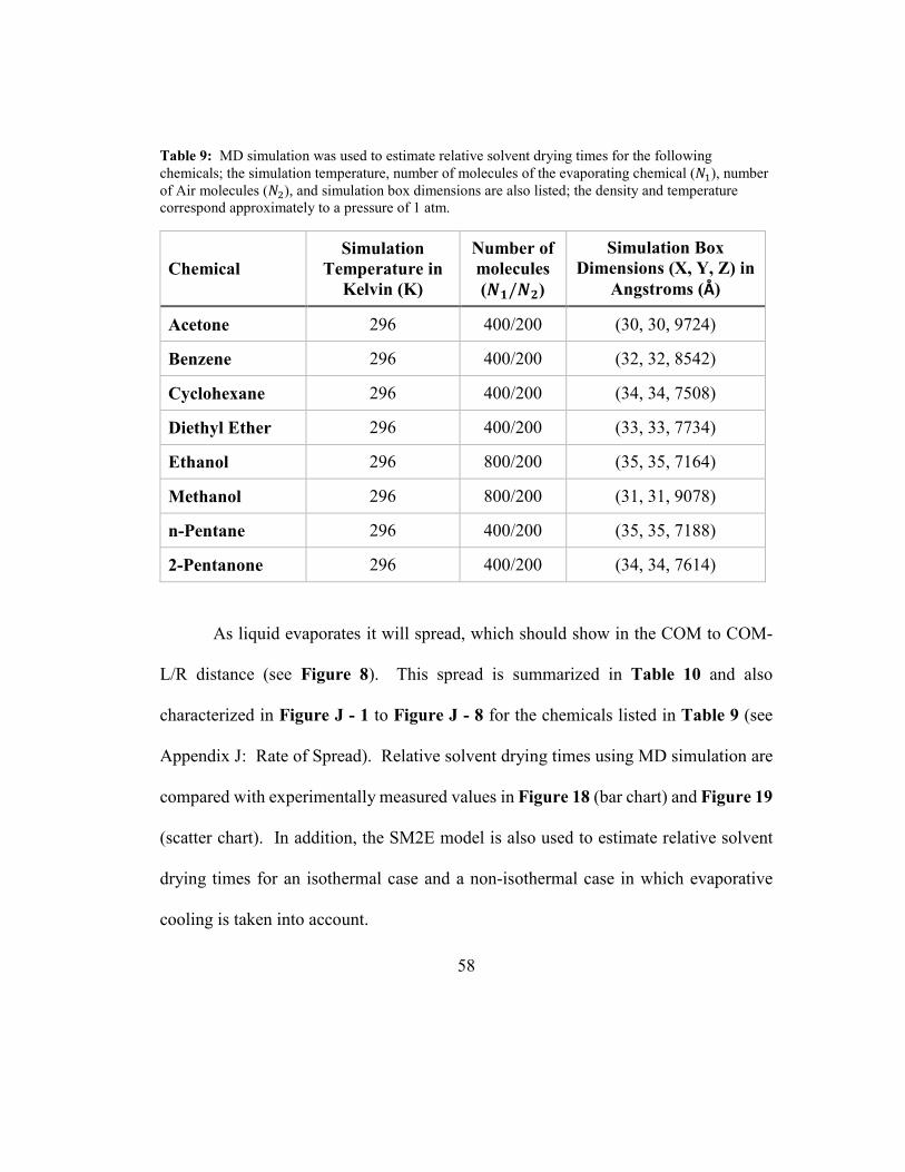
58

Table 9: MD simulation was used to estimate relative solvent drying times for the following

chemicals; the simulation temperature, number of molecules of the evaporating chemical (�o), number

of Air molecules (�A), and simulation box dimensions are also listed; the density and temperature

correspond approximately to a pressure of 1 atm.

Chemical

Simulation

Temperature in

Kelvin (K)

Number of

molecules

(��/��)

Simulation Box


Angstroms (Å)

Acetone 296 400/200 (30, 30, 9724)

Benzene 296 400/200 (32, 32, 8542)

Cyclohexane 296 400/200 (34, 34, 7508)

Diethyl Ether 296 400/200 (33, 33, 7734)

Ethanol 296 800/200 (35, 35, 7164)

Methanol 296 800/200 (31, 31, 9078)

n-Pentane 296 400/200 (35, 35, 7188)

2-Pentanone 296 400/200 (34, 34, 7614)

As liquid evaporates it will spread, which should show in the COM to COM-

L/R distance (see Figure 8). This spread is summarized in Table 10 and also

characterized in Figure J - 1 to Figure J - 8 for the chemicals listed in Table 9 (see

Appendix J: Rate of Spread). Relative solvent drying times using MD simulation are

compared with experimentally measured values in Figure 18 (bar chart) and Figure 19

(scatter chart). In addition, the SM2E model is also used to estimate relative solvent

drying times for an isothermal case and a non-isothermal case in which evaporative

cooling is taken into account.

59

Table 10: Average rate of solvent spread during liquid evaporation as measured from MD simulation;

see Figure 8 for an illustration; relative solvent drying times are estimated based on the average rate of

spread as shown in Equation (39).

Chemical Rate of Spread (cm/s)

Left Side Right Side

Acetone 5.542 4.367

Benzene 2.358 0.770

Cyclohexane 0.197 0.192

Diethyl Ether 8.356 4.809

Ethanol 0.521 0.464

Methanol 0.644 0.249

n-Pentane 7.569 9.964

2-Pentanone 0.006 0.015

60

Figure 18: Bar chart; relative solvent drying times at 296 K and 1 atm; MD simulation estimates are

compared with experimentally measured values.

61

Figure 19: Scatter chart; relative solvent drying times at 296 K and 1 atm; MD simulation estimates

are compared with experimentally measured values

This work was driven by a simple question. If MD simulation is used to

estimate relative solvent drying times of liquids into Air, how will these estimates

compare to experimentally measured values or modeled values?

One important observation from this work is that even for the relatively small

systems simulated in this work, in most cases, simulation times of 10 to 20 nanoseconds

(ns) are needed to adequately characterize the spread of the evaporating liquid.

62

In most cases, results from MD simulation are within an order of magnitude of

measured values. The notable exceptions are Cyclohexane and 2-Pentanone. This

observation is interesting because Benzene and Cyclohexane are both cyclic

compounds, while Acetone and 2-Pentanone are both Ketones. But the dynamics of

Cyclohexane and 2-Pentanone are observed to be much slower than Benzene and

Acetone, respectively (see Table 10); suggesting TraPPE intermolecular attractions

may be too strong.

Since the TraPPE potentials used in this work are optimized using phase

equilibria data, they may not be adequate for estimating transport properties such as

relative solvent drying times in all cases. This work starts to quantify the accuracy one

can expect when estimating transport properties such as relative evaporation rates from

potentials that have been parameterized using phase equilibria data.

Using the SM2E model yields more consistent results and does not require as

much computational effort. So why even explore MD simulation for estimating these

properties? Well, although it may be more practical to use the SM2E model for

estimation purposes, this work highlights an opportunity for developing potentials that

are parameterized using transport data and then assessing the performance of these

potentials when they are used to estimate equilibrium properties. Such potentials may

be better candidates for studying the dynamics of a system.

63

Appendix A: Example MDL Molfile Coordinate File (Methane)

The contents of an MDL Molfile for Methane are included in Table A - 1. The

first three lines constitute a header section. Line 1 specifies the molecule’s name,

which is “297” in this case. Line 2 says that the molecule was generated by “Marvin

12300703363D”. Line 3 is a comment line and in this case it is blank.

Line 4 is referred to as the “counts” line and identifies the number of atoms and

bonds in the molecule; 5 atoms and 4 bonds in this case. Lines 5-9 is the “Atom block”

and describes each atom's Cartesian coordinates (x, y, z) in angstroms and the atomic

symbol.

Lines 10-13 is the “Bonds block” and each line describes a bond. For example,

Line 10 identifies the atoms in the bond (atoms 1 and 2), and the bond type (bond type

“1” means single bond). Line 14 is the termination line.

Table A - 1: Contents of a Methane MDL Molfile obtained from ChemSpider.

1. 297 2. Marvin 12300703363D 3. 4. 5 4 0 0 0 0 999 V2000 5. -0.0000 -0.0000 0.0000 C 0 0 0 0 0 0 0 0 0 0 0 0 6. 1.0900 -0.0000 0.0000 H 0 0 0 0 0 0 0 0 0 0 0 0 7. -0.3633 1.0277 0.0000 H 0 0 0 0 0 0 0 0 0 0 0 0 8. -0.3633 -0.5138 0.8900 H 0 0 0 0 0 0 0 0 0 0 0 0 9. -0.3633 -0.5138 -0.8900 H 0 0 0 0 0 0 0 0 0 0 0 0 10. 1 2 1 0 0 0 0 11. 1 3 1 0 0 0 0 12. 1 4 1 0 0 0 0 13. 1 5 1 0 0 0 0 14. M END

64

Appendix B: Example PDB Coordinate File (Methane)

The contents of a PDB file for Methane are included in Table B - 1. Each line

represents a particular type of record. For example, REMARK records can contain

free-form explanations or comments; HETATM records list Cartesian coordinates (x,

y, z) in angstroms for hetero-atoms, atoms that are not part of a protein molecule;

CONECT records describe connectivity between atoms; and the END record marks the

end of the PDB file.

Table B - 1: Contents of a Methane PDB file obtained from Open Babel.

REMARK 1 2 3 4 5 6 7 8 REMARK789012345678901234567890123456789012345678901 23456789012345678901234567890 COMPND 297 AUTHOR GENERATED BY OPEN BABEL 2.3.2 HETATM 1 C1 MET 1 0.000 0.000 0. 000 1.00 0.00 C HETATM 2 H1 MET 1 1.090 0.000 0. 000 1.00 0.00 H HETATM 3 H2 MET 1 -0.363 1.028 0. 000 1.00 0.00 H HETATM 4 H3 MET 1 -0.363 -0.514 0. 890 1.00 0.00 H HETATM 5 H4 MET 1 -0.363 -0.514 -0. 890 1.00 0.00 H CONECT 1 2 3 4 5 CONECT 1 CONECT 2 1 CONECT 3 1 CONECT 4 1 CONECT 5 1 MASTER 0 0 0 0 0 0 0 0 5 0 5 0 END

65

Appendix C: Example PACKMOL Configuration Files

The PACKMOL input file used to prepare an initial configuration for estimating

diffusion for a gas mixture of Methane and Carbon Dioxide at approximately 298 K

and 1 atm is included in Table C - 1. This input file defines a rectangular box whose

dimensions are specified in Angstroms. Methane molecules are placed on one side of

the box and Carbon Dioxide molecules on the other side, creating a concentration

gradient along the Z axis.

Table C - 1: PACKMOL input file for estimating diffusion for a Methane-Carbon Dioxide gas

mixture at approximately 298 K and 1 atm; all dimensions are in Angstroms.

# Methane-CO2 Mixture at 298 K and 1 atm # All the atoms from different molecules will be se parated at least 2.0 # Angstroms at the solution. tolerance 2.0 # The file type of input and output files is PDB filetype pdb # Increase maximum system dimensions sidemax 5000.d0 # The name of the output file output mixture.pdb # Place molecules inside a box structure methane.pdb number 133 inside box 0.0 0.0 0.0 100.0 100.0 547.0 end structure structure carbon_dioxide.pdb number 133 inside box 0.0 0.0 -546.0 100.0 100. 0.0 end structure

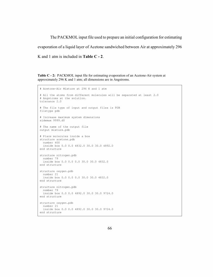
66

The PACKMOL input file used to prepare an initial configuration for estimating

evaporation of a liquid layer of Acetone sandwiched between Air at approximately 296

K and 1 atm is included in Table C - 2.

Table C - 2: PACKMOL input file for estimating evaporation of an Acetone-Air system at

approximately 296 K and 1 atm; all dimensions are in Angstroms.

# Acetone-Air Mixture at 296 K and 1 atm # All the atoms from different molecules will be se parated at least 2.0 # Angstroms at the solution. tolerance 2.0 # The file type of input and output files is PDB filetype pdb # Increase maximum system dimensions sidemax 9999.d0 # The name of the output file output mixture.pdb # Place molecules inside a box structure acetone.pdb number 400 inside box 0.0 0.0 4832.0 30.0 30.0 4892.0 end structure structure nitrogen.pdb number 79 inside box 0.0 0.0 0.0 30.0 30.0 4832.0 end structure structure oxygen.pdb number 21 inside box 0.0 0.0 0.0 30.0 30.0 4832.0 end structure structure nitrogen.pdb number 79 inside box 0.0 0.0 4892.0 30.0 30.0 9724.0 end structure structure oxygen.pdb number 21 inside box 0.0 0.0 4892.0 30.0 30.0 9724.0 end structure

67

Appendix D: NAMD Topology File

Table D - 1: NAMD topology file used for MD simulations.

! Atom Type MASS 1 CH4 16.04300 C ! CH4 pseudo atom , UA traPPE Alkanes MASS 2 CH3 15.03500 C ! CH3 pseudo atom , UA traPPE Alkanes MASS 3 CH2 14.02700 C ! CH2 pseudo atom , UA traPPE Alkanes MASS 4 CH 13.01900 C ! CH psuedo atom, UA traPPE Alkanes MASS 5 C 12.01100 C ! C pseudo atom, UA traPPE Alkanes MASS 6 OT 15.99940 O ! TIPS3P WATER OX YGEN MASS 7 HT 1.00800 H ! TIPS3P WATER HY DROGEN MASS 8 CS 12.01100 C ! C pseudo atom, traPPE-small CO2 MASS 9 OS 15.99940 O ! O pseudo atom, traPPE-small CO2 MASS 10 CK 12.01100 C ! C pseudo atom, UA traPPE ketone MASS 11 C3K 15.03500 C ! CH3 pseudo atom , UA traPPE ketone MASS 12 OK 15.99940 O ! O pseudo atom, UA traPPE ketone MASS 13 O2 10.66627 O ! O pseudo atom, traPPE-small O2 MASS 14 MO2 10.66627 M ! M (dummy) pseud o atom, traPPE-small O2 MASS 15 N2 9.33800 N ! N pseudo atom, traPPE-small N2 MASS 16 ZO2 9.33800 Z ! Z (dummy) pseud o atom, traPPE-small N2 MASS 17 EH3 15.03500 C ! CH3 pseudo atom , UA traPPE Ethers MASS 18 EH2 14.02700 C ! CH2 pseudo atom , UA traPPE Ethers MASS 19 EO 15.99940 O ! O pseudo atom, UA traPPE Ethers MASS 20 AO 15.99940 O ! O pseudo atom, UA traPPE Alcohols MASS 21 HA 1.00800 H ! H pseudo atom, UA traPPE Alcohols MASS 22 CC2 14.02700 C ! CH2 pseudo atom , UA traPPE Cyclic Alkanes MASS 23 C2K 14.02700 C ! CH2 pseudo atom , UA traPPE ketone MASS 24 ACH 13.01900 C ! CH psuedo atom, UA traPPE Aromatics DEFA FIRS NONE LAST NONE AUTO ANGLES DIHE RESI MET 0.000 ! Methane molecule GROUP ATOM C1 CH4 0.000 PATCHING FIRS NONE LAST NONE RESI ETH 0.000 ! Ethane molecule GROUP ATOM C1 CH3 0.000 ATOM C2 CH3 0.000 BOND C1 C2 PATCHING FIRS NONE LAST NONE RESI PRO 0.000 ! Propane molecule GROUP ATOM C1 CH2 0.000 ATOM C2 CH3 0.000 ATOM C3 CH3 0.000 BOND C1 C2 C1 C3 PATCHING FIRS NONE LAST NONE RESI MOH 0.000 ! Methanol molecule GROUP ATOM C1 CH3 0.265 ATOM O1 AO -0.700

68

ATOM H1 HA 0.435 BOND C1 O1 O1 H1 PATCHING FIRS NONE LAST NONE RESI EOH 0.000 ! Ethanol molecule GROUP ATOM C3 CH3 0.000 ATOM C2 CH2 0.265 ATOM O1 AO -0.700 ATOM H1 HA 0.435 BOND C3 C2 C2 O1 O1 H1 PATCHING FIRS NONE LAST NONE RESI BUT 0.000 ! n-butane molecule GROUP ATOM C1 CH3 0.000 ATOM C2 CH2 0.000 ATOM C3 CH2 0.000 ATOM C4 CH3 0.000 BOND C1 C2 C2 C3 C3 C4 PATCHING FIRS NONE LAST NONE RESI PEN 0.000 ! n-Pentane molecule GROUP ATOM C1 CH2 0.000 ATOM C2 CH2 0.000 ATOM C3 CH2 0.000 ATOM C4 CH3 0.000 ATOM C5 CH3 0.000 BOND C1 C2 C1 C3 C2 C4 C3 C5 PATCHING FIRS NONE LAST NONE RESI CHX 0.000 ! Cyclohexane molecule GROUP ATOM C1 CC2 0.000 ATOM C2 CC2 0.000 ATOM C3 CC2 0.000 ATOM C4 CC2 0.000 ATOM C5 CC2 0.000 ATOM C6 CC2 0.000 BOND C1 C2 C1 C3 C2 C4 C3 C5 C4 C6 C5 C6 PATCHING FIRS NONE LAST NONE RESI BNZ 0.000 ! Benzene molecule GROUP ATOM C1 ACH 0.000 ATOM C2 ACH 0.000 ATOM C3 ACH 0.000 ATOM C4 ACH 0.000 ATOM C5 ACH 0.000 ATOM C6 ACH 0.000 BOND C1 C3 C2 C4 C5 C6 DOUBLE C1 C2 C3 C5 C4 C6 PATCHING FIRS NONE LAST NONE RESI DEE 0.000 ! Diethyl Ether molecule GROUP ATOM O1 EO -0.500 ATOM C1 EH2 0.250 ATOM C2 EH2 0.250 ATOM C3 EH3 0.000

69

ATOM C4 EH3 0.000 BOND O1 C1 O1 C2 C1 C3 C2 C4 PATCHING FIRS NONE LAST NONE RESI CO2 0.000 ! Carbon Dioxide molecule GROUP ATOM C1 CS 0.700 ATOM O1 OS -0.350 ATOM O2 OS -0.350 BOND C1 O1 C1 O2 PATCHING FIRS NONE LAST NONE RESI ACE 0.000 ! Acetone molecule GROUP ATOM O1 OK -0.424 ATOM C1 CK 0.424 ATOM C2 C3K 0.000 ATOM C3 C3K 0.000 BOND C1 C2 C1 C3 DOUBLE C1 O1 PATCHING FIRS NONE LAST NONE RESI 2PN 0.000 ! 2-Pentanone molecule GROUP ATOM O1 OK -0.424 ATOM C1 CK 0.424 ATOM C2 C3K 0.000 ATOM C3 C2K 0.000 ATOM C4 C2K 0.000 ATOM C5 C3K 0.000 BOND C1 C2 C1 C3 C3 C4 C4 C5 DOUBLE C1 O1 PATCHING FIRS NONE LAST NONE RESI O2 0.000 ! Oxygen molecule GROUP ATOM O21 O2 -0.113 ATOM M1 MO2 0.226 ATOM O22 O2 -0.113 BOND O21 M1 M1 O22 PATCHING FIRS NONE LAST NONE RESI N2 0.000 ! Nitrogen molecule GROUP ATOM N21 N2 -0.482 ATOM Z1 ZO2 0.964 ATOM N22 N2 -0.482 BOND N21 Z1 Z1 N22 PATCHING FIRS NONE LAST NONE RESI TIP 0.000 ! tip3p water model, genera te using noangle nodihedral GROUP ATOM OH2 OT -0.834 ATOM H1 HT 0.417 ATOM H2 HT 0.417 BOND OH2 H1 OH2 H2 !!H1 H2 ! the last bond is needed for shake, but not in NAMD ANGLE H1 OH2 H2 ! required END

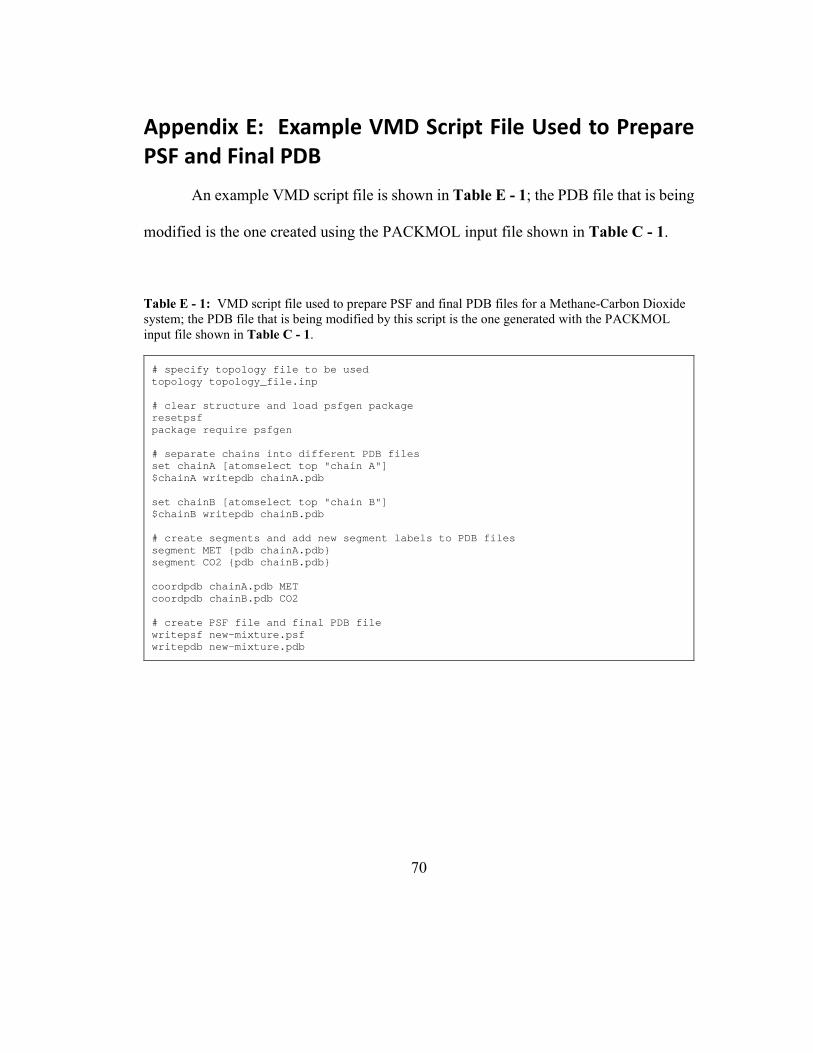
70

Appendix E: Example VMD Script File Used to Prepare PSF and Final PDB

An example VMD script file is shown in Table E - 1; the PDB file that is being

modified is the one created using the PACKMOL input file shown in Table C - 1.

Table E - 1: VMD script file used to prepare PSF and final PDB files for a Methane-Carbon Dioxide

system; the PDB file that is being modified by this script is the one generated with the PACKMOL

input file shown in Table C - 1.

# specify topology file to be used topology topology_file.inp # clear structure and load psfgen package resetpsf package require psfgen # separate chains into different PDB files set chainA [atomselect top "chain A"] $chainA writepdb chainA.pdb set chainB [atomselect top "chain B"] $chainB writepdb chainB.pdb # create segments and add new segment labels to PDB files segment MET {pdb chainA.pdb} segment CO2 {pdb chainB.pdb} coordpdb chainA.pdb MET coordpdb chainB.pdb CO2 # create PSF file and final PDB file writepsf new-mixture.psf writepdb new-mixture.pdb

71

Appendix F: NAMD Parameter File

Table F - 1: NAMD parameter file used for MD simulations.

BONDS ! !V(bond) = Kb(b - b0)**2 ! !Kb: kcal/mole/A**2 !b0: A ! !atom type Kb b0 ! !METHANE ! !ETHANE CH3 CH3 3000.00 1.540 ! !BENZENE ACH ACH 3000.00 1.400 ! !PROPANE CH3 CH2 3000.00 1.540 ! !CYCLOHEXANE CC2 CC2 3000.00 1.540 ! !2-METYLPROPANE CH3 CH 3000.00 1.540 ! !N-BUTANE CH2 CH2 3000.00 1.540 ! !DIETHYL ETHER EH3 EH2 3000.00 1.540 EH2 EO 3000.00 1.410 ! !METHANOL CH3 AO 3000.00 1.430 AO HA 3000.00 0.945 ! !ETHANOL CH2 AO 3000.00 1.430 ! !TIP3 OT HT 450.000 0.9572 ! !CARBON DIOXIDE OS CS 3000.00 1.1600 ! !ACETONE CK OK 3000.00 1.2290 CK C3K 3000.00 1.5200 ! !2-PENTANONE CK C2K 3000.00 1.5200 C2K C2K 3000.00 1.5400 C2K C3K 3000.00 1.5400

72

! !OXYGEN (O2) O2 MO2 3000.00 0.6050 ! !NITROGEN (N2) N2 ZO2 3000.00 0.5500 ANGLES ! !V(angle) = Ktheta(Theta - Theta0)**2 ! !V(Urey-Bradley) = Kub(S - S0)**2 ! !Ktheta: kcal/mole/rad**2 !Theta0: degrees !Kub: kcal/mole/A**2 (Urey-Bradley) !S0: A ! !atom types Ktheta Theta0 Kub S0 ! !METHANE ! !ETHANE ! !PROPANE CH3 CH2 CH3 62.07 114.0 ! !BENZENE ACH ACH ACH 3000. 120.0 ! !METHANOL CH3 AO HA 55.02 108.5 ! !ETHANOL CH3 CH2 AO 50.05 109.5 CH2 AO HA 55.02 108.5 ! !2-METHYLPROPANE CH3 CH CH3 62.07 112.0 ! !N-BUTANE CH3 CH2 CH2 62.07 114.0 CH2 CH2 CH3 62.07 114.0 ! !N-PENTANE CH2 CH2 CH2 62.07 114.0 ! !CYCLOHEXANE CC2 CC2 CC2 62.07 114.0 ! !DIETHYL ETHER EH3 EH2 EO 49.95 112.0 EH2 EO EH2 59.98 112.0 !EO EH2 EH3 49.95 112.0 ! !TIP3 HT OT HT 55.000 104.5200 ! !CARBON DIOXIDE OS CS OS 3000. 180.0

73

! !ACETONE OK CK C3K 62.07 121.4 C3K CK C3K 62.07 117.2 ! !2-PENTANONE C3K CK C2K 62.07 117.2 OK CK C3K 62.07 121.4 CK C2K C2K 62.07 114.0 OK CK C2K 62.07 121.4 C2K C2K C3K 62.07 114.0 ! !OXYGEN (O2) O2 MO2 O2 3000. 180.0 ! !NITROGEN (N2) N2 ZO2 N2 3000. 180.0 DIHEDRALS ! !V(dihedral) = Kchi(1 + cos(n(chi) - delta)) ! !Kchi: kcal/mole !n: multiplicity !delta: degrees ! !atom types Kchi n delta ! !METHANE ! !ETHANE ! !PROPANE ! !BENZENE ACH ACH ACH ACH 0.00 0 0.00 ACH ACH ACH ACH 0.00 1 0.00 ACH ACH ACH ACH 0.00 2 180.00 ACH ACH ACH ACH 0.00 3 0.00 ! !2-METHYLPROPANE ! !N-BUTANE CH3 CH2 CH2 CH3 0.00 0 0.00 CH3 CH2 CH2 CH3 0.71 1 0.00 CH3 CH2 CH2 CH3 -0.14 2 180.00 CH3 CH2 CH2 CH3 1.57 3 0.00 ! !ETHANOL CH3 CH2 AO HA 0.00 0 0.00 CH3 CH2 AO HA 0.42 1 0.00 CH3 CH2 AO HA -0.06 2 180.00 CH3 CH2 AO HA 0.37 3 0.00 ! !CYCLOHEXANE CC2 CC2 CC2 CC2 10.08 0 0.00 CC2 CC2 CC2 CC2 13.59 1 0.00 CC2 CC2 CC2 CC2 6.97 2 180.00 CC2 CC2 CC2 CC2 0.13 3 0.00 !

74

!N-PENTANE CH3 CH2 CH2 CH2 0.00 0 0.00 CH3 CH2 CH2 CH2 0.71 1 0.00 CH3 CH2 CH2 CH2 -0.14 2 180.00 CH3 CH2 CH2 CH2 1.57 3 0.00 !CH2 CH2 CH2 CH3 0.00 0 0.00 !CH2 CH2 CH2 CH3 0.71 1 0.00 !CH2 CH2 CH2 CH3 -0.14 2 180.00 !CH2 CH2 CH2 CH3 1.57 3 0.00 ! !DIETHLY ETHER !EH3 EH2 EO EH2 0.00 0 0.00 !EH3 EH2 EO EH2 1.44 1 0.00 !EH3 EH2 EO EH2 -0.33 2 180.00 !EH3 EH2 EO EH2 1.11 3 0.00 EH2 EO EH2 EH3 0.00 0 0.00 EH2 EO EH2 EH3 1.44 1 0.00 EH2 EO EH2 EH3 -0.33 2 180.00 EH2 EO EH2 EH3 1.11 3 0.00 ! !2-PENTANONE C3K CK C2K C2K -0.03 0 0.00 C3K CK C2K C2K 1.49 1 0.00 C3K CK C2K C2K 0.03 2 180.00 C3K CK C2K C2K 0.56 3 0.00 ! CK C2K C2K C3K 0.00 0 0.00 CK C2K C2K C3K 0.71 1 0.00 CK C2K C2K C3K -0.14 2 180.00 CK C2K C2K C3K 1.57 3 0.00 ! C2K C2K CK OK 4.04 0 0.00 C2K C2K CK OK -1.46 1 0.00 C2K C2K CK OK 0.11 2 180.00 C2K C2K CK OK -0.58 3 0.00 ! !CARBON DIOXIDE ! !ACETONE ! !OXYGEN ! !NITROGEN ! IMPROPER ! !V(improper) = Kpsi(psi - psi0)**2 ! !Kpsi: kcal/mole/rad**2 !psi0: degrees !note that the second column of numbers (0) is igno red ! !atom types Kpsi psi0 ! NONBONDED ! !V(Lennard-Jones) = Eps,i,j[(Rmin,i,j/ri,j)**12 - 2 (Rmin,i,j/ri,j)**6]

75

! !epsilon: kcal/mole, Eps,i,j = sqrt(eps,i * eps,j) !Rmin/2: A, Rmin,i,j = Rmin/2,i + Rmin/2,j ! !atom ignored epsilon Rmin/2 ignored e ps,1-4 Rmin/2,1-4 ! !traPPE CH4 CH4 0.000000 -0.293961 2.093392 ! !traPPE CH3 CH3 0.000000 -0.194650 2.104616 ! !traPPE CH2 CH2 0.000000 -0.091366 2.216863 ! !traPPE CH CH 0.000000 -0.019862 2.626561 ! !traPPE C C 0.000000 -0.000993 3.591879 ! !TIP3 HYDROGEN HT 0.000000 -0.046000 0.224500 !TIP2 OXYGEN OT 0.000000 -0.152100 1.768200 ! !traPPE small CO2 OXYGEN OS 0.000000 -0.156912 1.711755 ! !traPPE small CO2 CARBON CS 0.000000 -0.053628 1.571447 !traPPE UA ketone CK 0.000000 -0.079449 2.143903 C2K 0.000000 -0.091366 2.216863 C3K 0.000000 -0.194650 2.104616 OK 0.000000 -0.156912 1.711755 ! !traPPE small O2 OXYGEN O2 0.000000 -0.097325 1.694918 ! !traPPE small O2 M (dummy) MO2 0.000000 0.000000 0.000000 ! !traPPE small N2 OXYGEN N2 0.000000 -0.071504 1.857675 ! !traPPE small N2 Z (dummy) ZO2 0.000000 0.000000 0.000000 ! !traPPE UA Ethers CH3 EH3 0.000000 -0.194650 2.104616 ! !traPPE UA Ethers CH2 EH2 0.000000 -0.091366 2.216863 ! !traPPE UA Ethers O EO 0.000000 -0.109242 1.571447 ! !traPPE UA Alcohols O AO 0.000000 -0.184719 1.694918 !

76

!traPPE UA Alcohols H HA 0.000000 -0.000000 0.000000 ! !traPPE UA Cyclic Alkanes CC2 CC2 0.000000 -0.104277 2.194413 ! !traPPE UA Aromatics ACH ACH 0.000000 -0.100304 2.073749 END

77

Appendix G: Example NAMD Configuration Files

Table G - 1: NAMD configuration file used to simulate a Methane system for estimating self-

diffusion at 400 K and 1 atm.

################################################### ########## ## ADJUSTABLE PARAMETERS ## ################################################### ########## structure new-mixture.psf coordinates new-mixture.pdb set temperature 400. set outputname methane_methane firsttimestep 0 ################################################### ########## ## SIMULATION PARAMETERS ## ################################################### ########## # Input paraTypeCharmm on parameters parameter_file.inp temperature $temperature # Center of Mass Motion COMmotion no # Force-Field Parameters exclude 1-4 #1-4scaling 1.0 cutoff 14.0 switching on switchdist 12.0 pairlistdist 16.0 # Integrator Parameters timestep 2.0 ;# 2fs/step rigidBonds all ;# needed for 2fs steps nonbondedFreq 1 fullElectFrequency 2 stepspercycle 10 # Constant Temperature Control langevin on ;# do langevin dynamics langevinDamping 1 ;# damping coefficient (g amma) of 1/ps langevinTemp $temperature langevinHydrogen off ;# don't couple langevin bath to hydrogens # Periodic Boundary Conditions cellBasisVector1 100.0 0.0 0.0 cellBasisVector2 0.0 100.0 0.0 cellBasisVector3 0.0 0 1106.0 cellOrigin 0.0 0.0 0.0 wrapWater off ;# wrap water to central cell wrapAll off ;# wrap other molecules too

78

#PME (for full-system periodic electrostatics) PME yes # let NAMD determine grid PMEGridSpacing 1.0 # Output outputName $outputname restartfreq 100 ;# 500steps = every 1ps dcdfreq 100 velDCDfreq 100 xstFreq 100 outputEnergies 100 outputPressure 100 ################################################### ########## ## EXECUTION SCRIPT ## ################################################### ########## # Minimization minimize 1000 reinitvels $temperature run 1000000 ;# 2ns

79

Table G - 2: NAMD configuration file used to simulate a Methane-Carbon Dioxide system for

estimating binary gas diffusion at 298 K and 1 atm.

################################################### ########## ## ADJUSTABLE PARAMETERS ## ################################################### ########## structure new-mixture.psf coordinates new-mixture.pdb set temperature 298. set outputname methane_co2 firsttimestep 0 ################################################### ########## ## SIMULATION PARAMETERS ## ################################################### ########## # Input paraTypeCharmm on parameters parameter_file.inp temperature $temperature # Center of Mass Motion COMmotion no # Force-Field Parameters exclude 1-4 #1-4scaling 1.0 cutoff 14.0 switching on switchdist 12.0 pairlistdist 16.0 # Integrator Parameters timestep 2.0 ;# 2fs/step rigidBonds all ;# needed for 2fs steps nonbondedFreq 1 fullElectFrequency 2 stepspercycle 10 # Constant Temperature Control langevin on ;# do langevin dynamics langevinDamping 1 ;# damping coefficient (g amma) of 1/ps langevinTemp $temperature langevinHydrogen off ;# don't couple langevin bath to hydrogens # Periodic Boundary Conditions cellBasisVector1 100.0 0.0 0.0 cellBasisVector2 0.0 100.0 0.0 cellBasisVector3 0.0 0 1093.0 cellOrigin 0.0 0.0 0.0 wrapWater on ;# wrap water t o central cell wrapAll on ;# wrap other m olecules too

80

#PME (for full-system periodic electrostatics) PME yes # let NAMD determine grid PMEGridSpacing 1.0 # Output outputName $outputname restartfreq 100 ;# 500steps = every 1ps dcdfreq 100 velDCDfreq 100 xstFreq 100 outputEnergies 100 outputPressure 100 ################################################### ########## ## EXECUTION SCRIPT ## ################################################### ########## # Minimization minimize 1000 reinitvels $temperature run 1000000 ;# 2ns

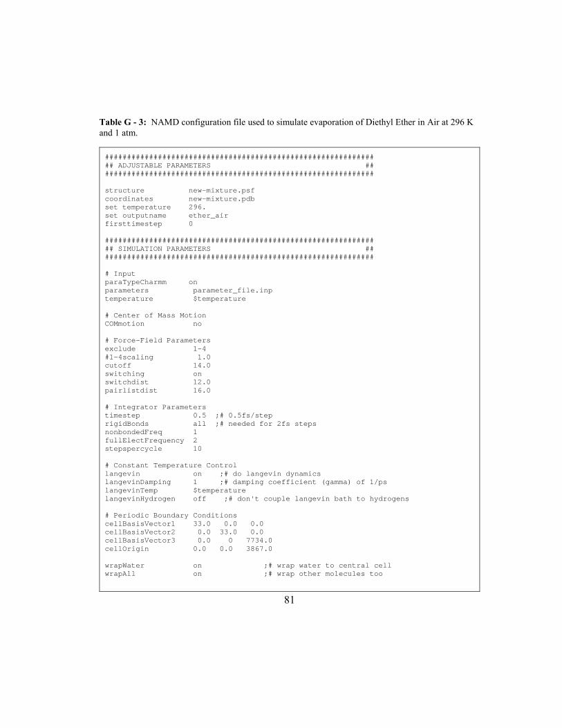
81

Table G - 3: NAMD configuration file used to simulate evaporation of Diethyl Ether in Air at 296 K

and 1 atm.

################################################### ########## ## ADJUSTABLE PARAMETERS ## ################################################### ########## structure new-mixture.psf coordinates new-mixture.pdb set temperature 296. set outputname ether_air firsttimestep 0 ################################################### ########## ## SIMULATION PARAMETERS ## ################################################### ########## # Input paraTypeCharmm on parameters parameter_file.inp temperature $temperature # Center of Mass Motion COMmotion no # Force-Field Parameters exclude 1-4 #1-4scaling 1.0 cutoff 14.0 switching on switchdist 12.0 pairlistdist 16.0 # Integrator Parameters timestep 0.5 ;# 0.5fs/step rigidBonds all ;# needed for 2fs steps nonbondedFreq 1 fullElectFrequency 2 stepspercycle 10 # Constant Temperature Control langevin on ;# do langevin dynamics langevinDamping 1 ;# damping coefficient (g amma) of 1/ps langevinTemp $temperature langevinHydrogen off ;# don't couple langevin bath to hydrogens # Periodic Boundary Conditions cellBasisVector1 33.0 0.0 0.0 cellBasisVector2 0.0 33.0 0.0 cellBasisVector3 0.0 0 7734.0 cellOrigin 0.0 0.0 3867.0 wrapWater on ;# wrap water t o central cell wrapAll on ;# wrap other m olecules too

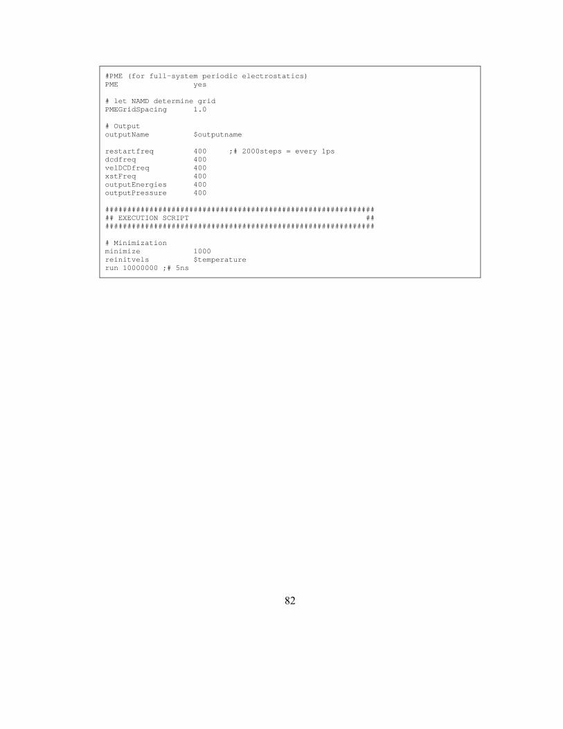
82

#PME (for full-system periodic electrostatics) PME yes # let NAMD determine grid PMEGridSpacing 1.0 # Output outputName $outputname restartfreq 400 ;# 2000steps = every 1p s dcdfreq 400 velDCDfreq 400 xstFreq 400 outputEnergies 400 outputPressure 400 ################################################### ########## ## EXECUTION SCRIPT ## ################################################### ########## # Minimization minimize 1000 reinitvels $temperature run 10000000 ;# 5ns

83

Appendix H: Example VMD Script Files for Trajectory Analysis

Table H - 1: VMD script file used to estimate the single particle mean square displacement for a pure

substance.

# Algorithm for calculating MSD (single particle) f or Pure Substance # Specify output file set outfile [open "msd_sp.dat" w] # Set molecules set molecule1 0 # Time step used for simulation set TimeStep 2.0e-15 # Steps per frame set FrameSteps 100. # Get number of frames set nf [molinfo $molecule1 get numframes] # Print labels puts $outfile "Frame Time_Delay MSD" # Time Start set TimeStart 1 # Time Origin Increment set TimeIncrement 10 # Starting Time Delay set StartingTimeDelay 1000 # Time Delay Increment set TimeDelayIncrement 500 # Loop over time delays for {set k $StartingTimeDelay} {$k < $nf} {incr k $ TimeDelayIncrement} { # Number of time origins available for given time d elay set T_origins [expr ($nf-$k+1)] # Initialize MSD_sp set MSD_sp 0.0 set TimeOrigins [expr {($T_origins - $TimeStart+1)/ $TimeIncrement}] # Loop over time origins for {set i $TimeStart} {$i < [expr ($nf-$k+1)]} {in cr i $TimeIncrement} { # Create two atom selections # Specify different frames for the two atom selecti ons # One at the time origin, the other at time origin plus time delay

84

set sel1 [atomselect $molecule1 "name OH2 and resna me TIP" frame [expr $i-1]] set sel2 [atomselect $molecule1 "name OH2 and resna me TIP" frame [expr $i-1+$k]] set coord1 [$sel1 get {x y z}] set coord2 [$sel2 get {x y z}] # Number of atoms in selection set N_atoms [$sel1 num] foreach coord1 $coord1 coord2 $coord2 { # Mean square displacement for given time delay ove r all time origins and atoms set MSD_sp [expr $MSD_sp + {[veclength2 [vecsub $co ord2 $coord1]]/$TimeOrigins/$N_atoms}] } # Delete selections $sel1 delete $sel2 delete } # Write to file: frame, time, MSD_sp puts $outfile "$k [expr $k*$FrameSteps*$TimeStep] $ MSD_sp" } #Close file close $outfile

85

Table H - 2: VMD script file used to estimate the collective mean square displacement for a Methane-

Carbon Dioxide System; the trajectory data being analyzed was generated using the NAMD

configuration file in Table G - 2.

# This file estimates collective mean square displa cement for a CH4 and CO2 system # Output file set outfile [open "msd_com.dat" w] # Molecules set molecule1 0 # Get number of frames set nf [molinfo $molecule1 get numframes] # Number of steps per frame set NS 100 # Time Step set TS [expr 2.0e-15] # Print labels puts $outfile "Frame Time_Delay MSD" # Loop over time delays for {set k 1} {$k <= $nf} {incr k 100} { # Number of time origins set T_origins [expr $nf-$k+1] # Estimate collective MSD set MSD 0.0 # Loop over time origins for {set i 1} {$i <= [expr ($nf-$k+1)]} {incr i 1} { # Select ch4 molecules set ch4_sel1 [atomselect $molecule1 "name C1 and re sname MET"] set ch4_sel2 [atomselect $molecule1 "name C1 and re sname MET"] # Select co2 molecules set co2_sel1 [atomselect $molecule1 "name C1 and re sname CO2"] set co2_sel2 [atomselect $molecule1 "name C1 and re sname CO2"] # Number of molecules set N_ch4 [$ch4_sel1 num] set N_co2 [$co2_sel1 num] set N_t [expr $N_ch4 + $N_co2] # Set frame for selection 1 $ch4_sel1 frame [expr $i-1] $co2_sel1 frame [expr $i-1] # Set frame for selection 2 $ch4_sel2 frame [expr $i+$k-1] $co2_sel2 frame [expr $i+$k-1] # Get center of mass for selections set ch4_com1 [measure center $ch4_sel1 weight mass] set co2_com1 [measure center $co2_sel1 weight mass]

86

set ch4_com2 [measure center $ch4_sel2 weight mass] set co2_com2 [measure center $co2_sel2 weight mass] # Center of mass separation in Z direction set j1 [expr {[lindex $ch4_com1 2]-[lindex $co2_com 1 2]}] set j2 [expr {[lindex $ch4_com2 2]-[lindex $co2_com 2 2]}] # Define a pre-factor set PF [expr {double($N_t)*0.5*0.5}] # Estimate mean square displacement for given time delay set MSD [expr $MSD + ($PF*($j2-$j1)*($j2-$j1)/doubl e($T_origins))] # Delete selections $ch4_sel1 delete $co2_sel1 delete $ch4_sel2 delete $co2_sel2 delete } # Write to file puts $outfile "$k [expr $k*$NS*$TS] [expr $MSD*1.0e -20]" } #Close file close $outfile

87

Table H - 3: VMD script file used to track how a liquid phase sandwiched between layers of Air

spreads with time.

# This file tracks the center of mass (COM) of liqu id molecules in Air # Output file set outfile [open "evap1.dat" w] # Print labels puts $outfile "Frame Time COM-COM_R COM-COM_L Area" # Molecules set molecule1 0 # PDB Velocity Factor, convert to A/ps set Vfactor 20.45482706 # Steps per Frame set StepsPerFrame 1600 # Time Step set TimeStep 0.5e-15 # Number of frames set nf [molinfo $molecule1 get numframes] # Unit cell dimensions X, Y, Z set X [molinfo $molecule1 get {a}] set Y [molinfo $molecule1 get {b}] set Z [molinfo $molecule1 get {c}] # Loop over frames for {set i 0} {$i <= $nf} {incr i} { # Center of mass of all liquid molecules set com_sel1 [atomselect $molecule1 "resname ACE" f rame $i] set COM [lindex [measure center $com_sel1 weight ma ss] 2] # Center of mass of liquid molecules with Z > COM set ACE1_sel1 [atomselect $molecule1 "resname ACE a nd z>$COM" frame $i] set N_ACE1 [$ACE1_sel1 num] set ACE1_COM [lindex [measure center $ACE1_sel1 wei ght mass] 2] # Center of mass of liquid molecules with Z < COM set ACE2_sel1 [atomselect $molecule1 "resname ACE a nd z<$COM" frame $i] set N_ACE2 [$ACE2_sel1 num] set ACE2_COM [lindex [measure center $ACE2_sel1 wei ght mass] 2] # Write to file puts $outfile "$i [expr $i*$StepsPerFrame*$TimeStep ] [expr {$ACE1_COM-$COM}] [expr {$ACE2_COM-$COM}] [expr $X*$Y]" # Delete selections $com_sel1 delete $ACE1_sel1 delete $ACE2_sel1 delete } #Close file close $outfile

89

Appendix I: Chapman-Enskog Theory

Based on Chapman-Enskog theory, the diffusion coefficient for gases can be

estimated using Equation (40), where �4� is the mutual diffusion coefficient of

molecules v and " in MA/c (or self-diffusion coefficient if v and " are the same

molecule), * is the absolute temperature in ��-, �4 and �� are the molecular

weights of molecules v and " in �/Mb�, $ is the pressure in =PM, �4� is the average

collision diameter of molecules v and " ��s��A � in v-�cPbMc, � is the collision

integral and is a function of the reduced temperature *� defined as � ∗¡¢�� , 0� is the

Boltzmann constant, and j4� is the geometric mean of the minimum potential values

for molecules v and " (√j4 ∗ j�). Collision diameters and minimum potential values

for relevant chemicals are listed in Table I - 1, while values for the collision integral

are listed in Table I - 2.

�4� = 1.858E-7 ∗ *¥A ∗ ¦ 1�4 + 1��$ ∗ �4�A ∗ �(*�) (40)

90

Table I - 1: Chapman-Enskog inputs; collision diameters and minimum potential values for relevant

chemicals.

Chemical Collision Diameter, §¨

(Angstroms)

Minimum Potential, ©¨/ª« (K)

Acetone 4.600 560.2

Carbon Dioxide 3.941 195.2

Methane 3.758 148.6

Propane 5.118 237.1

Water 2.641 809.1

Table I - 2: Chapman-Enskog inputs; values of the collision integral at various reduced temperatures.

Reduced Temperature ¬ = (ª« ∗ ¬)/©®¯ Collision Integral °(¬)

0.30 2.662

0.40 2.318

0.50 2.066

0.60 1.877

0.70 1.729

0.80 1.612

0.90 1.517

1.00 1.439

1.10 1.375

1.30 1.273

1.50 1.198

1.60 1.167

91

1.65 1.153

1.75 1.128

1.85 1.105

1.95 1.084

2.1 1.057

2.3 1.026

2.5 0.9996

2.7 0.9770

2.9 0.9576

3.3 0.9256

3.7 0.8998

3.9 0.8888

4.0 0.8836

4.2 0.8740

4.4 0.8652

4.6 0.8568

4.8 0.8492

5.0 0.8422

7 0.7896

9 0.7556

20 0.6640

60 0.5596

100 0.5130

300 0.4360

92

Appendix J: Rate of Spread

Figure J - 1: Spread of DIETHYL ETHER as it evaporates into Air at 296 K and 1 atm; rate of spread

can be estimated from the slope of the least-squares line.

93

Figure J - 2: Spread of ACETONE as it evaporates into Air at 296 K and 1 atm; rate of spread can be

estimated from the slope of the least-squares line.

94

Figure J - 3: Spread of ETHANOL as it evaporates into Air at 296 K and 1 atm; rate of spread can be


95

Figure J - 4: Spread of METHANOL as it evaporates into Air at 296 K and 1 atm; rate of spread can

be estimated from the slope of the least-squares line.

96

Figure J - 5: Spread of BENZENE as it evaporates into Air at 296 K and 1 atm; rate of spread can be


97

Figure J - 6: Spread of CYCLOHEXANE as it evaporates into Air at 296 K and 1 atm; rate of spread


98

Figure J - 7: Spread of N-PENTANE as it evaporates into Air at 296 K and 1 atm; rate of spread can

be estimated from the slope of the least-squares line.

99

Figure J - 8: Spread of 2-PENTANONE as it evaporates into Air at 296 K and 1 atm; rate fo spread


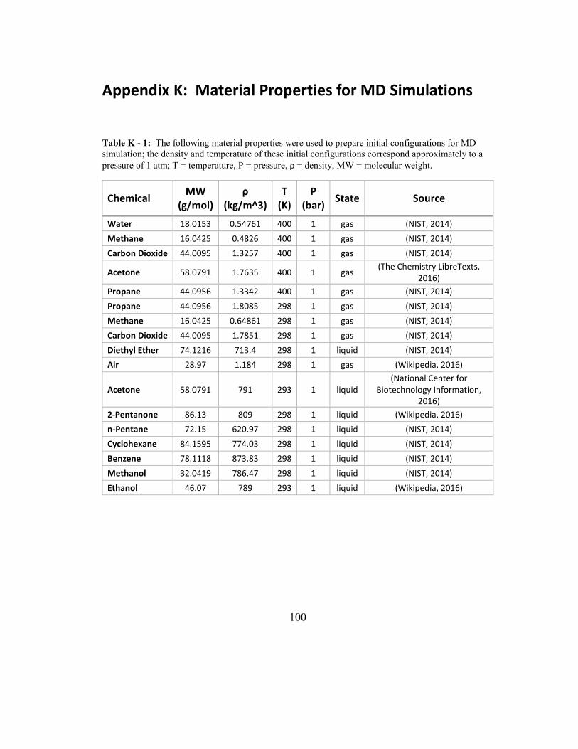
100

Appendix K: Material Properties for MD Simulations

Table K - 1: The following material properties were used to prepare initial configurations for MD

simulation; the density and temperature of these initial configurations correspond approximately to a

pressure of 1 atm; T = temperature, P = pressure, ρ = density, MW = molecular weight.

Chemical MW

(g/mol) ρ

(kg/m^3) T

(K) P

(bar) State Source

Water 18.0153 0.54761 400 1 gas (NIST, 2014)

Methane 16.0425 0.4826 400 1 gas (NIST, 2014)

Carbon Dioxide 44.0095 1.3257 400 1 gas (NIST, 2014)

Acetone 58.0791 1.7635 400 1 gas (The Chemistry LibreTexts,

2016)

Propane 44.0956 1.3342 400 1 gas (NIST, 2014)

Propane 44.0956 1.8085 298 1 gas (NIST, 2014)

Methane 16.0425 0.64861 298 1 gas (NIST, 2014)

Carbon Dioxide 44.0095 1.7851 298 1 gas (NIST, 2014)

Diethyl Ether 74.1216 713.4 298 1 liquid (NIST, 2014)

Air 28.97 1.184 298 1 gas (Wikipedia, 2016)

Acetone 58.0791 791 293 1 liquid (National Center for

Biotechnology Information, 2016)

2-Pentanone 86.13 809 298 1 liquid (Wikipedia, 2016)

n-Pentane 72.15 620.97 298 1 liquid (NIST, 2014)

Cyclohexane 84.1595 774.03 298 1 liquid (NIST, 2014)

Benzene 78.1118 873.83 298 1 liquid (NIST, 2014)

Methanol 32.0419 786.47 298 1 liquid (NIST, 2014)

Ethanol 46.07 789 293 1 liquid (Wikipedia, 2016)

101

Bibliography

Arnold, F. and Engel, A.J. 2001. Evaporation of pure liquids from open surfaces.

[book auth.] J.B.H.J. Linders. Modelling of Environmental Chemical Exposures and

Risk. s.l. : Springer, 2001, pp. 61-71.

Barry, J. 1995. Estimating rates of spreading and evaporation of volatile liquids.

Chemical Engineering Progress. 1995, pp. 32-39.

Braun, K.O. and Caplan, K.J. 1989. Evaporation rate of volatile liquids. Final

report. Second edition. Minneapolis : Pace Labs, Inc., 1989.

Chae, K. and Violi, A. 2011. Mutual diffusion coefficients of heptane isomers in

nitrogen: A molecular dynamics study. J. Chem. Phys. 2011, Vol. 134, 4.

Choudhary, R., Klauda, J.B. 2016. The simultaneous mass and energy evaporation

(SM2E) model. Journal of Occupational and Environmental Hygiene. 2016, Vol. 13,

4.

Consolini, L., Aggarwal, S.K. and Murad, S. 2003. A molecular dynamics simulation

of droplet evaporation. International Journal of Heat and Mass Transfer. 2003, Vol.

46.

Cussler, E. L. 2009. Diffusion: Mass Transfer In Fluid Systems, 3rd edition. New

York : Cambridge University Press, 2009. pp. 118-119. Table 5.1-1; we used the 14

diffusion coefficients in air.

Fehrenbacher, M.C. and Hummel, A.A. 1996. Evaluation of the mass balance model

used by the environmental protection agency for estimating inhalation exposure to new

chemical substances. AIHA Journal. 1996, pp. 526-536.

Fredenslund, A., Jones, R.L. and Prausnitz, J.M. 1975. Group-contribution

estimation of activity coefficients in nonideal liquid mixtures. AIChE Journal. 1975.

Gajjar, R.M., Miller, M.A. and Kasting, G.B. 2013. Evaporation of volatile organic

compounds from human skin in vitro. Ann. Occup. Hyg. 2013, pp. 853-865.

Haile, J. M. 1992. Molecular Dynamics Simulation: Elementary Methods. New York :

Jonh Wiley & Sons, INc., 1992. 0471819662.

102

Hansen, H.K., et al. 1991. Vapor-liquid equilibria by UNIFAC group contribution. 5.

Revision and extension. Ind. Eng. Chem. Res. 1991, pp. 2352-2355.

Hummel, A., Braun, K.O. and Fehrenbacher, M.C. 1996. Evaporation of a liquid in

a flowing airstream. AIHA Journal. 1996, pp. 519-525.

Humphrey, W., Dalke, A. and Schulten, K. 1996. VMD - Visual Molecular

Dynamics. Journal of Molecular Graphics. 1996, Vol. 14.

Jayjock, M., Armstrong, T. and Taylor, M. 2011. The Daubert standard as applied

to exposure assessment modeling using the two-zone (NF/FF) model estimation of

indoor air breathing zone conentration as an example. Journal of Occupational and

Environmental Hygiene. 2011, pp. D114-D122.

Jorgensen, W.L., Chandrasekhar, J. and Madura, J.D. 1983. Comparison of simple

potential functions for simulating liquid water. The Journal of Chemical Physics. 1983,

Vol. 79, 2.

Keil, C.B., Nicas, M. 2003. Predicting room vapor concentrations due to spills of

organic solvents. AIHA Journal. 2003, pp. 445-454.

Knovel. 2013. Yaws' Handbook of Antoine Coefficients for Vapor Pressure, 2nd

electronic edition. July 13, 2013.

Leach, A. R. 2001. Molecular Modelling: Principles and Applications (Second

Edition). New York : Pearson Prentice Hall, 2001. 9780582382107.

Long, L.N., Micci, M.M. and Wong, B.C. 1996. Molecular dynamics simulations of

droplet evaporation. Computer Physics Communications. 1996, Vol. 96.

Mackay, D. and Matsugu, R.S. 1973. Evaporation rates of liquid hydrocarbon spills

on land and water. The Canadian Journal of Chemical Engineering. 1973, pp. 434-439.

Makrodimitri, Z.A., Unruh, D.J.M. and Economou, I.G. 2011. Molecular

Simulations of Diffusion of Hydrogen, Carbon Monoxide, and Water in Heavy n-

Alkanes. J. Phys. Chem. B. 2011, Vol. 115.

Martinez, L., et al. 2009. Packmol: A package for building initial configurations for

molecular dynamics simulations. Journal of Computational Chemistry. 2009, Vol. 30,

13.

Middleman, S. 1998. An introduction to fluid dynamics: principles of analysis and

design. New York : John Wiley & Sons, Inc., 1998.

103

—. 1998. An introduction to mass and heat transfer: principles of analysis and design.

New York : John Wiley & Sons, Inc., 1998.

National Center for Biotechnology Information. 2016. Acetone. PubChem

Compound Database. [Online] 2016.

https://pubchem.ncbi.nlm.nih.gov/compound/acetone.

Nielsen, F., Olsen, E. and Fredunslund, A. 1995. Prediction of isothermal

evaporation rates of pure volatile organic compounds in occupational environments - a

theoretical approach based on laminar boundary layer theory. Ann. Occup. Hyg. 1995,

pp. 497-511.

NIST. 2014. NIST Chemistry WebBook. [Online] December 31, 2014.

http://webbook.nist.gov/chemistry/.

O'Boyle, N.M., et al. 2011. Open Babel: An open chemical toolbox. Journal of

Cheminformatics. 2011, Vol. 3.

Okamoto, K., et al. 2010. Evaporation characteristics of multi-component liquid.

Journal of Loss Prevention in the Process Industries. 2010, pp. 89-97.

Olsen, E. and Nielsen, F. 1995. On the prediction of evaporation rates - with special

emphasis on aqueous solutions. Ann. Occup. Hyg. 1995, pp. 513-522.

Phillips, J.C., et al. 2005. Scalable molecular dynamics with NAMD. Journal of

Computational Chemistry. 2005, Vol. 26, 16.

Poling, B.E., Prausnitz, J.M. and O'Connell, J.P. 2001. The Properties of Gases and

Liquids (Fifth Edition). New York : The McGraw-Hill Companies, Inc., 2001. 0-07-

149999-7.

Randhol, P. and Engelien, H.K. 2014. XLUNIFAC version 1.0. XLUNIFAC. [Online]

December 10, 2014. http://www.pvv.org/~randhol/xlunifac/.

Reinke, P.H., Brosseau, L.M. 1997. Development of a model to predict air

contaminant concentrations following indoor spills of volatile liquids. Ann occup. Hyg.

1997, pp. 415-435.

Royal Society of Chemistry. 2015. ChemSpider: Search and share chemistry.

[Online] 2015. http://www.chemspider.com/.

Sawhney, G.S. 2010. Heat and Mass Transfer, Second Edition. s.l. : I K International

Publishing House, 2010.

104

Sharma, R., Tankeshwar, K. and Ranganathan, S. 2011. Mass Dependence of

Mutual Diffusion Coefficient: Computer Simulation Study. Physics and Chemistry of

Liquids. 2011, Vol. 49, No. 2.

Smith, J.M., Van Ness, H.C. and Abbott, M.M. 2005. Introduction to chemical

engineering thermodynamics, 7th edition. Boston : McGraw-Hill, 2005.

Smith, R.L. 2001. Predicting evaporation rates and times for spills of chemical

mixtures. Ann. Occup. Hyg. 2001, pp. 437-445.

The Chemistry LibreTexts. 2016. A8: van der Waal's Constants for Real Gases.

[Online] 2016.

http://chem.libretexts.org/Reference/Reference_Tables/Atomic_and_Molecular_Prop

erties/A8%3A_van_der_Waal's_Constants_for_Real_Gases.

The Engineering ToolBox. 2014. Air Properties. Engineering Tool Box. [Online]

December 31, 2014. http://www.engineeringtoolbox.com/air-properties-d_156.html.

The Siepmann Group. 2015. TraPPE: Transferable Potentials for Phase Equilibria

Force Field. [Online] 2015. http://chem-

siepmann.oit.umn.edu/siepmann/trappe/index.html.

U.S. EPA. 2014. Technology Transfer Network Air Toxics Web site. Xylenes |

Technology Transfer Network Air Toxics Web site. [Online] December 31, 2014.

http://www.epa.gov/ttnatw01/hlthef/xylenes.html.

UNIFAC Consortium. Model Comparison. UNIFAC Consortium. [Online] [Cited:

July 30, 2015.] http://unifac.ddbst.de/model-comparison.html.

Wikipedia. 2016. 2-Pentanone. [Online] 2016. https://en.wikipedia.org/wiki/2-

Pentanone.

—. 2016. Density of air. [Online] 2016. https://en.wikipedia.org/wiki/Density_of_air.

—. 2016. Ethanol. [Online] 2016. https://en.wikipedia.org/wiki/Ethanol.

Wilson, L.D. 1955. Evaporation Rates of Solvents and an Improved Method for their

Determination. Paint, Oil and Chemical Review. 1955, Vol. 118, 24.

Yang, T.H. and Pan, C. 2005. Molecular dynamics simulation of a thin water layer

evaporation and evaporation coefficient. International Journal of Heat and Mass

Transfer. 2005, Vol. 48.

105

Yu, J. and Wang, H. 2012. A molecular dynamics investigation on evaporation of thin

liquid films. International Journal of Heat and Mass Transfer. 2012, Vol. 55.

Zhou, Y. and Miller, G.H. 1996. Green-Kubo Formulas for Mutual Diffusion

Coefficients in Multicomponent Systems. J. Phys. Chem. 1996, Vol. 100, 13.

Zhou, Z., et al. 2005. A molecular dynamics study of nitric oxide in water: Diffusion

and structure. The Journal of Chemical Physics. 2005, Vol. 123, 5.

106

List of Publications

Publications that have appeared in print

� Choudhary, R., Klauda, J.B. The Simultaneous Mass and Energy Evaporation

(SM2E) Model. Journal of Occupational and Environmental Hygiene. 2015, pp.

243-253. http://dx.doi.org/10.1080/15459624.2015.1101123

MODELING LIQUID EVAPORATION AND USING ...

Documents

Transcript of MODELING LIQUID EVAPORATION AND USING ...