Experimental investigation of water evaporation from sand ...
340
HAL Id: tel-01127303 https://pastel.archives-ouvertes.fr/tel-01127303 Submitted on 7 Mar 2015 HAL is a multi-disciplinary open access archive for the deposit and dissemination of sci- entific research documents, whether they are pub- lished or not. The documents may come from teaching and research institutions in France or abroad, or from public or private research centers. L’archive ouverte pluridisciplinaire HAL, est destinée au dépôt et à la diffusion de documents scientifiques de niveau recherche, publiés ou non, émanant des établissements d’enseignement et de recherche français ou étrangers, des laboratoires publics ou privés. Experimental investigation of water evaporation from sand and clay using an environmental chamber Weikang Song To cite this version: Weikang Song. Experimental investigation of water evaporation from sand and clay using an envi- ronmental chamber. Materials. Université Paris-Est, 2014. English. NNT : 2014PEST1047. tel- 01127303
-
Upload
khangminh22 -
Category
Documents
-
view
1 -
download
0
Transcript of Experimental investigation of water evaporation from sand ...

HAL Id: tel-01127303https://pastel.archives-ouvertes.fr/tel-01127303
Submitted on 7 Mar 2015
HAL is a multi-disciplinary open accessarchive for the deposit and dissemination of sci-entific research documents, whether they are pub-lished or not. The documents may come fromteaching and research institutions in France orabroad, or from public or private research centers.
L’archive ouverte pluridisciplinaire HAL, estdestinée au dépôt et à la diffusion de documentsscientifiques de niveau recherche, publiés ou non,émanant des établissements d’enseignement et derecherche français ou étrangers, des laboratoirespublics ou privés.
Experimental investigation of water evaporation fromsand and clay using an environmental chamber
Weikang Song
To cite this version:Weikang Song. Experimental investigation of water evaporation from sand and clay using an envi-ronmental chamber. Materials. Université Paris-Est, 2014. English. �NNT : 2014PEST1047�. �tel-01127303�

THESE
Pour obtenir le grade de
Docteur de l’Université Paris-Est
Discipline : Géotechnique
Présentée par
Weikang SONG
Experimental investigation of water evaporation from sand
and clay using an environmental chamber
Soutenue le lundi 10 Mars 2014 devant le jury composé de:
Prof. Pierre-Yves HICHER Ecole Centrale de Nantes Rapporteur Prof. De’an SUN Shanghai University Rapporteur
Prof. Liangtong ZHAN Zhejiang University Examinateur
Prof. Weimin YE Tongji University Examinateur
Prof. Yu-Jun CUI Ecole des Ponts ParisTech Directeur de thèse
Prof. Wenqi DING Tongji University Co-Directeur de thèse


To my parents


I
Résumé
Titre: Etude d'évaporation d'eau d'un sable et d'une argile à l'aide d'une chambre environnementale Il est bien connu que l'évaporation d'eau joue un rôle essentiel dans l'interaction entre
le sol et l'atmosphère. Pendant le processus d'évaporation, le comportement
thermo-hydro-mécanique des sols change, engendrant ainsi des problèmes
préoccupants. Ceci peut concerner différents domaines comme l'agronomie,
l'hydrologie, la science des sols, la géotechnique, etc. Par conséquent, il est essentiel
d'étudier les mécanismes d'évaporation de façon approfondie.
Cette étude porte sur les mécanismes d'évaporation dans des conditions
atmosphériques contrôlées. Le sable de Fontainebleau et l'argile d’Héricourt utilisée
pour la construction du remblai expérimental dans le cadre du projet ANR
TerDOUEST (Terrassements Durables - Ouvrages en Sols Traités, 2008-2012) ont été
étudiés à cet effet. Une chambre environnementale (900 mm de haut, 800 mm de large
et 1000 mm de long) équipée de différents capteurs a d'abord été développée,
permettant un suivi complet des paramètres concernant l'atmosphère et le sol au cours
d'évaporation.
Quatre essais expérimentaux ont été réalisés sur le sable de Fontainebleau compacté à
une densité sèche de 1,70 Mg/m3, avec une nappe phréatique constante au fond de
l'échantillon, et sous différentes conditions atmosphériques (différentes valeurs de
l'humidité relative de l'air, de la température et du débit d'air). La pertinence du
système a été mise en évidence par la bonne qualité des résultats. La température de
l'air à l'intérieur de la chambre a été trouvée affectée par la température du tube de
chauffage, le débit d'air et l'évaporation d’eau; la température du sol est fortement
affectée par les conditions atmosphériques et l'état d'avancement de l'évaporation;
l'humidité relative dans la chambre diminue au cours du temps et son évolution peut
être considérée comme un indicateur du processus d'évaporation; la teneur en eau
volumique dans la zone proche de la surface est fortement influencée par le processus
d'évaporation et présente une relation linéaire avec la profondeur; la succion du sol

II
diminue avec la profondeur et augmente au fil du temps; le taux d'évaporation est
fortement affecté par les conditions de l'air en particulier dans la phase initiale de
vitesse d'évaporation constante.
Après les essais sur le sable de Fontainebleau, l'échantillon de l'argile d'Héricourt
compactée à une densité sèche de 1,40 Mg/m3 a été soumis à une infiltration d’eau
afin d'étudier ses propriétés hydrauliques. Pour obtenir un meilleur aperçu du
mécanisme d'évaporation pour l'argile, deux essais d'évaporation sur l'argile
d'Héricourt compactée avec une nappe phréatique constante au fond de l’échantillon
ont été effectuées sous des conditions atmosphériques contrôlées. Les résultats
permettent de comprendre les mécanismes d'évaporation en cas de fissuration due à la
dessiccation. En outre, afin d'étudier les mécanismes d'évaporation potentiels, des
essais avec une couche d'eau libre ont été également réalisés en faisant varier la
vitesse du vent et la température de l'air. L'initiation et la propagation de fissures de
dessiccation pendant le processus d'évaporation et son effet sur l'évaporation ont
également été étudiés par la technique de traitement d'image.
En termes de modélisation, le taux d'évaporation potentiel a été modélisé à travers
l'évaluation des modèles existants et des modèles combinés. Il apparait que le modèle
développé par Ta (2009) est le plus approprié. Le taux d'évaporation réelle depuis le
sable a été ensuite analysé. Il semble important de considérer l'avancement du front
sec pendant le processus d'évaporation pour les sols sableux. Pour l'argile d'Héricourt,
une bonne prévision a été également obtenue en utilisant un modèle qui tient compte
de l'effet des fissures de dessiccation.
Mots clés: mécanism d'évaporation; sable; argile; chambre environnementale;
conditions atmosphérique; fissuration de dessicccation; évaporation potentielle;
évaporation réelle; modèle d'évaporation

III
Abstract
Title: Experimental investigation of water evaporation from sand and clay using an environmental chamber As a well-known phenomenon, soil water evaporation plays an important role in the
interaction between soil and atmosphere. Water evaporates during this process
resulting in changes of soil thermo-hydro-mechanical behavior and in turn causing
problems in different domains such as agronomy, hydrology, soil science,
geotechnical engineering, etc. Therefore, it is essential to investigate the soil water
evaporation mechanisms in depth.
This study deals with the soil water evaporation mechanisms under controlled
atmospheric conditions. The Fontainebleau sand and the Héricourt clay used for the
construction of the experimental embankment with the ANR project TerDOUEST
(Terrassements Durables - Ouvrages en Sols Traités, 2008 - 2012) were used in this
investigation. A large-scale environmental chamber system (900 mm high, 800 mm
large and 1000 mm long) equipped with various sensors was firstly developed,
allowing a full monitoring of both atmospheric and soil parameters during the
evaporation process.
Four experimental tests were carried out on the Fontainebleau sand compacted at
1.70 Mg/m3 dry density with a steady water table at soil bottom under different
atmospheric conditions (different values of air relative humidity, temperature and air
flow rate). The performance of the environmental chamber system in investigating
soil water evaporation was evidenced by the quality and the relevance of results. The
air temperature inside the chamber was found to be affected by the heating tube
temperature, the air flow rate and the soil water evaporation process; the soil
temperature was strongly affected by the air conditions and the evaporation progress;
the relative humidity in the chamber was decreasing during the evaporation progress
and its evolution could be considered as an indicator of the evaporation progress; the
volumetric water content in the near-surface zone was strongly affected by the
evaporation process and exhibited a linear relationship with depth; the soil suction

IV
was decreasing over depth and increasing over time; the evaporation rate was strongly
affected by the air conditions especially at the initial constant evaporation rate stage.
After the tests on the Fontainebleau sand, the Héricourt clay sample compacted at
1.40 Mg/m3 dry density was subjected to an infiltration experiment for investigating
its hydraulic properties. To get a better insight into the water evaporation mechanism
for clay, two compacted Héricourt clay evaporation tests with a steady water table at
bottom were carried out under controlled atmospheric conditions. The results allow
understanding the evaporation mechanisms in case of desiccation cracks. Furthermore,
in order to investigate the potential evaporation mechanisms, tests with a free water
layer was also conducted with varying wind speed and air temperature. The initiation
and propagation of desiccation cracking during the evaporation process and its effect
on water evaporation were also investigated by the digital image processing
technique.
In terms of modeling, the potential evaporation rate was first modeled through
evaluation of the existing models and the combined models. It reveals that the model
developed by Ta (2009) is the most appropriate one. The actual evaporation rate for
sand was then analyzed. It appears important to consider the progress of the dry front
during the evaporation process for sandy soils. For the Héricourt clay, good
simulation was also obtained using a model that accounts for the effect of desiccations
cracks.
Keywords: evaporation mechanism; sand; clay; environmental chamber;
atmospheric conditions; desiccation cracking; potential evaporation; actual
evaporation; evaporation model

V
摘 要
题目:砂土与粘土水分蒸发机理的环境箱试验研究
众所周知,土体水分蒸发是土与大气交互作用过程中的一个重要环节。在这
个过程中,土中水分的蒸发引起了土体热-水力-力学性质的变化,从而在诸如农
学、水文学、土壤学和岩土工程等领域引起了各种各样的问题。因此,对土体水
分的蒸发机理进行研究至关重要。
本文主要对控制大气条件下土体水分的蒸发机理进行研究。所采用试验材料
为 Fontainebleau 砂土和用于法国基金委(ANR)项目 TerDOUEST(Terrassements
Durables - Ouvrages en Sols Traités, 2008-2012)中试验路堤建设的 Héricourt 粘土。
为了能够对蒸发过程中的大气和土体参数进行全方位的监测,本文开发了一个配
备多种传感器的大体积环境箱蒸发测量系统(尺寸:1000 mm 长,800 mm 宽,
900 mm 高)。随后进行了 4 组不同大气条件下(不同相对湿度、不同温度和空气
流量)底部保持稳定水位的大体积压实 Fontainebleau 砂土(干密度 1.7 g/cm3)
蒸发试验。高质量的试验结果验证了环境箱蒸发测量系统的工作性能。研究结果
还表明:环境箱内空气温度的变化受到加热管温度、空气流量和土体水分蒸发过
程的影响;土体温度的变化也深受大气条件和蒸发过程的影响;在蒸发过程中,
环境箱内空气的相对湿度随着蒸发的进行逐渐降低,它的变化可以看作蒸发过程
的一个指示器;表层区域内土体体积含水量的变化受蒸发过程的影响较大;其分
布与土体深度呈线性关系;土体吸力沿着深度方向逐渐降低,但随蒸发时间的增
加而增大;蒸发速率特别是在初始常速率阶段受到大气条件变化的影响较大。而
后,为了研究 Héricourt 粘土的水力性质,在该环境箱内进行了大体积压实
Héricourt 粘土(干密度为 1.4 g/cm3)的渗透试验。此外,为了更加深入地对粘
性土土体水分蒸发机理进行研究,在渗透试验结束后,又进行了 2 组保持土体底
部稳定水位、控制大气条件的 Héricourt 粘土水分蒸发试验。该试验研究结果可
以加深对龟裂条件下土体水分蒸发机理的理解。为了研究潜在蒸发的机理,在该
环境箱内进行了自由水面在不同风速和空气温度条件下的蒸发试验。另一方面,
通过数字图像处理技术对水分蒸发过程中龟裂的开始与演化,以及龟裂对蒸发过
程的影响进行了研究。最后,在蒸发试验的基础上对蒸发速率的计算模型进行研
究。对潜在蒸发而言,本文通过对已有的计算模型及不同模型的组合的研究,验
证了 Ta(2009)所提出的模型的适用性。针对砂土水分蒸发的特点,本文提出
并验证了一个可以考虑蒸发过程中干燥面变化的蒸发速率计算模型。此外,通过
对粘土水分蒸发机理的研究,本文建立并验证了一个新的能够考虑龟裂影响的蒸

VI
发速率计算模型。 关键词:蒸发机理,砂土,粘土,环境箱,大气条件,龟裂,潜在蒸发,实际蒸
发,蒸发模型

VII
Acknowledgements
My deepest gratitude goes first and foremost to Prof. Yu-Jun Cui, my supervisor at
Ecole des Ponts ParisTech and Universite Paris-Est, for his constant encouragement
and guidance during the whole period of this dissertation. Without his profound
scientific vision, valuable advices, patient instruction, this thesis could not have
reached its present form. The experiences that work with him are a precious treasure
in my lifetime and also make me go farther on the scientific road.
I would like to express my deep and sincere gratitude to Prof. Wenqi Ding, my
supervisor at Tongji University, for his consistent patience and encouragement
throughout all my study period at Tongji University. His systematic guidance and
constant encouragement are invaluable assets for completing this dissertation.
I would like to express my deep appreciation to Dr. Anh Minh Tang for his patient
instructions and valuable suggestions. His deep understanding and great experience in
laboratory testing gave me great helps in overcoming the problems I met in the
laboratory. The extended discussions with him and the careful revision by him have
tremendous contribution to my scientific publications.
I would like to express my heartfelt gratitude to professors both in France and China:
Prof. Pierre Delage, Prof. Martine Audiguier, Prof. Roger Cojean, Prof. Chaosheng
Tang, Prof. Weimin Ye, Prof. Yonggui , Prof. Bao Chen and Prof. Xiangdong Hu. The
dissertation has benefited from their comments and suggestions. I also record my
appreciation to Prof. Yuancheng Guo for his constant encouragement.
The experimental work would not have been possible without the constant assistance
of the technical team of CERMES: Emmanuel De Laure, Xavier Boulay, Hocine
Delmi, Baptiste Chabot, Clapies Thomas. Their serious working attitude and
sophisticated technique are the assurance to meet the goal of my experimental work.
I would like to specially thank Dr. Qiong Wang, Dr. Yawei Zhang and Dr. Thanh Danh
Tran for their altruistic assistances and constant encouragements during my
experiment and the writing of dissertation. Countless valuable experimental

VIII
experience was obtained from the cooperation with them. Especially,many successful
experimental experiences in unsaturated soil mechanism shared from Dr. Qiong Wang
give a great inspiration to complete my laboratory work. My gratitude goes also to Dr.
Pengyun Hong, Dr. Jucai Dong, Dr. Kun Li, Dr. Linlin Wang for their encouragement
and support.
I would like to especially thank the reviewers of my dissertation, Prof. Pierre-Yves
HICHER at Ecole Centrale de Nantes, who also presided over the jury, and Prof.
De’an SUN at Shanghai University, for agreeing to take the time to review my
dissertation carefully and to give insightful comments on my thesis. The same
gratitude goes to the examiners: Prof. Liangtong ZHAN at Zhejiang University and
Prof. Weimin YE at Tongji University.
My sincerest thanks go also to everyone in CERMES for their encouragement,
support and all the nice times I had with them. My thanks also go to all my friends
who worked in other laboratories in France and helped me directly or indirectly in the
successful completion of my dissertation.
I am also grateful to Ecole des Ponts Paris-Tech, the China Scholarship Council (CSC)
and the TerDOUEST project for their supports.
Finally, my thanks would go to my beloved parents, brother and sister for their
understanding and supporting during my life. Without their love and support, I would
not be the same person that I am today. Last but certainly not least, I will owe my
sincere gratitude to my girl friend, Miss Shan XU. Without her deep love and
consistent encouragement, my work would not have been possible.

IX
Publications 1. Song, W.K., Cui, Y.J., Tang, A.M., and Ding, W.Q., 2013. Development of a
large-scale environmental chamber for investigating soil water evaporation.
Geotechnical Testing Journal, 36(6): 847-857. doi:10.1520/GTJ20120142.
2. Song, W.K., Cui, Y.J., Tang, A.M., Ding, W.Q., and Tran, T.D., 2013.
Experimental study on water evaporation from sand using environmental chamber.
Canadian Geotechnical Journal, 51(2): 115-128. doi: 10.1139/cgj-2013-0155.
3. Tran, T.D., Song, W.K., Audiguier, M., Cojean, R., Tang, A.M., and Cui, Y.J.,
2013. Investigating the microstructure of clayey soil under wetting and/or drying.
Submitted to Engineering Geology.
4. Song, W.K., Ding, W.Q., Cui, Y.J., 2014. Model test study of evaporation
mechanism of sand under constant atmospheric condition. Chinese Journal of
Rock Mechanics and Engineering, 33(2):405-412. ( in Chinese)
5. Song, W.K., Ding, W.Q., Cui, Y.J., 2014. Experimental investigation of water
evaporation from Fontainebleau sand using an environmental chamber. Water
Resource Research, 25(1): 69-76. (in Chinese)

X

I
CONTENTS
INTRODUCTION........................................................................................................1 1. Research background and significance...............................................................1 2. Objectives and organization of the thesis ...........................................................2
Chapter 1 Water evaporation from soil: models, experiments and applications ...5 1.1 Phenomenon of evapotranspiration...................................................................5
1.1.1 Evaporation .............................................................................................5 1.1.2 Transpiration ...........................................................................................6 1.1.3 Evapotranspiration ..................................................................................6 1.1.4 Potential and actual evaporation .............................................................6
1.2 Soils water evaporation experiments ................................................................7 1.2.1 Introduction.............................................................................................7 1.2.2 Advance in evaporation experimentation................................................7 1.2.3 Discussions ...........................................................................................20
1.3 The process of soil water evaporation and its influencing factors..................21 1.3.1 The requirements for the initiation of evaporation ...............................21 1.3.2 The typical process of evaporation .......................................................21 1.3.3 The factors influencing soil water evaporation.....................................24
1.4 Modeling of soil water evaporation ................................................................36 1.4.1 Introduction...........................................................................................36 1.4.2 Water balance model .............................................................................37 1.4.3 Energy balance model...........................................................................37 1.4.4 The mass transfer model .......................................................................41 1.4.5 The resistance model.............................................................................42 1.4.6 Coupled models ....................................................................................47 1.4.7 Recent models .......................................................................................50 1.4.8 Conclusions...........................................................................................56
1.5 Recent applications with consideration of soil water evaporation..................57 1.5.1 Introduction...........................................................................................57 1.5.2 Geotechnical applications .....................................................................58
1.6 Conclusions.....................................................................................................62 Chapter 2 Materials studied and environmental chamber developed ..................65
2.1 Introduction.....................................................................................................65 2.2 Materials studied.............................................................................................66
2.2.1 Fontainebleau sand................................................................................66

II
2.2.2 Héricourt clay........................................................................................67 2.3 The environmental chamber developed ..........................................................72
2.3.1 Description of the environmental chamber...........................................72 2.3.2 Description of the sensors used.............................................................82 2.3.3 Experimental procedures ......................................................................97
2.4 Discussion .......................................................................................................98 2.5 Conclusion ......................................................................................................99
Chapter 3 Evaporation test on Fontainebleau sand .............................................101 3.1 Introduction...................................................................................................101 3.2 Experimental methods ..................................................................................104
3.2.1 Test procedure .....................................................................................104 3.2.2 Test program .......................................................................................105
3.3 Results...........................................................................................................106 3.3.1 Test 1 ...................................................................................................106 3.3.2 Test 2 ................................................................................................... 114 3.3.3 Test 3 ...................................................................................................122 3.3.4 Test 4 ...................................................................................................130
3.4 Comparative analysis of the results from the four tests ................................139 3.4.1 Air temperature ...................................................................................139 3.4.2 Soil temperature ..................................................................................140 3.4.3 Air-soil profile.....................................................................................140 3.4.4 Relative humidity................................................................................141 3.4.5 Volumetric water content ....................................................................142 3.4.6 Suction ................................................................................................142 3.4.7 Evaporation rate ..................................................................................144
3.5 Discussions ...................................................................................................144 3.6 Conclusions...................................................................................................151
Chapter 4 Evaporation test on Héricourt clay ......................................................155 4.1 Introduction...................................................................................................155 4.2 Experimental methods ..................................................................................158
4.2.1 Soil preparation...................................................................................158 4.2.2 Soil compaction and sensors installation ............................................159 4.2.3 Infiltration test.....................................................................................162 4.2.4 Evaporation test ..................................................................................163 4.2.5 Investigation of soil surface cracking .................................................166
4.3 Results...........................................................................................................170 4.3.1 Soil infiltration test .............................................................................170 4.3.2 First soil evaporation experiment........................................................178

III
4.3.3 Second soil evaporation experiment ...................................................188 4.3.4 Desiccation cracking...........................................................................206
4.4 Discussions ...................................................................................................224 4.4.1 Evolution of soil parameters during infiltration..................................224 4.4.2 Evolutions of soil and air parameters during evaporation ..................226 4.4.3 The initiation of soil cracks.................................................................230 4.4.4 The critical water contents ..................................................................231 4.4.5 The three stages of crack evolution.....................................................232 4.4.6 Changes of quantitative analysis parameters ......................................233 4.4.7 Evolution of crack pattern...................................................................236
4.5 Conclusions...................................................................................................238 4.5.1 Infiltration test.....................................................................................238 4.5.2 Soil water evaporation test..................................................................238 4.5.3 Soil desiccation cracking ....................................................................241
Chapter 5 Modelling of potential water evaporation ...........................................245 5.1 Introduction...................................................................................................245 5.2 Assessment of existing models .....................................................................246 5.3 Comparison between various models ...........................................................247
5.3.1 Model 1 ...............................................................................................247 5.3.2 Model 2 ...............................................................................................249 5.3.3 Model 3 ...............................................................................................250 5.3.4 Model 4 ...............................................................................................251 5.3.5 Model 5 ...............................................................................................252 5.3.6 Model 6 ...............................................................................................254 5.3.7 Model 7 ...............................................................................................255 5.3.8 Model 8 ...............................................................................................257 5.3.9 Extended models .................................................................................259
5.4 Application to the soil water evaporation tests .............................................264 5.4.1 Héricourt clay evaporation test ...........................................................264 5.4.2 Fontainebleau sand evaporation test ...................................................268
5.5 Conclusion ....................................................................................................275 Chapter 6 Modelling of actual water evaporation from sand and clay ..............277
6.1 Introduction...................................................................................................277 6.2 Model for water evaporation from sand........................................................278
6.2.1 Verification of the selected suction related models.............................278 6.2.2 Modification of the existing suction related model ............................280 6.2.3 Verification of the new actual evaporation model ..............................287 6.2.4 Discussion ...........................................................................................289

IV
6.3 Model for water evaporation from clay ........................................................291 6.3.1 Proposed model...................................................................................291 6.3.2 Parameters determination and model verification ..............................293 6.3.3 Discussion ...........................................................................................299
6.4 Conclusions...................................................................................................300 GENERAL CONCLUSION....................................................................................303 REFERENCES.........................................................................................................311

Introduction
1
INTRODUCTION
1. Research background and significance
Soil water evaporation is an important energy exchange process and water cycle
component. It causes a lot of problems in various fields: soil degradation in arid area
with high evaporation rate (Xue and Akae, 2012), soil salinization in arid and
semi-arid regions (Shimojima et al., 1996; Zarei et al., 2009; Xue and Akae, 2012),
damage of buildings and geotechnical constructions due to water loss (Cui and
Zornberg, 2008; Corti et al., 2009; Corti et al., 2011), affecting the potential
performance and the safety of the high-level nuclear waste repository due to the
desaturation process induced by the forced ventilation in galleries and drifts during
the construction and operation phases (Bond et al., 2013; Millard et al., 2013), etc.
This shows the importance of investigating the mechanisms of soil water evaporation.
On the other hand, the study of this process has significant practical benefits in
various fields: estimating the amount of water loss in the assessment of soil
management technologies in agriculture (Qiu et al., 1998), predicting evaporation flux
in design of soil cover of mine tailings (Wilson 1990; Wilson et al., 1994; Wilson et
al., 1997; Yanful and Choo, 1997), investigating the long term performance of
moisture retaining soil covers (Yang and Yanful, 2002; Yanful et al., 2003), designing
evapotranspirative cover systems for waste containment and mining sites (Cui and
Zornberg, 2008), classifying landfill sites according to the climatic water balance
(Blight, 2009), etc. Moreover, the investigation of soil water evaporation is also an
important issue in geotechnical engineering (Cui et al., 2010; Cui et al., 2013).
In this context, number of laboratory studies has been conducted to investigate the soil
water evaporation process (Wilson et al., 1994; Wilson et al., 1997; Yanful and Choo,
1997; Yamanaka et al., 1997; Aluwihare and Watanabe, 2003; Smits et al., 2011).
However, the water evaporation from soil depends not only on the atmospheric
conditions but also on the soil properties. Most of the existing studies mainly focus on
part of the related parameters. The comprehensive study on both soil and atmospheric
parameters during evaporation has rarely been undertaken. As far as the model for
predicting water evaporation is concerned, the existing models mainly consider the

Introduction
2
effect of atmospheric parameters and soil water content (Blight, 1997; Burt et al.,
2005; Cui and Zornberg, 2008; Penman, 1948; Monteith, 1981; Singh and Xu, 1997).
These types of models are not easy to be used in the prediction of soil deformation
resulting from water evaporation, because of the difficulty in defining the boundary
conditions. On the other hand, the suction related model (Wilson et al., 1997; Aydin et
al., 2005; Ta, 2009) seems to be a promising model for this purpose. Nevertheless, the
influence of soil cracks remains a challenge in case of clayey soils submitted to
desiccation.
In this context, an in-depth study on the soil water evaporation mechanism is
conducted in this thesis. A large scale environmental chamber was developed for this
purpose, allowing evaporation testing on soil samples under controlled atmospheric
conditions and with monitoring of soil parameters such as suction, volumetric water
content and temperature. In case of soil cracking, a camera is used for monitoring of
cracks. Two soils are considered, the Fontainebleau sand and the expansive Héricourt
clay. The results obtained allow the assessment of existing model for the potential
evaporation description, and the development of actual evaporation models for sand
and clays. Emphasis is put on the effect of the dry front in the case of sand and the
effect of desiccation cracks in the case of clay.
2. Objectives and organization of the thesis
The main objective of the present investigation is to advance the knowledge on the
evaporation mechanism of different soils under different atmospheric conditions.
The more specific objectives are:
1. To develop a large-scale environmental chamber for investigating the soil water
evaporation in-depth.
2. To further investigate the potential evaporation rate.
3. To investigate the Fontainebleau sand evaporation process under four different
atmospheric conditions.
4. To investigate the Héricourt clay evaporation process under controlled atmospheric
conditions.
5. To investigate the initiation and propagation of desiccation cracking during soil
water evaporation process.

Introduction
3
6. To propose relevant soil water evaporation models for both sand and clay.
The thesis includes six chapters.
Chapter 1 provides an overview of the current knowledge on the soil water
evaporation. The first part of this chapter recalls the basic concepts of evaporation.
The second part of this chapter presents the common experimental techniques used in
investigating soil water evaporation, with the advance in various experimental
apparatus and the comparison between them. The third part of this chapter presents
the process of soil water evaporation and the factors influencing soil water
evaporation. The fourth part of this chapter introduces the current stage in soil water
evaporation modeling. Different models are presented, including the water balance
model, the energy balance model, the mass transfer model, the resistance model, the
coupled model. The fifth part of this chapter introduces the soil evaporation related
applications in geotechnical engineering, including the soil covers design, the damage
assessment of buildings due to drought, the analysis of the effect of climate changes
on the behavior of embankment and in the climatic classification of landfills.
Chapter 2 is devoted to the presentation of the large-scale environmental chamber
used for investigating soil water evaporation. In this chapter, the composition of this
environmental chamber is firstly introduced, together with the application and
calibration procedure of the sensors installed in this chamber. Thereafter, the
experimental procedure is defined and presented.
Chapter 3 presents the large-scale evaporation experiment conducted on the
Fontainebleau sand. In this chapter, four sand evaporation tests under different
atmospheric conditions and various drying durations are presented. The evolutions of
the atmospheric parameters (air flow rate, relative humidity and temperature) and the
response of soil (volumetric water content, temperature, soil suction) are investigated
simultaneously. In addition, the performance of this chamber is assessed based on the
experimental results.
Chapter 4 focus on the water evaporation from Héricourt clay under controlled
atmospheric conditions. In this chapter, the response of Héricourt clay during

Introduction
4
infiltration test is firstly illustrated. After that, the evolutions of both air and soil
parameters in the first evaporation test is presented. Finally, for investigating the
effect of cracks on soil water evaporation, a second evaporation test is conducted
under the same conditions, and the results are also presented in this chapter.
Chapter 5 deals with the modeling of the potential evaporation rate. For this purpose,
the existing models as well as the combinations of some existing models are evaluated
based on the test results obtained in the case of free water evaporation and those
during the constant rate stage of the evaporation tests. The appropriate model is then
chosen for the further development.
Chapter 6 is devoted to the development of the water evaporation for sand and clay. A
suction related model is taken as the basis. The simulation results show that this kind
of models is relevant in describing soil water evaporation process provided that the
progress of the dry front in the case of sand and the effect of cracks in the case of clay
are taken into account.

Chapter 1 Water evaporation from soil: models, experiments and applications
5
Chapter 1 Water evaporation from soil: models,
experiments and applications
1.1 Phenomenon of evapotranspiration
1.1.1 Evaporation
Evaporation is a natural phenomenon and an important component of water
hydrologic cycle. Liquid water is changed to vapor during the evaporation process.
Freeze (1969) gave a definition of evaporation as: the removal of water from the soil
at the ground surface, together with the associated upward flow. However, this
definition does not refer to the mechanisms or origins of vapor flow (Wilson, 1990).
Wilson (1990) considered that the term evaporation usually refers to free water and
bare soil surface. Accordingly, under certain interior (inside soil mass) and external
(atmosphere) conditions, the process involving liquid water changing to vapor and
then entering the atmosphere is termed as soil water evaporation. The soil water
evaporation is affected by both atmospheric conditions and soil properties; the
different influential factors will be discussed in the next section. The
evaporation-related hydrologic cycle is shown in Fig. 1.1.
Fig. 1.1. The hydrologic cycle (Hillel, 2004)

Chapter 1 Water evaporation from soil: models, experiments and applications
6
1.1.2 Transpiration
The definition of transpiration given by Wilson (1990) is “The process by which water
vapour is transferred to the atmosphere from water within plants”. Burt et al. (2005)
gave a description of transpiration: “a specific form of evaporation in which water
from plant tissue is vaporized and removed to the atmosphere primarily through the
plant stomata”. Cui and Zornberg (2008) termed transpiration as the evaporation from
the vascular system of plants. Considering different definitions above, a simple term
can be adopted as follows: transpiration is water evaporation from plants (Hillel,
2004). The transpiration in the hydrologic cycle is presented in Fig. 1.1.
1.1.3 Evapotranspiration
Evapotranspiration is the combination of evaporation and transpiration. Wilson (1990)
considered that the term evapotranspiration is the combination of water evaporation
from host soil and the transpiration from the individual plants within the canopy.
Similarly, Burt et al. (2005) pointed out that “the combined water that is transferred
to the atmosphere through evaporation and transpiration processes is known as
evapotranspiration”.
1.1.4 Potential and actual evaporation
In general, the potential evaporation is considered as the maximum evaporation rate
when water evaporates from pure water surface under certain climatic conditions
(Wilson et al., 1994). As mentioned by World Meteorological Organization (WMO)
(2006), the International Glossary of Hydrology (WMO/UNESCO, 1992) and the
International Meteorological Vocabulary (1992) gave the definition as “Quantity of
water vapour which could be emitted by a surface of pure water, per unit surface area
and unit time, under existing atmospheric conditions”.
According to the literatures, the rate of evaporation from pure water under the same
conditions as from soil is considered as the potential evaporation rate (Wilson, 1990;
Wilson et al., 1994; Wilson et al., 1997; Yanful and Choo, 1997; Lee et al., 2003;
Shokri et al., 2008). This concept is adopted in this study. Accordingly, the direct
measurement of evaporation rate from soil is termed as actual evaporation rate.

Chapter 1 Water evaporation from soil: models, experiments and applications
7
1.2 Soils water evaporation experiments
1.2.1 Introduction
Many devices have been developed to study soil water evaporation: evaporation pan,
soil pan, soil column testing system, lysimeter, wind tunnel, environmental chamber
etc. In this section, all these devices are summarized, and comparisons are made.
Finally, a promising device is selected for the present study.
1.2.2 Advance in evaporation experimentation
The evaporation pan (Fig. 1.2) is usually used in field conditions for the measurement
of free water evaporation that is considered as potential soil water evaporation (Blight,
1997; Singh and Xu, 1997; Fu et al., 2004; Fu et al., 2009; Li et al., 2011).
Furthermore, the small evaporation pan was also used for the measurement of
potential evaporation in the laboratory (Wilson et al., 1994; Wilson et al., 1997). In
addition to the evaporation pan, the evaporation tank is a similar but bigger instrument
for the investigation of free water surface evaporation (e.g., Russian 20 m2
evaporation tank, see Fig. 1.3), but it is more expensive to build and maintain and can
only be used at limited number of experimental stations (Fu et al., 2009).
For the soil water evaporation investigation, several simple devices have been
developed. A circular pan with 300 mm in diameter but different heights and filled
with compacted soil was used outdoor by Kondo et al. (1990, 1992) (see Figs. 1.4 and
1.5) for monitoring soil water evaporation. The evaporation rate was obtained directly
by weighing the pan over time. When the soil height is small (20 mm), only global
water content and soil surface temperature can be monitored during the test (Kondo et
al., 1990). However, the global water content is different from the soil surface one. To
minimize this difference, Wilson et al. (1997) studied soil water evaporation using
three thin soil samples, i.e., 0.2 mm to 0.7 mm thick in a pan of 258 mm in diameter
and 74 mm in height (see Fig. 1.6). In order to have a further insight into the soil
response through the water content profile, thick samples should be used. Kondo et al.
(1992) used soil samples with 100 and 130 mm in height but only the final water
content profile was obtained by oven-drying, the temperature having been monitored
automatically at different depths. Wilson et al. (1994) performed a drying test using a

Chapter 1 Water evaporation from soil: models, experiments and applications
8
soil column (i.e., 169 mm outside diameter and 300 mm high), allowing also
automatically monitoring soil temperature, the water content having been monitored
over time by direct measurement via sampling ports (see Fig. 1.7). On the other hand,
other column drying test systems have been developed during these years and the
evaporation rate was determined by measuring the mass change of soil column. The
soil column evaporation test system (column dimension: 115 mm in diameter and 255
mm in height) developed by Yang and Yanful (2002) was used for investigating soil
evaporation under different water table conditions, and this system allowed the
measurement of volumetric water content and temperature simultaneously (see Fig.
1.8). The column drying test system (column dimension: 300 mm outside diameter
and 800 mm high) proposed by Lee et al. (2003) was used to measure evaporation
from deformable soils. The evolutions of suction, temperature and water content can
be observed automatically during the test (see Fig. 1.9). More recently, a large soil
column evaporation system (column dimension: 102 mm inside diameter and 1200
mm high) was developed by Smits et al. (2011) for investigating the sand water
evaporation under controlled uniform and constant surface temperature conditions. It
is noted that the soil water content, suction and temperature can be monitored
continuously in this system (see Fig. 1.10).
Fig. 1.2. Evaporation pan (adapted from Wang, 2006)

Chapter 1 Water evaporation from soil: models, experiments and applications
9
Fig. 1.3. 20 m2 evaporation tank (http://www.igsnrr.cas.cn/xwzx/tpxw/201007/t20100702_2891495.html)
Fig. 1.4. Soil pan filled with 20 mm height soil sample (Kondo et al., 1990)
Fig. 1.5. Soil pan filled with various heights soil samples (Kondo et al., 1992)

Chapter 1 Water evaporation from soil: models, experiments and applications
10
Fig. 1.6. Thin soil sample evaporation apparatus (Wilson et al., 1997)

Chapter 1 Water evaporation from soil: models, experiments and applications
11
Fig. 1.7. Soil column drying test apparatus (Wilson et al., 1994)

Chapter 1 Water evaporation from soil: models, experiments and applications
12
Fig. 1.8. Column evaporation test system (Yang and Yanful, 2002)
Fig. 1.9. Column drying test system (Lee et al., 2003)
Fig. 1.10. Large soil column evaporation test system (Smits et al., 2011)

Chapter 1 Water evaporation from soil: models, experiments and applications
13
The lysimeter is another kind of popular equipment for measuring soil water
evaporation in the field (Qiu et al., 1998; Benson et al., 2001; Liu et al., 2002; Benli et
al., 2006) or in the laboratory (Bronswijk, 1991). Weighing and non-weighing are two
widely used types of lysimeter. Weighing lysimeters (see Fig. 1.11) allow direct
measurement of evaporation through changes in total mass of soil and the stored water
can be measured (Fayer and Gee, 1997; Benson et al., 2001). In order to make the
in-situ measurement simpler and more accurate, micro-lysimeter were developed
(Boast and Robertson, 1982; Plauborg, 1995; Wang and Simmonds, 1997; Bonachela,
1999; Liu et al., 2002). Micro-lysimeters can also be combined with some water
content sensors like TDR (time domain reflectometry) for the water evaporation
monitoring (Wythers et al., 1999).
Fig. 1.11. Weighing lysimeter used in final cover studies (adapted from Fayer and Gee, 1997)
Atmospheric conditions (solar radiation, wind velocity, air temperature and relative
humidity, etc.) are important factors governing soil water evaporation. A better control
of atmospheric conditions is obviously essential in investigating soil water
evaporation mechanisms. In this regard, the wind tunnel system is a good example.
Typically, this system allows not only the control of wind velocity and solar radiation,
but also the monitoring of air temperature and relative humidity (Yamanaka et al.
1997, Komatsu 2003, Yamanaka et al. 2004, Yuge et al. 2005, Wang 2006). This
system can be used in combination with the experimental devices mentioned above
like pan (Komatsu, 2003) (see Fig. 1.12), soil tank (Wang, 2006) (see Fig. 1.13),
weighing lysimester (Yamanaka et al., 1997; Yamanaka et al., 2004) (see Figs. 1.14
and Fig. 1.15), micro-lysimeter (Yuge et al., 2005) (see Fig. 1.16) and soil column

Chapter 1 Water evaporation from soil: models, experiments and applications
14
(Shahraeeni et al., 2012) (see Fig. 1.17). Furthermore, if some sensors are used for
soil temperature, suction and volumetric water content monitoring, this system allows
a comprehensive monitoring of parameters for studying soil water evaporation
(Yamanaka et al., 1997; Yamanaka et al., 2004).
Fig. 1.12.Wind tunnel experiment device (Komatsu, 2003)
Fig. 1.13. Wind tunnel experimental apparatus: (a) photograph of wind tunnel; (b) sketch of the wind tunnel and soil tank (Wang, 2006)

Chapter 1 Water evaporation from soil: models, experiments and applications
15
Fig. 1.14. The sketch of NIED wind tunnel system with weighing lysimeter (Yamanaka et al., 1997)
Fig. 1.15. The sketch wind tunnel system with weighing lysimeter (Yamanaka et al., 2004)
Fig. 1.16. Schematic view of wind tunnel system with micro-lysimeter (Yuge et al., 2005)

Chapter 1 Water evaporation from soil: models, experiments and applications
16
Fig. 1.17. Photograph of wind tunnel system with soil column (Shahraeeni et al., 2012)
Another commonly used system is the environmental chamber. A fast air circulation
box (dimensions: 800 mm×440 mm×400 mm, see Fig. 1.18) was developed by
Kohsiek (1981) with the simulation of wind. It is a useful chamber for the
measurement of stomatal resistance of grass. After some minor adjustments
(dimensions: 1000 mm × 400 mm × 800 mm) and equipment of a fast dry and wet
bulb thermocouple and a thermal infrared radiometer, this box was then used for soil
surface resistance investigation (see Fig. 1.19) (van de Griend and Owe, 1994).
Watanabe and Tsutsui (1994) measured soil water evaporation using a ventilated
chamber. The main principle of this chamber is based on the principle that changes in
absolute humidity at inlet and outlet of the environmental chamber correspond to soil
water evaporation. A transparent chamber was placed on the ground surface, and air
was injected from one side and collected on the other side; meanwhile, the air relative
humidity and temperature were monitored. This allows the water evaporation rate to
be determined (Mohamed et al., 2000). This type of chamber can ensure a good
control of atmospheric conditions, especially for the wind velocity distribution.
Mohamed et al. (2000) developed a new chamber for predicting solute transfer in
unsaturated sand due to evaporation (see Fig. 1.20). This chamber consists of a
ventilated part and a soil part and the equipment developed by Watanabe and Tsutsui
(1994) was used for evaporation measurement. Aluwihare and Watanabe (2003)
developed an evaporation chamber system to study the surface resistance of bare soil

Chapter 1 Water evaporation from soil: models, experiments and applications
17
(see Fig. 1.21). On the whole, these chambers focus on the control of atmosphere
conditions, such as wind speed, relative humidity, temperature etc., but rarely account
for the soil parameters such as water content and suction. Yanful and Choo (1997)
performed an evaporation experiment on a compacted cover soil using cylindrical
columns placed in an environmental chamber (see Fig. 1.22). This chamber can
control air temperature and relative humidity and measure soil temperature and water
content at different depths during evaporation. However, the soil mass, temperature
and water content measurements should be performed outside the chamber, the
instantaneous and continuous measurements being not possible. Tang et al. (2009)
developed a large-scale infiltration tank allowing instantaneous monitoring of soil
water content, temperature and suction during evaporation (Ta, 2009; Ta et al., 2010;
Cui et al., 2013)(see Fig. 1.23).
Fig. 1.18. Sketch of fast air circulation box (Kohsiek, 1981) (S is the partitions; P is the propeller; M is external electromotor; H is the holder for mounting the thermocouples; I and U are openings;
D is the opening for the feed-through of thermocouple wires)
Fig. 1.19. Sketch of fast air circulation chamber (van de Griend and Owe, 1994)

Chapter 1 Water evaporation from soil: models, experiments and applications
18
Fig. 1.20. Sketch of ventilated chamber for evaporation measurement (Mohamed et al., 2000)
Fig. 1.21. Sketch of evaporation chamber system (Aluwihare and Watanabe, 2003)

Chapter 1 Water evaporation from soil: models, experiments and applications
19
Fig. 1.22. Plan view of the environmental chamber system (Yanful and Choo, 1997)
Fig. 1.23. Photograph of environmental chamber (Ta, 2009 ; Ta et al., 2010; Cui et al., 2013)

Chapter 1 Water evaporation from soil: models, experiments and applications
20
1.2.3 Discussions
Evaporation pan is widely used in the prediction of water surface evaporation in field,
the value it measures is considered to be the maximum evaporation rate. It is noted
that the measured value from evaporation pan is affected by many factors such as the
size, colour, depth, material, installation mode, structures and position (Fu et al., 2004;
Fu et al., 2009). The soil column drying testing systems usually determine the
evaporation rate through weighing the mass loss of the column. The soil responses to
evaporation are monitored continually, such as volumetric content and temperature
(Yang and Yanful, 2002; Lee et al., 2003; Smits et al., 2011) and matric suction (Lee
et al. 2003; Smits et al., 2011). However, the evaporation test of larger soil sample in
laboratory is often limited by the range and accuracy of the balance used. The
lysimeter is usually used for the in-situ measurement, and the atmospheric conditions
cannot be controlled. The tunnel system presents a good control of air conditions
(wind velocity, temperature and relative humidity) while it is relatively expensive.
Therefore, the large-scale environmental chamber seems to be a good tool for
investigating the soil water evaporation in the laboratory. The chamber can measure
the potential evaporation as the evaporation pan if water is poured in it (e.g., Ta, 2009).
Compared to the wind tunnel system, the environmental chamber is less expensive
and easier to operate; meanwhile, it can provide rich data involving both air and soil
parameters. Moreover, it has the same function as the combination of the wind tunnel
and lysimeter. However, most existing environmental chambers only have a good
performance in controlling air conditions, the soil being hardly taken into account
(e.g., Kohsiek, 1981; van de Griend and Owe, 1994; Aluwilhare and Watanabe, 2003).
For the chamber developed by Ta (2009), Ta et al. (2010) and Cui et al. (2013), the
evolution of volumetric water content was not well described in the near surface zone
due to the limited number of sensors installed in this zone. In addition, the
relationship between the actual evaporation and the soil suction or water content on
the soil surface has been rarely studied.

Chapter 1 Water evaporation from soil: models, experiments and applications
21
1.3 The process of soil water evaporation and its influencing
factors
1.3.1 The requirements for the initiation of evaporation
The initiation of evaporation process needs to meet three requirements (Hillel, 2004;
Lal and Shukla, 2004; Qiu and Ben-Asher, 2010):
(1) A continuous supply of evaporative energy;
(2) A vapor pressure gradient existing between the evaporating surface and
atmosphere, and the vapor being transported away by diffusion and/or convection;
(3) A continual supply of water from the interior of soil to the evaporating surface.
In general, water is transported to evaporating surface through the soil body; the
evaporation process is governed by soil water content, suction gradient and
conductive properties (Hillel, 2004). The liquid water at evaporating surface is turned
into vapor when there is enough energy supplied at this surface. The energy supplied
is used to meet the requirement for water vaporization (i.e., latent heat, 2477 kJ/kg at
10 °C). This energy can be supplied by the surroundings or the soil body itself (Lal
and Shukla, 2004). For the surroundings, the energy mainly comes from radiation or
advection (e.g., solar energy). For the experiment carried out in the laboratory, this
energy can be supplied by lamps (Yamanaka et al., 1997), hot air (Ta et al., 2010; Cui
et al., 2013), lighting system (Lee et al., 2003) and halogen lamp (Wang, 2006). Note
that, use of the energy supplied by soil body results in a temperature decrease in it
(see Fig. 1.39). The vapor pressure gradient drives the vapor to the atmosphere, and
the wind passing through the evaporating surface enhances this process. The mass
transfer model can be used to describe this progress clearly and will be described in
Section 1.4.
1.3.2 The typical process of evaporation
The evaporation process is initiated if the aforementioned conditions are fulfilled.
Typically, three distinct stages can be observed (Hillel, 2004; Lal and Shukla, 2004;
Wilson et al., 1994; Yanful and Choo, 1997; Qiu and Ben-Asher, 2010), as follows:

Chapter 1 Water evaporation from soil: models, experiments and applications
22
(1) The constant-rate stage
Shahraeeni et al. (2012) termed stage 1 as “the period where water is supplied to the
evaporation plane at the surface via continuous liquid pathways driven by capillary
gradients acting against gravitational pull and viscous losses”. Actually, this stage
occurs at the initiation of evaporation when the soil is wet (saturated or nearly
saturated state) and there are enough water supplied to the evaporating surface.
Therefore, the evaporation rate in this stage is similar to that from free water.
Accordingly, the evaporation rate corresponds to the potential evaporation rate.
During this stage, the evaporation rate is controlled by the atmospheric conditions
(e.g., solar radiation, wind speed, air temperature, relative humidity, etc.). Generally,
the evaporation rate during this stage will sustain a constant value when the
atmospheric conditions are steady. However, some experimental results show that the
evaporation rate can remain constant for a long time under low atmospheric demand
(typically <5 mm/day, low air speed, thick boundary layer) while it exhibits
continuous decrease under high atmospheric demand (high air velocity) even in the
absence of internal capillary flow limitations (Shokri et al., 2008; Shahraeeni et al.,
2012). On the other hand, the duration of constant-rate stage can last a few hours or
days in dry climate, and it is also affected by the evaporation rate at the initiation of
this stage (Gardner, 1959; Gardner and Hillel, 1962; Yanful and Choo, 1997; Hillel,
2004).
(2) The falling-rate stage
This stage occurs when the water transfer cannot meet the requirement for sustaining
the maximum evaporation rate. The evaporation decreases gradually during this stage.
The quantity of water that can be conducted to the evaporating surface determines the
evaporation rate. Therefore, the soil hydraulic properties play a key role in this stage.
(3) The slow-rate stage
As indicated by Hillel (2004), this stage occurs when the soil surface is sufficiently
dry and the liquid water transfer through it effectively ceases. The soil evaporation
occurs in the zone below the dry soil layer, and the water vapor is diffused into
atmosphere through this dry zone. In this case, the evaporation rate is controlled by
the vapor diffusivity of the dry soil layer (Wilson, 1990). Note that this stage will
persist for long time with a low rate.

Chapter 1 Water evaporation from soil: models, experiments and applications
23
The results of typical three stages are presented in Fig. 1.24. Qiu and Ben-Asher
(2010) conducted evaporation experiments on sand and clay in a well insulated and air
controlled chamber (Qiu et al., 2006), the results clearly exhibit the three-stage
evaporation process. Figure 1.24 shows the results on the clay. At the constant-rate
stage, the evaporation rate is around 0.45 mm/h. Then, it declines gradually to a value
as low as 0.03 mm/day from t = 130 h to t = 412 h. This stage corresponds to the
falling-rate stage. After this, the evaporation rate decreases slowly with a very low
value until the end of experiment. This is the last stage of evaporation. Note that
similar three-stage evaporation was observed by other authors (e.g., Wilson, 1990;
Wilson et al., 1994; Yanful and Choo, 1997). On the other hand, a soil evaporation
transfer coefficient, the ratio of the difference between drying soil surface temperature
and air temperature to the difference between the reference dry soil temperature and
air temperature, was introduced to describe the three stages (Qiu and Ben-Asher,
2010). This parameter is constant and low during the constant-rate stage. However,
the cumulative evaporation increases sharply. Furthermore, this parameter and the
cumulative evaporation increase with a curvilinear relationship during the falling-rate
evaporation stage. At the slow-rate stage, this parameter approaches to 1 while the
cumulative evaporation increases little. The value of this parameter is larger than 0.9
at the end of the second stage. Therefore, at the boundary between the last two stages,
this parameter has a high value.
Fig. 1.24. The three stages of clay evaporation rate (closed circles represent the experimental data and open circles represent the simulation results) (Qiu and Ben-Asher, 2010)

Chapter 1 Water evaporation from soil: models, experiments and applications
24
1.3.3 The factors influencing soil water evaporation
It is well recognized that soil water evaporation is function of both soil physical
parameters and atmospheric conditions, such as soil water content, soil microstructure,
air relative humidity, air temperature, air turbulence, and especially the
soil-atmosphere interface property (Philip, 1957; van Bavel and Hillel, 1976; Fukuda,
1955; Farrell et al., 1966; Scotter and Raats, 1969; Ishihara et al., 1992; van de Griend
and Owe, 1994). In this section, the parameters that affect soil water evaporation and
the responses of soil to evaporation are depicted.
1.3.3.1 The wind speed
Wind speed is one of the atmospheric conditions. The wind can blow away water
vapor and accelerates the evaporation process. Kondo et al. (1992) used a model to
investigate the relationship between the latent heat flux and wind speed (see Fig. 1.25).
The latent heat flux decreases along with the decline of wind speed (16 m/s, 8 m/s and
4 m/s) at the constant rate stage, and the difference between them are very large.
However, in the latter half period (after 5 days), the latent heat flux increases follow
the decrease of wind speed, the difference between them being small. Therefore,
Kondo et al. (1992) concluded that the evaporation rate in the initiation period is more
sensitive to wind speed than in the latter half period. Meanwhile, Kondo et al. (1992)
attributed this result to changes in soil resistance. The soil resistance to water
transportation is small at the constant-rate stage when soil is wet, and the evaporation
rate is almost determined by the aerodynamic resistance thus it is sensitive to wind
speed. However, when the soil become dry, the soil resistance becomes higher as
compared with the aerodynamic resistance and the evaporation rate is governed by the
soil hydraulic properties. Therefore, the evaporation rate is less sensitive to wind
speed. Note that the evaporation rate can be obtained by dividing the latent heat flux
by latent heat of vaporization. Moreover, Yamanaka et al. (1997) performed several
evaporation experiments in a wind tunnel under various atmospheric conditions. The
relationship between the observed latent heat flux and the estimated evaporating
surface depth at different wind speeds is presented in Fig. 1.26. Similar to the results
observed by Kondo et al. (1992), the results of Yamanaka et al. (1997) also show that
the evaporation at high wind speed is greater than that at low wind speed when the
soil is wet but the reverse relation can be observed when the soil is dry (see Fig. 1.26).
The reason of this phenomenon may be related to the energy partition between the

Chapter 1 Water evaporation from soil: models, experiments and applications
25
latent heat and sensible heat fluxes (Yamanaka et al., 1997). Note that the evaporating
surface depth reflects the evaporation process.
Fig. 1.25. Wind speed effect on the daily averaged latent heat flux (Kondo et al., 1992)
0 2 4 6 8 10 120
100
200
300
400
500 3 m/s 1 m/s
Late
nt h
eat f
lux
(W m
-2)
Estimated evaporating surface depth (mm)
Fig. 1.26. Relationship between the observed latent heat flux and the estimated evaporating surface depth at two different wind speeds (Yamanaka et al., 1997)
In addition, Wang (2006) conducted saturated and unsaturated soil evaporation
experiments in a wind tunnel for investigating the effect of atmospheric conditions on
the evaporation rate. Figure 1.27 exhibits the relationship between the potential
evaporation rate and wind speed. At different net radiations, the potential evaporation
increases linearly with the wind speed varying from 0 to 10 m/s. Wang (2006)
considered that the wind can quickly transport the water vapor to the atmosphere, thus
increasing the evaporation rate.

Chapter 1 Water evaporation from soil: models, experiments and applications
26
0 2 4 6 8 10
0
5
10
15
20
25
30 0 W/m2
200 W/m2
400 W/m2
600 W/m2
Pote
ntia
l eva
pora
tion
rate
(mm
/day
)
Wind speed (m/s)
Fig. 1.27. Relationship between potential evaporation rate and wind speed at various net radiations (Wang, 2006)
1.3.3.2 The net radiation
0 200 400 6000
10
20
30 0 m/s 2 m/s 6 m/s 10 m/s
Pot
entia
l eva
pora
tion
rate
(mm
/day
)
Net radiation (W/m2)
Fig. 1.28. Relationship between potential evaporation rate and net radiation under various wind speed conditions (Wang, 2006)
In general, enhancing net radiation can supply more energy to soil and thus increases
evaporation rate. However, the effect of net radiation on evaporation is affected by
wind speed at the same time. The relationship between potential evaporation rate and
net radiation at various wind speeds is shown in Fig. 1.28. At high wind speeds (larger
than 2 m/s in this experiment), the potential evaporation rate increases gradually with
the enhancement of net radiation at a given wind speed. However, under lower wind
speeds, the increase of evaporation rate is not obvious. Similar results can be observed

Chapter 1 Water evaporation from soil: models, experiments and applications
27
from Fig. 1.27. Wang (2006) explained this phenomenon by the fact that low wind
speeds cannot transport vapor from saturated soil to the air immediately as opposed to
high wind speeds.
1.3.3.3 The relative humidity and air temperature
The air relative humidity can affect the vapor pressure gradient between evaporating
surface and atmosphere, thus, affecting the evaporation process. Kayyal (1995)
carried soil a column evaporation test in an oven for investigating the effect of relative
humidity on the evaporation process. The temperature in the oven was controlled at
60 °C, and the relative humidity was kept at 3 %, 30 % and 43 %, respectively. The
relationship between moisture loss (evaporation rate) and relative humidity is
presented in Fig. 1.29. The effect of relative humidity on evaporation process is
mainly identified at the first stage, i.e., constant-rate stage. As observed in Fig. 1.29,
the high relative humidity corresponds to the low initial constant evaporation rate. For
example, the initiation evaporation rate is around 0.025 ml/cm2/min at a relative
humidity of 3 %; the rate decreases to 0.005 and 0.0025 ml/cm2/min when the relative
humidity values are 30 % and 43 %, respectively. On the other hand, the lower the
relative humidity, the shorter the duration of constant-rate stage.
Fig. 1.29. Moisture loss rates at different relative humidity values (Kayyal, 1995)
As far as the effect of air temperature is concerned, Kayyal (1995) pointed out that the
vapor pressure gradient between the evaporating surface and the air increases with the
increase in temperature difference between them, and in turn raises the rate of
moisture leaving from the surface thus the evaporation rate in the constant-rate stage.

Chapter 1 Water evaporation from soil: models, experiments and applications
28
1.3.3.4 Soil texture
Soil texture has a great influence on the evaporation process. Noy-Meir (1973)
reported that water loss during evaporation from fine-grained soils is larger than from
coarse-grained soils due to the fact that the former can sustain more water than the
latter. But the evaporation duration of coarse soils are shorter than the fine ones
(Jalota and Prihar, 1986). Hillel and van Bavel (1976) investigated the impact of soil
texture (sand, loam and clay) on the cumulative evaporation. They reported that under
the same condition the fine-textured (clayey) soils make the constant-rate stage longer
with a large cumulative evaporation, while the coarse-textured (sandy) soils has a
short constant-rate stage with limited cumulative evaporation (see Fig. 1.30).
Fig. 1.30. Cumulative evaporation of various soils under same conditions (Hillel and van Bavel, 1976)
On the other hand, for investigating the effect of soil texture on the evaporation
process, Wilson (1990) conducted various soils evaporation experiments in the
laboratory. Four different types of soils (i.e., Regina clay, Botkin silt, Silica sand and
Potash slimes) were used in these experiments. The soil samples were dried from
slurry-saturated state to completely dry state in each shallow metallic pan (325
mm×230 mm×50 mm) at room temperature (21 °C to 23 °C) with a relatively
constant relative humidity (8 % to 16 %). Furthermore, the evaporation rate from the
same pan with water only was considered as the potential evaporation rate. The
relationship between the ratio of evaporation rate and elapsed time is shown in Fig.
1.31. The experimental results evidence a significant effect of soil texture on
evaporation. The actual evaporation rates for different textures (clay, silt and sand) are
equal to the potential evaporation rate at the initiation of evaporation (constant-rate

Chapter 1 Water evaporation from soil: models, experiments and applications
29
stage); the rates of silt and sand quickly fall to zero after six days; however, the rate of
clay gradually declines for a much longer time. The distinguished performance of the
evaporation of Potash slimes is attributed to the use of brine for making it more slurry
(Wilson, 1990). Note that the other soils are prepared with distilled water.
1.3.3.5 The hydraulic conductivity of soil
Wilson et al. (1994) investigated the effect of saturated hydraulic conductivity on the
evaporation process based on a soil-atmosphere model. The relationship between the
evaporation process and drying time is shown in Fig. 1.32. The saturated hydraulic
conductivity has significant influence during the constant-rate and the falling-rate
stages. For example, the duration of the constant-rate stage lasts 1, 4 and 6 days when
the corresponding values of saturated hydraulic conductivity are 4×10⁻⁶ m/s, 3×10⁻⁵
m/s and 8×10⁻⁵ m/s, respectively. On the contrary, the slow-rate stage is not affected
by the saturated hydraulic conductivity because vapor diffusion controls the
evaporation process in this stage (Wilson et al., 1994).
0 5 10 15 20 250.0
0.5
1.0
1.5
Eva
pora
tion
rate
ratio
Time (day)
Regina clay Botkin silt Silica sand Potash slimes
Fig. 1.31. Ratio of actual evaporation rate and potential evaporation rate versus elapsed time (Wilson, 1990)

Chapter 1 Water evaporation from soil: models, experiments and applications
30
0 4 8 12 16 200
2
4
6
8
10
Evap
orat
ion
rate
(mm
/day
)
Time (day)
Potential evaporation Ksat = 4×10⁻⁶ m/s
Ksat = 3×10⁻⁵ m/s
Ksat = 8×10⁻⁵ m/s
Fig. 1.32. Evolutions of computed evaporation rates with different saturated hydraulic conductivities (Wilson et al. 1994)
1.3.3.6 The water table and drainage process
Generally, the drainage process resulting from water table decline decreases the soil
water content and soil hydraulic conductivity. Therefore, the evaporation rate
decreases (Yang and Yanful, 2002). For investigating the interaction of evaporation
and drainage under different water table conditions, Yang and Yanful (2002)
conducted a series of experiments with different cover soils (i.e., clayey till, coarse
sand, fine sand and silt). Various soil columns were firstly saturated and then
subjected to evaporation and drainage with different water tables. The evolutions of
evaporation rate with different soils under different water table conditions are shown
in Fig. 1.33 and Fig. 1.34. Note that the water tables at 0.25 m above soil bottom, at
soil bottom and at 1 m below soil bottom are respectively termed as “0.25 m”, “0 m”
and “-1 m” in these figures. The experimental results show that the drainage process
significantly affects the evaporation progress. The evaporation rate of sands decreases
along with the lowering of water table. The extent of this effect on silt is lesser than
on sands. However, the clayey till is rarely affected by the water table change and
water drainage process. Yang and Yanful (2002) considered that the water table and
the drainage process affect evaporation through the induced suction changes.
Furthermore, a deeper water table can extract more water from soil via drainage
process and decrease the hydraulic conductivity, resulting in a low evaporation rate.

Chapter 1 Water evaporation from soil: models, experiments and applications
31
0 5 10 15 20 25 30 350
5
10
15
20
25
Eva
pora
tion
rate
(mm
/d)
Elapsed time (day)
Coarse sand (0.25 m) Coarse sand (0 m) Coarse sand (-1 m) Fine sand (0.25 m) Fine sand (0 m) Fine sand (-1 m)
Fig. 1.33. Evolutions of evaporation rate under different water table conditions (coarse sand and
fine sand) (Yang and Yanful, 2002)
0 5 10 15 20 25 30 350
5
10
15
20
25
Evap
orat
ion
rate
(mm
/day
)
Time (day)
Silt (0.25 m) Silt (0 m) Silt (-1 m) Clayey till (0.25 m) Clayey till (0 m) Clayey till (-1 m)
Fig. 1.34. Evolutions of evaporation rate under different water table conditions (silt and clayey till) (Yang and Yanful, 2002)
1.3.3.7 Effect of cracks
Clayey soil tends to swell upon wetting while it tends to shrink upon drying. During
soil water evaporation, the emergency of desiccation cracks let the evaporation to be a
multi-dimensional process. The water is evaporated not only from soil surface but also
from cracks. On one hand, the cracks form a new way for the transportation of vapor
from cracks wall to the atmosphere (Ritchie and Adams, 1974). On the other hand, the
exposed vertical side of cracks can be considered as the secondary evaporating
surface and hence increase the evaporation surface by three or four times (Adams and
Hanks, 1964; Hillel, 2004). Obviously, the evaporation rate from cracked soils can be

Chapter 1 Water evaporation from soil: models, experiments and applications
32
also larger than the non-cracked one. The increased evaporating surface in the cracks
detracts water from deeper zone, and hence affects the distribution of water content in
deeper levels. A typical water distribution around a crack is shown in Fig. 1.35.
Similar soil water content distribution was observed in the laboratory by Selim and
Kirkham (1970).
Fig. 1.35. Water content distribution in a desiccation crack (Ritchie and Adams, 1974; cited by Hillel, 2004)
Adams and Hanks (1964) employed soil atmometers to study evaporation through
natural desiccation cracks in Blackland soil (see Fig. 1.36). Note that the soil
atmometers are assembly of small “moisture equivalent” boxes filled with moist soil
(Adams and Hanks, 1964). The evaporation rate can be reflected by the moisture
change of soil sample inside them. Adams and Hanks (1964) reported that the
evaporation rate measured from soil atmometer in the deeper zone of crack was less
than that in the zone close to the soil surface in the first 19 hours. Meanwhile, Adams
and Hanks (1964) conducted the test of evaporation from an artificial crack for
investigating the wind effect. The evaporation rate was also measured by means of
soil atmometers. The experimental results show that evaporation increases at all
depths as the surface wind speed increases. Furthermore, Selim and Kirkham (1970)
performed soil evaporation tests with different crack widths under different drying
conditions. The results show that cracks have significant influence on evaporation for
fine textured soils under both wind drying and radiation drying conditions, and a
crack of 0.64 cm wide increases evaporation rate by 12 %-16 % as compared to the
same soil without cracks. A larger crack of 1.91-cm width can increase it by 30 %.

Chapter 1 Water evaporation from soil: models, experiments and applications
33
Fig. 1.36. Photograph of typical crack with the suspended soil anemometer (left) and the sketch of soil anemometer in the crack (right) (Adams and Hanks, 1964)
Fig. 1.37. Photograph of weighing lysimeter with a natural soil crack (Ritchie and Adams, 1974)
For investigating the effect of cracks on evaporation under field conditions, Ritchie
and Adams (1974) conducted evaporation experiments on bare soil with a natural
crack (60-cm depth, 183-cm length) in a weighing lysimeter (see Fig. 1.37). The
evaporation rate of bare soil with crack was measured firstly and an average value of
0.74 mm/day was observed. Then, the evaporation rate only from the exposed crack
was monitored, and the corresponding average value recorded was 0.6 mm/day.
Furthermore, the values of relative evaporation (i.e., ratio of actual evaporation rate to
potential evaporation rate) from both the soil surface and the crack and only from the
crack are 0.15 and 0.16, respectively. The small difference between the two cases and
the nearly identical relative evaporation value demonstrate that most evaporation
takes place through the crack (Ritchie and Adams, 1974; Burt et al., 2005). Similar
result was obtained by Ritchie and Adams (1974) when performing an artificial crack
evaporation experiment.

Chapter 1 Water evaporation from soil: models, experiments and applications
34
1.3.3.8 Soil water content
The water content of soil is an important factor in the evaporation process since it
determines the quantity of water supplied to the evaporating surface. The soil
evaporation experiments conducted in the wind tunnel with different initial surface
water contents (Wang, 2006) showed that the actual evaporation rate decreases with
the decline of initial surface water content for the same wind speed and net radiation.
Wang (2006) considered that a low water content corresponds to a high soil resistance
and makes the transport of water to soil surface for evaporating more difficult.
Regarding the evolution of water content during evaporation, it usually declines
during the drying process (Wilson, 1990; Wilson et al., 1997; Yanful and Choo, 1997;
Wythers et al. 1999), whereas it has no change during steady evaporation process. On
the other hand, the results from large scale clay evaporation experiments conducted by
Ta (2009) show that the loss of water is mainly limited to the surface zone (Ta, 2009;
Ta et al., 2010; Cui et al., 2013). The evolution of water content during a 30-day
evaporation is presented in Fig. 1.38. It can be observed that only the water content at
50-mm depth decreases from 65 % to 15 % during evaporation, while the value below
250 mm depth remains close to 50 %. Note that similar result was obtained from a
clay evaporation experiment by Yanful and Choo (1997) and clayey till evaporation
experiment with a water table (Yanful et al., 2003).
0 5 10 15 20 25 3010
20
30
40
50
60
70
Volu
met
ric w
ater
con
tent
(%)
Elapsed time (day)
50 mm 250 mm 450 mm 650 mm 850 mm
Fig. 1.38. Evolution of volumetric water content during evaporation (Ta, 2009; Ta et al., 2010; Cui et al., 2013)

Chapter 1 Water evaporation from soil: models, experiments and applications
35
1.3.3.9 Soil temperature
Soil temperature can change by either taking energy from the surroundings or losing
energy by water evaporation. Yanful and Choo (1997) investigated the water
evaporation of various soils in an environmental chamber under controlled conditions.
The evolutions of soil temperature profiles for a fine sand during different evaporation
stages are exhibited in Fig. 1.39. The soil temperature decreases along with the
evaporation process at the initiation stage and the coldest point is at the soil surface;
then it starts to increase after two days. Furthermore, the soil temperatures are nearly
constant over depths and higher than the initial temperature from 10th day to the end
of experiment. This phenomenon of soil temperature decline followed by an increase
was also observed by Wilson (1990) and Wilson et al. (1997) in a sand column drying
test. Wilson (1990) and Wilson et al. (1997) explained the decrease of soil temperature
at the soil surface by the consumption of energy for the latent heat of vaporization. On
the other hand, the evolution of soil temperature also reflects the changes in energy
distribution during evaporation.
20 22 24 26 28
0.04
0.06
0.08
0.10
0.12
0.14
0.16
0.18
0.20
Dep
th (m
)
Temperature (°C)
0 1 day 2 days 3 days 10 days 41 days
Fig. 1.39. Soil temperature profile during evaporation (Yanful and Choo, 1997)
1.3.3.10 Soil suction
The soil water loss results in an increase in soil suction. A typical evolution of soil
suction is shown in Fig. 1.40, obtained by Ta (2009), Ta et al. (2010) and Cui et al.
(2013) using an environmental chamber. The suction at 50-mm depth increases
quickly because of the significant water loss in this position (Fig. 1.38), reaching a
value higher than 4000 kPa at the end of test. The suction decreases along with the

Chapter 1 Water evaporation from soil: models, experiments and applications
36
depth due to the increase of water content. Unfortunately, Figure 1.38 cannot exhibit
this increase of water content clearly owing to the lack of sensors in this zone; but this
trend was verified by the water content profile measured by the oven-drying method
(Ta, 2009).
0 5 10 15 20 25 301
10
100
1000
10000S
uctio
n (k
Pa)
Elapsed time (day)
50 mm 150 mm 200 mm
Fig. 1.40. Evolution of soil suction during evaporation (Ta, 2009; Ta et al., 2010; Cui et al., 2013)
1.4 Modeling of soil water evaporation
1.4.1 Introduction
The prediction of soil water evaporation is important in various fields: estimating the
amount of water loss for reduction evaporation in agriculture (Qiu et al., 1998);
predicting evaporation flux in design of soil cover of mine tailings (e.g., Wilson, 1990;
Wilson et al., 1994; Yanful and Choo, 1997); investigating the long term performance
of moisture retaining soil cover (e.g., Yang and Yanful, 2002; Yanful et al., 2003);
designing evapotranspirative cover system for waste containment and mining site (Cui
and Zornberg, 2008); classifying landfill sites according to the climatic water balance
method (Blight, 2009), etc. Therefore, various models for predicting the quantity of
water evaporation have been proposed, among them the water balance model, energy
balance model, the mass transfer model, the resistance model and the other coupled
models are the popular ones, each of them having its the advantage and disadvantage
in practice. In this section, all these models are reviewed and their applicability is
discussed. Furthermore, a promising model will be selected for developing a relevant
formula for evaporation calculation.

Chapter 1 Water evaporation from soil: models, experiments and applications
37
1.4.2 Water balance model
The water balance model described by Brutsaert (1988) is as follows:
( - ) - = /i oP E A Q Q dS dt+ (1.1)
where P is precipitation; E is evaporation; A is the surface area; Qi is the surface and
ground water inflow rate; Qo is the surface and ground water outflow rate and S is the
water volume stored in the system considered.
On the other hand, another type of water balance model was presented as follows
(Blight, 1997; Cui and Zornberg, 2008):
( )int offP I R E I− + = + (1.2)
where P is precipitation (mm/day); Iint is interception (mm/day); Roff is the runoff on
ground surface (mm/day); E is evaporation (mm/day); and I is infiltration (mm/day).
Brutsaert (1988) reported that this kind of models is not practical because relatively
small but unavoidable errors in the measurements of precipitation and runoff can
produce large absolute errors in the resulting evaporation. Furthermore, Ta (2009)
pointed out that it was difficult to determine the infiltration and hence this model is
not easy to be used in practice for large areas. Singh (1989) considered that the main
difficulty of this model is that some related variables are not easy to be monitored
(e.g., seepage rate in a water system). However, this method can be used if there is a
good installation of weighing lysimeter, within a limited scale.
1.4.3 Energy balance model
1.4.3.1 Description of the model
The energy balance model proposed by Brutsaert (1988) and Blight (1997) is as
follows:
=n eR L E H G+ + (1.3)
where Rn is the net incoming radiation flux at the ground surface (incoming solar plus
diffuse radiation minus reflected radiation and outgoing long wave terrestrial radiation)
(W/m2 or J/m2s); Le is the latent heat of vaporization (J/kg); E is the rate of
evaporation (mm/day); H is the sensible heat flux (heat transmitted into the
atmosphere) (W/m2 or J/m2s); and G is the soil heat flux (the heat transmitted into the

Chapter 1 Water evaporation from soil: models, experiments and applications
38
soil) (W/m2 or J/m2s). This model assumes that the effect of ice melt, unsteadiness,
photosynthesis and lateral advection can be neglected. The components of this model
are shown in Fig. 1.41. For the sensible heat flux, it is positive when energy is used to
heat the air and negative when the air loses energy due to cooling; for the latent heat
flux, it is positive for water evaporation and is negative for vapor condensation; for
the soil heat flux, it is positive when energy is transferred to the subsoil and is
negative when energy is transferred to the atmosphere (Cui et al., 2010).
Fig. 1.41. Schematic representation of the components of energy balance model (a) the radiation balance, (b) the daytime energy balance, and (c) the nighttime energy balance (after Tanner, 1968;
cited in Hillel, 2004)
1.4.3.2 Parameters of the model
1. The net incoming radiation flux (Rn)
Generally, the net radiation flux can be measured using a net radiometer (Blight,
1997). It can also be calculated by Equation 1.4 (Brutsaert, 1988; Cui et al., 2010): 4 4(1 )n s s s s a aR R T Tα ε σ ε ε σ= − − + (1.4)
where Rs is the incoming solar radiation (W/m2); α is soil albedo; εs is the soil surface
emissivity; σ is the Stefan-Boltzmann constant (5.6697×10⁻⁸ W/m2/K4); εa is the air
emissivity; Ts is the soil surface temperature (K) and Ta is the air temperature (K).
More details about this equation can be found in Brutsaert (1988) and Cui et al.
(2010).
2. The sensible heat flux (H)
The sensible heat flux is expressed as follows (Brutsaert, 1988; Blight, 1997; Cui and
Zornberg, 2008):

Chapter 1 Water evaporation from soil: models, experiments and applications
39
aa p H
TH C ky
ρ ∂=
∂ (1.5)
where ρa is the air density (kg/m3) and ρa=[P/(RTa)]×(1-0.378Pv/P); P is the
atmospheric pressure (kPa); Pv is the vapor pressure (kPa); R is the gas constant
(0.287 kJ/kg/K); Ta is the air temperature (K); Cp is the specific heat of air (1.1
kJ/kg/K for dry air); kH is the eddy diffusivity of air (m2/s); and y is elevation (m).
Cui et al. (2005) also gave another expression for the sensible heat flux:
aa
THy
λ ∂=
∂ (1.6)
where λa is the thermal conductivity of air (0.025 W/m/K). 3. The soil heat flux (G)
The soil heat flux can be monitored by heat flux plate buried at a certain depth in the
soil (e.g., Campbell Scientific, 1998; Cui and Zornberg, 2008). It can also be based on
the thermal conductivity and the temperature gradient in soil (see Brutsaert, 1988; Cui
et al., 2005), as follows:
as
TGy
λ ∂=
∂ (1.7)
where λs is the thermal conductivity of soil (W/m/K). The determination of this
parameter was demonstrated by de Vries (1963). Wilson et al. (1994) gave an
expression allowing the determination of the thermal conductivity of sand. This
parameter can also be measured using special sensors such as Decagon KD2. Other
methods such as soil calorimetry method and the empirical methods are also available
(Brutsaert, 1988). 4. The latent heat flux (LeE)
The latent heat flux is expressed as (Blight, 1997; Cui et al., 2005):
v a v ve
L k PL EP yρ ε ∂
=∂
(1.8)
where Lv is the latent heat of vaporization (kJ/kg); ε is the ratio of molecular weight of
water to molecular weight of air (18.016/28.966=0.622); kv is the eddy diffusivity of
vapor (m2/s); Pv is the vapor pressure (kPa) and P is the atmospheric pressure (kPa).

Chapter 1 Water evaporation from soil: models, experiments and applications
40
The latent heat of vaporization Le given by Frelin (1998) is:
2501 2.361eL T= − (1.9)
where T is the temperature in °C.
For simplifying the calculation, by setting kh = kv a new parameter namely Bowen
ratio (β) can be introduced:
aa p H
p a a
v a v ve v v v
TC k C P T TH yL k PL E L P P
P y
ρβ γρ ε ε
∂∂ ∂∂= = = =
∂ ∂ ∂∂
(1.10)
where γ is the psychrometric constant (PCp/(Lvε)).
According to the energy balance model, the latent heat flux is expressed as:
1n
eR GL E
β−
=+
(1.11)
where Rn is the net incoming radiation flux; G is the soil heat flux.
The Bowen ratio can be determined by the measurement of air temperature and vapor
pressure at two different elevations (Blight, 1997). Combing the measured parameters,
the evaporation rate can be directly determined by Equation 1.11. This method is also
termed as Bowen ratio-Energy balance method. Generally, the components of energy balance model are not easy to determine, they
are affected by many factors involving both soil and atmosphere. The accuracy of the
sensors for measuring each component also has significant influence on the results of
evaporation measurement. Furthermore, this model is also affected by the
spatial-temporal distribution characteristics of energy. The error of each part can result
in unacceptable prediction of evaporation rate. Singh and Xu (1997) reported that this
model is suitable for research purposes only in small areas because the evaluation of
net radiation may be a challenge in engineering problems. On the other hand, some
attempts have been done for predicting the water evaporation in field conditions
through numerical methods. Typical examples are the works of Cui et al. (2005), Cui
and Zornberg (2008), Cui et al. (2010) and Cui et al., (2013). Note that the energy
balance model can also be combined with other models to form new models; these
models will be discussed later.

Chapter 1 Water evaporation from soil: models, experiments and applications
41
1.4.4 The mass transfer model
The mass transfer model (i.e., Dalton type equation, Gray, 1970) exhibits the nature
of evaporation initiation: vapour pressure deficit occurs between evaporating surface
and atmosphere and the vapor is the transported by air turbulence. It has been usually
used in the prediction of evaporation from water surface or wet soil surface:
s a( )( - )E f u e e= (1.12)
where E is the evaporation rate, es is the saturated vapour pressure at the evaporating
surface, ea is the saturated vapour pressure at dew-point temperature in the
atmosphere above and also is the partial vapor pressure at the corresponding air
temperature, f(u) is a function of wind speed.
For the mass transfer model, the main parameters governing the water evaporation are
vapor pressure gradient, temperature and wind speed. Therefore, many equations have
been constructed using these parameters. Singh and Xu (1997) summarized the 13
relatively simple and commonly used evaporation equations. They proposed a
generalized equation as follows:
( ) ( ) ( )E f u g e h T= (1.13)
where f(u), g(e) and h(T) are wind speed, vapor pressure and temperature functions,
respectively.
The surface saturated vapor pressure (es) is not easy to determine due to lack of data
about the surface temperature. Therefore, es is often replaced by e0 - the saturated
vapor pressure at air temperature. Similarly, the surface temperature is replaced by air
dew-point temperature (Td). Singh and Xu (1997) proposed a series of the equations in
generalized forms (see Table 1.1), with a, b and c as parameters; u is wind speed and
ha is air relative humidity. These generalized forms have also been evaluated by the
data from different meteorological stations. They found that the vapor deficit (e0-ea)
has significant influence on the monthly evaporation, while wind speed is a less
important parameter. Furthermore, they reported that once the parameters were
determined using the existing data from a station, these equations can be used to
predict the soil water evaporation.

Chapter 1 Water evaporation from soil: models, experiments and applications
42
Table 1.1 Generalized equations with easily measured parameters
Number Generalized equations
1 E = a (e0-ea)
2 E = a × u (e0-ea)
3 E = a (1-exp(-u))(e0-ea)
4 E = a (1+b × u)(e0-ea)
5 E = a × u (e0-ea)(1 - b (Ta - Td))
6 E =a (Ta + 25)2 (100 - ha)
7 E = a (1 + b × u)(e0 - ea)(1 - c(Ta - Td))
Based on the equations summarized by Singh and Xu (1997), Ta (2009) gave a
suitable formula for predicting evaporation for his environmental chamber:
(0.0118 0.0468 )(100 )p aE u h= + − (1.14)
where Ep is the potential evaporation rate (mm/day); u is the wind speed at 0.05 m
above soil (or water) surface (m/s); and ha is the relative humidity at the same
elevation of wind speed measurement (%).
Generally, the mass transfer model has a simple form and it just needs easily
measurable variables. It is usually used for evaluating evaporation from free water or
wetted soil but not suitable for the evaporation from unsaturated soils because the
effects of soil parameters are not considered. On the other hand, the mass transfer
model gives a good fundamental form for constructing new evaporation models.
1.4.5 The resistance model
The resistance model is based on the fact that the vapor pressure deficit between the
soil evaporating surface and the reference level in the atmosphere is analogous to the
electric voltage: the water vapor evaporated being considered as the current, the
resistance for vapor transport is the ratio of the voltage and current. The resistances
are from both the soil and atmosphere. A clear process of water vapor transport from
soil to atmosphere can be demonstrated by this model (see Fig. 1.42).

Chapter 1 Water evaporation from soil: models, experiments and applications
43
Fig. 1.42. Soil water evaporation process with different resistances (Aluwihare and Watanabe, 2003)
During soil water evaporation, the soil becomes unsaturated due to water loss. Two
processes take place when water vapor enters the atmosphere from soil. Water vapor
is transported from evaporating surface to the soil surface by molecular diffusion in
the first stage. Then in the second stage, the water vapor is transferred from soil
surface to atmosphere through laminar or turbulent flow (Kondo et al., 1990).
Regarding the resistance model, the resistance imposed on vapor while this latter
traveling from the evaporating surface to soil surface is considered as soil resistance
(rs); likewise, the restriction on vapor traveling from soil surface to the atmosphere is
termed as aerodynamic resistance (ra) (see Fig. 1.42).
According to the mode of water vapor transport process, two typical resistance models
have been constructed; that is, α model and β model. A summary of resistance models
can be observed in the work of Mahfouf and Noilhan (1991) and Ye and Pielke (1993).
The α model considers the vapor diffusion from soil surface to a reference height; thus
only the aerodynamic resistance is accounted for in this model:
( ) /a sat s ref aE q T q rρ α⎡ ⎤= −⎣ ⎦ (1.15)
where α is the relative humidity at the soil surface; qsat is the saturation specific
humidity at the soil surface temperature Ts (°C); qref is the specific humidity at the
reference height; and ra is the aerodynamic resistance (s/m).

Chapter 1 Water evaporation from soil: models, experiments and applications
44
The β model considers the water vapor transported from the evaporating surface to the
reference height; thus both the soil resistance and the aerodynamic resistance are
included in it:
( ) /a sat s ref aE q T q rρ β ⎡ ⎤= −⎣ ⎦ (1.16)
= /( )a a sr r rβ + (1.17)
Note that in the β model, Ts is the evaporating surface temperature, but in practice it is
replaced by the soil surface temperature.
In the α model, the value of α is determined by the Philip’s thermodynamic
relationship. It often results in an overestimated evaporation when there is a large
vertical gradient in soil water content in the near soil surface zone (Lee and Pielke,
1992; Wu et al., 2000). The test conducted by Dekic et al. (1995) also showed a large
error resulting from this model. This shortcoming does not exist in the β model. The β
model can provide reasonable estimation of evaporation during daytime but shows a
limited performance at night (Mahfouf and Noilhan, 1991). Many efforts for
improving the prediction of these models have been made; the details of these works
can be found in Lee and Pielke (1992), Wu et al. (2000), etc.
During soil water evaporation, the soil water content decreases and a dry soil layer
can be formed; the evaporation then occurs at the bottom of the drying soil layer.
Therefore, the process of water vapor carried out from the evaporating surface to
atmosphere is restricted by three resistances (see Fig. 1.43). On the whole, the soil
water evaporation presents three stages: (1) water vapor is carried out from the water
surface to the bottom of dry layer; the corresponding resistance is termed as rsw; (2)
water vapor is transported from the bottom of dry soil layer to the soil surface by
vapor diffusion; the corresponding resistance is noted rd; and (3) water vapor travels
from the soil surface to atmosphere under the restriction of aerodynamic resistance ra
(Aluwihare and Watanabe, 2003).

Chapter 1 Water evaporation from soil: models, experiments and applications
45
Fig. 1.43. The three stages of water vapor transportation from soil to atmosphere (Aluwihare and Watanabe, 2003)
The soil evaporation with a dry soil layer was investigated by van de Griend and Owe
(1994), Yamanaka et al. (1997) and Aluwihare and Watanabe (2003). Aluwihare and
Watanabe (2003) proposed a new model involving the dry layer height and the three
resistances:
( ) ( )sat e a sat aa
sw d a
q T h q TEr r r
ρ −=
+ + (1.18)
0/( )d d atm ar z D να θ= (1.19)
where qsat(Te) is the saturated specific humidity at the evaporating surface temperature
Te; ha is the air relative humidity at the reference height; qsat(Ta) is the saturated
specific humidity at the air temperature of reference height Ta; rsw is the resistance
imposed on the vapor flux while it is traveling from the pores of the wet soil layer to
the pores of the dry soil layer (s/m); rd is the resistance imposed on vapor flux in the
dry soil layer (s/m); ra is the aerodynamic resistance (s/m); Datm is the molecular
diffusivity of water vapor in air (m2/s); zd is the depth of dry soil layer (m); v is the
mass flow factor; α0 is the tortuosity factor accounting for the extra path length and a
is the volumetric air content (m3/m3).
After assessing the field experiment results, Aluwihare and Watanabe (2003)

Chapter 1 Water evaporation from soil: models, experiments and applications
46
concluded that the resistance rsw is less important than the resistance rd; the
relationship between the total soil resistance and water content in the top 0-10 mm of
soil exhibits a power function. The determination of the resistances is essential for the resistance model. Generally,
the aerodynamic resistance is evaluated according to the aerodynamic principle and
also takes the atmospheric stability into account. This parameter is described in detail
by Choudhury and Monteith (1988), Camillo and Gurney (1986), Daamen and
Simmonds (1996), Xu and Qiu (1997), Xu et al. (1999) and Aluwihare and Watanabe
(2003). As far as the soil resistance is concerned, it is related to the water content of
top soil. Many previous studies allowed a number of empirical equations to be
proposed for its determination. A summary of soil resistance is given in Table 1.2.
In general, different experiments give different equations; the related formula is just
valid for a specific soil. Furthermore, the formulas depend on the soil depths
considered for evaluating soil water content: 5 mm for Shu (1982) and Camillo and
Gurney (1986); 10 mm for van de Griend and Owe (1994); and 20 mm for Kondo
(1990). Camillo and Gurney (1986) pointed out that the relationship between the soil
resistance and water content varies daily due to changes in climatic conditions.
Therefore, the differences between the equations are due to the differences in the soil
types studied and the different depths considered for determining the surface moisture
content, as well as the air conditions. On the whole, the resistance model gives a clear physical meaning of water vapor
traveling from soil to atmosphere. Many efforts have been made to develop various
resistances for giving a more accurate prediction of water evaporation. The
aerodynamic resistance is usually not difficult to determine. However, the soil
resistance is difficult to verify because different experimental conditions (soil type,
the depth of soil) result in different soil resistance. Therefore, a common formula is
difficult to establish; this restricts the generalization of this model. However, for a
specific experiment, this model often shows a good performance.

Chapter 1 Water evaporation from soil: models, experiments and applications
47
Table 1.2 Soil resistances (Mahfouf and Noilhan, 1991; Bittelli et al., 2008)
Formula Remark
Shu (1982) rs=3.5(θ/θsat)2.3+33.5
θ and θsat are volumetric water
content in 0-5 mm layer and the
saturated volumetric water content,
respectively
Camillo and Gurney
(1986) rs=4140(θsat-θ)-805
θ and θsat are volumetric water
content in 0-5 mm layer and the
saturated volumetric water content,
respectively
Passerat de Silans
(1986) rs=38113exp(-13.515θ/θfc)
θ and θfc are volumetric water content
and the field capacity, respectively
Kondo (1990) rs= a(θsat-θ)b/Datm
Datm=0.229×10⁻⁴(Ts/273.16)1.75
θ and θsat are volumetric water
content in 20 mm layer and the
saturated volumetric water content,
respectively; a and b are parameters
depending on soil type; Ts is the soil
surface temperature (K)
van de Griend and
Owe (1994) rs=10exp[0.3563(15-θ)]
θ is volumetric water content in 10
mm layer
1.4.6 Coupled models
1.4.6.1 Energy balance and mass transfer model
The first model which combines the energy balance model with the mass transfer
model was proposed by Penman (1948).
From Equation 1.10 we can obtain:
s a s a( - )/( - )a
e v
TH T T e eL E P
β γ γ∂= = =
∂ (1.20)
Then, substituting Equation 1.20 in the energy balance model and ignoring the soil heat flux lead to:

Chapter 1 Water evaporation from soil: models, experiments and applications
48
a
s a
= -1+ 1+e -e
n npenman
s
R RE T Tβ γ= (1.21)
Using this equation to calculate water evaporation requires that the surface
temperature and vapor pressure are measured. To avoid the measurement of these
parameters, es can be replaced by e0 in Equation 1.12:
0 a( )( - )bE f u e e= (1.22)
where e0 is the saturated vapor pressure at the air temperature Ta.
Setting s 0 s a=( - )/( - )e e T TΔ , we have:
0 a a 0 a 0
s a s a s a
a 0
s a
= =( - ) ( - )+( - ) ( - )1+ 1+ 1+ 1+( - ) ( - ) ( - )
= ( )( - )1+ 1+ 1 1-( )( - )
n n npenman
s s
n n
b
penman
R R RE e e e e e e e ee e e e e e
R Rf u e e Ef u e e E
γ γ γ
γ γ
=
Δ Δ Δ
=+
Δ Δ
( )
( ) ( )
(1.23)
Thus,
n b=( + )/( + )penmanE R Eγ γΔ Δ (1.24)
Penman (1948) proposed a formula for f(u), allowing Equation 1.22 to be expressed as
follows: -3
0 a0.35(1+9.8 10 )( - )bE u e e= × (1.25)
where Epenman is the evaporation rate determined by the Penman model (mm/day); u is
the wind speed at two meter above the ground surface (miles/day); Δ is the slope of
the saturation vapor pressure versus temperature curve at the air temperature Ta (mm
Hg/°C), Rn is the net radiation flux (mm/day of water); e0 is the saturated vapor
pressure at the air temperature of reference height (mm Hg); ea is the vapor pressure at
the reference height (mm Hg); and γ is the psychrometric constant (0.495 mm Hg/°C).
Wilson et al. (1994) proposed a similar new model as follows:
n aw=( + )/( + )wE R E Aγ γΔ Δ (1.26)
aw0.35(1+0.146 ) ( )aw wE u e B A= − (1.27)
where uw is the wind speed (km/h); A is the inverse of the relative humidity in air; B is
the inverse of the relative humidity at the soil surface; eaw is the water vapor in air
above the soil surface (mm Hg). The other parameters are the same as in the Penman
model.

Chapter 1 Water evaporation from soil: models, experiments and applications
49
In general, the Penman model avoids measuring the surface temperature and vapor
pressure, and only needs the common parameters such as net radiation, air
temperature, relative humidity and wind speed. It is suitable for predicting the
potential evaporation from free water and saturated soils. It can also be used for
evaluating the evapotranspiration from a cropped area by considering an appropriate
coefficient related to the crops. However, this model can result in an overestimation in
case of unsaturated soils (Wilson, 1990; Wilson et al., 1994). The model proposed by
Wilson et al. (1994) resolves this problem by introducing the soil surface relative
humidity in the model. Nevertheless, the determination of soil surface relative
humidity represents a real challenge and the suitability of the model for clayey soils is
questionable (Wilson et al., 1997). Furthermore, both models rarely consider the
effect of soil heat flux. Note that the model proposed by Wilson et al. (1994) is
equivalent to the Penman model when the surface humidity is equal to 100 %.
1.4.6.2 Energy balance and resistance model
Combining the energy balance model with the resistance model, Monteith (1981)
obtained the Penman-Monteith model, expressed as:
n a p as
s a w
( - )+ ( - )/=
[ + (1+ / )]s a
e
R G c e e rE
r r Lρ
γ ρΔ
Δ (1.28)
where Es is the evapotranspiration or evaporation, Δ is the slope of the saturation
vapor pressure versus temperature curve, Rn the net radiation flux density at the
surface, G is the sensible heat flux density from the surface to the soil, ρa the air
density, cp is the specific heat of moist air at constant pressure, es is the saturation
vapor pressure at air temperature, ea is the actual vapor pressure of the air, ra is the
aerodynamic resistance, γ is the pyschrometric constant, rs is the bulk surface
resistance that describes the resistance to flow of water vapor from inside the leaf,
vegetation canopy or soil to outside the surface, ρw is the density of liquid water and
Le is the latent heat of vaporization. Note that the parameter units in Equation 1.28
must be uniform so as to the unity of Es is mm/h or mm/day (Allen et al. 2006).
The Penman-Monteith model requires only commonly available weather data, i.e.,
solar radiation, air temperature, air humidity and wind speed. Generally, solar
radiation is used for calculating Rn; air temperature is used to determine ρa, es and Δ;

Chapter 1 Water evaporation from soil: models, experiments and applications
50
air humidity is used to calculate ea; and wind speed is used for calculating ra. The soil
heat flux G is generally estimated as a function of Rn or by direct measurement; and rs
is generally estimated as a function of the amount of vegetation or amount of surface
wetness in case of bare soils. As in the resistance model, the determination of soil
resistance in Penman-Monteith model is still a challenging task.
1.4.7 Recent models
1.4.7.1 Three-temperature model
To avoid the difficult choice of aerodynamic and soil resistances as in the resistance
model, by introducing the surface temperature of a reference dry soil, the
three-temperature (3T) model was proposed by Qiu (1996) and Qiu et al. (1998). The
three temperatures are the drying soil surface temperature, the reference dry soil
surface temperature (the temperature of the surface of a dry soil column buried in the
field) and the air temperature at the reference height.
The sensible heat flux can be expressed as:
s a
a
-a p
T TH cr
ρ= (1.29)
where H is the sensible heat flux between drying soil and atmosphere (J/(m2·s)); ρacp
is the volumetric heat capacity (J/(m3·K)); Ts is the drying soil surface temperature
(K); Ta is the air temperature at the reference height (K); and ra is the aerodynamic
resistance (s/m).
Assuming that the emergency of dry soil has negligible effect on the atmospheric
variables, and the aerodynamic resistances of drying and dry soil are nearly the same.
Furthermore, no water is evaporated from the dry soil, the energy balance at dry soil
surface can then be expressed as:
d =n d dR H G+ (1.30)
where Rnd is the net radiation of dry soil surface (J/(m2·s)); Hd is the sensible heat
between dry soil and atmosphere (J/(m2·s)); and Gd is the heat flux in dry soil
(J/(m2·s)).
sd a
a
-d a p
T TH cr
ρ= (1.31)

Chapter 1 Water evaporation from soil: models, experiments and applications
51
where Tsd is the temperature of dry soil surface (K), and
sd a
nd d
( - )-
a pa
c T Tr
R Gρ
= (1.32)
Combining Equation 1.29 with Equation 1.32, the sensible heat flux of drying soil is
obtained as:
s and d
sd a
-( )-
T TH R GT T
= − (1.33)
Thus, combining Equation 1.3 with Equation 1.33, the 3T model for predicting drying soil evaporation is expressed as:
s an nd d
sd a
-- -( - )-e
T TL E R G R GT T
= (1.34)
In general, the 3T model is easy to employ. Only three parameters are required when
predicting evaporation from bare soils, i.e., temperature (air temperature, drying and
dry soil surface temperatures), net radiation (net radiations of drying and dry soil), and
soil heat flux (heat fluxes in dry and drying soil). Moreover, unlike the resistance
model, the soil resistance and aerodynamic resistance are not needed in this model
(Qiu et al., 1998). The sensitivity analysis conducted by Qiu et al. (1998) showed that
the three temperatures are the most sensitive parameters to evaluate evaporation from
soils, together with the solar radiation. This model was used in the detection of wheat
water stress (Wang et al., 2005), in the determination of the three-stage evaporation
(Qiu and Ben-Asher, 2010), and in estimating evaporation or evapotranspiration by
remote sensing (Qiu et al., 2006; Xiong and Qiu, 2011). Its application to clayey soils
is still scarce.
1.4.7.2 Suction related models
Assuming that the potential evaporation rate is known, Campbell (1985) proposed a
simple formula only involving relative humidity of soil and air to determine the actual
evaporation rate:
( )(1 )a p s a aE E h h h= − − (1.35)
where Ea is the actual evaporation rate; Ep is the potential evaporation rate; hs is the
soil surface relative humidity; and ha is the air relative humidity at the reference
height.

Chapter 1 Water evaporation from soil: models, experiments and applications
52
The soil surface relative humidity hs is determined by Kelvin’s equation:
(1/ )exp ws
WhRT
ψ ρ⎡ ⎤= −⎢ ⎥⎣ ⎦ (1.36)
where ψ is the soil surface suction (kPa); W is the molecular weight of water (18.016
kg/kmol); ρw is the density of water (kg/m3); R is the universal constant (8.31432
J/mol/K); and T is temperature (K).
Wilson et al. (1997) conducted thin soil layer evaporation tests under controlled
laboratory conditions for investigating the effects of soil parameters on water
evaporation. A highly consistent relationship between the ratio of actual evaporation
rate (Ea) to potential evaporation rate (Ep) and soil total suction was observed for
different soil types (see Fig. 1.44). A theoretical model involving soil surface suction
was then proposed by Wilson et al. (1997).
10 100 1000 10000 100000 1000000-0.5
0.0
0.5
1.0
1.5
Ea/E
p
Suction (kPa)
Regina clay Custom silt Beaver creek sand Computed using the author's model
Fig. 1.44. The relationship between Ea/Ep and suction (Wilson et al., 1997)
Supposing that the function f(u) for both soil surface and water surface are the same,
the actual and potential evaporation rates expressed as by the mass transfer model are
as follows:
( )( )a soil aE f u e e= − (1.37)
where esoil is the actual vapor pressure at soil surface, ea is the vapor pressure of air at
the reference height;
( )( )p s aE f u e e= − (1.38)
where es represents the saturated vapor pressure at the water surface.

Chapter 1 Water evaporation from soil: models, experiments and applications
53
Assuming that the temperatures at soil surface, water surface and in air are nearly the
same, and hence es can be considered as the saturated vapor pressure in the three cases.
Therefore, the ratio of Ea to Ep can be expressed as:
( / ) ( / )1 ( / ) 1
a soil s a s s a
p a s a
E e e e e h hE e e h
− −= =
− − (1.39)
Combining Equation 1.36 and Equation 1.39, Wilson et al. (1997) proposed a suction
related model as:
exp
1
aa
p a
gW hE RTE h
ψ⎛ ⎞ −⎜ ⎟⎝ ⎠=
− (1.40)
where ψ is the soil surface suction (m); W is the molecular weight of water (0.018
kg/mol). The computed relationship between the ratio of Ea to Ep and suction is
presented in Fig. 1.44. The estimated values agree well with the measured values for
different soils, indicating the relevance of this model.
The models presented before clearly indicate the effect of soil and atmosphere
conditions on water evaporation. These models are independent of soil nature (texture,
mineralogy) and the drying time. The relative humidity values in the air and at the soil
surface temperature are conventional parameters. Therefore, the determination of soil
surface suction is essential. On the other hand, these models cannot give an equation
for calculating the potential evaporation; hence a reliable model for potential
evaporation is required. The model proposed by Wilson et al. (1997) being based on a
thin soil layer evaporation, the influences of deeper soil and cracks are not considered.
Moreover, this model fails to predict the evaporation rate during the third evaporation
stage (Campbell, 1985).
Aydin et al. (2005) developed another suction related model which clearly describes
the relationship between Ea/Ep and water potential in the top surface layer, neglecting
the effect of the hydraulic gradient (Aydin, 2008). For the evaporation process in wet
soil, Aydin et al. (2005) considered that the soil water evaporation is at the potential
rate when the soil is saturated until the threshold water potential is reached (ψtp). Then
the evaporation rate declines, finally reaching a negligible low rate at the air-dryness
water potential (ψad). The relationship between Ea/Ep and soil water potential of the
top soil layer is presented in Fig. 1.45.

Chapter 1 Water evaporation from soil: models, experiments and applications
54
Fig. 1.45. The schematic presentation of the relationship between Ea/Ep and soil water potential at
the top soil layer (Aydin et al., 2005)
According to this relationship, the model of Aydin et al. (2005) is expressed as:
log loglog log
ada
p tp ad
EE
ψ ψψ ψ
−=
− (1.41)
where ψ is the absolute soil water potential (cm of water); ψad is the absolute soil
water potential at air-dryness (cm of water); and ψtp is the absolute threshold soil
water potential (cm of water).
The potential evaporation rate (Ep) from bare soils is calculated using the
Penman-Monteith model, taking a soil resistance equal to zero (Wallace et al., 1999;
Aydin et al., 2005):
( ) 86.4 /( )
n a p ap
e
R G c rE
Lρ δ
γΔ − +
=Δ +
(1.42)
where Ep is the potential soil evaporation rate (mm/day); Δ is the slope of the
saturation vapor pressure versus temperature curve (kPa/°C); Rn is the net radiation
(MJ/m2/day); G is the soil heat flux (MJ/m2/day); ρa is the air density (kg/m3); cp is the
specific heat of air (1.013 kJ/kg/°C); δ is the vapor pressure deficit (kPa); ra is the
aerodynamic resistance (s/m); Le is the latent heat of vaporization (MJ/kg); γ is the
psychrometric constant (kPa/°C); and 86.4 is the factor for the conversion from kJ/s to
MJ/d.
In this model, the water potential at dry soil surface is considered as in equilibrium
with the atmosphere; thus the soil water potential at air-dryness can be derived from

Chapter 1 Water evaporation from soil: models, experiments and applications
55
the Kelvin’s equation (Kirby and Ringrose-Voase, 2000; Aydin et al., 2005):
lnad rRT HWg
ψ = (1.43)
where ψad is the water potential of soil at air-dryness (cm of water); T is temperature
(K); g is the gravitational acceleration (981 cm/s2); W is the molecular weight of water
(0.01802 kg/mol); Hr is the relative humidity of air (fraction); and R is the universal
gas constant (8.3143×10⁴ kg/cm2/s2/mol/K).
The soil water potential at the top soil layer is not easy to be obtained. Therefore, the
soil water potential at deeper position is considered as an alternative. However, this
procedure leads to overestimation or underestimation of soil evaporation (Aydin et al.,
2005). Therefore, a correction factor is introduced in the model of Aydin et al. (2005)
when the potential at 5 or 10 cm depth are used. Alternatively, the weighted average
of potential at deeper positions is also a good solution.
A simple model was also proposed by Aydin and Uygur (2006) and was then
evaluated by Aydin et al. (2008): 3 1/ 2(1/ )(10 ) / 2( )( / )p fc ad avE D tψ α θ θ π⎡ ⎤= − −⎣ ⎦∑ (1.44)
where ψ is the soil water potential in the surface layer (cm of water); α is a soil
specific parameter related to the flow path tortuosity in the soil (cm); ΣEp is the
cumulative potential evaporation (cm); θfc and θad are field capacity water content and
air-dryness water content, respectively (cm3/cm3); Dav is the average hydraulic
diffusivity (cm2/day); t is time (day). Note that the field capacity is defined as the
amount of water, which the soil can hold against gravitational forces.
Generally, the model of Aydin et al. (2005) considers both the soil and atmosphere
parameters. The influence of atmosphere conditions is presented through the potential
evaporation rate, and the effect of soil conditions is described by the soil water
potential at the soil surface. The input parameters of the model are simple and easily
determinable such as air temperature, relative humidity, net radiation, soil heat flux
and water potential at air-dryness etc. Some related parameters need to be determined
by calibration. However, the determination of soil surface water potential is still a
problem to be solved. Even though the equation proposed by Aydin and Uygur (2006)

Chapter 1 Water evaporation from soil: models, experiments and applications
56
shows a possible resolution, this equation needs to be reset after rainfall events during
its application (Aydin et al., 2008; Aydin, 2008). Moreover, the effect of cracks
commonly observed in swelling soils is not considered.
Ta (2009) addressed the effect of crack on evaporation for the first time. Two new
parameters were introduced to Equation 1.39, i.e., cracking surface ratio Rcs and a
constant αc:
(1 )1
a s ac cs
p a
E h h RE h
α−= +
− (1.45)
where αc is a parameter derived from experimental data and reflects the effect of
cracks on soil surface relative humidity; and Rcs is the ratio of crack area to the area of
initial non-crack soil surface. The potential evaporation rate is determined by
Equation 1.14.
Basically, Ta’s model is constructed based on the model proposed by Campbell (1985)
and Wilson et al. (1997) and takes into account the effect of cracks on evaporation
process. The input parameters can be determined using experimental data.
Nevertheless, this model needs the measurement of surface suction. As direct
determination of soil surface suction is difficult, indirect approach to evaluate this
parameter may result in significant drift from the actual one.
1.4.8 Conclusions
Various models for predicting evaporation rate are reviewed and discussed. Some
useful conclusions can be drawn:
Water balance model and energy balance model are not easy to use in practice. The
related components of each model depend strongly on the accuracy of measurements.
These models are usually used as boundary conditions in the numerical analysis. The mass transfer model is of simple form and just needs easily measurable variables.
It is usually used for evaluating potential evaporation from water or saturated soils but
not unsaturated ones. On the other hand, the mass transfer model is a good basis for
constructing new potential evaporation equations.

Chapter 1 Water evaporation from soil: models, experiments and applications
57
The resistance model gives a clear physical process of water vapor traveling from soil
to atmosphere. However, the soil resistance is relevant to soil conditions (soil type,
depth of soil considered) and hence restricts its utilization.
Among the coupled models, the Penman model is suitable for potential evaporation
prediction; the model proposed by Wilson et al. (1994) is limited by the determination
of soil surface parameter (e.g., relative humidity at surface). The Penman-Monteith
model also needs to overcome the problem of determining the soil resistance.
The 3T model gives a new direction of evaluating soil evaporation. A reference dry
soil is essential. But the application of this model to swelling soils is rare and the
effect of cracks is not considered.
The suction related models show another direction of predicting soil evaporation. The
influence of both soil and atmospheric parameters can be clearly presented in these
models. Moreover, the parameters used are very simple. The introduction of the
surface suction makes these models independent of soil nature such soil texture and
mineralogy, as well as the drying time. The measurement of the surface suction
represents a real challenge for these models. The model proposed by Ta (2009)
considered the effect of cracks during evaporation. Theses models constitute the basis
for the new development in the present work.
1.5 Recent applications with consideration of soil water
evaporation
1.5.1 Introduction
Soil water evaporation results in large water loss in the soil, affecting the geotechnical
properties of soil thus the stability of buildings or infrastructures on it. Furthermore, it
also affects the behavior of soil covers in landfill or embankments. In this section,
some recent geotechnical and environmental applications involving the soil water
evaporation mechanism are presented.

Chapter 1 Water evaporation from soil: models, experiments and applications
58
1.5.2 Geotechnical applications
1.5.2.1 The soil covers design, investigation and assessment
Engineered soil covers are widely used in landfills, hazardous waste sites, and
acid-generating waste rock and mine tailings impoundments (Yanful et al., 1993;
Wilson et al., 1997; Yanful and Choo, 1997; Simms and Yanful; 1999; Swanson et al.,
2003; Adu-Wusu and Yanful; 2006). Generally, the soil cover is required to minimize
water and oxygen fluxes to the underlying waste rock. Because the overall efficiency
of this cover is defined by a high saturation maintained in the system, any significant
water loss by evaporation is obviously detrimental. Therefore, a clear rational
prediction of evaporation and the investigation of the effect of evaporation and
drainage on the cover behavior are of great importance.
Laboratory testing is a useful tool for investigating the evaporation process from the
cover soil, assessing the cover function and predicting evaporation using experimental
data. Yanful and Choo (1997) conducted evaporation experiments with various soils
(coarse sand, fine sand, clay and top soil) under controlled conditions similar to the
field ones. Furthermore, a typical multilayer soil cover overlying mine tailings was
analyzed numerically. In this soil cover, coarse sand was used for the upper and lower
capillary barriers and clay was used as the infiltration barrier. The measured sand
evaporation data was considered as soil-atmosphere boundary. The simulated results
suggest that the upper coarse sand well verified its function of capillary barrier and
inhibits the evaporation from the clay layer and keep it saturated (infiltration barrier)
(see Fig. 1.46). Note that predicting evaporation using this model is reliable because
the experimental data is obtained under the condition similar to the mine site. The data
measured in the experiment can be also used for other type of soil covers.
Yang and Yanful (2002) carried out evaporation and drainage experiments
simultaneously for four different soils with different water tables. According to the
experimental results, the clayey till is not sensitive to changes in water table from the
soil surface to 1 m depth. Therefore, it can be selected as an effective oxygen barrier
in sulfide-bearing mine waste covers. On the other hand, the evaporation and drainage
of the coarse sand changes significantly when subjected to deepening water table.
This property of coarse sand leads to quick water loss when subjected to evaporation,

Chapter 1 Water evaporation from soil: models, experiments and applications
59
and reaches the lock-in suction at the residual water content. Hence, it can suppress
significant water evaporation from the till below.
Fig. 1.46. The simulated saturation degree profiles (Yanful and Choo, 1997)
Yanful et al. (2003) investigated the behaviors of different soils during evaporation
and drainage. The results suggest that the cumulative evaporation was reduced by
approximately 40 % when the single clayey till soil cover was replaced by the
three-layer cover system with coarse sand as the upper layer. Moreover, the clayey till
kept saturated in the three-layer system, indicating that it was suitable for an
infiltration and oxygen barrier. On the other hand, this phenomenon clearly
demonstrates the benefit of utilizing coarse textured materials as capillary barriers
above the clayey till layer. Furthermore, as the upper layer of the three-layer soil
cover system, coarse sand loses water faster than other soils (silt and fine sand), and
results in high suction but low hydraulic conductivity in this layer and hence a low
evaporation rate. Thus, it is the best candidate for the upper layer (capillary barrier).
Note that this conclusion deduced from experiment can be beneficial to the design of
soil cover. In addition to the experimental investigation, numerical simulations were
conducted. The simulation results agree well with the experimental results.
1.5.2.2 The damage assessment of building due to drought
Soil water evaporation induces decrease of soil water content. The water loss will
result in shrinkage of soil body, and hence settlement and/or cracking will occur.
Therefore, light buildings supported by shallow foundations would be damaged,

Chapter 1 Water evaporation from soil: models, experiments and applications
60
especially in the area near the tree during a long drought period (Hemmati et al.,
2011). Thereby, evaluating soil settlement due to soil water evaporation is of
importance when assessing buildings damage by drought effects.
Fig. 1.47. The sketch of model and its boundary conditions (Hemmati et al., 2011)
Hemmati et al. (2011) and Cui et al. (2013) conducted numerical analyses of the soil
settlement due to evapotranspiration. A two dimension model was built (see Fig. 1.47).
A root water uptake model and a soil-vegetation-atmosphere interaction model were
implemented in the θ-stock finite element code (Gatmiri and Arson, 2008; Hemmati et
al. 2011; Hemmati et al., 2012). The soil surface hydraulic and thermal boundary
conditions were determined by considering the mass balance and energy balance on
the soil surface. The meteorological data (air temperature, incoming solar radiation,
precipitation, air relative humidity and wind speed) were used as input data. A good
agreement between the measured and simulated results shows the performance of the
numerical approach adopted.
1.5.2.3 The effect of climatic changes on embankments
Embankments are constantly subjected to climatic changes and their
hydro-mechanical behavior changes consequently. Indeed, the climatic changes result
in daily or seasonal change in soil suction, temperature and water content. Therefore,
the hydro-mechanical behavior of soils changes affecting the stability of
embankments. Predicting changes in soil water content, suction and temperature using
the meteorological data is then essential in assessing the stability of embankments.

Chapter 1 Water evaporation from soil: models, experiments and applications
61
Fig. 1.48. The photograph of the experimental embankment in Rouen (Cui et al., 2010)
To investigate the embankment behavior facing the climatic changes, an experimental
embankment was constructed by roller compaction in Rouen, France, allowing
monitoring the soil thermo-hydro-mechanical responses such as changes in suction,
volumetric water content and temperature as well as vertical and horizontal
displacements under the climatic effects (Cui et al. 2010). Figure 1.48 shows a
photograph of the embankment near completion. Based on the monitoring data, Cui et
al. (2010) proposed a numerical method for simulating the hydro-mechanical behavior
of the embankment. In this method, the model proposed by Wilson et al. (1994) was
used for describing soil heat and mass flow. The soil-atmosphere boundary was
defined by the energy balance model with the measured meteorological data. The
comparison between the simulation results and the field measurements shows that this
method can give a reasonable trend and is suitable for calculating the water content,
temperature and suction of the soil.
1.5.2.4 The climatic classification of landfills
As mentioned in the work of Blight (2009), in South Africa, a system for classifying
landfills for municipal solid waste based on the local climate was proposed. The
system developed is termed as climatic water balance classification method, which is
defined with a criterion based on the leachate production. The climatic water balance
was defined as follows:
B = R - E (1.46)
where R is the rainfall in the wettest consecutive six months of a year; E is the
corresponding evapotranspiration from the surface of landfill at the same period; and
B is the difference between the rainfall and evapotranspiration.
In general, if the assessment of the landfill site is B+ (i.e., R > E), the landfill will
generate leachate. Therefore, a leachate collection system and impervious underline

Chapter 1 Water evaporation from soil: models, experiments and applications
62
are required. On the other hand, if the assessment value is B- (i.e., R < E), it means
that no significant leachate will be generated in the landfill and no leachate collection
system and impervious underline are required. The assessment result has large
influence on the cost of landfills because the cost of the leachate collection system, a
containing linear and a leachate treatment system represent most of the cost for
constructing a landfill (Blight, 2009). In this context, the measurement and prediction
of evaporation from soil surface is of great importance. More details of this
classification method can be found in Blight (2006).
1.6 Conclusions
In this chapter, the basic concepts related to evaporation were described, and the
current states of evaporation modeling, experiments and applications were reviewed.
The following conclusions can be drawn:
The concepts of evaporation, transpiration, evapotranspiration were well summarized
and demonstrated. The water that directly evaporates from soil is termed as actual
evaporation while the pure water that evaporates under the same conditions is
considered as potential evaporation.
Both atmosphere and soil conditions affect evaporation process. For the atmospheric
parameters, a high wind speed corresponds to a greater evaporation rate when the soil
is wet but the reverse relation can be observed when the soil is dry; enhancing net
radiation results in the increase of potential evaporation; a high air relative humidity
induces a low initial constant evaporation rate, while a low relative humidity reduces
the duration of constant rate evaporation. Regarding the soil parameters, different soil
textures present different evaporation processes; the saturated hydraulic conductivity
has significant influence on the constant-rate stage and falling-rate stage; the drainage
process significantly affects the evaporation progress and its extent depends on the
soil type; soil cracking increases the evaporating surface and hence enhances the
evaporation rate; the decline of initial water content results in the decrease of actual
evaporation. The constant-rate stage of evaporation is limited by the atmospheric
conditions while the falling-rate stage is controlled by the soil hydraulic properties.
This justifies the objective of the present work: investing the evaporation under

Chapter 1 Water evaporation from soil: models, experiments and applications
63
different atmospheric conditions and different soil types.
Various models of soil water evaporation are discussed. The influence of both soil and
atmospheric parameters can be clearly seen in the suction related models. Unlike the
resistance models, the suction related models are independent of soil nature such as
texture and mineralogy; they are also independent of the drying time. In the present
work, the new theoretical developments will be based on these models. Note however
that the determination of the surface suction represents a real challenge in this kind of
approaches.
Various evaporation devices were reviewed. Their advantage and disadvantage were
compared and summarized. It appears that the environmental chamber is a promising
device for investigating soil water evaporation because it allows controlling both
atmosphere and soil parameters at a relatively low cost.
Some geotechnical/environmental applications with consideration of soil water
evaporation mechanisms were presented. It appears that it is possible to analyze the
stability of geotechnical/environmental structures under the effect of climatic changes
using an appropriate evapotranspiration model.

Chapter 1 Water evaporation from soil: models, experiments and applications
64

Chapter 2 Materials studied and environmental chamber developed
65
Chapter 2 Materials studied and environmental chamber
developed
2.1 Introduction
As discussed in Chapter 1, the evaporation process is controlled by both atmospheric
conditions (e.g., wind velocity, air temperature and relative humidity) and soil
conditions (e.g., soil suction, volumetric water content, and temperature). An
apparatus as the environmental chamber is required for the monitoring of all these
parameters.
Ta (2009), Ta et al. (2010) and Cui et al. (2013) developed an environmental chamber
for soil water evaporation investigation. Good results have been obtained using this
chamber. However, the height of soil sample used in their experiments is 1000 mm,
but the evolution of volumetric water content shows that only the first 50 mm from
the soil surface lost water during evaporation. This phenomenon suggests that
evaporation occurred mainly in the near surface zone. Therefore, theoretically we can
reduce the soil sample height and intensify the measurements in the near surface zone.
As presented in Chapter 1, soil suction is an important parameter in predicting soil
water evaporation, in particular the suction at the soil surface. Wilson et al. (1997)
conducted a thin soil pan evaporation experiment and proposed a relationship between
the total suction at the soil surface and the normalized evaporation. This model only
has one variable related to soil, i.e., suction, and is independent of soil properties
(Wilson et al., 1997). However, the suction was determined from the soil water
retention curve, and not from the direct measurement in the thin soil sample. On the
other hand, Aydin et al. (2005) proposed a suction related evaporation model based on
the relationship between the ratio of actual evaporation rate to potential evaporation
rate and soil suction at the top soil layer. However, the suction in the near surface is
not easy to measure, and using the suction at deeper levels would result in
overestimation or underestimation of evaporation (Aydin et al., 2005). Therefore, the
measurement of soil suction at the soil surface is essential in soil water evaporation

Chapter 2 Materials studied and environmental chamber developed
66
investigation even though it represents a real challenge. This will be attempted in the
present work.
As indicated in Chapter 1, soil cracking enlarges the evaporation surface thus
increases the evaporation rate significantly. It appears important then to consider the
evolution of cracks when modeling the water evaporation from fine-grained soils.
From an experimental view, it is important to use appropriate equipment that allows
soil cracking to be monitored.
The important elements mentioned above for water evaporation investigation lead to
improving the existing environmental chamber developed by Ta (2009), Ta et al.
(2010) and Cui et al. (2013). The objectives of the improvement are as follows:
1. To intensify the instrumentation in the near surface zone, especially within the first
50 mm from the surface;
2. To develop a method allowing monitoring the matric suction at the soil surface;
3. To lessen the height of soil sample;
4. To apply various atmospheric conditions to the soil sample;
5. To control a stable water table;
6. To investigate the soil surface desiccation cracking during evaporation, thus the
effect of cracks on evaporation;
7. To carry out evaporation tests with various soils.
Fontainebleau sand and Héricourt clay are selected for this study. Fontainebleau sand
has been widely used in different subjects in France (e.g., Delfosse-Ribay et al., 2004;
Bordes et al., 2006; Allègre et al., 2010). Héricourt clay is one of the construction
material used for the experimental embankment in the French TerDOUEST project
(Terrassements Durables - Ouvrages en Sols Traités).
2.2 Materials studied
2.2.1 Fontainebleau sand
Fontainebleau sand is selected for sand evaporation experiment. It is a natural, fine,
white siliceous sand (see Fig. 2.1). Its specific gravity, maximum unit mass and

Chapter 2 Materials studied and environmental chamber developed
67
minimum unit mass are 2.64, 1.75 Mg/m3, and 1.39 Mg/m3, respectively. The
effective grain size D10 is 0.14 mm and the coefficient of uniformity, Cu = D60/D10, is
1.6 (Delfosse-Ribay et al., 2004). The grain size distribution curve determined by
sieve analysis is shown in Fig. 2.2.
Fig. 2.1. Photograph of Fontainebleau sand
0.01 0.1 10
20
40
60
80
100
Perc
enta
ge p
assi
ng (%
)
Grain size (mm)
Fig. 2.2. Grain size distribution curve
2.2.2 Héricourt clay
Héricourt clay is selected for the clay evaporation experiment. It was used for the
construction site of an experimental embankment in Héricourt, France. Its
geotechnical properties are presented in Table 2.1. It contains 85 % clay minerals with
predominance of illite-smectite interstratified minerals, 10 % quartz and 5 % feldspar.
The soil is a high plasticity clay according to the Casagrande’s classification criterion
and belongs to the CH group following the unified soil classification system (USCS).
Moreover, this soil is defined as A3 clay by the French technical guide named

Chapter 2 Materials studied and environmental chamber developed
68
‘realization des remblais et des couches de forme’. The photograph of this clay
sample is presented in Fig. 2.3. The grain size distribution curve of Héricourt clay is
presented in Fig. 2.4.
Fig. 2.3. The photograph of Héricourt clay sample
Table 2.1 Geotechnical properties of Héricourt clay
Physical properties Values Specific gravity 2.70
Plastic limit 37 % Liquid limit 76 %
Plasticity index 39 Shrinkage limit 17 % Clay (<2 μm) 78 %
Blue methylene value 7.5
1E-4 1E-3 0.01 0.1 1 1030
40
50
60
70
80
90
100
110
Perc
enta
ge p
assi
ng (%
)
Grain size (mm)
Fig. 2.4. Grain size distribution curve

Chapter 2 Materials studied and environmental chamber developed
69
Fig. 2.5. Measurement of thermal
conductivity
0 10 20 30 400.2
0.4
0.6
0.8
1.0
Ther
mal
con
duct
ivity
(W/(m
⋅K))
Water content (%)
Fig. 2.6. Relationship between thermal conductivity and water content
The thermal conductivity of compacted Héricourt clay is an important property in the
investigating of soil water transportation during evaporation. Therefore, a commercial
thermal analyzer that conforms to the ASTM Standard (KD2, Decagon Devices Inc.)
was used to measure the thermal conductivity of Héricourt clay compacted at a dry
density of 1.4 Mg/m3 but with various water contents. Firstly, the air-dried Héricourt
clay was crushed and passed through 2 mm sieve. Then, five soil samples with
different water content (8 %, 15 %, 20 %, 25% and 30 %) were prepared according to
its initial water. Afterwards, the prepared soil sample was compacted statically in a
mould (50 mm in inner diameter) at a constant displacement rate of 0.1 mm/min until
reached the target value of depth which corresponds to a dry density of 1.4 Mg/m3.
Finally, a specimen with 50 mm in diameter and 70 mm in height was formed. A hole
of 1.3 mm in diameter and 60 mm in depth was drilled into the middle of the
specimen. The probe of commercial thermal analyzer was then inserted into it for
measuring the thermal conductivity of soil sample (Fig. 2.5). Note that the probe was
coated within a thin layer of thermal grease for providing better thermal contact
between them. On the other hand, for checking the effect of the position of hole on the
measurement value, three other holes were drilled at different positions and the
corresponding thermal conductivity values were measured. The values at different
positions were close and thus the average values were considered as the final results.
The relationship between thermal conductivity and water content is shown in Fig. 2.6.

Chapter 2 Materials studied and environmental chamber developed
70
0.0 0.1 0.2 0.3 0.40.2
0.4
0.6
0.8
1.0
Ther
mal
con
duct
ivity
(W/(m
⋅K))
Va / V
y=-1.8824x+1.0729 R2=0.9644
Fig. 2.7. Relationship between thermal conductivity and
volumetric fraction of air
0.0 0.4 0.8 1.2 1.6 2.00.0
0.4
0.8
1.2
1.6
2.0 Tang et al. (2008) Sakashita and Kumada (1998) Knutsson (1983) Kahr and Müller-Vonmoos (1982) Johansen (1975) De Vries (1963)
Ther
mal
con
duct
ivity
pre
dict
ed (W
/(mK
))
Thermal conductivity measured (W/(mK)) Fig. 2.8. Thermal conductivity calculated by different
equations versus measured values
For predicting the thermal conductivity of compacted soil, Tang et al. (2008a)
proposed a linear relationship between the volumetric fraction of air and the thermal
conductivity (Equation 2.1).
a( / ) satK V V Kα= + (2.1)
where K is the thermal conductivity (W/(mK)); α and Ksat are fitting parameters, α is
the slope of this linear equation and Ksat is the thermal conductivity at saturation state
(W/(mK)); Va/V is the air volume fraction, Va is the air volume in soil sample, V is the
total volume of soil sample.
The relationship between thermal conductivity and air volume fraction is shown in
Fig. 2.7. Two fitting parameter can be identified: α = -1.8824, Ksat = 1.0729. On the
other hand, for estimating the relevance of this equation, other typical equations were

Chapter 2 Materials studied and environmental chamber developed
71
also used to predict the thermal conductivity of Héricourt clay. The thermal calculated
using different equations versus the measured values are presented in Fig. 2.8. Only
Equation 2.1 gives reliable prediction and other equations show an overestimate.
Therefore, Equation 2.1 is a relevance method to the thermal conductivity of
Héricourt clay.
To better understanding the physical properties of Héricourt clay, the related
microstructure tests have been done. The results of Mercury Intrusion Porosimetry
(MIP) test and Scanning Electron Microscopy (SEM) test are shown in Figs. 2.9 and
2.10, respectively (Tran, 2014). Figure 2.9(a) shows the relationship between the
intruded mercury void ratio (em, the ratio of mercury intrusion volume to soil solid
volume) and the pore radius in a semi-logarithmic coordinate. Figure 2.9(b) shows the
pore size distribution curve, allowing the analysis of soil microstructure. Two
populations of pores can be identified: the intra-aggregate pores close to 0.015 μm
pore radius and the inter-aggregate pores close to 0.25 μm pore radius. The SEM
observation (Fig. 2.10) confirms the results from MIP. Several natural clay aggregates
of size about 10 μm are observed and several inter-aggregates pores smaller than 1 μm
can also be observed. The structure of natural clay aggregates formed by clay particles
is also clear in this figure.
1E-3 0.01 0.1 1 10 100 10000.0
0.1
0.2
0.3
0.4
dem/d
log(
r)
Pore radius (μm)
1E-3 0.01 0.1 1 10 100 10000.0
0.2
0.4
0.6
0.8
1.0
e m
Fig. 2.9. MIP tests results of nature Héricourt clay (Tran, 2014)

Chapter 2 Materials studied and environmental chamber developed
72
(a)
(b)
Fig. 2.10. SEM photograph of nature Héricourt clay (Tran, 2014)
2.3 The environmental chamber developed
2.3.1 Description of the environmental chamber
The experimental setup consists of an environmental chamber, a wind supply unit, an
air collection unit, a photograph collection unit, a water supply unit and a data logging
system. A sketch of this system is shown in Fig. 2.11. A three dimension view of the
environmental chamber is presented in Fig. 2.12. A schematic cross section (A-A) of
the environmental chamber for Fontainebleau sand and Héricourt clay evaporation
experiments are shown in Figs. 2.13 and 2.14, respectively. A photograph of the
experimental setup is shown in Fig. 2.15. The chamber includes the main body, the
Aggregate
Inter-aggregate pore
Inter-aggregate pore

Chapter 2 Materials studied and environmental chamber developed
73
ventilation part, the soil column part, the water drainage layer and an acrylic chamber
cover of 8 mm thick.
Fig. 2.11. Sketch of the environmental chamber test system
The main body is an acrylic transparent chamber fixed on a base. The chamber
consists of four acrylic plates mounted together by epoxy glue. The chamber has a
wall of 20 mm thick, an internal width of 800 mm and an internal length of 1000 mm
(Fig. 2.12). Silicon glue was used to seal the joints in the four corners for preventing
any leakage of air or water.
The soil column is prepared by compaction. The sensors measuring volumetric water
content and soil temperature are installed at various depths during the compaction.
The drainage layer is a compacted gravel (diameter: 2 - 4 mm) layer of 15 mm (for
Fontainebleau sand) or 65 mm (for Héricourt clay) thick and sandwiched between two
layers of geotextile of 1 mm thick (Fig. 2.13 and Fig. 2.14). Two outlets are prepared
at the bottom of the drainage layer for soil saturation, drainage and water supply.

Chapter 2 Materials studied and environmental chamber developed
74
Fig. 2.12. Three dimension view of environmental chamber
Fig. 2.13. Schematic cross section (A-A) of the environmental chamber (for Fontainebleau sand evaporation experiment)

Chapter 2 Materials studied and environmental chamber developed
75
Fig. 2.14 Schematic cross section (A-A) of the environmental chamber (for Héricourt clay evaporation experiment)
Fig. 2.15. Photograph of the environmental chamber system
The details of the sensors used are presented in Table 2.2 and their arrangements and
locations are shown in Fig. 2.13, Fig. 2.14, Fig. 2.16 and Fig. 2.17. These sensors
were installed at different monitoring points in both the soil column and air. The
volumetric water content sensors, namely ThetaProbe, were buried at different depths
(i.e., 25 mm, 40 mm, 55 mm, 125 mm and 225 mm below the soil surface in the

Chapter 2 Materials studied and environmental chamber developed
76
Fontainebleau sand evaporation experiment and 25 mm, 40 mm, 55 mm, 80 mm, 130
mm and 230 mm below the soil surface in the Héricourt clay evaporation experiment).
Four high-capacity tensiometers of 1.5 MPa working suction (Cui et al., 2008; Tang et
al., 2010a) were installed on two sides of the wall at various depths (i.e., 25 mm, 77
mm, 173 mm and 276 mm below the soil surface). One tensiometer was placed near
the soil surface (10 mm below the soil surface in order to ensure the good contact
between the tensiometer and soil). Six soil temperature sensors (PT1000) were set
every 50 mm along the soil column. An infrared thermometer was fixed at the cover
to measure the soil surface temperature. One anemometer for measuring wind speed
was fixed on one edge of the chamber cover and the wind speed probe was installed
50 mm above the center of soil surface. Note that the wind speed at this position was
considered as the representative value during the evaporation tests. Six T3111
transmitters for measuring air temperature and relative humidity were mounted inside
and outside the chamber. Two of them were placed at the air inlet and outlet. For the
other four sensors, one was fixed on the chamber’s wall in the middle between the soil
surface and the cover of chamber; the second one was mounted outside the chamber
for monitoring the laboratory relative humidity; the last two sensors were placed on
the soil surface (only in Fontainebleau sand evaporation experiment) and at 50 mm
above the soil surface, respectively. The thermistors that allowed the measurement of
air temperature were fixed at different elevations along one side of the wall in the
ventilation part (i.e., 80 mm, 185 mm, 275 mm, 380 mm and 465 mm above the soil
surface). On the other hand, for enlarging the range of suction measurement in
fine-grained soil (i.e., clay), two other sensors, namely psychrometer and T3111
transmitter, were installed at the wall of the chamber. The suction range from 0 to
8 MPa was monitored by psychrometer and the suction higher than 8 MPa was
measured by T3111 transmitter. The locations of psychrometers and T3111 transmitter
are presented in Fig. 2.17. The plugs designed for the installation of each type of
sensors mounted at the wall were the same as those developed by Tang et al. (2009)
and are shown in Fig. 2.18. The supports for ThetaProbe allowed ensuring the
water-tightness with the passages of cables. The T3111 transmitter was inserted in a
small tank and measured the air relative humidity inside it. It is noted that the air in
the tank could exchange moisture with soil through the porous metal. The supports for
tensiometers let the sensors in contact with soil directly. Another important point is
that the soil surface heave during saturation before starting the evaporation test was

Chapter 2 Materials studied and environmental chamber developed
77
monitored by linear variable differential transformers (i.e., LVDTs). The disposition of
these sensors is shown in Fig. 2.19.
Table 2.2 The sensors used
Sensor Manufacturer Model Parameter measured
Range Accuracy Number
High-capacity tensiometer
ENPC Matric suction
0-1.5 MPa ± 1 kPa 5
Psychrometer Wescor PST-55 Total suction 0.05-8 MPa± 0.03 MPa
7
Transmitter Elcowa T3111 Relative humidity
Temperature
0-100 % -30-150 °C
± 2.5 % ± 0.4 °C
10
ThetaProbe Delta-T ML2x Volumetric
water content0-100 % ± 1.0 % 6
Resistance temperature detectors
Correge PT1000 Temperature 0-100 °C ± 0.3 °C 6
Thermistor Radiospare DO-35 Temperature -40-250 °C ± 1.0 % 5 Infrared Thermometer
Calex Pyropen-D Temperature -20-250 °C ± 1.0 % 1
Linear variable differential transformer
FGP DX20EL Displacement 0-50 mm ± 0.125
mm 12
Anemometer Testo 435-2 Wind
velocity 0-20 m/s
± (0.03 m/s + 5
% measured
value)
1
Flowmeter Kobold MAS-3120 Air flow 0-500 L/min
± 1.5 % full scale
1

Chapter 2 Materials studied and environmental chamber developed
78
Fig. 2.16 Locations of the sensors buried in Fontainebleau sand
Fig. 2.17 Locations of the sensors buried in Héricourt clay

Chapter 2 Materials studied and environmental chamber developed
79
Fig. 2.18. Details of the sensor supports (Tang et al., 2009)
Fig. 2.19. The top view of the dispositions of LVDTs (dimension: mm)
The wind supply unit (Figs. 2.11 and 2.20) was used for controlling the atmospheric
conditions such as air temperature and air flow rate. This system consisted of five
parts: (1) high-pressure compressed air source; (2) air flow rate measurement unit; (3)
air heating unit; (4) relative humidity and temperature measurement unit; and (5) air
distributor. The compressed air source corresponded to the common laboratory
compressed air system. The air flow rate was controlled by a regulator and was
monitored by a flowmeter. The air heating unit consisted of heating hoses and
temperature regulator. This unit could heat the air to a temperature up to 250 °C. The
unit measuring the air relative humidity and temperature consisted of a rigid plastic
cell in which a T3111 transmitter was inserted. The air distributor was a metallic tube
on which eight holes of 8.4 mm in diameter were drilled along the length of tube with
a spacing of 100 mm. In particular, the tube which was used to connect the heating

Chapter 2 Materials studied and environmental chamber developed
80
unit to the air distributor was wrapped with insulation materials for minimizing heat
loss.
The air collection unit, assembled on the wall of outlet side, was half of a polyvinyl
chloride cubic box of 755 mm long, 30 mm large and 100 mm high (Fig. 2.21(a)).
This unit collected the air from the chamber and a T3111 transmitter inside measured
both the relative humidity and temperature of air. A total of five holes of 25 mm
diameter in the wall of chamber enable the air flow to the collection unit (Fig.
2.21(b)).
(a) High-pressure compressed air source and air flow rate measurement unit
(b) Temperature regulator (c) Heating hoses

Chapter 2 Materials studied and environmental chamber developed
81
(d) Relative humidity and temperature measurement unit
(e) Air distributor
Fig. 2.20. Wind supply unit
(a) polyvinyl chloride cubic box
(b) Holes for air passing
Fig. 2.21. Air collection unit
(a) Camera
(b) LED light
Fig. 2.22. Photograph collection unit

Chapter 2 Materials studied and environmental chamber developed
82
The photograph collection unit was a high definition digital camera with specific lens
(Canon EOS400D). This camera was fixed at a certain elevation above the chamber
allowing the whole soil surface to be covered (Fig. 2.22(a)). This unit was used for
taking photos of soil surface and further analyzing soil cracking. The soil surface was
lighted by Light Emitting Diode (LED) (Fig. 2.22(b)) installed at the four edges of the
chamber cover in the Héricourt clay evaporation experiment. The LED light has lower
heat emission, minimizing the heat perturbation to the soil-atmosphere interface (Ta et
al., 2010).
The water supply unit consisted of a plastic water tank and a water table survey tube
(Fig. 2.23). The water tank supplied water to the chamber and the water level inside
the tank was kept the same as the water table in the chamber (bottom of chamber in
this study). The water table survey tube was a glass tube with marks and connected to
the water tank. Thereby, any change of water table in the chamber could be detected.
When the water table lowered down due to soil evaporation, more water was added to
the tank to keep a constant water table. The quantity of water added was recorded.
Fig. 2.23. Water supply unit
2.3.2 Description of the sensors used
2.3.2.1 Introduction
As mentioned in section 2.3.1, the environmental chamber developed can operate
under controlled atmospheric conditions, and the soil response can also be observed

Chapter 2 Materials studied and environmental chamber developed
83
by various sensors. As shown in Table 2.2, there are ten types of sensors used. For the
atmospheric conditions, the air flow rate was measured and controlled by air
flowmeter, the air temperature and relative humidity were monitored by the T3111
transmitter and thermistor. The wind speed above the soil surface was measured by
anemometer. For the response of soil, the volumetric water content was monitored by
ThetaProbe, the suctions of different ranges were monitored by tensiometer (0-1.5
MPa), psychrometer (0-8 MPa) and T3111 transmitter (higher than 8 MPa); soil
temperature was measured by PT1000 and the surface heave was surveyed by LVDT.
It is noted that most of these sensors were calibrated before leaving factory and there
was no need to perform specific calibration. However, some sensors such as
tensiometer, psychrometer, Thetaprobe and LVDT need to be calibrated prior to use.
In this section, the description and some special calibration procedures of these
sensors is given.
2.3.2.2 Calibration of various sensors
2.3.2.2.1 Tensiometer
The high-capacity tensiometer used is a sensor developed at ENPC for soil matric
suction measurement within a range of 1.5 MPa (Mantho, 2005) based on the
tensiometer developed by Ridley and Burland (1993, 1995). Good performance of this
tensiometer was identified in the laboratory (Mantho, 2005; Ta, 2009; Tang et al.,
2009; Tang et al., 2010a; Le et al., 2011; Cui et al., 2013; Muñoz-Castelblanco et al.
2012) and in the field (Mantho, 2005; Cui et al., 2008). Furthermore, the temperature
effect on the calibration curve of this sensor in the positive range was found to be
insignificant (Tang et al., 2010a). The sketch of this tensiometer is shown in Fig. 2.24.
A photograph is presented in Fig. 2.25. Figures 2.26(a) and 2.26(b) show the supports
for fixing the tensiometer and Figure 2.26(c) shows a plug for replacing the
tensiometer when it is out of use.
The three essential components of the tensiometer are: a porous ceramic stone, a
reservoir of water and a device of stress measurement. The porous ceramic stone with
an air entry value of 1.5 MPa is fixed in the stainless steel body by epoxy glue. A thin
water reservoir (0.1 mm) is designed between the porous ceramic stone and the
diaphragm. The strain gages are glued on the other side of the diaphragm and allow
the monitoring of water pressure on the diaphragm. The water pressure is recorded in

Chapter 2 Materials studied and environmental chamber developed
84
voltage by the data logger. The details of this sensor can be found in Mantho (2005)
and Cui et al. (2008). Furthermore, as mentioned by Ng and Menzies (2007), when
the tensiometer is in contact with soil, the water in the reservoir is extracted through
the porous ceramic stone and goes into the soil. This water expelling process stops
until the stress holding the water in the tensiometer is equal to the suction in the soil.
Thus, the suction measured corresponds to the water tensile stress in the reservoir.
Fig. 2.24. Sketch of high capacity tensiometer (Cui et al., 2008).
Fig. 2.25. Photograph of high-capacity tensiometer

Chapter 2 Materials studied and environmental chamber developed
85
Fig. 2.26. The supports of tensiometer
Prior to use, the tensiometers need to be saturated in a saturation cell with de-aired
and distilled water under high pressure. Meanwhile, the calibration of sensor is also
completed during this saturation progress. The sketch of the saturation device is
presented in Fig. 2.27. A photograph of the tensiometers under calibration is shown in
Fig. 2.28. The saturation and calibration procedures are as follows (Mantho, 2005; Ta;
2009):
1. Prepare de-aired and distilled water using a vacuum pump.
2. Install all the tensiometers (six in maximum) in the saturation cell.
3. Open valve 3 and 4 (see Fig. 2.27), and add water to the pressure-volume controller
and make sure that there are no air bubbles in it. At last, close valve 3.
4. Close valve 2 and open valve 1. Apply vacuum to the saturation cell using the
vacuum pump for at least eight hours.
5. Close valve 1 and open valve 2 and 4; let the de-aired water enter the saturation cell
from water container by vacuum. Then, close valve 4 and open valve 2, 3 and the 1;
apply a low pressure of 10 kPa to the cell until water flows out without air bubbles
from the tip above valve 1. At last, close valve 1.
6. Apply a pressure of 4000 kPa to the saturation cell in steps of 200 kPa.
7. Keep the pressure at 4000 kPa for two days (see Fig. 2.28).
8. Decrease the pressure to 2000 kPa. Calibrate the tensiometers within the pressure
range from 0 to 2000 kPa. Record the pressure value and the corresponding voltage.
9. Reduce the pressure to 0 kPa, remove the tensiometers from the saturation cell and
immerse them in distilled water in small bottles.

Chapter 2 Materials studied and environmental chamber developed
86
Fig. 2.27. The sketch of the saturation set-up
Fig. 2.28. Photograph of the tensiometers under calibration
During saturation, the tesiometers are calibrated in the range of positive pressure from
0 to 2000 kPa. The calibration curve in the negative pressures is extrapolated from the
relationship between positive pressure and output voltage. The calibration results of
six tensiometers at positive pressures are shown in Fig. 2.29. The tensiometer signals
(in mV) and the pressures applied (in kPa) show clear linear relationships, and the
slopes of these relations are similar.

Chapter 2 Materials studied and environmental chamber developed
87
-1 0 1 2 3 4 5 60
400
800
1200
1600
2000
2400
No. 1 No. 2 No. 3 No. 4 No. 5 No. 6 Linear fit of No. 5
Pre
ssur
e (k
Pa)
Voltage (mV)
y = 566.69x+176.53 R2=1
Fig. 2.29. The calibration curve at positive pressure
The good contact of porous ceramic stone and soil sample is essential for obtaining
reliable and representative measurements. For this purpose, a thin soil paste layer
made of the same soil as the tested was placed on the porous ceramic disk (Mantho,
2005; Marinho et al., 2008; Le et al., 2011).
2.3.2.2.2 Psychrometer
The thermocouple psychrometer corresponds to an indirect measurement of soil
suction (Bulut and Leong, 2008). The total suction determined by psychrometer is
through the measurement of air relative humidity. Kelvin equation is then used to
convert relative humidity to suction. The psychrometer employed in this study is a
PST-55 type thermocouple psychrometer within a measurement range from 0 to
8 MPa. The current passes through the junction formed by two dissimilar metals and
lets the junction to be cooled by Peltier effect. Water vapor condenses on the junction
when the junction temperature becomes below the dew-point temperature. The current
is then interrupted and the water on the junction starts to evaporate. The temperature
difference between this junction and the reference junction results in an output voltage
by Seebeck effect. When the water evaporation and condensation reach equilibrium,
the temperature difference is function of the surrounding air relative humidity. The
recorded voltage can then be converted to total suction according to the calibrated
relationship between output voltage and relative humidity (Lu and Likos, 2004; Bulut
and Leong, 2008). A photograph of this PST-55 psychrometer is presented in Fig.

Chapter 2 Materials studied and environmental chamber developed
88
2.30(a). This psychrometer is small (less than 20 mm in length), and has a
non-removable stainless steel shield which has a larger pore size and allows a faster
equilibration. A 1.5 m length cable was used to connect it to the data logger.
Fig. 2.30. Photograph of suction measurement system: (a) PST-55 psychrometers and (b) PSYPRO water potential system
The data logger employed is the PSYPRO water potential system with an 8 channels
(see Fig. 2.30(b)). The procedure of this method is summarized as follows (Wescor,
2004): First of all, an 8 mA cooling current passes through the thermocouple for a
long enough time (5-60 seconds) in order to let the water vapor condense onto the
thermocouple junction. Then, the cooling current is interrupted and the water
condensed starts to evaporate toward the surrounding air. After 3 to 5 seconds, the wet
bulb depression temperature reaches and thus a stable temperature is held at the
junction. This wet bulb depression temperature is related to the relative humidity of
the surrounding air and is converted to voltage. The wet bulb depression temperature
lasts some seconds during water evaporation; the output voltage during this stage is
averaged to calculate suction using the calibration curve. At last, the junction
temperature returns to the surrounding air temperature and the output voltage becomes
zero.
As far as the operation of PSYPRO water potential system is concerned, the usual
procedure is as follows: (a) ensure that the connections among psychrometer,
PSYPRO system and computer are correct; (b) turn on the system and check if the
(a) (b)

Chapter 2 Materials studied and environmental chamber developed
89
voltage of the system is lower than 11.7 V; (c) turn on the data download software;
click the Contact PSYPRO menu selection to check the communication between the
water potential system and the computer; then click Set PSYPRO Time menu
selection to set time; (d) set related parameters on the main application screen, such as
time interval, number of sensors, the cooling current time, delay seconds after cooling,
measurement period seconds, read average seconds etc.; (e) click Save PSYPRO
Settings menu selection, save the settings to PSYPRO; (f) after completing the
measurement, click Save PSYPRO Data menu selection for saving the recorded data;
(g) click Clear PSYPRO Memory menu selection; (h) repeat the operations above for
a new measurement.
Particular attention should be paid on four important setting parameters, i.e., the
cooling current time, the delay seconds after cooling, the measurement period seconds
and the read average seconds. The cooling time should be long enough for water
vapor condensation onto the thermocouple junction. The higher the suction to be
measured the longer the cooling current time (Skierucha, 2005). In this water potential
system, this parameter varies from 5 to 60 seconds. The measurement period seconds
is used to determine the interval of readings. In general, 50 readings are taken during
this period and this parameter usually varies from 5 to 250 seconds (Wescor, 2004).
The delay seconds after cooling is the duration from interrupting the cooling current
to the time point when readings averaging starts. This duration is used to ensure that
the measurement of suction is at the constant stage of wet bulb depression temperature
(i.e., a constant output voltage). This delay is counted as part of the measurement
period because readings are done during this delay (Wescor, 2004). Read average
seconds is the time used for determining the average value of the readings at the
constant wet bulb depression temperature. The number of readings used to calculate
the average value depends on the measurement period seconds: the measurement
period second is divided by the 50 readings to determine the interval for one reading,
and then the read average seconds is divided by the interval to determine the number
of readings. These readings are averaged and the result is used to convert the voltage
to suction based on the calibration curve. Note that the readings should be taken over
the constant stage of output voltage.
The psychrometers need to be calibrated before use. The calibration of the

Chapter 2 Materials studied and environmental chamber developed
90
psychrometers is conducted by directly immersing them into a salt solution (for
instance, NaCl solution) of known suction (Skierucha, 2005; Bulut and Leong, 2008).
This method avoids the effect of any temperature fluctuation (Bulut and Leong, 2008).
In general, calibration solutions are chosen to cover the range of total suction
considered.
Five PST-55 psychrometers were calibrated following the procedure below:
1. Prepare the NaCl solutions with different osmotic suctions and keep them in the
airtight glass bottles. The related solutions and corresponding suctions are shown in
Table 2.3.
2. Drill a hole in a rubber bottle stopper which is matched to the solution bottle.
3. Insert the psychrometers in this hole.
4. Insert the rubber bottle stopper which contains the psychrometers in the glass bottle.
Put a silicon sealant on the contact area between the stopper and psychrometers and
between the stopper and bottle neck to prevent entry of air. Leave this bottle in the
room and let the sealant dry. Note that the psychrometers are immersed in the
solution at a fairly shallow depth. This approach avoids forcing the solution through
the mesh liner onto the sensor as a result of an additional pressure (Bulut and Leong,
2008).
5. Keep the bottle in a water bath having a constant temperature of 25 ± 0.1 °C (see
Fig. 2.31). Leave this setup for at least one hour to allow the psychrometers to
reach equilibrium.
6. Use the PSYPRO water potential system for measuring the total suction in
microvolts. For avoiding the influence of temperature, the readings are corrected
using Equation 2.2:
0.325 0.027
measuredcorrected
UUT
=+
(2.2)
where Umeasured is the output of PSYPRO (µV); Ucorrected is the corrected output
(µV); and T is the ambient temperature (°C).
7. Repeat the operation above with different NaCl solutions corresponding to various
suction values.
8. Plot the readings in microvolts against the suction value to establish the calibration
curve. A typical calibration curve obtained is given in Fig. 2.32.
9. Clean the psychrometers thoroughly with distilled water after each calibration
operation to remove the salt from the fine screen of psychrometers. The residual

Chapter 2 Materials studied and environmental chamber developed
91
water within the shield should be blown away by dry air.
Note that the procedure mentioned above follows the method proposed by Sood
(2005).
Table 2.3 Water potentials of sodium chloride (NaCl) solution at 25 °C (Lang, 1967)
Molality (Mol/kg) Water potential at 25 °C (MPa) 0.05 -0.234 0.2 -0.915 0.7 -3.210 1.2 -5.620 1.6 -7.652 1.7 -8.170
Fig. 2.31. The calibration system of psycheometer
It is observed from Fig. 2.32 that all the sensors have similar calibration curves,
although the slopes differ slightly from 3.75 to 3.98 μV/MPa. These slopes are
different from the factory parameter 4.7 μV/MPa at 25 °C (Wescor, 2004).

Chapter 2 Materials studied and environmental chamber developed
92
0 1 2 3 4 5 6 7 8 90
5
10
15
20
25
30
35
No.1 No.2 No.3 No.4 No.5 Linear fit of No.2
Vol
tage
(µV
)
Suction (MPa)
y = 3.98x+0.35 R2=0.99
Fig. 2.32. The calibration curve of psychrometer
2.3.2.2.3 ThetaProbe (ML2x)
ThetaProbe (ML2x) is a widely used sensor for measuring soil volumetric content
(e.g., Kaleita et al., 2005; Zhan et al., 2006; Kargas and Kerkides, 2008, 2009). This
sensor consists of a cylindrical probe body (112 mm in length, 40 mm in diameter),
four stainless steel rods (60 mm in length, 3 mm in diameter and a radial spacing of
15 mm) and an input/output cable (Miller and Gaskin, 1999). In the probe body, there
are an oscillator, a coaxial transmission line and measuring circuitry. For the metal
rods, the outer three forms an electric shield around the central one. The central one
acts as the signal rod. The rods are inserted into the soil and serve as an additional
section of the internal transmission line of the probed body (Kargas and Kerkides,
2008). The impedance of the rods part is determined using the dielectric constant of
soil surrounded by the rods. A photograph of this sensor is shown in Fig. 2.33.
In fact, the dielectric constant of liquid water (~80) is much larger than other two
phases (solid and air): 3 to 5 for soil solids and 1 for air. As a result, the presence of
water governs the dielectric constant of soil (Look and Reeves, 1992). Therefore, the
volumetric water content can be deduced from the calibrated relation between the
water content and soil dielectric constant. Actually, Topp et al. (1980) proposed an
empirical polynomial equation between them. A linear relation was presented by
Whalley (1993). Many methods have been proposed based on the different techniques

Chapter 2 Materials studied and environmental chamber developed
93
for determining soil dielectric constant such as Time Domain Reflectometry (TDR),
Amplitude Domain Reflectometry (ADR) and Capacitance. The sensor ThetaProbe is
one of Amplitude Domain Reflectometry. Generally, the oscillator in the probe body
generates a 100 MHz sinusoidal signal; the signal is transmitted along the coaxial
transmission line and the additional section (i.e., the rods and the soil surrounded by
rods, roughly 40 mm in diameter and 60 mm long). The impedance of the addition
section corresponds to the dielectric constant of the soil surrounded by rods. If it is
different from the impedance of the transmission line, a proportion of incident signal
will be reflected back from the connection junction (see Fig. 2.33) between the rods
and the transmission line. The reflected signal interacts with the incident signal
causing a voltage standing wave to be formed on the transmission line; that is, a
change of voltage amplitude along the transmission line (Gaskin and Miller, 1996).
Therefore, the measurement of the voltage amplitude difference between the
beginning of the transmission line and the connection junction can be used to
determine the impedance of soil, hence the dielectric constant (Miller and Gaskin,
1999). The volumetric water content is then determined based on the calibration curve.
Note that the sensor used operates at 100 MHz signal frequency, high enough to
minimize the effect of ionic conductivity (Miller and Gaskin, 1999).
Fig. 2.33. A photograph of ThetaProbe sensors with their supports
For the calibration with Fontainebleau sand, sand specimens with various water
content values were compacted in a rigid container (80 mm in height and 70 mm in
diameter). ThetaProbe sensors were inserted into the sand samples for measuring the
water contents (see Fig. 2.34). Afterwards, the sand samples were put in oven for the

Chapter 2 Materials studied and environmental chamber developed
94
measurement of gravimetric water contents. Therefore, the volumetric water contents
(θ) were calculated and used to build a relationship with the square root of dielectric
constant ( ε ) monitored by ThetaProbe. The formula is as follows:
9.0 1.4ε θ= + (2.3)
This is consistent with the linear relationship discussed by Whalley (1993):
1 0a aε θ= + (2.4)
For Fontainebleau sand, the two parameters a0 and a1 are 1.4 and 9.0, respectively.
These values are different from those proposed by the manufacturer: 1.6 and 8.4, as
well as those provided by Whalley (1993):1.6 and 8.1. This shows the importance of
calibrating the sensor prior to each specific use. The calibration curve is presented in
Fig. 2.35, where the results obtained by Ta (2009) are also presented.
For Héricourt clay, the calibration curve proposed by Ta (2009) was adopted (see Fig.
2.36).
Fig. 2.34. The calibration of ThetaProbe in Fontainebleau sand

Chapter 2 Materials studied and environmental chamber developed
95
0.0 0.1 0.2 0.3 0.4 0.5 0.61
2
3
4
5
6
7
Experimental data Ta (2009)
Squ
are
root
of d
iele
ctric
con
stan
t
Volumetric water content
y = 9x+1.4R2=0.99
Fig. 2.35. The calibration curve of ThetaProbe for Fontainebleau sand
0.0 0.1 0.2 0.3 0.4 0.5 0.61
2
3
4
5
6
Experimental data Polynomial fit curveS
quar
e ro
ot o
f die
lect
ric c
onst
ant
Volumetric water content
y = 2.5x3-10.97x2+11.82x+1.77 R2=0.98
Fig. 2.36. The calibration curve of Héricourt clay (Ta, 2009)
2.3.2.2.4 LVDT
The LVDT (Linear Variable Differential Transformer) is a common electromechanical
transformer that can convert the rectilinear motion of an object to electrical signals.
Typically, LVDT consists of an iron core of high permeability and a cylindrical body.
The cylindrical body is hollow and has stainless steel housing. Inside the body, a
primary winding centered between a pair of identically wound secondary windings,
symmetrically spaced with respect to the primary. The core is free to move in the axial
hole of the hollow probe body. The displacement of iron core results in an
electromagnetic imbalance in the winding, and thus generates a differential output
voltage which is proportional to the core displacement. It is worth noting that the

Chapter 2 Materials studied and environmental chamber developed
96
LVDT used in this study was modified for the swelling measurement in the chamber:
a special designed support was used to fix the body of LVDT in the chamber cover
(Tang et al., 2009). For each LVDT, a carbon rod was fixed at the end of iron core as
an extension of it. This allowed overcoming the problem of long distance between the
soil surface and the chamber cover. Carbon rod was used because it is light, rigid and
thin. A light plastic cap was installed at the end of the carbon rod so as to increase the
surface of the rod and avoid penetration in the soil. A photograph of a LVDT
(FGP-DX20EL) is shown in Fig. 2.37.
All the 12 LVDTs were calibrated using a rule in the laboratory prior to use. The
calibration results are presented in Fig. 2.38. A well defined linear relationship was
obtained for all LVDTs with similar slopes between the output voltage and the
displacement.
Fig. 2.37. Photograph of a LVDT
0 2 4 6 8 10 120
10
20
30
40
50
LVDT (No.1) LVDT (No.2) LVDT (others) Linear fit of No.2
Dis
plac
emen
t (m
m)
Voltage (V)
y = -5x-53.6 R2=1
Fig. 2.38. Calibration results of the 12 LVDTs used

Chapter 2 Materials studied and environmental chamber developed
97
2.3.3 Experimental procedures
2.3.3.1 The preparation of the environmental chamber
As mentioned before, the high pressure air was supplied by the laboratory compressed
air system and was controlled by a pressure regulator. The air flow rate was measured
by a flowmeter to an accuracy of ± 1.5 % over a working range of 500 L/min. This
cool air was then heated using heating hoses and its temperature was controlled by a
temperature regulator with a maximum measurement range of 250 °C. The
temperature and relative humidity of this heated air were monitored by the T3111
transmitter prior to being diffused into the chamber using an air distributor (i.e. inlet -
a perforated metal tube). When entering the chamber that was equipped by various
sensors, the hot air took away the water vapor from the soil. After crossing the
chamber (i.e., outlet), the air was gathered and its temperature and relative humidity
were measured again by a relative humidity sensor that can also measure the
temperature. The evaporation rate can be calculated according to the air relative
humidity and temperature at inlet and outlet, as well as the air flow rate. The
monitoring of the temperature at the soil surface was ensured by an infrared
thermometer fixed at the chamber cover. The point of measurement was firstly the
center of the surface and then changed to other positions in order to verify the
uniformity of temperature. The temperature at the center of soil surface was
considered as the representative value. Regarding the water supply unit outside the
chamber, it ensured a constant water table during soil evaporation; changes of water
table were monitored using a water table measuring tube. The photograph collection
unit captured the changes of soil surface state, allowing the monitoring of desiccation
cracking during evaporation. All data were recorded by the data logging system.
2.3.3.2 Calculation of actual evaporation rate
The calculation of evaporation rate is based on the variations of air absolute humidity
at the inlet and outlet of the chamber. The air temperature and relative humidity values
at the inlet and outlet and the air flow rate are used to determine the evaporation rate.
The method is described as follows (Mohamed et al. 2000; Aluwihare and Watanabe
2003):
The evaporation rate is calculated by the following expression:

Chapter 2 Materials studied and environmental chamber developed
98
_ _( )86400 a outlet a inlet
aw
Q H HE
Aρ−
= (2.5)
where Ea is the actual evaporation rate (mm/day), Ha_outlet is the absolute humidity at
outlet (Mg/m3), Ha_inlet is the absolute humidity at inlet (Mg/m3), Q is the air flow rate
through the chamber (L/s), ρw is the density of water (Mg/m3) and A is the area of soil
evaporation surface in the chamber (m2).
The absolute humidity (Ha) is calculated as follows (Brutsaert, 1988): 0.622
1000a
aa
eHRT
= (2.6)
100sat r
ae He = (2.7)
2 3 4101325exp(13.3185 1.9760 0.6445 0.1229 )a a a asat R R R Re t t t t= − − − (2.8)
373.151aR
a
tT
= − (2.9)
where ea is the vapor pressure (Pa); Ta is the air temperature (K); R is the gas constant
(287.04 J·kg-1 K-1); esat is the saturated vapor pressure (Pa); Hr is the air relative
humidity (%); and 0.622 is the ratio of the molecular weights of water and dry air.
2.4 Discussion
As discussed in Sections 2.1 and 2.3, the new chamber has multiple targets for
investigating soil water evaporation. The soil column height was reduced to 250 -
300 mm, allowing saving materials and energy for sample preparation. The denser
arrangement of soil volumetric water content sensors allows refining the monitoring
of water content in the near surface zone. The high-capacity tensiometer placed at the
soil surface allows the soil surface suction to be measured, thus providing useful data
for describing soil water evaporation based on the suction related models.
Furthermore, the atmospheric conditions are controlled by adjusting the air flow rate
and heating tube temperature; thus, soil water evaporation tests under various
atmospheric conditions can be conducted.
The responses of soil to evaporation can be monitored by various sensors buried in the
soil, providing complementary data for investigating soil water evaporation. The

Chapter 2 Materials studied and environmental chamber developed
99
monitoring of soil crack development allows the soil surface parameters to be defined
and accounted for when modeling soil water evaporation.
The water supply unit ensures a stable lower boundary condition during evaporation.
2.5 Conclusion
This chapter is devoted to determination of material studied and the description of the
large-scale environmental chamber developed for investigating soil water evaporation.
For the materials studied, widely used experimental sand, i.e., Fontainebleau sand and
the Héricourt clay obtained from an experimental embankment were selected as two
representations for investigating soil water evaporation mechanism. For the
development of environmental chamber, the challenges met by this new chamber were
overcome by the introduction of new experimental methods and designs. Furthermore,
for a better understanding of the principals of the sensors used, the description and
calibration results of some sensors were given.
The atmospheric conditions were controlled by the wind supply unit and the related
parameters such as air temperature, relative humidity and air flow rate were monitored
by various special sensors at different positions. To have the responses of soil, the
parameters such as soil temperature, suction and water content were measured.
A method for measuring the evolution of the suction at soil surface was introduced.
This allowed providing important and original data to evaluate evaporation rate.
The denser disposition of sensors within the first 50-mm depth allowed refining the
measurements in the active zone for soil water evaporation.
The large dimension of soil sample (1000 mm in length, 800 mm in width and
300 mm in height) allowed the boundary effect and the total volume of buried sensors
to be reduced. The 300-mm height allowed saving both materials and energy for
sample preparation.
Three suction sensors were used, allowing a large range to be covered. The suction

Chapter 2 Materials studied and environmental chamber developed
100
below 1.5 MPa was measured by high capacity tensiometer; the suction below 8 MPa
was monitored by psychrometer; and higher suction was measured by the relative
humidity sensor.

Chapter 3 Evaporation test on Fontainebleau sand
101
Chapter 3 Evaporation test on Fontainebleau sand
3.1 Introduction
Various sand evaporation experiments were conducted and reported. A pan
evaporation test on thin loam and sand was performed by Kondo et al. (1990) for
determining the resistance to vapor diffusion in soil pores. This resistance is function
of the volumetric water content of soil and was introduced in their evaporation model.
Two column evaporation tests were carried out on Beaver Greek sand by Wilson et al.
(1994) for investigating water evaporation process and verifying a soil-atmosphere
model. Evaporation tests were also conducted by Wilson et al. (1997) on thin Beaver
Greek sand, Custom silt and Regina clay, and the relationship between the ratio of
actual evaporation to potential evaporation and total suction, which appears to be
unique and independent of soil texture, experimental duration, and water content, was
observed. An evaporation experiment was conducted on Toyoura standard sand under
various atmospheric conditions in wind tunnel (Yamanaka et al., 1997), and a
physics-based method which considers the depth of the evaporating surface (i.e.,
modified surface-resistance approach) was proposed and verified using the
experimental data. A series of evaporation experiments in the laboratory under
controlled conditions were carried out by Yanful and Choo (1997) for investigating
the evaporation process of the possible cover soils (i.e., fine sand, coarse sand, top
soil and clay). The evaporation and drainage process for cover soils (e.g., coarse and
fine sand) under different water table conditions were investigated by Yang and
Yanful (2002). The results show that the drainage has strong influence on the
evaporation process, and the sand is good material for effective evaporation and
drainage barriers. Furthermore, Yanful et al. (2003) investigated evaporation and
drainage from various soils (the Morie No 1 coarse sand, Port Frank fine sand, Upper
Smallman silt and Halton clayey till) and the combination of some of these soils with
constant water table at bottom. The results show that the clayey till can be an effective
oxygen barrier in sulfide-bearing mine waste covers and the coarse sand is better than
other soil for the protective top layer. The evaporation experiment conducted by
Komatsu (2003) on different materials (sand, agricultural soil and cornstarch) under
controlled or uncontrolled conditions show that the evaporation efficiency can be well

Chapter 3 Evaporation test on Fontainebleau sand
102
described by a function of mean volumetric water content when the soil is sufficiently
thin. This function enables the evaporation rate to be calculated. For investigating the
effects of gravel mulch on evaporation reduction and its resistance to water vapor
transfer in a soil-mulch-atmosphere continuum, Yamanaka et al. (2004) performed
drying test in the wind tunnel on Tottori dune sands with and without gravel mulch
and compacted in a weighing lysimeter. The results indicate that the gravel mulch
increases the resistance for both above and below the soil surface. The resistance of
the mulch layer increases exponentially with its thickness. Aydin et al. (2005) carried
out four evaporation experiments for verifying a simple bare soil evaporation model.
One of these experiments involves sand and was performed in a growth chamber by
controlling light, temperature and humidity. Shokri et al. (2008) carried out sand
evaporation experiments under different evaporative demand conditions to investigate
the geometry and evolution of the drying front and water content distribution using
the neutron radiography. The results indicate that the drying front geometry or water
content distribution below 2-mm depth is not affected by the external evaporative
demand; the liquid flow totally satisfies the surface evaporation in the constant rate
stage and thereby the water content distribution is not affected. Smits et al. (2011)
conducted large sand column evaporation under well controlled thermal boundary
conditions for verifying a numerical evaporation model that accounts for phase
changes. Shahraeeni et al. (2012) conducted sand evaporation experiments under
controlled boundary conditions in a wind tunnel. The extension of the model proposed
by Suzuki and Maeda (1968) was verified using the experimental data. The
mechanism of the appearance of a constant or decreasing evaporation rate during the
first evaporation stage was clearly demonstrated by the experimental results. As far as
the experiments in field are concerned, Blight (2009) conducted a number of sand and
water evaporation experiments for investigating the role of soil heat in the evaporation
process. The results show that the soil heat provides a large proportion of energy for
evaporation.
Considering the aforementioned experiments carried out in the laboratory, it appears
that it is unable to describe the effect of the potential flow process to the evaporating
surface with a thin soil sample (e.g., 0.5 and 0.7 mm in height, Wilson et al., 1997).
For the atmospheric conditions, most experiments were carried out under partial air
conditions. Indeed, the experiments were conducted at a constant air temperature

Chapter 3 Evaporation test on Fontainebleau sand
103
(38 °C) and constant relative humidity (10 %) (Wilson et al., 1994); at room
temperature (Wilson et al., 1997); at controlled air temperature (24.2 °C) and relative
humidity (35 % - 80 %) with air circulation (Yanful and Choo, 1997); under the
condition where air temperature varied from 18 °C to 27 °C and relative humidity
from 11 % to 50 % (Yanful et al. 2003); under the condition where the evaporative
demand and air flow resulted from different directions (Shokri et al., 2008); under
controlled surface temperature conditions (Smits et al., 2011); under the condition
where air temperature varied from 25 °C to 29 °C and relative humidity from 30 % to
40 % (Shahraeeni et al., 2012). In all tests, the sand evaporations under various air
temperatures, wind speed and humidity values were rarely considered.
For the soil conditions, the soil temperature, suction and water content were
monitored separately in most experiments (e.g., Wilson et al., 1994; Yamanaka et al.,
1997; Yanful and Choo, 1997; Yang and Yanful, 2002; Yanful et al., 2003; Yamanaka
et al., 2004); these three parameters were simultaneously monitored in a few
experiments (e.g., Yamanaka et al., 1997; Yamanaka et al., 2004). Furthermore, the
measurement of surface suction was not conducted. As mentioned in Chapter 1, both
atmospheric conditions and soil parameters are important in investigating soil water
evaporation, in particular when developing a suction related evaporation models.
Thus, experiments that can provide rich data are needed for both air and soil,
including those of surface suction. On the other hand, most of the experiments
mentioned above involved small samples (sand samples in pan, in cylindrical column,
in glass Hele-Shaw cells), which did not necessarily represent the large-scale soil
water evaporation in the field.
This chapter is devoted to Fontainebleau sand evaporation experiment using the new
environmental chamber developed in this study (see Chapter 2) under various
atmospheric conditions. A large compacted Fontainebleau sand sample (1000 mm in
length, 800 mm in width and 300 mm in height) was subjected to four evaporation
tests at different air relative humidity values, temperatures and air flow rates and with
a steady water table. The air conditions and the soil parameters were monitored
simultaneously during the tests. It is worth noting that the measurements of soil
temperature and matric suction at the soil surface were conducted using infrared
thermometer and high-capacity tensiometer, respectively.

Chapter 3 Evaporation test on Fontainebleau sand
104
3.2 Experimental methods
3.2.1 Test procedure
For the compaction of sand, 68 kg of dry sand was first poured into the tank and
compacted manually to have a layer of 50 mm thick, corresponding to a dry unit mass
of 1.7 Mg/m3. This procedure of compaction in layers was repeated until reaching the
total height of 300 mm (Fig. 3.1).
Fig. 3.1. Photograph of compacted Fontainebleau sand
During compaction, the installation of sensors was performed. The PT1000 sensors
measuring the soil temperature were buried above each layer and the spacing was
50 mm (i.e., 25, 75, 125, 175, 225 and 275-mm depths). For the ThetaProbe sensors,
two of them were inserted in the sand at 125 mm and 225 mm below the soil surface
during the compaction, and the others were buried in the first 60 mm below the soil
surface (i.e., 25, 40 and 55-mm depths) after the soil saturation for the monitoring of
water movement in this surface zone. For burying the ThetaProbe sensors, a hole
having similar dimensions as the sensor was created manually at the defined level,
and the sensor was placed horizontally in the hole by inserting the four steel guides
into the soil. The hole was finally filled and manually compacted with a previously
determined quantity of sand in order to ensure the same dry density (see Fig. 3.2).
This procedure aimed at minimizing the effect of sensors installation on the soil
density as described by Tang et al. (2009). Five thermistors measuring the air
temperature were fixed at different elevations (i.e., 80, 185, 275, 380 and 465-mm
heights) along one side of the wall inside the chamber. Two relative humidity sensors

Chapter 3 Evaporation test on Fontainebleau sand
105
(T3111 transmitters) were installed at 50-mm and 275-mm heights, allowing
monitoring air relative humidity. For the relative humidity at inlet, outlet and in the
laboratory, other three relative humidity sensors were fixed at a plastic cell at inlet, air
collection unit and outside the chamber, respectively. Moreover, an infrared
thermometer was fixed on the cover to monitor the soil surface temperature.
Fig. 3.2. Installation of ThetaProbe
After the soil compaction and sensors installation, the soil column was saturated
through the water tank connected to the bottom of chamber. After the saturation, the
water level in the tank was lowered to the bottom of soil layer and was kept constant
during the tests. Meanwhile, four tensiometers were installed on two sides of the wall
at different depths (i.e., 25 mm, 77 mm, 173 mm and 276 mm below the soil surface)
and one tensiometer was placed at the soil surface allowing the measurement of the
near surface suction. Furthermore, a relative humidity sensor on the soil surface was
installed and the cover of chamber was sealed by silicon to ensure the air-tightness.
The anemometer was fixed at the cover edge allowing the measurement of wind speed
50 mm above the soil surface center. The details of the arrangement of all the sensors
were presented in Chapter 2. A photograph of the Fontainebleau sand experiment is
shown in Fig. 2.15.
3.2.2 Test program
After a stable water level was reached at the soil bottom, the soil water evaporation
experiment was conducted under various controlled air conditions. Four soil water
evaporation tests were conducted at various constant air rate and heating tube
temperature (see Table 3.1). Note that the heating tube temperature was much higher
than in the chamber, as it can be seen later from the results. Test 1 and Test 2 were
carried out at similar air flow rates (185 L/min for Test 1 and 172 L/min for Test 2)

Chapter 3 Evaporation test on Fontainebleau sand
106
but different temperatures in heating tube (50 °C for Test 1 and 200 °C for Test 2).
Test 3 and Test 4 were conducted at a same lower air flow rate (130 L/min) and
different heating tube temperatures (50 °C for Test 3 and 200 °C for Test 4).
Compared to the 11.5-day duration of Test 1 and Test 2, the duration of Test 3 and
Test 4 was much longer (17.5 days for Test 3 and 30 days for Test 4).
Table 3.1 Tests program
Test number Air flow rate Temperature in heating tube Test duration (L/min) (°C) (day)
Test 1 185 50 11.5 Test 2 172 200 11.5 Test 3 130 50 17.5 Test 4 130 200 30
3.3 Results
3.3.1 Test 1
Figure 3.3 depicts the evolution of air flow rate versus elapsed time in Test 1. The air
supply unit provides compressed hot air at a high rate of 185 ± 5 L/min in this test.
0 2 4 6 8 10 12160
170
180
190
200
Air
flow
rate
(L/m
in)
Elapsed time (day)
Fig. 3.3. The evolution of air flow rate
The changes of air temperatures at the inlet, outlet of chamber and in the laboratory
are shown in Fig. 3.4. It can be observed that the value at the inlet is about 22 ± 1 °C,

Chapter 3 Evaporation test on Fontainebleau sand
107
much lower than the temperature in the heating tube (i.e., 50 °C). The temperatures
vary from 17 °C to 19 °C at the outlet and fluctuate between 18 °C and 21 °C in the
laboratory. Note that the temperatures at these positions exhibit the similar evolution
trend.
0 2 4 6 8 10 1216
18
20
22
24A
ir te
mpe
ratu
re (°
C)
Elapsed time (day)
Inlet Outlet Laboratory
Fig. 3.4. Evolutions of air temperature at the inlet and outlet of chamber as well as in the laboratory
Figure 3.5 shows changes of air temperature over time. The air temperatures in Test 1
increase or decrease during the soil water evaporation within a range from 16 °C to
20.5 °C. The lowest temperature value appears at 80 mm above the soil surface. At
this elevation, the air temperature decreases from 18.5 °C to 16.7 °C in the first 0.5
day, and then it increases to the first peak value of 17.2 °C at t = 0.85 day. Afterwards,
the temperature goes down to its first lowest level of 16 °C at t = 1.5 days. A sharp
growth occurs after t = 1.5 days and reaches the second peak value of 18 °C at t = 2.8
days. Subsequently, the air temperature declines to the second lowest value of 16 °C
at t = 4.6 days. The temperature value is elevated afterwards and reaches a small peak
value half a day later. During the following time, the air temperature fluctuates at
17.8 °C ± 0.5 °C. As far as other elevations are concerned, the trends of temperature
evolutions are similar to that at 80-mm height. The air temperature at 465-mm height
is the second lowest value and approximately 0.8 °C higher than at 80-mm height.
The air temperatures at other elevations (185, 275 and 380-mm heights) are higher
than at 80 and 465-mm heights and their values are very close thus they are termed as
“other heights” in this figure. Note that the changes of air temperatures in the chamber
at various elevations follow the same manner as those at inlet and in the laboratory.

Chapter 3 Evaporation test on Fontainebleau sand
108
0 2 4 6 8 10 1215
16
17
18
19
20
21
Air
tem
pera
ture
(°C
)
Elapsed time (day)
80-mm height 465-mm height Other heights
Fig. 3.5. Evolutions of air temperature at different elevations
The evolutions of soil temperatures at different locations are shown in Fig. 3.6. It is
observed that the values decrease sharply during the first few days (i.e., 1.8 days) but
slightly increase during the last test period except a decrease at t = 4.6 days. The
lowest temperature is at the soil surface. Indeed, soil surface temperature varies from
10.7 °C to 13.7 °C and is much lower than the temperature inside the soil (i.e., about
4 °C). In the deeper levels, the temperature at 25-mm depth is lower than at other
depths and the highest value is at the position close to the bottom of soil (i.e., 275-mm
depth). Furthermore, the temperatures at these depths decrease during the first few
days, and then increase at a very slow rate. A quick increase is identified until the end
of Test 1. Note that the temperatures at 75, 125,175 and 225-mm depths were termed
as “other depths” in this figure due to the very close values at these positions.
All the temperature data recorded are used to plot the air-soil temperature profiles (Fig.
3.7). The maximum air temperature is at 275-mm height which corresponds to the
position of air distributor, and the air temperature close to the chamber cover is lower
than that at this air distributor position. Air temperature decreases from this elevation
to soil surface and a sharp temperature gradient appears from 80-mm height to the soil
surface. On the other hand, soil temperature increases progressively over depth and
the largest temperature gradient forms between soil surface and 25-mm depth. Some
fluctuations within 0.5 °C in deeper zone (beneath 25-mm depth) can be observed.

Chapter 3 Evaporation test on Fontainebleau sand
109
0 2 4 6 8 10 1210
12
14
16
18
20
Soi
l tem
pera
ture
(°C
)
Elapsed time (day)
Soil surface 25-mm depth 275-mm depth Other depths
Fig. 3.6. Evolutions of soil temperature at different locations
10 12 14 16 18 20 22-300
-200
-100
0
100
200
300
400
500
Elev
atio
n (m
m)
Temperature (°C)
t = 0 day t = 2 days t = 4 days t = 6 days t = 8 days t = 10 days t = 11.5 days
Air
Soil
Fig. 3.7. Profiles of air-soil temperature
The changes of air relative humidity are shown in Fig. 3.8. The air relative humidity
in the chamber decreases over time. The highest value is observed at the soil surface
while the lowest one is at the inlet of chamber. Indeed, the imposed relative humidity
at inlet is much lower than at other positions and has a constant value around 6.5 %,
while the relative humidity near the soil surface decreases from 78 % to 61 % during
evaporation process. The values at other positions (e.g., 50-mm and 275-mm heights)
are very close and almost linearly decrease from 48 % to 33 % during the 11.5-day
evaporation. Note that the relative humidity at the soil surface is not exactly at the
surface position but 5 mm above it due to the dimension of sensor. On the other hand,

Chapter 3 Evaporation test on Fontainebleau sand
110
the relative humidity in the laboratory is quite different from that inside the chamber,
with a large fluctuation from 20 % to 40 %.
0 2 4 6 8 10 120
10
20
30
40
50
60
70
80
Rel
ativ
e hu
mid
ity (%
)
Elapsed time (day)
Inlet Outlet Soil surface 50-mm height 275-mm height Laboratory
Fig. 3.8. Evolutions of air relative humidity at different locations in the chamber and in the laboratory
The changes of volumetric water content are shown in Fig. 3.9. The volumetric water
content in the near soil surface zone (i.e., 55 mm below the soil surface) decreases:
from 29.3 % to 8.9 % at 25-mm depth and from 31.7 % to 13.8 % at 55-mm depth. On
the whole, the variation can be divided into three parts: at the beginning, the water
content decreases quickly in the first five days, and then reaches a first stabilization,
after t = 7.4 days, the water content decreases sharply again until the end of test. In
deeper locations, i.e., 125-mm depth, the volumetric water content is constant in the
first 9.5 days, and then it decreases from 31.4 % to 28.6 % during the rest of time.
However, the volumetric water content at 225-mm depth presents no change and
keeps a value as high as 34.5 %.
The profiles of volumetric water content are shown in Fig. 3.10. Similar to the results
observed in Fig. 3.9, water evaporation mainly occurs in the near surface zone (i.e.,
above 125-mm depth). A linear relationship between water content and depth can be
observed for three positions (i.e., 25, 40, 55-mm depths) with a gradient of
0.24 %/mm, 0.2 %/mm and 0.2 %/mm at t = 4, 8 and 11.5 days, respectively. It is
noted that this linear relationship can be valid for the deeper zone. Actually, Similar
linear gradient of water content appears from 25-mm depth to 125-mm depth after t =
6 days.

Chapter 3 Evaporation test on Fontainebleau sand
111
0 2 4 6 8 10 125
10
15
20
25
30
35
Vol
umet
ric w
ater
con
tent
(%)
Elapsed time (day)
25-mm depth 40-mm depth 55-mm depth 125-mm depth 225-mm depth
Fig. 3.9. Evolutions of volumetric water content at different depths
6 12 18 24 30 36
300
250
200
150
100
50
0
Dep
th (m
m)
Volumetric water content (%)
t = 0 day t = 2 days t = 4 days t = 6 days t = 8 days t = 10 days t = 11.5 days
Fig. 3.10. Profiles of volumetric water content
The evolutions of volumetric water content at various depths over time are clearly
depicted in Fig. 3.11. This contour map allows visualization of the advance of drying
into the soil. For instance, the contour line with a water content of 30 % is situated at
25-mm depth at the beginning; it is at 110-mm depth in the first 3.5 days and
advances at a very slow rate. But after t = 11 days it sharply reaches 150-mm depth.
The fact that the contour line of 30 % volumetric water content remains at 110-mm
depth from t = 3.5 days to t = 11 days suggests that water loss only takes place in the
zone above this depth. The same result can be observed in Fig. 3.10. The evolution of
volumetric water content at various depths can be observed at the same time. For

Chapter 3 Evaporation test on Fontainebleau sand
112
instance, at 50-mm depth, the volumetric water content decreases from 31 % to 25 %
in the first 1.5 days, decreases to 25 % at t = 4 days, to 20 % at t = 7.6 days and to
15 % at t = 10.3 days. Afterwards, it decreases to a value lower than 15 % until the
end of test.
Fig. 3.11. Contour map of volumetric content at different times
The evolution of soil matric suction is presented in Fig. 3.12. Only the suctions at the
position of soil surface (i.e., 5-mm depth), 77-mm depth and 276-mm depth were
monitored and the suction at 77-mm depth was recorded after 0.25 day. The soil
matric suctions increase over time. Near the soil surface, the matric suction shows the
largest value, it increases from 13 kPa at the beginning of test to 240 kPa at t = 8 days,
and reaches the limit of this sensor (1500 kPa) one day later. The suctions at the other
two positions are nearly the same and the sensor at 77-mm depth stops recording due
to cavitation after 8 days.
0 2 4 6 8 10 120.1
1
10
100
1000
10000
Mat
ric s
uctio
n (k
Pa)
Elapsed time (day)
Soil surface 77-mm depth 276-mm depth
Fig. 3.12. Evolutions of soil matric suction at different depths
The profiles of soil suction are presented in Fig. 3.13. Clear suction decrease over

Chapter 3 Evaporation test on Fontainebleau sand
113
depth is observed and the largest suction gradient appears in the zone from the soil
surface to 77-mm depth. This suction gradient increases over time: from 0.2 kPa/mm
at the beginning to 1.5 kPa/mm at t = 6 days.
0 20 40 60 80 100 120
300
250
200
150
100
50
0
Dep
th (m
m)
Matric suction (kPa)
t = 0.25 day t = 2 days t = 4 days t = 6 days
Fig. 3.13. Profiles of soil matric suction at different times
Based on the air temperature and relative humidity at inlet and outlet and the air flow
rate, the actual evaporation rate is calculated using Equation 2.5 and shown in Fig.
3.14. The actual evaporation rate slowly decreases from 2.1 mm/day (t = 0 day) to 1.5
mm/day (t = 11.5 days).
0 2 4 6 8 10 120.5
1.0
1.5
2.0
2.5
Act
ual e
vapo
ratio
n ra
te (m
m/d
ay)
Elapsed time (day)
Fig. 3.14. Evolution of the actual evaporation rate

Chapter 3 Evaporation test on Fontainebleau sand
114
As far as the cumulative evaporation is concerned, two different methods are used for
its calculation and the results are presented in Fig. 3.15. Method 1 is a direct
calculation according to the actual evaporation rate - the results are shown in solid
line (hereafter referred to as Method 1). Method 2 is an indirect determination by
summing up the quantity of water infiltrated and the quantity from changes of
volumetric water content - the results are plotted in dashed line (hereafter referred to
as Method 2). Note that the quantity of water infiltrated is calculated through the mass
of water flowing out of the water tank divided by the soil evaporation surface, i.e.,
1000 by 800 mm. The changes of volumetric water content are determined by
considering the volumetric water content profiles shown in Fig. 3.10. The cumulative
evaporation derived from Method 1 increases linearly over time. A total of 20.3 mm
water is evaporated at the end of test. The cumulative quantity of water infiltrated
increases linearly with time from the beginning to t = 6.6 days; it starts to slow down
afterwards. A total of 8 mm of water enters the chamber at the end of test. The
cumulative quantity from changes of water content profiles increases linearly during
the first five days and then it reaches a plateau followed by a sharp increase after t = 7
days. The final value reached at the end is 20 mm. It appears clearly that Method 2
gives higher cumulative evaporation than Method 1, 28 mm against 20.3 mm.
0 2 4 6 8 10 120
5
10
15
20
25
30
35
Cum
ulat
ive
evap
orat
ion
(mm
)
Elapsed time (day)
Method 1 Method 2 Water content change Quantity of water infiltrated
Fig. 3.15. Comparison of cumulative evaporation determined by two different methods
3.3.2 Test 2
Figure 3.16 depicts changes of air flow rate during the test. The air supply unit

Chapter 3 Evaporation test on Fontainebleau sand
115
provides compressed hot air to the chamber at a rate of 172 L/min (average value)
with a fluctuation of ± 5 L/min.
0 2 4 6 8 10 12140
150
160
170
180
190
Air f
low
rate
(L/m
in)
Elapsed time (day)
Fig. 3.16. Evolution of air flow rate
The changes of air temperatures at the inlet, outlet of chamber and in the laboratory
are shown in Fig. 3.17. The value at the inlet is 47 ± 3 °C, much lower than the
temperature in the heating tube (i.e., 200 °C), whereas the value at the outlet is lower
and is increasing during the test from 25 °C to 30 °C. The laboratory room
temperature varies from 20 °C to 24 °C and is lower than those at the inlet and outlet.
0 2 4 6 8 10 1220
25
30
35
40
45
50
55
Air
tem
pera
ture
(°C
)
Elapsed time (day)
Inlet Outlet Laboratory
Fig. 3.17. Evolutions of air temperature at the inlet and outlet of chamber as well as in the
laboratory
Figure 3.18 shows changes of air temperature over time. The values in the chamber
increase from 24 °C to 32 °C. The shapes of the curves are similar with a slight

Chapter 3 Evaporation test on Fontainebleau sand
116
increase during the first six days and a quick increase during the last six days. The
values are very close in locations above 185 mm. Note that the temperatures at
275 mm, 380 mm and 465 mm above the soil surface are similar and they are
therefore termed as “other heights” in this figure.
0 2 4 6 8 10 1222
24
26
28
30
32A
ir te
mpe
ratu
re (°
C)
Elapsed time (day)
80-mm height 185-mm height Other heights
Fig. 3.18. Evolutions of air temperature at different elevations
The evolution of soil temperature is shown in Fig. 3.19. It is observed that the values
increase slightly during the first six days but significantly during the last six days. The
highest temperature is at the soil surface. In the deeper levels (25, 75, 125, 175, 225
and 275-mm depths) corresponding to “other depths” in this figure, the values are
very close and increases from 18 °C to 25 °C. However, the soil surface temperature
increases from 19 °C to 30 °C. Note that the surface temperature is not available for
the period of t = 2 - 3 days due to some technical problems.
0 2 4 6 8 10 1215
20
25
30
Tem
pera
ture
(°C
)
Elapsed time (day)
Soil surface Other depths
Fig. 3.19. Evolutions of soil temperature at different locations

Chapter 3 Evaporation test on Fontainebleau sand
117
All the temperature data recorded are used to plot the air-soil temperature profiles (Fig.
3.20). For the air temperature, the highest value appears at the elevation that
corresponds to the location of air distributor (275 mm above the soil surface), the
temperature in the zone close to the cover being lower due to the influence of the
laboratory room temperature. Regarding the soil temperature changes, a sharp
temperature decrease can be observed in the near soil surface zone. The air
temperature is significantly higher than the soil temperature. Furthermore, the
temperature gradient above the soil surface (in the zone from 80-mm height to the soil
surface) decreases progressively over time while the gradient between the soil surface
and 25-mm depth increases. The soil temperatures in the deeper zone (from 25-mm
depth to the soil bottom) are quite similar with a difference less than 0.5 °C.
The changes of air relative humidity are shown in Fig. 3.21. The values in the
chamber decreases from 67.4 % to 23.8 % in the zone near the soil surface and from
35.4 % to 12.4 % at the outlet, while the values at the inlet are very low and nearly
constant. On the whole, the variations of relative humidity (except that at the inlet of
chamber and in the laboratory) can be divided into two parts: during the first six days,
the relative humidity declines at a low rate; then it drops in the next six days. The
value at the soil surface is higher than in other locations. The values of relative
humidity at 50-mm height, 275-mm height and outlet are very close during the
evaporation. The relative humidity in the laboratory shows a large fluctuation from
19.7 % to 40.5 %; but this does not affect the values measured in the chamber.
18 20 22 24 26 28 30 32-300
-200
-100
0
100
200
300
400
500
Ele
vatio
n (m
m)
Temperature (°C)
t = 0 day t = 2 days t = 4 days t = 6 days t = 8 days t = 10 days t = 11.5 days
Air
Soil
Fig. 3.20. Profiles of air-soil temperature

Chapter 3 Evaporation test on Fontainebleau sand
118
0 2 4 6 8 10 120
10
20
30
40
50
60
70
Rel
ativ
e hu
mid
ity (%
)
Elapsed time (day)
Inlet Outlet Soil surface 50-mm height 275-mm height Laboratory
Fig. 3.21. Evolutions of air relative humidity at different locations in the chamber and in the laboratory
The changes of volumetric water content are shown in Fig. 3.22. The volumetric
water content at 60 mm below the soil surface decreases from 25.4 % to 7.1 % at
25-mm depth and from 31.9 % to 12.3 % at 55-mm depth. On the whole, the variation
can be divided into three parts: at the beginning, the water content decreases quickly,
and reaches a first stabilization at 4 days. At t = 5 days, the water content decreases
sharply again and reaches a second stabilization state at t = 10 days. In the deeper
locations, i.e., at 125 and 225-mm depths, there are no changes before t = 7 days. The
value remains unchanged at 225-mm depth during the whole test while the value at
125-mm depth starts to change from t = 7 days.
0 2 4 6 8 10 125
10
15
20
25
30
35
Vol
umet
ric w
ater
con
tent
(%)
Elapsed time (day)
25-mm depth 40-mm depth 55-mm depth 125-mm depth 225-mm depth
Fig. 3.22. Evolutions of volumetric water content at different depths

Chapter 3 Evaporation test on Fontainebleau sand
119
The profiles of volumetric water content are shown in Fig. 3.23. A clear water loss
process during evaporation can be identified in this figure. It can be noted that the
gradient of water content between the three points at 25, 40, and 55-mm depths
respectively is constant and equal to 0.2 %/mm. This gradient is also the maximum
for the whole depth. Similar linear gradient of water content can be observed from
25-mm to 125-mm depth at t = 8 days and from 25-mm to 225-mm depth at the end of
test (t = 11.5 days).
The contour map allows the visualization of the drying front over time (see Fig. 3.24).
For instance, the point having a water content of 30 % is at 50-mm depth at the
beginning; this point goes down quickly and reaches the first stabilization stage at
120-mm depth after t = 2 days. It starts to increase again only at t = 7 days. This
means that from t = 2 days to t = 7 days, the water loss in the soil takes place only in
the zone from the soil surface to 120-mm depth. The same result can also be observed
in Fig. 3.23. The evolution of volumetric water content at various depths can be
observed as well. Taking 50-mm depth as an example, the water content decreases
from approximately 30 % to 25 % in the first 2.6 days, and then decreases to 20 % at t
= 5 days and to 15 % at t = 7 days. Finally, it becomes lower than 15 % until the end
of test.
6 12 18 24 30 36
300
250
200
150
100
50
0
Dep
th (m
m)
Volumetric water content (%)
t = 0 day t = 2 days t = 4 days t = 6 days t = 8 days t = 10 days t = 11.5 days
Fig. 3.23. Profiles of volumetric water content

Chapter 3 Evaporation test on Fontainebleau sand
120
Fig. 3.24. The contour map of evolutions of volumetric water content at different times
The evolution of soil matric suction is presented in Fig. 3.25. All the values at various
locations are increasing with water loss. Near the soil surface, the soil matric suction
increases gradually from 14 kPa at t = 0 day to 46 kPa at t = 8 days. It increases
quickly and reaches the limit of the sensor (i.e., 1500 kPa) a few hours later. For the
soil suction at other depths, the value at 77-mm depth is higher than at 173-mm depth;
but the difference is small. The lowest suction is at 276-mm depth.
The profile of soil suction is presented in Fig. 3.26. The suction decreased along the
depth. A clear and sharp suction gradient is observed in the zone from the soil surface
to 77-mm depth. This gradient is increasing over time: it increases from 0.2 kPa/mm
at the beginning to 0.5 kPa/mm at t = 8 days.
0 2 4 6 8 10 121
10
100
1000
10000
Mat
ric s
uctio
n (k
Pa)
Elapsed time (day)
Soil surface 77-mm depth 173-mm depth 276-mm depth
Fig. 3.25. Evolutions of soil matric suction at different depths

Chapter 3 Evaporation test on Fontainebleau sand
121
0 10 20 30 40 50
300
250
200
150
100
50
0
Dep
th (m
m)
Matric suction (kPa)
t = 0 day t = 2 days t = 4 days t = 6 days t = 8 days t = 10 days t = 11.5 days
Fig. 3.26. Profiles of soil matric suction at different times
The actual evaporation rate determined using Equation 2.5 is plotted in Fig. 3.27.
Three phases can be identified: from t = 0 to t = 6 days, the rate decreases slightly
from 2.3 mm/day to 2.0 mm/day; in the following 4 days, it decreases rapidly from
2.0 mm/day to 0.9 mm/day; after t = 10 days, the value decreases slowly, from 0.9
mm/day to 0.8 mm/day.
0 2 4 6 8 10 120.5
1.0
1.5
2.0
2.5
Act
ual e
vapo
ratio
n ra
te (m
m/d
ay)
Elapsed time (day)
Fig. 3.27. Evolution of actual evaporation rate
As far as the cumulative evaporation is concerned, also two different methods are
applied and the results are presented in Fig. 3.28. The cumulative evaporation derived
from Method 1 increases linearly over time but slows down after six days due to the

Chapter 3 Evaporation test on Fontainebleau sand
122
decrease of evaporation rate. A total of 20.4 mm water is evaporated at the end of test.
The cumulative quantity of water infiltrated increases linearly with time from the
beginning to t = 3.7 days; it starts to slow down after four days. A total of 7.7 mm of
water enters the chamber at the end of test. The cumulative quantity from changes of
water content profiles increases during the test and reaches 24.5 mm at the end. It
appears clearly that Method 1 gave lower cumulative evaporation than Method 2,
20.4 mm against 32.2 mm.
0 2 4 6 8 10 120
5
10
15
20
25
30
35
Cum
ulat
ive
evap
orat
ion
(mm
)
Elapsed time (day)
Method 1 Method 2 Water content change Quantity of water infiltrated
Fig. 3.28. Comparison of cumulative evaporation determined by two different methods
3.3.3 Test 3
The evolution of air flow rate is shown in Fig. 3.29. The wind supply unit provides a
constant air flow with the rate of 130 ± 5 L/min in this test.
The changes of air temperatures at the inlet, outlet of chamber and in the laboratory
are shown in Fig. 3.30. The temperatures at different positions exhibit a similar
evolution trend. The air temperature at inlet is the highest and varies from 22 °C to
25 °C. The temperature at outlet is a little lower than in the laboratory and varies from
18 °C to 21 °C.

Chapter 3 Evaporation test on Fontainebleau sand
123
0 2 4 6 8 10 12 14 16 18110
120
130
140
150
Air
flow
rate
(L/m
in)
Elapsed time (day)
Fig. 3.29. The evolution of air flow rate
0 2 4 6 8 10 12 14 16 1816
18
20
22
24
26
Tem
pera
ture
(°C
)
Elapsed time (day)
Inlet Outlet Laboratory
Fig. 3.30. Evolutions of air temperature at the inlet and outlet of chamber as well as in the laboratory
Figure 3.31 shows changes of air temperature over time. The air temperatures show a
similar evolution trend and fluctuate between 17.5 °C and 21.5 °C. Indeed, the air
temperatures at various elevations decreases firstly to their first low level at t =
0.7 day (e.g., 18.2 °C at 80-mm height); and then they increase or decrease over time;
finally they start to increase rapidly after t = 15.7 days. Similar to the evolutions of
temperature in Test 1, the temperature at 80-mm height shows the lowest value,
followed by the one at 465-mm height. Note that the temperatures at other heights are
higher than those at these two positions and are termed as “other heights” because of

Chapter 3 Evaporation test on Fontainebleau sand
124
their close values.
0 2 4 6 8 10 12 14 16 1816
17
18
19
20
21
22
Air
tem
pera
ture
(°C
)
Elapsed time (day)
80-mm height 465-mm height Other heights
Fig. 3.31. Evolutions of air temperature at different elevations
The evolutions of soil temperatures at different locations are shown in Fig. 3.32. It is
observed that the temperature values decrease sharply during the first day; then they
decrease at a low rate until t = 6 days. Afterwards, the temperatures increase and
decrease and a sharply increase occurs in the last few days of the test. As in Test 1, the
temperature at soil surface presents the lowest value. Indeed, it decreases in the first
six days from 17.3 °C to 13.5 °C, and then goes up until t = 11 days and declines to
13.8 °C at t = 12.5 days, finally increases again and reaches a value as high as 17 °C
at the end. In the deeper levels, the temperature values vary from 16.7 °C to 20.5 °C.
The temperature at 25-mm depth is lower than at other depths and the highest value is
at the position close to the bottom of soil (i.e., 275-mm depth). Furthermore, the
temperature difference between 25-mm depth and other depths becomes very small
after t = 16 days. Note that the temperatures at 75, 125, 175 and 225-mm depths are
termed as “other depths” in this figure due to the very close values at these positions.
All the temperature data recorded are used to plot the air-soil temperature profiles (Fig.
3.33). The lowest temperature appears at the soil surface. The air temperature is
higher than that in soil. For the air temperature, it decreases from the maximum value
at the location of air distributor to the lowest value at the soil surface, defining a
significant temperature gradient. Furthermore, the air temperature also decreases from
the highest temperature location to the chamber cover. Regarding the soil temperature,

Chapter 3 Evaporation test on Fontainebleau sand
125
it increases slowly over depth and a sharp temperature gradient can be observed in the
near soil surface zone (i.e., from soil surface to 25-mm depth).
0 2 4 6 8 10 12 14 16 1812
14
16
18
20
22
Tem
pera
ture
(°C
)
Elapsed time (day)
Soil surface 25-mm depth 275-mm depth Other depths
Fig. 3.32. Evolutions of soil temperature at different locations
12 14 16 18 20 22 24-300
-200
-100
0
100
200
300
400
500
Ele
vatio
n (m
m)
Temperature (°C)
t = 0 day t = 4 days t = 8 days t = 12 days t = 17.5 days
Air
Soil
Fig. 3.33. Profiles of air-soil temperature
The changes of air relative humidity are shown in Fig. 3.34. The highest value
appears at the soil surface while the lowest one is observed at inlet. Actually, the
imposed relative humidity at inlet is as low as 3.5 %. The relative humidity at soil
surface is higher than in other positions, and declines from 85 % to 39 % during the
drying process. Similar to Test 2, a two-stage decline evolution of relative humidity is
identified: the relative humidity decreases slowly during the first ten days, and then it

Chapter 3 Evaporation test on Fontainebleau sand
126
decreases rapidly in the next eight days. Furthermore, the relative humidity at 50-mm
height, outlet and 275-mm height are nearly the same and declines continuously from
55 % to 20 %. On the other hand, the relative humidity in the laboratory presents a
large fluctuation between 20 % and 40 %.
0 2 4 6 8 10 12 14 16 180
10
20
30
40
50
60
70
80
90R
elat
ive
hum
idity
(%)
Elapsed time (day)
Inlet Outlet Soil surface 50-mm height 275-mm height Laboratory
Fig. 3.34. Evolutions of air relative humidity at different locations in the chamber as well as in the laboratory
The changes of volumetric water content are shown in Fig. 3.35. The volumetric
water content firstly decreases in the first 60-mm depth zone (e.g., from 28.6 % to
11% at 40-mm depth; from 31.6 % to 12.5 % at 55-mm depth); then the one at
125-mm depth starts to decrease at t = 10.8 days, while the one at 225-mm depth
remains unchanged (at 34.2 %). The evolution in the zone of the first 60-mm depth
can be divided into two parts: at the beginning, the volumetric water content decreases
sharply during the first six days, and then decreases slowly and reaches a stabilization
state at the end of test. Indeed, the volumetric water content at 25-mm depth decreases
at a high rate from 24.8 % at the beginning to 15.5 % at t = 6 days; and then it
declines again and reaches a stabilization state after t = 13 days. It is noted that the
same phenomenon can be observed at other locations, i.e., 40 and 55-mm depths.
The profiles of volumetric water content are shown in Fig. 3.36. Similar to the results
presented in Fig. 3.35, water evaporation occurs mainly in the near surface zone (i.e.,
within 125-mm depth) before t = 12 days and then develops in deeper zones. A linear
relationship between water content and depth can be clearly observed, with a slope of

Chapter 3 Evaporation test on Fontainebleau sand
127
0.23 %/mm in the zone covering the 25, 40, 55-mm depths. This linear relationship
firstly appears in the zone from 25-mm to 55-mm depth in the period of t = 0 day to t
= 4 days, and then in the zone from 25-mm to 125-mm depth in the period of t = 8
days to t = 12 days, finally in the zone from 25-mm to 225-mm depth in the end.
0 2 4 6 8 10 12 14 16 185
10
15
20
25
30
35V
olum
etric
wat
er c
onte
nt (%
)
Elapsed time (day)
25-mm depth 40-mm depth 55-mm depth 125-mm depth 225-mm depth
Fig. 3.35. Evolutions of volumetric water content at different depths
6 12 18 24 30 36
300
250
200
150
100
50
0
Dep
th (m
m)
Volumetric water content (%)
t = 0 day t = 4 days t = 8 days t = 12 days t = 16 days t = 17.5 days
Fig. 3.36. Profiles of volumetric water content
The contour map allows the visualization of the evaporation over time (see Fig. 3.37).
For instance, the point having a water content of 30 % is at 50-mm depth at the
beginning; this point goes down sharply after t = 0.8 day and reaches a stabilization
stage at around 110-mm depth at t = 2 days. It starts to develop in deeper positions

Chapter 3 Evaporation test on Fontainebleau sand
128
again after t = 10.5 days. This phenomenon implies that from t = 2 days to t = 11 days
water loss mainly occurs in the zone from the soil surface to 110-mm depth. The same
result can be observed in Fig. 3.36. The evolution of volumetric water content at
various depths can be observed at the same time. For instance, at 50-mm depth, the
volumetric water content decreases from 30 % to 25 % in the first 2.6 days, and
decreases to 20 % at t = 7 days, to 15 % at t = 10.2 days, finally to 10 % at the end.
Fig. 3.37. Contour map of volumetric water content at different times
The evolution of soil matric suction is presented in Fig. 3.38. The suctions are
recorded successfully at the same positions as in Test 1, and the data at first 0.7 day is
not recorded due to some technical problems. An increase is observed for all depths.
The value at the soil surface (i.e., 10-mm depth) is higher than in other positions and
increases from 5 kPa to 22 kPa during evaporation. The value at 77-mm depth is
higher than that at the bottom (i.e. 276-mm depth).
0 2 4 6 8 10 12 14 16 180.1
1
10
100
Mat
ric s
uctio
n (k
Pa)
Elapsed time (day)
Soil surface 77-mm depth 276-mm depth
Fig. 3.38. Evolutions of soil matric suction at different depths

Chapter 3 Evaporation test on Fontainebleau sand
129
The profiles of soil suction are presented in Fig. 3.39. A decrease over depth is
identified. A large suction gradient is observed in the zone from the soil surface to
77-mm depth. This gradient is increasing over time: it increased from 0.05 kPa/mm at
the beginning to 0.2 kPa/mm at t = 8 days.
The actual evaporation rate determined using Equation 2.5 is plotted in Fig. 3.40.
Three phases can be identified: the evaporation rate firstly decreases at a low rate
from 2.0 mm/day (t = 0 day) to 1.4 mm/day (t = 10 days), then declines rapidly to 0.7
mm/day at t = 16 days, finally decreases at a very low rate.
0 5 10 15 20 25
300
250
200
150
100
50
0
Dep
th (m
m)
Matric suction (kPa)
t = 0.7 day t = 4 days t = 8 days t = 12 days t = 17.5 days
Fig. 3.39. Profiles of soil matric suction at different times
0 2 4 6 8 10 12 14 16 180.5
1.0
1.5
2.0
2.5
Act
ual e
vapo
ratio
n (m
m/d
ay)
Elapsed time (day)
Fig. 3.40. Evolution of actual evaporation rate

Chapter 3 Evaporation test on Fontainebleau sand
130
0 2 4 6 8 10 12 14 16 180
5
10
15
20
25
30
35
Cum
ulat
ive
evap
orat
ion
(mm
)
Elapsed time (day)
Method 1 Method 2 Water content change Quantity of water infiltrated
Fig. 3.41. Comparison of cumulative evaporation determined by two different methods
The results of the cumulative evaporation calculated by two different methods are
presented in Fig. 3.41. The cumulative evaporation derived from Method 1 increases
linearly over time but slows down after 11 days due to the decrease of evaporation
rate. A total of 22.8 mm water is evaporated at the end of test. The cumulative
quantity of water infiltrated increases linearly with time from the beginning to t = 5
days and then becomes constant. A total of 2.7 mm of water enters the chamber at the
end of test. The cumulative quantity from changes of volumetric water content
increases and reaches 23.8 mm at the end. It appears clearly that Method 2 gives
higher cumulative evaporation than Method 1: 26.5 mm against 22.8 mm.
3.3.4 Test 4
Figure 3.42 depicts changes of air flow rate. The air supply unit provides compressed
hot air to the chamber at a rate of 130 L/min (average value) with a large fluctuation
as a result of the unstable conditions of the laboratory air system during this period.
The interruptions of air flow are due to some technical problems.

Chapter 3 Evaporation test on Fontainebleau sand
131
0 5 10 15 20 25 30110
120
130
140
150
Air f
low
rate
(L/m
in)
Elapsed time (day)
Fig. 3.42. Evolution of air flow rate
The changes of air temperatures at the inlet, outlet of chamber and in the laboratory
are shown in Fig. 3.43. The highest inlet air temperature is imposed in this test with a
value as high as 56 ± 4 °C. The value at the outlet is lower and is increasing during
the test from 26 °C to 33 °C. The lowest temperature is the laboratory temperature
varying within a range from 20 °C to 26 °C. Note that the decrease of temperature
from t = 10 days to t = 13 days is due to the decrease of air temperature in the
laboratory air system.
0 5 10 15 20 25 3015
20
25
30
35
40
45
50
55
60
Tem
pera
ture
(°C
)
Elapsed time (day)
Inlet Outlet Laboratory
Fig. 3.43. Evolutions of air temperature at the inlet and outlet of chamber as well as in the laboratory

Chapter 3 Evaporation test on Fontainebleau sand
132
Figure 3.44 shows changes of air temperature over time. The shapes of the curves are
similar. The values in the chamber increase during evaporation from 24 °C to 33.6 °C
except a sharp decline in the period from t = 10 days to t = 12.7 days. The values are
quite similar in the zone above 185-mm height and they are therefore termed as “other
heights” in this figure. Furthermore, as the decrease of air temperature at inlet, the
energy for heating the air inside the chamber also decreases, therefore, the air
temperature inside the chamber decreases from t = 10 days to t = 13 days.
0 5 10 15 20 25 3022
24
26
28
30
32
34
Tem
pera
ture
(°C
)
Elapsed time (day)
80-mm height 185-mm height Other heights
Fig. 3.44. Evolutions of air temperature at different elevations
0 5 10 15 20 25 3018
20
22
24
26
28
30
32
34
Tem
pera
ture
(°C
)
Elapsed time (day)
Soil surface Other depths
Fig. 3.45. Evolutions of soil temperature at different locations
The evolution of soil temperature is shown in Fig. 3.45. In general, the soil

Chapter 3 Evaporation test on Fontainebleau sand
133
temperatures increase during the whole evaporation test except a decrease stage
occurring between t = 10 days and t = 13 days due to the decease of air temperature at
inlet. The highest temperature is at the soil surface, and grows from 18.8 °C to
33.3 °C. In the deeper levels (25, 75, 125, 175, 225 and 275-mm depths) that
correspond to “other depths” in this figure, the values are very close and increase
from 20.5 °C to 26 °C during the 30-day evaporation test except the decrease and
stabilization stage from t = 10 days to t = 13 days. Note that the difference between
the temperature at the soil surface and the temperatures in the soil is being enlarged
during the test.
16 18 20 22 24 26 28 30 32 34 36-300
-200
-100
0
100
200
300
400
500
Elev
atio
n (m
m)
Temperature (°C)
t = 0 day t = 4 days t = 8 days t = 12 days t = 30 days
AirSoil
Fig. 3.46. Profiles of air-soil temperature
All temperature data recorded are used to plot the air-soil temperature profiles (Fig.
3.46). The air temperature is significantly higher than the soil temperature; large
temperature gradient appears at the air-soil interface. For the air temperature, similar
to the three tests before, the highest value is at the elevation where the air distributor
is installed, the temperature in the zone close to the cover being lower. A large
temperature gradient is observed from 80-mm height to the soil surface. For the soil
temperature, a sharp decrease can be observed in the near soil surface zone (i.e., from
soil surface to 25-mm depth). Furthermore, the soil temperature decreases slowly over
depth with some fluctuations (less than 0.5 °C), the temperature close to the bottom
being the lowest one. On the other hand, the temperature gradient above the soil
surface (in the zone from 80-mm height to the soil surface) decreases progressively
over time while the gradient between the soil surface and 25-mm depth increases.

Chapter 3 Evaporation test on Fontainebleau sand
134
The changes of air relative humidity are shown in Fig. 3.47. The imposed relative
humidity at inlet is extremely low, i.e., lower than 1 %. The value at outlet is higher
and decreases from 35 % to 7.6 %. The value at the soil surface is the highest and
varies from 70 % to 17 %. On the whole, the variations of relative humidity in the
chamber (except that at the inlet and in the laboratory) can be divided into three parts:
part 1 with relative humidity decrease at a low rate in the first eight days; part 2 with a
sharp decline until t = 13.5 days; and part 3 with a decrease at quite low rate until the
end of test. More precisely, the relative humidity at soil surface declines slowly from
70 % to 58 % during first eight days, then significantly from 58 % to 28 %, and
finally reaches a value as low as 17 % at the end of test. Furthermore, the values at
50-mm height, 275-mm height and at outlet are similar after eight days while large
difference existing between these positions before the eighth day. On the other hand,
the relative humidity in the laboratory varies with a large fluctuation between 14 %
and 35 %, and presents a quite different evolution with respect to other positions.
Note that the interruptions of relative humidity are due to technical problems.
0 5 10 15 20 25 300
10
20
30
40
50
60
70
80
Rel
ativ
e hu
mid
ity (%
)
Elapsed time (day)
Inlet Outlet Soil surface 50-mm height 275-mm height Laboratory
Fig. 3.47. Evolutions of air relative humidity at different locations in the chamber as well as in the laboratory
The changes of volumetric water content are shown in Fig. 3.48. The volumetric
water content at 60 mm below the soil surface decreases from 23 % to 6 % at 25-mm
depth and from 31 % to 11.2 % at 55-mm depth during evaporation process. In the
deeper locations, i.e., at 125 and 225-mm depths, there are no changes before t = 9.5
days. The value remains unchanged (i.e., 33.6 %) at 225-mm depth during the whole

Chapter 3 Evaporation test on Fontainebleau sand
135
test while the value at 125-mm depth starts to change from t = 9.5 days. As far as the
first 60-mm layer near the soil surface is concerned, a three-part evolution can be
identified: At the initial three days, the water content decreases quickly, and then
reaches the first stabilization from t = 3 days to t = 6 days. Afterwards, the water
content decreases sharply and reaches the second stabilization after t = 10 days.
Taking the position at 25-mm depth as an example, the volumetric water content
decreases from 23 % to 14.9 % during the first three days; and then it reaches a 3-days
stabilization followed by a sharp decline from 15 % to 8 % in later four days; finally a
second stabilization around 6 % is reached.
0 5 10 15 20 25 305
10
15
20
25
30
35
Vol
umet
ric w
ater
con
tent
(%)
Elapsed time (day)
25-mm depth 40-mm depth 55-mm depth 125-mm depth 225-mm depth
Fig. 3.48. Evolutions of volumetric water content at different depths
The profiles of volumetric water content are shown in Fig. 3.49. As for the previous
three tests, a linear relationship between water content and depth can be identified.
This water content gradient among 25, 40 and 55-mm depths varies from 0.28 %/mm
to 0.2 %/mm during the test. Furthermore, this gradient develops progressively toward
deeper zones. For instance, the linear profile appears in the first 55 mm depth from
the beginning to t = 4 days; it is observed from 25-mm depth to 125-mm depth at t = 8
days and from 25-mm depth to 225-mm depth at t = 24 days. On the other hand, the
profiles show that water loss occurs mainly in the zone above 125-mm depth before t
= 8 days and then enters deeper levels.

Chapter 3 Evaporation test on Fontainebleau sand
136
6 12 18 24 30 36
300
250
200
150
100
50
0
Dep
th (m
m)
Volumetric water content (%)
t = 0 day t = 4 days t = 8 days t = 12 days t = 16 days t = 24 days t = 30 days
Fig. 3.49. Profiles of volumetric water content
The evolutions of volumetric water content at various depths are clearly evidenced
through the contour map (see Fig. 3.50). On the whole, the lines with low water
content value appear later than with higher ones. Indeed, the line with 25 % water
content appears at the initiation of evaporation, then the line with 20 % water content
at t = 1.2 days and the line with 15 % water content at t = 3 days. Furthermore, the
fact that the lines advance toward deeper zone indicates that water loss gradually
deepens. For instance, the point having a water content of 30 % is at 50-mm depth at
the beginning; this point decreases quickly and reaches the first stabilization stage at
125-mm depth after t = 2.5 days. It declines again at t = 9.5 days and reaches 200-mm
depth in the end. On the other hand, the evolutions of volumetric water content at
each depth are also shown in this figure. For the water content at 25-mm depth, it
decreases from approximately 25 % to 20 % in the first 1.2 days; then it declines to
15 % at t = 3 days and to 10 % at t = 8 days; finally it becomes lower than 10 % until
the end of test.
Fig. 3.50. Contour map of evolutions of volumetric water content at different times

Chapter 3 Evaporation test on Fontainebleau sand
137
The evolution of soil matric suction is presented in Fig. 3.51. All values are increasing
with water loss. The surface suction (i.e., 10-mm depth) varies from 17 kPa to 67 kPa
during the first 17.5-days evaporation. The suctions at 20 and 25-mm depths are
measured in this test and the sensors reached their limit values at t = 13 days and t =
17.7 days, respectively. Furthermore, the lowest suction is recorded at the bottom and
the suction at 173-mm depth is close to this position. The measurement is disturbed
from t = 2.1 days to t = 2.7 days due to technical problems. The sensor at 173-mm
depth and 276-mm depth did not work normally during the experiment and stops
recording data several times. Thus, data in the first 1.2 days at 173-mm depth and data
after 16.5 days are not available.
0 5 10 15 20 25 300.1
1
10
100
1000
10000
Mat
ric s
uctio
n (k
Pa)
Elapsed time (day)
Soil surface 20-mm depth 25-mm depth 173-mm depth 276-mm depth
Fig. 3.51. Evolutions of soil matric suction at different depths
The profiles of soil suction are presented in Fig. 3.52. The suction declines along with
depth. A sharp suction gradient is observed in the zone from the soil surface to 25-mm
depth. This gradient is increasing over time: it increases from 0.7 kPa/mm at the
beginning to 2.4 kPa/mm at t = 16 days.
The actual evaporation rate determined using Equation 2.5 is plotted in Fig. 3.53.
Three phases can be identified: a constant value around 2 mm/day during the first six
days; a sharp decrease to 0.7 mm/day at t = 14 days; a decrease at quite low rate (0.4
mm/day) followed by stabilization.

Chapter 3 Evaporation test on Fontainebleau sand
138
0 10 20 30 40 50 60
300
250
200
150
100
50
0
Dep
th (m
m)
Matric suction (kPa)
t = 0 day t = 4 days t = 8 days t = 16 days
Fig. 3.52. Profiles of soil matric suction at different times
0 5 10 15 20 25 300.0
0.5
1.0
1.5
2.0
2.5
Act
ual e
vapo
ratio
n ra
te (m
m/d
ay)
Elapsed time (day)
Fig. 3.53. Evolution of actual evaporation rate
As far as the cumulative evaporation is concerned, the calculation results of two
different methods are presented in Fig. 3.54. The cumulative evaporation derived
from Method 1 increases linearly over time but with a low rate after nine days due to
the decrease of evaporation rate. A total of 30.5 mm water is evaporated at the end of
test. The cumulative quantity of water infiltrated increases linearly with time from the
beginning to t = 4.8 days and then it increases quickly until t = 5.7 days. Afterwards, it
increases slowly until the end of test. A total of 9.9 mm of water enters the chamber at
the end of test. The cumulative quantity from changes of volumetric water content
increases during the test and reaches 26.9 mm at the end. It appears clearly that

Chapter 3 Evaporation test on Fontainebleau sand
139
Method 2 gives higher cumulative evaporation than Method 1, 36.8 mm against
30.5 mm.
0 5 10 15 20 25 300
5
10
15
20
25
30
35
40
45
Cum
ulat
ive
evap
orat
ion
(mm
)
Elapsed time (day)
Method 1 Method 2 Water content change Quantity of water infiltrated
Fig. 3.54. Comparison of cumulative evaporation determined by two different methods
3.4 Comparative analysis of the results from the four tests
3.4.1 Air temperature
From the comparison between the air temperatures at the inlet and outlet of chamber
as well as in the laboratory, distinct differences are identified: the inlet temperature is
the highest one when the heating tube temperature is high (i.e., 200 °C in Test 2 and
Test 4, see Figs. 3.17 and 3.43), and the laboratory temperature is lower than the
outlet one. By contrast, when the heating tube temperature is low (i.e., 50 °C in Test 1
and Test 3, see Figs. 3.4 and 3.30), the phenomenon is inversed. Furthermore, large
temperature decrease is observed from inlet to outlet.
The evolutions of air temperature at different elevations in the chamber during the
four tests are presented in Section 3.3. On the whole, at the same heating tube
temperature, the higher the air flow rate the lower the air temperature in the chamber.
Indeed, the air temperature in Test 3 (17.5 °C to 21.5 °C, see Fig. 3.31) at 130 L/min
air flow rate is higher than in Test 1 (16 °C to 20.5 °C, see Fig. 3.5) at 185 L/min. The
same trend can be observed when comparing Test 2 to Test 4 (see Figs. 3.18 and 3.44).

Chapter 3 Evaporation test on Fontainebleau sand
140
Furthermore, at a similar air flow rate, the air temperature increases over time when
the heating tube temperature is as high as 200 °C (i.e., Test 2 and Test 4). However,
when the heating tube temperature is as low as 50 °C (i.e., Test 1 and Test 3), the air
temperature declines initially and then goes up and down. Compared to the
temperature at inlet (see Figs. 3.4, 3.17, 3.30 and 3.43), the temperatures in the
chamber (see Figs. 3.5, 3.18, 3.31 and 3.44) vary in the same fashion, indicating that
the air temperatures inside the chamber are strongly influenced by the inlet
temperature. Note that the air temperature shows a sharp increasing trend by the end
of Test 3 and in the middle of Test 2 and Test 4.
3.4.2 Soil temperature
The evolutions of soil temperature at different positions are presented in Section 3.3.
Two distinct evolutions can be identified: the soil temperatures show a gradual
increase at high heating tube temperatures (i.e., Test 2 and Test 4, sees Fig. 3.19 and
3.45), while at low heating tube temperature (i.e., Test 1 and Test 3, see Figs. 3.6 and
3.32) a decrease is observed at the beginning. In addition, soil temperatures at high air
flow rate are lower than that at low air flow rate when the heating temperature is the
same. Indeed, at 50 °C heating tube temperature the temperature values vary from
10.5 °C to 18 °C in Test 1 (see Fig. 3.6) at 185 L/min while they change within a
range from 13 °C to 20.5 °C in Test 3 (see Fig. 3.32) at 130 L/min. Similar
phenomenon is observed in Test 2 (see Fig. 3.19) and Test 4 (see Fig. 3.45) at 200 °C
heating tube temperature, despite the unstable imposed air flow in Test 4. Furthermore,
the temperature at the soil surface is the lowest at low temperature (i.e., Test 1 and
Test 3) while it is the highest at high temperature (i.e., Test 2 and Test 4). Soil
temperature at different depths increases quickly by the end of Test 1 and Test 3 (see
Figs. 3.6 and 3.32, respectively) or in the middle of Test 2 and Test 4 (see Figs. 3.19
and 3.45, respectively), especially at the soil surface. In addition, the evolution of soil
temperatures follows the one of air temperatures.
3.4.3 Air-soil profile
Regarding the air-soil temperature profiles in Section 3.3, several evolution modes
can be observed: the highest air temperature is observed at the elevation
corresponding to the level of air inlet (i.e., air distributor). The air temperature

Chapter 3 Evaporation test on Fontainebleau sand
141
decreases from this position to the position close to the chamber cover and it also
declines from this position to the soil surface. The temperature at soil surface is the
lowest value under low heating tube temperature (see Figs. 3.7 and 3.33) while this
phenomenon is not observed under high heating tube temperature (see Figs. 3.20 and
3.46). On the other hand, the soil temperatures increase progressively over depths
under low heating tube temperature (see Figs. 3.7 and 3.33), while it decreases under
high heating tube temperature (see Figs. 3.20 and 3.46). Note that the temperatures
inside the soil column (i.e., below 25-mm depth) are similar for the four tests within a
difference less than 0.5 °C. Two sharp but quite opposite temperature gradients are
observed between 80-mm height, soil surface and 25-mm depth under low heating
tube temperature. By contrast, only one temperature gradient is identified under high
heating tube temperature.
3.4.4 Relative humidity
All the values of air relative humility at various elevations inside the chamber decline
over time. The relative humidity at soil surface presents the highest value while the
one at inlet shows the lowest value. Furthermore, the values at outlet, at 50-mm and
275-mm height are very similar. In general, the evolution of relative humidity at
various positions except inlet can be divided into three stages: (1) initial decrease
stage - the relative humidity decreases slowly in the first ten days under low heating
tube temperature and in the first six to eight days under high heating tube temperature;
(2) quick decline stage; and (3) stabilization stage with a quite low decrease rate. All
these three stages appear clearly in Test 4 (see Fig. 3.47). The first two stages appear
in Test 2 and Test 3 (see Figs. 3.21 and 3.34) while only the first stage appears in Test
1 (see Fig. 3.8). On the other hand, large relative humidity difference between inlet
and outlet can be observed in these four tests. Indeed, for Test 1, the imposed air
relative humidity at inlet is low and keeps a constant value around 6.5 % while the
outlet air relative humidity decreases from 46 % to 33 % over time. Moreover, the
imposed relative humidity at the inlet is around 1.5 %, 3.5 % and lower than 1 % in
Test 2, Test 3 and Test 4, respectively, whereas the corresponding values at outlet vary
from 33 % to 12.4 %, 50 % to 20 % and 35 % to 8 %, respectively. It is worth noting
that the surface relative humidity does not correspond exactly to the surface position
but 5 mm above the soil surface due to the dimension of sensor.

Chapter 3 Evaporation test on Fontainebleau sand
142
3.4.5 Volumetric water content
For the evolutions of volumetric water content, as expected, the volumetric water
content in the near soil surface zone (i.e., the first 60 mm from the soil surface) firstly
decreases in all tests, come then the one at 125-mm depth, the value at 275-mm depth
remaining unchanged. On the other hand, the evolution of volumetric water content in
the near surface zone follows three stages: (1) a first decrease with constant rate; (2) a
short stage with constant values ( around two days); and (3) a second decline at a
decreasing rate.
The profiles of volumetric water content in different tests show clear water loss due to
evaporation. In general, a linear relationship between water content and depth can be
observed for the near surface zone (i.e., 25, 40, 55-mm depths). Furthermore, this
linear relationship also develops toward deeper zones.
The contour map of water content allows visualization of the drying advance in the
soil column. On the whole, all the contour lines go into deeper position over time
except the line with a value as high as 35 %. Furthermore, the lower the water content,
the later the line appears. Indeed, the line with 30 % water content exists at the
initiation of evaporation in Test 1, followed by the line with 25 % water content at t =
1.2 days and the line with 20 % water content at t = 3.2 days. However, the line with
10 % water content appears at t = 10 days. The evolution of volumetric water content
at various depths can be observed as well. For instance, in Test 1, the volumetric
water content decreases from 30 % to 25 % in the first 1.2 days at 25-mm depth,
decreases to 20 % at t = 3.2 days, to 15 % at t = 5.2 days and to 10 % at t = 10 days.
At the end of test, it becomes lower than 10 %. Similar observation can be made for
the three other tests.
3.4.6 Suction
The evolutions of matric suction are presented in Section 3.3 (see Figs. 3.12, 3.25,
3.38 and 3.51). It can be observed that suction is increasing over time for all positions,
indicating the progress of evaporation process. It is also decreasing over depth, the
value on soil surface being the highest. It is noted that the surface suction in the four
tests is not the suction on the exact soil surface but within the soil at a limited depth;

Chapter 3 Evaporation test on Fontainebleau sand
143
this is for the good contact between the tensiometer and soil. Regarding the suction
profiles (see Figs. 3.13, 3.26, 3.39 and 3.52), in all tests, a clear decrease over depth
can be identified with the largest gradient in the near surface zone. Furthermore, the
suction gradient in the surface zone increases over time.
The simultaneous measurement of suction and volumetric water content at various
depths during these four tests with a 0.25 day interval allows determination of the soil
water retention curve, as shown in Fig. 3.55. For each level of soil suction
measurement (see Figs. 3.12, 3.25, 3.38 and 3.51), the corresponding volumetric
water content is determined based on the volumetric water content profiles (see Figs.
3.10, 3.23, 3.36 and 3.49); the volumetric water content at the soil surface is
extrapolated by taking the water content gradient in the near surface zone. An air
entry value of 2.7 kPa can be estimated in Fig. 3.55. It is also possible to use the
model proposed by Fredlund and Xing (1994) to fit the water retention curve:
[ ]{ }mnrs
rwae )/(ln ψ
θθθθ+
−+= (3.1)
where θw is the volumetric water content (%); θs is the volumetric water content in
saturated state (θs = 35.6 %); θr is the residual volumetric water content (θr = 4 %); ψ
is the matric suction (kPa); e is the base of natural logarithm (e = 2.71828); a, n and m
are fitting parameters. The fitting curve shown in Fig. 3.55 corresponds to a = 40, n =
1.4 and m = 15.
0
4
8
12
16
20
24
28
32
36
40
0.1 1 10 100 1000Matric suction (kPa)
Vol
umet
ric w
ater
con
tent
(%)
Test 1
Test 2
Test 3
Test 4
Fredlund and Xing(1994)
Fig. 3.55. Soil-water retention curve determined based on the measured suction and volumetric water content values

Chapter 3 Evaporation test on Fontainebleau sand
144
3.4.7 Evaporation rate
Based on the air temperature and relative humidity at inlet and outlet as well as the air
flow rate, the actual evaporation rate can be calculated using Equation 2.5 and is
shown in Section 3.3 (see Figs. 3.14, 3.27, 3.40 and 3.53). In general, the evaporation
rate under low heating temperature (Test 1 and Test 3) is lower than under high
heating temperature (Test 2 and Test 4). On the other hand, the evaporation rate at
high air flow rate (Test 1 and Test 2) is higher than at low air flow rate (Test 3 and
Test 4). In addition, for Test 2, Test 3 and Test 4, three stages of evaporation can be
identified: (1) with nearly constant or slightly decreasing evaporation; (2) with a
sharply decline; and (3) with stabilized or very slight decreasing evaporation. Note
that only one stage exists for Test 1. As far as the cumulative evaporation determined
by two different methods is concerned, the results from different methods are not
consistent. Method 2 gives a higher value than Method 1.
3.5 Discussions
The environmental chamber system is a promising method for soil water evaporation
investigation. As mentioned before, a fast air circulation box was developed by
Kohsiek (1981) and a similar facility was used by van de Griend and Owe (1994),
focusing on the reproduction of wind. Furthermore, the chamber built by Mohamed et
al. (2000) and the chamber system used by Aluwihare and Watanabe (2003) had a
good control and measurement for air conditions but not for the soil conditions. The
environmental chamber presented in this study provides the possibility of
simultaneous controlling/measuring both the atmospheric and soil conditions: the air
conditions were controlled and soil parameters were monitored simultaneously. In
addition, the attempt of suction measurement in the near surface zone (see Figs. 3.12,
3.25, 3.38 and 3.51) was also successful, which is important and original results. On
the other hand, this chamber has also the functions of the tunnel system developed by
Yamanaka et al. (1997) and Yamanaka et al. (2004).
As far as the thickness of the soil column is concerned, previous studies (e.g., Cui et
al. 2013; Ta et al. 2010) showed that only the zone close to the soil surface is
subjected to the effect of evaporation. For this reason, the thickness of the soil column

Chapter 3 Evaporation test on Fontainebleau sand
145
studied in the present work was reduced to 300 mm. Furthermore, the sensors used for
volumetric water content and soil suction measurements were installed mainly in the
near surface zone.
The inlet temperature is one of the controlled air conditions in the four tests (see Figs.
3.4, 3.17, 3.30 and 3.43). Its values (i.e., 22 °C, 24 °C, 47 °C and 56 °C) depend on
both the heating tube temperatures and air flow rates. Indeed, when the air flow rate is
similar, a high heating tube temperature produces high inlet temperature (e.g., the
inlet air temperature in Test 4 is higher than in Test 3). When the heating temperature
is fixed, the inlet temperature is higher at a lower air flow rate (e.g., the inlet air
temperature in Test 3 is higher than in Test 1). In addition, the temperature drops from
inlet to outlet. This suggests that the soil water evaporation in the chamber is an
energy-consuming process.
The main source of energy in the four tests is the hot air circulating above the soil
surface: the constant air rate and the inlet temperature define the energy input for soil
water evaporation. In this environmental chamber, the air inside it absorbs the energy
from hot air, leading to an increase of its temperature (see Figs. 3.5, 3.18, 3.31 and
3.44). As water vaporization consumes energy and cools the surrounding medium, the
temperatures of air close to the soil surface (i.e., 80-mm height) is obviously affected
and exhibits the lowest value. Under low heating tube temperatures (see Figs. 3.5 and
3.31), water evaporation consumes more energy than air heating, thereby cooling both
air and soil. Consequently, air temperatures decrease during the first 0.5 and 0.7 day
in Test 1 and Test 3, respectively (see Figs. 3.5 and 3.31). At high heating tube
temperature (see Figs. 3.18 and 3.44), the energy from hot air allows both soil water
evaporation and air heating. Therefore, the air temperature exhibits a gradual increase
in Test 2 and Test 4, exceeding the laboratory temperature. Furthermore, at the
beginning of evaporation, the soil water evaporation consumes a lot of energy with a
high evaporation rate; thereby, the air temperature increases at a low rate (see Figs.
3.18 and 3.44). On the other hand, the sharp increase of air temperature by the end of
Test 3 and in the middle of Test 2 and Test 4 verifies the energy change during
evaporation; that is, more energy is consumed by heating air as the result of the
decrease of evaporation rate. Moreover, the evolutions of air temperature inside the
chamber follow the manner at inlet, indicating that the inlet temperature strongly

Chapter 3 Evaporation test on Fontainebleau sand
146
affects the air temperature in the chamber especially in the case of low heating
temperature conditions (i.e., Test 1 and Test 3). It should be noted that the different
heating temperatures at the heating tube generate different temperature at the inlet and
result in different temperature in the chamber, ranging from 16 °C to 34 °C. This
temperature range is quite usual in France (Cui and Zornberg, 2008).
The evolutions of soil temperature are also evaporation dependent. Indeed,
comparison with the evolutions of air temperature (see Figs. 3.5, 3.18, 3.31 and 3.44)
shows that the changes of soil and air temperatures are similar (i.e., both of them
decrease at the initiation of evaporation and then go up and down), suggesting that the
energy for evaporation is supplied by both air and soil in case of low heating tube
temperature. At high heating tube temperature (i.e., Test 2 and Test 4), soil
temperatures are also elevated as air temperatures because the high temperature air
flow provides more energy than required for water evaporation. Furthermore, the soil
temperatures decrease after the initiation of evaporation and then increase along with
the decline of evaporation rate in case of low heating tube temperatures (Figs. 3.6 and
3.32). Similar trend was observed in the column drying test conducted by Wilson
(1990) and Wilson et al. (1994) and in the column evaporation test under controlled
air conditions performed by Yanful and Choo (1997). Note that the soil surface
temperature measured by infrared thermometer in this study is more accurate than that
by sensors buried at the soil surface (e.g., Aluwihare and Watanabe 2003).
Regarding the air-soil profiles (see Figs. 3.7, 3.20, 3.33 and 3.46), at the beginning of
evaporation, the water at the soil surface firstly evaporates and the lowest temperature
appears in this location (e.g., Test 1, Test 3, and Test 4). Similar phenomenon was
observed in a clay evaporation experiment (Cui et al., 2013) and in a sand column
drying test (Wilson, 1990; Wilson et al., 1994). This phenomenon is attributed to the
energy demand for latent heat of vaporization (Wilson et al., 1994; Yanful and Choo,
1997). Moreover, further evaporation enables the soil surface to become dry and the
evaporation front advances into deeper positions; that is, the lowest temperature
position is deeper. During this evaporation progress, the water loss increases the soil
resistance to evaporation, thus decreasing the evaporation rate. The energy consumed
by evaporation also declines. As a result, more energy is available for increasing soil
and air temperatures. This explains the quick increase of soil and air temperatures

Chapter 3 Evaporation test on Fontainebleau sand
147
when the evaporation rate is low (e.g., in Test 2, Test 3 and Test 4) or when the
evaporation duration is long. Therefore, we can deduce that if a longer drying is
allowed in Test 3, the lowest temperature will not be at the soil surface. On the other
hand, the increasing soil surface temperature and the deeper evaporation front in soil
result in the reduction of temperature gradient from air (80-mm height) to soil surface
and the enlargement of the one from soil surface to 25-mm depth (see Figs. 3.20 and
3.46).
For the effect of air conditions to soil and air temperature distributions, two
temperature gradients appear at the soil surface in Test 1 and Test 3, confirming that
the energy for evaporation is from both soil and air. Therefore, the soil temperatures
increase over depths. However, only one temperature gradient is identified in Test 2
and Test 4, suggesting that the energy source for water evaporation is only the hot air.
Thus the soil temperatures decrease over depths.
The laboratory temperature has a significant influence on the experimental results.
The air temperature in the zone close to the cover of chamber is lower than in the
middle-height of the air part (see Figs. 3.7, 3.20, 3.33 and 3.46). This result evidences
the effect of the laboratory temperature on the air temperature inside the chamber. At
the meantime, this phenomenon suggests that heat exchange exists between the
environmental chamber and the laboratory ambiance. Therefore, when estimating the
soil water evaporation in the chamber, the energy balance method cannot be used.
Regarding the fluctuation of soil temperature (about 0.5 °C) in deeper levels, it can
also be attributed to the influence of ambient temperature. Indeed, the temperature
sensors were buried at various distances from the chamber’s wall (from 100 mm to
300 mm) and the laboratory temperature effect is expected to be different.
The values of air relative humidity at different elevations clearly indicate the
evaporation process. Because of water evaporation from soil, the air relative humidity
near the soil surface is higher than other elevations (see Figs. 3.8, 3.21, 3.34 and 3.47).
This relative humidity difference sustains when the water supply for evaporation is
enough (e.g., from t = 0 day to t = 9 days in Test 3). Along with the evaporation
process, the soil surface resistance to evaporation increases and the amount of water
vapor entering the air decreases, thus the relative humidity difference at different

Chapter 3 Evaporation test on Fontainebleau sand
148
elevations decreases. Eventually, water evaporation will cease when the soil vapor
pressure becomes equal to that of the surrounding air (Yanful and Choo, 1997). It is
noted that the air enters the chamber with low relative humidity and leaves it with
high relative humidity, proving that the evaporation process takes place in the
chamber - supplying water vapor to the atmosphere. On the other hand, from the
evolutions of relative humidity, the effects of temperature and air flow rate on
evaporation can be observed: at similar air flow rate, the higher the heating tube
temperature the lower the relative humidity inside the chamber. However, at the same
heating tube temperature, a lower air flow rate only produces a little higher relative
humidity. Furthermore, the three stages of relative humidity in the chamber
correspond to the evaporation process: an initial decrease stage indicating a high
evaporation rate; a quick decline second stage indicating less water vapor diffused
into air as a result of evaporation rate reduction; a final stabilization stages with very
low decrease rate indicating the low-rate evaporation. Moreover, the distinct
difference of the evolution in the laboratory indicates that the relative humidity in the
chamber is not affected by the ambient one, indicating the good performance of the
chamber in controlling the air relative humidity; in other words, the ventilated part
above the soil surface is sealed efficiently and the water evaporates from soil is
completely transported to the outlet of chamber during the tests. Thus, the calculation
of evaporation based on the measurements of temperature and relative humidity at the
inlet and outlet is reliable. The similar value of relative humidity at different positions
of chamber (e.g., 50 mm, middle and outlet) confirms the homogeneity of relative
humidity in the chamber.
Soil water evaporation results in a decrease of water content in the soil. In the tests
performed, the volumetric water content in the near surface zone declines quickly at
the initiation of evaporation and then it decreases gradually. Furthermore, the deeper
zones start to lose water when evaporation lasts long time (see Figs. 3.9, 3.22, 3.35
and 3.48). This phenomenon can be explained by the evolution of soil resistance (van
de Griend and Owe, 1994; Wythers et al., 1999). Similar decrease trend was observed
by Wythers et al. (1999) in their field evaporation experiment on various loams.
The results of evolution of volumetric water content from the four tests show that the
evaporation from bare soil occurs mainly in the near surface zone (e.g., within a depth

Chapter 3 Evaporation test on Fontainebleau sand
149
of 55 mm). This agrees with the observation by Wythers et al. (1999). Furthermore,
the evolution at deeper positions suggests that the bottom soil can become dry only if
the evaporation continues and there is no water table. The contour map (see Figs. 3.11,
3.24, 3.37 and 3.50) clearly indicates this trend. It is noted that the linear relationship
of soil water content with depth in the near surface zone (see Figs. 3.10, 3.23, 3.36
and 3.49) can be used for determining the surface water content by extrapolation. On
the other hand, the clear decline appearing in the near surface zone (i.e., within
60-mm depth) during the evaporation tests also justifies the denser disposition
adopted for the water content sensors in the near surface zone because it allows the
water content profile to be well defined in this zone.
The measurement of matric suction at the soil surface using high-capacity tensiometer
was successful. If the volumetric water content increased linearly with depth in the
near surface zone (see Figs. 3.10, 3.23, 3.36 and 3.49), it is not the case for the suction
which varies non-linearly with depth in this zone, as indicated by the water retention
curve in Fig. 3.55. Thereby, the measurement of soil suction on soil surface is
essential because we cannot estimate it by simple linear extrapolation.
The increasing matric suction in the soil implies a gradual water loss during
evaporation (see Figs. 3.12, 3.25, 3.38 and 3.51). The decrease of suction over depth
corresponds to the increase of volumetric water content - the surface soil loses water
quickly during evaporation thus resulting in a sharp increase in suction. The increase
of suction gradient in the surface zone during evaporation (see Figs. 3.13, 3.26, 3.39,
and 3.52) justifies that water loss at surface is quicker than in deeper zones. Note that
the measurement of soil surface suction is essential in the theoretical analysis of
evaporation (Wilson et al. 1997; Aydin et al. 2005). The measurements conducted in
this study provides useful information in this regard, but it is worth noting that they
are conducted a little below the soil surface, and in addition the suction values are
limited to 1.5 MPa because of the technique employed (high capacity tensiometer).
The soil water evaporation is a complex process. During soil water evaporation in the
chamber, the heated dry air stream is blown into the chamber and contacts the wet soil
surface; then the energy from hot air is transformed to latent heat, allowing water on
the soil surface to evaporate. On the other hand, the soil itself also supplies energy for

Chapter 3 Evaporation test on Fontainebleau sand
150
water evaporation and results in a temperature decrease at the evaporating surface.
Furthermore, the vapor pressure gradient appears between soil and air. The water
vapor is transported away by the high rate air flow above the soil surface. All these
factors contribute to the water evaporation: a continuous supply of heat by the hot air;
a vapor pressure gradient between the soil surface and air - this gradient is reflected
by the air relative humidity gradient above the soil surface; the vapor is transported by
air flow; and a continuous supply of water from the tank outside the chamber.
In general, three stages can be observed during evaporation: constant-rate stage,
falling-rate stage and low-rate stage (Hillel, 2004). At the initiation of evaporation
(constant rate stage), the soil is nearly saturated. The evaporation is determined by the
atmospheric conditions (Hillel, 2004; Wilson et al., 1994; Yanful and Choo, 1997).
For example, the evaporation rate at high air flow rate is larger than that at low air
flow rate when the heating tube temperature is similar (e.g., Test 1 versus Test 3); the
evaporation rate at high heating temperature is higher than that at the low one when
the air flow rate is similar (e.g., Test 3 versus Test 4). The water content decreases
during the evaporation process; therefore, the soil suction increases while the
hydraulic conductivity decreases (Wilson et al., 1994). As a result, the water supply
for evaporation cannot compensate the high evaporation rate leading to the second
evaporation stage; that is, the falling rate stage. In this falling stage, the evaporation
rate declines due to the decrease of hydraulic conductivity. Yanful and Choo (1997)
attributed this phenomenon to the development of a dry soil zone. For the third stage
of evaporation, namely slow-rate stage (Hillel, 2004) or second-falling stage (Yanful
and Choo, 1997), the evaporation still gradually declines until the vapor pressure in
soil becomes equal to that in the air.
For the actual evaporation rate, three stages are clearly identified for Test 4 which
lasted 30 days. The evaporation in Test 2 and Test 3 also exhibits three stages but the
third stage is not clear. For Test 1, the evaporation initiation water content is higher
than in the other three tests, and therefore its constant evaporation stage lasted longer
time. The effect of air flow rate on evaporation can be also identified through the
constant evaporation stage: the 172 L/min air flow rate in Test 2 results in nearly 2.2
mm/day evaporation rate while the 130 L/min air flow rate in Test 4 leads to an
evaporation rate of 2 mm/day. The effect of air temperature appears more significant

Chapter 3 Evaporation test on Fontainebleau sand
151
that the effect of air flow rate, especially during the constant evaporation stage. For
instance, at a similar air flow rate (i.e., 185 L/min in Test 1 and 172 L/min in Test 2)
but different air temperatures (i.e., 16 °C to 20.5 °C in Test 1 and 24 °C to 29 °C in
Test 2), the evaporation rate ranges from 1.5 to 2.1 mm/day in Test 1 whereas it was
from 2.0 to 2.3 mm/day in Test 2. Similar observations can be made from Test 3 and
Test 4: the evaporation rate in Test 3 has a mean value of 1.7 mm/day while this value
is 2 mm/day in Test 4.
According to the water balance during soil water evaporation, the cumulative
evaporation calculated by Method 1 should be equal to that by Method 2. However,
the calculation result (see Figs. 3.15, 3.28, 3.41 and 3.54) shows that the cumulative
evaporation calculated by Method 1 is lower than by Method 2. This could be
attributed to the presence of trapped air in the gravel layer. During evaporation, the air
bubbles dissipated and water could occupy the space initially occupied by air, leading
thereby to water flow to the chamber from the water tank. In other words, this
quantity of water just entered the gravel layer but not necessarily the soil layer. As a
result, the cumulative evaporation from Method 1 is close to that from the cumulative
changes of water content.
3.6 Conclusions
Four soil water evaporation tests were carried out on Fontainebleau sand with a stable
water table in a large-scale environmental chamber, with varying air temperature, air
flow rate and test duration. Both air parameters (air flow rate, temperature and relative
humidity) and soil parameters (temperature, water content and suction) were
monitored. The following conclusions can be drawn based on the results obtained.
The function of the environmental chamber is verified. This chamber can be used to
perform a comprehensive measurement in soil and atmosphere parameters during
evaporation, allowing rich data to be obtained for the investigation of the evaporation
mechanisms of soil. All the sensors installed in this chamber worked normally, and
the chamber is large enough to bury all the sensors (e.g., ThetaProbe) without any
significant effect on the measurements.

Chapter 3 Evaporation test on Fontainebleau sand
152
The air temperature inside the chamber was affected by both the heating tube
temperature and air flow rate. The air temperature in the chamber was nearly constant
when the temperature in the heating tube was low, but was increasing when the
temperature in the heating tube was high. Furthermore, the air temperature was also
affected by the soil water evaporation process.
The soil temperature was strongly affected by the air conditions. When the
temperature in the heating tube was high, the soil temperature was increased and the
heat energy for evaporation was solely from the hot air. By contrast, when the air
temperature was low, the energy for evaporation came from both air and soil. The
evaporation progress also influenced the soil temperature: when the evaporation rate
was low, the energy consumed by evaporation decreased and thus the soil temperature
increased by the heat from hot air.
The relative humidity in the chamber was decreasing during the evaporation progress.
It was lower also at high heating temperature. The large increase at the outlet of
chamber represented the water evaporation from the soil. In other words, evolution of
the relative humidity in the chamber was an indicator of evaporation progress.
The temperature in the chamber was affected by the laboratory environment. But the
relative humidity in the chamber was not affected by the relative humidity of the
laboratory - This validated the method of actual evaporation determination based on
the inlet and outlet relative humidity values.
The evolution of volumetric water content showed a significant change in the near
surface zone (within 60-mm depth). This justified the denser disposition of water
content sensors in the near surface zone on the one hand, and the choice of 300 mm
height for the soil column on the other hand. Furthermore, the volumetric water
content in the near-surface zone was strongly affected by the evaporation process and
exhibited a linear relationship with depth. The change of water content in the surface
zone was related the evolution of soil resistance to evaporation.
The soil suction was decreasing over depth and increasing over time. This was
consistent with the volumetric water content changes. The attempt of soil surface

Chapter 3 Evaporation test on Fontainebleau sand
153
suction measurement by high-capacity tensiometer was successful. This measurement
is quite original and important in describing soil water evaporation.
The relevant data obtained allowed the determination of actual evaporation rate and
the water retention curve. They also showed the performance of the environmental
chamber developed in studying soil water evaporation. Moreover, they can be used in
further theoretical development for soil-atmosphere interaction investigation.
The evaporation rate was strongly affected by the air conditions especially at the
initial constant evaporation rate stage. At higher heating tube temperature, the
evaporation rate was higher. At a higher air flow, the evaporation rate was also found
higher.

Chapter 3 Evaporation test on Fontainebleau sand
154

Chapter 4 Evaporation test on Héricourt clay
155
Chapter 4 Evaporation test on Héricourt clay
4.1 Introduction
Clayey soils usually swell upon wetting and shrink upon drying. Water evaporation
from clayey soils can result in significant volume changes, causing damage to
buildings and other geotechnical constructions such as embankment, soil covers,
radioactive waste disposal repository etc. Furthermore, desiccation cracking often
occurs for clayey soils, affecting not only the geotechnical constructions but also the
soil properties including the soil water evaporation behavior. Therefore, it is important
to investigate the evaporation mechanisms for clayey soils, taking into account the
effect of soil cracking.
It is well known that water movement in soil significantly affects the performance of
various constructions: the safety of embankment and dams (Ridley et al., 2004; Oh
and Vanapalli; 2010), the performance of a building with shallow foundation and
constructed on expansive soil (Abduljauwad et al., 1998), the stability of slope during
wet season (Cho and Lee, 2001). Tang et al. (2009) and Ta (2009) investigated the
infiltration process for Romainville clay using a large-scale infiltration tank, and
useful data was obtained in terms of water retention and hydraulic conductivity
properties. In this study, along with the drying tests, infiltration tests are conducted on
the compacted Héricourt clay in the developed environmental chamber following a
protocol similar to that described by Tang et al. (2009) and Ta (2009).
Many experiments have been done to investigate the water evaporation process from
clays. Wilson et al. (1997) studied the Regina clay but with a sample of 0.2-0.3 mm
thick only. Based on the results obtained, an evaporation model involving soil suction
was proposed. Garnier et al. (1997) conducted an evaporation experiment on a
swelling soil sample of 48 mm diameter and 50 mm high. The evaporation rate was
determined through changes in soil sample mass. The hydraulic properties of this soil
were also determined. In the work of Yanful and Choo (1997), an evaporation test on
the clay obtained in vicinity of the Waite Amulet tailings site was conducted using an
environmental chamber. In their test, a large soil sample with a diameter of 101.6 mm

Chapter 4 Evaporation test on Héricourt clay
156
and a height of 209.6 mm was used. The evolution of evaporation rate shows typical
three stages. Yesiller et al. (2000) carried out an evaporation test on a large compacted
clayey soil sample in an environmental chamber (1000 mm length, 1500 mm width,
and 500 mm depth). They focused on the effect of wetting-drying cycles on soil
cracking. In their test, the 170-mm height soil sample was only instrumented with six
evenly spaced psychrometers in the middle depth of soil sample. The evaporation and
drainage processes for a cover soil (Halton clayey till) under different water table
conditions were investigated by Yang and Yanful (2002). The sample was
instrumented with thermocouple and TDR probes and had dimensions of 115 mm in
diameter and 255 mm in height. The results show that the change of water table has
little influence on the evaporation and drainage processes for the fine-textured clayey
till and thus it would be an effective oxygen barrier in sulfide-bearing mine waste
covers. Yanful et al. (2003) investigated the evaporation and drainage phenomena on a
compacted sample of Halton clayey till (115 mm in diameter and 255 mm in height)
with a constant water table at bottom. The results confirm that the clayey till can be an
effective oxygen barrier in sulfide-bearing mine waste covers. Lee et al. (2003)
performed evaporation tests on Yulchon clay using a column of 240 mm diameter and
800 mm height. The sensors for measuring soil temperature and suction were installed
over depth and the humidity and temperature of the soil surface were controlled via a
lighting system. The results of this test were used to verify a model of water
evaporation rate from the surface of a deformable material. Ta (2009) and Cui et al.
(2013) performed evaporation tests on a large Romainville clay sample (1000 mm
length, 800 mm width, and 1000 mm depth) in an environmental chamber. Various
sensors were buried in the soil or installed above the soil. The desiccation cracking
during wetting-drying cycles was also monitored.
As discussed in Chapter 1, soil cracks have a significant influence on the evaporation
rate; thus, the investigation of desiccation cracking becomes essential when dealing
with the soil water evaporation mechanism. This explains the large number of tests
conducted in this field. Nahlawi and Kodikara (2006) conducted a series of
desiccation cracking tests on a thin clayey soil layer in some narrow perspex and
metal molds under controlled relative humidity and temperature. They reported that
soil dries faster with low relative humidity. Thicker soil layer results in a lower
desiccation rate. The cracking water content (the soil water content at the on-set of

Chapter 4 Evaporation test on Héricourt clay
157
crack initiation) generally increases with the increase of clay layer thickness.
Furthermore, with the same air condition, the desiccation curves of soil with different
initial conditions appear to converge to similar water content at the end of the tests.
This is because the soil reaches a moisture content equilibrium with the local climate.
Péron et al. (2006) carried out both free desiccation tests and constrained desiccation
tests on a slurry clayey soil for investigating the mechanisms desiccation cracking.
They reported that the boundary constrains and suction induced strain play an
important role on the initiation of crack. Tang et al. (2008b) investigated the effect of
various factors (temperature, thickness, soil type and wetting-drying cycles) on the
development of crack pattern for clayey soil slurry. To investigate the temperature
effect on the desiccation cracking behavior of clayey soils, Tang et al. (2010b)
performed desiccation tests on soils from slurry state (10 mm in thickness) in a glass
cup. In this study, they found that the surface crack ratio increases with increasing
temperature. Furthermore, the initial critical water content which corresponds to the
initiation of desiccation cracking increases with temperature. By contrast, the final
critical water content which corresponds to the transition point where surface crack
ratio trends to reach a stable value is not significantly affected by temperature.
Furthermore, Tang et al. (2011a; 2011b; 2011c) conducted desiccation tests on
different soils for investigating the evolution of water loss, volume shrinkage, crack
initiation and propagation as well as wetting-drying effect. The soil samples used
were initially at slurry state. In addition to these small size tests on slurry and
compacted clayey soils, three large-scale compacted liner soils were tested by Yesiller
et al. (2000) to investigate their desiccation and cracking behavior upon
wetting-drying cycles. Field tests were also conducted for better understanding the
evolution of crack under filed conditions. Konrad and Ayad (1997) carried out a field
test for investigating the evolution of shrinkage cracks for an intact and weathered
marine clay. Li and Zhang (2011) studied the initiation and development of crack
geometric parameters at the compacted soil surface and excavated soil surface. They
reported that the evolution of desiccation cracks in field can be divided into three
stages: initial stage, primary stage, and steady state stage. Furthermore, they pointed
out that the cracks are repeatable during three drying-wetting cycles, i.e., cracks were
most likely to appear in the previously cracked zones.
In general, the aforementioned investigations in the laboratory mainly focused on

Chapter 4 Evaporation test on Héricourt clay
158
soils in slurry state, and the samples were thin. The desiccation and cracking behavior
of compacted soils undergoing infiltration and evaporation (wetting-drying cycles)
have been rarely studied with large samples.
This chapter is devoted to the evaporation experiment on Héricourt clay using the
developed environmental chamber. A large sample (1000 mm in length, 800 mm in
width and 250 mm in height) was prepared for this purpose, and two evaporation tests
were performed with a steady water table at bottom. Prior to the evaporation test, the
compacted soil sample underwent an infiltration process for investigating its hydraulic
properties. Furthermore, a free water layer evaporation test was also conducted for
studying the water evaporation process. Both the atmospheric parameters and the
response of soil were monitored. In addition, the desiccation cracking was also
investigated by the digital image processing technique. The data obtained contribute
to further understanding of soil evaporation mechanism on one hand, and to the
development of a new evaporation model on the other hand.
4.2 Experimental methods
4.2.1 Soil preparation
Natural Héricourt clay transported from the experimental embankment was firstly
crushed into small pieces, and then it was air-dried in the laboratory. A fan was used
to accelerate this process. Afterwards, the soil was further crushed and sieved at 2 mm.
It was then stocked in a large sealed plastic box (1500×1000×500 mm) for several
days for the homogenization of its water content. Note that the gravimetric water
content of the clay powder was 6.4 %. The process of soil preparation depicted is
presented in Fig. 4.1.

Chapter 4 Evaporation test on Héricourt clay
159
(a) Big blocks of natural Héricourt clay (b) Crushing big blocks into small ones
(c) Part of the air-dried Héricourt clay (d) Machine for crushing soil
(e) Héricourt clay powder passing through 2-mm sieve
(f) Conservation in a large sealed plastic box
Fig. 4.1. Preparation of Héricourt clay powder
4.2.2 Soil compaction and sensors installation
Prior to soil compaction, a 6.5 mm thick gravel layer was compacted on a geotextile
layer above the bottom of chamber. The smooth of gravel layer was controlled by a
level bar (see Fig. 4.2(a)). Note that this layer is termed as drainage layer, allowing
water entering the chamber or draining from it. Another geotextile layer overlaid this

Chapter 4 Evaporation test on Héricourt clay
160
layer (see Fig. 4.2(b)) and the edges of geotextile were taped to the chamber wall,
avoiding migration of clay particles.
A mass of 59.58 kg of soil powder was poured into the chamber, smoothed using a
wood plate with level bar (Fig. 4.2(c)) and compacted by a steel plate manually to
have an uniform layer of 50 mm thick, corresponding to a dry density of 1.4 Mg/m3
(Fig. 4.2(d)). Note that this is also the in-situ dry density of the embankment soil
(Dong, 2013). The corresponding void ratio is 0.93 and the degree of saturation is
18.6 %. This procedure was repeated for other layers until reaching the total height of
250 mm.
During the compaction, various sensors were installed in the soil between the layers.
Five PT1000 sensors for soil temperature were installed every 50 mm (i.e., 50, 100,
150, 200 and 250-mm depth). All these sensors were buried in the zone 300 mm far
from the chamber wall (Fig. 4.2(e)) in order to minimize the effect of laboratory
temperature changes. Six ThetaProbe sensors were buried at different depths. Three of
them being at 80 mm, 130 mm and 230 mm below the soil surface, and the other three
were buried in the near surface zone at 25, 40 and 55-mm depth, respectively. Notably,
for the sake of minimizing the effect of sensors installation on the soil density, as for
the installation in wetted sand, a hole with similar size as ThetaProbe was created at
the defined depth for inserting the sensor (Fig. 4.2(f)). Then, the hole was backfilled
by the same soil powder with the calculated quantity and then compacted manually, in
order to reach the same dry density as the compacted layers, i.e., 1.4 Mg/m3.
After soil compaction, the positions of all the LVDT sensors were marked on the soil
surface according to Fig. 2.19 (see Fig. 4.2(g)). Afterwards, twelve LVDT sensors
were installed and their cylindrical bodies were fixed on a specifically designed
chamber cover (see Fig. 4.2(h)). The cover can be moved up and down, allowing
extending the measurement range to more than 50 mm. Furthermore, this cover also
contains a rain system that simulates a uniform rain at a controlled rate on the soil
surface. More details about this cover can be found in Tang et al. (2009).
Four T3111 transmitters for measuring soil relative humidity were installed on two
sides of the wall (i.e., the walls of 1000 mm long) at various depths (25, 77, 122 and

Chapter 4 Evaporation test on Héricourt clay
161
174-mm). Similarly, seven psychrometers for measuring soil suction were installed on
the same sides of the wall as T3111 transmitter but different locations (15, 35, 78, 95,
140, 172 and 225-mm depth). It is noted that the psychrometers were buried in the
soil along a previously prepared small hole and were 100 mm away from the wall.
Finally, the chamber was sealed by tape for being isolated from the atmosphere.
(a) Gravel layer (b) Geotextile layer
(c) Smoothing soil surface by ruler
(d) Soil compaction
(e) PT1000 installation (f) ThetaProbe installation

Chapter 4 Evaporation test on Héricourt clay
162
(g) Locations of LVDT (h) LVDT installation
Fig. 4.2. Soil compaction and sensors installation
4.2.3 Infiltration test
Fig. 4.3. Photograph of the soil infiltration test
When the ThetaProbe sensors and T3111 transmitters showed constant values over
depth, for the volumetric water content and relative humidity respectively, the soil
was considered as reaching its equilibrium. The infiltration test started. A photograph
of this infiltration test system is presented in Fig. 4.3. Water infiltrated into the soil
from the bottom. Firstly, one of the two outlets at gravel layer was connected to the
water tank while the other one was open. Both outlets were fixed at the same level as
the soil bottom. Then, the valve of the water tank was opened, enabling water to enter
the gravel layer. When water coming out from the open outlet, the valve was turned

Chapter 4 Evaporation test on Héricourt clay
163
off and then opened again. This procedure was repeated three or four times to ensure
that there was no air in the gravel layer. Afterwards, the opened outlet was closed and
the water level in the tank was kept 50 mm above the soil bottom for ensuring the
saturation of soil. The soil infiltration test then started. Three tensiometers were
installed at different locations (i.e., 25 mm, 77 mm and 173 mm below the soil surface)
during infiltration when the psychrometers showed a suction lower than 1.5 MPa.
After 42 days, for accelerating the infiltration process, the rain simulation system was
used for wetting the soil from the surface. This infiltration test ended at t = 65 days
when a water layer of 6 - 33 mm thick was formed on the soil surface. Finally, the 12
LVDTs were removed for better capturing the evolution of soil desiccation cracking
and the valve of water tank was closed for the preparation of the subsequent
evaporation test.
4.2.4 Evaporation test
The evaporation test was carried out after the infiltration test. A photograph of the
experimental setup is shown in Fig. 4.4. After infiltration, five thermistors measuring
the air temperature were fixed at different elevations (i.e., 50, 170, 235, 330 and
425 mm above the soil surface) along one inside wall of the chamber. Two relative
humidity sensors (T3111 transmitters) were installed at 50 and 275-mm heights for
the monitoring of air relative humidity. Three relative humidity sensors for the relative
humidity at inlet, outlet and in the laboratory were fixed at the same locations as in
the test on Fontainebleau sand. One tensiometer was installed on the soil surface for
measuring the surface suction. An anemometer with a telescopic handle was fixed at
one side of the chamber cover, allowing measuring the wind speed at 50 mm above
the soil or water surface center. Afterwards, the chamber cover was sealed by silicon
to ensure the air-tightness. Moreover, an infrared thermometer was fixed on the cover
to monitor the soil or water surface temperature at center. Four Light Emitting Diodes
(LEDs) were installed around the four edges of the transparent chamber cover,
allowing lighting the soil surface for a better quality of the photographs taken by the
camera. Finally, the water tank was connected to the chamber and its water level was
kept at the level of the soil surface. The first Héricourt clay evaporation test was started when there was no anymore
change of water table in the water tank, and the volumetric water content sensors

Chapter 4 Evaporation test on Héricourt clay
164
showed stable values. In this evaporation process, the air flow was controlled at
155 L/min, and the air was heated at a temperature as high as 200 °C. This produced a
quite low relative humidity (1.5 % to 3 %) and a high temperature (56 ± 4 °C) at the
inlet of the chamber. Furthermore, photographs of the soil surface were taken during
evaporation every 90 minute. A typical crack photograph is shown in Fig 4.5. Note
that the water level was controlled at the initial location by adding water to the tank
during evaporation and the quantity of water added was also recorded.
Fig. 4.4. Photograph of the soil evaporation test
After the first 83 days of soil water evaporation, the soil in the chamber was subjected
to a resaturation process, i.e., the second infiltration test. However, large amount of
water was poured into the soil surface directly, and the cracks enhanced this process,
the volumetric water content increased quicker than expected. Therefore, no effective
data were recorded during this process. On this basis, the second infiltration test is not
shown in this chapter. In the second infiltration test, water was poured into the
chamber from the surface to form a 20-30 mm thick water layer on the soil surface.
As in the first evaporation test, the water level in the tank outside the chamber was
also kept the same as that in the chamber. A 54-day evaporation test (the second

Chapter 4 Evaporation test on Héricourt clay
165
Héricourt clay evaporation test) was carried out after the volumetric water content
sensors showed stable values. The second evaporation test can be divided into two
stages: (1) free water evaporation test under different atmospheric conditions, and (2)
soil water evaporation. In the first stage, during the first 4.7 days, the heating tube
temperature was set at 50 °C and different air flow rates (i.e., 60, 107 and 158 L/min)
were applied. Then the air flow rate was set at 158 L/min and various heating tube
temperatures (i.e., 100, 150, and 200 °C) were applied. After the eight-day free water
evaporation, the water evaporation from the Héricourt clay was conducted. In this
stage, the air flow rate was set at 158 L/min (140 L/min on average) and the heating
tube temperature was set at 200 °C. This corresponds to a quite low relative humidity
(lower than 1 %) and high temperature (55 ± 4 °C) at the inlet of chamber. The
interval of photographing was also 90 minute. The control of the water level was the
same as in the first stage. A summary of the tests aforementioned was given in Table
4.1.
Fig. 4.5. Typical crack photograph
Table 4.1. Test program
Test name Air flow rate Temperature in heating tube Test duration (L/min) (°C) (day)
Infiltration - - 65 First evaporation test 155 200 83
Second evaporation test (free water)
60, 107, 158; 158
50; 100-150-200 8
Second evaporation test (Héricourt clay)
158 200 54

Chapter 4 Evaporation test on Héricourt clay
166
4.2.5 Investigation of soil surface cracking
For investigating the impact of soil cracking on evaporation, the desiccation
cracking was investigated and quantified through photographing the soil surface at
different drying times. For the analysis of crack pattern, the digital image processing
technique is usually used (Vogel et al., 2005; Peng et al., 2006; Tang et al., 2008b). In
this study, the quantification of cracks was performed using the software “Crack
Image Analysis System” - CIAS (see Tang et al., 2008b).
As mentioned above, the evolution of soil surface crack pattern was firstly captured
by the Photograph collection unit with an interval of 90 minutes. It should be
mentioned that the original photographs (Fig. 4.6) cannot be used directly for the
crack analysis. Instead, prior to the analysis procedure using CIAS, the crack
photographs were firstly suitably sized (900×700 mm) in order to eliminate the
boundary effect, and then were changed to grey images via the software MATLAB
(Fig. 4.7). As shown in Fig. 4.7, the color of cracks was darker than the clods in the
grey image and the contrast between these two parts was quite high. Therefore, the
cracks and clods can be easily identified by the binarisation process using a
reasonable grey threshold; an image of black and white color was formed (Fig. 4.8).
In this study, the grey image was first processed using the software “Gimp” because
too much noisy was induced by soil particles on the surface during evaporation, and
the software “CIAS” cannot be used directly. After the picture was changed into grey
image, the crack in this image was drawn by the software “Gimp” and the binary
image only having black and white colors was formed (Fig. 4.8). This was an
alternative choice of the binarisation process using a grey threshold that allowed
decreasing the effect of noisy in the image and obtaining higher accuracy.
Once the binary image was obtained, the quantitative analysis process started. Firstly,
the clods were identified through the function of regions reorganization in CIAS (Figs.
4.9 and 4.10). Secondly, the crack structure was created by the skeletonization
operation for further analyzing crack parameters (Figs. 4.11 and 4.12). It is noted that
the middle line of crack was considered as the skeleton of crack network (Tang et al.,
2008b). Finally, a quantitative analysis of crack was conducted based on the crack
skeleton (Fig. 4.13).

Chapter 4 Evaporation test on Héricourt clay
167
Fig. 4.6. Original photograph of cracks
Fig. 4.7. Typical crack pattern after desiccation (grey level image)
Fig. 4.8. Binary black and white image
Fig. 4.9. Recognizing different regions Fig. 4.10. Clods

Chapter 4 Evaporation test on Héricourt clay
168
Fig. 4.11. Skeletonization Fig. 4.12. Skeleton of crack network
Fig. 4.13. Quantitative analysis of crack network
With the application of CIAS, the following parameters were determined and
calculated, allowing characterization of the geometrical and morphologic properties of
the crack pattern:
(1) Surface crack ratio (Tang et al., 2008b) or crack intensity factor (CIF, Yesiller et
al., 2000), which is the ratio of the surface area of cracks to the total initial surface
area of the drying soil column. It is an indicator of the extent of surficial cracking.
(2) Number of clods, average area of clods and maximum area of clods. In general, a
clod is the independent closed area that is split by cracks, namely the independent
closed white region in Fig. 4.8 or the different color zone in Fig. 4.10. The average
area of clods is the ratio of total clods area to the number of clods. Note that the
number of clods at the defined region reflects the connectivity of the crack network.
The maximum area of clods is related to the propagation of cracks and the ultimate
structure of crack network. Note that the area of clod was defined as the number of
pixels in the clod and can also be converted to actual area through the relationship

Chapter 4 Evaporation test on Héricourt clay
169
between pixels and actual area.
(3) Number of nodes and number of crack segments. The crack segment is defined as
the crack track between two nodes (Fig. 4.14). Two types of nodes were considered:
intersection nodes between crack segments and end nodes of single crack without
intersections (Fig. 4.14). To some extent, the number of nodes and the number of
crack segments indicate the extent of the fragmentation of the soil surface (Tang et al.
2008b).
(4) Crack length, average length of cracks and average width of cracks. The crack
length is determined by calculating the length of the medial axis of crack segment (i.e.,
skeleton of crack network) between two nodes, as shown in Fig. 4.14. As pointed out
by Tang et al. (2008b), the crack width can be determined by calculating the shortest
distance from a randomly chosen point on one boundary to the opposite boundary of
the crack segment, and the average value of crack width along one crack segment is
considered as the average width of this crack.
(5) Number of crack segments per unit area, which is defined as the ratio of the total
crack segment number to the total soil surface area. Crack length per unit area, which
is the ratio of the total crack length to the total soil surface.
The detailed information about the image processing procedure and the quantitative
analysis of crack pattern can be found in Tang et al. (2008b).
(a)
(b)
Fig. 4.14.Crack pattern: (a) nodes and clods in the original crack pattern (b) typical crack pattern after processing using CIAS

Chapter 4 Evaporation test on Héricourt clay
170
4.3 Results
4.3.1 Soil infiltration test
Figure 4.15 presents the evolution of volumetric water content at different depths.
Notably, the depths in this figure correspond to the initial position of ThetaProbe
sensors. In general, three stages can be observed:
(1) Gradual increase over depth. This corresponds to the infiltration from the bottom
to the surface: the deeper the location, the earlier the increase in volumetric water
content and also the higher the increase rate.
(2) Sharp increase in the near surface zone (< 80-mm depth). This started at the time
when infiltration was carried out from the surface to the bottom.
(3) Stabilization stage. All the sensors at different depths showed stable values.
In the first stage, water infiltration leads to a rapid increase of water content at the
bottom of soil (230-mm depth), from 11.8 % to 57 % in only one day. The value then
remains at 57 %. For the water content at 130-mm depth, it begins to increase at t =
4.2 days and reaches a stable value of 47.4 % at t = 9.65 days. For the water content at
80-mm depth, it starts by a quick increase at t = 7.7 days and stabilizes at 40 % after t
= 15.5 days. For the other depths, the increase of volumetric content stats later and is
gradual until the beginning of the infiltration from the surface at t = 41.9 days. The
volumetric water content presents a quick increase in the near surface zone when the
infiltration is from the surface starts. For instance, the value at 25-mm depth increases
from 28.4 % to 56 % in only 0.1 day. For the other depths, the larger the depths, the
lower the increase rate. In particular, the value at 230-mm depth remains stable
without any noticeable change. Finally, all the volumetric water contents at different
depths reach their stabilization values. Nevertheless, the stabilization value at a deeper
position is lower than those at lower positions. For instance, it is 62 % at 25-mm
depth and 57 % at 55-mm depth at t = 65 days. Note that the saturated volumetric
water content estimated by considering the specific gravity (2.7) and the initial dry
density (1.4 Mg/m3) is 48.1 %, lower than the value measured. This is due to the soil
swelling during infiltration.

Chapter 4 Evaporation test on Héricourt clay
171
0 10 20 30 40 50 60 700
10
20
30
40
50
60
70
Vol
umet
ric w
ater
con
tent
(%)
Elapsed time (day)
230-mm depth
130-mm depth
80-mm depth
55-mm depth
40-mm depth
25-mm depth
Fig. 4.15. Evolutions of volumetric water content at different depths
The profiles of the volumetric water content at different times are presented in Fig.
4.16. The volumetric water content at different depths shows similar value at the
beginning of infiltration. Then, the values at deeper zone increase quickly. Meanwhile,
the values at shallow location start to increase later than the ones at deeper zones.
Finally, the volumetric water contents below 55-mm depth reach similar values
(around 57 %), while the values above 55-mm depth are higher and the maximum
value appears at 25-mm depth (62 %). Indeed, in the beginning, all sensors show a
similar value of 10 %-11.8 % corresponding to the state after compaction. It is a little
higher than the value of 9 % estimated by considering the dry density of 1.4 Mg/m3
and the initial gravimetric water content of 6.4 %. On the other hand, a clear
development of saturation zone can be observed before t = 40 days. In Fig. 4.16, it is
observed that the saturation zone progresses from the soil bottom quickly in the
beginning of infiltration, while the rate is decreasing. Actually, the soil is saturated at t
= 5 days in the zone below 230-mm depth, and at t = 8 days in the zone below
130-mm depth. Note also that at t = 15 days, the soil below 80-mm depth is still
unsaturated. Similar results were observed in the infiltration test of compacted
swelling soil conducted by Tang et al. (2009) and Ta (2009).

Chapter 4 Evaporation test on Héricourt clay
172
0 10 20 30 40 50 60 70 80250
200
150
100
50
0
Dep
th (m
m)
Volumetric water content (%)
t = 0 day t = 3 days t = 5 days t = 8 days t = 13 days t = 18 days t = 23 days t = 40 days t = 42 days t = 65 days
Fig. 4.16. Profiles of volumetric water content at different times
0 5 10 15 20 25 3040
50
60
70
80
90
100
110
Rel
ativ
e hu
mid
ity (%
)
Elapsed time (day)
25-mm depth
77-mm depth
122-mm depth
174-mm depth
Fig. 4.17. Evolutions of soil relative humidity at different depths during infiltration
The evolutions of soil relative humidity over time are plotted in Fig. 4.17 for all
measurement positions (25, 77, 122 and 174-mm depths). The relative humidity at the
beginning of test at different depths is 49 ± 1%. Generally, like the evolutions of
volumetric water content, the larger the distance from the wetting end the later the
increase of relative humidity. Indeed, once the infiltration starts, the value at 174-mm
depth increases rapidly and reaches 100 % after 1.8 days; the value at 122-mm depth
begins to increase at t = 2.2 days and reaches 90 % at t = 4.8 days. The values at 77

Chapter 4 Evaporation test on Héricourt clay
173
and 25-mm depths start to increase at t = 4.3 days and t = 8.3 days, respectively. On
the other hand, the increase rate of relative humidity decreases along with the increase
of distance from the soil bottom to the position of sensor. For instance, nearly 1 day is
required for the sensor at 174-mm depth to have an increase from 50 to 100 %; 4.5
days are needed for the sensor at 122-mm depth; nearly 10 days are needed for the
sensor at 77-mm depth; 12 days are needed for the sensor at 25-mm depth. Note that
the same phenomenon was observed in the soil column infiltration tests conducted by
Cui et al. (2008) and Ye et al. (2009).
0 5 10 15 20 25
0
20
40
60
80
100
Suc
tion
(MP
a)
Elapsed time (day)
174-mm depth
122-mm depth
77-mm depth
25-mm depth
Fig. 4.18. Evolutions of soil suction at different depths
The total suctions higher than 8 MPa are determined by Equation 1.43 using the
relative humidity and the temperature measured by T3111 transmitter (Fig. 4.18). At
the beginning, the suctions at different heights are 95 ± 1 MPa. The start of the
infiltration rapidly causes radical change of suction in the zone near the bottom.
Indeed, the suction at 230-mm depth begins to decrease and reaches zero after
1.8 days. The suction at 122-mm depth begins to decrease at t = 2.2 days and reaches
its minimum value at t = 6.5 days. Note that the farther the distance between the
sensor and the soil bottom the lower the rate of suction decrease: the time of suction
decrease from the maximum to the minimum at 230-mm depth is shorter than that at
122-mm depth, 1.8 days against 10 days.
The results of soil suction at relatively low range (lower than 8 MPa) are presented in
Fig. 4.19. Only the sensors at three locations worked satisfactorily. The total suction

Chapter 4 Evaporation test on Héricourt clay
174
measured at 172-mm depth is equal to 8 MPa (higher limit for the used psychrometer)
at t = 1.78 days. Afterwards, the value decreases quickly to 700 kPa in two days. The
total suction measured at 140-mm depth is 6.5 MPa at t = 7.8 days and decreases to
500 kPa in 1.2 days. The total suction measured at 225-mm depth is much lower than
those of other positions due to a quick increase of water content at the beginning of
infiltration.
0 2 4 6 8 10100
1000
10000
Suc
tion
(kP
a)
Elapsed time (day)
225-mm depth 172-mm depth
140-mm depth
Fig. 4.19. Evolutions of total suction at different depths (measured by psychrometer)
0 6 12 18 24 30 36 421
10
100
Mat
ric s
uctio
n (k
Pa)
Elapsed time (day)
77-mm depth 173-mm depth
Fig. 4.20. Evolutions of matric suction at different depths
The results obtained from the tensiometers are presented in Fig. 4.20. After the
tensiometers reach the equilibrium, the two sensors show a stable value at 30 kPa and
15 kPa, respectively. Lower matric suctions are recorded at lower elevations, in

Chapter 4 Evaporation test on Héricourt clay
175
concordance with the progress of the infiltration front.
To investigate the relationship between volumetric water content and suction in a
large suction range, the suctions measured by tensiometer at 173-mm depth, by
psychrometer at 140-mm depth and those deduced from the results of T3111
transmitter are considered. The relationship obtained is shown in Fig. 4.21. It is also
possible to use the model proposed by Fredlund and Xing (1994) to fit the water
retention curve (see Equation 3.1). More specifically, the saturated volumetric water
content (θs) is taken equal to 54 % (all the volumetric water contents at the end of
infiltration are higher than this value), and the residual volumetric water content (θr)
is taken equal to 8.4 %. For the three fitting parameters a, n and m, they were 8, 1, and
3, respectively. The fitting curve is also presented in this figure.
0.01 0.1 1 10 1000
10
20
30
40
50
60
Vol
umet
ric w
ater
con
tent
(%)
Suction (MPa)
Tensiometer Psychrometer T3111 transmitter Fredlund and Xing (1994)
Fig. 4.21. Relationship between volumetric water content and suction during infiltration
The evolutions of temperature at different depths measured by PT1000 are presented
in Fig. 4.22. In general, soil temperatures vary from 18 °C to 22 °C when the soil is
infiltrated from the bottom, and they show a large fluctuation when water entering the
soil from the surface. The differences of temperature between different depths
decrease during the infiltration. The lowest value appears at the soil bottom (250-mm
depth). On the other hand, the soil temperature measured by T3111 transmitter is also
presented in Fig. 4.23. Note that the sensors were removed after t = 25 days as all
sensors reached the relative humidity of 100 %, thus only the soil temperatures at the
stage of infiltration from the soil bottom can be obtained. The evolutions of

Chapter 4 Evaporation test on Héricourt clay
176
temperature in this figure clearly show that the diurnal variations are more significant
than those in Fig. 4.22 at the same time, indicating the significant influence of the
laboratory temperature.
0 10 20 30 40 50 60 7017
18
19
20
21
22
23
24Te
mpe
ratu
re (°
C)
Elapsed time (day)
50-mm depth 100-mm depth
150-mm depth 200-mm depth
250-mm depth
Fig. 4.22. Evolutions of soil temperature measured by PT1000
0 10 20 30 4017
18
19
20
21
22
23
24
Tem
pera
ture
(°C
)
Elapsed time (day) Fig. 4.23. Evolutions of soil temperature measured by T3111 transmitter
The evolutions of soil heaves at different positions of the soil surface, measured by
the LVDTs at different infiltration stages are shown in Fig. 4.24. Once the infiltration
test starts, the soil heave increases quickly and reaches 15 ± 1 mm at t = 3 days.
Afterwards, the increase rate is lower, and the heave reaches 47 ± 2 mm at t = 42 days.

Chapter 4 Evaporation test on Héricourt clay
177
The infiltration from the soil surface induces a quick increase in heave after t = 42
days, and then the rate decreases progressively, finally reaching a stabilization state.
The heave reaches 60 mm - 69.2 mm at the end of the infiltration, the maximum value
being for the center of the soil surface.
0 10 20 30 40 50 60 700
20
40
60
80H
eave
(mm
)
Elapsed time (day)
Infiltration from bottom Infiltration from surface
Fig. 4.24. Evolution of soil heave
For a better understanding of the soil heave, a three-dimension graph at t = 65 days is
established and shown in Fig. 4.25. Note that the data recorded by LVDTs and those
measured by ruler (accuracy: ±1 mm) through the walls of the chamber are used for
this graph. A concave shape is observed, the maximum value (68-70 mm) being in the
central part of the surface and the minimum value (35-40 mm) being on the four
corners. Ta (2009) and Tang et al. (2009) conducted a large-scale infiltration test on
Romainville clay and obtained similar results.
Fig. 4.25. Soil heave at t = 65 days

Chapter 4 Evaporation test on Héricourt clay
178
4.3.2 First soil evaporation experiment
The results of the first soil water evaporation test are presented in this section. Three
different evaporation stages are covered by this test: (1) the free water layer
evaporation during the first 1.75 days; (2) the free water layer and partial bare soil
evaporation from t = 1.75 days to t = 4.87 days; and (3) the bare soil evaporation until
the end of test.
Figure 4.26 depicts the evolution of air flow rate versus elapsed time. The air supply
unit provides compressed hot air at a rate as high as 155 L/min (average value) with a
fluctuation of ± 5 L/min. The value remains at 153 L/min in the first 1.9 days, and
then increases to 165 L/min and remains at this value until t = 30 days. Afterwards, it
decreases to 150 L/min.
The evolution of wind speed at 50-mm height is presented in Fig. 4.27. The high air
flow rate results in a wind speed as high as 0.4 m/s (average value) in the chamber.
0 10 20 30 40 50 60 70 80 9080
100
120
140
160
180
200
Air f
low
rate
(L/m
in)
Elapsed time (day)
Fig. 4.26. Evolution of air flow rate

Chapter 4 Evaporation test on Héricourt clay
179
0 10 20 30 40 50 60 70 80 900.0
0.2
0.4
0.6
0.8
Win
d sp
eed
(m/s
)
Elapsed time (day)
Fig. 4.27. Evolution of wind speed
The changes of air temperature at the inlet and outlet and in the laboratory are shown
in Fig. 4.28. In general, the air temperature presents a relative constant value. The
highest air temperature is for the inlet with a value as high as 56 ± 4 °C, whereas the
value at the outlet is lower and is increasing during the test from 26.5 °C to 33 °C.
The laboratory room temperature varies from 17 °C to 24.5 °C and is lower than those
at the inlet and outlet.
0 10 20 30 40 50 60 70 80 9010
20
30
40
50
60
70
Air
tem
pera
ture
(°C
)
Elapsed time (day)
Inlet Outlet Laboratory
Fig. 4.28. Evolutions of air temperature at the inlet and outlet of chamber and in the laboratory
Figure 4.29 shows changes in air temperature over time. The values increase and
decrease in the range from 22 °C to 32 °C, following the evolution of air temperature

Chapter 4 Evaporation test on Héricourt clay
180
at the inlet of chamber. The lowest value is for the 50-mm height. Furthermore, the
values are quite similar in the zone above 50-mm height and they are therefore termed
as “other heights” in this figure. Note that only the values at 50, 170, 235, and
330-mm heights were recorded.
0 10 20 30 40 50 60 70 80 9016
20
24
28
32
Air t
empe
ratu
re (°
C)
Elapsed time (day)
50-mm height Other heights
Fig. 4.29. Evolutions of air temperature at different elevations
The evolutions of soil temperature are shown in Fig. 4.30. In general, the soil
temperatures fluctuate during the whole test period except a relative stable stage
occurring in the first 15 days. The highest temperature occurs at the soil surface; it
remains around 21 °C during the first 15 days, and then significantly increases up to
29 °C at t = 29 days. Afterwards, it increases or decreases in the range from 26 °C to
31.1 °C until the end of test. For the temperatures at deeper levels (50, 100, 150, 200
and 250-mm depths), the values are very close and vary from 18 °C to 24 °C during
the 84-day evaporation test except the near stabilization stage with a value around
20.5 °C in the first 15 days. This is probably due to a stable energy exchange between
the energy for evaporation and for heating soil by hot air in this stage. It is noted that
the values at 100, 150 and 200-mm depths are termed as “other depths” in this figure.
Actually, all the values of temperatures at different depths decrease in the first 0.85
days; the lowest value occurs at 50-mm depth and the highest one occurs at 250-mm
depth. Afterwards, the values stay at a stable stage until t = 15 days. Then the values
fluctuate over time and they decrease over depth after t = 19.8 days, i.e., the highest
value is at 50-mm depth while the lowest one is at 250-mm depth. Note that the
evolution of soil temperature follows the change of air temperature, especially the air

Chapter 4 Evaporation test on Héricourt clay
181
temperature at inlet.
0 10 20 30 40 50 60 70 80 9016
18
20
22
24
26
28
30
32
Soi
l tem
pera
ture
(°C
)
Elapsed time (day)
Soil surface 50-mm depth 250-mm depth Other depths
Fig. 4.30. Evolutions of soil temperature at different locations
16 18 20 22 24 26 28 30 32 34-300
-200
-100
0
100
200
300
400
Ele
vatio
n (m
m)
Temperature (°C)
t = 0 day t = 4 days t = 12 days t = 16 days t = 22 days t = 48 days t = 60 days t = 83 days
AirSoil
Fig. 4.31. Profiles of air-soil temperatures
All the temperature data recorded are used to plot the air-soil temperature profiles (Fig.
4.31). Generally, the air temperature is significantly higher than the soil temperature
and large temperature gradient is observed at the air-soil interface. For the air
temperature, the elevations above 170-mm height present similar values and a large
temperature gradient is observed from 50-mm height to the soil surface. Regarding
the soil temperature changes, at the beginning of evaporation, the temperature at the
soil surface shows the lowest value and the temperatures below the 50-mm depth are

Chapter 4 Evaporation test on Héricourt clay
182
quite similar, around 20.8 °C. Furthermore, the soil temperatures in the zone below
50-mm depth show a linear distribution over depth: the soil temperatures in this zone
increase over depth before t = 16 days while the trend is inversed after this time. On
the other hand, a large temperature gradient occurs between the soil surface and the
50-mm depth and it becomes larger and larger after t = 16 days. However, the
temperature gradient below this depth is small.
0 10 20 30 40 50 60 70 80 900
10
20
30
40
50
60
Rel
ativ
e hu
mid
ity (%
)
Elapsed time (day)
Inlet Outlet 50-mm height 235-mm height Laboratory
Fig. 4.32. Evolutions of air relative humidity at different locations in the chamber and in the laboratory
The changes of air relative humidity are shown in Fig. 4.32. The imposed relative
humidity at inlet is extremely low, ranging from 1.5 % to 3 %. The values at other
locations are much higher and show a decrease trend: the values at outlet and 235-mm
height decrease from 40 % to 11 %; the value at 50-mm height is the highest and
varies from 13 % to 55 %. On the other hand, the relative humidity in the laboratory
varies with a large fluctuation between 10 % and 50 %, and presents a quite different
evolution manner with respect to other positions. On the whole, the variations of
relative humidity in the chamber (50, 235-mm depth and outlet) can be divided into
three parts: (1) a decrease with quite low rate in the first 15 days; (2) a sharply decline
until t = 28 days; and (3) a slow decrease followed by a stabilization at the end of test.
More precisely, the relative humidity at 50-mm height declines slowly from 55 % to
41 % during the first 15 days, then significantly from 41 % to 19 % until t = 28 days,
and finally reaches a value as low as 13 % at the end of test. Furthermore, the value at
235-mm height is a little higher than that at outlet in the first 16 days and then they

Chapter 4 Evaporation test on Héricourt clay
183
become similar during the rest of time.
0 10 20 30 40 50 60 70 80 900
10
20
30
40
50
60
70
80
Volu
met
ric w
ater
con
tent
(%)
Elapsed time (day)
25-mm depth 40-mm depth 55-mm depth 80-mm depth 130-mm depth 230-mm depth
Fig. 4.33. Evolutions of volumetric water content at different depths
Figure 4.33 presents the evolutions of volumetric water content at different depths. It
appears that the volumetric water content of soil depends on both time and location.
All values decrease over time: the value decreases from 62 % to 11.6 % at 25-mm
depth, from 59 % to 11.8 % at 40-mm depth, from 57.3 % to 20 % at 55-mm depth,
from 57 % to 30 % at 80-mm depth, from 57.6 % to 36.8 % at 130-mm depth and
from 59.2 % to 42 % at 230-mm depth. On the other hand, the deeper the location the
later the initiation of water content decrease. Indeed, the water content starts to
decrease at t = 5 days at 25-mm depth, at t = 7 days at 80-mm depth. In the deeper
locations, it begins to decrease at t = 24 days and t = 50 days at 130 and 230-mm
depths, respectively. As far as the first 80-mm layer near the soil surface is concerned,
a three-part evolution can be identified (at 25 and 40-mm depth): at the beginning, the
volumetric water content remains at the initial value, and then sharply decreases from
t = 6 days to t = 50 days. Afterwards, it decreases at a lower rate and reaches the
stabilization at the end of test. For the volumetric water content at other two locations,
the values remain stable within the first seven days, and then present a constant
decrease trend in the rest of time. Note that the difference of volumetric water content
between these two locations starts to be larger after t = 25 days.

Chapter 4 Evaporation test on Héricourt clay
184
8 16 24 32 40 48 56 64
250
200
150
100
50
0
Dep
th (m
m)
Volumetric water content (%)
t = 0 day t = 6 days t = 12 days t = 18 days t = 24 days t = 30 days t = 36 days t = 48 days t = 60 days t = 72 days t = 84 days
Fig. 4.34. Profiles of volumetric water content
The profiles of volumetric water content are shown in Fig. 4.34. The evolution of
water loss over depth can be clearly identified in this figure, as well as the influence
depth of evaporation. In the beginning of test, the volumetric water content shows a
uniform distribution over depth except the surface 55-mm depth zone. At the
beginning of evaporation, the volumetric water contents in the zone below 55-mm
depth are around 57.8 % while the values above this position are a little higher due to
the decrease of density during the previous infiltration process. In the first six days,
only little water loss is observed in the zone above 40-mm depth. After that, a large
amount of water is lost in the surface 130-mm depth zone. Furthermore, the decrease
of water content in the surface 55-mm depth zone becomes quite slow after t = 48
days while that in deeper zone becomes faster, indicating that water evaporation is
mainly from the deeper levels after this day. Finally, the values of volumetric water
content at 25 and 40-mm depth are around 12 % and only the water content in the
zone below 130-mm depth presents a clear decrease. Note that the final water contents
at 25 and 40-mm depth are close to the initial water content after compaction (i.e.,
10-11.8 %). On the other hand, as in the evaporation tests on sand, a linear
relationship between water content and depth can be identified and this gradient
develops progressively toward the deeper zones. For instance, the linear profile
appears in the first 55 mm depth zone from the beginning to t = 60 days; it is observed
from the 40-mm depth to the 80-mm depth after this day. It is noted that this gradient
is also the maximum for the whole depth.

Chapter 4 Evaporation test on Héricourt clay
185
Fig. 4.35. Contour map of evolutions of volumetric water content at different times
The evolutions of volumetric water content at various depths are clearly evidenced
through the contour map (see Fig. 4.35). On the whole, the lines with low water
content value appear later than with higher ones. Indeed, the line with 60 % water
content appears at the initiation of evaporation; the line with 50 % water content at t =
13.5 days; the line with 30 % water content at t = 26 days and the line with 15 %
water content at t = 39 days. Furthermore, the lines advance toward deeper zones,
indicating that water loss gradually deepens. On the other hand, the
densely-distributed contour lines in the surface 80-mm depth zone indicate a large
water loss in this zone. In other words, water evaporation occurs mainly in this zone.
The evolutions of volumetric water content at each depth can also be observed in this
figure. For the water content at 25-mm depth, the value decreases to 60 % at t = 6.4
days; it declines to 50 % at t = 13 days, to 40 % at t = 14.2 days, to 30 % at t = 26.3
days and to 20 % at t = 32.8 days. Finally, it becomes lower than 15 % after t = 39
days.
0 10 20 30 40 50 60 7010
100
1000
10000
Mat
ric s
uctio
n (k
Pa)
Elapsed time (day)
Soil surface (15 mm-depth) Soil surface (25 mm-depth) 77-mm depth 173-mm depth
Fig. 4.36. Evolutions of soil matric suction at different depths

Chapter 4 Evaporation test on Héricourt clay
186
The evolutions of soil matric suction at different depths are presented in Fig. 4.36. All
values at various locations are increasing with water loss: the deeper the location the
lower the suction Near the soil surface, the soil matric suction at 15-mm depth
increases quickly from 10 kPa at t = 11 days to 1000 kPa at t = 15.3 days. Similarly,
the suction at 25-mm depth is also sharply increases up to the maximum value of
1305 kPa at t = 19 days. However, the suction at the 77-mm depth increases slowly
from approximately 10 kPa at t = 13.1 days to 30 kPa at t = 26 days, and then it
sharply increases up to the maximum value of 1074 kPa at t = 29.5 days. As far as the
173-mm depth is concerned, the value reaches 10 kPa until t = 22.3 days, and then it
increases at a low rate up to 37 kPa at t = 55 days, and finally reaches its top value of
369 kPa at t = 63 days.
1E-3 0.01 0.1 1 10 100 10000
10
20
30
40
50
60
Volu
met
ric w
ater
con
tent
(%)
Suction (MPa)
15-mm depth 25-mm depth 77-mm depth 173-mm depth
Fig. 4.37. Soil water retention curve after the first evaporation test
The simultaneous measurements of suction and volumetric water content at various
depths allow the determination of the soil water retention curve, as shown in Fig. 4.37.
As can be seen, the relationships between the water content and suction at different
depths are quite different. This is probably due to the difference in soil density over
depth which is strongly affected by the swelling during infiltration.
The actual evaporation rate determined following Equation 2.5 is plotted in Fig. 4.38.
Three phases can be identified: a stage of constant value around 2.3 mm/day during
the first 15 days; a stage of sharp decrease down to 0.5 mm/day at t = 45 days; and a
stage of decrease at a quite low rate of 0.3 mm/day followed by stabilization.

Chapter 4 Evaporation test on Héricourt clay
187
0 10 20 30 40 50 60 70 80 900.0
0.5
1.0
1.5
2.0
2.5
3.0
Act
ual e
vapo
ratio
n ra
te (m
m/d
ay)
Elapsed time (day)
Fig. 4.38. Evolution of the actual evaporation rate
0 10 20 30 40 50 60 70 80 900
10
20
30
40
50
60
70
80
90
Cum
ulat
ive
evap
orat
ion
(mm
)
Elapsed time (day)
Method 1 Method 2 Water content change Quantity of water infiltrated
Fig. 4.39. Comparison between two methods of determining the cumulative evaporation
As far as the cumulative evaporation is concerned, the calculation results by two
different methods are presented in Fig. 4.39. The cumulative quantity of water
infiltrated increases slowly in the first five days and then it increases linearly and
reaches 15 mm at t = 16.7 days. Afterwards, it increases slowly until the end of test. A
total of 22.1 mm of water enters the chamber at the end of test. The cumulative
quantity from changes of volumetric water content starts to increase after t = 5 days,
then it sharply increases to 18 mm at t = 16 days, followed by a stabilization stage
until t = 24 days. Afterwards, it increases slowly and reaches a final value of 65.8 mm.
The cumulative evaporation derived from Method 1 increases linearly over time in the

Chapter 4 Evaporation test on Héricourt clay
188
first 18 days and then it increases at a lower rate due to the decrease of evaporation
rate. A total of 76.6 mm water is evaporated at the end of test. The cumulative
evaporation derived from Method 2 also increases over time. It appears clearly that
Method 2 gives a little higher cumulative evaporation than Method 1, 87.9 mm
against 76.6 mm.
4.3.3 Second soil evaporation experiment
4.3.3.1 Free water evaporation test
The results of the evaporation test with a free water layer on the soil surface are
presented in this section. The test was conducted under different conditions: firstly,
the heating tube temperature was kept the same (50 °C) but the air flow rates were
different: 60 L/min for in the first two days (Stage 1), 107 L/min from t = 2 days to t =
3.7 days (Stage 2), and 158 L/min from t = 3.7 days to t = 4.7 days (Stage 3); secondly,
the free water layer was evaporated at a constant air flow rate of about 158 L/min but
different temperatures in heating tube: 100 °C from t = 4.7 days to 5.7 days (Stage 4),
150 °C from 5.7 days to 6.7 days (Stage 5) and 200 °C from t = 6.7 days to the end of
test (Stage 6).
0 1 2 3 4 5 6 7 840
60
80
100
120
140
160
180
Air f
low
rate
(L/m
in)
Elapsed time (day)
Stage 1 Stage 2 Stage 3 Stage 4 Stage 5 Stage 6
Fig. 4.40. Evolutions of air flow rate
The evolutions of air flow rate are shown in Fig. 4.40. It is observed that the air flow
rate fluctuates around 60 L/min in the first two days, and then reaches 107 L/min and
stays at this value until t = 3.7 days. Later, it increases up to a value as high as

Chapter 4 Evaporation test on Héricourt clay
189
158 L/min. After t = 4.7 days, it shows a slight decrease and stabilizes at values of
155 L/min, 150 L/min and 147 L/min in Stage 4, Stage 5 and Stage 6, respectively.
The evolution of wind speed at 50-mm height is shown in Fig. 4. 41. Three different
wind speeds corresponding to three air flow rates can be identified: 0.14 m/s in
Stage 1, 0.26 m/s in Stage 2 and 0.44 m/s in other stages.
0 1 2 3 4 5 6 7 80.0
0.2
0.4
0.6
0.8
Win
d sp
eed
(m/s
)
Elapsed time (day)
Fig. 4.41. Evolution of wind speed
0 1 2 3 4 5 6 7 810
20
30
40
50
60
Air
tem
pera
ture
(°C
)
Elapsed time (day)
Inlet Outlet Laboratory
Stages 1 to 3 Stages 4 to 6
Fig. 4.42. Evolutions of air temperature at the inlet and outlet of chamber and in the laboratory
The changes of air temperatures at the inlet, outlet of chamber and in the laboratory
are shown in Fig. 4.42. In general, the air temperatures decrease along with the

Chapter 4 Evaporation test on Héricourt clay
190
increasing air flow rate during the first 4.7 days and then it increase following the
increase of temperature in the heating tube until the end of test. The air temperature at
inlet is higher than in the other two locations. It decreases at a low rate from 25 °C to
18.7 °C from Stage 1 to Stage 3. After that, it sharply increases to the first
stabilization at a value of 34 °C (Stage 4), and then to the second one at a value of
48.2 °C (Stage 5). Finally, it reaches the third constant stage at the highest value of
55.5 °C (Stage 6). As far as the temperatures in the other two locations are concerned,
the values are close and decrease from 20.7 °C to 14.5 °C in the first three stages.
Afterwards, the value at outlet starts to increases with three stabilization stages at
20.5 °C, 24.7 °C and 27 °C, respectively. The laboratory temperature fluctuates
between 18 °C and 22 °C during the last three stages and is lower than those at the
inlet and outlet.
Figure 4.43 shows changes in air temperature over time for different elevations. The
values increase and decrease in the first three stages and then increase with three
constant stages following the air temperature at the inlet of chamber: the temperature
values at different heights in the chamber vary from 20.8 °C to 13 °C in the first 4.7
days and the values at the 170 and 235-mm heights are higher than that at the 50 and
330-mm heights. During Stages 4 to 6, following the increase of heating tube
temperature, three temperature plateaux can be observed at different locations.
Furthermore, the values are quite similar in the zone above the 50-mm height and
higher than that at the 50-mm height.
0 1 2 3 4 5 6 7 812
16
20
24
28
32
Air
tem
pera
ture
(°C
)
Elapsed time (day)
50-mm height 170-mm height 235-mm height 330-mm height
Stages 1 to 3
Stages 4 to 6
Fig. 4.43. Evolution of air temperature at different elevations

Chapter 4 Evaporation test on Héricourt clay
191
0 1 2 3 4 5 6 7 86
8
10
12
14
16
18
20
22
Soi
l tem
pera
ture
(°C
)
Elapsed time (day)
Surface 50-mm depth 100-mm depth 150-mm depth 200-mm depth 250-mm depth
Stage 1 to 3 Stages 4 to 6
Fig. 4.44. Evolutions of soil temperature at levels
The evolutions of soil temperature at different depths are shown in Fig. 4.44. In
general, a two-stage evolution can be identified: a gradual decrease over time in the
first 4.7 days followed by an increase until the end of test. Furthermore, the
occurrence of the turning point becomes later over depth, i.e. the deeper the position,
the later the occurrence of turning point. The temperature reaches its lowest value at
the water surface when t = 4.7 days, at 50-mm depth when t = 4.8 days and at
200-mm when t = 5.2 days. On the other hand, the temperature at the soil surface
shows the lowest value during the first 4.7 days while the trend is inversed in the left
of time. Indeed, the value decreases from 18 °C to 8 °C in the first 4.7 days. After that,
it increases and reaches some almost stable stages. The final value is 20.3 °C, slight
higher than that inside the soil, likely due to the air temperature increase observed
previously. For the soil temperatures in the deeper positions, their values decline as
the surface one in the first 4.7 days and vary from 20.5 °C to 12.8 °C. Afterwards, the
values increase over time at a lower rate than that at the water surface. Note that the
water surface is termed as surface in this figure.
The values of both air and soil temperature recorded are used to plot the temperature
profiles (Fig. 4.45). Generally, two temperature gradients can be identified at the
air-water interface in the first five days, the smallest temperature being on the water
surface. However, only one gradient is observed after five days. Indeed, at the
beginning of test, the surface temperature is the lowest one. The temperatures in the
zone below the 50-mm depth are nearly the same, around 20.4 °C. After that, all the

Chapter 4 Evaporation test on Héricourt clay
192
soil temperatures decrease and the temperature gradient between the surface and the
50-mm depth becomes larger and larger and reaches the maximum value at t = 4 days.
Note that the soil temperature increases linearly over depth during this period.
Afterwards, along with the increase of air temperature, the surface temperature
becomes higher than that inside the soil. Furthermore, the soil temperatures in the
zone below the 50-mm depth become similar. For the air temperature, it varies at the
same range as that in the soil in the first four days. After that, the air temperature is
much higher than that of soil. Furthermore, the maximum value of air temperature
occurs in the zone between the 170 and 235-mm heights, corresponding to the
location of air distributor. Two temperature gradients can be identified: a significant
gradient between the 50-mm height and the water surface, and a moderate one
between the 235-mm height and the 330-mm height.
6 12 18 24 30-300
-200
-100
0
100
200
300
400
Elev
atio
n (m
m)
Temperature (°C)
t = 0 day t = 1 day t = 2 days t = 3 days t = 4 days t = 5 days t = 6 days t = 8 days
Air
Soil
Fig. 4.45. Profiles of air-soil temperatures
The changes of air relative humidity are shown in Fig. 4.46. In general, the imposed
relative humidity at inlet is extremely low, i.e., less than 5 %. The values in the
chamber are much higher than that at inlet and decrease regularly with different
plateaux. The relative humidity in the laboratory is lower than that inside the chamber
and varies with a large fluctuation between 45 % and 25 %. Its evolution manner is
also quite different from that in other positions. The relative humidity at the 20-mm
height exhibits the highest value and the one at inlet is the lowest. As far as the values
inside the chamber are concerned, the one at the 20-mm depth is the highest (from
100 % to 45 %), followed by the one at the 50-mm height (from 85 % to 40 %), at the
235-mm height (from 75 % to 37 %) and at outlet (from 75 % to 35 %). The value at

Chapter 4 Evaporation test on Héricourt clay
193
outlet is the lowest. The effects of air temperature and air flow rate on the relative
humidity inside the chamber are visible. For instance, at 20-mm height, when the air
flow rate is increased in three steps, a decrease of relative humidity can be identified,
with three plateaux at 89 %, 75 % and 62 % relative humidity, respectively. Similarly,
when the temperature in the heating tube is increased in three steps, a decrease of
relative humidity can also be identified, with three plateaux at 54 %, 50 %, and 48 %
relative humidity, respectively.
0 1 2 3 4 5 6 7 80
20
40
60
80
100
Rel
ativ
e hu
mid
ity (%
)
Elapsed time (day)
Inlet Outlet 20-mm height 50-mm height 235-mm height Laboratory
Stages 1 to 3Stages 4 to 6
Fig. 4.46. Evolutions of air relative humidity at different locations in the chamber and in the laboratory
0 1 2 3 4 5 6 7 80
2
4
6
8
10
12
Rel
ativ
e hu
mid
ity (%
)
Elapsed time (day)
Fig. 4.47. Evolution of relative humidity at inlet

Chapter 4 Evaporation test on Héricourt clay
194
The evolution of relative humidity at inlet is shown in Fig. 4.47. As for the relative
humidity inside the chamber, the effect air conditions can also be identified: three
decreasing relative humidity plateaux (5 %, 2.5 % and 3.5%) are observed for the
same heating temperature (50 °C) but different air flow rates (60, 107 and 158 L/min).
Similarly, following up the increase of heating temperature in three steps, three
plateaux of relative humidity (1.6 %, 1.3 % and 0.5 %) are produced.
The actual evaporation rate determined following Equation 2.5 is plotted in Fig. 4.48.
Six plateaux can be identified: during the first stage with imposed air flow rate, the
value is first decreasing and then reaches stabilization after one day. The subsequent
increases of air flow rate give rise to growth of the actual evaporation rate. Thereby,
the three plateaux are at 0.88, 1.32, and 1.57 mm/day, corresponding to the three
imposed air flow rates, respectively. For the temperature imposing stages (Stages 4, 5
and 6), the actual evaporation rate is increasing with the increase of imposed
temperature and three plateaux are observed at 1.79, 1.97, and 2.15 mm/day,
respectively. For the cumulative evaporation (Fig. 4.49), two methods are applied to
the calculation: calculating from the actual evaporation rate, and directly measuring
from the water level change. A very good agreement is obtained between the
measured and calculated values. At the end of the test, about 12.1 mm water is
evaporated.
0 1 2 3 4 5 6 7 80.4
0.8
1.2
1.6
2.0
2.4
Act
ual e
vapo
ratio
n ra
te (m
m/d
ay)
Elapsed time (day)
Fig. 4.48. Evolution of actual evaporation rate

Chapter 4 Evaporation test on Héricourt clay
195
0 1 2 3 4 5 6 7 80
2
4
6
8
10
12
14
Cum
ulat
ive
evap
orat
ion
(mm
)
Elapsed time (day)
Calculated from actual evaporation rate Measured from water level change
Fig. 4.49. Comparison between the cumulative evaporation values determined by two different methods
For better understanding the effect of air conditions on water evaporation, the actual
evaporation rate is plotted versus the air temperature at inlet and the wind speed at the
50-mm height in Figs. 4.50 and 4.51, respectively. A reasonable linear relationship
can be observed in Fig. 4.50 and the nonlinear one can be seen in Fig. 4.51. Indeed,
the evaporation rate increases with the increase of air temperature at inlet, and with
the wind speed at 50-mm height.
10 20 30 40 50 601.0
1.2
1.4
1.6
1.8
2.0
2.2
2.4
Stage 3 Stage 4 Stage 5 Stage 6
Eva
pora
tion
rate
(mm
/day
)
Air temperature at inlet (°C)
Fig. 4.50. Evaporation rate versus air temperature at inlet

Chapter 4 Evaporation test on Héricourt clay
196
0.0 0.1 0.2 0.3 0.4 0.50.8
1.0
1.2
1.4
1.6
1.8
Eva
pora
tion
rate
(mm
/day
)
Wind speed (m/s)
Fig. 4.51. Evaporation rate versus wind speed at the 50-mm height
4.3.3.2 Soil water evaporation test
The soil water evaporation test was carried out at an air flow rate of 158 L/min and a
heating tube temperature of 200 °C after the free water evaporation test. Taking the
initiation of free water evaporation as t = 0, this soil water evaporation test starts until
t = 12.8 days due to some technical problems that happened in the air supply unit.
12 18 24 30 36 42 48 54100
120
140
160
180
Air
flow
rate
(L/m
in)
Elapsed time (day)
Fig. 4.52. Evolution of air flow rate
Figure 4.52 presents the evolution of air flow rate. The air supply unit provides
compressed hot air at rate as high as 140 L/min (average value) with a fluctuation of

Chapter 4 Evaporation test on Héricourt clay
197
± 5 L/min. The evolution of wind speed at 50-mm height is presented in Fig. 4.53.
The high air flow rate results in a wind speed of 0.36 m/s (average value) in the
chamber.
12 18 24 30 36 42 48 540.0
0.2
0.4
0.6
0.8
1.0
Win
d sp
eed
(m/s
)
Elapsed time (day)
Fig. 4.53. Evolution of wind speed
12 18 24 30 36 42 48 5410
20
30
40
50
60
70
Air
tem
pera
ture
(°C
)
Elapsed time (day)
Inlet Outlet Laboratory
Fig. 4.54. Evolutions of air temperature at the inlet and outlet of chamber and in the laboratory
The changes of air temperatures at the inlet, outlet of chamber and in the laboratory
are shown in Fig. 4.54. Generally, a relative stable evolution trend can be observed.
The value at inlet is as high as 55 ± 4 °C, whereas the value at outlet is lower, around
30 ± 4 °C. The laboratory room temperature varies from 16 °C to 23.6 °C and is lower
than those at inlet and outlet.

Chapter 4 Evaporation test on Héricourt clay
198
12 18 24 30 36 42 48 5420
24
28
32
36
Air
tem
pera
ture
(°C
)
Elapsed time (day)
50-mm height Other heights
Fig. 4.55. Evolutions of air temperature at different elevations
Figure 4.55 shows the changes in air temperature over time. The values in the
chamber increase or decrease within a range from 23 °C to 33 °C. The shapes of the
curves are similar, showing an increase trend from t = 12 days to t = 40 days and a
decrease trend during the last 14 days. The values are similar when the locations are
above 50 mm, and the lowest value occurs at the 50-mm height. Furthermore, the
sensors situated 170 mm, 235 mm, and 330 mm above the soil surface recorded
similar temperatures; they are therefore labeled as “other heights” in this figure. Note
that the evolution of air temperature inside the chamber follows the change of air
temperature at inlet.
12 18 24 30 36 42 48 54
20
24
28
32
Soi
l tem
pera
ture
(°C
)
Elapsed time (day)
Soil surface 50-mm depth 250-mm depth Other depths
Fig. 4.56. Evolutions of soil temperature at different locations

Chapter 4 Evaporation test on Héricourt clay
199
The evolutions of soil temperature are presented in Fig. 4.56. A slight decrease is
observed during the first 10 days followed by a significant increase until t = 42 days;
afterwards, a sharp decline occurs with a slight increase after t = 50 days. The highest
temperature is at the soil surface, much higher than that inside the soil after t = 22
days. Indeed, for the temperature at the soil surface, it remains around 21 °C during
the first 10 days, and then significantly increases up to 30.7 °C at t = 42 days.
Afterwards, it decreases down to 25.8 °C at t = 50 days and then increases. In the
deeper levels (50-, 250-mm depths and other depths), the values are very close and
vary between 19 °C and 25.1 °C during the 42-day evaporation test except the slight
decrease stage around 20 °C in the first 10 days. Note that the values at the 100, 150
and 200-mm depths are labeled as “other depths” in this figure.
All the temperatures at different depths decrease slightly in the first 10 days, and then
they start to increase until t = 42 days. Afterwards, all values decline over time but
increase again after t = 50 days. As far as the change of temperature over depth is
concerned: the lowest value occurs at 50-mm depth and the highest one occurs at
250-mm depth during the first 26 days. After that, this trend is inversed. Furthermore,
the temperature difference between the soil surface and the deeper levels increases
after t = 22 days, and the difference between the 50-mm depth and deeper levels also
becomes larger, especially at the end of test. Note that the evolutions of soil
temperature follow the changes in air temperature, especially the air temperature at
inlet.
18 20 22 24 26 28 30 32 34-300
-200
-100
0
100
200
300
400
Elev
atio
n (m
m)
Temperature (°C)
t = 12.7 days t = 16 days t = 20 days t = 24 days t = 28 days t = 32 days t = 36 days t = 54 days
AirSoil
Fig. 4.57. Profiles of air-soil temperatures

Chapter 4 Evaporation test on Héricourt clay
200
All the temperature data recorded are used to plot the air-soil temperature profiles (Fig.
4.57). In general, the air temperature is significantly higher than the one inside the soil
and large temperature gradients can be observed between air and the soil surface and
between the soil surface and the 50-mm depth. For the air temperature, the values in
the zone above 170-mm height are similar and a large temperature gradient is
observed below this level, especially from the 50-mm height to the soil surface.
Regarding the soil temperature, at the beginning of evaporation, the values are similar
over depth, around 20.7 °C. As the air temperature increase, the soil temperature
decreases before t = 20 days and then increases. Furthermore, the soil temperature at
the 50-mm depth shows the lowest value before t = 20 days, and a linear distribution
over depth can be observed below this level. Afterwards, the soil temperature
increases as the air temperature increases, and the temperature at the 250-mm depth
presents the lowest value. A sharp temperature decrease can be observed in the zone
from the surface to the 50-mm depth. The values in the zone below 50-mm depth
increase over depth after t = 16 days, and this phenomenon is inversed after t = 24
days. Furthermore, the temperature gradient between the soil surface and the 50-mm
depth is enlarged and touches deeper zone over time: this large temperature gradient
can be observed between the soil surface and 100-mm depth at the end of test, the
temperature gradient below this depth being small.
12 18 24 30 36 42 48 540
10
20
30
40
50
60
70
Rel
ativ
e hu
mid
ity (%
)
Elapsed time (day)
Inlet Outlet 50-mm height 235-mm height Laboratory
Fig. 4.58. Evolutions of air relative humidity at different locations in the chamber and in the laboratory

Chapter 4 Evaporation test on Héricourt clay
201
The changes in air relative humidity are shown in Fig. 4.58. The imposed value at
inlet is extremely low, lower than 1 %. The values in the chamber are larger. The
value decreases from 44 % to 15.5 % at 50-mm height, from 39.8 % to 13.5 % at
235-mm height and from 35.5 % to 14.8 % at the outlet. On the other hand, the
relative humidity in the laboratory varies with a large fluctuation between 20 % and
65 %; but this does not affect the values measured in the chamber. On the whole, the
variations in the chamber (at 50, 235-mm heights and outlet) can be divided into three
parts: (1) a decrease at quite low rate in the first 9.3 days; (2) a sharply decline until t
= 36 days; and (3) a slow decrease followed by a stabilization at the end of test. More
precisely, the relative humidity at the 50-mm height declines slowly from 44 % to
38 % during the first 9.3 days, then significantly from 38 % to 17 % until t = 36 days,
and finally reaches a value as low as 15 % at the end of test. Furthermore, the value at
the 235-mm height is a little higher than that at outlet in the first 12 days, and then the
values in the two locations become similar during the rest of time.
12 18 24 30 36 42 48 540
10
20
30
40
50
60
70
80
Vol
umet
ric w
ater
con
tent
(%)
Elapsed time (day)
25-mm depth 55-mm depth 80-mm depth 130-mm depth 230-mm depth
Fig. 4.59. Evolutions of volumetric water content at different depths
Figure 4.59 presents the evolutions of volumetric water content at different depths.
The volumetric water content in the zone of 80 mm below the soil surface decreases
during the evaporation test: the value decreases from 61.6 % to 4.2 % at the 25-mm
depth, from 55 % to 19 % at the 55-mm depth and from 55.5 % to 31 % at the 80-mm
depth. In the deeper locations (i.e., at 130- and 230-mm depths), there are no changes
before t = 42 days. The value remains unchanged at the 230-mm depth during the
whole period of test, whereas the value at the 130-mm depth starts to decrease at t =

Chapter 4 Evaporation test on Héricourt clay
202
42 days. For the first 80-mm layer near the soil surface, a three-part evolution at the
25-mm depth and a two-part evolution at other three depths can be identified: at the
25-mm depth, the volumetric water content remains at the initial value in the
beginning, and sharply decreases from t = 14.5 days to t = 38 days. A decrease at a
lower rate is then observed, followed by a stabilization by the end of test. At other
three locations, the values remain stable until t = 15 days, and then decrease gradually
in the rest of time. Note that the difference of volumetric water content between these
locations becomes larger after t = 24 days.
0 10 20 30 40 50 60 70
250
200
150
100
50
0
Dep
th (m
m)
Volumetric water content (%)
t = 12.7 days t = 16 days t = 20 days t = 24 days t = 28 days t = 32 days t = 36 days t = 40 days t = 44 days t = 54 days
Fig. 4.60. Profiles of volumetric water content
The profiles of volumetric water content are shown in Fig. 4.60. The evolution of
water loss over depth can be clearly identified. Indeed, the volumetric water content
in the zone below the 55-mm depth exhibits a uniform distribution over depth in the
beginning, and then starts to decrease, the decrease being more significant at the
lower depths. At the beginning of evaporation, the values in the zone below the
55-mm depth are around 56 % while the values in the zone above are as high as
61.5 %. In the first 3.3 days, only little water is lost from the zone above the 50-mm
depth. After that, a large amount of water is evaporated from the zone between the
surface and the 130-mm depth, especially from the zone above the 80-mm depth.
Furthermore, the decrease of water content in the zone from the surface to the 55-mm
depth becomes slow after t = 24 days while that in the zone between the 55-mm depth
and the 130-mm depth becomes faster, indicating that water evaporation affects
deeper zones. After t = 44 days, the volumetric water content in the zone below the

Chapter 4 Evaporation test on Héricourt clay
203
130-mm depth starts to decrease significantly. The final water content at the 25-mm
depth is around 4 % and smaller than that after compaction (i.e., 10 %-11.8 %). This
can be explained by the effect of cracks: soil cracking led the sensor to expose to air,
hence giving a lower value. On the other hand, as in the evaporation tests on sand, a
linear relationship between water content and depth can be identified, and this
gradient develops progressively toward deeper zones. For instance, the linear profile
appears in the first 55 mm depth from the beginning to t = 32 days; it is observed
from the 25-mm depth to the 80-mm depth after this time, from the 25-mm depth to
the 130-mm depth after t = 44 days. It is worth noting that this gradient is also the
maximum one over the whole depth.
Fig. 4.61. Contour map of evolutions of volumetric water content at different times
The evolutions of volumetric water content at various depths are depicted by the
contour map shown in Fig. 4.61. This map allows the visualization of the drying
process. On the whole, the lines with high water contents occur earlier than those with
lower ones. For instance, the line with 60 % water content appears at the initiation of
evaporation, the line with 50 % water content at t = 17.8 days, the line with 30 %
water content at t = 21.1 days and the line with 15 % water content at t = 30 days. On
the other hand, the distribution of contour lines with the same interval of 5 % is
denser in the shallow layer than that at deeper layer, indicating the larger water
content changes in the near surface zone. Indeed, the distribution of contour lines in
the zone above the 100-mm depth is clearly denser than that in deeper zones. The
evolutions of volumetric water content at each depth can also be appreciated in this
figure. For the water content at the 25-mm depth, the value is greater than 60 %
before t = 15.2 days; then it declines to 50 % at t = 17.8 days, to 40 % at t = 9.2 days,
to 30 % at t = 21 days and to 20 % at t = 26.1 days; finally it becomes lower than

Chapter 4 Evaporation test on Héricourt clay
204
10 % after t = 34.8 days.
The evolutions of soil matric suction are presented in Fig. 4.62. All the suction values
at different locations increase due to water loss except the one at the 173-mm depth.
Near the soil surface at the 15-mm depth, the soil matric suction quickly increases
from 2.1 kPa at t = 14.7 days to 385.7 kPa at t = 15.8 day. The value at the 20-mm
depth increases gradually and reaches its maximum (1297 kPa) at t = 23 days. The
value at the 25-mm depth increases quickly and reaches the limit of the sensor at t =
19.9 days. This is due to the cavitation induced by the out of contact between the
sensor and soil when the soil becomes dry and shrinks. The soil matric suction at
77-mm depth increases from 10 kPa at t = 19.6 days to 817 kPa at t = 43.5 days. The
lowest suction is recorded at the 173-mm depth.
12 18 24 30 36 42 48 541
10
100
1000
10000
Mat
ric s
uctio
n (k
Pa)
Elapsed time (day)
15-mm depth 20-mm depth 25-mm depth 77-mm depth 173-mm depth
Fig. 4.62. Evolutions of soil matric suction at different depths
The simultaneous measurements of suction and volumetric water content at various
depths during the drying process allows the determination of the soil water retention
curve, as shown in Fig. 4.63. It is also possible to use the model proposed by Fredlund
and Xing (1994) to fit the curve (i.e., Equation 3.1) with the following parameters: the
saturated volumetric water content (θs) is 62 %, the residual volumetric water content
(θr) is 10 %, a, n and m are 15, 0.6 and 20, respectively. As can be seen from the water
retention curve, even though the relationships between the soil suction and volumetric
water content obtained from different depths are scattered, a common evolution trend
can still be observed. The scatters of these data are mainly due to the effect of soil

Chapter 4 Evaporation test on Héricourt clay
205
swelling, especially for the surface zone.
1E-4 1E-3 0.01 0.1 1 10 1000
10
20
30
40
50
60
70
Vol
umet
ric w
ater
con
tent
(%)
Suction (MPa)
15-mm depth 20-mm depth 25-mm depth 77-mm depth 173-mm depth Fredlund and Xing (1994)
Fig. 4.63. Soil water retention curve after the second soil water evaporation test
12 18 24 30 36 42 48 540.4
0.8
1.2
1.6
2.0
2.4
2.8
Act
ual e
vapo
ratio
n ra
te (m
m/d
ay)
Elapsed time (day)
Fig. 4.64. Evolution of actual evaporation rate
The actual evaporation rate determined using Equation 2.5 is plotted in Fig. 4.64.
Three phases can be identified: a constant value around 2.3 mm/day during the first
10.2 days, a sharp decrease to 1.2 mm/day at t = 36 days and a decrease at a quite low
rate followed by a stabilization at 0.8 mm/day at the end.
As far as the cumulative evaporation is concerned, the results are presented in Fig.
4.65. The cumulative quantity of water infiltrated increases linearly and reaches

Chapter 4 Evaporation test on Héricourt clay
206
14.1 mm at the end of test. The cumulative quantity from changes in volumetric water
content increases sharply to 20.5 mm from t = 15 days to t = 22 days, then increases
linearly at a lower rate and reaches a final value of 47.8 mm. The value derived from
Method 1 increases linearly over time in the first 11.2 days and then increases at a
lower rate after. A total of 60.5 mm water is evaporated at the end of test. The
cumulative evaporation derived from Method 2 increases over time as the one from
the water content changes. It appears clearly that Method 2 nearly gives the same
cumulative evaporation value as Method 1, 61.9 mm against 60.5 mm.
12 18 24 30 36 42 48 540
10
20
30
40
50
60
70
Cum
ulat
ive
evap
orat
ion
(mm
)
Elapsed time (day)
Method 1 Method 2 Water content change Quantity of water infiltrated
Fig. 4.65. Comparison of cumulative evaporation determined by two different methods
4.3.4 Desiccation cracking
4.3.4.1 The first soil water evaporation test
The evolution of soil surface crack ratio is depicted in Fig. 4.66. Upon evaporation,
four-stage evolution of surface crack ratio can be identified: (1) slow increase stage;
(2) rapid increase stage; (3) slow decrease stage and (4) steady stage. Indeed, from t =
7.5 days to t = 12.5 days, the surface crack ratio slowly increases from 0.01 % to
1.01 %; in the next 13 days, it increases rapidly from 1.01 % to 19.28 %; after t = 25.5
days, the value decreases to 17 % at t = 48.8 days; finally, a constant value of 17 % is
obtained.

Chapter 4 Evaporation test on Héricourt clay
207
0 10 20 30 40 50 60 70 80 90
0
5
10
15
20
25
Sur
face
cra
ck ra
tio (%
)
Elapsed time (day)
Slow increase stageRapid increase stage
Slow decrease stage
Steady stage
Fig. 4.66. Evolution of surface crack ratio
0 10 20 30 40 50 60 70 80 90
0
2
4
6
8
10
Bou
ndar
y sh
rinka
ge ra
tio (%
)
Elapsed time (day)
t=25.5days
t=12.5dayst=48.8days
t=83days
Fig. 4.67. Evolution of boundary shrinkage ratio
Figure 4.67 represents the shrinkage of the soil body calculated from the changes of
soil surface boundary. The boundary shrinkage ratio is the ratio of the area between
the soil and the chamber wall to the total initial soil surface. It represents the
shrinkage of the total soil column surface in the horizontal direction. It can be
observed that the evolution of boundary shrinkage ratio also has four stages: from t =
6 days to t = 10 days, it increases slightly to 0.54 %; in the next 15 days, it increases
rapidly, from 0.54 % to 5.6 %; after t = 25.5 days, the value increases at a lower rate,
from 5.6 % to 8.1 % in 23.3 days; finally it increases at a very low rate and reaches
8.6 % at the end of test.

Chapter 4 Evaporation test on Héricourt clay
208
70 60 50 40 30 20 10 0
0
5
10
15
20
Sur
face
cra
ck ra
tio (%
)
Volumetric water content (%)
Desiccation
Initial criticalwater content
Final critical water content
Fig. 4.68. Surface crack ratio versus volumetric water content at 25-mm depth
The relationship between the volumetric water content at the 25-mm depth and the
surface crack ratio is shown in Fig. 4.68. It can be observed that the surface crack
ratio increases at a low rate when the volumetric water content is higher than 50 %.
Then, it increases quickly with the decrease of volumetric water content. Upon further
water evaporation, the value decreases slowly from a transient steady state to a final
steady state once the volumetric water content is lower than a specific value. As can
be observed in this figure, two important parameters can be identified: the initial
critical water content and the final critical water content (Tang et al., 2010b). The
former corresponds to the water content when the desiccation crack emerges for the
first time, while the latter corresponds to the water content when the surface crack
ratio trends to change from a steady state to a decreasing stage or keep a steady state.
As shown in Fig. 4.68, the initial critical water content is 58.9 % and the final critical
water content is 30 %, higher than the shrinkage limit of soil (23.8 %). The relationship between the matric suction and the surface crack ratio is shown in
Fig. 4.69. Generally, the surface crack ratio increases in the wake of matric suction
increase. For instance, the surface crack ratio is close to zero when the matric suction
is lower than 10 kPa. It grows rapidly up to 6.3 % when the matric suction at 15 mm
below the soil surface reaches 16.9 kPa, and finally increases up to 14.9 % when the
matric suction is 743 kPa. Similarly, the evolution of surface crack ratio with suction
at the 25-mm depth shows an increasing trend but at a lower rate. Note that the value
of 10 kPa is a key turning point regardless of the position for the suction

Chapter 4 Evaporation test on Héricourt clay
209
measurements.
1 10 100 1000
0
4
8
12
16
Sur
face
cra
ck ra
tio (%
)
Matric suction (kPa)
15-mm depth 25-mm depth
Fig. 4.69. Change of surface crack ratio with matric suction at different depths
70 60 50 40 30 20 10 00
10
20
30
40
50
60
70 Number of clods Average area of clods
Volumetric water content (%)
Num
ber o
f clo
ds
0
10
20
30
40
50
60
70
80
Ave
rage
are
a of
clo
ds (1
04 mm
2 )
Fig. 4.70. Evolutions of number of clods and average area of clods with the volumetric water content at 25-mm depth
Figure 4.70 presents the evolutions of number of clods and average area of clods with
the volumetric water content at the 25-mm depth during drying. As can be seen in this
figure, at the initial stage of cracking, the whole soil surface can be considered as a
big clod because there is no connected crack segment which can cut the soil surface
into closed regions. As the water content falls in the range from 49 % to 53 %, the
number of clods increases quickly from 1 to 3, resulting in a significant decrease of

Chapter 4 Evaporation test on Héricourt clay
210
the average area of clods. This phenomenon suggests that some closed regions are
formed by the connected crack segments. After that, the number of clods increases
rapidly and reaches the maximum value of 58 at a volumetric water content of 30 %,
indicating the end of the formation of new clods. However, the number of clod
decreases along with the soil evaporation process and finally reaches a value of 51.
For the evolution of average area of clods, the value remains constant during the
initial stage of cracking, and then it decreases sharply as the increase of clod numbers
when the volumetric water content decreases from 53 % to 30 %. Finally, it remains at
a low value but with a small increase during the subsequent drying period.
70 60 50 40 30 20 10 00
50
100
150
200
250
300
Number of crack segments
Number of nodes
Volumetric water content (%)
Num
ber o
f cra
ck s
egm
ents
0
50
100
150
200
250
300
Num
ber o
f nod
es
Fig. 4.71. Evolution of number of nodes and number of crack segments with the volumetric water content at 25-mm depth
Figure 4.71 shows the evolutions of the number of nodes and number of crack
segments with the volumetric water content at the 25-mm depth. It is observed that
the number of nodes and number of crack segments show similar changing tend
during soil water evaporation. They increase quickly after the initiation of desiccation
cracking at the volumetric water content as high as 58.9 %, and reach the maximum
values as the water content decreases down to 30 %. Upon further evaporation, the
two parameters decrease slowly, suggesting that no new cracks initiate and some
cracks become closed with the decrease of water content. Furthermore, the ratios of
the number of crack segments to the number of nodes at the maximum number of
nodes and at the end of test are equal to 1.1 and 1, respectively. This is smaller than
the values obtained by Tang et al. (2008b) - the ratio falls in the range of 1.5-2.0. The
most likely reason is that the number of nodes in this investigation includes the end

Chapter 4 Evaporation test on Héricourt clay
211
node during the quantitative analysis.
70 60 50 40 30 20 10 00
10
20
30
40
50
Average length of cracks
Average width of cracks
Volumetric water content (%)
Ave
rage
leng
th o
f cra
cks
(mm
)
0
2
4
6
8
10
12
Ave
rage
wid
th o
f cra
cks
(mm
)
Fig. 4.72. Evolutions of average length of cracks and average width of cracks with the volumetric water content at 25-mm depth
The evolutions of average length and width of cracks with the volumetric water
content at the 25-mm depth is shown in Fig. 4.72. For the average crack length, it
generally increases with the decrease of water content and reaches stabilization
(48 mm) at a water content of 30 %. The final value is 48.5 mm. The evolution of the
average crack width with the decrease of water content is similar to that of surface
crack ratio. It increases slowly at the initial stage of cracking and quickly after the
water content is lower than 50 %, reaching the maximum value of 9.7 mm when the
volumetric water content is 30 %. After that, it decrease slowly and reaches a value of
9 mm at the end of test.
Figure 4.73 presents the evolutions of crack length per unit area and number of crack
segments per unit area with the volumetric water content at 25-mm depth. It can be
seen that the values of both parameters increase along with the gradual decrease of
volumetric water content, and reach their respective maximum values when the water
content is close to 30 %. After that, the values decrease at a low rate. Furthermore, the
evolutions of these two parameters show a change trend similar to that for the number
of crack segments, indicating these parameters are related to the latter. Note that both
of them reach their respective maximum values at a volumetric water content similar
to that for the average length of crack.

Chapter 4 Evaporation test on Héricourt clay
212
70 60 50 40 30 20 10 00
5
10
15
20
25 Crack length per unit area Number of crack segments
per unit area
Volumetric water content (%)
Cra
ck le
ngth
per
uni
t are
a (1
0-3 m
m-1)
0.0
0.2
0.4
0.6
Num
ber o
f cra
ck s
egm
ents
per
uni
t are
a (1
0-3m
m-2)
Fig. 4.73. Evolutions of crack length and number of crack segments per unit area with the
volumetric water content at 25-mm depth
0 10 20 30 40 50 60 70 80 900.0
0.5
1.0
1.5
2.0
2.5
3.0
Actual evaporation rate Surface crack ratio
Elapsed time (day)
Act
ual e
vapo
ratio
n ra
te (m
m/d
ay)
Constant-rate stage Falling-rate stage Slow-rate stage
0
5
10
15
20
25
Sur
face
cra
ck ra
tio (%
)
Fig. 4.74. Evolutions of evaporation rate and surface crack ratio
Figure 4.74 shows the evolutions of actual evaporation and surface crack ratio. In
general, the evaporation rate decreases at different rates while the surface crack ratio
increases at different rates. During the constant-rate evaporation stage, the surface
crack ratio first increases at a low rate to 6.31 %. During the falling-rate stage, two
sub-stages can be identified: the surface crack ratio sharply increases to its top value
while the evaporation rate decreases rapidly. After that, as the evaporation rate
decreases at a lower rate, the surface crack ratio also decreases. During the slow-rate
stage, both the evaporation rate and the surface crack ratio show constant values.

Chapter 4 Evaporation test on Héricourt clay
213
The propagation of crack pattern upon soil water evaporation is presented in Fig. 4.75.
Similar to the evolution of surface crack ratio, the crack initiation and propagation can
be characterized by three distinct stages: (1) initial stage; (2) quick development stage;
(3) relatively stable stage. The details of the three stages can be described as follows:
(1) Initial stage. This stage is shown in Fig. 4.75(a-d). In this stage, upon soil water
evaporation, the water loss leads to an increase of the soil matric suction, and when
the suction value exceeds the tensile strength of soil, cracks appear (see Fig.
4.75(a-b)). Only a few cracks appear randomly at the soil surface, and their
development is slow due to the slowly decreasing volumetric water content. As a
result, a low surface crack ratio is obtained.
(2) Quick development stage. This stage is shown in Fig. 4.75(e-h). During this stage,
the small cracks formed in the initial stage become longer and wider; in addition, a lot
of new cracks appear along with the water loss. Some cracks are inter-connected (see
Fig. 4.75(e)). The interconnection of cracks can cut the soil into smaller clods,
forming a polygon pattern (see Fig. 4.75(f)). The segmentation of soil body continues
and the cracks become wider and wider until the shrinkage limit is reached (see Fig.
4.75(h)).
(3) Relatively stable stage. During this stage (see Fig. 4.75(i-j)), the soil surface is
quite dry and the crack pattern becomes stable. However, it is observed that some
cracks disappear and some crack width becomes smaller. Indeed, compared to the
crack pattern in Fig. 4.75(h), some cracks are closed or become narrow (see the circle
in these two figures), suggesting a decrease of surface crack ratio.
Direct measurements of the depth and width cracks were carried out using a ruler and
are presented in Fig. 4.76. It is observed that the largest crack of 32 mm is in the
central part of the soil surface, and the deepest crack of 230 mm is at the edges.
Moreover, at the edges, cracks present limited width variations (15-20 mm) but
significant depth variations (170-230 mm). This represents the influence of the
chamber wall. There is no clear relationship between depth and width, their ratio
varying from 1.2 to 14.

Chapter 4 Evaporation test on Héricourt clay
214
(a) t = 7.54 days, θ = 58.9 % (b) t = 10 days, θ = 56.6 %
(c) t = 11.3 days, θ = 55 % (d) t = 12.5 days, θ = 53 %
(e) t = 13.8 days, θ = 43 % (f) t = 15 days, θ = 36.8 %
(g) t = 18.8 days, θ = 33.9 % (h) t = 25.4 days, θ = 31 %

Chapter 4 Evaporation test on Héricourt clay
215
(i) t = 48.9 days, θ = 13.2 % (j) t = 83 days, θ = 11.6 %
Fig. 4.75. Propagation of the crack pattern upon soil water evaporation (θ is the volumetric water content at 25-mm depth)
0 5 10 15 20 25 30 35 400
50
100
150
200
250 Edge Center
Dep
th (m
m)
Width (mm)
y=14x
y=1.2x
Fig. 4.76. Depth versus width of cracks
4.3.4.2 The second soil evaporation test
The evolution of soil surface crack ratio is shown in Fig. 4.77. Similar to the evolution
in the first evaporation test, four stages can be identified: (1) slow increase stage; (2)
rapid increase stage, (3) steady stage and (4) slow decrease stage. Indeed, the soil
surface desiccation cracking starts at t = 15 days and the surface crack ratio slowly
increase to 1.67 % at t = 18.2 days. In the next 10 days, it increases rapidly from
1.67 % to 22.01 %; after that, the ratio remains at a constant value around 22.2 %
until t = 36 days. Finally, the ratio decreases at a low rate and reaches 21.02 % at the
end of test.

Chapter 4 Evaporation test on Héricourt clay
216
12 18 24 30 36 42 48 540
5
10
15
20
25
30
Sur
face
cra
ck ra
tio (%
)
Elapsed time (day)
Slow increase stage Rapid increase stageSteady stage Slow decrease stage
Fig. 4.77. Evolution of surface crack ratio
12 18 24 30 36 42 48 540
2
4
6
8
10
Boun
dary
shr
inka
ge ra
tio (%
)
Elapsed time (day)
t=18.2 dayst=28 days t=36 days
Fig. 4.78. Evolution of boundary shrinkage ratio
Figure 4.78 represents the evolution of soil boundary shrinkage ratio during the test. It
can be seen that the evolution is increasing but at different rates: from t = 15 days to t
= 18.2 days, it increases slightly to 0.77 %; in the next 10 days, it increases rapidly,
from 0.77 % to 5.55 %; after t = 28 days, it increases at a lower rate, from 5.55 % to
6.4 % in eight days; finally it increases slowly and reaches a value of 8 % at the end
of test. The continuous increase of soil surface shrinkage ratio suggests an
uninterrupted shrinkage of the total soil body during the test.

Chapter 4 Evaporation test on Héricourt clay
217
70 60 50 40 30 20 10 0
0
5
10
15
20
25
Surfa
ce c
rack
ratio
(%)
Volumetric water content (%)
Initial critical water content
Final critical water content
Desiccation
Fig. 4.79. Surface crack ratio versus the volumetric water content at 25-mm depth
The relationship between the volumetric water content at the 25-mm depth and the
surface crack ratio is shown in Fig. 4.79. In general, it can be observed that the
surface crack ratio starts to increase at high volumetric water content (higher than
60 %) and increases at a low rate when the volumetric water content is higher than
40 %. Then, it increases quickly to a peak value around 22 % with the decrease of
volumetric water content. Upon further water evaporation, the value remains constant
for a period and starts to decrease once the volumetric water content is lower than
7.9 %. Furthermore, the initial critical water content corresponding to the occurrence
of the first cracks is 60.2 %; the final critical water content is 17.5 %, lower than the
shrinkage limit of the soil (23.8 %).
1 10 100 1000
0
2
4
6
8
10
Surfa
ce c
rack
ratio
(%)
Matric suction (kPa)
Fig. 4.80. Change of surface crack ratio with the matric suction at 25-mm depth

Chapter 4 Evaporation test on Héricourt clay
218
The relationship between the matric suction at the 25-mmm depth and the surface
crack ratio is shown in Fig. 4.80. Generally, the surface crack ratio increases with the
increase of matric suction. Indeed, the surface crack ratio is close to zero when the
matric suction is lower than 8 kPa; it grows rapidly to 1.67 % when the matric suction
reaches 10 kPa; it increases to 9.57 % when the matric suction is 286 kPa.
70 60 50 40 30 20 10 00
10
20
30
40
50
60
70 Number of clods Average area of clods
Volumetric water content (%)
Num
ber o
f clo
ds
0
10
20
30
40
50
60
70
Ave
rage
are
a of
clo
ds (1
04 mm
2 )
Fig. 4.81. Evolutions of number of clods and average area of clods with the volumetric water content at 25-mm depth
Figure 4.81 presents the evolutions of number of clods and average area of clods with
the volumetric water content at the 25-mm depth. As can be seen, at the initial stage of
cracking, only one clod is identified when the volumetric water content is higher than
47 %. As the water content decreases from 40 % to 20.1 %, the clod number increases
quickly from 1 to 58, resulting in a significant decrease of the average area of clods.
After that, the number of clods decreases along with the soil evaporation process and
finally only 53 clods can be identified. For the evolution of average area of clods, by
contrast, the value remains constant at 62×104 mm2 during the initial stage of cracking;
then it decreases sharply to 1×104 mm2 along with the increase of number of clods
when the volumetric water content decreases from 40 % to 20.1 %. Finally, it remains
at a low value, close to zero.
Figure 4.82 shows the evolutions of the number of nodes and number of crack
segments with the volumetric water content at the 25-mm depth. It can be seen that
the number of crack segments sharply increases from 10 to 152 when the volumetric
water content decreases from 60.2 % to 50.9 %; then, the value increases at a lower

Chapter 4 Evaporation test on Héricourt clay
219
rate to the maximum one (210) at a volumetric water content of 21.8 %. After that, the
crack segments number decreases gradually and a total of 189 segments are formed at
the end of test. For the number of nodes, its value increases quickly when the
volumetric water content is higher than 47 %; it decreases gradually to 182 when the
water content decreases down to 20.1 %. Finally, it decreases at a very low rate and
reaches a value of 178 at the end of test. Furthermore, the ratio of the number of crack
segments to the number of nodes at the end of test is equal to 1.1. This is also lower
than the value obtained by Tang et al. (2008b).
70 60 50 40 30 20 10 00
50
100
150
200
250
Number of crack segments
Number of nodes
Volumetric water content (%)
Num
ber o
f cra
ck s
egm
ents
0
50
100
150
200
250
300
Num
ber o
f nod
es
Fig. 4.82. Evolutions of number of nodes and number of crack segments with the volumetric water content at 25-mm depth
70 60 50 40 30 20 10 00
10
20
30
40
50
60
70 Average length of cracks Average width of cracks
Volumetric water content (%)
Ave
rage
leng
th o
f cra
cks
(mm
)
0
2
4
6
8
10
12
14
Ave
rage
wid
th o
f cra
cks
(mm
)
Fig. 4.83. Evolutions of average length and average width of cracks with the volumetric water content at 25-mm depth

Chapter 4 Evaporation test on Héricourt clay
220
The evolutions of average length and width of cracks with the volumetric water
content at the 25-mm depth is shown in Fig. 4.83. For the average crack length, it
generally increases with a decrease of water content and reaches stabilization
(57.5 mm) when the volumetric water content is lower than 17 %. The evolution of
the average crack width with decreasing water content is similar to that of surface
crack ratio. It increases slowly at the initial stage of cracking and quickly after the
water content is lower than 40 %, reaching a maximum value of 13.5 mm when the
volumetric water content is 12.8 %. After that, it decrease slowly and reaches a value
of 12.3 mm at the end of test.
70 60 50 40 30 20 10 00
4
8
12
16
20
Crack length per unit area Number of crack segments
per unit area
Volumetric water content (%)
Cra
ck le
ngth
per
uni
t are
a (1
0-3 m
m-1)
0.0
0.1
0.2
0.3
0.4
Num
ber o
f cra
ck s
egm
ents
per
uni
t are
a (1
0-3 m
m-2)
Fig. 4.84. Evolutions of crack length and number of crack segments per unit area with the volumetric water content at 25-mm depth
Figure 4.84 presents the evolutions of crack length per unit area and number of crack
segments per unit area with the decrease of the volumetric water content at the 25-mm
depth. It can be seen that the values of both parameters increase sharply along with
the gradual decrease of volumetric water content when the water content is higher
than 45 %: then, they increase gradually and reach their respective maximum values
when the water content is close to 20 %. After that, the values decrease at a very low
rate, suggesting the disappearance of some cracks. As in the first evaporation test, the
evolutions of these two parameters also show a change trend similar to that of the
number of crack segments. However, both of them show lower values than those in
the first evaporation test. Indeed, at the end of the first evaporation test, the crack
length per unit area and number of crack segments per unit area are 20.36×10⁻³/mm
and 0.44×10⁻³/mm2, respectively. However, at the end of the second evaporation test,

Chapter 4 Evaporation test on Héricourt clay
221
these two parameters are 17.6×10⁻³/mm and 0.3×10⁻³/mm2, respectively.
12 18 24 30 36 42 48 540.0
0.5
1.0
1.5
2.0
2.5
3.0
Actual evaporation rate Surface crack ratio
Elapsed time (day)
Actu
al e
vapo
ratio
n ra
te (m
m/d
ay)
0
5
10
15
20
25
Sur
face
cra
ck ra
tio (%
)
Constant-rate stage
Falling-rate stage Slow-rate stage
Fig. 4.85. Evolutions of actual evaporation rate and surface crack ratio
Figure 4.85 shows the evolutions of actual evaporation rate and surface crack ratio.
The evaporation rate decreases while the surface crack ratio increases, both at
different rates. During the constant-rate evaporation stage, the surface crack ratio first
increases at a low rate to 13.3 %. During the falling-rate stage, the surface crack ratio
firstly increases sharply and then increases at a very low rate while the evaporation
rate decreases rapidly. During the slow-rate stage, both the evaporation rate and the
surface crack ratio decrease slowly.
The propagation of crack pattern along with the decrease of water content is presented
in Fig. 4.86. Similar to the results in the first evaporation test, the crack initiation and
propagation can be characterized by three distinct stages: (1) initial stage; (2) quick
development stage and (3) relatively stable stage. The details of three stages are
described as follows:
(1) Initial stage. This stage is shown in Fig. 4.86(a-d). In this stage, the initiation of
crack appears at the locations where there are cracks during the first drying process.
Its development is slow due to the slowly decreasing volumetric water content,
defining a low surface crack ratio.
(2) Quick development stage. This stage is shown in Fig. 4.86(e-h). During this stage,
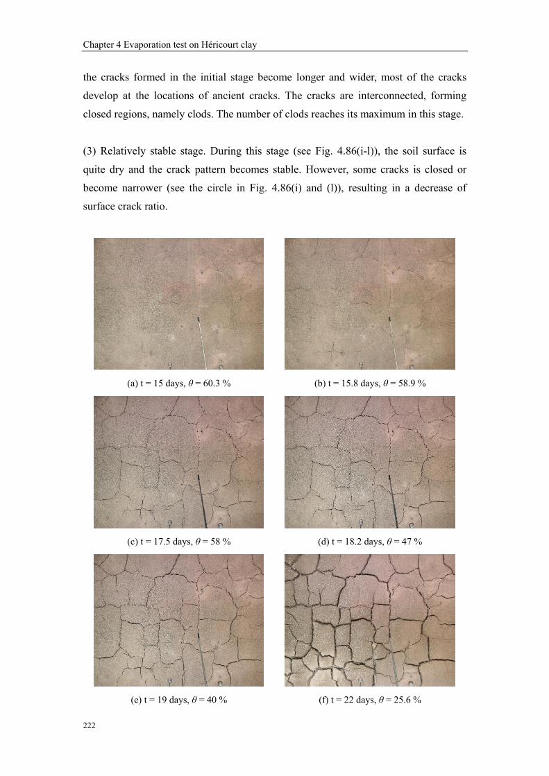
Chapter 4 Evaporation test on Héricourt clay
222
the cracks formed in the initial stage become longer and wider, most of the cracks
develop at the locations of ancient cracks. The cracks are interconnected, forming
closed regions, namely clods. The number of clods reaches its maximum in this stage.
(3) Relatively stable stage. During this stage (see Fig. 4.86(i-l)), the soil surface is
quite dry and the crack pattern becomes stable. However, some cracks is closed or
become narrower (see the circle in Fig. 4.86(i) and (l)), resulting in a decrease of
surface crack ratio.
(a) t = 15 days, θ = 60.3 %
(b) t = 15.8 days, θ = 58.9 %
(c) t = 17.5 days, θ = 58 %
(d) t = 18.2 days, θ = 47 %
(e) t = 19 days, θ = 40 %
(f) t = 22 days, θ = 25.6 %

Chapter 4 Evaporation test on Héricourt clay
223
(g) t = 24.2 days, θ = 21.8 %
(h) t = 26 days, θ = 20.2 %
(i) t = 28 days, θ = 17.46 %
(j) t = 36 days, θ = 7.9 %
(k) t = 42 days, θ = 6.2 %
(l) t = 54 days, θ = 4.2 %
Fig. 4.86. Propagation of crack pattern upon soil water evaporation (θ is the volumetric water content at 25-mm depth)

Chapter 4 Evaporation test on Héricourt clay
224
0 5 10 15 20 25 30 35 400
40
80
120
160
200 Edge Center
Dep
th (m
m)
Width (mm)
y=10x
y=1.14x
Fig. 4. 87. Depth versus width of cracks
Direct measurements of depth and width of cracks were carried out using a ruler and
are presented in Fig. 4.87. It is observed that the largest crack of 33 mm is in the
central part of the soil surface, while the deepest crack of 132 mm is at the center and
at the edges. Moreover, at the edges, cracks show limited width variations (10-17 mm)
but significant depth variations (70-130 mm). The limited width reflects the influence
of the chamber wall. There is no clear relationship between the depth and the width,
their ratio varying from 1.14 to 10.
4.4 Discussions
4.4.1 Evolution of soil parameters during infiltration
The evolution of volumetric water content shows that the increase of volumetric water
content in deep zone is earlier than that in shallow zone and the increase rate also
show the same manner (Fig. 4.15). This phenomenon is consistent with the water
transfer trend: as the water enters the chamber from the bottom, the water transfer in
the soil is driven by the effect of suction from the bottom to the surface. The opposite
phenomenon was observed when infiltration was processed from the surface (e.g.,
Tang et al., 2009; Ta, 2009). At the end of infiltration, the volumetric water content
decrease over depth but all the values are higher than the saturated one (48.1 %)
deduced from the initial dry density and the specific gravity. This can be attributed to
the swelling of soil during infiltration, the swelling of the upper layer being larger

Chapter 4 Evaporation test on Héricourt clay
225
than that of the lower layer. As the swelling corresponds to a decrease in dry density,
an increase in volumetric water content at saturated state is produced. Similar
phenomenon was observed by Tang et al. (2009) and Ta (2009) in a large-scale
infiltration test.
The uniform distribution of the initial volumetric water content suggests that the
applied compaction procedure allows a homogeneous sample to be prepared. The
similar values of volumetric water content in the zone below the 55-mm depth at the
beginning and the end of infiltration also confirm the homogeneity of the sample in
terms of density and water content (Tang et al., 2009).
For the relative humidity (Fig. 4.17), at the initiation of infiltration, the values are
nearly the same over the whole depth, also suggesting the homogeneity of the soil
sample. During infiltration, its evolution is similar to that of volumetric water content:
the larger the distance from the wetting end, the later the increase of relative humidity.
Furthermore, the increase rate of relative humidity decreases with the increase of
distance from the soil bottom. This was also observed in an infiltration test on
compacted sand-bentonite mixture under constant-volume and free-swell conditions
conducted by Cui et al. (2008) and in an infiltration test on the confined compacted
GMZ bentonite performed by Ye et al. (2009). Furthermore, this pattern is also similar
to the evolution of volumetric water content observed by Lemaire et al. (2004).
Clayey soil swells once in contact with water. As can be seen in Fig. 4.24, during
infiltration a large amount of swell is identified. The infiltration from the soil bottom
induces a sharp surface heave, and the heave rate decreases gradually over time. This
phenomenon was also observed in laboratory tests conducted by Abduljauwad et al.
(1998), Kim et al. (1999), Tang et al. (2009) and Ta (2009). Furthermore, when water
enters the soil column from the surface, a rapid heave in a short time is identified,
followed by a stabilization. This is consistent with the observation by Tang et al.
(2009) and Ta (2009).
Two boundary effects can be observed during infiltration (Figs. 4.22, 4.23 and 4.25):
limiting the soil surface heave at boundary and affecting the soil temperature. As can
be seen in Fig. 4.25, the heave at the central part of the surface is much higher than
that at the four edges, suggesting a significant effect of the friction existing between

Chapter 4 Evaporation test on Héricourt clay
226
the chamber wall and the soil. On the other hand, as can be seen in Figs. 4.22 and 4.23,
the evolution of soil temperature measured by PT1000 that was buried in the soil
shows less variation than those measured by T3111 transmitter that was installed on
the chamber wall, indicating a boundary effect on soil temperature.
4.4.2 Evolutions of soil and air parameters during evaporation
The free water evaporation is mainly affected by the atmospheric parameters. The
evaporation rate increases with increasing air temperature (Fig. 4.50) and wind speed
(Fig. 4.51). Similar phenomenon was observed by Kondo et al. (1992) through
numerical simulation, by Yamanaka et al. (1997) and Wang (2006) through laboratory
test in wind tunnel, and by Ta (2009) through an environmental chamber test. It is
worth noting that the evaporation rate of free water can also be considered as the
potential evaporation rate occurring in the constant-rate stage of soil water
evaporation process. As reported by Hillel (2004), one of the requirements for the
evaporation initiation is the existence of a vapor pressure gradient between the
evaporating surface and the atmosphere; in addition, the vapor should be transported
away. This explains why the increasing wind speed can accelerate the transportation
of vapor and hence increases the evaporation rate. Wang (2006) also reported that the
wind can quickly transport the water vapor to the atmosphere, thus increasing the
evaporation rate. In terms of resistance to evaporation (Kondo et al., 1992), the
evaporation rate during free water evaporation or that the constant-rate evaporation
stage for wet soils is almost governed by the aerodynamic resistance. The
aerodynamic resistance is sensitive to wind speed and hence wind speed significantly
affects the evaporation rate.
When increasing the heating tube temperature, an increase in the air temperature at
inlet is produced and thereby an increase in the chamber (Fig. 4.43), resulting in an
increase of energy for evaporation. As a result, the evaporation rate increases with
increasing air temperature at inlet (Fig. 4.50). Note that the significant effect of
atmospheric parameters on the evaporation rate is also observed in the
constant-evaporation rate stage for sand (see Chapter 3), confirming that the potential
evaporation is governed by the atmospheric parameters.

Chapter 4 Evaporation test on Héricourt clay
227
During free water evaporation, the air temperature at inlet also has significant
influence on the air temperature in the chamber. The evolutions of air temperature at
different elevations show similar manner to that at inlet, as well as at outlet (see Figs.
4.42 and 4.43). When the evaporation test is conducted at constant air heating tube
temperature (50 °C), the increase of air flow rate decreases the temperature at inlet
and hence the energy supplied to air in the chamber is decreased. However, when the
evaporation test is performed with increasing heating rube temperature, more energy
can be supplied to the air inside the chamber, resulting in an increase of the
temperature in the chamber. Similar result was obtained in the sand evaporation test
under high heating temperatures (see Chapter 3).
Both the air and soil temperatures were affected by the energy transformation during
evaporation (see Figs. 4.43 and 4.44). The water evaporation process consumes
energy and results in a decrease of temperature of the surrounding materials. A higher
evaporation rate requires more energy, and hence resulting in a larger temperature
decrease. When the water evaporation test is conducted at increasing air flow rate, the
evaporation rate is also increased (Fig. 4.48). Therefore, the temperatures of air, water
surface and soil decrease accordingly during this process. This phenomenon was also
observed during the initiation of sand evaporation at low heating temperature in this
study and by Wilson et al. (1994) in a column drying test.
Once the water evaporation is conducted at increasing heating temperature, the hot air
can supply more energy, and the energy from the hot air can be absorbed by air, water
layer and soil and hence increasing their temperatures on one hand, and being used for
water evaporation on the other hand. As a result, the temperatures of soil and air are
increased, as well as the evaporation rate. Similar result was observed in the sand
water evaporation test at high heating tube temperatures (see Chapter 3).
For the air-soil temperature profiles (Fig. 4.45), when water evaporates with
increasing air flow rate, the lowest temperature is located at the water surface and two
temperature gradients at water surface are identified: temperature decreases from the
50-mm height to the water surface; temperature increases from water surface to the
50-mm depth. Due to the low temperature at inlet, the energy used for water
evaporation is mainly from water and soil and hence their temperatures decrease.

Chapter 4 Evaporation test on Héricourt clay
228
Therefore, the lowest temperature appears at the evaporating surface, i.e., water
surface. By contrast, when evaporation is conducted with increasing heating
temperature, the energy from the hot air is enough for water evaporation. Therefore,
part of the energy is used for evaporation and the rest for heating the air, water and
soil. Similar evolutions of air-soil temperature profiles were identified by Ta (2009).
For the relative humidity, it decreases during the evaporation process (Fig. 4.46).
When the air flow rate is increased, the water vapor transported from the chamber
increases in rate, resulting in a decrease of the air relative humidity in the chamber.
When the air temperature is increased, the saturated vapor pressure increases and
more water vapor can be absorbed by air, thus decreasing the relative humidity inside
the chamber.
As far as the changes of atmospheric parameters during the two soil water evaporation
tests are concerned, they are very close. The air flow rate is 155 ± 5 L/min in the first
evaporation test (Test 1) (Fig. 4.26) and it shows a little decrease (140 ± 5 L/min) in
the second evaporation test (Test 2) (Fig. 4.52). The wind speeds at 50-mm above the
soil surface in Test 1 and Test 2 are 0.4 m/s and 0.36 m/s (Figs. 4.27 and 4.53),
respectively. The air temperature at inlet in Test 1 is as high as 56 ± 4 °C (Fig. 4.28)
and results in a variation of air temperature from 22 °C to 32 °C in the chamber (Fig.
4.29). Similarly, the air temperature at inlet in Test 2 is 55 ± 4 °C (Fig. 4.54) and
induces a temperature variation between 23 °C and 33 °C (Fig. 4.55). For the air
relative humidity, it decreases from 55 % to 11 % in Test 1 (Fig. 4.32) and from 44 %
and 14.8 % in Test 2 (Fig. 4.58). Furthermore, the evolution of relative humidity
shows a similar manner as the evaporation rate.
For the evolution of air-soil temperature profiles (Figs. 4.31 and 4.57), a clear
temperature decrease is observed at three locations: 50-mm height, soil surface and
50-mm depth. This was also observed in the sand evaporation test in the case of high
heating temperature. In general, the soil temperature increases as the increase of air
temperature, suggesting that the energy for evaporation is from hot air and that part of
the energy is used for heating soil and air. The decrease of temperature gradient
between 50-mm height and soil surface is attributed to the increasing energy used for
heating soil and air when the evaporation rate decreases. Furthermore, the enlarged

Chapter 4 Evaporation test on Héricourt clay
229
temperature gradient between the soil surface and the 50-mm depth suggests a
deepening of the drying front, as observed in the sand evaporation test. For the soil
temperature evolution, the change of soil temperature with air temperature changes is
found larger in clay than in sand. This phenomenon may be attributed to the effect of
cracks: cracks make the evaporation change from a one-dimension process to a
three-dimension process, allowing the air condition to affect the soil temperature in
deeper zones.
For the evolution of volumetric water content (Figs. 4.33 and 4.59), the dense
installation of sensors in the near surface zone allows the good monitoring of
volumetric water content in this zone, avoiding determining water content by
oven-drying method (e.g., Ta, 2009). In general, the surface soil layer loses water
firstly and the deeper zone starts to lose water only by the end of test. Similar results
were obtained in the sand evaporation test (see Chapter 3). Comparison between the
case of Fontainebleau sand and the case of Héricourt clay shows that the scenarios are
quite different: for the clay, only the water content at the 25-mm depth decreases
quickly at the initiation of evaporation, and then at deeper locations. However, for
sand, the entire zone from the surface to the 55-mm depth loses water quickly. This
can be attributed to the higher water retention capacity in the Héricourt clay and to the
effect of cracks.
Regarding the water content profiles (Figs. 4.34 and 4.60), the change of profile in the
zone from the surface to the 55-mm depth at t = 12 days in Test 1 and after t = 16 days
in Test 2 indicates a rapid decrease of water content and suggests a possible transition
of evaporation mode from one-dimensional to three-dimensional. Similar
phenomenon was observed by Konrad and Ayad (1997) in a field experiment.
Furthermore, similar evolution of water content profile was also observed in their
study. A linear relationship between water content and depth is observed in the near
surface zone, and this linear relationship extends to deeper zone as also observed in
the sand evaporation test. This linear relationship was also observed by Ta (2009)
through measuring the water content by oven-drying.
For the evolution of evaporation rate in the two tests (Figs. 4.38 and 4.64), the value
in the constant-rate stage is nearly the same while the duration of this stage in Test 1 is

Chapter 4 Evaporation test on Héricourt clay
230
longer than in Test 2. This can be attributed to the effect of the evolution of cracks in
this stage: more cracks appear in Test 2 and hence more water is evaporated in this
case.
4.4.3 The initiation of soil cracks
In general, the desiccation cracks are induced by water evaporation from the soil
surface (Inci, 2008). The desiccation cracking behavior depends on many factors such
as clay mineralogy, clay fraction, compaction conditions, layer thickness and size,
boundary conditions, wetting-drying cycles, drying process, soil particle orientation,
etc. (Fang, 1997; Nahlawi and Kodikara, 2006; Inci, 2008; Tang et al. 2008b, 2010b).
It is common practice to use the tensile strength criterion to describe the initiation of
cracks - desiccation cracks occur when the tensile stress induced by evaporation
exceeds the tensile strength of soil (Costa et al., 2008). Indeed, when an initially
saturated soil is subjected to the evaporation process, capillary suction will be
produced in the surface layer of soil. Meanwhile, a tensile stress develops in soil, and
increases with the increase of capillary suction. Once its value exceeds the tensile
strength of soil at a given location, the desiccation crack appears. In this sense, Tang
et al. (2011b) considered that the soil suction and tensile strength are two main
parameters governing the initiation of desiccation cracks, and the soil suction is the
mechanical indicator of cracking.
As far as the compacted soil in the chamber is concerned, as locally it is
heterogeneous, the evaporation rate at a specific location and the development of
suction are not strictly uniform at the soil surface. Therefore, the development of
tensile stress is also not uniform. In this case, cracks occur in the location where the
tensile stress is larger than the corresponding tensile strength, with a random
distribution (see Fig. 4.75(b)). Generally, cracks occur first in the zone with defects
such as the zone with sensors buried and the zone where soil samples were taken for
additional analyses (Fig. 4.88). Note however that these cracks are very limited in
number and their effect on the global cracking behavior can be ignored.

Chapter 4 Evaporation test on Héricourt clay
231
(a) Taking soil sample
(b) Burying sensors
Fig. 4.88. Cracks initiating at surface defects
4.4.4 The critical water contents
Two important parameters introduced by Tang et al. (2010b, 2011a, 2011b) are
identified, i.e., initial critical water content and final critical water content. Note that
the two critical water contents were also used by Li and Zhang (2011) to identify the
stage of crack development. The initial critical water content indicates the water
content at which the first crack appears. Therefore, to some extent, this parameter is a
bridge between the evaporation process and the mechanical indicator (suction) of
cracking (Tang et al., 2011b). The initial critical water content values in the first and
second evaporation tests are 58.9 % and 60.3 %, respectively. They are much higher
than the saturated water content (48.1 %), indicating that the soil is saturated at the
time considered. Meanwhile, as can be seen in Figs. 4.74 and 4.85, the evaporation is
in the constant-rate stage when the first crack appears. Therefore, we can conclude
that the soil starts to crack in the constant-rate stage when the soil is still fully
saturated. This observation is in agreement with the results obtained by Tang et al.
from the desiccation tests on the Romainville clay slurry under different temperatures
(2010b) or upon wetting-drying cycles (2011a), and on the Xiashu clay slurry (2011b).
It is also consistent with the results from gels desiccation tests reported by Brinker
and Scherer (1990). It is worth noting that the initial critical water content is also
affected by the soil layer thickness (Nahlawi and Kodikara, 2006), relative humidity
conditions during evaporation (Rodríguez et al., 2007), environmental temperature
(Tang et al., 2010b) and wetting-drying cycles (Tang et al., 2011a). In this study, the
initial critical water content is a little higher in the second evaporation test than in the
first one, in agreement with the results obtained by Tang et al. (2011a).

Chapter 4 Evaporation test on Héricourt clay
232
For the final critical water content, it varies from 30 % (the first evaporation test) to
17.5% (the second evaporation test). When the water content is lower than the critical
one, the surface crack ratio usually shows a relative stable value. Thus, the final
critical water content can be considered as or close to the shrinkage limit. However,
the shrinkage limit obtained in the laboratory is 23.8 %. The difference is perhaps due
to the different methods used in determining the shrinkage limit (compacted soil in
this study but soil slurry in the laboratory test) on one hand, and the inaccurate
measurement of water content when the sensor is exposed to the atmosphere due to
soil cracking on the other hand.
4.4.5 The three stages of crack evolution
Similar to the evolution of the actual evaporation rate, the evolution of crack can be
divided into three stages (Figs. 4.75 and 4.86): (1) initial stage; (2) quick development
stage and (3) relatively stable stage. As can be seen in the related photographs (Figs.
4.75 and 4.86), during initial stage only few cracks appear at different locations of soil
surface where the tensile stress exceeds the soil tensile strength. The surface crack
ratio in this stage is lower (Figs. 4.66 and 4.77) and the evaporation rate is quite high
(constant-rate stage). In the quick development stage, cracks develop quickly in
length, in width and also in depth. The gradual increase of cracks forms a polygonal
network on the soil surface. In that case, water evaporates from soil in a
three-dimensional manner: water vapor leaves from soil surface and from the wall of
crack simultaneously, accelerating thereby the evaporation process and resulting in a
rapid decrease of volumetric water content in soil, especially in the near surface zone.
As a result, the cracks become wider and deeper. During the relatively stable stage,
the crack pattern is stable but some cracks are gradually closed. This stage appears
after the water content is lower than the final critical water content. As can be
observed in Figs. 4.68 and 4.79, the water content in this stage is close to the
shrinkage limit, the soil particles almost reach their densest configuration and the pore
volume remains stable with further water loss (Krisdani et al., 2008; Tang et al.,
2010b). Therefore, the cracks’ propagation also trends to end after this critical water
content. However, the evaporation in cracked soil is still a three-dimensional process.
The water content in deeper zones is still higher than the shrinkage limit and the water
loss will still induce soil mass shrinkage. Therefore, the surface soil with stable cracks
will move due to the shrinkage of deeper soil mass. On the other hand, the shrinkage

Chapter 4 Evaporation test on Héricourt clay
233
of deeper soil is different due to the various crack depths; therefore, some cracks may
be closed. As the total soil mass is shrinking during evaporation, the boundary
shrinkage ratio increases (Figs. 4.67 and 4.78). Therefore, the shrinkage of the whole
soil mass leads the soil to move to the central position, closing thereby some cracks.
This phenomenon is also observed by Zhang et al. (2011), and they attribute it to the
change of water content gradient, the spatial distribution of dehydration rate and the
shrinkage at the bottom. Based on the field observation, Li and Zhang (2011) also
divided the soil cracking into three stages: initial stage; primary stage and steady stage.
However, the crack closure was not reported. It is possible that in field condition this
phenomenon is not pronounced due to the lack of boundary effects.
4.4.6 Changes of quantitative analysis parameters
The surface crack ratio changes with decreasing water content following four stages
(Figs. 4.68 and 4.79): slow increase before reaching the initial critical water content;
rapid increase in a narrow water content range; steady and decrease stage after the
final critical water content. The slow increase stage, rapid increase stage and the
subsequent steady stage are also observed by Tang et al. (2010b; 2011a; 2011b; 2011c)
in their laboratory experiments, but without the decrease stage. The surface crack ratio
decrease with water loss after a maximum value was reported by Zhang et al. (2011).
The major cause is the closure of cracks during this stage. Zhang et al. (2011) pointed
out that the water content at top soil is low in the later stage of evaporation; thus, the
water loss at soil bottom results in soil shrinkage, leading the stress state of the top
soil to change from tensile stress to compressive stress and closing thereby the crack
closes at some locations. The difference of the surface crack ratio during the last stage
of evaporation between different works can be due to: (1) the soil initial state: clay
slurry was used in the experiments conducted by Tang et al. (2010b; 2011a; 2011b;
2011c), while compacted soil was used in this study and in the experiment performed
by Zhang et al. (2011); (2) the thickness of soil layer: 8 mm and 10 mm thick soil
layer was studied by Tang et al. (2010b; 2011a; 2011b; 2011c), 20 mm soil thickness
was considered by Zhang et al. (2011) and 250 mm thick soil layer was used in this
study and (3) the base effect: the base restrains the movement of soil, while this effect
decreases as the soil thickness increases.
The surface crack ratio increases with increasing wetting-drying cycles. Indeed, the

Chapter 4 Evaporation test on Héricourt clay
234
surface crack ratio is higher in the second evaporation than in the first,
21.02 %-22.2 % against 17 %-19.28 %. This was also observed in a compacted clay
drying experiment conducted by Yesiller et al. (2000) and in a clay slurry desiccation
experiment performed by Tang et al. (2011a). The possible reason is that under the
effect of wetting-drying cycles, some irreversible fabric changes occurred in soil, and
thus decreasing the specimen integrity and increasing the weak zone in soil mass
(Yong and Wakentin, 1975; Tang et al., 2011a). The wetting-drying cycles leads the
tensile strength to decrease and the surface crack ratio to increase.
As can be seen in Figs. 4.70 and 4.81, the number of clods after the second
evaporation test is a little larger than after the first one. Generally, the soil subjected
to wetting-drying cycles generates weakened zones inside it, and can split into more
clods by cracks upon drying. The subsequent wetting process can heal the cracks
created (Yesiller et al., 2000; Li and Zhang, 2011). Therefore, the cracks developed in
the first drying process may not occur during the subsequent drying and thus the clods
number may not change. The photographs of cracked soil when the maximum clod
number confirm this reasoning (Fig. 4.89). In this figure, the zones covered by black
circles represent the soil subjected to cracking while the white ones show the healed
soil.
(a) The first evaporation test
(b) The second evaporation test
Fig. 4.89. Photographs of cracked soil
Based on the crack parameters shown in Figs. 4.68-4.73 and 4.79-4.84, it can be
observed that the number of clods, the number of nodes and crack segments, the
average length and width of crack segment and the crack length and number of crack
segments per unit area show similar evolution trend, all these parameters reach a
relative stable stage after the critical water content. Furthermore, similar evolution

Chapter 4 Evaporation test on Héricourt clay
235
was also observed for the development of surface crack ratio with decreasing
volumetric water content. As the surface crack ratio represents the desiccation
cracking, it is not necessarily related to the number of cracks. Therefore, the surface
crack ratio can be considered as the major parameter in the analysis of evaporation
process.
As far as the evolution of actual evaporation rate and the surface crack ratio during
evaporation are concerned, it is observed that the surface crack ratio increases slowly
in the constant-rate evaporation stage, and then it increases sharply during the later
constant-rate and the falling-rate stage evaporation. Finally, it shows a relatively
stable state during the later falling-rate stage and the slow-rate stage evaporation. As
the constant-rate stage evaporation is controlled by the atmospheric conditions, the
appearance of a few cracks has less influence on the actual evaporation rate. However,
once a large number of cracks appear (rapid increase stage), water evaporates to the
atmosphere in three-dimensional manner and water loss is enhanced.
A decrease of water content usually results in an increase in suction and hence a
decrease of evaporation rate. After the later falling-rate stage and during the slow-rate
stage, an equilibrium of water vapor exchange between soil and atmosphere is
reached, leading to a steady state for both the evaporation and the soil cracking. As
reported by Li and Zhang (2011), the steady state means very slow development of
cracks. As can be seen in Figs. 4.74 and 4.85, during the constant-rate evaporation
stage, the surface crack ratio after the second evaporation test is much larger than after
the first one. Furthermore, the period of constant-rate stage in the second evaporation
test is shorter than in the first one. Thus, we can conclude that the surface cracking
has significant influence on the constant-rate stage for water evaporation. Tang et al.
(2011b; 2011c) reported that most cracks (90 %) are developed in the constant-rate
stage. However, only 33-60 % of the whole cracks develop during this stage in our
study. This difference may be due to the soil thickness. The thin layer considered by
Tang et al. (2011b; 2011c) cannot have enough water for evaporation, and hence has a
large water content gradient over the soil thickness, accelerating the desiccation
process. On the other hand, a smaller gradient exists in our thicker layer and the
desiccation process is relatively reduced.

Chapter 4 Evaporation test on Héricourt clay
236
4.4.7 Evolution of crack pattern
Comparison among the cracked soil photographs, at the initiation stage, at the end of
the first and second evaporation tests (Figs. 4.75 and 4.86) shows that the cracks in
the second evaporation test appear at nearly the same locations as the first one. This
confirms the observations by Yesiller et al. (2000) on a compacted clayey soil, by
Tang et al. (2008b) on clayey soil slurry, and by Li and Zhang (2011) on a compacted
soil ground and an excavated soil surface in field conditions. This can be explained by
the fact that the cracks appeared after the first evaporation process represent weak
zones with lower tensile strength after being healed by the subsequent wetting.
As can be observed from the photographs of crack propagation (Figs. 4.75 and 4.86),
during the first evaporation test, a few small cracks appear in the weak zone of soil
surface; then some cracks become interconnected, resulting in the decrease of crack
segments number and hence the change in average length (Figs. 4.71 and 4.72). After
that, the crack propagation enters the quick development stage. Some large cracks are
formed in this stage, and the cracks tend to be intersected and form an interconnected
polygon network (Fig. 4.75(e-h)). During this stage, the propagation of cracks is as
follows: (1) short cracks gradually interconnect and form a long crack; (2) new cracks
develop from the existing cracks in the perpendicular direction (Fig. 4.90(a)); (3) the
propagating cracks tend to develop toward the existing crack at right angles (Fig. 4.90
(b)). Meanwhile, some cracks stop during propagation and form dead-end cracks.
Furthermore, the crack intersections usually form regular “T” shapes and a small
number of “+” shapes. The same observation was made by Tang et al. (2008b; 2011b;
2011c). Tang et al. (2011b; 2011c) interpreted this phenomenon based on the
maximum stress release criterion and the crack propagation criterion (Lachenbruch,
1962; Morris et al., 1992): cracks usually grow in the direction normal to the local
maximum tensile stress. In the existing cracks, the tensile stress perpendicular to it
has been released, and thus the new direction of the maximum tensile stress must be
parallel to the existing cracks. As a result, the initial direction of the new cracks that
start from the existing cracks will be perpendicular to them. For the propagating crack,
its development direction will progressively turn toward the preexisting cracks until
they intersect at right angles. During the last stage of crack propagation, the crack
pattern is nearly unchanged, except the change in width. As far as the crack
propagation in the second evaporation test is concerned, it is observed that the cracks

Chapter 4 Evaporation test on Héricourt clay
237
initiate at the same locations as in the first evaporation process, and the crack pattern
is also similar, showing that the cracks formed in the first evaporation process become
the weak zones with lower tensile strength, and can open again in the subsequent
evaporation test. Furthermore, this result also presents that the effect of
wetting-drying cycle on the evolution of desiccation cracking pattern is not obvious in
this study, this probably due to the limited cycles.
The crack pattern in this study is not as smooth and regular as that observed by Tang
et al. (2008b; 2010b; 2011a; 2011b; 2011c), but similar to that observed in field by Li
and Zhang (2011) and Konrad and Ayad (1997), and in the laboratory by Yesiller et al.
(2000). This may be explained by the difference in soil state (compacted soil, slurry
soil, intact soil) and in sample thickness.
(a)
(b)
Fig. 4.90. Crack propagation manner: (a) new cracks start from existing cracks; (b) crack develops perpendicularly to existing cracks

Chapter 4 Evaporation test on Héricourt clay
238
4.5 Conclusions
4.5.1 Infiltration test
The results obtained show that the evolution of volumetric water content can be
divided into three stages: (1) gradual increase at different depths, (2) sharp increase in
the surface 80-mm depth zone and (3) stabilization stage. In the first stage, the
increase of volumetric water in deep zones is earlier than that in shallow zones and
the increase rate also shows the same trend. This is related to the infiltration from the
bottom of soil. Furthermore, the uniform distribution of the initial volumetric water
content indicates the homogeneity of soil and confirms the compaction procedure
adopted. The much higher volumetric water content at the end of test is due to the soil
swelling.
As for the evolution of volumetric water content, the larger the distance from the
wetting end the later the increase of relative humidity. On the other hand, the increase
rate of relative humidity decreases with the increase of distance from the soil bottom.
During infiltration a large swell is observed on the soil surface. The infiltration from
the soil bottom induces a sharp increase of surface heave, and the increase rate
gradually slow down over time. Furthermore, once water enters the soil from soil
surface, a rapid heave is also observed in a short time, followed by a stabilization.
Two boundary effects are identified: reducing the soil surface heave at boundary and
affecting the soil temperature. The heave at the central part of the soil surface is much
larger than that at the four edges, suggesting a large fraction existing between the
chamber wall and the soil. The evolution of soil temperature measured by PT1000
that was buried in the soil shows fewer variations than that measured by T3111
transmitter that was installed on the wall of the chamber, indicating a boundary effect
on the soil temperature captured by T3111 transmitter.
4.5.2 Soil water evaporation test
4.5.2.1 Free water evaporation
The free water evaporation is mainly affected by the atmospheric parameters. The

Chapter 4 Evaporation test on Héricourt clay
239
evaporation rate increases with the increasing air temperature and wind speed. The
increasing wind speed can accelerate the transportation of water vapor, increasing
thereby the evaporation rate. Furthermore, the evaporation rate from free water is
governed by the aerodynamic resistance. As the aerodynamic resistance is sensitive to
wind speed, and the wind speed significantly affects the evaporation rate. Increasing
air temperature results in an increase of energy for evaporation.
During the free water evaporation, the air temperature at inlet has significant
influence on the air temperature in the chamber. The evolution of air temperature at
different elevations shows similar manner as those at inlet.
Both the air and soil temperatures are affected by the energy transformation during
evaporation. When water evaporation is processed at increasing air flow rate, the
evaporation process consumes energy from air, water layer and soil. Hence, the
temperatures of air, water surface and soil decrease with the increasing evaporation
rate. On the contrary, when water evaporation is processed at increasing heating
temperature, part of the energy from hot air can be used to heat air, water layer and
soil. Therefore, their temperatures increase along with the increase of evaporation
rate.
For the air-soil temperature profiles, when water evaporates with increasing air flow
rate, the lowest temperature is located at the water surface, and two temperature
gradients at water surface are identified: the temperature decreases from the 50-mm
height to the water surface; the temperature increases from the water surface to the
50-mm depth. By contrast, when evaporation is processed with increasing heating
temperature, only one temperature gradient is observed.
The relative humidity inside the chamber decreases with the increases of air flow rate
and heating tube temperature.
4.5.2.2 Soil water evaporation
The atmospheric parameters during the two soil water evaporation tests being similar,
the soil behavior in the two drying tests can be compared.
The air temperature at different heights in the chamber varies according to the

Chapter 4 Evaporation test on Héricourt clay
240
evolution of the temperature at inlet. This was also observed during the test on sand
(see Chapter 3).
The soil temperature is strongly affected by the air conditions, evaporation process
and desiccation cracking. The evaporation rate decreases with increasing soil
resistance due to the increase of soil suction, and thus more energy is available for
heating soil. The cracks increase the evaporating surface and hence enhance the
influence of air condition on the soil temperature.
For the air-soil temperature profiles, an obvious temperature decrease is observed at
three locations: 50-mm height, soil surface and 50-mm depth. The soil temperature
increases with the increase of air temperature, suggesting that the energy for
evaporation is from hot air, and that part of the energy is used for heating soil and air.
The decrease of temperature gradient between the 50-mm height and the soil surface
is attributed to the increasing energy used for heating soil and air along with the
decreasing evaporation rate. The enlarged temperature gradient between the soil
surface and the 50-mm depth suggests a deepening of the drying front.
The air relative humidity decreases with the decreasing evaporation rate. Three stages
are identified: (1) a decrease at a quite low rate; (2) a sharp decline stage; (3) a slow
decrease followed by a stabilization. Note also that the variations of relative humidity
in the laboratory do not affect the values in the chamber.
For the volumetric water content, the dense installation of sensors in the near surface
zone allows a continuous measurement in this zone, avoiding determining the water
content by oven-drying. The surface soil layer loses water firstly and the deeper zone
starts to lose water by the end of test. The evolution of volumetric water content in the
near surface zone is quite different from that for the Fontainebleau sand: for the
Héricourt clay, the water content decreases quickly only at the 25-mm depth in the
beginning, and then at deeper locations. However, for the Fontainebleau sand, the
entire zone in the zone from the surface to the 55-mm depth loses water quickly at the
same time. This can be attributed to the higher water retention capacity in clayey soils
like the Héricourt clay and to the effect of cracks.

Chapter 4 Evaporation test on Héricourt clay
241
Regarding the water content profiles, the rapid change during the early stage of
evaporation in zone from the surface to the 55-mm depth suggests a rapid decrease of
water content and a possible transition of evaporation mode from one-dimensional to
three-dimensional. The linear relationship between water content and depth appears in
the surface zone, and this relationship was also observed by Ta (2009) through
measuring water content by oven-drying. This linear relationship extends to deeper
zone as observed in the sand evaporation test. Furthermore, the large change of water
content in the surface zone suggests that evaporation mainly affect this zone. However,
the development of cracks toward deeper zone extends the influence zone of
evaporation.
The evolution of evaporation rate in the two tests shows three stages. The evaporation
in the constant-rate stage is nearly the same while the duration of this stage is longer
in Test 1. This can be attributed to the evolution of cracks, more cracks appear in Test
2 and hence more water is evaporated in this case.
4.5.3 Soil desiccation cracking
Cracks are initiated at the locations where the soil tensile stress is larger than its
corresponding tensile strength. The local heterogeneity of compacted soil results in a
non-uniform development of tensile stress at different locations, giving rise to a
random distribution of cracks.
The initial and final critical water contents are two important parameters for
describing the desiccation process. The initial critical water content corresponds to the
appearance of the first crack and is usually higher than the saturated water content. Its
value is found higher in the second evaporation test than in the first one. The final
critical water content corresponds to the end of crack propagation and is related to the
shrinkage limit of soil. Once the water content is lower than this value, the
development of crack enters a relatively stable stage.
The development of surface crack ratio can be divided into four stages in different
evaporation tests. For the first evaporation test, the evolution of surface crack ratio is
as follows: (1) slow increase stage; (2) rapid increase stage; (3) slow decrease stage;
and (4) steady stage. For the second evaporation test, the evolution of surface crack

Chapter 4 Evaporation test on Héricourt clay
242
ratio is presented as follows: (1) slow increase stage; (2) rapid increase stage; (3)
steady stage; and (4) slow decrease stage. The surface crack ratio starts to increase
slowly after the initial critical water content is reached, and then it increases quickly
with the decreasing water content. After the final critical water content, it shows a
relative stable trend but with a little decrease due to the closure of cracks at some
locations. The surface crack ratio increases with increasing wetting-drying cycles.
Soil desiccation cracking starts during the constant-rate stage of evaporation when the
soil is still fully saturated. The surface crack ratio increases slowly in the constant-rate
evaporation stage, and then sharply during the later constant-rate and the falling-rate
evaporation stages. Finally, it shows a relative stable state during the later falling-rate
stage and slow-rate stage of evaporation. Notably, only 33-60 % of the whole cracks
take place during the constant-rate stage. This phenomenon is believed to depend on
the soil thickness. In addition, the duration of the constant-rate stage in the second
evaporation test is shorter than in the first one, suggesting that the surface cracks have
significant influence on the constant-rate stage.
Similar to the evolution of actual evaporation, the evolution of cracks can be divided
into three stages: (1) initial stage; (2) quick development stage; (3) relatively stable
stage. The propagation of cracks at different stages shows some clear trends: in the
first evaporation test, a few small cracks appear in the weak zone of soil surface in the
initial stage of crack propagation; then some cracks are interconnected, resulting in a
decrease of crack segments number and hence a change of average length. During the
quick development stage, the propagation of cracks is as follows: (1) short cracks
gradually meet to form a long crack; (2) new cracks develop from the existing cracks
in the perpendicular direction; (3) propagating cracks tend to develop toward the
existing cracks at right angles; (4) some cracks stop during propagation and form
dead-end cracks. Furthermore, the crack intersections usually have regular “T” shapes
and a small number of “+” shapes. During the last stage of crack propagation, the
crack pattern is nearly unchanged, except the change in width.
As far as the crack propagation in the second evaporation test is concerned, cracks
initiate at the nearly same locations as in the first evaporation test due to the weak
zones formed by drying and healed by the subsequent wetting, and the crack

Chapter 4 Evaporation test on Héricourt clay
243
propagation seems to be the extension of that in the first evaporation test, a few new
crack are observed. The closure of some cracks is attributed to the shrinkage of deeper
soil and of the whole soil mass.
The number of clods after the second evaporation test is a little larger than after the
first one, suggesting that some cracks developed in the first drying test are closed
during the subsequent drying.
The quantitative analysis parameters such as the number of clods, the number of
nodes and crack segments, the average length and width of crack segment and the
crack length and number of crack segments per unit area show similar evolution trend
as the development of surface crack ratio - reaching a relative stable stage after the
final critical water content by the end of evaporation test. Therefore, the surface crack
ratio can be considered as the major parameter in describing the evaporation process.

Chapter 4 Evaporation test on Héricourt clay
244

Chapter 5 Modelling of potential water evaporation
245
Chapter 5 Modelling of potential water evaporation
5.1 Introduction
As discussed in Chapter 1, modeling the actual evaporation usually needs the
knowledge of the potential evaporation rate. Thereby, an accurate determination of the
potential evaporation corresponds to an important prerequisite for determining the
actual evaporation.
As presented in Chapter 1, the mass transfer model is an attractive model for
predicting free water or wet soil evaporation (potential evaporation), because it has
many advantages compared to other models (Sign and Xu, 1997): (1) the form is
simple; (2) the related parameters are easy to be determined; (3) it covers the most
important meteorological factors affecting the potential evaporation such as vapour
pressure gradient, temperature and wind speed; (4) the prediction of evaporation rate
using this model has been found satisfactory. This explains its wide use over the world
and the large development of models based on its basis. Specifically, Sign and Xu
(1997) summarized 13 relatively simple and commonly used models, and reported
that the evaporation rate is proportional to the vapour gradient between the
evaporating surface and the air at a reference level and also proportional to the wind
speed at the reference level. However, the relationship between the evaporation rate
and temperature is not clear. Furthermore, based on the 13 different models, Sign and
Xu (1997) also proposed seven general forms of the existing models and verified
them using the meteorological data from different weather stations at different sites.
These generalized forms are beneficial for predicting the evaporation rate using data
from specific sites or experiments after calibration. Ta (2009) also proposed a two-
parameter model (wind speed and air relative humidity) for the prediction of potential
evaporation based on the data obtained from the tests using an environmental chamber
under different atmospheric conditions. Tran (2014) modified the model proposed by
Ta (2009) by introducing a logarithmic function instead of a linear function to
describe the wind speed effect.
In this study, the existing models will be assessed based on the data obtained and

Chapter 5 Modelling of potential water evaporation
246
presented in Chapter 4. A new model is then proposed and the related parameters will
be determined using the data from the test with free water evaporation. Finally, the
performance of the new model is verified based on the data from the sand and clay
evaporation tests.
5.2 Assessment of existing models
In this chapter, the assessed generalized forms of potential evaporation models are
listed in Table 5.1. The choice of these models is based on the fact that they allow
determination of the evaporation rate in a short term on one hand, and they represent
most of the popular models on the other hand. Furthermore, these models contain at
least two meteorological parameters such as temperature and wind speed. More
specifically, Models 1 to 6 correspond to the model proposed by Harbeck et al. (1954),
Horton (1919), Penman (1948) and Kuzmin (1957), Harbeck et al. (1958), and
Romanenko (1961), respectively.
Table 5.1 Generalized models (Singh and Xu, 1997; Ta, 2009; Tran, 2014)
Generalized models
Model 1 E = au (es-ea)
Model 2 E = a(1-exp(-u))(es-ea)
Model 3 E = a(1+bu)(es-ea)
Model 4 E = au(es-ea)(1-b(Ta-Ts))
Model 5 E = a(1+ bu)(es-ea)(1-c(Ta-Ts))
Model 6 E = a(Ta + 25)2 (100-ha)
Model 7 E = (a+bu)(100-ha)
Model 8 E = (a+blnu)(100-ha)
In Table 5.1, E is the potential evaporation rate (mm/day); es is the saturated vapor
pressure deduced by the water or soil surface temperature (Pa); ea is the air vapor
pressure deduced from the saturated vapor pressure determined by air temperature and
relative humidity (Pa); Ta is the air temperature (°C) at a reference height; Ts is the
surface temperature (°C); ha is the air relative humidity at the reference height (%); u
is the wind speed at the reference height (m/s). It is noted that the reference height is
50 mm above the soil (or water) surface in this study.

Chapter 5 Modelling of potential water evaporation
247
For each model, the related parameters are determined using the data from the free
water evaporation tests under different atmospheric conditions (different wind speeds
or air temperatures, see in Chapter 4). This process is conducted as follows: when the
undetermined parameters are related to wind speed, they will be determined using the
data obtained from the evaporation test with different wind speeds (i.e., free water
evaporation test presented in Chapter 4: Stage 1 to Stage 3); when the undetermined
parameters are related to temperature, they will be determined using the data obtained
from the evaporation test with different heating temperatures (i.e., free water
evaporation test presented in Chapter 4: Stage 4 to Stage 6). After the determination of
parameters, the models are also needed to be verified by experimental data. According
to the ways for the parameters’ determination, the verification of the models is
conducted in two different fashions: when the parameters in the model are determined
using the data obtained with different wind speeds, the models will be verified based
on the data obtained with different temperatures; reversed process will be followed in
the second case. Finally, the prediction results are compared with the experimental
results to verify the relevance of the models. The model with a good performance will
be selected as the potential evaporation model in this study. In case of no appropriate
model, a new model will be developed based on the existing models. In this case, the
proposed model will also be checked by the soil water evaporation results, as the
actual evaporation rate is supposed to be equal to the potential one at the constant-rate
stage.
5.3 Comparison between various models
5.3.1 Model 1
s a( )E au e e= − (5.1)
Only parameter a is needed to be determined in this model. Thus, from Equation 5.1,
we can obtain:
s a
Eaue e
=−
(5.2)
The data from the free water evaporation test with different wind speeds are used to
determine parameter a. For this purpose, the ratio of evaporation rate (E) to the vapor
pressure deficit (es-ea) with three different wind speeds was calculated and considered

Chapter 5 Modelling of potential water evaporation
248
as the value of au, and then a linear relationship between E/(es-ea) and u can be
observed in Fig. 5.1. Therefore, the parameter a can be determined: a = 0.014. After
that, the data from the evaporation experiment with different wind speed and heating
tube temperatures were used to verify Equation 5.1 with the determined parameter
(Fig. 5.2).
0.0 0.1 0.2 0.3 0.4 0.50.0
2.0x10⁻³
4.0x10⁻³
6.0x10⁻³
8.0x10⁻³E/
(es-e
a)
u (m/s)
y = 0.014xR2 = 0.905
Fig. 5.1. Relationship between E/(es-ea) and u
0 1 2 3 4 50
1
2
3
4
5
6
7
Pot
entia
l eva
pora
tion
rate
(mm
/day
)
Elapsed time (day)
Experiment Model 1
4 5 6 7 80
1
2
3
4
5
6
7
Pot
entia
l eva
pora
tion
rate
(mm
/day
)
Elapsed time (day)
Experiment Model 1
(a) (b)
Fig. 5.2. Verification of Model 1: (a) different wind speeds; (b) different heating tube temperatures
As can be seen in Fig. 5.2, the predicted and measured evaporation rates show the
same evolution trend: the evaporation rate increases with increasing wind speed and
heating tube temperature. Six different plateaus in this figure (3 in Fig. 5.2a and 3 in
Fig. 5.2b) correspond to different atmospheric conditions (constant wind speeds and
constant temperatures). The prediction value of the evaporation rate with increasing
wind speed agrees well with the measured one (Fig. 5.2(a)). However, the predicted
values are much higher than the measured ones in the case of increasing heating tube
temperature: the prediction value at 200 °C heating tube temperature (i.e. end of test)

Chapter 5 Modelling of potential water evaporation
249
is nearly three times higher than the measured one (Fig. 5.2(b)). This indicates that if
Model 1 is calibrated with wind speed, it cannot predict the evaporation correctly in
case of variable temperature.
5.3.2 Model 2
s a(1 exp( ))( )E a u e e= − − − (5.3)
In Equation 5.3, there is only one constant parameter a needing to be determined. For
its determination, Equation 5.3 is re-written as:
s a
(1 exp( )) = Ea ue e
− −−
(5.4)
Similar to the procedure adopted for Model 1, the experimental data from water
evaporation with different wind speeds are used to calculate the value of E/(es-ea).
Therefore, a nonlinear relationship between E/(es-ea) and u can be obtained and is
shown in Fig. 5.3. Therefore, parameter a can be determined from this relationship: a
= 0.017.
0.0 0.1 0.2 0.3 0.4 0.50.0
2.0x10⁻³
4.0x10⁻³
6.0x10⁻³
8.0x10⁻³
E/(e
s-ea)
u (m/s)
y = 0.017(1-exp(-x)) R2 = 0.95
Fig. 5.3. Relationship between E/(es-ea) and u
To verify this model, the values predicted by the model with the determined parameter
are compared with the experimental data obtained from the evaporation test with
different heating tube temperatures (Fig. 5.4(a)). Furthermore, for better describing
the wind speed effect, the predicted and measured values with different wind speeds
are also presented (Fig. 5.4(b)).

Chapter 5 Modelling of potential water evaporation
250
4 5 6 7 80
1
2
3
4
5
6
7
Pot
entia
l eva
pora
tion
rate
(mm
/day
)
Elapsed time (day)
Experiment Model 2
(a)
0 1 2 3 4 50
1
2
3
4
5
6
7
Pot
entia
l eva
pora
tion
rate
(mm
/day
)
Elapsed time (day)
Experiment Model 2
(b)
Fig. 5.4. Verification of Model 2: (a) different heating tube temperatures; (b) different wind speeds;
As can be seen in Fig. 5.4, the predicted results by Model 2 show similar trend to the
measured one. As for Model 1, Model 2 also gives consistent results for different
wind speeds (Fig. 5.4(b)). However, large deviation can be observed with increasing
heating temperature. The predicted value in this stage is 1.5-3 times larger than the
measured one (Fig. 5.4(a)).
5.3.3 Model 3
s a(1 )( )E a bu e e= + − (5.5)
In this model, there are two parameters a and b needing to be determined. For their
determination, Equation 5.5 is re-written as:
s
(1 )a
Ea bue e
+ =−
(5.6)
Thus, the value of a(1+bu) can be calculated based on the evaporation rate and vapor
pressure deficit (i.e., E/(es-ea)) during the evaporation test conducted with different
wind speeds: a linear relationship between u and E/(es-ea) can be observed in Fig. 5.5,
giving: a = 0.0007; b = 16.72.
To verify this model, the determined parameters are used to predict the evaporation
rate using the measured atmospheric data. Both the predicted and measured
evaporation rates are shown in Fig. 5.6. The predicted result is in agreement with the

Chapter 5 Modelling of potential water evaporation
251
experimental measurement in the case of different wind speeds (Fig. 5.6(a)). However,
for the evaporation test conducted with increasing heating temperature, the predicted
results are much larger than the measurement (Fig. 5.6(b)).
0.0 0.1 0.2 0.3 0.4 0.50.000
0.002
0.004
0.006
0.008
E/(e
s-ea)
u (m/s)
y = 0.0117x+0.0007 R2 = 0.943
Fig. 5.5. Relationship between E/(es-ea) and u
0 1 2 3 4 50
1
2
3
4
5
6
7
Pot
entia
l eva
pora
tion
rate
(mm
/day
)
Elapsed time (day)
Experiment Model 3
(a)
4 5 6 7 80
1
2
3
4
5
6
7
Pot
entia
l eva
pora
tion
rate
(mm
/day
)
Elapsed time (day)
Experiment Model 3
(b)
Fig. 5.6. Verification of Model 3: (a) different wind speeds; (b) different heating tube temperatures
5.3.4 Model 4
s a a s( )(1 ( ))E au e e b T T= − − − (5.7)
In this model, two constant parameters a and b need to be determined. For this
purpose, Equation 5.7 is re-written as:
a ss
a(1 b( ))( )a
ET Tu e e
− − =−
(5.8)
Thus, the right part of Equation 5.8 can be calculated by the data from the evaporation

Chapter 5 Modelling of potential water evaporation
252
tests with different heating temperatures (constant wind speed at 50 mm above the
soil surface). A linear relationship between E/u(es-ea) and Ta-Ts can be observed in Fig.
5.7, giving a = -0.0047 and b = 0.404.
4 5 6 7 8 90.000
0.002
0.004
0.006
0.008
0.010
0.012
0.014
Ta-Ts (°C)
y = 0.0019x-0.0047 R2 = 0.7206
Fig. 5.7. The relationship between E/u(es-ea) and Ta-Ts
After determining the related constant parameters in this model, it is verified using the
data from the evaporation test. As can be seen in Fig. 5.8, there is significant deviation
between the measured and predicted results. Therefore, even with a
temperature-related parameter, Model 4 is not able to predict the potential evaporation
rate satisfactorily.
0 1 2 3 4 5
0.0
0.5
1.0
1.5
2.0
2.5
3.0
Pot
entia
l eva
pora
tion
rate
(mm
/day
)
Elapsed time (day)
Experiment Model 4
(a)
4 5 6 7 80.0
0.5
1.0
1.5
2.0
2.5
3.0
Pot
entia
l eva
pora
tion
rate
(mm
/day
)
Elapsed time (day)
Experiment Model 4
(b)
Fig. 5.8. Verification of Model 4: (a) different wind speeds; (b) different heating tube temperatures
5.3.5 Model 5
s a a s(1 )( )(1 ( ))E a bu e e c T T= + − − − (5.9)
E/u(
e s-e
a)

Chapter 5 Modelling of potential water evaporation
253
In this model, three constant parameters (a, b and c) need to be determined. Equation
5.9 can be considered as the combination of Model 3 and 1-c(Ta-Ts). Therefore, by
letting parameters a and b equal to the values determined in Model 3, we obtain:
a s1- ( )=(1+ )( )s s
Ec T Ta bu e e
−−
(5.10)
Then, we determine the relationship between E/(a(1+bu)(es-ea)) and Ta-Ts (Fig. 5.9).
However, the linear relationship in this figure is in conflict with the expression
1-c(Ta-Ts). Indeed, a negative value of parameter c is obtained. To tackle this problem,
expression 1-c(Ta-Ts) is replaced by d+c(Ta-Ts) for describing the temperature
influence. Thereby, Equation 5.11 is obtained:
s a a s(1 )( )( ( ))E a bu e e d c T T= + − + − (5.11)
and a s0
+ ( )=(1+ )( )s
Ed c T Ta bu e e
−−
(5.12)
Using the relationship between Ta-Ts and E/(a(1+bu)(es-ea)) shown in Fig. 5.9.
Parameter c and d can be determined: c = 0.15; d = -0.36.
4 5 6 7 8 90.2
0.4
0.6
0.8
1.0
E/(a
(1+b
u)(e
s-ea))
Ta-Ts (°C)
y = 0.15x-0.36 R2 = 0.72
Fig. 5.9. Relationship between E/(a(1+bu)(es-ea)) and Ta-Ts
The model with the determined parameters is verified using the data from the water
evaporation test with different wind speeds and heating temperatures. As can be seen
in Fig. 5.10, the predicted results are smaller than the measured ones, and in addition,
different evolution trends are obtained. Therefore, Model 5 is not suitable for the
potential evaporation prediction.

Chapter 5 Modelling of potential water evaporation
254
0 1 2 3 4 50.0
0.5
1.0
1.5
2.0
2.5
3.0
3.5
Pot
entia
l eva
pora
tion
rate
(mm
/day
)
Elapsed time (day)
Experiment Model 5
(a)
4 5 6 7 80.0
0.5
1.0
1.5
2.0
2.5
3.0
3.5
Pot
entia
l eva
pora
tion
rate
(mm
/day
)
Elapsed time (day)
Experiment Model 5
(b)
Fig. 5.10. Verification of Model 5: (a) different wind speeds; (b) different heating tube temperatures
5.3.6 Model 6
2a a( 25) (100 )E a T h= + − (5.13)
For this model, there are two variables: air temperature and air relative humidity. Only
one constant parameter a is involved. For its determination, Equation 5.13 is
re-written as:
2( 25) (100 )a a
EaT h
=+ −
(5.14)
Then, the measured evaporation test data at constant wind speed with different air
temperatures are used to determine parameter a (Fig. 5.11). As can be observed in Fig.
5.12, the value of a fluctuates with changes of air temperature. An average value of
1.53×10⁻⁵ can be obtained.
4 5 6 7 81.0x10⁻⁵
1.5x10⁻⁵
2.0x10⁻⁵
2.5x10⁻⁵
a
Elspased time (day)
Fig. 5.11. Determination of parameter a

Chapter 5 Modelling of potential water evaporation
255
After the determination of parameter a, this model is verified using the experimental
data obtained from the evaporation test with different wind speeds (Fig. 5.12(a)). The
predicted results are also compared with the measured ones during the evaporation
test with different heating temperatures (Fig. 5.12(b)). As can be seen in Fig. 5.12, the
predicted results of Model 6 are consistent with the measured ones in case of
increasing heating temperature. However, significant difference is identified in case of
increasing wind speed.
0 1 2 3 4 50.0
0.5
1.0
1.5
2.0
2.5
Pot
entia
l eva
pora
tion
rate
(mm
/day
)
Elapsed time (day)
Experiment Model 6
(a)
4 5 6 7 80.0
0.5
1.0
1.5
2.0
2.5
Pot
entia
l eva
pora
tion
rate
(mm
/day
)
Elapsed time (day)
Experiment Model 6
(b)
Fig. 5.12. Verification of Model 6: (a) different wind speeds; (b) different heating tube temperatures
5.3.7 Model 7
a( )(100 )E a bu h= + − (5.15)
Model 7 is proposed by Ta (2009). In this model, the wind speed and air relative
humidity are considered. Two undetermined parameters related to wind speed (a and b)
are introduced. For their determination, Equation 5.15 is re-written as:
a100
Ea buh
+ =−
(5.16)
The data obtained from the water evaporation test with different wind speeds are used
to determine the right part of Equation 5.16. A linear relationship between E/(100-ha)
and u can be observed in Fig. 5.13, giving a = 0.022 and b = 0.031.

Chapter 5 Modelling of potential water evaporation
256
0.0 0.1 0.2 0.3 0.4 0.50.01
0.02
0.03
0.04
0.05
E/(1
00-h
a)
u (m/s)
y = 0.031x+0.022 R2= 0.52
Fig. 5.13. Relationship between E/(100-ha) and u
0 1 2 3 4 50.0
0.5
1.0
1.5
2.0
2.5
Pote
ntia
l eva
pora
tion
rate
(mm
/day
)
Elapsed time (day)
Experiment Model 7
(a)
4 5 6 7 80.0
0.5
1.0
1.5
2.0
2.5Po
tent
ial e
vapo
ratio
n ra
te (m
m/d
ay)
Elapsed time (day)
Experiment Model 7
(b)
Fig. 5.14. Verification of Model 7: (a) different wind speeds; (b) different heating tube temperatures
0.0 0.4 0.8 1.2 1.6 2.0 2.40.0
0.4
0.8
1.2
1.6
2.0
2.4
Mod
el p
redi
ctio
n (m
m/d
ay)
Experimental measurement (mm/day)
Fig. 5.15. Comparison between model prediction and experimental measurement

Chapter 5 Modelling of potential water evaporation
257
After determining the parameters, Model 7 is verified using the experimental results
obtained from the water evaporation test with increasing heating temperature. The
measured and calculated evaporation rates are shown in Fig. 5.14. As can be seen in
this figure, both the predicted and measured values are increasing with increasing
wind speed and heating temperature. The predicted values agree well with the
measured ones. The comparison between the model prediction and the experimental
measurement confirms this good agreement (Fig. 5.15). In conclusion, Model 7 is
reliable to predict the potential evaporation rate with varying atmospheric conditions.
5.3.8 Model 8
a( ln )(100 )E a u h= + − (5.17)
This model is proposed by Tran (2014). In this model, a nonlinear function with wind
speed replaces the linear function in Model 7. For determining the undetermined
parameters (a and b), the form of Equation 5.17 is changed to:
a
ln100
Ea u bh
+ =−
(5.18)
Furthermore, the right part of Equation 5.18 can be calculated using the data
measured during the evaporation test with different wind speeds. Therefore, the
relationship between E/(100-ha) and u can be obtained (Fig. 5.16), and parameters a
and b can be determined: a = 0.009; b = 0.043.
0.0 0.1 0.2 0.3 0.4 0.50.01
0.02
0.03
0.04
0.05
E/(1
00-h
a)
u (m/s)
y = 0.009lnx+0.043 R2 = 0.667
Fig. 5.16. The relationship between E/(100-ha) and u

Chapter 5 Modelling of potential water evaporation
258
0 1 2 3 4 50.0
0.5
1.0
1.5
2.0
2.5
Pote
ntia
l eva
pora
tion
rate
(mm
/day
)
Elapsed time (day)
Experiment Model 8
(a)
4 5 6 7 80.0
0.5
1.0
1.5
2.0
2.5
Pote
ntia
l eva
pora
tion
rate
(mm
/day
)
Elapsed time (day)
Experiment Model 8
(b)
Fig. 5.17. Verification of Model 8: (a) different wind speeds; (b) different heating tube temperatures
0.0 0.4 0.8 1.2 1.6 2.0 2.40.0
0.4
0.8
1.2
1.6
2.0
2.4
Mod
el p
redi
ctio
n (m
m/d
ay)
Experimental measurement (mm/day)
Fig. 5.18. Comparison between the model prediction and the experimental measurement
After determining the parameters, Model 8 is verified based on the experimental
results obtained from the water evaporation test with increasing heating temperature
and wind speed. The measured and calculated evaporation rates are shown in Fig.
5.17. As can be seen, the predicted values are consistent with the measured ones.
Comparison between the model prediction and the experimental measurement (Fig.
5.18) confirms this good agreement. In conclusion, Model 8 is also suitable for
predicting the potential evaporation rate with varying atmospheric conditions.
In reality, in the range of wind speed considered in the test (0 - 0.5 m/s), the effect of
wind speed is quite similar in Model 7 and Model 8. This explains the similar
prediction results by the two models.

Chapter 5 Modelling of potential water evaporation
259
5.3.9 Extended models
In this section, other combinations of wind, relative humidity and vapor pressure are
used for further analysis.
5.3.9.1 Modification of Model 3
As shown before, Model 3 gives a good prediction for different wind speeds, and in
Model 7 the form 100-ha indirectly reflects the temperature effect on evaporation
because ha is temperature dependent. Thus, we can propose a new model which
contains wind speed, vapor pressure and relative humidity as follows:
s a a(1 )( )(100 )E a bu e e h= + − − (5.19)
or
s a a
(1 b )( )(100 )
Ea ue e h
+ =− −
(5.20)
The right part of Equation 5.20 can be calculated using the data obtained from the
water evaporation test with different wind speeds: a linear relationship between
E/((es-ea)(100-ha)) and u can be obtained (Fig. 5.19), giving a = 0.00004 and b = 5.
After determining the related parameters, the modified Model 3 is verified by the
measured data. As can be seen in Fig. 5.20, the predicted result agrees well with the
experimental measurement in the first 4.7 days (i.e., evaporation with different wind
speeds) but it is 1.5-4 times larger than the measured value in the following time.
Therefore, this modified model is not suitable for the potential evaporation prediction.
0.0 0.1 0.2 0.3 0.4 0.50.0
4.0x10⁻⁵
8.0x10⁻⁵
1.2x10⁻⁴
1.6x10⁻⁴
E/((e
s-ea)(
100+
h a))
u (m/s)
y = 0.0002x+0.00004 R2 = 0.83
Fig. 5.19. Relationship between E/((es-ea)(100-ha)) and u

Chapter 5 Modelling of potential water evaporation
260
0 1 2 3 4 50
1
2
3
4
5
6
7
8
9P
oten
tial e
vapo
ratio
n ra
te (m
m/d
ay)
Elapsed time (day)
Experiment Modified Model 3
(a)
4 5 6 7 80
1
2
3
4
5
6
7
8
9
Pot
entia
l eva
pora
tion
rate
(mm
/day
)
Elapsed time (day)
Experiment Modified Model 3
(b)
Fig. 5.20. Verification of Modified Model 3: (a) different wind speeds; (b) different heating tube temperatures
5.3.9.2 Combination of Model 3 and Model 6
As discussed in Section 5.3, Model 3 is suitable for predicting evaporation rate with
different wind speeds but is not suitable for reflecting the temperature effect. By
contrast, Model 6 can give perfect prediction under increasing heating temperature
condition but poor prediction under different wind speeds condition. Thus, we can
propose a new model that combines these two models:
s a a a(1 )( )( 25) (100 )cE a bu e e T h= + − + − (5.21)
or
cs a a a
(1 )( )( 25) (100 )
Ea bue e T h
+ =− + −
(5.22)
According to Equation 5.22, parameters a and b can be determined when the
relationship between E/((es-ea)(Ta+25)c(100-ha)) and u is obtained. For this purpose,
setting the values of parameter c equal to 0, 1 and 2 respectively. Then, the right part
of Equation 5.22 can be calculated using the data measured at different wind speeds.
A linear relationship between E/((es-ea)(Ta+25)c(100-ha)) and u can be observed in
Figs. 5.21 and 5.22. Note that Equation 5.21 is equivalent to Equation 5.19 when c =
0. Thus, when c = 2, we obtain a = 1.7×10⁻⁸ and b = 8.2; when c = 1, we obtain a =
8.7×10⁻⁷ and b = 6.1.
After determining the parameters, the model is verified based on the experimental
data obtained from the evaporation test with different heating temperatures.

Chapter 5 Modelling of potential water evaporation
261
Furthermore, the comparison of predicted and measured evaporation rate at different
wind speeds is also made. As can be seen in Fig. 5.23, the evaporation rate predicted
by the model with different value of c is consistent with the measurement under the
condition of different wind speeds (Fig. 5.23a). However, the predicted values are
much lager than the measurement ones under the condition of different heating
temperatures (Fig. 5.23b). For instance, the predicted values are 3.5-6.5 times larger
than the measurement one when the heating temperature is 200 °C. In conclusion,
Equation 5.21 is not suitable for predicting the potential evaporation rate.
0.0 0.1 0.2 0.3 0.4 0.52.0x10-8
4.0x10⁻⁸
6.0x10⁻⁸
8.0x10⁻⁸
1.0x10⁻⁷
1.2x10⁻⁷
E/((
e s-ea)(T
a+25)
c (100
-ha))
u (m/s)
y = 1.4×10⁻⁷x+1.7×10⁻⁸
R2 = 0.88
Fig. 5.21. Relationship between E/((es-ea)(Ta+25)c(100-ha)) and u (c = 2)
0.0 0.1 0.2 0.3 0.4 0.5
1.0x10⁻⁶
1.5x10⁻⁶
2.0x10⁻⁶
2.5x10⁻⁶
3.0x10⁻⁶
3.5x10⁻⁶
4.0x10⁻⁶
E/((
e s-ea)(T
a+25)
c (100
-ha))
u (m/s)
y = 5.3×10⁻⁶x+8.7×10⁻⁷
R2 = 0.86
Fig. 5.22. Relationship between E/((es-ea)(Ta+25)c(100-ha)) and u (c = 1)

Chapter 5 Modelling of potential water evaporation
262
0 1 2 3 4 50
2
4
6
8
10
12
14P
oten
tial e
vapo
ratio
n ra
te (m
m/d
ay)
Elapsed time (day)
Experiment Combination of Models 3 and 6 (c=2) Combination of Models 3 and 6 (c=1) Combination of Models 3 and 6 (c=0)
(a)
4 5 6 7 80
2
4
6
8
10
12
14
Pot
entia
l eva
pora
tion
rate
(mm
/day
)
Elapsed time (day)
Experiment Combination of Models
3 and 6 (c=2) Combination of Models
3 and 6 (c=1) Combination of Models 3
and 6 (c=0)
(b)
Fig. 5.23. Verification of the combination of Models 3 and 6: (a) different wind speeds; (b) different heating tube temperatures
5.3.9.3 Modification of Model 6
Model 6 is relevant in describing the effect of temperature, but cannot correctly reflect
the wind speed effect. Thus, a wind speed function is introduced in this model in order
to improve the prediction (Equation 5.23):
a a( )( 25) (100 )cE a bu T h= + + − (5.23) or
ca a( 25) (100 )
Ea buT h
+ =+ −
(5.24)
For determining parameters a and b, the right part of Equation 5.24 can be determined
using the data obtained from the water evaporation test with different wind speeds.
Letting parameter c be equal to 0, 1, and 2, respectively. A linear relationship between
E/((Ta+25)c(100-ha)) and u can be observed in Figs. 5.24 and 5.25. Note that Equation
5.23 is equivalent to Model 7 when c = 0. Then, parameters of a and b can be
determined according to Equation 5.24: when c = 2, a = 1.1×10⁻⁵ and b = 2.7×10⁻⁵;
when c = 1, a = 5×10⁻⁴ and b = 9×10⁻⁴.
The verification of Modified Model 6 (Equation 5.23) is done. The prediction values
and the experimental measurement ones are compared in Fig. 5.26. It is observed that
the prediction values with different values of parameter c are consistent with the
measurements for different wind speeds. However, in the case of different heating
temperatures, the predicted evaporation rates decrease as the decrease of parameter c.
Only the evaporation rate predicted by the model with c = 0 agrees well with the

Chapter 5 Modelling of potential water evaporation
263
measured one. In conclusion, Equation 5.23 is suitable for the potential evaporation
prediction when c = 0. Note that Equation 5.23 is equivalent to Model 7 when c = 0.
0.0 0.1 0.2 0.3 0.4 0.58.0x10-6
1.2x10⁻⁵
1.6x10⁻⁵
2.0x10⁻⁵
2.4x10⁻⁵
2.8x10⁻⁵
E/((
T a+25)
c (100
-ha))
u (m/s)
y = 2.7×10⁻⁵x+1.1×10⁻⁵
R2 = 0.74
Fig. 5.24. Relationship between E/((Ta+25)c(100-ha)) and u (c = 2)
0.1 0.2 0.3 0.4 0.54.0x10-4
5.0x10⁻⁴
6.0x10⁻⁴
7.0x10⁻⁴
8.0x10⁻⁴
9.0x10⁻⁴
1.0x10⁻³
E/((T
a+25)
c (100
-ha))
u (m/s)
y = 9×10⁻⁴x+5×10⁻⁴
R2 = 0.65
Fig. 5.25. Relationship between E/((Ta+25)c(100-ha)) and u (c = 1)
0 1 2 3 4 50
1
2
3
4
Pot
entia
l eva
pora
tion
rate
(mm
/day
)
Elapsed time (day)
Experiment Modified Model 6 (c = 2) Modified Model 6 (c = 1) Modified Model 6 (c = 0)
(a)
4 5 6 7 80
1
2
3
4
Pot
entia
l eva
pora
tion
rate
(mm
/day
)
Elapsed time (day)
Experiment Modified Model 6 (c = 2) Modified Model 6 (c = 1) Modified Model 6 (c = 0)
(b)
Fig. 5.26. Verification of modified Model 6: (a) different wind speeds; (b) different heating tube temperatures

Chapter 5 Modelling of potential water evaporation
264
5.4 Application to the soil water evaporation tests
Various potential evaporation prediction models have been assessed based on the
experimental data obtained from the different free water evaporation tests. It appears
that Model 7 and Model 8 are the most suitable for the potential evaporation
prediction. The applicability of these models can be further verified with the different
soil water evaporation tests because the evaporation rate of saturated soil is nearly
equal to the potential evaporation rate. Furthermore, as for the three-stage evaporation,
the evaporation rate at the constant-rate stage (the initiation of evaporation) can be
also considered equal to the potential evaporation rate. In the following, the results
obtained from the evaporation tests during the constant-rate stage are used to further
verify these two models.
5.4.1 Héricourt clay evaporation test
5.4.1.1 The first soil water evaporation test
The data obtained from the constant-rate stage (t = 0 day to t = 15 days) of the first
soil water evaporation test were used. The details of the related data were shown in
Chapter 4. To obtain a good prediction, four wind speeds are considered: 0.44 m/s (in
the first two days); 0.47 m/s (from t = 2 days to t = 5.5 days); 0.44 m/s (from t = 5.5
days to t = 10 days); and 0.4 m/s (after t =10 days). It is noted that the average wind
speed during this test is 0.4 m/s. Figure 5.27 shows the comparison between the
results predicted by Model 7 and the measured one. As can be seen, the predicted
evaporation rate is smaller than the measured one (Fig. 5.27(a)), the maximum error
being 15 % (Fig. 5.27(b)).
Figure 5.28 presents the comparison between the results predicted by Model 8 and the
measured ones. As can be seen, the predicted evaporation rate is also lower than the
measured one (Fig. 5.28(a)), the maximum error being also 15 % (Fig. 5.28(b)).

Chapter 5 Modelling of potential water evaporation
265
0 2 4 6 8 10 12 14 161.2
1.6
2.0
2.4
2.8
Evap
orat
ion
rate
(mm
/day
)
Elapsed time (day)
Experiment Model 7
(a)
1.6 1.8 2.0 2.2 2.4 2.61.6
1.8
2.0
2.2
2.4
2.6
Mod
el p
redi
ctio
n (m
m/d
ay)
Experimental measurement (mm/day)
y=x
y=0.85x
(b)
Fig. 5.27. Comparison between model prediction and experimental measurement (Model 7)
0 2 4 6 8 10 12 14 161.2
1.6
2.0
2.4
2.8
Eva
pora
tion
rate
(mm
/day
)
Elapsed time (day)
Experiment Model 8
(a)

Chapter 5 Modelling of potential water evaporation
266
1.6 1.8 2.0 2.2 2.4 2.61.6
1.8
2.0
2.2
2.4
2.6
Mod
el p
redi
ctio
n (m
m/d
ay)
Experimental measurement (mm/day)
y=x
y=0.85x
(b)
Fig. 5.28. Comparison between model prediction and experimental measurement (Model 8)
5.4.1.2 The second soil water evaporation test
The measured atmospheric parameters during the constant-rate stage of the second
soil water evaporation test was used here to predict the evaporation rate using Model
7 with the determined parameters (a = 0.022; b = 0.031). The details of the related
data are shown in Chapter 4. The start of this test is at t = 12.8 days due to a free
water evaporation test conducted before this day. Two wind speeds were considered:
0.39 m/s (from t = 12.8 days to t = 16 days); 0.36 m/s (after t =16 days). Note that the
average wind speed during this test is 0.36 m/s.
Figure 5.29 shows the comparison between the results predicted by Model 7 and the
measured ones. As can be seen, the predicted evaporation rate is lower than the
measured one (Fig. 5.29(a)), the maximum error being 22 % (Fig. 5.29(b)).
As far as Model 8 is concerned, the predicted values is also lower than the
experimental ones (Fig. 5.30(a)), the maximum error being 21 % (Fig. 5.30(b)).

Chapter 5 Modelling of potential water evaporation
267
12 16 20 241.0
1.5
2.0
2.5
3.0
Eva
pora
tion
rate
(mm
/day
)
Elapsed time (day)
Experiment Model 7
(a)
1.6 1.8 2.0 2.2 2.4 2.6 2.81.6
1.8
2.0
2.2
2.4
2.6
2.8
Mod
el p
redi
ctio
n (m
m/d
ay)
Experimental measurement (mm/day)
y=x
y=0.78x
(b)
Fig. 5.29. Comparison between model prediction and experimental measurement (Model 7)
12 16 20 241.0
1.5
2.0
2.5
3.0
Eva
pora
tion
rate
(mm
/day
)
Elapsed time (day)
Experiment Model 8
(a)

Chapter 5 Modelling of potential water evaporation
268
1.6 1.8 2.0 2.2 2.4 2.6 2.81.6
1.8
2.0
2.2
2.4
2.6
2.8
Mod
el p
redi
ctio
n (m
m/d
ay)
Experimental measurement (mm/day)
y=x
y=0.79x
(b)
Fig. 5.30. Comparison between model prediction and experimental measurement (Model 8)
5.4.2 Fontainebleau sand evaporation test
5.4.2.1 Test 1
The evaporation rate predicted by Model 7 (a = 0.022, b = 0.031) is shown in Fig.
5.31. As can be seen, the predicted values are larger than the experimental ones (Fig.
5.31(a)), the predicted values varied from 1.35 to 1 times the measured ones (Fig.
5.31(b)). As for Model 8, the predicted evaporation rate is shown in Fig. 5.32. It is observed
that the predicted evaporation rate is higher than the measured one (Fig. 5.32(a)), the
predicted values varied from 1.32 to 1 times the measured ones (Fig. 5.32(b)).
0 2 4 6 81.0
1.5
2.0
2.5
3.0
Evap
orat
ion
rate
(mm
/day
)
Elapsed time (day)
Experiment Model 7
(a)

Chapter 5 Modelling of potential water evaporation
269
1.6 1.8 2.0 2.2 2.41.6
1.8
2.0
2.2
2.4
Mod
el p
redi
ctio
n (m
m/d
ay)
Experimental measurement (mm/day)
y=x
y=1.35x
(b)
Fig. 5.31. Comparison between model prediction and experimental measurement (Model 7)
0 2 4 6 81.0
1.5
2.0
2.5
3.0
Evap
orat
ion
rate
(mm
/day
)
Elapsed time (day)
Experiment Model 8
(a)
1.6 1.8 2.0 2.2 2.41.6
1.8
2.0
2.2
2.4
Mod
el p
redi
ctio
n (m
m/d
ay)
Experimental measurement (mm/day)
y=x
y=1.32x
(b)
Fig. 5.32. Comparison between model prediction and experimental measurement (Model 8)
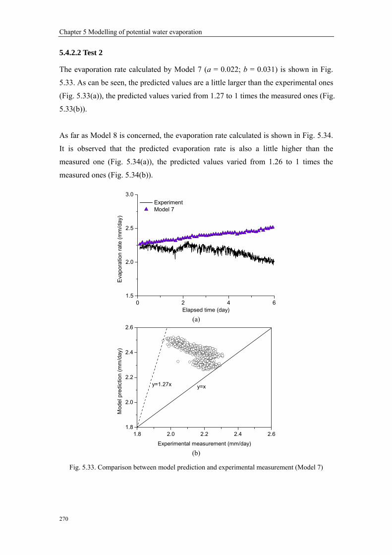
Chapter 5 Modelling of potential water evaporation
270
5.4.2.2 Test 2
The evaporation rate calculated by Model 7 (a = 0.022; b = 0.031) is shown in Fig.
5.33. As can be seen, the predicted values are a little larger than the experimental ones
(Fig. 5.33(a)), the predicted values varied from 1.27 to 1 times the measured ones (Fig.
5.33(b)).
As far as Model 8 is concerned, the evaporation rate calculated is shown in Fig. 5.34.
It is observed that the predicted evaporation rate is also a little higher than the
measured one (Fig. 5.34(a)), the predicted values varied from 1.26 to 1 times the
measured ones (Fig. 5.34(b)).
0 2 4 61.5
2.0
2.5
3.0
Evap
orat
ion
rate
(mm
/day
)
Elapsed time (day)
Experiment Model 7
(a)
1.8 2.0 2.2 2.4 2.61.8
2.0
2.2
2.4
2.6
Mod
el p
redi
ctio
n (m
m/d
ay)
Experimental measurement (mm/day)
y=xy=1.27x
(b)
Fig. 5.33. Comparison between model prediction and experimental measurement (Model 7)

Chapter 5 Modelling of potential water evaporation
271
0 2 4 61.5
2.0
2.5
3.0
Evap
orat
ion
rate
(mm
/day
)
Elapsed time (day)
Experiment Model 8
(a)
1.8 2.0 2.2 2.4 2.61.8
2.0
2.2
2.4
2.6
Mod
el p
redi
ctio
n (m
m/d
ay)
Experimental measurement (mm/day)
y=xy=1.26x
(b)
Fig. 5.34. Comparison between model prediction and experimental measurement (Model 8)
5.4.2.3 Test 3
The comparison between the evaporation rate calculated by Model 7 (a = 0.022, b =
0.031) and the measured one is shown in Fig. 5.35. As can be seen, the predicted
values are inconsistent with the experimental ones (Fig. 5.35(a)), the predicted values
varied from 1.27 to 0.87 times the measured ones (Fig. 5.35(b)).
As for Model 8, the evaporation rate calculated is shown in Fig. 5.36. It is observed
that the predicted evaporation rate is a little higher or lower than the measured one
(Fig. 5.36(a)), the predicted values varied from 1.29 to 0.89 times the measured ones.
(Fig. 5.36(b)).

Chapter 5 Modelling of potential water evaporation
272
0 1 2 3 4 5 6 71.0
1.5
2.0
2.5
Evap
orat
ion
rate
(mm
/day
)
Elapsed time (day)
Experiment Model 7
(a)
1.2 1.4 1.6 1.8 2.01.2
1.4
1.6
1.8
2.0
Mod
el p
redi
ctio
n (m
m/d
ay)
Experimental measurement (mm/day)
y=x
y=0.87x
y=1.27x
(b)
Fig. 5.35. Comparison between model prediction and experimental measurement (Model 7)
0 1 2 3 4 5 6 71.0
1.5
2.0
2.5
Evap
orat
ion
rate
(mm
/day
)
Elapsed time (day)
Experiment Model 8
(a)

Chapter 5 Modelling of potential water evaporation
273
1.2 1.4 1.6 1.8 2.01.2
1.4
1.6
1.8
2.0
Mod
el p
redi
ctio
n (m
m/d
ay)
Experimental measurement (mm/day)
y=x
y=1.29x
y=0.89x
(b)
Fig. 5.36. Comparison between model prediction and experimental measurement (Model 8)
5.4.2.4 Test 4
Model 7 is used to predict the potential evaporation in Test 4. As can be seen in Fig.
5.37, the evaporation rate calculated by Model 7 (a = 0.022; b = 0.031) is higher or
lower than the experimental one (Fig. 5.37(a)), the predicted values varied from 1.07
to 0.92 times the measured ones (Fig. 5.37(b)).
As for Model 8, the evaporation rate calculated is also inconsistent with the measured
one (Fig. 5.38(a)), the predicted values varied from 1.1 to 0.91 times the measured
ones (Fig. 5.38(b)).
0 2 4 61.2
1.4
1.6
1.8
2.0
2.2
2.4
2.6
Eva
pora
tion
rate
(mm
/day
)
Elapsed time (day)
Experiment Model 7
(a)

Chapter 5 Modelling of potential water evaporation
274
1.6 1.8 2.0 2.2 2.41.6
1.8
2.0
2.2
2.4
Mod
el p
redi
ctio
n (m
m/d
ay)
Experimental measurement (mm/day)
y=xy=1.07x
y=0.92x
(b)
Fig. 5.37. Comparison between model prediction and experimental measurement (Model 7)
0 2 4 61.2
1.4
1.6
1.8
2.0
2.2
2.4
2.6
Evap
orat
ion
rate
(mm
/day
)
Elapsed time (day)
Experiment Model 8
(a)
1.6 1.8 2.0 2.2 2.41.6
1.8
2.0
2.2
2.4
Mod
el p
redi
ctio
n (m
m/d
ay)
Experimental measurement (mm/day)
y=xy=1.1x
y=0.91x
(b)
Fig. 5.38. Comparison between model prediction and experimental measurement (Model 8)

Chapter 5 Modelling of potential water evaporation
275
5.5 Conclusion
This chapter is devoted to the assessment of the existing models for potential
evaporation. Various models reported in the literature have been assessed based on the
experimental data from the free water evaporation test with different atmospheric
conditions, along with some extended models that correspond to different
combinations of some existing models. The related parameters of these models were
firstly determined using part of the experimental data, and then the models with the
determined parameters were verified with another part of data. On the whole, part of
these models can give a perfect prediction of evaporation rate under the condition of
different wind speeds and part of them can show good performance in predicting the
potential evaporation rate at different temperatures. It appears that Models 7 and 8 are
the most relevant, allowing satisfactory prediction under different atmospheric
conditions. In reality, in the range of wind speed considered in the test performed in
this study (0 - 0.5 m/s), the effect of wind speed is quite similar in Model 7 and Model
8. As mentioned in Chapter 1, the evaporation rate increases linearly with the
increasing wind speed in a large range of wind speed (Wang, 2006). Therefore, Model
7 is selected as the potential evaporation model in this study for further development.
More specific conclusions drawn are as follows:
1. The models considering wind speed and vapor pressure (Models 1, 2, and 3) give a
good prediction when the experiment was conducted at different wind speeds.
However, bad results can be obtained when using them in case of different
temperatures.
2. The model only considering air temperature and relative humidity at a reference
height (Model 6) is suitable for predicting the potential evaporation rate in case of
different temperatures. However, it cannot be used for different wind speeds.
3. The models considering wind speed, vapor pressure and air temperature (Models 4
and 5) are not suitable for predicting evaporation rate.
4. The model proposed by Ta (2009) appears to be the best one.

Chapter 5 Modelling of potential water evaporation
276
5. The models considering wind speed usually give a good prediction in case of
varying wind speed.
6. The functions of wind speed and temperature have strong influence on the potential
evaporation rate than that of vapor pressure.
7. The form of wind speed function in different models (e.g., linear or natural
logarithm) has less influence when the wind speed range is limited.

Chapter 6 Modelling of actual water evaporation from sand and clay
277
Chapter 6 Modelling of actual water evaporation from sand
and clay
6.1 Introduction
Various models for predicting water evaporation from soils were discussed in Chapter
1. Each model has its advantages and disadvantages. On the whole, for selecting a
suitable water evaporation model, its application field needs to be examined carefully.
Considering the experiential conditions in this study, the water balance model is not
found suitable. As can be seen through the profiles of both air and soil temperatures
from the evaporation tests on Fontainebleau sand and Héricourt clay, the laboratory
temperature has significant influence on the temperature inside the chamber,
indicating that heat exchange existed between the environmental chamber and the
laboratory ambiance. Thus, the energy balance related models are not suitable for
predicting water evaporation using the data obtained with this chamber. As no dry soil
column was taken as a reference sample in the tests, the application of the
Three-temperature model is also limited. Furthermore, the effect of crack cannot be
considered in Three-temperature model. By contrast, the mass transfer model was
found to be relevant for predicting potential evaporation. Thus, a modified mass
transfer model was selected in Chapter 5 for describing the potential evaporation
based on the data obtained with the environmental chamber. The resistance model
gives a clear physical meaning of water vapor traveling from soil to atmosphere. But
the prediction results are too sensitive to the selected value of resistance. Moreover,
the soil resistance depends on the soil conditions (soil type, depth of soil considered)
and hence restricting its utilization – it is difficult to define the boundary condition in
a numerical analysis using this kind of models. By contrast, the suction related model
proposed by Aydin et al. (2005) is simple, but the related parameters are not easy to
be determined and the effect of cracks cannot be taken into account. For the suction
related models proposed by Campbell (1985), Wilson et al. (1997) and Ta (2009),
their forms are simple and they contain both soil and atmospheric parameters. The
parameter of surface suction makes these models independent of soil properties such
as soil texture and mineralogy. Furthermore, Ta (2009) attempted to extend his model

Chapter 6 Modelling of actual water evaporation from sand and clay
278
to the effects of cracks. His model has been selected in this study as the basis for the
development of water evaporation model.
In this chapter, the model proposed by Campbell (1985), Wilson et al. (1997) and Ta
(2009) will be assessed based on the experimental data obtained and presented in
Chapter 4. A new model is then proposed for predicting water evaporation from sand.
The related parameters will be determined using the data from the four evaporation
tests conducted under different atmospheric conditions. Furthermore, the performance
of this new model is also verified based on the data from the sand evaporation tests.
On the other hand, a new model accounting for the effect of cracks is also proposed.
After determining the parameters, the relevance of the new model is also verified
based on the data from the clay evaporation tests.
6.2 Model for water evaporation from sand
6.2.1 Verification of the selected suction related models
As discussed in Chapter 1, the suction related models have a simple form and can
consider both the influences of soil and atmospheric parameters. More specifically,
they are independent of soil texture and mineralogy. In this section, the models
proposed by Campbell (1985), Wilson et al. (1997) and Ta (2009) are first verified
using the experimental data before developing a new model. A general form of these
models is shown in Equation 6.1.
a s a
p a1E h hE h
−=
− (6.1)
where Ea is the actual evaporation rate (mm/day); Ep is the potential evaporation rate
which can be determined by Model 7 in Chapter 5 (mm/day); hs is the relative
humidity at the soil evaporating surface (%); ha is the air relative humidity at a
reference level (%). Note that hs can be determined by Kelvin’s equation when the
soil suction is known.
The data obtained from the four Fontainebleau sand evaporation tests were used to
assess the performance of Equation 6.1. The details of these data were shown in
Chapter 3. For determining the relative humidity at the soil evaporating surface, hs,

Chapter 6 Modelling of actual water evaporation from sand and clay
279
the directly measured near surface suction was used after converting to the relative
humidity using Kelvin’s equation with the soil temperature at this position. Notably,
due to the limited measurement range of the tensiometers used, all the suctions
measured are lower than 1.5 MPa. For the relative humidity at the reference level, the
measurement of T3111 transmitter at 50-mm height is considered. As mentioned
before, the potential evaporation rate (Ep) is calculated by Model 7 (see Chapter 5)
using the measured wind speed and relative humidity at the reference level (50 mm
above soil surface). Finally, the actual evaporation rate is calculated using Equation
6.1. The evolutions of the predicted and measured actual evaporation rates in different
evaporation tests are shown in Fig. 6.1.
0 6 12 18 24 300.0
0.5
1.0
1.5
2.0
2.5
3.0
Eva
pora
tion
rate
(mm
/day
)
Elapsed time (day)
Experiment Equation 6.1
(a) Test 1
0 6 12 18 24 300.0
0.5
1.0
1.5
2.0
2.5
3.0E
vapo
ratio
n ra
te (m
m/d
ay)
Elapsed time (day)
Experiment Equation 6.1
(b) Test 2
0 6 12 18 24 300.0
0.5
1.0
1.5
2.0
2.5
3.0
Eva
pora
tion
rate
(mm
/day
)
Elapsed time (day)
Experiment Equation 6.1
(c) Test 3
0 6 12 18 24 300.0
0.5
1.0
1.5
2.0
2.5
3.0
Eap
orat
ion
rate
(mm
/day
)
Elapsed time (day)
Experiment Equation 6.1
(d) Test 4
Fig. 6.1. Evolutions of the predicted and measured actual evaporation rates in different evaporation tests on the Fontainebleau sand
As can be seen in Fig. 6.1, the predicted evaporation rate is higher than the measured
one. In particular, the predicted values are much larger than the measured ones in the
falling-rate stage evaporation. Only in Test 4 the predicted evaporation rate is

Chapter 6 Modelling of actual water evaporation from sand and clay
280
consistence with the measured one in the first six days. Therefore, it can be deduced
that predicting evaporation rate using the directly measured near surface suction is not
suitable, even though the suction measured is close to the soil surface. In other words,
the suction at soil surface (evaporating surface) should be much larger than at the
measurement level. Furthermore, the formation of a dry soil layer and its progress
during evaporation is not considered in this model. As discussed in Chapter 1, the
effect of the dry soil layer on water evaporation can be quite strong in case of sand.
6.2.2 Modification of the existing suction related model
6.2.2.1 Using air relative humidity close to the soil surface
As deduced in the last section, the prediction of evaporation rate using suction related
model (Equation 6.1) with the suction measured in the zone close to the soil surface is
larger than the measured one. This is because the suction close to the soil surface
cannot represent the real suction at the soil surface (evaporating surface). On the other
hand, the air relative humidity at 5 mm above soil surface was measured. Therefore,
in this section, the relative humidity measured at 5 mm above the soil surface is used
to predict the evaporation rate using Equation 6.1. Figure 6.2 shows the comparison of
the measured and predicted evaporation rates.
0 6 12 18 24 300.0
0.5
1.0
1.5
2.0
2.5
Evap
orat
ion
rate
(mm
/day
)
Elapsed time (day)
Experiment Equation 6.1
(a) Test 1
0 6 12 18 24 300.0
0.5
1.0
1.5
2.0
2.5
Eapo
ratio
n ra
te (m
m/d
ay)
Elapsed time (day)
Experiment Equation 6.1
(b) Test 2

Chapter 6 Modelling of actual water evaporation from sand and clay
281
0 6 12 18 24 300.0
0.5
1.0
1.5
2.0
2.5
Evap
orat
ion
rate
(mm
/day
)
Elapsed time (day)
Experiment Equation 6.1
(c) Test 3
0 6 12 18 24 300.0
0.5
1.0
1.5
2.0
2.5
Evap
orat
ion
rate
(mm
/day
)
Elapsed time (day)
Experiment Equation 6.1
(d) Test4
Fig. 6.2. Comparison between the measured evaporation rate and the predicted one using the relative humidity at 5-mm height
As can be seen in Fig. 6.2, the predicted evaporation rate is lower than the measured
one and the difference between them becomes smaller along with the evaporation
process. It can be then deduced that the real relative humidity at soil surface is much
larger than the one at 5-mm height. Indeed, the soil surface (evaporating surface)
relative humidity calculated using Equation 6.1 with the measured actual evaporation
rate is much higher than the one at 5-mm height (see Fig. 6.3), especially at the
constant-rate stage evaporation. Thus, directly using the air relative humidity at a
position close to the soil surface is not suitable for predicting the actual evaporation
rate using Equation 6.1. Furthermore, taking an air relative humidity as the boundary
condition is not appropriate physically.
0 6 12 18 24 300
20
40
60
80
100
120
Rel
ativ
e hu
mid
ity (%
)
Elapsed time (day)
Soil surface 5-mm height 50-mm height
(a) Test 1
0 6 12 18 24 300
20
40
60
80
100
120
Rel
ativ
e hu
mid
ity (%
)
Elapsed time (day)
Soil surface 5-mm height 50-mm height
(b) Test 2

Chapter 6 Modelling of actual water evaporation from sand and clay
282
0 6 12 18 24 300
20
40
60
80
100
120
Rel
ativ
e hu
mid
ity (%
)
Elapsed time (day)
Soil surface 5-mm height 50-mm height
(c) Test 3
0 6 12 18 24 300
20
40
60
80
100
120
Rel
ativ
e hu
mid
ity (%
)
Elapsed time (day)
Soil surface 5-mm height 50-mm height
(d) Test 4
Fig. 6.3. Evolutions of relative humidity at different positions
6.2.2.2 Development of a new model and its parameters determination
1. Development of a new model
Fig. 6.4. The process of evaporation from soil with dry layer
(Re-edited from Yamanaka et al., 1997) As presented in Chapter 1, upon soil water evaporation, once a dry soil layer is
formed, the evaporation process mainly occurs at the bottom of the dry soil layer (i.e.,
drying or evaporating surface). Therefore, a three-stage water vapor transport process
can be identified (Fig. 6.4): (1) water vapor is carried out from the water surface to the
drying surface (evaporating surface); (2) water vapor is transported from the drying
surface to the soil surface by vapor diffusion and (3) water vapor travels from the soil
surface to atmosphere under the restriction of aerodynamic resistance. On this basis,

Chapter 6 Modelling of actual water evaporation from sand and clay
283
the relative humidity at soil surface can be defined as h_surface, the relative humidity at
the drying surface (evaporating surface) is considered as h_drying, and the air relative
humidity at the reference level is ha. For the suction related model proposed by
Campbell (1985), Wilson et al. (1997) and Ta (2009) (Equation 6.1), the variable hs
represents the relative humidity at the drying (or evaporating) surface. Thus, we
assume that the drying surface keeps at the soil surface during the evaporation process.
This leads to:
a surface a
p a
_100
E h hE h
−=
− (6.2)
The relative humidity at the soil surface (h_surface) consists of two parts: the first part
induced by the water vapor transported from the drying surface at a certain depth
(h_wet) and the water vapor from the dry soil layer (h_dry):
surface wet dry_ _ _h h h= + (6.3)
In general, the water content in the dry soil layer is relatively low, and its contribution
to the surface relative humidity can be neglected. Assuming h_dry = 0, we obtain:
surface wet_ _h h= (6.4)
As far as the transportation of water vapor in the dry soil layer is concerned, it is
mainly affected by the soil resistance which is related to soil structure or porosity.
Assuming that the soil resistance is the same within the dry soil layer, and then the air
relative humidity decreases along with the transportation path from the drying surface
to the soil surface. Therefore, we can reasonably assume that the relative humidity
inside the dry soil layer is a function of the depth of dry soil layer (d):
drying wet drying surface_ _ _ _ ( )h h h h f d− = − = (6.5)
Or
surface drying_ _ ( )h h f d= − (6.6)
Finally, we obtain the expression of the new model taking the dry layer into account:
drying aa
p a
( _ ( ))100
h f d hEE h
− −=
− (6.7)
2. Parameter determination
As can be seen from the water retention curve in Chapter 3, the matric suction
increases with the decrease of water content. However, once the suction exceeds

Chapter 6 Modelling of actual water evaporation from sand and clay
284
40 kPa, its value increases quickly with further decrease of water content. Under this
condition, water inside the soil becomes discontinuous and will be transported in the
form of vapor in soil. On the other hand, the value of matric suction of 40 kPa
corresponds to a volumetric water of 5 %. Therefore, once the volumetric water
content is lower than 5 %, we can suppose that the soil becomes dry and the depth
corresponding to this water content can be considered as the position of the drying
surface. Note however that in reality, there is still some water existing inside the dry
soil layer, but as discussed above its contribution to evaporation can be neglected.
Based on this consideration, the evolution of the drying surface during evaporation
can be obtained (see Fig. 6.5). Thereby, the relationship between the elapsed time and
the depth of dry soil layer can be easily obtained. This relationship is shown in Fig.
6.5.
0 6 12 18 24 300.0
0.5
1.0
1.5
2.0
2.5
Actual evaporation rate Depth of dry soil layer
Elapsed time (day)
Actu
al e
vapo
ratio
n ra
te (m
m/d
ay)
0
1
2
3
4
5
6
7
Dep
th o
f dry
soi
l lay
er (m
m)
(a) Test 1
0 6 12 18 24 300.0
0.5
1.0
1.5
2.0
2.5
Actual evaporation rate Depth of dry soil layer
Elapsed time (day)
Actu
al e
vapo
ratio
n ra
te (m
m/d
ay)
0
2
4
6
8
10
12
14
16
Dep
th o
f dry
soi
l lay
er (m
m)
(b) Test 2
0 6 12 18 24 300.0
0.5
1.0
1.5
2.0
2.5
Actual evaporation rate Depth of dry soil layer
Elapsed time (day)
Actu
al e
vapo
ratio
n ra
te (m
m/d
ay)
0
2
4
6
8
10
12
14
16
18
Dep
th o
f dry
soi
l lay
er (m
m)
(c) Test 3
0 6 12 18 24 300.0
0.5
1.0
1.5
2.0
2.5
Actual evaporation rate Depth of dry soil layer
Elapsed time (day)
Act
ual e
vapo
ratio
n ra
te (m
m/d
ay)
0
5
10
15
20
25 D
epth
of d
ry s
oil l
ayer
(mm
)
(d) Test 4
Fig. 6.5. Evolutions of actual evaporation rate and depth of dry soil layer
As can be seen in Fig. 6.5, the depth of dry soil layer increases with the decrease of
actual evaporation rate from the falling-rate stage to the end of the test. This result
confirms that the dry soil layer has significant influence on the evaporation process.

Chapter 6 Modelling of actual water evaporation from sand and clay
285
0 2 4 6 8 10 120.0
0.2
0.4
0.6
0.8
1.0
1.2E
a/Ep
Elapsed time (day)
(a) Test 1
0 2 4 6 8 10 120.0
0.2
0.4
0.6
0.8
1.0
1.2
E a/Ep
Elapsed time (day)
(b) Test 2
0 2 4 6 8 10 12 14 16 180.0
0.2
0.4
0.6
0.8
1.0
1.2
Ea/E
p
Elapsed time (day) (c) Test 3
0 5 10 15 20 25 300.0
0.2
0.4
0.6
0.8
1.0
1.2
E a/Ep
Elapsed time (day) (d) Test 4
Fig. 6.6. Evolutions of Ea/Ep
With the potential evaporation Ep calculated by Model 7, the ratio Ea/Ep can be
determined. Figure 6.6 shows the evolutions of this ratio for the four tests on sand. It
is observed that the value of Ea/Ep is not equal to 1 during the constant-rate stage and
this result is in conflict with the theory. Therefore, the potential evaporation rate
predicted using Model 7 needs to be adjusted. For this purpose, we multiple Ep by a
constant parameter and then the average value of Ea/Ep before the occurrence of dry
soil layer should be equal to 1. The constant parameters in the four tests are 0.83, 0.92,
0.9, and 1.0, respectively. Furthermore, these values are consistent with the
relationship between the predicted and measured evaporation rates shown in Chapter
5.
For investigating the relationship between the relative humidity inside the dry soil
layer and the depth of dry soil layer, the soil surface relative humidity (h_surface) is first
calculated by Equations 6.1 using the measured experimental data. The relative

Chapter 6 Modelling of actual water evaporation from sand and clay
286
humidity at the drying surface (h_drying) can be deduced using the water retention curve
based on the volumetric water content at this position. In this study, the volumetric
water content at drying surface is close to 5 %, corresponding to a suction of 40 kPa.
Using Kelvin’s equation, this suction can be converted to relative humidity by
considering the temperature at the position of drying surface. The depth of dry soil
layer can be calculated by the relationship between the depth of dry soil layer and the
elapsed time (Fig. 6.5). Finally, the relationship between h_drying-h_surface and d can be
obtained for different tests (Fig. 6.7). As can be seen, a series of fitting curves are
obtained. This result confirms that there is indeed a relationship between the soil
relative humidity and the depth of dry soil layer. A summary of the functions of these
fitting curves are listed in Table 6.1.
Table 6.1 Various expressions of f(d) in different tests
Number f(d) Remark
Test 1 f(d) = 43.73+(6.56-43.73)/(1+exp((d-7.14)/1.24))
Test 2 f(d) = 75.75+(9.07-75.75)/(1+exp((d-12.86)/1.41))
Test 3 f(d) = 60.89+(7.36-60.89)/(1+exp((d-14.38)/1.41))
Test 4 f(d) = 82.09+(6.38-82.09)/(1+exp((d-16.11)/1.69))
Tests 1 to 4 f(d) = 90.98+(6.33-90.98)/(1+exp((d-15.94)/2.85))
h_drying-h_surface = f(d)
0 2 4 6 80
5
10
15
20
25
30
h _dry
ing-h
_sur
face
(%)
d (mm)
(a) Test 1
0 2 4 6 8 10 12 14 16 180
10
20
30
40
50
60
70
h _dry
ing-h _s
urfa
ce (%
)
d (mm)
(b) Test 2

Chapter 6 Modelling of actual water evaporation from sand and clay
287
0 2 4 6 8 10 12 14 16 180
10
20
30
40
50
60
70
h _dry
ing-h
_sur
face
(%)
d (mm)
(c) Test 3
0 4 8 12 16 20 240
20
40
60
80
100
h _dry
ing-h
_sur
face
(%)
d (mm)
(d) Test 4
0 6 12 18 240
20
40
60
80
100
h _dry
ing-h
_sur
face
(%)
d (mm)
(e) All the four tests
Fig. 6.7. Relationships between h_drying-h_surface and d in different tests
6.2.3 Verification of the new actual evaporation model
For verifying the new model proposed, after obtaining the expression of function f(d),
Equation 6.7 is used to determine the actual evaporation. In the evaporation process,
before the occurrence of dry soil layer, the relative humidity at the soil surface is
equal to the one at the drying surface (h_surface = h_drying). Therefore, the surface
volumetric water content can be extrapolated from the volumetric water content
profile, and the surface suction can be calculated in turn using the water retention
curve. Afterwards, the relative humidity at the soil surface can be obtained using
Kelvin’s equation. Once the dry soil layer appears, the relative humidity at the drying
surface is considered as the relative humidity corresponding to 40 kPa suction at the
drying surface temperature. After determining all the parameters of Equation 6.7, the
verification procedure can start. Firstly, the actual evaporation rate in a test is
predicted using the corresponding expression of f(d). The comparison between the
measured and predicted actual evaporation rates are shown in Fig. 6.8. Secondly, for

Chapter 6 Modelling of actual water evaporation from sand and clay
288
verifying the new model, the average function f(d) obtained from all the four tests
(Fig. 6.7(e)) is selected and Equation 6.7 is used to predict the actual evaporation rate.
Note that the predicted evaporation before the dry soil layer occurrence is the same as
that in Fig. 6.8. As can be seen in Fig. 6.8, the predicted actual evaporation rate is
consistent with the measured one, especially after the occurrence of dry soil layer.
However, the actual evaporation rate predicted increases over time before the
formation of the dry layer. As shown in Fig. 6.9, the predicted results in tests 3 and 4
show consistent evolution trends with the measured ones. On the contrary, large
deviation can be observed in Tests 1 and 2.
0 6 12 18 24 300.0
0.5
1.0
1.5
2.0
2.5
3.0
Eva
pora
tion
rate
(mm
/day
)
Elapsed time (day)
Experiment Equation 6.7
(a) Test 1
0 6 12 18 24 300.0
0.5
1.0
1.5
2.0
2.5
3.0
Evap
orat
ion
rate
(mm
/day
)
Elapsed time (day)
Experiment Equation 6.7
(b) Test 2
0 6 12 18 24 300.0
0.5
1.0
1.5
2.0
2.5
3.0
Eva
pora
tion
rate
(mm
/day
)
Elapsed time (day)
Experiment Equation 6.7
(c) Test 3
0 5 10 15 20 25 300.0
0.5
1.0
1.5
2.0
2.5
3.0
Eapo
ratio
n ra
te (m
m/d
ay)
Elapsed time (day)
Experiment Equation 6.7
(d) Test 4
Fig. 6.8. Comparison between the measured and predicted actual evaporation rates using different functions f(d)

Chapter 6 Modelling of actual water evaporation from sand and clay
289
0 6 12 18 24 300.0
0.5
1.0
1.5
2.0
2.5
3.0
Evap
orat
ion
rate
(mm
/day
)
Elapsed time (day)
Experiment Equation 6.7
(a) Test 1
0 6 12 18 24 300.0
0.5
1.0
1.5
2.0
2.5
3.0
Eva
pora
tion
rate
(mm
/day
)
Elapsed time (day)
Experiment Equation 6.7
(b) Test 2
0 6 12 18 24 300.0
0.5
1.0
1.5
2.0
2.5
3.0
Eva
pora
tion
rate
(mm
/day
)
Elapsed time (day)
Experiment Equation 6.7
(c) Test 3
0 6 12 18 24 300.0
0.5
1.0
1.5
2.0
2.5
3.0
Eap
orat
ion
rate
(mm
/day
)
Elapsed time (day)
Experiment Equation 6.7
(c) Test 4
Fig. 6.9. Comparison between the measured and predicted actual evaporation rates by a unique average function f(d)
6.2.4 Discussion
In this section, the function of dry soil layer depth f(d) is introduced in the suction
related models, defining a new actual evaporation prediction model. The verification
of this new model has been undertaken. As can be seen in Fig. 6.8, the predicted
values are consistent with the measured ones when using a specific function of f(d) for
each test, and the effect of dry soil layer on soil water evaporation can be considered
effectively. This confirms the relevance of this model. However, when a unique
average function is used, only part of the tests can be simulated satisfactorily. This is
due to the variation of the relationship between the relative humidity and the depth of
dry soil layer (i.e., f(d)) in different tests. Basically, this relationship should be unique.
However, during different tests, the infiltration-evaporation cycle may induce some
modification of the soil sample, hence creating some heterogeneity in it and defining
variable f(d) functions. As far as the predicted results before the occurrence of dry soil
layer is concerned, distinct deviation can be observed in Figs. 6.8 and 6.9.

Chapter 6 Modelling of actual water evaporation from sand and clay
290
Furthermore, the predicted actual evaporation rate increases gradually in this stage.
This phenomenon may be explained as follows: the accuracy of suction measurement
needs to be improved in the near surface zone because in this stage, the relative
humidity is high, close to 100%, and a little change in relative humidity can cause
significant change in suction. On the other hand, the suction in this zone is difficult to
determine using simple equation like Equation 6.1. Indeed, the suction deduced by
Equation 6.1 using the measured actual evaporation rate shows that the predicted
surface suction is higher than 1 MPa in different tests (Fig. 6.10). As we know, for
sand as pure as the Fontainebleau sand, any suction exceeding 100 kPa does not make
sense.
0 6 12 18 24 300.01
0.1
1
10
100
1000
Suct
ion
(MPa
)
Elapsed time (day)
(a) Test 1
0 6 12 18 24 300.1
1
10
100
1000S
uctio
n (M
Pa)
Elapsed time (day)
(b) Test 2
0 6 12 18 24 300.01
0.1
1
10
100
1000
Suc
tion
(MP
a)
Elapsed time (day)
(c) Test 3
0 6 12 18 24 300.1
1
10
100
1000
Suc
tion
(MP
a)
Elapsed time (day)
(d) Test 4
Fig. 6.10. Surface suction deduced from actual evaporation using Equation 6.1

Chapter 6 Modelling of actual water evaporation from sand and clay
291
6.3 Model for water evaporation from clay
6.3.1 Proposed model
6.3.1.1 Verification of the existing model
0 5 10 15 20 250
1
2
3
Eva
pora
tion
rate
(mm
/day
)
Elapsed time (day)
Experiment Equation 6.1
Fig. 6.11. Comparison between the measured and predicted actual evaporation rates
0 10 20 30 40 50 60 70 80 900
20
40
60
80
100
120
Rel
ativ
e hu
mid
ity (%
)
Elapsed time (day)
Soil surface (predicted) 50-mm depth
Fig. 6.12. Relative humidity evolutions at different positions
As a general form of suction related model, Equation 6.1 is verified using the data
obtained from the first Héricourt clay evaporation test. The suction directly measured
in the zone near the soil surface is firstly used to predict the actual evaporation using
Equation 6.1. Figure 6.11 shows the comparison between the measured and predicted
actual evaporation rates. As can be seen, the predicted value increases gradually and is
much higher than the measured one after the constant-rate evaporation stage. This
means that the relative humidity at the soil surface is much higher than the one
deduced from the suction at the position close to the soil surface. Thus, the surface
suction needs to be determined more accurately. On the other hand, the soil surface
relative humidity can also be deduced from Equation 6.1 using the measured actual
evaporation rate. As can be seen in Fig. 6.12, the predicted relative humidity is much
higher than the one at 50-mm height, even at the end of test. As shown in Chapter 4,
the actual evaporation rate at the slow-rate evaporation stage is extremely low, equal
to 0.3 mm/day. Basically, once the evaporation rate is close to stabilization, the
relative humidity at the soil surface will approach the one in the air. The phenomenon
observed in Fig. 6.12 may be attributed to the occurrence of cracks during evaporation,
because the cracks allow water to evaporate from them, hence increasing the relative
humidity at the soil surface. Similar result was also reported by Ta (2009). In

Chapter 6 Modelling of actual water evaporation from sand and clay
292
conclusion, accurately determining the soil surface suction is essential for the actual
evaporation prediction. Moreover, the suction related model should be extended to the
effect of cracks.
6.3.1.2 Development of a new model
Fig .6.13. Water evaporation from cracked soil
Figure 6.13 presents the water evaporation mechanism from cracked soil. Once cracks
occur, water can evaporate in two ways: (1) directly from the soil surface without
cracks; (2) from the walls of cracks. As in the case of water evaporation from sand,
we define the relative humidity at the soil surface as h_surface. It consists of two parts:
the relative humidity of non-cracked soil (h_non-crack) and the relative humidity of
cracks (h_crack). Note that h_crack is an equivalent value of the relative humidity inside
cracks. When the soil is dry, the value of h_crack is much higher than that of h_non-crack.
For simplicity, we assume:
_crack _non-crackh kh= (6.8)
By considering the soil surface crack ratio (R), we can obtained:
_surface _ crack _ crack= +(1- ) nonh Rh R h − (6.9)
Or _surface _ crack= (1+( -1) ) nonh k R h − (6.10)
Combining Equations 6.2 and 6.10 leads to:
Reference level ha
h_non-crack h_crack
Soil
h_surface
Crack Water vapor in cracks

Chapter 6 Modelling of actual water evaporation from sand and clay
293
_ aa
p a
(1+( -1) )100-
non crackk R h hEE h
− −= (6.11)
Particularly, when the soil is dry, water vapor from cracks has more contribution to
the relative humidity at the soil surface than from the non-cracked soil. Thereby, in
this case, we can assume that h_non-crack is equal to ha, giving:
_surface a= (1+ )h kR R h− (6.12)
Note that the unit of relative humidity in these equations is percentage (%), and the
surface crack ratio (R) is in decimal form.
6.3.2 Parameters determination and model verification
0 10 20 30 40 50 60 70 80 900.0
0.5
1.0
1.5
E a/Ep
Elapsed time (day)
(a) The first evaporation test
12 18 24 30 36 42 48 540.0
0.5
1.0
1.5E
a/Ep
Elapsed time (day)
(b) The second evaporation test
Fig. 6.14. Ea/Ep during the two tests
After determining the potential evaporation Ep using Model 7, the ratio Ea/Ep can be
then determined for the two Héricourt clay evaporation tests. Figure 6.14 shows the
evolutions of this ratio during the two tests. Notably, the second Héricourt clay
evaporation test started after a free water evaporation; therefore, the initiation of soil
evaporation test was after t = 12.8 days. As can be seen in Fig. 6.14, the value of Ea/Ep
is also not equal to 1 during the constant-rate stage. Therefore, as in the case of sand,
we multiply Ep by a constant parameter so that the average value of Ea/Ep during the
constant-rate evaporation stage is equal to 1. The values of 1.15 and 1.2 are obtained
for the first and the second tests, respectively. Note that these values are consistent
with the relationship between the predicted and measured evaporation rate shown in
Chapter 5.

Chapter 6 Modelling of actual water evaporation from sand and clay
294
For determining parameter k, the surface relative humidity predicted using Equation
6.2 with the adjusted potential evaporation rate is firstly compared with the one
measured at 50-mm height (Fig. 6.15). Afterwards, parameter k can be calculated by
Equation 6.12 with the known surface crack ratio (R) (Fig. 6.16). It is worth noting
that the surface crack ratio is the total crack area divided by the whole soil surface
area. It is a little different from the one in Chapter 4. The calculation of the surface
crack ratio in Chapter 4 does not take the cracks at boundary into account. For the
first evaporation test, the data shown in Fig. 6.15(a) from t = 65 days to t = 84 days
are selected for the calculation of k. Note that the surface crack ratio during this stage
is 25.5 %. Finally, the parameter in this test can be determined: k = 3.65. For the
second evaporation test, the data shown in Fig. 6.15(b) from t = 43 days to t = 54 days
are selected for the calculation of k. The corresponding surface crack ratio is 29 %. A
value of k = 5.59 is obtained.
0 10 20 30 40 50 60 70 80 900
20
40
60
80
100
120
Rel
ativ
e hu
mid
ity (%
)
Elapsed time (day)
h_surface (with cracks) 50-mm height
(a) The first evaporation test
12 18 24 30 36 42 48 540
20
40
60
80
100
120
Rel
ativ
e hu
mid
ity (%
)
Elapsed time (day)
50-mm height h_surface (with cracks)
(b) The second evaporation test
Fig. 6.15. Evolutions of the predicted and measured relative humidity in different tests
0 10 20 30 40 50 60 70 80 900
5
10
15
20
25
30
Surfa
ce c
rack
ratio
(%)
Elapsed time (day)
(a) The first evaporation test
12 18 24 30 36 42 48 540
5
10
15
20
25
30
35
Surfa
ce c
rack
ratio
(%)
Elapsed time (day)
(b) The second evaporation test
Fig. 6.16. Evolutions of surface crack ratio in different tests

Chapter 6 Modelling of actual water evaporation from sand and clay
295
After determining the related parameter of the new model (Equation 6.11), the
application of this model is then undertaken. The first Héricourt clay evaporation test
is taken as an example. Two methods are used for this purpose (Method 1 and Method
2). In Method 1, the volumetric water content at the soil surface (Fig. 6.17) is firstly
extrapolated from the water content profile shown in Chapter 4. Then, the soil surface
suction is calculated by the water retention curve. Due to the incomplete data, a
virtual water retention curve which covers the suction range being obtained in this test
is adopted (Fig. 6.18). This water retention curve is fitted by the model proposed by
Fredlund and Xing (1994) (see Equation 3.1). More specifically, the saturated
volumetric water content (θs) is 65 %, and the residual volumetric water content (θr) is
1 %. For the three fitting parameters a, n and m, they are 50, 0.65 and 7, respectively.
As shown in Fig. 6.17, the extrapolated water content can reach nearly 1 %,
suggesting that taking 1 % as the residual volumetric water content is reasonable.
After that, the soil surface suction is converted to the surface relative humidity using
Kelvin’s equation. Note that this surface relative humidity corresponds to value at the
soil surface without cracks, i.e., h_non-crack in Equation 6.11. Finally, with the
determined k, h_non-crack, potential evaporation rate and the measured air relative
humidity at the reference level (ha), the actual evaporation rate can be determined by
Equation 6.11 (Fig. 6.19). Notably, as the water content after t = 40 days is quite low
(close to 1 %), the relative humidity at the soil surface (h_non-crack) is taken equal to the
one at the reference level when using Equation 6.11 to calculate the actual
evaporation rate. As can be seen in Fig. 6.19, large deviation exists between the
measured value and the one predicted by Method 1 during the falling-rate evaporation
stage. This is probably due to the inaccurate measurement of soil surface water
content. Therefore, Method 2 is introduced. In this method, the concepts of virtual
surface water content, virtual surface suction, and virtual surface relative humidity are
proposed. Firstly, the virtual relative humidity at the non-cracked soil surface can be
calculated using Equation 6.11 with the measured data during the evaporation test and
the determined values of k and R (Fig. 6.20). Note that this virtual surface relative
humidity is equal to h_non-crack. Then, the virtual surface suction can be calculated
using Kelvin’s Equation (Fig. 6.21). Afterwards, the virtual surface water content can
be determined by the water retention curve (Fig. 6. 17). As can be seen in Fig. 6.17,
the virtual surface water content is more reasonable than the one extrapolated from
the water content profile. After that, according to the virtual surface water content, the

Chapter 6 Modelling of actual water evaporation from sand and clay
296
surface suction can be obtained using the water retention curve, and hence the surface
relative humidity can be obtained by Kelvin’s equation. Finally, with the known
parameters k, R, ha and Ep, the actual evaporation can be determined by Equation 6.11.
As can be seen in Fig. 6.19, the predicted evaporation rate using Method 2 is
consistent with the measured one, confirming the relevance of this method.
0 10 20 30 40 50 60 70 80 900
10
20
30
40
50
60
70
Sur
face
vol
umet
ric w
ater
con
tent
(%)
Elapsed time (day)
Extrapolated from water content profile Virtual surface volumetric water content
Fig. 6.17. Surface volumetric water contents determined using different methods
1E-4 1E-3 0.01 0.1 1 10 100 10000
10
20
30
40
50
60
70
Vol
umet
ric w
ater
con
tent
(%)
Suction (MPa)
15-mm depth 25-mm depth 77-mm depth 173-mm depth Fredlund and Xing (1994)
Fig. 6.18. Virtual water retention curve for the first evaporation test

Chapter 6 Modelling of actual water evaporation from sand and clay
297
0 10 20 30 40 50 60 70 80 900
1
2
3
4
5
6
Eva
pora
tion
rate
(mm
/day
)
Elapsed time (day)
Experimental measurement Method 1 Method 2
Desiccation cracking initiation
Fig. 6.19. Prediction of actual evaporation rate by different methods
0 10 20 30 40 50 60 70 80 900
20
40
60
80
100
120
Rel
ativ
e hu
mid
ity (%
)
Elapsed time (day)
Fig. 6.20. Virtual surface relative humidity
0 10 20 30 40 50 60 70 80 900
50
100
150
200
250
300
350
400Su
rface
suc
tion
(MPa
)
Elapsed time (day)
Fig. 6.21. Virtual surface suction
According to the procedure discussed above, the relevance of the new model is also
verified using the data obtained from the second Héricourt clay evaporation test. Only
Method 2 is adopted for this purpose. Firstly, a virtual water retention curve is
obtained based on the data obtained during the test (Fig. 6.22). The water retention
curve model proposed by Fredlund and Xing (1994) (see Equation 3.1) is also used.
More specifically, the saturated volumetric water content (θs) is 67 %, and the residual
volumetric water content (θr) is 1 %. For the three fitting parameters a, n and m, they
are 50, 0.5 and 10, respectively. Then, the virtual relative humidity at the non-cracked
soil surface is calculated using Equation 6.11 with the measured data during the
evaporation test and the determined values of k and R (Fig. 6.23). Then, the virtual
surface suction can be calculated using Kelvin’s Equation (Fig. 6.24). Afterwards, the
virtual surface water content can be determined through the water retention curve (Fig.

Chapter 6 Modelling of actual water evaporation from sand and clay
298
6.25). After that, the surface suction is obtained using the water retention curve with
the obtained virtual surface water content, and hence the surface relative humidity can
be obtained through Kelvin’s equation. Finally, with the known parameters of k, R, ha
and Ep, the actual evaporation can be determined by Equation 6.11. As can be seen in
Fig. 6.26, the predicted evaporation rate is consistent with the measured one,
confirming the method adopted.
1E-4 1E-3 0.01 0.1 1 10 100 10000
10
20
30
40
50
60
70
Vol
umet
ric w
ater
con
tent
(%)
Suction (MPa)
15-mm depth 20-mm depth 25-mm depth 77-mm depth 173-mm depth Fredlund and Xing (1994)
Fig. 6.22. Virtual water retention curve for the second evaporation test
12 18 24 30 36 42 48 540
20
40
60
80
100
120
Rel
ativ
e hu
mid
ity (%
)
Elapsed time (day)
Fig. 6.23. Virtual surface relative humidity
12 18 24 30 36 42 48 540
50
100
150
200
250
300
350
Sur
face
suc
tion
(MP
a)
Elapsed time (day)
Fig. 6.24. Virtual surface suction

Chapter 6 Modelling of actual water evaporation from sand and clay
299
12 18 24 30 36 42 48 540
10
20
30
40
50
60
70
Sur
face
vol
umet
ric w
ater
con
tent
(%)
Elapsed time (day)
Fig. 6.25. Virtual surface volumetric water content
12 18 24 30 36 42 48 540
1
2
3
4
Eva
pora
tion
rate
(mm
/day
)
Elapsed time (day)
Experiment Method 2
Fig. 6.26. Comparison between the measured and predicted actual evaporation rates
6.3.3 Discussion
A model for predicting water evaporation from cracked soil is proposed. The surface
crack ratio, R, and a ratio of relative humidity from cracks to that from soil surface, k,
are two important parameters. The introduction of these two parameters allows the
three dimension evaporation problem in cracked soil to be reduced to a one dimension
evaporation problem. The method that directly extrapolates the surface water content
from the volumetric water content profile has been found to be unreliable because
large deviation can be induced by this method. This probably due to the problems of
sensor exposure once the soil is cracked. To overcome these problems, Method 2 was
adopted that introduces the concept of virtual surface volumetric water content, virtual

Chapter 6 Modelling of actual water evaporation from sand and clay
300
surface relative humidity and virtual suction. Even these parameters cannot represent
the real situation, their use facilitates the development of a simple model that is able
to consider the complex evaporation phenomenon in a cracked soils. The comparisons
between the measured and predicted results confirm the relevance of this approach.
6.4 Conclusions
This chapter is devoted to the development of actual evaporation models. The suction
related models reported in Chapter 1 have been assessed based on the experimental
data from the Fontainebleau sand and Héricourt clay evaporation tests. For predicting
the water evaporation from sand, a new model considering the effect of dry soil layer
has been proposed. A function of depth of dry soil layer in this model was proposed to
describe the relative humidity distribution inside the dry soil layer. After determining
all parameters, the new model was verified using the data obtained from all the four
evaporation tests. For predicting the water evaporation from clay, a model considering
the effect of cracks has been proposed. The surface crack ratio R and the constant
parameter k are two important parameters which reflect the influence of cracks. Two
different methods (Methods 1 and 2) for calculating the soil surface relative humidity
were proposed and compared. It appears that Method 2 is more relevant, allowing
satisfactory prediction for the two tests conducted.
More specific conclusions drawn are as follows:
1. The relative humidity at the soil surface is much higher than the one in the zone
close to the soil surface, even at 5-mm above the soil surface. Therefore, taking an air
relative humidity as the boundary condition is not suitable when predicting water
evaporation rate.
2. The suction at the soil surface is much higher than that in the zone close to the soil
surface. On the other hand, the suction at the soil surface significantly influences the
prediction accuracy for the actual evaporation.
3. The relative humidity distribution inside the dry soil layer of the Fontainebleau
sand is depth dependent. The difference between the relative humidity at the drying
surface and the soil surface can be described by a nonlinear function of dry soil layer

Chapter 6 Modelling of actual water evaporation from sand and clay
301
depth.
4. The dry soil layer has a strong influence on the evolution of actual evaporation.
Once it is formed, the actual evaporation rate decreases sharply.
5. The model accounting for the effect of dry soil layer (Equation 6.7) gives reliable
prediction of water evaporation from sand.
6. Soil cracking strongly affects the actual evaporation rate, especially after the
falling-rate evaporation stage.
7. The surface crack ratio (R) and ratio of relative humidity from cracks to that from
soil surface (k) are two important parameters which reflect the effect of cracks on
water evaporation. The introduction of these two parameters allows the three
dimension evaporation problem in cracked soil to be reduced to a one dimension
evaporation problem.
8. For determining the surface relative humidity, Method 2 is better than Method 1.
9. The model considering the effect of cracks (Equation 6.11) appears to be
appropriate for predicting water evaporation from clayey soil.

Chapter 6 Modelling of actual water evaporation from sand and clay
302

General conclusion
303
GENERAL CONCLUSION
This study is devoted to the investigation of water evaporation from sand and clay.
The Fontainebleau sand and the Héricourt clay used for the construction of the
experimental embankment with the ANR project TerDOUEST (Terrassements
Durables - Ouvrages en Sols Traités, 2008 - 2012) were used for this purpose. Firstly,
a large-scale environmental chamber system (900 mm high, 800 mm large and 1000
mm long) equipped with various sensors was developed, allowing a full monitoring of
both atmospheric and soil parameters during the evaporation process. Then, four
Fontainebleau sand evaporation tests with a steady water table at the soil bottom were
performed under various controlled atmospheric conditions, allowing an overall
analysis of the process of water evaporation from sand and a verification of the
performance of the environmental chamber. Afterwards, an infiltration test on the
compacted Héricourt clay was carried out in this chamber, allowing investigating its
hydraulic properties. After that, two compacted Héricourt clay evaporation tests with
a steady water table at the soil bottom were conducted under controlled atmospheric
conditions. The results were used for deeply understanding the mechanism of water
evaporation from clayey soils and the evolution of desiccation cracking during
evaporation. In the meantime, a free water layer evaporation test was carried out in
this chamber with varying atmospheric conditions, allowing studying the potential
evaporation mechanism in depth. Finally, the experimental data obtained from these
tests were used for assessing the existing models and developing new models for
predicting the potential evaporation and the actual evaporation from sandy/clayey
soils.
Based on the analysis of the experimental data and the model development, the
following conclusions can be drawn.
The development of the large-scale environmental chamber system
A large-scale environmental chamber was developed for investigating water
evaporation from soils, allowing a comprehensive monitoring of the soil water
evaporation process. Upon an evaporation test, the atmospheric parameters such as air

General conclusion
304
temperature, relative humidity and air flow rate can be controlled and monitored. The
response of soil to water evaporation (e.g., soil temperature, suction and volumetric
water content) can also be monitored using different sensors. In particular, a new
method for measuring the suction at the soil surface was introduced, allowing
providing original data for evaluating water evaporation rate based on the suction
related models; a denser disposition of sensors within the first 50-mm depth was done,
refining the measurements in the active zone for soil water evaporation; the boundary
effect was reduced using a large dimension of soil sample (1000 mm long, 800 mm
wide and 300 mm high), and the relatively small height (300 mm) allowed saving
both materials and energy for sample preparation; three types of suction sensors were
used, allowing a large suction range to be covered; the use of a photograph collection
unit allowed the monitoring of soil desiccation cracking.
Free water evaporation
The atmospheric condition strongly influences the process of free water evaporation.
The evaporation rate increases with the increases of air temperature and wind speed. It
depends also on the aerodynamic resistance. During the evaporation process, both air
and soil temperatures are affected by the energy transformation. For the air/soil
temperature profiles, in the case of increasing air flow rate, the lowest temperature
was located at the water surface, and two temperature gradients at water surface were
identified. By contrast, in the case of increasing heating temperature, only one
temperature gradient was observed. For the relative humidity inside the chamber, it
decreased with the increases of air flow rate and heating tube temperature.
Water evaporation from Fontainebleau sand
For the atmospheric parameters, the air temperature inside the chamber is mainly
affected by the heating tube temperature and air flow rate. The soil water evaporation
process also influences the air temperature. The relative humidity in the chamber
decreases during the evaporation progress. A high heating temperature results in a low
relative humidity inside the chamber. The large increase of relative humidity at the
outlet of chamber confirms that water evaporated from the soil. In other words, the
evolution of the relative humidity in the chamber can be considered as an indicator of
General conclusion
305
the evaporation progress.
For the response of soil during evaporation, the soil temperature is strongly affected
by the air conditions. In the meantime, the evaporation process can also affect the soil
temperature: when the evaporation rate is low, the energy consumed by evaporation
decreases and thus the soil temperature increases by the heat from the hot air. The
evolution of volumetric water content shows a significant change in the near surface
zone (within 60-mm depth), showing the relevance of the denser disposition of water
content sensors in the near surface zone and the choice of the sample height (300 mm)
Furthermore, the volumetric water content in the near-surface zone is strongly
affected by the evaporation process and a linear relationship with depth can be
observed. The change of water content in the surface zone is related to the evolution
of soil resistance to evaporation. The soil suction decreases over depth and increases
over time. This result is consistent with the evolution of volumetric water content. The
suction gradient in the near surface zone increases during evaporation. The attempt of
measuring soil surface suction using high-capacity tensiometer proven successful.
This measurement is quite original and important in describing soil water evaporation
process.
The temperature in the chamber was affected by the laboratory environment. But the
relative humidity in the chamber was not affected by the relative humidity of the
laboratory. This validated the method of actual evaporation determination based on
the inlet and outlet relative humidity values.
The evaporation rate is strongly affected by the air conditions especially at the initial
constant evaporation rate stage. Higher evaporation rate can be observed in the cases
of higher heating tube temperature and higher air flow rate.
Water infiltration
The infiltration results show that there is a three-stage evolution of volumetric water
content: (1) a gradual increase at different depths; (2) a sharp increase in the zone for
the soil surface to 80 mm depth; and (3) a stabilization stage. Note that this evolution
is related to the infiltration procedure adopted. For the evolution of relative humidity

General conclusion
306
inside the soil, the experimental results show that the larger the distance from the
wetting end the later the increase of relative humidity. Furthermore, the increase rate
of relative humidity decreases with the increase of distance from the soil bottom.
A large surface swell was observed during the infiltration test. In the case of
infiltration from the soil bottom, a sharp increase of surface heave was induced, but
the increase rate gradually slowed down over time. In the case of water entering the
soil from the soil surface, a rapid heave was also observed in a short time, followed by
a stabilization.
Two boundary effects can be identified during the infiltration test: (1) the heave at the
central part of the soil surface was much larger than that at the four edges; (2) the
evolution of soil temperature measured by PT1000 that was buried in the soil shows
less variations than that measured by T3111 transmitter that was installed on the wall
of the chamber.
Water evaporation from Héricourt clay
For the evolutions of the atmospheric parameters during evaporation, the air
temperature at different heights in the chamber varies according to the evolution of
the temperature at inlet. The air relative humidity decreases with the decrease of
evaporation rate and can be divided into three stages: (1) a decrease at a quite low rate;
(2) a sharp decline stage; (3) a slow decrease followed by stabilization.
For the evolution of soil response to evaporation, the soil temperature is strongly
affected by the air conditions, evaporation process and desiccation cracking. The soil
temperature increases with the increase of air temperature and the decrease of
evaporation rate. The temperature gradient between the 50-mm height and the soil
surface decreases during evaporation, this can be attributed to the increasing energy
used for heating soil and air along with the decreasing evaporation rate. Furthermore,
a deepening of the drying front can be identified by the enlarged temperature gradient
between the soil surface and the 50-mm depth. For the volumetric water content, the
surface soil layer loses water firstly and the deeper zone starts to lose water by the end
of test. In addition, only the water content at 25-mm depth decreases quickly at the
initiation of evaporation, and then at deeper locations. However, in the Fontainebleau

General conclusion
307
sand evaporation test, the entire zone in the surface 55-mm depth loses water quickly.
This can be attributed to the higher water retention capacity in the Héricourt clay and
to the effect of cracks. The rapid change during the early stage of evaporation in the
zone from the surface to 55-mm depth suggests a rapid decrease of water content and
a possible transition of evaporation mode from one-dimensional to three-dimensional.
Furthermore, the linear relationship between water content and depth can also be
observed in the near surface zone. The large change of water content in the near
surface zone suggests that evaporation mainly affects this zone. However, the
development of cracks toward deeper zone extends the influence zone of evaporation.
A three-stage evaporation process can also be observed in these two clay evaporation
tests.
Evolution of desiccation cracking
During evaporation, cracks usually initiate at the locations where the soil tensile stress
is larger than its corresponding tensile strength. Furthermore, soil desiccation cracking
starts during the constant-rate stage of evaporation when the soil is still fully saturated.
Two important parameters, the initial and final critical water contents, can be used for
describing the desiccation process: the initial critical water content corresponds to the
appearance of the first crack and is usually higher than the saturated water content; the
final critical water content indicates the end of crack propagation and is related to the
shrinkage limit of soil.
The quantitative analysis parameters show similar evolution trend as the development
of surface crack ratio. Therefore, the surface crack ratio can be considered as the
major parameter in describing the evaporation process. The development of surface
crack ratio can be divided into four stages. However, the four-stage evolution changes
in different evaporation test. Furthermore, the surface crack ratio increases with
increasing wetting-drying cycles.
Compared with the evolution of actual evaporation rate, the surface crack ratio
increases slowly in the constant-rate evaporation stage, and then sharply during the
later constant-rate and the falling-rate evaporation stages. Finally, it shows a relative
stable state during the later falling-rate stage and slow-rate stage of evaporation.

General conclusion
308
Notably, only 33-60 % of the whole cracks take place during the constant-rate stage
and this phenomenon depends on the soil thickness. In addition, the effect of surface
cracks on evaporation can also be identified: the duration of the constant-rate stage in
the second evaporation test is shorter than in the first one.
The initiation and propagation of crack patterns can be divided into three stages: (1)
an initial stage; (2) a quick development stage; (3) a relatively stable stage.
Furthermore, after the first evaporation test, the cracks in the second evaporation test
initiate at the nearly same locations as that in the first test, this is due to the weak
zones formed by drying and healed by the subsequent wetting. The crack propagation
can be considered as the extension of that in the first evaporation test. Moreover, the
shrinkage of deeper soil and the whole soil mass results in the closure of some cracks.
Modelling of potential water evaporation
The potential evaporation models only with parameters involving air temperature and
relative humidity at a reference level can give a good prediction when the tests are
conducted at different temperatures. However, this kind of models is not suitable in
the case of different wind speeds. By contrast, the models with parameters involving
wind speed and vapor pressure are suitable in the case of different wind speeds but
not in the case of varying temperatures. Similarly, the models considering wind speed
usually give a good prediction in case of varying wind speeds. The model proposed
by Ta (2009) appears to be the best one. Unfortunately, it was found that the models
considering wind speed, vapor pressure and air temperature are not suitable for
predicting evaporation rate. In addition, the functions of wind speed and temperature
have stronger influence on the potential evaporation rate than that of vapor pressure,
and the form of wind speed function in different models (e.g., linear or natural
logarithm) has less influence when the wind speed range is limited.
Modelling of actual water evaporation from sand and clay
The relative humidity at the soil surface is much higher than the one in the zone close
to the soil surface, even at 5-mm above the soil surface. Similarly, the suction at the
soil surface is also much higher than that in the zone close to the soil surface.

General conclusion
309
Therefore, the soil surface suction or relative humidity has significantly influence on
the prediction accuracy for the actual evaporation. In other words, the accurate
determination of these two parameters becomes an important task in the prediction of
actual evaporation rate.
For the water evaporation from sand, the dry soil layer also has a strong influence on
the evolution of actual evaporation: the actual evaporation rate decreases sharply
when the dry soil layer is formed. Furthermore, the relative humidity distribution
inside the dry soil layer is depth dependent. By introducing a nonlinear function of
dry soil layer depth f(d), the difference between the relative humidity at the drying
surface and the soil surface can be described successfully. A new actual evaporation
prediction model (Equation 6.7) incorporating this function was proposed. The
simulation result confirms the relevance of this model.
For the water evaporation from clay, it has been found that soil cracking strongly
affects the actual evaporation rate, especially after the falling-rate evaporation stage.
This effect can be reflected by two parameters: the surface crack ratio (R) and the
ratio of relative humidity from cracks to that from soil surface (k). On this basis, a
model considering the effect of cracks (Equation 6.11) was proposed. For determining
the surface relative humidity, Method 2 which introduces the concept of virtual
surface volumetric water content, virtual surface relative humidity and virtual suction
was adopted. The comparison between the measured and calculated values of actual
evaporation rate shows that Equation 6.11 is appropriate for predicting water
evaporation from clayey soils.
Outlook
1. Accurate measurement of surface suction, water content and relative humidity
In this study, a method for measuring matric suction using high-capacity tensiometer
was introduced. However, the simulation work using the data obtained from this
method shows that the real surface suction is much higher than the value measured in
the zone close to the surface. On the other hand, the accuracy of the measurements of
suction, water content and relative humidity at the soil surface strongly influences the
quality of model prediction. Therefore, it is important to develop new

General conclusion
310
techniques/sensors for determining these parameters with high accuracy.
2. Investigation of soil water evaporation by numerical simulation
The models for predicting water evaporation from sandy and clayey soils have been
developed in this study. However, further assessment of these models should be
conducted. Indeed, it would be interesting to develop a numerical method for
simulating the experiment conducted in this study using the models proposed.
3. Investigation of the water evaporation from soil with cover materials
In this study, the water evaporation from bare soil has been investigated. As we know,
the cover materials such as grass and gravel will increase the resistance to water
evaporation. Therefore, it would be interesting to explore these situations using the
developed environmental chamber.
4. Investigation of the water evaporation from other types of soils
In this study, only the evaporation from reconstituted clayey soil was investigated.
However, a lot of treated soils are used in the engineering fields. The water
evaporation from the treated soil also affects the performance of the related
constructions. Therefore, it would be interesting to investigate the evaporation process
for treated soil (cement or lime or the mixture of both).
5. Applications in geotechnical engineering
During the construction or operation of the high-level nuclear waste repository, the
forced ventilation in galleries and drifts will result in desaturation of the host material,
modifying its thermo-hydro-mechanical properties and further affecting the
performance of the storage system. Using the knowledge obtained in this study, a
proper evaporation model can be proposed in the context of forced ventilation. Then,
by combining with the thermo-hydro-mechanical constitutive model, the behavior of
the storage system can be assessed using appropriate numerical approaches.
In addition, if the meteorological data are known, the water content, suction,
temperature as well as the soil deformation/settlement can be predicted using reliable
evaporation model and numerical approaches. Then, impact of climate changes on the
related constructions such as buildings, embankments, dikes, etc. can be assessed.

References
311
REFERENCES
[1] Abduljauwad, S.N., Al-Sulaimani, G.J., Basunbul, I.A., and Al-Buraim, I.A. 1998. Laboratory and field studies of response of structures to heave of expansive clay. Géotechnique, 48(1): 103-121.
[2] Adams, J.E., and Hanks, R.J. 1964. Evaporation from soil shrinkage cracks. Soil Science Society of America Journal, 28(1): 281-284.
[3] Adu-Wusu, C., and Yanful, E.K. 2006. Performance of engineered test covers on acid-generating waste rock at Whistle mine, Ontario. Canadian Geotechnical Journal, 43(1):1-18.
[4] Allègre, V., Jouniaux, L., Lehmann, F., and Sailhac, P. 2010. Streaming potential dependence on water-content in Fontainebleau sand. Geophysical Journal International, 182(3): 1248-1266.
[5] Allen, R.G., Pruitt, W.O., Wright, J.L., Howell, T.A., Ventura, F., Snyder, R., Itenfisu, D., Steduto, P., Berengena, J., Yrisarry, J.B., Smith, M., Pereira, L.S., Raes, D., Perrier, A., Alves, I., Walter, I., and Elliott, R. 2006. A recommendation on standardized surface resistance for hourly calculation of reference ET0 by the FAO56 Penman-Monteith method. Agricultural Water Management, 81(1-2): 1-22.
[6] Aluwihare, S., and Watanabe, K. 2003. Measurement of evaporation on bare soil and estimating surface resistance. Journal of Environmental Engineering, 129(12): 1157-1168.
[7] Aydin, M. 2008. A model for Evaporation and Drainage investigations at Ground of Ordinary Rainfed-areas. Ecological Modelling, 217(1-2):148-156.
[8] Aydin, M., and Uygur, V. 2006. A model for estimating soil water potential of bare fields. In Proceedings of the 18th International Soil Meeting (ISM) on Soils Sustaining Life on Earth, Managing Soil and Technology, Şanliurfa, pp. 477-480
[9] Aydin, M., Yang, S.L., Kurt, N., and Yano, T. 2005. Test of a simple model for estimating evaporation from bare soils in different environments. Ecological Modelling, 182(1): 91-105.
[10] Aydin, M., Yano, T., Evrendilek, F., and Uygur, V. 2008. Implications of climate change for evaporation from bare soils in a Mediterranean environment. Environmental Monitoring and Assessment, 140: 123-130.
[11] Benli, B., Kodal, S., Ilbeyi, A., and Ustun, H. 2006. Determination of evapotranspiration and basal crop coefficient of alfalfa with a weighing lysimeter. Agricultural Water Management, 81(3): 358-370.
[12] Benson, C., Abichou, T., Albright, W., Gee, G., and Roesler, A. 2001. Field evaluation of alternative earthen final covers. International Journal of Phytoremediation, 3(1):105-127.
[13] Bittelli, M., Ventura, F., Campbell, G.S., Snyder, R.L., Gallegati, F., and Pisa, P.R. 2008. Coupling of heat, water vapor, and liquid water fluxes to compute evaporation in bare soils. Journal of Hydrology, 362(3-4): 191-205.
[14] Blight, D.E. 1997. Interactions between the atmosphere and the Earth. Géotechnique, 47(4):715-767.
[15] Blight, G.E. 2006. Graded landfill requirements in South Africa-the climatic water balance
References
312
classification[J]. Waste Management & Research, 24: 482-490. [16] Blight, G. 2009. Solar heating of the soil and evaporation from a soil surface. Géotechnique,
59(4): 355-363. [17] Boast, C.W., and Robertson, T.M. 1982. A ‘Micro-Lysimeter’ method for determining
evaporation from bare soil: description and laboratory evaluation. Soil Science Society of America Journal, 46(4): 689-696.
[18] Bonachela, S., Orgaz, F., Villalobos, F.J., and Fereres, E. 1999. Measurement and simulation of evaporation from soil in olive orchards. Irrigation Science, 18(4): 205-211.
[19] Bond, A., Millard, A., Nakama, S., Zhang, C., Garritte, B. 2013. Approaches for representing hydro-mechanical coupling between sub-surface excavations and argillaceous porous media at the ventilation experiment, Mont Terri. Journal of Rock Mechanics and Geotechnical Engineering, 5(2):85-96.
[20] Bordes, C., Jouniaux, L., Dietrich, M., Pozzi, J.P., and Garambois, S. 2006. First laboratory measurements of seismo-magnetic conversions in fluid-filled Fontainebleau sand. Geophysical Research Letters, 33(1): L01302 (1-5).
[21] Brinker, C.J, and Scherer, G.W. 1990. Sol-gel science: The chemistry of sol-gel processing. Academic Press, San Diego.
[22] Bronswijk, J.J.B. 1991. Drying, cracking, and subsidence of a clay soil in a lysimeter. Soil Science, 152(2): 92-99.
[23] Brutsaert, W. 1988. Evaporation into the Atmosphere: Theory, History, and Applications. D. Reidel Publishing Company, Dordrecht, Netherlands.
[24] Bulut, R., and Leong, C. 2008. Indirect measurement of suction. Geotechnical and Geological Engineering, 26(6): 633-644.
[25] Burt, C.M., Mutziger, A.J., Allen, R. G., and Howell, T. A. 2005. Evaporation research: review and interpretation. Journal of Irrigation and Drainage Engineering, 131(1): 37-58.
[26] Camillo, P.J., and Gurney, R.J. 1986. A resistance parameter for bare soil evaporation models. Soil Science, 141(2): 95-105.
[27] Campbell, G.S. 1985. Soil Physics with Basic: Transport Models for Soil-Plant systems. Elsevier, Amsterdam, Oxford.
[28] Campbell Scientific Inc. 1998. BR023 Bowen ratio system instrumentation manual. http://weather.austincollege.edu/ACWX.manuals/bowen.pdf.
[29] Cho, S.E., and Lee, S.R. 2001. Instability of unsaturated soil slopes due to infiltration. Computers and Geotechnics, 28(3): 185-208.
[30] Choudhury, B. J., and Monteith, J. L. 1988. A four-layer model for the heat budget of homogeneous land surfaces. The Quarterly Journal of the Royal Meteorological Society, 114(480): 373-398.
[31] Costa, S., Kodikara, J., and Thusyanthan, N.I. 2008. Modelling of desiccation crack development in clay soils. The 12th international conference of international association for computer methods and advances in geomechnics(IACMAG), 1-6 October, 2008, Goa, India, pp. 1099-1107.
[32] Cui, Y.J, Lu, Y.F., Delage, P., and Riffard, M. 2005. Field simulation of in situ water content and temperature changes due to ground-atmospheric interactions. Géotechnique, 55(7): 557-567.

References
313
[33] Cui, Y.J., and Zornberg, J.G. 2008. Water balance and evapotranspiration monitoring in geotechnical and geoenvironmental engineering. Geotechnical and Geological Engineering, 26(6): 783-798.
[34] Cui, Y.J., Tang, A.M., Mantho, A.T., and De Laure, E. 2008. Monitoring field soil suction using a miniature tensiometer. Geotechnical Testing Journal, 31(1): 95-100.
[35] Cui, Y.J., Gao, Y.B., and Ferber, V. 2010. Simulating the water content and temperature changes in an experimental embankment using meteorological data. Engineering Geology, 114(3-4): 456-471.
[36] Cui, Y.J., Ta, A.N., Hemmati, S., Tang, A.M., and Gatmiri, B. 2013. Experimental and numerical investigation of soil-atmosphere interaction. Engineering Geology, 165:20-28.
[37] Daamen, C.C. and Simmonds, L.P. 1996. Measurement of evaporation from bare soil and its estimation using surface resistance. Water Resources Research. 32(5): 1393-1402.
[38] de Vries, D.A. 1963. Thermal properties of soils. In Physics of plant environment. Edited by W.R. Van Wijk, North Holland Publishing Company, Amsterdam, The Netherlands, pp. 210-235.
[39] Dekic‚ L.J., Mihailovic, D.T.‚ and Rajkovic, B. 1995. A study of the sensitivity of bare soil evaporation schemes to soil surface wetness, using the coupled soil moisture and surface temperature prediction model, BARESOIL. Meteorology and Atmospheric Physics, 55(1-2): 101-112.
[40] Delfosse-Ribay, E., Djeran-Maigre, I., Cabrillac, R., and Gouvenot, D. 2004. Shear modulus and damping ratio of grouted sand. Soil Dynamics and Earthquake Engineering, 24(6): 461-471.
[41] Dong, J. 2013. Investigation of aggregates size effect on the stiffness of lime and/or cement treated soil: from laboratory to field conditions. PhD thesis, Université Paris-Est, Paris.
[42] Fang, H.Y. 1997. Introduction to Environmental Geotechnology. Boca Raton, New York. [43] Farrell, D.A., Greacen, E.L., and Gurr, C.G. 1966. Vapor transfer in soil due to air turbulence.
Soil Science, 102(5): 305-313. [44] Fayer, M., and Gee, G. 1997. Hydrologic model tests for landfill covers using field data. In:
Proceedings landfill capping in the semi-arid west: problems, perspectives, and solutions. Environmental Science and Research Foundation, Idaho Falls, ID, pp. 53-68.
[45] Freeze, R.A. 1969. The mechanism of nature ground-water recharge and discharge 1. One-dimensional, vertical, unsteady, unsaturated flow above a recharging or discharging ground-water flow system. Water Resource Research, 5(1): 153-171.
[46] Fredlund, D.G., and Xing, A. 1994. Equations for the soil-water characteristic curve. Canadian Geotechnical Journal, 31(4): 521-532.
[47] Frelin, M. 1998. Caractéristiques des fluids. Techniques de l’Ingénieur. [48] Fu, G., Liu, C., Chen, S., and Hong, J. 2004. Investigating the conversion coefficients for free
water surface evaporation of different evaporation pans. Hydrological Processes, 18(12): 2247-2262.
[49] Fu, G., Charles, S.P., and Yu, J. 2009. A critical overview of pan evaporation trends over the last 50 years. Climatic Change, 97(1-2): 193-214.
[50] Fukuda, H. 1955. Air and vapor movement in soil due to wind gustiness. Soil Science, 79(4): 249-256.

References
314
[51] Gardner, W.R. 1959. Solutions of the flow equation for the drying of soils and other porous media. Soil Science Society of America Journal, 23(3): 183-187.
[52] Gardner, W.R., and Hillel, D. 1962. The relation of external evaporative conditions to the drying of soils. Journal of Geophysical Research, 67(11): 4319-4325.
[53] Garnier, P., Rieu, M., Boivin, P., Vauclin, M., and Baveye, P. 1997. Determining the hydraulic properties of a swelling soil from a transient evaporation experiment. Soil Science Society of America Journal, 61(6): 1555-1563.
[54] Gaskin, G.J., and Miller, J.D. 1996. Measurement of soil water content using a simplified impedance measuring technique. Journal of Agricultural Engineering Research, 63(2): 153-160.
[55] Gatmiri, B., and Arson, C. 2008. θ-STOCK, a powerful tool of thermohydromechanical behaviour and damage modelling of unsaturated porous media. Computers and Geotechnics, 35(6): 890-915.
[56] Gray, D.M. 1970. Handbook on the principals of hydrology. Canadian National Committee for the International Hydrological Decade, National Research Council of Canada, Ottawa.
[57] Harbeck, G.E., Kohler, M.A., Koberg, G.E., and others, 1954. Water loss investigations: Lake Hefner Studies. U.S. Geological Survey Professional Paper 269, pp.1-158.
[58] Harbeck, G.E., Kohler, M.A., Koberg, G.E. and others, 1958. Water loss investigations, Lake Mead studies. U.S. Geological Survey Professional Paper 298. pp.1-100.
[59] Hemmati, S., Gatmiri, B., Cui, Y.J., and Vincent, M. 2011. Soil-vegetation-atmosphere interaction by a multiphysics approach. Journal of Multiscale Modelling, 2(3-4): 163-184.
[60] Hemmati, S., Gatmiri, B., Cui, Y.J., and Vincent, M. 2012. Thermo-hydro-mechanical modelling of soil settlements induced by soil-vegetation-atmosphere interactions. Engineering Geology, 139-140: 1-16.
[61] Hillel, D. 2004. Introduction to Environmental Soil Physics. Elsevier Academic Press, Amsterdam.
[62] Hillel, D., and van Bavel, C.H.M. 1976. Dependence of profile water storage on soil properties: A simulation model. Soil Science Society of America Journal, 40: 807-815.
[63] Horton, R. E. 1919. Rainfall interception. Monthly Weather Review, 47(9): 603-623. [64] Inci, C. 2008. Numerical modeling of desiccation cracking in compacted soils. The 12th
international conference of international association for computer methods and advances in geomechnics(IACMAG), 1-6 October, 2008, Goa, India, pp. 1116-1124.
[65] Ishihara, Y., Shimojima, E., and Harada, H. 1992. Water vapor transfer beneath bare soil where evaporation is influenced by a turbulent surface wind. Journal of Hydrology, 131(1-4): 63-104.
[66] Jalota, S.K., and Prihar, S.S. 1986. Effects of atmospheric evaporativity, soil type and redistribution time on evaporation from bare soil. Australian Journal of Soil Research, 24(3): 357-366.
[67] Johansen, O. 1975. Thermal conductivity of soils. PhD. thesis, Trondheim, Norway. (CRREL Draft Translation 637, 1977). ADA 044002.
[68] Kahr, G., Müller-Vonmoos, M. 1982. Wärmeleitfähigkeit von Bentonit MX80 und von Montigel nach der Heizdrahtmethode. NTB 82-06, Nagra, Hardstrasse 73, CH-5430Wettingen, Schweiz.

References
315
[69] Kaleita, A.L., Heitman, J.L., and Logsdon, S.D. 2005. Field calibration of the Theta Probe for Des Moines lobe soils. Applied Engineering in Agriculture, 21(5): 865-870.
[70] Kargas, G. and Kerkides, P. 2008. Water content determination in mineral and organic porous media by ML2 theta probe. Irrigation and Drainage, 57(4): 435-449.
[71] Kargas, G., and Kerkides, P. 2009, Performance of the theta probe ML2 in the presence of nonuniform soil water profiles. Soil and Tillage Research, 103(3): 425-432.
[72] Kayyal, M.K. 1995. Effect of the moisture evaporative stages on the development of shrinkage cracks in soil. In Proceedings of First International Conference on Unsaturated Soils, pp. 373-379.
[73] Kim, D.J., Angulo Jaramillo, R., Vauclin, M., Feyen, J., and Choi, S.I. 1999. Modeling of soil deformation and water flow in a swelling soil. Geoderma, 92(3-4): 217-238.
[74] Kirby, J.M., and Ringrose-Voase, A.J. 2000. Drying of some Philippine and Indonesian puddled rice soils following surface drainage: numerical analysis using a swelling soil flow model. Soil and Tillage Research, 57(1): 13-30.
[75] Knutsson, S. 1983. On the thermal conductivity and thermal diffusivity of highly compacted bentonite. SKB Report, Swedish Nuclear Fuel and Waste Management Co., SKB 83-72, October 1983.
[76] Kohsiek, W. 1981. A rapid-circulation evaporation chamber for measuring bulk stomatal resistance. Journal of Applied Meteorology, 20(1): 42-52.
[77] Komatsu, T.S. 2003. Toward a robust phenomenological expression of evaporation efficiency for unsaturated soil surfaces. Journal of Applied Meteorology, 42(9): 1330-1334.
[78] Kondo, J., Saigusa, N., and Sato, T. 1990. A parameterization of evaporation from bare soil surfaces. Journal of Applied Meteorology, 29(5): 385-389.
[79] Kondo, J., Saigusa, N., and Sato, T. 1992. A model and experimental study of evaporation from bare-soil surfaces. Journal of Applied Meteorology, 31(3): 304-312.
[80] Konrad, J.M., Ayad, R. 1997. An idealized framework for the analysis of cohesive soils undergoing desiccation. Canadian Geotechnical Journal, 34(4): 477-488.
[81] Krisdani, H., Rahardjo, H., and Leong, E.C. 2008. Effects of different drying rates on shrinkage characteristics of a residual soil and soil mixtures. Engineering Geology, 102(1-2): 31-37.
[82] Kuzmin, P. P. 1957. Hydrophysical investigations of land waters. International Association of Scientific Hydrology, 3: 468-478.
[83] Lachenbruch, A. H. 1962. Mechanics of thermal contraction cracks and ice-wedge polygons in permafrost. Geological Society of America, New York.
[84] Lal, R., and Shukla, M.K. 2004. Principles of Soil Physics, Marcel Dekker, New York, 716. [85] Lang, A.R.G. 1967. Osmotic coefficients and water potentials of sodium chloride solutions
from 0 to 40°C. Australian Journal of Chemistry, 20(9): 2017-2023. [86] Le, T.T., Cui, Y.J., Muñoz, J.J., Delage, P., Tang, A.M., and Li, X.L. 2011. Studying the
stress-suction coupling in soils using an oedometer equipped with a high capacity tensiometer. Frontiers of Architecture and Civil Engineering in China, 5(2): 160-170.
[87] Lee, T.J., and Pielke, R.A. 1992. Estimating the soil surface specific humidity. Journal Applied Meteorology, 31(5): 480-484.
[88] Lee, I.M., Lee, H.J., Cheon, J.Y., and Reddi L.N. 2003. Evaporation theory for deformable

References
316
soils. Journal of Geotechnical and Geoenvironmental Engineering, 129(11): 1020-1027. [89] Lemaire, T., Moyne, C., and Stemmelen, D. 2004. Imbibition test in clay powder (MX-80
bentonite). Applied Clay Science, 26(1-4): 235-248. [90] Li, J.H., and Zhang, L.M. 2011. Study of desiccation crack initiation and development at
ground surface. Engineering Geology, 123(4): 347-358. [91] Liu, C., Zhang, X., and Zhang, Y. 2002. Determination of daily evaporation and
evapotranspiration of winter wheat and maize by large-scale weighing lysimeter and micro-lysimeter. Agricultural and Forest Meteorology, 111(2): 109-120.
[92] Look, B.G., and Reeves, I.N. 1992. The application of time domain reflectometry in geotechnical instrumentation. Geotechnical Testing Journal, 15(3): 277-283.
[93] Lu, N., and Likos, W.J., 2004. Unsaturated soil mechanics, John Wiley & Sons, Inc., Hoboken, New Jersey.
[94] Mahfouf, J.F., and Noilhan, J. 1991. Comparative study of various formulations of evaporation from bare soil using in situ data. Journal of Applied Meteorology, 30(9): 1354-1365
[95] Mantho, A. 2005. Echanges sol-atmosphère: application à la sécheresse. PhD thesis, Ecole Nationale des Ponts et Chaussées, Paris.
[96] Marinho, F.A.M., Take, W.A., and Tarantino, A. 2008. Measurement of matric suction using tensiometric and axis translation techniques. Geotechnical and Geological Engineering, 26(6): 615-631.
[97] Millard, A., Bond, A., Nakama, S., Zhang, C., Barnichon, J.D., and Garritte, B. 2013. Accouting for anisotropic effects in the prediction of the hydro-mechanical response of a ventilated tunnel in an argillaceous rock. Journal of Rock Mechanics and Geotechnical Engineering, 5(2): 97-109.
[98] Miller, J.D., and Gaskin, G.J. 1999, ThetaProbe ML2x: Principles of operation and applications. MLURI Technical Note (2nd ed)
[99] Mohamed, A.A., Sasaki, T., and Watanabe, K. 2000. Solute transport through unsaturated soil due to evaporation. Journal of Environmental Engineering, 126(9): 842-848.
[100] Monteith, J.L. 1981. Evaporation and surface temperature. The Quarterly Journal of the Royal Meteorological Society, 107(451): 1-27.
[101] Morris, P.H., Graham, J., and Williams, D.J. 1992. Cracking in drying soils. Canadian Geotechnical Journal, 29(2): 263-277.
[102] Muñoz-Castelblanco, Pereira, J.M., Delage, P., and Cui, Y.J. 2012. The water retention properties of a natural unsaturated loess from northern France. Géotechnique, 62(2): 95-106.
[103] Nahlawi, H., and Kodikara, J.K. 2006. Laboratory experiments on desiccation cracking of thin soil layers. Geotechnical and Geological Engineering, 24(6): 1641-1664.
[104] Ng, C.W.W., and Menzies, B. 2007. Advanced Unsaturated Soil Mechanics and Engineering. Abingdon, UK: Taylor & Francis.
[105] Noy-Meir, I. 1973. Desert ecosystem: environment and producers. Annual Review of Ecology and Systematics, 4: 25-51.
[106] Oh, W.T., and Vanapalli, S.K. 2010. Influence of rain infiltration on the stability of compacted soil slopes. Computers and Geotechnics. 37(5): 649-657.

References
317
[107] Passerat de Silans, A. 1986. Transferts de masse et de chaleur dans un sol stratifie soumis a une excitation atmospherique naturelle. Comparaison: Modeles-experience. Thesis: Mecanique, Institut National Polytechnique de Grenoble. Grenoble.
[108] Peng, X., Horn, R., Peth, S., and Smucker, A. 2006. Quantification of soil shrinkage in 2D by digital image processing of soil surface. Soil and Tillage Research, 91(1-2): 173-180.
[109] Penman, H. L. 1948. Natural evaporation from open water, bare soil and grass. Proceedings of the Royal Society A: Mathematical, Physical and Engineering Sciences, 193:120-145.
[110] Péron, H., Laloui, L., Hueckel, T., and Hu, L. 2006. Experimental study of desiccation of soil. UNSAT 2006, In: Miller, et al. (Ed.), ASCE Geotechnical Special Publication. 147, pp. 1073-1084.
[111] Philip, J.R. 1957. Evaporation, soil moisture and heat fields in the soil. Journal of Atmospheric Sciences, 14(4): 354-366.
[112] Plauborg, F. 1995. Evaporation from bare soil in a temperate humid climate-measurement using micro-lysimeters and time domain reflectometry. Agricultural and Forest Meteorology, 76(1): 1-17.
[113] Qiu, G.Y. 1996. A new method for estimation of evapotranspiration. PhD thesis, the United Graduate School of Agriculture Science, Tottori University, Japan.
[114] Qiu, G.Y., Yano, T., and Momii, K. 1998. An improved methodology to measure evaporation from bare soil based on comparison of surface temperature with a dry soil surface. Journal of Hydrology, 210(1-4): 93-105.
[115] Qiu, G.Y., Shi, P.J., and Wang, L.M. 2006. Theoretical analysis of a remotely measurable soil evaporation transfer coefficient. Remote Sensing of Environment. 101(3): 390-398.
[116] Qiu, G.Y., and Ben-Asher, J. 2010. Experimental determination of soil evaporation stages with soil surface temperature. Soil Science Society of America Journal, 74(1): 13-22.
[117] Ridley, A.M., and Burland, J.B. 1993. A new instrument for the measurement of soil moisture suction. Géotechnique, 43(2): 321-324.
[118] Ridley, A.M., and Burland, J.B. 1995. Measurement of suction in materials which swell. Applied Mechanics Reviews, 48(10): 727-732.
[119] Ridley, A., McGinnity, B., and Vaughan, P. 2004. Role of pore water pressure in embankment stability. Geotechnical Engineering. 157(4): 193-198.
[120] Ritchie, J.T., and Adams, J.E. 1974. Field measurement of evaporation from soil shrinkage cracks. Soil Science Society of America Journal, 38(1): 131-134.
[121] Rodríguez, R., Sánchez, M., Ledesma, A., and Lloret, A. 2007. Experimental and numerical analysis of desiccation of a mining waste. Canadian Geotechnical Journal, 44(6): 644-658.
[122] Romanenko, V.A. 1961. Computation of the autumn soil moisture using a universal relationship for a large area. Proceedings Ukrainian Hydrometeorological Research Institute (Kiev).
[123] Sakashita, H., and Kumada, T. 1998. Heat transfer model for predicting thermal conductivity of highly compacted bentonite. Journal of Japan Atomic Society, 40: 235-240 (In Japanese).
[124] Scotter, D.R., and Raats, P.A.C. 1969. Dispersion of water vapor in soil due to air turbulence. Soil Science, 108(3): 170-176.
[125] Selim, H.M., and Kirkham, D. 1970. Soil temperature and water content changes during

References
318
drying as influenced by cracks: A laboratory experiment. Soil Science Society of America Proceedings, 34(4): 565-569.
[126] Shahraeeni, E., Lehmann, P., and Or, D. 2012. Coupling of evaporative fluxes from drying porous surfaces with air boundary layer: Characteristics of evaporation from discrete pores. Water Resources Research, 48(9): W09525.
[127] Shokri, N., Lehmann, P., Vontobel, P., and Or, D. 2008. Drying front and water content dynamics during evaporation from sand delineated by neutron radiography. Water Resources Research, 44: W06418.
[128] Shu, F.S. 1982. Moisture and heat transport in a soil layer forced by atmospheric conditions. MSc thesis, Univsity of Connecticut, Storrs, Conn.
[129] Simms, P.H., and Yanful, E.K. 1999. Some insights into the performance of an experimental soil cover near London, Ontario. Canadian Geotechnical Journal, 36(5): 846-860.
[130] Singh, V.P. 1989. Hydrologic Systems, Vol. 2, Watershed Modelling. Prentice Hall, Englewood cliffs, NJ.
[131] Singh, V.P., and Xu, C.Y. 1997. Evaluation and generalization of 13 mass-transfer equations for determining free water evaporation. Hydrological Processes, 11(3):311-323.
[132] Skierucha, W. 2005. Design and performance of psychrometric soil water potential meter. Sensors and Actuators A: Physical, 118(1): 86-91.
[133] Smits, K. M., Cihan, A., Sakaki, T., and Illangasekare, T. H. 2011. Evaporation from soils under thermal boundary conditions: Experimental and modeling investigation to compare equilibrium and nonequilibrium-based approaches. Water Resources Research, 47: W05540.
[134] Sood, E., 2005, Determination of the diffusion coefficient for unsaturated soils, MSc. Texas A&M University, America.
[135] Suzuki, M., and Maeda, S. 1968. On the mechanism of drying of granular beds, mass transfer from discontinuous source. Journal of Chemical Engineering of Japan, 1(1): 26-31(1968).
[136] Swanson, D.A., Barbour, S.L., Wilson, G.W., and O’Kane, M. 2003. Soil-atmosphere modelling of an engineered soil cover for acid generating mine waste in a humid, alpine climate. Canadian Geotechnical Journal, 40(2): 276-292.
[137] Ta, A.N. 2009. Etude de l’interaction sol-atmosphere en chambre environmentale. PhD. Thesis. Ecole des Ponts Paristech, Paris.
[138] Ta, A. N., Tang, A. M., Cui, Y. J., and Thiriat, J. 2010. An environmental chamber for studying the soil-atmosphere interaction. Unsaturated soils, Proceedings of the Fifth International Conference on Unsaturated Soils, Alonso and Gens, Eds., Barcelona, Spain, September 6-8, 2010, Taylor & Francis Group, London, pp. 1141-1146.
[139] Tang, A.M., and Cui, Y.J. 2005. Controlling suction by the vapour equilibrium technique at different temperatures and its application in determining the water retention properties of MX80 clay. Canadian Geotechnical Journal. 42(1): 287-296.
[140] Tang, A.M., Cui, Y.J., and Le, T.T. 2008a. A study on the thermal conductivity of compacted bentonites. Applied Clay Science, 41: 181-189.
[141] Tang, C.S., Shi, B., Liu, C., Zhao, L., and Wang, B. 2008b. Influencing factors of geometrical structure of surface shrinkage cracks in clayey soils. Engineering Geology,

References
319
101(3-4): 204-217. [142] Tang, A.M., Ta, A.N., Cui, Y.J., and Thiriat, J. 2009. Development of a large-scale
infiltration tank for determination of the hydraulic properties of expansive clays. Geotechnical Testing Journal, 32(5): 385-396.
[143] Tang, A.M., Cui, Y.J., Qian, L.X., Delage, P., and Ye, W.M. 2010a. Calibration of the Osmotic Technique of Controlling Suction with Respect to Temperature Using a Miniature Tensiometer. Canadian Geotechnical Journal, 47(3): 359-365.
[144] Tang, C.S., Cui, Y.J., Tang, A.M., and Shi, B. 2010b. Experiment evidence on the temperature dependence of desiccation cracking behavior of clayey soils. Engineering Geology, 114(3-4): 261-266.
[145] Tang, C.S., Cui, Y.J., Shi, B., Tang, A.M., and Liu, C. 2011a. Desiccation and cracking behaviour of clay layer from slurry state under wetting-drying cycles. Geoderma, 166(1): 111-118.
[146] Tang, C.S., Shi, B., Liu, C., Gao, L., and Inyang, H.I. 2011b. Experimental investigation of the desiccation cracking behavior of soil layers during drying. Journal of Materials in Civil Engineering, 23(6): 873-878.
[147] Tang, C.S., Shi, B., Liu, C., Suo, W.B., and Gao, L. 2011c. Experimental characterization of shrinkage and desiccation cracking in thin clay layer. Applied Clay Science, 52(1-2): 69-77.
[148] Tanner, C. B. 1968. Evaporation of water from plants and soil. In Kozlowski, T.T. ed. Water deficits and plant growth (vol. 1). Academic press, New York.
[149] Topp, G.C., Davis, J.L., and Annan, A.P. 1980. Electromagnetic determination of soil water content: measurements in coaxial transmission lines. Water Resources Research, 16(3): 574-582.
[150] Tran, T.D. 2014. Rôle de la microstructure des sols argileux dans les processus de retrait-gonflement: de l’échelle de l’éprouvette à l’échelle de la chambre environnementale. PhD thesis, Centre de Géosciences, MINES ParisTech, Paris.
[151] van Bavel, C.H.M., and Hillel, D. 1976. Calculating potential and actual evaporation from a bare soil surface by simulation of concurrent flow of water and heat. Agricultural Meteorology, 17(6): 453-476.
[152] van de Griend, A.A., and Owe, M. 1994. Bare soil surface resistance to evaporation by vapor diffusion under semiarid conditions. Water Resources Research, 30(2): 181-188.
[153] Vogel, H. J., Hoffmann, H., and Roth, K., 2005. Studies of crack dynamics in clay soil I. Experimental methods, results, and morphological quantification. Geoderma, 125(3-4): 203-211.
[154] Wallace, J.S., Jackson, N. A., and Ong, C.K. 1999. Modelling soil evaporation in an agroforestry system in Kenya. Agricultural and Forest Meteorology, 94:189-202.
[155] Wang, W.Z. 2006. Wind tunnel experiments on bare soil evaporation. M.Sc. thesis, Department of Civil Engineering, National Central University, Taiwan.
[156] Wang, H., and Simmonds, L.P. 1997. Measurement and simulation of evaporation from a bare soil. Journal of Environmental Sciences, 9(4):446-453.
[157] Wang, L., Qiu, G.Y., Zhang, X., and Chen, S. 2005. Application of a new method to evaluate crop water stress index. Irrigation Science, 24: 49-54.
[158] Watanabe, K., and Tsutsui, Y. 1994. A new equipment used for measuring evaporation in a

References
320
field. Proc., 7th Int. Congr., Portugal, IAEG, pp. 309-313. [159] Wescor, Inc. 2004. PSYPRO water potential systems user manual, Logan, Utah. [160] Whalley, W.R. 1993. Considerations on the use of time-domain reflectometry (TDR) for
measuring soil water content. Journal of Soil Science, 44(1): 1-9. [161] Wilson, G.W. 1990. Soil evaporative fluxes for geotechnical engineering problems. PhD.
thesis, Department of Civil Engineering, University of Saskatchewan, Saskatoon, Saskatchewan, Canada.
[162] Wilson, G.W., Fredlund, D.G., and Barbour, S.L. 1994. Coupled soil-atmosphere modelling for soil evaporation. Canadian Geotechnical Journal, 31(2): 151-161.
[163] Wilson, G.W., Fredlund, D.G., and Barbour, S.L. 1997. The effect of soil suction on evaporative fluxes from soil surfaces. Canadian Geotechnical Journal, 34(1): 145-155.
[164] World Meteorological Organization (WMO). 2006. Guide to Meteorological Instruments and Methods of Observation. WMO-No. 8, chapter 10, pp. 1-8. Geneva, Switzerland.
[165] World Meteorological Organization. 1992. International Meteorological Vocabulary. Second edition, WMO-No. 182, Geneva.
[166] World Meteorological Organization/United Nations Educational, Scientific and Cultural Organization (WMO/UNESCO). 1992. International Glossary of Hydrology. WMO-No. 385, Geneva.
[167] Wu, A., Black, T.A., Verseghy, D.L., Novak, M.D., and Bailey, W.G. 2000. Testing the α and β methods of estimating evaporation from bare and vegetated surfaces in class. Atmosphere-Ocean, 38(1): 15-35.
[168] Wythers, K.R., Lauenroth, W.K., and Paruelo, J.M. 1999. Bare-soil evaporation under semiarid field conditions. Soil Science Society of America Journal, 63(5): 1341-1349.
[169] Xiong, Y.J., and Guo, Y.Q. 2011. Estimation of evapotranspiration using remotely sensed land surface temperature and the revised three-temperature model. International Journal of Remote Sensing, 32(20): 5853-5874.
[170] Xu, Q., and Qiu, C.J. 1997. A variational method for computing surface heat fluxes from ARM surface energy and radiation balance systems. Journal of Applied Meteorology, 36(1): 3-11.
[171] Xu, Q., Zhou, B.B., Burk, S.D., and Barker, E.H. 1999. An air-soil layer coupled scheme for computing surface heat fluxes. Journal of Applied Meteorology, 38(2): 211-223.
[172] Yamanaka, T., Takeda, A., and Sugita, F. 1997. A modified surface-resistance approach for representing bare-soil evaporation: Wind tunnel experiments under various atmospheric conditions. Water Resources Research, 33(9): 2117-2128.
[173] Yamanaka, T., Inoue, M., and Kaihotsu, I. 2004. Effects of gravel mulch on water vapor transfer above and below the soil surface. Agricultural Water Management, 67(2): 145-155.
[174] Yanful, E.K., and Choo, L.P. 1997. Measurement of evaporative fluxes from candidate cover soils. Canadian Geotechnical Journal, 34(3): 447-459.
[175] Yanful, E.K., Mousavi, S.M., and Yang, M. 2003. Modeling and measurement of evaporation in moisture-retaining soil covers. Advances in Environmental Research, 7(4): 783-801.
[176] Yang, M., and Yanful, E.K. 2002. Water balance during evaporation and drainage in cover soils under different water table conditions. Advances in Environmental Research, 6(4):

References
321
505-521. [177] Ye, Z., and Pielke, R.A. 1993. Atmospheric parameterization of evaporation from
non-plant-covered surface. Journal of Applied Meteorology, 32(7): 1248-1258. [178] Ye, W.M., Cui, Y.J., Qian, L.X., and Chen, B. 2009. An experimental study of the water
transfer through confined compacted GMZ bentonite. Engineering Geology, 108(3-4): 169-176.
[179] Yesiller, N., Miller, C. J., Inci, G., and Yaldo, K. 2000. Desiccation and cracking behavior of three compacted landfill liner soils. Engineering Geology, 57(1-2): 105-121.
[180] Yong, R.N., and Warkentin, B.P. 1975. Soil properties and behavior. Elsevier, Amsterdam. [181] Yuge, K., Haraguchi, T., Nakano, Y., Kuroda, M., and Anan, M. 2005. Quantification of soil
surface evaporation under micro-scale advection in drip-irrigated fields. Paddy and Water Environment, 3(1): 5-12.
[182] Zarei, G., Homaee, M., and Liaghat, A. 2009. Modeling transient evaporation from descending shallow groundwater table based on Brooks-Corey retention function. Water Resources Management, 23(14): 2867-2876.
[183] Zhan, T.L.T., Ng, C.W.W., and Fredlund, D.G. 2006. Instrumentation of an unsaturated expansive soil slope. Geotechnical Testing Journal, 30(2): 113-123.
[184] Zhang, J., Gong, B., Hu, B., Zhou, X., and Wang, J. 2011. Study of evolution law of fissures of expansive clay under wetting and drying cycles. Rock and Soil Mechanics, 32(9): 2729-2734. (in Chinese)