NGFS

Climate Scenarios Database

Technical Documentation V2.2

JUNE 2021

This document was prepared by:

Christoph Bertram1, Jérôme Hilaire1, Elmar Kriegler1, Thessa Beck2, David N. Bresch3,4, Leon Clarke5, Ryna Cui5,

Jae Edmonds5,6, Molly Charles6, Alicia Zhao5, Chahan Kropf3,Inga Sauer1, Quentin Lejeune2, Peter Pfleiderer2,

Jihoon Min7, Franziska Piontek1, Joeri Rogelj7, Carl-Friedrich Schleussner2, Fabio Sferra7, Bas van Ruijven7, Sha

Yu5,6, Dawn Holland8, Iana Liadze8, and Ian Hurst8

1 Potsdam Institute for Climate Impact Research (PIK), member of the Leibnitz Association, Potsdam, Germany

2 Climate Analytics, Berlin, Germany

3 Institute for Environmental Decisions, ETH Zurich, Zurich, Switzerland

4 Federal Office of Meteorology and Climatology MeteoSwiss, Operation Center 1, Zurich-Airport, Switzerland

5 Center for Global Sustainability, School of Public Policy, University of Maryland, College Park, Maryland, United States of

America

6 Pacific-Northwest National Laboratory (PNNL), United States of America

7 International Institute of Applied System Analysis (IIASA), Laxenburg, Austria

8 National Institute for Economic and Social Research (NIESR), London, United Kingdom

This document was prepared under the auspice of the NGFS WS2 Macrofinancial workstream.

Cite as: Bertram C., Hilaire J, Kriegler E, Beck T, Bresch D, Clarke L, Cui R, Edmonds J, Charles M, Zhao A, Kropf

C, Sauer I, Lejeune Q, Pfleiderer P, Min J, Piontek F, Rogelj J, Schleussner CF, Sferra, F, van Ruijven B, Yu S,

Holland D, Liadze I, Hurst I (2021) : NGFS Climate Scenario Database: Technical Documentation V2.2

Contents

Acknowledgements 2

1. Introduction 3

2. Key technical features of the NGFS Scenarios 4

3. NGFS Scenario Explorer 6

3.1. Transition pathways for the NGFS scenarios 6

3.2. Economic impact estimates from physical risks 28

3.3. Short-term macro-economic effects (NiGEM): 32

3.4. User manual for the NGFS Scenario Explorer 40

4. Climate Impact Explorer and data 47

4.1. Introduction to the Climate Impact Explorer 47

4.2. Methodology behind the Climate Impact Explorer 47

4.3. Models, scenarios and data sources 55

4.4. Visualisation 63

Glossary 66

Appendix 75

Bibliography 80

2

Acknowledgements

The NGFS Scenarios were produced by NGFS Workstream 2 in partnership with an academic consortium from

the Potsdam Institute for Climate Impact Research (PIK), International Institute for Applied Systems Analysis

(IIASA), University of Maryland (UMD), Climate Analytics (CA), Swiss Federal Institute of Technology in Zurich

(ETHZ), and National Institute of Economic and Social Research (NIESR). This work was made possible by

grants from Bloomberg Philanthropies and ClimateWorks Foundation.

Special thanks is given to lead coordinating authors: Christoph Bertram (PIK), Jérôme Hilaire (PIK), Elmar

Kriegler (PIK), contributing authors: Thessa Beck (CA), David N. Bresch (ETHZ), Leon Clarke (UMD), Ryna Yiyun

Cui (UMD), Jae Edmonds (UMD), Molly Charles (PNNL), Alicia Zhao (UMD), Chahan Kropf (ETHZ), Inga Sauer

(PIK), Quentin Lejeune (CA), Peter Pfleiderer (CA), Jihoon Min (IIASA), Franziska Piontek (PIK), Carl-Friedrich

Schleussner (CA), Fabio Sferra (IIASA), Joeri Rogelj (IIASA), Bas van Ruijven (IIASA), Sha Yu (UMD), Dawn

Holland (NIESR), Iana Liadze (NIESR), and Ian Hurst (NIESR) and reviewers: Ryan Barrett (Bank of England),

Antoine Boirard (Banque de France), Clément Payerols (Banque de France) and Edo Schets (Bank of England).

3

1. Introduction

This document provides technical information on the two datasets behind the NGFS scenarios. It is intended to

answer technical questions for those who want to perform analyses on the datasets themselves. It is an update

of the Technical Documentation published in June 2020 alongside the first set of NGFS Scenarios. It is therefore

aligned with the second set of NGFS Scenarios, released in June 2021.

The two datasets broadly separate transition and physical risk data (see NGFS Climate Scenarios Phase II

Presentation, June 2021 and the NGFS Scenario Portal, June 2021).

The dataset on transition risk comprises transition pathways, including downscaled information on

national energy use and emissions and data on macro-economic impacts from physical risks. This

dataset also contains scenarios of the economic implications of the combined transition and physical

effects on major economies. These data are available in the NGFS Scenario Explorer provided by

IIASA (https://data.ene.iiasa.ac.at/ngfs/#/login?redirect=%2Fworkspaces).

The other dataset covers the physical impact data collected by the Inter-Sectoral Impact Model

Intercomparison Project (ISIMIP), as well as data from CLIMADA, both of which are accessible via the

NGFS Climate Impact Explorer provided by CA (http://climate-impact-

explorer.climateanalytics.org/). These datasets are generated with a suite of models including

integrated assessment models, a macro-econometric model, earth system models, sectoral impact

models, a natural catastrophe damage model and global macroeconomic damage functions. They are

linked together in a coherent way by aligning global warming levels and by explicit linkage via defined

interfaces in case of the integrated assessment models and the macro-econometric model. For each

dataset, the most important technical details of the underlying academic work and a short user guide

are provided here. These are complemented by links to other resources with more detailed

information.

This document is intended to answer technical questions for those who want to perform analyses on the

datasets themselves, but does not address conceptual questions. For a high-level description of the NGFS

scenarios and the rationale behind them, please consult the NGFS Scenario Portal including an FAQ section and

the NGFS Climate Scenarios Phase II Presentation For a broad overview on how to perform scenario analysis in

a financial context, please refer to the NGFS Guide to climate scenario analysis for central banks and supervisors.

This document reflects the status of existing scenarios and datasets that are used in the current NGFS

presentation and documents.

Please note that this is the follow-up product which supersedes the first publication from 2020. Key novelties

relate to the bespoke narratives of the transition scenarios, a downscaling of key results to country level, the

linkage to the macro-econometric model NiGEM, and the inclusion of CLIMADA data and the set-up of the CIE,

as well as the NGFS scenario portal.

This document is structured as follows: Section 2 presents the main technical features of the NGFS scenarios.

Section 3 introduces the NGFS Scenario Explorer dataset, including technical details and assumptions for the

modelling of the transition pathways, and details about how the outputs from this modelling are used to

calculate ex-post macro-economic damage estimates from physical risks based on different macro

methodologies. Section 4 introduces ISIMIP climate impact data which are relevant for assessing physical risks,

including details on model and scenario assumptions and information on variables available in the datasets and

their definitions.

User manuals for each of the two datasets are provided at end of their respective sections (see sections 3.4 and

4.4).

4

2. Key technical features of the NGFS Scenarios

The NGFS reference scenarios consist of 6 scenarios which cover three of the four quadrants of the NGFS

scenario matrix (i.e. orderly, disorderly and hot house world) (see Figure 1). From a transition risk perspective,

these 6 scenarios were considered by three contributing modelling groups (IIASA, PIK and UMD1), yielding a

total of 18 transition pathways (i.e. across different scenarios and models).

Figure 1 Overview of the NGFS scenarios. Scenarios are indicated with bubbles and positioned according to

their transition and physical risks.

The range of scenarios and models allows users to explore uncertainties both by comparing different scenarios

from a single model and by comparing the ranges from the three models for a given scenario (for further details

on model characteristics and differences see section 3.1.1).

The transition pathways all share the same underlying assumption on key socio-economic drivers, such as

harmonised population and economic developments. Further drivers such as food and energy demand are also

harmonised, though not at a precise level but in terms of general patterns. All these socio-economic

assumptions are taken from the shared socio-economic pathway SSP2 (Dellink et al., 2017; Fricko et al., 2017;

KC & Lutz, 2017; O’Neill et al., 2017; Riahi, van Vuuren, et al., 2017), which describes a “middle-of-the-road”

future. In order to account for the COVID-19 pandemic and its impact on economic systems and growth, the

GDP and final energy demand trajectories have been adjusted based on projections from the IMF (IMF 2020).

Many of these input and quasi-input assumptions are reported in the database, see section 3.1.3 for details.

Scenarios are differentiated by three key design choices relating to long-term policy, short-term policy, and

technology availability, see section 3.1.2 for details. Scenario names reflect these choices and have been

harmonised across models.

1 See glossary for a description of these modelling groups

5

The transition pathways do not incorporate economic damages from physical risks by default, so economic

trajectories are projected without consideration of feedbacks from emissions and temperature change onto

infrastructure systems and the economy. As a step towards more integrated analysis, three approaches for

incorporating the physical risk side are possible with the reference scenario set.

Approach 1: Macro-economic damage function

Section 3.2 details how estimates of potential macro-economic damages from physical risk can be computed

using simple damage functions, using the temperature outcomes inferred from the emissions trajectories

projected by the transition scenarios. This approach has been integrated in the macro-economic modelling of

the NGFS scenarios.

Approach 2: Integrated

As described in section 3.2.3, one of the models (REMIND-MAgPIE) additionally ran a subset of scenarios with

an implementation of internalized physical risk damages.

Approach 3: Sector-level impact data

Section 4 offers sector-level impact data, based on various sector models, available for two separate

temperature projections. These temperature projections are based on earlier harmonized scenarios but are

broadly similar (though not identical) to the transition pathways above. They can be mapped to the NGFS

scenarios in the following way: the orderly and disorderly 1.5°C and 2°C scenarios are in the range of the low

temperature scenario (Representative Concentration Pathway RCP2.6), whereas the Current policies scenario

is close to the high temperature scenario (RCP 6.0) by the end of the century.

6

3. NGFS Scenario Explorer

3.1. Transition pathways for the NGFS scenarios

3.1.1. Contributing integrated assessment models

The transition pathways for the NGFS scenarios have been generated with three well-established integrated

assessment models (IAMs), namely GCAM, MESSAGEix-GLOBIOM and REMIND-MAgPIE. These models have

been used in hundreds of peer-reviewed scientific studies on climate change mitigation. In particular, they allow

the estimation of global and regional mitigation costs (Kriegler et al., 2013, 2014, 2015; Luderer et al., 2013;

Riahi et al., 2015; Tavoni et al., 2013), the analysis of emissions pathways (Riahi, van Vuuren, et al., 2017; Rogelj,

Popp, et al., 2018), associated land use (Popp et al., 2017) and energy system transition characteristics (Bauer

et al., 2017; GEA, 2012; Kriegler et al., 2014; McJeon et al., 2014), the quantification of investments required to

transform the energy system (GEA, 2012; McCollum et al., 2018; Bertram et al., 2021) and the identification of

synergies and trade-offs of sustainable development pathways (Bertram et al., 2018; TWI2050, 2018).

Importantly, their results feature in several assessment reports (Clarke et al., 2014; Forster et al., 2018; Jia et

al., In press; Rogelj, Shindell, et al., 2018; UNEP, 2018). Consequently, these models have a long tradition of

catering key climate change mitigation information to policy and decision makers. MESSAGEix-GLOBIOM and

REMIND-MAgPIE were also recently used to evaluate the transition risks faced by banks (UNEP-FI, 2018).

The three models share a similar structure. They combine macro-economic, agriculture and land-use, energy,

water and climate systems into a common numerical framework that enables the analysis of the complex and

non-linear dynamics in and between these components. In contrast to smaller IAMs like DICE and RICE, the

IAMs used here cover more systems with a finer granularity and process detail. For instance, they offer more

detailed representations of the energy system that include many technologies and account for capacity

vintages and technological change. This in turn allows the generation of more detailed transition pathways.

In addition, GCAM, MESSAGEix-GLOBIOM and REMIND-MAgPIE generate cost-effective transition pathways.

That is, they provide pathways that minimise costs subject to a range of constraints that can vary with scenario

design like limiting warming to below 2°C and techno-economic and policy assumptions. It is worthwhile to

note that these models in general do not account for climate damages (the additional exploratory scenarios

with REMIND-MAgPIE are the exception, see section 3.2.3) and so cannot be used for cost-benefit analysis or

to compute the social cost of carbon.

The models feature many climate change mitigation options including energy-demand-side, energy-supply-

side, Agriculture, Forestry and Other Land Uses (AFOLU) and carbon dioxide removal (CDR) measures (see

Table 1). The energy sector is expected to play a huge role in the transition to a low-carbon economy as it

currently accounts for the highest share of emissions and offers the greatest number of mitigation options.

These include solar, wind, nuclear power, carbon capture and storage (CCS), fuel cells and hydrogen on the

supply side and energy efficiency improvements, electrification and CCS on the demand side. There are also

several mitigation options in the AFOLU sectors, such as reduced deforestation/forest protection/avoided

forest conversion, forest management, methane reductions in rice paddies, or nitrogen pollution reductions.

Finally, all models include at least two CDR technologies, namely bioenergy with carbon capture and storage

(BECCS) as well as afforestation and reforestation.

7

Although the models share similarities, each has its own characteristics (see Table 1 and Table 2) which can

influence results (i.e. model fingerprints). For instance, from an economic perspective, both MESSAGEix-

GLOBIOM and REMIND-MAgPIE are general equilibrium models solved with an intertemporal optimisation

algorithm (i.e. perfect foresight). This allows the models to fully anticipate changes occurring over the 21st

century (e.g. increasing costs of exhaustible resources, declining costs of solar and wind technologies,

increasing carbon prices) and also allows for an endogeneous change in consumption, GDP and demand for

energy in response to climate policies.

In contrast, GCAM is a partial equilibrium model of the land use and energy sectors and consequently, takes

exogenous assumptions on GDP development and energy demands. It features also a “myopic” view of the

future. At each time step agents in GCAM consider only past and present circumstances in formulating their

behaviour including expectations for the future. Prior information includes such factors as existing capital

stocks. Expectations for the future are that then current prices and policies will persist for the life of the capital

investment. This difference in modelling approach can affect investment dynamics in technologies, e.g. the

deployment of carbon dioxide removal technologies.

Table 1 Overview of mitigation options in GCAM, MESSAGEix-GLOBIOM and REMIND-MAgPIE (adapted

from Rogelj et al. (2018) and table 2.SM.6 in Forster et al. (2018))

GCAM MESSAGEix-GLOBIOM REMIND-MAgPIE

# Demand side

mitigation options 14 16 15

Examples of

demand side

measures

Energy efficiency

improvements,

electrification of buildings,

industry and transport

sectors, CCS in industrial

process applications

Energy efficiency

improvements,

electrification of buildings,

industry and transport

sectors, CCS in industrial

process applications

Energy efficiency

improvements,

electrification of buildings,

industry and transport

sectors, CCS in industrial

process applications

# Supply side

mitigation options 18 20 17

Examples of supply

side measures

Solar PV, Wind, Nuclear,

CCS, Hydrogen

Solar PV, Wind, Nuclear,

CCS, Hydrogen

Solar PV, Wind, Nuclear,

CCS, Hydrogen

# AFOLU options 8 8 7

Examples of AFOLU

measures

Reduced

deforestation/forest

protection/avoided forest

conversion, Forest

management, Methane

reductions in rice paddies,

Nitrogen pollution

reductions

Reduced

deforestation/forest

protection/avoided forest

conversion, Forest

management,

Conservation agriculture,

Methane reductions in rice

paddies, Nitrogen pollution

reductions

Reduced

deforestation/forest

protection/avoided forest

conversion, Methane

reductions in rice paddies,

Nitrogen pollution

reductions

8

Modelling teams strive for a high level of transparency. The models are well documented across several peer-

reviewed publications, IPCC assessment reports (e.g. reference cards 2.6, 2.15, and 2.17 in Forster et al. (2018)),

publicly-available technical documentations and wikis (e.g. www.iamcdocumentation.eu). At the time of

writing this document, the GCAM and MAgPIE models are fully open-source. The source code of the

MESSAGEix-GLOBIOM and REMIND models are available in open access and the modelling teams are currently

working on making them fully open-source. The links to these models and their documentation are given in the

following sections, which provide a more detailed account of the three IAMs.

A comprehensive primer on climate scenarios is available in the SENSES toolkit

(https://climatescenarios.org/primer/primer). This web platform also offers learn modules to enhance

Table 2 Overview of key model characteristics (see also reference cards 2.6, 2.15, and 2.17 in Forster et al.

(2018))

Integrated Assessment Model

GCAM 5.3 MESSAGEix_GLOBIOM 1.1 REMIND-MAgPIE 2.1-4.2

Short name GCAM MESSAGEix-GLOBIOM REMIND-MAgPIE

Solution concept Partial Equilibrium (price

elastic demand)

General Equilibrium (closed

economy)

REMIND: General

Equilibrium (closed

economy)

MAgPIE: Partial Equilibrium

model of the agriculture

sector

Anticipation Recursive dynamic

(myopic)

Intertemporal (perfect

foresight)

REMIND: Inter-temporal

(perfect foresight)

MAgPIE: recursive dynamic

(myopic)

Solution method Cost minimisation Welfare maximisation REMIND: Welfare

maximisation

MAgPIE: Cost minimisation

Temporal dimension Base year: 2015

Time steps: 5 years

Horizon: 2100

Base year: 1990

Time steps: 5 (2005-2060)

and 10 years (2060-2100)

Horizon: 2100

Base year: 2005

Time steps: 5 (2005-2060)

and 10 years (2060-2100)

Horizon: 2100

Spatial dimension 32 world regions 11 world regions 12 world regions

Technological

change

Exogenous Exogenous Endogenous for Solar, Wind

and Batteries

Technology

dimension

58 conversion technologies 64 conversion technologies 50 conversion technologies

Demand sectors and

subsector detail

Buildings, Industry

(Cement, Chemicals, Steel,

Non-ferrous metals,

Other), Transport

Buildings, Industry,

Transport

Buildings, Industry (Cement,

Chemicals, Steel, Other),

Transport

9

understanding on a number of topics such as future electrification, fossil fuels risks and closing the emissions

gap.

GCAM

GCAM is a global model that represents the behavior of, and interactions between five systems: the energy

system, water, agriculture and land use, the economy, and the climate (Figure 2). GCAM has been under

development for 40 years. Work began in 1980 with the work first documented in 1982 in working papers and

the first peer-reviewed publications in 1983 (J. Edmonds & Reilly, 1983a, 1983b, 1983c). At this point, the model

was known as the Edmonds-Reilly (and subsequently the Edmonds-Reilly-Barnes) model. The current version

of the model is documented at https://jgcri.github.io/gcam-doc/overview.html and at Calvin et al. (Calvin et al.,

2019).

GCAM includes two major computational components: a data system to develop inputs and the GCAM core.

The GCAM Data System combines and reconciles a wide range of different data sets and systematically

incorporates a range of future assumptions. The output of the data system is an XML dataset with historical

and base-year data for calibrating the model along with assumptions about future trajectories such as GDP,

population, and technology. The GCAM core is the component in which economic decisions are made (e.g.,

land use and technology choices), and in which dynamics and interactions are modeled within and among

different human and Earth systems. The GCAM core is written in C++ and takes in inputs in XML. Outputs are

written to a XML database.

GCAM takes in a set of assumptions and then processes those assumptions to create a full scenario of prices,

energy and other transformations, and commodity and other flows across regions and into the future. The

interactions between these different systems all take place within the GCAM core; that is, they are not modeled

as independent modules, but as one integrated whole.

The exact structure of the model is data driven. In all cases, GCAM represents the entire world, but it is

constructed with different levels of spatial resolution for each of these different systems. In the version of

GCAM used for this study, the energy-economy system operates at 32 regions globally, land is divided into 384

subregions, and water is tracked for 235 basins worldwide. The Earth system module operates at a global scale

using Hector, a physical Earth system emulator that provides information about the composition of the

atmosphere based on emissions provided by the other modules, ocean acidity, and climate.

The core operating principle for GCAM is that of market equilibrium. Representative agents in GCAM use

information on prices, as well as other information that might be relevant, and make decisions about the

allocation of resources. These representative agents exist throughout the model, representing, for example,

regional electricity sectors, regional refining sectors, regional energy demand sectors, and land users who have

to allocate land among competing crops within any given land region. Markets are the means by which these

representative agents interact with one another. Agents indicate their intended supply and/or demand for

goods and services in the markets. GCAM solves for a set of market prices so that supplies and demands are

balanced in all these markets across the model. The GCAM solution process is the process of iterating on market

prices until this equilibrium is reached. Markets exist for physical flows such as electricity or agricultural

commodities, but they also can exist for other types of goods and services, for example tradable carbon

permits.

10

Figure 2 Schematic representation of the GCAM model.

While the agents in the GCAM model are assumed to act to maximise their own self-interest, the model as a

whole is not performing an optimisation calculation. Decision-making throughout GCAM uses a logit

formulation (J. F. Clarke & Edmonds, 1993; McFadden, 1973). In such a formulation, options are ordered based

on preference, with either cost (as in the energy system) or profit (as in the land system) determining the order.

Given the logit formulation, the single best choice does not capture the entire market, only the largest fraction,

while more expensive/less profitable options also gain some market share, accounting for not explicitly

represented user and technology heterogeneity.

GCAM is a dynamic recursive model, meaning that decision-makers do not know the future when making a

decision. (In contrast, intertemporal optimisation models like MESSAGEix-GLOBIOM and REMIND-MAgPIE

assume that agents know the entire future with certainty when they make decisions). After it solves each

period, the model then uses the resulting state of the world, including the consequences of decisions made in

that period - such as resource depletion, capital stock retirements and installations, and changes to the

landscape - and then moves to the next time step and performs the same exercise. For long-lived investments,

decision-makers may account for future profit streams, but those estimates would be based on current prices.

GCAM is typically operated in five-year time steps with 2015 as the final calibration year. However, the model

has flexibility to be operated at different temporal resolutions through user-defined parameters.

A reference card description of this model can be found as section 2.SM.2.5 in (Forster et al., 2018).

A comprehensive documentation of the model is available at this URL: https://jgcri.github.io/gcam-

doc/overview.html

The source code of the model is open-source and available at this URL: https://github.com/JGCRI/gcam-core

11

MESSAGEix-GLOBIOM

MESSAGEix-GLOBIOM is a shorthand used to refer to the IIASA IAM framework, which consists of a

combination of five different models or modules - the energy model MESSAGE, the land use model GLOBIOM,

the air pollution and greenhouse gas model GAINS, the aggregated macro-economic model MACRO and the

simple climate model MAGICC - which complement each other and are specialised in different areas. All models

and modules together build the IIASA IAM framework, referred to as MESSAGE-GLOBIOM historically owing

to the fact that the energy model MESSAGE and the land use model GLOBIOM are its central components. The

five models provide input to and iterate between each other during a typical scenario development cycle. Below

is a brief overview of how the models interact with each other.

Recently, the scientific software structure underlying the global MESSAGE-GLOBIOM model was revamped

and called the MESSAGEix framework (Huppmann et al., 2019), an open-source, versatile implementation of a

linear optimisation problem, with the option of coupling to the computable general equilibrium (CGE) model

MACRO to incorporate the effect of price changes on economic activity and demand for commodities and

resources. The new framework is integrated with the ix modeling platform (ixmp), a “data warehouse” for

version control of reference timeseries, input data and model results. ixmp provides interfaces to the scientific

programming languages Python and R for efficient, scripted workflows for data processing and visualisation of

results. The IIASA IAM fleet based on this newer framework is named as MESSAGEix-GLOBIOM.

The name “MESSAGE" itself refers to the core of the IIASA IAM framework (Figure 3) and its main task is to

optimise the energy system so that it can satisfy specified energy demands at the lowest costs (Huppmann

et al., 2019). MESSAGE carries out this optimisation in an iterative setup with MACRO, a single sector macro-

economic model, which provides estimates of the macro-economic demand response that results from energy

system and services costs computed by MESSAGE. The models run on a 11-region global disaggregation. For

the six commercial end-use demand categories depicted in MESSAGE, based on demand prices MACRO will

adjust useful energy demands, until the two models have reached equilibrium. This iteration reflects price-

induced energy efficiency adjustments that can occur when energy prices change.

GLOBIOM provides MESSAGE with information on land use and its implications, including the availability and

cost of bioenergy, and availability and cost of emission mitigation in the AFOLU (Agriculture, Forestry and

Other Land Use) sector. To reduce computational costs, MESSAGE iteratively queries a GLOBIOM emulator

which provides an approximation of land-use outcomes during the optimisation process instead of requiring

the GLOBIOM model to be rerun iteratively. Only once the iteration between MESSAGE and MACRO has

converged, the resulting bioenergy demands along with corresponding carbon prices are used for a concluding

analysis with the full-fledged GLOBIOM model. This ensures full consistency of the results from MESSAGE and

GLOBIOM, and also allows producing a more extensive set of land-use related indicators, including spatially

explicit information on land use.

Air pollution implications of the energy system are accounted for in MESSAGE by applying technology-specific

air pollution coefficients derived from the GAINS model. This approach has been applied to the SSP process

(Rao et al., 2017). Alternatively, GAINS can be run ex-post based on MESSAGEix-GLOBIOM scenarios to

estimate air pollution emissions, concentrations and the related health impacts. This approach allows analysing

different air pollution policy packages (e.g., current legislation, maximum feasible reduction), including the

estimation of costs for air pollution control measures. Examples for applying this way of linking MESSAGEix-

GLOBIOM and GAINS can be found in (McCollum et al., 2018) and (Grubler et al., 2018).

In general, cumulative global carbon emissions from all sectors are constrained at different levels, with

equivalent pricing applied to other greenhouse gases, to reach the desired radiative forcing levels (see right-

hand side in Figure 3). The climate constraints are thus taken up in the coupled MESSAGE-GLOBIOM

12

optimisation, and the resulting carbon price is fed back to the full-fledged GLOBIOM model for full consistency.

Finally, the combined results for land use, energy, and industrial emissions from MESSAGE and GLOBIOM are

merged and fed into MAGICC, a global carbon-cycle and climate model, which then provides estimates of the

climate implications in terms of atmospheric concentrations, radiative forcing, and global-mean temperature

increase. Importantly, climate impacts, and impacts of the carbon cycle are thus not accounted for in the IIASA

IAM framework version used for the NGFS scenarios. This is also shown in Figure 3, where the information flow

through the climate model is not fed back into the IAM components.

The entire framework is linked to an online database infrastructure which allows straightforward visualisation,

analysis, comparison and dissemination of results (Riahi, van Vuuren, et al., 2017).

Figure 3 Overview of the IIASA IAM framework, a.k.a. MESSAGEix-GLOBIOM model. Coloured boxes

represent respective specialised disciplinary models which are integrated for generating internally consistent

scenarios (Fricko et al., 2017).

A reference card description of this model can be found as section 2.SM.2.15 in (Forster et al., 2018).

A comprehensive documentation of the model is available at this URLs: https://docs.messageix.org/en/stable/

; https://www.iamcdocumentation.eu/index.php/Model_Documentation_-_MESSAGE-GLOBIOM

The source code of the model is open-source and available at this URL: https://github.com/iiasa/message_ix

REMIND-MAgPIE

REMIND-MAgPIE is a comprehensive IAM framework that simulates, in a forward-looking fashion, the

dynamics within and between the energy, land-use, water, air pollution and health, economy and climate

systems. The models were created over a decade ago (Leimbach, Bauer, Baumstark, & Edenhofer, 2010; Lotze-

Campen et al., 2008) and are continually being improved to provide up-to-date scientific evidence to decision

and policy makers and other relevant stakeholders on climate change mitigation and Sustainable Development

Goals strategies.

The REMIND-MAgPIE framework consists of four main components (see Figure 4). First the REMIND model

combines a macro-economic module with an energy system module. The macro-economic core of REMIND is

13

a Ramsey-type optimal growth model in which inter-temporal welfare is maximised. The energy system

module includes a detailed representation of energy supply and demand sectors. Second the MAgPIE model

represents land-use dynamics. The MAgPIE model is linked to the dynamic global vegetation model LPJmL

(Bondeau et al., 2007; Müller & Robertson, 2014; Schaphoff et al., 2017). For some applications that do not

require detailed land-use information, a MAgPIE-based emulator is used to make the scenario generation

process more efficient. The REMIND model is linked to the climate model MAGICC to account for changes in

climate-related variables like global surface mean temperature. In addition, REMIND can be linked to other

models to allow the analysis of other environmental impacts such as water demand, air pollution and health

effects.

Figure 4 Overview of the structure of the REMIND-MAgPIE framework

Specifically, REMIND (Regional Model of Investment and Development) is an energy-economy general

equilibrium model linking a macro-economic growth model with a bottom-up engineering-based energy

system model. It covers 12 world regions (see Figure 5 and Table A1.3 in Appendix 1), differentiates various

energy carriers and technologies and represents the dynamics of economic growth and international trade

(Leimbach, Bauer, Baumstark, & Edenhofer, 2010; Leimbach, Bauer, Baumstark, Luken, et al., 2010; Leimbach

et al., 2017; Mouratiadou et al., 2016). A Ramsey-type growth model with perfect foresight serves as a macro-

economic core projecting growth, savings and investments, factor incomes, energy and material demand. The

energy system representation differentiates between a variety of fossil, biogenic, nuclear and renewable

energy resources (Bauer et al., 2017; Bauer et al., 2012; Bauer et al., 2016; Klein et al., 2014, 2014; Pietzcker et

al., 2014). The model accounts for crucial drivers of energy system inertia and path dependencies by

representing full capacity vintage structure, technological learning of emergent new technologies, as well as

adjustment costs for rapidly expanding technologies (Pietzcker et al., 2017). The emissions of greenhouse gases

and air pollutants are largely represented by source and linked to activities in the energy-economic system

(Strefler, Luderer, Aboumahboub, et al., 2014; Strefler, Luderer, Kriegler, et al., 2014). Several energy sector

policies are represented explicitly (Bertram et al., 2015, 2018; Kriegler et al., 2018), including energy-sector fuel

taxes and consumer subsidies (Jewell et al., 2018; Schwanitz et al., 2014). The model also represents trade in

energy resources (Bauer et al., 2015).

14

Figure 5 Regional definitions used in the REMIND model

MAgPIE (Model of Agricultural Production and its Impacts on the Environment) is a global multi-region

economic land-use optimization model designed for scenario analysis up to the year 2100. It is a partial

equilibrium model of the agricultural sector that is solved in recursive dynamic mode. The objective function of

MAgPIE is the fulfilment of agricultural demand for 10 world regions at minimum global costs under

consideration of biophysical and socio-economic constraints. Major cost types in MAgPIE are factor

requirement costs (capital, labour, fertiliser), land conversion costs, transportation costs to the closest market,

investment costs for yield-increasing technological change (TC) and costs for greenhouse gas emissions in

mitigation scenarios. Biophysical inputs (0.5° resolution) for MAgPIE, such as agricultural yields, carbon

densities and water availability, are derived from a dynamic global vegetation, hydrology and crop growth

model, the Lund-Potsdam-Jena model for managed Land (LPJmL) (Bondeau et al., 2007; Müller & Robertson,

2014; Schaphoff et al., 2017). Agricultural demand includes demand for food (Bodirsky & Popp, 2015), feed

(Weindl et al., 2015), bioenergy (Humpenöder et al., 2018; Popp et al., 2010), material and seed. For meeting

the demand, MAgPIE endogenously decides, based on cost-effectiveness, about intensification of agricultural

production, cropland expansion and production relocation (intra-regionally and inter-regionally through

international trade) (Dietrich et al., 2014; Lotze-Campen et al., 2010; Schmitz et al., 2012). MAgPIE derives cell

specific land-use patterns, rates of future agricultural yield increases(Dietrich et al., 2014), food commodity and

bioenergy prices as well as GHG emissions from agricultural production (Bodirsky et al., 2012; Popp et al., 2010)

and land-use change (Humpenöder et al., 2014; Popp et al., 2014, 2017).

The coupling approach between REMIND and MAgPIE is designed to derive scenarios with equilibrated

bioenergy and emissions markets. In equilibrium, bio-energy demand patterns computed by REMIND are

fulfilled in MAgPIE at the same bioenergy and emissions prices that the demand patterns were based on.

Moreover, the emissions in REMIND emerging from pre-defined climate policy assumptions account for the

greenhouse gas emissions from the land-use sector derived in MAgPIE under the emissions pricing and

bioenergy use mandated by the same climate policy. The simultaneous equilibrium of bioenergy and emissions

markets is established by an iteration of REMIND and MAgPIE simulations in which REMIND provides emissions

prices and bioenergy demand to MAgPIE and receives land use emissions and bioenergy prices from MAgPIE

in return. The coupling approach with this iterative process at its core is explained elsewhere (Bauer et al., 2014).

MAGICC (Model for the Assessment of Greenhouse-gas Induced Climate Change) is a reduced-complexity

climate model that calculates atmospheric concentrations of greenhouse gases and other atmospheric climate

drivers, radiative forcing and global annual-mean surface air temperature. Emission pathways computed by

REMIND are fed to MAGICC to estimate future changes in climate-related variables.

15

The REMIND-MAgPIE version with integrated damages is described in section 3.2.3.

A reference card description of this model can be found as section 2.SM.2.17 in (Forster et al., 2018).

Comprehensive documentations of the models are available at these URLs:

https://www.iamcdocumentation.eu/index.php/Model_Documentation_-_REMIND

https://rse.pik-potsdam.de/doc/magpie/4.0/

The source codes of the models are open-source and available at these URLs:

https://github.com/remindmodel/remind

https://github.com/magpiemodel/magpie

3.1.2. Scenario and model input assumptions

The transition pathways for the NGFS Scenarios are differentiated by a number of key design choices relating

to long-term temperature targets, net-zero targets, short-term policy, overall policy coordination and

technology availability. The different assumptions on these design choices are highlighted in table 3, and the

design choices are each explained in more detail below.

The first design choice relates to assumptions on long-term climate policy ("Climate Ambition" in table 3), and

three fundamentally different assumptions are covered by the set of scenarios:

1. Current policies: existing climate policies remain in place, but there is no strengthening of ambition

level of these policies. The detail of policy representation differs across models and even within models

across different sectors. Policy implementation has been included as detailed as possible, but due to

limited granularity of sector representation, all models also represent some policies as proxies, for

example via aggregate final energy reductions instead of explicit implementation of efficiency

standards, or a carbon price.

2. Nationally determined contributions (NDCs): This scenario foresees that currently pledged

unconditional NDCs are implemented fully, and respective targets on energy and emissions in 2025

and 2030 are reached in all countries. The cut-off date for targets being considered here is December

2020, so the new targets of the EU and China are being reflected in these scenarios, while the new US

NDC announced in April 2021 is not yet reflected. Teams have instead assumed an ambition level

corresponding to the previous US NDC for 2025. The long-term policy assumption beyond current

NDC target times (2025 and 2030) is that climate policy ambition remains comparable to levels implied

by NDCs. This extrapolation of policy ambition levels over the period 2030-2100 is however subject to

large uncertainties and is implemented differently in the three models, so long-term deviations across

scenarios are quite high.

3. While the long-term evolution of emissions and thus temperature in the above two scenario narratives

in the hot-house world quadrant result from an extrapolation of near-term policy ambition, the four

scenarios in the orderly and disorderly quadrants explicitly impose temperature targets. For the Net

Zero 2050 and Divergent Net Zero scenarios a 1.5°C temperature target was imposed, such that the

median temperature is required to return to below 1.5°C in 2100, after a limited temporary overshoot.

The Below 2°C scenario keeps the 67th-percentile of warming below 2°C throughout the 21st century,

while the Disorderly ”Delayed transition” scenario only imposes this target in 2100 and allows for

temporary overshoot.

Regarding net-zero targets, the “Net Zero 2050” scenario foresees global CO2 emissions to be at net-zero in

2050. Furthermore, countries with a clear commitment to a specific net-zero policy target at the end of 2020

(i.e. China, EU, Japan, and USA) are assumed to meet this target. For the rest of world it is the case that in 2050

16

net negative emissions in some countries offset the positive emissions in other countries. The regional net-zero

targets for countries with clear commitments are also prescribed in the “Disorderly Transition” scenario, but

not imposed for the rest of the world, thus leading to strong regional differentiation of efforts.

Regarding short-term policy (“policy reaction”), two alternative assumptions are explored:

1. Immediate scenarios assume that optimal carbon prices in line with the long-term targets are

implemented immediately after the 2020 model time step.

2. The Disorderly ”Delayed transition” scenario by contrast assumes that the next 10 years see a

"fossil recovery” and thus follow the trajectory of the current policies scenario until 2030. After 2030,

these scenarios also foresee implementation of a carbon price trajectory in line with long-term

targets. Importantly, this sudden shift of policy stringency is not anticipated in the two perfect

foresight models REMIND-MAgPIE and MESSAGEix-GLOBIOM by fixing the variables until 2030

onto their values of the current policies scenarios.

Regarding overall policy coordination (“regional policy variation”), the scenarios all feature some form of

regional differentiation owing the policy settings described above, but are representing high policy

coordination across sectors in each country/region. The exception is the “Divergent Net Zero” scenario, in

which the carbon prices for transport and buildings are assumed to be three times the carbon price in the supply

and industry sectors, illustrating the additional risks and costs of lack of coordination.

Regarding technology availability, the literature has explored the sensitivity of results to a range of

technological and socio-technical assumptions regarding renewables (Creutzig et al., 2017; Pietzcker et al.,

2017), end-use efficiency (Grubler et al., 2018), nuclear (Bauer et al., 2012), bioenergy (Bauer et al., 2018),

carbon capture and storage (Koelbl et al., 2014) and various land-use related options (Humpenöder et al., 2018;

Popp et al., 2017). Given that each of the three models represented in the NGFS dataset have chosen particular

structural and parametric assumptions in the representation of these alternative mitigation options, the

comparison of the same scenario narrative within different models allows for an estimation of the order of

magnitude that the uncertainties regarding future potentials entail.

One consistent finding of literature with structured comparison of technological sensitivities (Kriegler et al.,

2014; Luderer et al., 2013; Riahi et al., 2015) is that the assumptions on availability of carbon dioxide removal

(CDR) have a particularly profound impact on mitigation trajectories, as higher availability enables a more

gradual phase-out of the use of liquid fuel across various sectors and end-uses. Therefore, the only

technological differentiation explicitly covered in the NGFS dataset is the assumption on availability of

carbon-dioxide removal, with two alternative assumptions:

Medium availability of carbon sequestration: The orderly scenarios include the same criteria for

constraints on CDR options (especially bioenergy with carbon capture and storage (BECCS) and

afforestation) as for other technologies, like biophysical constraints, technological ramp-up

constraints, exclusion of unsuitable and protected areas, and geological potentials. Based on evolving

scientific insights on these constraints, and on limited experience with these options in recent years

which further constrains the near-term ramp-up, CDR levels are lower than in the first set of NGFS

scenarios.

Low availability of carbon sequestration: Given that there are particular challenges associated with

the deployment of all CDR options (Fuss et al., 2018), especially at larger scale, the disorderly scenarios

add explicit, more conservative constraints on maximum potential for CDR options and on their

upscaling. In all three models, this is done via explicit constraints on the process level (time-dependent

maximum area available for afforestation, max. yearly injection rate for geological sequestration, max.

yearly bioenergy potentials).

17

3.1.3. Transition scenario output

The models used to produce the scenarios cover a lot of ground to integrally assess the connections between

human activity and the global environment. However, not all aspects reported by the models are determined

endogenously. In this section we distinguish between:

Endogenous variables which include all information that is determined within a model run, such as

technology choices, price developments, sectoral shifts, and emission prices.

Semi-endogenous variables which are largely determined by input assumptions or associated

demand modules and include for example GDP (which is calibrated to external projection, but then

changes endogenously as result of changes in, for instance, energy system costs) or capital costs for

energy technologies (for example, in the case of MESSAGEix-GLOBIOM these are given exogenously

to the model and do not change as result of endogenous calculations in the model, but are checked

against assumptions of technological development and vary between different scenarios); and,

Exogenous input variables which include variables such as population, fossil fuel resources and

renewable resource potentials. These inputs are derived from other analysis and only used as input for

the models.

In the sections below, it is indicated which variables are endogenous or exogenous to the models. Some variables that result from post-processing (e.g. macro-economic damage functions) are reported under Diagnostics|*”

Table 3: Overview of NGFS scenarios and key assumptions. A good introduction of the scenario storylines,

and a user-friendly way for first exploration of results is available from the NGFS portal (see here). Colour

coding indicates whether the characteristic makes the scenario more or less severe from a macro‑financial

risk perspective, with blue being the lower risk, green moderate risk and red higher risk.

Category Scenario Policy

ambition

Policy reaction Carbon dioxide

removal

Regional policy variation

Orderly Net Zero 2050 1.5°C Immediate and

smooth

Medium use Medium variation

Below 2°C 1.7°C Immediate and

smooth

Medium use Low variation

Disorderly Divergent Net Zero 1.5°C Immediate but

divergent

Low use Medium variation

Delayed transition 1.8°C Delayed Low use High variation

Hot House

World

Nationally Determined

Contributions (NDCs)

~2.5°C NDCs Low use Low variation

Current Policies 3°C+ None - current

policies

Low use Low variation

18

The scope of the integrated assessment models on long-term developments and global coverage, comes with

trade-offs on the temporal and spatial granularity, both in terms of outputs and in terms of dynamics included

in the models. Geographical granularity for the forward-looking models in this project is 11 and 12 world regions

for MESSAGEix-GLOBIOM and REMIND-MAgPIE respectively, while the recursive-dynamic GCAM model

includes 32 regions. Still, many of these regions are large and diverse, the development of which can only be

derived from the models in broad-brush strokes. Temporally, the models operate on a time step of 5 or (from

2060 onwards) 10 years and therefore mainly cover large-scale slow-moving dynamics. For instance, dynamics

that are very relevant on the shorter time-scale, such as oil price fluctuations, are less relevant on a 5-year time

scale and it becomes arbitrary to include them in a model projection for 2050 or 2100. These considerations

should be taken into account when using the output of these models.

The complete list of variables, including their definition and units can also be found on the tab “Documentation”

of the NGFS Scenario Explorer.

Socio-economic information

All economic assumptions are taken from the shared socio-economic pathway 2 (SSP 2), designed to represent

a “middle-of-the-road” future development. All 3 models have Population as a fully exogenous input

assumption. GDP|PPP, denominating the gross domestic product in power-purchasing parity terms, is an

exogenous input assumption in the GCAM model, but a semi-endogenous output for REMIND-MAgPIE and

MESSAGEix-GLOBIOM. The latter models take the SSP2 GDP trajectories for calibrating assumptions on

exogeneous productivity improvement rates in a no-policy reference scenario. GDP trajectories in other

scenarios thus reflect the general equilibrium effects of constraints and distortions by policies (so changes in

capital allocation and prices, but without taking potential damages from climate impacts into account). The

mitigation cost expressed as loss of GDP between two scenarios can thus be calculated for REMIND-MAgPIE

and MESSAGEix-GLOBIOM by subtracting the GDP in one scenario from the other (while mitigation costs in

GCAM are typically expressed as area under the curve of marginal abatement costs). This enables comparing

the impact of stronger climate action compared to the Current Policies scenario. GDP is further reported in

market-exchange rate (GDP|MER), but models have different assumption about the dynamics of MER-PPP

ratios for the future. Reported Consumption levels are reported in MER.

GCAM utilizes a prescribed (exogenous) GDP trajectory. It does not employ an energy-GDP feedback

mechanism. Since the macro-economic model NiGEM (see section 3.3) needs GDP impact estimates, GDP

values in non-reference scenarios were replaced with a modified GDP that uses the scenario carbon price and

the relationship between the carbon price and GDP change from the MESSAGEix-GLOBIOM model to create a

GDP path consistent with the MESSAGEix-GLOBIOM model response to emissions mitigation. However, since

the GCAM energy, agriculture and land-use system produces its own unique carbon based on all of the

information about energy-agriculture and land-use interactions, the GCAM GDP consistent with

transformation pathways is different than the MESSAGEix-GLOBIOM GDP pathway.

The GCAM GDP for scenarios other than the reference scenario were calculated using the following formula:

𝐺𝐷𝑃𝐺𝐶𝐴𝑀∗(𝑡) = 𝐺𝐷𝑃𝑟𝑒𝑓𝐺𝐶𝐴𝑀(𝑡) (1 + (

%∆𝐺𝐷𝑃𝑟𝑒𝑓𝑀𝐸𝑆𝑆𝐴𝐺𝐸(𝑡)

𝑃𝐶𝑂2𝑀𝐸𝑆𝑆𝐴𝐺𝐸(𝑡)

) 𝑃𝐶𝑂2𝐺𝐶𝐴𝑀(𝑡))

where, the reference scenario, ref is the Current Policies scenario. GDP is measured in a common currency using purchasing power parity, PPP. The marginal cost of emissions mitigation is measured as the price of CO2 or

PCO2. GCAM used the MESSAGE model’s change in GDP to carbon price ratio, %∆𝐺𝐷𝑃𝑟𝑒𝑓

𝑀𝐸𝑆𝑆𝐴𝐺𝐸(𝑡)

𝑃𝐶𝑂2𝑀𝐸𝑆𝑆𝐴𝐺𝐸(𝑡)

. The regional

%∆𝐺𝐷𝑃𝑟𝑒𝑓𝑀𝐸𝑆𝑆𝐴𝐺𝐸(𝑡)

𝑃𝐶𝑂2𝑀𝐸𝑆𝑆𝐴𝐺𝐸(𝑡)

ratio was capped at the max world average (-.0001121). The GCAM 2065-2100 carbon price was

capped at the 2060 level.

19

The IAMs used for the NGFS scenarios do not have detailed representation of economic sectors beyond energy

and land-use. Therefore, the only trade variables reported relate to the four primary energy carriers biomass,

coal, oil and gas in energetic terms (these are endogenous and e.g. named Trade|Primary Energy|Coal|Volume

and measured in EJ/year).

Price|Carbon is an endogenous variable (iteratively adjusted to meet the climate targets) which denotes the

economy-wide carbon price that is the main policy instrument in all scenarios (though additional sectoral

policies are implemented in the “Current Policies” and “NDC” scenarios), and whose value is set so to reach the

specified emission targets in the respective scenario. Carbon prices are differentiated across regions, and in the

“Divergent NetZero” scenario also across sectors. The (global) aggregate is calculated as a weighted average,

with (regional and/or sectoral) gross emissions as weight. The general equilibrium models REMIND-MAgPIE

and MESSAGEix-GLOBIOM recycle the revenues from carbon pricing via the general budget of each region.

This cannot be done in the partial equilibrium model GCAM which, by design, does not have a representation

of the whole economy.

Fossil fuel markets

The consumption of fossil primary energy is separated into Primary Energy|Coal, Primary Energy|Oil and

Primary Energy|Gas (all of which - and any other related variables - are computed endogenously). These three

primary energy categories are aggregated into the category Primary energy|Fossil. Primary energy carriers can

be used directly or converted to secondary fuels (electricity, gases or liquids, see below), and the use of primary

energy carriers in the power sector is reported under Primary Energy|Coal|Electricity (similar for oil and gas).

The generation of electricity can take place with or without capturing the CO2, which is reported separately

Primary Energy|Coal|Electricity|w/ CCS and Primary Energy|Coal|Electricity|w/o CCS (similar for oil and gas).

The regional differences in production costs (based on exogenous assumptions on recoverable quantities and

extraction costs) of primary energy carriers determine the future development of trade dynamics of primary

energy carriers. Dynamics of energy trade are different between the models, for instance whether trade is

simulated through a global pool or bilateral trade flows (see the model descriptions in Section 3.1.1 and

www.iamcdocumentation.eu).

The long-term price dynamics of fossil primary energy in IAMs are endogenously computed and are the result

of demand changes, resource depletion and development of exploration and exploitation technologies. Long-

term prices of primary energy in the models are mainly determined by the marginal production costs of the

resources being exploited. Prices are reported as indexed to the model-endogenous price of the year 2020,

representing the multi-year average price of 2015-2020.

Renewable and nuclear energy

Primary energy production from renewable sources is separated into Primary Energy|Biomass and Primary

Energy|non-biomass Renewables. Primary energy from biomass includes energy consumption of purpose-

grown bioenergy crops, crop and forestry residue bioenergy, municipal solid waste bioenergy, traditional

biomass. For biomass, as for fossil fuels, the use in the power sector and with and without CCS are reported

separately under Primary Energy|Biomass|Electricity, Primary Energy|Biomass|Electricity|w/ CCS, and Primary

Energy|Biomass|Electricity|w/o CCS.

Primary Energy|Non-Biomass Renewables includes the non-biomass renewable primary energy consumption,

reported in direct equivalent (i.e. the electricity or heat generated by these technologies) and includes

subcategories for hydroelectricity, wind electricity, geothermal electricity and heat, solar electricity, heat and

hydrogen, ocean energy)

20

Renewable energy generation is determined by a combination of renewable resource potentials, the costs of

renewable energy technologies and the system integration dynamics. Renewable resources vary in their quality

and therefore the exploitation level determined the marginal costs of renewable energy technologies. The

capital costs for renewable energy technologies are semi-exogenously assumed (MESSAGEix-GLOBIOM) or

endogenously determined as result of learning dynamics (REMIND-MAgPIE, GCAM). The exact formulation

and flexibility or system integration dynamics differ between models, but represent issues such as spinning

reserves, flexible capacity, and load-adjustment (Pietzcker et al., 2017).

Nuclear energy is reported as Primary Energy|Nuclear. The accounting for both non-biomass renewables and

nuclear energy used for power and heat generation is based on the direct equivalent method, implying that the

reported primary energy numbers are identical to the generated electricity and heat (and so a duplication of

the reporting in primary and secondary energy, required to be able to do comprehensive assessments on

different levels). Shifting from fossil-based power generation to low-carbon fuels thus results in an apparent

reduction of primary energy use, even when final and secondary energy consumption is kept constant.

Energy conversion

Primary energy carriers are converted into Secondary Energy|Electricity, Secondary Energy|Gases (all gaseous

fuels including natural gas), Secondary Energy|Heat (centralised heat generation), Secondary

Energy|Hydrogen, Secondary Energy|Liquids (total production of refined liquid fuels from all energy sources

(incl. oil products, synthetic fossil fuels from gas and coal, biofuels)) and Secondary Energy|Solids (solid

secondary energy carriers (e.g., briquettes, coke, wood chips, wood pellets).

Electricity and hydrogen can be generated from fossil technologies (Secondary Energy|Electricity|Fossil), renewable energy sources (Secondary Energy|Electricity|Non-Biomass Renewables) or nuclear energy (Secondary Energy|Electricity|Nuclear). Sufficient capacity must be installed to meet demand within the boundaries of the system configurations for the power system and other secondary energy system. The exact formulation of the system properties and boundary conditions differs between models. All models report installed capacities for the main conversion technologies (Capacity|Electricity|), as well as their gross annual additions (Capacity Additions|Electricity|). Prices of different energy carriers like electricity are reported at the secondary level, i.e. for large scale

consumers and include the effect of carbon prices (Prices|Secondary Level|). Prices are reported in absolute

terms, and indexed to the model-endogenous price of the year 2020, representing the multi-year average price

of 2015-2020.

Energy investments

Investment numbers are available for various supply technologies, both in the power system for various (sub-)

technologies (Investment|Energy Supply|Electricity|Technology), for liquids, heat and hydrogen

transformations (Investment|Energy Supply|Liquids/Heat/Hydrogen|Technology), and for supply of fossil fuels

(Investment|Energy Supply|Extraction|Source). The latter numbers represent total investments, including

mining, shipping and ports for coal, upstream, Liquified Natural Gas (LNG) chain and transmission and

distribution for gas, upstream, transport and refining for oil. On the demand side, there is only an estimated

value of overall investments into energy efficiency (Investment|Energy Efficiency), estimated based on policy-

induced demand reductions (McCollum et al., 2018).

Investments are reported both for native model numbers (“Investment”) and for the harmonized ex-post

assessment based on (McCollum et al., 2018) under Diagnostics|Investment. In the latter case, investments are

available for each time-period, but also averaged over multiple decades, 2016-2030 and 2016-2050.

To break down the total monetary investments, the dataset now includes both the physical capacity additions

and the capital costs. Capacity additions are measured in GW/yr, the average annual addition of energy

21

production/conversion capacity within the reported 5 or 10 year time period. This class of variables is available

under Capacity Additions|Sector|Technology. Capital costs represent the overnight investment costs in USD/kW

and are reported under Capical Costs|Sector|Technology

Energy end-use

Final energy use is the ultimate determinant of the scale of the energy system, and is at the end of the

conversion route (Primary energy → Secondary energy → Final energy). Energy end-use dynamics also provide

insight into technological or societal changes (e.g., greater use of electricity, shared mobility) that might

influence the way that energy is used and the implications for the broader energy system.

At the highest level, final energy is split into three categories: buildings (representing both residential and

commercial buildings), industry (representing the remaining stationary energy uses, so especially

manufacturing and heavy industries), and transportation. At times, there can be some blurring in the distinction

between these classes, depending, for example, on whether industrial buildings are classified in industry or

buildings. Another issue is the treatment of on-site electricity generation, which can sometimes be accounted

for by decreasing on-site energy demand and other times accounted for as an actual electricity generation

source with a corresponding increase in final energy demand. These nuances have only a modest impact on

results, however.

This release of the NGFS Scenario Data contains more detailed representation of sectoral outputs (in contrast

to the first data release in June 2020). This includes main energy subsectors in the buildings sector: Residential

and Commercial, but also the main energy functions: space cooling and space heating. For Transport, this

includes a division into subsectors of Freight and Passenger, but also separating Road transport energy use and

emissions. Industry subsector information is available for Cement, Chemicals, Non-Ferrous Metals, and Steel

(see Table 2 for model coverage). However, the global IAMs with comprehensive coverage used here do no fully

capture the existing capital stocks and technology diversity. Consequently, results on this level of end-use

sectors are thus less precise than results on the supply side, and could be supplemented with results from

detailed sector models for applications requiring a particularly detailed and precise representation.

Two primary classes of end use information are provided for this scenario assessment. One of these is the fuel

mix into any sector. These are found in the variables beginning with Final Energy|Residential and Commercial|,

Final Energy|Industry|, and Final Energy|Transportation|. The options for fuels include electricity, gaseous fuels,

heat, hydrogen, liquid fuels, solids (biomass and coal), and other. These variables allow for consideration of

electrification or the increased use of hydrogen or bioenergy, all of which are part of the energy transition

associated with deep decarbonisation. Different sums are provided in this set of variables, for example, the sum

of final energy across the different sectors for each of the fuels. To the extent that models include it, these

variables do not include any increases or decrease in energy use due to a changing climate.

The other type of information is the prices of fuels to end users. The prices represent the prices after the energy

has actually been transported one way or another to the particular end use, for example, through power lines

or natural gas pipelines. In the current variable, we have included prices for residential building energy and for

transportation energy. These are captured in the variables beginning with Price|Final Energy|Residential and

Commercial|Residential| and Price|Final Energy|Transportation|.

Ultimately, energy demands spring from the demands for actual services, from personal transportation to

lighting and social media. The model versions used for this round of NGFS scenarios include energy services

associated with passenger transportation and freight transportation (variables starting with Energy

Service|Transportation|), and in the case of GCAM and REMIND-MAgPIE also a few additional variables for the

industry sector (Production| and Carbon Intensity|Production|).

22

Land use

Land use variables capture a broad range of different dynamics that are associated with agricultural production

and with the overall utilisation of land. Land is initially divided into different categories with the variables

starting with Land Cover. Several different types of land cover are included, including agricultural land and

forests. These are further divided into different subcategories (e.g., energy crops or managed forests). These

variables provide an indication of, for example, the land that is allocated to bioenergy crops in the context of

climate mitigation or the forest land that may be added (afforestation) or removed for other uses

(deforestation). A special variable for afforestation and deforestation is also provided (Land

Cover|Forest|Afforestation and Reforestation). While the categories of afforestation and reforestation are

often considered independently, they are, in fact, very hard to distinguish in models operating at relatively

aggregate special scales and are therefore combined into a single category.

Actual agricultural production does not scale precisely with the amount of land dedicated to crop production.

This is because agricultural yields change over time due to technological change and also in response to policies

that might be included in scenarios. Yields are provided for cereal crops, oil crops, and sugar crops (variables

starting with Yield) Agricultural production variables begin with Agricultural Production. Nitrogen and

phosphorous use to support this production are included in the variables that begin with Fertilizer Use.

Agricultural products are produced to satisfy demands (which are based on the underlying socio-economic

assumptions of SSP2), which need to scale with agricultural production and need to map to the different types

of agricultural products. These demands overlap with one another. Categories include demand for crops

(variables starting with Agricultural Demand|Crops) and the subcategories associated with energy crops

(variables starting with Agricultural Demand|Energy), livestock (variables starting with Agricultural

Demand|Livestock), and overall non-energy uses (variables starting with Agricultural Demand|Non-Energy).

Actual food demands are given for crops in total and for livestock with variables starting with Food Demand.

Prices are given for agricultural products. These are internationally-traded prices, meaning that a single price is

provided for every agricultural commodity. Because of accounting and measurement issues, absolute values

can vary across models. For this reason, international price pathways for agricultural commodities are given in

indices that can provide proportional increases or decreases over time. International agricultural prices are

given by variables that begin with Price|Agriculture. Prices are provided for major cereal crops – corn, rice, soy,

and wheat – along with livestock and overall indices for non-energy products (biomass prices are provided

under the energy category).

Forestry products are also included in the variable list. These represent the roundwood used for industrial

applications (e.g, buildings) or for wood fuel. These are captured with Forestry variables starting with Forestry

Demand|Roundwood, and Forestry Production|Roundwood.

Climate impacts from extreme events or yield changes due to warming are not considered in the IAMs.

Emissions

Energy and land-use related activities release a variety of gases and particles that pollute ambient air and alter

the Earth climate. These include long-lived greenhouse gases (i.e. Emissions|CO2, Emissions|CH4,

Emissions|N2O, Emissions|F-Gases) as well as greenhouse gas precursors2 and air pollutants (i.e.

Emissions|NOx, Emissions|CO, Emissions|VOC), including aerosols and their precursors (i.e. Emissions|Sulfur,

Emissions|NH3, Emissions|BC and Emissions|OC).

2 Emissions of NOx, CO and VOC react in the atmosphere and yield tropospheric O3, a greenhouse gas.

23

IAMs account for all of these compounds but can differ in the way they treat them. Emissions from the energy

and land-use sectors are usually modelled explicitly by multiplying activity levels by assumed emission factors

(Rao et al., 2017). Some emissions like those released from waste-related activities are often modelled via time-

dependent marginal abatement cost curves which estimate the costs associated with different emission

reduction levels (Harmsen et al., 2019, p. 201; Lucas et al., 2007). Emissions of fluorinated gases (F-Gases) and

biomass burning are taken from exogenous sources (Velders et al., 2015). F-Gases include Emissions|HFC,

Emissions|PFC and Emissions|SF6.

The detailed representation of the energy and land-use sectors in IAMs allow emissions to be broken down by

sector. For instance, CO2 emissions can be split into Emissions|CO2|AFOLU and Emissions|CO2|Energy and

Industrial Processes. The latter can in turn be further split into Emissions|CO2|Energy and

Emissions|CO2|Industrial Processes. CO2 emissions from the energy system are separated between

Emissions|CO2|Energy|Supply and Emissions|CO2|Energy|Demand. Sectoral disaggregation in IAM differs

from sectoral definitions typically used in national statistical accounts.

Emissions are reported with different units. For example, CO2 emissions are reported in Mt CO2/yr while CH4

and N2O emissions are reported in Mt CH4/yr and kt N2O/yr respectively. Non-CO2 greenhouse gas emissions

can be calculated in CO2-equivalent units by multiplying them by their respective global warming potential.

From a policy perspective, it is important to keep track of the emissions of the six greenhouse gases (i.e. CO2,

CH4, N2O, HFC, PFC, SF6) included in the Kyoto Protocol (i.e. Emissions|Kyoto Gases). These are provided in Mt

CO2-equivalent/yr using the global warming potentials from the IPCC Fifth Assessment Report (Edenhofer et

al., 2014).

In policy scenarios, carbon prices (Price|Carbon, see Economic information section for more details) are applied

to all Kyoto basket greenhouse gases (i.e. CO2, CH4, N2O and F-Gases). Policies on greenhouse gas precursors

and air pollutants follow SSP2 assumptions (Rao et al., 2017). In the SSP2 scenario, air pollution is assumed to

decrease over time due to increasingly stringent air pollution control policies (e.g. implementation of the

EURO6 standard for road transport).

The engineering of carbon flows offers a complementary option to mitigate climate change, allowing either to

drastically reduce carbon emissions from fossil fuel technologies, or to even remove CO2 from the atmosphere

(i.e. carbon dioxide removal (CDR) technologies). The models consider and report two broad technology

classes: land-based sequestration (Carbon Sequestration|Land Use) and Carbon Capture and Sequestration

(CCS) (Carbon sequestration|CCS). The former class consists exclusively of CDR techniques like afforestation

and reforestation (Carbon Sequestration|Land Use|Afforestation), i.e. planting trees to store atmospheric

carbon in them. The latter includes all technologies that capture CO2 from flue gases and storing it safely

underground in suitable geologic formations. These technologies are divided into any energy transformation

technology fitted with CCS (Carbon sequestration|CCS|Fossil), bioenergy with CCS, also known as BECCS,

(Carbon sequestration|CCS|Biomass) and industrial activities using CCS (Carbon sequestration|CCS|Industrial

Processes). Importantly, BECCS and some industrial processes fitted with CCS (e..g bio-plastics) can also

remove carbon from the atmosphere. Other CDR technologies such as direct air capture with CCS (DACCS) are

not included in this release. The availability of carbon dioxide removal can either lead to a change in dynamics

over time, with emissions being reduced slower, which is compensated by carbon dioxide removal later in the

century, or to to balance emissions within a time period and compensate across sectors, where hard to abate

sectors keep emitting CO2 and other sectors compensate by carbon dioxide removal.

Climate

Global climate outcomes of the scenarios have been estimated with the reduced complexity carbon-cycle and

climate Model for the Assessment of Greenhouse-gas Induced Climate Change (MAGICC) (M. Meinshausen et al.,

2011). The model simulates the change in global mean temperature given a specified evolution of climate-

24

relevant emissions. These emissions include all greenhouse gases (carbon dioxide, methane, nitrous-oxide, and

fluorinated gases) as well as aerosols and aerosol precursors like black carbon, organic carbon or sulfur dioxide,

and are provided by the IAMs. Scenarios are assessed in a probabilistic setup as used in the Special Report on

Global Warming of 1.5°C of the Intergovernmental Panel on Climate Change (IPCC) (IPCC, 2018a; Rogelj,

Shindell, et al., 2018) which in turn was consistent with the climate assessment in the IPCC’s Fifth Assessment

Report (L. Clarke et al., 2014). This ensures backward comparability of the climate outcomes with the latest

IPCC reports and assessments. For each scenario, each IAM is run 600 times, each with an alternative set of

model parameters in a way such that a range of responses consistent with the latest climate sensitivity

assessment of the IPCC (IPCC, 2013) is captured (Malte Meinshausen et al., 2009; Rogelj et al., 2014). This

probabilistic approach enables reporting information beyond an average response only, and allows to

understand risks of warming at the higher end of current scientific understanding. For instance, projected

temperatures at various percentiles of climate response are reported (5th, 10th, 25th, 33rd, 50th, 67th, 75th, 90th, and

95th) (e.g. Diagnostics|Temperature|Global Mean|MAGICC6|P90). In addition, also the probability of exceeding

various temperature thresholds over time is provided for values from 1.0°C to 4.0°C with half-degree intervals

(e.g. Diagnostics|Temperature|Exceedance Probability|1.5 degC|MAGICC6). The setup clearly highlights the

possibility and range of future changes in global mean temperature projections as scientific understanding

progresses.

Variables reported by the REMIND-MAgPIE version with integrated damages are listed in section 3.2.3.

3.1.4. Downscaling

This section describes the algorithm used to downscale IAMs results to the country level. The original downscaling tool aims at providing a range of pathways at the country level based on different criteria, in order to explore the feasibility space of low-carbon scenarios. However, for the application to the NGFS scenarios, we have developed a single pathway for each country that is consistent with the philosophy of the underlying scenario.

Figure 7: Conceptual framework for downscaling energy variables to the country level

2

Long-term IAMs benchmarks

Short-termTrends

Historical dataSSP database

Conditional convergence

Policy adjustments

Supply-cost curves

Final national pathways

25

Downscaling framework and data framework

As a general principle, the downscaling tool provides results based on two types of information: 1) regionally

aggregated benchmarks from IAMs and 2) observed historical energy data at the country level. In the short-

term, downscaled results should be in line with observed data at the country level. In the long-term, energy

variables converge towards the regional IAM results and could significantly deviate from the historical data.

The downscaling methodology is thus based on two pathways:

“Short term projections” are based on extrapolation of historic trends;

“Long term IAM benchmarks” are based on regionally aggregated IAM results.

We harmonise both these pathways so that the sum of country level results within a region coincides with the

regional IAM results, where large countries will undertake the biggest adjustments required to match the

regional data. Then we create a linear interpolation to converge from the “short term trends” pathway to the

“long-term IAM benchmark” pathway between 2010 and a future “time of convergence” (tc). We assume

different times of convergence between the short-term to long term projections, based on the type of scenario:

Net zero 2050 and Divergent Net Zero: fast convergence

Below 2°C, Nationally Determined Contributions (NDCs), Current Policies: medium convergence

Disorderly Transition: slow convergence

The definition of slow, medium and fast convergence, differs depending on the type of variables:

Timing of Convergence (tc) Final Energy Variables Primary Energy Variables

Slow 2100 2200

Medium 2150 2250

Fast 2200 2300

For the downscaling of sectoral final energy demand, total and by energy carriers, we start by decomposing

total final energy demand by using a Kaya Identity approach:

𝐹𝐸𝑁𝑐,𝑡 =𝐹𝐸𝑁𝑐,𝑡

𝐺𝐷𝑃𝑐,𝑡

𝐺𝐷𝑃𝑐,𝑡

𝑃𝑂𝑃𝑐,𝑡

𝑃𝑂𝑃𝑐,𝑡

While GDP and population (POP) projections at the country level are taken from SSP2, the evolution of total

energy intensity is assumed to be a linear log-log function with GDP per capita. Parameters of this functional

form are estimated from 1) historical data at the country level (short-term IAM benchmark”) or 2) future

regional energy intensity based on IAM results (long-term projections). We harmonise the intercept to replicate

observed data at the base year and harmonise both short-term and long-term projections so that the sum of

country level results coincide with regional IAM results. In a second step, we split (the previously downscaled)

overall energy demand into different fuels (liquids, solids, gases, heat, hydrogen and electricity) within each

final energy sector and harmonize the results to match the output of the IAM scenarios at the regional level.

For the electricity sector, we use additional criteria on top of historical data such as: economic lifetime,

governance and potential for renewable energy sources (represented as supply cost curves). Specifically:

26

Electricity generation can be downscaled based on the remaining economic lifetime criteria of

currently operational power plants at the country level, as well as planned capacity additions. We aim

to minimize the amount of future stranded assets and avoid carbon locks-in. We use data from the

PLATTS database to calculate the remaining technical lifetime of operational power plants in each

country, based on the expected retirement date (for each individual plant). Based on this, we calculate

installed capacity at the country level from the base year until the end of the century.

Governance indicators are available at the country level for different SSPs (Andrijevic et al. 2019) and

can be used as proxy for downscaling critical technologies such as nuclear power plants.

Supply cost curves are used to allocate electricity generation based on cost minimisation and available

potential (Gernaat et al 2021). We use this approach to allocate renewable energy across countries

based on a ranking of country by renewable production cost and allocate renewables based on the

associated potential at the country level. First we calculate the renewable cost associated with the

regional production data from the IAMs, in each time period. Then, we allocate the regional production

across all countries based on supply cost curves above. Finally, we harmonize the results (in a

proportional manner) to make sure that the sum of country level results coincides with regional IAMs

results.

We assume a weight for each criterion and calculate the short-term projections as a weighted average across

these criteria (see details in Sferra et al, 2021). We harmonise the results proportionally to match regional IAM

data for each fuel.

We calculate primary energy at the country level by multiplying secondary energy results (electricity, liquids

and solids production) using a conversion rate. We use the same secondary-to-primary conversion rate as in

regional IAMs results.

We compute total CO2 emissions from energy by applying emission factors to the total primary energy results

by fuel. We adjust the carbon emissions and primary energy mix based on current NDC (Nationally Determined

Contributions) and the mid-century targets. Those targets are introduced as soft constraints, as country-level

policies might not be fully consistent with underlying IAMs results, depending on the scenario. In other words,

we assume that countries will try to reach their domestic targets, although these might be only partially

achieved as they could be overruled by the regional constraints (depending on regional policies considered by

a given model/scenario).

We introduce policies in three steps:

First, we compute total greenhouse gas emissions as the sum of total CO2 emissions, LULUCF (Land

Use, Land Use Change and Forestry) emissions and total non-CO2 gases based on IPCC AR4 Global

Warming Potentials. LULUCF and non-CO2 emissions are downscaled based on Gidden et al 2019,

following the steps below:

1. Categorise top-level emissions for the gases CO2, N2O, CH4 and F-Gases from the models to

the sectors: Energy, Industrial Processes and Use (IPU), AFOLU and Other. Since the sum of emissions across sectors does not always add up to total Emissions for a given gas (e.g. Emissions|CO2 is usually larger than the sum of Emissions|CO2|{Energy,AFOLU,Industrial Processes, other}, the other sector has been recomputed accordingly. 2. Split AFOLU into Agriculture and LULUCF based on average share in FAO for the regions in the

macro region over the latest 6 years.

3. Harmonise to PRIMAP 2019 with base year 2017 using aneris (Gidden et al 2018). LULUCF

historic data is based on FAO data. Whenever PRIMAP/FAO do not report historic data for a country, the emissions are assumed to be zero.

4. The GDP values have been rescaled to sum up to the model-reported GDP values, before the

downscaling.

27

5. For each sector/gas combination the emissions are downscaled using

intensity_convergence/IPAT for the Energy, IPU and Other sectors, for AFOLU, Agriculture and LULUCF a base year pattern is used instead. 6. Note: Due to lack of historical data for LULUCF CH4 and N2O emissions for the countries in

GCAM5.3_NGFS|European Free Trade Association, these emissions have just been disaggregated by using GDP as a proxy variable. The same applies to F-Gases in GCAM5.3_NGFS|South Asia region.

Secondly, we calculate the gap between current total greenhouse gas emissions (without policies) and

the emissions targets. Then we distribute those emissions targets (for 2030 and 2050) to yearly

emissions targets for all time periods (starting from 2015), assuming that they will gradually tighten

over time, based on a linear interpolation.

Thirdly, we assume that countries can fill the emissions gap by either increasing BECCS or by replacing

fossil fuels with renewables. We assume that countries will try to fill 50% of the emissions gap by

increasing BECCS. However, the amount of BECCS largely depends on the type of scenario (e.g.

BECCS technologies are usually not deployed under a current policy scenario) and by biomass

availability. As a result, it might not be possible to meet 50% of the emission gap by increasing BECCS.

Therefore, we assume that the remaining emission gap (50% or more) will be met by replacing fossil

fuels with renewables. In this context we adjust all the primary and secondary energy variables, but do

not update the final energy variables (which might introduce some inconsistencies if large policy

adjustments are made).

Scenario data

Several basic quantitative elements for the SSPs are available at the country-level, including Population (Samir KC et al 2017), GDP (Dellink et al 2017, Crespo 2017, Leimbach et al 2017), and governance indicators (Andrijevic et al. 2019). The GDP and population data refer to baseline scenarios (absent of climate policies) and are

available in the SSP online database, whereas the governance indicators are available on a github repository. We use those country-level scenario data as inputs to the downscaling tool.

Historical data and energy potential

We use historical data to initialise the country-level variables at the base year. The IEA Energy Balances 2019 provides energy-related historical data for 183 countries and regional aggregates. In addition, we use the PLATTS database that contains power plants information around the world (including operational, planned and plants under construction). Regarding maximum renewables energy potential availability, we rely on supply-

cost curves based on the project ISIMIP (Inter-Sectoral Impact Model Intercomparison Project) (Gernaat et al

2021).

Calculation of useful energy from downscaled final energy

To better reflect reality, we assume that GDP result from the combination of labour, capital and energy. Final

energy levels estimated with the downscaling algorithm cannot be considered as a direct input to GDP

formation. What matters is the actual level of energy service (e.g. passenger-km, tonne-km) which can be

satisfied by various technologies with different energy efficiency and carbon intensity. The energy associated

with levels of energy services is called useful energy. To ensure that the levels of energy services (and not those

of final energy) enter the production function of the NiGEM model, we estimated useful energy from the

downscaled final energy levels generated by IAMs by assuming energy efficiencies for different sectors and

fuels (see below).

28

Table 4. Final energy to useful energy conversion factors for different sectors and fuels.

Sector Fuel Conversion factor

Buildings Electricity 1.5

Buildings Gases 1.05

Buildings Heat 1.1

Buildings Liquids 1

Buildings Solids 0.9

Industry Electricity 1.2

Industry Gases 1.05

Industry Heat 1.1

Industry Hydrogen 1.1

Industry Liquids 1.0

Industry Solids 0.9

Transportation Electricity 2

Transportation Gases 1.05

Transportation Hydrogen 1.5

Transportation Liquids 1

Transportation Solids 0.8

For each downscaled final energy variable, we applied the conversion factors listed in table 4 and sum them up

in to a new variable called Useful energy.

The R script developed and used to compute useful energy is accessible at this url: https://gitlab.pik-

potsdam.de/hilaire/ngfs_estimate_usefulenergy/

3.2. Economic impact estimates from physical risks

3.2.1. Macro-economic damage estimates

Future macro-economic impacts from physical climate change are typically calculated based on damage

functions, i.e. relationships quantifying the effect of a change in global mean temperature on economic output.

While traditional damage functions have relied on bottom-up estimations, quantifying damages in different

29

impact sectors like agriculture or health, recent efforts have focused on top-down econometric estimates of

the relationship between aggregate economic output and changes in regional temperatures. This is an active

research area with very large uncertainties. In particular, it remains an open question if the damages affect the

level or the growth rate of output.

For the NGFS scenarios we use the results of a recent, state-of-the art econometric estimate by Kalkuhl & Wenz

(2020) to calculate country-level macroeconomic losses. In the following we briefly describe their empirical

approach, for details please see the paper. It is based on a conceptual Ramsey-type growth framework focusing

on aggregate productivity effects Θ(𝑇) and labor productivity 𝑔𝐴(𝑇) where T is the global mean temperature

change and 𝑔𝐴 ≔ 𝑑 ln 𝐴

𝑑𝑡. The effect of warming on per capita growth 𝑔𝑦 can be decomposed into three

components:

𝑔𝑦 =Θ′(𝑇)

Θ(𝑇)�̇� + Φ (𝑠

𝑌

𝐾− 𝛿 − 𝑔𝐿 − 𝑔𝐴(𝑇)) + 𝑔𝐴(𝑇)

with s = savings rate, 𝛿 = capital depreciation rate, 𝑔𝐿 = growth rate of labor. The first term represents the

immediate (short-run) climate effect on the level of productivity, the second term a transitory effect on the

growth rate converging to long-run growth of the economy, and the final term the long-term balanced growth

path effect.

Based on this framework, Kalkuhl & Wenz use an annual panel approach and specify a regression model linking

temperature change and per capita output growth rate as

𝑔𝑖,𝑡 = 𝛼(𝑇𝑖,𝑡 − 𝑇𝑖,𝑡−1) + 𝛽𝑇𝑖,𝑡(𝑇𝑖,𝑡 − 𝑇𝑖,𝑡−1) + 𝛾1𝑇𝑖,𝑡 + 𝛾2𝑇𝑖,𝑡2 + 𝑝𝑖(𝑡) + 𝛿𝑖 + 𝜇𝑡 + 휀𝑖,𝑡

with 𝑝𝑖(𝑡) controls for slow-moving regional changes affecting growth (like technological or institutional

change), 𝛿𝑖 and 𝜇𝑡 are country- and year-fixed effects. The regression is done on subnational level

(administrative regions), using data from 1900-2014. The coefficients 𝛼 and 𝛽 capture immediate effects of

weather shocks, while 𝛾1 and 𝛾2 capture transitory and long-run growth effects, in line with the different terms

in the conceptual model. Note that the approach used in the study by Burke et al. (2015) only captures the latter

part. The empirical analysis finds strong evidence for immediate productivity effects, but not significant

evidence for permanent long-run growth reductions. The preferred model based on various experiments with

lag structures, which we use for the calculation of future changes in the per capita growth rate, is given by

𝛿𝑖,𝑡 = 0.00641(𝑇𝑖,𝑡 − 𝑇𝑖,𝑡−1) + 0.00345(𝑇𝑖,𝑡−1 − 𝑇𝑖,𝑡−2) − 0.00109𝑇𝑖,𝑡−1(𝑇𝑖,𝑡 − 𝑇𝑖,𝑡−1)

− 0.000718𝑇𝑖,𝑡−1(𝑇𝑖,𝑡−1 − 𝑇𝑖,𝑡−2)

Note that these effects capture productivity impacts (labor and land productivity, capital depreciation)

related to changes in annual temperature. Therefore, non-market effects as well as effects from extreme

events, sea-level rise or indirectly related societal dynamics like migration or conflicts are not included in

those estimates. Damages are calculated in post-processing using the probabilistic global mean temperature

change data from the MAGICC post-processing of the emission pathways of the transition scenarios, thereby

reflecting the climate uncertainty. The change in per capita growth rate given by the previous equation is taken

into account calculating a projection of country-level per capita output under climate change following

𝑦𝑐,𝑡𝑐𝑙𝑖𝑚 = 𝑦𝑐,𝑡−1

𝑐𝑙𝑖𝑚 (1 + 𝑔𝑐,𝑡 + 𝛿𝑐,𝑡)

where 𝑔𝑐,𝑡 is the unperturbed growth rate in a given country obtained from the downscaled IAM GDP

projections and 𝛿𝑐,𝑡 is the perturbation calculated with the previous equation, depending on country-level

temperature changes . Note that this approach calculates damages compared to present-day conditions, i.e. it

starts with present day GDP, assuming that this already incorporates the effects of past temperature increases.

30

As the damages are cumulative, this underestimates the overall losses. Furthermore, losses are underestimated

due to the lack of dynamic effects GDP changes would have, e.g. through the savings rate or capital

accumulation.

Results are provided as annual, country-level output change in %, with losses reported as negative values.

Note that the effects of these physical risks are not reflected in the GDP data available for the transition

scenarios, they are pure diagnostic variables at this stage. They are reported, for example, as Diagnostics|GDP

change| KW panel population-weighted |GMT MED.

3.2.2. Temperature downscaling

The global mean temperature pathways provided by the MAGICC postprocessing have to be downscaled to

country-level for the calculation of country-level macroeconomic damages as described in the previous section.

For this we use a statistical downscaling approach based on the multi-model climate data set from Phase 5 of

the Coupled Model Intercomparison Project of global climate models (CMIP5, https://esgf-

node.llnl.gov/search/cmip5/). This is aligned with the physical risk data from ISIMIP2b which are also based on

CMIP5 climate projections.

The country-level mean temperature (in absolute terms) is calculated as

𝑇𝑐,𝑡 = �̃�𝑐,2005 + 𝜅𝑐,𝑡 (𝑇𝑡 − 𝑇2005) with the scaling factor 𝜅𝑐,𝑡 =�̅�𝑐,𝑡−�̅�𝑐,2005

�̅�𝑡−�̅�2005.

Here, 𝑇𝑡 is the global mean temperature change from the transition scenario as calculated with MAGICC, �̃�𝑐,2005

is the observed 2005 mean temperature of a country calculated from the University of Delaware Air

Temperature and Precipitation v4.01 data set

(https://psl.noaa.gov/data/gridded/data.UDel_AirT_Precip.html). The scaling factor 𝜅𝑐,𝑡 is calculated based on

gridded mean temperature anomaly data from CMIP5 (where �̅�𝑐,𝑡 is for a given region and �̅�𝑡 is the global value.

Gridded data are aggregated to the country level using population weights based on SSP2 population data.

3.2.3. Scenarios with integrated transition and physical risks

Ideally, transition and physical risks should be modelled together in an integrated framework, to capture

feedback effects properly. With the REMIND-MAgPIE model we provide an additional set of such integrated

scenarios for the NGFS framework, integrating climate damages based on the empirical specification by

Kalkuhl & Wenz (2020) into the transition scenarios directly, while the default scenarios with REMIND-MAgPIE

and the other two IAMs do not include damages internally. In the following we briefly describe the approach

and resulting output. Details of the approach can be found in Schultes et al. (2020).

31

The approach is shown in the figure above. It captures both the effects of a temperature target through the

guardrail tax and the effects of damages occurring below that target through the associated social costs of

carbon. The solution is obtained through an iterative approach, where the emissions calculated in the REMIND

model are passed to MAGICC for calculation of global mean temperature change, which is then downscaled to

regional temperature. A coupled damage module calculates regional damages based on the approach by

Kalkuhl & Wenz (2020) and associated social costs of carbon. This social cost of carbon is internalized in the

next iteration of the REMIND model as a component of the carbon tax. Damages reduce regional GDP which in

turn affects capital accumulation and savings dynamics. Therefore, direct damages calculated purely from the

temperature change are lower than the GDP difference comparing the net GDP path from a growth model with

damages with the gross GDP path without damages.

To capture the effect of climate uncertainty, we select MAGICC6 configurations at the median and 95th

percentile of the temperature distribution in 2100 from a probabilistic run with 500 outcomes for an RCP2.6

emissions scenario. Note that the MAGICC6 version used in the REMIND-MAgPIE framework is different from

the version used to postprocess IAM results, therefore we do provide the internal global temperature pathway

for the integrated runs as well.

Results of the integrated runs are reported under the model names REMIND-MAgPIE 2.1-4.2

IntegratedPhysicalDamages (median) and REMIND-MAgPIE 2.1-4.2 IntegratedPhysicalDamages (95th).

The Current Policy scenario with integrated physical risks captures the GDP effect of damages but does not

internalize them for a policy response. The other scenarios combine social costs of carbon and guardrail taxes

as outlined above. We report the macroeconomic damage (Diagnostics|Macro-economic Climate

Damage|GDP Change) and the total change (Diagnostics|Policy Cost and Macro-Economic Climate

Damage|GDP Change) in absolute values.

To obtain country-level damages for integrated runs we use a pattern-scaling approach, distributing the

regional GDP losses obtained as the difference between GDP pathways from scenarios with damage and

scenarios without damages to countries using country damages from post-processed runs as weights. Note

again that in contrast to the purely post-processed GDP changes the losses here comprise direct and dynamic

effects.

Finally, we provide the GDP net of policy costs and macro-economic damages on country level based on a

decomposition analysis: 𝑌𝑡,𝑐𝑛𝑒𝑡 = 𝑌𝑡,𝑐

𝑔𝑟𝑜𝑠𝑠− 𝑚𝑐𝑡,𝑐 − 𝐷𝑐,𝑡, where 𝑌𝑡,𝑐

𝑔𝑟𝑜𝑠𝑠 is the downscaled GDP of the integrated

Current Policy scenario, 𝑚𝑐𝑡,𝑐 is the country-level mitigation cost obtained as the difference between country-

level GDP from scenarios with policy and the Current Policy scenario, and 𝐷𝑐,𝑡 is the country-level macro-

32

economic damage obtained as described above. The country-level variables are provided as

"Diagnostics|Macro-Economic Climate Damage|GDP Change", "Diagnostics|Macro-Economic Climate

Damage|GDP Change %", "Diagnostics|GDP|PPP" and "Diagnostics|Policy Cost and Macro-Economic Climate

Damage|GDP Change”.

Figure 8 Summary of the different scenarios and output provided from the REMIND-MAgPIE model.

3.3. Short-term macro-economic effects (NiGEM):

3.3.1. Overview of model and approach

NiGEM is the leading global macroeconomic model, used by both policymakers and private sector

organisations across the globe for economic forecasting, scenario building and stress testing. It consists of

individual country models for the major economies, which are linked together through trade in goods and

services and integrated capital markets.

The National institute Global Econometric Model represents a closed world, where outflows from one country

or region are matched by inflows into other countries and regions. NiGEM is an Econometric model, in that key

behavioural equations are econometrically estimated using historical data. This ensures that the dynamics and

key elasticities of the model fit the main characteristics of individual country data. NiGEM is a quarterly model,

which allows for more comprehensive dynamic specifications compared to models that rely on annual data and

reduces problems that may be encountered with identification and convergence.

From a theoretical perspective, NiGEM can be classed among global general equilibrium macroeconomic

models, which are fundamentally grounded in Walrasian general equilibrium theory. It therefore strikes a

balance between theoretical underpinnings that guide economies towards long-run market clearing equilibria,

and data-driven individual country characteristics that fit the main characteristics of real-world data outturns.

NiGEM consists of individual country models for the major economies, which are linked together through trade

in goods and services and integrated capital markets. For example, in NiGEM, a slowdown in China, associated

33

with lower imports, would impact the United States and other countries through the effect of lower exports to

China and associated shifts in asset prices. The overall impact would depend on both the underlying source of

the shock in China and the policy response in China and other countries.

Figure 9 NiGEM coverage: dark blue – full country models; light blue – reduced country models; grey -

countries are grouped into one of the five regional blocks (Africa, Asia, Developing Europe, Latin America,

Middle East)

Based on a broadly New Keynesian structure with many of the characteristics of DSGE models, individual

country models are grounded in textbook macroeconomic foundations, with features such as sticky prices,

rational or model-consistent expectations, endogenous monetary policy based on a Taylor rule or other

standard specifications, and long-run fiscal solvency. The structure of NiGEM is designed to correspond to

macroeconomic policy needs. Country models are built around the national income identity, and contain the

determinants of domestic demand, trade volumes, prices, current accounts and asset holdings. They also

incorporate a well-specified supply-side, which underpins the sustainable growth rate of each economy in the

medium term.

A key feature of the model is its flexibility, which allows users to define the scenario space, including policy

regimes, expectation formation by consumers, firms, wage setters or financial markets, and other assumptions

and judgements. Financial markets are normally assumed to look forward and consumers are normally

assumed to be myopic but react to changes in their (forward looking) financial wealth. However, these default

settings can be modified. Monetary policy is set according to rules, with default parameters calibrated for

individual countries. These feedback rules can also be changed, and their parameters adjusted. Hence, to

describe the results of a given scenario, rather than using a phrase such as 'the NiGEM simulation results

suggest…' a better description would be 'under these assumptions, the NiGEM simulation results suggest…'.

For the purpose of the NGFS scenarios, default settings were used unless where otherwise indicated below.

34

Figure 10 Typical country structure in NiGEM

Fiscal policy options in NiGEM

Full country models include a well-specified government sector, where the fiscal deficit flows onto the stock of

government debt. Barrell and Sefton (1996) demonstrate that the existence of an equilibrium in a forward-

looking model requires that debt stocks do not explode. This requires a fiscal solvency rule, to ensure that the

deficit and debt stock return to sustainable levels.

The default fiscal solvency rule is introduced through the income tax rate, so that a deviation of the deficit or

debt stock from their specified targets (budget or debt) initiates an endogenous shift in the tax rate. This pulls

the deficit and debt stock back towards targeted sustainable levels.

The implementation of a carbon tax increases public revenue. The options for recycling the budget surplus,

including the additional revenue from a carbon tax are the following:

Default rule forces an income tax adjustment, boosting or reducing private consumption.

Revenue is used to pay down debt where the fiscal balance is allowed to rise permanently, with a lower

level of government debt.

Revenue is channelled back via government investment, raising potential output in the long run.

Corporate tax cut, stimulates private investment.

Monetary policy options in NiGEM

Policy rules for interest rates and the government sector are essential for the operation of a coherent model of

the economy. The monetary policy authority in the model operates predominantly through the setting of the

short-term nominal interest rate. This is done with reference to simple policy feedback rules that depend on

targets such as inflation, the output gap, the price level, and nominal output. The interest rate reaction function

responds to “gaps” between observed and targeted values of inflation, etc. The target values are set to the

baseline values of the relevant variable, so that a shock that delivers a deviation in GDP, inflation or the price

level from baseline values will initiate an endogenous reaction in interest rates, depending on the rule selected.

Output Gap

The Supply Side(Labour, capital, energy)

Labour market

Domestic PricesImport and Export Prices

International Trade

Fiscal Interest rates Exchange rates

The Demand Side(C + G + I + T)

NiGEM

35

The default rule in NiGEM follows a ‘two-pillar’ strategy, targeting a combination of inflation and a nominal

aggregate. Alternative interest rate rules are available in NiGEM, but mainly impact the dynamics rather than

long-run path.

Exchange rate options in NiGEM

Bilateral exchange rates against the US$ are modelled for all countries and regional blocks within NiGEM. For

regional blocks, exchange rates represent a weighted average of exchange rates against the US$ for countries

in the block. Each country can be assigned a floating or fixed exchange rate regime. Floating exchange rates

are driven by interest rate differentials relative to the US. Fixed exchange rate options include EMU

membership for European countries, or shadowing the US$, euro or a basket of currencies.. For global

consistency in financial markets, all countries and regional blocks follow the same exchange rate solution. The

NGFS transition scenarios were all run using floating exchange rates

https://nimodel.niesr.ac.uk/public/NiGEM technical document 2021.pdf

https://nimodel.niesr.ac.uk/public/articlesintro.pdf

3.3.2. Translation of scenario description to NIGEM and input assumption of NIGEM

Country level data (or country aggregates, whenever country level disaggregation is not present) for GDP,

population, primary energy consumption by fuel type, “useful energy” and carbon taxes from each IAM model

is used as an input into the NiGEM scenarios. Before applying climate related shocks in NiGEM, base matching

with each IAM model is ensured by applying growth projections for GDP, population, and primary energy

consumption by fuel type based on current policy from each IAM into NiGEM.

Both the integrated assessment models and NiGEM produce endogenous GDP estimates (though the GCAM

GDP estimate is based on the endogeneous carbon price response, see section 3.1.3 above). NiGEM estimates

of short-term GDP utilize integrated assessment model long-term reference GDP trajectories from the three

IAMs as a point of departure. The IAMs’ reference scenario GDP pathway is a counterfactual long-term

asymptotic GDP pathway that would emerge in the absence of either physical or transition shocks. NiGEM

replicates the long-term, reference GDP pathways produced by the three IAMs, as well as the associated

population and primary energy consumption pathways..

Once corresponding bases are created, the differences from base for primary energy consumption by fuel type,

“useful energy” (see description at the end of section 3.1.4 Downscaling) and carbon taxes are introduced as

shocks into NiGEM. When running a shock in NiGEM is it important to take into consideration assumptions

concerning policy responses and expectation formation. The chart and a table below illustrate steps needed for

climate data to be translated into the outputs from the macroeconomic model.

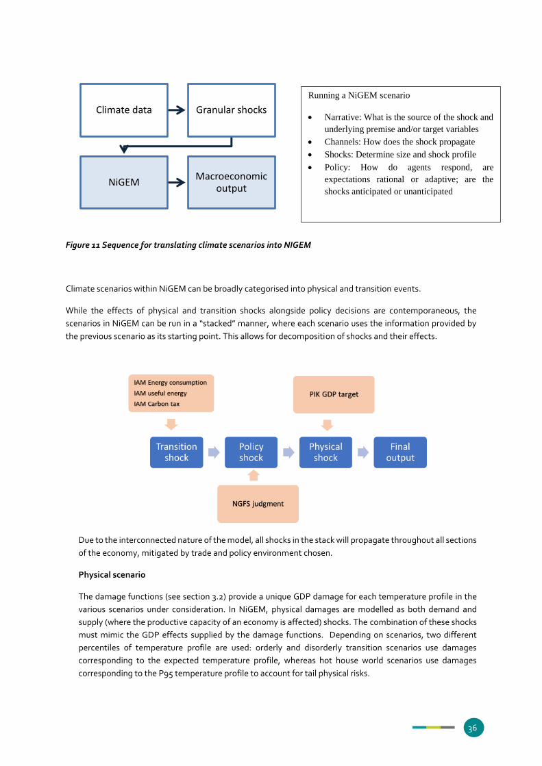
36

Figure 11 Sequence for translating climate scenarios into NIGEM

Climate scenarios within NiGEM can be broadly categorised into physical and transition events.

While the effects of physical and transition shocks alongside policy decisions are contemporaneous, the

scenarios in NiGEM can be run in a “stacked” manner, where each scenario uses the information provided by

the previous scenario as its starting point. This allows for decomposition of shocks and their effects.

Due to the interconnected nature of the model, all shocks in the stack will propagate throughout all sections

of the economy, mitigated by trade and policy environment chosen.

Physical scenario

The damage functions (see section 3.2) provide a unique GDP damage for each temperature profile in the

various scenarios under consideration. In NiGEM, physical damages are modelled as both demand and

supply (where the productive capacity of an economy is affected) shocks. The combination of these shocks

must mimic the GDP effects supplied by the damage functions. Depending on scenarios, two different

percentiles of temperature profile are used: orderly and disorderly transition scenarios use damages

corresponding to the expected temperature profile, whereas hot house world scenarios use damages

corresponding to the P95 temperature profile to account for tail physical risks.

Climate data Granular shocks

NiGEMMacroeconomic

output

Running a NiGEM scenario

Narrative: What is the source of the shock and

underlying premise and/or target variables

Channels: How does the shock propagate

Shocks: Determine size and shock profile

Policy: How do agents respond, are

expectations rational or adaptive; are the

shocks anticipated or unanticipated

37

Physical scenario policy environment

Adaptive expectations.

Interest rates and exchange rates are fixed.

Fiscal solvency is on.

Energy sector is exogenous.

As the physical shocks are intended to form part of a climate narrative with the transition shocks, policies

were chosen to isolate the physical effects from the transition. The physical shocks were based on

calibration to a target GDP damage rather than determining the GDP damage directly within NiGEM (as in

the transition shocks) so linkages within the model were reduced to their minimum trade links to ensure a

more direct coherence between the productivity shock used in the PIK methodology and the equivalent

NiGEM shocks used for calibration. In addition, with the exception of current policies, all energy effects are

captured by the transition shock so the energy sector is set exogenous to prevent double-counting.

Transition scenario inputs

It consists of:

Change in energy consumption and emissions under each scenario.

Change in “useful energy” (efficiencies) (see description at the end of section 3.1.4 Downscaling)

Carbon pricing.

Transition scenario channels

The shocks are primarily focused in three areas:

1. Prices

Carbon pricing will raise the price of energy, having an inflationary effect. This in turn will

reduce energy used in the economy, reducing production (without any additional efficiency

gains)

The reduction in fossil fuel usage due to carbon pricing will lead to a reduction in global (pre-

tax) fossil fuel prices leading to a deflationary effect.

2. Taxation

Carbon pricing will impose an additional tax on the economy, acting as a fiscal tightening

through a similar channel to VAT, leading to an inflationary effect.

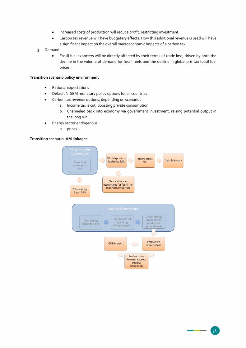
38

Increased costs of production will reduce profit, restricting investment.

Carbon tax revenue will have budgetary effects. How this additional revenue is used will have

a significant impact on the overall macroeconomic impacts of a carbon tax.

3. Demand

Fossil fuel exporters will be directly affected by their terms of trade loss, driven by both the

decline in the volume of demand for fossil fuels and the decline in global pre-tax fossil fuel

prices.

Transition scenario policy environment

Rational expectations

Default NiGEM monetary policy options for all countries

Carbon tax revenue options, depending on scenarios

a. Income tax is cut, boosting private consumption.

b. Channeled back into economy via government investment, raising potential output in

the long run.

Energy sector endogenous

o prices.

Transition scenario IAM linkages

IAM useful energy input

Total energy input declines

Partially offset by energy

efficiency gains

Useful energy available for production

generally falls

Productive capacity falls

GDP impact

In short-run demand exceeds

supply: inflationary

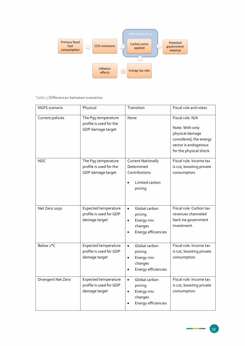
39

Table 5 Differences between scenarios

NGFS scenario Physical Transition Fiscal rule and notes

Current policies The P95 temperature

profile is used for the

GDP damage target

None Fiscal rule: N/A

Note: With only

physical damage

considered, the energy

sector is endogenous

for the physical shock.

NDC The P95 temperature

profile is used for the

GDP damage target

Current Nationally

Determined

Contributions

Limited carbon

pricing

Fiscal rule: Income tax

is cut, boosting private

consumption.

Net Zero 2050 Expected temperature

profile is used for GDP

damage target

Global carbon

pricing

Energy mix

changes

Energy efficiencies

Fiscal rule: Carbon tax

revenues channeled

back via government

investment.

Below 2°C Expected temperature

profile is used for GDP

damage target

Global carbon

pricing

Energy mix

changes

Energy efficiencies

Fiscal rule: Income tax

is cut, boosting private

consumption.

Divergent Net Zero Expected temperature

profile is used for GDP

damage target

Global carbon

pricing

Energy mix

changes

Energy efficiencies

Fiscal rule: Income tax

is cut, boosting private

consumption.

Potential government

revenue

IAM Carbon price

Primary fossil fuel

consumptionCO2 emissions

Carbon price applied

Energy tax rateInflation effects

40

Note: Additional

negative shock to

business confidence

Delayed transition Expected temperature

profile is used for GDP

damage target

Global carbon

pricing

Energy mix

changes

Energy efficiencies

Fiscal rule: Income tax

is cut, boosting private

consumption.

Note: Additional

negative shock to

business confidence

NiGEM output variables are the following:

General economic outputs

• Gross domestic product (GDP)

• Consumption, investment, government expenditure

• Technological innovation and capital productivity

• Unemployment rate

• Corporate profits, household income

• International trade flows

• Gross domestic income

• Trend capacity

• Energy prices and consumption

Specific economic outputs in the context of financial risk analysis

• Consumer price inflation

• Energy and commodity prices

• Interest rates

• Government bond yields

• Exchange rates between countries

• Equity market indices

• Real estate price indices (residential)

3.4. User manual for the NGFS Scenario Explorer

3.4.1. Data availability and license

The transition pathways selected for the NGFS are available in the NGFS Scenario Explorer (NGFS SE), hosted

by IIASA: data.ene.iiasa.ac.at/ngfs. The Scenario Explorer is a web-based user interface for scenario results and

historical reference data. It provides intuitive visualisations and display of time series data and download of the

data in multiple formats. A brief description of the features of the Scenario Explorer is available at the end of

this section and tutorial videos of the main features are available at https://software.ene.iiasa.ac.at/ixmp-

server/tutorials.html

The NGFS Scenario Explorer data are available under a Public License that is adapted from the Creative

Commons Attribution 4.0 International Public License with the aim of keeping the Licensed Material always up-

41

to-date and avoiding the circulation of obsolescent data constituting substantial portions of the Licensed

Material.

This license is a balance between making the scenario ensemble available as widely as possible, encouraging

broad use of the data for research, science communication and policy analysis and the anticipation of updates

of the scenario ensemble. This may be either due to adding more detailed information to available scenarios in

response to user requests, or because of reporting issues identified after the release that need to be corrected.

While we did take the utmost care to validate all submitted data, such issues can never be fully avoided.

For this reason, we request that downloads of scenario data are routed through the NGFS Scenario Explorer at

data.ene.iiasa.ac.at/ngfs, unless the data is made available in relation to a specific figure in a publication or

online visualisation tool, for example as supplementary material to a manuscript published in a scientific

journal.

We will inform registered users of the scenario ensemble about data updates or any other relevant news.

The details of the legal license are available under https://data.ene.iiasa.ac.at/ngfs/#/license

3.4.2. Data identifiers (Model, Scenario, Region, Variable)

The data from the NGFS Scenario Explorer are available for download in comma separated value (csv) format,

organised according to the IAMC data format. The numerical scenario results are provided as time series data.

Data is reported for each region and scenario available in the database, organised by variable with additional

columns for the available years. Hence, the columns in the data files are:

Model: The transition scenarios for the NGFS are provided by three integrated assessment models: GCAM 5.3,

MESSAGEix-GLOBIOM 1.1 and REMIND-MAgPIE 2.1-4.2. In the rest of this document, shorter versions of the

full model names are also used to refer to these three models; GCAM, MESSAGEix-GLOBIOM and REMIND-

MAgPIE, respectively.

The 2021 release of the NGFS scenarios includes two additional types of data sets:

It includes a subset of scenarios from a model version from REMIND-MAgPIE with integrated physical

damages. These are described in section 3.2.3 and are provided in the explorer with the model identifier

“REMIND-MAgPIE 2.1-4.2 IntegratedPhysicalDamages (median|95th)”, with median denoting the version in

which endogenous damages correspond to a median warming trajectory, and 95th to the version in which

warming corresponds to the 95th percentile.

Furthermore, the scenario data from NiGEM (see section 3.3) is provided under the model name “NiGEM NGFS

v1.21”.

Scenario: The scenario names are defined in line with Figure 1 on page 4 and Table 3 on page 17:

Hot house world: Current policies

Hot house world: Nationally determined contributions (NDCs)

Orderly: Below 2°C

Orderly: Net Zero 2050

Disorderly: Disorderly Transition

Disorderly: Divergent Net Zero

Model Scenario Region Variable Unit 2000 … 2100

42

The scenario names in the database come without the category (Hot house world, Orderly, Disorderly) to avoid too lengthy names. NiGEM takes input from each of the three standard IAM model versions, so that for each scenario narrative, there are three sets of scenario data from NiGEM. To differentiate these, the scenario names for NiGEM are appended with a suffix that indicates the IAM input of the respective scenario (e.g. “(with GCAM5.3_NGFS inputs)”). Region: The transition scenarios for the NGFS are provided for the native model regions as defined by each of the participating models and several aggregate regions (see below). The native model regions are labelled “MODEL NAME|REGION NAME” (e.g. “GCAM5.3_NGFS|Africa_Eastern”). The aggregated regions are labelled R5XXXX (e.g. R5ASIA), and individual countries are labelled by their ISO codes (e.g. CHN, IND, RUS, USA) with the exception of the European Union (EU). Global information is provided under “World”. Furthermore, downscaled data at the country level (see section 3.1.4) is available in a separate form, labelled “Country Name (downscaled)” or “D.ISO”. Variable: The variable names follow a few basic rules.

Variables are organized in a hierarchical structure which is specified by separators “|”

Variable names can include none, one or more separators (e.g. “Population”, “GDP|PPP”, “Emissions|CO2|Energy”)

For variables with one or more separators, the left-most word indicates a broad variable category or an indicator (e.g. “GDP”, “Emissions”, “Primary Energy”)

The separators define two types of relationships among variables: o Relationships for indicators calculated with different metrics or methods: e.g. “GDP|PPP” and

“GDP|MER” o Aggregate relationships providing disaggregation across sectors, fuels, technologies or gases:

e.g. “Emissions|CO2” = “Emissions|CO2|AFOLU” + “Emissions|CO2|Energy” + “Emissions|CO2|Industrial Processes”

Several alternatives may exist for aggregate relationships (e.g. Final Energy is decomposed by sector and by fuel)

Elements pertaining to the same hierarchical level can sometimes be aggregates themselves (e.g. “Primary Energy|Fossil” is the aggregate of “Primary Energy|Coal”, “Primary Energy|Oil” and “Primary Energy|Gas”)

Detailed description and definition of the variables in the database is available in Section 3.1.3, and can also be found on the Explorer on the “Documentation” tab. Unit: Each variable is specified by its unit, generally specified in the international system of units (SI units,

abbreviated from the French Système international (d'unités)).

3.4.3. Time steps and regional granularity

The time steps between two consecutive model output data range between 5 and 10 years and differ across the

participating models (Table ).

Table 6 Time steps across models

Model Time steps

GCAM 5-year time steps from 2005 to 2100

MESSAGEix-GLOBIOM 5-year time steps from 2005 to 2060 and 10-year timesteps over the period

2050-2100

REMIND-MAgPIE 5-year time steps from 2005 to 2060 and 10-year time steps over the

period 2050-2100

43

Regional granularity differs between the participating models. The MESSAGEix-GLOBIOM and REMIND-

MAgPIE models both have 11 model regions, whereas the GCAM model has 32 native model regions. The

regional definitions are summarised in Table A1.1, Table A1.2 and Table A1.3 for the individual models and Table

7 for the aggregate regions.

The downscaled data at the national level are available for each scenario under the regional category “Compare

(individual countries and regions)”. Within this category, countries that are modeled as native regions within

and IAM appear under their country name and countries whose results are derived from the downscaling tool,

appear under their name plus the extension “(downscaled)”. So, in order to see the results for e.g. the USA

across all three models, one should select both “United States of America” (for GCAM and REMIND-MAgPIE

this is a native model region) and “United States of America (downscaled)” (as it is part of the NAM region in

MESSAGEix-GLOBIOM).

In the downloadable files, the distinction between the native IAM model regions and the downscaled

information is made differently, namely in the model name. When the country information is derived from the

downscaling tool the model name is provided as MODEL_downscaled. When the country information is native

to the IAM model, the model name is simply provided as MODEL

Table 7 Regional definition of meta regions across models

NGFS SE identifier Geography name GCAM regions MESSAGEix-GLOBIOM regions REMIND-MAgPIE regions

BRA Brazil Brazil

CHN China China CPA CHA

EU European

Union

EU-12, EU-15 EEU, WEU EUR

IND India India SAS IND

USA United States USA NAM USA

JPN Japan Japan JPN

MEX Mexico Mexico

R5ASIA Asia Central Asia, China, India,

Indonesia, Pakistan, South

Asia, South Korea,

Southeast Asia, Taiwan

SAS, PAS, CPA CHA, IND, OAS

R5LAM Latin America Brazil, Central America and

Caribbean, Mexico, South

America_Northern, South

America_Southern,

Argentina, Colombia

LAM LAM

R5MAF Middle East

and Africa

Africa_Eastern,

Africa_Northern,

Africa_Southern,

Africa_Western, Middle

East, South Africa

MEA, AFR MEA, SSA

44

3.4.4. Meta-data

The following meta-data categories are available for grouped selection of scenarios.

The main scenario categories are:

Orderly

Disorderly

Hot house world

3.4.5. Scenario Explorer functionalities

The Scenario Explorer has been developed by IIASA and is increasingly used by the research community for

outreach and model comparison projects. For example, there are explorer instances accompanying the IPCC

SR1.5 and upcoming IPCC Sixth Assessment Report, and many projects funded by the Horizon 2020 EU

Research and Innovation programme (such as CD-LINKS www.cd-links.org), the Energy Foundation China,

GEIDCO and UNIDO make use of the explorer.

The transition scenarios selected for the NGFS are available in the NGFS Scenario Explorer hosted by IIASA:

data.ene.iiasa.ac.at/ngfs.

Tutorial videos of the main features are available at https://software.ene.iiasa.ac.at/ixmp-server/tutorials.html

New user registration

At the bottom of the login box at the landing page of the explorer there is a registration button which will open

the new user registration page. Once you fill out this form, at least providing username, email and password,

you will receive an email to confirm your registration and you will have access to the NGFS Scenario Explorer.

If you are already registered for one of the other Scenario Explorer instances (such as the IPCC SR1.5), there is

no need to register again. Your account should work on the NGFS Scenario Explorer as well. For any questions,

please email ngfs.ene.admin@iiasa.ac.at.

It is also possible to use the NGFS Scenario Explorer without registration. In that case, simply click the Guest

Login button at the landing page to enter the NGFS Scenario Explorer. When using the Scenario Explorer

without registration, it is possible to use all the features of the Scenarios Explorer, but without the possibility

so save and share workspaces.

Workspaces

The Scenario Explorer is built around the concept of workspaces, which can be developed, saved and shared

between users. Workspaces are interactive, user-customisable environments that can contain charts, data-

tables and text descriptions. Any registered user of the Scenario Explorer can create, save and share

R5OECD90+EU OECD and EU USA, Australia_NZ,

Canada, EU-15,

Europe_Non_EU, European

Free Trade Association,

Japan

WEU, PAO, NAM, EEU EUR, JPN, USA, CAZ, NEU

R5REF Reform

economies

EU-12, Europe_Eastern,

Russia

FSU REF

45

workspaces. Workspaces can be generated to be public such that every user sees them when accessing the

Scenario Explorer instance or they can be shared bilaterally with colleagues or on social-media.

To create a new workspace, click the ‘create workspace’ button at the top of the Scenario Explorer page. This

will create and open a new workspace for you. By clicking on ‘edit workspace’ the workspace setting page will

be opened, allowing to provide a name and description of the workspace and to save the workspace to the

server. The three-striped workspace menu on the top-right provides the option to export the workspace code

in json file format, to export the workspace as pdf or to clone the workspace. Cloning the workspace will create

a copy that can be edited without interfering with the original version. It is possible to clone workspaces that

have been shared by other users or to clone workspaces that are already saved to your account. Updating the

workspace will reload it from the server and overwrite any changes that have been made locally.

Finally, the workspace setting page allows to reorder the panels in the workspace.

Panels

Any charts, data-tables and text descriptions within a workspace are called ‘panels’. New panels can be created

with the ‘plus’ button, or by clicking ‘create a new timeseries panel’ at the top of the page.

The first step in creating a new data or figure panel is to select scenarios, either from a set of meta-

characterisations of the scenarios or by selecting individual scenarios from the full list.

The second step is selection of the variables, either by categories or from selecting individual variables from the

full list. It is possible to scroll through the full list, or to search variables by typing part of the variable name in

the search box.

The third step is the selection of regions. The default region is ‘world’, but any of the above-described regions

can be selected.

After these selection steps, the plot can be created by clicking the ‘apply’ button.

After creating the graph, the following features are available:

Adjusting the ranges shown on the graph, in the ‘ranges’ tab

Change the title and add a description under the ‘options’ tab (and click update after changing title or

description)

The filter panel can be hidden and reopened by clicking on the above-pointing arrow in the top bar of

the panel.

The legend can be shown or hidden with the most left button in the top bar of the panel

The figure can be converted to line chart, bar chart of data table by clicking the respective buttons in

the top bar

Sub-categories can be shown in stacked format as well.

The data underlying the panel can be downloaded in several different data formats (such as xlsx, csv)

or the figure itself can be downloaded as pdf or other picture format.

The size of the panel can be adjusted from full-width to half-width using the minimise panel button.

When a workspace contains multiple panels, the chain-button in the top of the workspace allows to cross-

highlight the same scenario across multiple panels for easy comparison.

Finally, creating a text panel allows to add text descriptions to a workspace with formatting based on the

markdown language.

46

Documentation

Documentation is provided at the level of individual panels (using the document-icon) or for the full database

in the documentation menu at the top of the Scenario Explorer. Definitions and links to more detailed

documentation and references are provided for all models, scenarios, variables, regions and metadata

categories that are used for scenario categorisation.

Download features

The data of an individual panel can be downloaded in several different data formats (such as xlsx, csv) or the

figure itself can be downloaded as pdf or other picture format.

The data contained in the full database can be downloaded through the download menu at the top of the

Scenario Explorer. This menu contains snapshots in csv format for all scenarios and variables in the database,

the reference data and citation options for the data in different formats. There are separate files for

downloading the IAM model data and the downscaled national level data.

47

4. Climate Impact Explorer and data

4.1. Introduction to the Climate Impact Explorer

The Climate Impact Explorer (CIE) provides first-hand access to projections of physical climate risks at the

continental, national and subnational level. It shows maps and graphs illustrating the projected changes in

climate conditions, resulting impacts and damages on selected sectors for several global warming levels, and

also how they will play out over time according to various policy-relevant emission scenarios (including those

from the Network for Greening the Financial System, or NGFS). All display materials and the underlying data

can be downloaded through the CIE interface.

The key functionalities of the Climate Impact Explorer are the following:

Projections of climate impacts at the national and subnational level on annual and seasonal scales:

o Including uncertainty ranges encompassing both the global climate sensitivity to emissions and

the response of local impacts to global warming

o Aggregation at the continental, national and subnational levels using weighted averages by either

area, GDP, or population

Time evolution of future impacts for several policy-relevant scenarios from the NGFS, the Climate

Action Tracker and for the Representative Concentration Pathways

Country maps for different warming levels containing information on the robustness of the

projections, based on the agreement between the various climate and impact models used to derive

them (model agreement)

Climate and climate impact indicators covering several biophysical sectors and economic damages

from selected extreme events

The possibility to download all displayed graphs and maps, as well as the data underlying them

As a guidance note for users, the Climate Impact Explorer provides a comprehensive, globally consistent

dataset of physical risk projections for different climate scenarios. The use of global datasets means regional

representations are not consistently evaluated and can show deviations from other datasets used in risk

assessments focused on the regional, national or subnational level. The findings from the Climate Impact

Explorer should thus be used to supplement rather than replace national or regional risk assessments.

4.2. Methodology behind the Climate Impact Explorer

4.2.1. Core Concept and overview of the modelling chain

The Climate Impact Explorer is meant to provide information about projected changes in various climate impact indicators for several levels of global warming, and how they may unfold over time according to various scenarios of greenhouse gas emissions. This information is provided at the country level, both in the format of time series with 5-year time steps until 2100 and as maps visualizing projected changes for distinctive global warming levels (1.5°C, 2°C, 2.5°C, and 3°C). The information is derived from an ensemble of climate and climate impact models that participated in international model intercomparison initiatives. The aim of the tool is to show climate impact outcomes for different emissions scenarios, also providing the associated full uncertainty ranges across global warming.

48

Figure 12 Flowchart illustrating the whole methodological sequence that was used to produce the

visualisations shown on the Climate Impact Explorer.

The emissions scenarios for which we visualise projected impacts were derived with Integrated Assessment Models (IAMs) and either produced by the Climate Action Tracker, developed by academic institutions as part of a collaboration with the Network for Greening the Financial System, or are classically used in climate science research (the Representative Concentration Pathways). Some basic information on those scenarios is provided in Section 4.2, we refer to the institutions that derived them for further details including on the characteristics of IAMs. In this Section 4.1, we provide information on the subsequent methodological steps (see also Fig. 13):

1) The MAGICC6 simple climate model is used to capture the full Global Mean Temperature (GMT) uncertainty for different emissions scenarios. The data is available from the NGFS Scenario Explorer hosted by IIASA.

2) Impact projections are assessed for time slices centred around various global warming levels in the

global, open access databases produced by the Inter-Sectoral Impact Model Intercomparison Project (ISIMIP) and the CLIMADA model. They are averaged from the simulation results of several scenario experiments, each conducted with a number of climate and climate impact models, thereby making use of the full information available in the Inter-Sectoral Impact Model Intercomparison Project (ISIMIP) archive. This allows us to ascribe these projections to any greenhouse gas emission scenario for which GMT trajectories are available, including the NGFS scenarios.

3) Uncertainty ranges across the climate model / impact model ensemble from ISIMIP are derived by

quantifying the distribution of the results from the various model combinations or by applying a quantile regression on those.

The rest of this Section 4.1 provides more details on the data processing procedure, including these three key methodological steps. The emission scenarios displayed in the Climate Impact Explorer, the ISIMIP database, the models that contributed to it, as well as the CLIMADA model are described in Section 4.2. Section 4.3 focuses on the visualisations shown on the Climate Impact Explorer.

49

Figure 13 Illustration of the various sources of uncertainty in the climate impact chain (see coloured squares at the bottom), and the 3 key methodological steps applied to account for those in the projections shown by the Climate Impact Explorer.

4.2.2. Global Mean Temperature (GMT) Projections

The CIE shows impact projections corresponding to various greenhouse gas emission pathways used by the

NGFS or assessed by the Climate Action Tracker (CAT), or classically used in climate science research (the

Representative Concentration Pathways, or RCPs). These pathways were derived either by Integrated

Assessment Models (IAMs, in the case of the NGFS scenarios and the RCPs), or by policy analysis (in the case of

the CAT scenarios). Then, the Model for the Assessment of Greenhouse-gas Induced Climate Change

(MAGICC6, Meinshausen et al., 2011) – a reduced-complexity climate model – was used to simulate the

resulting GMT trajectories.

MAGICC6 applies a probabilistic modelling approach to capture the range of uncertainty in the GMT response

to a given emissions trajectory (determined by the climate sensitivity, see here) by considering 600 different

parameterizations. In the CIE, we display the uncertainty in global mean temperature projections through the

5-95% range from the MAGICC6 realisations (Fig. 14). Neither the greenhouse gas emission scenarios included

in the CIE nor the resulting GMT trajectories derived with MAGICC6 were prepared by the contributors to the

CIE; for further details on those we encourage consulting the corresponding references added in this paragraph

or elsewhere in the documentation.

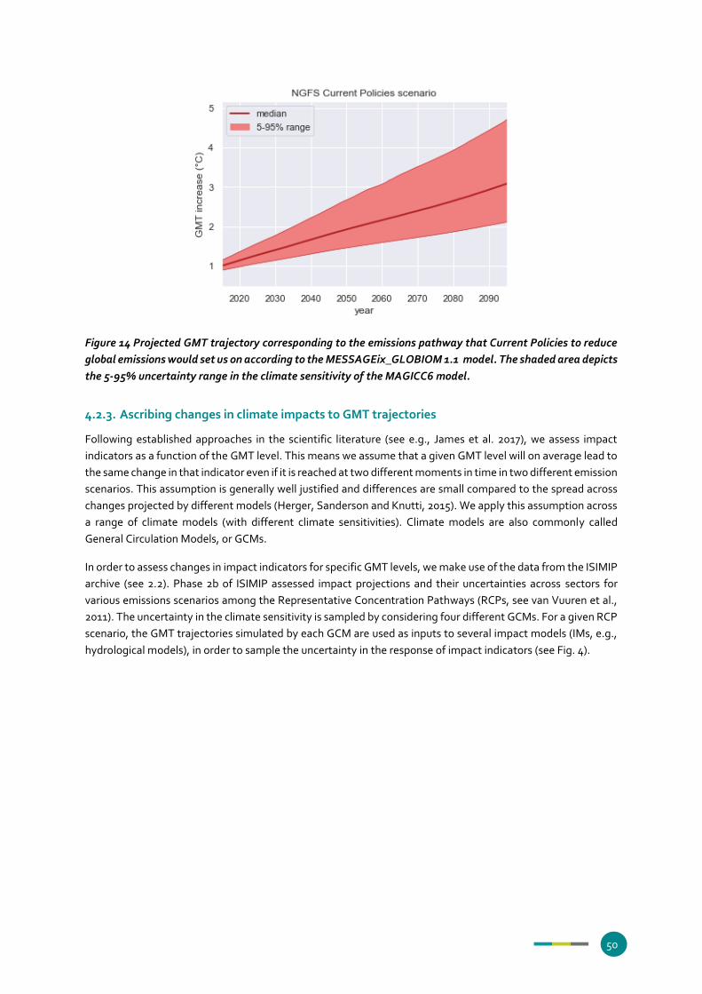
50

Figure 14 Projected GMT trajectory corresponding to the emissions pathway that Current Policies to reduce

global emissions would set us on according to the MESSAGEix_GLOBIOM 1.1 model. The shaded area depicts

the 5-95% uncertainty range in the climate sensitivity of the MAGICC6 model.

4.2.3. Ascribing changes in climate impacts to GMT trajectories

Following established approaches in the scientific literature (see e.g., James et al. 2017), we assess impact

indicators as a function of the GMT level. This means we assume that a given GMT level will on average lead to

the same change in that indicator even if it is reached at two different moments in time in two different emission

scenarios. This assumption is generally well justified and differences are small compared to the spread across

changes projected by different models (Herger, Sanderson and Knutti, 2015). We apply this assumption across

a range of climate models (with different climate sensitivities). Climate models are also commonly called

General Circulation Models, or GCMs.

In order to assess changes in impact indicators for specific GMT levels, we make use of the data from the ISIMIP

archive (see 2.2). Phase 2b of ISIMIP assessed impact projections and their uncertainties across sectors for

various emissions scenarios among the Representative Concentration Pathways (RCPs, see van Vuuren et al.,

2011). The uncertainty in the climate sensitivity is sampled by considering four different GCMs. For a given RCP

scenario, the GMT trajectories simulated by each GCM are used as inputs to several impact models (IMs, e.g.,

hydrological models), in order to sample the uncertainty in the response of impact indicators (see Fig. 4).

51

Figure 15 Schematic representation of the increase in an impact indicator for a given scenario. Two GCMs

(represented by the red and blue colours) are used to sample uncertainty in the climate sensitivity. Several

IMs are then used to assess uncertainty in the impact response to a given GMT trajectory (visualised by the

envelopes constituted by the dashed lines). A similar change in a given impact indicator can be expected for

a given GMT level reached at a different moment in time by the two different GCMs. Looking at the median

of the impact for the two GCMs gives more confidence on its actual value, while the dispersion across the

results of each IM simulation for this GMT indicates the full uncertainty (in the climate and impact response).

In our case, we have results for several RCP simulation runs (by default RCP2.6 and RCP6.0, as well as RCP8.5

and RCP4.5 for some indicators). In each GCM simulation corresponding to each RCP scenario (a scenario-GCM

combination), we identify the year for which a certain GMT level is reached (using a running mean over a 21-

year period, see Table 1). We do so for all GMT levels attained in the available scenario-GCM combinations,

starting with 1°C and with a 0.1°C increment (that is to say: 1°C, 1.1°C, etc.). Under the current rate of warming

(~0.2°C per decade), this increment corresponds to about 5 years of global warming.

Table 8: Years when the Warming Levels between 1.0 and 3.4°C are reached in the considered scenario-

GCM combinations.

Warmi

ng

Level

[C°]

GFDL-

ESM2

M

rcp26

GFDL-

ESM2

M

rcp45

GFDL-

ESM2

M

rcp60

GFDL-

ESM2

M

rcp85

HadG

EM2-

ES

rcp26

HadG

EM2-

ES

rcp45

HadG

EM2-

ES

rcp60

HadG

EM2-

ES

rcp85

IPSL-

CM5A

R

rcp26

IPSL-

CM5A-

LR

rcp45

IPSL-

CM5A-

LR

rcp60

IPSL-

CM5A-

LR

rcp85

MIRO

C5

rcp26

MIRO

C5

rcp45

MIRO

C5

rcp60

MIRO

C5

rcp85

1.0 2015 2015 2017 2016 2007 2007 2006 2006 2008 2011 2010 2008 2012 2013 2015 2012

1.1 2021 2021 2025 2022 2010 2010 2009 2009 2013 2016 2014 2013 2018 2018 2024 2015

1.2 2030 2028 2032 2027 2012 2013 2012 2011 2016 2019 2018 2016 2025 2023 2032 2019

1.3 2079 2034 2045 2031 2014 2016 2015 2013 2020 2023 2022 2020 2030 2028 2038 2023

1.4 2100 2043 2053 2035 2016 2019 2017 2015 2024 2026 2025 2023 2036 2033 2043 2027

1.5 2051 2059 2038 2019 2023 2022 2018 2030 2029 2030 2025 2042 2035 2048 2031

1.6 2058 2062 2041 2022 2026 2026 2021 2036 2032 2035 2028 2047 2040 2053 2033

1.7 2065 2065 2044 2025 2030 2030 2024 2045 2035 2038 2031 2092 2045 2058 2037

1.8 2079 2068 2047 2027 2033 2034 2026 2062 2038 2042 2033 2051 2062 2042

1.9 2092 2072 2050 2036 2036 2037 2029 2041 2045 2035 2057 2066 2044

2.0 2076 2053 2041 2038 2042 2031 2044 2048 2037 2063 2069 2047

52

2.1 2081 2057 2050 2042 2045 2034 2048 2052 2039 2073 2071 2049

2.2 2086 2060 2045 2049 2036 2052 2056 2040 2079 2075 2051

2.3 2093 2063 2048 2052 2039 2055 2061 2043 2095 2078 2054

2.4 2097 2066 2050 2055 2040 2060 2065 2044 2097 2081 2056

2.5 2069 2053 2057 2042 2067 2070 2046 2086 2058

2.6 2071 2057 2060 2044 2072 2073 2048 2091 2061

2.7 2074 2061 2062 2046 2087 2077 2050 2091 2062

2.8 2077 2063 2064 2048 2095 2080 2052 2091 2065

2.9 2081 2067 2067 2050 2106 2083 2054 2091 2067

3.0 2083 2070 2069 2052 2150 2086 2056 2069

3.1 2086 2075 2071 2053 2161 2089 2058 2072

3.2 2088 2105 2073 2055 2203 2060 2074

3.3 2092 2117 2076 2057 2240 2061 2076

3.4 2093 2156 2080 2058 2256 2063 2079

Projected changes in the indicators shown on the Climate Impact Explorer are always expressed as absolute or

relative differences compared to the values in the 1986-2006 reference period (for the indicators derived from

ISIMIP data, see 2.2) or in the reference year 2020 (for the indicators derived from CLIMADA data, see 2.3).

These changes were simulated in scenario experiments conducted either by GCMs or IMs (using GCMs outputs

as input data). After identifying the year for which a specific GMT level is reached in a scenario-GCM

combination, for each indicator we average the projected values over the 21-year period centred over that year

in the corresponding GCM or IM scenario experiment. We then average over all available scenarios for each

GCM or GCM-IM combination, before pooling the estimates obtained from all GCMs or GCM-IM combinations,

from which we compute their median values for each GMT level.

With these estimates of changes in impact indicators for each GMT level of interest, we can derive impact

projections for any scenario that reaches these levels. To that end, we identify the points in time when these

specific GMT levels are reached and ascribe to them the change in impact indicator computed in the previous

step.

It is important to note that our confidence in the results decreases for high warming levels (and particularly

beyond 2.5-3°C of global warming), since these levels have been attained in a smaller number of the RCP

experiments due to the differing climate sensitivity of the GCMs that conducted them.

4.2.4. Impact projection uncertainties

The uncertainty in impact projections is estimated from the spread in the projections from all GCMs (for climate

indicators) or GCM-IM combinations (for sectoral impact indicators), over the GMT levels that are attained by

all GCMs in the RCP experiments available for the considered indicator (see 1.3), starting with 1°C of global

warming and with an increment of 0.1°C. We calculate deviations of GCM-IM projections to their ensemble

median and apply a quantile regression to these deviations. As a result, we obtain the relationships between

the 5th and 95th percentiles of impact projections and the global warming levels (Fig. 5). A consistency check

is applied with regard to the regression estimates for the 5th or 95th percentiles. Specifically, issues can arise

when extrapolating linear quantile regressions to high warming levels for which limited data are available. In

53

case of unrealistic regression outcomes (i.e. crossing of the zero line), we compute the corresponding percentile

(5th or 95th) after having pooled impact projections for all GMT levels reached by all GCMs in the available RCP

experiments, and consider that its difference to the ensemble median remains constant with global warming.

Figure 16 Deviations in area-weighted average annual near surface air temperature from the ensemble

median of all GCMs, for each warming level (x-axis). The blue and orange lines show the quantile regression

lines for the 5th and 95th percentiles. Provided that they don’t cross the x-axis between 1° and 5°C, these

two lines are used to quantify the impact uncertainty at each warming level.

4.2.5. Estimation of the full uncertainty range

The full uncertainty range displayed is the combination of the uncertainty in the GMT response to a given

emission scenario (or climate sensitivity, see 1.2) and in the response of the indicator of interest to a given GMT

trajectory (assessed following the methodology described in 1.4). The 5-95% uncertainty ranges characterizing

each source of uncertainty are then combined to provide the full uncertainty range. An example is provided in

Fig. 6, with the 5-95% MAGICC6 uncertainty for GMT projections highlighted in green and the 5-95%

uncertainty for impact projections in brown. The combined full uncertainty range is given by the blue markers.

54

This approach assumes independence of the local response of climate or impact indicators from the global

climate sensitivity. While this is generally a justifiable assumption, there might be specific regions and impacts

for which global sensitivities and regional changes in impact indicators are coupled.

Figure 17 Illustration of the combined uncertainties in the global mean temperature and local impact

response, in the case of near-surface air temperature changes in Germany.

4.2.6. Additional data processing steps

4.2.6.1. Masking of grid cells for specific variables

For surface runoff, model grid cells exhibiting a mean value of less than 0.05 mm/day in the reference period

are masked in the displayed maps and excluded for the computation of national and subnational averages. This

mask is computed separately for each season and the annual mean (see 1.6.2). The mask that was hereby

derived from annual mean runoff values is also applied to discharge as well as maximum and minimum of daily

river discharge. For these variables, this masking is thus not dependent on the season.

4.2.6.2. Temporal averages

For most impact indicators, changes in annual mean as well as seasonal mean values were calculated. The

considered seasons were: December-January-February, March-April-May, June-July-August, and September-

October-November.

4.2.6.3. National or subnational level averages

Four different spatial aggregation methods have been used to derive the time series that can be visualised in

the CIE.

For many indicators, the user can choose between three spatial weighted averaging methods: by area,

population or GDP. To derive area-weighted averages, each grid cell is weighted by the fraction of the land area

of the selected territorial unit it covers. For population weighted averages, each grid cell is weighted by the

fraction of the population of the selected territorial unit located in the grid cell. For grid cells that do not fully

lie within a territorial unit, the population of the grid cell is scaled to the fraction of the grid cell that is covered

55

by this territory. GDP-weighting is computed in a similar way as for population, but uses information on the

repartition of the GDP across a territorial unit. We use the gridded population and GDP data corresponding to

year 2005 provided by ISIMIP, assuming that the repartition of population and GDP within a country will stay

constant in the future. The indicators land fraction or population annually exposed to a certain category of

extreme events (see 2.2) were originally derived by using one of these averaging methods (area-weighted or

population-weighted, respectively), therefore only one corresponding option can be selected for these

indicators.

The indicators quantifying economic damages derived from CLIMADA (see 2.3) were calculated using a

different spatial aggregation method: The locally estimated damages were summed over the grid cells of

interest. Therefore, only the option “sum” can be selected in the drop-down menu for these indicators.

4.2.6.4. Smoothing of time series

Although the projected changes in impact indicators for a specific GMT level are extracted from 21-year

averages for each scenario-GCM or scenario-GCM-IM combination (the full procedure is detailed in 1.3), they

can still be subject to internal climate variability. Before showing them on the Climate Impact Explorer, we

therefore perform an additional smoothing of the calculated time series by conducting a running average of

the projected changes over three consecutive warming levels (meaning, over a window of a 0.3°C size). This

smoothing is applied on the median as well as the upper and lower bounds of the projected changes.

4.3. Models, scenarios and data sources

4.3.1. Emission scenarios

In the Climate Impact Explorer, we provide time series plots illustrating how climate impacts may unfold over

time according to various scenarios of greenhouse gas emissions. These scenarios were derived with Integrated

Assessment Models (IAMs) and either produced by the Climate Action Tracker, developed by academic

institutions as part of a collaboration with the Network for Greening the Financial System, or are classically

used in climate science research (the Representative Concentration Pathways).

4.3.2. NGFS Scenarios

The CIE displays climate impacts on biophysical systems, extreme events and resulting economic damages for

three of the six NGFS scenarios:

1) Net-Zero 2050 is an ambitious scenario that limits global warming to 1.5°C through stringent

climate policies and innovation, reaching net zero CO2 emissions around 2050. This scenario is thus

compatible with the long-term temperature goal of the Paris Agreement.

2) Delayed transition assumes annual emissions do not decrease until 2030. Strong policies are then

needed to limit warming to below 2°C.

3) Current Policies assumes that only currently implemented policies are preserved, leading to a

global warming by up to 3°C by 2100 and high associated climate impacts.

The derivation of the GMT trajectories resulting from these scenarios was done using MAGICC6 (see Section

1.2). More information on these scenarios is available on the NGFS Scenarios Portal or the NGFS IIASA Scenario

Explorer.

56

4.3.3. Representative Concentration Pathways

The Representative Concentration Pathways (RCPs) are greenhouse gas concentration scenarios that are

commonly used in the climate modelling community. Produced within CMIP5, they were officially adopted by

the Intergovernmental Panel on Climate Change (IPCC) and provide a basis for the projections and predictions

of the Fifth Assessment Report of the IPCC. The RCPs are defined by the approximate level of radiative forcing

(in W/m2) by the end of the 21st century relative to the pre-industrial level. The use of radiative forcing allows

the calibration of different warming potentials of various greenhouse gases. The word “representative”

signifies that each pathway is an archetype of several scenarios sharing similar radiative forcing and emission

characteristics.

The set of RCPs included in the CIE were designed such that they are representative of all available scenarios at

the time of their development. It consists of four harmonious but distinguishable pathways, each of them

offering a plausible and internally consistent description of the future: RCP2.6 that leads to a low level of forcing

compatible with a GMT increase by less than 2°C by 2100, two intermediate stabilization scenarios, RCP4.5 and

RCP 6.0, and a high emission pathway, RCP8.5. They are driven by various assumptions about population, GDP,

energy use and mix, and land-use and thus carry substantial uncertainties. van Vuuren et al. (2011) provide more

details on the main characteristics of these four RCPs, such as emission trends and end-century warming levels

(which were assessed using MAGICC, see section 1.2).

4.3.4. Scenarios from the Climate Action Tracker

The Climate Action Tracker is an independent scientific analysis that tracks government climate action and

measures it against the globally agreed Paris Agreement aim of "holding warming well below 2°C, and pursuing

efforts to limit warming to 1.5°C." A collaboration of two organisations, Climate Analytics and New Climate

Institute, the CAT has been providing this independent analysis to policymakers since 2009.

CAT quantifies and evaluates climate change mitigation commitments from all the biggest emitters and a

representative sample of smaller emitters covering about 80% of global emissions and approximately 70% of

global population. It then assesses whether countries are on track to meeting those commitments. More

precisely, in the CIE we show projected impacts for an emission scenario called Current Policies, reflecting the

projected effect of the policies that governments in the analysed countries have implemented or enacted and

how these are likely to affect national emission over the time period to 2030, and where possible beyond.

CAT then aggregates country action to the global level, determining a likely GMT trajectory by the end of the

century, as well as the associated uncertainty range, using MAGICC6 (see section 4.1.2).

4.3.5. ISIMIP Data

The Inter-Sectoral Impact Model Intercomparison Project (ISIMIP) is a community-driven initiative with the aim

of offering a consistent climate change impact modelling framework. By early 2021, more than 100 models had

contributed to the initiative. The participating impact models are listed on the ISIMIP website where a factsheet

is provided for each model. To participate, impact modelling teams agree to run a minimal set of model

experiments. These include scenario experiments which simulate the evolution of sectoral impact variables

until at least 2100 under specific trajectories in terms of climate and socio-economic forcings, for which they

are provided with the corresponding input data. The resulting output data become open access after an

embargo period and can be downloaded from https://data.isimip.org. On the Climate Impact Explorer, we show

input (Table 2) and output data (Table 3 and 4) from phase 2b of ISIMIP (ISIMIP2b), available at a spatial

resolution of 0.5° (equivalent to ~50km at the equator, and further reducing as one moves poleward). This

spatial resolution has to be kept in mind when interpreting the graphs and maps displayed on the Climate

Impact Explorer, especially over small areas such as small island states.

57

The ISIMIP2b climate input data were obtained with 4 GCMs from the fifth phase of the Coupled Model

Intercomparison Project (CMIP5). They have been bias-adjusted, meaning that biases between the values

simulated by each GCM and those from an observation-based reference dataset over a common period have

been corrected, and that this correction has been applied to the whole period simulated by the GCMs (assuming

that the identified biases stay constant over time). The reference dataset used for the bias adjustment is

EWEMBI (E2OBS, WFDEI and ERA-Interim data merged and bias-corrected for ISIMIP; see Lange et al., 2019),

which covers the 1979-2005 period. The correction was done independently for each variable, grid cell and

month. The bias adjustment was performed on the regular 0.5° grid from EWEMBI, onto which the CMIP5 GCM

data were interpolated (Frieler et al., 2017; Lange, 2018). It is important to note that the bias-adjustment

technique employed for ISIMIP preserves the indicators trends displayed in the Climate Impact Explorer. More

detailed information on the methodology can be found in the ISIMIP2b bias-correction fact sheet under

www.isimip.org/gettingstarted/isimip2b-bias-correction/.

Unlike the climate indicators, the sectoral impact indicators displayed on the Climate Impact Explorer did not

undergo a bias-adjustment or validation procedure. While such a validation would be highly desirable, it is

generally challenging for sectoral climate impacts on the global level due to a lack of data both on the

biophysical quantities as well as on other human interventions (e.g. dikes for flood protection, forest

management, or groundwater extraction for irrigation).

Although country-level information is provided, it does not mean that the results of each impact model have

been evaluated and validated for each country. Importantly, the Climate Impact Explorer delivers information

on the sole effects of climate change according to the available indicators derived from ISIMIP, while assuming

constant socio-economic conditions (such as population, GDP, water use, etc.). In reality, socio-economic

development will strongly affect future impacts.

Table 9: Bias-corrected climate variables used as input for ISIMIP

Bias-Corrected Climate Variables

Variable Name Abbreviation Unit Unit longname Temporal

Resolution/Aggregation

Output

metrics

Relative Humidity hursAdjust % percent daily --> mean

Relative humidity is defined as the ratio of water vapour in the air to the total amount that could be held at its current temperature (saturation

level). Here we consider relative humidity at 2 metres above ground. The data used for this variable have undergone a bias-adjustment

procedure to correct for deviations between modelled and observed values over the time period where they overlap.

Specific Humidity hussAdjust kg kg-1 kilogram per kilogram daily --> mean relative

Specific humidity is defined as the mass of water vapour contained in each kg of air. Here we consider specific humidity at 2 metres above

ground. The data used for this variable have undergone a bias-adjustment procedure to correct for deviations between modelled and

observed values over the time period where they overlap.

Precipitation prAdjust kg m-2 s-1 kilogram per square metre per

second

daily --> sum relative

Precipitation is defined as the mass of water (both rainfall and snowfall) falling on the Earth's surface, per unit area and time. The data used

for this variable have undergone a bias-adjustment procedure to correct for deviations between modelled and observed values over the time

period where they overlap.

Snowfall prsnAdjust kg m-2 s-1 kilogram per square metre per

second

daily --> sum relative

58

Snowfall is defined as the mass of water falling on the Earth's surface in the form of snow, per unit area and time. The data used for this

variable have undergone a bias-adjustment procedure to correct for deviations between modelled and observed values over the time period

where they overlap.

Atmospheric Pressure

(surface)

psAdjust Pa Pascal daily --> mean absolute

Atmospheric pressure quantifies the force exerted by the weight of the column of air situated above a given location, per unit area. Here we

consider atmospheric pressure at 2 metres above ground. The data used for this variable have undergone a bias-adjustment procedure to

correct for deviations between modelled and observed values over the time period where they overlap.

Atmospheric pressure

(adjusted to sea level)

pslAdjust Pa Pascal daily --> mean absolute

Atmospheric pressure quantifies the force that would be exerted by the weight of the column of air situated above a given location, per unit

area. Since atmospheric pressure decreases with altitude, here we inspect the atmospheric pressure at 2 metres above ground but adjusted as

if the location of interest was set at sea level. This allows comparison of locations situated at different altitudes. The data used for this

variable have undergone a bias-adjustment procedure to correct for deviations between modelled and observed values over the time period

where they overlap.

Downwelling Longwave

Radiation

rldsAdjust W m-2 Watt per square metre daily --> mean relative

Downwelling longwave radiation is defined as the downward energy flux in the form of infrared light that reaches the Earth's surface. The

data used for this variable have undergone a bias-adjustment procedure to correct for deviations between modelled and observed values over

the time period where they overlap.

Wind Speed sfcWindAdjust m s-1 metre per second daily --> mean relative

Wind speed quantifies the velocity of an air mass. Here we consider the wind speed 10 metres above ground. The data used for this variable

have undergone a bias-adjustment procedure to correct for deviations between modelled and observed values over the time period where

they overlap.

Air Temperature tasAdjust °C degrees Celsius daily --> mean absolute

Air temperature refers to the temperature of air masses near the Earth's surface (2 metres above the ground in this case). The data used for

this variable have undergone a bias-adjustment procedure to correct for deviations between modelled and observed values over the time

period where they overlap.

Daily Maximum Air

Temperature

tasmaxAdjust °C degrees Celsius daily --> mean absolute

Daily maximum air temperature is defined as the peak air temperature reached in a day, in this case at 2 metres above the ground. The data

used for this variable have undergone a bias-adjustment procedure to correct for deviations between modelled and observed values over the

time period where they overlap.

Daily Minimum Air

Temperature

tasminAdjust °C degrees Celsius daily --> mean absolute

Daily minimum air temperature is defined as the lowest air temperature reached in a day, in this case at 2 metres above the ground. The data

used for this variable have undergone a bias-adjustment procedure to correct for deviations between modelled and observed values over the

time period where they overlap.

Table 10: ISIMIP Primary Output Variables

ISIMIP Primary Output Variables

Snow Depth snd m metre monthly -->

mean

relative

59

Snow depth is defined as the thickness of the snow layer covering the ground. [5 impact models]

Surface Runoff qs kg m-2 s-1 kilogram per square metre per

second

monthly -->

mean

relative

Surface runoff (also called overland flow) describes the flow of water occurring on the Earth's surface when excess water, e.g. rainwater, can no

longer be absorbed by the soil. [12 impact models]

River Discharge dis m3 s-1 cubic metres per second daily --> mean relative

Discharge (also called streamflow) is the volume of water flowing through a river or stream channel. [15 impact models]

Maximum of Daily River

Discharge

maxdis m3 s-1 cubic metres per second monthly --> max relative

Maximum of daily discharge is defined as the peak volume of water flowing through a river or stream channel in a day. [2 impact models]

Minimum of Daily River

Discharge

mindis m3 s-1 cubic meters per second monthly --> min relative

Minimum of daily discharge is defined as the lowest volume of water flowing through a river or stream channel in a day. [2 impact models]

Soil Moisture soilmoist kg m-2 kilogram per square metre monthly -->

mean

relative

Total soil moisture content quantifies water stored in soil, per unit area. Here we consider soil moisture contained within the root zone, i.e. until a

depth of approximately 1 metre. [15 impact models]

Maize Yields yield_maize t ha-1 (dry

matter)

tons of dry matter per hectare per growing

season

relative

Maize yields were calculated by assuming that the cultivated areas of both rainfed and irrigated maize will remain constant through the 21st

century. Their projected changes hence only reflect the future evolution of climate, and not that of agricultural management practices. [4 impact

models]

Rice Yields yield_rice t ha-1 (dry

matter)

tons of dry matter per hectare per growing

season

relative

Rice yields were calculated by assuming that cultivated areas of both rainfed and irrigated rice will remain constant through the 21st century. Their

projected changes hence only reflect the future evolution of climate, and not that of agricultural management practices. [4 impact models]

Soy Yields yield_soy t ha-1 (dry

matter)

tons of dry matter per hectare per growing

season

relative

Soy yields were calculated by assuming that the cultivated areas of both rainfed and irrigated soy will remain constant through the 21st century.

Their projected changes hence only reflect the future evolution of climate, and not that of agricultural management practices. [4 impact models]

Wheat Yields yield_wheat t ha-1 (dry

matter)

tons of dry matter per hectare per growing

season

relative

Wheat yields were calculated by assuming that the cultivated areas of both rainfed and irrigated wheat will remain constant through the 21st

century. Their projected changes hence only reflect the future evolution of climate, and not that of agricultural management practices. [4 impact

models]

Table 11: ISIMIP Secondary Output Variables

ISIMIP Secondary Output Variables

60

Land fraction annually exposed to

River Floods

fldfrc % percent yearly

Land fraction annually exposed to river floods is defined as the land area fraction which is flooded during the annual maximum event. A flood

is considered to occur in a specific location if annual maximum discharge exceeds the local protection standard from the FLOPROS database.

River flood depth flddph m metre yearly relative

River flood depth is defined as the flood depth during the most severe flood of the year. A flood is considered to occur in a specific location

only if annual maximum discharge exceeds the local protection standard from the FLOPROS database.

Land fraction annually exposed to

Crop Failures

lec % percent yearly

Land fraction annually exposed to crop failures is defined as the fraction of a grid cell, of 0.5° resolution, in which one of the four considered

crops (maize, wheat, soybean, and rice) is grown, and where its annual yield falls short of the 2.5th percentile of the pre-industrial reference

distribution (i.e., an exceptionally low yield that would occur on average only 2-3 years per century in the absence of climate change). All

crop-specific land area fractions exposed are added together.

Population annually exposed to Crop

Failures

pec % percent yearly relative

Population annually exposed to crop failures is defined as the fraction of the labour force working in agriculture multiplied by the land area

exposed to crop failures, and divided by the grid cell area fraction used for agriculture. Land area exposed to crop failures is defined as the

fraction of a grid cell, of 0.5° resolution, in which one of the four considered crops (maize, wheat, soybean, and rice) is grown, and where its

annual yield falls short of the 2.5th percentile of the pre-industrial reference distribution (i.e., an exceptionally low yield that would occur on

average only 2-3 years per century in the absence of climate change). All crop-specific land area fractions exposed are added together.

Projections were calculated assuming that both the size and the repartition of population would stay constant as of 2005.

Land fraction annually exposed to

Wildfires

lew % percent yearly

Land fraction annually exposed to wildfires describes the annual aggregate of land area burnt at least once a year by wildfires.

Population annually exposed to

Wildfires

pew % percent yearly relative

The fraction of population annually exposed to wildfires describes the land area fraction, within a grid cell of 0.5° resolution, burnt on average

at least once a year by wildfires, and multiplied by the total population of that grid cell. Projections were calculated assuming that both the

size and the repartition of population would stay constant as of 2005.

Land fraction annually exposed to

Heatwaves

leh % percent yearly

Land fraction annually exposed to heatwaves, in a grid cell of 0.5° resolution, equals the total area of that grid cell every year it is struck by a

heatwave, and zero otherwise. It thus reflects the frequency at which this grid cell is struck by heatwaves. In this context, a heatwave is

considered to occur when both a relative indicator based on air temperature and an absolute indicator based on the air temperature and

relative humidity exceed exceptionally high values.

Population annually exposed to

Heatwaves

peh % percent yearly relative

The fraction of population annually exposed to heatwaves, in a grid cell of 0.5° resolution, reflects the part of the population contained in that

grid cell which experiences a heatwave on average every year. A heatwave is here considered to occur when both a relative indicator based

on air temperature and an absolute indicator based on air temperature and relative humidity exceed exceptionally high values. Projections

were calculated assuming that both the size and the repartition of population would stay constant as of 2005.

Labour Productivity due to Heat

Stress

ec1 % percent yearly absolute

61

Heat stress impact on labour productivity indicates the percentage decrease in labour productivity under hot and humid climate conditions due

to the reduced capacity of the human body to perform physical labour. The analysis is building on previous work by Gosling et al. (2018) and

further extended. Projections were calculated assuming that both the size and the repartition of population would stay constant as of 2005.

4.3.6. CLIMADA

4.3.6.1. CLIMADA Model

CLIMADA, an open-source catastrophe risk modelling framework, is used to estimate the damages from

extreme events by modelling their likelihood of occurring and the hazard associated with them. The expected

damage to physical assets exposed to these events is calculated using vulnerability functions which quantify

the relationship between the amount of damage to an asset and the intensity of the hazard. This mapping of

hazard to damage is applied to all exposed assets and allows an estimate of the total loss from physical

damages to be calculated for each extreme event.

CLIMADA is used to calculate direct losses from extreme events under current climate and climate change

conditions by considering the change in frequency and severity of extreme events associated with various

climate scenarios. The CIE displays changes in direct losses arising from climate change relative to today’s

baseline.

The exposure estimate for the damage calculation corresponds to the method previously applied in Sauer et al.

(2021). Gridded Gross Domestic Product (GDP) data for the year 2005 from the ISIMIP project are used as a

proxy for the distribution of assets. They have a spatial resolution of 5 arcmin and are reported in purchasing

power parity (PPP) in 2005 USD. The data were obtained using a downscaling methodology in combination

with spatially-explicit population distributions from the History Database of the Global Environment

(HYDEv3.2), and national GDP estimates. To provide a suitable asset indicator estimate gridded, the GDP data

are translated into gridded capital stock, using annual national data on capital stock (in PPP 2005 USD) and

GDP from the PennWorld Table (version 9.1, https://www.rug.nl/ggdc/productivity/pwt/). For each country the

annual ratio of national GDP and capital stock was calculated and smoothed with a 10-year running mean to

generate a conversion factor, which was then applied to translate exposed GDP into asset values for the year

2005. The final exposure dataset is the global distribution of capital stock on a 150 arcsec resolution (which

equals a ~4.5km x ~4.5km at the equator) corresponding to the year 2005.

4.3.6.2. River Flood

We first derive spatially explicit global maps of flooded areas and flood depth (at a resolution of 150 arcsec)

from the harmonized multi-model simulations of the global gridded global hydrological models (GHMs)

participating in ISIMIP2b for the scenarios RCP 2.6, RCP 6.0 and RCP 8.5. These GHMs were driven by the

climate forcing data obtained with 4 GCMs.

We then assume constant socio-economic conditions from 2005 onwards regarding e.g., urbanisation patterns,

river engineering and water withdrawal. For this ensemble of GCM/GHM combinations, we follow the

methodology applied previously in Willner et al. 2018, and first harmonize the output of the different GHMs

with respect to their fluvial network using the fluvial routing model CaMa-Flood (version 3.6.2) yielding daily

fluvial discharge at 15arcmin (~25 km × 25 km) resolution. For the global annual flood maps, we select the

annual maximum daily discharge for each grid cell. For each simulation (GCM/GHM combination) of daily fluvial

discharge and each grid cell on 15arcmin resolution, we fit a generalized extreme value distribution to the

historical time series of the annual maximum discharge using L-moment estimators of the distribution

62

parameters allowing for a model bias correction, following the approach by Hirabayashi et al. We map the

return period of each event to the corresponding flood depth in a MATSIRO model run driven by observed

climate forcings, in bins of 1-year (1 to 100) and 10-year (100 to 1000) return periods (linearly interpolated),

providing flood depth at 15arcmin resolution. Results from this observation-driven MATSIRO output have been

shown to be consistent with observation-based data. For this mapping, we also respect a threshold given as

current flood protection at the subnational scale. This has recently been compiled in a global database

(FLOPROS database) representing the currently best global-scale knowledge in the maximum return period of

flood that each country/region can prevent. In this work, we use the “Merged layer” of this database, which

combines empirical data about existing protection infrastructure (“Design layer”), data on protection standards

and requirements set by policy measures (“Policy layer”), and model output from an observed relationship

between gross domestic product per capita and flood protection (“Model layer”). This threshold procedure

implies that, when the protection level is exceeded, the flood occurs as if there was no initial protection; below

the threshold no flooding takes place. For the final assessment, we re-aggregate the high-resolution flood

depth data from 0.3’ to a 2.5’ resolution (~5 km × 5 km) by retaining the maximum flood depth as well as the

flooded area fraction, defined as the fraction of all underlying high-resolution grid cells where the flood depth

was greater than zero.

The damage assessment is similar to the method previously applied in Sauer et al. (2021). To derive a local

damage from the annual flood map and exposure data we apply the continent-level residential flood depth-

damage functions developed by Huizinga et al. (2017). The quantification of flood damages includes the

following three steps:

1) determine exposed assets on the grid-level (150 arcmin) based on the flooded fraction obtained from

the river flood model

2) determine the grid level damage by multiplying the exposed assets by the flood fraction and the flood-

depth damage function

3) aggregate over all grid cells to the estimated damages on the country level

4.3.6.3. Tropical Cyclone

The tropical cyclone modelling consists of two steps: first, generating a probabilistic track set from historical

tracks, and second, computing the wind fields at centroid points and performing the climate change scaling.

Both steps are conducted with the open-source probabilistic natural catastrophe damage framework CLIMADA

(Aznar-Siguan et al., 2019).

All historical tracks available in the IBTrACS dataset (downloaded on 18.01.2021,

https://www.ncdc.noaa.gov/ibtracs/index.php?name=ib-v4-access) for the years 1950 - 2020 are considered.

For the wind field calculations, tracks are required to have both pressure and wind speed information at all-time

steps. Some corrections are applied to racks with unreported values: `environmental_pressure` is enforced to

be larger than `central_pressure`, all wind speeds are linearly rescaled to 1-minute sustained winds, temporal

reporting gaps within a variable (pressure, windspeed, or radius) are interpolated linearly if possible. Tracks

which have missing values after the application of the corrections are discarded. Afterwards, the reporting of

all variables is homogenized to one point per hour for all tracks by linear interpolation. Then, a set of

probabilistic tracks (9 per historical track, 56480 total) is generated with a random track perturbation algorithm

with parameters fine-tuned per basin (Aznar-Siguan et al., 2021). It is also possible to use other track sets in

CLIMADA which are generated with different methods.

The wind fields are computed from the tracks using the Holland (2008) model to obtain the maximum wind

speed value at each centroid point. The centroids (latitude/longitude coordinates) are defined on the same grid

as the exposures (150 arcsec resolution) on land. The wind field computation is restricted to centroids between

-71° and +61° latitude, and wind speeds below 17.5m/s are set to 0. For future climate, the storms’ frequency

63

and intensity are scaled by basin with factors based on the factors reported in Table 2 of Knutson et al. (2010).

The values from Knutson et al. are assumed to describe changes in hazard intensity and frequency between

2000 and 2100 according to the scenario RCP 4.5. Because of the approximation of per category scaling from

cumulative category scaling, the changes in some basins, especially the East Pacific are overestimated but the

effect of this error is small. Furthermore, linear interpolation with respect to global temperatures, a simplified

approximation, is applied for scaling the considered scenarios RCP 2.6 and RCP 6.0 in the years 2020 to 2100

(Aznar-Siguan et al. 2021).

Socio-economic development is the driving factor for changes in direct losses, while the magnitude of the

uncertainty from hazard modelling is small in comparison to the uncertainty of socio-economic development,

e.g., assumption on GDP and population growth.

The damage modelling is analogous to the one reported in Aznar-Siguan et al. (2019). At each exposure point,

the damage is computed from the maximum sustained 1-min wind speed value at the corresponding centroid

point (same grid) using regionally calibrated vulnerability curves (Eberenz et al. 2021). The damage per country

is the aggregated sum over all centroids contained in the country for both the average annual impact and the

1/100 years impact. The reported standard deviation describes the spread of the aggregated data and

corresponds to aleatoric (intrinsic natural uncertainty) uncertainty arising from the probabilistic storm set.

The version used was CLIMADA 2.1.1 (Aznar-Siguan, 2021) and the code is publicly available on github:

https://github.com/CLIMADA-project/climada_python. Detailed information on the application of the flood

damage and the tropical cyclone modeling can be found at:

https://climada-python.readthedocs.io/en/stable/tutorial/climada_hazard_RiverFlood.html

https://climada-python.readthedocs.io/en/stable/tutorial/climada_hazard_TropCyclone.html

For more information on CLIMADA, please refer to Prof. Dr. David N. Bresch, Institute for Environmental

Decisions, ETH Zurich, Switzerland, www.wcr.ethz.ch or Dr. Chahan Kropf, Institute for Environmental

Decisions, ETH Zurich, Switzerland, www.wcr.ethz.ch.

Note: While the variables land fraction annually exposed to river floods, river flood depth, river flood damages, and

tropical cyclone damages are available on a higher resolution as the ISIMIP output (2.1), for technical reasons maps

for bigger countries are displayed in a lower distribution (0.5° instead of 150arcsec). Those countries are Argentina,

Antarctica, Australia, Brazil, Canada, China, Greenland, India, Indonesia, Kazakhstan, Russia, and the United

States.

4.4. Visualisation

4.4.1. Time Series

The time series plots show how projected impacts will unfold over time according to the selected scenarios (see

Fig. 7). Except for the indicators for economic damages that were derived from CLIMADA, which are summed

over the territorial units of interest, the gridded data are averaged over the selected continent, country or

province by weighting the projected changes in the selected indicator by either the area of each grid cell that

lies within it, or by the population or GDP that lives or is located within these grid cells (see 1.6). For some

indicators, seasonal averages can be displayed in addition to annually averaged impacts (see 1.6.2).

The units in which changes in the selected indicators are expressed are displayed next to the y-axis. The thick

coloured line represents the median changes over all models, while the shaded area around it shows the 5-95%

uncertainty range in impact projections for each year (see 1.5 for more details).

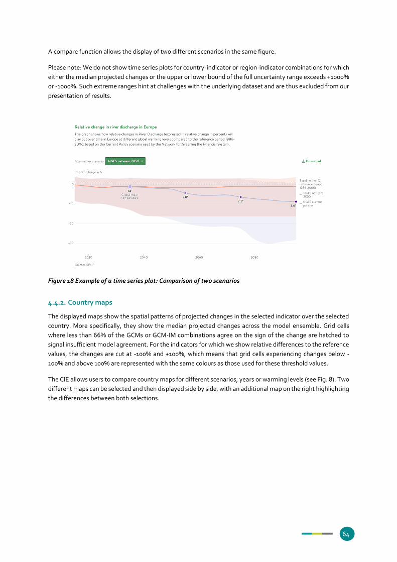
64

A compare function allows the display of two different scenarios in the same figure.

Please note: We do not show time series plots for country-indicator or region-indicator combinations for which

either the median projected changes or the upper or lower bound of the full uncertainty range exceeds +1000%

or -1000%. Such extreme ranges hint at challenges with the underlying dataset and are thus excluded from our

presentation of results.

Figure 18 Example of a time series plot: Comparison of two scenarios

4.4.2. Country maps

The displayed maps show the spatial patterns of projected changes in the selected indicator over the selected

country. More specifically, they show the median projected changes across the model ensemble. Grid cells

where less than 66% of the GCMs or GCM-IM combinations agree on the sign of the change are hatched to

signal insufficient model agreement. For the indicators for which we show relative differences to the reference

values, the changes are cut at -100% and +100%, which means that grid cells experiencing changes below -

100% and above 100% are represented with the same colours as those used for these threshold values.

The CIE allows users to compare country maps for different scenarios, years or warming levels (see Fig. 8). Two

different maps can be selected and then displayed side by side, with an additional map on the right highlighting

the differences between both selections.

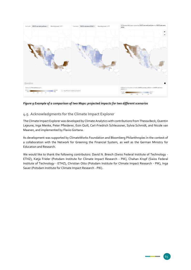
65

Figure 9 Example of a comparison of two Maps: projected impacts for two different scenarios

4.5. Acknowledgments for the Climate Impact Explorer

The Climate Impact Explorer was developed by Climate Analytics with contributions from Thessa Beck, Quentin

Lejeune, Inga Menke, Peter Pfleiderer, Eoin Quill, Carl-Friedrich Schleussner, Sylvia Schmidt, and Nicole van

Maanen, and implemented by Flavio Gortana.

Its development was supported by ClimateWorks Foundation and Bloomberg Philanthropies in the context of

a collaboration with the Network for Greening the Financial System, as well as the German Ministry for

Education and Research.

We would like to thank the following contributors: David N. Bresch (Swiss Federal Institute of Technology -

ETHZ), Katja Frieler (Potsdam Institute for Climate Impact Research - PIK), Chahan Kropf (Swiss Federal

Institute of Technology - ETHZ), Christian Otto (Potsdam Institute for Climate Impact Research - PIK), Inga

Sauer (Potsdam Institute for Climate Impact Research - PIK).

66

Glossary

The following table lists a number of key terms and acronyms used within this document, and gives definitions

and further information. Some of the definitions are taken from the glossaries of the fourth assessment report

and the special report on 1.5 °C of the IPCC (IPCC 2007, 2018b), where much more terms and more extensive

explanations can be found (e.g. https://www.ipcc.ch/sr15/chapter/glossary).

Term Acronym Definition

Agriculture, Forestry and

Other Land Use

AFOLU The Agriculture, Forestry and Other Land Use is a

unique sector since the mitigation potential is derived

from both an enhancement of removals of greenhouse

gases (GHG), as well as reduction of emissions through

management of land and livestock.

Bioenergy Energy derived from any form of biomass or its

metabolic by-products.

Biofuel A fuel, generally in liquid form, produced from

biomass. Biofuels currently include bioethanol from

sugarcane or maize, biodiesel from canola or soybeans,

and black liquor from the paper-manufacturing

process. See also Biomass and Bioenergy.

Biomass Living or recently dead organic material. See also

Bioenergy and Biofuel.

Bioenergy with Carbon

Capture and Storage

BECCS Carbon dioxide capture and storage (CCS) technology

applied to a bioenergy facility. Note that depending on

the total emissions of the BECCS supply chain, carbon

dioxide (CO2) can be removed from the atmosphere.

The integrated assessment models used to develop the

NGFS transition scenarios assume that BECCS

technologies remove carbon dioxide from the

atmosphere. See also Bioenergy and Carbon dioxide

capture and storage (CCS).

Carbon Budget This term refers to three concepts in the literature: (1)

an assessment of carbon cycle sources and sinks on a

global level, through the synthesis of evidence for fossil

fuel and cement emissions, land-use change emissions,

ocean and land CO2 sinks, and the resulting

atmospheric CO2 growth rate. This is referred to as the

global carbon budget; (2) the estimated cumulative

amount of global carbon dioxide emissions that that

is estimated to limit global surface temperature to

a given level above a reference period, taking into

account global surface temperature contributions of

other GHGs and climate forcers; (3) the distribution of

the carbon budget defined under (2) to the regional,

67

national, or sub-national level based on considerations

of equity, costs or efficiency.

Carbon dioxide CO2 A naturally occurring gas, CO2 is also a by-product of

burning fossil fuels (such as oil, gas and coal), of

burning biomass, of land-use changes (LUC) and of

industrial processes (e.g., cement production). It is

the principal anthropogenic greenhouse gas (GHG)

that affects the Earth’s radiative balance. It is the

reference gas against which other GHGs are

measured and therefore has a global warming

potential (GWP) of 1.

Carbon Capture and

Storage

CCS A process in which a relatively pure stream of carbon

dioxide (CO2) from industrial and energy-related

sources is separated (captured), conditioned,

compressed and transported to a storage location

for long-term isolation from the atmosphere.

Sometimes referred to as Carbon capture and storage.

Carbon Dioxide Removal CDR Anthropogenic activities removing CO2 from the

atmosphere and durably storing it in geological,

terrestrial, or ocean reservoirs, or in products. It

includes existing and potential anthropogenic

enhancement of biological or geochemical sinks and

direct air capture and storage, but excludes natural CO2

uptake not directly caused by human activities.

Carbon price (also

emissions price)

The price for avoided or released carbon dioxide (CO2)

or CO2-equivalent emissions. This may refer to the rate

of a carbon tax, or the price of emission permits. In

many models that are used to assess the economic

costs of mitigation, carbon prices are used as a proxy to

represent the level of effort in mitigation policies.

Global Change

Assessment Model

GCAM GCAM is an integrated tool for exploring the dynamics

of the coupled human-Earth system and the response

of this system to global changes.

http://www.globalchange.umd.edu/gcam

Global climate model

(also referred to as

general circulation

model)

GCM A numerical representation of the climate system

based on the physical, chemical and biological

properties of its components, their interactions and

feedback processes, and accounting for some of its

known properties. The climate system can be

represented by models of varying complexity; that is,

for any one component or combination of components

a spectrum or hierarchy of models can be identified,

differing in such aspects as the number of spatial

dimensions, the extent to which physical, chemical or

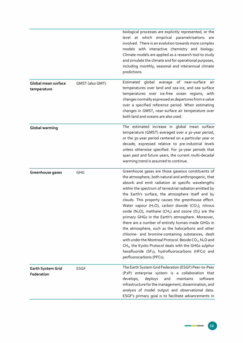
68

biological processes are explicitly represented, or the

level at which empirical parametrisations are

involved. There is an evolution towards more complex

models with interactive chemistry and biology.

Climate models are applied as a research tool to study

and simulate the climate and for operational purposes,

including monthly, seasonal and interannual climate

predictions.

Global mean surface

temperature

GMST (also GMT) Estimated global average of near-surface air

temperatures over land and sea-ice, and sea surface

temperatures over ice-free ocean regions, with

changes normally expressed as departures from a value

over a specified reference period. When estimating

changes in GMST, near-surface air temperature over

both land and oceans are also used.

Global warming The estimated increase in global mean surface

temperature (GMST) averaged over a 30-year period,

or the 30-year period centered on a particular year or

decade, expressed relative to pre-industrial levels

unless otherwise specified. For 30-year periods that

span past and future years, the current multi-decadal

warming trend is assumed to continue.

Greenhouse gases GHG Greenhouse gases are those gaseous constituents of

the atmosphere, both natural and anthropogenic, that

absorb and emit radiation at specific wavelengths

within the spectrum of terrestrial radiation emitted by

the Earth’s surface, the atmosphere itself and by

clouds. This property causes the greenhouse effect.

Water vapour (H2O), carbon dioxide (CO2), nitrous

oxide (N2O), methane (CH4) and ozone (O3) are the

primary GHGs in the Earth’s atmosphere. Moreover,

there are a number of entirely human-made GHGs in

the atmosphere, such as the halocarbons and other

chlorine- and bromine-containing substances, dealt

with under the Montreal Protocol. Beside CO2, N2O and

CH4, the Kyoto Protocol deals with the GHGs sulphur

hexafluoride (SF6), hydrofluorocarbons (HFCs) and

perfluorocarbons (PFCs).

Earth System Grid

Federation

ESGF The Earth System Grid Federation (ESGF) Peer-to-Peer

(P2P) enterprise system is a collaboration that

develops, deploys and maintains software

infrastructure for the management, dissemination, and

analysis of model output and observational data.

ESGF's primary goal is to facilitate advancements in

69

Earth System Science. It is an interagency and

international effort.

https://esgf.llnl.gov

Energy The amount of work or heat delivered. Energy is

classified in a variety of types and becomes useful to

human ends when it flows from one place to another or

is converted from one type into another. Primary

energy (also referred to as energy sources) is the

energy embodied in natural resources (e.g., coal, crude

oil, natural gas, uranium) that has not undergone any

anthropogenic conversion. It is transformed into

secondary energy by cleaning (natural gas), refining

(oil in oil products) or by conversion into electricity or

heat. When the secondary energy is delivered at the

end-use facilities it is called final energy (e.g.,

electricity at the wall outlet), where it becomes usable

energy (e.g., light). Daily, the sun supplies large

quantities of energy as rainfall, winds, radiation, etc.

Some share is stored in biomass or rivers that can be

harvested by men. Some share is directly usable such

as daylight, ventilation or ambient heat. Renewable

energy is obtained from the continuing or repetitive

currents of energy occurring in the natural

environment and includes non-carbon technologies

such as solar energy, hydropower, wind, tide and

waves and geothermal heat, as well as carbon-neutral

technologies such as biomass.

Integrated Assessment

Model

IAM Integrated assessment models (IAMs) integrate

knowledge from two or more domains into a single

framework. They are one of the main tools for

undertaking integrated assessments.

One class of IAM used in respect of climate change

mitigation may include representations of: multiple

sectors of the economy, such as energy, land use and

land-use change; interactions between sectors; the

economy as a whole; associated GHG emissions and

sinks; and reduced representations of the climate

system. This class of model is used to assess linkages

between economic, social and technological

development and the evolution of the climate system.

Another class of IAM additionally includes

representations of the costs associated with climate

change impacts, but includes less detailed

representations of economic systems. These can be

used to assess impacts and mitigation in a cost–benefit

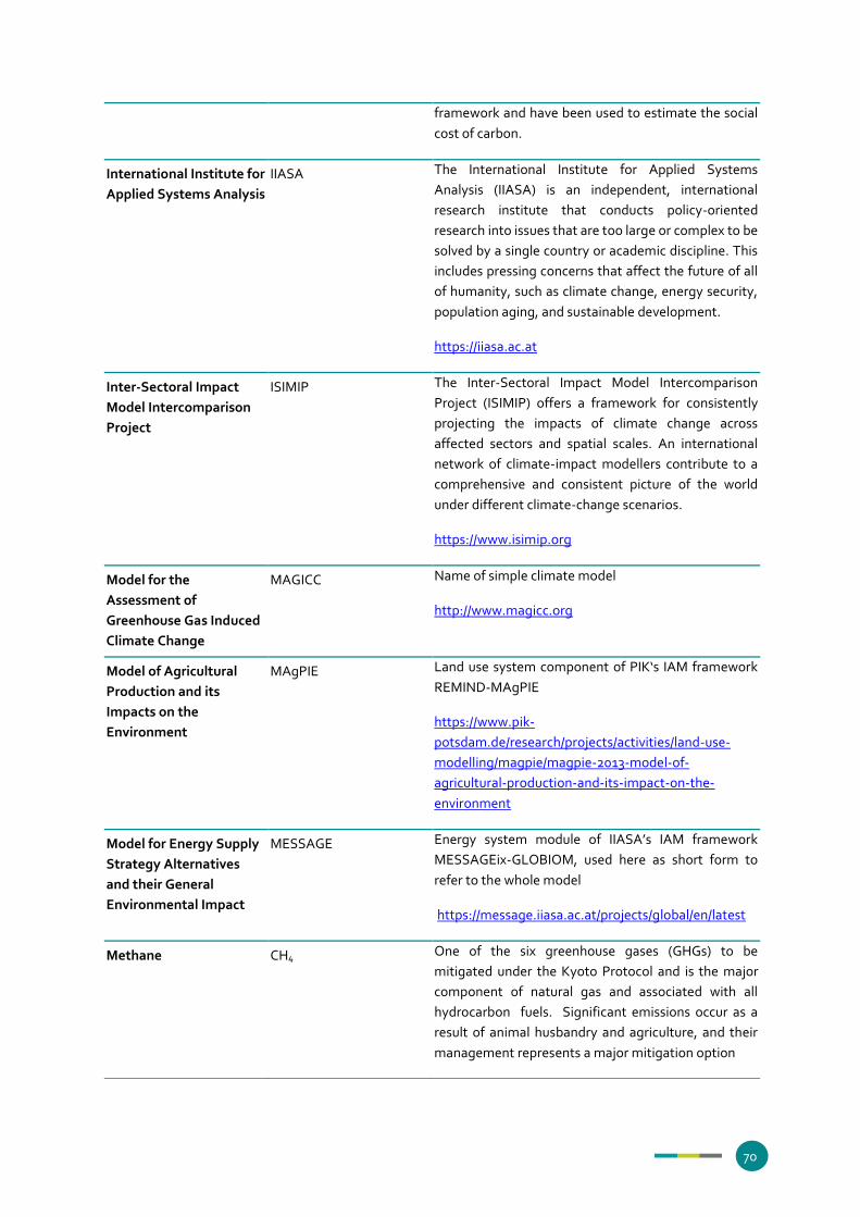
70

framework and have been used to estimate the social

cost of carbon.

International Institute for

Applied Systems Analysis

IIASA The International Institute for Applied Systems

Analysis (IIASA) is an independent, international

research institute that conducts policy-oriented

research into issues that are too large or complex to be

solved by a single country or academic discipline. This

includes pressing concerns that affect the future of all

of humanity, such as climate change, energy security,

population aging, and sustainable development.

https://iiasa.ac.at

Inter-Sectoral Impact

Model Intercomparison

Project

ISIMIP The Inter-Sectoral Impact Model Intercomparison

Project (ISIMIP) offers a framework for consistently

projecting the impacts of climate change across

affected sectors and spatial scales. An international

network of climate-impact modellers contribute to a

comprehensive and consistent picture of the world

under different climate-change scenarios.

https://www.isimip.org

Model for the

Assessment of

Greenhouse Gas Induced

Climate Change

MAGICC Name of simple climate model

http://www.magicc.org

Model of Agricultural

Production and its

Impacts on the

Environment

MAgPIE Land use system component of PIK‘s IAM framework

REMIND-MAgPIE

https://www.pik-

potsdam.de/research/projects/activities/land-use-

modelling/magpie/magpie-2013-model-of-

agricultural-production-and-its-impact-on-the-

environment

Model for Energy Supply

Strategy Alternatives

and their General

Environmental Impact

MESSAGE Energy system module of IIASA’s IAM framework

MESSAGEix-GLOBIOM, used here as short form to

refer to the whole model

https://message.iiasa.ac.at/projects/global/en/latest

Methane CH4 One of the six greenhouse gases (GHGs) to be

mitigated under the Kyoto Protocol and is the major

component of natural gas and associated with all

hydrocarbon fuels. Significant emissions occur as a

result of animal husbandry and agriculture, and their

management represents a major mitigation option

71

Nationally determined

contribution

NDC A term used under the United Nations Framework

Convention on Climate Change (UNFCCC) whereby a

country that has joined the Paris Agreement outlines its

plans for reducing its emissions. Some countries’ NDCs

also address how they will adapt to climate change

impacts, and what support they need from, or will

provide to, other countries to adopt low-carbon

pathways and to build climate resilience.

Net zero CO2 emissions A situation of net zero CO2 emissions is achieved when,

as a result of human activities, the same amount of CO2

is removed from the atmosphere than is emitted into

it. Net CO2 emissions become negative when more CO2

is removed from the atmosphere than emitted into it

(i.e. net negative CO2 emissions).

When multiple greenhouse gases are involved, the

quantification of negative emissions depends on the

climate metric chosen to compare emissions of

different gases (such as global warming potential,

global temperature change potential, and others, as

well as the chosen time horizon).

NGFS Scenario Explorer NGFS SE The NGFS Scenario Explorer is a web-based user

interface for scenario results and historical reference

data and is hosted by IIASA

data.ene.iiasa.ac.at/ngfs.

Nitrous oxide N2O One of the six greenhouse gases (GHGs) to be

mitigated under the Kyoto Protocol. The main

anthropogenic source of N2O is agriculture (soil and

animal manure management), but important

contributions also come from sewage treatment, fossil

fuel combustion, and chemical industrial processes.

N2O is also produced naturally from a wide variety of

biological sources in soil and water, particularly

microbial action in wet tropical forests.

Pathway The term is being used with two slightly different

meanings (see below), including in this report. The

term “Transition pathways” is being used here to refer

to the transition scenarios (to clearer differentiate from

the term “NGFS scenarios”), although one of them

(“Current Policies”) is not a pathway in the strict sense

of meaning (1).

(1) A goal-oriented scenario: The temporal evolution of

natural and/or human systems towards a future goal.

Pathway concepts range from sets of quantitative and

qualitative scenarios or narratives of potential futures

72

to solution-oriented decision-making processes to

achieve desirable societal goals (which means the term

in this meaning is only applicable to a subset of

scenarios, as not all scenarios (e.g. baseline scenarios)

are target-focused). Pathway approaches typically

focus on biophysical, techno-economic, and/or socio-

behavioural trajectories and involve various dynamics,

goals and actors across different scales.

(2) Trajectory of a specific aspect (or variable(s)) in a

scenario, for example the evolution of greenhouse-gas

concentrations in the RCPs. This can lead to confusion,

e.g. when "RCP 8.5" in form of a synecdoche (pars-pro-

toto) is also being used to refer to the underlying

baseline scenario, which is not a pathway in the sense

of meaning (1).

Potsdam Institute for

Climate Impact Research,

Member of the Leibniz

Association

PIK A public research institute in Potsdam, Germany

www.pik-potsdam.de

Pre-industrial The multi-century period prior to the onset of large-

scale industrial activity around 1750. The reference

period 1850–1900 is used to approximate pre-industrial

global mean surface temperature (GMST).

Primary energy

accounting

Several accounting methods are used in energy

analyses that lead to different estimates of primary

energy use.

Three methods are predominantly used: the direct

equivalent method used in UN Statistics and IPCC

reports, the physical energy content method used by the

OECD, the IEA and Eurostat and the substitution

method used by BP and the US EIA.

The direct equivalent method counts one unit of

secondary energy provided from non-combustible

sources as one unit of primary energy, that is, 1 kWh of

electricity or heat is accounted for as 1 kWh = 3.6 MJ of

primary energy.

Regional Model of

Investments and

Development

REMIND Energy system component of PIK‘s IAM framework

REMIND-MAgPIE, used here as short name to refer to

the whole model

https://www.pik-

potsdam.de/research/transformation-

pathways/models/remind

73

Representative

Concentration Pathway

RCP Scenarios that include time series of emissions and

concentrations of the full suite of greenhouse gases

(GHGs) and aerosols and chemically active gases, as

well as land use/land cover (Moss et al., 2010). The

word representative signifies that each RCP provides

only one of many possible scenarios that would lead to

the specific radiative forcing characteristics. The term

pathway emphasises that not only the long-term

concentration levels are of interest, but also the

trajectory taken over time to reach that outcome (Moss

et al., 2010). RCPs usually refer to the portion of the

concentration pathway extending up to 2100, for which

Integrated Assessment Models produced

corresponding emission scenarios.

Shared Socioeconomic

Pathway

SSP Shared Socio-economic Pathways (SSPs) were

developed to complement the RCPs with varying

socio-economic challenges to adaptation and

mitigation (Kriegler et al., 2012; O’Neill et al., 2014).

Based on five narratives, the SSPs describe alternative

socio-economic futures in the absence of climate policy

intervention, comprising sustainable development

(SSP1), regional rivalry (SSP3), inequality (SSP4),

fossil–fueled development (SSP5) and middle-of-the-

road development (SSP2) (O’Neill et al., 2017; Riahi,

Vuuren, et al., 2017). The combination of SSP-based

socio-economic scenarios and Representative

Concentration Pathway (RCP)-based climate

projections provides an integrative frame for climate

impact and policy analysis.

Scenario A plausible description of how the future may develop

based on a coherent and internally consistent set of

assumptions about key driving forces (e.g., rate of

technological change, prices) and relationships. Note

that scenarios are neither predictions nor forecasts, but

are used to provide a view of the implications of

developments and actions.

Sustainable

Development Goals

SDGs The 17 global goals for development for all countries

established by the United Nations through a

participatory process and elaborated in the 2030

Agenda for Sustainable Development, including

ending poverty and hunger; ensuring health and well-

being, education, gender equality, clean water and

energy, and decent work; building and ensuring

resilient and sustainable infrastructure, cities and

consumption; reducing inequalities; protecting land

and water ecosystems; promoting peace, justice and

74

partnerships; and taking urgent action on climate

change.

75

Appendix

Table A1.1 Regional definition of the GCAM model

Model region NGFS SE identifier Iso codes

Africa_Eastern GCAM5.3_NGFS|Africa_Eastern BDI, COM, DJI, ERI, ETH, KEN, MDG, MUS,

REU, RWA, SDN, SOM, UGA

Africa_Northern GCAM5.3_NGFS|Africa_Northern DZA, EGY, ESH, LBY, MAR, TUN

Africa_Southern GCAM5.3_NGFS|Africa_Southern AGO, BWA, LSO, MOZ, MWI, NAM, SWZ,

TZA, ZMB, ZWE

Africa_Western GCAM5.3_NGFS|Africa_Western BEN, BFA, CAF, CIV, CMR, COD, COG, CPV,

GAB, GHA, GIN, GMB, GNB, GNQ, LBR,

MLI, MRT, NER, NGA, SEN, SLE, STP, TCD,

TGO

Argentina GCAM5.3_NGFS|Argentina ARG

Australia_NZ GCAM5.3_NGFS|Australia_NZ AUS, NZL

Brazil GCAM5.3_NGFS|Brazil BRA

Canada GCAM5.3_NGFS|Canada CAN

Central America and

Caribbean

GCAM5.3_NGFS|Central America and

Caribbean

ABW, AIA, ANT, ATG, BHS, BLZ, BMU,

BRB, CRI, CUB, CYM, DMA, DOM, GLP,

GRD, GTM, HND, HTI, JAM, KNA, LCA,

MSR, MTQ, NIC, PAN, SLV, TTO, VCT

Central Asia GCAM5.3_NGFS|Central Asia ARM, AZE, GEO, KAZ, KGZ, MNG, TJK,

TKM, UZB

China GCAM5.3_NGFS|China CHN

Colombia GCAM5.3_NGFS|Colombia COL

EU-12 GCAM5.3_NGFS|EU-12 BGR, CYP, CZE, EST, HUN, LTU, LVA, MLT,

POL, ROM, SVK, SVN

EU-15 GCAM5.3_NGFS|EU-15 AND, AUT, BEL, CHI, DEU, DNK, ESP, FIN,

FLK, FRA, FRO, GBR, GIB, GRC, GRL, IMN,

IRL, ITA, LUX, MCO, NLD, PRT, SHN, SMR,

SPM, SWE, TCA, VAT, VGB, WLF

Europe_Eastern GCAM5.3_NGFS|Europe_Eastern BLR, MDA, UKR

Europe_Non_EU GCAM5.3_NGFS|Europe_Non_EU ALB, BIH, HRV, MKD, MNE, SCG, SRB, TUR,

YUG

European Free

Trade Association

GCAM5.3_NGFS|European Free Trade

Association

CHE, ISL, LIE, NOR, SJM

India GCAM5.3_NGFS|India IND

Indonesia GCAM5.3_NGFS|Indonesia IDN

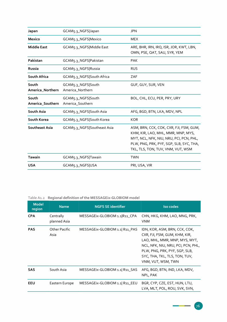
76

Japan GCAM5.3_NGFS|Japan JPN

Mexico GCAM5.3_NGFS|Mexico MEX

Middle East GCAM5.3_NGFS|Middle East ARE, BHR, IRN, IRQ, ISR, JOR, KWT, LBN,

OMN, PSE, QAT, SAU, SYR, YEM

Pakistan GCAM5.3_NGFS|Pakistan PAK

Russia GCAM5.3_NGFS|Russia RUS

South Africa GCAM5.3_NGFS|South Africa ZAF

South

America_Northern

GCAM5.3_NGFS|South

America_Northern

GUF, GUY, SUR, VEN

South

America_Southern

GCAM5.3_NGFS|South

America_Southern

BOL, CHL, ECU, PER, PRY, URY

South Asia GCAM5.3_NGFS|South Asia AFG, BGD, BTN, LKA, MDV, NPL

South Korea GCAM5.3_NGFS|South Korea KOR

Southeast Asia GCAM5.3_NGFS|Southeast Asia ASM, BRN, CCK, COK, CXR, FJI, FSM, GUM,

KHM, KIR, LAO, MHL, MMR, MNP, MYS,

MYT, NCL, NFK, NIU, NRU, PCI, PCN, PHL,

PLW, PNG, PRK, PYF, SGP, SLB, SYC, THA,

TKL, TLS, TON, TUV, VNM, VUT, WSM

Tawain GCAM5.3_NGFS|Tawain TWN

USA GCAM5.3_NGFS|USA PRI, USA, VIR

Table A1.2 Regional definition of the MESSAGEix-GLOBIOM model

Model region

Name NGFS SE identifier Iso codes

CPA Centrally

planned Asia

MESSAGEix-GLOBIOM 1.1|R11_CPA CHN, HKG, KHM, LAO, MNG, PRK,

VNM

PAS Other Pacific

Asia

MESSAGEix-GLOBIOM 1.1| R11_PAS IDN, KOR, ASM, BRN, CCK, COK,

CXR, FJI, FSM, GUM, KHM, KIR,

LAO, MHL, MMR, MNP, MYS, MYT,

NCL, NFK, NIU, NRU, PCI, PCN, PHL,

PLW, PNG, PRK, PYF, SGP, SLB,

SYC, THA, TKL, TLS, TON, TUV,

VNM, VUT, WSM, TWN

SAS South Asia MESSAGEix-GLOBIOM 1.1| R11_SAS AFG, BGD, BTN, IND, LKA, MDV,

NPL, PAK

EEU Eastern Europe MESSAGEix-GLOBIOM 1.1| R11_EEU BGR, CYP, CZE, EST, HUN, LTU,

LVA, MLT, POL, ROU, SVK, SVN,

77

ALB, BIH, HRV, MKD, MNE, SCG,

SRB, TUR, YUG

WEU Western Europe MESSAGEix-GLOBIOM 1.1| R11_WEU AND, AUT, BEL, CHI, DEU, DNK,

ESP, FIN, FLK, FRA, FRO, GBR, GIB,

GRC, GRL, IMN, IRL, ITA, LUX, MCO,

NLD, PRT, SHN, SMR, SPM, SWE,

TCA, VAT, VGB, WLF, CHE, ISL, LIE,

NOR, SJM

FSU Former Soviet

Union

MESSAGEix-GLOBIOM 1.1| R11_FSU ARM, AZE, BLR, GEO, KAZ, KGZ,

MDA, RUS, TJK, TKM, UKR, UZB

LAM Latin America

and the

Caribbean

MESSAGEix-GLOBIOM 1.1| R11_LAM ABW, AIA, ARG, ATG, BHS, BLZ,

BMU, BOL, BRA, BRB, CHL, COL,

CRI, CUB, CYM, DMA, DOM, ECU,

FLK, GLP, GRD, GTM, GUF, GUY,

HND, HTI, JAM, KNA, LCA, MEX,

MSR, MTQ, NIC, PAN, PER, PRY,

SLV, SUR, TCA, TTO, URY, VCT,

VEN, VGB, VIR

MEA Middle-East and

North Africa

MESSAGEix-GLOBIOM 1.1| R11_MEA DZA, EGY, ESH, LBY, MAR, TUN,

ARE, BHR, IRN, IRQ, ISR, JOR, KWT,

LBN, OMN, PSE, QAT, SAU, SYR,

YEM

NAM North America MESSAGEix-GLOBIOM 1.1|

R11_NAM

PRI, USA, VIR, CAN

PAO Pacific OECD MESSAGEix-GLOBIOM 1.1| R11_PAO AUS, NZL, JPN

SSA Sub-Saharan

Africa

MESSAGEix-GLOBIOM 1.1| R11_AFR AGO, BDI, BEN, BFA, BWA, CAF,

CIV, CMR, COD, COG, COM, CPV,

DJI, ERI, ETH, GAB, GHA, GIN, GMB,

GNB, GNQ, KEN, LBR, LSO, MDG,

MLI, MOZ, MRT, MUS, MWI, MYT,

NAM, NER, NGA, REU, RWA, SEN,

SHN, SLE, SOM, STP, SWZ, SYC,

TCD, TGO, TZA, UGA, ZAF, ZMB,

ZWE

78

Table A1.3 Regional definition of the REMIND-MAgPIE model

Model region Name NGFS SE identifier Iso codes

China China, Hong Kong

and Macau

REMIND-MAgPIE 2.1-4.2|CHA CHN, HKG, MAC, TWN

India India REMIND-MAgPIE 2.1-4.2|IND IND

Japan Japan REMIND-MAgPIE 2.1-4.2|JPN JPN

REF Rerforming

economies

REMIND-MAgPIE 2.1-4.2|REF ARM, AZE, BLR, GEO, KAZ, KGZ,

MDA, RUS, TJK, TKM, UKR, UZB

USA United States of

America

REMIND-MAgPIE 2.1-4.2|USA USA

OAS Other Asian

Countries

REMIND-MAgPIE 2.1-4.2|OAS AFG, ASM, BGD, BRN, BTN, CCK,

COK, CXR, FJI, FSM, GUM, IDN,

KHM, KIR, KOR, LAO, LKA, MDV,

MHL, MMR, MNG, MNP, MYS,

NCL, NFK, NIU, NPL, PAK, PCN,

PHL, PLW, PNG, PRK, PYF, SGP,

SLB, THA, TKL, TLS, TON, TUV,

VNM, VUT, WLF, WSM

EUR European Union

(former EU-28 until

31 January 2020)

REMIND-MAgPIE 2.1-4.2|EUR AUT, BEL, BGR, CYP, CZE, DEU,

DNK, ESP, EST, FIN, FRA, FRO,

GBR, GIB, GRC, GRL, HUN, IMN,

IRL, ITA, JEY, LTU, LUX, LVA, MLT,

NLD, POL, PRT, ROU, SVK, SVN,

SWE

LAM Latin America and

the Caribbean

REMIND-MAgPIE 2.1-4.2|LAM ABW, AIA, ARG, ATG, BHS, BLZ,

BMU, BOL, BRA, BRB, CHL, COL,

CRI, CUB, CYM, DMA, DOM, ECU,

FLK, GLP, GRD, GTM, GUF, GUY,

HND, HTI, JAM, KNA, LCA, MEX,

MSR, MTQ, NIC, PAN, PER, PRY,

SLV, SUR, TCA, TTO, URY, VCT,

VEN, VGB, VIR, PRI, VIR

MEA Middle-East, North

Africa and Central

Asia

REMIND-MAgPIE 2.1-4.2|MEA ARE, BHR, DZA, EGY, ESH, IRN,

IRQ, ISR, JOR, KWT, LBN, LBY,

MAR, OMN, PSE, QAT, SAU, SDN,

SYR, TUN, YEM

SSA Sub-Saharan Africa REMIND-MAgPIE 2.1-4.2|SSA AGO, BDI, BWA, COM, DJI, ERI,

ETH, KEN, MDG, MUS, REU, RWA,

SDN, SOM, SSD, UGA, AGO, BWA,

LSO, MOZ, MWI, NAM, SWZ, TZA,

ZMB, ZWE, BEN, BFA, CAF, CIV,

CMR, COD, COG, CPV, GAB, GHA,

GIN, GMB, GNB, GNQ, LBR, MLI,

79

MRT, NER, NGA, SEN, SLE, STP,

TCD, TGO, ZAF

NEU Non-EU Europe REMIND-MAgPIE 2.1-4.2|NEU ALB, AND, BIH, CHE, GGY, HRV,

ISL, LIE, MCO, MKD, MNE, NOR,

NRU, SJM, SMR, SPM, SRB, TUR,

VAT

CAZ Canada, Australia,

New Zealand

REMIND-MAgPIE 2.1-4.2|NEU CAN, AUS, NZL, HMD, SPM

80

Bibliography

Andrijevic, M., Cuaresma, J. C., Muttarak, R., & Schleussner, C. F. (2019) Governance in socioeconomic pathways and its role for future adaptive capacity. Nature Sustainability, 3(1), 35-41.

Aznar-Siguan, G. and Bresch, D. N. (2019)

CLIMADA v1: a global weather and climate risk

assessment platform. Geoscientific Model

Development 12, 3085–3097,

https://doi.org/10.5194/gmd-12-3085-2019

Aznar-Siguan, G., Eberenz, S., Steinmann, C., Vogt, T., Roosli, T., Sauer, I., … Zhu, Q (2021) CLIMADA-project/climada_python_ v2.1.1 (Version v2.1.1.). Zenodo, http://doi.org/10.5281/zenodo.4699962 Bauer, N., Bosetti, V., Hamdi-Cherif, M., Kitous, A., McCollum, D., Méjean, A., Rao, S., Turton, H., Paroussos, L., Ashina, S., Calvin, K., Wada, K., & van Vuuren, D. (2015) CO2 emission mitigation and fossil fuel markets: Dynamic and international aspects of climate policies. Technological Forecasting and Social Change, 90, Part A, 243–256. https://doi.org/10.1016/j.techfore.2013.09.009 Bauer, N., Brecha, R. J., & Luderer, G. (2012) Economics of nuclear power and climate change mitigation policies. Proceedings of the National Academy of Sciences, 109(42), 16805–16810. https://doi.org/10.1073/pnas.1201264109 Bauer, N., Calvin, K., Emmerling, J., Fricko, O., Fujimori, S., Hilaire, J., Eom, J., Krey, V., Kriegler, E., Mouratiadou, I., Sytze de Boer, H., van den Berg, M., Carrara, S., Daioglou, V., Drouet, L., Edmonds, J. E., Gernaat, D., Havlik, P., Johnson, N., … van Vuuren, D. P. (2017) Shared Socio-Economic Pathways of the Energy Sector – Quantifying the Narratives. Global Environmental Change, 42. https://doi.org/10.1016/j.gloenvcha.2016.07.006 Bauer, N., Hilaire, J., Brecha, R. J., Edmonds, J., Jiang, K., Kriegler, E., Rogner, H.-H., & Sferra, F. (2016) Assessing global fossil fuel availability in a scenario framework. Energy, 111, 580–592. https://doi.org/10.1016/j.energy.2016.05.088

Bauer, N., Klein, D., Luderer, G., Hilaire, J., Leimbach, M., Mouratiadou, I., Strefler, J., Pehl, M., Dietrich, J. P., Humpenöder, F., Lotze-Campen, H., Popp, A., Weindl, I., Müller, C., & Kriegler, E. (2014) Climate change stabilization and the energy-land nexus. Paper presented at the International Energy Workshop 2014, Beijng Bauer, N., Rose, S. K., Fujimori, S., Vuuren, D. P. van, Weyant, J., Wise, M., Cui, Y., Daioglou, V., Gidden, M. J., Kato, E., Kitous, A., Leblanc, F., Sands, R., Sano, F., Strefler, J., Tsutsui, J., Bibas, R., Fricko, O., Hasegawa, T., … Muratori, M. (2018) Global energy sector emission reductions and bioenergy use: Overview of the bioenergy demand phase of the EMF-33 model comparison. Climatic Change, 1–16. https://doi.org/10.1007/s10584-018-2226-y Bertram, C., Luderer, G., Pietzcker, R. C., Schmid, E., Kriegler, E., & Edenhofer, O. (2015) Complementing carbon prices with technology policies to keep climate targets within reach. Nature Climate Change, 5(3), 235–239. https://doi.org/10.1038/nclimate2514 Bertram, C., Luderer, G., Popp, A., Minx, J. C., Lamb, F., William, Stevanović, M., Humpenöder, F., Giannousakis, A., & Kriegler, E. (2018) Targeted policies can compensate most of the increased sustainability risks in 1.5 °C mitigation scenarios. Environmental Research Letters, 13(6), 064038. https://doi.org/10.1088/1748-9326/aac3ec Bertram, C., Riahi, K., Hilaire, J., et al. (2021) Energy system developments and investments in the decisive decade for the Paris Agreement goals. Environmental Research Letters. https://doi.org/10.1088/1748-9326/ac09ae Bodirsky, B. L., Popp, A., Weindl, I., Dietrich, J. P., Rolinski, S., Scheiffele, L., Schmitz, C., & Lotze-Campen, H. (2012) N2O emissions from the global agricultural nitrogen cycle – current state and future scenarios. Biogeosciences, 9(10), 4169–4197. https://doi.org/10.5194/bg-9-4169-2012 Bodirsky, Benjamin L., & Popp, A. (2015) Sustainability: Australia at the crossroads. Nature, 527(7576), 40–41. https://doi.org/10.1038/527040a Bondeau, A., Smith, P. C., Zaehle, S., Schaphoff, S., Lucht, W., Cramer, W., Gerten, D., Lotze-Campen, H., Müller, C., Reichstein, M., & Smith, B. (2007) Modelling the role of agriculture for the 20th century global terrestrial carbon balance.

81

Global Change Biology, 13(3), 679–706. https://doi.org/10.1111/j.1365-2486.2006.01305.x Calvin, K., Patel, P., Clarke, L., Asrar, G., Bond-Lamberty, B., Cui, R. Y., Vittorio, A. D., Dorheim, K., Edmonds, J., Hartin, C., Hejazi, M., Horowitz, R., Iyer, G., Kyle, P., Kim, S., Link, R., McJeon, H., Smith, S. J., Snyder, A., … Wise, M. (2019) GCAM v5.1: Representing the linkages between energy, water, land, climate, and economic systems. Geoscientific Model Development, 12(2), 677–698. https://doi.org/10.5194/gmd-12-677-2019 Clarke, J. F., & Edmonds, J. A. (1993) Modelling energy technologies in a competitive market. Energy Economics, 15(2), 123–129. https://doi.org/10.1016/0140-9883(93)90031-L Clarke, L., Jiang, K., Akimoto, K., Babiker, M., Blanford, G., Fisher-Vanden, K., Hourcade, J.-C., Krey, V., Kriegler, E., Löschel, A., McCollum, D., Paltsev, S., Rose, S., Shukla, P. R., Tavoni, M., Zwaan, B. van der, & Vuuren, P. van. (2014) Assessing Transformation Pathways. In O. Edenhofer, R. Pichs-Madruga, Y. Sokona, E. Farahani, S. Kadner, K. Seyboth, A. Adler, I. Baum, S. Brunner, P. Eickemeier, B. Kriemann, J. Savolainen, S. Schlömer, C. von Stechow, T. Zwickel, & J. C. Minx (Eds.), Climate Change 2014: Mitigation of Climate Change. Contribution of Working Group III to the Fifth Assessment Report of the Intergovernmental Panel on Climate Change. Cambridge University Press. http://report.mitigation2014.org/drafts/final-draft-postplenary/ipcc_wg3_ar5_final- draft_postplenary_chapter6.pdf Crespo Cuaresma J. (2017) Income projections for climate change research: A framework based on human capital dynamics, Global Environmental Change, 42, 226-236, ISSN 0959-3780, DOI:10.1016/j.gloenvcha.2015.02.012 Creutzig, F., Agoston, P., Goldschmidt, J. C., Luderer, G., Nemet, G., & Pietzcker, R. C. (2017) The underestimated potential of solar energy to mitigate climate change. Nature Energy, 2, nenergy2017140. https://doi.org/10.1038/nenergy.2017.140 Dasgupta, S.; et al. (forthcoming) Impacts of climate change on combined labour productivity and supply.

Dellink R., Jean Chateau, Elisa Lanzi, Bertrand Magné, (2017) Long-term economic growth projections in the Shared Socioeconomic Pathways, Global Environmental Change, Volume 42, Pages 200-214, ISSN 0959-3780, DOI:10.1016/j.gloenvcha.2015.06.004 Dellink, R., Chateau, J., Lanzi, E., & Magné, B. (2017) Long-term economic growth projections in the Shared Socioeconomic Pathways. Global Environmental Change, 42, 200–214. https://doi.org/10.1016/j.gloenvcha.2015.06.004 Dietrich, J. P., Schmitz, C., Lotze-Campen, H., Popp, A., & Müller, C. (2014) Forecasting technological change in agriculture—An endogenous implementation in a global land use model. Technological Forecasting and Social Change, 81(Supplement C), 236–249. https://doi.org/10.1016/j.techfore.2013.02.003

Eberenz, S. et al. (2021) Regional tropical cyclone

impact functions for globally consistent risk

assessments. Nat. Hazards Earth Syst. Sci., 21, 393–

415, https://doi.org/10.5194/nhess-21-393-2021

Edenhofer, O., Pichs-Madruga, R., & Sokona, Y. (2014) Technical Summary. In Climate Change 2014: Mitigation of Climate Change. Contribution of Working Group III to the Fifth Assessment Report of the Intergovernmental Panel on Climate Change. Cambirdge University Press. Edmonds, J., & Reilly, J. (1983a) Global Energy and CO2 to the Year 2050. The Energy Journal, 4(3), 21–47. Edmonds, J., & Reilly, J. (1983b) Global Energy Production and Use to the Year 2050. Energy, 8(6), 419–432. Edmonds, J., & Reilly, J. (1983c) A long-term global energy- economic model of carbon dioxide release from fossil fuel use. Energy Economics, 5(2), 74–88. https://doi.org/10.1016/0140-9883(83)90014-2 Forster, P., Huppmann, D., Kriegler, E., Mundaca, L., Smith, C., Rogelj, J., & Séférian, R. (2018) Mitigation Pathways Compatible with 1.5°C in the Context of Sustainable Development Supplementary Material. In V. Masson-Delmotte, P. Zhai, H.-O. Pörtner, D. Roberts, J. Skea, & P. R. Shukla (Eds.), Global Warming of 1.5°C. An IPCC Special Report on the impacts of global warming of

82

1.5°C above pre-industrial levels and related global greenhouse gas emission pathways, in the context of strengthening the global response to the threat of climate change, sustainable development, and efforts to eradicate poverty. https://www.ipcc.ch/sr15 Fricko, O., Havlik, P., Rogelj, J., Klimont, Z., Gusti, M., Johnson, N., Kolp, P., Strubegger, M., Valin, H., Amann, M., Ermolieva, T., Forsell, N., Herrero, M., Heyes, C., Kindermann, G., Krey, V., McCollum, D. L., Obersteiner, M., Pachauri, S., … Riahi, K. (2017) The marker quantification of the Shared Socioeconomic Pathway 2: A middle-of-the-road scenario for the 21st century. Global Environmental Change, 42, 251–267. https://doi.org/10.1016/j.gloenvcha.2016.06.004 Frieler, K., Lange, S., Piontek, F., Reyer, C. P. O., Schewe, J., Warszawski, L., Zhao, F., Chini, L., Denvil, S., Emanuel, K., Geiger, T., Halladay, K., Hurtt, G., Mengel, M., Murakami, D., Ostberg, S., Popp, A., Riva, R., Stevanovic, M., … Yamagata, Y. (2017) Assessing the impacts of 1.5 °C global warming – simulation protocol of the Inter-Sectoral Impact Model Intercomparison Project (ISIMIP2b). Geosci. Model Dev., 10(12), 4321–4345. https://doi.org/10.5194/gmd-10-4321-2017

Frieler, K., Lange, S., Piontek, F., Reyer, C. P. O.,

Schewe, J., Warszawski, L., Zhao, F., Chini, L.,

Denvil, S., Emanuel, K., Geiger, T., Halladay, K.,

Hurtt, G., Mengel, M., Murakami, D., Ostberg,

S., Popp, A., Riva, R., Stevanovic, M., …

Yamagata, Y. (2017) Assessing the impacts of

1.5 °C global warming – simulation protocol of the

Inter-Sectoral Impact Model Intercomparison

Project (ISIMIP2b). Geosci. Model Dev., 10(12),

4321–4345. https://doi.org/10.5194/gmd-10-4321-

2017

Fuss, S., Lamb, W. F., Callaghan, M. W., Hilaire, J., Creutzig, F., Amann, T., Tim Beringer, Garcia, W. de O., Hartmann, J., Khanna, T., Luderer, G., Nemet, G. F., Joeri Rogelj, Smith, P., Vicente, J. L. V., Wilcox, J., Dominguez, M. del M. Z., & Minx, J. C. (2018) Negative emissions—Part 2: Costs, potentials and side effects. Environmental Research Letters, 13(6), 063002. https://doi.org/10.1088/1748-9326/aabf9f GEA. (2012) Global Energy Assessment—Toward a Sustainable Future. www.globalenergyassessment.org

Gernaat, D.E.H.J., de Boer, H.S., Daioglou, V. et al. (2021) Climate change impacts on renewable energy supply. Nat. Clim. Chang. https://doi.org/10.1038/s41558-020-00949-9 Gidden M. J., Shinichiro Fujimori , Maarten van den Berg , David Klein,Steven J. Smith, Detlef P. van Vuuren, Keywan Riahi. (2018) A methodology and implementation of automated emissions harmonization for use in Integrated Assessment Models. Environmental Modelling & Software 105 187e200

Gosling S. N., Zaherpour, J. and Ibarreta, D.

(2018) PESETA III: Climate change impacts on

labour productivity, EUR 29423 EN, Publications

Office of the European Union, Luxembourg, 2018,

ISBN 978-92-79- 96912-6, doi:10.2760/07911,

JRC113740.

Grubler, A., Wilson, C., Bento, N., Boza-Kiss, B., Krey, V., McCollum, D. L., Rao, N. D., Riahi, K., Rogelj, J., Stercke, S. D., Cullen, J., Frank, S., Fricko, O., Guo, F., Gidden, M., Havlík, P., Huppmann, D., Kiesewetter, G., Rafaj, P., … Valin, H. (2018) A low energy demand scenario for meeting the 1.5 °C target and sustainable development goals without negative emission technologies. Nature Energy, 3(6), 515–527. https://doi.org/10.1038/s41560-018-0172-6 Harmsen, J. H. M., van Vuuren, D. P., Nayak, D. R., Hof, A. F., Höglund-Isaksson, L., Lucas, P. L., Nielsen, J. B., Smith, P., & Stehfest, E. (2019) Long-term marginal abatement cost curves of non-CO2 greenhouse gases. Environmental Science & Policy, 99, 136–149. https://doi.org/10.1016/j.envsci.2019.05.013

Herger, N., B. M. Sanderson, and Knutti, R.

(2015) Improved pattern scaling approaches for the

use in climate impact studies, Geophys. Res. Lett.,

42, doi:10.1002/2015GL063569.

Hirabayashi, Y., Mahendran, R., Koirala, S. et al.

(2013) Global flood risk under climate change. Nat.

Clim. Change 3, 816–821

https://doi.org/10.1038/nclimate1911

Holland, G. (2008) A Revised Hurricane Pressure–Wind Model. Monthly Weather Review 136, no. 9: 3432–45. https://doi.org/10.1175/2008MWR2395.1

83

Humpenöder, F., Popp, A., Bodirsky, B. L., Weindl, I., Biewald, A., Lotze-Campen, H., Dietrich, J. P., Klein, D., Kreidenweis, U., Müller, C., Rolinski, S., & Stevanovic, M. (2018) Large-scale bioenergy production: How to resolve sustainability trade-offs? Environmental Research Letters, 13(2), 024011. https://doi.org/10.1088/1748-9326/aa9e3b Humpenöder, F., Popp, A., Dietrich, J. P., Klein, D., Lotze-Campen, H., Bonsch, M., Bodirsky, B. L., Weindl, I., Stevanovic, M., & M?ller, C. (2014) Investigating afforestation and bioenergy CCS as climate change mitigation strategies. Environmental Research Letters, 9(6), 064029. https://doi.org/10.1088/1748-9326/9/6/064029 Huppmann, D., Gidden, M., Fricko, O., Kolp, P., Orthofer, C., Pimmer, M., Kushin, N., Vinca, A., Mastrucci, A., Riahi, K., & Krey, V. (2019) The MESSAGEix Integrated Assessment Model and the ix modeling platform (ixmp): An open framework for integrated and cross-cutting analysis of energy, climate, the environment, and sustainable development. Environmental Modelling & Software, 112, 143–156. https://doi.org/10.1016/j.envsoft.2018.11.012 IPCC. (2007) Annex I: Glossary [Verbruggen, A. (ed.)]. In: AR4 Climate Change 2007: Mitigation of Climate Change [Metz B., Davidson O. R., Bosch P. R., Dave R., Meyer L. A. (eds.)]. In Press IPCC. (2013) Technical Summary. In T. F. Stocker, D. Qin, G. Plattner, & Co-Authors (Eds.), Climate Change 2013: The Physical Science Basis. Contribution of Working Group I to the Fifth Assessment Report of the Intergovernmental Panel on Climate Change. Cambridge University Press. IPCC. (2018a) Summary for Policymakers. In Global Warming of 1.5°C. An IPCC Special Report on the impacts of global warming of 1.5°C above pre-industrial levels and related global greenhouse gas emission pathways, in the context of strengthening the global response to the threat of climate change, sustainable development, and efforts to eradicate poverty. IPCC. (2018b) Annex I: Glossary [Matthews, J.B.R. (ed.)]. In: Global Warming of 1.5°C. An IPCC Special Report on the impacts of global warming of 1.5°C above pre-industrial levels and related global greenhouse gas emission pathways, in the context of strengthening the global response to the threat of climate change, sustainable development, and efforts to eradicate poverty [Masson-Delmotte, V.,

P. Zhai, H.-O. Pörtner, D. Roberts, J. Skea, P.R. Shukla, A. Pirani, W. Moufouma-Okia, C. Péan, R. Pidcock, S. Connors, J.B.R. Matthews, Y. Chen, X. Zhou, M.I. Gomis, E. Lonnoy, T. Maycock, M. Tignor, and T. Waterfield (eds.)]. In Press

James, R., Washington, R., Schleussner, C.-F.,

Rogelj, J. and Conway, D. (2017) Characterizing

half-a-degree difference: a review of methods for

identifying regional climate responses to global

warming targets. Wiley Interdiscip. Rev. Clim.

Chang. e457 doi:10.1002/wcc.457

Jewell, J., McCollum, D., Emmerling, J., Bertram, C., Gernaat, D. E. H. J., Krey, V., Paroussos, L., Berger, L., Fragkiadakis, K., Keppo, I., Saadi, N., Tavoni, M., van Vuuren, D., Vinichenko, V., & Riahi, K. (2018) Limited emission reductions from fuel subsidy removal except in energy-exporting regions. Nature, 554(7691), 229–233. https://doi.org/10.1038/nature25467 Jia, G., Shevliakova, E., Artaxo, P., De Noblet-Ducoudré, N., Houghton, R. A., House, J. I., Kitajima, K., Lennard, C., Popp, A., Sirin, A., Sukumar, R., & Verchot, L. (In press) Land–climate interactions. In P. R. Shukla, J. Skea, E. Calvo Buendia, & V. Masson-Delmotte (Eds.), Climate Change and Land: An IPCC special report on climate change, desertification, land degradation, sustainable land management, food security, and greenhouse gas fluxes in terrestrial ecosystems. https://www.ipcc.ch/srccl/ Kalkuhl, M., & Wenz, L. (2020) The Impact of Climate Conditions on Economic Production. Evidence from a Global Panel of Regions. EAERE. http://hdl.handle.net/10419/178288 KC, S., & Lutz, W. (2017) The human core of the shared socioeconomic pathways: Population scenarios by age, sex and level of education for all countries to 2100. Global Environmental Change, 42, 181–192. https://doi.org/10.1016/j.gloenvcha.2014.06.004

Klein Goldewijk, K., Beusen, A., Doelman, J. and

Stehfest, E. (2017) Anthropogenic land use

estimates for the Holocene – HYDE 3.2. Earth Syst.

Sci. Data 9, 927–953, https://doi.org/10.5194/essd-

9-927-2017

84

Klein, D., Goldewijk, K., Beusen, A., van Drecht,

G and de Vos, M (2011) The HYDE 3.1 spatially

explicit database of human-induced global land-

use change over the past 12,000 years. Glob. Ecol.

Biogeogr. 20, 73–86 https://doi.org/10.1111/j.1466-

8238.2010.00587.x

Klein, D., Humpenöder, F., Bauer, N., Dietrich, J. P., Popp, A., Bodirsky, B. L., Bonsch, M., & Lotze-Campen, H. (2014) The global economic long-term potential of modern biomass in a climate-constrained world. Environmental Research Letters, 9(7), 074017. https://doi.org/10.1088/1748-9326/9/7/074017

Knutson, T., Sirutis, J., Zhao, M., Tuleya, R.,

Bender, M., Vecchi, G., Villarini, G, and Chavas,

D. (2015) Global Projections of Intense Tropical

Cyclone Activity for the Late Twenty-First Century

from Dynamical Downscaling of CMIP5/RCP4.5

Scenarios. Journal of Climate. 28.

150729114230005. Doi/10.1175/JCLI-D-15-0129.1.

Koelbl, B. S., Broek, M. A. van den, Faaij, A. P. C., & Vuuren, D. P. van. (2014) Uncertainty in Carbon Capture and Storage (CCS) deployment projections: A cross-model comparison exercise. Climatic Change, 123(3–4), 461–476. https://doi.org/10.1007/s10584-013-1050-7 Kriegler, E., Bertram, C., Kuramochi, T., Jakob, M., Pehl, M., Miodrag Stevanović, Höhne, N., Luderer, G., Minx, J. C., Fekete, H., Hilaire, J., Luna, L., Alexander Popp, Steckel, J. C., Sterl, S., Yalew, A. W., Dietrich, J. P., & Edenhofer, O. (2018) Short term policies to keep the door open for Paris climate goals. Environmental Research Letters, 13(7), 074022. https://doi.org/10.1088/1748-9326/aac4f1 Kriegler, E., O’Neill, B. C., Hallegatte, S., Kram, T., Lempert, R. J., Moss, R. H., & Wilbanks, T. (2012) The need for and use of socio-economic scenarios for climate change analysis: A new approach based on shared socio-economic pathways. Global Environmental Change, 22(4), 807–822. https://doi.org/10.1016/j.gloenvcha.2012.05.005 Kriegler, E., Riahi, K., Bauer, N., Schwanitz, V. J., Petermann, N., Bosetti, V., Marcucci, A., Otto, S., Paroussos, L., Rao, S., Arroyo Currás, T., Ashina, S., Bollen, J., Eom, J., Hamdi-Cherif, M., Longden, T., Kitous, A., Méjean, A., Sano, F., … Edenhofer, O. (2015) Making or breaking

climate targets: The AMPERE study on staged accession scenarios for climate policy. Technological Forecasting and Social Change, 90, Part A, 24–44. https://doi.org/10.1016/j.techfore.2013.09.021 Kriegler, E., Tavoni, M., Aboumahboub, T., Luderer, G., Calvin, K., Demaere, G., Krey, V., Riahi, K., Rösler, H., Schaeffer, M., & Van Vuuren, D. P. (2013) What does the 2°c target imply for a global climate agreement in 2020? The limits study on durban platform scenarios. Climate Change Economics, 04(04), 1340008. https://doi.org/10.1142/S2010007813400083 Kriegler, E., Weyant, J. P., Blanford, G. J., Krey, V., Clarke, L., Edmonds, J., Fawcett, A., Luderer, G., Riahi, K., Richels, R., Rose, S. K., Tavoni, M., & Vuuren, D. P. van. (2014) The role of technology for achieving climate policy objectives: Overview of the EMF 27 study on global technology and climate policy strategies. Climatic Change, 123(3–4), 353–367. https://doi.org/10.1007/s10584-013-0953-7

Lange, S. (2018) Bias correction of surface

downwelling longwave and shortwave radiation for

the EWEMBI dataset, Earth Syst. Dynamics, 9, 627–

645, https://doi.org/10.5194/esd-9-627-2018

Lange, S. (2019) EartH2Observe, WFDEI and ERA-

Interim data Merged and Bias-corrected for ISIMIP

(EWEMBI), https://doi.org/10.5880/pik.2019.004

Lange, S., Volkholz, J., Geiger, T., Zhao, F.,

Vega, I., Veldkamp, T., et al. (2020) Projecting

exposure to extreme climate impact events across

six event categories and three spatial scales. Earth's

Future, 8, e2020EF001616.

https://doi.org/10.1029/2020EF001616

Leimbach M., Elmar Kriegler, Niklas Roming, Jana Schwanitz (2017), Future growth patterns of world regions – A GDP scenario approach, Global Environmental Change, Volume 42, Pages 215-225, ISSN 0959-3780, DOI:10.1016/j.gloenvcha.2015.02.005 Leimbach, M., Bauer, N., Baumstark, L., & Edenhofer, O. (2010) Mitigation Costs in a Globalized World: Climate Policy Analysis with REMIND-R. Environmental Modeling & Assessment, 15(3), 155–173. https://doi.org/10.1007/s10666-009-9204-8

85

Leimbach, M., Bauer, N., Baumstark, L., Luken, M., & Edenhofer, O. (2010) Technological Change and International Trade—Insights from REMIND-R. The Energy Journal, 31(Special Issue), 109–136. https://doi.org/10.5547/ISSN0195-6574-EJ-Vol31-NoSI-5 Leimbach, M., Schultes, A., Baumstark, L., Giannousakis, A., & Luderer, G. (2017) Solution algorithms for regional interactions in large-scale integrated assessment models of climate change. Annals of Operations Research, 255(1–2), 29–45. https://doi.org/10.1007/s10479-016-2340-z Lotze-Campen, H., Müller, C., Bondeau, A., Rost, S., Popp, A., & Lucht, W. (2008) Global food demand, productivity growth, and the scarcity of land and water resources: A spatially explicit mathematical programming approach. Agricultural Economics, 39(3), 325–338. https://doi.org/10.1111/j.1574-0862.2008.00336.x Lotze-Campen, H., Popp, A., Beringer, T., Müller, C., Bondeau, A., Rost, S., & Lucht, W. (2010) Scenarios of global bioenergy production: The trade-offs between agricultural expansion, intensification and trade. Ecological Modelling, 221(18), 2188–2196. https://doi.org/10.1016/j.ecolmodel.2009.10.002 Lucas, P. L., van Vuuren, D. P., Olivier, J. G. J., & den Elzen, M. G. J. (2007) Long-term reduction potential of non-CO2 greenhouse gases. Environmental Science & Policy, 10(2), 85–103. https://doi.org/10.1016/j.envsci.2006.10.007 Luderer, G., Pietzcker, R. C., Bertram, C., Kriegler, E., Meinshausen, M., & Edenhofer, O. (2013) Economic mitigation challenges: How further delay closes the door for achieving climate targets. Environmental Research Letters, 8(3), 034033. https://doi.org/10.1088/1748-9326/8/3/034033 Gidden,M. J., Riahi, K., Smith, S. J., Fujimori, S., Luderer, G., Kriegler, E.,. Van Vuuren, D. P., Van den Berg, M., Feng, L., Klein, D., Calvin, K. et al (2018) Global emissions pathways under different socioeconomic scenarios for use in CMIP6: a dataset of harmonized emissions trajectories through the end of the century” Geosci. Model Dev. Discuss., https://doi.org/10.5194/gmd-2018-266 McCollum, D. L., Zhou, W., Bertram, C., Boer, H.-S. de, Bosetti, V., Busch, S., Després, J., Drouet, L., Emmerling, J., Fay, M., Fricko, O.,

Fujimori, S., Gidden, M., Harmsen, M., Huppmann, D., Iyer, G., Krey, V., Kriegler, E., Nicolas, C., … Riahi, K. (2018) Energy investment needs for fulfilling the Paris Agreement and achieving the Sustainable Development Goals. Nature Energy, 3(7), 589–599. https://doi.org/10.1038/s41560-018-0179-z McFadden, D. (1973) Conditional logit analysis of qualitative choice models. In P. Zarembka (Ed.), Frontiers of Econometrics. Academic Press. McJeon, H., Edmonds, J., Bauer, N., Clarke, L., Fisher, B., Flannery, B. P., Hilaire, J., Krey, V., Marangoni, G., Mi, R., Riahi, K., Rogner, H., & Tavoni, M. (2014) Limited impact on decadal-scale climate change from increased use of natural gas. Nature, 514, 482–485. https://doi.org/10.1038/nature13837 Meinshausen, M., Raper, S. C. B., & Wigley, T. M. L. (2011) Emulating coupled atmosphere-ocean and carbon cycle models with a simpler model, MAGICC6 – Part 1: Model description and calibration. Atmos. Chem. Phys., 11(4), 1417–1456. https://doi.org/10.5194/acp-11-1417-2011

Meinshausen, M., Raper, S. C. B., and Wigley, T.

M. L. (2011) Emulating coupled atmosphere-ocean

and carbon cycle models with a simpler model,

MAGICC6 – Part 1: Model description and

calibration. Atmos. Chem. Phys., 11(4), 1417–1456.

https://doi.org/10.5194/acp-11-1417-2011

Meinshausen, Malte, Meinshausen, N., Hare, W., Raper, S. C. B., Frieler, K., Knutti, R., Frame, D. J., & Allen, M. R. (2009) Greenhouse-gas emission targets for limiting global warming to 2°C. Nature, 458(7242), 1158–1162. https://doi.org/10.1038/nature08017 Moss, R. H., Edmonds, J. A., Hibbard, K. A., Manning, M. R., Rose, S. K., Vuuren, D. P. van, Carter, T. R., Emori, S., Kainuma, M., Kram, T., Meehl, G. A., Mitchell, J. F. B., Nakicenovic, N., Riahi, K., Smith, S. J., Stouffer, R. J., Thomson, A. M., Weyant, J. P., & Wilbanks, T. J. (2010) The next generation of scenarios for climate change research and assessment. Nature, 463(7282), 747–756. https://doi.org/10.1038/nature08823 Mouratiadou, I., Luderer, G., Bauer, N., & Kriegler, E. (2016) Emissions and their drivers: Sensitivity to economic growth and fossil fuel availability across world regions. Climatic Change,

86

136(1), 23–37. https://doi.org/10.1007/s10584-015-1368-4 Müller, C., & Robertson, R. D. (2014) Projecting future crop productivity for global economic modeling. Agricultural Economics, 45(1), 37–50. https://doi.org/10.1111/agec.12088 Nordhaus, W. D. (2017) Revisiting the social cost of carbon. Proceedings of the National Academy of Sciences, 114(7), 1518–1523. https://doi.org/10.1073/pnas.1609244114 Nordhaus, W., & Moffat, A. (2017) A Survey of Global Impacts of Climate Change: Replication, Survey Methods, and a Statistical Analysis. NBER Working Paper Series, 40. https://doi.org/10.3386/w23646 O’Neill, B. C., Kriegler, E., Ebi, K. L., Kemp-Benedict, E., Riahi, K., Rothman, D. S., Ruijven, B. J. van, Vuuren, D. P. van, Birkmann, J., Kok, K., Levy, M., & Solecki, W. (2017) The Roads Ahead: Narratives for Shared Socioeconomic Pathways describing World Futures in the 21st Century. Global Environmental Change, 42, 169–180. https://doi.org/10.1016/j.gloenvcha.2015.01.004 O’Neill, B. C., Kriegler, E., Riahi, K., Ebi, K. L., Hallegatte, S., Carter, T. R., Mathur, R., & Vuuren, D. P. (2014) A new scenario framework for climate change research: The concept of shared socioeconomic pathways. Climatic Change, 122(3), 387–400. https://doi.org/10.1007/s10584-013-0905-2 O’Neill, B. C., Riahi, K., & Keppo, I. (2010) Mitigation implications of midcentury targets that preserve long-term climate policy options. Proceedings of the National Academy of Sciences, 107, 1011–1016. Pietzcker, R. C., Longden, T., Chen, W., Fu, S., Kriegler, E., Kyle, P., & Luderer, G. (2014) Long-term transport energy demand and climate policy: Alternative visions on transport decarbonization in energy-economy models. Energy, 64, 95–108. https://doi.org/10.1016/j.energy.2013.08.059 Pietzcker, R. C., Ueckerdt, F., Carrara, S., de Boer, H. S., Després, J., Fujimori, S., Johnson, N., Kitous, A., Scholz, Y., Sullivan, P., & Luderer, G. (2017) System integration of wind and solar power in integrated assessment models: A cross-model evaluation of new approaches. Energy

Economics, 64, 583–599. https://doi.org/10.1016/j.eneco.2016.11.018 Popp, A., Lotze-Campen, H., Leimbach, M., Knopf, B., Beringer, T., Bauer, N., & Bodirsky, B. (2010) On sustainability of bioenergy production: Integrating co-emissions from agricultural intensification. Biomass and Bioenergy. Popp, Alexander, Calvin, K., Fujimori, S., Havlik, P., Humpenöder, F., Stehfest, E., Bodirsky, B. L., Dietrich, J. P., Doelmann, J. C., Gusti, M., Hasegawa, T., Kyle, P., Obersteiner, M., Tabeau, A., Takahashi, K., Valin, H., Waldhoff, S., Weindl, I., Wise, M., … Vuuren, D. P. van. (2017) Land-use futures in the shared socio-economic pathways. Global Environmental Change, 42, 331–345. https://doi.org/10.1016/j.gloenvcha.2016.10.002 Popp, Alexander, Rose, S. K., Calvin, K., Van Vuuren, D. P., Dietrich, J. P., Wise, M., Stehfest, E., Humpenöder, F., Kyle, P., Van Vliet, J., Bauer, N., Lotze-Campen, H., Klein, D., & Kriegler, E. (2014) Land-use transition for bioenergy and climate stabilization: Model comparison of drivers, impacts and interactions with other land use based mitigation options. Climatic Change, 123(3–4), 495–509. https://doi.org/10.1007/s10584-013-0926-x Rao, S., Klimont, Z., Smith, S. J., Van Dingenen, R., Dentener, F., Bouwman, L., Riahi, K., Amann, M., Bodirsky, B. L., van Vuuren, D. P., Aleluia Reis, L., Calvin, K., Drouet, L., Fricko, O., Fujimori, S., Gernaat, D., Havlik, P., Harmsen, M., Hasegawa, T., … Tavoni, M. (2017) Future air pollution in the Shared Socio-economic Pathways. Global Environmental Change, 42, 346–358. https://doi.org/10.1016/j.gloenvcha.2016.05.012 Riahi, K., Kriegler, E., Johnson, N., Bertram, C., den Elzen, M., Eom, J., Schaeffer, M., Edmonds, J., Isaac, M., Krey, V., Longden, T., Luderer, G., Méjean, A., McCollum, D. L., Mima, S., Turton, H., van Vuuren, D. P., Wada, K., Bosetti, V., … Edenhofer, O. (2015) Locked into Copenhagen pledges—Implications of short-term emission targets for the cost and feasibility of long-term climate goals. Technological Forecasting and Social Change, 90, 8–23. https://doi.org/10.1016/j.techfore.2013.09.016 Riahi, K., van Vuuren, D. P., Kriegler, E., Edmonds, J., O’Neill, B. C., Fujimori, S., Bauer, N., Calvin, K., Dellink, R., Fricko, O., Lutz, W., Popp, A., Cuaresma, J. C., Kc, S., Leimbach, M.,

87

Jiang, L., Kram, T., Rao, S., Emmerling, J., … Tavoni, M. (2017) The Shared Socioeconomic Pathways and their energy, land use, and greenhouse gas emissions implications: An overview. Global Environmental Change, 42, 153–168. https://doi.org/10.1016/j.gloenvcha.2016.05.009 Riahi, K., Vuuren, D. P. van, Kriegler, E., Edmonds, J., O’Neill, B. C., Fujimori, S., Bauer, N., Calvin, K., Dellink, R., Fricko, O., Lutz, W., Popp, A., Cuaresma, J. C., KC, S., & Leimbach, M. (2017) Shared Socioeconomic Pathways: An Overview. Glob. Environ. Change, 42. https://doi.org/10.1016/j.gloenvcha.2016.05.009 Rogelj, J., Huppmann, D., Krey, V., Riahi, K., Clarke, L., Gidden, M., Nicholls, Z., & Meinshausen, M. (2019) A new scenario logic for the Paris Agreement long-term temperature goal. Nature, 573(7774), 357–363. https://doi.org/10.1038/s41586-019-1541-4 Rogelj, J., Meinshausen, M., Sedláček, J., & Knutti, R. (2014) Implications of potentially lower climate sensitivity on climate projections and policy. Environmental Research Letters, 9(3), 031003. https://doi.org/10.1088/1748-9326/9/3/031003 Rogelj, J., Popp, A., Calvin, K. V., Luderer, G., Emmerling, J., Gernaat, D., Fujimori, S., Strefler, J., Hasegawa, T., Marangoni, G., Krey, V., Kriegler, E., Riahi, K., Vuuren, D. P. van, Doelman, J., Drouet, L., Edmonds, J., Fricko, O., Harmsen, M., … Tavoni, M. (2018) Scenarios towards limiting global mean temperature increase below 1.5 °C. Nature Climate Change, 8(4), 325–332. https://doi.org/10.1038/s41558-018-0091-3 Rogelj, J., Shindell, D., Jiang, K., Fifita, S., Forster, P., Ginzburg, V., Handa, C., Kheshgi, H., Kobayashi, S., Kriegler, E., Mundaca, L., Séférian, R., & Vilariño, M. V. (2018) Mitigation pathways compatible with 1.5°C in the context of sustainable development. In Special Report on the impacts of global warming of 1.5 °C. Intergovernmental Panel on Climate Change. http://www.ipcc.ch/report/sr15/ Russo, S., Sillmann, J., & Fischer, E. M. (2015) Top ten European heatwaves since 1950 and their occurrence in the coming decades. Environmental Research Letters, 10(12), 124003. https://doi.org/10.1088/1748-9326/10/12/124003

Samir KC, Wolfgang Lutz, (2017) The human core of the shared socioeconomic pathways: Population scenarios by age, sex and level of education for all countries to 2100, Global Environmental Change, Volume 42, , Pages 181-192, ISSN 0959-3780, DOI:10.1016/j.gloenvcha.2014.06.004

Sauer, I.J., Reese, R., Otto, C. et al. (2021)

Climate signals in river flood damages emerge

under sound regional disaggregation. Nat Commun

12, 2128. https://doi.org/10.1038/s41467-021-

22153-9

Schaphoff, S., von Bloh, W., Rammig, A., Thonicke, K., Biemans, H., Forkel, M., Gerten, D., Heinke, J., Jägermeyr, J., Knauer, J., Langerwisch, F., Lucht, W., Müller, C., Rolinski, S., & Waha, K. (2017) LPJmL4 – a dynamic global vegetation model with managed land: Part I – Model description. Geoscientific Model Development Discussions, 1–59. https://doi.org/10.5194/gmd-2017-145 Schmitz, C., Biewald, A., Lotze-Campen, H., Popp, A., Dietrich, J. P., Bodirsky, B., Krause, M., & Weindl, I. (2012) Trading more food: Implications for land use, greenhouse gas emissions, and the food system. Global Environmental Change, 22(1), 189–209. https://doi.org/10.1016/j.gloenvcha.2011.09.013 Schwanitz, V. J., Piontek, F., Bertram, C., & Luderer, G. (2014) Long-term climate policy implications of phasing out fossil fuel subsidies. Energy Policy, 67, 882–894. https://doi.org/10.1016/j.enpol.2013.12.015

Scussolini, P. et al. (2016) FLOPROS: an evolving

global database of flood protection standards. Nat.

Hazards Earth Syst. Sci.16, 1049–106,

https://doi.org/10.5194/nhess-16-1049-2016

Sferra, F., van Ruijven, B., Riahi, K. (2021)

Downscaling IAMs results to the country level – a

new algorithm. IIASA report (forthcoming)

Strefler, J., Luderer, G., Aboumahboub, T., & Kriegler, E. (2014) Economic impacts of alternative greenhouse gas emission metrics: A model-based assessment. Climatic Change. https://doi.org/10.1007/s10584-014-1188-y Strefler, J., Luderer, G., Kriegler, E., & Meinshausen, M. (2014) Can air pollutant controls

88

change global warming? Environmental Science & Policy, 41, 33–43. https://doi.org/10.1016/j.envsci.2014.04.009 Tavoni, M., Kriegler, E., Aboumahboub, T., Calvin, K., De Maere, G., Wise, M., Klein, D., Jewell, J., Kober, T., Lucas, P., Luderer, G., McCollum, D., Marangoni, G., Riahi, K., & Van Vuuren, D. (2013) The distribution of the major economies’ effort in the durban platform scenarios. Climate Change Economics, 04(04), 1340009. https://doi.org/10.1142/S2010007813400095 TWI2050—The World in 2050. (2018) Transformations to Achieve the Sustainable Development Goals. International Institute for Applied Systems Analysis (IIASA). Available at: http://pure.iiasa.ac.at/15347 UNEP. (2018) The Emissions Gap Report 2018. United Nations Environment Programme (UNEP), Nairobi, Kenya. https://www.unenvironment.org/resources/emissions-gap-report-2018 UNEP-FI. (2018) Extending our Horizons: Assessing Credit Risk and Opportunity in a Changing Climate. United Nations Environment – Finance Initiative. https://www.unepfi.org/news/themes/climate-change/extending-our-horizons/

Van Vuuren, D.P., Edmonds, J., Kainuma, M. et

al. (2011) The representative concentration

pathways: an overview. Climatic Change 109, 5.

https://doi.org/10.1007/s10584-011-0148-z

Velders, G. J. M., Fahey, D. W., Daniel, J. S., Andersen, S. O., & McFarland, M. (2015) Future atmospheric abundances and climate forcings from scenarios of global and regional hydrofluorocarbon (HFC) emissions. Atmospheric Environment, 123, Part A, 200–209. https://doi.org/10.1016/j.atmosenv.2015.10.071 Vicedo-Cabrera, A. M., Guo, Y., Sera, F., Huber, V., Schleussner, C.-F., Mitchell, D., Tong, S., Coelho, M. de S. Z. S., Saldiva, P. H. N., Lavigne, E., Correa, P. M., Ortega, N. V., Kan, H., Osorio, S., Kyselý, J., Urban, A., Jaakkola, J. J. K., Ryti, N. R. I., Pascal, M., … Gasparrini, A. (2018) Temperature-related mortality impacts under and beyond Paris Agreement climate change scenarios. Climatic Change, 150(3), 391–402. https://doi.org/10.1007/s10584-018-2274-3

Weindl, I., Lotze-Campen, H., Popp, A., Müller, C., Havlík, P., Mario Herrero, Schmitz, C., & Rolinski, S. (2015) Livestock in a changing climate: Production system transitions as an adaptation strategy for agriculture. Environmental Research Letters, 10(9), 094021. https://doi.org/10.1088/1748-9326/10/9/094021

Willner, S. N., Levermann, A., Zhao, F. and

Frieler, K. (2018) Adaptation required to preserve

future high-end river flood risk at present levels.

Sci. Adv. 4, eaao1914, DOI: 10.1126/sciadv.aao1914

Willner, S. N., Otto, C. and Levermann, A. (2018)

Global economic response to river floods. Nat.

Clim. Change 8, 594–598,

https://doi.org/10.1038/s41558-018-0173-2