Carbon and water cycling in a Bornean tropical rainforest under current and future climate scenarios

Carbon and water cycling in a Bornean tropical rainforest

under current and future climate scenarios

Tomo�omi Kumagai a,b,*, Gabriel G. Katul b,c, Amilcare Porporato c,Taku M. Saitoh d, Mizue Ohashi e, Tomoaki Ichie f, Masakazu Suzuki g

a University Forest in Miyazaki, Kyushu University, Shiiba-son, Miyazaki 883-0402, Japanb Nicholas School of the Environment and Earth Sciences, Box 90328, Duke University, Durham, NC 27708-0328, USA

c Department of Civil and Environmental Engineering, Box 90287, Duke University, Durham, NC 27708-0287, USAd Research Institute of Kyushu University Forest, Sasaguri, Fukuoka 811-2415, Japan

e Faculty of Forestry, University of Joensuu, Joensuu 80101, Finlandf Center for Tropical Forest Science—Arnold Arboretum, Asia Program, NIE-NTU 637616, Singaporeg Graduate School of Agricultural and Life Sciences, The University of Tokyo, Tokyo 113-8657, Japan

Received 29 April 2004; received in revised form 5 October 2004; accepted 8 October 2004

Abstract

We examined how the projected increase in atmospheric CO2 and concomitant shifts in air temperature and precipitation affect

water and carbon fluxes in an Asian tropical rainforest, using a combination of field measurements, simplified hydrological and car-

bon models, and Global Climate Model (GCM) projections. The model links the canopy photosynthetic flux with transpiration via a

bulk canopy conductance and semi-empirical models of intercellular CO2 concentration, with the transpiration rate determined

from a hydrologic balance model. The primary forcing to the hydrologic model are current and projected rainfall statistics. A main

novelty in this analysis is that the effect of increased air temperature on vapor pressure deficit (D) and the effects of shifts in pre-

cipitation statistics on net radiation are explicitly considered. The model is validated against field measurements conducted in a trop-

ical rainforest in Sarawak, Malaysia under current climate conditions. On the basis of this model and projected shifts in climatic

statistics by GCM, we compute the probability distribution of soil moisture and other hydrologic fluxes. Regardless of projected

and computed shifts in soil moisture, radiation and mean air temperature, transpiration was not appreciably altered. Despite

increases in atmospheric CO2 concentration (Ca) and unchanged transpiration, canopy photosynthesis does not significantly

increase if Ci/Ca is assumed constant independent of D (where Ci is the bulk canopy intercellular CO2 concentration). However,

photosynthesis increased by a factor of 1.5 if Ci/Ca decreased linearly with D as derived from Leuning stomatal conductance for-

mulation [R. Leuning. Plant Cell Environ 1995;18:339–55]. How elevated atmospheric CO2 alters the relationship between Ci/Ca and

D needs to be further investigated under elevated atmospheric CO2 given its consequence on photosynthesis (and concomitant car-

bon sink) projections.

� 2004 Elsevier Ltd. All rights reserved.

Keywords: Elevated CO2; Stochastic processes; Water balance; Tropical rainforest; Photosynthesis; Transpiration

1. Introduction

The projected growth in atmospheric greenhouse

gases within the coming century, as summarized by the

Intergovernmental Panel on Climate Change report

(e.g., [19]), will significantly impact global and regional

0309-1708/$ - see front matter � 2004 Elsevier Ltd. All rights reserved.

doi:10.1016/j.advwatres.2004.10.002

* Corresponding author. Fax: +81 983 38 1004.

E-mail addresses: [email protected] (T. Kumagai),

[email protected] (G.G. Katul), [email protected] (A. Porporato),

[email protected] (T.M. Saitoh), [email protected]

(M. Ohashi), [email protected] (T. Ichie), [email protected]

tokyo.ac.jp (M. Suzuki).

Advances in Water Resources 27 (2004) 1135–1150

www.elsevier.com/locate/advwatres

mailto:[email protected]








temperatures with concomitant modifications to precip-

itation patterns. Tropical rainforests are among the

most important biomes in terms of annual primary pro-

ductivity and water cycling; hence, assessing their sensi-

tivity to potential shifts in global and regional

temperatures and precipitation patterns is a necessary

first step to quantifying future local, regional, and global

carbon and water cycling. Although these forests now

cover only 12% of the total land surface [10], they con-

tain about 40% of the carbon in the terrestrial biosphere

[63] and are responsible for about 50% of terrestrial

gross primary productivity [13]. Also, tropical rainfor-

ests are a major source of global land surface evapora-

tion [5] with profound influences on both global and

regional climate and hydrological cycling (e.g.,

[31,45]). This large latent energy fluxes from tropical

rainforests is known to influence global atmospheric cir-

culation patterns [50].

Although tropical forests in Southeast Asia are about

17% of the total tropical rainforest area [10], relative

deforestation rates [38] and estimated resulting CO2

emissions [20,38] are highest in this region. These forests

remain a viable resource for the economies of several

Southeast Asian countries such as Malaysia, yet their

potential as a carbon sink received much less attention

than those of Amazonian rainforests (e.g., [9,12,14,

17,35,39,40,62,64,65]).

What is also lacking is an understanding of how

hydrologic changes in future climates might impact the

carbon cycling in these tropical rainforests, the subject

of this investigation. Climate of the maritime environ-

ments in Southeast Asian tropics is quite different from

those of environments of South American and Central

African tropics. While there are clearly periodic dry

periods in South American and Central African tropics,

maritime Southeast Asian tropics do not have phase-

locked dry period [29] because this climatic condition

is formed by a combination of a summer monsoon from

the Indian Ocean, a winter monsoon from the Pacific

Ocean and the South China Sea, and Madden and Ju-

lian Oscillation (MJO). As a result, the solar radiation

and the air temperature have small seasonal variations

and the annual rainfall is evenly distributed throughout

the year [22,29]. However, there are some unpredict-

able intra-annual dry spells [28] and inter-annual dry

sequences [27] that may intensify in future climate.

Nomenclature

A daily canopy photosynthetic rate (mol m�2

d�1)

a, b constant physiological parameters describing

the dependence of Ci/Ca on D

Ca ambient CO2 concentration (ppmv)

Ci bulk canopy intercellular CO2 concentration

(ppmv)

D vapor pressure deficit (kPa)

dseason number of days in each season (day)

esatðT0aÞ saturation vapor pressure at T 0

a (kPa)

f limiting factor related to a transpiration pla-

teau at high D

fT(s) probability density function of s

fH(h) probability density function of h

h amount of rainfall when rainfall occurs (mm)

Ic interception (mm d�1)

Ks saturated hydraulic conductivity (mm d�1)

L latent heat of vaporization of water (J kg�1)

P precipitation (mm d�1)

pa atmospheric pressure (kPa)

Pseason total amount of rainfall for each season (mm)

Q leakage loss (mm d�1)

Rag above-ground biomass respiration (lmol m�2

s�1)

RC constant parameter

Reco daytime ecosystem respiration (lmol m�2

s�1)

RH relative humidity (dimensionless)

Rs solar radiation (W m�2)

Rsoil daytime average soil respiration (lmol m�2

s�1)

Rn net radiation (W m�2)

R0n daily average net radiation (W m�2)

s volumetric soil moisture content averaged

over the 0–50 cm soil layer (mm)

t time (day)

T 0a daytime average air temperature (�C)

Tr transpiration (mm d�1)

WUE water use efficiency (lmolCO2 mmol�1H2O)

a Priestley–Taylor coefficient

b constant parameter

c psychrometric constant (Pa K�1)

D rate of change of saturation water vapor pres-

sure with temperature (Pa K�1)

g mean depth of rainfall events (mm)

H relative extractable water in the soil (m3 m�3)

j1, j2, j3 unit conversion factors

1/k mean interval time between rainfall events

(day)

qw density of water (kg m�3)

s interval between rainfall events (day)

1136 T. Kumagai et al. / Advances in Water Resources 27 (2004) 1135–1150

Intra-annual dry spells, in particular, occur every year

and often throughout the year.

Our goal is to investigate how carbon and water cy-

cling of a lowland dipterocarp forest in Southeast

Asian humid tropics will respond to current and pro-

jected atmospheric CO2 concentration and climate

(i.e., air temperature and precipitation patterns). This

work builds on an earlier study that investigated how

the hydrologic budgets are altered by projected shifts

in precipitation only using field measurements, Global

Climate Model (GCM) simulation output, and a sim-

plified hydrologic model [26]. In the present study, we

go further and use these GCM simulation outputs of

current and future air temperature and precipitation

statistics, projected atmospheric CO2 concentration, a

carbon flux model [24] combined with a simplified

hydrological model described in [54,30,52], and field

measurements conducted over a 2-year period to ad-

dress the study goals. Prior to assessing the carbon

and water budget for future climate scenarios, the

model is first validated with field measurements con-

ducted in a tropical rainforest in Lambir Hills National

Park, Sarawak, Malaysia, over a 2-year period, de-

scribed next.

2. Study site and measurements

While much of the site and instrument description

relevant to the hydrologic cycle are presented in [26], a

review and description of the carbon flux measurements

are provided for completeness.

2.1. Site description

The experiment was carried out in a natural forest in

Lambir Hills National Park (4�12 0N, 114�02 0E), 30 km

south of Miri City, Sarawak, Malaysia (Fig. 1). A 4

ha experimental plot at an altitude of 200 m and on a

gentle slope (<5�) was used in this project. An 80-m-tall

canopy crane with a 75-m-length rotating jib was con-

structed in the center of this plot to provide access to

the upper canopy. Observational stage at 59.0 m high

was devoted to eddy-covariance flux measurements.

The canopy height surrounding the crane is about 40

m but the height of emergent treetops can reach up to

50 m.

The mean annual rainfall at Miri Airport (4�19 0N,

113�59 0E), 20 km from the study site, for the period

1968–2001 was around 2740 mm with some seasonal

variation. For example, the mean rainfall for Septem-

ber–October–November (SON) was around 880 mm

and for March–April–May (MAM) was around 520

mm. The mean annual temperature is around 27 �C with

little seasonal variation (e.g., [29]).

The rain forest in this park consists of two types of

native vegetation common to the whole Borneo, i.e.,

mixed dipterocarp forest and tropical heath forest [68].

The former contains various types of dipterocarp trees,

which cover 85% of the total park area. The soils consist

of red–yellow podzonic soils (Malaysian classification)

or ultisols (USDA Soil Texonomy), with a high sand

content (62–72%), an accumulation of nutrient content

at the surface horizon, a low pH (4.0–4.3), and a high

porosity (54–68%) [23,56].

The leaf area index (LAI) was measured in 2002 using

a pair of plant canopy analyzers (LAI-2000, Li-Cor,

Lincoln, NE) every 5 m on a 30 · 30 m2 subplot. The

LAI ranged from 4.8 to 6.8 m2 m�2 with a mean of

6.2 m2 m�2 [28]. The amount of monthly litter-fall was

evenly distributed throughout the year suggesting minor

variations in LAI.

2.2. Micrometeorological and soil moisture measurements

The following instruments were installed at the top of

the crane, 85.8 m from the forest floor: a solar radio-

meter (MS401, EKO, Tokyo, Japan), an infrared

radiometer (Model PIR, Epply, Newport, RI), and a tip-

ping bucket rain gauge (RS102, Ogasawara Keiki,

Tokyo, Japan). At a separate tower located some

100 m south from the crane, the upward short-wave

radiation and long-wave radiation were measured using

a solar radiometer (CM06E, Kipp & Zonen, Delft,

Netherlands) and an infrared radiometer (Model PIR,

Epply, Newport, RI) installed upside down since

December 15, 2001. Samples for radiation were taken

every 5 s and an averaging period of 10 min was used

(CR10X datalogger, Campbell Scientific, Logan, UT).

These measurements were used to compute net radiation

(Rn; W m�2). Maximum and average total daily solar

radiation was 24.5 and 16.7 MJ m�2 d�1, respectively,

and maximum and average total daily net radiation

was 18.2 and 11.5 MJ m�2 d�1, respectively.

At the subplot for the in-canopy microclimate

measurements, we sampled mean air temperature and

humidity at heights of 41.5, 31.5, 21.5, 11.5, 6.5 and 1.5Fig. 1. Location of Lambir Hills National Park, Sarawak, Malaysia.

T. Kumagai et al. / Advances in Water Resources 27 (2004) 1135–1150 1137

m using a series of ventilated sensors with dataloggers

(H0803208 and RS1, Onset, Pocasset, MA) at 10-min

intervals.

Volumetric soil moisture content and matric potential

were measured in a subplot at 10, 20 and 50 cm below

the forest floor using TDR (CS615, Campbell Scientific,

Logan, UT) and tensiometer (DIK3150, Daiki, Tokyo,

Japan) at 10-min intervals (CR23X datalogger, Camp-

bell Scientific, Logan, UT). The relative extractable

water in the soil (H; m3 m�3) and the soil moisture con-

tent over the 0–50 cm soil layer (s; mm) were computed

as described in [26].

2.3. Flux measurements

A three-dimensional sonic anemometer (DA-600,Kai-

jo, Tokyo, Japan) was installed at 60.2 m, i.e., 20 m above

the mean canopy height. Co-located with the sonic ane-

mometer is an open-path CO2/H2O analyzer (LI-7500,

Li-Cor, Lincoln, NE) placed about 30 cm away. Wind

speeds and gas concentration time series were all sampled

at 10Hz.All variances and covariances required for eddy-

covariance flux estimates were computed over a 30-min

averaging interval using the procedure described in [28].

The CO2 concentration profile measurement within

canopy was carried out about 70 m from the crane.

Air samples were drawn at 1.5, 6.5, 11.5, 21.5, 31.5

and 41.5 m above ground level using diaphragm pumps

and an auto solenoid switching system, and the CO2

concentration was measured using a closed-path CO2

infrared gas analyzer (LI-800, Li-Cor, Lincoln, NE).

The CO2 channels were automatically calibrated every-

day using a N2 gas and a 510 ppmv CO2 standard gas

and all raw data were recorded (CR10X datalogger,

Campbell Scientific, Logan, UT).

The soil CO2 efflux was measured manually in 2002

(DOY 134–137, 234–235, 306–308 and 341–343) using

a portable IRGA (LI-6400, Li-Cor, Lincoln, NE) con-

nected to a chamber (6400-09 soil CO2 flux chamber,

Li-Cor, Lincoln, NE) at 25 points every 10 m on the

40 · 40 m2 subplot. The soil CO2 efflux data were aver-

aged over the subplot for each measurement day, and

were regarded as the daytime average values of the soil

respiration rate. As there were small variations in soil

temperature at a depth of 2 cm during the measurement

period (25–28 �C), the dependency of daytime average

soil respiration (Rsoil) on temperature could not be dis-

cerned. Moreover, the relationship between Rsoil and

soil moisture was not significant. Thus, daytime Rsoil

was regarded as a constant 5.73 lmol m�2 s�1, com-

puted by averaging the daytime Rsoil.

To obtain evaporative flux from a wet canopy, a plot

representative of the 4 ha experimental plot was instru-

mented for throughfall and stemflow measurements. De-

tails on throughfall and stemflow measurements are

presented in [41,26].

2.4. Derivation of canopy transpiration and

photosynthetic rate

Canopy transpiration rate can be obtained as above-

canopy H2O flux when the canopy was dry. Net ecosys-

tem CO2 exchange (NEE) was derived as the sum of the

above-canopy CO2 flux, which is obtained using the

eddy covariance system above the canopy, and the with-

in-canopy storage flux, which is determined by quantify-

ing the rate of change of the CO2 concentration of the

air column within the canopy. Maximum and average

daily transpiration rates during the measurement period

were 5.09 and 2.52 mm d�1, respectively, and daytime

average NEE and its maximum value were �7.06 and

�12.74 lmol m�2 s�1, respectively (negative values de-

note net ecosystem CO2 uptake).

Power system failure and exclusion of unreliable

data limited the amount of runs collected from the flux

measurement system. Available data of the above-

canopy CO2/H2O fluxes and the NEE were 41% and

30% of the total possible period between June 15,

2001 and November 15, 2002, respectively. We filled

data gaps and replaced unreliable data (e.g., data

obtained when rainfall occurred) using the light-re-

sponse curve (Saitoh et al., unpublished data) and

according to Kumagai et al. [29]. In addition, we ob-

tained the daytime ecosystem respiration (Reco) from

the intercept of the light-response curve (average

daytime Reco; 8.83 lmol m�2 s�1) and then proceeded

to derive a relationship between the daytime Reco and

H as given by (Saitoh et al., unpublished data): 0.36

mol m�2 d�1 (0 6 H < 0.5) and 0.42 mol m�2 d�1

(0.5 6 H 6 1.0).

At this site no above-ground biomass respiration

(Rag) measurements were collected, and we used a daily

average Rag of 1.9 lmol m�2 s�1 estimated using the

functional model for tropical rainforest woody tissue

respiration [42] and assuming that wood respiration is

nearly equal to leaf respiration [37]. The daytime Reco

expressed as Rsoil + Rag was 7.6 lmol m�2 s�1. Taking

uncertainties in estimating Rag into account, daytime

Reco obtained from the result of eddy-covariance flux

measurement (i.e., the light response curve) and from

Rsoil + Rag is sufficiently close. Hence, we concluded

the Reco from the eddy-covariance flux measurement

is representative of ecosystem-scale values. As a result,

canopy photosynthetic rate can be obtained by

subtracting the daytime Reco from the daytime NEE

(note that negative values denote net ecosystem CO2

uptake).

While precipitation, solar radiation, and air tempera-

ture have small seasonal variations, intra-annual dry

spells have been reported [28]. As the intra-annual dry

spells often occur throughout the year, transpiration

rate is likely to be overly sensitive to the soil moisture

condition.


3. Methodology

We discuss first the carbon and water cycling model,

as well as its parameterization and testing for this exper-

iment, and then proceed to discuss its usage for assessing

shifts in the carbon and water vapor fluxes following

projected increases in atmospheric CO2 concentration

and concomitant shifts in climatic factors such as precip-

itation, air temperature and humidity and net radiation.

For the model testing, climatic factors time series were

measured and used to drive the model calculations; how-

ever, in our model simulations for future climates, only

precipitation statistics and potential increment in atmo-

spheric CO2 concentration and temperature were avail-

able thereby necessitating a stochastic treatment. The

generation of stochastic precipitation and the other cli-

matic factors time series, and the connections to GCM

simulation outputs are also discussed.

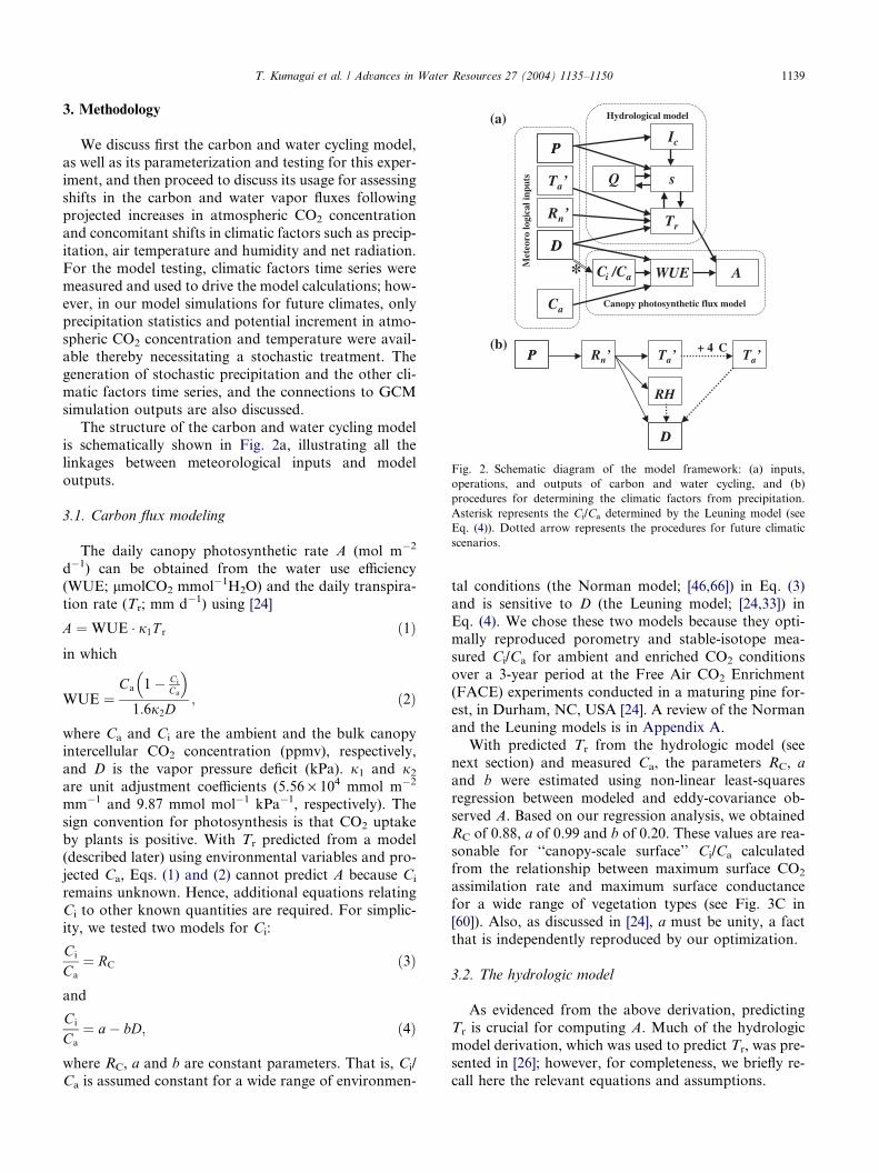
The structure of the carbon and water cycling model

is schematically shown in Fig. 2a, illustrating all the

linkages between meteorological inputs and model

outputs.

3.1. Carbon flux modeling

The daily canopy photosynthetic rate A (mol m�2

d�1) can be obtained from the water use efficiency

(WUE; lmolCO2 mmol�1H2O) and the daily transpira-

tion rate (Tr; mm d�1) using [24]

A ¼ WUE � j1T r ð1Þ

in which

WUE ¼Ca 1� Ci

Ca

� �

1:6j2D; ð2Þ

where Ca and Ci are the ambient and the bulk canopy

intercellular CO2 concentration (ppmv), respectively,

and D is the vapor pressure deficit (kPa). j1 and j2are unit adjustment coefficients (5.56 · 104 mmol m�2

mm�1 and 9.87 mmol mol�1 kPa�1, respectively). The

sign convention for photosynthesis is that CO2 uptake

by plants is positive. With Tr predicted from a model

(described later) using environmental variables and pro-

jected Ca, Eqs. (1) and (2) cannot predict A because Ci

remains unknown. Hence, additional equations relating

Ci to other known quantities are required. For simplic-

ity, we tested two models for Ci:

Ci

Ca

¼ RC ð3Þ

and

Ci

Ca

¼ a� bD; ð4Þ

where RC, a and b are constant parameters. That is, Ci/

Ca is assumed constant for a wide range of environmen-

tal conditions (the Norman model; [46,66]) in Eq. (3)

and is sensitive to D (the Leuning model; [24,33]) in

Eq. (4). We chose these two models because they opti-

mally reproduced porometry and stable-isotope mea-

sured Ci/Ca for ambient and enriched CO2 conditions

over a 3-year period at the Free Air CO2 Enrichment

(FACE) experiments conducted in a maturing pine for-

est, in Durham, NC, USA [24]. A review of the Norman

and the Leuning models is in Appendix A.

With predicted Tr from the hydrologic model (see

next section) and measured Ca, the parameters RC, a

and b were estimated using non-linear least-squares

regression between modeled and eddy-covariance ob-

served A. Based on our regression analysis, we obtained

RC of 0.88, a of 0.99 and b of 0.20. These values are rea-

sonable for ‘‘canopy-scale surface’’ Ci/Ca calculated

from the relationship between maximum surface CO2

assimilation rate and maximum surface conductance

for a wide range of vegetation types (see Fig. 3C in

[60]). Also, as discussed in [24], a must be unity, a fact

that is independently reproduced by our optimization.

3.2. The hydrologic model

As evidenced from the above derivation, predicting

Tr is crucial for computing A. Much of the hydrologic

model derivation, which was used to predict Tr, was pre-

sented in [26]; however, for completeness, we briefly re-

call here the relevant equations and assumptions.

PP Ta’Rn’

RH

Ta’+ 4 C

DD

PP

Ta’

Rn’

DD

Ca

Ci /Ca

Met

eoro

logic

al

inp

uts

WUE

Ic

Tr

sQ

A*

Hydrological model

Canopy photosynthetic flux model

(a)

(b)

Fig. 2. Schematic diagram of the model framework: (a) inputs,

operations, and outputs of carbon and water cycling, and (b)

procedures for determining the climatic factors from precipitation.

Asterisk represents the Ci/Ca determined by the Leuning model (see

Eq. (4)). Dotted arrow represents the procedures for future climatic

scenarios.


For gentle slopes, where lateral movement can be ne-

glected, the vertically integrated continuity equation is

given by

ds

dt¼ P � T r � Ic � Q; ð5Þ

where s is the volumetric soil moisture content averaged

over the root zone (mm), t is the time (day), P is the pre-

cipitation (mm d�1), Tr is, as before, the transpiration

(mm d�1), Ic is the interception (mm d�1) and Q is the

leakage loss (mm d�1) from the soil layer. Given that

the root zone is shallow, we assume that the top 50 cm

soil layer captures much of the root zone water uptake

activity. Also, we assume that Q includes runoff, and

that soil evaporation is insignificant when compared to

the total transpiration flux (given the high LAI at the

site, this assumption is reasonable) (e.g., [25]). The

parameterizations of Tr, Ic, and Q for the site are de-

scribed next.

3.3. Transpiration modeling

The primary forcing variable for transpiration in the

tropics is net available energy. Hence, we use a modified

Priestley and Taylor [53] expression to compute daily

transpiration rate Tr (mmday�1) given by

T r ¼ j3f aD

LqwðDþ cÞR0n; ð6Þ

where a is the Priestley–Taylor coefficient, D is the rate

of change of saturation water vapor pressure with tem-

perature (Pa K�1), L is the latent heat of vaporization of

water (J kg�1), qw is the density of water (1000 kg m�3),

c is the psychrometric constant (66.5 Pa K�1), and R0n is

the daily net radiation above the canopy (W m�2). j3 is

a unit conversion factor (8.64 · 107 mm s m�1 d�1).

Thermodynamic variables D and L are calculated based

on mean air temperature averaged over daylight hours.

Daily net radiation was obtained by averaging hourly

values. In Eq. (6), f is the limiting factor related to a

transpiration plateau at high D (e.g., [43]). Using a func-

tion for stomatal response to increasing D from [48,49],

we assume a simplified form f given by

f ¼1 for D < 1;

1� 0:6 lnD for DP 1:

�

ð7Þ

The model formulation in [48,49] was shown to be

reasonably accurate for a wide range of ecosystem types

and D ranges. A major uncertainty in the transpiration

model is which, for forested ecosystems, is usually less

than its typical 1.26 value because of additional bound-

ary layer, leaf, xylem, and root resistances. We con-

ducted a detailed sensitivity analysis in [26] and

demonstrated that the best estimator of a is

a ¼ 0:49Hþ 0:52 for 0 6 H 6 1:0: ð8Þ

3.4. Interception modeling

In [26], the relationships between daily rainfall P,

throughfall TF and stemflow SF were described as linear

regression equations, and daily interception Ic was re-

lated to P after subtracting both TF and SF from P to

give

Ic ¼

P for 0 6 P < 0:90;

0:13P þ 0:78 for 0:90 6 P < 3:91;

0:084P þ 0:96 for 3:91 6 P :

8

>

<

>

:

ð9Þ

3.5. Leakage losses modeling

In [26], the leakage loss rate (Q) was parameterized

using

Q ¼ KsHb; ð10Þ

where Ks is the saturated hydraulic conductivity (mm

d�1) and b the fitted parameter. The parameters Ks

and b were estimated using non-linear least-squares

regression between s calculated from Eq. (5) and ob-

served s. Based on our regression analysis, we obtained

a Ks of 33.4, typical for loam and sandy loam, and b of

5.3, typical for wet sandy clay loam and dry clay [4]. The

minor differences between Ks and b computed here and

those reported in [26] are strictly due to the differences in

the Tr model.

Details on the ponding and infiltration calculations

are discussed in [26]. When testing the model, measured

time series of the climatic factors (precipitation, radia-

tion, temperature, humidity and CO2) are used to drive

the calculations. However, for future climate simula-

tions, synthetic climatic drivers time series must be con-

structed as described next.

3.6. Simulations of precipitation

Current and future climatic factors time series were

constructed using relationships between precipitation

and other climatic factors obtained in the 2001–2002

observation period, rainfall records collected in 1968–

2001 and GCM outputs for air temperature and precip-

itation for 2070–2100 (details described later). As a

result, current and future time series (i.e., the 1968–

2001 and the 2070–2100) of each hydrological compo-

nent and carbon flow at the site can be computed. From

the simulated time series of each hydrological compo-

nents and carbon flow, their statistics for the period

1968–2001 and 2070 can then be calculated. We then

examine shifts in the statistics of these hydrological com-

ponents and carbon flows based on these anticipated

changes in the climatic (or forcing) factors.

It is necessary to first construct the rainfall time series

because they are needed for constructing other climatic


factors. Current and future rainfall time series (i.e., the

1968–2001 and the 2070–2100) were constructed as the

series of random numbers generated according to prob-

ability distributions representing the 1968–2001 and the

2070–2100 rainfall characteristics at the site. As dis-

cussed in [26], we assumed the frequency and amounts

of rainfall events to be stochastic variables, in which

interval between precipitation events, s (day), is ex-

pressed as a exponential distribution given by

fTðsÞ ¼ k expð�ksÞ for sP 0; ð11Þ

where 1/k is the mean interval time between rainfall

events (day). The amount of rainfall when rainfall oc-

curs, h (mm), is also assumed to be an independent ran-

dom variable, expressed by an exponential probability

density function [30]:

fHðhÞ ¼1

gexp �

1

gh

�

for hP 0; ð12Þ

where g is the mean depth of rainfall events (mm).

For the 1968–2001 rainfall scenario, a long-term data

record obtained at Miri Airport was used to assess the

descriptive skill of the above precipitation model. For

the 2070–2100 rainfall scenarios, a number of transient

climate GCM simulations from the Hadley Centre for

Climate Prediction and Research, available through a

public website, were used. The 2070–2100 time series

of climatic factors at coordinates (2�30 0–5�N, 112�30 0–

116�15 0E) was constructed from the HadCM3 run

(e.g., [11]). The Hadley Centre offers climate change pre-

dictions formulated as differences between current cli-

mate, conventionally defined as 1960–1990, and the

climate at the end of the 21st century, taken to be

2070–2100. As in [26], we used average precipitation

changes in the period 2070–2100 for each of the four

seasons December–February (DJF), March–May

(MAM), June–August (JJA) and September–November

(SON) and obtained average rainfall in periods 1968–

2001 and 2070–2100, respectively, for each season

(Table 1). The Hadley Centre projected precipitation

shifts for this region (i.e., comparing the climate in

1960–1990 with the climate in 2070–2100) are drier

DJF (�180 mm), little change in MAM (�20 mm), wet-ter JJA (�70 mm), and wetter SON (�140 mm). Param-eters 1/k and g in 2070–2100 were obtained, using the

total amount of rainfall Pseason (mm) for each season

using

P season ¼ dseasongk; ð13Þ

where dseason is the number of days in each season (day).

We constructed three types of rainfall scenarios for

2070–2100 (Table 1). Rainfall scenario 2070–2100 A,

which computes 1/k for the 2070–2100 precipitation,

but retains g for 1968–2001. Rainfall scenario 2070–

2100 B, which computes g for 2070–2100, but retains 1/

k as in 1968–2001. That is scenarios 2070–2100 A and

B assume that future changes in rainfall are caused en-

tirely by changes in rainfall frequency or rainfall depth.

In reality, changes in precipitation are due to both fre-

quency and depth. For simulation purposes, it is more

constructive to evaluate these two ‘‘end members’’ as

agents causing precipitation shifts by assigning the entire

shift to be either frequency or depth. To ensure that ‘‘no

surprises’’ exist at some intermediate state, we also con-

structed a rainfall scenario 2070–2100 C as the ‘‘interme-

diate’’ scenario between these two end members, which

computes 1/k and g as mean values between in 1968–

2001 and in 2070–2100 A and B, respectively.

We assumed that a single storm event does not exceed

a day, and that plural storm events during a day can be

Table 1

Rainfall parameters for all scenariosa

DJF MAM JJA SON

2001–2002b Average rainfall (mm/d) 4.92 6.14 6.05 9.73

1/k (day) 1.76 1.98 2.05 1.42

g (mm) 8.7 12.0 12.4 13.8

1968–2001c Average rainfall (mm/d) 8.37 5.85 7.70 9.72

1/k (day) 1.73 2.12 1.82 1.57

g (mm) 14.5 12.0 14.1 15.3

2070–2100d Average rainfall (mm/d) 6.37 5.65 8.45 11.22

Ae 1/k (day) 2.28 2.12 1.67 1.36

Bf g (mm) 10.9 12.1 15.6 17.6

C 1/k (day) 2.00 2.12 1.74 1.47

g (mm) 12.8 12.0 14.7 16.5

a See Eqs. (11) and (12). DJF, December–January–February; MAM, March–April–May; JJA, June–July–August; SON, September–October–

November.b The measurement period September 1, 2001 to August 31, 2002. Average annual rainfall is 2449.5 mm.c Average annual rainfall is 2884.4 mm.d Average annual rainfall is 2888.5 mm.e Values of g are the same as in the 1968–2001 scenario.f Values of 1/k are the same as in the 1968–2001 scenario.


lumped together as a single daily storm. Such a simplify-

ing assumption may be reasonable here because single

storm events exceeding one day seldom occur at least

in the historical record at Miri Airport.

3.7. Current climatic scenario

The current atmospheric CO2 concentration (i.e., the

1968–2001) was assumed to be 360 ppmv. From the

2001–2002 observation results, we obtained relation-

ships between precipitation, P, and the other climatic

factors as follows (see Fig. 2b): (1) In [26], R0n was related

to P via Gaussian random variables with parameters

(mean, l, and standard deviation, r) that vary with P,

that is, 0 6 P < 10 (l = 145.0, r = 33.7), 10 6 P < 20

(l = 108.8, r = 4.8) and 20 6 P (l = 92.3, r = 22.4). (2)

Daytime average air temperature, T 0a (�C), and relative

humidity, RH, were related to R0n through linear regres-

sion models [T 0a ¼ 0:0239R0

n þ 23:48 (R2 = 0.65) and

RH ¼ �0:0015R0n þ 1:0 (R2 = 0.70), respectively]. (3)

An exponential model was fitted to related D to R0n

(D ¼ 0:112 expð0:0118R0nÞ, R2 = 0.75). Using the above

relationships between P and other climatic factors and

the 1968–2001 rainfall scenario, the 1968–2001 climatic

factors time series was constructed.

3.8. Future climatic scenarios

The HadCM3 run assumes that future emissions of

greenhouse gases will follow the IPCC-IS92a scenario

[18], in which the atmospheric concentration of CO2 in-

creases by about 1% per year. According to the IPCC-

IS92a scenario, the atmospheric CO2 concentrations in

2070 and 2100 are 579.2 and 711.7 ppmv, respectively.

Hence, we assumed the 2070–2100 atmospheric CO2

concentration to be 645 ppmv, a mean value between

in 2070 and 2100.

Comparing the climate in 1960–1990 with the climate

in 2070–2100 for this region, the Hadley Centre pro-

jected that surface air temperature increases by 4 �C

for all of the four seasons DJF, MAM, JJA and SON.

The warmer climate experiments using a wide variety

of GCMs suggest that unchanged relative humidity is

realistic [1,21,61,69]. Hence, the modified climate in

2070–2100 might consist of an attendant increase in

atmospheric water vapor concentration but roughly re-

tains its relative humidity as in 1960–1990.

For the 2070–2100 scenarios, we determined the cli-

matic factors, such as R0n, T

0a and D by following proce-

dures (see Fig. 2b): (1) From the 2070–2100 A, B and C

rainfall scenarios, R0n was estimated using the same

method (i.e., the Gaussian random numbers generation)

as when R0n in the 1968–2001 climatic scenario was deter-

mined. (2) From this estimates of R0n, T

0a was initially

estimated using the relationship between T 0a and R0

n de-

rived from the 2001–2002 observations. Also, RH was

estimated using the relationship between RH and R0n

(though the change in RH was minor). (3) In order to

obtain elevated regional air temperature, new estimates

of T 0a were made by adding 4 �C to the initial estimates

of T 0a. (4) From D ¼ esatðT

0aÞð1�RHÞ (where esatðT

0aÞ is

the saturation vapor pressure at T 0a, in kPa), D under

the condition of air temperature increase was computed.

As a result, we obtained the 2070–2100 A, B and C

scenarios as future climatic scenarios. Before discussing

future carbon and water cycling simulations we evaluate

the predictive skills of the simplified carbon and water

cycling model next.

4. Model results

4.1. Model evaluation

Fig. 3 compares calculated cumulative Tr (RTr) and A

(RA) against measurements for June 15, 2001 to Novem-

ber 15, 2002. The model well reproduces measured RTr

and RA despite all the simplifying assumptions. Calcu-

lated RTr at the end of the observation period was only

4% higher than the observed value (Fig. 3a). While cal-

measured

Tr _

mo

del

ed (m

m)

A _measured (mol/m2)

A_

mo

del

ed (m

ol/

m2)

0

0 500 1000

0

100

200

300

400

0 300200 4001001500

500

1000

1500

∑

∑

∑

Tr _ (mm)∑

(a)(b)

Fig. 3. Comparisons between measured and modeled (a) cumulative transpiration rate and (b) cumulative photosynthetic rate (dotted line; the

Norman model, solid line; the Leuning model) for June 15, 2001 to November 15, 2002.


culated RA in the Norman model agreed well with the

observed value (within 3%), the slope of calculated RA

in the Leuning model was not statistically different from

unity (Fig. 3b). This suggests that despite the small dis-

crepancies between observed and calculated values in

the Norman model, the calculation for A under current

climatic conditions is robust to variations in D.

Since the reproduction of s is important because s is

fundamental to estimating A through its effect on a

and Tr, it is necessary to compare how well the measured

and modeled s agree (Fig. 4).

4.2. Carbon and water balances

The model estimated annual Tr and Ic in the measure-

ment period 2001–2002 to be 951.3 and 386.2 mm,

respectively, suggesting that Ic can be up to 40% of Tr

(Table 2). The ratio of Ic to annual precipitation (P)

was 16%. Evapotranspiration, computed as the sum of

Tr and Ic, was 1337.5 mm, accounting for about 55%

of total P. On the other hand, averaged annual Tr and

Ic for the 1968–2001 scenario (hereinafter referred to

as 1968) were 998.6 and 408.5 mm, respectively (Table

2). Note that total P in 2001–2002 was about 440 mm

less than in 1968 scenario. As a result, evapotranspira-

tion and its ratio to total P in 1968 scenario, which is

the ‘‘standard’’ period, were 1407.1 mm and about

49%, respectively. Evapotranspiration studies by Brui-

jinzeel [3] for humid tropical forests suggests that: (1)

annual Tr was, on average, 1045 mm (range 885–1285

mm), (2) Ic was, on average, 13% of incident P (range

between 4.5% and 22%), and (3) annual evapotranspira-

tion ranged from 1310 to 1500 mm. Our values for

evapotranspiration and interception losses for both

2001–2002 and 1968 scenario are comparable to those

reported values. Although the majority of Rn was trans-

formed into latent heat (LE) for both 2001–2002 (78%)

and 1968 scenario (82%), LE positively correlated with

P (Table 2). Interestingly, most measurements on the

fraction of Rn converted to LE = (LE/Rn) reported for

other tropical forests did not consider the evaporation

from the wet canopy. Our results included wet canopy

evaporation in the energy partitioning. When we calcu-

lated LE using only Tr, annual averaged LE/Rn in 2001–

2002 and 1968 scenario were 0.55 and 0.58, respectively.

Our LE/Rn for the dry year (i.e., 2001–2002) and the

standard year (i.e., 1968 scenario) correspond to LE/

Rn measurements collected during the dry and the tran-

sition seasons in the Amazonian tropical forests [40,65],

respectively.

There were little changes in annual P between the sce-

nario 1968 and in the future scenarios 2070–2100A,

2070–2100B and 2070–2100C (hereinafter referred to

as A, B and C, respectively) thereby in annual Ic, while

annual Tr decreased by about 20 mm and annual Q in-

creased by about 30 mm in the future scenarios: some

compensation emerged (Table 2). According to Kuma-

gai et al. [26], seasonal shift in each hydrologic compo-

nent for the future scenarios introduced some

cancellation, that is, on annual timescales, all hydrologic

components experienced minor changes under projected

precipitation scenarios. However, in the future scenarios

of this study, owing to a minor decrease in annual Tr

caused by an increase in D, annual Q mildly increased.

Furthermore, the computed Rn for all the scenarios

were comparable. Hence, the year total LE/Rn for future

scenarios hardly changed (Table 2). Although some dif-

ferences in hydrologic components among the future

scenarios were observed at seasonal timescales, they dis-

s

50

100

150

200

50 100 150 200

_m

od

eled

(m

m)

s _measured (mm)

Fig. 4. Comparison between measured and modeled soil moisture.

Table 2

Annual water and carbon balance for all scenariosa

Scenario P (mm) Tr (mm) Ic (mm) Q (mm) Rn (MJ/m2 d) LEb/Rn A (tC/ha y)

NRc LUc

2001–2002 2449.5 951.3 386.2 1041.4 11.50 0.78 33.3 32.3

1968–2001 2884.4 998.6 408.5 1477.5 11.48 0.82 32.4 33.7

2070–2100A 2891.5 975.9 408.1 1507.5 11.50 0.80 36.4 57.3

2070–2100B 2891.5 978.8 408.9 1504.0 11.49 0.81 36.5 57.5

2070–2100C 2891.5 976.4 406.9 1507.9 11.49 0.80 36.4 57.3

a See Table 1.b Latent heat flux.c NR, the Norman model; LU, the Leuning model.


appeared at annual timescales (see [26]). An immediate

consequence of the computed Tr not significantly chang-

ing in all three future climate scenarios is that all the

changes in photosynthesis are attributed to changes in

WUE, discussed next.

Annual A estimated using the Norman model [46]

and the Leuning model [33] for the measurement period

2001–2002 (33.3 and 32.3 tC ha�1 y�1, respectively) were

not significantly different from those for scenario 1968

(32.4 and 33.7 tC ha�1 y�1, respectively) (Table 2).

Those values are comparable to the 30.4 tC ha�1 y�1 re-

ported for an Amazonian tropical rainforest [37]. An-

nual A in the scenario 1968 calculated using the

Norman and the Leuning models were also comparable

(Table 2). However, when using the Norman model for

the future scenarios a slight increase in annual A was ob-

tained. On the other hand, annual A calculated by the

Leuning model markedly increased for the future sce-

narios (Table 2). For A in the future scenarios computed

by the Norman model, marked increases in D reduced

WUE thereby eliminating the expected enhancement in

WUE attributed to increased Ca. Mathematically, if

RC ( 0.88) is constant,

WUE ¼Cað1� RCÞ

1:6 9:87D

Ca

D

0:12

1:6 9:87:

In the Leuning model, Ci/Ca linearly decreases with

increasing D thereby offsetting the expected reduction

in WUE by increased D. Hence, for the Leuning model,

WUE was primarily affected by an increase in Ca only.

Mathematically, the Leuning model with parameters

a 1 and b = 0.2 leads to a WUE that is independent

of D and is given by

WUE ¼Caf1� ð0:99� 0:2DÞg

1:6 9:87D Ca

0:2

1:6 9:87

which linearly increases with increasing Ca.

Again, on annual timescales, the differences in annual

A among scenarios A, B and C were negligible.

4.3. Soil moisture

Ensemble seasonal probability distributions of soil

moisture content (p(s)) for scenarios 1968, A, B and C

are compared in Fig. 5. p(s) for the measurement period

2001–2002 is also compared. Note that for SON in sce-

nario 1968 and 2001–2002 which have similar rainfall

(see Table 1), p(s) is about the same despite lower s tail

in 2001 caused by preceding drought (Fig. 5d). Depar-

tures in Fig. 5 for the DJF, JJA and whole year p(s)

are primarily due to the frequent droughts in 2001–

2002 (i.e., flatter tails) when compared to ensemble re-

cord of scenario 1968 (see Table 1).

Decrease in heavy rainfall under scenario B does not

affect p(s), while decrease in rainfall frequency increases

the dry mode (Fig. 5a). Under the condition of in-

creased rainfall, some cancellations occur—for exam-

ple, storms with smaller (but more frequent) depths

are likely to be intercepted; however, storms with big-

ger depths (but less frequent) contribute to the drain-

age. Hence, p(s) appears more robust to future shifts

in precipitation when compared to interception or

drainage (see [26]).

4.4. Evapotranspiration

Seasonal cumulative Tr (RTr) and Tr + Ic (R(Tr + Ic))

for the measurement period 2001–2002, current scenario

1968, and future scenarios A, B and C are compared in

Fig. 6.

0

0

0

0

0

80 100 120 140 160 180

(b)

s (mm)

0.01

0.02

0.04

0.03

0.01

0.02

0.03

0.04

0.01

0.02

0.03

0.04

0.01

0.02

0.03

0.04

0.04

0.03

0.02

0.01

p(s

)

(d)

(e)

(c)

(a)

Fig. 5. Modeled probability density functions of soil moisture content

(p(s)) for the measurement period, September 1, 2001 to August 31,

2002 (thick line) and scenarios 1968–2001 (light solid line), the 2070–

2100A (thin solid line), the 2070–2100B (broken line) and the 2070–

2100C (dotted line) (see Table 1). (a) DJF, (b) MAM, (c) JJA, (d) SON

(see Table 1), and whole year.


RTr and R(Tr + Ic) calculated for 2001–2002 were

almost within the range of those calculated using 1968

scenario. However, owing to the frequent droughts in

2001–2002, RTr and R(Tr + Ic) calculated for 2001–

2002 were almost identical to the lower values of RTr

and R(Tr + Ic) for scenario 1968 in DJF and JJA (Fig. 6).

For any future scenario, RTr was not appreciably al-

tered in each of the four seasons (Fig. 6).

Decrease in rainfall amount in DJF reduced Ic under

the future scenarios A, B and C (Fig. 6). For scenario A,

the more frequent light rainfall events were almost per-

fectly intercepted by the canopy, while under scenario B,

the heavier (though less frequent storms) increased Ic(for SON in Fig. 6). For DJF, decreases in Ic determined

decreases in R(Tr + Ic), while for each of the other sea-

sons, R(Tr + Ic) was not appreciably altered.

4.5. Canopy photosynthesis

Figs. 7 and 8 show seasonal cumulative A (RA) for

the measurement period 2001–2002 and scenarios

1968, A, B and C, calculated using the Norman and

the Leuning models, respectively.

While RA calculated by the Leuning model for 2001–

2002 was almost within the range of those for scenario

1968 in any season (Fig. 8), in MAM and JJA there were

large discrepancies between RA calculated by the Nor-

man model for 2001–2002 and for scenario 1968 (Fig.

7). Note that for either model, considering annual RA,

the discrepancies are reduced because parameter Ci/Ca

was determined using yearlong climatic data. Also, on

seasonal timescale, using the Leuning model, the dis-

crepancies between RA in 2001–2002 and in scenario

1968 were minimized because the Ci/Ca can respond to

seasonal variations in D.

For either model, the projected growth in Ca (i.e., 645

ppmv) increased RA for all seasons. However, when

using the Norman model, RA did not increase under fu-

ture scenarios (Fig. 7). The RA calculated by the Leu-

ning model increased up to 170% (Fig. 8). This

suggests that for the Norman model (and constant tran-

spiration), an increase in D roughly cancels the increase

0

20

40

60

80

100

120

140

2001 1968 A B C 2001 1968 A B C 2001 1968 A B C 2001 1968 A B C

SONMAMDJF JJA

A

(mol/

m2)

∑

Fig. 7. Cumulative photosynthetic rate calculated using the Norman model (RC = 0.88) for Ci/Ca in each season for the measurement period,

September 1, 2001 to August 31, 2002 (2001), scenarios 1968–2001 (1968), the 2070–2100A (A), the 2070–2100B (B) and the 2070–2100C (C) (see

Table 1). The top and bottom of the vertical bars in the figure indicate the maximum and minimum, respectively.

0

100

200

300

400

500

2001 1968 A B C 2001 1968 A B C 2001 1968 A B C 2001 1968 A B C

JJA SON MAM DJF

T ,

(T

+ I

c) (

mm

)

∑

∑r

r

Fig. 6. Cumulative transpiration (RTr) and evapotranspiration rate (R(Tr + Ic)) in each season for the measurement period, September 1, 2001 to

August 31, 2002 (2001), scenarios 1968–2001 (1968), the 2070–2100A (A), the 2070–2100B (B) and the 2070–2100C (C) (see Table 1). Blank and

shaded columns represent RTr and cumulative interception (RIc), respectively. The top and bottom of the vertical bars in the figure indicate the

maximum and minimum values, respectively.


in WUE due to increased Ca thereby resulting in a near-

constant RA.

The Ci/Ca estimated using the Norman model under

all scenarios for A estimates was 0.88 (Table 3). How-

ever, using the Leuning model, although the estimated

Ci/Ca in scenario 1968 for A were almost the same as val-

ues estimated using the Norman model (0.87 ± 0.056),

the Ci/Ca in future scenarios A, B and C were signifi-

cantly reduced (0.81 ± 0.059) because of increases in D

(Table 3). As a result, using the Leuning model for fu-

ture scenarios, increases in RA for all season were very

large (Fig. 8).

5. Discussion and conclusions

In a previous study [26], how future shifts in precipi-

tation resulting from an increase in global temperature

affected water reservoirs and fluxes within an Asian

tropical rainforest was examined using a combination

of field measurements, simplified water balance models,

and GCM projections of precipitation. In the present

study, we have examined how the projected increase in

atmospheric CO2 and its concomitant shifts in air tem-

perature, added to shifts in precipitation affect both

water fluxes and photosynthesis within an Asian tropical

rainforest. We used carbon flux model combined with a

simplified hydrological model already developed and

tested for this region and GCM projections of air tem-

perature to address the study objective. The field mea-

surements permitted us to derive key relationships for

present-day climate that tie the ‘‘forcing’’ term with

parameters or state variables. For example, the field

data were used to derive relationships between precipita-

tion and variability in net radiation, air temperature and

air humidity, between transpiration and extractable

water content, between precipitation and interception,

the drainage flow parameters, and the parameters for

describing Ci/Ca.

The Hadley Centre projected precipitation shifts for

this region in 2070–2100 are drier DJF, little change in

MAM, wetter JJA, and wetter SON compared to the cli-

mate in 1968–2001. We assumed that this shift occurs in

one of the two ways: change in precipitation depth or

change in precipitation frequency. In reality, both fre-

quency and depth are likely to change; thus, by explor-

ing the ‘‘end members’’ and an ‘‘intermediate’’

precipitation shift scenarios, we can quantify the ex-

pected changes in hydrologic fluxes and reservoirs.

Based on climate models relative humidity appears

invariant to changes in greenhouse warming (e.g.,

[1,21,61,69]). This invariance in relative humidity, when

combined with a 4 �C temperature increase leads to a

concomitant increase in water vapor pressure deficit that

affects both water use efficiency, and, to a lesser extend

transpiration for the site.

The probability distribution of soil moisture (p(s)) is

sensitive to a decrease in precipitation, in part because

smaller depth (but more frequent) precipitation events

are efficiently intercepted by the ecosystem. On the other

hand, p(s) is robust to an increase in precipitation be-

cause larger depth (but less frequent) precipitation

events increase primarily the drainage. Regardless of

shifts in precipitation (and hence shifts in soil moisture),

radiation and mean air temperature, transpiration is not

appreciably altered. This lack of sensitivity of transpira-

tion to increases in vapor pressure deficit (D) is due to

Table 3

Ci/Ca for the Norman and the Leuning models, for scenarios 1968–

2001, 2070–2100A, 2070–2100B and 2070–2100C

NRa LUa

1968b, Ac, B

and C

1968 A B C

0.88 0.87 (0.056) 0.81 (0.059) 0.81 (0.059) 0.81 (0.059)

Standard deviations are shown in parentheses.a NR, the Norman model; LU, the Leuning model.b 1968, 1968–2001 scenario.c A, 2070–2100A scenario; B, 2070–2100B scenario; C, 2070–2100C

scenario.

0

20

40

60

80

100

120

140

A(m

ol/

m2)

2001 1968 A B C 2001 1968 A B C 2001 1968 A B C 2001 1968 A B C

JJA SONMAMDJF

∑

Fig. 8. Same as Fig. 7 but using the Leuning model for Ci/Ca.


the fact that only a D exceeding 1 kPa will reduce stoma-

tal conductance. Despite increases in atmospheric CO2

concentration and unchanged transpiration, the results

for canopy photosynthesis strongly depend on how Ci/

Ca will respond to D. In the case of a constant Ci/Ca

or even a Ci/Ca that varies with relative humidity

(RH) [24] as is the case with the widely used Ball–Berry

formulation [6], given by

Ci

Ca

1�1

mRHð14Þ

(where m is the Ball–Berry slope parameter), much of

the water use efficiency (WUE) enhancement due to ele-

vated atmospheric CO2 will be counteracted by the in-

crease in D. The latter increase is attributed to a

constant RH and a 4 �C warmer climate. On the other

hand, if Ci/Ca linearly varies with D, as is the case for

the Leuning model, WUE becomes independent of D

and any increase in atmospheric CO2 results in a pro-

portional increase in WUE and photosynthesis if tran-

spiration is unaltered.

In general, under elevated CO2, CO2 uptake of forest

canopies is expected to increase as demonstrated by the

FACE experiment in a Southeastern United States pine

forest (Duke Forest) (e.g., [47,58]). In the Duke Forest

FACE experiment with ambient +200 ppm CO2, the

simpler model (i.e., the Norman model) was sufficient

for reproducing the photosynthesis rate enhancement

through modeling appropriate Ci/Ca [24]. Katul et al.

[24] suggested that the CO2 concentration enhancement

is 1.55 and the computed enhancement in photosynthe-

sis from the Norman model is also 1.55. This estimate is

in agreement with leaf-level measurements of photosyn-

thesis enhancement by Ellsworth (1.56; [7]). It is impor-

tant to note that FACE experiments are generally

designed to maintain similar microclimatic conditions

for ambient and CO2 enriched conditions; hence, differ-

ences between D (or RH) for ambient and enriched plots

is minimum. Schafer et al. [59] showed that for this

Duke Forest FACE experiment, D for ambient and en-

riched plots was similar (see e.g., their Fig. 2). In this

study, however, our values of CO2 uptake estimated

using the Norman model under current +300 ppm

CO2 were not much altered when compared to the ambi-

ent state mainly because of the ratio of Ca/D was not al-

tered. Furthermore, our values of CO2 uptake calculated

using the Norman and the Leuning models were consid-

erably different, because the Leuning model takes the ef-

fect of D into consideration, while the Norman model

does not. It is interesting to note that no FACE experi-

ments currently exist that take into consideration in-

crease in D caused by an increase in air temperature

attendant on the projected growth in CO2.

An important consequence of a change in D but con-

stant RH in a future climate scenario is that if the Ball–

Berry model [6] was used for computing Ci/Ca, future

photosynthesis rate would be similar to those calculated

using the Norman model and would not be appreciably

altered from their present value. For the Leuning model,

photosynthesis increased by a factor of 1.5 when com-

paring current and future climate. Although the Leu-

ning model is generally regarded as a Ball–Berry type

model, this study highlights a fundamental difference be-

tween the two approaches. From a physiological point

of view, stomata respond to D not RH [49].

Although warmer temperatures could increase rates

of all chemical and biochemical processes in plants

and soils up to a point where enzymes disintegrate

(e.g., [57]), the uncertainty over the interaction between

elevated CO2 and temperature (e.g., [16]) is not small. In

general, under elevated CO2, enhancements of photo-

synthetic rate are observed (e.g., [7]). However, in a

few instances, increasing atmospheric CO2 has been

shown to cause down-regulation of photosynthetic rate

(e.g., [15,55]). Preliminary evidence from a FACE exper-

iment in a Southeastern United States hardwood forest

suggests that increasing atmospheric CO2 reduces tran-

spiration rate (e.g., [67]) through a reduction in stomatal

conductance (e.g., [36]). Furthermore, increase in atmo-

spheric CO2 can increase interception by increasing LAI

(e.g., [34]).

On much longer time scales, increases in atmo-

spheric CO2 can induce higher soil water holding capac-

ity because of an increase in soil organic matter content

resulting from increased litter production (e.g., [44,59]).

In the Duke Forest FACE experiment, however, it is

suggested that LAI, stomatal conductance, Ci/Ca and

bulk canopy conductance are, to a first order, unaltered

by elevated CO2 [8,24,51,59]. Thus, the effects of ele-

vated CO2, including its attendant shifts in the other cli-

matic factors, on numerous factors in forest ecosystems

still remain uncertain. Further research is now required

on the effects of elevated CO2 on Southeast Asian rain-

forest ecosystems using extensive and technically diffi-

cult experiments.

Acknowledgments

We thank Hua Seng Lee and Lucy Chong for provid-

ing the opportunity for this study. This work has been

supported by CREST (Core Research for Evolutional

Science and Technology) of JST (Japan Science and

Technology Agency) and a grant from the Ministry of

Education, Science and Culture of Japan (#13760120).

We thank Tohru Nakashizuka for his support and the

many colleagues who helped us with this work. Tomo�o-

mi Kumagai and Gabriel Katul would like to thank

Ram Oren for his useful critique. Gabriel Katul

acknowledges support from Duke University�s Center

on Global Change, the National Science Foundation

(NSF-EAR and NSF-DMS), and the Department of


Energy through their Biological and Environmental Re-

search (BER) Program, the Southeast Regional Center

(SERC) of the National Institute for Global Environ-

mental Change (NIGEC), and the DOE Terrestrial Car-

bon Processes Program (TCP) and the FACE project.

Amilcare Porporato was supported by the DOE-NI-

GEC (Great Plains Regional Center) grant DE-FC02-

03ER63613.

Appendix A. The Norman and the Leuning models for

stomatal conductance

The photosynthetic rate A can be described as

A ¼ gcðCa � CiÞ ¼ gcCa 1�Ci

Ca

�

; ðA:1Þ

where gc is the stomatal conductance, and Ca and Ci are

the ambient and the intercellular CO2 concentration,

respectively.

Wong et al. [66] have shown that the Ci can be

approximated by Ci = 0.80Ca for C3 plants, for a wide

range of environmental conditions, but that this rela-

tionship varies from species to species. According to

Wong et al. [66], Norman [46] assumed that A resulted

from changes in which attempt to hold Ci/Ca constant

(= RC) for a wide range of environmental conditions

(see Eq. (3)).

One widely used gc model is the Ball–Berry model

(see [6]), given by

gc ¼ mARH

CS

þ g0; ðA:2Þ

where m and g0 are empirical parameters, and RH and

CS are relative humidity and CO2 concentration at the

leaf surface, respectively. Eq. (A.2) is an empirical rela-

tionship that incorporates the often-observed correla-

tion between A and gc, and includes the effects of RH

and CS on gc. Using Eqs. (A.1) and (A.2) and upon

neglecting the leaf boundary layer resistance relative to

g�1c (i.e., Ca CS), a closure model for Ci/Ca, given by

Eq. (14), can be derived if g0 is neglected [24].

However, it is widely accepted that stomata respond

to humidity deficit, D, rather than to surface RH (e.g.,

[2]). Furthermore, since A approaches zero when CS ap-

proaches the CO2 compensation point, and Eq. (A.2)

cannot describe stomatal behavior at low CO2 concen-

tration [32]. Leuning [32,33] accounted for those obser-

vations by replacing RH and CS in Eq. (A.2) with a

vapor pressure deficit correction function f (D) and

CS � C respectively, i.e.,

gc ¼ mAf ðDÞ

CS � Cþ g0; f ðDÞ ¼ 1þ

D

D0

� �1

; ðA:3Þ

where D0 is the empirical parameter. Using the same ap-

proach for deriving a closure model for Ci/Ca described

by Eq. (14), the Leuning [33] model reduces to

Ci

Ca

¼1�1

m1�

C

Ca

�

1þD

D0

�

; ðA:4Þ

¼ 1�1

m1�

C

Ca

� �

�1

mD0

1�C

Ca

� �

D: ðA:5Þ

Note that Eq. (A.5) is synonymous with Eq. (4).

References

[1] Allan RP, Ringer MA, Slingo A. Evaluation of moisture in the

Hadley Centre climate model using simulations of HIRS water-

vapour channel radiances. Quart J R Meteorol Soc 2003;129:

3371–89.

[2] Aphalo PJ, Jarvis PG. Do stomata respond to relative humidity?

Plant Cell Environ 1991;14:127–32.

[3] Bruijnzeel LA. Hydrology of moist tropical forests and effects of

conversion: a state of knowledge review. UNESCO: International

Hydrological Programme; 1990.

[4] Campbell GS, Norman JM. An introduction to environmental

biophysics. 2nd ed.. New York: Springer-Verlag; 1998.

[5] Choudhury B, DiGirolamo NE, Susskind J, Darnell WL, Gupta

SK, Asrar G. A biophysical process-based estimate of global land

surface evaporation using satellite and ancillary data, II. Regional

and global patterns of seasonal and annual variations. J Hydrol

1998;205:186–204.

[6] Collatz GJ, Ball JT, Grivet C, Berry JA. Regulation of stomatal

conductance and transpiration: a physiological model of canopy

processes. Agric For Meteorol 1991;54:107–36.

[7] Ellsworth DS. CO2 enrichment in a maturing pine forest: are CO2

exchange and water status in the canopy affected? Plant Cell

Environ 1999;22:461–72.

[8] Ellsworth DS, Oren R, Huang C, Phillips N, Hendrey GR. Leaf

and canopy responses to elevated CO2 in a under free-air CO2

enrichment. Oecologia 1995;104:139–46.

[9] Fan SM, Wofsy SC, Bakwin PS, Jacob DJ. Atmosphere–

biosphere exchange of CO2 and O3 in the central Amazon forest.

J Geophys Res 1990;95(D10):16851–64.

[10] Food and Agriculture Organization. Forest Resources Assessment

1990—Tropical Countries. Rome: FAO Forestry Paper 112; 1993.

[11] Gordon C, Cooper C, Senior CA, Banks H, Gregory JM, Johns

TC, et al. The simulation of SST, sea ice extents and ocean heat

transports in a version of the Hadley Centre coupled model

without flux adjustments. Climate Dynam 2000;16:147–68.

[12] Grace J, Lloyd J, McIntyre J, Miranda A, Meir P, Miranda H,

et al. Fluxes of carbon dioxide and water vapour over an

undisturbed tropical forest in south-west Amazonia. Glob Change

Biol 1995;1:1–12.

[13] Grace J, Malhi Y, Higuchi N, Meir P. Productivity of tropical

forests. In: Roy J, Saugier B, Mooney HA, editors. Terrestrial

global productivity. San Diego: Academic Press; 2001. p. 401–26.

[14] Grace J, Malhi Y, Lloyd J, McIntyre J, Miranda AC, Meir P,

et al. The use of eddy covariance to infer the net carbon dioxide

uptake of Brazilian rain forest. Glob Change Biol 1996;2:209–17.

[15] Griffin KL, Tissue DT, Turnbull MH, Whitehead D. The onset of

photosynthetic acclimation to elevated CO2 partial pressure in

field-growth Pinus radiata D.Don after 4 years. Plant Cell Environ

2001;23:1089–98.

[16] Hikosaka K, Murakami A, Hirose T. Balancing carboxylation

and regeneration of ribulose-1,5-bis-phosphate in leaf photosyn-


thesis: temperature acclimation of an evergreen tree, Quercus

myrsinaefolia. Plant Cell Environ 1999;22:841–9.

[17] Hodnett MG, da Silva LP, da Rocha HR, Senna RC. Seasonal

soil water storage changes beneath central Amazonian rainforest

and pasture. J Hydrol 1995;170:233–54.

[18] Houghton JT, Callander BA, Varney SK, editors. Climate change

1992: The supplementary report to the IPCC scientific assess-

ment. Cambridge: Cambridge University Press; 1992.

[19] Houghton JT, Ding Y, Griggs DJ, Noguer M, van der Linden PJ,

Xiaosu D, editors. Climate change 2001: The scientific

basis. Cambridge: Cambridge University Press; 2001.

[20] Houghton RA, Hackler JL. Emissions of carbon from forestry

and land-use change in tropical Asia. Glob Change Biol

1999;5:481–92.

[21] IngramWJ. On the robustness of the water vapor feedback: GCM

vertical resolution and formulation. J Climate 2002;15:917–21.

[22] Inoue T, Nakamura K, Salamah S, Abbas I. Population dynamics

of animals in unpredictably-changing tropical environments. J

Biosci 1993;18:425–55.

[23] Ishizuka S, Tanaka S, Sakurai K, Hirai H, Hirotani H, Ogino K,

et al. Characterization and distribution of soils at Lambir Hills

National Park in Sarawak, Malaysia, with special reference to soil

hardness and soil texture. Tropics 1998;8:31–44.

[24] Katul GG, Ellsworth DS, Lai C-T. Modelling assimilation and

intercellular CO2 from measured conductance: a synthesis of

approaches. Plant Cell Environ 2000;23:1313–28.

[25] Kelliher FM, Luening R, Raupach MR, Schulze E-D. Maximum

conductances for evaporation from global vegetation types. Agric

For Meteorol 1995;73:1–16.

[26] Kumagai T, Katul GG, Saitoh TM, Sato Y, Manfroi OJ,

Morooka T, et al. Water cycling in a Bornean tropical rain forest

under current and projected precipitation scenarios. Water Resour

Res 2004;40:W01104, doi:10.1029/2003WR002226.

[27] Kumagai T, Kuraji K, Noguchi H, Tanaka Y, Tanaka K, Suzuki

M. Vertical profiles of environmental factors within tropical

rainforest, Lambir Hills National Park, Sarawak, Malaysia. J For

Res 2001;6:257–64.

[28] Kumagai T, Saitoh TM, Sato Y, Morooka T, Manfroi OJ, Kuraji

K, et al. Transpiration, canopy conductance and the decoupling

coefficient of a lowland mixed dipterocarp forest in Sarawak,

Borneo: dry spell effects. J Hydrol 2004;287:237–51.

[29] Kumagai T, Saitoh TM, Sato Y, Takahashi H, Manfroi OJ,

Morooka T, et al. Annual water balance and seasonality of

evapotranspiration in a Bornean tropical rainforest. Agric For

Meteorol, in press.

[30] Laio F, Porporato A, Ridolfi L, Rodriguez-Iturbe I. Plants in

water-controlled ecosystems: active role in hydrologic processes

and response to water stress. II. Probablistic soil moisture

dynamics. Adv Water Res 2001;24:707–23.

[31] Lean J, Warrilow DA. Simulation of the regional climatic impact

of Amazonian deforestation. Nature 1989;342:411–3.

[32] Leuning R. Modeling stomatal behaviour and photosynthesis of

Eucalyptus grandis. Aust J Plant Physiol 1990;17:159–75.

[33] Leuning R. A critical appraisal of a combined stomatal-photo-

synthesis model for C3 plants. Plant Cell Environ 1995;18:339–55.

[34] Lichter J, Lavine M, Mace KA, Richter DD, Schlesinger WH.

Throughfall chemistry in a loblolly pine plantation under

elevated atmospheric CO2 concentrations. Biogeochem 2000;50:

73–93.

[35] Lloyd J, Grace J, Miranda AC, Meir P, Wong SC, Miranda HS,

et al. A simple calibrated model of Amazon rainforest produc-

tivity based on leaf biochemical properties. Plant Cell Environ

1995;18:1129–45.

[36] Lockwood JG. Is potential evapotranspiration and its relationship

with actual evapotranspiration sensitive to elevated atmospheric

CO2 levels?. Climate Change 1999;41:193–212.

[37] Malhi Y, Baldocchi DD, Jarvis PG. The carbon balance of

tropical, temperate and Boreal forests. Plant Cell Environ

1999;22:715–40.

[38] Malhi Y, Grace J. Tropical forests and atmospheric carbon

dioxide. Trends Ecol Evol 2000;15:332–7.

[39] Malhi Y, Nobre AD, Grace J, Kruijt B, Pereira MGP, Culf A,

et al. Carbon dioxide transfer over a Central Amazonian rain

forest. J Geophys Res 1998;107(D20):31593–612.

[40] Malhi Y, Pegoraro E, Nobre AD, PereiraMGP, Grace J, Culf AD,

et al. Energy and water dynamics of a central Amazonian rain

forest. J Geophys Res 2002;107:8061, doi:10.1029/2001JD000623.

[41] Manfroi OJ, Kuraji K, Tanaka N, Suzuki M, Nakagawa M,

Nakashizuka T, et al. The stemflow of trees in a Bornean lowland

tropical forest. Hydrol Process 2004;18:2455–74.

[42] Meir P, Grace J. Scaling relationships for woody tissue respiration

in two tropical rain forests. Plant Cell Environ 2002;25:963–73.

[43] Monteith JL. A reinterpretation of stomatal responses to humid-

ity. Plant Cell Environ 1995;18:357–64.

[44] Niklaus PA, Splinger D, Korner C. Soil moisture dynamics of

calcareous grassland under elevated CO2. Oecologia 1998;117:

201–8.

[45] Nobre CA, Sellers PJ, Shukla J. Amazonian deforestation and

regional climate change. J Climate 1991;4:957–88.

[46] Norman JM. Simulation of microclimate. In: Hatfield JL,

Thompson I, editors. Biometeorology and integrated pest man-

agement. New York: Academic Press; 1982. p. 65–99.

[47] Oren R, Ellsworth DS, Johnsen KH, Phillips N, Ewers BE, Maier

C, et al. Soil fertility limits carbon sequestration by forest

ecosystems in a CO2-enriched atmosphere. Nature 2001;411:

469–72.

[48] Oren R, Sperry JS, Ewers BE, Pataki DE, Phillips N, Megonigal

JP. Sensitivity of mean canopy stomatal conductance to vapor

pressure deficit in a flooded Taxodium distichum L. forest:

hydraulic and non-hydraulic effects. Oecologia 2001;126:21–9.

[49] Oren R, Sperry JS, Katul GG, Pataki DE, Ewers BE, Phillips N,

et al. Survey and synthesis of intra- and interspecific variation in

stomatal sensitivity to vapour pressure deficit. Plant Cell Environ

1999;22:1515–26.

[50] Paegle J. Interactions between convective and large-scale motions

over Amazonia. In: Dickinson RE, editor. The geophysiology of

Amazonia. New York: John Wiley; 1987. p. 347–87.

[51] Pataki DE, Oren R, Tissue D. Elevated carbon dioxide does not

affect canopy stomatal conductance of Pinus taeda L. Oecologia

1998;117:47–52.

[52] Porporato A, D�Odorico P, Laio F, Ridolfi L, Rodriguez-Iturbe I.

Ecohydrology of water-controlled ecosystems. Adv Water Res

2002;25:1335–48.

[53] Priestley CHB, Taylor RJ. On the assessment of surface heat flux

and evaporation using large-scale parameters. Mon Weather Rev

1972;100:81–92.

[54] Rodriguez-Iturbe I, Porporato A, Ridolfi L, Isham V, Cox DR.

Probabilistic modelling of water balance at a point: the role of

climate, soil and vegetation. Proc R Soc Lond A 1999;455:

3789–805.

[55] Rogers A, Ellsworth DS. Photosynthetic acclimation of Pinus

taeda (loblolly pine) to long-term growth in elevated pCO2

(FACE). Plant Cell Environ 2002;25:851–8.

[56] Sakurai K. Soils and agriculture in Borneo. Tropics (in Japanese

with English abstract) 1999;9:27–40.

[57] Saxe H, Cannell MGR, Johnsen O, Ryan MG, Vourlitis G. Tree

and forest functioning in response to global warming. New

Phytologist 2001;149:369–400.

[58] Schafer KVR, Oren R, Ellsworth DS, Lai C-T, Herrick JD, Finzi

AC, et al. Exposure to an enriched CO2 atmosphere alters carbon

assimilation and allocation in a pine forest ecosystem. Glob

Change Biol 2003;9:1378–400.


[59] Schafer KVR, Oren R, Lai C-T, Katul GG. Hydrologic balance in

an intact temperate forest ecosystem under ambient and elevated

atmospheric CO2 concentration. Global Change Biol 2002;8:

895–911.

[60] Schulze E-D, Kelliher FM, Korner C, Lloyd J, Leuning R.

Relationships among maximum stomatal conductance, ecosystem

surface conductance, carbon assimilation rate, and plant nitrogen

nutrition: a global ecology scaling exercise. Annu Rev Ecol Syst

1994;25:629–60.

[61] Seneviratne SI, Pal JS, Eltahir EAB, Schar C. Summer dryness in

a warmer climate: a process study with a regional climate model.

Climate Dynamics 2002;20:69–85.

[62] Shuttleworth WJ, Gash JHC, Lloyd CR, Moore CJ, Roberts JM,

Marques Filho AdO, et al. Eddy correlation measurements of

energy partition for Amazonian forest. Quart J R Meteorol Soc

1984;110:1143–62.

[63] Skole D, Tucker C. Tropical deforestation and habitat fragmen-

tation in the Amazon: satellite data from 1978 to 1988. Science

1993;260:1905–10.

[64] Vourlitis GL, Priante Filho N, Hayashi HMS, Nogueira JdS,

Caseiro FT, Campelo JJH. Seasonal variations in the net

ecosystem CO2 exchange of a mature Amazonian transitional

tropical forest (cerradao). Funct Ecol 2001;15:388–95.

[65] Vourlitis GL, Priante Filho N, Hayashi HMS, Nogueira JdS,

Caseiro FT, Campelo JJH. Seasonal variations in the evapotrans-

piration of transitional tropical forest of Mato Grosso, Brazil.

Water Resour Res 2002;38(6), doi:10.1029/2000WR000122.

[66] Wong SC, Cowan IR, Farquhar GD. Stomatal conductance

correlates with photosynthetic capacity. Nature 1979;282:424–6.

[67] Wullschleger SD, Norby RJ. Sap velocity and canopy transpira-

tion in a sweetgum stand exposed to free-air CO2 enrichment

(FACE). New Phytologist 2001;150:489–98.

[68] Yamakura T, Kanzaki M, Itoh A, Ohkubo T, Ogino K, Chai

EOK, et al. Forest architecture of Lambir rain forest revealed by a

large-scale research plot. In: Lee H-S, Ashton PS, Ogino K,

editors. Reports of new program for promotion of basic sciences.

Studies of global environmental changes with special reference to

Asia and Pacific regions, vol. II-3. Long term ecological research

of tropical rain forest in Sarawak. Matsuyama: Ehime University,

Japan; 1995. p. 2–20.

[69] Ye B, Del Genio AD, Lo KKW. CAPE variations in the current

climate and in a climate change. J Climate 1998;11:1997–2015.


Carbon and water cycling in a Bornean tropical rainforest under current and future climate scenarios

Documents

Transcript of Carbon and water cycling in a Bornean tropical rainforest under current and future climate scenarios