Multistability, phase diagrams, and intransitivity in the Lorenz-84 low-orderatmospheric circulation model

Joana G. Freire,1,2 Cristian Bonatto,1 Carlos C. DaCamara,2,3 and Jason A. C. Gallas1

1Instituto de Física, Universidade Federal do Rio Grande do Sul, 91501-970 Porto Alegre, Brazil2Departamento de Física, Faculdade de Ciências, Universidade de Lisboa, 1749-016 Lisboa, Portugal3Centro de Geofísica da Universidade de Lisboa, 1749-016 Lisboa, Portugal

�Received 31 October 2007; accepted 12 June 2008; published online 25 August 2008�

We report phase diagrams detailing the intransitivity observed in the climate scenarios supported bya prototype atmospheric general circulation model, namely, the Lorenz-84 low-order model. So far,this model was known to have a pair of coexisting climates described originally by Lorenz. Bifur-cation analysis allows the identification of a remarkably wide parameter region where up to fourclimates coexist simultaneously. In this region the dynamical behavior depends crucially on subtleand minute tuning of the model parameters. This strong parameter sensitivity makes the Lorenz-84model a promising candidate of testing ground to validate techniques of assessing the sensitivity oflow-order models to perturbations of parameters. © 2008 American Institute of Physics.�DOI: 10.1063/1.2953589�

The reliability of simulated climates depends critically onthe quality of model parameters. Extensive investigationof parameter space is, however, prohibitively expensivefor realistic atmospheric general circulation modelswhich normally involve sets with several thousands ofcoupled differential equations. The aim of this paper is toreport phase diagrams detailing the multistability as ob-served in the climate scenarios supported by a prototypeatmospheric general circulation model, namely, theLorenz-84 low-order model. As pointed out by Smith,1

although it is unreasonable to expect solutions to low-dimensional problems to generalize to a million dimen-sional spaces, so too it is unlikely that problems identifiedin the simplified models will vanish in operational mod-els. On the other hand, recent results cited below indicatethe possibility that high-dimensional models may behavein a smooth way with respect to changes in parametervalues. Our reanalysis of the parameter space uncoversthe existence of a remarkably wide new phase where upto four climates coexist simultaneously. Thus, in additionto the familiar sensitive dependence on initial conditions,the final climate (attractor) may depend crucially onsubtle and minute tuning of parameters. This new phaseis a good testing ground to validate techniques of assess-ing the sensitivity of a much used low-order model toperturbations of parameters. Our investigation also re-veals the existence and inner structuring of wide chaoticphases in Lorenz’s flow. Although chaotic phases of dis-crete mappings have been explored for a number of yearsnow, the exploration of chaotic phases in flows is juststarting and certainly demands much more work.

I. INTRODUCTION

It is well-established that one essential ingredient con-trolling the reliability of simulated future climate scenarios isthe precision of model parameters. The precision of modelparameters is also a determinant factor that greatly shapes

the outcome of any model simulation. Dependence on pa-rameters is so important for climate prediction that, for ex-ample, an intergovernmental panel on climate change hasissued an explicit call for a systematic evaluation of the ef-fect of parameter uncertainties on the simulation of thepresent climate.2,3

Ideally, what one would like to do to assess the reliabil-ity of simulated climate is to change model parameters andrepeat simulations, validating then the results. This proce-dure is, however, prohibitively expensive for realistic atmo-spheric general circulation models �AGCMs� which may in-volve simulating sets with several thousands of coupleddifferential equations.4 A promising approach to mitigate thissevere computational problem is the ingenious idea behindthe climateprediction.net, namely, large scale distributedcomputations exploiting idle processing capacity on personalcomputers volunteered by the general public around theworld.5

In order to describe accurately the instantaneous state ofthe Earth’s entire atmosphere, a very large number �of theorder of 107� of variables has to be used.6 Such descriptionsare perhaps the ones consuming the largest fraction of com-putational power ever. And this is likely to remain, indepen-dently of how powerful computers might become in the fu-ture.

Alternatively, a number of questions and processes in-volved in climate prediction may be conveniently addressedusing a considerably simpler approach based in the so-calledlow-order models, which involve of the order of 100 equa-tions or even less than that. As pointed out by Smith, “al-though it is unreasonable to expect solutions to low-dimensional problems to generalize to a million dimensionalspaces, so too it is unlikely that problems identified in thesimplified models will vanish in operational models.”1 It isequally important to note recent results which indicate thepossibility that high-dimensional models may behave in a

CHAOS 18, 033121 �2008�

1054-1500/2008/18�3�/033121/8/$23.00 © 2008 American Institute of Physics18, 033121-1

Author complimentary copy. Redistribution subject to AIP license or copyright, see http://cha.aip.org/cha/copyright.jsp

smooth way with respect to changes in parameter values.7–9

Thus, low-order models may well have little to do withhigher-dimensional operational models. But this fact doesnot detract from their utility in providing useful insight.

A very appealing low-order model of atmospheric circu-lation is one introduced by Lorenz in 1984, involving justthree first-order differential equations, Eqs. �1�–�3� below. Aspointed out by Lorenz, his model is perhaps “the simplestpossible general circulation model.”10,11 Lorenz’s model al-lows one to address specific questions concerning key appli-cations. For instance, how the coexistence of two possibleclimates combined with variations of the solar heating maygive rise to seasons with interannual variability,10–13 how theasymmetry between oceans and continents is basic for thesystem to exhibit complex behaviors,14,15 how the climate isaffected by the interactions between atmosphere and theoceans,16,17 as a test-ground for techniques devised to char-acterize and measure predictability.18 Aside from practicalapplications, the low-order model has also attracted attentionbecause of certain interesting and subtle mathematical as-pects of its differential equations and bifurcationalphenomena.19–21

While intransitivity, i.e., coexistence of attractors �“mul-tistability”�, in the Lorenz-84 model has been known andstudied since the original publications of Lorenz,10,11 so farthe relative abundance of the different climates �attractors� ofthe model was not yet considered. The main emphasis so farhas been mostly on describing the rich variety of dynamicalbehaviors and bifurcations and on the manifold mathematicalsubtleties of the equations of motion.19–21 Our goal here is toinvestigate the prevalence of all possible climates supportedby the Lorenz-84 model. To this end, we compute numericalphase diagrams of each climate, based on the Lyapunovspectrum. We wish to obtain a quantitative description of theparameter space which is detailed enough to allow subse-quent investigation of the influence in ensemble statistics ofsome highly intransitive parameter domains described below.The low-order model is obviously too simplified to representfull AGCM. But Lorenz’s model has the virtue of allowingits parameter and phase spaces to be sampled exhaustively; afeature that we exploit here.

Apart from intransitivity diagrams, there is an additionaltwist that we wish to exploit. The substantial increase incomputer power opens the way to explore long overdue chal-lenges: the characterization of chaotic phases of flows.While the structuring of chaotic phases in maps is fairly wellunderstood, at least in low dimensions, the equivalent prob-lem for systems ruled by sets of nonlinear ordinary differen-tial equations remains essentially open. An enticing questionis that concerning the interconnections among networks ofinfinite regular phases which exist abundantly embedded inchaotic phases.

II. LORENZ-84 LOW-ORDER MODEL

A comprehensive review of the Lorenz-84 model isgiven in Sec. 9.3 of the nice book of Tel and Gruiz.6 Themodel is defined by three nonlinear autonomous differentialequations, namely,10,11

x = − y2 − z2 − ax + aF , �1�

y = xy − y − bxz + G , �2�

z = bxy + xz − z . �3�

Here, x represents the intensity of the symmetric globe-encircling westerly wind current, and also the poleward tem-perature gradient, which is assumed to be in permanent equi-librium with it. The variables y and z represent the cosineand sine phases of a chain of superposed large-scale eddies,which transport heat poleward at a rate proportional to thesquare of their amplitude, and transport no angular momen-tum at all.

The nonlinear contributions xy and xz in Eqs. �2� and �3�represent amplification of the eddies through interaction withthe westerly current; this occurs at the expense of the west-erly current, as indicated by the terms −y2 and −z2 in Eq. �1�.The variables have been scaled so that the coefficients areunity. The terms −bxz and bxy represent displacement of theeddies by the westerly current, and the coefficient b, greaterthan unity, allows the amplification. The linear terms repre-sent mechanical and thermal damping; the damping time forthe eddies has been chosen as the time unit, while the coef-ficient a, if less than unity, allows the westerly current todamp less rapidly than the eddies. So, only the regions wherea�1 and b�1 are investigated. The constant terms aF andG in the model represent symmetric and asymmetric thermalforcings; F and G are the values to which x and y would bedriven if the westerly current and the eddies were notcoupled. Lorenz identifies the eddies with Rossby waves,even though a prominent mechanism for wave propagationidentified by Rossby22 is missing from the model. Note thatsince the model is invariant under the transformation�x ,y ,z ,G�= �x ,−y ,−z ,−G�, there is a symmetry relative tothe G=0 axis so that it is enough to investigate the regionG�0.

For different intensities of the axially symmetric andasymmetric thermal forcing Lorenz10,11 found the model tosupport �i� one or two stable steady-state solutions, �ii� oneor two stable periodic solutions, or �iii� irregular �aperiodic�solutions. In other words, for a fixed set of parameters onefinds intransitivity involving two distinct attractors, each oneconsisting of two disjoint pieces and corresponding to aclosed curve, and associated with two different climates.

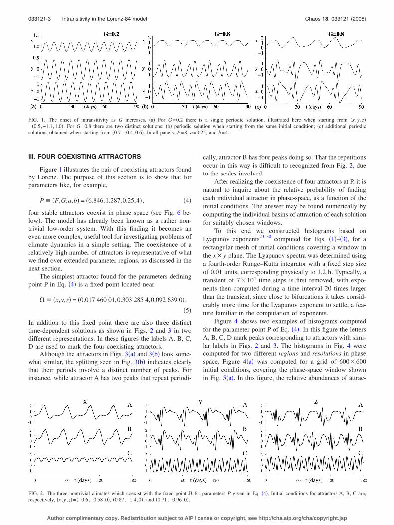
Figure 1 shows representative examples of the time-series originally studied by Lorenz, illustrating the onset ofintransitivity as the asymmetrical thermal forcing G in-creases from G=0.2 to 0.8. For G=0.2, all initial conditionseventually converge to the very regular oscillations seen onthe leftmost panel of the figure. In contrast, for G=0.8, theattractor existing originally in Fig. 1�a� evolves into the oneshown in Fig. 1�b� and a new coexisting periodic solution,shown in Fig. 1�c�, appears. In other words, the phase-spacecontains two distinct basin of attraction when G=0.8, insteadof the single basin existing for G=0.2.

033121-2 Freire et al. Chaos 18, 033121 �2008�

Author complimentary copy. Redistribution subject to AIP license or copyright, see http://cha.aip.org/cha/copyright.jsp

III. FOUR COEXISTING ATTRACTORS

Figure 1 illustrates the pair of coexisting attractors foundby Lorenz. The purpose of this section is to show that forparameters like, for example,

P � �F,G,a,b� = �6.846,1.287,0.25,4� , �4�

four stable attractors coexist in phase space �see Fig. 6 be-low�. The model has already been known as a rather non-trivial low-order system. With this finding it becomes aneven more complex, useful tool for investigating problems ofclimate dynamics in a simple setting. The coexistence of arelatively high number of attractors is representative of whatwe find over extended parameter regions, as discussed in thenext section.

The simplest attractor found for the parameters definingpoint P in Eq. �4� is a fixed point located near

� � �x,y,z� = �0.017 460 01,0.303 285 4,0.092 639 0� .

�5�

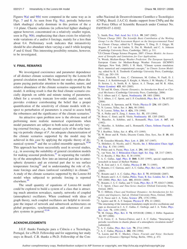
In addition to this fixed point there are also three distincttime-dependent solutions as shown in Figs. 2 and 3 in twodifferent representations. In these figures the labels A, B, C,D are used to mark the four coexisting attractors.

Although the attractors in Figs. 3�a� and 3�b� look some-what similar, the splitting seen in Fig. 3�b� indicates clearlythat their periods involve a distinct number of peaks. Forinstance, while attractor A has two peaks that repeat periodi-

cally, attractor B has four peaks doing so. That the repetitionsoccur in this way is difficult to recognized from Fig. 2, dueto the scales involved.

After realizing the coexistence of four attractors at P, it isnatural to inquire about the relative probability of findingeach individual attractor in phase-space, as a function of theinitial conditions. The answer may be found numerically bycomputing the individual basins of attraction of each solutionfor suitably chosen windows.

To this end we constructed histograms based onLyapunov exponents23–30 computed for Eqs. �1�–�3�, for arectangular mesh of initial conditions covering a window inthe x�y plane. The Lyapunov spectra was determined usinga fourth-order Runge–Kutta integrator with a fixed step sizeof 0.01 units, corresponding physically to 1.2 h. Typically, atransient of 7�104 time steps is first removed, with expo-nents then computed during a time interval 20 times largerthan the transient, since close to bifurcations it takes consid-erably more time for the Lyapunov exponent to settle, a fea-ture familiar in the computation of exponents.

Figure 4 shows two examples of histograms computedfor the parameter point P of Eq. �4�. In this figure the lettersA, B, C, D mark peaks corresponding to attractors with simi-lar labels in Figs. 2 and 3. The histograms in Fig. 4 werecomputed for two different regions and resolutions in phasespace. Figure 4�a� was computed for a grid of 600�600initial conditions, covering the phase-space window shownin Fig. 5�a�. In this figure, the relative abundances of attrac-

FIG. 1. The onset of intransitivity as G increases. �a� For G=0.2 there is a single periodic solution, illustrated here when starting from �x ,y ,z�= �0.5,−1.1,1.0�. For G=0.8 there are two distinct solutions: �b� periodic solution when starting from the same initial condition; �c� additional periodicsolutions obtained when starting from �0.7,−0.4,0.6�. In all panels: F=8, a=0.25, and b=4.

FIG. 2. The three nontrivial climates which coexist with the fixed point � for parameters P given in Eq. �4�. Initial conditions for attractors A, B, C are,respectively, �x ,y ,z�= �−0.6,−0.58,0�, �0.87,−1.4,0�, and �0.71,−0.96,0�.

033121-3 Intransitivity in the Lorenz-84 model Chaos 18, 033121 �2008�

Author complimentary copy. Redistribution subject to AIP license or copyright, see http://cha.aip.org/cha/copyright.jsp

tors A, B, C, D are 35.06%, 24.70%, 0.23%, 40.01%, respec-tively. In contrast, Fig. 4�b� was obtained for a grid of 750�750 initial conditions covering the window shown in Fig.5�b�. The relative abundances of A, B, C, D are 37.12%,21.00%, 2.15%, 39.73%, respectively. In both figures, thelargest D peak, near −1.2, corresponds to the fixed point �.Comparing the histograms in Figs. 4�a� and 4�b� one recog-nizes that the relative distribution is not much affected by thedistinct regions and distinct resolutions used to obtain them.

Figure 5 shows the very intricate structuring of the ba-sins of attraction for the parameters at point P. The basinswere easily plotted with the help of the histograms in Fig. 4.They allow us to discriminate attractors in phase space bycoloring in a similar way all exponents that fall under a givenpeak. For instance, the basins corresponding to the histo-grams in Figs. 4�a� and 4�b� are shown in Figs. 5�a� and 5�b�,respectively. The basins seen in Fig. 5 show z=0 sections ofthe phase space, indicating clearly that the four basins arevery intertwined and imply strong final state sensitivity oninitial conditions. Figure 5�a� also shows that the basins ofthe fixed point D and attractors A and B are considerably

larger than that of attractor C, essentially invisible in thisscale, and that may be easily missed under low resolution orwashed out in the presence of noise. The basin of the attrac-tor C is visible in the zoom presented in Fig. 5�b�. The basinsin Fig. 5 seem to have the Wada property, an indicator ofstrong unpredictability of the parameters in this phase.31,32

IV. INTRANSITIVITY DIAGRAMS

The purpose of this section is to present phase diagramsdiscriminating all possible climates of the Lorenz-84 model,and to characterize the abundance of intransitivity,10,11 i.e.,the abundance of multistability in parameter space. Wepresent phase diagrams showing that the several attractors

FIG. 3. Three-dimensional views of the four attractors coexisting at thepoint P defined in Eq. �4� and indicated by the white dot in Fig. 6. The fixedpoint seen in panel D is located at the point � defined in Eq. �5�.

FIG. 4. The relatively invariant volume of the basins of attraction of the fourattractors at P, determined by the second largest Lyapunov exponent for tworegions and resolutions in phase space. �a� Histogram for 600�600 initialconditions covering the window shown in Fig. 5�a�. �b� Histogram for 750�750 initial conditions covering the window shown in Fig. 5�b�; see text.

FIG. 5. �Color online� Very strong sensitivity to initial conditions illustratedby basins of attraction for a z=0 surface section of Eqs. �1�–�3�. The fourcolors represent the four attractors coexisting for parameters P, Eq. �4�,colored according to the four peaks in the histograms in Fig. 4. �a� A largewindow of phase-space; �b� magnification of the box in �a�. The letters A, B,C, D mark basins using the same labels in Figs. 2 and 3. The crosses indicateinitial conditions �x ,y ,z� leading to the attractors A, B, C, D, respectively:�−0.6,−0.58,0�, �0.87,−1.4,0�, �0.71,−0.96,0�, �0.65,−0.67,0�.

033121-4 Freire et al. Chaos 18, 033121 �2008�

Author complimentary copy. Redistribution subject to AIP license or copyright, see http://cha.aip.org/cha/copyright.jsp

discussed in the previous section exist over relatively wideregions of parameter space and describe the fourfold “foli-ated” nature of the parameter space, as induced by the initialconditions leading to individual climates �attractors�.

As it is well known, the final attractor toward which thesystem converges usually depends sensitively on the initialconditions used to start the integration.29,30 This is illustratedin Fig. 1 for G=0.8. A consequence of this fact is that phasediagrams normally contain “overlaps,” i.e., parameter re-gions where more than one attractor coexist simultaneously.Such overlap of distinct attractors is the same one facedwhen plotting bifurcation diagrams in the presence of intran-sitivity.

Figure 6 shows a phase diagram discriminating with col-ors the number of different attractors coexisting in a 600�600 window in parameter space, as indicated by the labels.The shape and volume of the coexistence regions varies con-siderably. The triangular-shaped region containing the label 4indicates the domain where four attractors coexist. The whitedot roughly at the center of the region indicates the locationof the point P of Eq. �4�.

Figure 6 was obtained by determining the boundaries ofthe parameter planes corresponding to each coexisting attrac-tor. Such boundaries were obtained by following individualattractors in all directions in parameter space, as far as pos-sible.

When performing computations for large sets of param-eters and initial conditions one normally tunes integrators toproduce reliable exponents by conducting a reasonable num-ber of tests and assuming that such tests define the quality ofall subsequent integrations.23,24 However, as it is also thecase in the computation of bifurcation diagrams,29,30 nearbifurcation boundaries there is a considerable “numericallethargy,” a pronounced increase in the transient time need toapproach the final attractor and to assure convergence ofLyapunov exponents. For these reasons, the boundaries ofthe region where four different attractors coexist in Fig. 6 arecomputationally time consuming to define accurately withhigh resolution. While we believe the overall volume andstructuring of the boundaries in Fig. 6 to be essentially cor-

rect, small gaps and fluctuations might exist along theboundaries.33–37 Therefore, boundaries should be regarded asschematic in the figure. At any rate, our present aim is toshow the existence of an extended four-climate phase, not todefine unambiguously the structure of the boundaries.

Each of the coexisting attractors coexisting in Fig. 6 hasa corresponding basin of attraction in phase space which,when properly scanned, reveals a foliated structuring of theparameter space as displayed in the four panels in Fig. 7. Inthis, and in similar figures below, we plot 600�600Lyapunov exponents on an equally spaced rectangular grid.Gray tonalities are used to represent parameter regions con-taining fixed points and other periodic motions �i.e., negativeexponents�. In contrast, yellow and red colors are used torepresent chaotic phases �i.e., positive exponents�, with redindicating exponents of larger magnitude.

When more than one attractor coexists, we selected oneof them to define the color in the figures, usually chosen tomaximize the information content of the phase diagram. Col-ors represent always exponents of largest nontrivial magni-tudes, meaning that the second largest exponent was usedwhenever the magnitude of the largest exponent was foundto be zero. Furthermore, although the same scale of colors isused for all pictures, scales were renormalized to reflect themaximum and minimum exponents present in each indi-vidual figure �instead of using a fixed color scale for allfigures�.

Altogether, we find four distinct sets of initial conditions,leading to the four parameter planes shown in Fig. 7. Theindividual panels in Fig. 7 were computed by starting from afixed arbitrary initial condition on an arbitrary boundary,here the leftmost boundary, and then proceeding by “follow-ing the attractor.”33 By this we mean to follow as much aspossible the evolution of that particular attractor found at theinitial boundary, by repeating the following expedient: �i�record the value of all variables at the end of an integrationfor a fixed set of parameters; �ii� increment parameters in-finitesimally; �iii� use the recorded values of the variables asinitial conditions to start integration for the new �incre-mented� parameters.

For the record, we mention that Fig. 6 was obtained bycombining in a single figure the results contained in the fourpanels of 7. Figure 6 results from the determination of thenumber of coexisting climates done by the analysis of theLyapunov histograms for 4�600�600 parameter pairs�F ,G�, a time-consuming numerical task.

Figure 8 presents a larger view of parameter space, ob-tained by following the attractor found on the left F=3boundary. The roughly triangular-shaped region seen in theupper left corner marks the domain of fixed points investi-gated by Lorenz.10,11 The parameter region contained insidethe box is the same considered previously in Figs. 6 and 7.The rough characterization reported by Roebber16 agreeswell with the classification presented in our Fig. 8. The verycoarse-grained classification of Roebber is by far the mostdetailed classification that we are aware of for the climates ofthe Lorenz-84 model.

As mentioned in the Introduction, while relatively wideportions of the F�G parameter plane have been considered

FIG. 6. �Color online� Intransitivity diagram in F�G space. The numbersindicate the number of distinct climates �attractors� which coexist. The whitedot marks the point P of Eq. �4�. Here a=0.25 and b=4.

033121-5 Intransitivity in the Lorenz-84 model Chaos 18, 033121 �2008�

Author complimentary copy. Redistribution subject to AIP license or copyright, see http://cha.aip.org/cha/copyright.jsp

before by a number of authors, virtually all computations sofar were done only for Lorenz’s choice of a=0.25 and b=4.The exception are the considerations of van Veen,21 in Sec.5.1, who studies the case a=0.35 and b=1.33. To check whathappens when a and b are varied systematically we per-formed one additional experiment.

Figures 9�a� and 9�b� show phase diagrams when oneconsiders variations of a and b around the values consideredoriginally by Lorenz, while maintaining F=8 and G=1 fixed.

FIG. 7. �Color online� The four pa-rameter planes A–D which overlap toproduce the diagram of the density ofattractors depicted in Fig. 6. Here andin similar figures below, fixed pointsand other periodic solutions �negativeexponents� are represented in darkshadings. Chaotic phases �positive ex-ponents� are shown in yellow and redcolors �lighter shadings�. Crossesmark the point P of Eq. �4�. Here a=0.25 and b=4.

FIG. 8. �Color online� Global view of the F�G plane discriminating regu-lar phases �shown in dark shadings� and chaotic phases �in color�. Thechaotic phase is riddled with substructurings and accumulations with char-acteristic scaling properties �Ref. 35�. The box marks the parameter windowshown in Figs. 6 and 7. Here a=0.25 and b=4.

FIG. 9. �Color online� Phase diagrams in a�b space when fixing F=8 andG=1. The parameters studied by Lorenz and others are a=0.25, b=4, indi-cated by the cross. �a� Global view, showing predominance of periodic so-lutions, represented by the dark shadings, proportional to the magnitude ofthe exponents. �b� Zoom of the box in �a�, the region containing chaoticsolutions �lighter yellow/red shadings�.

033121-6 Freire et al. Chaos 18, 033121 �2008�

Author complimentary copy. Redistribution subject to AIP license or copyright, see http://cha.aip.org/cha/copyright.jsp

Figures 9�a� and 9�b� were computed in the same way as inFigs. 7 and 8. As seen from Fig. 9�a�, periodic behaviors�dark shadings� clearly dominate in this portion of the a�b plane. Chaotic solutions �in yellow/red lighter shadings�appear however, concentrated on a relatively smaller region,seen in Fig. 9�b�, emphasizing that chaos exists for relativelywide variations of a and/or b forcings, mainly for a less thanabout 0.4. Preliminary work indicates that intransitivityshould be also abundant when varying a and b while keepingF and G fixed. This interesting possibility remains, however,to be investigated.

V. FINAL REMARKS

We investigated coexistence and parameter dependenceof all distinct climate scenarios supported by the Lorenz-84general circulation model. We based our study on phase dia-grams paying particular attention to the number, nature, andrelative abundance of the climate scenarios supported by themodel. A striking result is that the final climate scenario cru-cially depends on subtle and minute tuning of parameters.Albeit for a severely truncate low-order model, our workprovides evidence corroborating the belief that a properquantification of the sensitivity of climate models with re-spect to perturbation of parameters is crucial to assess boththe robustness and the significance of the climate scenarios.3

An attractive open problem now is the obvious need ofperforming more realistic numerical experiments whenmodel parameters are subject to both noise and slowly vary-ing external forcings, e.g., the annual cycle of the solar heat-ing via periodic change of F. An adequate characterization ofthe climate scenarios supported by the model may beachieved in this case by applying the ergodic theory of dy-namical systems38 and the so-called ensemble approach.39,40

This approach has been successfully used in several studies,e.g., in assessing the suitability of general circulation modelsfor making seasonal predictions,41 in separating the variabil-ity of the atmospheric flow into an internal part due to atmo-spheric dynamics and an external part due to sea surfacetemperature forcing42 and in understanding the role of cli-mate forcings and chaos �unforced variability� in climate.43

A study of the climate scenarios supported by the Lorenz-84model when subjected to periodic forcing is reportedelsewhere.44

The small quantity of equations of Lorenz-84 modelcould be explored to build a system of a class that is attract-ing much attention nowadays, namely, networks of coupled�atmospheric� oscillators. When combined with ideas ofgraph theory, such coupled oscillators are helpful to investi-gate the impact of network and subnetwork architectures onglobal properties, synchronization, and coherence of com-plex systems in general.45,46

ACKNOWLEDGMENTS

J.G.F. thanks Fundação para a Ciência e a Tecnologia,Portugal, for a Ph.D. Fellowship and for supporting her studystays in Brazil. C.B. thanks a Ph.D. Fellowship of the Con-

selho Nacional de Desenvolvimento Científico e Tecnológico�CNPq�, Brazil. J.A.C.G. thanks support from CNPq and theAir Force Office of Scientific Research under Contract No.FA9550-07-1-0102.

1L. Smith, Proc. Natl. Acad. Sci. U.S.A. 99, 2487 �2002�.2Climate Change 2001: The Scientific Basis Contribution of the WorkingGroup I to the Third Assessment Report on the Intergovernmental Panelon Climate Change, edited by T. Houghton, Y. Ding, D. J. Griggs, M.Noguer, P. J. van der Linden, X. Dai, K. Maskell, and C. A. Johnson�Cambridge University Press, Cambridge, 2001�, p. 511.

3US Climate Change Science Program, 2007: Climate Models: An Assess-ment of Strengths and Limitations for User Applications.

4A. Woods, Medium-Range Weather Prediction: The European Approach,European Centre for Medium-Range Weather Forecasts �ECMWF��Springer, New York, 2005�; J. H. Hack, “Climate system simulation:Basic numerical and computational concepts,” in Climate System Model-ing, edited by K. E. Trenberth �Cambridge University Press, Cambridge,1992�, pp. 283–318.

5D. A. Stainforth, T. Aina, C. Christensen, M. Collins, N. Faull, D. J.Frame, J. A. Kettleborough, S. Knight, A. Martin, J. M. Murphy, C. Piani,D. Sexton, L. A. Smith, R. A. Spicer, A. J. Thorpe, and M. R. Allen,Nature �London� 433, 403 �2005�.

6T. Tel and M. Gruiz, Chaotic Dynamics, An Introduction Based on Clas-sical Mechanics �Cambridge University Press, Cambridge, 2006�.

7D. J. Albers and J. C. Sprott, Nonlinearity 19, 1801 �2006�.8D. J. Albers, J. C. Sprott, and J. P. Cruchfield, Phys. Rev. E 74, 057201�2006�.

9V. Lucarini, A. Speranza, and R. Vitolo, Physica D 234, 105 �2007�.10E. N. Lorenz, Tellus, Ser. A 36A, 98 �1984�.11E. N. Lorenz, Tellus, Ser. A 42A, 378 �1990�.12R. A. Pielke and X. Zeng, J. Atmos. Sci. 51, 155 �1994�.13H. Broer, C. Simó, and R. Vitolo, Nonlinearity 15, 1205 �2002�.14C. Masoller, A. Schifino, and L. Romanelli, Phys. Lett. A 167, 185

�1992�.15C. Masoller, A. Schifino, and L. Romanelli, Chaos, Solitons Fractals 6,

357 �1995�.16P. J. Roebber, Tellus, Ser. A 47A, 473 �1995�.17H. W. Broer and R. Vitolo, Discrete Contin. Dyn. Syst., Ser. B 10, 401

�2008�.18J. M. González-Miranda, Phys. Lett. A 233, 347 �1997�.19A. Shilnikov, G. Nicolis, and C. Nicolis, Int. J. Bifurcation Chaos Appl.

Sci. Eng. 5, 1701 �1995�.20V. Pelino and A. Pasini, Phys. Lett. A 291, 389 �2001�.21L. van Veen, Int. J. Bifurcation Chaos Appl. Sci. Eng. 13, 2117 �2003�.22C. G. Rossby, J. Mar. Res. 5, 38 �1939�.23J. A. C. Gallas, Appl. Phys. B B60, S-203 �1995�, special supplement,

festschrift in honor of Herbert Walther.24A. R. Zeni and J. A. C. Gallas, Physica D 89, 71 �1995�.25C. Bonatto, J. C. Garreau, and J. A. C. Gallas, Phys. Rev. Lett. 95, 143905

�2005�.26C. Bonatto and J. A. C. Gallas, Phys. Rev. E 75, 055204�R� �2007�.27C. Bonatto and J. A. C. Gallas, Philos. Trans. R. Soc. London, Ser. A 366,

505 �2008�; Phys. Rev. Lett. 101, 054101 �2008�.28C. Bonatto, J. A. C. Gallas, and Y. Ueda, Phys. Rev. E 77, 026217 �2008�.29J. C. Sprott, Chaos and Time-Series Analysis �Oxford University Press,

Oxford, 2003�.30R. C. Hilborn, Chaos and Nonlinear Dynamics: An Introduction for Sci-

entists and Engineers, 2nd ed. �Oxford University Press, Oxford, 2000�.31H. E. Nusse and J. A. Yorke, Science 271, 1376 �1996�.32J. Aguirre and M. A. F. Sanjuan, Physica D 171, 41 �2002�.33The structuring of the innermost boundaries might involve oscillations and

gaps as discussed in J. A. C. Gallas, C. Grebogi, and J. A. Yorke, Phys.Rev. Lett. 71, 1359 �1993�.

34H. M. Osinga, Phys. Rev. E 74, 035201�R� �2006�; J. Differ. Equations12, 997 �2006�.

35J. G. Freire, C. A. Torrico-Chávez, and J. A. C. Gallas, “Structuring ofperiodic waveforms in chaotic phases of a atmospheric circulation model”�submitted�.

36J. A. C. Gallas, Phys. Rev. Lett. 70, 2714 �1993�.37J. A. C. Gallas, Physica A 202, 196 �1994�.38A. Lasota and M. C. Mackey, Chaos, Fractals and Noise: Stochastic

Aspects of Dynamics �Springer-Verlag, Berlin, 1994�, p. 472.

033121-7 Intransitivity in the Lorenz-84 model Chaos 18, 033121 �2008�

Author complimentary copy. Redistribution subject to AIP license or copyright, see http://cha.aip.org/cha/copyright.jsp

39C. E. Leith, Mon. Weather Rev. 102, 409 �1974�; Nature �London� 276,352 �1978�.

40E. S. Epstein, Tellus 21, 739 �1969�.41A. Kumar, M. Hoerling, M. Ji, A. Leetmaa, and P. Sardeshmukh, J. Clim.

9, 115 �1996�.42A. Harzallah and R. Sadourny, J. Clim. 8, 474 �1995�.43J. Hansen, M. Sato, R. Ruedy, A. Lacis, K. Asamoah, K. Beckford, S.

Borenstein, E. Brown, B. Cairns, B. Carlson, B. Curran, S. de Castro, L.Druyan, P. Etwarrow, T. Ferede, M. Fox, D. Gaffen, J. Glascoe, H. Gor-don, S. Hollandsworth, X. Jiang, C. Johnson, N. Lawrence, J. Lean, J.Lerner, K. Lo, J. Logan, A. Luckett, M. P. McCormick, R. McPeters, R.

Miller, P. Minnis, I. Ramberran, G. Russell, P. Russell, P. Stone, I. Tegen,S. Thomas, L. Thomason, A. Thompson, J. Wilder, R. Willson, and J.Zawodny, J. Geophys. Res. 102, 25679, DOI: 10.1029/97JD01495�1997�.

44J. G. Freire, C. A. L. Pires, C. DaCamara, and J. A. C. Gallas �submitted�.45P. G. Lind, J. A. C. Gallas, and H. J. Herrmann, Phys. Rev. E 70, 056207

�2004�; P. G. Lind, A. Nunes, and J. A. C. Gallas, Physica A 371, 100�2006�.

46A. A. Tsonis and P. J. Roebber, Physica D 333, 497 �2004�; P. J. Roebberand A. A. Tsonis, J. Atmos. Sci. 62, 3818 �2005�.

033121-8 Freire et al. Chaos 18, 033121 �2008�

Author complimentary copy. Redistribution subject to AIP license or copyright, see http://cha.aip.org/cha/copyright.jsp