Abstract To improve our understanding of the

mechanism causing the 8.2 ka BP event, we inves-

tigated the response of ocean circulation in the

ECBilt-CLIO-VECODE (Version 3) model to various

freshwater fluxes into the Labrador Sea. Starting from

an early Holocene climate state we released freshwater

pulses varying in volume and duration based on pub-

lished estimates. In addition we tested the effect of a

baseline flow (0.172 Sv) in the Labrador Sea to account

for the background-melting of the Laurentide ice-sheet

on the early Holocene climate and on the response of

the overturning circulation. Our results imply that the

amount of freshwater released is the decisive factor in

the response of the ocean, while the release duration

only plays a minor role, at least when considering the

short release durations (1, 2 and 5 years) of the applied

freshwater pulses. Furthermore, the experiments with a

baseline flow produce a more realistic early Holocene

climate state without Labrador Sea Water formation.

Meltwater pulses introduced into this climate state

produce a prolonged weakening of the overturning

circulation compared to an early Holocene climate

without baseline flow, and therefore less freshwater is

needed to produce an event of similar duration.

1 Introduction

During the early Holocene from 11.5 to 7 cal ka BP

(hereafter ka BP), the remaining glacial ice-sheets

melted under the warm climate conditions. Due to

regional geography in North America, part of the

meltwater collected in huge proglacial lakes south of

the retreating Laurentide Ice-Sheet (LIS), the so-called

Laurentide lakes. The remnant LIS formed a massive

ice-dam, which prevented the lakes from draining into

the North Atlantic Ocean (e.g. Upham 1896; Veillette

1994; Clarke et al. 2004). Between 9 and 8 ka BP,

collapse of the ice-dam became unavoidable, thereby

releasing a huge amount of meltwater into the Hudson

Bay.

The timing of the collapse of the ice-dam and the

subsequent draining of the Laurentide lakes is esti-

mated at ~8.47 ka BP (Barber et al. 1999), and con-

sidering dating uncertainties, this coincides with the

start of the most pronounced cold period recorded in

the North Atlantic area, the so called 8.2 ka BP event

(e.g. Alley et al. 1997; Barber et al. 1999). Several

investigators linked the two events, suggesting that the

drainage of the Laurentide lakes caused the 8.2 ka BP

event (e.g. von Grafenstein et al. 1998; Klitgaard-

Kristensen et al. 1998; Barber et al. 1999). The pro-

posed mechanism is that the freshwater slowed down

the Meridional Overturning Circulation (MOC) by

A. P. Wiersma (&) Æ H. RenssenFaculty of Earth and Life Sciences, Vrije UniversiteitAmsterdam, De Boelelaan 1085, 1081 HV Amsterdam,The Netherlandse-mail: ane.wiersma@falw.vu.nl

H. Goosse Æ T. FichefetInstitut d’Astronomie et de Geophysique George Lemaıtre,Universite Catholique de Louvain, Chemin du Cyclotron 2,1348 Louvain-la-Neuve, Belgium

Clim Dyn (2006) 27:831–849

DOI 10.1007/s00382-006-0166-0

123

Evaluation of different freshwater forcing scenarios for the 8.2 kaBP event in a coupled climate model

A. P. Wiersma Æ H. Renssen Æ H. Goosse ÆT. Fichefet

Received: 19 January 2006 / Accepted: 2 June 2006 / Published online: 22 July 2006� Springer-Verlag 2006

preventing dense water to sink in the North Atlantic

Ocean and thereby reducing the northward heat

transport to the North Atlantic region. Such a collapse

of the MOC is also observed during Heinrich events

(Keigwin and Lehman 1994; Elliot et al. 2002), and in

modelling studies in which the modern North Atlantic

is perturbed with freshwater (e.g. Stocker and Wright

1991; Manabe and Stouffer 1995, 1997; Vellinga and

Wood 2002).

In recent years, widely varying estimates of the in-

volved freshwater pulse have been published (Table 1),

ranging from 0.3 to 5.0 · 1014 m3. A comprehensive

study by Leverington et al. (2002) produced an estimate

of 1.63 · 1014 m3 based on bathymetric models. To

constrain the magnitude and duration of the flood,

Clarke et al. (2004) simulated flood hydrographs for

lake discharge for different drainage routes and from

different filling levels, and found that the draining of the

Laurentide lakes had a typical duration of less than a

year with peak discharge rates up to 9 Sv (1 Sv =

106 m3/s). The total water volume available for drain-

age for the different drainage routes ranged from

0.40 · 1014 to 1.51 · 1014 m3. Surprisingly, several

hydrographs revealed a multi-pulse structure and in

none of the experiments the lakes drained completely.

Even in the scenario with the largest drained volume,

less than half of the total available volume of the lake

drained. However, Clarke et al. (2004) only accounted

for subglacial outburst flooding. They could not rule out

physical failure of the LIS, collapse of the ice roof of

subglacial channels and a supraglacial flood mechanism

as additional freshwater sources (Clarke et al. 2005;

Sharpe 2005). Consequently, the released volume and

drainage duration may have been larger than suggested

by Clarke et al. (2004).

Complete or partial physical failure of the LIS

would have led to the release of an additional volume

of ice, in addition to the lake water. Based on maps of

Dyke and Prest (1989) and von Grafenstein et al.

(1998) even suggested that one third of the LIS may

have been released into the Labrador Sea as floating

ice and roughly estimates that 5 · 1014 m3 of meltwater

from the lakes and the ice-sheet was released. How-

ever, Tornqvist et al. (2004) showed recently that the

maximum sea-level rise following the lake drainage is

1.19 m, implying that the total volume of meltwater

and ice cannot have exceeded 4.3 · 1014 m3. Still, de-

spite this maximum constrain, the actual volume of

meltwater that was released remains highly uncertain

(Table 1), especially since the contribution of the LIS,

from which a substantial part disappeared between 7.8

and 7.2 14C ka BP (~8.6–8.0 ka BP, Dyke 2003), is still

unclear. On the floor of the Hudson Bay, however,

there is evidence for drifting icebergs during the dis-

charge: a large area with iceberg scours is present,

probably originating from grounded icebergs that

were mobilized by fast-flowing water (Josenhans and

Zevenhuizen 1990; Dyke 2003). In addition, peaks in

ice-rafted detritus (IRD) in several marine cores in the

Atlantic Ocean around 8.2 ka BP (e.g. Bond et al.

2001; Moros et al. 2004) suggest the drifting of ice-

bergs, but on the other hand these IRD peaks may also

reflect the 8.2 ka BP cooling.

When the Laurentide lakes drained in the early

Holocene, the Atlantic Ocean circulation was different

from the present. From micropaleontological data and

stable isotopes on both planktonic and benthic fora-

minifera, Hillaire-Marcel et al. (2001) concluded that

deep-water formation in the Labrador Sea was absent

during the last glacial cycle and only started at

7 ka BP. This means that Labrador Sea Water (LSW)

formation was probably absent at the time of the lake

discharge around 8.47 ka BP. In a modelling study

focused on Holocene North Atlantic deep-water for-

mation, Renssen et al. (2005a) performed an experi-

ment forced only by changes in orbital forcing and

atmospheric trace gas concentrations for the last

9,000 years. They found that the LSW formation was

weaker in the early Holocene than at present. How-

ever, in this study, a complete shutdown of LSW for-

mation in the early Holocene was not simulated under

the imposed forcings. This was probably related to a

relatively high surface salinity in the Labrador Sea in

the early Holocene, since the effect of the melting LIS

(i.e. the associated freshwater flux) was not included in

the experiments (Renssen et al. 2005a). The latter

conclusion is consistent with Cottet-Puinel et al.

(2004), who simulated an early Holocene shutdown of

Table 1 Estimates of the volume of freshwater that was releasedduring the collapse of the remnant Laurentide ice-sheet previousto 8.2 ka BP

Authors Freshwatervolume(1014 m3)

von Grafenstein et al. (1998) 5de Vernal (1997) 1.2Leverington et al. (2002) 1.63Barber et al. (1999) ~2Tornqvist et al. (2004) < 4.3Veillette (1994) ~2.28Clarke et al. (2004) 0.279–0.708

Modelling papersBauer et al. (2004) 1.6Renssen et al. (2001) 4.67This paper 1.63

3.264.89

832 A. P. Wiersma et al.: Evaluation of different freshwater forcing scenarios (2006) 27:831–849

123

LSW formation in a transient model run including the

freshwater runoff of the LIS.

Recently, several attempts have been made to sim-

ulate the 8.2 ka BP event. Renssen et al. (2001, 2002)

introduced pulses of freshwater into the Labrador Sea

under early Holocene boundary conditions, using

Version 2 of the ECBilt-CLIO climate model. A sce-

nario with a fresh water pulse of 4.67 · 1014 m3 during

20 years resulted in a cold period comparable to the

8.2 ka BP event as reconstructed from proxy-evidence

(Wiersma and Renssen 2006). Later, Bauer et al.

(2004) simulated the event with the CLIMBER-2

model, by introducing a 2-year pulse of 1.6 · 1014 m3

fresh-water into the North Atlantic Ocean between 50

and 70�N, also in an early Holocene climate. The

experiment produced a short-term cooling of 20-year

duration. Additionally, Bauer et al. (2004) experi-

mented with a freshwater flux representing the back-

ground melting LIS (the so-called baseline flow). This

baseline flow weakened the MOC, which promoted

collapse of the NADW formation after introducing the

same freshwater pulse of 1.6 · 1014 m3, in some sce-

narios resulting in a cooling lasting two centuries.

Altogether, the specific conditions that probably led

to the 8.2 ka BP event remain uncertain. The latest

estimates suggest that the released meltwater volume

during the collapse of the LIS was between

0.279 · 1014 (Clarke et al. 2004) and 4.3 · 1014 m3

(Tornqvist et al. 2004) and that the release duration

was short, and estimates range from between 1 and

10 years (Licciardi et al. 1999) to even less than a year

(Barber et al. 1999; Clarke et al. 2004).

Knowing these specific conditions for the 8.2 ka BP

event provides crucial information on the sensitivity of

the MOC to perturbations (e.g. Schlessinger 2005). In

this study, we investigate the influence of varying

magnitude and duration of the freshwater pulse on the

response of the MOC in Version 3 of the ECBilt-

CLIO-VECODE model while previous modelling

studies experimented with a constant volume (Bauer

et al. 2004), and unrealistic release durations (i.e.

10 years or more, Renssen et al. 2001, 2002). In con-

trast to the previous study of Bauer et al. (2004), our

model allows us to investigate the spatial response of

the ocean to this forcing. Furthermore, we investigate

the influence of a baseline flow due to the LIS melting

on the early Holocene climate as in Bauer et al. (2004),

and its influence on the MOC’s response to the varying

freshwater perturbations. This provides information on

the sensitivity of the MOC to these factors (i.e. fresh-

water volume, discharge rate, baseline flow or initial

conditions) as well as their share in the evolution of the

8.2 ka BP event.

2 The ECBilt-CLIO-VECODE model

We have performed our experiment with Version 3 of

the ECBilt-CLIO-VECODE model, a global, three-

dimensional climate model of intermediate complexity.

The model consists of an oceanic, sea-ice, atmospheric

and vegetation component. The atmospheric compo-

nent is Version 2 of ECBilt, a spectral quasi-geo-

strophic model with three levels and T21-resolution

developed at the Koninklijk Nederlands Meteorologi-

sch Instituut (KNMI) (Opsteegh et al. 1998). ECBilt

includes a representation of the hydrological cycle and

simple parameterizations of the diabatic heating pro-

cesses. Cloudiness is prescribed according to present-

day climatology (Rossow et al. 1996) and a dynamically

passive stratospheric layer is included. As an extension

to the quasi-geostrophic equations, an estimate of the

neglected terms in the vorticity and thermodynamic

equations is incorporated as a temporally and spatially

varying forcing (Opsteegh et al. 1998). This forcing is

computed from the diagnostically derived vertical

motion field, leading to a considerable improvement of

the simulation of the Hadley circulation and resulting

in a drastic improvement of the strength and position

of the jet stream and transient eddy activity. The

hydrological cycle is closed over land by using a bucket

for soil moisture. Each bucket is connected to a nearby

oceanic gridcell to define river runoff. Accumulation

of snow occurs in case of precipitation in areas with

below 0�C surface temperature. Greenhouse gases are

incorporated directly into the model, and not as

equivalent CO2.

The sea-ice—ocean component is CLIO (Goosse

and Fichefet 1999), a primitive-equation free-surface

ocean general circulation model (OGCM) (Dele-

ersnijder and Campin 1995; Campin and Goosse 1999)

coupled to a comprehensive sea-ice model with a rep-

resentation of both thermodynamic and dynamic pro-

cesses (Fichefet and Morales Maqueda 1997) that was

developed at Universite Catholique de Louvain

(Goosse and Fichefet 1999). The ocean model includes

a detailed formulation of boundary layer mixing based

on Mellor and Yamada’s (1982) level-2.5 turbulence

closure scheme (Goosse et al. 1999) and a parameter-

ization of density-driven down-slope flows (Campin

and Goosse 1999). The sea-ice model takes into ac-

count the heat capacity of the snow—ice system, the

storage of latent heat in brine pockets trapped inside

the ice, the effect of the sub-grid scale snow and ice

thickness distributions on sea-ice thermodynamics, the

formation of snow ice under excessive snow loading

and the existence of leads within the ice cover. Ice

dynamics are calculated by assuming that sea ice

A. P. Wiersma et al.: Evaluation of different freshwater forcing scenarios (2006) 27:831–849 833

123

behaves as a two-dimensional viscous-plastic contin-

uum. The horizontal resolution of CLIO is 3� latitude

by 3� longitude, and there are 20 unequally spaced

vertical levels in the ocean.

The vegetation module VECODE, a dynamic global

vegetation model developed at the Potsdam Institut fur

Klimafolgenforschung (PIK) (Brovkin et al. 2002), was

recently coupled to ECBilt-CLIO. VECODE simulates

dynamics of two main terrestrial plant functional types,

trees and grasses, as well as desert (bare soil),

in response to climate change. Within ECBilt-CLIO-

VECODE, simulated vegetation changes affect only

the land-surface albedo, and have no influence on other

processes, e.g. evapotranspiration or roughness length.

Compared to earlier versions, the present model

simulates a climate, i.e. closer to modern observations.

The most important improvements in the new version

are a new land surface scheme that takes into account

the heat capacity of the soil, and the use of isopycnal

diffusion as well as the Gent and McWilliams param-

eterization to represent the effect of meso-scale eddies

in the ocean (Gent and McWilliams 1990). The climate

sensitivity of ECBilt-CLIO is about 0.5�C/(W/m2),

which is at the lower end of the range [typically 0.5–1�/

(W/m2)] found in most coupled climate models (Cu-

basch et al. 2001). The only flux correction required in

ECBilt-CLIO is an artificial reduction of precipitation

over the Atlantic and Arctic Oceans, and a homoge-

neous distribution of the removed amount of fresh-

water over the Pacific Ocean (Goosse et al. 2001).

Version 3 of the ECBilt-CLIO model was recently

applied by Knutti et al. (2004) to study the impact of

freshwater discharges on the climate during the last

glacial stage, but also in experiments investigating

Holocene climate evolution (e.g. Renssen et al. 2005a, b)

and in studies covering the last millennium (e.g.

Goosse et al. 2005). Version 2 of the model was used

earlier for the simulation of the 8.2 ka BP event

(Renssen et al. 2001, 2002) and a variety of other

applications, i.e. to simulate aspects of the present-day

climate (Goosse et al. 2001, 2003), natural variability of

the modern climate (Goosse et al. 2002) and future

climate evolution (Goosse and Renssen 2001; Schaef-

fer et al. 2002). The improvements and updates in

model Version 3 lead to important differences with

model Version 2 that was used by Renssen et al. (2001,

2002) to study the 8.2 ka BP event. In contrast to

Version 2, when run with modern forcings, the new

version simulates deep convection in the Labrador Sea

in agreement with observational estimates, and also the

strength of overturning in the Greenland–Iceland–

Norwegian (GIN) seas is greatly reduced to more realistic

values of < 4 Sv (compared to ~17 Sv in Version 2).

Under pre-industrial climate conditions, the maximum of

the North Atlantic overturning circulation is in present

model version ~27 and ~13 Sv of NADW is exported

southward at 20�S and the meridional heat transport at

30�S is 0.33 PW.

More detailed information about ECBilt-CLIO-

VECODE and its climatology can be found on the

models website (http://www.knmi.nl/onderzk/CKO/

ecbilt.html). In particular, a description of the differ-

ences between ECBilt-CLIO Versions 2 and 3 is

also available on this website (http://www.knmi.nl/

onderzkCKO/differences.html).

3 Early Holocene reference climate

3.1 Experimental setup

To simulate the early Holocene climate state, we ad-

justed several boundary conditions to their 8.5 ka BP

values. Atmospheric greenhouse gas concentrations

were adjusted to their 8.5 ka BP values inferred

from ice-cores analyses by Raynaud et al. (2000)

(i.e. CO2 = 261 ppbv, CH4 = 650 ppbv and N2O =

270 ppbv). Orbital parameters were adjusted to rep-

resent 8.5 ka BP insolation conditions (Berger and

Loutre 1991; Berger 1992), with higher insolation val-

ues in the northern hemisphere in boreal summer and

lower insolation values in boreal winter compared to

present-day values. We accounted for a remnant LIS

by lowering surface albedo and increasing elevation of

the concerned gridcells according to the Peltier (1994)

reconstruction (assuming a deglaciated Hudson Bay).

The model was run for 850 years with these

8.5 ka BP boundary conditions until it reached a

quasi-equilibrium in the deepest ocean layer

(dT/dt < 0.0002�C/100 years). The results from the

last 100 years of this experiment are used in this paper

to analyse the early Holocene quasi-equilibrium

climate state without baseline flow (EHequi).

In addition to this early Holocene quasi-equilibrium

state, we investigated the effect of the background LIS

melting by introducing a baseline flow (Bauer et al.

2004) into the Labrador Sea (ECBilt gridcell centred

around 53.5�N and 50.5�W), starting from EHequi.

Before the lake discharge this baseline flow is recon-

structed to have amounted to 0.15 Sv, increasing to

0.172 Sv after the discharge (Licciardi et al. 1999; Teller

et al. 2002). We used the latter value as the baseline

flow magnitude during the course of this experiment.

The model was run for 900 years in this configuration

until the temperature of the deepest ocean layer was

quasi-stable (dT/dt < 0.01�C/100 years). The results

834 A. P. Wiersma et al.: Evaluation of different freshwater forcing scenarios (2006) 27:831–849

123

from the last 100 years of this experiment are used in

this paper to analyse the early Holocene quasi-equi-

librium climate state with a baseline flow (EHBLF). It

should be noted that experiments including a baseline

flow into the Labrador Sea are not considered equilib-

rium climate states, since we add water to the ocean,

which slowly reduces salinity. However, this is analo-

gous to the early Holocene situation of a melting rem-

nant ice-sheet. A consequence is, that in the EHBLF

experiments, the global mean ocean salinity is 0.1 psu

lower than in the EHequi experiments at the end of the

early Holocene equilibrium runs.

3.2 Impact of the baseline flow on the early

Holocene climate

In the EHequi experiments, deep convection occurs in

the Nordic Seas, the Irminger Sea and in the Labrador

Sea (Fig. 1a). In this state, the maximum North

Atlantic overturning is 24 Sv (Fig. 1b). This state is

very close to the one simulated by the model for pre-

industrial conditions, with only a weak decrease of the

intensity of the MOC for the early Holocene. The

introduction of the baseline flow in the early Holocene

climate causes the Labrador Sea convection depth to

greatly decrease by more than 500 m in February

(Fig. 1c, e) and subsequently LSW formation to almost

shutdown. This is consistent with proxy-data suggesting

no LSW formation during the early Holocene (Hil-

laire-Marcel et al. 2001). The near absence of LSW

formation as a result of the baseline flow causes a

reduction in maximum North Atlantic overturning of

more than 7 Sv and a shallower NADW cell (Fig. 1d, f).

Overturning in the GIN Seas is almost unaffected by

the baseline freshwater input in the Labrador Sea, and

decreases from 3.3 Sv in EHequi to 3.2 Sv in EHBLF.

In terms of NADW export, only 10.8 Sv crosses at 20�S

in EHBLF compared to 13.8 Sv in EHequi.

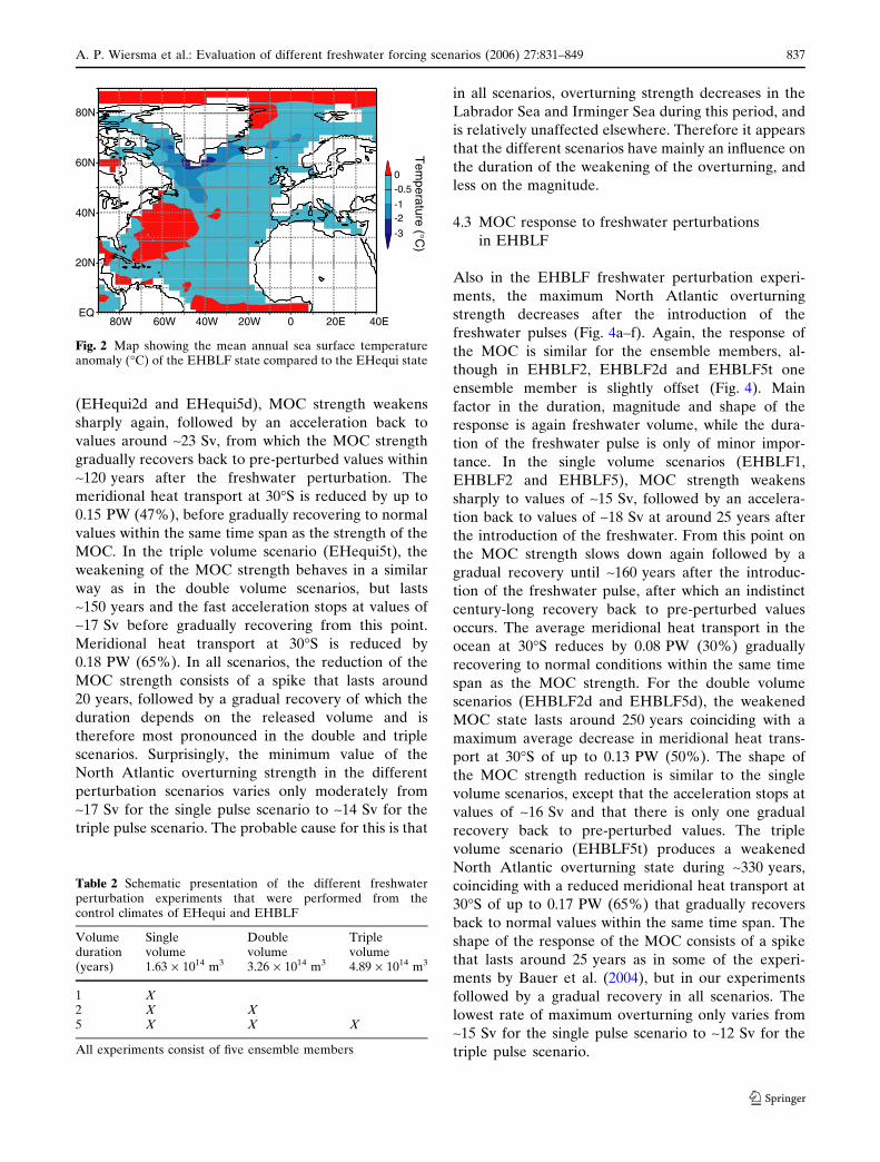
The reduced overturning in the North Atlantic leads

to a decrease in meridional heat transport, at 30�S a

decrease of 21% from 0.33 PW in EHequi to 0.26 PW

in EHBLF. Since deep convection almost ceased in the

Labrador Sea, the effect of this decreased heat flux is

mostly visible here, leading to ~2�C cooler conditions

(Fig. 2).

4 Freshwater perturbation experiments

4.1 Experimental setup

We perturbed both early Holocene climate states

(EHequi and EHBLF) by releasing freshwater pulses

into the Labrador Sea (ECBilt gridcell centred around

53.5�N and 50.5�W), varying in volume and duration. It

is assumed that the temperature of the discharged

freshwater is identical to the sea surface temperature at

the spot of discharge. Table 2 summarizes the different

performed experiments schematically. The ‘‘single

volume’’ of 1.63 · 1014 m3 is based on the estimate by

Leverington et al. (2002). The ‘‘double volume’’ cor-

responds to a total volume of 3.26 · 1014 m3 to take

into account that some ice could have been released

too because of the freshwater discharge. Note that

the ‘‘triple volume’’ scenario of 4.89 · 1014 m3 is an

amount that even exceeds the maximum set by

Tornqvist et al. (2004) and is not realistic for an

8.2 ka BP event simulation, but it is used here to assess

how close the Atlantic overturning is to a collapse or

shift to an intermediate stable state. It is also near the

value used by Renssen et al. (2001, 2002). Every

experiment (with same volume and duration of the

freshwater pulse) was performed five times (i.e. five

ensemble members), each with different initial condi-

tions, which were obtained by taking samples every

10 years from a continuation of the early Holocene

experiment. The ensemble members have been

labelled ‘‘a’’ to ‘‘e’’. After the freshwater perturbation,

the experiments were continued in the configuration of

before the pulse.

In the next paragraphs, we will first describe the

results of the freshwater perturbation experiments of

the EHequi climate state, then the freshwater pertur-

bations of the EHBLF climate state and finish with a

comparison between the experiments. We describe the

ensemble mean of the different experiments, implying

that the variability is averaged out and that the maxi-

mum magnitude of the different ensembles is mostly

larger than the mentioned ensemble mean values.

4.2 MOC response to freshwater perturbations

in EHequi

In all experiments, the maximum North Atlantic

overturning weakens sharply after the introduction of

the freshwater pulses (Fig. 3a–f). In contrast to earlier

studies however (Renssen et al. 2001, 2002; Bauer et al.

2004), the different ensemble members show similar

responses of the strength of the MOC, which suggests

that the forcing implied by the freshwater does not

push the MOC over a threshold that could cause a shift

to an intermediate stable state. This results in a more

predictable response of the strength of the MOC to

the freshwater perturbations, compared to Renssen

et al. (2001, 2002) and Bauer et al. (2004), where the

timing of recovery from the intermediate stable was

A. P. Wiersma et al.: Evaluation of different freshwater forcing scenarios (2006) 27:831–849 835

123

unpredictable. Furthermore, the response of the

strength of the MOC in experiments in which an equal

volume of freshwater is released (i.e. Fig. 3a, b and d;

Fig. 3c and e) is comparable, regardless of the duration

of the pulse. The shape of the weakened state of the

strength of the MOC in the single volume scenarios

(EHequi1, EHequi2 and EHequi5) consists of an

immediate sharp reduction, followed by a fast accel-

eration back to near-normal values around the year

125, before gradually recovering to pre-perturbed val-

ues within 100 years. This weakening leads to an

average decrease in meridional heat transport at 30�S

of up to 0.1 PW (30%) that gradually recovers within

the same time span. In the double volume scenarios

80N

60N

40N

20N

EQ80W 60W 40W 20W 0 20E 40E

80N

60N

40N

20N

EQ80W 60W 40W 20W 0 20E 40E

80N

60N

40N

20N

EQ80W 60W 40W 20W 0 20E 40E

60S 30S EQ 30N 60N

0

500

1000

1500

2000

2500

3000

3500

4000

4500

5000

5500

0 36 9

12

15

2118

24

1512

963

0

-3-6

-30

-6

36

9

1815

1212

6

30

-3

96

30

-6-6

-30

9

630

60S 30S EQ 30N 60N

0

500

1000

1500

2000

2500

3000

3500

4000

4500

5000

5500

-3

-3

-2-1

-4

-5

-3-4

-4

-5-6

-7

0

-2

-1

-2

0

0

-6

-5

0

500

1000

1500

2000

2500

3000

3500

4000

4500

5000

5500 60S 30S EQ 30N 60N

100

200

300

400

500

600

700

800

900

1000

1100

1200

-50

-100

-150

-200

-250

-300

-350

-400

-450

-500

100

200

300

400

500

600

700

800

900

1000

a) b)

c) d)

e) f)

Convection depth (m

)C

onvection depth (m)

Convection depth (m

)

Dep

th (

m)

Dep

th (

m)

Dep

th (

m)

Fig. 1 Mean February convection depth (m) (left) and the annual mean maximum overturning streamfunction (Sv) for the initial earlyHolocene climate states (right) for a, b EHequi, c, d EHBLF and e, f the difference between the two (EHBLF minus EHequi)

836 A. P. Wiersma et al.: Evaluation of different freshwater forcing scenarios (2006) 27:831–849

123

(EHequi2d and EHequi5d), MOC strength weakens

sharply again, followed by an acceleration back to

values around ~23 Sv, from which the MOC strength

gradually recovers back to pre-perturbed values within

~120 years after the freshwater perturbation. The

meridional heat transport at 30�S is reduced by up to

0.15 PW (47%), before gradually recovering to normal

values within the same time span as the strength of the

MOC. In the triple volume scenario (EHequi5t), the

weakening of the MOC strength behaves in a similar

way as in the double volume scenarios, but lasts

~150 years and the fast acceleration stops at values of

~17 Sv before gradually recovering from this point.

Meridional heat transport at 30�S is reduced by

0.18 PW (65%). In all scenarios, the reduction of the

MOC strength consists of a spike that lasts around

20 years, followed by a gradual recovery of which the

duration depends on the released volume and is

therefore most pronounced in the double and triple

scenarios. Surprisingly, the minimum value of the

North Atlantic overturning strength in the different

perturbation scenarios varies only moderately from

~17 Sv for the single pulse scenario to ~14 Sv for the

triple pulse scenario. The probable cause for this is that

in all scenarios, overturning strength decreases in the

Labrador Sea and Irminger Sea during this period, and

is relatively unaffected elsewhere. Therefore it appears

that the different scenarios have mainly an influence on

the duration of the weakening of the overturning, and

less on the magnitude.

4.3 MOC response to freshwater perturbations

in EHBLF

Also in the EHBLF freshwater perturbation experi-

ments, the maximum North Atlantic overturning

strength decreases after the introduction of the

freshwater pulses (Fig. 4a–f). Again, the response of

the MOC is similar for the ensemble members, al-

though in EHBLF2, EHBLF2d and EHBLF5t one

ensemble member is slightly offset (Fig. 4). Main

factor in the duration, magnitude and shape of the

response is again freshwater volume, while the dura-

tion of the freshwater pulse is only of minor impor-

tance. In the single volume scenarios (EHBLF1,

EHBLF2 and EHBLF5), MOC strength weakens

sharply to values of ~15 Sv, followed by an accelera-

tion back to values of ~18 Sv at around 25 years after

the introduction of the freshwater. From this point on

the MOC strength slows down again followed by a

gradual recovery until ~160 years after the introduc-

tion of the freshwater pulse, after which an indistinct

century-long recovery back to pre-perturbed values

occurs. The average meridional heat transport in the

ocean at 30�S reduces by 0.08 PW (30%) gradually

recovering to normal conditions within the same time

span as the MOC strength. For the double volume

scenarios (EHBLF2d and EHBLF5d), the weakened

MOC state lasts around 250 years coinciding with a

maximum average decrease in meridional heat trans-

port at 30�S of up to 0.13 PW (50%). The shape of

the MOC strength reduction is similar to the single

volume scenarios, except that the acceleration stops at

values of ~16 Sv and that there is only one gradual

recovery back to pre-perturbed values. The triple

volume scenario (EHBLF5t) produces a weakened

North Atlantic overturning state during ~330 years,

coinciding with a reduced meridional heat transport at

30�S of up to 0.17 PW (65%) that gradually recovers

back to normal values within the same time span. The

shape of the response of the MOC consists of a spike

that lasts around 25 years as in some of the experi-

ments by Bauer et al. (2004), but in our experiments

followed by a gradual recovery in all scenarios. The

lowest rate of maximum overturning only varies from

~15 Sv for the single pulse scenario to ~12 Sv for the

triple pulse scenario.

80N

60N

40N

20N

EQ80W 60W 40W 20W 0 20E 40E

0-0.5

-1-2

-3

Tem

perature (°C)

Fig. 2 Map showing the mean annual sea surface temperatureanomaly (�C) of the EHBLF state compared to the EHequi state

Table 2 Schematic presentation of the different freshwaterperturbation experiments that were performed from thecontrol climates of EHequi and EHBLF

Volumeduration(years)

Singlevolume1.63 · 1014 m3

Doublevolume3.26 · 1014 m3

Triplevolume4.89 · 1014 m3

1 X2 X X5 X X X

All experiments consist of five ensemble members

A. P. Wiersma et al.: Evaluation of different freshwater forcing scenarios (2006) 27:831–849 837

123

4.4 Comparison between MOC response

to freshwater perturbations in EHequi

and EHBLF

If we compare the results for the response of the

strength of the MOC, the most important difference is

the prolonged weakening for the experiments with a

baseline flow, while the difference in the minimum

value of the maximum North Atlantic overturning is

small. The similarity of these minima is related to the

Labrador Sea and Irminger Sea being the main areas

of deep-water formation that are affected during the

first period after the perturbation. The decrease in

meridional heat transport at 30�S is similar for the

EHequi and EHBLF scenarios, although EHBLF

starts from a lower initial value. In both experiments

(EHequi and EHBLF) the volume of the freshwater

pulse is much more important for the response of the

MOC strength than is the duration in which the

freshwater is released, at least for the relatively short

release durations (i.e. 1, 2 and 5 years) that are tested

here.

Fig. 3 Maximum North Atlantic overturning (Sv) (upper line,dark shading, left axis) and meridional heat transport (PW) in theoceans at 30�S (lower line, light shading, right axis) for thedifferent perturbation scenarios of an early Holocene climatewithout a baseline flow. The freshwater pulse is introduced att = 100. The grey lines represent the five ensemble members of

the experiments and the black line is the ensemble mean. a One-year pulse of 1.63 · 1014 m3 freshwater. b Two-year pulse of1.63 · 1014 m3 freshwater. c Two-year pulse with 3.26 · 1014 m3

freshwater. d Five-year pulse of 1.63 · 1014 m3. e Five-year pulseof 3.26 · 1014 m3. f Five-year pulse of 4.89 · 1014 m3

838 A. P. Wiersma et al.: Evaluation of different freshwater forcing scenarios (2006) 27:831–849

123

The different ensemble members show a slightly

higher variability of the response of the MOC

strength in the EHBLF experiments, sometimes

resulting in a prolonged weakening of more than

100 years (EHBLF2d). However, there is no indica-

tion for an intermediate stable state of the MOC

as Bauer et al. (2004) and Renssen at al. (2001, 2002)

found in their experiments (for differences, see

Sect. 6).

5 Discussion: comparison between perturbed EHequi

and EHBLF

In this section we explore the response of the climate

system to the perturbations in the different experi-

ments in detail by comparing the results of the first

ensemble members of EHequi and EHBLF, both

perturbed with a 5-year freshwater pulse of double

volume. We will refer to these particular experiments

Fig. 4 Maximum North Atlantic overturning (Sv) (upper line,dark shading, left axis) and meridional heat transport (PW) in theoceans at 30�S (lower line, light shading, right axis) for thedifferent perturbation scenarios of an early Holocene climatewith a baseline flow. The freshwater pulse is introduced att = 100. The grey lines represent the five ensemble members of

the experiments and the black line is the ensemble mean. a One-year pulse of 1.63 · 1014 m3 freshwater. b Two-year pulse of1.63 · 1014 m3 freshwater. c Two-year pulse with 3.26 · 1014 m3

freshwater. d Five-year pulse of 1.63 · 1014 m3. e Five-year pulseof 3.26 · 1014 m3. f Five-year pulse of 4.89 · 1014 m3

A. P. Wiersma et al.: Evaluation of different freshwater forcing scenarios (2006) 27:831–849 839

123

as EHequi5d-a and EHBLF5d-a, respectively. Reason

for choosing ensemble members from these particular

5-year pulse scenarios is that for both the MOC

strength response is clear and century scale, enabling

us to analyse the processes involved with the MOC

strength weakening. However, since the response of

the different ensemble members to the freshwater

pulse is very comparable, the succession of events in

these particular experiments is also representative for

the other ensemble members.

5.1 Response of the ocean

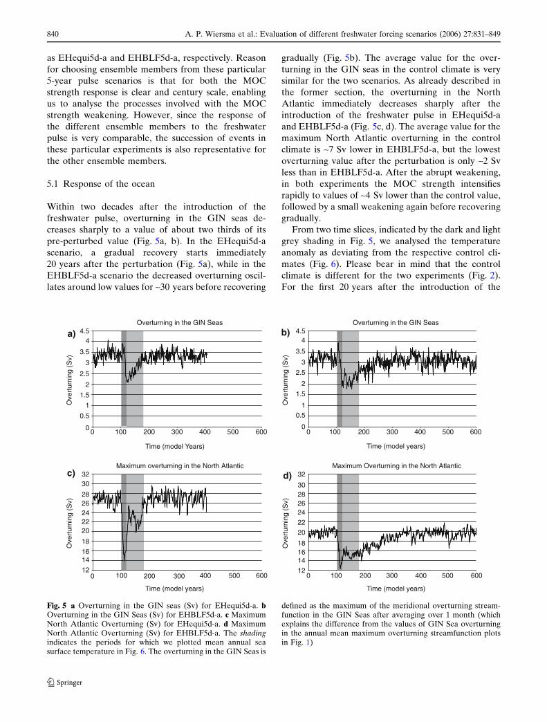
Within two decades after the introduction of the

freshwater pulse, overturning in the GIN seas de-

creases sharply to a value of about two thirds of its

pre-perturbed value (Fig. 5a, b). In the EHequi5d-a

scenario, a gradual recovery starts immediately

20 years after the perturbation (Fig. 5a), while in the

EHBLF5d-a scenario the decreased overturning oscil-

lates around low values for ~30 years before recovering

gradually (Fig. 5b). The average value for the over-

turning in the GIN seas in the control climate is very

similar for the two scenarios. As already described in

the former section, the overturning in the North

Atlantic immediately decreases sharply after the

introduction of the freshwater pulse in EHequi5d-a

and EHBLF5d-a (Fig. 5c, d). The average value for the

maximum North Atlantic overturning in the control

climate is ~7 Sv lower in EHBLF5d-a, but the lowest

overturning value after the perturbation is only ~2 Sv

less than in EHBLF5d-a. After the abrupt weakening,

in both experiments the MOC strength intensifies

rapidly to values of ~4 Sv lower than the control value,

followed by a small weakening again before recovering

gradually.

From two time slices, indicated by the dark and light

grey shading in Fig. 5, we analysed the temperature

anomaly as deviating from the respective control cli-

mates (Fig. 6). Please bear in mind that the control

climate is different for the two experiments (Fig. 2).

For the first 20 years after the introduction of the

Overturning in the GIN Seas

0

0.5

1

1.5

2

2.5

3

3.5

44.5

0 100 200 300 400 500 600

Time (model Years)

Ove

rtur

ning

(S

v)

Overturning in the GIN Seas

0

0.51

1.5

2

2.5

3

3.5

44.5

0 100 200 300 400 500 600

Time (model years)

Ove

rtur

ning

(S

v)

Maximum overturning in the North Atlantic

12

1416

18

2022242628

3032

0 100 200 300 400 500 600

Time (model years)

Ove

rtur

ning

(S

v)

Maximum Overturning in the North Atlantic

12

141618

20

22

24262830

32

0 100 200 300 400 500 600

Time (model years)

Ove

rtur

ning

(S

v)

a) b)

c) d)

Fig. 5 a Overturning in the GIN seas (Sv) for EHequi5d-a. bOverturning in the GIN Seas (Sv) for EHBLF5d-a. c MaximumNorth Atlantic Overturning (Sv) for EHequi5d-a. d MaximumNorth Atlantic Overturning (Sv) for EHBLF5d-a. The shadingindicates the periods for which we plotted mean annual seasurface temperature in Fig. 6. The overturning in the GIN Seas is

defined as the maximum of the meridional overturning stream-function in the GIN Seas after averaging over 1 month (whichexplains the difference from the values of GIN Sea overturningin the annual mean maximum overturning streamfunction plotsin Fig. 1)

840 A. P. Wiersma et al.: Evaluation of different freshwater forcing scenarios (2006) 27:831–849

123

freshwater pulse (dark shading in Fig. 5), clear differ-

ences exist between the two experiments. Both

experiments show a cooling belt from the north of

Scandinavia to Iceland that can be explained as a result

from reduced convection following the surface fresh-

ening (see Sect. 5.2). Surprisingly, in both scenarios, a

transient warm anomaly of more than 2�C is present

north of Iceland, coinciding with a northward retreat of

the ice cover there. This coincides with a shift in con-

vection in the GIN seas in the second decade after the

introduction of the freshwater towards a more south-

westerly position (not shown), and the subsequent

supply of heat to this site, through advection and from

the deep-sea to the surface. However, this shift almost

does not influence the overall GIN Sea overturning

strength (Fig. 5). Differences between the experiments

are a warm area south of Greenland in the EHBLF5d-

a experiment where in the EHequi5d-a experiment a

distinguished cooling is simulated. Again, an increase

in convection strength and associated ocean-to-atmo-

sphere heat flux is responsible for this warm anomaly,

which is so pronounced since convection was almost

absent in the control climate (Fig. 1c). Similarly, the

Labrador Sea shows a higher negative temperature

anomaly in the EHequi5d-a experiment. These differ-

ences show close agreement to the temperature

anomalies as observed between the EHequi and

EHBLF control climates (Fig. 2), and therefore can be

explained by the diminished deep-water formation in

the Labrador Sea and the Irminger Sea following the

freshwater pulse, which was already greatly diminished

in the EHBLF5d-a experiment as a response to the

constant adding of freshwater. Finally, a warming is

present off the east coast of America, which can be

explained by an intensification of the North Atlantic

subtropical gyre due to stronger winds during the

increasing of the meridional temperature gradient

occurring in the first 10 years after introduction of the

fresh water pulse. This may also explain the cooler

SSTs off Africa.

The SST anomaly for the two experiments during

years 20–80 after the introduction of the freshwater

pulse (light shading in Fig. 5) is similar, both in mag-

nitude and in spatial distribution (Fig. 6c, d). An

exception is the stronger cold anomaly at the southern

tip of Greenland in the EHequi5d-a experiment. In

both experiments, the main temperature decrease is

between Iceland and Greenland with a cooling up to

4�C, while the GIN Sea, Labrador Sea and the Atlantic

Ocean south of Greenland cool by around 1�C. The

extreme cooling in the Denmark Strait can be attrib-

uted to increased sea-ice cover here (not shown). The

other cooling sites appear to be less influenced by

increased sea-ice cover, and the cooling is caused by

reduced convection following the lowering of salinity

and subsequent decreased ocean-to-atmosphere heat-

flux at these sites.

These results support the idea that the introduction

of the baseline flow in the control climate mostly

influences the duration of the climate anomaly, and not

the magnitude. The difference in control climate, and

therefore the shutdown of LSW formation in the EH-

equi5d-a experiment relative to a control run with

LSW formation as opposed to the experiments without

baseline flow however, can explain most of the differ-

ences between the two experiments.

The 60-year mean SST anomalies of EHequi5d-a

and EHBLF5d-a in Fig. 6c, d shows a cooling around

the North Atlantic, which is consistent with the

spreading of proxy-evidence for the event (Alley et al.

2005; Rohling and Palike 2005; Wiersma and Renssen

2006). The magnitude of the cooling is smaller than

previously modelled (Renssen et al. 2001, 2002; Bauer

et al. 2004) and reaches less far south in Western

Europe and North America where, averaged over this

time period, the cooling does not exceed –0.5�C.

Therefore, in the present study, the mean annual

temperature averaged over a 60-year period (i.e.

between 20 and 80 years after the freshwater pulse) in

the EHequi5d-a and EHBLF5d-a scenarios under-

estimates the cooling as reconstructed from proxy-

evidence in Western Europe (Wiersma and Renssen

2006). The simulated cooling of ~1�C in northern

Scandinavia is smaller than simulated by Renssen et al.

(2001, 2002) and is more consistent with reconstructed

Northern Scandinavia summer temperatures that show

a decrease by up to 1�C (Korhola et al. 2000, 2002;

Seppa and Birks 2001). Therefore, the present model

appears to perform better for this crucial region in

ocean circulation. Simulated temperatures in this re-

gion are mainly controlled by oceanic heat flux to the

convection site near Spitzbergen. In model Version 2,

the Nordic Seas had a much stronger overturning than

in Version 3, imposing a stronger positive feedback and

therefore a too strong cooling (Renssen et al. 2001,

2002) when overturning is strongly reduced because of

the freshwater perturbation (more details about this

point are provided in Sect. 6). In terms of cooling in

central Greenland, most experiments show a shorter

cooling than the duration of the weakening of the

MOC, with a larger variability between the different

ensemble members. The scenarios without a baseline

flow that are perturbed by a freshwater pulse of,

respectively, 1.63 · 1014, 3.26 · 1014 and 4.89 · 1014 m3,

have an average duration of the cooling in Greenland

of respectively 50, 70 and 110 years with corresponding

A. P. Wiersma et al.: Evaluation of different freshwater forcing scenarios (2006) 27:831–849 841

123

maximum cooling of 4, 5 and 5�C. Similarly, the

scenarios with a baseline flow show an average dura-

tion of the cooling of 120, 190 and 260 years for these

respective scenarios with corresponding maximum

cooling of 4, 5 and 6�C. A recent study estimates the

duration of the cooling at ~160 years (Rasmussen

et al. 2006), with a magnitude of between 5.4 and

11.7�C (with best estimate of 7.4�C) (Leuenberger

et al. 1999) or 6 ± 2�C (Alley et al. 1997). Reasoning

backward, to simulate an event of ~160 years with a

magnitude that falls within these constraints, in our

model a freshwater pulse of between 1.63 · 1014 and

3.26 · 1014 m3 would have to be applied in the

EHBLF scenario.

5.2 Labrador Sea versus GIN Seas

A comparison of time-series of convection depth in the

Labrador Sea (Fig. 7, top figures) shows, as expected,

that convection depth for the control climate in EH-

equi5d-a is deeper than in the EHBLF5d-a scenario.

With the introduction of the freshwater pulse (at

t = 100), convection depth decreases dramatically fol-

lowing the decrease in sea surface salinity (Fig. 7a, c),

and recovers rapidly as the freshwater pulse stops.

Interestingly, after the freshwater pulse, convection

depth in the Labrador Sea in EHequi5d-a increases

markedly to values more than 200 m deeper than be-

fore the perturbation. The timing of the increase in

convection depth in the Labrador Sea coincides with

the fast removal of the salinity anomaly in the Labra-

dor Sea (Fig. 7a, b) and the fast acceleration of MOC

in EHequi5d-a and, although smaller in magnitude,

EHBLF5d-a (Fig. 5c, d).

The increase in convection depth is probably caused

by the interaction between temperature and salinity in

the density of the surface waters of the Labrador Sea.

With the introduction of the freshwater pulse, sea

surface density rapidly decreases in both scenarios

(Fig. 8a, b), until the decrease slows down for around a

decade as the scenarios come close to minimum values

of ~1,026.4 kg/m3 in EHequi5d-a and ~1,025.8 kg/m3 in

EHBLF5d-a. From this point on, the two scenarios

show a different path. In EHequi5d-a the density

0-0.5-1-1.5-2-2.5-3-3.5

80N

60N

40N

20N

EQ80W 60W 40W 20W 0 20E 40E

0-0.5-1-1.5-2-2.5-3-3.5

0.5

-4

80N

60N

40N

20N

EQ80W 60W 40W 20W 0 20E 40E

80N

60N

40N

20N

EQ80W 60W 40W 20W 0 20E 40E

80N

60N

40N

20N

EQ80W 60W 40W 20W 0 20E 40E

0-0.5-1-1.5

0.5

1.52

1

0-0.5-1-1.5

0.5

1.52

1

a) b)

c) d)

Tem

perature (°C)

Tem

perature (°C)

Tem

perature (°C)

Tem

perature (°C)

Fig. 6 Maps showing mean annual SST anomalies (�C) asdeviating from the control climate for a EHequi5d-a and bEHBLF5d-a for the first 20 years after the introduction of thefreshwater pulse, and c EHequi5d-a and d EHBLF5d-a for the

years 20–80 after the introduction of the freshwater pulse. Theperiods used are indicated in Fig. 5 as dark shading for the first20 years, and light shading for the years 20–80

842 A. P. Wiersma et al.: Evaluation of different freshwater forcing scenarios (2006) 27:831–849

123

rapidly increases as salinity increases, but the temper-

atures are lower than in the decreasing density trajec-

tory. At t = 120 the increase in density slows down and

SST becomes colder until t = 130. This period with

colder SSTs corresponds to the period with deeper

convection in Fig. 7a. From this point on, temperatures

0

100

200

300

400

500

600

700

0

200

400

600

800

1000

1200

1400

0

1

2

3

4

5

6

32

33

34

35

0

1

2

3

4

3434.234.434.634.83535.235.4

0

100

200

300

400

500

600

700

32

33

34

35

0 100 200 300 4000 100 200 300 400

0 100 200 300 4000

1

2

3

4

5

6

0 100 200 300 400

0

1

2

3

4

0

200

400

600

800

1000

1200

1400

3434.234.434.634.83535.235.4

0 100 200 300 400

0 100 200 300 400

0 100 200 300 400

0 100 200 300 400

Con

vect

ion

dept

h (m

)

Time (model years)Time (model years)

Con

vect

ion

dept

h (m

)C

onve

ctio

n de

pth

(m)

Con

vect

ion

dept

h (m

)S

alinity (psu)S

alinity (psu)

Salinity (psu)

Salinity (psu)

Tem

pera

ture

(°C

)Te

mpe

ratu

re (

°C)

Tem

pera

ture

(°C

)Te

mpe

ratu

re (

°C)

EHBLF5d-aEHequi5d-a

Labrador Sea

GIN SeaTime (model years) Time (model years)

Time (model years) Time (model years)

Time (model years)Time (model years)EHBLF5d-aEHequi5d-a

a) b)

c) d)

Fig. 7 Twenty-one-year running mean time series of Februaryconvection depth (m) (grey shading), February sea surfacesalinity (psu) and February sea surface temperature (�C) in thepredominant convection area in the Labrador Sea (between 60

and 50�W and 57 and 63�N, upper figures) and the GIN Sea(between 5 and 15�E and 73 and 77�N, lower figures) forEHequi5d-a (a, c) and EHBLF5d-a (b, d)

A. P. Wiersma et al.: Evaluation of different freshwater forcing scenarios (2006) 27:831–849 843

123

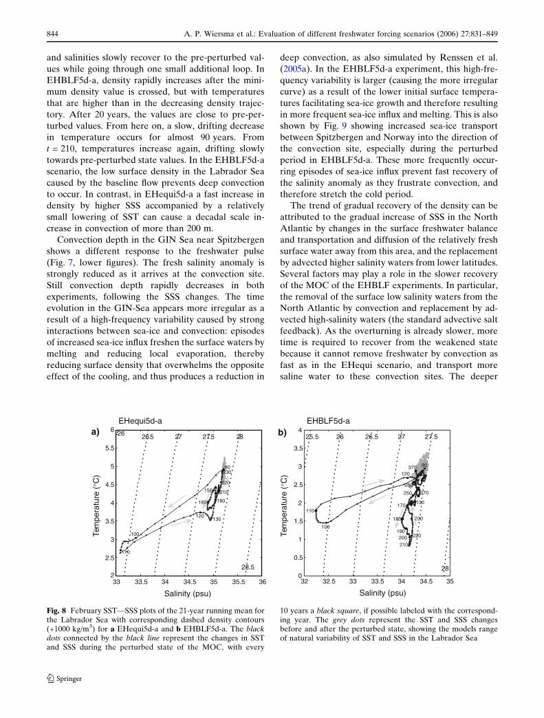
and salinities slowly recover to the pre-perturbed val-

ues while going through one small additional loop. In

EHBLF5d-a, density rapidly increases after the mini-

mum density value is crossed, but with temperatures

that are higher than in the decreasing density trajec-

tory. After 20 years, the values are close to pre-per-

turbed values. From here on, a slow, drifting decrease

in temperature occurs for almost 90 years. From

t = 210, temperatures increase again, drifting slowly

towards pre-perturbed state values. In the EHBLF5d-a

scenario, the low surface density in the Labrador Sea

caused by the baseline flow prevents deep convection

to occur. In contrast, in EHequi5d-a a fast increase in

density by higher SSS accompanied by a relatively

small lowering of SST can cause a decadal scale in-

crease in convection of more than 200 m.

Convection depth in the GIN Sea near Spitzbergen

shows a different response to the freshwater pulse

(Fig. 7, lower figures). The fresh salinity anomaly is

strongly reduced as it arrives at the convection site.

Still convection depth rapidly decreases in both

experiments, following the SSS changes. The time

evolution in the GIN-Sea appears more irregular as a

result of a high-frequency variability caused by strong

interactions between sea-ice and convection: episodes

of increased sea-ice influx freshen the surface waters by

melting and reducing local evaporation, thereby

reducing surface density that overwhelms the opposite

effect of the cooling, and thus produces a reduction in

deep convection, as also simulated by Renssen et al.

(2005a). In the EHBLF5d-a experiment, this high-fre-

quency variability is larger (causing the more irregular

curve) as a result of the lower initial surface tempera-

tures facilitating sea-ice growth and therefore resulting

in more frequent sea-ice influx and melting. This is also

shown by Fig. 9 showing increased sea-ice transport

between Spitzbergen and Norway into the direction of

the convection site, especially during the perturbed

period in EHBLF5d-a. These more frequently occur-

ring episodes of sea-ice influx prevent fast recovery of

the salinity anomaly as they frustrate convection, and

therefore stretch the cold period.

The trend of gradual recovery of the density can be

attributed to the gradual increase of SSS in the North

Atlantic by changes in the surface freshwater balance

and transportation and diffusion of the relatively fresh

surface water away from this area, and the replacement

by advected higher salinity waters from lower latitudes.

Several factors may play a role in the slower recovery

of the MOC of the EHBLF experiments. In particular,

the removal of the surface low salinity waters from the

North Atlantic by convection and replacement by ad-

vected high-salinity waters (the standard advective salt

feedback). As the overturning is already slower, more

time is required to recover from the weakened state

because it cannot remove freshwater by convection as

fast as in the EHequi scenario, and transport more

saline water to these convection sites. The deeper

EHequi5d-a

Tem

pera

ture

(°C

)

Tem

pera

ture

(°C

)

Salinity (psu)

6

5.5

5

4.5

4

3.5

3

2.5

233 33.5 34 34.5 35 35.5 36

26 26.5 27 27.5 28

28.5

EHBLF5d-a

Salinity (psu)

1.5

1

0.5

0

2

2.5

3

3.5

4

32 32.5 33 33.5 34 34.5 35

25.5 26 26.5 27 27.5

28

a) b)

90

100

110

120

130170

180

190200210

220

230

250 270

280

37090

120130

150

160 180

210

220

100

110

230

Fig. 8 February SST—SSS plots of the 21-year running mean forthe Labrador Sea with corresponding dashed density contours(+1000 kg/m3) for a EHequi5d-a and b EHBLF5d-a. The blackdots connected by the black line represent the changes in SSTand SSS during the perturbed state of the MOC, with every

10 years a black square, if possible labeled with the correspond-ing year. The grey dots represent the SST and SSS changesbefore and after the perturbed state, showing the models rangeof natural variability of SST and SSS in the Labrador Sea

844 A. P. Wiersma et al.: Evaluation of different freshwater forcing scenarios (2006) 27:831–849

123

convection in the Labrador Sea in response to the

freshwater pulse in the EHequi scenario may be

especially efficient in recovering salinity in the North

Atlantic, as relatively fresh water is removed with in-

creased LSW production, and more saline surface

waters are advected to the north. Since this convection

in the Labrador Sea is suppressed by the constant

baseline flow, MOC recovery takes longer in the

EHBLF scenario. This hypothesis is consistent with the

coincidence in EHequi5d-a of the increase in convec-

tion depth in the Labrador Sea, the fast removal of the

salinity anomaly there and the fast acceleration of the

MOC strength.

The lower temperatures in the control climate of

EHBLF and during the MOC slowdown in the GIN

Sea may also play a role. The lower temperatures

facilitate sea-ice growth and therefore cause an in-

creased chance of sea ice influx at these sites, which

prevents convection to occur by the freshening of

surface waters and therefore slows down the removal

of the salinity anomaly.

In summary, Labrador Sea convection and GIN Sea

convection show a different response to the freshwater

pulse: both show a decrease in convection depth, but in

the Labrador Sea this general decrease is interrupted

by a decadal scale increase in EHequi5d-a. In the

EHBLF5d-a experiment, the lower surface water

density in the Labrador Sea caused by the baseline flow

dampens this convection depth increase and in the

GIN Seas the slowdown is prolonged due to lower

temperatures and more sea-ice interactions. In the

Labrador Sea, such a delicate balance between SSS and

SST in controlling deep convection has already been

observed on longer time scales in proxy-data (Solignac

et al. 2004) and in a transient Holocene climate simu-

lation under greenhouse gas and astronomical forcing

(Renssen et al. 2005a).

6 Comparison with other model studies

Our study is comparable to previous modelling stud-

ies on the 8.2 ka BP event by Renssen et al. (2001,

2002) and Bauer et al. (2004). Renssen et al. (2001,

2002) experimented with a constant volume of

4.67 · 1014 m3 freshwater that was released with dif-

fering durations (10, 20, 50 and 500 years) into the

Labrador Sea. These experiments were performed

with the previous version of the ECBilt-CLIO climate

model that had no representation of LSW formation

and a less realistic GIN Seas overturning value. Fur-

thermore the released volume of 4.67 · 1014 m3 ex-

ceeds the highest estimate found in the literature

(Tornqvist et al. 2004). In these experiments, the

model’s MOC shifted to a new unstable state, making

the recovery unpredictable as it was governed by

high-frequency variability involving the atmosphere.

Still, the climate response to the freshwater pulse of

one of the 20 years pulse duration experiments

did show a good agreement with proxy-evidence

(Wiersma and Renssen 2006). In the experiments

performed in this study with the ECBilt-CLIO-

VECODE Version 3, we found no indication for such

an unstable state with the freshwater pulses that were

applied. Therefore, in the current experiments high-

frequency variability is of minor influence on the

duration of the event. In the Renssen et al. (2002)

paper, the existence of the unstable state is prolonged

by a strong positive feedback by enhanced sea-ice

export from the Barents Sea, representing a consid-

erable increase in freshwater transport to the site of

convection. In our model we do see enhanced export

from the Barents Sea to the site of convection, as

described in Sect. 5.2, but to a much lesser extent.

This weaker positive feedback in combination with a

smaller share of the GIN Sea overturning (17 Sv vs.

Fig. 9 Twenty-one-year running mean (black line) and annualmean (grey line) of the sea-ice transport (Sv) between Spitzber-gen and Norway, a for EHequi5d-a and b for EHBLF5d-a.

Negative values indicate a predominant transport in westwarddirection (i.e. towards GIN seas convection site)

A. P. Wiersma et al.: Evaluation of different freshwater forcing scenarios (2006) 27:831–849 845

123

3 Sv) in the total North Atlantic overturning may be

the reason that such an unstable state is not present in

the current experiments, which makes the MOC

recovery more predictable.

Bauer et al. (2004) released a volume of

1.6 · 1014 m3 freshwater into the North Atlantic

Ocean between 50 and 70�N in an early Holocene

climate. In their experiments with the CLIMBER-2

model, a freshwater baseline flow caused an increased

chance of a longer collapse of the MOC to freshwater

perturbations. Also in these experiments, the MOC

shifted into an unstable climate state, which made the

duration of the perturbed state unpredictable. Unfor-

tunately, the CLIMBER-2 model has a coarse spatial

resolution, and the ocean basin variables are computed

as zonal means for the oceans, making a study on the

respective roles of convection in the Labrador Sea and

GIN Seas impossible.

The current study suggests that the magnitude and

duration of the weakening in overturning circulation

is mainly a function of the volume of freshwater re-

leased, at least for the scenarios tested here. A sim-

ilar gradual recovery after a freshwater perturbation

was found by Manabe and Stouffer (1995) in an

attempt to simulate the Younger Dryas cooling. If

these findings are realistic, it means that from

knowing the exact volume of freshwater that was

released during the lake outburst, new information

on the sensitivity to perturbations of the early

Holocene climate state can be derived. This would

also provide a strong constraint on models and on

their representation of the response of the MOC to

freshwater release. Unfortunately, the uncertainty on

this volume is presently still large, implying that it is

possible to find a realistic scenario that reproduces

the observed event reasonably well for different

model sensitivities.

In our simulations, the presence of a baseline flow

from the melting LIS is of great influence on the

response of the MOC. This implies that the use of

the 8.2 ka BP event in the Paleoclimate-hosing

Model Intercomparison Project (PhMIP, Schlessinger

2005) to assess the performance of models is more

complex than introducing a short freshwater pulse,

and the influence of a baseline flow from the melting

LIS should be tested in the models. Furthermore our

results show that the Labrador Sea is an important

and sensitive player in the global ocean circulation.

Other investigators have already suggested that the

current freshening in combination with greenhouse

warming may well promote the collapse of the LSW

formation (Wood et al. 1999; Weaver and Hillaire-

Marcel 2004).

7 Summary and conclusions

In this paper we showed the results of freshwater

perturbation experiments focused on the early Holo-

cene (8.5 ka BP) climate. First we experimented with

the introduction of a realistic baseline flow from the

LIS and compared this with proxy data. In this way we

obtained two early Holocene reference climate states.

Next, to simulate the 8.2 ka BP event, we perturbed

these two early Holocene climate states with freshwa-

ter pulses varying in volume and duration into the

Labrador Sea based on recent estimates constrained by

geological evidence. We investigated the response of

the MOC and the response of the ocean. From these

experiments, we come to the following conclusions:

(1) The simulated early Holocene climate with a

baseline flow from the LIS results in ceased con-

vection in the Labrador Sea, and a cold anomaly

of ~2�C around the Labrador Sea gradually

decreasing to ~1�C in the Irminger Sea, compared

to a simulation without a baseline flow. These

results are consistent with proxy-data that record

absence of LSW formation in the early Holocene.

(2) In all experiments, the MOC intensity weakens

sharply, followed by a gradual recovery to pre-

perturbed values.

(3) In our experiments, the volume of the freshwater

pulse is the dominant factor in the response of the

MOC. Duration and timing of the freshwater

pulse have almost no effect on the response of the

MOC, at least for the relatively short release

durations (i.e. 1, 2 and 5 years) that are tested

here. This outcome suggests that future research

should focus on better estimates on the volume of

freshwater that was released. Sea level recon-

structions as performed by Tornqvist et al. (2004)

provide these estimates as they include the

amount of ice that was released together with the

freshwater.

(4) The experiments with a baseline flow into the

Labrador Sea show a slower recovery of the MOC

strength. Therefore, in an early Holocene climate

with a baseline flow, less freshwater is needed to

produce an event of similar duration than without

a baseline flow. This implies that model inter-

comparison studies covering the 8.2 ka BP event

should consider including a representation of a

baseline flow in their early Holocene climate

state.

(5) By introducing a volume of 1.63 · 1014 m3, the

estimated volume of the Laurentide lakes

(Leverington et al. 2002), the maximum simulated

846 A. P. Wiersma et al.: Evaluation of different freshwater forcing scenarios (2006) 27:831–849

123

duration of the weakening of the MOC strength is

~160 years. In the experiments without a baseline

flow, this volume produces a weakening of only

~100 years. To produce an event in Greenland

with a duration of ~160 years and a magnitude,

i.e. within the constraints of proxy evidence, in

our model, a freshwater pulse of between

1.63 · 1014 and 3.26 · 1014 m3 would have to be

applied in the EHBLF control climate.

(6) In contrast with other modelling studies, no

indication is found for an intermediate stable

weakened state of the MOC in our model with

the freshwater volumes and release durations

used in these experiments.

(7) Convection in the Labrador Sea intensifies peri-

odically during the perturbed state of the MOC.

In the experiments with a baseline flow this is

dampened by the lower density of the surface

water, but still present. Since LSW is relatively

fresh, this intensification may play a role in the

faster recovery of the MOC in experiments

without a baseline flow.

References

Alley RB, Mayewski PA, Sowers T, Stuiver M, Taylor KC, ClarkPU (1997) Holocene climatic instability—a prominent,widespread event 8200 yr ago. Geology 25:483–486

Alley RB, Agustsdottir AM (2005) The 8k event: cause andconsequences of a major Holocene abrupt climate change.Quaternary Sci Rev 24:1123–1149

Barber DC, Dyke A, Hillaire-Marcel C, Jennings AE, AndrewsJT, Kerwin MW, Bilodeau G, McNeely R, Southon J,Morehead MD, Gagnon J-M (1999) Forcing of the coldevent of 8,200 years ago by catastrophic drainage of lau-rentide lakes. Nature 400:344–348

Bauer E, Ganopolski A, Montoya M (2004) Simulation of thecold climate event 8200 years ago by meltwater outburstfrom Lake Agassiz. Paleoceanography 19:PA3014. DOI10.1029/2004PA001030

Berger A, Loutre MF (1991) Insolation values for the climate ofthe last 10 million years. Quaternary Sci Rev 10:297–317

Berger A (1992) Orbital variations and insolation database.IGBP PAGES/World Data Center-A for PaleoclimatologyData Contribution Series # 92-007. NOAA/NGDC Paleo-climatology Program, Boulder, CO, USA

Bond GC, Kromer B, Beer J, Muscheler R, Evans MN, ShowersW, Hoffmann S, Lotti-Bond R, Hajdas I, Bonani G (2001)Persistent solar influence on north atlantic climate duringthe holocene. Science 294:2130–2133

Brovkin V, Bendtsen J, Claussen M, Ganopolski A, Kubatzki C,Petoukhov V, Andreev A (2002) Carbon cycle, vegetation,and climate dynamics in the Holocene: experiments with theCLIMBER-2 model. Global Biogeochem Cycles 16(4):1139.DOI 10.1029/2001GB001662

Campin J-M, Goosse H (1999) Parameterization of density-driven downsloping flow for a coarse-resolution oceaanmodel in z-coordinate. Tellus 51A:412–430

Clarke GKC, Leverington DW, Teller JT, Dyke AS (2004)Paleohydraulics of the last outburst flood from glacial lakeagassiz and the 8200 BP cold event. Quaternary Sci Rev23:389–407

Clarke GKC, Leverington DW, Teller JT, Dyke AS, Marshall SJ(2005) Fresh arguments against the shaw megafloodhypothesis. A reply to comments by David Sharpe on pa-leohydraulics of the last outburst flood from glacial lakeagassiz and the 8200 BP cold event. Quaternary Sci Rev24:1533–1541

Cottet-Puinel M, Weaver AJ, Hillaire-Marcel C, de Vernal A,Clark PU, Eby M (2004) Variation of labrador sea deepwater formation over the last glacial cycle in a climatemodel of intermediate complexity. Quaternary Sci Rev23:449–465

Cubasch U, Meehl GA, Boer GJ, Stouffer RJ, Dix M, Noda A,Senior CA, Raper S, Yap KS (2001) Projections of futureclimate change. in climate change 2001. In: Houghton JT,Ding Y, Griggs DJ, Noguer M, van der Linden PJ, Dai X,Maskell K, Johnson CA (eds) The scientific basis. contri-bution of working group I to the third assessment report ofthe intergovernmental panel on climate change. CambridgeUniversity Press, New York, pp 525–582

Deleersnijder E, Campin J-M (1995) On the computation of thebarotropic mode of a free-surface world ocean model. AnnGeophys 13:675–688

Dyke AS, Prest VK (1989) Paleogeographie de l’amerique dunord septentrionale, entre 18 000 and 5000 ans avant lepresent. Commission geologique du Canada carte, echelle,1703A, 1/12500000

Dyke AS (2003) An outline of north american deglaciation withemphasis on central and northern Canada. In: Ehlers J (ed)Extent and chronology of quaternary glaciation. Elsevier,Amsterdam, pp 371–406

Elliot M, Labeyrie L, Duplessy J-C (2002) Changes in NorthAtlantic deep-water formation associated with the dansg-aard-oeschger temperature oscillations (60-10 ka). Quater-nary Sci Rev 21:1153–1165

Fichefet T, Morales Maqueda MA (1997) Sensitivity of a globalsea ice model to the treatment of ice thermodynamics anddynamics. J Geophys Res 102:609–646

Gent JR, McWilliams JC (1990) Isopycnal mixing in oceangeneral circulation models. J Phys Oceanogr 20:150–155

Goosse H, Fichefet T (1999) Importance of ice-ocean interac-tions for the global ocean circulation: a model study.J Geophys Res 104:23337–23355

Goosse H, Deleersnijder E, Fichefet T, England MH (1999)Sensitivity of a global coupled ocean-sea ice model to theparameterization of vertical mixing. J Geophys Res104(C6):13681–13695

Goosse H, Renssen H (2001) On the delayed response of sea icein the Southern Ocean to an increase in greenhouse gasconcentrations. Geophys Res Lett 28:3469–3473

Goosse H, Selten FM, Haarsma RJ, Opsteegh JD (2001) Dec-adal variability in high northern latitudes as simulated by anintermediate-complexity climate model. Ann Glaciol33:525–532

Goosse H, Selten FM, Haarsma RJ, Opsteegh JD (2002) Amechanism of decadal variability of the sea-ice volume inthe Northern Hemisphere. Clim Dynam 19:61–83. DOI10.1007/s00382-00001-00209-00385

A. P. Wiersma et al.: Evaluation of different freshwater forcing scenarios (2006) 27:831–849 847

123

Goosse H, Selten FM, Haarsma RJ, Opsteegh JD (2003) Largesea-ice volume anomalies simulated in a coupled climatemodel. Clim Dynam 20:523–536. DOI 510.1007/s00382-00002-00290-00384

Goosse H, Renssen H, Timmermann A, Bradley RS (2005)Internal and forced climate variability during the last mil-lennium: a model-data comparison using ensemble simula-tions. Quaternary Sci Rev 24(12–13):1345–1360

von Grafenstein U, Erlenkeuser H, Muller J, Jouzel J, Johnsen S(1998) The cold event 8200 years ago documented in oxygenisotope records of precipitation in Europe and Greenland.Clim Dynam 14:73–81

Hillaire-Marcel C, de Vernal A, Bilodeau G, Weaver AJ (2001)Absence of deep-water formation in the Labrador Seaduring the last interglacial period. Nature 410:1073–1077

Josenhans HW, Zevenhuizen J (1990) Dynamics of the lauren-tide ice sheet in Hudson Bay, Canada. Mar Geol 92:1–26

Keigwin LD, Lehman SJ (1994) Deep circulation change linkedto heinrich event 1 and younger dryas in a middepth NorthAtlantic core. Paleoceanography 9(2):185–194

Klitgaard-Kristensen D, Sejrup HP, Haflidason H, Johnsen S,Spurk M (1998) A regional 8200 cal. yr BP cooling event innorthwest Europe, induced by final stages of the laurentideice-sheet deglaciation? J Quaternary Sci 13:165–169

Knutti R, Fluckinger J, Stocker TF, Timmermann A (2004) Stronghemispheric coupling of glacial climate through freshwaterdischarge and ocean circulation. Nature 430:851–856

Korhola A, Weckstrom J, Holmstrom L, Erasto P (2000) Aquantitative holocene climatic record from diatoms innorthern fennoscandia. Quaternary Res 54:284–294

Korhola A, Vasko K, Toivonen HTT, Olander H (2002) Holo-cene temperature changes in northern fennoscandia recon-structed from chironomids using Bayesian modelling.Quaternary Sci Rev 21:1841–1860

Leuenberger MC, Lang C, Schwander J (1999) Delta15N mea-surements as a calibration tool for the paleothermometerand gas-ice age differences: a case study for the 8200 BPevent in GRIP ice. J Geophys Res 104(18):22163–22170

Leverington D, Mann JD, Teller JT (2002) Changes inbathymetry and volume of glacial lake agassiz between 9200and 7700 14C yr BP. Quaternary Res 57:244–252. DOI 210-1006/qres-2001-2311

Licciardi JM, Teller JT, Clark PU (1999) Freshwater routing ofthe laurentide ice sheet during the last deglaciation. In:Clark PU, Webb RS, Keigwin LD (eds) Mechanisms ofGlobal climate change at millennial time scales. AmericanGeophysical Union, Washington, DC. Geophys Monogr112:177–201

Manabe S, Stouffer RJ (1995) Simulation of abrupt climatechange induced by freshwater input to the North AtlanticOcean. Nature 378:165–167

Manabe S, Stouffer RJ (1997) Coupled ocean-atmosphere modelresponse to freshwater input: comparison to younger dryasevent. Paleoceanography 12:321–336

Mellor GL, Yamada T (1982) Development of a turbulenceclosure model for geophysical fluid problems. Rev GeophysSpace Phys 20:851–875

Moros M, Emeis K, Risebrobakken B, Snowball I, Kuijpers A,McManus J, Jansen E (2004) Sea surface temperatures andice rafting in the Holocene North Atlantic: climate influ-ences on northern Europe and Greenland. Quaternary SciRev 23:2113–2126

Opsteegh JD, Haarsma RJ, Selten FM, Kattenberg A (1998)ECBILT: a dynamic alternative to mixed boundary condi-tions in ocean models. Tellus 50A:348–367

Peltier WR (1994) Ice age paleotopography. Science 265:195–201Rasmussen SO, Andersen KK, Svensson AM, Steffensen JP,

Vinther BM, Clausen HB, Siggaard-Andersen M-L, JohnsenSJ, Larsen LB, Dahl-Jensen D, Bigler M, Rothlisberger R,Fischer H, Goto-Azuma K, Hansson ME, Ruth U (2006) Anew Greenland ice core chronology for the last glacialtermination. J Geophys Res 111:D06102. DOI 10.1029/2005JD006079

Raynaud D, Barnola J-M, Chappellaz J, Blunier T, IndermuhleA, Stauffer B (2000) The ice record of Greenhouse gases: aview in the context of future changes. Quaternary Sci Rev19:9–17

Renssen H, Goosse H, Fichefet T, Campin J-M (2001) The 8.2kyr BP event simulated by a global atmosphere–sea-ice–ocean model. Geophys Res Lett 28:1567–1570

Renssen H, Goosse H, Fichefet T (2002) Modeling the effect offreshwater pulses on the early Holocene climate: the influ-ence of high frequency climate variability. Paleoceanogra-phy 17:1020. DOI 1010.1029/2001PA000649

Renssen H, Goosse H, Fichefet T (2005a) Contrasting trends inNorth Atlantic deep-water formation in the labrador seaand nordic seas during the holocene. Geophys Res Lett32:L08711. DOI 08710.01029/02005GL022462

Renssen H, Goosse H, Fichefet T, Brovkin V, Driesschaert E,Wolk F (2005b) Simulating the holocene climate evolutionat northern high latitudes using a coupled atmosphere-seaice-ocean-vegetation model. Clim Dynam 24(1):23–43

Rohling EJ, Palike H (2005) Centennial-scale climate coolingwith a sudden cold event around 8,200 years ago. Nature434:975–979

Rossow WB, Walker AW, Beuschel DE, Roiter MD (1996)International satellite cloud climatology project (ISCCP)documentation of new cloud datasets. World Meteorologi-cal Organisation, Geneva, WMO/TD-No 737

Schaeffer M, Selten FM, Opsteegh JD, Goosse H (2002) Intrinsiclimits to predictability of abrupt regional climate change inIPCC SRES scenarios. Geophys Res Lett 29(16):1767. DOI10.1029/2002GL015254

Schlessinger M (2005) Proposal for PMIP2/1ACE Paleo-hosingModel Intercomparison Project (PhMIP). WUN-ACE Kick-Off Meeting 15th–18th May 2005 (Abstracts)

Seppa H, Birks HJB (2001) July mean temperature and annualprecipitation trends during the holocene in the fennoscan-dian tree-line area: pollen-based climate reconstructions.Holocene 11:527–539

Sharpe D (2005) Comments on: paleohydraulics of the last out-burst flood from glacial lake agassiz and the 8200 BP coldevent by Clarke et al [Quaternary Sci Rev 23(2004):389–407]. Quaternary Sci Rev 24:1529–1532

Solignac S, de Vernal A, Hillaire-Marcel C (2004) Holocene sea-surface conditions in the North Atlantic—contrasted trendsand regimes in the western and eastern sectors (LabradorSea vs. Iceland Basin). Quaternary Sci Rev 23:319–334

Stocker TF, Wright DG (1991) Rapid transitions of the ocean’sdeep circulation induced by changes in surface water fluxes.Nature 351:729–732

Teller JT, Leverington DW, Mann JD (2002) Freshwater out-bursts to the oceans from glacial Lake Agassiz and their rolein climate change during the last deglaciation. QuaternarySci Rev 21:879–887

Tornqvist TE, Bick SJ, Gonzalez JL, van der Borg K, de JongAFM (2004) Tracking the sea-level signature of the 8.2 kacooling event: new constraints from the mississippi delta.Geophys Res Lett 31:L23309. DOI 23310.21029/22004GL021429

848 A. P. Wiersma et al.: Evaluation of different freshwater forcing scenarios (2006) 27:831–849

123

Upham W (1896) The glacial lake agassiz. Monographs of theUnited States geological survey, vol. 25. Washington Gov-ernment Printing Office, Washington

Veillette JJ (1994) Evolution and paleohydrology of glacial lakesBarlow and Ojibway. Quaternary Sci Rev 13:945–971

Vellinga M, Wood RA (2002) Global climatic impacts of a col-lapse of the Atlantic thermohaline circulation. Clim Change54:251–267

de Vernal (1997) Researchers look for links among paleoclimateevents. Eos 78:247–249

Weaver AJ, Hillaire-Marcel C (2004) Global warming and thenext ice age. Science 304:400–402

Wiersma AP, Renssen H (2006) Model-data comparison for the8.2 ka BP event: confirmation of a forcing mechanism bycatastrophic drainage of laurentide lakes. Quaternary SciRev 25:63–88

Wood RA, Keen AB, Mitchell JFB, Gregory JM (1999)Changing spatial structure of the thermohaline circulation inresponse to atmospheric CO2 forcing in a climate model.Nature 399:572–575

A. P. Wiersma et al.: Evaluation of different freshwater forcing scenarios (2006) 27:831–849 849

123