Anthropogenic climate change for 1860 to 2100 simulated with the HadCM3 model under updated...

Anthropogenic climate change for 1860 to 2100 simulatedwith the HadCM3 model under updated emissions scenarios

Received: 29 April 2002 / Accepted: 31 October 2002 / Published online: 18 February 2003� Springer-Verlag 2003

Abstract In this study we examine the anthropogenicallyforced climate response over the historical period, 1860to present, and projected response to 2100, usingupdated emissions scenarios and an improved coupledmodel (HadCM3) that does not use flux adjustments.We concentrate on four new Special Report on EmissionScenarios (SRES) namely (A1FI, A2, B2, B1) preparedfor the Intergovernmental Panel on Climate ChangeThird Assessment Report, considered more self-consis-tent in their socio-economic and emissions structure,and therefore more policy relevant, than older scenarioslike IS92a. We include an interactive model representa-tion of the anthropogenic sulfur cycle and both directand indirect forcings from sulfate aerosols, but omit thesecond indirect forcing effect through cloud lifetimes.The modelled first indirect forcing effect through clouddroplet size is near the centre of the IPCC uncertaintyrange. We also model variations in tropospheric andstratospheric ozone. Greenhouse gas-forced climatechange response in B2 resembles patterns in IS92a but issmaller. Sulfate aerosol and ozone forcing substantiallymodulates the response, cooling the land, particularlynorthern mid-latitudes, and altering the monsoonstructure. By 2100, global mean warming in SRES sce-narios ranges from 2.6 to 5.3 K above 1900 and pre-cipitation rises by 1%/K through the twenty first century(1.4%/K omitting aerosol changes). Large-scale patternsof response broadly resemble those in an earlier model(HadCM2), but with important regional differences,particularly in the tropics. Some divergence in futureresponse occurs across scenarios for the regions

considered, but marked drying in the mid-USA andsouthern Europe and significantly wetter conditions forSouth Asia, in June–July–August, are robust and sig-nificant.

1 Introduction

There is growing expectation that increases in the con-centrations of greenhouse gases arising from human ac-tivity will lead to substantial changes in climate in thetwenty first century. Indeed, there is already evidencethat anthropogenic emissions of greenhouse gases(GHGs) have altered the large-scale patterns of tem-perature over the twentieth century (Santer et al. 1996;Tett et al. 1999; Barnett et al. 1999; Stott et al. 2001;Mitchell et al. 2001), although natural factors, includingchanges in solar output and episodic volcanic emissions,may also have contributed. Future climate change willprobably be dominated by the response to anthropogenicforcing factors. Large uncertainties remain, however, inthe expected anthropogenic climate response, partlythrough model uncertainty in the projected climate sen-sitivity to increasing GHGs and partly as a result of bothphysical and modelling uncertainties in the amplitudeand geographical patterns of non-GHG forcings whichmodulate this GHG-forced response (particularly fromsulfate aerosol indirect cooling effects).

The main motivation for the present study is toprovide up-to-date estimates of global climate changesuitable for deriving impacts assessments on regionalscales with self-consistent scenario assumptions. Eventhough some of the regional details may be unreliable,this approach at least gives a picture of possible conse-quences of alternative future emissions scenarios, de-rived in a physically consistent way, which can beinterpreted for policymakers in the context of negotia-tions to limit emissions so as to prevent ’dangerous’climate change.

Climate Dynamics (2003) 20: 583–612DOI 10.1007/s00382-002-0296-y

T.C. Johns Æ J.M. Gregory Æ W.J. Ingram

C.E. Johnson Æ A. Jones Æ J.A. LoweJ.F.B. Mitchell Æ D.L. Roberts Æ D.M.H. Sexton

D.S. Stevenson Æ S.F.B. Tett Æ M.J. Woodage

T.C. Johns (&) Æ J.M. Gregory Æ W.J. Ingram Æ C.E. JohnsonA. Jones Æ J.A. Lowe Æ J.F.B. Mitchell Æ D.L. RobertsD.M.H. Sexton Æ S.F.B. Tett Æ M.J. WoodageMet Office, Hadley Centre for Climate Prediction and Research,London Road, Bracknell, RG12 2SY, UKE-mail: [email protected]

D.S. StevensonDepartment of Meteorology, University of Edinburgh King’sBuildings, Edinburgh EH9 3JZ, Scotland, UK,

Some questions that arise are whether GHG-inducedwarming (determined by global average emissions) willdominate, or whether local sulfate aerosol forcing (muchmore dependent on local emissions) will be a significantfactor over the twenty first century and, if the latter,what differences in the regional responses might be ex-pected under different emissions scenarios? Could non-linear climate-chemistry feedbacks become increasinglyimportant to consider in future, with an implication ofadded importance attached to the details of alternativeemissions pathways that result in similar time-integratedemissions? To tackle such questions it is important thatthere should be consistency and some plausibility aboutthe emissions scenarios used to force climate models.The IPCC SRES (‘Special Report on Emissions Sce-narios’, Nakicenovic et al. 2000) marker scenarios de-veloped in conjunction with the IPCC Third AssessmentReport, have been developed specifically to providemore self-consistent and up-to-date scenarios for climatemodelling than hitherto. We have therefore primarilyadopted these in the present study, though we also referback to the older IS92a scenario which has already beenused extensively in climate impact studies (e.g. USNational Assessment Report 2000; Hulme et al. 1999;Hulme and Jenkins 1998).

Given emission scenarios of GHGs, sulfur and otheranthropogenic precursor gases, understanding the cli-mate sensitivity to the resulting anthropogenic forcingsand the interactions between climate change, atmo-spheric chemistry feedbacks and transport processes isstill a major challenge. Coupled climate models in-cluding representations of the relevant physical, dy-namical and chemical processes are an essential tool,not just for making predictions but for increasing un-derstanding of the feedbacks and sensitivities. Here weuse a state-of-the-art coupled climate model (HadCM3,Gordon et al. 2000) incorporating an explicit sulfurcycle to predict anthropogenic sulfate burdens fromemissions and including the anthropogenic forcing ef-fects thought to be most relevant at the moment, ap-plied in a way as consistent with the emissions scenarioas possible. The results therefore represent plausibleestimates of global climate change consequent upon thesocio-economic assumptions underlying the emissionsscenarios.

The structure is as follows: in the next sectionwe document the version of the coupled model used inthe study and the physical basis for calculating theanthropogenic forcings. In Sect. 3 we briefly outline theperformance of the model in a long control integrationwith no anthropogenic forcing imposed. Then in Sect. 4we outline the anthropogenically forced experiments,with a fuller description of the emissions, concentrationsand forcing scenarios in Sect. 5. In Sect. 6 we examinethe modelled future climate response and regional vari-ations in the various forcing scenarios, assessing them inthe light of previous model studies and exploring thequestions posed. Some final conclusions, caveats andfuture outlook are presented in Sect. 7.

2 Model description

The HadCM3 coupled model (Gordon et al. 2000) is used in thesimulations. HadCM3 was developed from the earlier HadCM2model (Johns et al. 1997), but various improvements to the atmo-sphere and ocean components mean that it needs no artificial fluxadjustments to prevent excessive climate drift. The atmosphere andocean exchange information once per day, heat and water fluxesbeing conserved exactly. Momentum fluxes are interpolated be-tween atmosphere and ocean grids so are not conserved precisely,but this non-conservation is not thought to have a significant effect.

2.1 Atmosphere

The atmospheric component of the model, HadAM3 (Pope et al.2000), has 19 levels with a horizontal resolution of 2.5� latitude by3.75� longitude, comparable to a spectral resolution of T42.

A new radiation scheme is included with six spectral bands inthe shortwave and eight in the longwave. The radiative effects ofminor greenhouse gases as well as CO2, water vapour and ozoneare explicitly represented (Edwards and Slingo 1996). A simpleparametrization of background aerosol (Cusack et al. 1998) is alsoincluded.

A new land surface scheme (Cox et al. 1999) includes a repre-sentation of the freezing and melting of soil moisture, as well assurface runoff and soil drainage; the formulation of evapotranspi-ration includes the dependence of stomatal resistance on temper-ature, vapour pressure and CO2 concentration. The surface albedois a function of snow depth, vegetation type and also of tempera-ture over snow and ice.

A penetrative convective scheme (Gregory and Rowntree 1990)is used, modified to include an explicit downdraught and the directimpact of convection on momentum (Gregory et al. 1997). Para-metrizations of orographic and gravity wave drag have been revisedto model the effects of anisotropic orography, high drag states, flowblocking and trapped lee waves (Milton and Wilson 1996; Gregoryet al. 1998). The large-scale precipitation and cloud scheme isformulated in terms of an explicit cloud water variable followingSmith (1990). The effective radius of cloud droplets is a function ofcloud water content and droplet number concentration (Martinet al. 1994).

2.2 Ocean and sea ice

The oceanic component of the model has 20 levels with a horizontalresolution of 1.25� · 1.25�. At this resolution it is possible to rep-resent important details in oceanic current structures (Wood et al.1999).

Horizontal mixing of tracers uses a version of the adiabaticdiffusion scheme of Gent and McWilliams (1990) with a variablethickness diffusion parametrization (Wright 1997; Visbeck et al.1997). There is no explicit horizontal diffusion of tracers. Thealong-isopycnal diffusivity of tracers is 1000 m2/s and horizontalmomentum viscosity varies with latitude between 3000 and6000 m2/s at the poles and equator respectively.

Near-surface vertical mixing is parametrized by a Kraus-Turnermixed layer scheme for tracers (Kraus and Turner 1967), and aK-theory scheme (Pacanowski and Philander 1981) for momentum.Below the upper layers the vertical diffusivity is an increasingfunction of depth only. Convective adjustment is modified in theregion of the Denmark Straits and Iceland–Scotland ridge better torepresent down-slope mixing of the overflow water, which is al-lowed to find its proper level of neutral buoyancy rather thanmixing vertically with surrounding water masses. The scheme isbased on Roether et al. (1994).

Mediterranean water is partially mixed with Atlantic wateracross the Strait of Gibraltar as a simple representation of watermass exchange since the channel is not resolved in the model.

584 Johns et al.: Anthropogenic climate change for 1860 to 2100 simulated with the HadCM3 model

The sea-ice model uses a simple thermodynamic scheme in-cluding leads and snow-cover. Ice is advected by the surface oceancurrent, with convergence prevented when the depth exceeds 4 m(Cattle and Crossley 1995).

There is no explicit representation of iceberg calving, so aprescribed water flux is returned to the ocean at a rate calibrated tobalance the net snowfall accumulation on the ice sheets, geo-graphically distributed within regions where icebergs are found. Inorder to avoid a global average salinity drift, surface water fluxesare converted to surface salinity fluxes using a constant referencesalinity of 35 PSU.

2.3 Sulfur cycle and sulfate aerosols

In addition to the improvements mentioned in existing physicalschemes, HadAM3 also now includes the capability to model thetransport, chemistry and physical removal processes of anthropo-genic sulfate aerosol which is input to the model in the form ofsurface and high level emissions of SO2 (outlined later; a fullerdescription of the interactive sulfur cycle in the model may befound in Jones et al. 1999). Note that this is in contrast to someearlier climate model studies (e.g. Mitchell and Johns 1997), whichonly included sulfate aerosol effects based on prescribed burdens.Other recent climate change studies including an interactive sulfurcycle include Roeckner et al. (1999) and Boville et al. (2001).

Sulfur dioxide (SO2), dimethyl sulfide (DMS) and three modesof sulfate aerosol can be represented explicitly in terms of mass-mixing ratio as prognostic variables in HadAM3. There are twosize modes of free sulfate particle, both assumed to have lognormalsize distributions; the Aitken mode has (number) median radius24 nm and geometric standard deviation rait = 1.45, and the ac-cumulation mode has median radius 95 nm and racc = 1.4. Thethird mode represents sulfate dissolved in cloud droplets. Thevariables are advected horizontally and vertically using a positivedefinite tracer advection scheme (distinct from the advectionscheme used for the atmospheric prognostic variables), and alsotransported in the vertical by the convection scheme. Turbulentmixing in the boundary layer is parametrized in a way similar tothat of heat and moisture, with the allowance for injection of SO2

(anthropogenic or volcanic) and DMS emissions at appropriatelevels, and dry deposition of SO2 and sulfate species at the surface.SO2 is converted to the sulfate modes in a chemistry routine in-cluded in the model, which parametrizes the gas and aqueous phaseoxidation reactions using monthly mean 3-dimensional oxidantfields (OH, H2O2 and HO2) from the STOCHEM Lagrangianchemistry model (Collins et al. 1997), HO2 being used to regeneratehydrogen peroxide. The oxidant distributions used in the experi-ments described later were derived from a STOCHEM run ap-propriate for present-day conditions (Stevenson et al. 2000). Thefollowing transfers between the sulfate modes are also paramet-rized: evaporation of dissolved sulfate to form accumulation mode,nucleation of accumulation mode sulfate to form dissolved sulfate,and diffusion of Aitken mode sulfate into cloud droplets. Wetscavenging of SO2 and the sulfate modes is parametrized in themodel’s large-scale precipitation and convection schemes.

The Aitken and accumulation sulfate modes are used in theradiation code to simulate their direct effect on the Earth’s radia-tion budget; that is, the direct scattering or absorption of incomingsolar radiation by the aerosol particles. For this purpose, the par-ticles are assumed to be composed of a mixture of ammoniumsulfate and water, the refractive indices of ammonium sulfate atselected wavelengths being taken from Toon et al. (1976). Theparticles are assumed to be spherical, so that Mie theory can beused to calculate the scattering and absorption coefficients. This isdone separately for the Aitken and accumulation modes, which areassigned the lognormal size distributions as mentioned. Howeverthese are the distributions of the dry particles; for radiative pur-poses the hygroscopic growth of the particles is taken into accountso that their effective sizes are often larger, by an amount thatdepends on the relative humidity in the model. The growth functionis based partly on the parametrization of Fitzgerald (1975), which

has the convenient property that the size distribution of the moistaerosol continues to be lognormal. It should be noted that Mietheory calculations are not performed during the model integra-tion, but beforehand; the results are supplied to the model in theform of look-up tables of aerosol single scattering parameters forboth the Aitken and accumulation modes.

To estimate the indirect effect of sulfate aerosols on the radia-tive properties of clouds account must be taken of the fact thatcloud droplet number concentrations (Nd) in the HadCM3 controlrun are set to fixed values of 600 cm–3 over land and 150 cm–3 overocean (Bower and Choularton 1992). Another consideration is thefact that the HadCM3 experiments only consider anthropogenicSO2 emissions. Consequently, data from separate runs of the sul-fur-cycle model embedded in HadAM3 were used to parametrizethe indirect effect on cloud albedo for subsequent use in the climatechange experiments, as detailed in Sect. 5 and Appendix A. Notethat the effect of sulfate aerosols on cloud precipitation efficiency,the ‘second indirect’ or ‘lifetime’ effect (Albrecht 1989) is notmodelled in this study.

3 Control simulation

The coupled model is initialized directly from the Lev-itus observed ocean state (Levitus and Boyer 1994;Levitus et al. 1995) at rest, with a suitable atmosphericand sea-ice state. There is no spinup with surface orinterior ocean relaxation, the model runs freely from thestart. A long control integration (CTL) with fixed forc-ing representing late nineteenth century conditions wasperformed providing initial conditions for the climatechange simulations. This run has recently been extendedto over 2000 years.

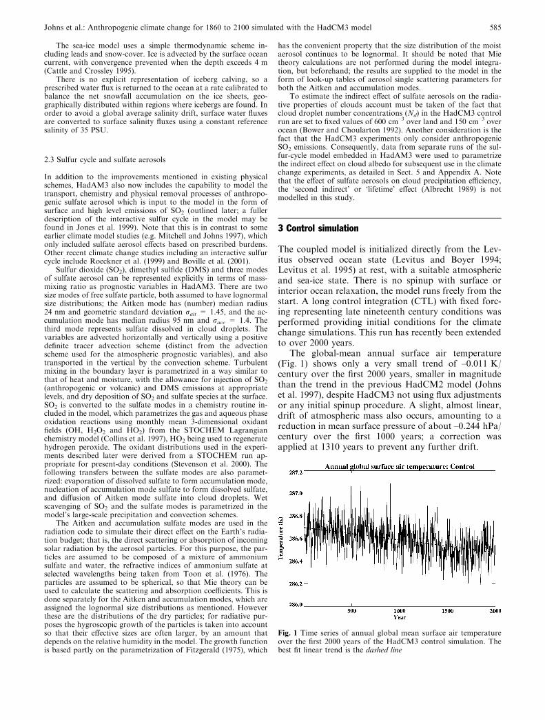
The global-mean annual surface air temperature(Fig. 1) shows only a very small trend of –0.011 K/century over the first 2000 years, smaller in magnitudethan the trend in the previous HadCM2 model (Johnset al. 1997), despite HadCM3 not using flux adjustmentsor any initial spinup procedure. A slight, almost linear,drift of atmospheric mass also occurs, amounting to areduction in mean surface pressure of about –0.244 hPa/century over the first 1000 years; a correction wasapplied at 1310 years to prevent any further drift.

Fig. 1 Time series of annual global mean surface air temperatureover the first 2000 years of the HadCM3 control simulation. Thebest fit linear trend is the dashed line

Johns et al.: Anthropogenic climate change for 1860 to 2100 simulated with the HadCM3 model 585

HadCM3 is not the only model to get very smallsurface drifts without flux adjustments. Such a resultwas previously obtained by Boville and Gent (1998) and(with smaller subsurface drifts) by Boville et al. (2001).However, those simulations were much shorter than theHadCM3 control and employed an elaborate spinupprocedure.

3.1 Mean climatology and variability

Gordon et al. (2000) describe some of the main featuresof the first 400 years of the control simulation, concen-trating on the global heat budget, ocean and sea-iceclimatology. Although some temporal drift is apparentin the deeper ocean in its water masses and circulation,the ocean surface climatology is highly stable and gen-erally well simulated, making the model suitable for thelong climate change experiments reported here.

Seasonal mean atmospheric circulation patterns canbe judged from Fig. 2, which may also be compared withHadCM2 (Fig. 10 of Johns et al. 1997). Overall thesimulation is good; probably an improvement overHadCM2 in the Southern Hemisphere thanks to higherpressure in the subtropical anticyclones and reduceddepth of the Antarctic circumpolar trough. In theNorthern Hemisphere, HadCM3’s main error is that theIcelandic low is too shallow and the gradient too slack inthe Atlantic storm track region in DJF, an error similarto but somewhat worse than HadCM2. The NorthPacific storm track perhaps extends too far to the east

compared to the analyses. Pressure is considerably toohigh in JJA and particularly DJF over the Arctic, withcorrespondingly rather low pressure over Asia in DJF.The Asian monsoon trough is well captured in themodel, however, as are the subtropical ocean highpressure systems.

In general, the model does a good job of capturingthe patterns of mean seasonal precipitation for DJF andJJA when judged against the CMAP climatology (Xieand Arkin 1997), illustrated in Fig. 3 and 4. At mostlatitudes modelled zonal mean global precipitation cor-responds closely with CMAP in both seasons. Theagreement over land (Fig. 3c, d), where the climatologyis more reliable, is particularly good, giving confidencein the model physics. The split zonal-mean maximum inthe tropics in DJF and strong peak in JJA are repro-duced quite well (Fig. 3a, b), though in JJA the modeltends to shift the peak precipitation slightly equator-wards and there is rather a split ITCZ (inter-tropicalconvergence zone) response over the W Pacific ocean(Figs. 3f, 4b), a common problem in coupled models.While the modelled zonal mean precipitation over theSouthern Ocean appears rather high (Fig. 3e, f), theCMAP reconstruction here is subject to larger uncer-tainty; the agreement is better in southern summer whenobservations are more abundant.

More detailed examination of the precipitation dis-tribution (Fig. 4) supports the view that the model isgenerally realistic, but some deficiencies are apparent.In both seasons the model tends to overdo the precipi-tation in the eastern tropical Atlantic/Gulf of Guinea,

Fig. 2a–d Seasonal average (DJF and JJA) mean sea level pressure (hPa) simulated for years 371–610 in the HadCM3 control run,compared with mean UK Meteorological Office operational analyses for the period May 1983 to September 1995


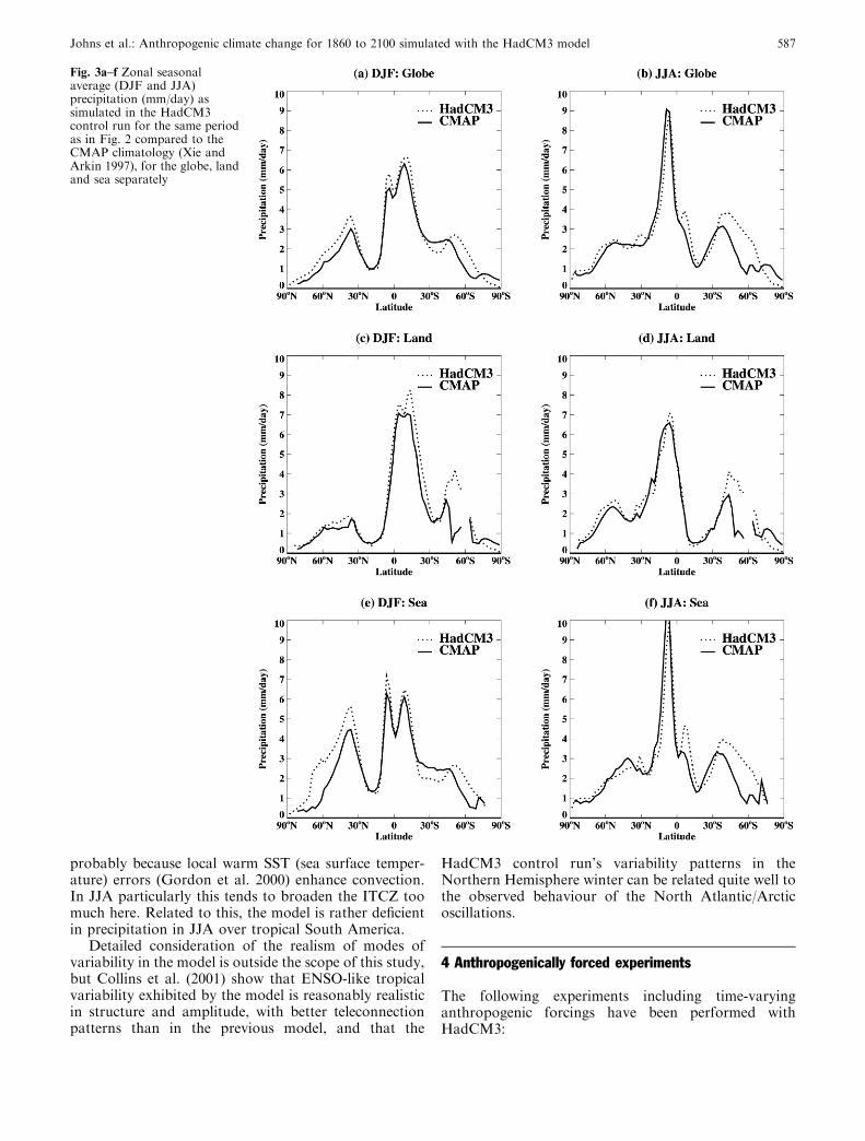
probably because local warm SST (sea surface temper-ature) errors (Gordon et al. 2000) enhance convection.In JJA particularly this tends to broaden the ITCZ toomuch here. Related to this, the model is rather deficientin precipitation in JJA over tropical South America.

Detailed consideration of the realism of modes ofvariability in the model is outside the scope of this study,but Collins et al. (2001) show that ENSO-like tropicalvariability exhibited by the model is reasonably realisticin structure and amplitude, with better teleconnectionpatterns than in the previous model, and that the

HadCM3 control run’s variability patterns in theNorthern Hemisphere winter can be related quite well tothe observed behaviour of the North Atlantic/Arcticoscillations.

4 Anthropogenically forced experiments

The following experiments including time-varyinganthropogenic forcings have been performed withHadCM3:

Fig. 3a–f Zonal seasonalaverage (DJF and JJA)precipitation (mm/day) assimulated in the HadCM3control run for the same periodas in Fig. 2 compared to theCMAP climatology (Xie andArkin 1997), for the globe, landand sea separately


1. G92, forcing from observed rises in well-mixedGHGs (WMGHGs) only from 1859 to present-day,thereafter the IS92a scenario for WMGHGs up to2100

2. A92, forcing from rises in WMGHGs as in G92, plusestimates of past changes in tropospheric ozoneconcentration and sulfur emissions, extended from1990 to 2100 according to an adapted scenarioloosely based on IS92a emissions

3. GB2, as G92, with forcing due to WMGHGs onlybut using the B2 scenario after 1990 instead of IS92a

4. A1FI, A2, B2, B1, forcing changes from observedrises in WMGHGs to present as G92 plus estimatesof past changes in tropospheric and stratosphericozone concentration and sulfur emissions, extendedfrom 1990 to 2100 according to SRES A1FI, A2,B2 and B1 scenarios (Nakicenovic et al. 2000) withestimated/modelled stratospheric ozone recovery

G92 was initialized from year 100 of the control run,A1FI and B1 from year 470, while the remainingexperiments were initialized from year 370. A1FI and B1are identical experiments up to 1989, and similarly A2and B2.

Results from the A92 experiment can be obtainedfrom the IPCC Data Distribution Centre website athttp://ipcc-ddc.cru.uea.ac.uk/, where it is referred to asthe HC3AA integration, but as the scenario is not stan-dard it is not discussed further in this study. We con-

centrate here on the other six experiments: G92, GB2,A1FI, A2, B2 and B1, particularly the four SRES cases.

A number of research groups have recently carriedout SRES scenario experiments (mostly the A2 and B2cases) with other coupled models (Stendel et al. 2000;Dai et al. 2001; Noda et al. 2001; Nozawa et al. 2001;Mahlman 2001); results from these as well as the presentstudy are summarized in the IPCC 2001 report (Cubaschet al. 2001).

5 Emissions, concentrations and radiative forcings

5.1 Well-mixed greenhouse gases

Concentration data for ‘well-mixed greenhouse gases’are input separately to the model for the three principalgases CO2, CH4 and N2O, and also for a subset of thehalocarbon species estimated to be the next largestcontributors to anthropogenic radiative forcing in therecent past and next 100 years. These were CFCl3(‘‘CFC-11’’), CF2Cl2 (‘‘CFC-12’’), CF2 ClCFCl2 (‘‘CFC-113’’), CHF2 Cl (‘‘HCFC-22’’), CF3CFH2 (‘‘HFC-134a’’) and C2HF5 (‘‘HFC-125’’). They were assumed tohave zero concentration until 1950, 1950, 1980, 1970,1990 and 1990 respectively, with histories before 1990taken from Table 2.5 of Shine et al. 1990. Note that,unlike some other models (e.g. CSM; Boville et al. 2001)that do represent their spatial variation, we regard all

Fig. 4a, b Seasonal average (DJF and JJA) precipitation in the HadCM3 control run for the same period as in Fig. 2 (contours at 1, 2, 5,10, 20 mm/day; values above 5 mm/day shaded), and c, d differences relative to the CMAP climatology (Xie and Arkin 1997) (contours at–5, –2, –0.5, 0, 0.5, 2, 5 mm/day; negative values shaded)


these species as completely well mixed for convenience,although some actually have significant variations overthe model domain (at least in the stratosphere).

For the historical period, CO2, CH4 and N2O were asspecified in the IPCC 1995 report (Schimel et al. 1996;T. Wigley personal communication) based on calcula-tions with the Bern model (Joos et al. 1996).

For the future scenario part of the experiments CH4,HFCs and HCFC-22 concentrations were calculatedfrom a continuous run of an updated version of a 2-Dchemistry transport model (‘‘TROPOS’’) used by Hough(1991). This model runs with fixed transport, and cli-matologies for temperature and humidity. It was drivenusing SRES A1FI, A2, B2 and B1 scenario emissions(Nakicenovic et al. 2000) together with estimates ofnatural emissions for methane from IPCC 1995 (Schimelet al. 1996), while CO2 and N2O data were supplied fromsources working in the SRES scenario developmentprocess (M. Prather personal communication). We ad-justed output GHG values slightly near 2000 to matchobservational estimates and avoid discontinuity with thehistorical part of the scenario. In the G92 experiment,concentration values for GHGs after 1990 were insteadtaken directly from IPCC 1995 (Tables 2.5d, 2.5e inSchimel et al. 1996). CFCs and other chlorine and bro-mine-containing compounds were calculated in a boxmodel to give CFC concentrations and the time-depen-dent effective chlorine loading of the troposphere.

The GHG concentration data used to drive the A1FI,A2, B2/GB2 and B1 scenario experiments are summa-rized in Table 1a, b. G92 differs from these only slightlyup to 1990.

The total GHG forcing at 2000 relative to pre-in-dustrial is about 2.34 W/m 2 in the B2 experiment (andsimilar in others), towards the lower end of the IPCCestimated range (Table 3a). Of this, 65% comes fromCO2 and 35% from ‘minor’ gases, CFCs and otherhalocarbons accounting for about 12%. In the future,the fractional contribution of minor GHGs falls signif-icantly, to 22% and 21% in A2 and B2 respectively by2100, by which time the halocarbon contribution to thetotal GHG forcing (which spans a range of 7.94 W/m2

for A1FI down to 4.22 W/m2 for B1; Table 3b) is evensmaller (around 5% or less), although the absoluteforcing from halocarbons shows little change.

The total change in radiative heating from 2000 to2100 for those WMGHGs included is within about0.1 W/m2 of the sum of the values given in Ramaswamyet al. (2001). The small difference arises from a combi-nation of slight discrepancies between the concentra-tions of GHGs used in the model compared to the IPCCestimates for the present-day period, the use of a pre-liminary version of the SRES emissions scenarios (aswas the case for other studies in the IPCC 2001 Report),and different radiation schemes used to calculate theimplied forcings.

Table 1a Greenhouse gas concentrations input to the model versus simulated year, for the historical period 1859–1990 followed by theSRES A2 scenario. Entries left blank and intermediate years are linearly interpolated from the given data points

Year CO2

(ppmv)CH4

(ppbv)N2O(ppbv)

CFC-11(pptv)

CFC-12(pptv)

CFC-113(pptv)

HCFC-22(pptv)

HFC-125(pptv)

HFC-134A(pptv)

1859 286.1 878 280.1 0 0 0 0 0 01875 288.81890 294.3 9471900 295.91917 302.21920 10321935 309.61940 10981950 310.9 290.0 0 01957 11911960 316.9 18 301965 294.21970 325.7 60 120 01980 338.9 173 01984 303.71990 351.1 1718 310 263 477 77 91 0 01995 358.11998 262 533 832000 366.8 1762 318 251 523 81 165 2 342010 388.4 1874 327 206 474 72 188 5 942020 415.4 2012 338 169 430 64 151 10 1682030 448.9 2170 351 138 389 57 110 16 2372040 486.3 2353 364 113 353 51 85 23 2832050 526.9 2559 378 93 320 45 68 32 3332060 571.6 2783 392 76 290 40 31 42 4562070 620.9 3026 407 62 263 36 15 53 5852080 676.7 3295 422 51 239 32 8 66 7352090 741.9 3593 439 42 216 28 4 81 9142100 818.9 3927 455 34 196 25 2 99 1134


5.2 Tropospheric and stratospheric ozone

Tropospheric and stratospheric ozone trends are calcu-lated separately as zonal averages on the model levels,trends from one epoch to another being linearly ex-trapolated and added to a baseline climatology follow-ing Li and Shine (1995) but with a number of alterations.The more significant alterations are intended to repre-sent ‘‘pre-industrial’’ conditions (the 1960s and early1970s, not 1765 as conventional for other gases) byfilling in the Antarctic ozone hole and elsewhere apply-ing smaller changes based on SAGE (StratosphericAerosol and Gas Experiment) data (Wang et al. 1996).Future concentrations of stratospheric ozone were esti-mated assuming chlorine and bromine emissions de-crease as set out in the Montreal Protocol. Troposphericozone concentrations were calculated using runs of thethree-dimensional global chemical transport modelSTOCHEM (Collins et al. 1997, 1999) to derive inter-polated trends over the experimental period. AppendixB gives further details of the methodology used to

compute the tropospheric and stratospheric ozonetrends (see also Tett et al. 2002). Climate change canaffect ozone predictions (Johnson et al. 1999; Stevensonet al. 2000). For the A2 and B2 scenarios only, this isallowed for approximately by using future climates,derived from the HadCM3 G92 run, in STOCHEM.This was not the case for A1FI, the 1989–90 (i.e. presentday) climate from the B2 run being used instead, in or-der to make the forcing in A1FI more similar to corre-sponding experiments being conducted by othermodelling groups. Further details of natural emissionsetc. are described in Stevenson et al. (2000).

The estimated changes in radiative forcing in themodel from 2000 to 2100 due to changes in troposphericozone are much smaller than the estimates given byRamaswamy et al. (2001) (e.g. 0.18 compared to 0.87 W/m2 for A2). There are several reasons for this. STO-CHEM gave about a 15% smaller change in tropo-spheric ozone abundances for A2 than the values usedby Ramaswamy et al. (2001); see also Prather et al.(2001). In addition, the ozone concentrations in Prather

1b. As Table 1a, but for the SRES B1, B2 and A1FI scenarios 1990–2100. Note that the CFC concentrations are identical to A2 in allthese scenarios so are omitted in this table

Year CO2 (ppmv) CH4 (ppbv) N2O (ppbv) HCFC22 (pptv) HFC125 (pptv) HFC134A (pptv)

B1 1990 351.1 1700 308 97 0 11995 358.22000 367 1754 316 172 1 202010 386.5 1813 324 250 3 622020 409 1869 334 215 9 1162030 433 1896 342 131 17 1712040 457.7 1883 350 81 25 2292050 481.9 1844 358 44 34 3002060 501.7 1809 365 19 43 3572070 515.8 1781 369 8 49 3852080 524.2 1734 373 3 53 3982090 529.8 1672 376 1 56 4012100 531.4 1594 377 1 58 394

B2 1990 351.1 1718 310 91 0 01995 358.12000 366.8 1745 318 164 2 352010 387.9 1821 327 188 6 982020 410.7 1927 335 150 11 1682030 433 2041 342 100 19 2592040 454.8 2165 347 52 27 3572050 476.9 2299 352 24 38 4742060 499.5 2395 356 11 49 5872070 523.2 2445 358 5 60 6842080 547.9 2476 361 2 70 7772090 574.8 2499 362 1 80 8732100 603.7 2521 364 0.5 90 977

A1FI 1990 351.1 1700 308 97 0 11995 358.12000 366.4 1707 316 172 1 202010 386.9 1763 325 249 3 652020 414 1874 336 215 11 1382030 450.5 2048 348 132 23 2482040 497.5 2277 363 84 38 3702050 556 2528 381 47 56 5172060 623 2730 399 21 75 6592070 694.5 2884 416 9 92 7582080 770.8 3025 433 4 105 8102090 848.5 3155 449 2 116 8322100 925.5 3263 465 1 123 829


et al. (2001) are thought to be about 25–30% too high(due to an error they included a contribution from in-creases in stratospheric ozone). In the B2 and A2 sce-narios, the calculations here, unlike those in Prather etal. (2001), took into account changes in temperature andhumidity estimated from an earlier climate change ex-periment (see earlier), further reducing the concentra-tions, see Johnson et al. (2001). The net effect is that thechange in radiative forcing due to changes in tropo-spheric ozone from 2000 to 2100 in Prather et al. (2001)may be an overestimate by about a factor of two.However, there is a further reduction in the contributionto the discrepancy arising from the interpolation ofozone changes from STOCHEM onto the coarser ver-tical resolution of HadCM3, in which changes at thetropopause were set to zero. Due to the discretizationand interpolation of trends in the vertical, the result wasto reduce the ozone changes immediately below thetropopause, precisely the region in which changes wouldhave their strongest radiative effect (Forster and Shine1997). Thus the values here are about 0.2 W/m2 in theA2 and A1FI scenarios, smaller than the Prather et al.(2001) values, even allowing for the possible shortcom-ings in their estimate.

To evaluate the implied forcing from imposed ozonechanges presents some difficulties in that the radiativeforcing concept relates to the flux change at the tropo-pause, but ozone depletion at and above this level causespotentially strong adjustments in stratospheric temper-atures system ownward tongwave (LW) flux at the tro-popause. The adjustment of the stratosphere to aninstantaneous change of ozone would take place on atime-scale of a few months and one should let theseadjustments reach equilibrium before evaluating theimplied forcing on the troposphere and climate systembelow.

In this study, we calculated the forcing by two al-ternative methods. Our preferred method is to calculatethe forcing interactively in the coupled model by makingdouble calls to the radiation scheme with both theevolving state and a reference control (unperturbed)state (Tett et al. 2002), and estimating the forcing as thedifference between the two radiative calculations at thediagnosed tropopause averaged over a few years ofmodel integration. We used this method for the years2000, 2050 and 2100 when the stratospheric ozonechanges are most significant.

The alternative method of estimating ozone forcinginvolves first calculating the stratospheric radiativeheating/cooling rates using the control run (unperturbedforcing), assuming the stratosphere to be in radiativeand dynamical balance. We here assume that underimposed ozone changes the dynamical changes arenegligible. Hence to maintain equilibrium, radiativeheating rates must also remain unchanged. To achievethis, iterative calculations were performed off-line fromthe model experiments themselves, in which strato-spheric temperatures were adjusted under the imposedozone changes until the radiative heating rates return to

the reference values. This method is referred to as the‘fixed dynamical heating’ (FDH) approximation (e.g.Ramanathan and Dickinson 1979). Ozone distributionsfor selected years of the coupled model experiments wereiterated using this method for monthly mean states froma two year section of the control run and the radiativeflux changes at the tropopause averaged over the twoyears to derive the approximated radiative forcing in theexperiments. We used this method for the years 1900,1950, 1975, 1990, 2000, 2050 and 2100, allowing us tocompare with the interactive method, and also allowingdirect comparison with earlier studies that used theFDH method.

The FDH approximation could be unrealistic if sig-nificant dynamical adjustments also occur in thestratosphere in response to ozone changes. We can judgethis to some extent by examining the radiative and dy-namical balance in the forced experiments themselves(see Sect. 6), although other forcings and feedbacks mayamplify or reduce these dynamical changes.

Our preferred method of calculating the ozone forc-ing interactively (Tett et al. 2002) appears to yield ahigher cooling effect from stratospheric ozone depletionthan the FDH method and therefore a lower netwarming effect overall in general (Table 3c). However,the difference between the two forcing estimates is atmost a few tenths of a W/m2 in the A1FI, A2, B2 and B1scenarios thoughout the twenty first century, a minoruncertainty relative to the total forcing.

5.3 Sulfur and sulfate aerosols

As mentioned in Sect. 2, the direct radiative effect ofsulfate aerosols is determined explicitly from the an-thropogenic aerosol concentration and physical state ofthe atmosphere. The effect is computed in both the clear-sky and cloudy portions of a grid box but is much lesssignificant in the presence of cloud.

To determine the indirect sulfate forcing effect, amore complex calibration procedure was required asdescribed in Appendix A. The anthropogenic forcingchanges were applied in the HadCM3 experiments viaspecified cloud albedo perturbations based on priorcalibration experiments performed separately usingHadAM3, which had the natural and anthropogenicemissions included with present-day climate. Thismethod avoids the need to include the natural sulfurcycle explicitly in the control and forced HadCM3 ex-periments, which would have been more expensivecomputationally. The technique produces an indirectaerosol forcing distribution in HadCM3 similar to thatin the HadAM3 calibration runs but typically of about70% of the magnitude, the discrepancy arising from atleast three sources:

1. Limitations of the parametrized method; e.g. runninginto limits on the cloud effective radius, and so beingunable to produce the desired amount of forcing, and


the fact that the simple measure of cloud albedo usedmay not accurately track the (complex) changes incloud radiative properties which actually produce theforcing.

2. Problems with time-averaging such that the forcingassociated with timestep-by-timestep changes incloud albedo (as in the HadAM3 calibration runs) isnot the same as that produced by an annual-mean ofthese albedo changes (as used in the HadCM3experiments).

3. Differences in the meteorology in the simulations,particularly in the distribution of clouds which willproduce differences in the forcing locally.

Given the large uncertainty in estimates of the indi-rect effect (e.g. Ramaswamy et al. 2001), this imperfectmethod was nevertheless considered adequate for thisstudy.

The variations in sulfate aerosol burdens andforcings in A1FI, A2, B2 and B1 are illustrated in

Fig. 5, with linear interpolation between the calibra-tion years which are marked with symbols. One yearre-runs were performed with additional radiationcomputations to derive these forcings. The globalannual mean (anthropogenic) aerosol burden at 2000is approximately 0.25 Tg(S), from emissions of69 Tg(S) per annum, implying a burden/emissions ra-tio of 1.32 days. This ratio is clearly too low; forexample the average of the same ratio among 11models tabulated by Penner et al. (2001) is 2.9 days.The main reason for the low aerosol loading is thatthe rates of dry and wet deposition are too rapid inthis version of the model. However, it is also relevantthat anthropogenic sulfur emissions produce lessaerosol (per unit mass of S emitted) than naturalemissions, for reasons discussed by Penner et al.(2001), who quoted a range of 0.8 to 2.9 days for thisratio with respect to anthropogenic SO2 emissions.

In accordance with the emissions scenarios, theglobal-mean burden and forcing both rise sharply in

Fig. 5 Time series of a global mean anthropogenic sulfate burden;b direct and indirect sulfate forcing; c global annual mean turnovertime in the atmosphere (i.e. anthropogenic sulfur burden divided byemissions); and d normalized direct and indirect forcing (i.e. forcingdivided by burden); for the A1FI, A2, B2 and B1 experiments. Note

that the forcings and burdens represent data computed from singleyears of the experiments only, not continuously throughout thesimulations. The indirect forcing as diagnosed in the coupledexperiments is typically about 30% weaker than that diagnosed inseparate offline calculations using HadAM3 (see text)


A1FI and A2, peaking at 2030 (between the 2000 and2050 data points plotted in Fig. 5) before falling back at2100. (Regional breakdowns of the anthropogenic sulfuremissions in the A1FI, A2, B2 and B1 scenarios bybroad world economic regions are given in Table 2). Theglobal burden in B2 (Fig. 5a) remains quite level overthe twenty first century despite a marked decrease inemissions from 69.0 to 47.3 Tg[S]/year between 2000and 2100, and in A2 the burden at 2100 is considerably

higher than 2000 despite the reduced emissions(60.3 Tg[S]/year at 2100).

A pronounced rise in the effective global mean turn-over time is thus apparent through the simulations(Fig. 5c). The most significant factor is the migrationthrough time of emissions to subtropical and tropicalregions where oxidant concentrations are much greaterthan in mid-latitudes and therefore more efficient forsulfate production – the rise is a consequence primarily

Table 2 Sulfur emissions (Mt(S)/year) by world economic regions at decadal intervals for the preliminary SRES scenarios B2 and A2(Steve Smith personal communication), and the B1 marker and A1FI illustrative scenarios (Nakicenovic et al. 2000)

Year OECD 90 FSU/EE = REF China/CPA + SE Asia = ASIA Lat Am + Afr/Mid E = ALM Shipping Total

B1 1990 22.7 17.0 17.7 10.5 3.0 70.92000 17 11.0 25.3 12.8 3.0 69.02010 11.8 9.0 29.0 21.2 3.0 73.92020 7.9 7.7 29.1 26.8 3.0 74.62030 5.4 6.9 29.2 33.7 3.0 78.22040 3.6 7.0 27.6 37.4 3.0 78.52050 2.5 6.5 21.4 35.6 3.0 68.92060 2.0 5.6 15.3 29.9 3.0 55.82070 2.0 4.6 10.7 24 3.0 44.32080 2.1 3.9 7.7 19.5 3.0 36.12090 2.3 3.0 5.8 15.7 3.0 29.82100 2.6 2.5 4.2 12.6 3.0 24.9

B2 1990 22.7 17.9 11.9 + 6.0 = 17.9 4.8 + 6.3 = 11.1 3.0 72.62000 18.6 11.4 15.3 + 8.1 = 23.4 5.3 + 7.3 = 12.6 3.0 69.02010 13.4 9.5 18.6 + 10.7 = 29.3 5.7 + 7.3 = 13.0 3.0 68.22020 8.1 5.8 21.7 + 12.0 = 33.7 7.3 + 7.2 = 14.5 3.0 65.02030 3.9 2.4 21.6 + 13.9 = 35.5 7.1 + 8.0 = 15.1 3.0 59.92040 3.4 0.7 19.5 + 15.8 = 35.3 6.8 + 9.6 = 16.4 3.0 58.82050 3.0 0.6 17.5 + 15.7 = 33.2 6.4 + 11.0 = 17.4 3.0 57.22060 2.6 2.4 10.9 + 15.9 = 26.8 6.5 + 12.4 = 18.9 3.0 53.72070 2.7 2.5 7.8 + 16.4 = 24.2 6.0 + 13.6 = 19.6 3.0 51.92080 2.9 2.8 5.7 + 15.7 = 21.4 5.2 + 13.8 = 19.0 3.0 49.12090 3.2 3.3 5.2 + 15.0 = 20.2 4.4 + 14.1 = 18.5 3.0 48.02100 3.6 3.7 4.9 + 14.8 = 19.7 3.4 + 13.8 = 17.2 3.0 47.3

A2 1990 22.7 17.9 11.9 + 6.0 = 17.9 4.8 + 6.3 = 11.1 3.0 72.62000 18.6 11.4 15.3 + 8.1 = 23.4 5.3 + 7.3 = 12.6 3.0 69.02010 9.4 11.5 18.4 + 16.0 = 34.4 8.2 + 8.1 = 16.3 3.0 74.72020 9.9 12.3 21.6 + 28.3 = 49.9 11.7 + 12.6 = 24.3 3.0 99.52030 10.4 12.3 20.2 + 34.7 = 54.9 12.9 + 18.4 = 31.3 3.0 111.92040 10.5 11.3 17.5 + 33.8 = 51.3 11.2 + 20.9 = 32.1 3.0 108.12050 10.6 10.5 15.1 + 32.9 = 48.0 9.7 + 23.7 = 33.4 3.0 105.42060 9.8 8.1 13.0 + 24.6 = 37.6 6.3 + 21.5 = 27.8 3.0 86.32070 9.2 6.1 11.2 + 18.4 = 29.6 4.1 + 19.7 = 23.8 3.0 71.72080 9.5 4.9 9.8 + 15.3 = 25.1 3.2 + 18.7 = 21.9 3.0 64.22090 10.6 4.0 8.6 + 14.1 = 22.7 2.9 + 18.7 = 21.6 3.0 61.92100 11.8 3.2 7.5 + 13.0 = 20.5 2.7 + 19.1 = 21.8 3.0 60.3

A1FI 1990 22.7 17.0 17.7 10.5 3.0 70.92000 17.0 11.0 25.3 12.8 3.0 69.02010 13.9 10.3 38.8 14.9 3.0 80.82020 4.7 10.5 52.7 16.1 3.0 86.92030 4.0 13.3 57.1 18.6 3.0 96.12040 4.2 13.4 51.9 21.5 3.0 94.02050 5.1 10.7 37.0 24.7 3.0 80.52060 5.2 5.8 24.3 17.9 3.0 56.32070 5.7 3.1 17.0 13.8 3.0 42.62080 6.5 2.4 15.1 12.4 3.0 39.42090 7.3 2.5 14.6 12.4 3.0 39.82100 8.0 2.6 14.1 12.4 3.0 40.1

OECD90, OECD group developed countries; FSU/EE, FormerSoviet Union and Eastern Europe, CPA Centrally Planned Asia;Lat Am Latin America; Afr/Mid E Africa and Middle East. Thefull definitions of the world regions are given on pages 332–333 ofNakicenovic et al. (2000). Note that the emissions actually used at

1990 in the HadCM3 experiments B1 and A1FI were identical tothose in B2 and A2 for simplicity in conducting the experiments,rather than the slightly different values tabulated (italicized) whichreflect revisions between the preliminary and final versions of therespective emissions scenarios


of the geographical characteristics of the emissions sce-nario, therefore. It is also relevant that there is less wetdeposition in the subtropics. There is also a slow accu-mulation of sulfate in the stratosphere in the model, butseparate HadAM3 experiments with emissions fields forvarious epochs (but present-day SSTs and GHG con-centrations) have shown that this is only a minor con-tributory factor. It should be noted here that variationsof oxidant concentrations in response to climate changewould be expected to modulate the burden/emissionsratio as well, but we do not model this effect.

In B2 the direct forcing remains fairly constant be-tween 2000 and 2100 (Fig. 5b) like the burden, but theindirect forcing reduces significantly. To a good ap-proximation the direct forcing scales linearly with theglobal sulfate burden, but this is clearly not the case forthe indirect effect. The normalized indirect forcing (i.e.forcing per unit sulfate burden; Fig. 5d) weakens by alarge factor (more than a factor of 4 between 1860 and2100 in B2) as the sulfate burden increases. This is ex-pected partly because the sensitivity of cloud to addingfurther sulfate at a given location decreases with in-creasing aerosol. In our formulation of the effect, giventhat any points where the albedo perturbation wouldgive rise to a cloud albedo greater than unity have theiralbedos limited, one would also expect this to compoundthe drop-off of the normalized indirect forcing at highaerosol concentrations, e.g. at 2050 in A2. The differencein normalized indirect forcing between 2000 and 2050/2100 in B2 (despite similar global sulfate burdens) isprobably mainly due to the main areas of pollutionmoving to lower latitudes where layer cloud is lessabundant.

It may seem a little surprising at first sight that thefossil-fuel-intensive scenario A1FI gives rise to a lowersulfate burden at 2050 than A2, with consequentlyweaker aerosol forcing. Indeed, at 2100 the A1FI aero-sol burden is lower even than in the B2 case. However,A1FI is an amalgamation of the A1C and A1G sce-narios (Nakicenovic et al. 2000). Of these, A1C assumesheavy use of coal, but burned using ’clean’ technologiesthat reduce sulfur emissions; while A1G assumes heavyuse of oil and gas, fuels which contain less sulfur.

5.4 Net radiative forcing

Our simulations do not take changes in black carbonand organic carbon into account. Their combinedchange in radiative forcing tends to cancel in the globalaverage, although this is unlikely to be the case locally.The net global mean forcing from 2000 to 2100 fromblack carbon and organic carbon combined has beenestimated to be about –0.20 W/m2 in A2 and A1FI(Ramaswamy et al. 2001). The sum of the change inforcings from 2000 to 2100 (excluding the indirect effectof sulfate aerosols) in the model is close to the sum of theanthropogenic components given in Houghton et al.(2001), Appendix II. This is because there is an

additional model contribution from the recovery ofstratospheric ozone (Appendix B) which compensatesfor the shortfall in the contribution from troposphericozone and our neglect of black and organic carbon.

The future rate of increase in net radiative forcing inthe GB2 scenario is similar to that over recent decades(Fig. 6), and reaches about 4.5 W/m2 by 2100. In otherwords, WMGHG forcing in B2 continues the recenttrend. If only WMGHGs are included in the forcing(GB2 compared to B2), the net radiative forcing is about1.0 W/m2 higher in 1990, and 1.3 W/m2 higher in 2000as the negative forcing from stratospheric ozone deple-tion peaks (Table 3a), but B2 and GB2 then convergeagain at the end of the twenty first century (Fig. 6). Thisfollows partly from the gradual decrease in sulfuremissions and consequent weakening of that forcing inB2 in the second half of the century (Table 2, Fig. 5b),and partly from the increasing contribution to the an-thropogenic forcing from ozone in all SRES scenarios,including B2 (Table 3b).

The forcings in A1FI and A2 diverge sharply from B2in the 2020s and 2040s respectively (Fig. 6), followingthe rapid increase in the CO2 and other GHG emissionsrelative to B2 at those times (Table 1), while B1 divergesgradually from B2 throughout the twenty first century.Initially, the forcing increases much faster in A1FI be-cause GHG emissions increase faster, and sulfur emis-sions are lower. Towards the end of the twenty firstcentury, however, this trend is reversed—sulfur and CO2

emissions rates are then similar in both scenarios, butthe emission rates of some trace gases (e.g. CH4, HFC-134a) become much higher in A2 (inferred fromTable 1). By 2100, the net heating relative to preindus-trial values reaches 7.0 and 7.8 W/m2 in A2 and A1FIrespectively (Table 3b), compared to 6.7 W/m2 in theold G92 (WMGHGs-only) scenario.

Fig. 6 Time series of annual global mean total forcing at thetropopause computed for the HadCM3 experiments G92, GB2,A1FI, A2, B2 and B1 over the period 1859–2100, each relative totheir average over the period 1880–1920. Effects of greenhousegases, direct and indirect sulfate aerosol forcing, tropospheric andstratospheric ozone changes are included


The increase in forcing is slowest in the B1 scenario,which assumes small energy demand, improvements inenergy efficiency and the development of non-fossil fuelenergy sources (Nakicenovic et al. 2000). Even in thiscase, however, the forcing reaches 4.0 W/m2 by 2100(Table 3b).

6 Climate change response

In much of the analysis in this section we concentrate on30-year averages, of annual and seasonal mean (DJFand JJA) variables in order to enhance the signal-to-noise ratio. Two future periods, the ‘2040s’ (the 30-yearperiod from December 2029 to November 2059) and the‘2080s’ (similar but 2069 to 2099) are chosen. Differencesare constructed either relative to a 240-year period ofCTL parallel to the forced experiments, or relative to a30-year present-day period, the ‘1980s’ (as before but1969 to 1999). In order to estimate noise we use thestandard deviation of successive 30-year averages fromCTL (see Collins et al. 2001 for more detail on thevariability in CTL), and estimate significance levels as-suming 30-year average signals sampled from the forcedexperiments are normally distributed about a meansignal level with standard deviation as estimated fromCTL, i.e. with no change of variance in response toforced climate changes.

However, we first consider trends of annual meanquantities over the entire simulation period.

6.1 Global warming, sea level, and sea-ice trends

Of the six scenario experiments G92, GB2, A1FI, A2, B2and B1 the first two (GHGs only) exhibit overall globalwarming from 1900 to present somewhat above theobserved, whereas the latter four (including other an-thropogenic forcings) agree much better with the ob-served change, represented here by an updated versionof the blended MOHSST6-UEA SST and surface airtemperature dataset (Parker et al. 1994) (Fig. 7a). Notehowever that the rate of global warming in recent de-cades is similar in all cases (A1FI, A2, B2 and B1 beingidentically forced up to 1989). It is plausible that theinclusion of all anthropogenic forcings in the A1FI, A2,B2 and B1 cases is more realistic in representing thetwentieth century record, but it is not our purpose todeal with detailed attribution analysis using these sim-ulations—that question is addressed by Tett et al.(2002). For the sake of discussion of the future forcedresponses we simply assume that the results are a rea-sonable guide to the future given the scenario inputs, buta number of caveats are also discussed later.

Relative to 1900, simulated global warming spans arange of about 1.5 to 2.5 K at 2050 rising to 2.6 to 5.3 Kin 2100. The upper envelope is defined by G92 and GB2up to about 2050, but A1FI warms most thereafter, whilethe lower envelope is provided by A2 up to about 2030and thereafter by B1. The A2 and A1FI warmings riseparticularly steeply in the mid twenty first century, fol-lowing the increase of emissions discussed in Sect. 5. Over

b HadCM3 global mean forcings at 2100 relative to pre-industrial values in the four SRES experiments A1FI, A2, B2 and B1. Ozoneestimates are from the interactive method. The stratospheric ozone forcing contributes +0.17 W/m2 in all four scenarios (see Appendix B)

Future forcings(W/m2)

WMGHGs(total)

WMGHGs(minor)

Sulfate(direct)

Sulfate(indirect)

Ozone(total)

Net

A1FI 7.94 1.45 –0.17 –0.61 0.66 7.82A2 7.47 1.64 –0.24 –0.79 0.60 7.04B2 5.29 1.10 –0.18 –0.71 0.49 4.89B1 4.22 0.72 –0.10 –0.50 0.39 4.01

Table 3a Comparison of HadCM3 global mean present day (2000) forcing relative to pre-industrial values with IPCC 2001 (Ramaswamyet al. 2001) estimated ranges for present-day. The IPCC WMGHG forcings are the quoted central estimates, which have an uncertainty of10%. HadCM3 figures are from the B2 experiment. The ozone forcing and its range are as estimated using the interactive method (notethat the FDH method gives a substantially lower stratospheric effect, within the IPCC range)

Present forcings(W/m2)

WMGHGs(total)

WMGHGs(minor)

Sulfate(direct)

Sulfate(indirect)

Ozone(Tropospheric)

Ozone(Stratospheric)

HadCM3 2000 2.34 0.84 –0.18 –0.91 [0.19, 0.24] [–0.59, –0.65]IPCC 2001 2.43 0.97 [–0.2, –0.8] [–0.3, –1.8] [0.25, 0.50] [–0.09, –0.25]

c Comparison of two alternative estimates of present and future ozone forcing in HadCM3 for 2000, 2050 and 2100 calculated using adiagnostic method in the model allowing interactive adjustment of the stratosphere, and the fixed dynamical heating method (FDH)

Ozone Forcing(W/m2) Interactive/FDH extimates

A1FI A2 A2 B1

2000 –0.38/+0.24 –0.37/+0.23 –0.41/+0.22 –0.34/+0.212050 0.41/0.60 0.29/0.48 0.29/0.42 0.30/0.352100 0.66/0.76 0.60/0.63 0.49/0.46 0.39/0.31


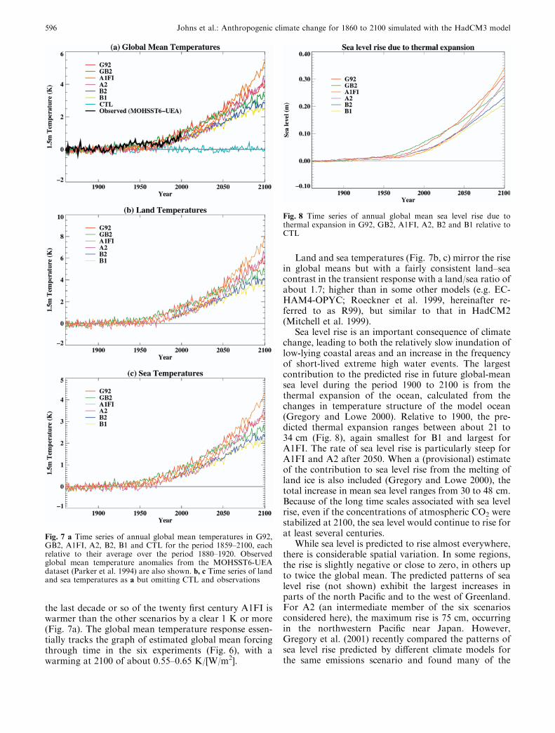
the last decade or so of the twenty first century A1FI iswarmer than the other scenarios by a clear 1 K or more(Fig. 7a). The global mean temperature response essen-tially tracks the graph of estimated global mean forcingthrough time in the six experiments (Fig. 6), with awarming at 2100 of about 0.55–0.65 K/[W/m2].

Land and sea temperatures (Fig. 7b, c) mirror the risein global means but with a fairly consistent land–seacontrast in the transient response with a land/sea ratio ofabout 1.7; higher than in some other models (e.g. EC-HAM4-OPYC; Roeckner et al. 1999, hereinafter re-ferred to as R99), but similar to that in HadCM2(Mitchell et al. 1999).

Sea level rise is an important consequence of climatechange, leading to both the relatively slow inundation oflow-lying coastal areas and an increase in the frequencyof short-lived extreme high water events. The largestcontribution to the predicted rise in future global-meansea level during the period 1900 to 2100 is from thethermal expansion of the ocean, calculated from thechanges in temperature structure of the model ocean(Gregory and Lowe 2000). Relative to 1900, the pre-dicted thermal expansion ranges between about 21 to34 cm (Fig. 8), again smallest for B1 and largest forA1FI. The rate of sea level rise is particularly steep forA1FI and A2 after 2050. When a (provisional) estimateof the contribution to sea level rise from the melting ofland ice is also included (Gregory and Lowe 2000), thetotal increase in mean sea level ranges from 30 to 48 cm.Because of the long time scales associated with sea levelrise, even if the concentrations of atmospheric CO2 werestabilized at 2100, the sea level would continue to rise forat least several centuries.

While sea level is predicted to rise almost everywhere,there is considerable spatial variation. In some regions,the rise is slightly negative or close to zero, in others upto twice the global mean. The predicted patterns of sealevel rise (not shown) exhibit the largest increases inparts of the north Pacific and to the west of Greenland.For A2 (an intermediate member of the six scenariosconsidered here), the maximum rise is 75 cm, occurringin the northwestern Pacific near Japan. However,Gregory et al. (2001) recently compared the patterns ofsea level rise predicted by different climate models forthe same emissions scenario and found many of the

Fig. 8 Time series of annual global mean sea level rise due tothermal expansion in G92, GB2, A1FI, A2, B2 and B1 relative toCTL

Fig. 7 a Time series of annual global mean temperatures in G92,GB2, A1FI, A2, B2, B1 and CTL for the period 1859–2100, eachrelative to their average over the period 1880–1920. Observedglobal mean temperature anomalies from the MOHSST6-UEAdataset (Parker et al. 1994) are also shown. b, c Time series of landand sea temperatures as a but omitting CTL and observations


regional details to be model-specific. Thus, ourconfidence in the predicted spatial patterns of sea levelrise is currently less than for temperature change pat-terns.

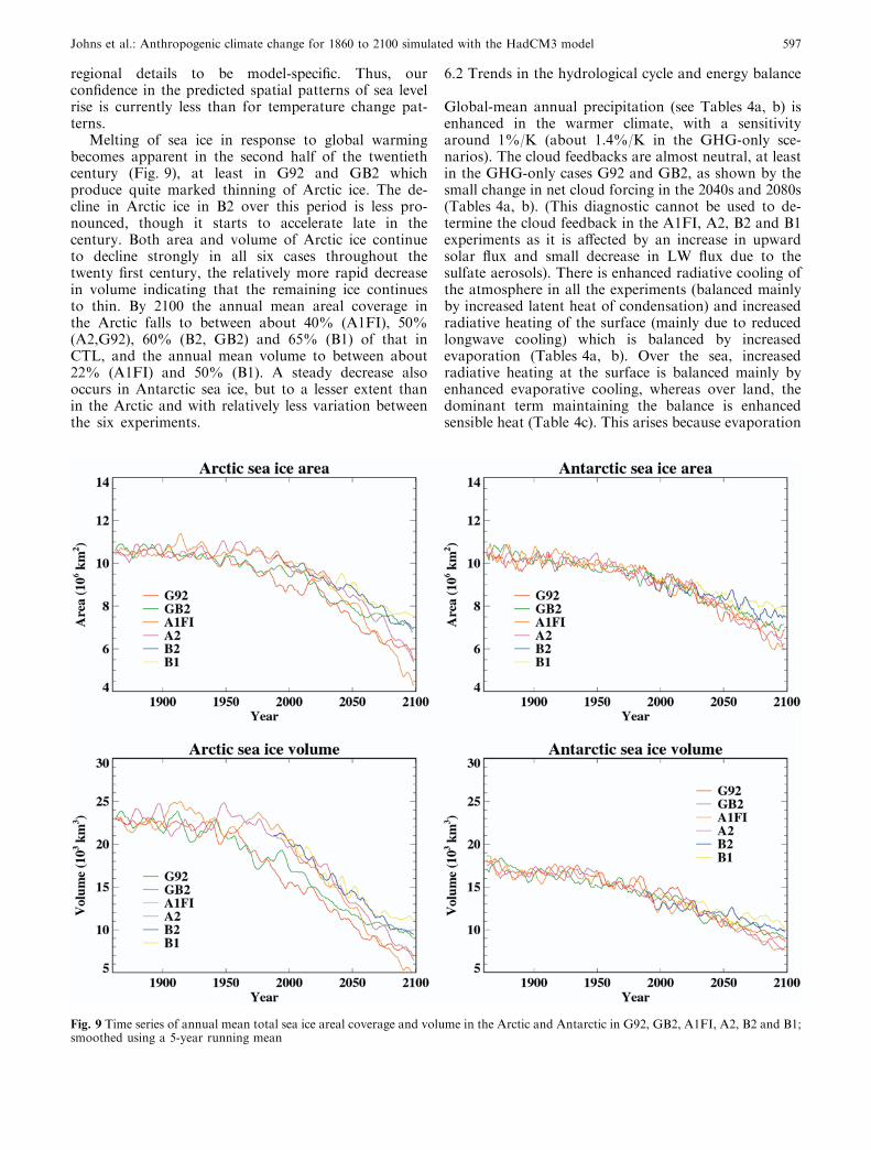
Melting of sea ice in response to global warmingbecomes apparent in the second half of the twentiethcentury (Fig. 9), at least in G92 and GB2 whichproduce quite marked thinning of Arctic ice. The de-cline in Arctic ice in B2 over this period is less pro-nounced, though it starts to accelerate late in thecentury. Both area and volume of Arctic ice continueto decline strongly in all six cases throughout thetwenty first century, the relatively more rapid decreasein volume indicating that the remaining ice continuesto thin. By 2100 the annual mean areal coverage inthe Arctic falls to between about 40% (A1FI), 50%(A2,G92), 60% (B2, GB2) and 65% (B1) of that inCTL, and the annual mean volume to between about22% (A1FI) and 50% (B1). A steady decrease alsooccurs in Antarctic sea ice, but to a lesser extent thanin the Arctic and with relatively less variation betweenthe six experiments.

6.2 Trends in the hydrological cycle and energy balance

Global-mean annual precipitation (see Tables 4a, b) isenhanced in the warmer climate, with a sensitivityaround 1%/K (about 1.4%/K in the GHG-only sce-narios). The cloud feedbacks are almost neutral, at leastin the GHG-only cases G92 and GB2, as shown by thesmall change in net cloud forcing in the 2040s and 2080s(Tables 4a, b). (This diagnostic cannot be used to de-termine the cloud feedback in the A1FI, A2, B2 and B1experiments as it is affected by an increase in upwardsolar flux and small decrease in LW flux due to thesulfate aerosols). There is enhanced radiative cooling ofthe atmosphere in all the experiments (balanced mainlyby increased latent heat of condensation) and increasedradiative heating of the surface (mainly due to reducedlongwave cooling) which is balanced by increasedevaporation (Tables 4a, b). Over the sea, increasedradiative heating at the surface is balanced mainly byenhanced evaporative cooling, whereas over land, thedominant term maintaining the balance is enhancedsensible heat (Table 4c). This arises because evaporation

Fig. 9 Time series of annual mean total sea ice areal coverage and volume in the Arctic and Antarctic in G92, GB2, A1FI, A2, B2 and B1;smoothed using a 5-year running mean


is restricted over parts of the continents, and the surfacetemperature is generally higher over the ocean than overwell-watered land, making evaporation a more efficientmeans of losing energy than sensible heat. There is an

increase in the flux of moisture from ocean to land in allexperiments.

The global sensitivity of precipitation for a givenwarming is much higher than in ECHAM4-OPYC

Table 4a Global mean radiative, energy and water fluxes in the control run (CTL) and the corresponding differences in the forcedexperiments relative to the control run for the 2040s period

Global means CTL G92 GB2 B1 B2 A2 A1FI

Atmospheric fluxes (2040s) (W/m2)SW at TOA (net) 240.42 1.86 1.79 0.30 0.55 0.40 0.67LW at TOA (up net) –240.59 –0.62 –0.75 0.63 0.47 0.80 0.70LW at TOA (up – CS) –262.16 –0.22 –0.36 1.16 1.03 1.45 1.34LW at TROP (net) –225.47 –0.92 –0.72 0.58 0.36 0.73 0.61Net radiation at TOA –0.17 1.24 1.03 0.93 1.02 1.19 1.37Net radiation at TROP 1.86 1.12 0.95 0.87 0.92 1.10 1.26SW cloud forcing –49.65 0.37 0.35 –0.30 –0.24 –0.25 –0.23LW cloud forcing 21.57 –0.4 –0.39 –0.53 –0.56 –0.65 –0.64Net cloud forcing –28.07 –0.03 –0.04 –0.84 –0.80 –0.90 –0.88Atmospheric radiative heating –101.88 –2.49 –2.22 –0.99 –1.26 –1.14 –1.38Atmospheric greenhouse effect 154.28 11.98 10.51 8.55 9.06 10.25 11.18Hydrological fluxes (2040s) (mm/day)Total precipitation 2.903 0.091 0.083 0.039 0.051 0.047 0.055Dynamic precipitation 0.723 0.021 0.020 0.010 0.013 0.015 0.017Convective precipitation 2.180 0.069 0.062 0.029 0.038 0.032 0.038Evaporation+sublimation 2.904 0.091 0.083 0.039 0.051 0.047 0.056Surface energy (2040s) (W/m2)SW (net) 164.34 –0.07 –0.24 –1.16 –1.07 –1.39 –1.38LW (emitted) –394.87 –12.60 –11.27 –7.92 –8.59 –9.45 –10.48Surface net radiation 101.71 3.72 3.25 1.91 2.28 2.33 2.75Sensible heat –16.98 0.01 0.07 0.06 0.12 0.12 0.10Latent heat –84.15 –2.62 –2.39 –1.12 –1.46 –1.35 –1.60Surface net heat flux 0.57 1.12 0.93 0.85 0.94 1.09 1.25SAT at 1.5 m (2040s) (K) 286.65 2.43 2.17 1.54 1.66 1.83 2.03

Positive fluxes indicate a net downwards flux or into the layer considered. (TOA, top of atmosphere; TROP, tropopause; SW, shortwave,LW, longwave; CS, clear-sky, SAT, surface air temperature)

b As Table 4a but global mean differences for the 2080s period

Global means CTL G92 GB2 B1 B2 A2 A1FI

Atmospheric fluxes (2080s) (W/m2)SW at TOA (net) 240.42 2.58 2.31 1.44 1.52 1.98 2.81LW at TOA (up net) –240.59 –1.00 –1.05 –0.47 –0.28 –0.08 –0.58LW at TOA (up – CS) –262.16 –0.66 –0.75 –0.01 0.24 0.62 0.05LW at TROP (net) –225.47 –1.28 –0.99 –0.26 –0.08 0.14 –0.39Net radiation at TOA –0.17 1.58 1.26 0.97 1.24 1.91 2.23Net radiation at TROP 1.86 1.41 1.14 0.87 1.11 1.72 2.00SW cloud forcing –49.65 0.41 0.36 –0.00 –0.02 0.01 0.29LW cloud forcing 21.57 –0.34 –0.29 –0.46 –0.52 –0.70 –0.62Net cloud forcing –28.07 0.07 0.07 –0.47 –0.54 –0.69 –0.33Atmos. Radiative heating –101.88 –3.57 –2.92 –2.11 –2.22 –2.66 –3.34Atmos. Greenhouse effect 154.28 18.32 14.90 11.95 13.81 18.61 21.96Hydrological fluxes (2080s) (mm/day)Total precipitation 2.903 0.123 0.099 0.076 0.077 0.094 0.112Dynamic precipitation 0.723 0.029 0.025 0.018 0.020 0.025 0.026Convective precipitation 2.180 0.094 0.075 0.058 0.057 0.069 0.085Evaporation+sublimation 2.904 0.124 0.100 0.076 0.077 0.095 0.113Surface energy (2080s) (W/m2)SW (net) 164.34 –0.69 –0.64 –1.07 –1.38 –1.85 –1.81LW (emitted) –394.87 –19.32 –15.94 –12.43 –14.10 –18.69 –22.53Surface net radiation 101.71 5.15 4.18 3.08 3.45 4.57 5.58Sensible heat –16.98 –0.19 –0.19 –0.02 –0.13 –0.12 –0.32Latent heat –84.15 –3.55 –2.87 –2.20 –2.22 –2.71 –3.23Surface net heat flux 0.57 1.41 1.12 0.86 1.11 1.74 2.02SAT at 1.5 m (2080s) (K) 286.65 3.67 3.04 2.38 2.70 3.56 4.26


(R99). The reasons for the difference are not entirelyclear, especially as only the G92 and R99 GHG exper-iments are directly comparable. On examining thechanges in these two experiments for the 2040s when theglobal mean warmings in G92 and GHG are 2.43 K and2.39 K respectively (Table 5), one finds that the increasein the net downward flux at the top of the atmosphere issimilar in both experiments, but that there is a greaterincrease in the radiative heating of the surface in G92(3.7 cf. 2.2 W/m2), and more negative warming (morecooling) in the atmosphere (–2.5 cf. –0.8 W/m2)(Table 5). Thus, in G92 the surface is being warmed

and atmosphere cooled relative to GHG. This is bal-anced by greater surface evaporation and atmosphericcondensation (precipitation) in G92.

Boer (1993) argued that the increase in precipitationin a version of the Canadian Climate Centre model perdegree of global warming was less than in other modelsat the time because of a negative shortwave cloudfeedback, predominantly in the tropics, limiting the totalenergy imbalance and hence the change in latent heatflux required to maintain surface energy balance.

The shortwave cloud feedback is negative in GHG(R99), as in the Boer (1993) picture, but weakly positive

c As Table 4b, but differences for land and sea points meaned separately for the 2080s period

Land and sea means CTL G92 GB2 B1 B2 A2 A1FI

Atmospheric fluxes (Land) (W/m2)SW at TOA (net) 214.53 6.60 5.92 3.69 4.23 5.43 7.14LW at TOA (up net) –233.94 –4.10 –3.74 –2.49 –2.66 –3.05 –4.26LW at TOA (up – CS) –251.54 –4.02 –3.62 –2.15 –2.22 –2.63 –3.95LW at TROP (net) –217.94 –4.55 –3.82 –2.35 –2.56 –2.97 –4.28Net radiation at TOA –19.41 2.50 2.19 1.20 1.58 2.38 2.88Net radiation at TROP –16.45 2.19 1.98 1.04 1.36 2.09 2.48SW cloud forcing –34.60 3.69 3.37 1.87 2.33 2.90 3.76LW cloud forcing 17.60 –0.08 –0.12 –0.34 –0.43 –0.42 –0.31Net cloud forcing –17.00 3.61 3.26 1.53 1.90 2.48 3.45Atmospheric radiative heating –90.63 –2.07 –1.56 –1.21 –1.17 –1.24 –1.60Atmospheric greenhouse effect 132.77 24.26 19.66 15.40 17.78 24.44 29.37Atmospheric fluxes (Sea) (W/m2)SW at TOA (net) 250.97 0.94 0.83 0.53 0.41 0.58 1.05LW at TOA (up net) –243.30 0.27 0.05 0.35 0.69 1.14 0.93LW at TOA (up – CS) –266.49 0.72 0.41 0.86 1.24 1.94 1.67LW at TROP (net) –228.54 0.05 0.16 0.59 0.93 1.41 1.20Net radiation at TOA 7.67 1.21 0.89 0.87 1.10 1.71 1.97Net radiation at TROP 9.33 1.09 0.80 0.81 1.01 1.57 1.80SW cloud forcing –55.78 –0.93 –0.87 –0.77 –0.98 –1.17 –1.13LW cloud forcing 23.19 –0.45 –0.36 –0.51 –0.56 –0.81 –0.75Net cloud forcing –32.59 –1.38 –1.23 –1.28 –1.54 –1.98 –1.87Atmospheric radiative heating –106.47 –4.18 –3.47 –2.48 –2.65 –3.24 –4.05Atmospheric greenhouse effect 163.04 15.90 12.96 10.55 12.20 16.24 18.94Hydrological fluxes (Land) (mm/day)Total precipitation 2.126 0.060 0.021 –0.004 –0.017 0.013 0.014Dynamic precipitation 0.567 0.018 0.016 0.008 0.011 0.014 0.014Convective precipitation 1.559 0.042 0.005 –0.012 –0.029 –0.001 0.000Evaporation+sublimation 1.413 –0.072 –0.068 –0.059 –0.080 –0.105 –0.134Hydrological fluxes (Sea) (mm/day)Total precipitation 3.219 0.149 0.131 0.109 0.115 0.127 0.151Dynamic precipitation 0.786 0.033 0.028 0.023 0.024 0.030 0.031Convective precipitation 2.433 0.116 0.103 0.086 0.092 0.097 0.120Evaporation+sublimation 3.512 0.203 0.168 0.132 0.141 0.176 0.213Surface energy (Land) (W/m2)SW (net) 139.75 3.90 3.58 1.64 1.87 2.31 3.32LW (emitted) –366.71 –28.37 –23.39 –17.89 –20.44 –27.49 –33.63Surface net radiation 71.22 4.57 3.75 2.41 2.75 3.62 4.47Sensible heat –29.46 –6.66 –5.74 –4.14 –5.05 –6.66 –8.35Latent heat –41.08 2.12 2.00 1.74 2.33 3.09 3.93Surface net heat flux 0.68 0.02 0.01 0.01 0.02 0.05 0.05Surface Energy (Sea) (W/m2)SW (net) 174.36 –2.56 –2.35 –2.17 –2.70 –3.55 –3.90LW (emitted) –406.35 –15.64 –12.90 –10.20 –11.51 –15.10 –18.01Surface net radiation 114.13 5.39 4.36 3.35 3.74 4.95 6.02Sensible heat –11.90 2.45 2.06 1.66 1.88 2.55 2.95Latent heat –101.70 –5.86 –4.85 –3.80 –4.07 –5.08 –6.15Surface net heat flux 0.53 1.98 1.57 1.21 1.55 2.43 2.82SAT at 1.5 m (Land) (K) 280.29 5.27 4.38 3.37 3.83 5.10 6.20SAT at 1.5 m (Sea) (K) 289.24 3.02 2.49 1.98 2.24 2.93 3.47


in G92 (the resultant of a positive feedback over landand negative feedback over sea; Table 4a, c). This con-tributes to the relatively smaller increase in surfaceheating in GHG compared to G92. The differences be-tween GHG and G92 in their radiative cooling responsein the atmosphere are most likely due to differences intheir changes in longwave radiation, though this cannotbe inferred directly from the available diagnostics. Asmaller increase in longwave cooling of the atmospherein GHG would be consistent with a smaller increase inprecipitation. The main difference in precipitationchanges is over the ocean, where precipitation increasesby 1.7%/K warming in G92 by the 2040s whereas itdecreases in GHG.

Signal to noise ratio is well known to be lower in theprecipitation response than for temperature changes.This is most markedly illustrated in the contrast betweenland and sea precipitation responses (Fig. 10). While aconsistent trend signal is clear for sea points, the trendsin global-mean land precipitation are extremely variableeven after smoothing to filter sub-decadal time scales.Only G92 shows anything resembling a consistent risingtrend for global-mean land precipitation; GB2 shows aninitial rising trend similar to G92 up to 2050 but then afall back to near the control run value at 2100. Of note isthe fact that A1FI/B1 and A2/B2 show falling trends upto present-day, by contrast with G92 and GB2, since thismight provide some discrimination in detection and at-tribution studies. (However, Allen and Ingram 2002found that natural forcings dominate anthropogenicforcings in precipitation trend signals over land.) Futuretrend projections in A1FI, A2, B2 and B1 are quitevariable, with little overall change from CTL by 2100.

6.3 Geographical annual-mean and seasonal signals

Although global-mean changes are useful as a summaryof the responses to the different emissions scenarios, thegeographical distribution of the changes is needed todetermine the impact of the different scenarios. Here welist the main features of the geographical patterns ofresponse in temperature, precipitation and soil moisture.The changes are formed by subtracting a long termmean from the control simulation from the ‘2040s’ or

‘2080s’ mean for each scenario. We also note the maineffects of non-GHG forcings (aerosols plus ozonechanges) in the B2 scenario, and the key differences fromthe patterns obtained using an earlier model, HadCM2(Mitchell and Johns 1997, hereinafter referred to asMJ97). The large-scale features of the response patternsare remarkably consistent for the alternative scenariosconsidered. In the next subsections, we consider specificregions and assess statistically the changes in selectedparameters.

6.3.1 Annual mean temperature

The patterns of temperature change are similar in thefour scenarios A1FI, A2, B2 and B1 (Fig. 11), with awarming everywhere that gets progressively larger ingoing from B1–B2–A2–A1FI. The patterns are similarto those obtained in other models (e.g. Cubasch et al.2001), the warming is larger over land than sea, largestin and around the Arctic, and less than the globalaverage over the northern North Atlantic, much of theSouthern Ocean and over Southeast Asia. There is alarge warming over the Amazon basin which is notalways found in other models.

Fig. 10 Time series of annual mean total precipitation over a landand b ocean in G92, GB2, A1FI, A2, B2 and B1 for the period1859–2100, each relative to their average over the period 1880–1920; smoothed using an 11-year running mean

Table 5 Comparison of the climate response in the 2040s period forthe HadCM3 G92 experiment against the similar scenario experi-ment GHG(R99) conducted with the ECHAM4-OPYC model(Roeckner et al. 1999)

Changes from control (2040s) G92 GHG(R99)

Surface temperature (K) 2.46 2.39Precipitation (%) 3.1 1.62Net TOA heating (W/m2) 1.2 1.4Solar cloud forcing (W/m2) 0.4 –1.4Surface sensible heat (W/m2) 0.0 0.7Surface latent heat (W/m2) –2.6 –1.4Surface radiative heating (W/m2) 3.7 2.2Atmospheric radiative heating (W/m2) –2.5 –0.8


The effect of adding non-GHG anthropogenic forc-ings in the B2 scenario is to reduce the warming, espe-cially in the Northern Hemisphere (Fig. 11f). In factmuch of the northern continents around 45�N are 1 Kor more cooler than in the case with GHGs only. This islargely due to the cooling effect of aerosols, concentratedin the vicinity of these land areas.

There is less warming in the tropics and more in theextra-tropics than in experiments using HadCM2 (seeMJ97). In HadCM2, there was a secondary maximum inthe warming in the tropics which arose from differencesin the treatment of cloud and the boundary layer – seeWilliams et al. (2001a) for a detailed analysis of thedifferences in the response of the two models.

6.3.2 Precipitation

As with temperature, the patterns of change in precipi-tation are similar, with the smallest changes in B1 andthe largest in A1FI (Figs. 12, 13). There are increases inthe extratropics associated with enhanced polewardtransport of moisture arising from the increase in at-mospheric humidity (e.g. Manabe and Wetherald 1975)and decreases over much of the subtropics. Precipitationgenerally increases along the Intertropical ConvergenceZone (ITCZ) although there are also some regions ofdecrease. Over the tropical oceans, there are increasesto the north of the equator and decreases to the south.This is symptomatic of a northward shift in the ITCZ

Fig. 11 Annual mean changes in surface air temperature (averaged over years 2070–2099) for a A1FI minus control; b A2 minus control;c B1 minus control; d B2 minus control; e A1FI minus B1; and f B2 minus GB2. Contours every 1 K in f, every 2 K otherwise


associated with the warming being greater in theNorthern Hemisphere, and hence displacing the ‘‘ther-mal equator’’ in that direction. A similar northwardshift was noted in an experiment with an older versionof the Hadley Centre coupled model (Murphy andMitchell 1995).

In northern summer, the area of decrease in thesubtropics extends further north into the United States,Europe and much of central Asia (Fig. 13). In general,summer precipitation increases (over Southeast Asia andparts of Africa during June to August, and easternSouth America, East Africa and Northeast Australiaduring December to February). The main exception isthe northern part of the Amazon Basin, where precipi-tation decreases throughout the year. The increases in

precipitation in high southern latitudes are morepronounced and extend further north during June toAugust than December to February.

Adding non-GHG effects in the B2 scenario has onlya small effect on precipitation, generally weakening theresponse (Figs. 12f, 13f). Note particularly the reducedincreases over Southeast Asia and smaller reductionsover southern Europe during June to August (Fig. 13f).This is similar to the response to aerosols noted by MJ97using an earlier model in which the effect of aerosols wasrepresented by an increase in surface albedo.

By contrast with MJ97, the precipitation increasesare shifts to the north rather than an in situ en-hancement. This is consistent with the differences inthe change in zonally averaged temperatures. In

Fig. 12a–f As Fig. 11, but for precipitation changes in December to February. Contours at –2, –0.5, 0, 0.5 and 2 mm/day


HadCM3, there is greater warming in the NorthernHemisphere leading to a northward shift in the ITCZ;in MJ97, there is a local maximum in the warming atthe equator which enhances the ITCZ where it is. Amore detailed analysis of the reasons for the differencein response of the two models is given by Williams etal. (2001a). A second major difference is that there aredecreases in precipitation during June to August overmuch of the northern mid-latitude land surface in-cluding the United States and Europe, and increasesover India (Fig. 13), whereas MJ97 found little changeor increases in mid-latitudes, and a drying over muchof India at this time of year. Climate impact studiesusing the two sets of results are likely to come to verydifferent conclusions.

6.3.3 Soil moisture

Once again, the patterns of change are very similar in theA1FI, A2, B2 and B1 scenarios. In the NorthernHemisphere, the changes are much as one would expectfrom the changes in precipitation; the northern extra-tropical continents are wetter in winter (Fig. 14), butbecome drier than in the control climate over much ofNorth America and Europe in summer (Fig. 15).Northern Canada and Siberia are wetter all year, as areregions affected by tropical monsoons, except for thenorthern part of South America. The changes overAustralia vary from scenario to scenario.

The main differences from MJ97 are evident duringJune to August, when the tropics and subtropics are

Fig. 13a–f As Fig. 12, but for precipitation changes in June to August


wetter rather than drier, and Europe is drier rather thanwetter. These differences arise partly from the differentpatterns of temperature response, linked to some extentin Eurasia to sulfate aerosol forcing differences, andpartly from the changes made to the land-surface para-metrizations (see Williams et al. 2001a).

6.4 Regional signals and their significance

The climate change response of annual-mean tempera-ture, DJF and JJA precipitation in the 2040s and 2080srelative to the 1980s is summarized in Table 6a–c for theglobe and five selected land regions defined and assessedpreviously by IPCC (Houghton et al. 1990, 1996). We do

not consider the fidelity of the control simulation, justthe signals of climate change and their significance forthese regions.

Not surprisingly, all six scenario experiments givesignificant warming in annual mean temperatures overall regions in both periods, the highest warming being inthe mid-USA (reaching +4.9 K in A2 and +6.6 K inA1FI in the 2080s), and the lowest in Australia (just+1.8 K in B1 in the 2080s). Southern Europe and theSahel warm slightly less than the mid-USA, but morethan Southeast Asia and Australia to maintain agenerally north–south gradient in land temperature re-sponse, except that the Sahel warms relatively stronglycompared to Southern Europe (particularly in theGHG-only experiments in the 2080s).

Fig. 14a–f As Fig. 12, but for soil moisture content changes in December to February. Contours at –50, –10, 0, 10 and 50 mm of waterequivalent


Comparison of the response in B2 minus GB2 (i.e. theeffect of additional anthropogenic forcings in the B2scenario) reveals only small differences for these landregions, South east Asia is significantly colder in the2040s, and Australia significantly colder in the 2080s inB2 relative to GB2; all other differences are insignificant.Globally, B2 is colder than GB2 in the 2040s, but re-covers to match GB2 by the 2080s. The relative differ-ences in global mean forcing between the 1980s and2080s (Fig. 6) might suggest that B2 should show arelatively warmer signal than GB2 in the 2080s due to areduction in the ozone cooling (sulfate forcing nothaving changed substantially). But the temperature re-sponse to global mean ozone forcing (at least as esti-mated using the interactive method) is not very linear in

a regional or even global sense, a point that requiresmore investigation.

Seasonal DJF and JJA precipitation responses (Ta-ble 6b, c) in the six scenarios are not significant re-gionally in many cases, but globally there is a significantincrease in all scenarios. A1FI has the largest globalprecipitation increase overall in the 2080s, consistentwith its strongest global warming signal. The mid-USAshows an increasing trend towards wetter winters (par-ticularly in A1FI and A2 in the 2080s, though not sig-nificant in B2 or G92) but a marked trend towards driersummers (significant in all six scenarios for both peri-ods). Southern Europe generally shows no significantchange in winter precipitation apart from a significantincrease in B2 by the 2080s, while in summer there is a

Fig. 15a–f As Fig. 14, but for soil moisture content changes in June to August


significant drying in all six scenarios in both periods. Inthe Sahel, there is essentially no change in DJF precip-itation at all in any scenario (the bulk of the regionstaying extremely dry throughout), but a more complexresponse in JJA with an initial tendency towards wettersummers in the 2040s, most marked in G92 and B2,subsequently reduced or reversed back to little signifi-cant change by the 2080s. Southeast Asia is the onlyregion with generally clear and significant signals in both

seasons, namely drier in DJF and wetter in JJA in allcases, although DJF in both the B1 and A1FI scenariosshows drying signals well below the 95% significancelevel. The increase of 1.76 mm/day in JJA in the 2080s inA1FI is particularly noteworthy. Australia has a rela-tively large standard deviation in DJF precipitation inthe control which makes most of the tabulated changesnon-significant, but the consistent sign (apart from the2040s in A1FI) suggests that somewhat drier conditions

Table 6a Climate change signals for the globe and five selected regions for annual mean near surface temperature (K) in various HadCM3experiments for the periods 2029–2059 (2040s) and 2069–2099 (2080s) relative to their respective 1969–1999 (1970s) period averages

Region Period G92 GB2 B1 B2 A2 A1FI B2–A2 B2–GB2 Standard Deviation

Globe 2040s 1.56 1.33 1.09 1.18 1.35 1.58 –0.16 –0.15 0.042080s 2.80 2.20 1.94 2.22 3.07 3.81 –0.85 0.01*

Mid-USA 2040s 2.40 1.89 2.01 1.86 2.08 2.89 –0.21* –0.03* 0.222080s 4.39 3.41 3.41 3.37 4.88 6.61 –1.51 –0.03*

S. Europe 2040s 2.12 1.67 1.53 1.79 1.74 2.20 0.05* 0.11* 0.132080s 3.70 2.73 2.71 2.94 4.24 5.43 –1.30 0.21*

Sahel 2040s 1.95 1.78 1.47 1.59 1.79 2.08 –0.21 –0.19* 0.072080s 3.80 2.95 2.46 3.01 4.20 5.13 –1.19 0.06*

S. Asia 2040s 1.69 1.47 1.05 1.25 1.37 1.65 –0.12* –0.22* 0.072080s 3.19 2.43 2.06 2.41 3.36 4.12 –0.95 –0.03*

Australia 2040s 1.50 1.30 1.03 1.20 1.40 1.53 –0.20 –0.10* 0.052080s 2.77 2.19 1.83 2.05 3.02 3.61 –0.97 –0.14*

c As Table 6b but for June–July–August (JJA) mean precipitation signals (mm/day)


Globe 2040s 0.06 0.05 0.03 0.05 0.04 0.04 0.01* 0.00* 0.0042080s 0.08 0.06 0.06 0.07 0.08 0.09 –0.01 0.01

Mid-USA 2040s –0.13 –0.29 –0.15 –0.26 –0.18 –0.33 –0.08* 0.03* 0.0332080s –0.41 –0.52 –0.11 –0.24 –0.43 –0.48 0.19 0.29

S. Europe 2040s –0.20 –0.27 –0.26 –0.23 –0.27 –0.33 0.04* 0.04* 0.0362080s –0.43 –0.37 –0.40 –0.35 –0.51 –0.65 0.16 0.02*

Sahel 2040s 0.21 0.17* –0.06* 0.22 0.16* 0.16* 0.06* 0.05* 0.0682080s –0.04* –0.06* 0.04* 0.11* 0.06* –0.05* 0.05* 0.17*

S. Asia 2040s 0.62 0.67 0.84 0.43 0.50 0.71 –0.06* –0.23* 0.0962080s 0.81 0.83 0.72 0.86 1.13 1.76 –0.27 0.03*

Australia 2040s –0.06* 0.08* –0.09* 0.01* –0.05* –0.00* 0.06* –0.07* 0.0372080s –0.06* –0.02* –0.02* –0.10* –0.06* –0.16 –0.04* –0.08*

b As Table 6a but for December–January–February (DJF) mean precipitation signals (mm/day)


Globe 2040s 0.06 0.04 0.03 0.03 0.03 0.04 0.00* –0.01* 0.0042080s 0.09 0.06 0.06 0.06 0.08 0.10 –0.01 0.00*

Mid-USA 2040s 0.11* 0.10* 0.11* –0.08* 0.18 0.04* –0.25 –0.17* 0.0522080s 0.12* 0.17 0.18 0.11* 0.20 0.27 –0.09* –0.06*

S. Europe 2040s –0.02* –0.06* –0.01* 0.15* –0.02* 0.05* 0.17* 0.21* 0.0932080s 0.05* 0.04* 0.08* 0.30 0.14* 0.22* 0.16* 0.26*

Sahel 2040s –0.01* 0.00* –0.00* 0.00* 0.01* –0.00* –0.01* 0.00* 0.0082080s 0.00* 0.00* –0.01* 0.01* 0.00* –0.00* 0.01* 0.01*

S. Asia 2040s –0.25 –0.39 –0.19* –0.26 –0.33 –0.11* 0.07* 0.13* 0.0832080s –0.38 –0.42 –0.09* –0.41 –0.35 –0.01* –0.06* 0.01*

Australia 2040s –0.10* –0.19* –0.11* –0.26* –0.05* 0.08* –0.21* –0.07* 0.1032080s –0.28* –0.51 –0.13* –0.23* –0.20* –0.09* –0.02* 0.28*

Standard deviations computed between eight successive 30-yearperiods from the control run are listed in the final column. Signalsmarked * are not significant at the 95% level assuming normalityand that sampled 30-year signals from the scenario experimentshave the same variance about their expected value as computedbetween the eight successive periods in the control run. Signalsshown in italics are marginally significant at the 95% level. Note

that B2–GB2 represents a double difference between four inde-pendent 30-year averages, but the 1970s periods from B2 and A2are not independent (A2 being intialized from B2 in 1989) so thesame is not true for B2–A2. The variance assumed in computing thesignificance is adjusted for this. Regions are defined as in the IPCC1990 and 1995 reports, e.g. Kattenberg et al. (1996)


are likely here in future; while in JJA no significantchanges are expected in five of the six scenarios, theexception being A1FI which is significantly drier in the2080s. In Australia, however, the regional average mayobscure some significant local detail in that the monsoonresponse affects certain parts of the continent differentlyfrom others.

Overall, regional annual temperature and seasonalprecipitation changes over the next 100 years relative topresent day indicate that under the B2 scenario littledifference can be expected on adding anthropogenicfactors other than GHGs. This observation will notnecessarily apply to other scenarios, particularly thosethat have stronger trends in sulfate forcing over thisperiod. By contrast, significant differences between A2and B2 are predicted, particularly for mid-USA andSouthern Europe (both tending to larger summer dryingin A2 than B2), and Southeast Asia (tending to en-hanced summer monsoon, stronger in A2). It is alsoworth noting that for the Sahel region the initial trendtowards enhanced JJA precipitation in the 2040s may bereversed by the 2080s, leading to the possibility of higherwater stress under the elevated temperatures. In otherregions the trends in 2040s tend to be amplified in the2080s. As expected, the lowest emissions scenario B1generally projects weaker responses, while the highestoverall emissions scenario A1FI produces the mostdramatic local warmings by the 2080s, particularly forthe mid-USA region, and notably large precipitationincreases in Southeast Asia in JJA, undoubtedly withimplications for heightened risk of flooding.

7 Conclusions and future work

The simulations described incorporate a number of newand improved modelling features within the HadleyCentre coupled model which, we believe, taken togetherrepresent the ‘state of the art’, even though similar fea-tures have been adopted in some prior modelling studies.They use a set of emission scenarios derived from a self-consistent set of social and economic assumptions.They include changes in all the main greenhouse gasesexplicitly, some experiments including ozone trends de-rived using separate comprehensive models of atmo-spheric chemistry. Sulfate aerosol burdens have beencalculated interactively in the climate model, and boththe direct scattering effect of sulfate aerosols and theirindirect effect on the reflectivity of water clouds havebeen included. The climate model includes several ad-vances, including relatively high resolution in the ocean,allowing the model to be run without artificial flux ad-justments, and improvements to the representation ofthe land surface.

In the B1 and B2 scenario, CO2 emissions are lowerthan under IS92a, whereas in A2 and A1FI, GHGemissions eventually increase faster than in IS92a. In B1and B2, sulfur emissions decrease throughout the twentyfirst century, whereas in A1FI, and especially A2, they

increase but then decrease. In all four scenarios, theglobal-mean forcing due to aerosols is weaker in 2100than in 2000, although the distribution also changes.The response to the six scenarios considered differs littleover the next two decades, with a rate of global-meanwarming similar to that seen in recent decades. How-ever, by the middle of the twenty first century, theglobal-mean warming in A1FI and A2 is noticeablygreater than in B1 and B2, and by the end of the century,is greater than in IS92a (without aerosol and ozonechanges). The B1 scenario, which makes relativelyoptimistic assumptions about limiting the future growthof emissions, warms least of all the scenarios consideredbut, even in this case, the average temperature rise overland areas during the twenty first century exceeds 2 K.

Global-mean sea level rise between 1900 and 2100 ispredicted to be in the range 30 to 48 cm, the lower andupper values corresponding to the B1 and A1FI sce-narios respectively. The largest contribution to sea levelrise is from thermal expansion.

There are several pronounced differences in themodelled regional changes compared to an earlier study(MJ97): the secondary maximum of warming in thetropics is no longer present, there is a general northwardshift in tropical precipitation as opposed to an in situenhancement, and much of the northern mid-latitudecontinental land mass becomes drier in summer, asopposed to becoming wetter or changing little.

Analysis of regional climate change signals confirms awide variation in annual mean warming between fiveland regions and across scenarios. The mid-USA has thelargest warming, in the 2080s reaching 6.6 K relative topresent in the A1FI scenario. There is a strong tendencyfor drier DJF and wetter JJA seasons in Southeast Asiathrough the twenty first century. In JJA, Southern Eu-rope and mid-USA become increasingly dry in all sce-narios. For the Sahel and Australia precipitationchanges are less significant compared to modelled nat-ural variability, but there are nonetheless indications oftrends towards wetter conditions in the Sahel mid-cen-tury, and towards some drying in Australia at the end ofthe century. In DJF, the mid-USA and Southern Europeregions eventually tend to become slightly wetter whileAustralia becomes drier.

There are several ways in which this work could beextended or improved:

1. First, extra scenarios could be considered, and en-sembles of experiments conducted for each scenarioto improve the signal-to-noise ratios in the calculatedresponses. However, the A1 scenario is the onlySRES marker scenario (Nakicenovic et al. 2000) thatwe have not so far considered, and it would lie withinthe envelope of those scenarios already performed.Therefore it may be more useful to perform ensem-bles of the existing scenarios instead.

2. Second, it seems likely that the sulfur burdens pro-duced in the sulfur cycle model are too low. Improvedversions of the sulfur cycle now exist (Jones et al.


2001), and will be used in future experiments. How-ever, a bias towards low sulfur burdens may notimply a bias towards an indirect albedo forcing that istoo weak, as any bias due to underestimating theanthropogenic increase in sulfate burden will becompensated to some extent by an overestimate ofthe susceptibility of clouds to the indirect effect. Thelatter arises because the natural level of aerosol bur-den is also underestimated, and the indirect effectdepends non-linearly on this base level.

3. Third, there are considerable uncertainties in model-ling the indirect effect of sulfate aerosol. The ‘‘first’’indirect effect is represented here approximately andnon-interactively, and the ‘‘second’’ indirect effectomitted. Both have been included interactively in arevised version of an atmospheric model coupled to asimple ocean (Williams et al. 2001b), but have not yetbeen incorporated in a fully coupled model. Thesecond indirect effect (increasing cloud lifetimes) islikely to lead to an additional negative forcing.

4. Finally, there are a number of feedbacks and factorswhich have been ignored. We have not included theeffect of climate change, via the increase in watervapour and oxidizing capacity of the atmosphere, onfuture tropospheric ozone and methane concentra-tions; we anticipate this would result in relativelylower concentrations than those imposed in ourcurrent simulations (i.e. a negative feedback) (Ste-venson et al. 2000; Johnson et al. 2001). We have notconsidered feedbacks between the biosphere and cli-mate; experiments with a related version of the modelincluding such effects produced strong positive feed-backs (Cox et al. 2000). We have omitted the effectsof changes in soot, biogenic aerosols and mineraldust. Soot is likely to give an additional warmingwhereas biogenic aerosols are likely to cool, but eventhe sign of the global mean dust forcing is not certain(Woodward 2001); although estimates of the currentlevel of these effects exist, they are not well knownand the SRES scenarios do not provide estimates offuture emissions of these substances. We have alsoneglected land surface changes and natural forcings(solar variations and volcanoes).

There is inevitably some cancellation between theeffects neglected in these experiments. However, theuncertainties associated with the individual factors areless than that accounted for by indirect aerosol forcing,which we do model, albeit imperfectly at this stage. Thusthe current set of experiments provide a useful baselineagainst which to assess climate impacts. Future workwill be directed towards assessing the individual andcumulative effects of the neglected factors on both globaland regional climate as well as improving the represen-tation of effects that we already include.

Acknowledgements This work was carried out under the UK De-partment of the Environment, Transport and Regions ClimatePrediction Programme, DETR-CPP (PECD 7/12/37) and UKMeteorological Office Public Meteorological Service Research

Programme (MSG 2/98) with supplementary support for someexperiments from the Commission of the European Communities(contract ENV4-CT95-0102 – SIDDACLICH). Supercomputingresources for this work were funded by the DETR-CPP. We thankDenise Cresswell and Gareth Jones for running the A1FI experi-ment, Thomas Toniazzo for running the B1 experiment, and ChrisColloff and Tristan Tuftnell for assistance with data analysis,preparing figures and tables.

Appendix A: Calibration of indirect sulfateaerosol forcing

Annual-mean distributions of sulfate aerosol were generated fromHadAM3 model runs which included the sulfur cycle. Only naturalemissions were used for the pre-industrial era, namely emissions ofDMS (Kettle et al. 1999; Liss and Merlivat 1986) and volcanicemissions (Andres and Kasgnoc 1998). Anthropogenic emissionscenarios were added to the natural emissions for the years 1860,1900, 1950, 1975, 2000, 2050 and 2100 (see Appendix C). Successivepairs of these sulfate distributions (e.g. pre-industrial and 1860;1860 and 1900) were then used as input to 1-year runs of HadAM3with climatological (present-day) sea surface temperatures and seaice. The version of HadAM3 used was identical to the atmosphericcomponent of HadCM3 except that it used the relation of Joneset al. (1994) to predict cloud droplet number concentration (Nd)rather than the fixed Nd values used in the HadCM3 control run.Concentrations of sulfate and (over the oceans) sea-salt aerosolswere used as input to this relation to determine Nd (Jones et al.1999), subject to a minimum value of 5 cm–3. For each model runthe shortwave radiation scheme was called twice, once with theearlier sulfate distribution and once with the later. In each case asimple measure of cloud albedo a was calculated (Bohren 1980):

a ¼ sð1� gÞ½2þ sð1� gÞ��1 ð1Þ

This assumes conservative scattering, and in approximating theindirect effect we also assume a fixed asymmetry parameter g(=0.85) and use the fact that the optical (extinction) cross sectionof a particle much larger than the wavelength is twice its geomet-rical cross section (Bohren and Huffman 1980).

For each 1-year HadAM3 model run using a pair of sulfatescenarios, the distribution of the change in a caused by the changesin aerosol was stored and used to build up a history of the changein cloud albedo (Da). If da1, da2 etc. represent the changes in cloudalbedo for the sulfate distributions pairs {pre-industrial,1860},{1860, 1900} etc. respectively, then the cloud albedo change at each‘‘marker’’ year is calculated by summation:

Dað1860Þ ¼ da1Dað1900Þ ¼ da1 þ da2etc:

Cloud albedo changes between these dates were obtained by linearinterpolation.

These cloud albedo changes were used to simulate indirectforcing in the HadCM3 runs as follows. The change in a due to thechange in aerosol distribution corresponds to changing s by afactor k:

Da ¼ ksð1� gÞ½2þ ksð1� gÞ��1 � sð1� gÞ½2þ sð1� gÞ��1 ð2ÞRe-arranging Eq. (1) to give an expression for s and then substi-tuting into Eq. (2) yields:

Da ¼ ka½ð1� aÞ þ ka��1 � a ð3ÞFollowing Platnick and Twomey (1994), we define a factor v, thefractional change of Nd corresponding to the fractional change k ins. As s is inversely proportional to the cloud droplet effective radiusre, and as re is proportional to Nd

–1/3 (Martin et al. 1994), then wecan replace k by v1/3. Re-arranging Eq. (3) then gives:

v ¼ ½Daða� 1Þ � að1� aÞ�3½aðDaþ a� 1Þ��3 ð4Þ


At each time step in the HadCM3 run the fixed values of Nd and thepredicted cloud water content were used to derive an initial value forre using the parametrization of Martin et al. (1994). Cloud opticaldepth s was then calculated and used to derive an initial distributionof a using Eq. (1). The distribution of Da for the appropriate timewas available from the offline history produced from the HadAM3runs and used in conjunction with a to calculate v using Eq. (4).Note that at this point in the model re has only been used to de-termine the initial distribution of a. Before re was used in the radi-ation code for a full calculation of cloud radiative properties it wasmodified to re¢ using v to approximate the indirect albedo effect:

r0e ¼ rev�1=3 ð5Þ

It is possible for v to be infinite, zero or negative, implying either:(1) that the decrease in cloud albedo required is greater than (v <0) or equal to (v = 0) the current value of a, and in such cases thecloud was made as dark as possible by setting re to the maximumvalue allowed (37 lm); or (2) that the increase in cloud albedorequired to produce the desired forcing, when added to a, producesa result which is greater than (v < 0) or equal to (v fi ¥) unity,and in such cases the cloud was made as bright as possible bysetting re to the minimum permitted value (0.35 lm). Both thesefactors may exert a limiting influence on the forcing actually pro-duced in the coupled run, as may differences between the clouddistribution of the coupled run and of the atmosphere-only runsused to generate the albedo-change history. It is too computa-tionally expensive to calculate the actual forcing experienced by thecoupled model as the simulation evolves as this would requiremultiple calls to the (computationally intensive) radiation scheme.Consequently, 1-year portions of the simulations were re-run withextra radiation calls and diagnostics for the scenario years 1860,1900, 1950, 1975, 2000, 2050 and 2100. The ideal forcing for theseyears was available from the separate HadAM3 runs used to gen-erate the albedo-change history, and this was compared with theactual forcing produced in HadCM3 in these years.

Appendix B: Calculation of ozone trends

In the troposphere the ozone trends are constructed by means ofoff-line 3-D chemical transport (STOCHEM, Collins et al. 1997,1999) model simulations for specific epochs 1990, 2030, 2060 and2100; each simulation being run for 15 months. Intermediate resultsare obtained by linear interpolation in time. Initial methane con-centrations are provided from an earlier run of the 2-D TROPOSmodel. Emissions for 1990 are based on those from the EDGARdatabase (Olivier et al. 1996), with future emissions taken from theSRES scenario definitions themselves. The 3-D STOCHEM modelruns are also meteorologically and dynamically forced with six-hourly data from a previous HadCM3 coupled experiment whichto first order reflects the climate conditions (e.g. global warming)expected at the appropriate time.

All SRES scenarios assume the Montreal protocol is followed,the Cl and Br concentrations being determined via box modellingtechniques. The resulting stratospheric ozone concentrations arethen scenario-independent. For the purpose of extrapolatingstratospheric ozone depletion into the future, ‘effective equivalentstratospheric chlorine’ (EESC = Cl + 40*Br) contributions wereestimated for Cl and Br compounds not already included in the 2-Dmodel used for computing well-mixed minor GHGs by means of asimple box model driven using SRES and natural emissions whereappropriate. Tropospheric mixing ratio estimates from this and the2-D model for years from 1950 to 2100 were then combined andused to calculate stratospheric ozone as a function of height, lon-gitude and month, assuming:

1. That it takes 3 years for tropospheric Cl and Br to get into thestratosphere

2. That ozone is depleted linearly by EESC levels above the 1974stratospheric level, any implied negative ozone values beingreplaced by a minimum ozone mass mixing ratio of 10–11 fornumerical reasons

Ozone loss is at its largest in 2002 and recovers subsequently asEESC returns to preindustrial values. Beyond about 2060, thisshould have resulted in a stabilization of stratospheric ozone atpreindustrial levels again, but due to a software error ozone infact continued to increase. This leads to an erroneous smallpositive net forcing of +0.17 W/m2 from stratospheric ozone at2100 relative to preindustrial in all the scenarios.Further details ofthe method and the stratospheric ozone trends up to present dayis given by Tett et al. (2002). Zero ozone change was imposed atthe tropopause model level, as estimated from the 1871–1990mean tropopause height of a HadAM3 integration forced by theobserved sea surface temperatures and sea ice extents from theGISST3.1 data set, an updated version of that described inRayner et al. (1996).

Appendix C: Anthropogenic sulfur emissions

Only anthropogenic emissions were included in the experiments.For the ‘past’ portion of the experiments, the basic datasets weused are the revised version of the 1985 GEIA 1B dataset (re-leased in June 1997 – see http://www.geiacenter.org/ and http://www.ortech.ca/cgeic for details) and the University of Stockholm(Orn et al. 1996) historic emissions datasets for 1860, 1870,…1970. The GEIA 1B dataset includes seasonal variations oversome regions, e.g. Europe, but for convenience we employed anannually averaged version. In any case the Stockholm datasets areannual means. The GEIA 1B dataset also splits the emissions intothose from near-surface and elevated sources such as power sta-tion chimneys; the latter were injected into the third model levelabove the surface (approximately 550–1000 m), to allow forbuoyant plume rise.

For the ‘future’ portion of the experiments, we used thepreliminary versions of two of the four possible marker scenariosproduced by the IPCC SRES group, namely A2 and B2. We alsoused the published versions of the ‘fossil fuel intensive’ variant ofthe A1 scenario (known as A1FI) and the B1 marker scenario,both of which were developed at a later stage (Nakicenovic et al.2000).

The SRES SO2 emissions are provided on a regular latitude–longitude grid at a resolution of 1� · 1�. Fields are available atten year intervals from 1990 to 2100. Note that the emis-sions actually used at 1990 in the HadCM3 experiments B1 andA1FI were identical to those in A2 for simplicity in conductingthe experiments, rather than the slightly different values tabu-lated in Table 2 which reflect revisions between the preliminaryand final versions of the respective emissions scenarios. Thecomplete sequence of base dates, between which emissionsare found by interpolation, is therefore 1860, 1870, … 1980,1985, 1990, 2000, 2010, … 2090, 2100.

Define a two-dimensional field F by

Fðx; yÞ ¼ Hðx; y; 1985ÞHðx; y; 1985Þ þ Sðx; y; 1985Þ

where H ðx; y; 1985Þ is the GEIA 1B elevated emission field andSð x y, 1985) is the GEIA 1B surface emission field. F is thus thefraction of the emissions from elevated sources. (Where thereare no emissions in 1985 Fis set to zero.) Fwas used to split theStockholm historic datasets into surface and elevated components.Clearly the fraction of emissions from elevated sources has variedin time, so introduce a factor / (t ) to describe this: assume that/(t ) is zero before 1950, 1 after 1985 and varies linearly with timebetween 1950 and 1985. Emissions prior to 1985 were thus splitby multiplying them by /ðtÞFðx; yÞto generate an elevated sourcedataset, the remaining emissions being assigned to the surfacesource field.

We have no information about possible changes in F in thefuture, so we assumed that no changes take place after 1985. This isnot ideal, because it is clear that changes will occur, and theemission height does affect the sulfate distribution.


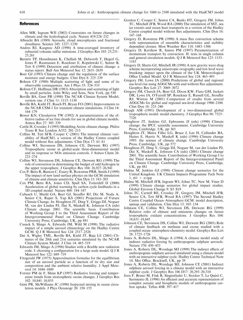
References

Allen MR, Ingram WJI (2002) Constraints on future changes inclimate and the hydrological cycle. Nature 419:224–232

Albrecht BA (1989) Aerosols, cloud microphysics and fractionalcloudiness. Science 245: 1227–1230

Andres RJ, Kasgnoc AD (1998) A time-averaged inventory ofsubaerial volcanic sulfur emissions. J Geophys Res 103: 25,251–25,261

Barnett TP, Hasselmann K, Chelliah M, Delworth T, Hegerl G,Jones P, Rasmussen E, Roeckner E, Ropelewski C, Santer B,Tett S (1999) Detection and attribution of climate change: astatus report. Bull Am Meteorol Soc 12: 2631–2659

Boer GJ (1993) Climate change and the regulation of the surfacemoisture and energy budgets. Clim Dyn 8: 225–239

Bohren CF (1980) Multiple scattering of light and some of itsobservable consequences. Am J Phys 55: 524–533

Bohren CF, Huffman DR (1983) Absorption and scattering of lightby small particles. John Wiley and Sons, New York, pp 530

Boville BA, Gent PR (1998) The NCAR Climate System Model,version one. J Clim 11: 1115–1130

Boville BA, Kiehl JT, Rasch PJ, Bryan FO (2001) Improvements tothe NCAR CSM-1 for transient climate simulations. J Clim 14:164–179

Bower KN, Choularton TW (1992) A parametrization of the ef-fective radius of ice free clouds for use in global climate models.Atmos Res 27: 305–339

Cattle H, Crossley J (1995) Modelling Arctic climate change. PhilosTrans R Soc London A352: 201–213

Collins M, Tett SFB, Cooper C (2001) The internal climate vari-ability of HadCM3, a version of the Hadley Centre coupledmodel without flux adjustments. Clim Dyn 17: 61–81

Collins WJ, Stevenson DS, Johnson CE, Derwent RG (1997)Tropospheric ozone in global-scale three-dimensional modeland its response to NOx emission controls. J Atmos Chem 26:223–274

Collins WJ, Stevenson DS, Johnson CE, Derwent RG (1999) Therole of convection in determining the budget of odd hydrogen inthe upper troposphere. J Geophys Res 104: 26,927–26,941

Cox P, Betts R, Bunton C, Essery R, Rowntree PRR, Smith J (1999)The impact of new land surface physics on the GCM simulationof climate and climate sensitivity. Clim Dyn 15: 183–203

Cox PM, Betts RA, Jones CD, Spall SA, Totterdell IJ (2000)Acceleration of global warming by carbon cycle feedbacks in a3D coupled model. Nature 408: 184–187

Cubasch U, Meehl GA, Boer GJ, Stouffer RJ, Dix M, Noda A,Senior CA, Raper S, Yap KS (2001) Projections of FutureClimate Change. In: Houghton JT, Ding Y, Griggs DJ, NoguerM, van der Linden PJ, Dai X, Maskell K, Johnson CA (eds)Climate change 2001. The scientific basis. Contributionof Working Group I to the Third Assessment Report of theIntergovernmental Panel on Climate Change. CambridgeUniversity Press, Cambridge, UK, pp 881

Cusack S, Slingo A, Edwards JM, Wild M (1998) The radiativeimpact of a simple aerosol climatology on the Hadley CentreGCM. Q J R Meteorol Soc 124: 2517–2526

Dai A, Wigley TML, Boville BA, Kiehl JT, Buja LE (2001) Cli-mates of the 20th and 21st centuries simulated by the NCARClimate System Model. J Clim 14: 485–519

Edwards JM, Slingo A (1996) Studies with a flexible new radiationcode. I: choosing a configuration for a large scale model. Q J RMeteorol Soc 122: 689–719

Fitzgerald JW (1975) Approximation formulas for the equilibriumsize of an aerosol particle as a function of its dry size andcomposition and the ambient relative humidity. J Appl Mete-orol 14: 1044–1049

Forster PM de F, Shine KP (1997) Radiative forcing and temper-ature trends from stratospheric ozone changes. J Geophys Res102: 10,841–10,855

Gent PR, McWilliams JC (1990) Isopycnal mixing in ocean circu-lation models. J Phys Oceanogr 20: 150–155

Gordon C, Cooper C, Senior CA, Banks HT, Gregory JM, JohnsTC, Mitchell JFB, Wood RA (2000) The simulation of SST, seaice extents and ocean heat transports in a version of the HadleyCentre coupled model without flux adjustments. Clim Dyn 16:147–168

Gregory D, Rowntree PR (1990) A mass flux convection schemewith representation of ensemble characteristics and stabilitydependent closure. Mon Weather Rev 118: 1483–1506

Gregory D, Kershaw R, Inness PM (1997) Parametrization ofmomentum transport by convection. II: tests in single columnand general circulation models. Q J R Meteorol Soc 123: 1153–1183

Gregory D, Shutts GJ, Mitchell JR (1998) A new gravity wave dragscheme incorporating anisotropic orography and low level wavebreaking: impact upon the climate of the UK MeteorologicalOffice Unified Model. Q J R Meteorol Soc 124: 463–493

Gregory JM, Lowe JA (2000) Predictions of global and regionalsea-level rise using AOGCMs with and without flux adjustment.Geophys Res Lett 27: 3069–3072

Gregory JM, Church JA, Boer GJ, Dixon KW, Flato GM, JackettDR, Lowe JA, O’Farrell SP, Roeckner E, Russell GL, StoufferRJ, Winton M (2001) Comparison of results from severalAOGCMs for global and regional sea-level change 1900–2100.Clim Dyn 18: 225–240

Hough AM (1991) Development of a two-dimensional globaltropospheric model: model chemistry. J Geophys Res 96: 7325–7326

Houghton JT, Jenkins GJ, Ephraums JJ (eds) (1990) Climatechange: the IPCC scientific assessment. Cambridge UniversityPress, Cambridge, UK, pp 365

Houghton JT, Meira Filho LG, Bruce J, Lee H, Callander BA,Haites E, Harris N, Maskell K (eds) (1996) Climate change1995: the science of climate change. Cambridge UniversityPress, Cambridge, UK, pp 572

Houghton JT, Ding Y, Griggs DJ, Noguer M, van der Linden PJ,Dai X, Maskell K, Johnson CA (eds) (2001) Climate change2001. The scientific basis. Contribution of Working Group I tothe Third Assessment Report of the Intergovernmental Panelon Climate Change. Cambridge University Press, Cambridge,UK, pp 881

Hulme M, Jenkins GJ (1998) Climate change scenarios for theUnited Kingdom. UK Climate Impacts Programme Tech Note1, (61 + xv)pp

Hulme M, Mitchell JFB, Ingram WJ, Johns TC, New M, Viner D(1999) Climate change scenarios for global impact studies.Global Environ Change 9: S3–S19

Johns TC, Carnell RE, Crossley JF, Gregory JM, Mitchell JFB,Senior CA, Tett SFB, Wood RA (1997) The Second HadleyCentre Coupled Ocean–Atmosphere GCM: model description,spinup and validation. Clim Dyn 13: 103–134

Johnson CE, Collins WJ, Stevenson DS, Derwent RG (1999)Relative roles of climate and emissions changes on futuretropospheric oxidant concentrations. J Geophys Res 104:18,631–18,645

Johnson CE, Stevenson DS, Collins WJ, Derwent RG (2001) Roleof climate feedback on methane and ozone studied with acoupled ocean–atmosphere-chemistry model. Geophys Res Lett28: 1723–1726

Jones A, Roberts DL, Slingo A (1994) A climate model study ofindirect radiative forcing by anthropogenic sulphate aerosols.Nature 370: 450–453

Jones A, Roberts DL, Woodage MJ (1999) The indirect effects ofanthropogenic sulphate aerosol simulated using a climate modelwith an interactive sulphur cycle. Hadley Centre Technical Note14, Met Office, Bracknell, UK, pp 39

Jones A, Roberts DL, Woodage MJ, Johnson CE (2001) Indirectsulphate aerosol forcing in a climate model with an interactivesulphur cycle. J Geophys Res 106 D17: 20,293–20,310

Joos F, Bruno M, Fink R, Siegenthaler U, Stocker T, Le Quere C,Sarmiento JL (1996) An efficient and accurate representation ofcomplex oceanic and biospheric models of anthropogenic car-bon uptake. Tellus 48B: 397–417


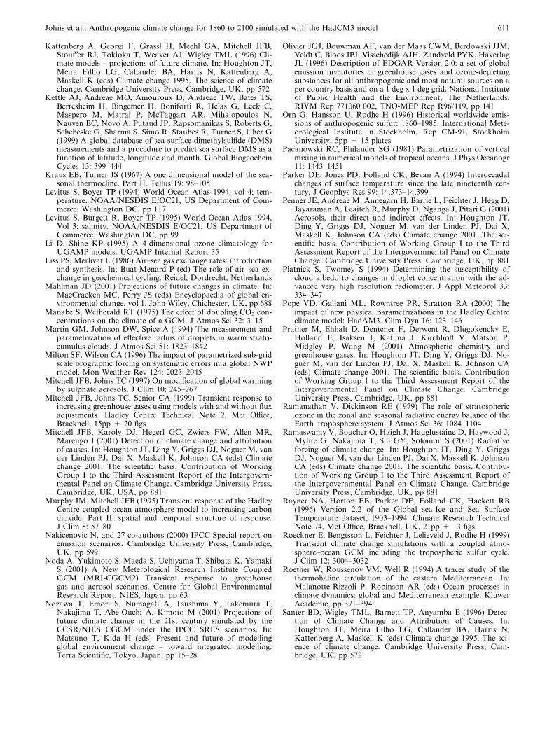
Kattenberg A, Georgi F, Grassl H, Meehl GA, Mitchell JFB,Stouffer RJ, Tokioka T, Weaver AJ, Wigley TML (1996) Cli-mate models – projections of future climate. In: Houghton JT,Meira Filho LG, Callander BA, Harris N, Kattenberg A,Maskell K (eds) Climate change 1995. The science of climatechange. Cambridge University Press, Cambridge, UK, pp 572

Kettle AJ, Andreae MO, Amouroux D, Andreae TW, Bates TS,Berresheim H, Bingemer H, Boniforti R, Helas G, Leck C,Maspero M, Matrai P, McTaggart AR, Mihalopoulos N,Nguyen BC, Novo A, Putaud JP, Rapsomanikas S, Roberts G,Schebeske G, Sharma S, Simo R, Staubes R, Turner S, Uher G(1999) A global database of sea surface dimethylsulfide (DMS)measurements and a procedure to predict sea surface DMS as afunction of latitude, longitude and month. Global BiogeochemCycles 13: 399–444

Kraus EB, Turner JS (1967) A one dimensional model of the sea-sonal thermocline. Part II. Tellus 19: 98–105

Levitus S, Boyer TP (1994) World Ocean Atlas 1994, vol 4: tem-perature. NOAA/NESDIS E/OC21, US Department of Com-merce, Washington DC, pp 117

Levitus S, Burgett R, Boyer TP (1995) World Ocean Atlas 1994,Vol 3: salinity. NOAA/NESDIS E/OC21, US Department ofCommerce, Washington DC, pp 99

Li D, Shine KP (1995) A 4-dimensional ozone climatology forUGAMP models. UGAMP Internal Report 35

Liss PS, Merlivat L (1986) Air–sea gas exchange rates: introductionand synthesis. In: Buat-Menard P (ed) The role of air–sea ex-change in geochemical cycling. Reidel, Dordrecht, Netherlands

Mahlman JD (2001) Projections of future changes in climate. In:MacCracken MC, Perry JS (eds) Encyclopaedia of global en-vironmental change, vol 1. John Wiley, Chichester, UK, pp 688

Manabe S, Wetherald RT (1975) The effect of doubling CO2 con-centrations on the climate of a GCM. J Atmos Sci 32: 3–15

Martin GM, Johnson DW, Spice A (1994) The measurement andparametrization of effective radius of droplets in warm strato-cumulus clouds. J Atmos Sci 51: 1823–1842

Milton SF, Wilson CA (1996) The impact of parametrized sub-gridscale orographic forcing on systematic errors in a global NWPmodel. Mon Weather Rev 124: 2023–2045

Mitchell JFB, Johns TC (1997) On modification of global warmingby sulphate aerosols. J Clim 10: 245–267

Mitchell JFB, Johns TC, Senior CA (1999) Transient response toincreasing greenhouse gases using models with and without fluxadjustments. Hadley Centre Technical Note 2, Met Office,Bracknell, 15pp + 20 figs

Mitchell JFB, Karoly DJ, Hegerl GC, Zwiers FW, Allen MR,Marengo J (2001) Detection of climate change and attributionof causes. In: Houghton JT, Ding Y, Griggs DJ, Noguer M, vander Linden PJ, Dai X, Maskell K, Johnson CA (eds) Climatechange 2001. The scientific basis. Contribution of WorkingGroup I to the Third Assessment Report of the Intergovern-mental Panel on Climate Change. Cambridge University Press,Cambridge, UK, USA, pp 881

Murphy JM, Mitchell JFB (1995) Transient response of the HadleyCentre coupled ocean atmosphere model to increasing carbondioxide. Part II: spatial and temporal structure of response.J Clim 8: 57–80

Nakicenovic N, and 27 co-authors (2000) IPCC Special report onemission scenarios. Cambridge University Press, Cambridge,UK, pp 599

Noda A, Yukimoto S, Maeda S, Uchiyama T, Shibata K, YamakiS (2001) A New Meterological Research Institute CoupledGCM (MRI-CGCM2) Transient response to greenhousegas and aerosol scenarios. Centre for Global EnvironmentalResearch Report, NIES, Japan, pp 63

Nozawa T, Emori S, Numagati A, Tsushima Y, Takemura T,Nakajima T, Abe-Ouchi A, Kimoto M (2001) Projections offuture climate change in the 21st century simulated by theCCSR/NIES CGCM under the IPCC SRES scenarios. In:Matsuno T, Kida H (eds) Present and future of modellingglobal environment change – toward integrated modelling.Terra Scientific, Tokyo, Japan, pp 15–28

Olivier JGJ, Bouwman AF, van der Maas CWM, Berdowski JJM,Veldt C, Bloos JPJ, Visschedijk AJH, Zandveld PYK, HaverlagJL (1996) Description of EDGAR Version 2.0: a set of globalemission inventories of greenhouse gases and ozone-depletingsubstances for all anthropogenic and most natural sources on aper country basis and on a 1 deg x 1 deg grid. National Instituteof Public Health and the Environment, The Netherlands.RIVM Rep 771060 002, TNO-MEP Rep R96/119, pp 141

Orn G, Hansson U, Rodhe H (1996) Historical worldwide emis-sions of anthropogenic sulfur: 1860–1985. International Mete-orological Institute in Stockholm, Rep CM-91, StockholmUniversity, 5pp + 15 plates

Pacanowski RC, Philander SG (1981) Parametrization of verticalmixing in numerical models of tropical oceans. J Phys Oceanogr11: 1443–1451

Parker DE, Jones PD, Folland CK, Bevan A (1994) Interdecadalchanges of surface temperature since the late nineteenth cen-tury, J Geophys Res 99: 14,373–14,399

Penner JE, Andreae M, Annegarn H, Barrie L, Feichter J, Hegg D,Jayaraman A, Leaitch R, Murphy D, Nganga J, Pitari G (2001)Aerosols, their direct and indirect effects. In: Houghton JT,Ding Y, Griggs DJ, Noguer M, van der Linden PJ, Dai X,Maskell K, Johnson CA (eds) Climate change 2001. The sci-entific basis. Contribution of Working Group I to the ThirdAssessment Report of the Intergovernmental Panel on ClimateChange. Cambridge University Press, Cambridge, UK, pp 881

Platnick S, Twomey S (1994) Determining the susceptibility ofcloud albedo to changes in droplet concentration with the ad-vanced very high resolution radiometer. J Appl Meteorol 33:334–347

Pope VD, Gallani ML, Rowntree PR, Stratton RA (2000) Theimpact of new physical parametrizations in the Hadley Centreclimate model: HadAM3. Clim Dyn 16: 123–146

Prather M, Ehhalt D, Dentener F, Derwent R, Dlugokencky E,Holland E, Isaksen I, Katima J, Kirchhoff V, Matson P,Midgley P, Wang M (2001) Atmospheric chemistry andgreenhouse gases. In: Houghton JT, Ding Y, Griggs DJ, No-guer M, van der Linden PJ, Dai X, Maskell K, Johnson CA(eds) Climate change 2001. The scientific basis. Contributionof Working Group I to the Third Assessment Report of theIntergovernmental Panel on Climate Change. CambridgeUniversity Press, Cambridge, UK, pp 881

Ramanathan V, Dickinson RE (1979) The role of stratosphericozone in the zonal and seasonal radiative energy balance of theEarth–troposphere system. J Atmos Sci 36: 1084–1104

Ramaswamy V, Boucher O, Haigh J, Hauglustaine D, Haywood J,Myhre G, Nakajima T, Shi GY, Solomon S (2001) Radiativeforcing of climate change. In: Houghton JT, Ding Y, GriggsDJ, Noguer M, van der Linden PJ, Dai X, Maskell K, JohnsonCA (eds) Climate change 2001. The scientific basis. Contribu-tion of Working Group I to the Third Assessment Report ofthe Intergovernmental Panel on Climate Change. CambridgeUniversity Press, Cambridge, UK, pp 881

Rayner NA, Horton EB, Parker DE, Folland CK, Hackett RB(1996) Version 2.2 of the Global sea-Ice and Sea SurfaceTemperature dataset, 1903–1994. Climate Research TechnicalNote 74, Met Office, Bracknell, UK, 21pp + 13 figs

Roeckner E, Bengtsson L, Feichter J, Lelieveld J, Rodhe H (1999)Transient climate change simulations with a coupled atmo-sphere–ocean GCM including the tropospheric sulfur cycle.J Clim 12: 3004–3032

Roether W, Roussenov VM, Well R (1994) A tracer study of thethermohaline circulation of the eastern Mediterranean. In:Malanotte-Rizzoli P, Robinson AR (eds) Ocean processes inclimate dynamics: global and Mediterranean example. KluwerAcademic, pp 371–394

Santer BD, Wigley TML, Barnett TP, Anyamba E (1996) Detec-tion of Climate Change and Attribution of Causes. In:Houghton JT, Meira Filho LG, Callander BA, Harris N,Kattenberg A, Maskell K (eds) Climate change 1995. The sci-ence of climate change. Cambridge University Press, Cam-bridge, UK, pp 572


Schimel D, and 26 co-authors (1996) Radiative forcing of climatechange. In: Houghton JT, Meira Filho LG, Callander BA,Harris N, Kattenberg A, Maskell K (eds) Climate change 1995.The science of climate change. Cambridge University Press,Cambridge, UK, pp 572

Shine KP, Derwent RG, Wuebbles DJ, Morcrette J-J (1990) Ra-diative forcing of climate. In: Houghton JT, Jenkins GJ,Ephraums JJ (eds) Climate change. The IPCC scientific as-sessment. Cambridge University Press, Cambridge, UK, pp 365

Smith RNB (1990) A scheme for predicting layer clouds and theirwater content in a general circulation model. Q J R MeteorolSoc 116: 435–460

Stendel M, Schmith T, Roeckner E, Cubasch U (2000) The climateof the 21st century: transient simulations with a coupled at-mosphere–ocean general circulation model. Danmarks Klima-center Report 00-6, Danish Meteorological Institute,Copenhagen, Denmark, pp 51

Stevenson DS, Johnson CE, Collins WJ, Derwent RG, EdwardsJM (2000) Future estimates of tropospheric ozone radiativeforcing and methane turnover – the impact of climate change.Geophys Res Lett 27: 2073–2076

Stott PA, Tett SFB, Jones GS, Allen MR, Ingram WJ, MitchellJFB (2001) Attribution of twentieth century temperaturechange to natural and anthropogenic causes. Clim Dyn 17: 1–21

Tett SFB, Stott PA, Allen MR, Ingram WJ, Mitchell JFB (1999)Causes of twentieth century temperature change. Nature 399:569–572

Tett SFB, Jones GS, Stott PA, Hill D, Mitchell JFB, Allen MR,Ingram WJ, Johns TC, Johnson CE, Jones A, Roberts DL,Sexton DMH, Woodage MJ (2002) Estimation of natural andanthropogenic contributions to 20th century climate tempera-ture change. J Geophys Res 107 (D16), 10.1029/2000JD000028

Toon OB, Pollack JB, Khare BN (1976) The optical constants ofseveral atmospheric aerosol species: ammonium sulfate, alu-minium oxide, and sodium chloride. J Geophys Res 81: 5733–5748

US National Assessment synthesis team (2000) Climate changeimpacts on the United States. US Global Change Programme,Cambridge University Press, pp 154

Visbeck M, Marshall J, Haine T, Spall M (1997) On the specifi-cation of eddy transfer coefficients in coarse resolution oceancirculation models. J Phys Oceanogr 27: 381–402

Wang HJ, Cunnold DM, Bao X (1996) A critical analysis ofstratospheric aerosol and gas experiment ozone trends. J Geo-phys Res 101 D7: 12,495–12,514

Williams KD, Senior CA, Mitchell JFB (2001a) Transient climatechange in the Hadley Centre models: the role of physical pro-cesses. J Clim 14: 2659–2674

Williams KD, Jones A, Roberts DL, Senior CA, Woodage MJ(2001b) The response of the climate system to the indirect ef-fects of anthropogenic sulfate aerosol. Clim Dyn 17: 845–856

Wood RA, Keen AB, Mitchell JFB, Gregory JM (1999) Changingspatial structure of the thermohaline circulation in response toatmospheric CO2 forcing in a climate model. Nature 399: 572–575

Woodward S (2001) Modelling the atmospheric life cycle and ra-diative impact of mineral dust in the Hadley Centre climatemodel. J Geophys Res 106: 18,155–18,166

Wright DK (1997) A new eddy mixing parametrization and oceangeneral circulation model. International WOCE News 26: 27–29

Xie P, Arkin PA (1997) Global precipitation: a 17-year monthlyanalysis based on gauge observations, satellite estimates andnumerical model outputs. Bull Am Meteorol Soc 78: 2539–2558


Anthropogenic climate change for 1860 to 2100 simulated with the HadCM3 model under updated...

Documents

Transcript of Anthropogenic climate change for 1860 to 2100 simulated with the HadCM3 model under updated...