
Modeling Multilevel Supply Chain Systems to Optimize Order ...
210
Old Dominion University Old Dominion University ODU Digital Commons ODU Digital Commons Mechanical & Aerospace Engineering Theses & Dissertations Mechanical & Aerospace Engineering Spring 2005 Modeling Multilevel Supply Chain Systems to Optimize Order Modeling Multilevel Supply Chain Systems to Optimize Order Quantities and Order Points Through Mathematical Models, Quantities and Order Points Through Mathematical Models, Discrete Event simulation and Physical Simulations Discrete Event simulation and Physical Simulations Alok K. Verma Old Dominion University Follow this and additional works at: https://digitalcommons.odu.edu/mae_etds Part of the Industrial Engineering Commons, and the Mechanical Engineering Commons Recommended Citation Recommended Citation Verma, Alok K.. "Modeling Multilevel Supply Chain Systems to Optimize Order Quantities and Order Points Through Mathematical Models, Discrete Event simulation and Physical Simulations" (2005). Doctor of Philosophy (PhD), Dissertation, Mechanical & Aerospace Engineering, Old Dominion University, DOI: 10.25777/80t1-2z36 https://digitalcommons.odu.edu/mae_etds/162 This Dissertation is brought to you for free and open access by the Mechanical & Aerospace Engineering at ODU Digital Commons. It has been accepted for inclusion in Mechanical & Aerospace Engineering Theses & Dissertations by an authorized administrator of ODU Digital Commons. For more information, please contact [email protected].
-
Upload
khangminh22 -
Category
Documents
-
view
4 -
download
0
Transcript of Modeling Multilevel Supply Chain Systems to Optimize Order ...

Old Dominion University Old Dominion University
ODU Digital Commons ODU Digital Commons
Mechanical & Aerospace Engineering Theses & Dissertations Mechanical & Aerospace Engineering
Spring 2005
Modeling Multilevel Supply Chain Systems to Optimize Order Modeling Multilevel Supply Chain Systems to Optimize Order
Quantities and Order Points Through Mathematical Models, Quantities and Order Points Through Mathematical Models,
Discrete Event simulation and Physical Simulations Discrete Event simulation and Physical Simulations
Alok K. Verma Old Dominion University
Follow this and additional works at: https://digitalcommons.odu.edu/mae_etds
Part of the Industrial Engineering Commons, and the Mechanical Engineering Commons
Recommended Citation Recommended Citation Verma, Alok K.. "Modeling Multilevel Supply Chain Systems to Optimize Order Quantities and Order Points Through Mathematical Models, Discrete Event simulation and Physical Simulations" (2005). Doctor of Philosophy (PhD), Dissertation, Mechanical & Aerospace Engineering, Old Dominion University, DOI: 10.25777/80t1-2z36 https://digitalcommons.odu.edu/mae_etds/162
This Dissertation is brought to you for free and open access by the Mechanical & Aerospace Engineering at ODU Digital Commons. It has been accepted for inclusion in Mechanical & Aerospace Engineering Theses & Dissertations by an authorized administrator of ODU Digital Commons. For more information, please contact [email protected].

MODELING MULTILEVEL SUPPLY CHAIM SYSTEMS TO
OPTIMIZE ORDER QUANTITIES AND ORDER POINTS
THROUGH MATHEMATICAL MODELS, DISCRETE EVENT
SIMULATION AND PHYSICAL SIMULATIONS
by
Alok K. VermaB. Sc. December 1978, Indian Institute of Technology, Kanpur
M.E. August 1981, Old Dominion University
A Dissertation Submitted to the Faculty of Old Dominion University in Partial Fulfillment of the
Requirements for the Degree of
DOCTOR OF PHILOSOPHY
m
MECHANICAL ENGINEERING
OLD DOMINION UNIVERSITY May 2005
Approved by:
Han P. or)
Moo! Gupta (Member)
Gene Hou (Member)
Resit l/uoi \ivxuuj.uvi f
Reproduced with permission of the copyright owner. Further reproduction prohibited without permission.
ABSTRACT
MODELING MULTILEVEL SUPPLY CHAIN SYSTEMS TO OPTIMIZE ORDER
QUANTITIES AND ORDER POINTS THROUGH MATHEMATICAL MODELS,
DISCRETE EVENT SIMULATION AND PHYSICAL SIMULATIONS
Alok K. Verma Old Dominion University, 2005
Director: Dr. Han P. Bao
Managing supply chains in today’s distributed manufacturing environment has
become more complex. To remain competitive in today’s global marketplace,
organizations must streamline their supply chains. The practice of coordinating the
design, procurement, flow of goods, services, information and finances, from raw
material flows to parts supplier to manufacturer to distributor to retailer and finally to
consumer requires synchronized planning and execution. Efficient and effective supply
chain management assists an organization in getting the right goods and services to the
place needed at the right time, in the proper quantity and at acceptable cost. Managing
this process involves developing and overseeing relationships with suppliers and
customers, controlling inventory, and forecasting demand, all requiring constant feedback
from every link in the chain. Base Stock Model and (Q, r) models are applied to three tier
single-product supply chain to calculate order quantities and reorder point at various
locations within the supply chain. Two physical simulations are designed to study the
above supply chain. One of these simulations is specifically designed to validate the
results from Base Stock model. A computer based discrete event simulation model is
created to study the three tier supply chain and to validate the results of the Base Stock
model. Results from these mathematical models, physical simulation models and
computer based simulation model are compared. In addition, the physical simulation
model studies the impact of lean implementation through various performance metrics
and the results demonstrate the power of physical simulations as a pedagogical tool for
training. Contribution of present work in understanding the supply chain integration is
discussed and future research topics are presented.
Reproduced with permission of the copyright owner. Further reproduction prohibited without permission.

In loving memory of my late mother
Mrs. Kamala Devi
for her selfless and dedicated service to our family.
With respect and gratitude to my father
Mr. I. P. Verma
for his support and guidance
Reproduced with permission of the copyright owner. Further reproduction prohibited without permission.

ACKNOWLEDGMENTS
I would like to express my sincere appreciation to Drs Han Bao and Resit Unal
without whom, this work would not be possible. Thanks to Dr. Bao for being a guiding
light and directing this research effort towards a successful completion. I am indebted to
Drs Mool Gupta and Gene Hon for serving on the dissertation committee and to Dr.
Suren Dwivedi for always encouraging me to complete my PhD work. Additional thanks
are due to Dean Oktay Baysal, Professor Emeritus William D. Stanley, Professor Gary
Crossman and Dr. Paul Kauffman for their valuable support and encouragement.
I would like to express my gratitude to Northrop Grumman Newport News
(NGNN) for supporting my initial work in the area of Lean Manufacturing and for
providing me an industry perspective. Sincere thanks are due to Dr. James Hughes, Mr,
Robert Leber and Mr. William McHenry of NGNN. Bill and I have spent countless hours
working together on the Lean Enterprise Simulation Project. My sincere gratitude to
National Shipbuilding Research Program (NSRP) for supporting the work on simulation
development.
Finally this work would not be possible without the support from my family.
Through all these years, my wife Rashmi, was supportive of my endeavor and took care
of all responsibilities including, taking care of our children and thus allowing me to focus
on my research. I am grateful to my children Shalini and Shivesh for their understanding
of my absence. Sincere appreciation to my parents in-law Dr Ram Chandra Gupta and
Mrs. Bimla Gupta, my uncle Dr. D. K. Singh and, my brother Prof. V.K. Verma for their
persistent encouragement and support. Drs Ram Bachan Ram, Sudhir Mehrotra, Rahul
Gupta. K. P. Singh, Satyajit Verma and Aran Verma were also constant source of
encouragement. Thanks to Amol Sonje for helping me run various cases of mathematical
models and to Harsh for his help with supply chain simulation development. Thanks to
Tiffany Brittingham and Diane Mitchell for providing help with formatting the
manuscript.
Reproduced with permission of the copyright owner. Further reproduction prohibited without permission.

STABLE O F CONTENTS
Page
ABSTRACT............... ..... ........................ ii
DEDICATION............................................................................ iil
ACKNOWLEDGEMENTS....................................................................................................iv
TABLE OF CONTENTS .............. vi
LIST OF FIGURES ....... ix
LIST OF TABLES................. xi
CHAPTERS
1. Introduction..................................... ...1
2. Background Information...................................... 42.1. Lean Philosophy.................................................. ...42.2. Lean Enterprise............................................ .62.3. Value Streams and Supply Chains.......................... 72.4. Lean Extended Enterprise ............................. .....9
3. Supply Chain and its Management ....... ....103.1. Issues in Supply Chain Management................. 103.2. Basic Components of Supply Chain............................... 103.3. Lean Supply Chain Management.............................. ..................................123.4. Supply Chain Dynamics .......... ................................................143.5. Lean Buyer Supplier Relations......................................... 153.6. Reducing the Number of suppliers ..... 163.7. Four Levels of Buyer Supplier Relations .......... .............183.8. Lean Supplier Networks ......... ...........................................193.9. Performance Metrics in Supply Chain Management........................................203.10. Supply chain Management and Information Technology................. ..203.11 Reasons for Holding Inventory...................................................... ....223.12 Managing the Inventory....... ..... .......................................243.13 Managing Work in Progress ............................................................................263.14 Managing Finished Goods Inventory........................ 283.15 Managing Spare Parts ..... .............283.16 Multiechelon Supply Chains....................... .....................................................283.17 Flow in Supply Chains.....................................................................................31
a. Functional flows in Supply Chain...............................................................32b. Physical Flows in Supply Chain ....................33
Reproduced with permission of the copyright owner. Further reproduction prohibited without permission.
3.18 Summary...........................................................................................................37
4. Literature Survey .....................................384.1. Impact of ERP on Supply Chain Management.................................................384.2. Made to Store vs. Made to Order...... ..... ......394.3. How Gillette Cleaned its Supply Chain................... .......404.4. Bullwhip Effect.................................................................................................414.5. Managing Physical, Information and Financial Flows .....................................434.6. Supplier Relationship Management....... .... 444.7. Improving Extended Supply Chain Performance .... ...444.8. Supplier Development in Small & Medium Size Enterprise ...... 454.9. Information System Failure and its Impact.................... ...454.10 Implication of Postponement ..... 464.11 Very High Inventory ...... 464.12 Summary..... ..... ....474.13 Intent of Dissertation..................... .........48
5. Existing Mathematical Models............................................... 495.1. Deterministic Models ............. .......495.2. Stochastic Models .... 505.3. Base Stock Model.............. 515.4. Application of Base Stock - An Example.......................................... 555.5. The (Q, r) Model .................. ....575.6. Application of (Q, r) Model - An Example ...... 675.7 Summary ...... ..69
6. Application of Base Stock Model.... ..... ............................716.1. Replenishment Lead Time 12 Months ..... 736.2. Replenishment Lead Time 8 Months ..... 776.3. Replenishment Lead Time 6 M onths ........ 816.4. Replenishment Lead Time 4 Months ..... ................................846.5. Replenishment Lead Time 2 Months ................................................................886.6. Summary of Results for Base Stock Model ..... ..92
7. Application of (Q, r) Model................... ......................957.1. Replenishment Lead Time 12 M onths ...... .........977.2. Replenishment Lead Time 8 Months .... .........................................1047.3. Replenishment Lead Time 6 Months ..... 1087.4. Replenishment Lead Time 4 Months ... ........ .......1147.5. Replenishment Lead Time 2 Months .... ...........................1207.6. Summary Results for (Q, r) M odel.................................................................126
8. Physical Simulation of Base Stock Model................... .......................................1308.1. Goals of Physical Simulation.......................................................................... 1308.2. Simulation Activity.........................................................................................130
Reproduced with permission of the copyright owner. Further reproduction prohibited without permission.
viii
8.3. Simulation Layout...........................................................................................1308.4. Departments.... ...... .....1318.5. Simulation Activity Time Frame .......................................................1328.6. Phase-!................1... ....... 1338.7. Pfaase-II ..... ..............................................1338.8. Phase-Ill ..... .....................................................................................1348.9. Distribution of Demand ..................................................................................1348.10 Performance Metrics .....................................................................................1358.11 Summary..................... .................................1368.12 Forms Used ..... ........137
9. Physical Simulation of Supply Chain with Lean Principles .... 1409.1. Goals of Physical Simulation .......... ............1409.2. Introduction.... ............... 1409.3. Important Issues.. ..... .1419.4. Simulation Activity............... ............................1419.5. Model for Simulation .................... 1459.6. Implementation of Simulation Activity ........... 1469.7. Performance Metrics ..... ....1479.8. Summary ...... 148
10. Computer Based Simulation Model.......................... 15010.1 Goals of Computer Based Simulation ................ 15010.2 Software Used... ..... 15110.3 Simulation Layout............................................................ .15110.4 Simulation Results.............. 15210.5 Summary ..... ......158
11. Discussion on Results ...... 15912. Conclusions ........ 16213. Contributions of Present Research work. ..... 165
REFERENCES .......... 167
APPENDICESA Glossary of Lean Terms . ........ .................172B ProModel Simulation Program.................. 174C Author’s Publications ..... 177
VITA.. ...... ......198
Reproduced with permission of the copyright owner. Further reproduction prohibited without permission.
ix
LIST OF F lv JRES
Figure Page
1. New Structure of Today’s Supply Chain......................................................... ............2
2. Flow of Parts in a Two Tiered Supply Chain ...... ...........3
3. House of Lean and Tools ..... ...............5
4. Lean Enterprise.... ....... ....6
5. Intersecting and Merging Value Streams ...... 7
6. Value Stream for Cola Production.............. .......................... ..8
7. Lean Extended Enterprise ................. ...........9
8. Nature of Buyer-Supplier Relations......................................................... 16
9. Tiered Supply Chain..................................................................... 17
10. Lean Extended Enterprise..................... 21
11. Breakdown of WIP in Manufacturing Systems................ 23
12. Arborescent Multiechelon Supply Chains.................. 29
13. Variation in Demand at Different Levels of Supply Chain ........... ....31
14. Inventory vs. Time in (Q, r) Model.............. 58
15. Expected Inventory vs. Time in (Q, r) Model ............. .61
16. Base Stock Model Applied to Three level serial Supply Chain ......... 71
17. Total Cost vs. Replenishment Lead Time (Base Stock Model)................................93
18. Reorder Point vs. Replenishment Lead Time (Base Stock Model) ....... 94
19. (Q, r) Model Applied to Three Level Serial Supply Chain .................... .95
20. Cost vs. Replenishment Lead Time ((Q, r) model) ...... 128
21. Reorder Point vs. Replenishment Lead Time ((Q, r) model) ........ 129
22. Layout of Supply Chain for Physical Simulation...... ...... 131
23. Stat-Fit Screen Showing Poisson Distribution ...... .135
24. Parts Used in Simulation...... ...... .......137
25. Forms Used in Simulation... .......... .138
26. Forms Used in Simulation ..... .......139
27. Room Layout for Phase - I ....... ..141
Reproduced with permission of the copyright owner. Further reproduction prohibited without permission.
X
28. Variability Wheel ....................................................................................142
29. Room Layout for Phase-II .........................143
30. Communication through Three Phases.................... 143
31. Quality Check Wheel ..... 144
32. Room Layout for Phase -III.......................................................................... 144
33. Submarine Model Components................................................................................ 145
34. Submarine Aft Component ........... ........................145
35. Assembled Submarine Model.............................................. ...........................146
36. Performance Metrics Spreadsheet from Pilot Session ............148
37. Layout of the Supply Chain in ProModel....................... 152
38. Screen Display for Case with Zero Inventory Positions ..... .....................153
39. Screen Display for Case with Inventory Positions per Base Stock Model 154
40. Time Line for Various Variables................ ................156
41. Time Line for Various Variables ............ 156
42. State Chart for Locations............................ ................157
43. Percentage Utilization Chart..... ........... 157
44. Entity States of Engine and Engine Block...................... 158
Reproduced with permission of the copyright owner. Further reproduction prohibited without permission.

xi
LIST OF TABLES
'Table Page
1. Lean Benefits................................. ...............................................6
2. Issues in Supply Chain Management.................................................................. 10
3. Types of Network.. .... ....................19
4. Problems Faced by Gillette and Steps Taken......... ......................... ..41
5. Fill Rates for Various Values of r .................. ......56
6. p(r), G(r), n(r) Values for Various Values of r .......... ..................................... .68
7. Classification of Inventory Models ....................... ....70
8. Fill Rates for Various Values of r, 1 = 12 months ................ 74
9. Fill Rates for Various Values of r, 1 = 12 months.................. .............75
10. Fill Rates for Various Values of r, 1 = 12 months ........ 76
11. Fill Rates for Various Values of r, 1 = 8 months......................... 78
12. Fill Rates for Various Values of r, 1 = 8 months .......... 79
13. Fill Rates for Various Values of r, 1 = 8 months..................................................80
14. Fill Rates for Various Values of r, 1 = 6 months ..... 81
15. Fill Rates for Various Values ofr, 1 = 6 months ......... 82
16. Fill Rates for Various Values of r, 1 - 6 months.............. .....83
17. Fill Rates for Various Values of r, 1 = 4 months .....85
18. Fill Rates for Various Values ofr, 1 = 4 months........... ...................................86
19. Fill Rates for Various Values of r, 1 = 4 months ........ 87
20. Fill Rates for Various Values of r, 1 = 2 months ......... .....89
21. Fill Rates for Various Values of r, 1 = 2 months ..... 90
22. Fill Rates for Various Values ofr, 1 = 2 months ...... ......91
23. Summary of Application Runs of Base Stock Model.........................................92
24. Cost Results for Various Locations. ..... 93
25. p(r), G(r), n(r) Values for Various Values of r, 1 = 12 months ...........................98
26. p(r), G(r), n(r) Values for Various Values ofr, 1 = 12 months .........................100
27. p(r), G(r), n(r) Values for Various Values of r, 1 = 12 months ....... . 102
Reproduced with permission of the copyright owner. Further reproduction prohibited without permission.

xii
28. p(t), G(r), n(r) Values for Various Values of r, 1 = 8 months ........................... 105
29. p(r), G(r), n(r) Values for Various Values ofr, 1 = 8 months ..........106
30. p(r), G(r), n(r) Values for Various Values of r , ! = 6 months ........................... 109
31. p(r), G(r), n(r) Values for Various Values of r, 1 = 6 months ........ I l l
32. p(r), G(r), n(r) Values for Various Values of r, 1 = 6 months ...........................112
33. p(r), G(r), n(r) Values for Various Values ofr, 1 = 4 months .........115
34. p(r), G(r), n(r) Values for Various Values of r, 1 = 4 months ......... 116
35. p(r), G(r), n(r) Values for Various Values of r, 1 = 4 months ...... 118
36. p(r), G(r), n(r) Values for Various Values of r, 1 = 2 months .............. 121
37. p(r), G(r), n(r) Values for Various Values of r, 1 = 2 months ....... 122
38. p(r), G(r), n(r) Values for Various Values of r, 1 = 2 months ................. 124
39. Summary of Application Runs for (Q, r) Model............... 127
40. Cost Values for Various Replenishment Lead Time.......................... 127
41. Reorder Point for Various Replenishment Lead Time (Q, r) Model................ 128
42. Q for Various Replenishment Lead Times ........ 129
43. Order Quantity vs. Replenishment Lead Time......................... .............135
44. Performance Metric Spreadsheet....................... 136
45. Issues in Supply Chain and Lean Tools ....................... 141
46. Results from ProModel................................. 154
47. Locations and their State..................................................... .155
48. Multiple Capacity Locations and their State.................. 155
49. Variables Defined within the M odel ....... 155
Reproduced with permission of the copyright owner. Further reproduction prohibited without permission.

Chapter - 1
INTRODUCTION
Supply chain management is the integration of key business processes from end
user through suppliers and provides products, services, and information that add value for
customers and other stakeholders. In today’s highly competitive environment, companies
must manage costs if they are to survive. Cost management must be applied across the
entire life of the product by everyone involved in its design and manufacture. Cost
management cannot be limited to the four walls of a factory, it must spread across the
entire supply chain and cover all aspects of the value chain of the company’s products or
services.
However, it is more than just cost management that must extend across the
organizational boundaries between buyers and suppliers. Suppliers are major source of
innovation for lean enterprises [1] & [4], The key point is that the supply chain must be
managed for competitive advantage, not just to reduce cost. [13]
At the beginning of the Century, supply chains were paper chains, linearly
connecting manufacturers, warehouses, wholesalers, retailers and consumers. The chain
ranged from one or two to dozens of tiers and logistics were a nightmare. People and
paper physically connected various tiers together. Furthermore, the linear nature of the
chain made communication between the front-end and back-end of the chain messy and
time consuming.
The advent of Internet and computers has changed the structure of supply chain in
the later third of the 20th century. The following quote from the Stanford University web
site provides a glimpse of the new paradigm in supply chain and is illustrated in Figure 1.
“The latest generation o f supply chain management is Web-Centric. It is characterized
by the marriage o f the Internet and the supply chain and has resulted in the birth o f
electronic business (e-business) applications. These Internet enabled, e-business
Reproduced with permission of the copyright owner. Further reproduction prohibited without permission.
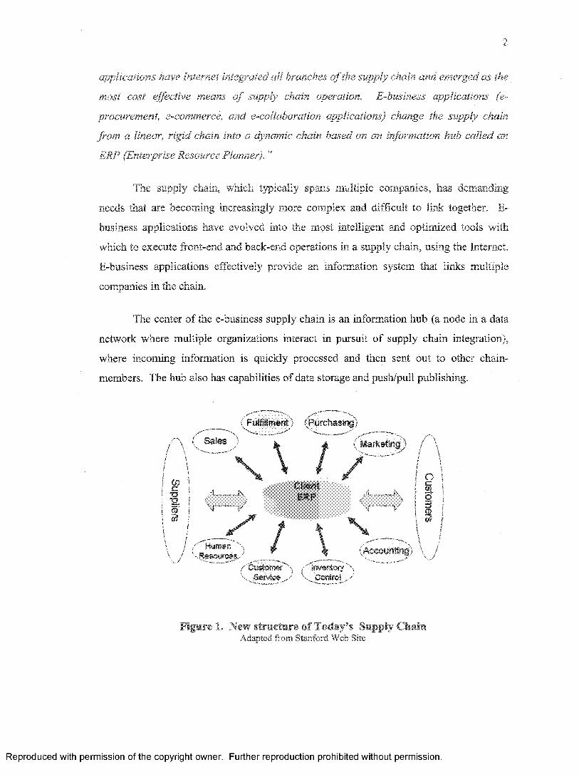
2
applications have Internet integrated all branches o f the supply chain and emerged as the
most cost effective means o f supply chain operation. E-business applications (e-
procurement, e-commerce, and e-collaboration applications) change the supply chain
from a linear, rigid chain into a dynamic chain based on an information hub called an
ERP (Enterprise Resource Planner). ”
The supply chain, which typically spans multiple companies, has demanding
needs that are becoming increasingly more complex and difficult to link together. E-
business applications have evolved into the most intelligent and optimized tools with
which to execute front-end and back-end operations in a supply chain, using the Internet.
E-business applications effectively provide an information system that links multiple
companies in the chain.
The center of the e-business supply chain is an information hub (a node in a data
network where multiple organizations interact in pursuit of supply chain integration),
where incoming information is quickly processed and then sent out to other chain-
members. The hub also has capabilities of data storage and push/pull publishing.
' F u l f i l l m e n t P u r c h a s i n g )
Sales ) i a ( Marketing) / \
„ ! I / ie“ , . Client . i SI i “ ! < 1.........i |I j ' ' " ' ( f r „ , * ( 1
Human / \Customer ''inventory y. Service J V Control
Figure 1. New structure of Today’s Supply ChainA dapted from Stanford W eb Site
Reproduced with permission of the copyright owner. Further reproduction prohibited without permission.
3
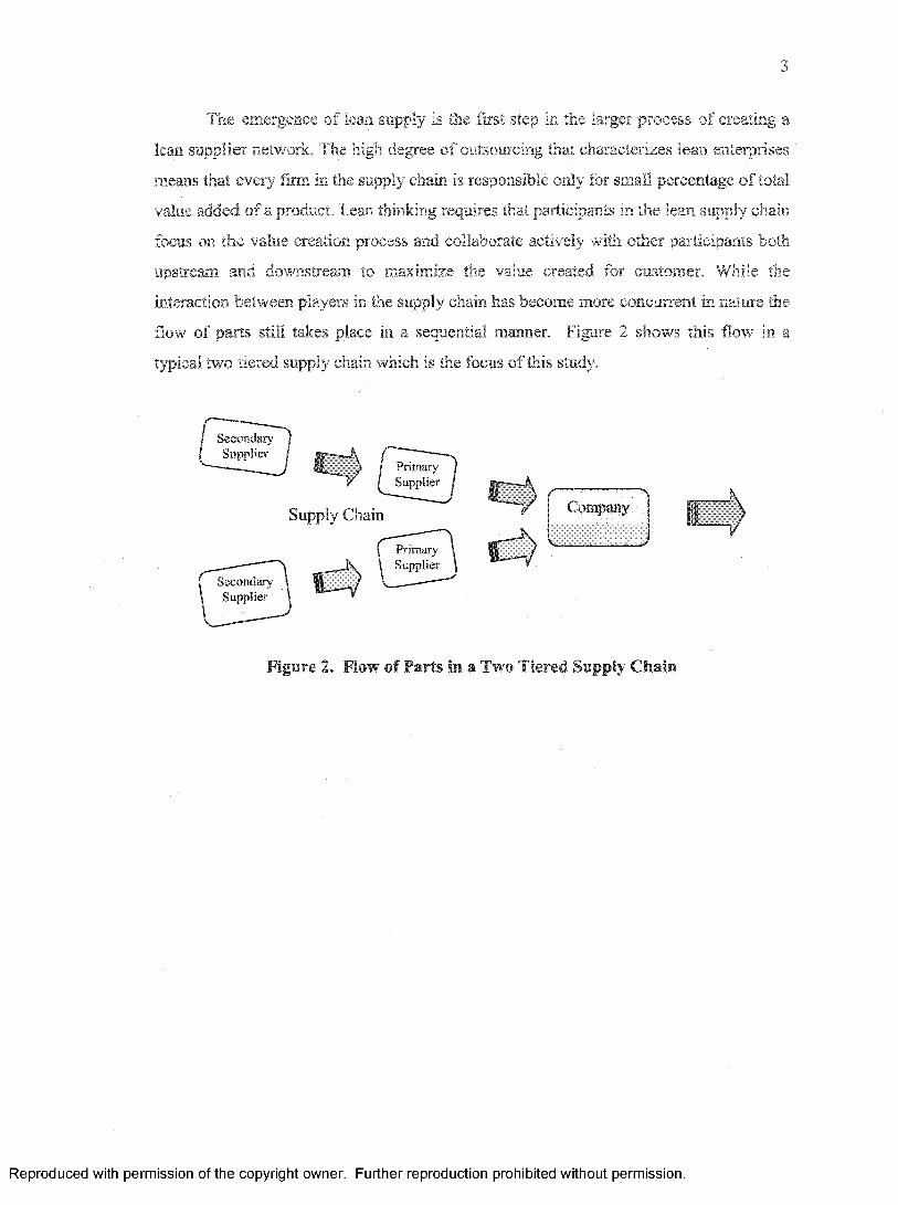
The emergence of lean supply is the first step in the larger process of creating a
lean supplier network. The high degree of outsourcing that characterizes lean enterprises
means that every firm in the supply chain is responsible only for small percentage of total
value added of a product. Lean thinking requires that participants in the lean supply chain
focus on the value creation process and collaborate actively with other participants both
upstream and downstream to maximize the value created for customer. While the
interaction between players in the supply chain has become more concurrent in nature the
flow of parts still takes place in a sequential manner. Figure 2 shows this flow in a
typical two tiered supply chain which is the focus of this study.
SecondarySupplier
PrimarySupplier
C om panySupply Chain
PrimarySupplier
SecondarySupplier
Figure 2. Flow of Parts in a Two Tiered Supply Chain
Reproduced with permission of the copyright owner. Further reproduction prohibited without permission.
4
Chapter — 2
BACKGROUND INFORMATION
2.1. Lean Philosophy
The term lean was first coined about 15 years ago at Massachusetts Institute of
Technology and later published in a book called Machine That Changed the World,
written by James Womack and his colleagues [4]. The generally accepted definition of
lean in the industrial community is that it is:
“A systematic approach to identifying and eliminating waste (non-value-added activities)
through continuous improvement by flowing the product at the pull o f the customer in
pursuit o f perfection.”
The lean principles have evolved from the works of Henry Ford and subsequent
development of Toyota Production System in Japan. Lean manufacturing principles
improve productivity by eliminating waste from the product’s value stream and by
making the product flow through the value stream without interruptions [1], [4] & [5].
This system in essence shifts the focus from individual machines and their utilization to
the flow of the product through processes [7].
Lean philosophy is people centric in the sense that it focuses on the value for the
customer and how this value can be increased by removing waste from the system and
increasing flow through the system by changing the way people think about their work. It
is more about people than the tools and techniques it employs. Lean defines value in
terms of the entire customer experience with the product [1]. A critical step in defining
value is the determination of target cost based upon the resources required to make a
product of given specification if all the muda (waste) was removed from the system.
In their book Lean Thinking, James Womack and Dan Jones [1] outline five steps
for implementing lean:
Reproduced with permission of the copyright owner. Further reproduction prohibited without permission.
5
!. Specify the value desired by the customer.
2. Identify the value stream for each product and challenge all waste.
3. Make the product flow through the value creating steps.
4. Introduce pull between all steps where continuous flow is possible.
5. Manage toward perfection by continuously improving the process.
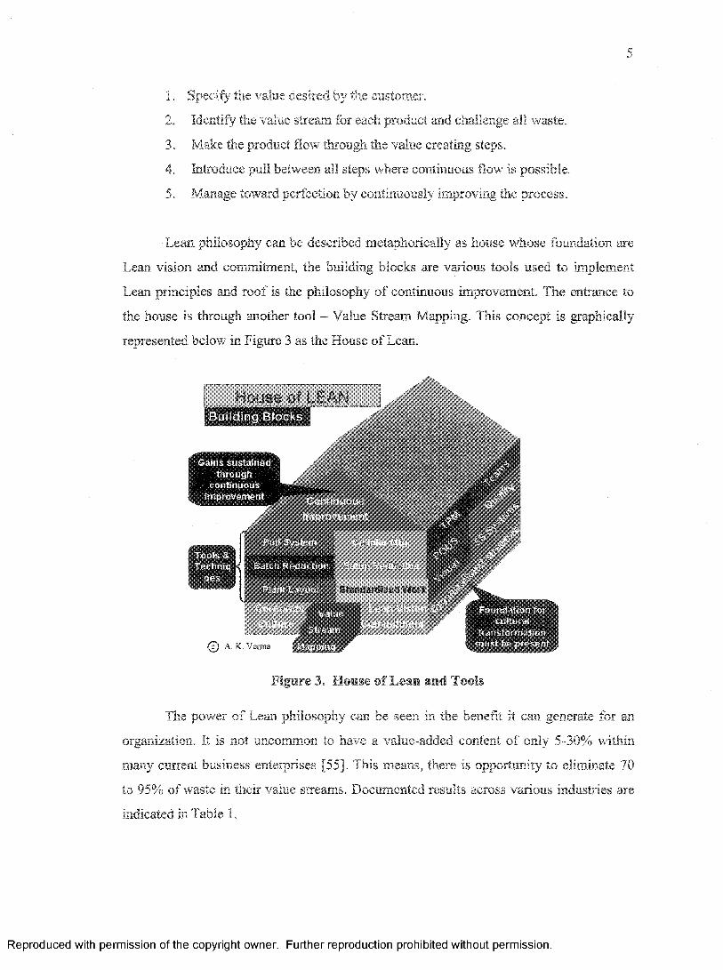
Lean philosophy can be described metaphorically as house whose foundation are
Lean vision and commitment, the building blocks are various tools used to implement
Lean principles and roof is the philosophy of continuous improvement. The entrance to
the house is through another tool - Value Stream Mapping. This concept is graphically
represented below in Figure 3 as the House of Lean.
House of LEANBuilding Blocks
mxmrmzed Worts
© A. K. Verma
Figure 3. House of Lean and Tools
The power of Lean philosophy can be seen in the benefit it can generate for an
organization. It is not uncommon to have a value-added content of only 5-30% within
many current business enterprises [55]. This means, there is opportunity to eliminate 70
to 95% of waste in their value streams. Documented results across various industries are
indicated in Table 1.
Reproduced with permission of the copyright owner. Further reproduction prohibited without permission.

6
Element BenefitCapacity Inventory Cycle Time Lead TimeProduct Development TimeSpaceFirst-pass Yield Service
10 to 20 % gain in capacity by optimizing bottlenecks Reduction of 30 to 40% in inventory Throughput time reduced by 50 to 75%Reduction of 50% in order fulfillment Reduction of 35 to 50% in development time 35 to 50% space reduction 5 to 15% increase in first-pass yield Delivery performance of 99%
TaMe 1. Lean Benefits
2.2. Lean Enterprise
When Lean principles are applied not just to manufacturing but to business
operations not only within the organization but across all supply chains, a lean enterprise
is created. Lean enterprise therefore is a set of synergistic processes along a value stream
to create value for the customer.
Human&
Capita!Resources
&
Resources
Raw Material
* \ Processes/3*
[ Compsny-A;
Production
Product
o\
Company-B
Physical Processes
Business Processes #A iokX . Vsrma
Figure 4. Lean Enterprise
Lean thinking encourages organizations to view itself as just one part of an
extended supply chain. It follows that organizations need to think strategically beyond
Reproduced with permission of the copyright owner. Further reproduction prohibited without permission.
7
their own. boundaries. Lean philosophy contends that because value streams flow across
several departments and functions within an organization, a company should be
organized around its key value streams. A value stream in general may cut across
organizational boundaries of several organizations as shown in Figure 4. Stretching
beyond the firm, some form of collective agreement or organization is needed to manage
the whole value stream for a product family, setting common improvement targets, rules
for sharing the gains and effort and for designing waste out of future product generations.
This collective group of organizations is called a lean enterprise.
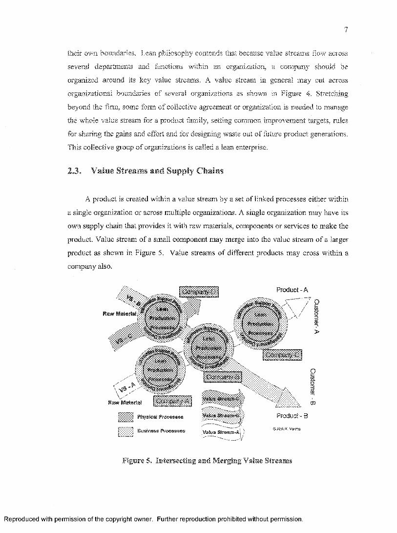
2.3. Value Streams and Supply Chains
A product is created within a value stream by a set of linked processes either within
a single organization or across multiple organizations. A single organization may have its
own supply chain that provides it with raw materials, components or services to make the
product. Value stream of a small component may merge into the value stream of a larger
product as shown in Figure 5. Value streams of different products may cross within a
company also.
Raw Material
Production
Comps
[com p an y-B
Raw Material
iCompany-D Product - A
Physical P rocesses Vsskws Stream-®’. ,
Business Processes•f -A \;¥aiue Stream-*! j
Figure 5. Intersecting and Merging Value Streams
Reproduced with permission of the copyright owner. Further reproduction prohibited without permission.
8
It is important to note that while the flow of parts and material may be linear
along a value stream, the flow- of information may be concurrent and may use an
Enterprise Resource Planning (ERP) system. This is further discussed in section 2.4 and
illustrated in Figure 7.
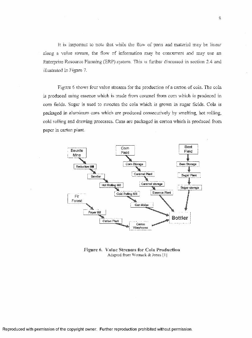
Figure 6 shows four value streams for the production of a carton of cola. The cola
is produced using essence which is made from caramel from com which is produced in
com fields. Sugar is used to sweeten the cola which is grown in sugar fields. Cola is
packaged in aluminum cans which are produced consecutively by smelting, hot rolling,
cold rolling and drawing processes. Cans are packaged in carton which is produced from
paper in carton plant.
BauxiteMine
X
ComField
XReduction I
| Com
BeetField
IBeet
Smelter " Caramel Plant Sugar Plant---- — ---- ...X... -... _ .........I......
Hot Rolling Mill Caramel storage W
■.......... ........ : | Sugar storage . I " .........'
i-orest
B e t te rCarton' Plant
CartonWarehouse
Figure 6. Value Streams for Cola ProductionAdapted from Womack & Jones [1]
Reproduced with permission of the copyright owner. Further reproduction prohibited without permission.

9
2.4, Lean Extended Enterprise
The highest generation of Lean is the Lean Extended Enterprise. Here, an
organization views all participating entities in the value stream (e.g., suppliers,
subcontractors, its own enterprise and customers) as part of its own. The Lean Extended
Enterprise is an expansion of the traditional notion of Lean to improve velocity,
flexibility, responsiveness, quality and cost across the entire value stream. The
effectiveness of each partner determines the effectiveness of entire value stream [55].
Supply Chain Management (SCM), Enterprise Resource Planning (ERP), Customer
Relations Management (CRM) and Suppliers Relations Management (SRM) and Product
Lifecycle Management (PLM) form an integral part of the Lean Extended Enterprise as
shown in Figure 7.
S u c p 'le r s
S'jr.Ciig'; : Relations
5L _ _
; ; jS y r. ain Va-'-agement ; ; j
■ :................H f 1j I p o p j ! ; R e la tio n s jj, : | | j Management] j j
. / ‘■■‘.Cl ;VE ‘ L
Lean Extended Enterprise j
Figure 7. Lean Extended EnterpriseAdapted from Burton & Boeder [55]
Reproduced with permission of the copyright owner. Further reproduction prohibited without permission.
10
Chapter - 3
SUPPLY CHAIN AND INVENTORY MANAGEMENT
3.1 Issues in Supply Chain Management
Traditional supply chains are plagued with inefficiencies resulting from
adversarial relationships among key players. These inefficiencies result in long lead time,
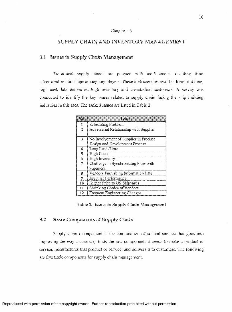
high cost, late deliveries, high inventory and un-satisfied customers. A survey was
conducted to identify the key issues related to supply chain facing the ship building
industries in this area. The ranked issues are listed in Table 2.
No, Issues1 Scheduling Problem2 Adversarial Relationship with Supplier
3 No Involvement of Supplier in Product Design and Development Process
4 Long Lead-Time5 High Costs6 High Inventory7 Challenge in Synchronizing Flow with
Suppliers.8 Vendors Furnishing Information Late9 Irregular Performance10 Higher Price to US Shipyards11 Shrinking Choice of Vendors12 Frequent Engineering Changes
Table 2. Issues in Supply Chain Management
3.2 Basic Components of Supply Chain
Supply chain management is the combination of art and science that goes into
improving the way a company finds the raw components it needs to make a product or
service, manufactures that product or service, and delivers it to customers. The following
are five basic components for supply chain management.
Reproduced with permission of the copyright owner. Further reproduction prohibited without permission.

1
a. Plan - This is the strategic portion of supply chain management. One needs a strategy
for managing all the resources that go toward meeting customer demand for one’s
product or sendee. A big piece of planning is developing a set of metrics to monitor the
supply chain so that it is efficient, costs less, and delivers high quality and value to
customers. Of many planning approaches that exist in business today, Management by
Planning (MBP) is unparalleled in its ability to articulate the objectives to be delivered,
the plans by which objectives will be delivered, the ownership of the team in delivering
the objectives, and management’s responsibility in aiding the team in meeting those
objectives. In Management by Objective (MBO), the stated objective becomes the focus
and not the process by which objective is achieved. By contrast, in Management by
Planning the goal is to become a learning organization through the activity of planning
and the implementation of theses plans [11]. Thus, MBP is a process oriented approach to
supply chain management.
Applying MBP to the integration of lean SCM and activities first involves
identifying common overarching objectives. Overarching objectives simply are the
highest level objectives based directly on strategic intent of the company.
b. Source - Choose the suppliers that will deliver the goods and services needed to create
product or service. Develop a set of pricing, delivery and payment processes with
suppliers and create metrics for monitoring and improving the relationships. And put
together processes for managing the inventory of goods and services received from
suppliers, including receiving shipments, verifying them, transferring them to
manufacturing facilities and authorizing supplier payments.
c. Make - This is the manufacturing step. Schedule the activities necessary for
production, testing, packaging and preparation for delivery. As the most metric-intensive
portion of the supply chain, measure quality levels, production output and worker
productivity.
d. Deliver - This is the part that many insiders refer to as "logistics." Logistic activities
include locating facilities, coordinating the receipt of orders from customers, developing
Reproduced with permission of the copyright owner. Further reproduction prohibited without permission.

12
a network o f warehouses, picking carriers to get products to customers and setting up an
invoicing system to receive payments etc. These activities have been integrated over the
past 50 years and are an essential function of supply chain management.
To achieve highest level of service at the lowest possible cost, it is necessary for
managers to examine the entire logistic system and not just one isolated facility or
activity such as transportation. The logistic system is concerned not only with the
physical placement of the facilities, but also with the levels of inventory and the flow of
material through those facilities [16]. Logistic includes the activities of sourcing and
purchasing, conversion, including capacity planning, technology solution, material
planning, scheduling etc. [12].
e. Return - The problem part of the supply chain. Create a network for receiving
defective and excess products back from customers and supporting customers who have
problems with delivered products.
33 Lean Supply Chain Management (SCM)
The concept of single-piece flow lies at the heart of lean supply, with the supplier
acting as an extended just-in-time factory for the buyer. While mass production relies on
inventories at buyer as well as supplier. When both buyer and supplier have adopted lean
thinking, the safety net of inventory is removed. This results in endless search for
perfection in the supply chain. [11]
The heavy reliance on the suppliers forces the lean producers to develop rich
relationships with its suppliers because the firms are tightly connected through their
production processes.
SCM and Lean manufacturing intersect most significantly in profitability
objectives, customer satisfaction objectives, and quality objectives. It is typically these
three areas and the resulting strategic activities that drive the coordinated operational
actions.
Reproduced with permission of the copyright owner. Further reproduction prohibited without permission.
13
While lean manufacturing has been widely practiced internally, most
manufacturers have failed to realize the importance of extending those same lean
principles to their suppliers. Lean philosophies must be applied consistently to the supply
chain, just as they are embraced internally to maximize the elimination of waste. Lean
manufacturing requires a different sourcing philosophy—one that is focused on sole
sourcing, supplier selection criteria beyond cost such as capabilities and culture. For lean
manufacturing to work effectively, the suppliers in the chain take on a greater role and
take over some of the activities that the buyer previously handled. This requires a system
of mutual trust and respect between the buyer and its suppliers. The supplier relationship
must be more tightly integrated in terms of sharing information and interlocking business
processes. As a result, supplier relationships become much more strategic, and supplier
certification programs axe more rigorous to determine a supplier’s ability to support a
lean customer. This results in more strategic suppliers with longer relationships and
longer term contracts. Strategic relationships are a prerequisite to extending lean concepts
to suppliers.
The main focus of lean is the goal of continuous single piece flow. When applied
to replenishment, this is reflected in the pull model, most commonly supported through a
kanban system. The problem with most lean manufacturers is that after all their focus
internally on heijunka (defined as “production smoothing”) and takt time (defined as “net
operating time divided by customer requirements”), they end with simply providing their
supplier with a kanban signal. Furthermore, when driving to single-piece flow and
requiring suppliers to deliver smaller lot sizes more frequently, they end up shifting
excess inventory up the supply chain. They have achieved lean deliveries, but have not
eliminated the waste. The supplier’s need to hold a larger inventory to support the
customer’s JIT requirements simply creates hidden costs and waste elsewhere in the
supply chain. A much more beneficial approach is to extend the lean principles beyond
suppliers’ finished goods inventory and into their production processes. Of course, this
requires the type of strategic relationship discussed earlier. By breaking down the
supplier’s production lead time, it is possible to provide the supplier earlier visibility to
demand signals that can drive shorter overall lead times. Specifically, this could include
Reproduced with permission of the copyright owner. Further reproduction prohibited without permission.
14
providing forecast and historical consumption data for planning in conjunction with the
kanban signal that authorizes shipment. This also allows the suppliers to perform their
own heijunka or leveling process that is more aligned with the end customer demand.
Finally, measuring supplier performance is critical to building a lean supply
chain. Coupled with the benefits of mutual trust and respect comes accountability on
quality, delivery, costs reduction and responsiveness. Defining and measuring the key
metrics of the supplier relationship is the best way to ensure that supplier performance is
aligned with a manufacturer’s strategy and goals.
3 A Supply Chain Dynamics
To succeed in the serious competitive market, firms take many actions to improve
their supply chain performances. One of the hot points is supply chain planning under
uncertainty. In this context, Supply Chain Dynamics (SCD) is meant to be dynamics
associated with the variability of the system. Supply Chain Dynamics (SCD) makes the
planning more difficult, and results in unpredictable business performance. Sen, Scott,
Thomas et. al. [56] studied the effect of SCD on the proportion of Build-to-stock and
Build-to-order in supply chain planning and evaluated the effects of SCD on the business
performance and improvement. They look at the effects of SCD due to demand forecast,
capacity, and information and materials delay, on business performance and planning.
There are many factors that amplify the complexity of SCD [56], Some important
factors are:
a. Demand Forecast: Companies do operate according to their forecast of the future
customer demand, at least partially. As it is a rolling horizon forecast, it keeps changing
and so do the orders. So, there will be a difference between the quantity produced and the
actual demand quantity.
b. Capacity: Obviously, if the demand is less than the capacity, the unpredictability due
to SCD will become a mute point. Otherwise extra dynamics will be incurred due to
limited capacity.
Reproduced with permission of the copyright owner. Further reproduction prohibited without permission.
15
c. Information Belay; Obviously, it always takes some time for the inforaiation to flow
from the purchasing intention of customers to the Master Production Scheduling. It also
takes some time for the information on directions of production and operation to flow
from the MPS to the operational unit. These information delays not only make forecast
more difficult, but also lengthen the total cycle time of delivery,
dL M aterial Delay; It is common that sometimes materials are in short supply. In this
case, firms may order more than that they really need to ensure that their material supply
is enough and in time.
3.5 Lean Buyer Supplier Relations
Lean buyer-supplier relations have four major characteristics. The first deals with
reduced supplier base. Lean enterprises rely on the smaller number of suppliers than their
mass production counterparts. This helps them in creating tighter linkages with their
suppliers. Sustaining these tighter linkages requires rich relationships with the suppliers.
The second characteristic deals with level o f relationships. Buyer-supplier relations
depend heavily on the degree of reliance that the buyer is placing on the supplier for
design innovation. When virtually no reliance is placed on supplier for design innovation,
the supplier is either a common supplier of commodities (such as nuts, bolts etc) or a
subcontractor for simple components designed by the buyer. When design innovation is
required, the supplier is either a major supplier or family member. Major suppliers design
and manufacture group components and family members produce major functions. As the
level of supplier shifts from common to family member, their number typically drops.
The third characteristic captures the nature o f buyer-supplier relationship. In particular
buyer-supplier relationships are characterized by interdependence- the buyer depends on
supplier for its design expertise, and supplier depends on buyer for both business and
technical support. The outcome of this interdependence is buyer-supplier relations that
are stable over time, have high degree of cooperation and operate for mutual benefit.
While interdependence is the glue that holds the buyer-supplier relations together, it is the
trust that enables the buyer and supplier to interact in the sophisticated and mutually
beneficial ways. Trust is created primarily through the stability of the buyer-supplier
Reproduced with permission of the copyright owner. Further reproduction prohibited without permission.

16
relationships. It is created because there is a high level of cooperation between buyer and
supplier [11]. This nature of buyer-supplier relationship is shown in Figure 8.
stability
Mutual Benefit
Cooperation TrustInterdependence
Figure 8. Nature of Buyer-SuppIier Relations
The final characteristic looks at the way that organizational boundaries are
blurred as firms begin to share resources dynamically. Once the right type of
relationships has been developed, buyer and supplier can take advantage of that
relationship.
The advantage of these lean buyer-suppliers relations lies in increased ability and
willingness to share information about product design, manufacturing processes and
product costs. This shared information enables buyer and supplier to increase their degree
of innovation, leading to products that have higher functionality and lower cost.
3.6 Reducing the Number of Suppliers
The level of coordination required between lean buyers and suppliers is much
greater than in the world of mass production. The tight interaction between buyer and
supplier makes it difficult for lean producers to rely on a large number of suppliers
because transaction costs will be high. There are three ways to reduce the number of
suppliers: reduce the number of suppliers for each part; reduce number of suppliers for
each family of parts; and outsource fewer parts. The advantage of having multiple
Reproduced with permission of the copyright owner. Further reproduction prohibited without permission.

17
suppliers is reduced reliance on a single source while the disadvantage lies in loss of
economies of scale and minor differences in the parts supplied by two suppliers that may
cause problem on production floor. Most lean producers rely on single lean supplier for
each part.
Lean producers opt to select several competing suppliers at the parts-family level.
Thus individual part is single sourced but part family is multi-sourced. The advantage of
this approach lies in the creativity induced by the competition and sharing the
improvements among the suppliers involved. When major functions are outsourced then
multiple suppliers approach is not adopted. Instead single supplier is identified and near
equal partnership is created.
End Buyer
1st tier 1st tierSupplier Supplier
2nd tier 2nd tier 2nd tier 2nd tier |Supplier Supplier Supplier Supplier j
3rd tier 3rd t i e r J 3rd tier I|
Supplier Supplier j Supplier j Supplier j
Figure 3. Tiered Supply Chain
The number of outsourced parts can be decreased by manufacturing more in-
house and by outsourcing group components and major functions as opposed to
individual components. The decision to outsource group components or major functions
leads to tiered supplier structure. The direct or first tiered suppliers are responsible for
design and manufacture of group components and major functions that are being
Reproduced with permission of the copyright owner. Further reproduction prohibited without permission.
18
outsourced, In turn they identify the secondary supplier for the components that they
outsource. The result of this approach is that each firm deals with relatively small number
of suppliers and that overall there are fewer number of suppliers. Figure 9 shows an
example o f tiered supply chain.
3.7 Four Levels of Buyer-Suppler Relations
Four distinct levels of buyer supplier relations can be identified: common
suppliers, subcontractors, major suppliers, and family members. This four level
categorization to a certain extent oversimplifies the complex relationships between
buyers and suppliers that are observed in practice. Common suppliers supply components
that are commonly available and are purchased by many buyers. Examples include nuts,
bolts etc. The buyer’s relationship with its common supplier Is the least sophisticated of
all the supplier categories. Typically common suppliers are viewed as interchangeable
and cost is often the deciding factor in the choice of supplier. The subcontractors are
brought into the process after buyer has designed the product. The subcontractor’s task is
to manufacture these parts to buyer specifications. Their design responsibility is limited
to the suggestions for minor improvements to the component design. The buyer’s
relationship with subcontractors is richer than that with common supplier but still fairly
unsophisticated.
For major suppliers, the buyer provides high-level specifications and then
requests the supplier to design the major function or sub-assembly. Major suppliers get
involved in the design process after the product has been conceptualized but before
detailed design is established. The buyer’s relationship with its major supplier is much
richer than with its common suppliers and subcontractors. Family members are
responsible for completely designing and delivering a major function of the final product.
They have highest degree of autonomy and act almost as an integral part of the buyer’s
design team. The buyer’s relationships with its family members are the richest of all the
supplier categories.
Reproduced with permission of the copyright owner. Further reproduction prohibited without permission.
19
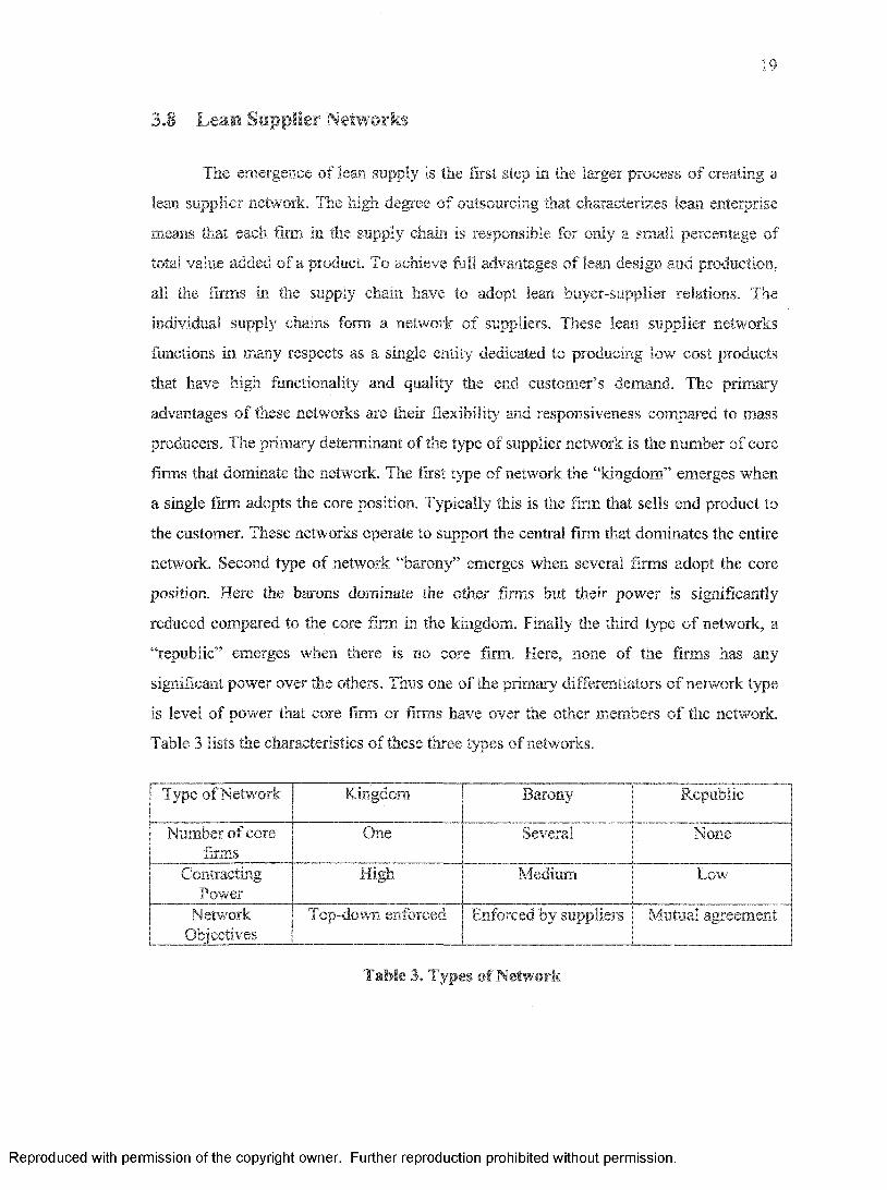
3.8 Lean Supplier Networks
The emergence of lean supply is the first step in the larger process of creating a
lean supplier network. The high degree of outsourcing that characterizes lean enterprise
means that each firm in the supply chain is responsible for only a small percentage of
total value added of a product. To achieve full advantages of lean design arid production,
all the firms in the supply chain have to adopt lean buyer-supplier relations. The
individual supply chains form a network of suppliers. These lean supplier networks
functions in many respects as a single entity dedicated to producing low cost products
that have high functionality and quality the end customer’s demand. The primary
advantages of these networks are their flexibility and responsiveness compared to mass
producers. The primary determinant of the type of supplier network is the number of core
firms that dominate the network. The first type of network the “kingdom” emerges when
a single firm adopts the core position. Typically this is the firm that sells end product to
the customer. These networks operate to support the central firm that dominates the entire
network. Second type of network “barony” emerges when several firms adopt the core
position. Here the barons dominate the other firms but their power is significantly
reduced compared to the core firm in the kingdom. Finally the third type of network, a
“republic” emerges when there is no core firm. Here, none of the firms has any
significant power over the others. Thus one of the primary differentiators of network type
is level of power that core firm or firms have over the other members o f the network.
Table 3 lists the characteristics of these three types of networks.
Type of Network Kingdom Barony Republic
Number of core firms
One Several None
ContractingPower
High Medium Low
NetworkObjectives
Top-down enforced Enforced by suppliers Mutual agreement
Table 3, Types of Network
Reproduced with permission of the copyright owner. Further reproduction prohibited without permission.

20
3.9 Performance Metrics in Supply Chain Management
A key element of improved supplier relationships is the presence of an objective
performance measurement system, which is used to ensure that both parties are operating
according to expectations and are meeting stated objectives. [14] Developing and using
performance measures are an essential function of management. Managers give
directions and achieve control through the use of performance measures. The key
question in supply chain management is how to coordinate the efforts of every firm in
supply chain and every employee of those firms.
Performance measures drive behavior in any system. The selection of
performance measures is crucial inside a firm and throughout the supply chain. Managers
coordinate behavior of their employees and of their partners in the supply chain by use of
performance measures.
The ideal performance measure pushes every firm in the supply chain and all
employees in each firm to direct all of their efforts to increasing the profits made by
everyone in the supply chain. The problem is that there is no perfect performance
measure which will always push firms and their employees in both the short term and
long term to make best decision for the long term benefit of supply chain. Key
performance measures that can be used in supply chain are: revenue, logistic costs,
logistic profit contribution, return on inventory, return on assets etc. [16]. The companies
should try to develop customer driven supply chain measures.
3.10 Supply Chain Management and Information Technology
Supply chain management is driven by the customer. It requires communication
to all participants in the supply chain of the customer’s needs and wants as well as how
well these needs and wants are being met. To facilitate managing the linkages in the
supply chain many types of software tools have been developed. These software
programs are not the strategy, rather they are the tools to implement a firm’s strategy.
The strategy is to focus the entire supply chain on satisfying the needs of the customer.
Reproduced with permission of the copyright owner. Further reproduction prohibited without permission.
21
Installing and using these tools is not the goal of the firm: the goal is to improve its
supply chain management. Many organizations place huge bets on technology and other
supply chain projects with little understanding of payoffs and the risks. The software
supply is abundant and vendors constantly produce new products. The manager is on his
own in evaluating a solution in the form of software or technique in terms of its fit with
company needs. [15]
There are a variety of software packages for each link in supply chain. The
available software can be divided roughly into three major categories. The first one
focuses on the internal linkages (i.e. software integrating own firm), the second software
links the firm to the customers and the third links firm to suppliers. The structure and use
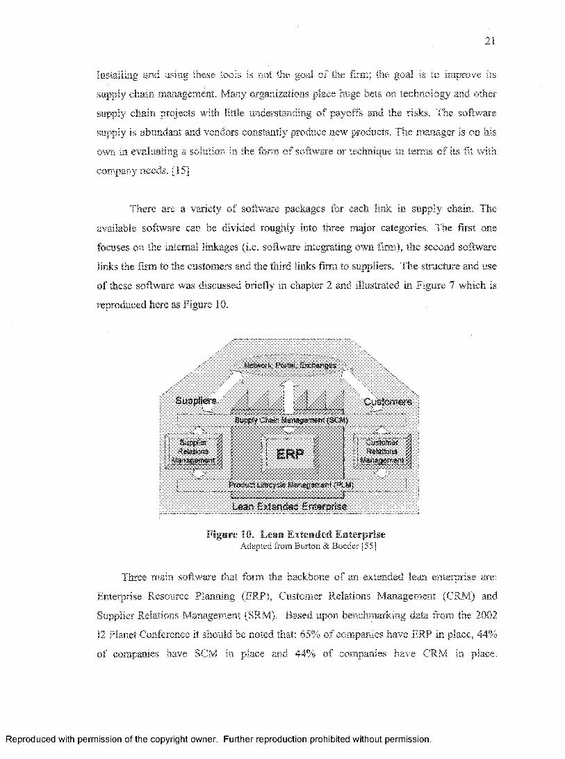
of these software was discussed briefly in chapter 2 and illustrated in Figure 7 which is
reproduced here as Figure 10.
Suppliers
i j Relations !
Network, Pcrtai, Exchanges
r.Customers
; \ill
ERPir' Custcsme: ”| I ■I: Relations j i
i Marwgfflnrantj
Product Ufscycte Management fPLM)
Lean Extended Enterprise
Figure 111. Lean Extended Enterprise Adapted from Burton & Boeder [55]
Three main software that form the backbone of an extended lean enterprise are:
Enterprise Resource Planning (ERP), Customer Relations Management (CRM) and
Supplier Relations Management (SRM). Based upon benchmarking data from the 2002
12 Planet Conference it should be noted that: 65% of companies have ERP in place, 44%
of companies have SCM in place and 44% of companies have CRM in place.
Reproduced with permission of the copyright owner. Further reproduction prohibited without permission.
22
In the following sections, we will discuss issues related to inventory management
within an organization and across several organizations within a supply chain.
Inventories in supply chain can be divided into four categories:
1. Raw materials - These are the components, subassemblies, or materials that are
purchased from outside the plant and used in fabrication/ assembly processes
inside the plant.
2. Work in progress - WIP includes all unfinished parts or products that have been
released to a production line.
3. Finished goods inventory: It includes finished product that has not been sold.
4. Spare parts - These are components that are used to maintain or repair production
equipment.
3.11 Reasons for Holding Inventory
a. Raw Materials: If a company could receive raw materials from its suppliers in just-in-
time fashion, it will not need to carry any raw materials inventory. Since this is very
difficult to happen, all manufacturing systems carry stocks of raw materials. Three main
factors influence the size of these stocks.
1. Batching: Quantity discounts from suppliers, limited capacity o f the plant’s
purchasing function, and economies of scale provide incentives to order raw
materials in bulk. Inventory that addresses the batching considerations is
referred as cycle stock.
2. Variability: Due to variability in various manufacturing processes the extra
stocks are planned for directly as a safety stock.
3. Obsolescence: The changes in demand or design can render some materials
obsolete. This inventory is termed as obsolete inventory.
b. W ork in Progress: Despite JIT goal of zero inventories, firm can never operate a
manufacturing system with zero WIP since zero WIP implies zero throughput. Under
Reproduced with permission of the copyright owner. Further reproduction prohibited without permission.

23
realistic conditions actual WIP levels frequently exceed the critical WIP level by large
amount, WIP can be divided into five categories as:
1. Queuing: if parts are waiting for resources
2. Processing: if part is being worked on by a resource
3. Waiting for batch: if WIP has to wait for other jobs to arrive in order to form a
batch.
4. Moving: if it is actually being transported between resources.
5. Waiting to match: if it consists of components waiting at an assembly operation
for their counterparts to arrive so that an assembly can occur.
As illustrated in Figure 11 below, the fraction of WIP in most manufacturing
systems that is actually moving or being processed is small. The majority of WIP is in
queue, waiting for batch, or waiting for match. Clearly, a WIP reduction program must
address these later categories.
W a:t:- r
ig for batch
Moving
Queuing
Figure II. Breakdown of WIP in Manufacturing Systems
c. Finished Goods Inventory: If a company is able to ship everything it produces
directly to customers as soon as processing is complete, there will be no need for FGI.
Although some manufacturing systems can achieve this, many cannot. The basic reasons
Reproduced with permission of the copyright owner. Further reproduction prohibited without permission.
24
for carrying FGI are: Customer responsiveness, batch production, forecast errors,
production variability, and seasonality. Ail these factors interact with each other.
d. Spare Parts: Spare parts are not used as direct inputs to finished products, but they do
support the production process by keeping the machine running. In many systems the
dollar value of inventory involved is not large but the consequences o f shortfalls can be
severe. In theory spare parts inventory systems are not much different from FGI systems.
In both parts axe stocked, possibly in batches to satisfy an uncertain demand process with
some level of service.
3.12 Managing the Inventory
The objective in managing the inventory is to have them available when needed
by the production process without carrying any more inventory than necessary. Some
strategies can enhance our ability to do this for all parts while others are economically
viable for only certain classes of parts. A few strategies are discussed below.
a. Improved Forecasting and Scheduling:
Due to long manufacturing cycle times and purchasing lead times, companies are
required to purchase at least some of the materials before they have firm customer orders.
In short term company may not have any option other than to maintain safety stock of
raw materials but in long term, company can improve the situation by following policies
such as: improving forecasting, reducing the cycle times, and improving scheduling.
b. ABC Classification:
In most manufacturing systems, a small fraction of the purchased parts represent a
large fraction of the purchasing expenditure. To have maximum impact management
should focus on these parts. To achieve this, ABC classification for purchased parts and
materials is used. ‘A’ parts are the first 5 to 10 percent of parts accounting for 75 to 80
percent of total annual expenditures. ‘B5 parts are the next 10 to 15 percent of parts
accounting for 10 to 15 percent of annual expenditure. ‘C ’ parts are the bottom 80 percent
Reproduced with permission of the copyright owner. Further reproduction prohibited without permission.
25
or so of the parts accounting for only 10 percent or so of total annual expenditure.
Because their number is relatively small and their cost is high it makes sense to use
sophisticated, time consuming methods to tightly coordinate the arrival of A parts. But
such efforts are not warranted for C parts. The B parts are in-between so they deserve
more attention than € parts but not as much as the A parts.
d. Just-In-Time:
The way to maintain the absolute minimum level of inventory of a part is to
coordinate deliveries with use in the production process. This is the idea behind JIT. A
typical JIT contract with supplier calls for frequent deliveries in small quantities closely
matched to what is required by the production schedule. To give suppliers reasonable
chance of meeting delivery requirements well managed JIT procurement systems provide
visibility of production schedule to suppliers. In concept JIT systems are very attractive.
However in order for them to work suppliers must be reliable, with regard to both
delivery timing and quality.
e. Setting Safety Stock/ Lead Times for Purchased Components:
It makes sense to link the purchases of expensive parts close to the production
schedule. In MRP language this means that parts should be ordered on lot-for-lot basis.
This approach is different from JIT because the parts are ordered according to planned
schedule, rather than having them delivered in synchronization with actual production.
The main drawback of this approach is that if schedule changes, production of the desired
amounts may be impossible due to lack of appropriate raw material. This implies that
short delivery lead times are less difficult to work with than long ones.
f. Setting O rder Frequencies for Purchased Components:
JIT and lot-for-iot purchasing schemes are reasonable options for part A and they
might work for intermediate B parts but are generally not appropriate for inexpensive C
parts. It doesn’t make sense to order screws, washers, etc to be delivered in tight
synchronization with production schedule. The increased risk of stockouts and extra
purchasing can’t be justified by reductions in inventory investment. The problem of
Reproduced with permission of the copyright owner. Further reproduction prohibited without permission.
26
managing inexpensive purchased parts can be thought of in terms of lot sizing. The
essential economic tradeoff is between inventory investment and purchasing cost. Lot
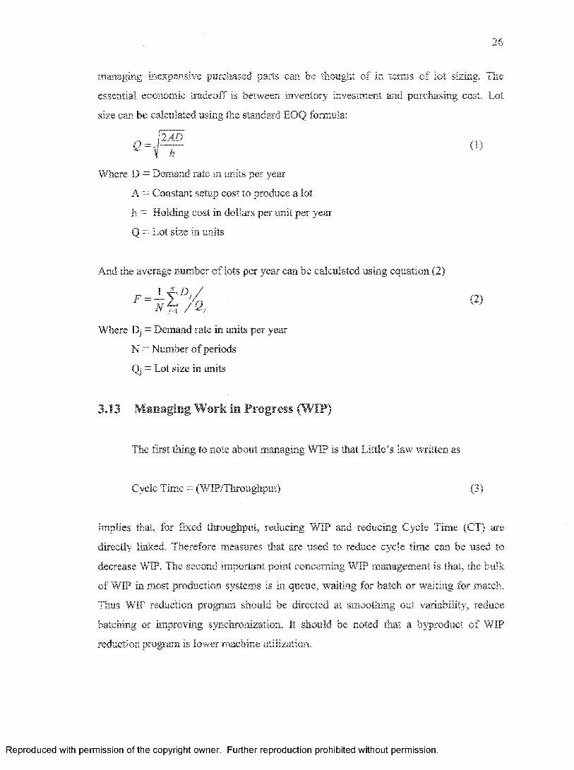
size can be calculated using the standard EOQ formula:
Where D = Demand rate in units per year
A = Constant setup cost to produce a lot
fa = Holding cost in dollars per unit per year
Q = Lot size in units
And the average number of lots per year can be calculated using equation (2)
Where Dj = Demand rate in units per year
N = Number of periods
Qj = Lot size in units
3.13 Managing Work in Progress (WIP)
The first thing to note about managing WIP is that Little’s law written as
implies that, for fixed throughput, reducing WIP and reducing Cycle Time (CT) are
directly linked. Therefore measures that are used to reduce cycle time can be used to
decrease WIP. The second important point concerning WIP management is that, the bulk
of WIP in most production systems is in queue, waiting for batch or waiting for match.
Thus WIP reduction program should be directed at smoothing out variability, reduce
batching or improving synchronization. It should be noted that a byproduct of WIP
reduction program is lower machine utilization.
(2)
Cycle Time = (WIP/Throughput) (3)
Reproduced with permission of the copyright owner. Further reproduction prohibited without permission.
27
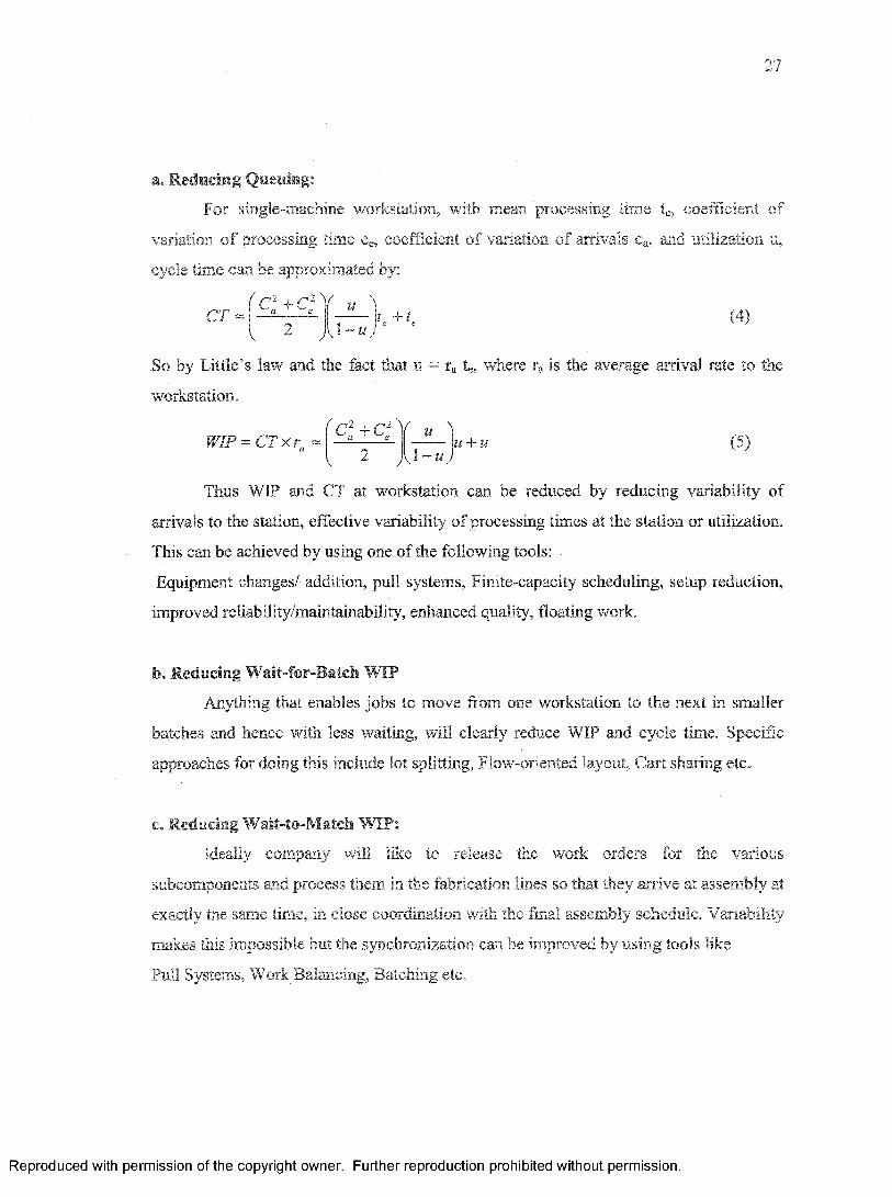
a. Reducing Queuing:
For single-machine workstation, with mean processing time te, coefficient of
variation o f processing time ce, coefficient of variation of arrivals ca, and utilization u,
cycle time can be approximated by:
CTcl + cl Y u '
l — ut „ + (4)
So by Little’s law and the fact that u = ra te, where ra is the average arrival rate to the
workstation.
WIP = CT x r ( C l + C ] \ f u \[ 2 J1.1 - u )
u + u (5)
Thus WIP and CT at workstation can be reduced by reducing variability of
arrivals to the station, effective variability of processing times at the station or utilization.
This can be achieved by using one of the following tools:
Equipment changes/ addition, pull systems, Finite-capacity scheduling, setup reduction,
improved reliability/maintainability, enhanced quality, floating work.
b. Reducing Wait-for-Batch WIP
Anything that enables jobs to move from one workstation to the next in smaller
batches and hence with less waiting, will clearly reduce WIP and cycle time. Specific
approaches for doing this include lot splitting, Flow-oriented layout, Cart sharing etc.
c. Reducing Wait-to-Match WIP:
Ideally company will like to release the work orders for the various
subcomponents and process them in the fabrication lines so that they arrive at assembly at
exactly the same time, in close coordination with the final assembly schedule. Variability
makes this impossible but the synchronization can be improved by using tools like
Pull Systems, Work Balancing, Batching etc.
Reproduced with permission of the copyright owner. Further reproduction prohibited without permission.
28
3.14 Managing Finished Goods Inventory (FGI)
Finished goods inventory acts as buffer between production and demand. Such a
buffer may be needed to insulate customers from manufacturing cycle time, perhaps to
provide “instant” delivery, to absorb variability in either the production or demand
process or to level out capacity loading (due to seasonality). These imply that anything
that links production and demand processes more closely will allow less FGI to be
carried. Options for doing this include improved forecasting, dynamic lead time quoting,
cycle time reduction, and cycle time variability reduction, late customization, balancing
labor, capacity and inventory.
3.15 Managing Spare Parts
Managing spare parts is an important component of overall maintenance policy,
which can be a major determinant of operational efficiency in manufacturing system.
Because of it’s importance and complexity, a wide variety of spare parts practices are
observed in industry.
There are two distinct types of spare parts, those used in scheduled preventive
maintenance and those used in unscheduled emergency repairs. Scheduled maintenance
represents a very predictable demand source. The standard MRP logic is probably
applicable to these parts. On the other hand unscheduled emergency repairs are by
definition unpredictable. There using MRP logic for these parts tends to work poorly.
Various approaches such as Backorder Model, Stockout Model can be used for
m aintain ing sufficient safety stock of spare parts whose demand is unpredictable.
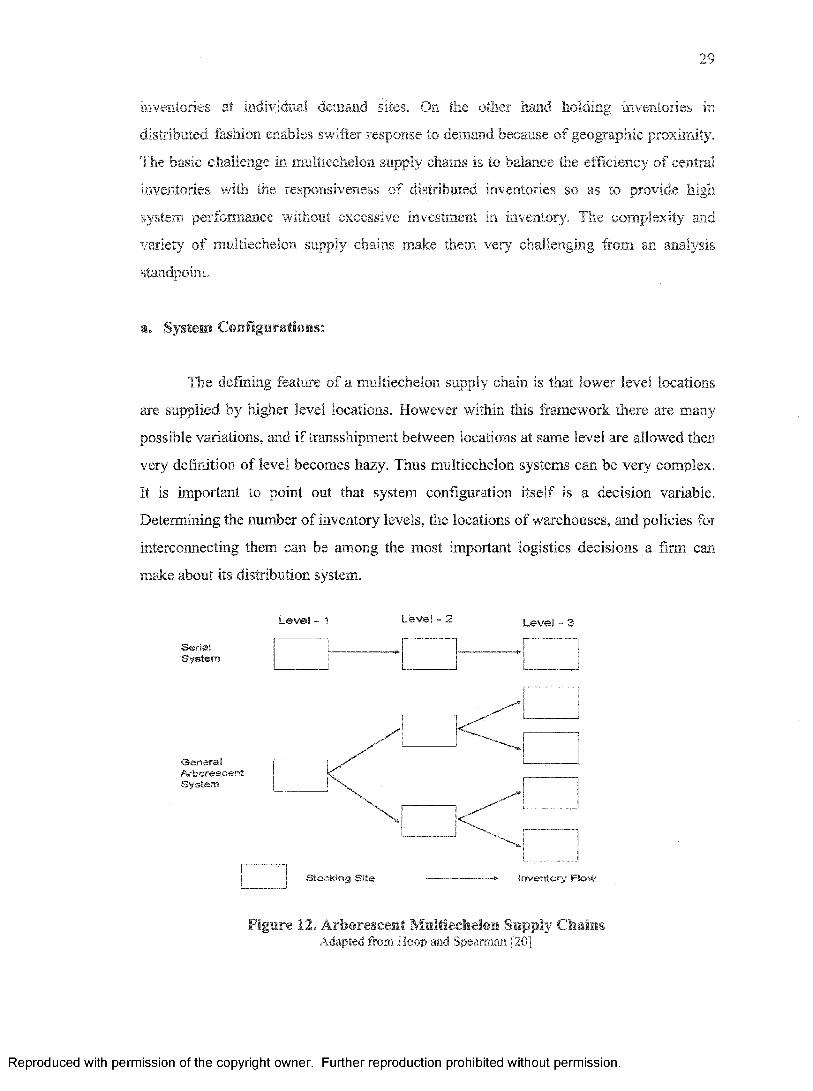
3.16 Multiechelon Supply Chains
Many supply chains including those for spare part, involve multiple levels as well
as multiple parts. Inventories can be stocked in central location such as warehouse or
distribution center which allows holding less safety stock than holding separate
Reproduced with permission of the copyright owner. Further reproduction prohibited without permission.
29
inventories at individual demand sites, On the other hand holding inventories in
distributed fashion enables swifter response to demand because of geographic proximity.
The basic challenge in multiechelon supply chains is to balance the efficiency of central
inventories with the responsiveness of distributed inventories so as to provide high
system performance without excessive investment in inventory. The complexity and
variety of multiechelon supply chains make them very challenging from an analysis
standpoint.
a. System Configurations:
The defining feature of a multiechelon supply chain is that lower level locations
are supplied by higher level locations. However within this framework there are many
possible variations, and if transshipment between locations at same level are allowed then
very definition of level becomes hazy. Thus multiechelon systems can be very complex.
It is important to point out that system configuration itself is a decision variable.
Determining the number of inventory levels, the locations of warehouses, and policies for
interconnecting them can be among the most important logistics decisions a firm can
make about its distribution system.
L e v e l - 1 Level - 2
SerialSy stem
G eneralA rborescentS y stem
Level - 3
Stocking Site i n v e n t o r y F lo w
Figure 12. Arborescent Multiechelon Supply ChainsAdapted from Hoop and Spearm an [20]
Reproduced with permission of the copyright owner. Further reproduction prohibited without permission.
30
This study focuses on a three level serial, single product supply chain system as
shown on top of Figure 12.
b. Performance Measures:
To make design decisions or develop a model, it is essential that desired system
performance be specified in concrete temis. Few performance measures are discussed
here.
L Fill Mate - It is the fraction of demands that are met out of stock. This could apply at
any level in the system. However measure applied to higher levels is only a means to an
end. It is the performance of the low levels that actually service customers that
determines the ultimate performance of the system.
ii. Backorder Level - This is the average number of orders waiting to be filled. This
measure applies to the systems where backordering occurs.
IM. Lost Sales - It is the number of potential orders lost due to stockout. This measure
applies to systems in which customers go elsewhere rather than wait for backordered
item.
iv. Probability of Delay - This is the likelihood that an activity will be delayed for lack
of inventory. This measure is often used in systems where high reliability is required.
c. The BiillwMp Effect:
An important issue that arises in multiechelon supply chains is that of channel
alignment. This refers to coordination of policies between various levels and can involve
information sharing, inventory control and transportation, among other management
decisions. The natural response to the complexity of multiechelon supply chains is to
treat the various levels independently. That is allowing each level to use local information
to implement locally “optimal” policies. Consequence of this is the bullwhip effect,
which refers to the amplification of demand fluctuations from the bottom of supply chain
Reproduced with permission of the copyright owner. Further reproduction prohibited without permission.

31
to the top. Figure 13 illustrates the bullwhip effect. The demand at the retail level seems
to be steady but at the manufacturer’s level it is volatile. The amplification of variability
as we go up the supply chain is a result of bullwhip effect.
1400i
1200-
1000 -
800-
600-
Q
200 '
Jan Feb Mar Apr May Jun Jui Aug S ep Oct Nov Dec
Time
El Retail Orders to Distributors ■ Distributor Orders to Manufacturers
Figure 13. Variation in Demand at Different Levels of Supply Chain A dapted from Hoop and Spearman [20]
3.17 Flow in Supply Chain
One of the key attributes of a successful winner in today’s highly competitive
marketplace is the ability to respond rapidly to the end consumer demand. To maximize
competitive advantage all members within the supply chain should "seamlessly” work
together to serve the end consumer. The main idea surrounding partnership sourcing is
that via closer ties and the resulting information sharing the partners will be more able to
effectively meet their customers' demands. Basically the pipeline is a mechanism by
which materials and information flow through a supply chain. Pipelines are smooth, well
defined passages enabling undisrupted movement, therefore requiring some form of
Reproduced with permission of the copyright owner. Further reproduction prohibited without permission.

32
design by the supply chain members. All companies belong to a supply chain but
unfortunately not all have developed to operate effective pipelines. The term "pipeline
management" was first coined by Forrester. As outlined by Farmer and Van Amstel the
concept is relevant to many situations where the organizational system is required to
balance a flow of incoming materials against outgoing components/products.
To compete effectively in the marketplace much pressure has been exerted on
supply chains and individual companies to improve pipeline performance by optimizing
their response to customer demand. As an important contribution to this improvement,
organizations have implemented specific pipeline process improvement techniques such
as just-in-time (JIT) and manufacturing resources planning (MRP). Methodologies such
as "lean manufacturing" have shown improvements to a whole host o f industries, most
notably the automotive sector where extensive research has been carried out. More
recently this approach has been broadened to encompass "lean thinking" and shown to
apply to a very wide range of industries. [17]
a. Functional Flows in Supply Chain
Flows within a supply chain can be divided into four categories based upon
function they serve. Value creation is achieved by simultaneous integration of these four
critical supply chain flows:
I. Product and Service Flow - which represents the value-added movement of
products and services from the raw-material provider to end-customers. Product
value is increased through physical modification, packaging, market proximity,
customization, service support, and other activities that enhance product
desirability from the end-customer's viewpoint.
i i Market Accommodation Flow - which reflects post-sales service
administration and reverse logistics, including product recalls and recycling.
Market accommodation also enables effective supply chain planning through
exchanging information on sales and product use. Examples include product
customization requirements, point-of-sale (POS) data, end-customer consumption,
Reproduced with permission of the copyright owner. Further reproduction prohibited without permission.
33
and warehouse releases, The market-focused flow provides supply chain
participants with channel visibility regarding timing and location of product
consumption. Improved overall planning and operations result when participants
share a common understanding of demand and consumption patterns.
Hi Information Flow - which is the bi-directional exchange of transactional data
and inventory status information among supply chain partners. Typical examples
are forecasts, purchase orders, order acknowledgments, shipping and inventory
information, invoices, payments, and replenishment requirements. Information
exchange initiates, controls, and records the product-service value flow and
market accommodation flow.
iv. Cash Flow - which generally moves in the reverse direction of the value-
added activities. In situations involving promotions and rebates, however, cash
may flow in the same direction as products and services. Cash-flow velocity and
asset utilization are essential to superior logistics performance.
These four flows occur in all distribution channels. Yet if not coordinated
and integrated among the channel participants, they can be characterized by delay,
redundancy, and inefficiency. To improve flow across a supply chain, individual
competencies related to operations, planning and control and behavioral
management must be integrated [9].
b. Physical Flows in Supply Chain
If we focus on the physical nature of entities flowing within the supply
chain, only two types of flows exist: Information flow and material flow. Lean thinking
emphasizes streamlining these two types of flows to enhance the value creation process.
Traditionally, productivity strategies have focused mainly on the material flow. It must be
emphasized that information flow is equally critical if we are to improve the efficiency of
the supply chain.
Reproduced with permission of the copyright owner. Further reproduction prohibited without permission.
34
I. Information Flow
The major technology behind improved information flow was the advent
of electronic data interchange (EDI), It offers greatly improved information flows
and is an extremely important aspect within leading organizations in the fight to
decrease lead-times. However, while the introduction of EDI in many companies
has offered marked improvement in the speed of transmission of orders (once
sanctioned), the current information flow in the vast majority of supply chains is
still far from ideal. Unfortunately, in all too many instances the old problems of
distortion and magnification of order information remain, not least because the
many decision processes which still remain block rapid data transference to where
it is really needed.
The main constraint to enriching a supply chain with market sales data is
the common attitude that information is power. As a consequence of the
traditional culture companies will deliberately distort order information to mask
their intent not only to competitors but even to their own suppliers and customers,
unbelievable though this may seem. In contrast managers can and should redesign
their business processes to gain competitive advantage and must include improved
information flow within their new strategy.
Market sales data is the information catalyst for the whole supply chain,
holding undiluted data describing the consumer demand pattern. Therefore, the
best way to ensure everyone in the supply chain gets the most up to date and
useful information is to feed each level of the supply chain directly with the
market sales data. Managers should, therefore, be challenging and questioning
mechanisms within pipeline, structures which delay order information through the
supply chain.
In the traditional supply chain the retailer is the only player who has direct
sight of consumer demand; all other members only have the orders from their
immediate customer, (i.e. the warehouse only has sight of the distributor's orders).
Reproduced with permission of the copyright owner. Further reproduction prohibited without permission.
35
Therefore, in the traditional mode the market information is distorted initially by
the retailer and further distorted with each successive link in the chain. However,
in the information streamlined supply chain each player, no matter how far
upstream, receives the marketplace data directly.
II. M aterial Flow
The concept of simplified material flow is not a new one, in fact the
principles can be traced at least as far back as the 16th Century, during which time
the Venice arsenalotti regularly delivered a war galley on a daily basis. In more
recent times the principles have been adopted by Womack and Jones and can be
seen to underpin the Lean Thinking paradigm and the associated concept of Value
Stream Management. If material flow is not simplified numerous symptoms are
clearly visible that result in ineffective product delivery process performance.
Simplified material flow can be achieved via the application of the 12 simplicity
rules. These rules are based upon the fundamental theoretical and practical work
started in this field by Jay Forrester and Jack Burbidge and has been further
extensively developed by Towill. [18]
Rule 1: Only make products that can be quickly dispatched and invoiced to
customers, highlights the need for companies to be pull/customer driven.
Rule 2: Only make in one time bucket those components needed for assembly in
the next, emphasizes the need to minimize work-in-progress stock levels.
Rule 3: Streamline material flow and minimize throughput time, is of critical
importance to all products. Compression of material, information and financial
lead times dramatically improves the integration and performance of supply
chains. Information lead times can be reduced via the use of the shortest planning
periods,
Reproduced with permission of the copyright owner. Further reproduction prohibited without permission.

36
Rule 4. Furthermore, adherence to this rale will reduce the use of old and less
accurate information thereby improving forecast accuracy and reducing buffer
stocks.
Rale 5: Only take deliveries from suppliers in small batches as and when needed
for processing and assembly is a well recognized approach to reducing in-bound
inventory levels.
Rule 6: Synchronization of time buckets through the chain. Lack of
synchronization results in buffer stocks at every location where the time buckets
differ. Consequently information lead times are elongated and out-of date data is
frequently used as a result of conflicting time buckets in the planning process.
Rule 7 relates to the need to avoid the conflicting objectives o f serving different
markets by a single supply chain strategy. Hence, by forming natural clusters of
products and designing processes appropriate to each value stream the
requirements of diverse customer requirements can be best served.
Rule 8: elimination of all uncertainties in all processes, Rule 8 is universal and
only by aiming for this goal will simplified material flow be truly achieved. If the
uncertainties in the process are not eliminated the result is poor and variable
quality levels and excessive lead times adversely impact on customer sendee and
raw material inventory levels.
Rule 9 relates to the need for a structured approach to change.
Rule 10: Highly visible and streamlined information flows. Rule 10 is important
to the simplification of material flow for all supply chains. It Is this information
that co-ordinates, controls and synchronizes the flow of material.
Rule 11 relates to the need to use proven and robust decision support systems in
the management of the supply chain so scientific rigor as opposed to gut intuition
guides strategy.
Reproduced with permission of the copyright owner. Further reproduction prohibited without permission.
37
The final Male 12 Is of critical importance to all types of products and related
supply chains. The operational target of the seamless supply chain needs to be
commonly accepted and shared by all members so to facilitate the arduous task of
change.
3.18 Summary
In summary this chapter provides a general background on the subject of supply
chain and its management. While there is ample information on issues in supply chain
management, there is a lack of cohesive approach utilizing systems perspective for
solving day to day problems that supply chain managers face in today’s global
manufacturing environment. We hope, this study will result in a set of practical
guidelines that the managers can implement to streamline their supply chains. To get
closer to the heart of the topic of this dissertation, we need to explore the published
literature specifically in the area of supply chain dynamics and bullwhip effect. In next
chapter, we look at the published literature
Reproduced with permission of the copyright owner. Further reproduction prohibited without permission.

38
Chapter - 4
LITERATURE SURVEY
Supply chain management (SCM) is the practice of coordinating the design,
procurement, and flow of goods, services, information and finances, from raw material
flows to parts supplier to manufacturer to distributor to retailer to consumer. This process
includes product design, order generation, order taking, information feedback and the
efficient timely delivery of goods and services, and typically involves many or more of
the business functions in firms that are linked to specific supply chains. Efficient and
effective supply chain management assists an organization in getting the right goods and
services to the place needed at the right time, in the proper quantity and at acceptable
cost. Managing this process involves developing and overseeing relationships with
suppliers and customers, controlling inventory, and forecasting demand, all requiring
constant feedback from every link in the chain.
To co-ordinate such a complex network is difficult and requires better
communication at each stage of the supply chain. The performance of a supply chain
depends upon a number of factors. Issues facing the supply chain in today’s shipbuilding
industry were mentioned in Table 2 in chapter 3. In this section, we look at the published
literature dealing with some of these issues.
4.1 The Impact o f ERP on Supply Chain Management
Ackkermans et al presented results from a Delphi study on the future impact of
enterprise resource planning (ERP) systems on supply chain management (SCM) [22].
The Delphi study was conducted with 23 Dutch supply chain executives of European
multi-nationals. Findings from this exploratory study were threefold. The following key
SCM issues were identified for coming years:
(1) Further integration of activities between suppliers and customers across
the entire supply chain.
(2) On-going changes in supply chain needs and required flexibility from IT.
Reproduced with permission of the copyright owner. Further reproduction prohibited without permission.
39
(3) More mass customization of products and services leading to increasing
assortments while decreasing cycle times and inventories.
(4) The locus of the driver’s seat of the entire supply chain.
(5) Supply chains consisting of several independent enterprises.
It was also concluded that there is only a modest role for EBP in improving future
supply chain effectiveness and a clear risk of ERP actually limiting progress in SCM.
ERP was seen as offering a positive contribution to only four of the top 12 future supply
chain issues:
(1) More customization of products and services.
(2) More standardized processes and information.
(3) The need for worldwide IT systems.
(4) Greater transparency of the marketplace.
The following key limitations of current ERP systems in providing effective SCM
support emerged as the third finding from this exploratory study:
(1) Their insufficient extended enterprise functionality in crossing organizational
boundaries.
(2) Their inflexibility to ever-changing supply chain needs.
(3) Their lack of functionality beyond managing transactions.
(4) Their closed and non-modular system architecture.
These limitations stem from the fact that the first generation of ERP products has
been designed to integrate the various operations of an individual firm. In modem SCM,
however, the unit of analysis has become a network of organizations, rendering these
ERP products inadequate in the new economy.
4.2 Made to Store (MTS) vs. Made to Order (MTO)
Hax and Candea proposed that there are two ways to determine whether a product
should be produced according to made to store (MTS) or made to order (MTO). The first
Reproduced with permission of the copyright owner. Further reproduction prohibited without permission.
40
criterion, was service consideration based on lead, times, and the second criterion was
economic considerations based on cost [38], In a working paper of MIT, the MTS and
MTO manufacturing strategies were compared, and the effect of inventory on delivery
time was evaluated [35], Donald et al first considered them as a set of strategies and
called them Production Positioning Strategy (PPS) [39], Howard ef al called it built to
store (BTS) and built to order (BTO) strategies, and named them Demand Response
Strategies, and considered them as the methods of response to customer demand [40],
Nguyen developed heavy traffic limit approximations for various performance measures
in hybrid MTO/MTS systems, governed by base-stock policies [41]. Wang and Yu
analyzed the integration of BTS and BTO strategy by a mathematical model and
computer programming [42]. In general, the main limitation of the past research is that
many researchers do not pay much attention on the integration of the typical strategies,
which is very important.
4.3 How Gillette Cleaned its Supply Chain
Duffey [23] discusses about the problems Gillette faced with its supply chain and
how it overcame them. Gillette failed to meet its goal for effective customer service.
Even though Gillette’s products were constantly in demand, they could not reliably ship
to its customer’s requirements. The major reason for this was its lackluster supply chain
performance. The table below gives an idea about the problems Gillette faced, and the
measures it took to counter them.
Reproduced with permission of the copyright owner. Further reproduction prohibited without permission.

41
Mo. Problems Faced Steps taken
1 Inventory levels decided based on planners experience, without taking forecast accuracy, demand volatility and manufacturing run frequency into account
Improved supply planning by taking into account new product launches, vendor flexibility, batch sizes, manufacturing flexibility, forecast accuracy and sourcinglocation.Collaborated with customers to make data uniform. In some cases JIT, where predictable demand.
2 No on-time shipments due to spikes in demand Segmented forecasting to accommodate spikes in demand resulting due to factors such as seasonality & promotions.
3 For promotions, dependence on dollar accuracy of forecast rather than unit accuracy - resulting in shipment inaccuracies.
Worked closely with sales to ensure dollar forecasts are translated into unit forecasts and that all parties are held accountable for final expectation.
4 No accountability, finger pointing Had members of both demand side and supply side on project team.Focus more on data.
5 Segmented supply chain process Integrated value chain organization
6 Different departments responsible for inventory planning, demand planning, promotions, customer service each one reporting to different Vice President.
Staff Co-located and under one management team & single point accountability (Cradle to grave approach}
7 Demand planning more focused on what company wanted to sell rather than how many could be sold
Demand not concentrated on financial targets, giving a true picture of demand.A dedicated manager for demand planning resulting in a less filtered view of demand.
8 Forecast Accuracy: 46 % ... Jan’03 Fill rates: 90 % ... Jan’03
Forecast Accuracy: 71 % ... Nov’03 Fill rates: 98 % ... Nov’03 Inventory reduction by 25 %Cost reduction by 3 %.
Table-4 Problems Faced by Gillette and Steps Taken
4.4 B ullw hip E ffect
Demand variability increases as one move up the supply chain away from the
retail customer and small changes in customer demand can result in large variation in.
orders upstream. This phenomenon is known as Bullwhip effect. This results in increased
cost and poorer service.
Reproduced with permission of the copyright owner. Further reproduction prohibited without permission.
42
The sources of variability can be demand variability, quality problems, strikes, etc.
Variability coupled with time delays in the transmission of information up the supply
chain and time delays in manufacturing and shipping goods down the supply chain create
the bullwhip effect.
The following can add to bullwhip effect
• No communication through the supply chain
Delay in flow of information and material
Large batch size
Neglecting to order in an attempt to reduce inventory
Inaccurate demand forecast
The bullwhip effect has been noted and assigned various causes across a range of
academic disciplines. Forrester stated that the principal cause of this was the difficulties
involving the information feedback loop among companies, and that such systems were
too complex for managerial intuition alone to address. Consequently, his remedy lay in
understanding the system as a whole, and modeling that system with system dynamics
simulation models [43]. Steraian proposed a simple beer distribution game which
simulated a supply chain with four players, retailer, wholesaler, distributor, and the beer
producer. In the game, customer orders were predetermined but were revealed only
period by period as the game progresses. The demand was constant in the first few
weeks, and then doubled and kept constant in the subsequent weeks. He found that
because of the demand change and the rational actions of the players, the information was
distorted, and the demand was amplified [44, 45]. Goodwin and Franklin also did some
work on this game [46]. Metters constructed a function to quantify and optimize the
discounted expected cost of the bullwhip effect in the supply chain. In the function the
inventory holding cost, production cost, and penalty cost of unsatisfied demand were
evaluated [47]. Lee et al analyzed the causes of the bullwhip effect, which were demand
forecast updating, order batching, price fluctuation, and rationing and shortage game.
They used an order-up-to-S, periodical model to quantify their effect and proposed some
approaches to reduce the bullwhip effect [36, 37], Towill discussed the industrial
Reproduced with permission of the copyright owner. Further reproduction prohibited without permission.
43
dynamics modeling in supply chains, and Towill and McCullen analyzed the impact of
agile manufacturing on supply chain dynamics [48,49], Song also built a simple model
developed from the beer game model and discussed the effect of seven causes on supply
chain dynamics (SCD), which were shortage game, capacity, information delay, poor
coordination, materials delay, demand signaling, and order batching [50], Fransoo
and Wouters proposed a mathematical model to measure the bullwhip effect in the supply
chain. In the model, the bullwhip effect at a particular echelon in the supply chain was
measured as the quotient of the coefficient of variation of demand generated by this
echelon and that received by this echelon. Then based on the model and the data from a
project, they discussed how to solve the problems in the measurement of supply chain
bullwhip effect [51]. Chen et al. analyzed the effects of demand forecasting, lead times,
and information in a simple supply chain, and concluded that the bullwhip effect could be
reduced by centralizing demand information [52]. In general, there is a lot of good
research in this domain, but the qualitative analysis of SCD and the discussion on its
effect on supply chain planning is not enough.
4.5 Managing Physical, Information and Financial Flows
According to Villa [24], managing different types of physical, information and
financial flows become a real challenge for managers and researchers, due to the
complexity of the problem. Supply chain management involves a variety of management
and technical issues, starting from distributed design of products and processes, the
decentralized but efficiently coordinated production of goods through suppliers
contracting and outsourcing to the coordination of third party logistics and multi
locations inventories. Often each supplier in the supply chain tries to maximize its own
profit, which conflicts with the overall performance goal of the supply chain as a whole.
The paper further states that an integrated supply chain can present significantly different
performance depending on the types of products and production flows involved.
Reproduced with permission of the copyright owner. Further reproduction prohibited without permission.
44
4.6 Supplier Relationship Management
Improving supply chain execution and leveraging the supply base has become
more critical than ever in achieving competitive advantage [25]. Technological
developments in the last 10 years aimed at improving the supply chain have mainly fallen
into two major areas: optimized Supply Chain Planning, and Customer Relationship
Management. However the successful Supply Chain Planning applications of the last
decade have been largely focused on optimizing resource utilization within a single
enterprise. This paper discusses about a new category of supply chain software
applications, called Supplier Relationship Management (SRM) which can dramatically
improve supply chain performance and empower a new level of supply base
management, and how it can fit into typical manufacturer’s supply chain process. SRM
solutions are aimed at helping manufacturers maximize the value of their supply base to
deliver strategic value. A comprehensive SRM solution supports a broad set of business
processes including:
1. Strategic Supply Management
2. Supply Chain Collaboration
3. Procurement Execution
4.7 Improving Extended Supply Chain Performance through Better
Control
Many manufacturers struggle with the challenges of shrinking product lifecycles,
increased complexity of outsourced or multi-tier supply chains, and volatile product
demand [26], Even after spending millions of dollars on ERP, APS, and Supply Chain
Event Management (SCEM) these systems rarely meet expectations. Moreover scope of
ERP and APS systems are limited to a single-enterprise. Communication, visibility and
control across the multi-tier system have become the most significant challenges for
today’s manufacturers.
The companies that can smoothly control the flow of materials while matching
supply and demand have a significant advantage, and more importantly they have better
Reproduced with permission of the copyright owner. Further reproduction prohibited without permission.
45
financial performance. Controlling supply chain means having the capability to either
increase or decrease material velocity across the entire supply chain.
4.8 Supplier Development and Supply Chain Management in Small
and Medium Size Enterprises
This paper [27] provides the outcomes of a supplier development and supply
chain management attitude survey designed to identify current trends in businesses within
supply chains. The analysis identifies the adaptation of supplier development and supply
chain management techniques. The relationships between customers and smaller
suppliers are also examined, giving an indication of the lack of effective adaptation from
the traditional adversarial relationships to the modem collaborative supply chain
relationships. The outcomes based on a survey of 400 small firms identify issues, which
businesses need to address to improve the performance of their supply chains, and so
improve their competitive position by grasping the benefits of effective supply chain
management
4.9 Information Systems Failure and Its Impact on the Supply Chain
Decision Process
The realization that many supply chain managers are still using strategies that
were devised for the pre-IS types of supply chains calls for a strategy that considers the
effect of In formation System Failure (ISF) in supply chain management decision making.
Rakotobe et al [28] proposed supply chain decision strategy that addresses the dynamic
multi-dimensional socio-technicai issues within a heedful supply chain. The framework is
based on the high reliability organization and supply chain management techniques.
Reproduced with permission of the copyright owner. Further reproduction prohibited without permission.

46
4.10 Implications ©ff Postponement for Supply Chain
With the increasingly sophisticated customer demand (e.g. product variety and
customization), supply chains have to be responsive to constantly changing markets. As
forecast and planning become very complex [29], producing and storing all types of
finished goods based on forecast will run a high risk of stock out and obsolescence while
lead times often makes make-to-order impossible. Therefore, postponement has been
increasingly used as an important supply chain strategy.
Postponement centers around delaying activities in the supply chain until real
information about the markets is available. The viability of postponement is determined
by the structure of the supply chain characteristics. On the other hand, postponement
affects the supply chain. The implementation of postponement often leads to the
reconfiguration of the supply chain. Postponement application has also resulted in a
blurring of warehousing, assembly and retail operations, and the warehouse is often the
place where final assembly, labeling and packaging are processed. By employing
postponement and combining it with a holistic view, some companies have managed to
improve the performance of the supply chain.
4.11 Very High Inventory, No Consistent Approach to Inventory
Management
This is also a common problem faced in the supply chain [30]. Various inventory
management methods are utilized by firms to minimize supply and demand imbalances in
the supply chain. The problem is generally complicated by the fact that the demand is
uncertain, which causes stock outs resulting in order not being filled.
In addition to the above issues discussed in the literature, other problems found
within a supply chain include high order fulfillment lead time [32], ineffective customer
Reproduced with permission of the copyright owner. Further reproduction prohibited without permission.
47
service [31], planning cycles not aligned [33] and a general lack of trust among supply
chain members [34],
High order fulfillment Lead Time results in the overall long lead times for the
company. Ineffective customer service results when the company is not able to meet its
customer demand on-time. If the planning cycles for the entire supply chain is not
aligned, it will result in bottlenecks throughout the system. A lack of trust between
customer and supplier equates to higher transaction costs since this will lead to
companies holding “safety” inventory at multiple stages in the supply chain.
For a company to be a world leader, it has to streamline its supply chain. Demand
forecast accuracy, perfect order, supply chain cost, and cash-to-cash cycle time are
the four most critical metrics a company can use to get a quick, balanced snapshot of its
supply chain performance. With these four metrics, a company can see how good a view
of demand it has, where it is making trade-offs between cost and service, and how well it
is managing the cash flow.
4.12 Summary
Published articles point to a number of issues related to the supply chain
management. Chief among these issues is the lack of integration of activities between
suppliers and customers across the entire supply chain. Other issues include bullwhip
effect, management of flow within the supply chain, supplier relations management,
impact of ERP and implications of postponement. A number of authors have focused on
one or two specific issues however there is lack of a cohesive approach to address all the
issues. For example, there is plenty of research in the area of supply chain dynamics, but
the qualitative analysis of SCD and the discussion on its effect on supply chain is not
enough. In general, the main limitation of the past research is that many researchers do
not pay much attention to the integration of multiple strategies. ERP’s were conceived to
improve integration of business activities however they suffer from insufficient extended
enterprise functionality and inflexibility to ever changing supply chain needs.
Reproduced with permission of the copyright owner. Further reproduction prohibited without permission.

48
4.13 Intent of Dissertation
This study strives to address the supply chain integration problem by looking at
the big picture via three methods; mathematical stochastic modeling, physical simulations
and computer based simulations. All three of these methods incorporate variability
associated with supply chains. Simulations in general are used extensively for modeling
complex systems because of their ability to incorporate system variability. We make the
distinction between physical simulation and computer based simulations. Physical
simulations are those where participants in a class room are assigned specific roles within
an organization and make decisions based upon the situation and rules given to them.
Performance metrics are used to track system performance. This is usually done in
multiple phases where productivity and management strategies are introduced and their
impact studied. Use of physical simulations in manufacturing and management training
has grown recently with the advent of Lean philosophy. Computer based simulations use
a computer software to model a system with all its inherent variability and track its
performance through a number of parameters. Computer based simulations can
incorporate much higher level of detail and resolution compared to physical simulations
however in terms of mimicking a real life system, physical simulations do a much better
job since they incorporate human interactions and dynamics.
To achieve the dissertation intent indicated above, the following chapters are
provided in succession. Existing mathematical models (both deterministic and stochastic)
are discussed in chapter-5. Application of base stock model and (Q, r) model are
discussed in chapter-6 and 7. Physical simulation models are discussed in chapter-8 and 9
and computer based simulation model is discussed in chapter-10.
Reproduced with permission of the copyright owner. Further reproduction prohibited without permission.

49
Chapter - 5
EXISTING MATHEMATICAL MODELS
Taylor’s principles of scientific management [59] were precursor to a host of
mathematical models designed to solve the problems associated with manufacturing
planning and control. These models formed the foundation for instruction in several
operations management (OM) areas like inventory control, scheduling, capacity planning,
forecasting and quality control. Of these areas, inventory control saw the development of
a variety o f mathematical models. These models can be subdivided into two broad areas.
Those that assumed a known demand, and those that assumed a stochastic demand. Hopp
and Spearman [20] provide a survey of existing mathematical models for analyzing
inventory management within a supply chain.
5.1 Deterministic Models
One of the earliest deterministic models came out of work of Ford W. Harris [58]
(1913). Harris’s Economic Order Quantity (EOQ) model has been widely studied. His
model makes the assumptions that:
1. Production is instantaneous
2. Delivery is immediate
3. Demand is deterministic
4. Demand is constant over time
5. Each production run incurs a constant setup cost
With these assumptions, he derived the following formula for calculating the total
inventory cost per product:
T ( 0 = — + — + c (6)2D Q
Where D = Demand rate in units per year
c = Unit production cost
Reproduced with permission of the copyright owner. Further reproduction prohibited without permission.
50
A = Constant setup cost to produce a lot
h = Holding cost in dollars per unit per year
Q = Lot size in units
The lot size that minimizes Y(Q) in the previous equation, is:
(7)
The Economic Production Lot Model (EPL) propose by Taft [60], modifies the EOQ
model to include finite and predictable production rate P.
^ h ( l - D / P )
Wagner-Whitin model [61] considers the problem of determining production lot size
when demand is deterministic but varies with time.
5.2 Stochastic Models
Statistical modeling of production and inventory control dates back to Wilson’s
work [62]. Wilson breaks inventory control problems into two parts:
1. Determining the order quantity, which is the amount of inventory that will
be purchased or produced with each replenishment.
2. Determining the reorder point, or the inventory level at which a replenishment,
will be triggered.
The following three models have attempted to address this issue with three
different approaches:
1. Newsboy Model - Considers only a single replenishment so the only issue is to
determine the order quantity in face of an uncertain demand.
2. Base Stock Model - Considers the replenishment of inventory one unit at a
time as random demand occurs. Thus, the only issue here is to determine the
AD h(l - D i P)Q(8)
Minimizing equation (8) yields:
I 1AD
Reproduced with permission of the copyright owner. Further reproduction prohibited without permission.
51
reorder point. The target inventory set for the system is known as the base
stock level.
3. (Q, r) Model - In this case the inventory is monitored continuously and demand
occurs randomly and possibly in batches. When the Inventory level reaches r,
an order of size Q is placed. After a lead time 1, during which a stockout may
occur, the order is received.
The Newsboy model, while being useful in certain situations, is not realistic in
case of a supply chain where multiple replenishments may be required. Thus we will look
at the last two models in detail and compare them in the context o f a two tier supply
chain. Base stock model is closer to the Lean concept of make one move one since the
replenishment quantity is one here. Realistically, it is not always possible to have order
quantities of one and economies of scale may dictate ordering in batches. (Q, r) model
addresses this need by providing a method for calculating both the order quantity and the
reorder point.
We first look at the Base Stock model and then (Q, r) model.
5.3 The Base Stock Model
The Base Stock model uses a continuous time frame and makes the following
assumptions:
1. Products can be analyzed individually. There are no product interactions.
2. Demands occur one at a time. There are no batch orders.
3. Any demand not filledfrom stock is backordered. There are no lost sales.
4. Replenishment lead times are fixed and known. There is no randomness in
delivery lead times.
5. Replenishments are ordered one at a time. There is no setup cost associated with
placing an order and no constraint on the number of orders that can be placed per
year.
Reproduced with permission of the copyright owner. Further reproduction prohibited without permission.
52
We make use of the following notations:
1 = Replenishment lead time (in days)
x — Demand during replenishment lead time (is units), a random variable
G (x) = P (X<=x) = ]£~-0P(0 > cumulative distribution function of demand
during replenishment lead-time; we will allow G to be continuous or discrete.
0 = E [X] mean demand (in units) during lead time 1
h = cost to carry one unit of inventory for one year (in dollars per unit per year)
b = cost to carry one unit of backorder for one year (in dollars per unit per year)
r = reorder point which represents the inventory level that triggers a replenishment
order;
R = r + 1 base stock level
S = r - 0, safety stock level
G (r) or S (R) = Fill rate i.e., Fraction of demand filled from stock is equal to the
probability that an order arrives before the demand for it has occurred.
We place an order when there are r units in stock and we expect a demand of 0 units
to occur while we are waiting for replenishment order to arrive. The inventory level is r -
0 when the order arrives. If s = r - 0 > 0, then we call this the safety s t o c k for the system.
Since finding r - 0 is equivalent to finding r (0 = constant), we can view this as the
problem of finding the optimal base stock (R = r + 1), or reorder point r, or safety stock
level (s = r - 0 ).
We can approach the problem of finding an optimal base stock level in one or two
ways. We can formulate a cost function and find a reorder point that minimizes this cost.
Or we can simply specify the desired customer service level and find the smallest r that
attains it. We will look at the second approach since customer satisfaction is one of the
key goals of Lean philosophy.
Reproduced with permission of the copyright owner. Further reproduction prohibited without permission.

53
We begin by analyzing the relationship between inventory, replenishment orders,
and backorders under a base stock policy. We distinguish between on-hand inventory,
which represents physical inventory in stock (cannot be negative), and inventory
position, which represents the balance of on-hand inventory, backorders, and
replenishment orders and is given by:
Inventory position = on-hand inventory' - backorders + orders (10)
Under the base stock policy we place a order every time a demand occurs. Hence,
the following relationship holds true at all times:
Inventory position = R (11)
Using equations (10) and (11), we can derive an expression for the performance
metric for meeting a specified service level.
Since lead times are constant, we know that all the other R - 1= r items either in
the inventory or on order will be available to fill new demand before the order in question
arrives. Therefore, the only way the order can arrive after the demand for it has occurred
is if demand during the replenishment lead time is greater than or equal to R ( that is,
X > R ). Hence, the probability that the order arrives before its demand (i.e., does not
result in backorder) is given by
Since all orders are alike, the fraction of the demand that are filled from stock is
equal to the probability that an order arrives before the demand for it has occurred, or
P (X < R) = P (X < R - 1) = G (R -1 ) = G(r) (12)
S(R) = G ( R - l ) = G(r) (13)
Reproduced with permission of the copyright owner. Further reproduction prohibited without permission.
54
Hence, G(r) or S(R) represents the fraction of the demand that will be filled from
stock. This is known as the fill rate and represents a measure of customer satisfaction and
hence its selection as a performance metric.
Base stock model is equivalent to the Japanese Kanban System, (with kanban size
of one) since, order quantity is one.
If li = annual cost to hold a unit of inventory and
b = annual cost of backorder
The condition for the optimal base stock level for this model is very similar to one for
Newsboy model and has been derived by Johnson and Montgomery [57],
G ( R * ) = - t - (14)h + b
Thus the optimal base stock level is the one for which the fill rate is given by
equation (14). This result makes intuitive sense, since increasing the holding cost h will
decrease R*, while increasing backorder cost b will increase R*. It should be noted that
when backorder and holding costs are equal the resulting fill rate is 0.5 and R* = 0, the
average demand during replenishment lead time, and therefore there are no safety stocks.
Cost Analysis:
We can formulate the quantitative cost analysis by first looking at the expression
for average inventory level. For most of the cases, unless there Is seasonal product
demand, the average inventory position can be expressed as:
Inventory Position = Average Inventory + Safety Stock
Average Inventory = Q/2
Safety Stock = s = r - 0
fO 1Therefore: Inventory Position = + r - 0 ) and
Investment in inventory = c x j ^ + r - f f j
Where c = unit cost of product in dollars
Reproduced with permission of the copyright owner. Further reproduction prohibited without permission.

55
Total Cost = Order Cost + ex[2 j
We will use these cost equations to compare the various cases later in chapter 6.
Primary Insights from the Model:
Base stock model has been widely researched in operations management
literature, partly because it is simple to analyze and can be applied to a wide rage of
situations. For instance, base stock can be used to control work releases in a multistage
production line or multiechelon supply chain. In summary, the primary insights from base
stock model are:
1. Reorder points control the probability of stockouts by establishing safety stock.
2. To achieve a given fill rate, the required base stock level (and hence safety stock)
will be an increasing function of both mean and standard deviation of the demand
during replenishment lead time.
3. Base stock levels in multistage production systems are very similar to kanban.
5.4 Application of Base Stock Model - An Example
We consider the example of an appliance store which sells various models of
refrigerators. We know from past experiences that the mean demand for a certain model
is 10 units per month, and replenishment lead time is one month. Therefore mean demand
during the replenishment lead time is 10 units. Thus known quantities are:
Average Demand = D = 10 units per month
Replenishment lead time, 1 = 1 months
Average demand during replenishment lead time, 0 = —x D = - x l O =10 units
Reproduced with permission of the copyright owner. Further reproduction prohibited without permission.

56
This example was adapted from the book by Hoop and Spearman [20] and
included here to illustrate the application of this model. Let us assume that the demand
for refrigerators follows Poisson distribution.
0 re~9 1 0 ’’e -10p(r) = Probability {Demand during lead time = r}= ———- = ---------
r! r\
' ' r 10*And G (r) Cumulative Probability Distribution = ^ p (k ) = ^ ----------k =o k =o
The Poisson distribution is a good modeling choice for supply chains where
demands occur one by one and do not exhibit cyclic fluctuations. It is completely
specified by only one parameter, the mean and is therefore convenient when one does not
have information concerning the variability of demand. The standard deviation of the
Poisson is equal to the square root of the mean.
'f IViCllbSCmi : . ■ fr T z m - - : - .0 0 0 12 0.095 0.7921 0 0 13 0.073 0.8642 0.002 0.003 14 0.052 0.9173 0.008 0.01 15 0.035 0.9514 0.019 0.029 16 0.022 0.9735 0.038 0.067 17 0.013 0.9866 0.063 0.13 18 0.007 0.9937 0.09 0.22 19 0.004 0.9978 0.113 0.333 20 0.002 0.9989 0.125 0.458 21 0.001 0.99910 0.125 0.583 22 0.000 0.99911 0.114 0.697 23 0.00 1.00
r= 14h n
r*= 12
Table 5. Fill Rates G(r) for Various Values of r
We need to calculate the base stock level and safety stock for a given fill rate.
Table 5 is constructed using the above formulae. From this table, we find the value of r
that will satisfy a given fill rate. For example, if we want a fill rate G(r) of 90%, the
closest number above 0.9 is 0.917 which corresponds to a value of r = 14.
Hence safety stock s = r ~ 0 = 14-10 = 4
Reproduced with permission of the copyright owner. Further reproduction prohibited without permission.
57
The optimal base stock level is the one for which the fill rate is given by equation
(9) which was derived by Johnson and Montgomery' [57] and give here again.
G(r*) = A 0 5 )h + b
Where h = annual cost to hold a unit of inventor}' and
b = annual cost of backorder
If we assume the annual holding cost h to be $15 and annual cost of a backorder b
to be $ 40, then the fill rate corresponding to optimal base stock level will be given by:
h 4 0G(r*) = = ----- — = 0.727
h + b 15 + 40
This fill rate corresponds to an optimal base stock level of r* =12 from table 4.
This example points out the utility of Base Stock Model. According to the model,
if the manager of the appliance store desires a fill rate of 90% then he should maintain a
base stock level o fR = r + l = 1 4 + l = 15 refrigerators. However, if the manager’s
primary concern is to minimize the cost associated with inventory then he should carry a
base stock level of R* = r* + 1 = 12 + 1 = 13. The corresponding fill rate will drop down
as in this case to 72.7% leading to a lower customer satisfaction.
5.5 The (Q, r) model
The first formal publication of the (Q, r) model was done by Wilson in 1934 [66],
From the modeling perspective, the (Q, r) model is identical to the base stock model
except that:
1. A fixed cost is associated with each replenishment order.
2. Orders may be batched.
3. A constraint on the number of replenishment orders per year exists.
Reproduced with permission of the copyright owner. Further reproduction prohibited without permission.
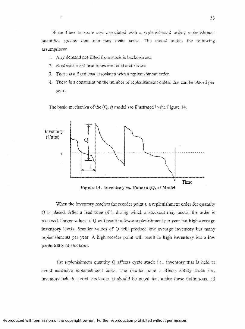
58
Since there is some cost associated with a replenishment order, replenishment
quantities greater than one may make sense. The model makes the following
assumptions:
1. Any demand not filled from stock is backordered.
2. Replenishment lead times are fixed and known.
3. There is a fixed cost associated with a replenishment order.
4. There is a constraint on the number of replenishment orders that can be placed per
year.
The basic mechanics of the (Q, r) model are illustrated in the Figure 14.
Inventory(Units)
r
TimeFigure 14. Inventory vs. Time in (Q, r) Model
When the inventory reaches the reorder point r, a replenishment order for quantity
Q is placed. After a lead time of 1, during which a stockout may occur, the order is
received. Larger values of Q will result in fewer replenishment per year but high average
inventory levels. Smaller values of Q will produce low' average inventory but many
replenishments per year. A high reorder point will result in high inventory but a low
probability of stockout.
The replenishment quantity Q affects cycle stock i.e., inventory that is held to
avoid excessive replenishment costs. The reorder point r affects safety stock i.e.,
inventory held to avoid stockouts. It should be noted that under these definitions, all
Reproduced with permission of the copyright owner. Further reproduction prohibited without permission.
59
inventory held in EOQ model is cycle stock and inventory held in base stock model is
safety stock. In this sense, (Q, r) mode! is an integration of these two models. Depending
upon how w e define customer service, we can create two formulations of (Q, r) model. In
both cases, we seek to choose values of Q and r to solve either (16) or (17).
We represent the customer service based upon the first formulation i.e., use cost
of backorder in the analysis.
The following notations are used:
D = Expected demand per year (in units)
1 = Replenishment lead time ( in days ) , assumed constant
X = Demand (random) during replenishment lead time (in units), a random
variable.
0 = E [X] = Dl/365 = Expected demand during replenishment lead time (in units)
0 = standard deviation of demand (in units) during lead time 1 (dollars per unit per
p(x) = P(X = x) = probability demand during replenishment lead time equals x
(probability mass function). We are assuming demand is discrete (i.e.,
countable), but sometimes it is convenient to approximate demand with a
continuous distribution. When we do this, we assume density function g(x)
in place of the probability mass function.
G (x) = P (X<=x) = > Cumulative distribution function of demand during
replenishment lead-time; we will allow G to be continuous or discrete.
A = Setup or purchase order cost per replenishment (in dollars)
c = unit production cost ( in dollars per unit)
h = annual unit holding cost ( in dollars per unit per year)
k = cost per stockout (in dollars)
M in (q, r) [ fixed setup cost + holding cost + backorder cost ]
Min (q, r) [ fixed setup cost + holding cost + stockout cost ]
(16)
(17)
year)
Reproduced with permission of the copyright owner. Further reproduction prohibited without permission.

60
b = annual unit backorder cost ( in dollars per unit of backorder per year); It
should be noted that failure to have inventory available to fill a demand is
penalized by using either k, or b but not both. This is same as choosing one of
the formulations equation (8) or (9). We choose the first formulation and use
cost of backorder.
Q = replenishment quantity (in units); this is a decision variable,
r = reorder point (in units) , this is the other decision variable
s — r - 0 = safety stock implied by r (in units)
F(Q, r) = order frequency (replenishment orders per year) as a function of Q and r
S(Q, r) = G(r)~ fill rate (fraction of orders filled from stock) as a function of Q and r
(same fill rate as used in base stock model)
B(Q, r) = average number of outstanding backorders as a function of Q and r
I(Q, r) = average on-hand inventory level (in units) as a function of Q and r
B(r) = average number of backorders in a year as a function of r
n(r) = number of backorders during a replenishment cycle
The relationship between B(r) and n(r) is B(r) n(r)
If the demand for product follows Poisson distribution then:
0 re~e 10re~10p(r) = Probability (Demand during lead time = r} = --------= ----------
ri r!
r r 10* e-10And G (r) Cumulative Probability Distribution = ^ p(k) = ----------
k =0 k =a
These are the same equations that we used in the case of base stock model.
The Poisson distribution is a good modeling choice for supply chains where
demands occur one by one and do not exhibit cyclic fluctuations. It is completely
specified by only one parameter, the mean and is therefore convenient when one does not
have information concerning the variability of demand. The standard deviation of the
Poisson is equal to the square root of the mean.
Reproduced with permission of the copyright owner. Further reproduction prohibited without permission.
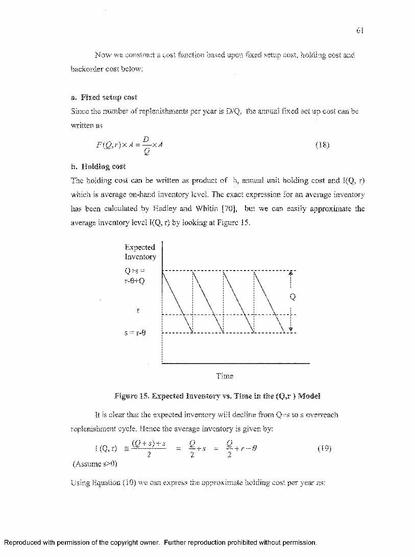
61
Now we construct a cost function based upon fixed setup cost, holding cost and
backorder cost below:
a. Fixed setup cost
Since the number of replenishments per year is D/Q, the annual fixed set up cost can be
written as
F ( Q , r ) x A = ~ - x A (18)
b. Holding cost
The holding cost can be written as product of h, annual unit holding cost and I(Q, r)
which is average on-hand inventory level. The exact expression for an average inventory
has been calculated by Hadley and Whitin [70], but we can easily approximate the
average inventory level I(Q, r) by looking at Figure 15.
Expected Inventory
Q+s = r-O+Q
r
s = r-0
Time
Figure 15. Expected Inventory vs. Time in the (Q,r ) Model
It is clear that the expected inventory will decline from Q+s to s overreach
replenishment cycle. Hence the average inventory is given by:
I (Q, r) E = Q +s = Q + r ^ 0 ( 19)2 2 2
(Assume s>0)
Using Equation (10) we can express the approximate holding cost per year as:
Reproduced with permission of the copyright owner. Further reproduction prohibited without permission.
62
h x I(Q, r) = h(~- + r — 0) (20)
c. Backorder cost;
The number of backorders in a cycle equals the number of backorders on the
books when a replenishment order arrives. If the demand during the replenishment lead
time is x, then the number of backorders can be expressed as
Number of backorders = ^ i f x < rx — r i f x > r
The expected number of backorders that will be placed during a cycle is indicated by n(r)
which is integral of the
n ( r ) = J(x-r)g(x)£& (21)r
Hence the expected number of backorders per year is obtained by multiplying n(r) by the
expected number of cycles per year:
Expected no of backorders per year = B(r) = n(r) (22)
Therefore, total backorder cost will be = h ~ n{r) (23)
Another approach to calculation of quantity B(Q, r) is to compute it similar to fill
rate , by averaging the backorder level for the base stock model over all inventory
positions between r + 1 and r + Q.
I ,+c iB<3,r) = - ' Z m = -[B (r + i)+ ........+ B(r + Q)} (24)
if x=r+l M
To simplify our calculations, we can simply use the base stock backorder formula which
was derived in a previous section in this chapter.
B{Q, r) ~ B(r)
The loss function B (r) which represents the average backorder level in a base stock
model and was shown by Hopp and Spearman [20] to be:
Reproduced with permission of the copyright owner. Further reproduction prohibited without permission.
63
n(r) = 0 pir) + {$ - r)( 1 - G{r)) (25)
Thus, 5 (r) = “ «(/■) j?(r) + (0 - r)(l - G(r))} (26)
Total Cost Formulation
Now substituting in Equation (8), we get the (Q, r) mode! cost function
D ( O ^ Dn a r ) = - A + h f + r - f f + b— n(r) (27)a v 2 ) q
We compute the values of Q and r that minimize this function. Differentiating Y (Q, r)
with respect to Q and setting the result equal to zero yields
*Y(Q,r ) _ - D A + h hDnjr)dQ Q2 2 Q2
This can be simplified as:
DA bDn(r) h 2 D(A + bn(r))—— + ---- AJ- = — or ----- ----- -—— = h and finallye q 2 q
e ^ 2D(A+h bn^ (29)
Now, differentiating Y (Q, r) with respect to r and setting the result equal to zero yields
3 Y ( Q , r) = h + b D M r 1 = 0 (3Q)
dr Q dr
Since
= ^ '°\ix ~ r) s i x)dx = - °°\g(x)dx = - (1 - G(r))
Equation (30) becomes
_ G(r}) = 0 (31)
This can be further simplified and written as equation below:
G(r) = l - M (32)bD
Reproduced with permission of the copyright owner. Further reproduction prohibited without permission.

64
The optimal replenishment quantity Q* and the reorder point r* can be found by
simultaneously solving the following equations (33) and (34):
2 (33)
G(,) = l - § (34)
Since these equations are coupled (i.e., Q depends on r and r depends on Q), we require
an algorithm to solve these.
d. Algorithm for Solving Coupled Equations (Single product (Q, r) model)
Coupled equations like (33) and (34) can be solved by an iterative process which
is described below:
Step 0 Given the known quantities like fixed setup cost A, annual unit holding cost h and
annual demand in units D, we calculate an initial value of order quantity Q0 using
the EOQ model formula.
Then, we find an initial value of reorder point r0 which will satisfy the desired fill
rate calculated by equation (34). This value of r<> is obtained from probability
density function tables that we have already used in base stock model.
Step 1 Then, we compute optimal values for order quantity Q and reorder point r using
equations (33) and (34) which were developed for backorder cost model.
Step 2 In step 2, we compare the results obtained in step 0 and step 1. If the difference
between these values is less than one then these are the optimal values of Q and r.
If the difference is larger than one, we repeat step 1. This is done until the
solutions converge. It is observed that solutions converge quickly, generally
within one or two iterations.
The above algorithm is described here in mathematical form.
Reproduced with permission of the copyright owner. Further reproduction prohibited without permission.
65
Step 0
Set Q0 - and r0 to be the value of r that satisfies
hQ0G(r) = 1 —bD
Let t = 1
Step 1
Compute
q _ \2D(A + bn(rt..,))
h
and compute rt as the value of r that satisfies
M)
Step 2
If |Qt - j < 1 and |rt - rt_x | < 1, stop and set Q* = Qt, r* = rt. Otherwise, set
t ~ t + \ and go to step (1).
This algorithm generally converges quickly.
e, Basic (Q, r) Insights
The basic insights behind the (Q, r) model are essentially those of EOQ and base
stock model namely:
• Cycle stock increases as replenishment frequency decreases
• Safety stock provides a buffer against stockouts
(Q, r) model and base stock models ( same a (Q, r) mode! except Q = 1) are
historically early attempts to explicitly model variability in the supply chain and provide
quantitative understanding of how safety stock affects the customer service level. This
model suggests that the safety stock, service level and backorder levels are primarily
affected by the reorder point r, while cycle stock and order frequency are essentially
functions of order quantity Q.
Reproduced with permission of the copyright owner. Further reproduction prohibited without permission.
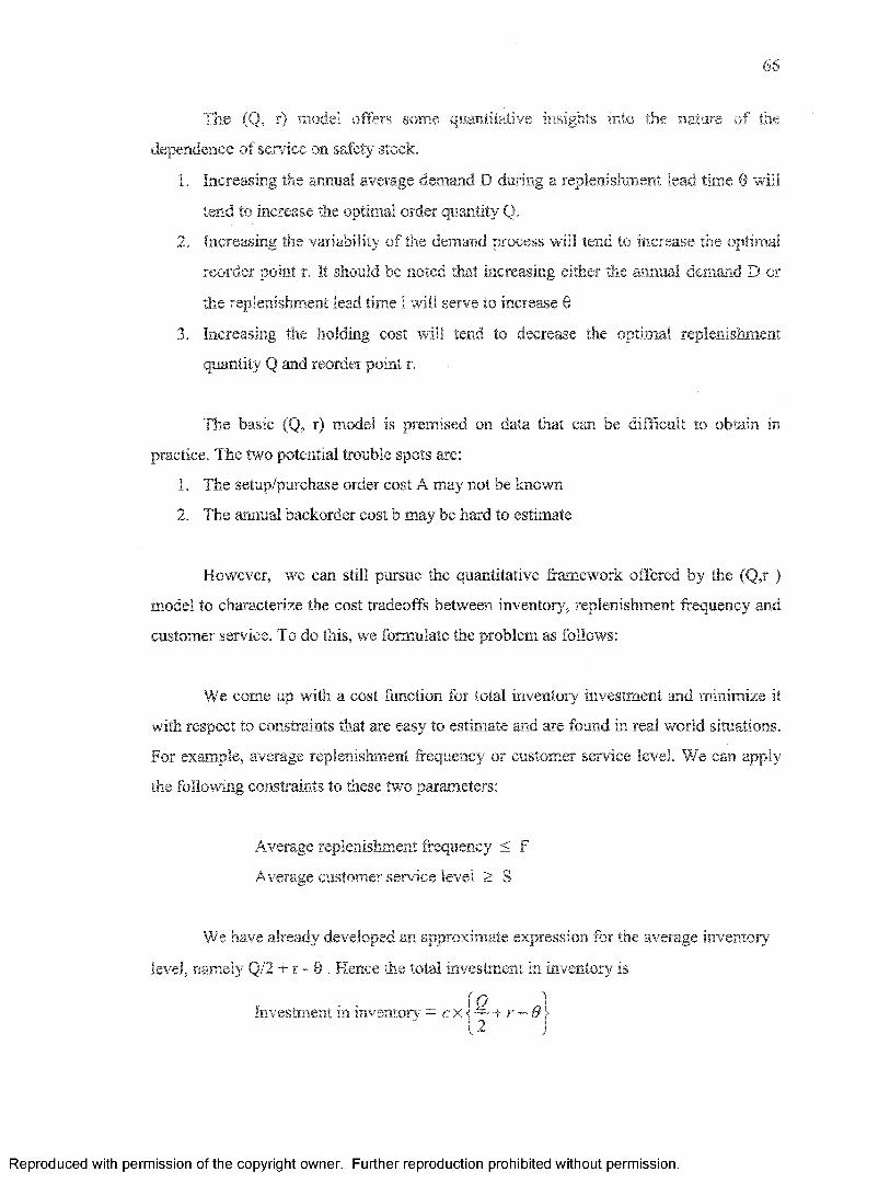
66
The (Q, r) model offers some quantitative insights into the nature of the
dependence of sendee on safety stock.
1. Increasing the annual average demand D during a replenishment lead time 8 will
tend to increase the optimal order quantity Q.
2. Increasing the variability of the demand process will tend to increase the optimal
reorder point r. It should be noted that increasing either the annual demand D or
the replenishment lead time 1 will serve to increase 0
3. Increasing the holding cost will tend to decrease the optimal replenishment
quantity Q and reorder point r.
The basic (Q, r) model is premised on data that can be difficult to obtain in
practice. The two potential trouble spots are:
1. The setup/purchase order cost A may not be known
2. The annual backorder cost b may be hard to estimate
However, we can still pursue the quantitative framework offered by the (Q,r )
model to characterize the cost tradeoffs between inventory, replenishment frequency and
customer service. To do this, we formulate the problem as follows:
We come up with a cost function for total inventory investment and minimize it
with respect to constraints that are easy to estimate and are found in real world situations.
For example, average replenishment frequency or customer service level. We can apply
the following constraints to these two parameters:
Average replenishment frequency < F
Average customer service level > S
We have already developed an approximate expression for the average inventory
level, namely Q/2 + r - 0 . Hence the total investment in inventory is
Investment in inventory = c x t — + r - 9I 2 j
Reproduced with permission of the copyright owner. Further reproduction prohibited without permission.

67
The customer service or fill rate is given by
Fill rate = 1 - ^Q
Hence, from the above discussion we can formulate the problem as follows:
Min c x i — + r - 0 \ Subject to: — < F and 1 - > S12 J Q Q
After solving these equations we can rationally balance the frequency of
replenishment and customer sendee with inventory investment.
5.6 Application of (Q, r) Model - An Example
We consider the example of an appliance store that sells various models of
refrigerators. We know from past experiences that the mean demand for a certain model
is 14 units per year, and replenishment lead time is 45 days. This example was adapted
from a book by Hoop and Spearman [20] and included here to illustrate the application of
this model.
Annual demand is D = 14 units/year
Unit cost of the part = $150
Annual holding cost, h = $15
Replenishment lead time, 1 = 45 days
Average demand during a replenishment lead time is
D 146 = x / = ----- x45 = 1.726
365 365
The cost of each backorder, b = $ 40
Let us model the demand using Poisson distribution.
0 re~e W e ~ wp(r) = Probability {Demand during lead time = r } = ------- = ----------
r\ r Sr i \ Q r e ~ l °
And G (r) Cumulative Probability Distribution = T"' p(r) = Y ---------r\
Number of backorders in a replenishment cycle, n(r) = 0 p(r) + (&- ?-)(! - G(r)}
Reproduced with permission of the copyright owner. Further reproduction prohibited without permission.
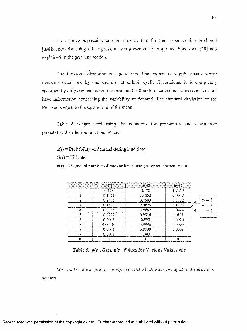
68
This above expression n(r) is same as that for the base stock model and
justification for using this expression was presented by Bopp and Spearman [20] and
explained in the previous section.
The Poisson distribution is a good modeling choice for supply chains where
demands occur one by one and do not exhibit cyclic fluctuations. It is completely
specified by only one parameter, the mean and is therefore convenient when one does not
have information concerning the variability of demand. The standard deviation of the
Poisson is equal to the square root of the mean.
Table 6 is generated using the equations for probability and cumulative
probability distribution function. Where:
p(r) = Probability of demand during lead time
G(r) = Fill rate
n(r) - Expected number of backorders during a replenishment cycle
r . .. pin r^ E i: m .r)0 0.178 0.178 1 1.7260i 0.3072 0.4852 0.90402 0.2651 0.7503 0.38923 0.1525 0.9029 0.13964 0.0658 0.9687 0.04245 0.0227 0.9914 0.01116 0.0065 0.998 0.00267 0.00016 0.9996 0.00058 0.0003 0.9999 0.0001
[ 9 0.0001 1.000 110 0 1 0
( n\ n Tr0= 3
3
Table 6, p(r), G(r), n(r) Values for Various Values of r
We now test the algorithm for (Q, r) model which was developed in the previous
section.
Reproduced with permission of the copyright owner. Further reproduction prohibited without permission.
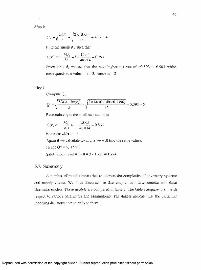
69
Step 0
J2AD ( 2 X 1 0 X 1 4
& V A 1 15
Find the smallest r such that
G(r) > 1 - = 1 - = 0,893bD 40x14
From table 6, we see that the next higher fill rate afterO.893 is 0.903 which
corresponds to a value of r = 3. Hence tq- 3
Step 1
Compute Qj
Q ^ J 2D(A + b n ( r j = ^2x14(10 + 40x 013967 = ; ^ ^ g
Recalculate ri as the smallest r such that
G( r ) > 1_ t a = 1 _ i 5 x i =0 866bD 40x14
From the table x\ = 3
Again if we calculate Q2 and 12 we will find the same values.
Hence Q* = 5, r* = 3
Safety stock level = r - 0 = 3 - l .726 = 1.274
5.7. Summary
A number of models have tried to address the complexity of inventory systems
and supply chains. We have discussed in this chapter two deterministic and three
stochastic models. These models are compared in table 7. The table compares them with
respect to various parameters and assumptions. The dashes indicate that the particular
modeling decisions do not apply to them.
Reproduced with permission of the copyright owner. Further reproduction prohibited without permission.
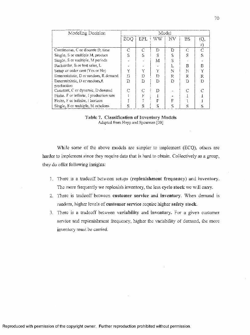
70
Modeling Decision ModelEOQ EPL WW NY BS (Q>
r)Continuous, C or discrete D, time C C D D c CSingle, S or multiple M, product s s S s s sSingle, S of multiple, M periods _ - M S . .
Backorder, B or lost sales, L . - - L B BSetup or order cost (Yes or No) Y Y Y N N YDeterministic, D or random, R demand D D D R R RDeterministic, D or random,R D D D D D DproductionConstant, C or dynamic, D demand C C D C CFinite, F or infinite, I production rate I F I - I IFinite, F or infinite, I horizon I I F F I ISingle, S or multiple, M echelons s S S S S s
Table 7. Classification of Inventory ModelsAdapted from Hopp and Spearman [20]
While some of the above models are simpler to implement (ECQ), others are
harder to implement since they require data that is hard to obtain. Collectively as a group,
they do offer following insights:
1. There is a tradeoff between setups (replenishment frequency) and inventory.
The more frequently we replenish inventory, the less cycle stock we will carry.
2. There is tradeoff between customer service and inventory. When demand is
random, higher levels of customer service require higher safety stock.
3. There is a tradeoff between variability and inventory. For a given customer
service and replenishment frequency, higher the variability of demand, the more
inventory must be carried.
Reproduced with permission of the copyright owner. Further reproduction prohibited without permission.

71
Chapter - 6
APPLICATION OF BASE STOCK MODEL
In this chapter, we apply the base stock model to a serial three level multiechelon
single product supply chain system as shown in Figure 16. Supply chain systems like
these are very common in industry. Research literature includes several examples of two
level supply chains. Hopp and Spearman [20] discuss a two level arborescent system. It is
important to study this since, supply chain dynamics effects like builwhip effect get more
amplified in a three level serial system.
Decision Variable = Reorder Point Inventory- rFill rate = 0.9, Poisson distribution for demand, Vary replenishment lead time
Secondary Soapier (engine
part) r -?
*PrimarySupplier(Engine) .
r * ?m l
:
Warehouse ] : k (HSngtae) ' f ;
f :
Customer(Engine)
Demand « Cons.
Step - 3 Step - J‘hep - I
Figure 16. Base Stock Model Applied to Three Level Serial Supply Chain
Our goal is to study these supply chains by applying base stock (chapter 6) and
(Q, r) models (chapter 7) and compare the results. We then, study these systems using
physical simulations and validate the findings of mathematical models through physical
simulations. Finally we, validate these models through the use of a computer based
simulation model using ProModel software.
In this section we evaluate base stock model for five replenishment lead time, 12,
8, 6, 4, and 2 months and calculate reorder point for these cases. We start with the bottom
of the supply chain and based upon customer demand calculate the inventory level that
must be kept at the warehouse for a given fill rate (Step - 1 in Figure 16). For all these
cases, the desirable fill rate is assumed to be 90%. Then, we move up the supply chain
and calculate the quantity that must be stored at primary supplier to attain desired fill rate
Reproduced with permission of the copyright owner. Further reproduction prohibited without permission.

72
for orders received from the warehouse (Step - 2 in Figure 16). This is repeated until we
have the r values for each entity in the supply chain.
Cost Analysis:
We can formulate the quantitative cost analysis by first looking at the expression
for average inventory level. For most of the cases, unless there is seasonal product
demand, the average inventory position can be expressed as:
Inventory Position = Average Inventory + Safety Stock
Average Inventory = Q/2
Safety Stock = s = r - 0
We will use these cost equations to compare the various cases later in chapter 6.
The following pages include the analysis for five replenishment lead times.
Therefore: Inventory Position = - + r - 9 > and
Investment in inventory = c x | — v r - 6
Where c = unit cost of product in dollars
Total Cost = Order Cost + c x
Reproduced with permission of the copyright owner. Further reproduction prohibited without permission.

73
6,1 Replenishment Lead Time = 12 months
Customer (Engine)
Demand =10
Warehouse (Engine)
r = 14
Primary Supplier (Engine)
r =19
SecondarySupplier
(engine parts) r =25
Location - Warehouse
Average Demand = 10 units per year
Replenishment lead time, 1=12 months
Average demand during replenishment lead time, 0 = j-xlO = 10 units
We model the demand based upon Poisson distribution:
6 re~8 10re“'°p(r) = Probability {Demand during lead time = r} = --------= ----------
rl r\
And G (r) Cumulative Probability Distribution = ^ p(k ) = ^ ---------A= 0 *=0
The Poisson distribution is a good modeling choice for supply chains where
demands occur one by one and do not exhibit cyclic fluctuations. It is completely
specified by only one parameter, the mean and is therefore convenient when one does not
have information concerning the variability of demand. The standard deviation of the
Poisson is equal to the square root of the mean.
Reproduced with permission of the copyright owner. Further reproduction prohibited without permission.

74
< = p i *
Table 8. Fill Rates for Various Values of r, 1 =12 months
For a fill rate of 90% { G(r) > 0.9}, we get a value of r = 14 from Table 8. Which
means, at least 14 units must be stored at the warehouse to get a fill rate of 90%.
Location - Prim ary Supplier
Average Demand is 14 units per year from the ware house. We calculate the
quantity that must be stored by the primary supplier to meet a fill rate of 90%, by
constructing the table below for the demand that follows a Poisson distribution.
0 0.00 0.00 10.00i 0.00 0.00 9.002 0.00 0.00 8.003 0.01 0.01 7.004 0.02 0.03 6.015 0.04 0.07 5.046 0.06 0.13 4.117 0,09 0.22 3.248 0.11 0.33 2.469 0.13 0.46 1.7910 0.13 0.58 1.2511 0.11 0.70 0.8312 0.09 0.79 0.5313 0.07 0.86 0.3214 0.05 0.92 0.1915 0.03 0.95 0.1016 0.02 0.97 0.0517 0.01 0.99 0.0318 0.01 0.99 0.01
Reproduced with permission of the copyright owner. Further reproduction prohibited without permission.

75
i r p( r ) (Hr J1 0.00 0.002 0.00 0.003 0.00 0.004 0.00 0.005 0.00 0.016 0.01 0.017 0.02 0.038 0.03 0.069 0.05 0.11to 0.07 0.1811 0.08 0.2612 0.10 0.3613 0.11 0.4614 0.11 0.5715 0.10 0.6716 0.09 0.7617 0.07 0.8318 0.06 0.8819 0.04 0.9220 0.03 0.9521 0.02 0.9722 0.01 0.9823 0.01 0.99
Table 9. Fill Rates for Various Values of r, 1 = 12 months
In order to maintain the fill rate of 90%, we need r =19 at primary supplier
Thus, safety stock =19-14 = 5
Location - Secondary Supplier
Average demand is 19 units per year from the primary supplier. We calculate the quantity
that must be stored by the secondary supplier to meet a fill rate of 90%, by constructing
the table below for the demand that follows a Poisson distribution.
Reproduced with permission of the copyright owner. Further reproduction prohibited without permission.
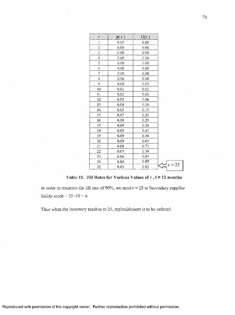
76
1 0.00 0.002 0.00 0.003 0.00 0.004 0.00 0.005 0.00 0.006 0.00 0.007 0.00 0.008 0.00 0.009 0.00 0.0110 0.01 0.0211 1 0.02 0.0312 0.03 0.0613 0.04 0.1014 0.05 0.1515 0.07 0.2116 0.08 0.2917 0.09 0.3818 0.09 0.4719 0.09 0.5620 0.09 0.6521 0.08 0.7322 0.07 0.7923 0.06 0.8524 0.04 0.8925 0.03 0.93
Table 10. Fill Mates for Various Values of r , 1 = 12 months
In order to maintain the fill rate of 90%, we need r = 25 at Secondary supplier
Safety stock = 25 -19 = 6
Thus when the inventory reaches to 25, replenishment is to be ordered.
Reproduced with permission of the copyright owner. Further reproduction prohibited without permission.
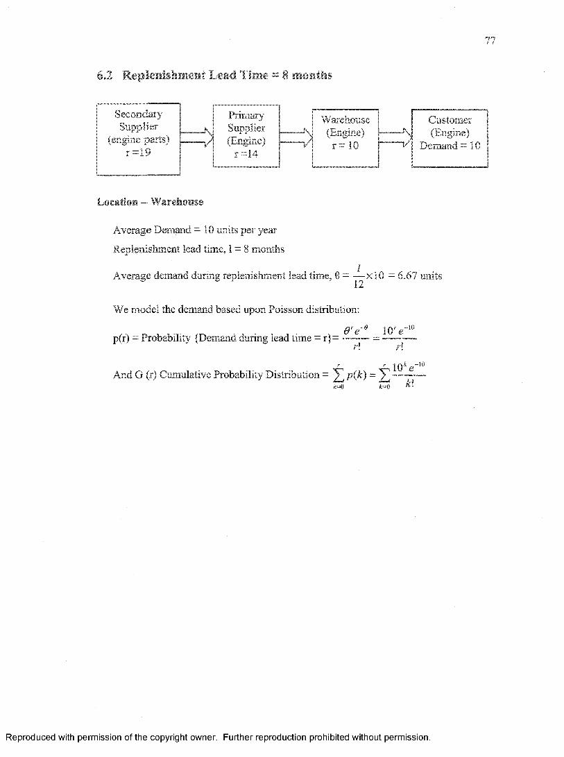
77
6.2 Replenishment Lead Time = 8 months
SecondarySupplier
(engine parts)r =19
Y (Engine) r =14
Primary jy Supplier
|
Warehouse (Engine)
r = 10
Customer (Engine)
Demand =10
Location — Warehouse
Average Demand = 10 units per year
Replenishment lead time, 1 = 8 months
Average demand during replenishment lead time, 0 = ~ x 10 = 6.67 units
We model the demand based upon Poisson distribution:
0 re~e 10W”10p(r) = Probability {Demand during lead time = r} = --------= ----------
r\ r\r r 1 f \ k „ - 1 0
And G (r) Cumulative Probability Distribution = —
Reproduced with permission of the copyright owner. Further reproduction prohibited without permission.

78
fr
0p ( r ) 0.00
t If *■ $
0.00 1.671 0.01 0.01 5.672 0.03 0.04 4.693 0.06 0.10 3.724 0.10 0.21 2.825 0.14 0.34 2.026 0.16 0.50 1.377 0.15 0.65 0.878 0.12 0.77 0.529 0.09 0.86 0.29
10 0.06 0.92 0.1511 0.04 0.96 0.0712 0.02 0.98 0.0313 0.01 0.99 0.0114 0.01 1.00 0.0115 0.00 1.00 0.00
Table 11. Fill Rates for Various Values of r, 1 = 8 months
Let the customer has average demand of 6.67 units (say engine).
For fill rate of 90% and referring Table 11
r = 10 units per 8 months to be stocked at warehouse.
Location - Primary Supplier
Average Demand = 10 units per 8 months We calculate the quantity that must be stored
by the primary supplier to meet a fill rate of 90%, by constructing the table below for the
demand that follows a Poisson distribution.
Reproduced with permission of the copyright owner. Further reproduction prohibited without permission.

79
r ...... Hr)...... i t l r )1 0.00 0.002 0.00 0.003 0.01 0.014 0.02 0.035 0.04 0.076 0.06 0.137 0.09 0.228 0.11 0.339 0.13 0.4610 0.13 0.5811 0.11 0.7012 0.09 0.7913 0.07 0.8614 0.05 0.9215 0.03 0.9516 0.02 0.9717 0.01 0.9918 0.01 0.99
14
Table 12. Fill Rates for Various Values of r, I = 8 months
In order to maintain the f ill rate of 90%, we need r = 1 4 at Primary supplier
Safety stock = 14-10 = 4
Reproduced with permission of the copyright owner. Further reproduction prohibited without permission.
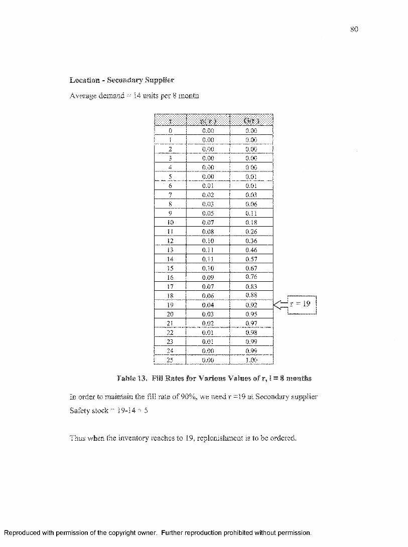
80
Location - Secondary Supplier
Average demand = 14 units per 8 month
......i l l ' * ...... 1A ;0 0.00 0.001 0.00 0.002 0.00 0.003 0.00 0.004 0.00 0.005 0.00 0.016 0.01 0.017 0.02 0.038 0.03 0.069 0.05 0.1110 0.07 0.1811 0.08 0.2612 0.10 0.3613 0.11 0.4614 0.11 0.5715 0.10 0.6716 0.09 0.7617 0.07 0.8318 0.06 0.8819 0.04 0.9220 0.03 0.9521 0.02 0.9722 0.01 0.9823 0.01 0.9924 0.00 0.9925 0.00 1.00
Table 13. Fill Rates for Various Values of r, 1 = 8 months
In order to maintain the fill rate of 90%, we need r =19 at Secondary supplier
Safety stock =19-14 = 5
Thus when the inventory reaches to 19, replenishment is to be ordered.
Reproduced with permission of the copyright owner. Further reproduction prohibited without permission.
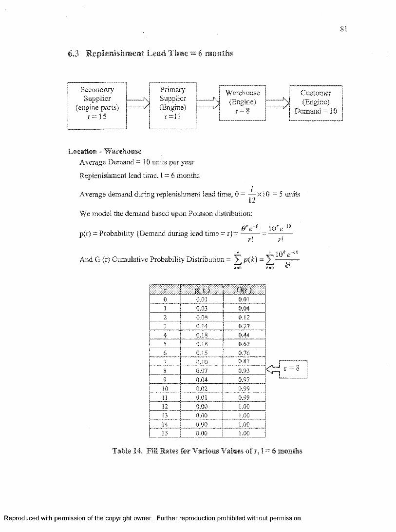
81
6.3 Replenishment Lead Time = 6 months
Secondary Primary |Supplier — — \ i Supplier j-
(engine parts) h----- (Engine) J~r= 15 r =11 |
I
Warehouse| (Engine)| r = 8
Customer
Demand = 10
Location - WarehouseAverage Demand =10 units per year
Replenishment lead time, 1 = 6 months
Average demand during replenishment lead time, 0 = -^-xlO = 5 units
We model the demand based upon Poisson distribution:
6 re e 1 0 'A 10p(r) = Probability {Demand during lead time = r}=r\ r\
k -10r r ^And G (r) Cumulative Probability Distribution = p(k) = ^ — —
jfc=0 k=0
iy j t A'' 0 0.01
G(r)0.01
l 0.03 0.042 0.08 0.123 0.14 0.274 0.18 0.445 0.18 0.626 0.15 0.767 0.10 0.87
8 0.07 0.939 0.04 0.9710 0.02 0.9911 0.01 0.9912 0.00 1.0013 0.00 1.0014 0.00 1.0015 0.00 1.00
^\ r i
Table 14. Fill Rates for Various Values of r, 1 = 6 months
Reproduced with permission of the copyright owner. Further reproduction prohibited without permission.
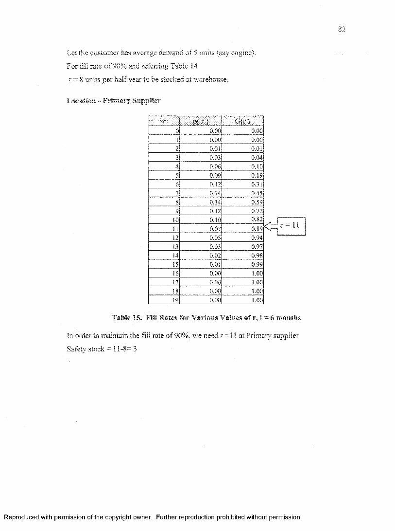
82
Let the customer has average demand of 5 units (say engine).
For fill rate of 90% and referring Table 14
r = 8 'units per half year to be stocked at warehouse.
Location - Primary Supplier
r p i 1 ) G (r)0 0.00 0.00
i 0.00 0.002 0.01 0.013 0.03 0.044 0.06 0.105 0.09 0.196 0.12 0.31
7 0.14 0.458 0.14 0.599 0.12 0.72
10 0.10 0.82
I t 0.07 0.8912 0.05 0.9413 0.03 0.9714 0.02 0.9815 0.01 0.9916 0.00 1.0017 0.00 1.0018 0.00 1.0019 0.00 1.00
Table 15. Fill Rates for Various Values of r, 1 = 6 months
In order to maintain the fill rate of 90%, we need r =11 at Primary supplier
Safety stock = 11-8= 3
Reproduced with permission of the copyright owner. Further reproduction prohibited without permission.

83
Location - Secondary Supplier
0G(.i ) 0.00
1 0.00 0.002 0.00 0.003 0.00 0.004 0.01 0.025 0.02 0.046 0.04 0.087 0.06 0.148 0.09 0.239 0.11 0.3410 0.12 0.4611 0.12 0.5812 0.11 0.6913 0.09 0.7814 0.07 0.85
15 0.05 0.9116 0.04 0.9417 0.02 0.9718 0.01 0.9819 0.01 0.9920 0.00 1.00
15
Table 16. Fill Rates for Various Values of r, 1 = 6 months
In order to maintain the fill rate of 90%, we need r =15 at Secondary supplier
Safety stock = 15-11=4
Thus when the inventory reaches to 11, replenishment is to be ordered.
Reproduced with permission of the copyright owner. Further reproduction prohibited without permission.

84
6.4 Replenishment Lead Time = 4 months
Customer (Engine)
Demand = 10
Warehouse(Engine)
PrimarySupplier (Engine)
r = 9
SecondarySupplier
(engine parts)
Location - Warehouse
Average Demand = 10 units per year
Replenishment lead time, 1 = 4 months
Average demand during replenishment lead time, 0 = ~ x 10 = 3.33 units
We model the demand based upon Poisson distribution:
0 re~e 10re“10p(r) = Probability (Demand during lead time = r} = ------- = ----------
r! r!r ' r JQ*
And G (r) Cumulative Probability Distribution = ^ p ( k ) = ----------k=0 4=0
Reproduced with permission of the copyright owner. Further reproduction prohibited without permission.
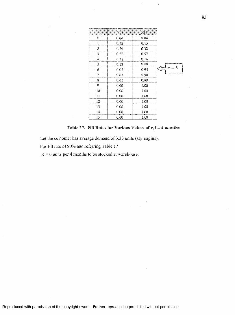
85
r . ,, 0
p ff)0.04 0.04
1 0.12 0.152 0.20 0.323 0.22 0.574 0.18 0.765 0.12 0.88
6 0.0 / 0.957 0.03 0.988 0.01 0.999 0.00 1.0010 0.00 1.0011 0.00 1.0012 0.00 1.0013 0.00 1.0014 0.00 1.0015 0.00 1.00
Table 17. Fill Rates for Various Values of r, 1 = 4 months
Let the customer has average demand of 3.33 units (say engine).
For fill rate of 90% and referring Table 17
R = 6 units per 4 months to be stocked at warehouse.
Reproduced with permission of the copyright owner. Further reproduction prohibited without permission.

86
Location - Primary Suppler
Average Demand =6 units per 4jmonthsr ru t Off?0 0.00 0.001 0.01 0.022 0.04 0.063 0.09 0.154 0.13 0.295 0.16 0.456 0.16 0.617 0.14 0.748 0.10 0.859 0.07 0.9210 0.04 0.9611 0.02 0.9812 0.01 0.9913 0.01 1.0014 0.00 1.0015 0.00 1.0016 0.00 1.00
Table 18. Fill Rates for Various Values of r, 1 = 4 months
In order to maintain the fill rate of 90%, we need r = 9 at Primary supplier Safety stock = 9-6 = 3 units
Reproduced with permission of the copyright owner. Further reproduction prohibited without permission.
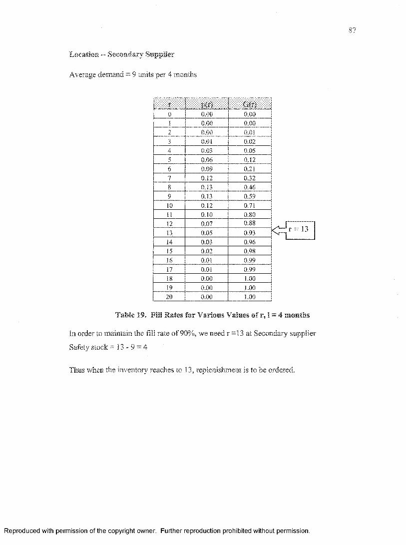
87
Location - Secondary Supplier
Average demand = 9 units per 4 months
ir . .' .: t i t )0 0.00 0.001 0.00 0.002 0.00 0 .013 0.01 0.024 0.03 0.055 0.06 0.126 0.09 0.217 0.12 0.328 0.13 0.469 0.13 0.5910 0.12 0.7111 0.10 0.8012 0.07 0.8813 0.05 0.9314 0.03 0.9615 0.02 0.9816 0.01 0.9917 0.01 0.9918 0.00 1.0019 0.00 1.0020 0.00 1.00
Table 19. Fill Rates for Various Values of r, 1 = 4 months
In order to maintain the fill rate of 90%, we need r =13 at Secondary supplier
Safety stock = 1 3 - 9 = 4
Thus when the inventory reaches to 13, replenishment is to be ordered.
Reproduced with permission of the copyright owner. Further reproduction prohibited without permission.

88
6.5 Replenishment Lead Time = 2 months
SecondarySupplier
(engine parts) r = 8
V (Engine) r = 5
SupplierPrimary
> / (Engine) r = 3
Warehouse^ (Engine)
Demand =10
Customer
Location - Warehouse
Average Demand = 10 units per year
Replenishment lead time, 1 = 2 months
Average demand during replenishment lead time, 0 = ^ x l G = 1.67 units
We model the demand based upon Poisson distribution:
6 Te~° W e~wp(r) = Probability {Demand during lead time = r} = ------- = ----------rl rl
r r
And G (r) Cumulative Probability Distribution = ^ p ( k ) = ^k =0 4=0
Reproduced with permission of the copyright owner. Further reproduction prohibited without permission.

89
: , P l O0 0.19 0.19i 0.31 0.502 0.26 0.583 0.15 0.914 0.06 0.975 0.02 0.996 0.01 1.007 0.00 1.003 0.00 1.009 0.00 1.0010 0.00 1.0011 0.00 1.0012 0.00 1.0013 0.00 1.0014 0.00 1.0015 0.00 1.00
— t = 3^—L
Table 20. Fill Rates for various values of r, 1 = 2 months
Let the customer has average demand of 1.67 units (say engine). For fill rate of 90% and referring Table 20 r = 3 units per 2 months to be stocked at warehouse.
Reproduced with permission of the copyright owner. Further reproduction prohibited without permission.
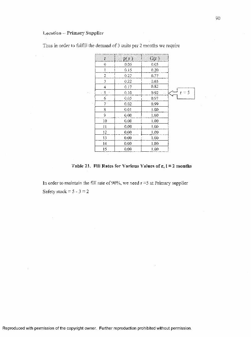
Location — Prim ary Supplier
Thus in order to fulfill the demand of 3 units per 2 months we require
r H r ) ( l ( T )0 0.05 0.051 0.15 0.202 0.22 0.373 0.22 0.654 0.17 0.82
5 0.10 0.926 0.05 0.977 0.02 0.998 0.01 1.009 0.00 1.0010 0.00 1.0011 0.00 1.0012 0.00 1.0013 0.00 1.0014 0.00 1.0015 0.00 1.00
Table 21. Fill Rates for Various Values of r, 1 = 2 months
In order to maintain the fill rate of 90%, we need r =5 at Primary supplier
Safety stock = 5 - 3 = 2
Reproduced with permission of the copyright owner. Further reproduction prohibited without permission.
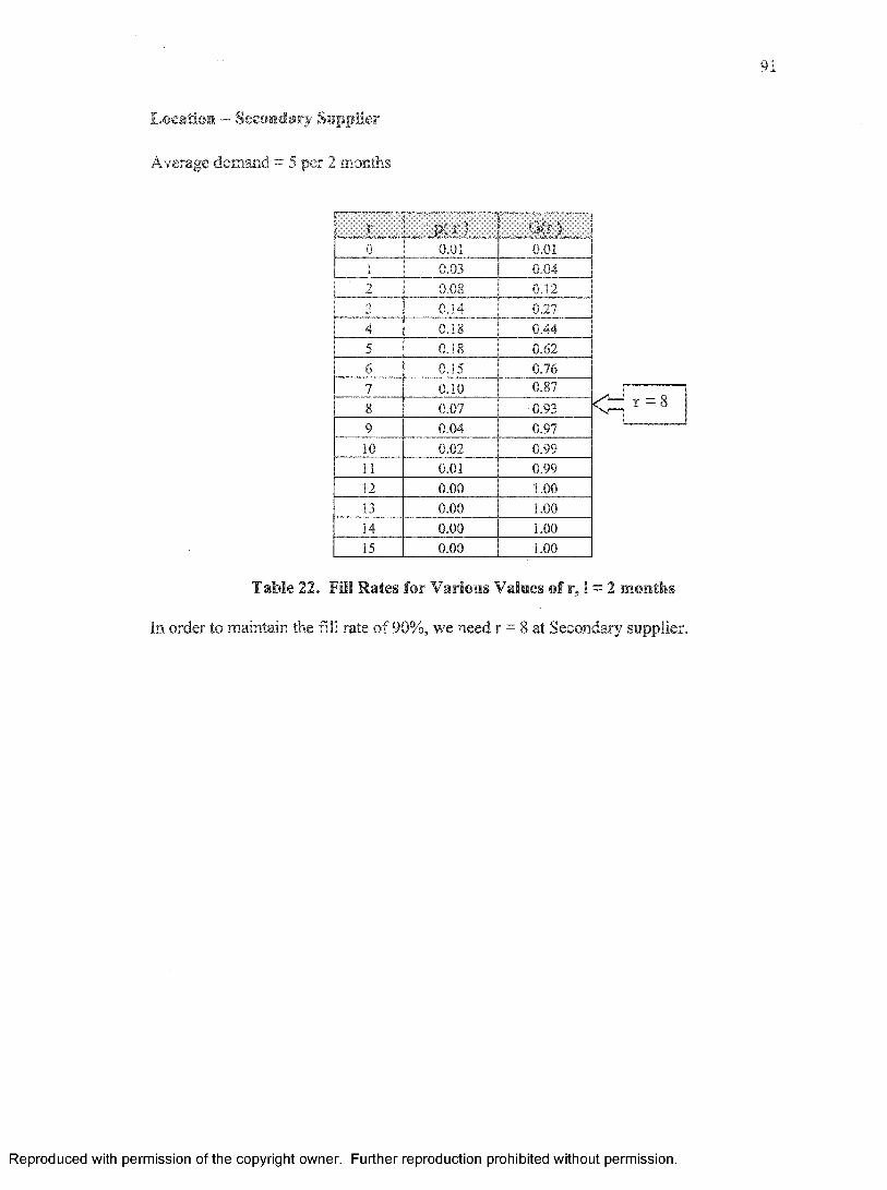
91
Location — Secondary Supplier
Average demand = 5 per 2 months
0 0.01___ Q ( f )
0.01! ^ 0.03 0.042 0.08 0.123 0.14 0.274 0.18 0.445 0.18 0.626 0.15 0.767 0.10 0.878 0.07 0.939 0.04 0.9710 0.02 0.9911 0.01 0.9912 0.00 1.0013 0.00 1.0014 0.00 1.0015 0.00 1.00
Table 22. Fill Rates for Various Values of r, I = 2 months
In order to maintain the fill rate of 90%, we need r = 8 at Secondary supplier.
Reproduced with permission of the copyright owner. Further reproduction prohibited without permission.
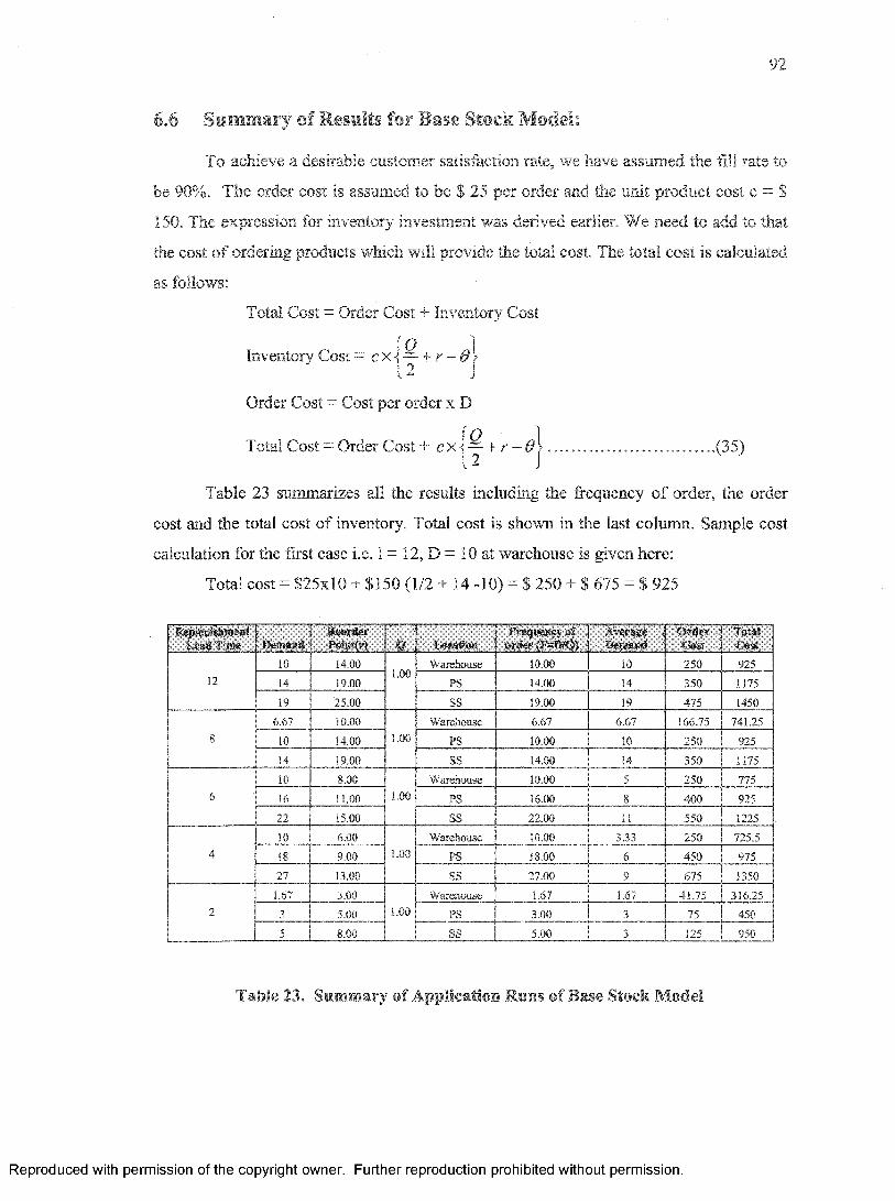
92
£6 Summary of Results for Base Stock Model:
To achieve a desirable customer satisfaction rate, we have assumed the fill rate to
be 90%. The order cost is assumed to be $ 25 per order and the unit product cost c = $
150. The expression for inventory investment was derived earlier. We need to add to that
the cost of ordering products which will provide the total cost. The total cost is calculated
as follows:
Total Cost = Order Cost + Inventory Cost
Inventory Cost = cx j-y + r - $ j
Order Cost = Cost per order x D
Total Cost = Order Cost + cx + r - ^ | ................... (35)
Table 23 summarizes all the results including the frequency of order, the order
cost and the total cost of inventory. Total cost is shown in the last column. Sample cost
calculation for the first case i.e. 1 = 12, D = 10 at warehouse is given here:
Total cost = $25x10 + $150 (1/2 + 14 -10) = $ 250 + $ 675 = $ 925
RepleaislHweB? ' ' :.: Ocmaj*d Pwittt(r) p . .. — ‘
AverageDemand
Ov" TotalVm i
1210 14.00
1.00Warehouse 10.00 10 250 925
14 19.00 PS 14.00 14 350 317519 25.00 SS 19.00 19 475 1450
86.67 10.00
1.00Warehouse 6.67 6.67 166.75 741.25
10 14.00 PS 10.00 10 250 92514 19.00 SS 14.00 14 350 1175
610 8.00
1.00Warehouse 10.00 5 250 775
16 11.00 PS 16.00 8 400 92522 15.00 SS 22.00 11 550 1225
410 6.00
1.00Warehouse 10.00 3.33 250 725.5
18 9.00 PS 18.00 6 450 97527 13.00 SS 27.00 9 675 1350
21.67 3.00
1.00Warehouse 1.67 1.67 41.75 316.25
3 5.00 PS 3.00 3 75 4505 8.00 SS 5.00 3 125 950
Table 23. Summary of Application Runs of Base Stock Model
Reproduced with permission of the copyright owner. Further reproduction prohibited without permission.
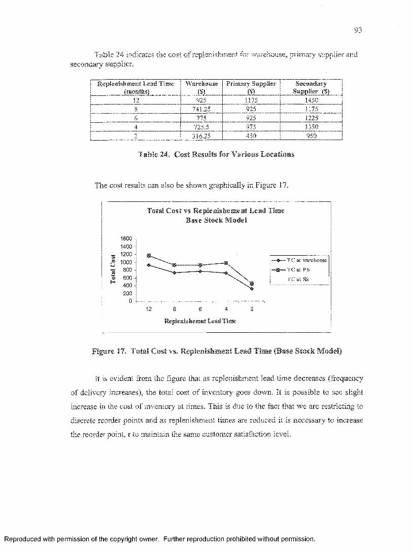
93
Table 24 indicates the cost of replenishment for warehouse, primary supplier and secondary supplier.
Replenishment Lead Time (months)
Warehouse(S)
Primary Supplier ($1
Secondary 1 Supplier ($)
12 925 1175 1450 18 741.25 925 1175 |6 775 925 1225 I-
725.5 975 1350 I2 316.25 450 950 |
Table 24. Cost Results for Various Locations
The cost results can also be shown graphically in Figure 17.
Total Cost vs Meplenlshement Lead Time Base Stock Model
■aeU$oH
1600 1400 1200 1000 800 600 400 -I 200
0
—♦— TC at warehouse
TC at PS
TC at SS
12 8 6 4
Replenishemnt Lead Time
Figure 17. Total Cost vs. Replenishment Lead Time (Base Stock Model)
It is evident from the figure that as replenishment lead time decreases (frequency
of delivery increases), the total cost of inventory goes down. It is possible to see slight
increase in the cost of inventory at times. This is due to the fact that we are restricting to
discrete reorder points and as replenishment times are reduced it is necessary to increase
the reorder point, r to maintain the same customer satisfaction level.
Reproduced with permission of the copyright owner. Further reproduction prohibited without permission.

94
Reorder Point vs Replenishment Lead Time Base Stock Model
r at warehouse \I
12 8 6 4
Replenishment Lead Time
2
Figure 18. Reorder Point vs. Replenishment Lead Time (Base Stock Model)
Figure 18 shows the plot of reorder point at Warehouse, Primary Supplier and
secondary supplier when Base Stock model is used for inventory control with different
replenishment lead-time. We can see from Figure 18 that the reorder point decreases with
reduction in replenishment lead time. This also leads to reduction in total cost as
frequency of replenishment is increased.
Reproduced with permission of the copyright owner. Further reproduction prohibited without permission.

95
Chapter - 7
APPLICATION OF (Q, r) MODEL
In this chapter, we apply the (Q, r) mode! to a serial three level multiechelon
single product supply chain system as shown in Figure 19, Supply chain systems like
these are very common in industry. Research literature includes several examples of two
level supply chains. Hopp and Spearman [20] discuss a two level arborescent system. It is
important to study this since supply chain dynamics effects like bullwhip effect get more
amplified in a three level serial system.
Decision Variables = Order Quantity, Q and Reorder Point Inventory- r Fill rate = 0.9, Poisson distribution for demand, Vary replenishment lead time
Secondary Supplier (engine
part)Qandr = ?
• 3
. P rfw rySupplier (— t(Engine)
Q and r * ? , |
Warehouse(iBgtH#
Qaitdr = ‘?
Customer (Engine)
Demand -*■ Cons.
Step ■Figure 19. (Q, r) Model Applied to Three Level Serial Supply Chain
Our goal is to study these supply chains by applying base stock (chapter 6) and
(Q, r) models (chapter 7) and compare the results. We then, study these systems using
physical simulations and validate the findings of mathematical models through physical
simulations. Finally, we validate these models through the use of a computer based
simulation model using ProModel software.
In this section we evaluate base stock model for five replenishment lead time, 12,
8, 6, 4, and 2 months and calculate reorder point for these cases. We start with the bottom
of the supply chain and based upon customer demand calculate the inventory level that
must be kept at the warehouse for a given fill rate (Step - 1 in Figure 19). For all these
cases, the desirable fill rate is assumed to be 90%. Then, we move up the supply chain
and calculate the quantity that must be stored at primary supplier to attain desired fill rate
Reproduced with permission of the copyright owner. Further reproduction prohibited without permission.
96
for orders received from the warehouse (Step - 2 in Figure 19), This is repeated until we
have the r values for each entity in the supply chain.
Cost Analysis:
We can formulate the quantitative cost analysis by first looking at the expression
for average inventory level. For most of the cases, unless there is seasonal product
demand, the average inventory position can be expressed as:
Inventory Position = Average Inventory + Safety Stock
Average Inventory = Q/2
Safety Stock = s = r - 0
Where c = unit cost of product in dollars
We will use these cost equations to compare the various cases later in the chapter.
Therefore: Inventory Position = + r - 6 \ and
Investment in inventory = cx< — + r - 0
Reproduced with permission of the copyright owner. Further reproduction prohibited without permission.

97
7.1 Replenishment Lead Time = 12 months
Secondary Primary Warehouse CustomerSupplier |
(engine parts) LSupplier(Engine) — J \ (Engine)
r= 13 z z d )(Engine)
Demand = 10t = 20 r = 16 Q - 5 units /year0 = 7 | 0 = 7
Location - Warehouse
Replenishment Lead time =12 months
Annual demand is D = 10 units/year
Unit cost of the part = $150
Annual holding cost h = $ 15
Average demand during a replenishment lead time is
0 = -----— x l = — xl 2 = 10 units12 months 12
The cost of stockout = b = $40
We model the demand based upon Poisson distribution:
6 7e e 1 0 r e~10p(r) = Probability {Demand during lead time = r}=r l r l
? I0ke~wAnd G (r) Cumulative Probability Distribution = / ^ p { k ) = 2u— —
k —0 &=0
Number of backorders in a replenishment cycle, n(r) = 6 p(r) + (0 - r ) ( l - G(r))
Reproduced with permission of the copyright owner. Further reproduction prohibited without permission.
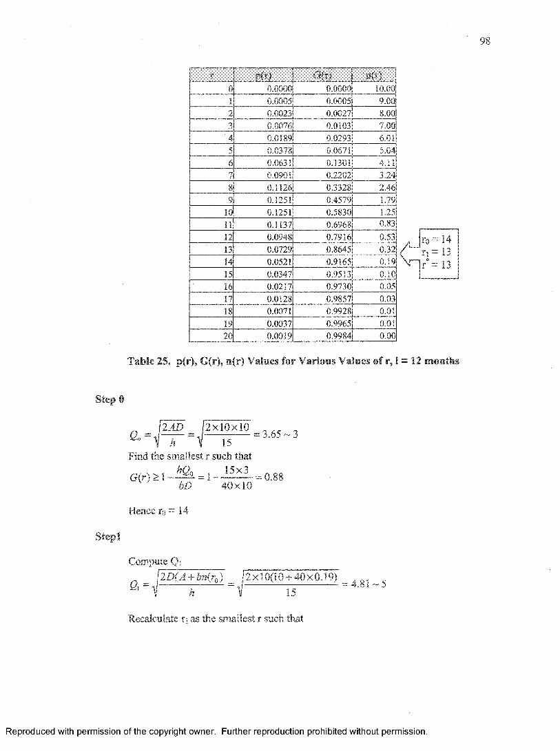
98
m ) ..... ... l i l r ) .. l i W . .0 0.0000 0.0000 10.001 0.0005 0.0005 9.002 0.0023 0.0027 8.003 0.0076 0.0103 7.004 0.0189 0.0293 6.015 0.0378 0.0671 5.046 0.0631 0.1301 4.117 0.0901 0.2202 3.248 0.1126 0.3328 2.469 0.1251 0.4579 1.79
10 0.1251 0.5830 1.2511 0.1137 0.6968 6.8312 0.0948 0.7916 0.5313 0.0729 0.8645 0.3214 0.0521 0.9165 0.1915 0.0347 0.9513 0.1016 0.0217 0.9730 0.0517 0.0128 0.9857 0.0318 0.0071 0.9928 0.0119 0.0037 0.9965 0.0120 0.0019 0.9984 0.00
Table 25. p(r), G(r), it(r) Values for Various Values of r, 1 = 12 months
Step §
2AD 2x10x10 „ „ „a=b r =\Hj- =3'65~3Find the smallest r such that
G(r) > 1 - - ^ - = I - - 1-— --- = 0.88 bD 40x10
Hence ro = 14
Stepl
Compute QiQ = 12D(A + bn(r0) 12x10(10 + 40x0.19) , f
1 h 1 15
Recalculate \\ as the smallest r such that
Reproduced with permission of the copyright owner. Further reproduction prohibited without permission.
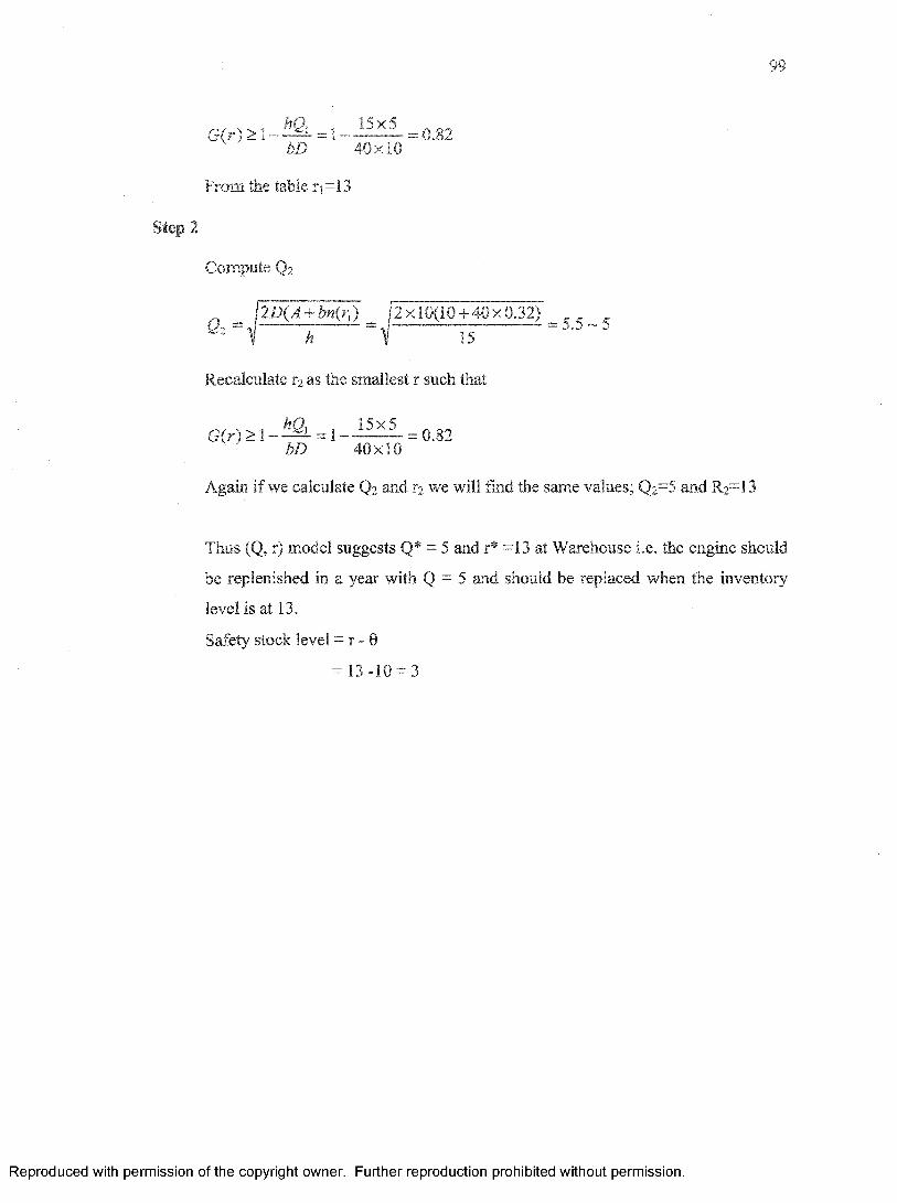
99
From the table ri=13
Step 2
Compute Q2
j2D(A + bn(rl) _ |2 x 10(10+ 40x0.32)i = 5 .5 -5h 15
Recalculate r2 as the smallest r such that
Again if we calculate Q2 and r2 we will find the same values; Q2=5 and R2=13
Thus (Q, r) model suggests Q* = 5 and r* =13 at Warehouse i.e. the engine should
be replenished in a year with Q = 5 and should be replaced when the inventory
level is at 13.
Safety stock level = r - 0
= 13-10 = 3
Reproduced with permission of the copyright owner. Further reproduction prohibited without permission.

100
Location - Primary Supplier.
t }>(r) c v ; n o n ;0 0.00 0.00 13.001 0.00 0.00 12.002 0.00 0.00 11.003 0.00 0.00 10.004 0.00 0.00 9.005 0.01 0.01 8.016 0.02 0.03 7.027 0.03 0.05 6.048 0.05 0.10 5.109 0.07 0.17 4.2010 0.09 0.25 3.3611 0.10 0.35 2.6112 0.11 0.46 1.9713 0.11 0.57 1.4314 0.10 0.68 1.00
15 0.09 0.76 0.6816 0.07 0.84 0.4417 0.05 0.89 0.2818 0.04 0.93 0.1719 0.03 0.96 0.10
A lr° = 16/ X] = 16
r =16
Table 26. p(r), G(r), n(r) Values for Various Values of r, I = 12 months
Step 02 AD 2.10.13
= 4 . 1 6 - 4
Find the smallest r such that
G(r) > 1 - ^ = 1 - = 0.83bD 40.13
Stepl
Hence r© = 16
Compute Qj
Q\ ~ 11j2D(A + bn(r0) _ j2x13(10 + 40x0.44)
h 15= 6 . 9 - 7
Reproduced with permission of the copyright owner. Further reproduction prohibited without permission.

101
Recalculate rj as the smallest r such that
G(r) > 1 - - ^ = 1 - - - - - - - = 0.82bD 40x13
From the table ri—16
Again if we calculate Q2 and r?_ wTe will find the same values; Q2 = 7 and 12 = 16
Thus (Q, r) model suggests Q*=7 and r* =16 at Primary Supplier i.e. the engine
should be replenished in a year with Q* = 7 and should be replaced when the
inventory level is at 16.
Safety stock is 16-13 = 3
Reproduced with permission of the copyright owner. Further reproduction prohibited without permission.
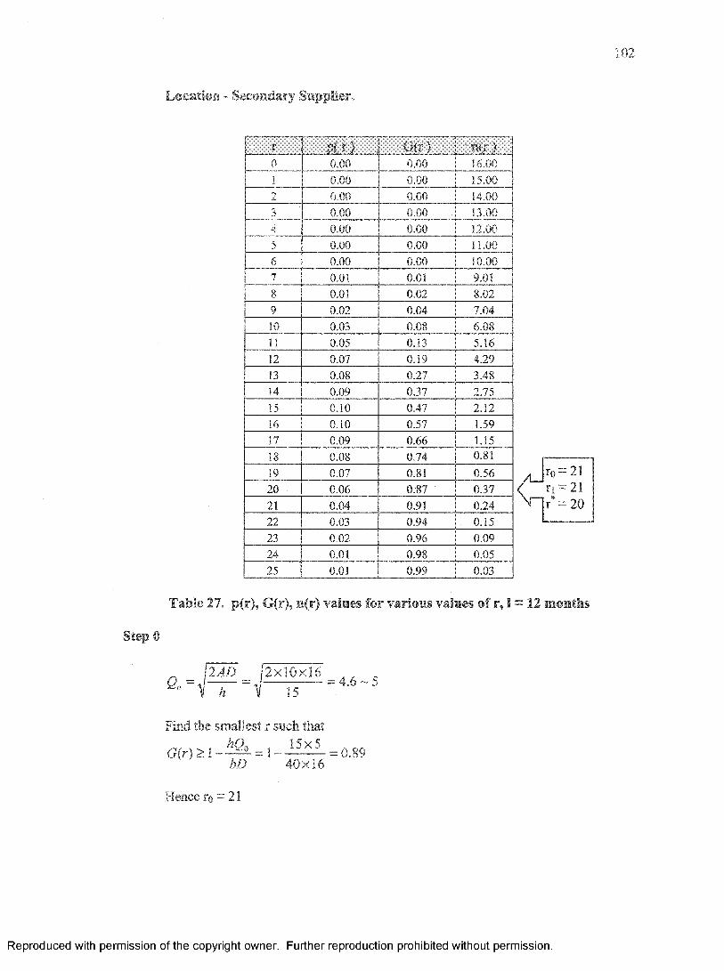
102
Location - Secondary Supplier.
1 pi r ) I k r ! ; it(r | ''0 0.00 0.00 16.001 0.00 0.00 15.002 0.00 0.00 14.00nJ 0.00 0.00 13.004 0.00 0.00 12.005 0.00 0.00 11.006 0.00 0.00 10.007 0.01 0.01 9.018 0.01 0.02 8.029 0.02 0.04 7.0410 0.03 0.08 6.0811 0.05 0.13 5.1612 0.07 0.19 4.2913 0.08 0.27 3.4814 0.09 0.37 2.7515 0.10 0.47 2.1216 0.10 0.57 1.5917 0.09 0.66 1.1518 0.08 0.74 0.8119 0.07 0.81 0.5620 0.06 0.87 0.3721 0.04 0.91 0.2422 0.03 0.94 0.1523 0.02 0.96 0.0924 0.01 0.98 0.0525 0.01 0.99 0.03
/ i_ i r» = 2 1< r, = 21
- 20
Table 27. p(r), G(r), n(r) values for various values of r, 1 = 12 months
Step 0
& = J 2 AD= J 2 x l 0 x l 6 ^ 6 _ s15
Find the smallest r such that
<JW> 1_ t a = , _ i ^ i = 0 .89bD 40x16
Hence r<> = 21
Reproduced with permission of the copyright owner. Further reproduction prohibited without permission.

103
S tep l
Compute Qjl2D(A + bn(r0) 12x16(10 + 40x0.24) . _q — ---------------- — = i— — — ------—-----— = 6.46 ~ 7
^ V h 1 15
Recalculate ij as the smallest r such that
G(r) > 1- ^ - = 1 - 13X7 = 0.84 bD 40x16
From the table i\ - 20
Step 2
= 2D(A + bn(n ) = 2x16(10 + 40x0.37) ? 2?V h V 15
Recalculate X\ as the smallest r such that
G(r) > 1 - = 1 - 1 5 X 7 = 0.84 bD 40x16
From the table X2 — 20
Again if we calculate Q3 and r3 we will find the same values; Q3 = 7 and 13 = 20
Thus (Q, r) model suggests Q* —1 and r* =20 at warehouse i.e. the engine should
be replenished in a year with Q* =7 and should be replaced when the inventory
level reaches 20.
Safety stock is 20 -16 = 4
Reproduced with permission of the copyright owner. Further reproduction prohibited without permission.

104
7.2 Replenishment Lead time Is 8 months
Warehouse (Engine)
r = 9 0 = 5
Customer (Engine)
Demand =10 units /year
PrimarySupplier (Engine)
r= 12Q = 6
Secondary Supplier
(engine parts) r= 16 0 = 7
Location - Warehouse
Annual demand is D = 10 units/year
Unit cost of the part = $150
Annual holding cost h = $15
Average demand during a replenishment lead time is
7) , 1 0 „ . „ .0 x / = — x 8 = 6.67 units
12 months 12
The cost of stockout = b = $40
Let us model the demand using Poisson distribution.
We model the demand based upon Poisson distribution:
0 re~6p(r) = Probability {Demand during lead time = r} = -------
rlr
And G (r) Cumulative Probability Distribution = p(k)k =0
Number of backorders in a replenishment cycle, n(r) = 0 p(r ) + (0 - r ) ( l - G ( r »
W e -10
rl
___ ^ 1 0 * e -10
~ L Mk=0
Reproduced with permission of the copyright owner. Further reproduction prohibited without permission.
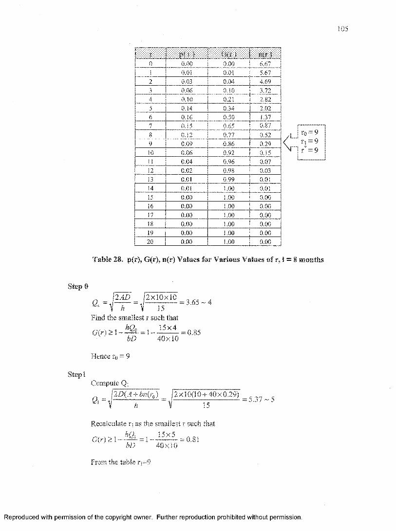
105
i......7 ....0
p{ r } 0 .0 0 0 .0 0
....m j6.67
1i 0.01 0.01 5.672 0.03 0.04 4.693 0.06 0 .1 0 3.724 0 .1 0 0.21 2.825 0.14 0.34 2.026 0.16 0.50 1.377 0.15 0.65 0.878 0.12 0.77 0.529 0.09 0.86 0.2910 0.06 0.92 0.1511 0.04 0.96 0.0712 0.02 0.98 0.0313 0.01 0.99 0.0114 0.01 1.00 0.0115 0.00 1.00 0.0016 0.00 1.00 0.0017 0.00 1.00 0.0018 0.00 1.00 0.0019 0.00 1.00 0.0020 0.00 1.00 0.00
Table 28. p(r), G(r), n(r) Values for Various Values of r, 1 = 8 months
Step 0
ft J M ? ?*»»<«> = 3 . 6 5 - 40 1 h 1 15
Find the smallest r such thatG( r ) > i _ t a = l _ i 5 ^ i = a 8 5
bD 40x10
Hence ro = 9
SteplCompute Qi^ \2D(A + bn(r0) ]2x!0(10 + 40x0.29) c cQi = -------- = J ------------ = '5-3 / - 5
Recalculate r i as the smallest r such that
G(r) > 1 - M . = = 0.81hD 40x10
From the table ij=9
Reproduced with permission of the copyright owner. Further reproduction prohibited without permission.

106
Again if we calculate Q?. and i2 we will find the same values; Q2=5 and R.2=9
Thus, (Q, r) model suggests Q* = 5 and r* = 9 at Warehouse i.e. the engine should
be replenished in a year with Q* = 5 and should be replaced when the inventory
level is at 9.
Safety stock level w r- 0 = 9-6.67 = 2.33
Location - Prim ary Supplier.
r0= 13n = i2 r*= 12
Table 29. p(r), G(r), n(r) Values for Various Values of r, 1 = 8 months
r W.r) O il) n ( r )0 0.00 0.00 9.00i 0.00 0.00 8.002 0.00 0.01 7.003 0.01 0.02 6.014 0.03 0.05 5.035 0.06 0.12 4.086 0.09 0.21 3.207 0.12 0.32 2.418 0.13 0.46 3.739 0.13 0.59 1.19
10 0.12 0.71 0.7711 0.10 0.80 0.4812 0.07 0 .8 8 0.2813 0.05 0.93 0.1614 0.03 0.96 0.0815 0.02 0.98 0.0436 0.01 0.99 0.0217 0.01 0.99 0.0118 0.00 1.00 0.0019 0.00 1.00 0.0020 0.00 1.00 0.00
Step 02 AD 2x10x13.5 „
q = |—-— = ------- ------= 4.24 ~ 4\ h V 15
Find the smallest r such thatHO 1 5 v 4
G(r) > 1 - - ^ 2 - = 1 ---- — ------= 0.89; hencerP = 13bD 40x13.5
Reproduced with permission of the copyright owner. Further reproduction prohibited without permission.
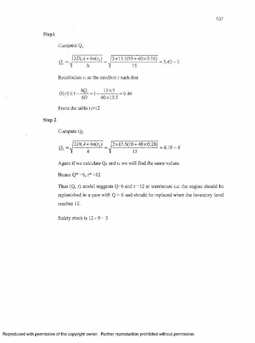
107
Stepl
Compute Qi
^ j2D(A + bn(r0) 12x13.5(10 + 40x0.16) ch " V 15 5.4j
Recalculate ip as the smallest r such that
G(, ) a l _ * a = 1 _ _ L ? i 5 _ = o.86bD 40x13.5
From the table ij=12
Step 2
Compute Q2
l2D(A + bn(r0) 12x13.5(10 + 40x0.28)= 6 . 1 8 -6
15
Again if we calculate Q3 and r3 we will find the same values.
Hence Q* =6, r* =12
Thus (Q, r) model suggests Q=6 and r =12 at warehouse i.e. the engine should be
replenished in a year with Q = 6 and should be replaced when the inventory level
reaches 12.
Safety stock is 12 -9 = 3
Reproduced with permission of the copyright owner. Further reproduction prohibited without permission.

108
73 Replenishment Lead time = 6 months
Customer (Engine)
Demand = 10 units /year
Warehouse(Engine)
Q = 4
PrimarySupplier (Engine)
r = 10
Secondary Supplier
(engine parts) r = 14 0 = 7
Location - Warehouse
Annual demand is D = 10 units/year
Unit cost of the part = $150
Annual holding cost h = $15
Average demand during a replenishment lead time is
D , 10 . c .q - ------------x / = — x 6 = 5 units12 months 12
The cost of stockout = b = $40
Let us model the demand using Poisson distribution.
We model the demand based upon Poisson distribution:
p(r) = Probability (Demand during lead time = r}: 6 re e W e - 1 0
rl rlr r
And G (r) Cumulative Probability Distribution = p(k) = A 10Ae_1°
k - 0 k =0 k\
Number of backorders in a replenishment cycle, n(r) = 0 p(r) +
Reproduced with permission of the copyright owner. Further reproduction prohibited without permission.
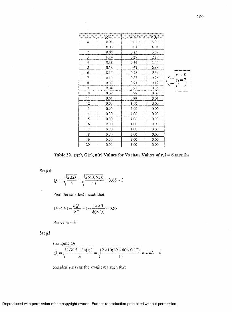
109
0.180.15
i.040.020.010.001.00
0.000.000.000.000.000.000.00
Table 30. p(r), G(r), n(r) Values for Various Values of r, 1 = 6 months
Step 02JD 2X20X10
1 i V 15
Find the smallest r such that
G ( r ) > l _ h Q l. = l _ = 0.88bD 40x10
Hence r0 = 8
Stepl
Compute Qi^ \2D(A + bn(r0) |2xl0(10 + 40x0.12) „ „Q i~ i h 1 15 - 4 .4 4 - 4
Recalculate r; as the smallest r such that
Reproduced with permission of the copyright owner. Further reproduction prohibited without permission.

From the table t\ = 1
itei
0 . = aIl2D(A + bn(rJ _ j 2x10(10 + 40x0.12) I h 15
= 5.21 ~ 5
= 0.8240x10
From the table r2 = 7
Again if we calculate Q2 and r2 we will find the same values, Q2 = 4 and r2 = 7.
Hence, (Q, r) model suggests Q* = 4 and r* = 7 at warehouse, the engine should
be replenished in a year with Q* = 4 and should be replaced when the inventory
level reaches 7.
Safety stock level = r - 0
Location - Prim ary Supplier.
Primary supplier has to supply 7 items for 6 months and hence the demand for year is 14
items per year.
Total demand is 14 and the average demand is 7.
7 - 5 = 2
Reproduced with permission of the copyright owner. Further reproduction prohibited without permission.

I l l
0 0.00<ifr)0.00
n i p )7.00
1 0.01 0.01 6.002 0.02 0.03 5.013 0.05 0.08 4.044 0.09 0.17 3.125 0.13 0.30 2.296 0.15 0.45 1.597 0.15 0.60 1.048 0.13 0.73 0.649 0.10 0.83 0.3710 0.07 0.90 0.2011 0.05 0.95 0.1012 0.03 0.97 0.0513 0.01 0.99 0.0214 0.01 0.99 0.0115 0.00 1.00 0.0016 0.00 1.00 0.0017 0.00 1.00 0.0018 0.00 1.00 0.0019 0.00 1.00 0.0020 0.00 1.00 0.00
r0 =10n = 10 r = 10
Table 31. p(r), G(r), n(r) Values for Various Values of r, 1 = 6 months
Step 0
2 AD 2.10.14\ h V 15
= 4 . 3 2 - 4
Find the smallest r such that
G(r) > 1 - = 1 - — — = 0.89
Stepl
bD
Hence r0 = 10
Compute Qi
a
40x14
2D(A + bn(r0) *2x14(10 + 40x0.20)15
= 5 . 7 9 - 6
Recalculate rj as the smallest r such that
Reproduced with permission of the copyright owner. Further reproduction prohibited without permission.

112
G(r) > = 1----- — - = 0.84bD 40x14
From the table rj=10
Again if we calculate Q2 and we will find the same values.
Hence Q* = 6, f* =10
Thus, (Q, r) model suggests Q* = 6 and r* = 10 at primary supplier i.e. the engine
should be replenished in a year with Q* = 6 and should be replaced when the
inventory level reaches 10.
Safety stock is 10-7 = 3
Location - Secondary Supplier.
r A . ' W ) ' 7 v 1 # . .0 0.00 0.00 10.001 0.00 0.00 9.002 0.00 0.00 8.003 0.01 0.01 7.004 0.02 0.03 6.015 0.04 0.07 5.046 0.06 0.13 4.117 0.09 0.22 3.248 0.11 0.33 2.469 0.13 0.46 1.7910 0.13 0.58 1.2511 0.11 0.70 0.8312 0.09 0.79 0.53
13 0.07 0.86 0.3214 0.05 0.92 0.1915 0.03 0.95 0.1016 0.02 0.97 0.0517 0.01 0.99 0.0321 0.00 1.00 0.0022 0.00 1.00 0.0023 0.00 1.00 0.00
\r rr0= 14 n = 14
= 14
Table 32. p(r), G(r), n(r) Values for Various Values of r, 1 = 6 months
Reproduced with permission of the copyright owner. Further reproduction prohibited without permission.

113
Step 0
a = J ^ £ = ,&S1252® =5.16-5\< A II 15
Find the smallest r such that
G W > , _ i a = 1 _ J t £ i = o.9ibD 40x20
Hence ro = 14
Stepl
Compute Qi
a =2D(A + bn(r0) _ 2x20(10 + 40x0.19) _
— 6.85 ~ 71 h V 15
Recalculate ri as the smallest r such that
G(r) > 1 - ^ L = 1 - 15X7 = 0.87 bD 40x20
From the table ri=14
Step 2
After recalculating Q2 =7 and t~i - 14
Thus, (Q, r) model suggests Q* = 7 and x* = 14 at Secondary Supplier i.e. the
engine should be replenished in a year with Q* = 7 and should be replaced when
the inventory level reaches 14.
Safety stock is 14-10 = 4
Reproduced with permission of the copyright owner. Further reproduction prohibited without permission.

7,4 Replenishment Lead time = 4 months
Customer (Engine)
Demand =10 units /year
Warehouse(Engine)
Q = 5
PrimarySupplier(Engine)
Secondary Supplier
(engine parts)
0 = 8
Location Warehouse
Annual demand is D = 10 units/year
Unit cost of the part = $150
Annual holding cost fa = $15
Average demand during a replenishment lead time is
0 = -----—-----x / = — x4 = 3.33 units12 months 12
The cost of stockout = b = $40
Let us model the demand using Poisson distribution.
We model the demand based upon Poisson distribution:
0 re~e 10W 10p(r) = Probability {Demand during lead time = r} = --------= ----------
r\ r\
r , r l0 /cg~!CAnd G (r) Cumulative Probability Distribution = p(k) =
k - 0 k=0 k\
Number of backorders in a replenishment cycle, n(r) ~ 0 p(r ) + ( 0 - r)(l - Gir))
Reproduced with permission of the copyright owner. Further reproduction prohibited without permission.
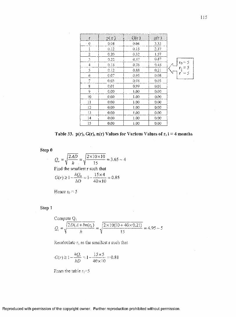
115
rt(r >
0.00
Table 33. p(r), G(r), n(r) Values for Various Values of r, 1 = 4 months
Step 0
Find the smallest r such that
G(r) > , - ^ = l - i ^ = 0.85 bD 40x10
Hence r0 = 5
Step 1
Compute Qi^ 12D(A + bn(r0) _ |2xl0(10 + 40x0.21) „ nc c
? h 1 15
Recalculate rj as the smallest r such that
G ( r ) > 1 - h^L = 1 - = 0.81bD 40x10
From the table ri=5
Reproduced with permission of the copyright owner. Further reproduction prohibited without permission.
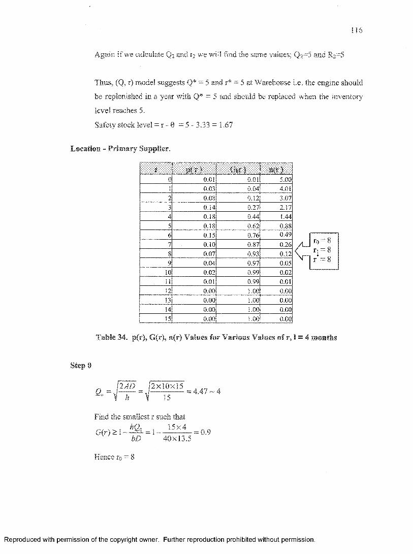
116
Again if we calculate Q2 and r2 we will find the same values; Q2=5 and R2=5
Thus, (Q, r) model suggests Q* = 5 and r* = 5 at Warehouse i.e. the engine should
be replenished in a year with Q* = 5 and should be replaced when the inventory
level reaches 5.
Safety stock level = r - 0 = 5 - 3.33 = 1.67
Location - Prim ary Supplier.
0P( 3") __
0.0?» t f )
0.01n t f )
5.001 0.03 0.04 4.012 0.08 0.12 3.073 0.14 0.27 2.174 0.18 0.44 1.445 0.18 0.62 0.886 0.15 0.76 0.497 0.10 0.87 0.268 0.07 0.93 0.129 0.04 0.97 0.05
10 0.02 0.99 0.0211 0.01 0.99 0.0112 0.00 1.00 0.0013 0.00 1.00 0.0014 0.00 1.00 0.0015 0.00 1.00 0.00
Table 34. p(r), G(r), n(r) Values for Various Values of r, 1 = 4 months
Step 0
2AD fi2 x l 0 x l 5 „ ^ ,Go = J = J — = 4.47 ~ 4
\ h \ 15
Find the smallest r such that
G ( r ) > 1 - ^ = 1 ----- = 0.9bD 40x13.5
Hence ro = 8
Reproduced with permission of the copyright owner. Further reproduction prohibited without permission.

117
Stepl
Compute Qi
^ j2D(A + bn(r0) f2xl3.5(ldT40^0A2) c 4/1 ch 15 44 ~5
Recalculate t\ as the smallest r such that
G(r) > = =bD 40x15
From the table ri=8
Step 2
Again if we calculate Q2 and r2 we will find the same values.
Hence Q* =5, r* =8
Thus (Q, r) model suggests Q* = 5 and r* = 8 at Primary Supplier i.e. the engine
should be replenished in a year with Q* = 5 and should be replaced when the
inventory level reaches 8.
Safety stock is 8 -5 =3
Reproduced with permission of the copyright owner. Further reproduction prohibited without permission.
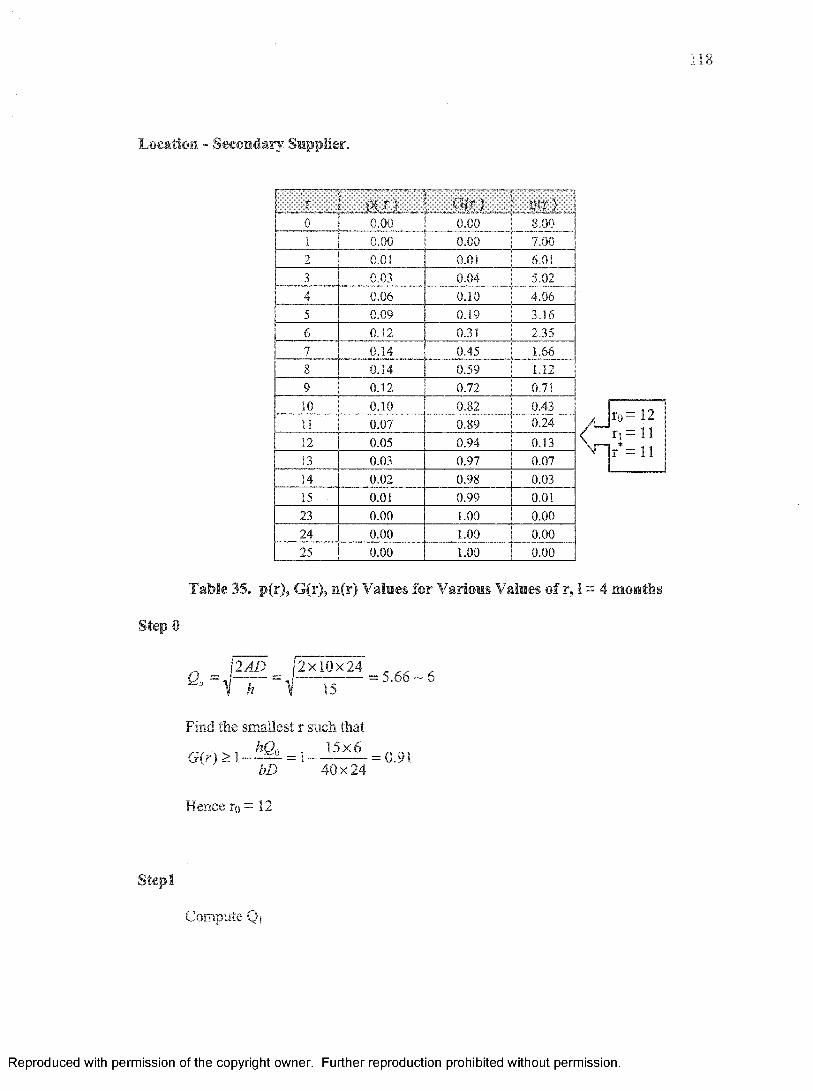
Location - Secondary Supplier.
0 0.00 0.00 8.001 0.00 0.00 7.002 0.01 0.01 6.013 0.03 0.04 5.024 0.06 0.10 4.065 0.09 0.19 3.166 0.12 0.31 2.357 0.14 0.45 1..668 0.14 0.59 1.129 0.12 0.72 0.7110 0.10 0.82 0.431! 0.07 0.89 0.24
12 0.05 0.94 0.1313 0.03 0.97 0.0714 0.02 0.98 0.0315 0.01 0.99 0.0123 0.00 1.00 0.0024 0.00 1.00 0.0025 0.00 1.00 0.00
r0- 12rj[ — 11 r* = 11
Table 35. p(r), G(r), n(r) Values for Various Values of r, 1 = 4 months
Step 0
2AD 2 X 1 0 X 2 4
° V h V 15
Find the smallest r such that
G(r) > \ - ^ L = 1- 15x6 = 0.91bD 40x24
Hence ro = 12
Stepl
Compute Qi
Reproduced with permission of the copyright owner. Further reproduction prohibited without permission.
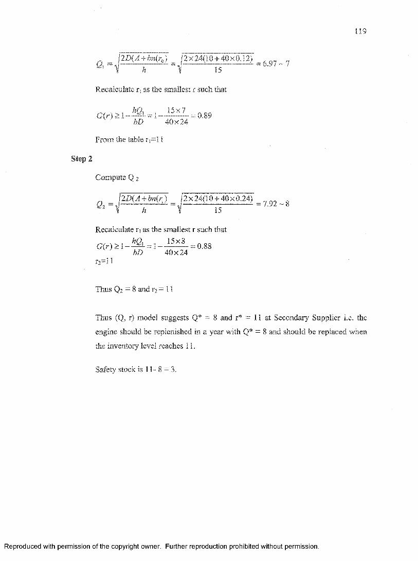
119
^ [2D(A + bn(r0) |2 x 24(10 + 40x012) ^ n„ „(j — — = j --------- —______ = 5_y / ~ /^ V A V 15
Recalculate ri as the smallest r such that
G(r) > 1 - = 1 - J l l L = o,89 bD 40x24
From the table r j= l!
Step 2
Compute Q 2
= \2D(A + bn(rx) 12x24(10 + 40x024) gi h V 15
Recalculate rj as the smallest r such that
G(r) > 1 - ^ = 1 - = 0.88 bD 40x24
r2= l l
Thus Q2 = 8 and r2 = 11
Thus (Q, r) model suggests Q* = 8 and r* = 11 at Secondary Supplier i.e. the
engine should be replenished in a year with Q* = 8 and should be replaced when
the inventory level reaches 11.
Safety stock is 11- 8 = 3.
Reproduced with permission of the copyright owner. Further reproduction prohibited without permission.

120
7.5 Replenishment lead time = 2 months
Warehouse (Engine)
r = 3Q = 4
Customer(Engine)
Demand =10 units /year
PrimarySupplier(Engine)
r = 5 Q - 6
SecondarySupplier
(engine parts)
Location - Warehouse
Annual demand is D = 10 units/year
Unit cost of the part = $150
Annual holding cost h = $15
Average demand during a replenishment lead time is
D , 1 0 „ , „ .0 = ------------- x / = — x2 = 1.67 units12 months 12
The cost of stockout = b = $40
Let us model the demand using Poisson distribution.
We model the demand based upon Poisson distribution:
0 re~d \0re~mp(r) = Probability (Demand during lead time = r} = --------= ----------
r\ r\
r r j(p g ~10And G (r) Cumulative Probability Distribution = p(k) =---- ----------
i=0 ?c=0
Number of backorders in a replenishment cycle, n(r) = 9 p{r) +
Reproduced with permission of the copyright owner. Further reproduction prohibited without permission.
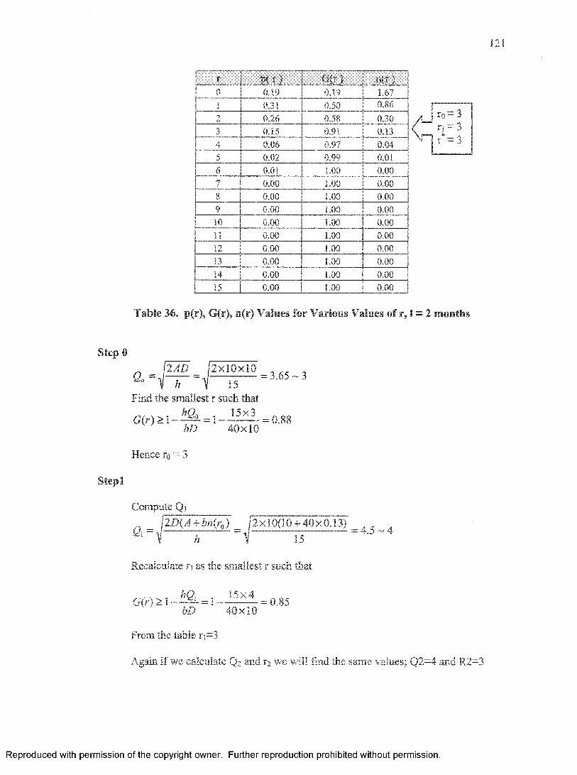
■' r fHrt ) ;i ' ■■ " n ( f > -0 0.19 0.19 1.671 0.31 0.50 0.862 0.26 0.58 0.303 0.15 0.91 0.134 0.06 0.97 0.045 0.02 0.99 0.016 0.01 1.00 0.007 0.00 1.00 0.008 0.00 1.00 0.009 0.00 1.00 0.0010 0.00 1.00 0.0011 0.00 1.00 0.0012 0.00 1.00 0.0013 0.00 1.00 0.0014 0.00 1.00 0.0015 0.00 1.00 0.00
Table 36. p(r), G(r), n(r) Values for Various Values of r, 1 = 2 months
Step 0
Find the smallest r such that
G ( r ) > l - ^ = 1 - 15X3 =0.88 bD 40x10
Hence % = 3
Stepl
Compute Qij2D(A + bn(r0) = /2xl0(10 + 40x0.13) = 4 5 4
1 1 h 15
Recalculate ij as the smallest r such that
G(r) > 1 = 1 — = o.85M) 40x10
From the table ri—3
Again if we calculate Q2 and 12 we will find the same values; Q2=4 and R2=3
Reproduced with permission of the copyright owner. Further reproduction prohibited without permission.

122
Thus (Q, r) mode! suggests Q* = 4 and r* = 3 at Warehouse i.e. the engine should
be replenished in a year with Q* = 4 and should be replaced when the inventory
level reaches 3.
Safety stock level = r - 0
= 3 -1.67 = 1.33
Location - Primary Supplier.
■ Pt r ). G(r) n i t )
0 0.05 0.05 3.001 0.15 0.20 2.052 0.22 0.37 1.303 0.22 0.65 0.674 0.17 0.82 0.325 0.10 0.92 0.136 0.05 0.97 0.057 0.02 0.99 0.028 0.01 1.00 0.019 0.00 1.00 0.0010 0.00 1.00 0.0011 0.00 1.00 0.0012 0.00 1.00 0.0013 0.00 1.00 0.0014 0.00 1.00 0.0015 0.00 1.00 0.00
< w : =V i r*=
r0=5 5 5
Table 37. p(r), G(r), n(r) Values for Various Values of r, 1 = 2 months
Step #
Qo =2 AD 2x10x18
V h 15= 4 . 9 - 5
Find the smallest r such that
G{r) > 1- ^ . = i = o,90bD 40x18
Hence ro = 5
Step!
Compute Qi
Reproduced with permission of the copyright owner. Further reproduction prohibited without permission.

123
n = ! E ^ ± t M y = f2xT8(i0 + 40xb.l3)' 1 h 1 15
Recalculate rt as the smallest r such that
G(r ) > j - = i _ ...L I * ! = 0 . 8 8M) 40x18
From the table ri=5
Again if we calculate Cb and 12 we will find the same values.
Hence Q* =6, r* =5
Thus (Q, r) model suggests Q* = 6 and r* = 5 at Primary Supplier i.e. the engine
should be replenished in a year with Q* = 6 and should be replaced when the
inventory level reaches 5.
Safety stock is 5 - 3 = 2
Reproduced with permission of the copyright owner. Further reproduction prohibited without permission.
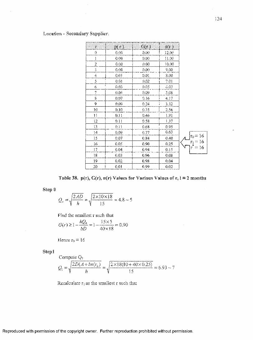
124
Location - Secondary Supplier.
......." ............. -V- V... t »(r ) n(T )0 0.00 0.00 12.001 0.00 0.00 11.002 0.00 0.00 10.003 0.00 0.00 9.004 0.01 0.01 8.005 0.01 0.02 7.016 0.03 0.05 6.037 0.04 0.09 5.088 0.07 0.16 4.179 0.09 0.24 3.3210 0.10 0.35 2.5611 0.11 0.46 1.9112 0.11 0.58 1.3713 0.11 0.68 0.9514 0.09 0.77 0.6315 0.07 0.84 0.4016 0.05 0.90 0.2517 0.04 0.94 0.1518 0.03 0.96 0.0819 0.02 0.98 0.0420 0.01 0.99 0.02
r0 = 16n = i 6 r*= 16
Table 38, p(r), G(r), n(r) Values for Various Values of r, 1 = 2 months
Step #& = J 2 d £ = J 2 x l 0 x l S =Jks_ s
h 15
Find the smallest r such that
G(r) > 1 •bD
15x540x18
= 0.90
Hence r0 = 16
SteplCompute Qi
f i =2D(A + bn(rQ) _ j 2 x 18(10 + 40 x 0.25)
h 15= 6.93 ~ 7
Recalculate rj as the smallest r such that
Reproduced with permission of the copyright owner. Further reproduction prohibited without permission.
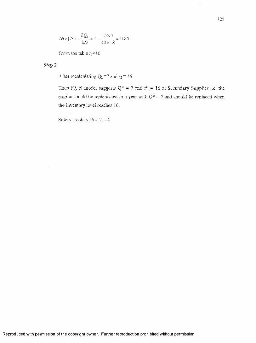
125
G(r) > 1 = 1 - 15X7 = 0.85bD 40x18
From the table ri=16
Step 2
After recalculating Q? ~1 and r? = 16
Thus (Q, r) model suggests Q* - 7 and r* = 16 at Secondary Supplier i.e. the
engine should be replenished in a year with Q* = 7 and should be replaced when
the inventory level reaches 16.
Safety stock is 16 -12 = 4
Reproduced with permission of the copyright owner. Further reproduction prohibited without permission.
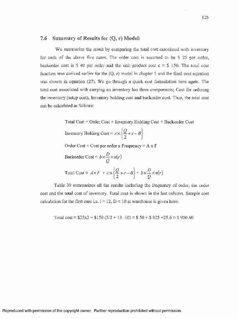
126
7.6 Summary of Results for (Q, r) Model:
We summarize the result by comparing the total cost associated with inventory
for each o f the above five cases. The order cost is assumed to be S 25 per order,
backorder cost is $ 40 per order and the unit product cost c = $ 150. The total cost
function was derived earlier for the (Q, r) mode! in chapter 5 and the final cost equation
was shown in equation (21). We go through a quick cost formulation here again. The
total cost associated with carrying an inventory has three components; Cost for ordering
the inventory (setup cost), Inventory holding cost and backorder cost. Thus, the total cost
can be calculated as follows:
Total Cost = Order Cost + Inventory Holding Cost + Backorder Cost
Inventory Holding Cost = cx j-^ + r - $ j
Order Cost = Cost per order x Frequency = A x F
Backorder Cost — b x — x nir)Q
Total Cost = A x F + c x \ - + r - 0 1+ b x — xn(r)12 J 0
Table 39 summarizes all the results including the frequency of order, the order
cost and the total cost of inventory. Total cost is shown In the last column. Sample cost
calculation for the first case i.e. 1 = 12, D = 10 at warehouse is given here:
Total cost = $25x2 + $150 (5/2 + 13 -10) = $ 50 + $ 825 +25.6 = $ 900.60
Reproduced with permission of the copyright owner. Further reproduction prohibited without permission.

s mi-
***'hi
. nr1 b
M ^ ; . | o f
ft
' IIs I Ii ■ f t
1 1 SB w
*§ <* I f ' ..y
ij'.**
■■O !Q1 :
12 WH 0.32 13.00 5.00 0.94 2.00 10 825 25.6 50.00 900.60PS 0.44 16.00 7.00 0.94 1.86 13 975 32.7 46.43 1054.10ss 0.37 20.00 7.00 0.95 2.29 16 1125 33.8 57.14 1216.00
6 WH 0.26 7.00 4.00 0.94 2.50 5 600 26 62.50 688.50PS 0.20 10.00 6.00 0.97 2.33 / 900 18.7 58.33 977.00ss 0.19 14.00 7.00 0.97 2.86 10 1125 21.7 71.43 1218.10
2 WH 0.13 3.00 4.00 0.97 2.50 1.67 499.5 13 62.50 575.00PS 0.13 5.00 6.00 0.98 3.00 3 750 15.6 75.00 840.60ss 0.12 8.00 8.00 0.99 3.75 5 1050 18 93.75 1161.80
8 WH 0.29 9.00 5.00 0.94 2.00 6.67 724.5 23.2 50.00 797.70PS 0.28 12.00 6.00 0.95 2.25 9 900 25.2 56.25 981.50SS 0.25 16.00 7.00 0.96 2.57 12 1125 25.7 64.29 1215.00
4 w e 0.21 5.00 5.00 0.96 2.00 3.33 625.5 16.8 50.00 692.30PS 0.12 8.00 5.00 0.98 3.00 5 825 14.4 75.00 914.40SS 0.24 11.00 8.00 0.97 3.00 8 1050 28.8 75.00 1153.80
Table 39. Summary of Application Runs for (Q, r) Model
■ ’ f c l i l T I»e ■ ;■ . f tiw ilta l CrniM
frl*aswf Snjpiplfcr. S fcon ia ry ' ’ Storage Cmt <11,
12 900.60 1054.10 1216.008 797.70 981.50 1215.006 688.50 977.00 1218.104 692.30 914.40 1153.802 575.00 840.60 1161.80
Reproduced with permission of the copyright owner. Further reproduction prohibited without permission.
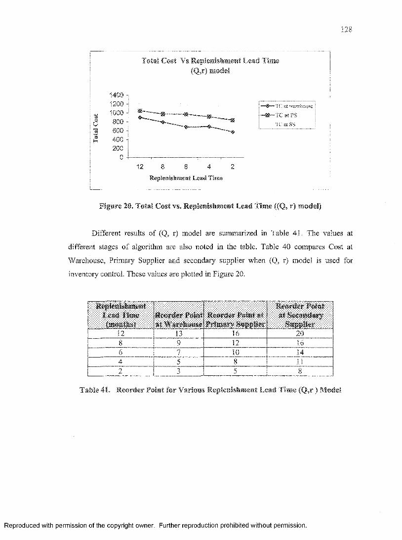
128
Total Cost Vs Replenishment Lead Time (Q,r) model
o
2aH
140012001000800600400200
012 8 6 4 2
Replenishment Lead Time
at warehouse
"HBf™TC at PS TC at SS
Figure 20. Total Cost vs. Replenishment Lead Time ((Q, r) model)
Different results of (Q, r) model are summarized in Table 41. The values at
different stages of algorithm are also noted in the table. Table 40 compares Cost at
Warehouse, Primary Supplier and secondary supplier when (Q, r) model is used for
inventory control. These values are plotted in Figure 20.
Replenishment Lead Time(months?
Reorder Point at. Warehouse
Reorder Point atPrimary Supplier
Reorder Point at Secondary
Supplier12 13 r " 1- 1 6 208 9 12 166 7 10 144 5 8 112 3 5 8
Table 41. Reorder Point for Various Replenishment Lead Time (Q ,r) Model
Reproduced with permission of the copyright owner. Further reproduction prohibited without permission.
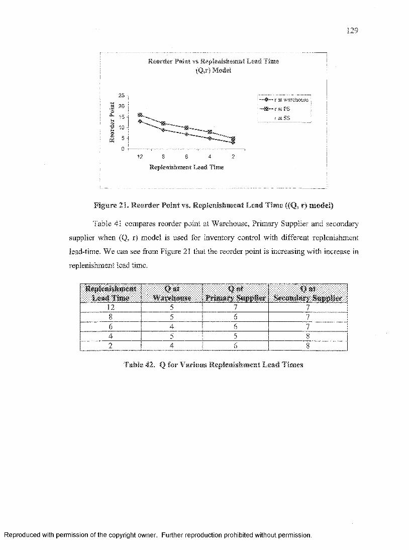
129
R eorder Point vs Replenishemnt Lead Time (Q,r) Model
25 -
20
15
10
5
06 4 212 8
Replenishment Lead Time
r at warehouserat PSratSS
Figure 21. Reorder Point vs. Replenishment Lead Time ((Q, r) model)
Table 41 compares reorder point at Warehouse, Primary Supplier and secondary
supplier when (Q, r) model is used for inventory control with different replenishment
lead-time. We can see from Figure 21 that the reorder point is increasing with increase in
replenishment lead time.
Replenishment Lead Time
Q afWarehouse
Q atPrimary Supplier
Q atSecondary Supplier
12 5 7 78 5 6 76 4 6 74 5 5 82 4 6 8
Table 42. Q for Various Replenishment Lead Times
Reproduced with permission of the copyright owner. Further reproduction prohibited without permission.

130
Chapter - 8
PHYSICAL SIMULATION OF BASE STOCK MODEL
8.1 Goals of Physical Simulation
Primary goal of conducting the physical simulation is to validate the results
obtained from the mathematical models. Simulation was ran to confirm that optimum
inventory levels i.e. reorder point at warehouse, primary supplier and secondary supplier
are realistic values. Physical simulations are being used very effectively as a teaching tool
for Lean training. Physical simulations can quickly and effectively demonstrate the effect
of organizational and process change to participants. These simulations can be used to
model stochastic systems like organizational supply chains.
8.2 Simulation Activity for Base Stock Model
This physical simulation models a three-tier single-product supply chain. ABC
company uses a certain type of engine for their product. Final assembly department of the
company withdraws these engines from the warehouse as needed. The Warehouse
receives engines from Prim ary Suppler. Prim ary Supplier receives the engine parts
like cylinders from Secondary Supplier. We will make the assumption that only one
cylinder is needed per engine. We are interested in inventory levels at Warehouse,
Prim ary Supplier and Secondary Supplier. Excessive inventory results in increased
holding costs while inadequate inventory results in backorders. Thus it is necessary to
keep the optimum level of inventory at Warehouse, Primary Supplier and Secondary
Supplier.
8.3 Simulation Layout
Customer, Warehouse, Prim ary Supplier and Secondary Supplier are 4
departments in the simulation. The movement of the parts is as shown in the Figure 22
Reproduced with permission of the copyright owner. Further reproduction prohibited without permission.

131
below. The Secondary Supplier provides cylinders to Primary Supplier. The Primary
Supplier assembles the cylinders in the Engine Block and sends the Engine to the
Warehouse. Engines are pulled from warehouse based upon a demand that follows
Poisson distribution.
Total simulation time 3 years (15 minutes), Poisson distribution for demand, Replenishment lead 'time = 1 year (5 minutes)
S u p p le r(CylteierF)
T&*?
L ♦M w iySuppler(Engine ■ iBlock) “ I f
r » ?
Warehouse(Eufbtt)
r *=? Deusuuta * Com,
Figure 22. Layout of Supply Chain for Physical Simulation
8.4 Departments
a. Customer
Customer sends the Order Requirement Form to the Warehouse of company
ABC.
b. Warehouse
This department receives the Order Requirement Form from the Customer and
sends the parts to the Customer as per the schedule.
c. Primary Supplier:
Primary Supplier receives the Order Requirement Form from the Warehouse
and sends the parts to the Warehouse as per the schedule. Primary Supplier
sends the Order Requirement Form to Secondary Supplier and receives the parts
from it.
Reproduced with permission of the copyright owner. Further reproduction prohibited without permission.
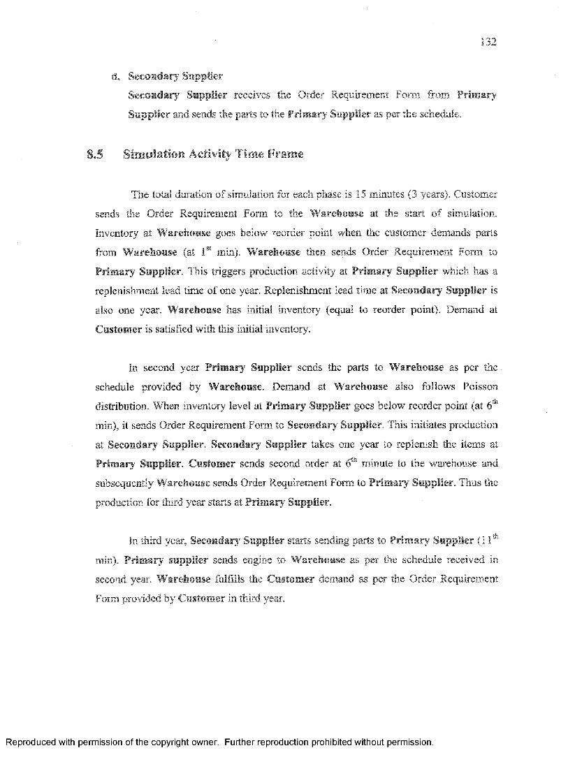
132
d. Secondary Supplier
Secondary Supplier receives the Order Requirement Form from Prim ary
Supplier and sends the parts to the Prim ary S uppler as per the schedule.
8.5 Simulation Activity Time Frame
The total duration of simulation for each phase is 15 minutes (3 years). Customer
sends the Order Requirement Form to the Warehouse at the start o f simulation.
Inventory at Warehouse goes below reorder point when the customer demands parts
from Warehouse (at 1st min). Warehouse then sends Order Requirement Form to
Primary Supplier. This triggers production activity at Primary Supplier which has a
replenishment lead time of one year. Replenishment lead time at Secondary Supplier is
also one year. Warehouse has initial inventory (equal to reorder point). Demand at
Customer is satisfied with this initial inventory.
In second year Primary Supplier sends the parts to Warehouse as per the
schedule provided by Warehouse. Demand at Warehouse also follows Poisson
distribution. When inventory level at Prim ary Supplier goes below reorder point (at 6th
min), it sends Order Requirement Form to Secondary Supplier. This initiates production
at Secondary Supplier. Secondary Supplier takes one year to replenish the items at
Primary Supplier. Customer sends second order at 6tn minute to the warehouse and
subsequently Warehouse sends Order Requirement Form to Prim ary Supplier. Thus the
production for third year starts at Primary Supplier.
In third year, Secondary Supplier starts sending parts to Primary Supplier (11lh
min). Primary supplier sends engine to Warehouse as per the schedule received in
second year. Warehouse fulfills the Customer demand as per the Order Requirement
Form provided by Customer in third year.
Reproduced with permission of the copyright owner. Further reproduction prohibited without permission.

133
8.6 Phase-I
During phase-1, amount of initial inventory is same as reorder point calculated but
lower than the quantities predicted by the mathematical model. The level of inventory is
10 items at Warehouse, 14 items at Prim ary Supplier and 19 items at Secondary
Suppler. Customer demand is 10 units per year. These values are intentionally kept
lower than the ideal values of inventory predicted by mathematical model.
Any demand not filled from stock is backordered. The number of backorders
during this phase is noted in the form provided at each department. Simulation activity
takes place and data is collected.
Base Stock model assumes replenishment quantity of one unit. Hence there is
Single Piece Flow in supply chain.
Inventory at the end of simulation at Warehouse, Prim ary Supplier and
Secondary Supplier is documented. The ideal values calculated by mathematical model
are Warehouse =14, Primary Supplier = 19. Secondary Supplier = 25. Total number
of backorders is documented and results are shown in spreadsheet.
Secondary Primary Warehouse CustomerSupplier r - A Supplier |------\ (Engine) (Engine)
(cylinders) L— y (Engine I------J r = 10 Demand =r =19 Block) r=!4 10
8.7 Phase-II
During pfaase-II, the inventory levels are kept at the optimum values predicted by
the mathematical model. The inventory levels are same as reorder points in this phase
also. With optimum levels of inventory, no backorders were documented in this phase
confirming the results predicted by mathematical models.
Reproduced with permission of the copyright owner. Further reproduction prohibited without permission.

134
Secondary Supplier
(cylinders) r = 25
£
PrimarySupplier {Engine
Block) r —19
Warehouse (Engine)
r= 14
Customer (Engine)
Demand = 10
8.8 Phase-Ill
During phase-III, the inventory levels are kept intentionally higher than the
optimum levels and the reorder points are as shown in the figure below. No backorders
were observed in this phase due to high inventory levels but inventory costs were high
due to large inventory level.
Secondary Primary WarehouseSupplier 1------\
Supplier I------\ (Engine)(cylinders) (Engine L - V r= 19
r =30 Block) r =25
Customer (Engine)
Demand =10
8.9 Distribution of Demand
We ensure that the demand at Warehouse, Primary Supplier and Secondary
Supplier follows Poisson distribution as in the case of mathematical models. This is
done by using Stat-Fit software to calculate demand quantities for Customer, Primary
Supplier and Secondary Supplier. Figure 23 shows the Stat-Fit screen for demand
calculation for a typical year.
Reproduced with permission of the copyright owner. Further reproduction prohibited without permission.
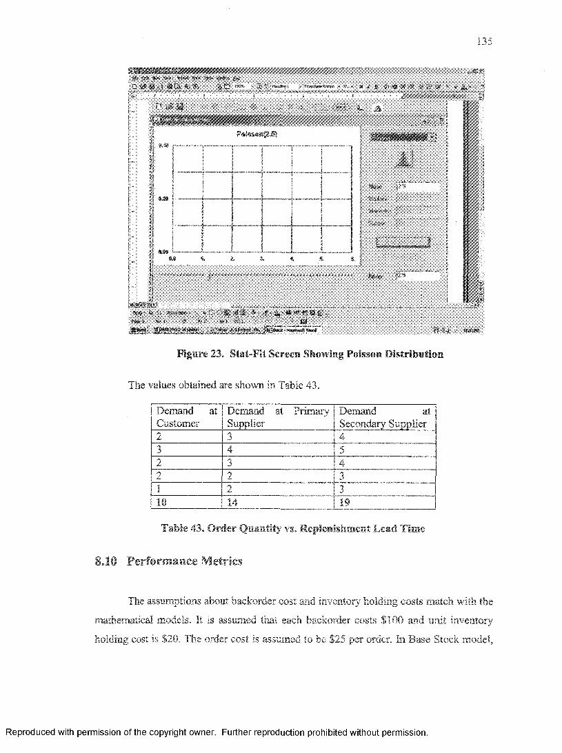
135
■ ! ^ : ; ^ # ^ :;'!:||^ S ''':':': '
C u S O d - #Gl * ■ * . 5*0 >*•= - $ •
r 2# B
V'rwjsKmRoMjn « 3?.! «.([.# f: '£:];P:|!W#:::B;|:|i;;K;S§i1:.S:: #.! ;; ■-? ’ 5' .: ..f ‘ ■ ; ' .V ■ ^^S§SS§sS S 0 B■ ■. ■ l. \ ;
ItP»is»»fip,SJ
a*
U M i
! iI ?1 s\ „ _L „ __
_ . _
1 !...... _.... ................................. .j ^
i !i . . . . 1..........! j 1! i
1 s
illilppf5MStt
„ ..................r & ' A&iS’We'i - ’ ** E ! l* J fig! S- lE ^ ' -f * & ’ ®S ~ f} Q* 4 ■.\'&te 1 '»f 1 Iff As I* to 1 Coi i &£<M«1 •*?:■•-. ■■ -' ■ • • ■ = . . ■ > . „ ,< WU..
Figure 23. Stat-Fit Screen Showing Poisson Distribution
The values obtained are shown in Table 43.
Demand at Demand at Primary Demand atCustomer Supplier Secondary Supplier2 3 43 4 52 3 42 2 31 2 310 14 19
Table 43. O rder Quantity vs. Replenishment Lead Time
8.10 Performance Metrics
The assumptions about backorder cost and inventory holding costs match with the
mathematical models. It is assumed that each backorder costs $100 and unit inventory
holding cost is $20. The order cost is assumed to be $25 per order. In Base Stock model,
Reproduced with permission of the copyright owner. Further reproduction prohibited without permission.

136
the order quantity is one therefore, total numbers of orders are same as order quantity.
Following spreadsheet is used to collect the data:
Total number of orders
1 ota! # of Back Orders Cost of each Backorder ($}
Cost of unit inventory cost Excess Inventory Cost
24 ..[33$600.00 i$825Ji
,
44illlllllB M B1 s
so p “ 0$100.00
5 ................:$10
$100.00m ............$10
$100.00r$10
$60.00 $240.00 $410.00
Table 44. Performance Metric Spreadsheet
8.11 Summary
Excess inventory and number of backorders is documented at the end of each
phase. The inventory holding cost and backorder cost are calculated in each phase. Ten
backorders were observed during phase-I because of inadequate inventory at Warehouse.
Therefore, total backorder cost is $1000 in phase-1 During phase-III, excess inventory
exists and cost associated with this inventory is $410.
Phase-II, includes the optimum level of inventory as predicted by mathematical
models. In this case, backorder cost is zero and excess inventory cost is higher than
phase-I but lower compared with phase-III. Total cost of inventory is the lowest in
Phase-II as predicted by the mathematical models. Figure 24 shows the blocks used
during simulation for engine blocks, cylinders and assembled engines. Figures 25 and 26
show the forms used during physical simulation.
Reproduced with permission of the copyright owner. Further reproduction prohibited without permission.
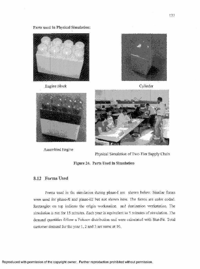
137
Parts used in Physical Simulation:
Engine Block
Assembled Engine
Cylinder
Physical Simulation of Two-Tier Supply Chain
Figure 24. Parts Used in Simulation
8.12 Forms Used
Forms used in the simulation during phase-I are shown below. Similar forms
were used for phase-II and phase-III but not shown here. The forms are color coded.
Rectangles on top indicate the origin workstation and destination workstation. The
simulation is run for 15 minutes. Each year is equivalent to 5 minutes of simulation. The
demand quantities follow a Poisson distribution and were calculated with Stat-Fit. Total
customer demand for the year 1, 2 and 3 are same at 10.
Reproduced with permission of the copyright owner. Further reproduction prohibited without permission.

138
CUSTOMER ORDER SCHEDULE
c u s t o m e r c r : “ : : r . f > w a r e h o u s e
YEAR-1
# QTYOrder Tim®
2 V.00
2 3 2:00
3 2 3:00
4 2 4:00
5 1 3:00
CUSTOMER ORDER SCHEDULE
c u s t o m e r w a r e h o u s e
YEAR-3
# QTY Order Tisw Cnb0
i 2 11:00
2 3 12:00
3 2 13:00
4 2 14:00
3 1 15:00
WAREHOUSE ORDER SCHEDULE
SOUSE IY SUPPLIERi l l
Y E A R - 1
# QTYOrder Delivery Time
(mto)
1 2 6:00
1 2 3 7:00
3 2 8:00
| 4 2 9:00
1 5 1
1 10:00
?fcese-l
PRIMARY SUPPLIER ORDER SCHEDULE
ry s u p p l i e r r~ :;T ;::r ,3 :L ;> s e c o n d a r y s u p p l i e r
YEAR-2
# QTYOrder Delivery Time
<mto)
2 11:00
2 3 12:00
3 2 13:00
4 2 14:00
5 15:00
2tasrSispjjty C%«n siisnilaiicn
Figure 25. Forms Used in Simulation
Reproduced with permission o f the copyright owner. Further reproduction prohibited w ithout permission.
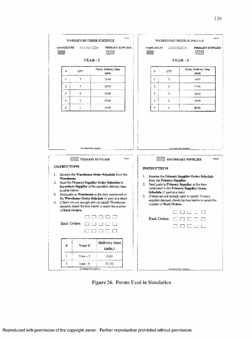
139
WAREHOUSE ORDER SCHEDULE
WAREHOUSE PRIMARY SUPPLIER
Y E A R - 2
# QTYOrder Delivery Time
(aste)
2 11:00
2 3 12:00
3 2 13:00
4 2 14:00
5 I 15:00
.IMARY SUPPLIER
INSTRUCTIONS
1. Receive the Warehouse Order Schedule from theW arehouse.
2. Send the Primary Supplier Order Schedule toSecondary Supplier at the specified delivery time in table beiow.
3. Send parts to W arehouse at the time mentioned in the W arehouse O rder Schedule (I part at a time).
4. IF there are not enough parts to satisfy Warehouse demand, check the box below to count the number o f Back Orders.
Back Orders□ □ □ □ □ □ □ □ □ □□ □ □ n □
I ^
---------------
Year#Delivery time
(mm*)
I 1 Year - 2 6:00
J 2 i Year - 3 11:00
WAREHOUSE ORDER SCHEDULE
WAREHOUSE _ ; . ' ; ' > PRIM ARY SUPPLIER
YEAR-3
# QTY O r f e Delivery Time(Min)
2 16:00
2 3 17:00
3 2 18:00
4 2 19:00
5 1 20:00
SECONDARY SUPPLIER
INSTRUCTIONS
1. Receive the Primary Supplier Order Schedule from the Primary Supplier.
2. Send parts to Primary Supplier at the time mentioned in the Prim ary Supplier Order Schedule (1 part at a time).
3. If there are not enough parts to satisfy Primary supplier demand, check the box below to count the number of B ack Orders.
□ □ □ □ □Back Orders □ □ □ □ □
Figure 26, Forms Used in Simulation
Reproduced with permission o f the copyright owner. Further reproduction prohibited w ithout permission.
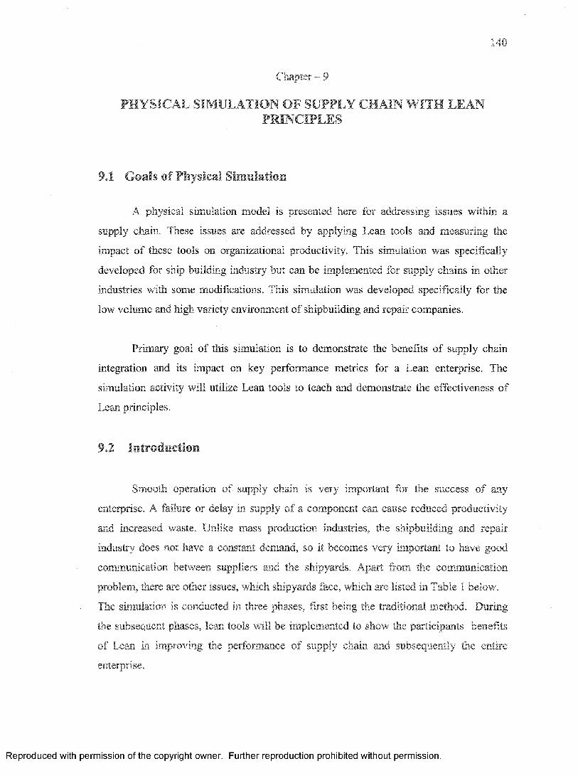
140
Chapter - 9
PHYSICAL SIMULATION OF SUPPLY CHAIN WITH LEANPRINCIPLES
9.1 Goals of Physical Simulation
A physical simulation model is presented here for addressing issues within a
supply chain. These issues are addressed by applying Lean tools and measuring the
impact of these tools on organizational productivity. This simulation was specifically
developed for ship building industry but can be implemented for supply chains in other
industries with some modifications. This simulation was developed specifically for the
low volume and high variety environment of shipbuilding and repair companies.
Primary goal of this simulation is to demonstrate the benefits of supply chain
integration and its impact on key performance metrics for a Lean enterprise. The
simulation activity will utilize Lean tools to teach and demonstrate the effectiveness of
Lean principles.
9.2 Introduction
Smooth operation of supply chain is very important for the success of any
enterprise. A failure or delay in supply of a component can cause reduced productivity
and increased waste. Unlike mass production industries, the shipbuilding and repair
industry does not have a constant demand, so it becomes very important to have good
communication between suppliers and the shipyards. Apart from the communication
problem, there are other issues, which shipyards face, which are listed in Table 1 below.
The simulation is conducted in three phases, first being the traditional method. During
the subsequent phases, lean tools will be implemented to show the participants benefits
of Lean in improving the performance of supply chain and subsequently the entire
enterprise.
Reproduced with permission o f the copyright owner. Further reproduction prohibited w ithout permission.

141
93 Important IssuesThe following table lists the issues related to supply chain that currently plague
the shipbuilding and repair industry. The table below is a general list and is not ranked.
Table 45 lists the Lean tools that could be used to reduce or eliminate the problem.
_ Scheduling Problem Pull, Integrate Planning & Sourcing with suppliers, information sharing
2 Adversarial Relationship with Supplier Team - Sharing information, long-term commitment, communication
3 No Involvement of Supplier in Design. Co-location4 Long Lead-Time Pull, Group technology5 High Costs Batch size reduction.6 High Inventory POUS, Pull, 5S, Batch reduction, TPM7 Challenge in Synchronizing Flow with
Suppliers.Pull, Kanban, Takt time.
8 Vendors Furnishing Information Late Map information flow, (reduce paperwork, improve scheduling)
9 Irregular Performance Built in quality, mistake proofing.10 Higher Price to US Shipyards Co-designing, sharing information, long
term commitment11 Shrinking Choice of Vendors Vendor development12 Many Engineering Changes Concurrent Engineering, Co- location.
Table 45. Issues in Supply Chain and Lean Tools
9.4 Simulation Activity
SUPPLY CHAIN
m m
; psferj SuppSer -JJ Psifeys ar4 Bex
j j i |l ||||||||||||||i i l l l l l l l l l
m
Pham . I
S SupfSilM 1 [ Gngne.aenstator. ‘ : Central , rsoBs, /. ^fspeHsr/ Pmo«slsr . I
/ I
ter? tSfint ,: Sub-Ammbiv :
bfffH jlapp lle r-2
Btsalinaliort Plant, Battery, Crew Compartment
...... I
Assets
Inventor iA . !
Asswih i ii
" su p p ii« --4
Tradittonsi - Push
Figure 27. Room Layout for Phase -I
Reproduced with permission o f the copyright owner. Further reproduction prohibited w ithout permission.

142
The simulation activity will be carried out in 3 phases, first being the traditional
way a typical supply chain operates. Figure 27 above shows the room layout for the first
phase. In the first phase, the participants will encounter the problems faced in a
traditional supply chain like, frequent engineering changes, vendor furnishing
information late, high inventory, material not being received on time, quality problems,
communication problems, long lead times, etc. Problems like machine breakdown and
weather conditions are difficult to show in a simulation, a variability wheel, as shown in
Figure 28, is used at Supplier 1 and Supplier 4 to bring the simulation closer to reality.
Phase-I
■ On-Time■ Non-Availability
of Resources■ Weather
Condition■ Machine
Breakdown
Figure 28. Variability Wheel
In the second phase, Lean is implemented only at the primary suppliers. Due to
implementation of Lean, quality at source is built into the production system. This will
reduce the quality checks on parts sent from primary suppliers to the shipyard. However,
since the secondary suppliers are still not lean, quality check on incoming parts have to
be done at primary suppliers. Additional Lean tools implemented during phase-II include
Total Productive Maintenance and Co-location as shown in Figure 29.
Supply Chain Supplier -1
Reproduced with permission o f the copyright owner. Further reproduction prohibited w ithout permission.

143
5UMH.V CHAWf\% h'S'4*m; l.wu i & '.
I I M B H I I
■ ........ it....ini..............i iiBlii•VWw! : iuppi&riTstipifcri"+ ! Imn&l
j |_ / ' ■ 0®ssgn + P«?«ha»ng& ; !.......^*W*K*i ^ S t J-. . , I..... ....gmtog.......... ]Engnw eawNWer, -PAniMlViftwSwusai ,..
.'. -ri-.v - ,
Cat#*.' ' .■■ :«sis%. j~“ r ’1Pi'spslfsr, Propsfer ,-' Shaft (#ss©mbt®<ii :'<
A /
- 2 L._.Battery, D*saltnatton plant, Crew Compartment
M LWhs
iwsmojy •'£
1■ ■ ■ ~i . '.,Safe-Assewtsiy j f-
" ■ n & z z , j **»«**SulMWaBSy y ---- -
-£5,---_---_ ---.
s ^ m - n --------------Pwpeler Shaft, Battery T«mloal5 Desalination plant
Figure 29. Room Layout for Phase -II
Primary suppliers, and design and planning departments are co-located at the
shipyard, which aids in better communication between the shipyard and its suppliers.
This is illustrated in the Figure 30 below.
fO U'KTTTo^ _ IMPROVED COMMUNICATIONF F tt> ^ XrtpfaMtt l^ f ta s *
{ 53]:;pr^vi }
.^I'feeonciaty 'N
( Shipyardi f l h H H H II;;;:;:;:;:;;:!:;;:;';
/ Primary \ Suppliers
i l l
"v
I,,..Jilll i i s i i l
Shipyard )■ pnPrimarySupplier? 1
pr
Supplier? .,•
Figure 30. Communication through Three Phases
Reproduced with permission o f the copyright owner. Further reproduction prohibited w ithout permission.
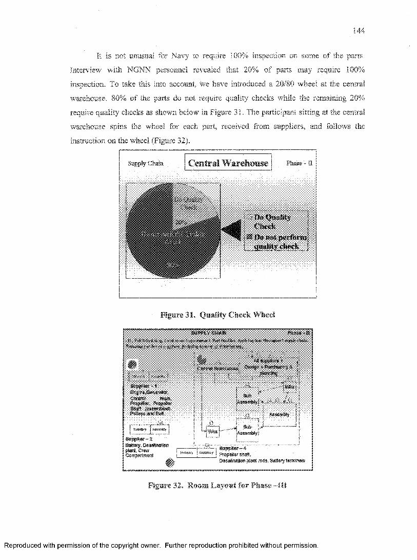
144
It Is not unusual for Navy to require 100% Inspection on some of the parts.
Interview with NGNN personnel revealed that 20% of parts may require 100%
inspection. To take this into account, we have introduced a 20/80 wheel at the central
warehouse, 80% of the parts do not require quality checks while the remaining 20%
require quality checks as shown below in Figure 31. The participant sitting at the central
warehouse spins the wheel for each part, received from suppliers, and follows the
inst.ni.ct.ion on the wheel (Figure 32).
i jsupply chain I Central Warehouse j Pfa* - n
i LJ Do Quality j! Cheek * ij ■
: Do jsot perftirtn.; quality check
Figure 31. Quality Check Wheel
SUPPLY CB*tM Pfea** - IBittt. JM! grta 4«3ng« ? nfttLmtti tap94yiato*a?, Part Appbtag kt&a Huro«i^w*t tfepySy cfoo,
of suppers, mimhm of Wbsrdstmstfs..
mmmsimmiiSafsflier -1 Engfere.Generalor. Centro! raws, Prcff><*w, sopefter Shaft sosseoeted). puwyg andean.
inmiorv jj f M m r n jSappier-2 Battery, Destinationp lan t, C rew |C om partm en t i
1 0 i AiiffippSws*hHttraVferafcausall Dasfon + Pashas#* S j
Iggjigli ■I
■iWhs!;j sub ; SAssamblyl * -i I !
Wrt.rfJ.-i
ASSembJy£wn*i % Sub p
iAstembtyj
~iSrinventory | AssemfeSy
' — 4 P ropeller s M ,D esalina tion p lan t ro d s , B attery te rm ina te
Figure 32. Room Layout for Phase -III
Reproduced with permission o f the copyright owner. Further reproduction prohibited w ithout permission.

145
Daring the third phase, tools like just in time (JIT), and part families will be
implemented, which will reduce the problems associated with high inventory and late
deliveries. Number of suppliers is reduced by forming part families and Lean is applied
throughout the supply chain.
9.5 Model for Simulation
The simulation uses the production and assembly of a submarine and its
associated supply chain to demonstrate the impact of Lean principles. Figures 33-35
illustrate the submarine model and its various components. The model has been designed
to replicate the details of construction of an actual submarine. The assembly sequence
and construction activity closely mimic the actual process.
Figure 33. Submarine Model Components
Figure c .. Aft Component
Reproduced with permission o f the copyright owner. Further reproduction prohibited w ithout permission.

146
Figure 35. Assembled Submarine Model
The model consists of 3 hulls, a nose, an aft and a conning tower forming the
exterior of the submarine. The hull components can be seen in Figure 33 and the final
assembly is shown in Figure 35. There are two sub-assembly stations where different
components like engine, generator, control room, battery, crew compartment,
desalination plant and torpedo compartment are assembled in the Hull. The participants
will be provided with pictorial instructions to aid in assembly.
9.6 Implementation of Simulation Activity
The simulation activity requires approximately 18 participants with each person
having a role to play in the supply chain simulation. The 3 phases are not time bound and
the activity will continue until the first Submarine model is built. The time required
during the first phase is higher compared to successive phases. At the end of each phase,
participants are encouraged to discuss the problems encountered during simulation and
these issues are noted down. During the following phase a set of Lean tools are
implemented. The simulation demonstrates to participants, how application of simple
Lean tools can benefit the enterprise. Participants observe that Lean when applied
Reproduced with permission o f the copyright owner. Further reproduction prohibited w ithout permission.
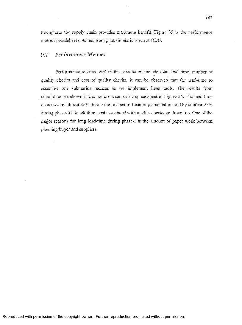
147
throughout the supply chain provides maximum benefit. Figure 35 is the performance
metric spreadsheet obtained from pilot simulations run at ODU.
9.7 Performance Metrics
Performance metrics used in this simulation include total lead time, number of
quality checks and cost of quality checks. It can be observed that the lead-time to
assemble one submarine reduces as we implement Lean tools. The results from
simulation are shown In the performance metric spreadsheet in Figure 36. The lead-time
decreases by almost 46% during the first set of Lean implementation and by another 25%
during phase-III. In addition, cost associated with quality checks go down too. One of the
major reasons for long lead-time during phase-! is the amount of paper work between
planning/buyer and suppliers.
Reproduced with permission o f the copyright owner. Further reproduction prohibited w ithout permission.

148
PERFORMANCE METRICS - SUPPLY CHAIN
PEftFGRMAHO: C R IT im ll llf lllll Phase i l i l l i l l im m m m m m m a r n 19 f " 1\ tad r ify,s if a cc'TifihS? ifne snsrj omit,) ...........................
35 19 15Tolas mjmhe» of Quaiil* Checks 25
_ _2
1 >' Ossf if OtldbiT cfiE'U58
me50 1
1 — —50100 f
fcwens-i'.v Cofi
OfCLE TIME 6ntn.)Planning m 4.5 3.5Primary Suppiiw -1 32 SJ 5 JPrimary Supplier-2 6.0 42 4.0Central Warehouse 5J 2.1 2.0Sub-Assembly -1 5.0 2.5 2 JSub-Assembly -2 5.6 3.8 I SAssembly 5J 3J0 2 J
Cycle Tim© Cdnpainkm
Phase4.0 ■Phase
L®*f itane ComiHrtrian
| 30 -
I 20 - M............. ...............latesdThiej
| 10 -
■J o - ■ ■ i j1 2 3
Simulation W as® tteM*er
Number of QuaOly C tecics
# ai i j i tr |h # of GuaSy Ched® |
I D '“ t l % u —.... | j ................
1 2 3Simulatiton M wse Somber
Total eo a t of €
1500 -
1000 H S Total Cost of Gualy Checks
Figure 36. Performance Metrics Spreadsheet from Pilot Session
9.8 S u m m a r y
Physical simulations are powerful tools for demonstrating effectiveness of Lean
principles and tools on the productivity of an organization. The results discussed in the
previous section show a consistent decrease in the total lead time, cycle time at stations
and cost of quality control. The simulation also demonstrated the effectiveness of Lean
tools in streamlining the supply chain. This can be critical for a large organization with
long supply chains involving multiple tiers. While the physical simulation in chapter was
specifically designed to demonstrate the Base Stock model, this simulation shows the
supply chain for submarine construction.
Reproduced with permission o f the copyright owner. Further reproduction prohibited w ithout permission.

149
Results shown in Figure 36 show that lead-time reduces as we go from phase-I to
phase-III. This happens due to implementation of different lean tools. The drastic
reduction in cycle time for buyer/planner is due to better communication in the second
phase, which is brought about by co-locating the suppliers with the shipyard. Number of
quality checks decrease and correspondingly the cost of quality checks also goes down,
due to implementation of quality at source at the primary and secondary suppliers.
Reproduced with permission o f the copyright owner. Further reproduction prohibited w ithout permission.

150
Chapter - 10
COMPUTER BASED SIMULATION MODEL
Computer based simulation is the “imitation o f a dynamic system using a
computer model in order to evaluate and improve system performance” [64]. In practice,
simulation is usually performed using commercial simulation software like ProModel that
have modeling constructs specifically designed for capturing the dynamic behavior of
system. Performance statistics are gathered during the simulation and automatically
summarized for analysis. Modem simulation software provides a realistic, graphical
animation of the system being modeled. During the simulation, the user can interactively
adjust the speed and model parameter values to do a “what i f ’ analysis. Some simulation
software provide optimization technology also. Trial and error approaches are expensive,
time consuming and disruptive. The power of simulation lies in the fact that it provides a
method of analysis that is not only formal and predictive, but is capable of accurately
predicting the performance of even the most complex systems.
The terms continuous and discrete applied to a system refer to the change of state
of the system with respect to time. A system whose changes in state occur in finite quanta
or jumps are known as discrete systems [65], Supply chains are discrete systems since a
customer order triggers the change of state in these systems.
A discrete event simulation model is created using ProModel software to assess
the performance of a two tier supply chain. Base stock Model and (Q, r) Model were
applied to this supply chain in the previous sections.
10.1 G o a ls of Computer Based Simulation
Primary goal of this computer based simulation is to demonstrate that Base Stock
Model can effectively predict the level of inventory at reorder point. Another goal is to
compare the results obtained here with those of mathematical model and physical
simulation model.
Reproduced with permission o f the copyright owner. Further reproduction prohibited w ithout permission.
151
10.2 Software Used
Pro-Model is a computer simulation program that allows its user to evaluate the
effectiveness of a given process, Pro-Model utilizes the Windows graphical interface to
make programming more user-friendly [62, 63], Components of this process can be
rearranged to optimize productivity. This allows for many changes in the simulation
before anything is installed or moved physically. To create this simulation several
parameters need to be specified. Locations, entities, processes, resources, and arrivals
must be specified for the program. Entities are the items being processed. Locations are
defined as the various areas where work is being done to the entities or the entities are
being stored. Processing is the route in which the entities travel and the logic behind that
travel path. Resources are the personnel and equipment used for the process, and arrivals
are the number and frequencies of additional entities to the process. The finished model
can then be simulated using animation.
After the initial conditions are specified, more detail is needed to make the
simulation realistic. This software has the capability of simulating work done in shifts,
which also encompasses breaks for the employees and down times for the equipment. A
few additional capabilities of ProModel include programmable times, distributions and
cost analysis.
10.3 Simulation Layout
Discrete event simulation is a pedagogical tool that uses computer models to
study a production system with the goal of optimizing its performance. ProModel
simulation software is used for analyzing and assessing the flow of parts through a two
tier supply chain system. A computer model of a two tier supply chain was build using
ProModel software. The model uses four locations to indicate the key players in the
supply chain namely Customer, Ware House, primary Supplier and Secondary Supplier.
The layout of the model is shown in Figure 37.
Reproduced with permission o f the copyright owner. Further reproduction prohibited w ithout permission.
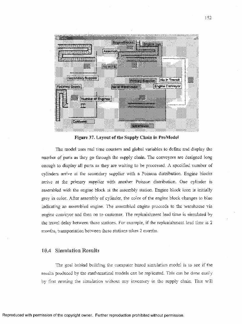
jAssembivl
^Sa^^WiteBBiiirtr...
| } j I . .f-Ji.ttit'ier ti‘ iU-girK;
nr. v .V8teh0U5»
■m -
■ t.uswre. ;
Figure 37. Layout of the Supply Chain in ProModel
The model uses real time counters and global variables to define and display the
number of parts as they go through the supply chain. The conveyors are designed long
enough to display all parts as they are waiting to be processed. A specified number of
cylinders arrive at the secondary supplier with a Poisson distribution. Engine blocks
arrive at the primary supplier with another Poisson distribution. One cylinder is
assembled with the engine block at the assembly station. Engine block icon is initially
grey in color. After assembly of cylinder, the color of the engine block changes to blue
indicating an assembled engine. The assembled engine proceeds to the warehouse via
engine conveyor and then on to customer. The replenishment lead time is simulated by
the travel delay between these stations. For example, if the replenishment lead time is 2
months, transportation between these stations takes 2 months.
10.4 Simulation Results
The goal behind building the computer based simulation model is to see if the
results produced by the mathematical models can be replicated. This can be done easily
by first running the simulation without any inventory in the supply chain. This will
Reproduced with permission o f the copyright owner. Further reproduction prohibited w ithout permission.
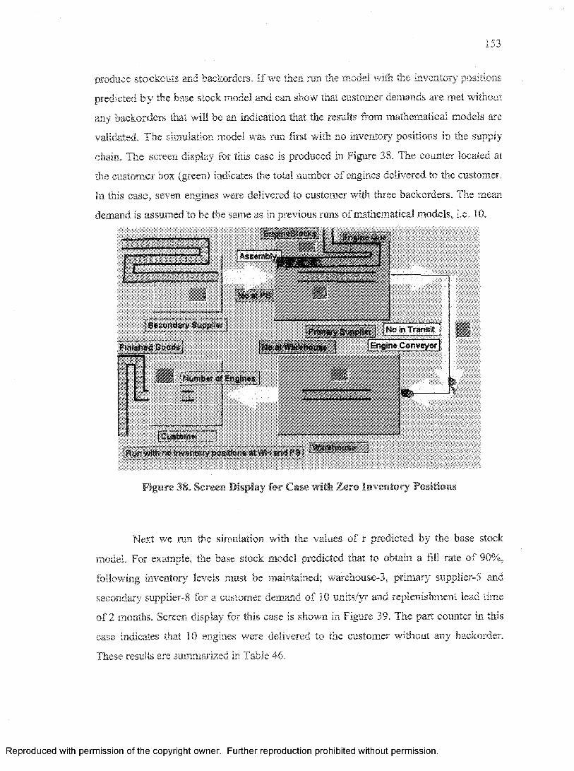
153
produce stockouts and backorders. If we then run the model with the inventory positions
predicted b y the base stock model and can show that customer demands are met without
any backorders that will be an indication that the results from mathematical models are
validated. The simulation model was ran first with no inventory positions in the supply
chain. The screen display for this case is produced in Figure 38. The counter located at
the customer box (green) indicates the total number of engines delivered to the customer.
In this case, seven engines were delivered to customer with three backorders. The mean
demand is assumed to be the same as in previous runs of mathematical models, i.e. 10.
3
1
AS; . i t r a j i a rswnblyw—. mm
pfO E aui.. ■ .
Wat PS; m; Secondary
Finish**? GoodSj
j Primary Suppiier | ! !^jP.7rsr s*• Ho at Warehouse j OTjritCopveyor
j■ I '■'ijmherofesigi-ie’S s ■
ttiiMfflftLTOWiLr ;
j Run with no inventoryposltloris st¥Wj and PS j ^ —3
Figure 38. Screen Display for Case with Zero Inventory' Positions
Next we run the simulation with the values of r predicted by the base stock
model. For example, the base stock model predicted that to obtain a fill rate of 90%,
following inventory levels must be maintained; warehouse-3, primary supplier-5 and
secondary supplier-8 for a customer demand of 10 units/yr and replenishment lead time
of 2 months. Screen display for this case is shown in Figure 39. The part counter in this
case indicates that 10 engines were delivered to the customer without any backorder.
These results are summarized in Table 46.
Reproduced with permission o f the copyright owner. Further reproduction prohibited w ithout permission.

154
■
i Assembly-. ' "***“
■
J |J j |. / * ■.-••• Conveyor] j
M f tNumber of Engines |
«*■*
i Customer
wrrtory posfflonsatWHand PS .Base”$tock!
Figure 39. Screen Display for Case with Inventory Positions per Base Stock Model
Case Inventory at FS/.
Inventory atW B
Lead time Engines to1 ;;
Number ofBadkttfdtrs' ■
1 0 0 60 days 7 32 r s 3 60 days 10 0
Table 46. Results from ProModel
Table 46 shows the inventory levels and number of engines produced during the
two cases for lead time of 60 days. Customer demands are met with no backorders when
predicted values of inventory position are used.
ProModel software can generate a number of tables and charts to analyze a
simulation model. A few of these tables and charts are discussed here. Table 47 shows all
the locations defined within the model and their state. It also indicates average content,
maximum content and % utilization at those locations. Table 58 shows the percentage
utilization of multi capacity locations. This is used to determine % empty, % occupied
and % full state of these locations.
Reproduced with permission o f the copyright owner. Further reproduction prohibited w ithout permission.
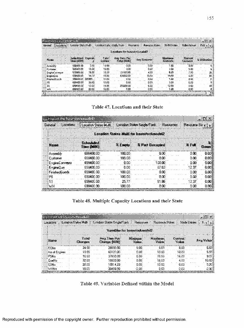
155
flew^nm ; Lnrtfior. QMta VtMt l.'X-u&-nSE6!*i;r,f fe.. f .» . H e w s ; . SefcAs.s S«®', iiKhkf&r-. Er f $ s j # | j
I nfcahBiw im H*i»s?otij»»<feR‘ieteisstesS- Ds|»sii ■v - i i i ia i- ' &«<S T«bb Vet Ars SAfitenis 7' Ummmm Sersajsi.wHiiuno g F«aw tm f. ■ .. . ■ -. t.MtU&zt’i
|AssaTfc|i ^wSSSncr^”... f S f .... ..'"“'5m" am. 1.00: smICmtoBW mm. m 18.00 io.m aoo o.t» 1.00 3.80j EngtreCotwsyot 698400.00 18.00 16.00 197550.00 453 8.00 .......... 7.6b;jjEngjnsQue 63®4e&f» 18.00 18.00. 424030.00 m ss m m 4.00I FrisheidEiooch S98400.00 S3S389... 10.00: ' 0.00 ....................am 1.00 am"jPS " 838400.00 a m ....... 18.00: 0.00 0.00 ' zoo aooIS5 6«3*0«? 12.00 14 90 m m m 5.20 ' 12.W " 009"avh 538400 00 20 CG 10.00 0.00 0.00 1.00: : :
IS 1
' a| 25.J
m|" a |aj
*;its*
Table 47. Locations and their State
C:sr.e;el : .9":.30<y-:i i Loc?.l:cr : la*e<t w.ulli ; oce?HJf. States Sir-jie/T er.'
Name
Assembly Customer EngineConveyar
. EngineQue FinishedGoods
PS.S3WH
fimmjtvm
i.ncatHJ*-- 3tate* fcSulifE toy iiesestcorracdd?
s J S J?lRe'irv.v-.-e =>i i >
Scheduled 1 one (MIN)
638400. OG SS8400.0G538400.00698400.00 698400.0G698400.00698400.00698400.00
% Empty % Part Occupied SFuSi XDown
10G.G0 0.00 0.00 0 00100.00 0.00 0.00 0.00
0.00 100.00 0.00 0.000.00 37.63 12.37 dm
100.00 0.00 0.00 0.00109.00 0.00 0.00 0.00
25.77 61.86 12.37 0.00100 GO ............................0.00 ....... 0.00 "0.00
Table 48. Multiple Capacity Locations and their State
leestons - L<»##or. S t*» Mufi t ocstion Stela* Singfe/T ank 1 Resource* Flesoisse Slate • Node Enbisc ?. *;*{(
Variables lot basestodkmodeiS:
Hast®
If-c•S
ECNoNo of Engines
}PSNo GueNo SSNo WHNo
: t i i i l T " A ifgltw sPffii MiratnutB Manwun CwFmnlChanges ' ■ 'e f e w p ip i i i i ' ' Value Value
24.00 " " 20830.00 0.00 ' 9.00"" aoo’ 10.00 .......... 63120.00 0.00 ..........10.00 ■ " 10.001S.00 ' 37800.00'" ' 0.00 16.00' 16.00:32.00 18900.00 0.00 18.00 4.0028.00 18514.29 0.00 12.00 0.0018.00 38400.00 -2.00 0.00 -2.00
AvgVaicw5.53 5 35 3 07
10.93 5.201 -2.001
Table 49. Variables Defined within the Model
Reproduced with permission o f the copyright owner. Further reproduction prohibited w ithout permission.

156
Table 49 shows the data for all variables used within the model. This table is used
to obtain the minimum, maximum, average and current value of a variable. Figure 40 and
41 show the time plot of these variables throughout the entire simulation time period.
These charts help us debug the simulation by charting the simulation progress.
■ '»».€<■ Q . m is ;t.„i, • %Cto&wte .'hfisfc/saut fhfco v*t»«HsUv txx&r&t -• %;&*&&& tusrxxUs
1800 J# JGdO&j VSfcBOh 9*10 BD 7lJ0f},C*J 30SJJ1& 9Q&ao VttQOjOQ TIGQO&f 12O0OHv-jfi.
Figure 40. Time Line for Various Variables
1 tW W.*-Klb-'S’I <»■*?>ur& : <g> q * - . 4 ‘ js m m : L L. r* C.-ji p. '*<•SS witarite SS VafoeHfeftsy
P5N3 Value Hb&»y •Wcorirtrta
GJuesftoVa&Hwtorv.VdwaWdary
'jam tsao Si&-
14 00
...
.4*0~r>&3SfiC■i *.dJs3
Figure 41. Time Line for Various Variables
Reproduced with permission o f the copyright owner. Further reproduction prohibited w ithout permission.

157
' m[ & f i 0 Q
: £J % 6"***
?0 .
tF IB L L :%
C * Pw* OtSt**K* O % Fu»
Assemfeiy ■ ...■ j
; EngreCcnveyo*'
Ss® w.o.. o , i . '- .o v:,;:; jc . ./ . ,'c.-tj tr:-.-. u •:■:■
Figure 42. State C hart for Locations
■: *4 J * : O M i : L j L . . «af l % Ufeatton
0.00 10.00 20.00 SB .00 40.60 33,00 80.00 ?GjO0 6C.0G 90.08 1«Xi»Pwceri
Figure 43. Percent Utilization Chart
Figure 42 shows the state chart for all locations defined within the simulation.
This chart indicates % foil, % empty and % occupied status of all locations. Figure 43
shows the % utilization of a few specific locations. Figure 44 is similar to Figure 42.
except it is for entities.
Reproduced with permission o f the copyright owner. Further reproduction prohibited w ithout permission.

158
H , ; t t x,(Mi * i | | § Q ; £■ V i *S S | .70* iff! £ U lS :;:
] rih =r> &ov*b ^ Fa? rig-S f"j % ‘ft U j^ d w e n tw
':" ' ■'" .. ‘"" - ■• ■_ - . - ., .. .... ( ... ,-.«.••• i*' I!5.m 30 00 40 00 SO 00 f'O 00 1 on 00 )
. . . . ,.; .......
Figure 44. Entity States of Engine and Engine Block
10.5 Summary
Computer based simulation model is created using ProModel software to assess
the values of inventory levels predicted by base stock model. Creation of a simulation
model requires a detailed understanding of the process. Common elements of a
simulation model are locations, entities, processing, arrival, variables and attributes etc.
Once a model is built using these elements, its validity is checked by running a few trial
cases. Results from the computer simulation model validate the results predicted by base
stock model. This was done by first running the simulation with no inventory positions
either at the primary supplier or the warehouse. This resulted in backorders. Then the
primary supplier and warehouse were populated with inventory positions predicted by the
base stock model The simulation model showed that all 10 engines were delivered to the
customer without any backorders.
Reproduced with permission o f the copyright owner. Further reproduction prohibited w ithout permission.

159
Chapter - 11
DISCUSSION ON RESULTS
Published work in the area of supply chain covers a plethora of topics which are
outlined in chapter 5. Specific issues related to supply chains of shipbuilding and repair
industry are discussed in section 3,1 of chapter 3. Mathematical models clearly show that
the total cost of inventory can be brought down by reducing replenishment times and
increasing the frequency of replenishments. The cost associated with ordering is more
than compensated by benefits due to added flexibility from a reduction in replenishment
lead times.
Physical simulations models discussed in chapter 10 clearly indicates the benefits
of implementing lean through reduction of the lead time and increased flow through the
supply chain. This simulation is brought closer to the stochastic and dynamic nature of a
supply chain by introducing variability due to weather, machine breakdown, non
availability of resources etc. During phase II, Lean is implemented only at the first tier of
the supply chain. This is extended to second tier in phase III. Principles of concurrent
engineering are incorporated in phase II by requiring the suppliers to meet with
buyer/planner of the company during phase II and III. The results of these
implementation lead to a consistent reduction in cycle time for all seven workstations.
Total lead time goes down from 35 to 19 to 15 minutes. Total cost of quality checks goes
down from $1250 to $550 to $100.
The physical simulation model for Base Stock discussed in chapter 9 was used to
validate the inventory levels for reorder point as predicted by the mathematical model
The optimum level of inventory when used with the simulation did not result in any
backorder. When these levels were reduced, backorders were observed confirming the
results of the mathematical model. The results of the mathematical models are discussed
below.
Reproduced with permission o f the copyright owner. Further reproduction prohibited w ithout permission.

160
The Base Stock and (Q, r) inventory control models are compared for different
replenishment lead times. If we compare the results from table 23 (Base Stock Mode!)
and table 39 ((Q, r) model), there is a significant decrease in the frequency of order in (Q,
r) model as compared to Base Stock model. The two tables are reproduced here for
convenience. The frequency of order plays an important role here, as there is cost
associated with placing the order. Replenishment at higher frequency however, may be
beneficial from the point of customer satisfaction and Lean implementation. Higher
frequency of replenishments also helps the organization become more agile in meeting
customer demand.
RepleitbliineaiIJftteswd
Steanfcrq . . zA'A&hlM'e
Frequency ofortter (P=I)/Q)
AverageDmwmhI :
O rderC«9t
TutsiCiftSt
1210 14.00
1.00Warehouse 10.00 10 250 925
14 19.00 PS 14.00 14 350 117519 25.00 s s 19.00 19 475 1450
86.67 10.00
1.00Warehouse 6.67 6.67 166.75 741.25
10 14.00 PS 10.00 10 250 92514 19.00 SS 14.00 14 350 1175
610 8.00
1.00Warehouse 10.00 5 250 775
16 11.00 PS 16.00 8 400 92522 15.00 SS 22.00 11 550 1225
410 6.00
1.00Warehouse 10.00 3.33 250 725.5
18 9.00 PS 18.00 6 450 975
27 13.00 SS 27.00 9 675 1350
21.67 3.00
1.00Warehouse 1.67 1.67 41.75 316.25
3 5.00 PS 3.00 3 75 4505 8.00 SS 5.00 3 125 950
Table 23. Summary of Results Application Runs of Base Stock Model
The Base Stock model emphasizes on replenishment quantity of 1 and therefore
has higher frequency of order. On the other hand, the (Q, r) model provides a lower total
cost, since the frequency of order is less. The service factor obtained for (Q, r) model is in
the range of 0.94 - 0.98, which falls within an acceptable range for most organizations.
The service factor for Base Stock model was assumed to be 90%.
Reproduced with permission o f the copyright owner. Further reproduction prohibited w ithout permission.

Tis■KxsiS”
S
a” 'jsuqfw*
•viW
-
: ' ■■ ' ...
■
b
&S}p? W 2 i
<w
2.00
■
'•j* ^" ' "S' I: g m.
;> 3 < Ct
asa &35Wat,& V
$ wi i« y £ ^
■
:*h*. o,*VV'
" ' A * # 1'mV :
15.
12 WH 0.32 13.00 5.00 0.94 10 825 25.6 50.00 900.60PS 0.44 16.00 7.00 0.94 1.86 13 975 32.7 46.43 1054.10SS 0.37 20.00 7.00 0.95 2.29 16 1125 33.8 5 7 .1 4 ^ 1216.00
6 WH 0.26 7.00 4.00 0.94 2.50 5 600 26 62.50 688.50PS 0.20 10.00 6.00 0.97 2.33 7 900 18.7 58.33 977.00SS 0.19 14.00 7.00 0.97 2.86 10 1125 21.7 71.43 1218.10
2 WH 0.13 3.00 4.00 0.97 2.50 1.67 499.5 13 62.50 575.00PS 0.13 5.00 6.00 0.98 3.00 3 750 15.6 75.00 840.60SS 0.12 8.00 8.00 0.99 3.75 5 1050 18 93.75 1161.80
8 WH 0.29 9.00 5.00 r~0.94 2.00 6.67 724.5 23.2 50.00 797.70PS 0.28 12.00 6.00 0.95 2.25 9 900 25.2 56.25 981.50SS 0.25 16.00 7.00 0.96 2.57 12 1125 25.7 64.29 1215.00
4 WH 0.21 5.00 5.00 0.96 2.00 3.33 625.5 16.8 50.00 692.30PS 0.12 8.00 5.00 0.98 3.00 5 825 14.4 75.00 914.40ss 0.24 1 1 . 0 0 8.00 0.97 3.00 8 1050 28.8 75.00 1153.80
Table 39. Summary of Application Runs for (Q, r) Model
Reproduced with permission o f the copyright owner. Further reproduction prohibited w ithout permission.

162
Chapter - 12
CONCLUSIONS
An efficient supply chain is one which can deliver the right amount of product at
the required place at the right time in spite of the variability and supply chain dynamics.
Deterministic models fail to take into account system variability and thus are inadequate
for modeling complex supply chain systems. Deterministic models however, are certainly
useful in cases where demand is relatively well known and fixed.
The Base Stock model has been widely studied in the operations management
literature and it is simple to analyze. This model assumes that demand occurs one at a
time in quantity of one. It also assumes that lead times are known and fixed and there are
no setup costs associated with orders. This model provides us with a value of inventory
level r for a certain customer satisfaction level or fill rate. In general, the higher the mean
demand during the replenishment lead time the higher the value of r to achieve a
particular fill rate. In addition, the variability of the demand also affects the value of r.
The higher the standard deviation of demand , the larger the value of r. In this model,
reorder point controls the probability of stockouts by establishing a safety stock.
In (Q, r) model, the replenishment quantity Q affects the tradeoff between order
frequency and inventory. Large values of Q will result in fewer replenishments per year
but will produce higher level of average inventory. Smaller values will produce low
average inventory but higher frequency of replenishments. The reorder point r, affects the
probability of a stockout. A high value of r will produce higher average inventory but
lower probability of stockouts. A lower value of r will produce higher probability of
stockouts. Thus, these two variables generate two different kinds of inventory. Q affects
the cycle stock: inventory held to avoid excessive replenishment costs. The reorder point
r affects the safety stock: inventory held to avoid stockouts.
In summary, the two mathematical models discussed here adequately capture the
variability in the supply chain. However, they have limitations due to the assumptions
Reproduced with permission o f the copyright owner. Further reproduction prohibited w ithout permission.
163
they make, Some of these assumptions provide a scope for future developments in
modeling.
Physical simulations also capture system variability for a complex system and
often provide a simple method for demonstrating complex ideas. Two physical
simulations were designed and developed. One to specifically simulate the Base Stock
model and validate results obtained. The second one to simulate a two tier supply chain
system for submarine construction. The second model also demonstrated the impact of
Lean tools on supply chain integration.
The computer based simulation model using ProModel software validated the
results from the base stock model by indicating that if quantities of base stock level axe
selected correctly, it can enhance the flow through a supply chain and maximize customer
satisfaction. This can be a formidable tool in the hands of inventory managers who
constantly struggle to find the right compromise between minimizing inventory and
maximizing customer satisfaction.
In summary this dissertation aims at demonstrating the validity of two
mathematical models, namely Base stock and (Q, r) through the applications of physical
simulation and computer based simulation models. It also generates a number of practical
recommendations for the inventory control managers. These recommendations are:
1. Use computer simulations to explore the dynamics of a supply chain. This
recommendation is particularly relevant when the supply chain is very
complex and the user desires to explore many ‘what - i f scenarios.
2. Use physical simulations to explore the impact of implementing lean. This
approach requires some initial investment in capital and time but the
benefits derived in convincing the management and long term benefits
from implementation will far outweigh the initial investment.
3. Given the validity as provided by both physical and computer simulations,
the simple Base stock and (Q, r) models should be used as a first-hand
Reproduced with permission o f the copyright owner. Further reproduction prohibited w ithout permission.

164
approach to determine the order quantity (Q) and reorder point (r) and the
safety stock.
Reproduced with permission o f the copyright owner. Further reproduction prohibited w ithout permission.
165
Chapter - 13
CONTRIBUTIONS OF PRESENT RESEARCH WORK
Scope of Research
• A survey of existing deterministic and stochastic models for inventory control
was conducted.
• Two stochastic mathematical models were implemented for a two tiered
supply chain.
• Design and development of physical simulation model to simulate Base Stock
model.
• Design and development of a physical simulation to demonstrate the effect of
Lean principles on supply chain integration.
• Design and development of a discrete event simulation model for two tiered
supply chain using ProModel software.
• Comparative analysis of results from the above three types of models.
® Demonstrate the effect of lean tools using physical simulation on the
effectiveness of supply chain in shipbuilding and repair companies.
• Use of all three types of tools to study the supply chain integration problem.
Future Work
• Application of these models to multi-product supply chains.
• Design and development of physical simulation model to simulate (Q, r)
model.
• Design and development of a discrete event simulation model using ProModel
software to study (Q, r) model.
• Comparative analysis of results from the above two models for a three tiered
supply chain.
Reproduced with permission o f the copyright owner. Further reproduction prohibited w ithout permission.
166
• (Q, r) model makes the assumption that replenishment lead times are fixed
and known, demands occur one at a time and that each replenishment order
has a fixed cost. In reality these assumptions are not true and a model should
capture these sources of variability.
• A software tool can be developed for inventory managers which will provide
the optimum values for reorder point and order quantity for a given lead time
and customer satisfaction level.
Reproduced with permission o f the copyright owner. Further reproduction prohibited w ithout permission.
167
REFERENCES
1. Womack, James P. & lories, Daniel T. “Lean Thinking”, Simon & Schuster, January, 1996.
2. Executive Review, “Transitioning to Lean Enterprise: A Guide for Leaders” Volume-I, Massachusetts Institute of Technology, 2000.
3. Liter, Jeffrey, “Becoming Lean” Productivity Press, February, 1998.
4. Womack, James P., Jones, Daniel T. and Roos, Daniel “The Machine That Changed the World, Harper Perennial, New York, NY, 1991.
5. Schonberger, Richard, “World Class Manufacturing: The Next Decade”, Free Press, May, 1986.
6. Conner, Gary, “Lean Manufacturing for the Small Shop”, Society of Manufacturing Engineers, 2001
7. Allen, John, Robinson, Charles and Stewart, David, “Lean Manufacturing a Plant Floor Guide”, Society of Manufacturing Engineers, 2001
8. Feld, William, “Lean Manufacturing, Tools, Techniques, and How to Use Them”, The St. Lucie Press, 2001
9. Proceedings of the International Lean Manufacturing Conference, Lexington, KY, May 2002.
10. Proceedings of the Lean Shipbuilding & Ship Repair Forum, Lexington, KY, June 2002 .
11. Wincel, Jeffrey P., Lean Supply Chain Management: A handbook for strategic procurement, Productivity Press 2004.
12. Copacino, William C., Supply Chain management The Basics and beyond, The St. Lucie Press/ APICS Series on Resource Management, 1995
13. Cooper, Robin and Slagmuider, Regine, Supply Chain Development For The Lean Enterprise, The IMA Foundation For Applied Research, Inc, Productivity, Inc, 1999
14. Handfield, Robert B., and Nichols Jr., Ernest L., Introduction to Supply Chain Management, Prentice-Hall, Inc, 1999
15. Ayers, James B., Supply Chain Project Management, St. Lucie Press, 2004.
Reproduced with permission o f the copyright owner. Further reproduction prohibited w ithout permission.

168
16. Fredendall, Lawrence D. and Hall, Ed , Basics of Supply Chain Management, The St. Lucie Press/ APICS Series on Resource Management,
17. Jones, Mason, R. and Towill, D.R., Information Enrichment: designing the supply chain for competitive advantage. Supply Chain Management. Bradford: 1997. Vol. 2, Iss. 4; p. 137
18. Childerhouse, Paul and Towill, Denis R„ Simplified material flow holds the key to supply chain integration. Omega, Feb 2003 v31 il pi 7(11)
19. Bowersox, Donald J., Closs, David J., Stank, Theodore P. and Keller, Scott B., How Supply Chain Competency Leads to Business Success. Chain Management Review, Sept 2000 volume 4, issue 4, p70.
20. Hopp, Wallace J. & Spearman, Mark L., Factory Physics 2nd Edition, Irwin McGraw-Hill, 2000.
21. Askin, Ronald G. & Goldberg, Jeffrey B., Design and Analysis of Lean Production Systems, Wiley, 2001.
22. Akkermans, H., Bogerd, P., Yucesan, E., and Van Wassenhove, L. N.; “The impact of ERP on supply chain management: Exploratory findings from a European Delphi study”, European Journal of Operational Research; June 2002.
23. Duffey, Mike; “How Gillette cleaned up its Supply Chain” Supply Chain Management Review; Apr 2004.
24. Villa, Agostino; “Introducing some Supply chain Management problems”; International Journal of Production Economics; ‘2001
25. Herrmann, Jeff & Hodgson, Brian; “SRM: Leveraging the supply base for competitive advantage”; SMTA International Conference; October 2001
26. Softchain; “Improving Extended Supply Chain Performance Through Better Control”; June 2002.
27. Quayie, M; “Supplier development and supply chain management in small and medium size enterprises”; International Journal of Technology Management 2002 .
28. Rakotobe-Joel, Thierry, Zbib, Imad, Bakhtiari, Claudia; “Information Systems Failure and Its Impact on the Supply Chain Decision Process”; Decision Sciences Institute, 2002
29. Yang, B. and Bums, N.; “Implications of postponement for supply chain”; International Journal of Production Research, 2003
Reproduced with permission of the copyright owner. Further reproduction prohibited without permission.
169
30. Jordan, Michael S., “Lean Transformation of the Widget Company” ITtoolbox Supply Chain Management Knowledge Base, 2002
31. Bowman, Robert J. , Ford: How to maintain a 10,000-Mile Supply Line, Keller International Publishing, July 200.
32. Global Logistics & Supply Chain Strategies; Ideas & Trends in Supply-Chain Management, May 2004.
33. Murphy, Jean V., “ERP Vendors Expand Offerings, Make Inroads into SCM”, Market Global Logistics & Supply Chain Strategies, December 2003.
34. Friscia, Tony; “The Ideal Supply Chain is within reach; AMR Research”; http://www2.cio.com/anafyst/report2684.htmI, May 2004.
35. MIT, Make-To-Order vs. Make-To-Stock: The role of inventory in delivery-time competition, Working Paper No. 2000-88, Sloan School of Management, 1987.
36. Lee, H.L., Padmanabhan, V., and Whang, S., (1997a), Information distortion in a supply chain: The bullwhip effect, Management Science, 43(4), pp546-558.
37. Lee, H.L., Padmanabhan, V., and Whang, S., (1997b), The bullwhip effect in supply chains, Sloan Management Review, Spring, pp93-102.
38. Hax, A.C. and Candea, D., (1984), Production and Inventory Management, Prentice Hall, Inc., pp216-234.
39. Fogarty, Donald W., Blackstone, John H. and Hoffmann, Thomas R. Production & Inventory Management, South-western Publishing Co., ppl-4, 1991.
40. Oden, Howard W., Langenwalter, Gary A. , and Lucier, Raymond A., Handbook o f Material & Capacity Requirements Planning, McGraw-Hill, Inc., ppl3-15, 1993.
41. Nguyen, V., (1998), A multiclass hybrid production center in heavy traffic, Operations Research, 46(3), S13-S25.
42. Wang, S. and Yu, W.S., Supply chain positioning strategy integration, evaluation, simulation, and optimization, International Conference on Computers and Industrial Engineering, Nov, 2001, Canada
43. Forrester, J.W, (1961), Industrial Dynamics, Productivity Press, Portland, Oregon, ppl3-48.
44. Sterman, J.D., (1989), Modeling managerial behavior: misperceptions of feedback in a dynamic decision making experiment, Management Science, 35(3), pp321- 339.
Reproduced with permission of the copyright owner. Further reproduction prohibited without permission.

170
45. Sterman, J.D., (1995), The beer distribution gome, Gomes and Exercises for Operations Management, Prentice Halt, Englewood Cliffs, NJ, pp 101-112.
46. Goodwin, J.S. and Franklin, S.G,, (1994), The beer distribution game: using simulation to teach systems thinking, Journal o f Management Development, 13(8), pp7-15.
47. Metters, R., (1997), Quantifying the bullwhip effect in supply chains, Journal o f Operations Management, 15, pp89-100.
4 8 . Towill, D.R., ( 1 9 9 6 ) , Industrial dynamics modeling of supply chains, International Journal o f Physical Distribution and Logistics Management, 2 6 ( 2 ) ,
p p 2 3 - 4 1 .
49. Towill, D.R. and McCullen, P., (1999), The impact of agile manufacturing on supply chain dynamics, The International Journal o f Logistics Management, 10(1), pp83-96.
50. Song, Z.C., (1999), Multi-Flow Coordination in Electronics Manufacturing Supply Networks, Ph.D final thesis, Nanyang Technological University, Singapore.
51. Fransoo, J.C. and Wouters, M.J.F, (2000), Measuring the bullwhip effect in the supply chain, Supply Chain Management, 5(2), pp78-89.
52. Chen, F., Drezner, Z., Ryan, K.J., and Simchi-Levi, D., (2000), Quantifying the bullwhip effect in a simple supply chain: The impact of forecasting, lead times, and information, Management Science, 46(3), pp436-443.
53. Porier, Charles, Ferrara, Lynette, Hayden, Francis and Neal, Douglas, The Networked Supply Chain, J. Cross Publishing, 2004.
54. Stanford University Web Site, www.Stanford.edu/~jlmayer/Article- Webpage.htm, 2004
55. Burton, Terence T., and Boeder, Steven M. The Lean Extended Enterprise, I.Cross Publishing, 2003.
56. Sen, Wang, Scott, Tim, Thomas, Neil, Yu Lei, Wang, Qiang, Wang, Effects of Supply Chain Dynamics on Supply Chain Planning and Business Improvement, 2004
57. Johnson, L. A, and Montgomery, D. C., Operations Research in Production Planning, Scheduling and Inventory Control, Wiley, New York, 1974
58. Harris, F. W., How Many Parts to Make at Once, Factory: The Magazine of Management, 1913
Reproduced with permission of the copyright owner. Further reproduction prohibited without permission.

171
59. Taylor, F. W. Shop Management, Transactions of the ASME, Volume 24, 1903
60. Taft, E. W., Formulas for Exact and Approximate Evaluation Handling Cost of jigs and Interest Charges of Product Manufactured Included, The Iron Age, 1918
61. Wagner, H. M., and Whitin, T. M., Dynamic Version of the Economic Lot Size Model, Management Science, 1958
62. ProModel User’s Guide: Version 6. ProModel Corporation, 2003
63. Harrell, Charles R, Bateman, Robert E., Gogg. Thomas J., Mott, Jack R. A., System Improvement Using Simulation, Third Edition, ProModel Corporation, 1995
64. Harrell, Charles R, Ghosh, Biman K., Bowden, Royce O., Simulation Using ProModel, McGraw Hill Corporation, 2004
65. Pooch, Udo W., Wall, James A., Discrete Event Simulation, CRC Press, 1993
66. Wilson, R. H., A Scientific Routine for Stock Control, Harvard Business Review, 1934
67. Verma, Alok K. and Ghadmode, Anand, An Integrated Lean Implementation Model for Fleet Repair and Maintenance., Naval Engineers Journal, Accepted for publication. 2004
68. Verma, Alok K., Ghadmode, Anand and Hirakannawar, Harsh, Lean Implementation Models and their Impact on Productivity in Low Volume - High Variety Environment., International Journal of Advanced Manufacturing Systems, Volume-7, Issue-2, 2004
69. Verma, Alok K. and Hirakannawar, Harsh, Assessment Tools for Lean Enterprise Implementation, International Journal of Advanced Manufacturing Systems, Volume-7, Issue-2, 2004
70. Hadley, G., and Whitin, T. M., Analysis of Inventory Systems., Prentice Hall, Englewood Cliffs, NJ, 1963
Reproduced with permission of the copyright owner. Further reproduction prohibited without permission.

172
APPENDIX - A
Glossary of Lean Terms
5S System: A system designed to organize and standardize a workplace and consisting of
five component parts: Sort, Set in Order, Shine, Standardize, and Sustain.
7 Wastes: Wastes addressed by lean manufacturing that include : overproduction,
transportation, excess inventory, waiting, defects, excess motion, underutilized people.
Bottleneck: A resource whose capacity is less than the demand put on it.
Cycle Time: How frequently an item or product is actually completed by a process, as
timed by direct observation. Also the time it takes an operator to go through all of his or
her work elements before repeating them.
Flow: A main objective of the entire Lean production effort, and one of the key concepts
that passed directly from Henry Ford to Taiichi Ohno. Ford recognized that, ideally,
production should flow continuously all the way from raw material to the customer and
envisioned realizing that ideal through a production system that acted as one long
conveyer.
Kaizen: Continuously improving in incremental steps.
Kanban: A signaling device that gives instruction for production and conveyance of
items in a pull system.
Lead Time: The time required for one piece to move all the way through a process or
value stream, from start to finish. Envision timing a marked item as it moves from
beginning to end.
Reproduced with permission of the copyright owner. Further reproduction prohibited without permission.
173
Non- Value Added: Any activity that does not add market form or function or is not
necessary. These activities should be eliminated, simplified, reduced or integrated.
Point of Use Storage (POUS): Raw material stored at the workstation where it is used.
Pull System: A method of controlling the flow of resources by replacing only what has
been consumed.
Queue Time: The tome a product spends waiting in line for the next processing step.
Six Sigma: It is a business-driven, multi-faceted approach to process improvement,
reduced costs, and increased profits. With a fundamental principle to improve customer
satisfaction by reducing defects, its ultimate performance target is virtually defect-free
processes and products (3.4 or fewer defective parts per million (ppm)).
Takt time: The rate of customer demand: How often the customer requires one finished
item. Takt Time is used to design assembly and pacemaker processes, to develop material
handling containerization and routes to determine problem-response requirements and so
on. Takt is heartbeat of a lean system. Takt time is calculated by dividing production time
by the quantity the customer requires in that time.
Total Productive Maintenance (TPM): A systematic approach to the elimination of
equipment downtime as a waste factor.
Value Stream: All activities, both value added and non-value added, required to bring a
product from raw material into the hands of the customer, a customer requirement from
order to delivery, and a design from concept to launch. Value stream improvement
usually begins at the door-to-door level within a facility, and then expands outward to
eventually encompass the full value stream.
W ork Standardization: Operations safely carried out with all tasks organized in best-
known sequence and using the most effective combination of resources (people, material,
methods and machines).
Reproduced with permission of the copyright owner. Further reproduction prohibited without permission.
174
APPENDIX - B
* * * * * * * * * * * * * * * * * * * * * * * * * * * * * * * * * * * * * * * * * * * * * * * * * * * * * * * * * * * * * * * * * * * * * * *
Formatted Listing of Model:
D:\PhDResearch\BaseStockModel2.MOD
*
* * * * * * * * * * * * * * * * * * * * * * * * * * * * * * * * * * * * * * * * * * * * * * * * * * * * * * * * * * * * * * * * * * * * * * *
Time Units: dayDistance Units: Feet
* * * * * * * * * * * * * * * * * * * * * * * * * * * * * * * * * * * * * * * * * * * * * * * * * * * * * * * * * * * * * * * * * * * * * * *
* Locations*
* * * * * * * * * * * * * * * * * * * * * * * * * * * * * * * * * * * * * * * * * * * * * * * * * * * * * * * * * * * * * * * * * * * * * * *
Name Cap Units Stats Rules
PS 20 1 Time Series Oldest, FIFO,WH 20 1 Time Series Oldest, FIFO,Customer 18 1 Time Series Oldest, FIFO,EngineConveyor 18 1 Time Series Oldest, FIFO,EngineQue 18 1 Time Series Oldest, FIFO,Assembly 2 1 Time Series Oldest, ,
FinishedGoods INFINITE 1 Time Series Oldest, FIFO,SS 12 1 Time Series Oldest, FIFO,
Cost
* * * * * * * * * * * * * * * * * * * * * * * * * * * * * * * * * * * * * * * * * * * * * * * * * * * * * * * * * * * * * * * * * * * * * * *
* Entities*
***********************************************************************
Name Speed (fpm) Stats Cost
Cylider 150 Time SeriesEngine 150 Time SeriesEngineBlock 150 Time Series
* * * * * * * * * * * * * * * * * * * * * * * * * * * * * * * * * * * * * * * * * * * * * * * * * * * * * * * * * * * * * * * * * * * * * * *
* Processing-k***********************************************************************
ProcessRouting
Entity Location Operation Blk Output Destination Rule Move Logic
Reproduced with permission of the copyright owner. Further reproduction prohibited without permission.

175
ss
1 Cylider Assembly FIRST 1 DEC SSNo, 1
MOVE FOR 60 DAY
Cylider Assembly JOIN 1 EngineBlock
1 Engine PS FIRST 1
EngineBlock EngineQue Wait 0
1 EngineBlock Assembly JOIN 1 DEC QueNo,1
Engine EngineConveyor Wait 0 1 Engine WH FIRST 1 MOVE FOR 60 DAY
DEC ECNo, 1
INC WHNo, 1
Engine WH1 Engine Customer FIRST 1 DEC WHNo, 1
Engine Customer INC No_of_Engines, 1IF No_of_Eng ines=12 THEN STOP
1 Engine FinishedGoods FIRST 1
Engine PS Wait 0
1 Engine EngineConveyor FIRST 1 INC PSNo, 1
INC ECNo, 1
Engine FinishedGoods 1 Engine EXIT FIRST 1 MOVE FOR 1000 DAY
* * * * * * * * * * * * * * * * * * * * * * * * * * * * * * * * * * * * * * * * * * * * * * * * * * * * * * * * * * * * * * * * * * * * * * *
* Arrivals*
***********************************************************************
Entity Location Qty Each First Time Occurrences FrequencyLogic
Cylider SS 1 P {3 0)INC SSNo, 1
Reproduced with permission of the copyright owner. Further reproduction prohibited without permission.
176
E n g i n e t s l o c k EngineQue 1 P ( 3 0 )INC QueNo, i
Engine PS 1 5Engine WH 1 3
* Variables (global)**************** ***********
ID Type Initial value Stats
No_of_Engines Integer o Time SeriesPSNo Integer 0 Time SeriesWHNo Integer 0 Time SeriesSSNo Integer o Time SeriesQueNo Integer 0 Time SeriesECNo Integer 0 Time Series
************************************************************************ Arrival Cycles************************************************************************
ID Qty / % Cumulative Time (Hours) Value
CylinderArrival Quantity No
Reproduced with permission of the copyright owner. Further reproduction prohibited without permission.

177
APPENDIX - C
Author’s Publications
Reproduced with permission of the copyright owner. Further reproduction prohibited without permission.
178
HAM Irstarnittorial Journal of Agile MiaraJaatyrlng
LEAN IMPLEMENTATION MODELS AND THEIR IMPACT ON PROWCIWITY IN LOW VOI * -MI - HIGH VARIETY ENVIRONMENT
A iofcK V « mC'UDemiaim limnwsity
Norfolk, Fitgima 23529 USA
Anand G i*in»® te Jfaisli, H irJuuuw w arOMDomnkm Vntomtty <M Domkam Oummig
1 INTRODUCTION
Lean Manafactaristg is quickly beccwing a philosophy sdopted by .msmufectunsr’s feroqgh out foe world to cut out wests m i improve productivity, Lean is a jseopie- centrie philosophy, wfeiels focuses on elsriging the work- cutore within m. organization and across the asjrpSy chain. Lean, has been applied succwfcliy to a variety of industries including aerospace, automotive, sMpfaasidfeg and com m a goods. A variety of impienetiKeiatt models i» e evoked daring the Isst decade. The .impact of fcsn pMowplsy. in high production votane environment lfl* automotive and consumer getxfe is well established tm& documented [17,1 SJ, Its impact m lew production volume and .high variety environment however, is sot « cfegjiy documented. This paper presents a survey of recent efforts in this ares ana presents a generalized model for Letm.iapfomeatouoa
2 WEATKJLEAK?
The ter® lean was first coined about 15 years.ago at Massachusetts Institute of Technology and later published in a book called M aekim n o t C hanged t ie W orld, written by James Womack and his colleagues [18], The generally accepted definite® of lean in the industrial comraunsy is that it is:“A systematic approach to identifyfog m i eliminating w««t« (ao-s-vAte-added activities) through contuntous improvement by Sowing the pKsifact set the put! o f fee customer in pursuit o f perfection."
The lean principles have w o to d from the works of Henry F «d sad subsequent development o f Toyota Btoiteriea System in Japan. Lean laaattfaetiaijsg principlte improve prafeetwity by eliminating, waste from the profeet’s
value stream and 'ey lasisng the .predtari flow through foe tatae stream without intetHsptiom [14,17 & 18j. This system in essence drifts the fora* from individual maoisines.and foeir utilization to the flow of tbs product through processes.In their book hem Thinking James Wontadc sad Dan Jones [17J outline five steps for implementing lean:
1, Specify the value desired by the customer.2, Identify the value stream fo r each product m i challenge
all waste.3, .Make the product flow through the value creating steps,4, Introduce puS between all steps where continuous flow is
possible.5, Manage toward .perfection fcy oanttmtCMsly impm tag fee
process.
Whan t e i prinoifte are applied not just to TSswiufciSiurfog but to business ooeratfons not only within the opgaaization but also actors a3 sapply chafes, a. t e l m wprise is created. The tnttoi. g y% rm esmfcsim a module on. tew enterprise which cuacufo.- fra issues im'Olved hi fee tcsntitioh of a company to lean3 HIGH W l W » t- , Ott? VARIETY 'VS, LOW
V O L U M E - HCfef Y A K Jri’Y
L e w was originally created as a mwufheturieg environment containing large vohime and low variety products, The benefit derived from implementing Lean in this environment is well documented wife large number of case studies .taspfemenfing, Lean so sMpbtaidtng sad aenwpace industry created doubt* in the minds o f many for these production envkeomwts wore substantially different. In fact.
Volume 7 Issue 2 2004 © 2 0 0 4 IJAM
Reproduced with permission of the copyright owner. Further reproduction prohibited without permission.

179
Alok E. Verma Anand Ghadmode Harsh Hlrkannawar 12
mamtfsctwing envircnmente in ifaese mdusirieg contain Sow volume and high variety products.
D ortW 's'ot w s 'to i, « t I'jvc seen substantia! success ,o t v uineirertaao'' cfLe*' «« foese industries. lob she® envueminent wh-rf. » ehsracten-ed by Sow volume and high \anet>, >s umereoti} dfferent. Sian consumer goods produr'to i r f r Lcnme f Higft product variety introduces uaprechctajiltfy Thi« '-npreJictebiliiy requires a different implementation strategy. It requires more agility and flexibility in order to. meet the higher demands o f the system.
4 LEAN iM P tlM iW A T I O N MODELS
4.1 Toyota Production System
The Toyota Production System (TPS) [10]was the first systematic implementation of lean principles. This system is depicted as a house as shown in Figure 1. Traditional mass production focused primarily on cost-co st reductions through individual efficiency gains within individual operations. We learned later from quality gurus like Edward Deming that in fact by focusing on quality— doing it right the first time—w e could simultaneously reduce cost and improve quality. That is, building in quality leads to significant cost re&ictiosts. Toyota found that tty focusing on eliminating the wastes that, cause lead time to expand, quality improved as everyone got quick feedback on quality problems and cost was reduced as inefficiencies were driven out of the system. The focus o f TPS is cm total i. V -p . c i ■■■:■ taking a value stream perspective.
sscre&sed quality. Without the inventory buffers of nass production, JIT systems wi! L I i i e t ate T-vcia'it q y problems that interrupt the f ' * T -' 11 m n. ” 'i r »foundation of > i-eo r 'tab' i f f i _ &, « e a i i i e downtime in one o , « t i cr re*1 cjl cr > ->• $.jte g hewhole value gtrea ti ia t \ k ierLn vdae s !■<„<.-i «r'11. Products that are c , »*>eit c.esiaie' u cc m i l . ! uxca *11 hang lip the system t tso L'esTm- operate r - mu yic at a Well-orchestrated flow.
4.2 Lean Aerospace Initiative
Lean is a petite centric system and thus any implementation must involve all employees. The tool* used during Lean implementation must be viewed as a art of tools fee accelerating transformation. The change of culture and transforming how everyone perceives their work is tie seal challenge o f Lean.
A number c f Lean Implementation models have been presented over the last decade. One cf the early models was developed by die factory operations focus group c f the hem Aerospace Initiative [7], This model was presetted in the atrnual report o f the group.
This model was later revised to include a more comprehensive model incorporating two feedback loops to emphasize the never-ending aspect o f lean implementation. This model is presented in Figure 2
LAI f.&as Iwpl^uvfcrtfoa
Figure-!, Toyota Production System
The reason for the house metaphor is that a bouse is a kind of system. Without a strong foundation, as well as strong pillars, as well as # good roof, the bouse will fail The two nafa pillars c f TPS are Just-In-Time and Built-in Quality, These we Bttesiy reinforcing. Creating a JIT flow leads to
1
j • ;A7'. s r s i
Figure-2, LAI - Lean IropSanstitatkM Model
The box on the left represents she initial commitment to Lean paradigm and entry into the Lean implementation cycle The box cm tie right includes two cycles, the long-term cycle, which focuses on the development of Lean structure and behavior and continuous assessment o f progress made. In this loop, issues at a macro level are addressed. The Amt-tem's cycle focuses on the progress as a result o f Lean initiatives aid
Reproduced with permission of the copyright owner. Further reproduction prohibited without permission.
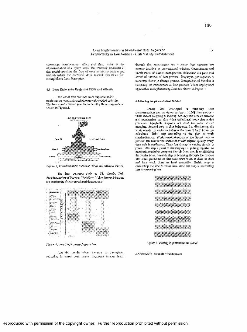
180
Lem Models and their Impel m 13PraJaaMtf In Low Veimne - High Variety Eeviraamettt
m inim josjs improvement efifcrt and Its®, (oaks at the Wipl«fl*ntffti«t at a at wo level. The i»Kia*|i -presented in this m otel qweifia* itte Sew o f steps seeded t» ia sa t i and Insti&itiwii® ill* continual A w e toaw d w w B ease flat sx«opts&* » Loan Kstterpsise.
4J Lews Enterprise I t e P at PSNS sad AUm tk
through tins experiments are - many (can ooaeepte aresowSr-iafetttir® to seBreiiiiarVl wisdom Csnsmitmem sm l wvohfeimet c f a e a k r management fM m m k m ibe j»oe awd extent •' ..&.■»>; o£ lean process. Employee partkipanm is s * » \ li ,roses*. sbtoogatlkra o f Iwi'sefks. sm em .t} u ti-i'nr,"’ , f lean process. Three deployment approaches i i i ' i >* >e * x Lean wo shown in Figure 4.
Ibo se t of k m methods wwe taiplaiwtlsd to inioiraize the cost and maximize the value added activities. The lean ma»fora>«ttion plan fowwisSed by those ohipywA » shown in Figure 3.
UNRlfeWfcRttHMtftfe
♦
TTgure-3, TtmKfcrmation Model at PSNS and Atlantic Marine
The lean concepts such ss S3, visuals, P ui, Slandardimskto o f Process, W «kftow, Value Stream Mapping ate used in the ahsavt-iaeaionsd depaitnisote.
44 Boeing iBtpfewsatatMW Model
Boeing has J” tW f " ii* 1 m.implementation pJan as r<j (1 * * 1 1 3 - J i f *,i » <» value stream M ap p in g ! * i h J*, f i n «„ taland information but al » r t to, » art it* - U fc tiledprocesses. Spaghetti dwgtanis are mod for v e t o stesromapping. Second step is line belaneu® ie . dBtribtsksg the work evenly. In order to baSartee tt» laws TAKT limes are calculated Third step according to the plan » wcrkstaiidaidiitcrn Week siandandiz&ttaa » the fastest way to perform tits to»c at the lowest cost wilts higbest quality evety time task it performed. Then fourth step is putth® vssuak in place, Fifth utcp h point o f w e staging Le putting together all materials needed to complete the job. Nest step is wtaWkMng the feeder lines. Seventh step is breaking through the process into small processus so that maximum vw A is done in isbop and less work done in find assembly. Eighth step is coovertii® the line to pulse line. And last step is converts!® line to a moving Hue
w m m m m t i :%m i ttiisiisH* B ill SiBSBIlii
Figure-4, t-ean Deployment Approaches !■'?gw«-S, liteeiif; ItapkmertatioB Model
And the testite show increase tn thwughput raductkm ia bevel osmt, waste. ImpcBtml lessnw learnt
4.S Mailel In Alreraft Slateteatme*
Reproduced with permission of the copyright owner. Further reproduction prohibited without permission.

181
Ale* K. Verma Anand Ghadmode Harsh Hirkanasvrar 14
At EL AL, Lean maintenance Is a business strategy to Increase tie profits that requires tactics, careful planning. sad eammitmea by executive management It requires long-term commitment and employee participation. The primary lean maintenance tools used by 0 A! included- Value Stream Mapping, Accelerated Improvement Workshops, SS.etc [tSj. Lean maintenance model adopted by EL A! Airline is shown in Figure 6.
workplace organization and ends with lean suppliers aid customers.
- t — -4 — — r
I w S
Figure-7, Lean Management Philosophy at Toddyfy.
* K«W «\V
Figure-6, Lean Implementation Model at El Al
4.6 Lean Rqaalr at Todd Padflc Shipyard
Todd is primarily 8 ship repair yard but a limited numbers o f new sh|?s are also built Lean implementation in Todd [19]is aimed at reducing waste, sustaining gains, continuous improvement, .and increasing profits while decreasing investment With help o f NSRP they developed and implemented lean implementation plan for ship repair. Lessons leant during this prcgect include;
The People are the key.Must learn from all we do.Standardized Systems & Process Focus,Performance MeasurementCreate greater opportunities for and through people.Wins for all.
Todd discovered that it's not kanban, ce lt w -S but tty people who are key in fee implementation of lean. They also discovered feat teaming on the job was a key component of Lean implementation, namely use of Dealing* s plan, do, cheek, act (PDCA), At Todd, the Lean management philosophy is based upon a five-step process on the Operations side along with an enterprise management strategy, co the corporate side as illustrated in Figure 7, It starts with
5. IMPACT OF LEAN IMFLEMEHTATIONS
At Boeing, lean implementation resulted in 50% increase in volume o f fli$ lt deck panel. 99.5% tines product was delivered on time and also quality acceptance was 99.0%. TOP airplane per month were reduced from 29 (before implementation o f lean) to 14. For 757 program lead time was reduced by m m f a n 40% Moving flow tine was implemented in the production o f 737 / 757 stowage beans. Benefits from this are - 23% reduction in hrs/part, 20% reduction in asaembty stations, 1500 gq. feet reduction in floor space, and 66% reduction in woA in process. Also predictability o f output was increased and all line stoppages were logged and i f possible fixed.
Lean improvements in fabrication division are - distance traveled by people reduced from 12,200 ft to 2,500 ft, distance traveled by product reduced from 5300 ft to WOOft, product moves and flow days reduced from 21 and 75 to <# and 18 respectively. Lean improvements to propulsion division are - 66 % reduction to inventory sad 66% reduction m unit time flow.
I&ju't- o f lean repair initiatives at Atlantic M aine are; ore ncxease in Throu^sput per ’W orte Rate in the Porttau. Fabncation Model Line, :33% of space available to eaablv iroic continuous flow and additional area for vslue-atole - sot c jdded work, reduced travel cost, subsequent time sitto.e ha> e “indicated" that travel cost is reduced by 25-31% a e o fee workplace organization efforts.
Lean achievements -in terms of dollars at Ei A! are - $ 2,55,000 worth reduction in w w k hours, $86600 worth
Reproduced with permission of the copyright owner. Further reproduction prohibited without permission.

182
Lean l t f s f t e i» « t* t l« i M edsb. and S ie ir Im pact « 15In .Law V olatile - H igh V ariety iB 'flrerttB tat
irrvetttofy redusstkat and pwebssing avotdujca, S 8360 vrorfo aha- saviBgs, $10,0W worth week area improvements,
& A GEMMLAUZHJ MODEL M IS M A S » fH JJM *S T A T M W
Thepropose s.* ” i Ji rap / ' n maintenanceiaeorporafos « sss« j , * -sree Wsffltingand Lean and St* S’gr irr >*-r\.r»>t o i ' M s ujos> toemodel f<\ new ship <r*mi j» • ke. rto Lamb (2f>rt>)a « as. tmiiatet beat i*i Loss . *<nd it <*. Japanese shsp- Ftjvi’ nitaity.
The foundation for wotid-ciass l o t repair and nuuatenant# staft* with process stA flizsfa i, which includesLean tools like 5S, sta,ad<trdiaiisoft, TPM and Six Sigma tools for process control.
The second foundation element o f the mode! relies upon value stream focus. Smooth flow o f material and parts through the repair value stream and iategratfoo o f foe suppliers aw*®* tirady delivery of product to the customer.
The ttsirt foundation eioncat u t te philosophy o f cwfonufMs improvement. Any worker can make a suggestion to any manager at m y time and it is followed through Continuous improvement also involves revaluation of processes and procedures « regular intervals. Continuous improvement keeps an orgimiKOwti eonspeitttve. The proposed model is illustrated in Figure 8.
I l k
■
.SWJSytfm.
Figure-A, Generalized impltsmoiiaiujn Model
?. CONCLUSIONS
The Lean mgiksrtusuatton model presented h*reassimilates- best practises found in industry today, 'ft® model builds upon a foundation of steble processes, valae stream focus and 4 philosophy of continuous improvement. It isawported by jtst-m-tsfss and buiit-ifvquaSy principles.
EBIHiESCES
f i j C.imwr>fS « n ,‘ L«to MjruLmturaig for foe Small Shop”, , wjet* J \<*saf ctirii.; ‘•ng'tv.'crs. 2001
[-■ ;anJtr'<, hrtkt, f t Ktjcecr fob, “Lean Repair Case "EnP a c V o i i foieR MSI5P ASE Lean
fwpbtuthng ft ,-ihip kto»sr p w im # 2 April 1*3, 2063 Sestfle, TV A.
[3] [3] Executive Review, "'frmsitioning to Lean Enterprise; A Guide fer Leaders - Votame-r, Massachusetts Institute ofTechnology. :20»'
f4j Feld William, Lean Mafiitftictising, Tools. Techniques, and How to Use Them”, The St. Lucie Prats, 2Wi
[5] Fxostaiscsn, bWs, “Lean Applied to Ajrmft Repair”, Lean Shipbuilding and Ship Repair Forum ■ 2 April 1-3, M , ffofo.’ s. WA
(6] Larson Sufan. lts'-aLtn$& Craig, Xlse Boeing Company, ‘ Me,. fo>fl w>vst'- iBuj es» Success Lean 'Matmenawe”,
l z m fhijH ui'dog . *<J Ship Repair Forum "2, April 1-3, "w? Seattle \Xt\
(7J Lejv At -space foitttftw Annual Repost, “Lean Aircraft ira lew c 'Mailed Assessment of the .Defense Aircraft M u sh y”. 1997-91!
|S] “Lem Repair at Japanese Shipyards”, Observations tram the Learn Enterprise Project Study Mission to Japan Lem Shipbuilding anti Ship Repair Forum # 2, April 1*3,2003, Seattle, W A
[5>j tiker, Jeffrey, “Besoming Lean”, ftoductsvity Press, Puhrtfaty 1998.
f t - I « i ¥ , !. i 'ib , T liot" iy <wd Ini-fcswjit aa1*1. 'iimsfaedjfEi Vedr' ft a r S Cirar.Ti.w!
kI\< ' »w»! 'tfn Cewsrw tKr” Mrntcob Ar.t »*,,>, faneft. 2 V
| , Nt f t ' . V,i si f t p\ «L jKi'i’i w ,i i ! ( neipka11,,-Hph tut it >;>v rj'stw I srng ' be ’ to rnsiness 't 'fttt „i<n, St tit ,4vg and S ’lp t n m 2, toffii ! 5 T*|A -’w a ttle Art..
t l ] f ti* jfof. j s '• ,he IrSemationa! Lean Manufacturing { 13J t^vnfereoce', Le3uagt<wi, KY, May 2002 f 14] “Proceedings o f foe Lean Shipbuildir® & Ship Repair
f ' ■-aegtm KY, -tats* 2002.[ ISj Seh- n > crgR irih ard , “ World Class Mansafactttring:
'P : \ i .{ M5«de”.. Free Press, May 19S6,
Reproduced with permission of the copyright owner. Further reproduction prohibited without permission.

Alok I t Verma Amtod Glmdsiode fitirsfc H tr itu a ta ir
! ( « • , >( - < ; i ' » , i | jrs > ' i r ’ i s< » <,>Ji ' \ t V? ni 1 Cad 1 ‘ i * ’ t*i
| l V„ ’ I t n S ' 1 i#>«r«v > f r j <» f*v K * , » i 1„ 1^1'’ ( 1 or > “H V S V »I A-** £i ‘1 , ' i TJ8 3 ' / , f u.-t, iu,i -> ,vn ’ Si-n>! \
G t «ujmu i «s< -sli . s >t, ~ ■> i v * & y? u fe jmm<y i*A>6
; 'y ] 'T’vf(isx*. 'an u»d J a m , IXssv* “ ibe Maeitme That Changed w World”, Harp*- A*p;wd New York, NY, 1991
[203.L*%, &iek, “Status of I * j | b n tv r<«* ftojescf" Todd IPseiEs, J'orum it V-1’ IA ’< “w iL*,WA.
}'21jB*fe«, I Dua ‘I 'I t tc I ng '"A tean St«y.”F(*um # 2, April t ’ </A Vrfjik Y A
Reproduced with permission of the copyright owner. Further reproduction prohibited without permission.

184
HAM I n t e n t « n • a * n : n i ; f l4 4 u ■ ;> <■
A Comparison of Stochastic toventory Models (Base Sioefe, awl (Q, r» In Two-TierSupply Chain
A S A '$£, V c n u u & A n te ! S . S ® a |e OldDcmtmm (•nfmiity
A tvfeif l'ii-gm-3
AMracfc We investigate ■» >te * i<-' t < t i a w /' 6 r A «? > >> » 1 <> * ’ •* i $ <, t r i i ’ s . i 71 c< ” ftokHngeortsaredsirgeda ' v ta*» a a i jsmsx <' f k, ur c n r< ovcrdu tniO' ' ; o i r op,?- |secondary supplier. Thispm . <>e » t <> <j i w u * - ot A e 'tot* tw in *t’tv «>- v j s U W ' - n , . sv.p- •> t i n « -implementing Base Slock tnyentory Mpflsi at primary supplier ana secondary suppiwr. the cusiaiser»oesB®id touows roissan distribution. Then we anpksmert (Q, r) model for inventory control at befc suppliers. Different cases are run by changing the repknistewrt lead-time and calculating the reorder point safety stock at primary supplier, secondary sajspher and warehouse for each ease. We calculate the inventory holding cost for both Base Stock Model and (Q, r) Model and discti® the results,
Keywords: Bullwhip effect, Stochastic inventory models. Base Stock Mod#!, (Q, r) Model, Two-tier supply chain, Fill rate
tlNTKOMJCTIOS
For a mmixc o f reasons, many ftnns purchase parts from more than, one supplto he our pi tiers o f order up to the customer depends upon en <n m i \ e y of parts from the sappier, tefeatoiy tnaaagetrcu the suppfy chain,is critical when the ctemaad is not detenu inktie. Demand variability increases as one moves up the supply chain away few seeondtuy safffes and small charges « ci«tem « demand can result in huge variation in orders upstream. This phenomenon is known as Bnilwhsp affect Thais, it is necessary to study inventory models for uncertain demand.
We have considered N ew s Vendor model. Base Stock model and X} A\U \<rv*.V *V rr -sk* m a te m
«*t in «•.*» sted with reality there is always some cost
son of an order. Therefore, v s ate
assumption £ha th r -prcduciasi aa or jar f > associated wife A 'Jura vOrt,i4‘r r ; F r * Stotlr i* n i r i As « J««i h i i- r per. Cv. t v>ir'r - oph 1 ids '« t~ v
b- tw ' j «*te prm n
# 'lOs n i J V * v I 1 O
{if o
«f S«ppis for two-
Poksrn
We have considered foe virtual company sreis a two-tier s«pplj" dawj. In first scenario we seStock favaisory Model at prim sy sappiief, sacon l«and at wwS»u«. We eafcelsted foe fill rate, pp satthe o fik s has strived before demand for eaw r » nd calculated wordsr point at Primary Supplier, Seermdaiy Supplier and Wtsrefeotse for five rep tesita ea t lead time fl 2,8,6,4 assi 2 in <mfo*XTaWe no 2)
SimMSy. we tan different cases for ( J r) b m k I -atd catelated the order quanlity (Q) and. reader p"tnt <j at tjntiar-' supplier', secondaiy supplier asd wm»howke t Fsb'e 5a •srd % } We have calculated customer sendee level and rjreter 11 friquenoy for each cage.
% MT3ERATOREKEVTEW
Wflson (1934)0, 2] has dsns major worSt on sStKtstionJ inodding of produotksn and iwentory control Wflscei teaks the snren&uy confrol prob!«s inio two disliBsd parts: !. 'Detenstiamg foe order quantity, which is the amount ofinvffiniory that will be produced with each m p k tiM m a r i. 2. Defcrmiiwsg foe reorfor point or foe invertsw t ‘ w * rt’ch repfeaistesfti will At triggered Y«-Sh«ns vr)_ f <* '2.3J s* J m l the . "Ct ic o ' i n, , t , ,i —r j s ,> - i e ! r , s Ik
r ’ •* 1 < -ttrj „•» L' 0 tit W * 4 i » ten iss / 1)r j i I t I Or .t d * r « v > i l iv k it ' i ;W » I V ’ (m L-tse < i 'A , ~w ,» ii s \ ! ) cldr ft \ t iS iL to ,sv»
i ’ y N ZW y, i4 r ft< ( ,!« " S ;- t 'ite <i ’r ( i, 1, tr •',.■! t;.,
r rttou ot « >r te a*i«.s v . / <. j r'pg ”>«* Jen, < thit * 1 \ i. i i sr»-i'uSr 11 5 n-v.
We Iwvc foscossBd tmother mode! i s . (Q, r) mode! where itw M sty i* morttotad con fem tsly and dmmmb o em ’•uk */•>» Sufcrsts?A te, A.K. Omtteqee f4] have rpptied(Q, i ,*■ • or e-mrttisage kwentaty .systaas and a!^»E«tk« o f
< rfA®, r iwview ( i , Q) m odel Am % % Jmg Lau m l i ' !« i % Lett P I presented vecy * ,irocedute for
e i, i - g foe optimal tot « .» atx. < ' xm i for foe
Volume 7.' > > C ' - *4©20041 r {.'
Reproduced with permission of the copyright owner. Further reproduction prohibited without permission.
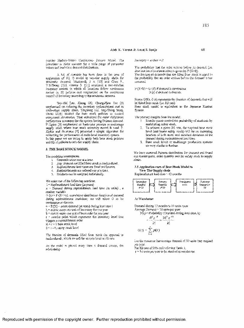
Alok 'K. Verma Sc kmol S. Senje '68
popular I- 3 s 'ith « H> - triew M odel Theprocedure ibl' B. Wid? snge o f p e w » « rvalues and »<• <f fn-> ’ >r no c
' * < .it 'W » < .Son J ** t<V ofV i - t o . •. ‘J t i ) w3-mt o prh i*'a far»>v n- cu »* < v. t* * j Jin r i r .
t * u , ' ' , > < > i c m ' i « tv • n . ' - s ncs!n " t o 4 ' T> -* V 'K * ’ l * k > v "OH , , ' t « r ' J t V '^ i K ' t <*, u ° jt‘ > vs ,r,J * ij r ii.< u ir < t*Ou.Ai'4 o» S i! w in n > „-ru~K> h u ' W . i * , tone *
Wefrkfe ] ,«n, Jihong 01', Chung-?isw T‘e» [5| emphasised on seducing the imetKMy tophausfament eost iti m*t -‘*i nmpt cham Yingttonsj U.', M g ** ig Mqg,Dotk» I ' M 'hw m ! >he b« » ■*tor*' por~to* "H I t, jp» j > _r* » »" I,* ! ftc r cmcal.*to Are 'Wi,r " foi i i
" • t j f * o f B f i F 's & f , , u*" i tr- M anph.M/n ir Hwini.Vr s -ins. •"» , » !!i t»«\*
jik ij- i •wM i ease f l r i - tir/cntov"' model » used. P. ' p i i 4 . id '> ' ' . n '« 4« [ 9 j p t v ^ m n x i a s im p le e lg o rs ih ff l fbar
esfaaaHng the perronoance of nmftt-kwel inventory system, to this paper w e aw toying to appfe? bdh base stock pcictes and (Q, r) policies to two-tier supply chain.
3. H I .BASE STOCK MODEL
The modeling assumptions:t . D onalds occur one at a time.2. M y demand not filled from stock is backordered.3. Reploiijli»ent lead, lanes are fixed and known.4. lU fdesfrtacnts m ordered one at. a tint*.5. Product* can be analyzed individually.
We make use of the following nomtksis .I “ Repknistoest lead time (in yaas)
x - Demand Airing replesiisianent le«4 time (m uate) , ai - SO. ti Vbfl O i'(.V C y ' -rw’iU " um ! Jtkm function of demand
toinrg ^plenw < ti .wd li < *e will alow <3 t» heorataC jt bv n* *
- r ['s ’ <s«n iJii am’ nj i ’ ty ^ iim« 1fi u . - ' t i. *s» o s c u . *< f ir * • K d < e ' ‘ srb i-* k rn u a k-A U u rr Ki ne i» 3ri - a , i l"‘ h >• » &« at»v.uay level thatfi if ) ,i , fdr
r i i>ay > M i*. -( \ • > « i ,T t e , h « > i C " o i < f c r i 'n d » if f ro m s t o r * ic - . o p i t j e « t o
tesku&r>4i, th <i w tin ssfvs.cc f e e t , < r»*’
As the order » placed ev-eiy time * demand cccurti, the rdsiioiBihip
Irffmkufy + . j ? f c «■ li
i * o a h r < ' • * t v» 4 id ( is ,J S ! i* v f n o t f H I y i v ,r P i ’’rt a- a « s r v t i n * t - J n J i toijt. i-’s.. « ...u.‘j jt .i.e ,. o-.j,..,, Lw 3 it t ooccurred
P (X<R) ” d (R) if tkmanil if c,->iti«k«s ■Q {r) j f d f ttB in c i r d i s c r e te
lienee G (S i O (i) Kptosenh the fraction o f .deatsnds ilia! sriB be filled from stock (3.e fid rbe)B « e stock m odd is e^cvslertt to the Japanese KanbanSystem.
The psinwsy isissglsts bem the model:1. Reorder points centos! the jmobabi% o f stodcouts by
eslabfiifetr safetjf utodc.2 To achieve a .given SO rate, ifog required ta se stock
level (sad hasee s d m stock) will be an «cr«ssing flmcticm of both mean and stemkrcl deviation of the cleat and during reptej).shsn«nt M time.
3.. Base stock levels in sndiistoge production systems are very similar to kanisBt.
We have asswned Pofeson duiributkm for donand and found out isordar point, order quantity and the safety stock in supplychain.
3.1 Application run* o f Bw e Stock Mode! to Two- Tier Supply *f»in
RsplttriskBfflit lead time “ 12 months
j SwwKtey SapjHiw
F*2S
AtWrnndMHoeDemand dar v w *4^* ’P jncis/yearAverage * w itrr-\y , vaar
ftk ) = -/ <b h*.«, 2 , ‘ ;iA a iag .tead tirae ,k )
£ c f !'M 1sa ------- --------/.: k.
0 ( f ) * S p C*)%*Qsomsr lm m&@g$ ihmmd o f 10 umfe (say
psri <rf 9054 ati,d refesting Ttbfe I,
,. wxoiperyeartobc stosW st w^kjuss.
franwy&5PK«
r»i 9
Reproduced with permission of the copyright owner. Further reproduction prohibited without permission.
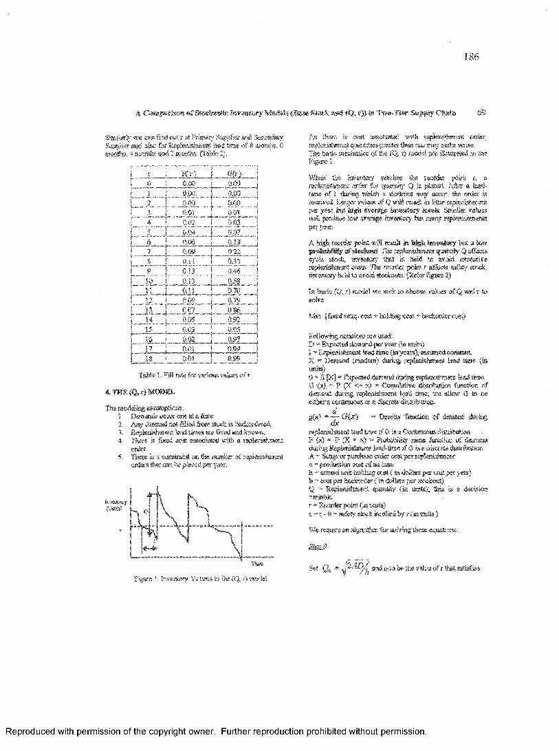
186
A Campari son or Stactasftc Inventory Mcwleis (B u t Stock awl (Q» r)> in Tw«-TI#r Supply Chain 69
i w >r,' *r* c « u> -•« ! i" 7 ot ppi r^atl Settendary'As^a’i -no tK» %«:„ t «*!, § months, 6iitf-'J’- m .' Ya / t w ., ,;•
F{ f j mi.0.000.00siCO ,1 At AiV ■
.0,04.0.060-09
a. a■~t
0.00 \o.O0 .0,00
J).£L0,036.070.13
i 1 0 0.13 i 0.58 1
r n .... 0.11 0,70 ___jI 12 0 .® it ^ 1
i 13. 0 0 7 0 do 1; 1 4 ! )(’< 092 ~11 t s _ _ ln& 0)95 1\ 16 0.02 0.9? 1r 1 7 0 .0 1 0.99 ~11 IS 0.01 0.S9 i
Table I. Ml rate for various values of r
4 THE (Qs r) MOMEL
The modeling assumptions;1. Demands war* one' at a time'2. Any demand net filled &<*» stock is bac&ordeted3. Repieniafancnt lead times are fixed and known.4. There is fused cos!; associated with a replenishment
order,5. there is a constraint on.the lumber of rqjJaiishment
orders te l can be placed par year.
"'n Q
v ’< /» * c/> ' U at* n 1 *ep) t«V*> ttt, t.f» * ■ h.*, , i w t> i n-'ter^Kr, ,t r v ” r>’H ' wAir w • 1 ' v * >r«;;«
sr,
. t.<As
o f t s * v r « n h th e > x , > . i a
v r « '» •»no' or ei i. ;ua «» v " o c- ,*)« a 5s.«d~t w <f tlaMs mAi votAtit*' rw* o»,% rhe , o ' is
w n d ’» '* v 'txse 3 -.il (w! >i tgn r.nt-i,* cat f t tfM t*_' s'isfk m s m ^ L « » »la. / t t e h v „us$v *f ja-’-i v »> r f j-e i ' f. ry N r m w t j't! its
\ S«iF.
a high i murder j» k t will resiul. ir hfeSi SnveWwrv but a low probability »r *4«e&.wt „k*i«pl,F'«sfei4* s ij_ w t v « A t e t 1. r>v,e .s' sfe •*» A tor* it ! tj 'v 9i * t e \ i s sonjfmwfraarttt »v-’i£ riw s'jrtkr pos* r A -t. .ociimmtmy facio to av\»d t e m U . (Ketar tigtsre. 2j
In. ’bask; (Q, r) model we seek, to shoos® values o f Q and r to solve
Mta (Iked setup cost + holding cos + becfaxder «wt)
Fotlowing notations are used;D » Expected tiatatmd per year (in units)I •»■ RepleBishmtut lead time (k years), assumed constmt- X = DsaiftixS (m tas) duricg Kpteaishment lead te e (in units)i A p v j P x p e c t c J d c i r v i d <£s- n g f t p l e n i s h m e n t l e a d t im e
F (X ' * in* Hr-tt roi riot f u n c t io n of tiwnrfia jun ig rap (b -t iw !<nd ► me vs* iilow G to be
9 M. posuou* r* a «.sei«* <l»tnbiten>
Dsasity t e e t e i o f demand during
i^pfenshmcai. lead tec *» ex Coctmuwis d iu te tea ? (M - t (X “ 30 “ T\t,twoil iy mass femctiai o f deosaao i'w;nv Ri'pletushassn!: ksx %imo if S is a discrete disfejwtet. A Setup or purchase order cost per replaislsaeai o - protiucfion cost- of m &<m h. - anawtl unit M !dm^ cssti m dol’lass pa 'unit pet year) b ■ s»st|wr tackordcr >. ;n '*.>lfi-TS per stockout)Q - Kqdanisteienl ^utinuiy fin Brats); this is s dem km vsratblc-r =.Reorder point (at units)s “ r - 6 *■ safety stock implied by r (in units )
We require an algorithm for ariv ing these equations:
afffj
®C! 06F%«k i. Inventory Vs time in the (Q» r) mtxiet
s |£4i57 t /.» ssisl a io be the vahie o f r t a t satisfies
Reproduced with permission of the copyright owner. Further reproduction prohibited without permission.
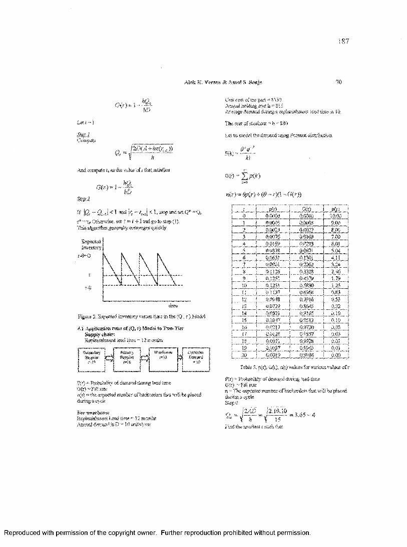
187
Alok K. Verm* & Am d S. Sonje. 70
0 ( r ) -
.Lei i - 1
ismiComputellD(A+h
And compute r» as t!» value o f r that satisfies
(3(f) l~ ^ L
m ihD
tt f2 t~ Q z J ,< l 9Btik ~ f M |< l , s t q ? and set <?**--<&
r* «T|, Othsrwise, set f = t +1 asd go to step (I).This algorithm generally CMwerges quickly.
Figs.®! 2. Inspected ijwantory va rsus tarn® in the (Q» r) Model
4.1 Applieafisn ram of (Q, f) Model to Twa-llsr Supgriy stats;Eepfcawtomt lead trrae •' 12 .month?t
j ScondnySappliw
I j*J9
BriaatjSsppSsr
sw!Sr--I3
? t - f lability o f demand daring lead time Irate®5 *cted number of backorders that will be pissed
, y a k
fa r wawboaseReplenishment Lead K "t 2 r.r-tA.;Annus! dets»d is D*' 12 >*nisW
Unsteosf os tne pert «* I >50<• ’i t f »1’ t * >• r i i r , jtfa ta s lam tim e» 1 0 .
The cost of sttockout * b ~ I #
Let «s model the demand usksg P sm m distribution.
0 V *m -
M
< * » - £ * » < * )
«(r)-^(r) + (tf-rXl-G(0)
_ EsS 0 .0000”
0.0005
.JL910
0.0023J?ZC*LT r i v L
COT11 Mu »:0
251
l.im.
.SO* *',>■}
OOlifi! } q u j> o 7 i
. V ’_02V2 "0 ’378
O-ST*
u 9*530 '
nCrtL o k f
9.00TaT7.000,015.04
. .M L1 .2 4
2,461.79
131415~
J L
"20”
/, > > 9 /■ • J ...0.?3_,Ok 4tj_ r
f _7>,4i 1 0.32j _ <* luA i 0.19
0 u*~ _ ~ r—i- Of- B i 0.100,9730 j 0.05
"o.om ~ c - v * 0.03i» V 'j It':1?!.,,.u
T__0.9£oS__ j ....M i l ,
0 0 ■? i 0.80
Tabfc 3. |.<r), Q(r), aft) values for various mlwss of r
Pfx) «- Probability of demand during M i timeOfr) Fill ratea Tie expected number of backcrdasB feat will, be pieced during a cycleStep 0
O h a d 12.10.10! h 1 15
..Find the smallest .r such that,
= 3.63 - 4
Reproduced with permission of the copyright owner. Further reproduction prohibited without permission.
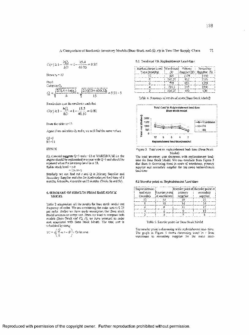
188
A Cowpsrisea of Si«fcsstte Inventory Models (B»se Stock and <Q, r)) I* Two-Tier Sappiy Chain 71
G(rt > 1 - = 1 - -221, * o.S5M> 49,10
Uenee % * 15
Step!Catapult Qi _____
„ \m A * W h ). ck _-,----------- ,-- 5. j | . 3
Recalculate tj iw'i i sit that
G (r)£I~ ”; *1 1 =0.81s' -KJ. >M
Fro,® fee aifeie ft-13
Again if we calculate Qj and rs we will find the same values.
Q l-5R !“ 13
\ep. ■ 4' p.i. . iu ", t 1 ’iPi. >v*sKrd i)
moaty wxlar?($} t r v .925 5 H75 ! V
^ 0 5 " ' r *
725.5 I 1 7 Ma n u s ’" 4 V f ? J S f
Istfek 4. SianBisy o f m o te o f awtsfBsse.Stock M xfeS
33® ,
tenlftw
» - fVWnusat?, « |
SS
8 8 4 2R®pl«S$lwtt ts*Jttai®(n»ar»iM)
HENCE
(Q. r) model suggests Q“5 and r “13 at WAREHOUSE i.c. the engine should be replenished in a yw wffli Q**5 and should bo replaced when, the inventory level is at 13,Safety stock level “ r-O
= 13-10=3Similarly we can find out r and Q si Primary Supplier trod Secondly St^?pli« and also for Eepleaisteient lead, time of 6 months, 6 months. 4 marts and 2 months (Table 5a and 5b).
S. SUMMARY O F IB B IB FROM BASE STOCK MODEL
Table 2 sununsrims all the results for t e c stock model sad freouencv of order, Wo are eonskteraig the order crwt -if $ 25 t* r r ; j f|irw )! ’ nii<te wswnptwi t ’ r -*'» stock
"i < #t Since we- warn, j U’r>- sk both u i 3 ' we have assumed an order
k«v 4 jck Model. The total cost. »
r >t i . mi- » o f ^c.rt S«. iFR ’t ku •>* a' i »«nffol U ! v
2.4, r2 i
rC « cj ■ Order coa.
Figure 3. T< replenishment lead- time (Base StockModel)
The total jm w t« y cost decreases with replenishment lead- time for Base Stock .Model. We can conclude from Figure 3 that there is decreasing (tend in costs of warehouse!, pranwy supplier and secondary auppfer for the sms- lepteushssemtad-ibm
5 3 Keontar petal vs. g q iw is lw w it t e d thee
M xplm M m en i > ptaxdarpoint afReorder pda* atfort time » eorrtr p'"rtj primary j scewtdaiy{meads} »• t4.-eh.viw; | asjiplfcr j sugpiter^ .
! i o | 14 i ~TI>1 I !j . . ,
1.1 "+-• 15
Table 5. Kmdtsr pomt for Base Slock .Model
The reorder posit, is decreasing with replenssametii lead- time. The graph in Figure 4 shews decreasing trend in 1 from warehouse to seconttary supplier for the same i<*a~
Reproduced with permission of the copyright owner. Further reproduction prohibited without permission.
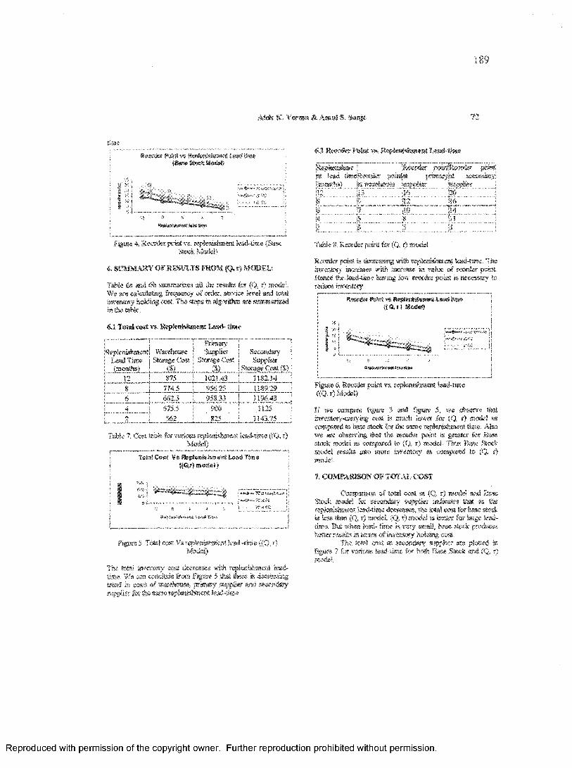
189
Atok K, Verm* & A«eS S. Semp
timedetmsj “obit A«pienis!ur*nt»cab liw
*f5a«tS%re.,&iwMS
Vi
Figure 4. Reorder point vs. replenishment lead-time (Base Stock Model)
6. SUM M ARY OFRESULTS FROM (Q, r) MODEL:
Table (m an d 6b summarizes all She results for (Q, r) model We are calculating frequency of order, service level and total inventory bolding cost. The .steps in algorithm a« summarized in the table
6.1 Total cost vs. RepSemshmcnt .Lead- time
Kepicrushmentj 1 3- c
Lead Time j S t o a t Cast: (months) | fo
12 | 8 ft8 ! 77*-«
1 6 ! 662 •»
Rrmaty jSupplier j Secondary
tarage Cost | Supplier(8) j Storage Cost (S)
1021.43 | 1182,14956,35 958.33
r ~ I I 8 9 .2 9
! ” 1196.4367 > ■> 5 818
_1143.75
Table 7. Cost tebfc for various replrasislsraara. lead-tsroe ((Q , i )Model)
i Total Cost ¥ t fteptantefwent taad Tim®I {(G lraeile!)
<i2 Reorder fe in t v% Reptadsfeaent i« ssM i* »
IfepiiisA iae j f fo M rd e r j x & i p t e a n t e t p c i i |lead timoptamfer jwiafa. jsmiarypi: secondary
fitnoriihs} warehouse teag4i«r kegrtier j* iB 116*"" i > ......................t
" § ..................112 .......... J<5 f^ ^ . .
'Is.......................§~ i l l" ......................i
Table 8- Reorder point for (Q„ r) model
Reorder point is dssreasing wife tepJe-rwtmeat tad-time. The inventory increases with increase m vafas o f reorder point Hence the- tad-time having tew reorder point is necessary to reduce inventory.
tteorder Mrt vs ttegtertslwawit lead ftn* jit«, r) Modus) |
I * J| V i
Figure 4 Reorder point vs. replenishment lead-time ((Q, r) Model)
If we compere figure 3 and figure 5, we observe that mventaay-eanying cost is much lower for (Q, r) model sis compared to bass stock for 'the same repfcwshmeot time, Abo we are observing that the reorder point is greater for Base stock model as compared to (Q, r) model. Thus Base Stock model result* into snore im tm xy m compared to (Q, r) mode!.
7. COMPARISON OF TOTAL COST
l«sss5>'95yi'3W-4*»t t'f.Si# ¥fj»d
Figure 5. Tote! cost Vs xepteairismeirt lead -time ({Q, r) Model)
The total inventory cost A.r\fiv«~ '•nth repl.‘’' c * w n t had-time. We cub. conclude from fog’.! r 5 <iV 'i’-.rr et i em&tfig trend in costs of warehouse w m ' wpiter ate secondary supplier ford» same repiwisfttts.it Isad-tiroe
Comparison o f total coal id (Q, r) model and Base Stock model for secondary supplier indicates that as the replenishment lead-time decreases, tlte Irta! cost for base stock is less than (Q, r) modeL (Q, r) model is better fo r large tend- time. But when lass- time » very small, base- seek produces better results« terms o f im raitny holding cost.
The total asst A s e e m k ty supplier are plotted in figure 7 for various lead-time for bofo Base Stock and (Q. t\ model.
Reproduced with permission of the copyright owner. Further reproduction prohibited without permission.

190
A Comparison of St«d»stte Inventory M « f* <8** Stock m i (€J, r» in Two-Tier Sapptj Outfit 73
TsSaS Gat ¥« Ketpfeirtstesat teasl S&mttxy SS«*?r j
! I 2X 0
I I r%7~I ,M> j a soc >i 1 0 4 -
-2>»f, ’ j;
12 » 4 2
IFigure 7, Comparison of total sost for Base
Stock and (Q ,r) Model.
8, Condusion
Base Stock w d (Q, r) iasrerstary control modek arc competed for diffiseni replenishment lead -ame. If we compute the results from Jafefe 2 (Base Stock Model), table da and fable 6b ((Q, r) model), there is significant decrease in the freqjuenty o f order in (Q, r) model as compared to Base Stock model The frequency o f ardor plays m impomm rote t e e , ® there is cost .associated wish placing 'the order. KeptesishniEat at higher frequency Iwwevor, m*y be beneficial firms fee point of customer satisfaction and Lean impleaseatatian.
Base Stock model em ptesias on replenishment qwartiiy o f I and it increases the frequency o f <wfar. (Q, r) mode! provides tower total cost,, since fee frequency o f order Is less. 'Die Service factor cfctwnsd for (Q, r) model is in the range o f 0.94-0.98, which M is within an wecptabk range for most ecg tw a iia m
Though t ’t itw-t ,eb-wd B^tiiBpUoo o f jo order cost for Base Stock model, we are creasing cjmror/r platform forcomparison of both o , o Yh.> tote1 cost fo> each cow is calculated The lots! coat include* the im'tnforj hoMa cost and order cost. T?stt, yfo si iw xkl it stifew r Vvos Br.sc Stock: Model is the two- ocr supply ehe n Ji*ictssed in this paper.
4 . i - i j t % t j ' , T u . i p t,ohctosv*t«k fwseduvl%'* {*%<! . « „c for fell i»0 rsig
, - 1 *-t . J to5. P.u ’M ’ r frvvnc , t taig-i cv 'V
ju IP'S* S'fiA o ‘‘ v *’»o n«>*.<-g T ' vJ f - »rsrp> « t ,r> _b- Lt .i -wcif-a 1it,-hi -J 1 v M M4 c" 2 to
6 . t rn m w y t ! g vwn>* r c c t ! Tact M-;,’, ,j|i r te i«<1 tn*v \ i i fo arsce
d&srtci A t * o i i' ,^«K Cte i., , i u i system"O’ci'dif'fl 'V tm j \t'i 1 >c "*
7. a ? j *jBg * n g Isa. titKV’himig Lsu, "A Suapk’ust f'pt:'<’t?3t,cn t r^-cdu-e for the (Q, r) irmsrstery
mcei bevclispsitnt ar/i svaluatiea* BE i r_rs ic i.o m 4 1
8. -> T*cktr. it "V| ‘C, i f 'r»< m i ooopafatwein enfo- m p,o-isc.ges s ifp iy -chain*- *s» ? 'trnoc ’.> 719? v *»3
9. S>o««v>«; >i, K 7 pkm l9 8 ■‘estimating the periamiance ot n»ultt-Wet Mwentory %'steas." Gpefatians Rasaarct; Vo< T 17-1%
10. MuefcstsA, 1. A. 19?/. --Analysis o f a two-echatan fw « tter / sysJem m wMeh all iositiow M towcomtimious review .fs,S) policies,T ectoisai Sejtort Ho. 337, School o f ClpsfstkMS iReseatoh wid Intfastrkl Bigiaeering. Cornell iJniveisitv, Ithwa, NY.
11. Gr«»es, S. 1996I"Aimjllied5efon a v e s ta y model w ih fixed repteniishmeRt In tarab .” Managesaeni Sci. 4.2 1-18.
1,2. Osan, F., Y. S. Zheng: 1994. Bvataafsig eahelen stock (R,aQ) p o lte te in serkl prodoc.ti«ifi®'eofo«y systems withstodiastic demand. Management Set. 40 1262-1275
13. FederGruen A sad Y.S, Shaug “A Siapfe ssdeflkienl a%arithm forcotnpoang optimal (r, Q)policies in iTontintwns E w iew Xwenteiy Sydsms “ Operatiofts reseanji.
!»«.' stw'* <t>o. %1 proves to fie teliet for s ia s l toad- time Ffc' to-s to’ti >"«■ {Q, :r) saodai ptoduces Sow inventory hedd t»g i? „t v > os, n .a Base Stock mode!.
K B H O G S A H ff
WifasMt, 811. 193 - , or® for StockC te te l Hsr iM c m ' o w** ’ V ’): 116 129WaBw -fop, t t • r S-x „sruj , “factotyPhysics 'n ii'Ytt-Sicw 9 rt>y Or o f slochatifeiiwanioiy systom. tf*t • vi * >*, 5Mt Sctotsce,Jaa 1992 v38 itl
Reproduced with permission of the copyright owner. Further reproduction prohibited without permission.
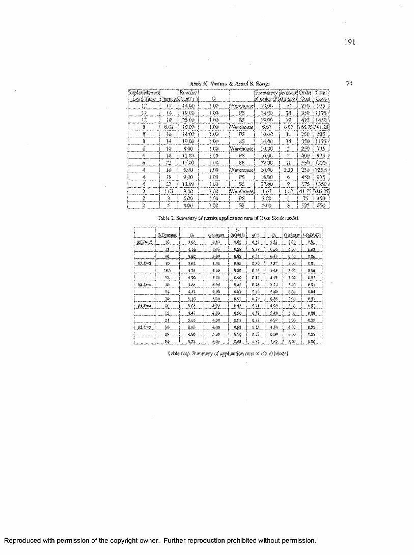
pk JiA\ A . k
Ak$k 1C V er«ta & Ampl S* S©i^g7 % ~ j ^
c n
j '* *
Ziit ft"?j y1
rJ . i ? i
»'> / 2 (V
-L’-'
« *;_________ _
6to j v ' !,. - s - j ~ ; - - *
6 22 1 ' «4 10 1 6.00 14 18 i 9.00 [
22>*,ii
s • i k)
tv?.oo_i.soLOO 1.00I M i
\ AitTV
J i t -i '\ r { /
IWar&hoaaei■L i s - 4SS irJ»v 4**4*
IS j i s w :
’Watehota,"p s "
4*- ■WV|, »e** ' 2 . I Tots!J V * Cost I- ■$*■
M j 350, %
[ I, I” r 4"* * « K
SSsWarefsswisd
14.00_’« C
iaoo
>.t>7 !66 .ir “>,»i2S
J -»«'325
• - 1 L ?<; v i i v*>•> ii i | . _ _ _
3.33 j f v r , 2 . 'PS 18.00 4 r l
L „ § s ._. 4.
V1 " a s "
] 27.W
1 <?i 5.00
i L
975 j3501
_ »(_■>>? _~_4vj_2* i ' ~ « ’
Table 3. S w n sesy of restate application runs o f Base Stock model
i- T"</ADe'ffiMMt , O'
J# I 3 AS
13 , <16-f-
o titfi a __j [ p« t'f! ! '<33_ | i 324.00 | ASS _! J.2S
•A C s '1 to ,O.fctl j 6.0U J r?
i$ 4.62 5.0O 0.8S 0.34 4A? 5.00i E i M ) to | 3.65 I 4.9C
p : ! 4.34f
V*® < AI k u x i to i &.mp — “ ] “ !4 ' Ir f 3# { 5;W i %m
Ell>1
4_ *>29| 0 ^ f\ h&
! a :
j . Lr
* op ! *u
5.3 5 4*
SS..91?
6w*f for
Sa’O
S t j
_f J/ISp*
«u
0-81
0&5 _ OS1
J 1* t .±I„f £}r «eCVf*
’Vss*f'
Table 6(a), Summary of application runs of (Q, f) Motto!
Reproduced with permission of the copyright owner. Further reproduction prohibited without permission.

192
I J A M International Journal of Agile Manufacturing
ASSESSMENT T O O L S F O R L E A N ENTERPRISE IMPLEMENTATION
Alok K. Verma Harsh S. HlrkanBawar
OM Dom im on Umvertity M>rfolk, Virginia 23529 rJSA
1. INTRODUCTION
Lean enterprise focuses cm the efficient operation o f the entire value chain, from supplier to internal processes to customers. It is therefore very important to assess the progress made during Lean implementation by periodic assessment of this effort using these tools.
An ideal assessment tool must capture performance within various facets o f Lean implementation. It should include assessment o f Value Stream Mapping, Supplier management, Takt time, flow, TPM, set-up, Poka-ycke, Kaizen, production plaining, pull, inventory, uptime measurement, equipment flexibility, employee training, quality awareness, standard w o t , etc.
Figure 1. A generalized team used for assessment
Lean assessment should utilize a team Figure 1shows the key personnel that should be involved during the assessment efforts. During assessment, it is very important to include people who are immediately affected by the inqjlementatien of effort like workers. The supervisors/Tearn leaders who overlook the process should also be included
along with management. Different assessment -questioners should be made for each group.
The fundamental goal o f the assessment effort is to add value for the corporation, and to establish better conmiumcation with the workforce and members of other organizations.
2. LEAN ASSESSMENT TOOLS - WHY?
Lean assessment enables a company to establish their progress mi the “Lean” implement alias journey. The Lean enterprise assessment has a set o f questions that explore progress in key areas. There are couple of questions for each area with multiple-choice answers. Many of the questions will require seme research. The user is required to evaluate the relative strategic inqjact of each area Implementing Lean practices involve changing a wok area or a business process to maximize efficiency, improve quality and safety, eliminate unnecessary motion and inventory, and save time. Although a company implements “Lean” principles, it is of no use if it is not Implemented completely. Here assessment tool helps in identifying the areas where more efforts are needed.
The basic requirements for any assessment tool is as follows:1. It should be simple, easy to use and require minimal
time to create instructions and mechanism for use.% It should focus on Lean attributes.3. Should be able to accommodate all levels and
functions o f an organization.4. It should provide guidance regards future course of
action.5. It should go hand in hand with company's goals.6. It should not give ambiguous results.7. It should have repeatability.
3. CURRENT LEAN ASSESSMENT TOOLS
Volume 7 issue 2 2004 © 2004 IJAM
Reproduced with permission of the copyright owner. Further reproduction prohibited without permission.

193
Atote.K, Verma Marsh & H irkaw iaw ar 32
3.1 lean.ASSESSMENT TOOL
This tool}"! | was developwd at university o f Toledo This lean tool is intern* j Ire a sereeuag tool, for estitbiifements feat watt t , &$•> * level o f * sn practices bang trsplew.entee is their xu»ts
JHs ‘f H «n * <*ual A »*u ,} ,>iyf )«■sin m u ter *. lit" fo te < j a® tic*, TV eniiv> ooen v H 'u lv . no ' ^ c a . r . o a r f a , Tn'’tc o j‘<: and m vrtosy U .i/s.sg p< 'T.*n>" n mtenan,..' and n w lfa to tsjah r gr& ter ’8id;.ra« m aig i t f a fat"! leannfa4'!»l ts-A i-e e She 'Wtfu! >s ai fa k>*m c* j excel
i i . 1 1 { , , j, lonrtj? tft,’ - *rccni%o „r ’ «?*> urptoirentas j ,i
Oswsn practices lave also beta included in the assessment to showcase how environment ■ ft'tea # c m m a will Wt> not just (he organization «tvc money hut will also contribute to poBation prevention.
j 2 v m o i x i v s m l w w t M M m fA c tm i’mEXTENSION P A R T N E M flP fV P M E P } LEAN ASSESSMENT TOOL
VPMESP [23 las developed a Lean assessment tool, which can be used to compare business enterprise against world-class metrics. This lean assessment tool has two purposes. First is to enable f a im - to tA * im m m y o f those Lasn best practices that are «x.r. c fa u ‘he entatprise and how prevalent those practices a»e fouri ('rmigbcut the business. Second is to provide the user h A •*, 'H.areness of those Lean best practices fas are so place or-are not ctmmtfy applied and haace, should be ooastdercd for tmptementetkst.
The Lean assessment tool cantatas ten category worksheets describiig fee Lean best practices that constitute fee following attributes o f Lean mamdacturtag.
1. C tm w i f U n & C >' «aSawareness2. \ i U 0 X workplace organization3. Ska If id 1 4.4. Co-a r> p "y^ ■*....nt3, Ox .{fa <6, K mw pc* mv, 3~A Yoke7. SV t T <2 i ss.'jjM'ni5. T J J 1 n i t oua '.iasteaance9. P 4 4r«,-10. Bataiieeoiiow
Each category waSefeeet needs to be completed as part o f a review o f the actual situation in the enterprise to a s s fee accuracy and sfffeaMlity o f the results. Final result# obtained are shown in table 1 a id are plotted m graph in figure 2.
3.3 A MODEL FOR EVAUIATING THE DEGREE OF LEANNESS OF MANOTACItlSING MKMS
A tm m b , fa w s e it t for m tm sm g fee degree of tarenea# possessed bv atarai&cturiog firm# is made [3]. Research guv*. * <.i> % "-I- ow. v'd t* <.,pasted into ateuctraed a»'n< ..jufatt-iawir'** rot t e n manufacturingiire< j-j t u i &inr^Tf, ‘ vx. ~ ms < y u4t>- w*
Jto«esw'i i <0 >> «r't. t fc o i , o i 1 or*ct»svc. or v asxyi • 'a. to «ei *' t*
VI e.«t ws iSltk-j- e f a sU/ jsv< s» refn.wnt* d t. 3>>'or*rKm<ve• > j t or o, me sta**- ol ■« * m d*a( w V
gu i t den’ 4 42*" od. *"<tr hi •» thtisss ws-jvt "nJ t q'jpntitm < r f ' t . h v ,>f V»onevs were
Tanti.4 it!<* nrnt n0n .A xs«<- »i_ \\i i.>*ilr»ri-. ut-vrvetre'iif J* a»' k i o c i u ’A ' } ’ r C ‘u \frte~ i.ITi i.t<f oi sitswtais (PuLL), raalirfuaoJienal teams fh* 1 y ifecsttfrshiaicis (DBG), integration of functions (IF), and vertical irforaststion sptoms (VIS). It also incorporate fee measurement o f mmagerM eomtnita.ent to lean prodocticm. Questionnaires were designed to measure variables related to assessment of adoption of l« a production principles. The questionnaire measure two dependent and nine kdepesrfeat virsabfa as follows. The first dependent variable, “degree of adoption of lean production ixsnciples" (1DOA), was rated on a seven ruint scale. The second dependent variable was “degree o f leanness’1’ (IXJL), was measure as a mesa of nine indepsadast vwahles defined earifcr. This paper argues fat, feo^t developed speetfkafty for f a tafefcwaw tnfeiary, The research instramantcan be atipted for use ta other industries.
J.4 ASSISSMEW TOOL BY SATURN’ ILECTROIfflCS & 'EMtSWISSIMGWC.
Hu# aaressmrett tool I4| was dsvrioped for sitppiiers to evaluate fair progress toward implementing a lean business system. The four categories (Oisarazaticwal esB/ironmetS, Systems, Tools ami. Teehis.qws, and Metrics) fcsia f l» :foundati.s>n &tc a holistts approadi. to s fan business system - a»8pprsaifefott'«QBBgssfe»entireoigeniKstioesk 4nt dr * * ;» rifattaate waste. The primary use far this t m u m * " 1 r <ix orgftttisstfon to sste ts fter progress toward sns'hT * y t # lean, business system arad to uncover ate® wb.iv astlvities treed » oca * to spur tatprovemcss.
Fotlowing are f a steps tetea, during wessment.
1. Select a representative ssuijple o f fee oigaiiizstioii (comprising all levels aad all tactio n s) to fill out fee Assessment A sample sire o f 2)4 to 10*4 based o» otganizsfen, size wowkt be appropriate.
2. Gather the completed .Assessment# and compile fee tesaiss.
Reproduced with permission of the copyright owner. Further reproduction prohibited without permission.
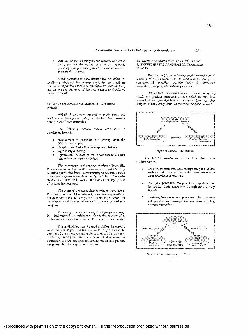
194
Assessment T«»!S for Less Enterprise Imptemeatation 33
Resuits can ^ I as « pertplawraig, an wgaBisition »< *«,
!) i/H ,1 rap* <i» f» usedn re» t> ‘twtegje
, s’ ■**«.* with the
C tt **• a. t* v a <» » in t» s t n ' 5 * ? *d, results Stte l’« •* *4 > 1 9 ' s <*. > w . l( » i rse manberof t* u» uto A ** 5 r - i 'nisslircs,asd an avenge tit*' each of the f tw categories s}»a!d be calculated as well.
3.5 WEST o r EJKJtAPQ) AISR«PACJE FOKUM (WEAF)
WEAF 15 developed this too! to enable Snail artd MedtaflMuat &a»tpr»es (SMB) to establish their progress during "Lewt” tfflplemefttathn.
Tlw foUwnig criteria where established in developing the tool:
• Involvement in assessing end scoring firm (heSME’s cwn people.
• Simple to is c Radar Scoring {explained below )• Agreed ta rg e t sconog• Qppratwrity for SMB to use « «]f-«j»ssm©is. too!
(dependent on Lean kuctwtadgc)
The assessment tool cowsttt of simple Excel file. The assessment 8 done in HT, Autonoiaaticn, and FMS. By selecting: appropriate b<«es coimponding to the tjuestions, a radar chart » generated tw shown in figure 3. From the Radar chart a clear visw can be seew of the maturity of fJejAmnail of Lean in that, company.
The canter of She Radar chart is zero, or wotst score. The outer most area o f the radar is 4, or m dose m possible to the goal yon have set for yourself. One might even use percentage to detemtine »!w« each exfioator i« within a company.
Far example, if visual itiaongement program a « d y 5W4 implemented, you might score flag indicator 2 out. of 4. Scale can be increased, to depict rastfe that are more accurate
Thi i f # i* St*,! I ! ! SB *, >sp«>sikareas that \ n., j- 1 t »«.»' rs j* 1 Vcamtaictssi n * d r 'k * r> t * < ' *. > syneeds to g a reog'itd »n i t s , ’ < i t jt ; i u»ss structure ’» -in* H. w i 1 *\r,.\ r>* *twifi give sustainable improvement is? Lean.
.3.(5 LEAN AEROSEACE INITIATIVE - LEANm r m m m w , s e l f a s s e s s m e n t t o o l <l a i -LESAT)
T!t» » «»>»•) Jy 1 i s' j , > mfea tam of aa ents. .w m, it i%/*>ncniplfce* of c a v 1 titty «, '?»*• « *leadership,lifecyrl\rnvC. v<*s ‘j j i ” .s.
SJtvtBteof • y i.
ii >1 < j
L-BSAT toolr into ccsuitkratioti ?hs entire enterprise, wMefe the |wvks» m m i m t t tool* Med to take Wo account It also saovided befit « m tn n of Lean and Qapsnaiysis. It a'ko ckariy iiajtifks 8» '"next” wtepa to be taken.
? ■ ■ 1 n’3 i*y4'Hmrffrt&A&'jr ■,
/ X
figure 4. LESAT Architsdw®
The LESAT architecture consisted of three mainsections usiwaly
!, Lean tr»wf«rwati«»/l,»a«lership: line process and leadership attributes nartenng the tratisfonimtirai to lean pnsieipies and practices
2. l i f e cycle pntcemea: fiw processes i-«pos»ible for the pnwtect from conoeption fiuot^h poet-de!iv«y support.
3. E aaW ittg tnfraatmctwre p n w « s r a ; the processes that provide and t»«nsg,e the resources enabling enterprise operation
fsl:issVi?XfSi4xm
Figure 5 .1,owt Enter)vise tool triad
Reproduced with permission of the copyright owner. Further reproduction prohibited without permission.

195
Atok K. Y«rma Harsh S, HirlsiBisawar 34
Steps fafee®, while deploying LESAT a* u tool for •maasming argwiMawM tom m s:
Step 1: Facilitate westing to mSroduce too!.Step 2; E stepd s# le a s ts and stuff conduct LESAT
awassroent..Step 3; Leadership reconvenes to j e M y tietenntns jaeseia
jna&aitylevsi.Step 4s LeadsrsMf) dtslenatow desired lewd and measures
gap-Stop 8: Develop action plan and fsioiifisst resources.
3.7 THE LRAN EXTENDED ENTERPRISE ASSESSMENT PROCESS (LEEAF)
The Lean. extended eut«pris® assessment proaaw (LEKAP) [111 is the liaraewodc for measuriog the i <emExtended Enterprise Reference Model fLEERM) as shown in figure 6, LEKAP includes detailed assessment and scoring process for the Lean extended enterprise across 7 best practice categories ant! 42 best practice criteria.
LEEAP provides a quantitative assessment of theoigajizarios 's ability to execute, sustain., and realign itself for strategic improratMoL It covets (lie extended enterprise, the anlwpri*#, core Ixainass processes, and daily opaalioiis performance.
4. LEAS ASSESSMENT ANALYSIS AND IMPLEMENTATION
After doing the Lean aswsmnear survey, it is v««yimportant to interpret the results oosrectly and to itnpiemanfc the necessary improvements or changes in the enterprise. However it should also be kept in mind that the purpose of assessment is to provide feedback to juanageziKttt team tut how well the tnfiemrotation of lean is gan g and highlight areas o f concern « • lack of progress.
Process aid system GAPs are identifiable impediinatts to better process paTonnasee, A process G« j is difficrease between whst the process provides sod the process ew taner’s nrisintujn acceptable standard. A system GAP is the 4 ff® ’ * isewoea what fisc enabling infcsBarion teetssokfj "ric n provide* and proem owner's m M m m m s spfsbies nii-w
Ones the assessment is eontp’cte att t j \ />% o r job plan roust be established to schedule A* t U > ■*-»f" to p insh ou ld stateisoiiviti.es,fee statusc f > , j o ' i' *•» art slate, m i espeated completion dale.
This ssw assessment toed «.«es m addressing thei s the existing m msM M **& . After
perfenmag a detailed study of the existing assessment tools, it was found that «st«pt for LESAT, rest o f the assessment teals did twl consider the Loan BWoyrfse as s e M s .E v a n did not consider all ft* issues cx«!«atied mitt the enterprise assessment lite production tev d assessment namely iinj3li»ii«!tafa»i oflPM, poll, «!e, are sot covered.
Table 2. shows fee cutccat distribution o f the factors addressed by nine existing assessment fcefc. This cliart pmptinfs the missing fsotore from the massing tools. I,.HEAP covers fee laigest mnnber of factcss aaoiig fise nine ioois. However ti. fail* to address t e iumte* related to sim p floor like TPM, qwjiify, SMED, etc tvhich are kigwtaat asswsiwstt i'XkMS.
iTWc condactiag aa astossaw S m a Lean attoprisd ri shoiid be broadly divided into three sections, rostcuner sBsesasiOTt, supply obwn assessuwTt and ragaiuafeo a*se»«-n«it, a* sh.owa in ftgnre 7.
Figure 7. Lean Bnierpruta asssawnent ntnjctnre
Otganizaiion assessmeat cast flathcr be divided into above simp floor assessment and sitop floor assessm m t. Tiiis gives a comprehensive assessmHsil of the whole fflterprise. fiat* of these sections can be fbrtbssr sufcdrrided into ftcferra on vririch assessment should be dene, Hi* is shown in the figure S.
Bach o f ttowe toftics will tw " T testoB thatwill help m capturing the actual Lea- u /» witstfon. The score* of each of the itKhvidufli topi.ts u j t «*nbeamiyzed to give iat idea sbout. etitetpiss wide hi,**? ration of Lean, It is v«v wnporant to tealias that promos n»de by tire eseftlit a* a w kda is ssws iiBsojtffiii: than progress i s r» dtvirtj’ atwa formwdrwim benefit
A SEW ASSESSJVIEm' TOOL
Reproduced with permission of the copyright owner. Further reproduction prohibited without permission.
196
Assm m awi ToolS far Lean Enterprise I*»pi«® »tsill«s 35
':I ^ 'i i if :
Figure 9. Steps l<sr applying tea® and suat&taig it
4 UEAK O T K S S I ASSS&&IENTiMrLEMsr>rrAfso.\
The most .kfiftrtettt thing is any lean assessment took is thst it should have repeatability alo^g wish secureet. The too! should fee used to measure the progress a t the entespriso towards Lean rater than just Lean siuplenseatatiois in individual value streams or functional areas. Even though a company may saw the best Lean a< ^vmeut u d finally it tails upon fee management to take -iumw*- (.corns. For this reason, the snasagemrat’s u»> ’h u u it in Lain smpkmaitation is aiSicsl
Figure 9 shows the steps to fee taken while implementing Lem First, the company should clearly define its goals. An assessment of the. currant state of the enterprise is generally the ftrat slap. Has will help in (talking oat an affective Lean strategy/plan. without which the co a p m y w a f >iriue* a flu* tsve bcretit* cf 11, m implementation. While >«t i a fhe 'UtiiS^gj, t, » *v jrnpwtant So get appropriate people ns. Had Thr w B help m decklag lie future rrri ,jp nor, t«tg<5H A te” p w fia e d tfen*. assessment J>, t e tw d m „jta«- tad tte data collected should be tru ly * ! The t e , c^ttccted given m idea whether the enterprise ig moving in the desired direction with regards to Lean impteaaeawkas. Lean implemet&sittw is • contwjoia ingsrewsneot process, and Sierefore tbs tHswasraast shook! be repeated periodically.
4 1 IMPLEMENTATIOK O f ASSESSMENT RESULTS
The final step sn Lean assessment coasfcfe of wrap-up with the company's senior amngmem to present observations, Catlings, and recommendations. The output o f Ste Lean enterprise assessiBsst provides:
* Detailed actkm items for best jsaetfce'fc>«sirte*sproem mtpcovmmL
* Ttefwetl tests ktonuftc&iring pfet iwtsaisv«,* Defined proeras improvement tank teams.» Detailed education plans to ensure ocoptoyas
involveosen#. and aosfesw us ssapiOTSsmiSBt s« business operstrasss.
» te\pI«»sisaa!Gij o f key operating pertrifwseecmeasurements to establish a .habit of ongoing improvement.
7. C0JSCI.US10K
lifts paper proposes i ‘lea wuetMnsMSt tool taking into accountthe drawbacks, rfihe etus*m$ v o m m m t took, li ce-n»ida» ail segsasits of m> ,ut»T7 rifc ,w wessnsast m d address®* a 'broad rang- vf SV toss to assm the current state of the enterprise. iK .«, ,««■rent tod divides the enterprise hroacliy V o threv ; & tic a* namely esstoroer, supply eimm, twtl the er^wtaBus usth, each further being divided into sub- .■toC'Tcs The paper atoo coenraenfe on the stops to be tfk m while irt|)leinentag lean, and sitstainissg it,
REIHEENCES
f 1 ] Baker toe. "Sevan steps to Lean Mafiufaeiarisg”(2] "VHdEP, “Lem best pm ziees and mini assessment
to o ls"p j Horacto Soriimo-Mrier, Paul L. Forrester (2001X “A
model far evaluating the degree of Leantnsa of v <»utew*t Hi t v ' imegrnted Mmmfltcmnrsgoc k>:tf A' 2, t'h J /v> *
[4] S i'uto f l x l n nte- tr<. Fngitieeriiig, Inc.[5] ( c a .se StMfy Oh WB.4P Learn
Assessment Ttxd"[4] Professor Deborah Ni^itingale, .MIT (2001), "lAl-Leam
Weterprtee SeVMs&mteni. T od” f?] Wamtvk J. ,E, Jones, D. T. and Roos. J. (1990), Tta
imiektm that changed the wortd, MacmSUm, New fork, NT,|Sj /tin ’ v 1 u 1 v ndysiniaass, iatmMamfaetotrmg A risu St /wTaol
m <<fo vTfcic t f t t Kmmfmtvring for the mt«S Shop, Z t , »< 0 v n Hifacturii^Enguseeis.
[10] a rj | » ,r Lesa Ptofenaaaoe BIIP Project. Jvawjrement inpimattiBg fee Virtual Stspply Cfciln, Ss ' ooie o'
[11] 1 i , tear, S. M. 2003. The Lean Bsjetyfai teteffi *e t '< » NisMBg Inc., Florida,
Reproduced with permission of the copyright owner. Further reproduction prohibited without permission.

197
Alois K. Verma liars!*. % Hfrksimawar 36
■' ' i Scows 1 ! 41 ' f m> $391% is Tmge< i
j S » % f *“<» we&«htisi* Ain. i slw*’* \ 1# ptes S ew *, ji <. > «!H *ac '•iift" 2i.lt t i, V»s o"s*^ i i .511. J - - - - - ( 10 i 0.0 v “ 12 V ‘ayJ At\ A 7*" ’ * * t t 1/) 42 10 “ 1
"'~3 _3 T*«Ki* 't «* __ _____ __ ____ _ _ __ S% 0 4< Ts 4 5 b ■ j,z> rsirtTjoiM im jo emm !1 \sJf. 1 k4t“
p . _‘ To 1
Vj-wfce iTt Y At T \ V ‘ 1,3 *‘ HI ‘3 .9 ’ “ k |1.*' *uT wr« ............ ~f~__PS.. ] P'S 1 io 1 1 5 10 ?
otas se«re. | ..... ^
i 243.... m i
Table I . W M BP Assessment Score Sheet [2J
( Lean a$w sm «nt summary 5jiUHorseyweii j '
■ 12- IQWorH dass i j
Csfegery
Figure 2. Lean assessment awnnwwy p j
Reproduced with permission of the copyright owner. Further reproduction prohibited without permission.

198
VITA ALOK K. VERMA
EDUCATION:Doctor of Philosophy, Candidate for Doctor of Philosophy in Mechanical Engineering. Topic: Modeling of Multilevel Supply Chains for Optimization.Certificate of Professional Study in Engineering Management, ODU, Norfolk, Virginia, 2000.M aster of Engineering In Engineering Mechanics, Old Dominion University, Norfolk, Virginia. 1981.Bachelor of Science in Aeronautical Engineering (5 year program), Indian Institute of Technology, Kanpur. 1978.
EXPERIENCE:NASA Faculty Fellowship Program, NASA Langley Research Center, Summer 2003. Summer Faculty Internship Program, Northrop Grumman Newport News, Summer 2002.
Interim Associate Dean, College of Engineering & Technology, Old Dominion University, January! 997- July 1997.Program Director, Mechanical Engineering Technology, Old Dominion University, 1996.Program Director, MET Program, and A sst Chairman, ET Dept., Old Dominion University, January 1991 - 1995.Chairman, Department of Mechanical Engineering Technology, Old Dominion University, May 1989 - December 1990.Director, Automated Manufacturing Laboratory, Old Dominion University, 1988- present.Associate Professor, Old Dominion University, June 1987-present.Assistant Professor, Old Dominion University, June 1981- June 1987.Research Assistant Professor, ODU at NASA Langley Research Center, Summer 1982 and 1983.
PUBLISHED BOOKS. MONOGRAPHS. BOOK REVIEWS. AND PAPERS (Recent Papers):
Published and presented more than 40 papers and articles. Some recent papers are listedbelow:
KEYNOTE ADDRESSES. INVITED PAPERS & CONFERENCES ORGANIZED:Invited Speaker, “Lean Implementation Models for Fleet Repair and Maintenance.” Defense Maintenance Conference, London, UK, March 8-9, 2004.Keynote Speaker at the International Conference on Agile Manufacturing 2003, Beijing, China, December 2003 and at the International Conference on Agile Manufacturing.. ..Internet Solutions, “Lean Manufacturing and its impact on US Industries.”, Bangalore, India, December 2002.General Chairman, 5th International Conference on CAD/CAM, Robotics and Factories of the Future, December 1990.
HONORS. AWARDS. AND PRIZES:Nominated for the Asian American Pacific Heritage Organization’s Community Leadership Award. 2001. * Outstanding MET faculty award. * 1986-87. Most inspiring faculty award.
PROFESSIONAL CERTIFICATION:Professional Engineer; State of Virginia, 1986, Certified Manufacturing Engineer, Certified in Lean Manufacturing and Six-Sigma.
Reproduced with permission of the copyright owner. Further reproduction prohibited without permission.