Sensor node lifetime analysis: Models and tools

Sensor Node Lifetime Analysis: Models and Tools

Deokwoo Jung, Thiago Teixeira, Andreas Savvides

Department of Electrical Engineering, Embedded Networks and Applications Lab

Yale University, New Haven, CT, 06520

This paper presents two lifetime models that describe two of the most common modes of operationof sensor nodes today, trigger-driven and duty-cycle driven. The models use a set of hardwareparameters such as power consumption per task, state transition overheads, and communicationcost to compute a node’s average lifetime for a given event arrival rate. Through comparisonof the two models and a case study from a real camera sensor node design we show how themodels can be applied to drive architectural decisions, compute energy budgets and duty-cycles,and to preform side-by-side comparison of different platforms. Based on our models we present aMATLAB Wireless Sensor Node Platform Lifetime Prediction & Simulation Package (MATSNL).This demonstrates the use of the models using sample applications drawn from existing sensornode measurements.

Categories and Subject Descriptors: C.3 [Special-Purpose and Application-Based Systems]:Real-time and embedded systems

General Terms: Schedule driven node, Trigger-driven node

Additional Key Words and Phrases: node lifetime, semi-Markov Chain, Schedule driven, Triggerdriven, duty cycle, event arrival rate

1. INTRODUCTION

The rapid progress of sensor networks in many applications is constantly fueling thequest for extending the lifetime of battery-operated wireless sensor nodes. In fact,many innovative platforms [D.McIntire et al. 2005; L.Nachman 2005; D.Lymberopoulosand A.Savvides 2005; J.Polastre et al. 2005; V.Shnayder et al. 2004] have recentlydemonstrated several important new techniques for increasing node lifetime. De-spite these efforts however, there are numerous situations where design decisionsare rather opportunistic and tend to be influenced on the availability of low-powercomponents and techniques without considering the longer term trends in platformdesign.

To complement these effort, we draw from our experiences in building and usingsensor nodes to develop detailed models that characterize two widely used oper-ation patterns for sensor nodes today: trigger-driven and schedule-driven. Themodels are constructed using Semi-Markov models by considering the power con-sumption in different operational modes and the energy overheads incurred duringinter-mode transitions. While similar predictions about lifetime could be obtainedusing simulations, we argue that a more rigorous model-driven exploration can yieldadditional insight into how individual hardware and application parameters affect

Under submission to ACM Transactions on Sensor Networks.Permission to make digital/hard copy of all or part of this material without fee for personalor classroom use provided that the copies are not made or distributed for profit or commercialadvantage, the ACM copyright/server notice, the title of the publication, and its date appear, andnotice is given that copying is by permission of the ACM, Inc. To copy otherwise, to republish,to post on servers, or to redistribute to lists requires prior specific permission and/or a fee.c© 2007 ACM 0000-0000/2007/0000-0001 $5.00

Under submission to ACM Transactions on Sensor Networks, Vol. V, No. N, March 2007, Pages 1–29.

2 · Jung D.W et al.

lifetime. For instance, one can use the lifetime models presented here to evalu-ate potential gains from the design of hardware triggering mechanisms, softwaredriven scheduling and duty-cycle modes and power budgets. The same models canbe applied to side-by-side comparisons between existing platforms under differentapplication requirements, event arrival rates and detection probabilities. This canhelp identify appropriate design matches for each application.

Our work is the follow-up effort of the conference paper [D.Jung et al. 2007]. Incontrast to our conference paper, this paper provides a more in-depth presentationof the models and describes the implementation of a comprehensive MATLABtoolbox, MATSNL, that makes the use of our models possible on a large set ofsensor node designs.

Our presentation is divided into three main parts. The first part states ourassumptions and derives our models which we validated thorough extensive simula-tion based on measured data. The second part demonstrates the usefulness of ourmodels in a detailed case study drawn from our own experiences during the designof a camera sensor node. The case study shows how the models developed here canbe applied to analyze the lifetime properties of a sensor node architecture based onapplication characteristics, hardware properties and changing trends in micropro-cessor and radio technologies. The third part presents a MATLAB toolkit capableto provide visual comparison of lifetime and power budget between trigger-drivenand schedule-driven model for various platform. The usefulness of the toolbox isdemonstrated though extensive comparison for 5 node platforms, iMote2, XYZ,MicaZ, XSM and Telos using MATSNL.

2. RELATED WORK

Node lifetime is a frequently discussed topic in platform design and analysis. In thelast couple of years new platforms such as XYZ [D.Lymberopoulos and A.Savvides2005], LEAP [D.McIntire et al. 2005],iMote2 [L.Nachman 2005] and the Hitachiwatch in [S.Yamashita et al. 2006] have demonstrated several new techniques forreducing power leakage during sleep time. The LEAP platform [D.McIntire et al.2005] adopts a dual processor/radio architecture to exploit the tradeoffs betweenpower efficient and high-power components. An Energy Management and Account-ing Preprocessor (EMAP) module based on a low-power MSP 430 processor hasbeen designed to manage different power domains on the LEAP board, enabling thehigh-end sensors and processors only when needed. Intel’s iMote2 [L.Nachman 2005]uses dynamic frequency and voltage scaling and a power management IC (PMIC)to control different voltage domains on the node. The XYZ [D.Lymberopoulos andA.Savvides 2005] node and the Hitachi watch [S.Yamashita et al. 2006] use an ex-ternal real-time clock circuit to wake up the node processor from ultra-low powerdeep-sleep modes. A number of proposals [R.A.F.Mini et al. 2005], [V.Shnayderet al. 2004], [S.Coleri et al. 2002] describes energy dissipation at the node level.Nath et al. [R.A.F.Mini et al. 2005] used Markov chains to analyze energy dissi-pation behavior per node. Each node is assumed to have six distinct power modesand transitions over different modes with given probabilities. Despite the detailedpower mode consideration, this work is mostly simulation-based (in ns-2) and doesnot consider the energy dissipation models pertaining to the power modes. SnyderUnder submission to ACM Transactions on Sensor Networks, Vol. V, No. N, March 2007.

Sensor Node Lifetime Analysis: Models and Tools · 3

et al. [V.Shnayder et al. 2004] demonstrated the validity and effectiveness of theirpower consumption simulation tool, PowerTOSSIM, by predicting energy consump-tion per node. Hardware components are characterized at a very detailed level tosimulate power consumption of a node as close as possible. Another approach pre-sented in [S.Coleri et al. 2002] uses hybrid automata models for analyzing powerconsumption of a node at the operating system level (TinyOS).

Our work differs from the above in that it tries to derive longer-term models byconsidering a node’s hardware characteristics and operation patterns. Instead ofconsidering software optimizations, the emphasis of our analysis is in exposing howa chosen combination of hardware components and operation patterns can influencelifetime.

[D.Jung et al. 2007] is the first work to derive and analyze the two major nodeoperation models of trigger-driven and schedule-driven nodes with an in-depth casestudy. Based on semi-Markov chain formulation that paper proposes, [D.Jung et al.2007] proposed the analytical models for those two models and shows trade-off ele-ments between those models of operation. The models aims at (i) quantifying therelationship between node lifetime and architectural features of the design with theimpact of hardware characteristics for preprocessing, processing and communica-tion, (ii) investigating the dependence between node lifetime and characteristics ofvarious workloads. The key observation in that work is that those two operationalmechanisms show an explicit break-even point of performance depending on arrivalrate and hardware component characteristics.

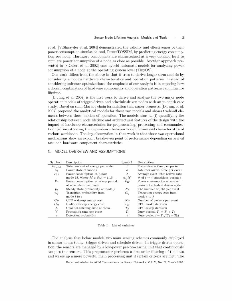
3. MODEL OVERVIEW AND ASSUMPTIONS

Symbol Description Symbol Description

ETotal Total amount of energy per node Z Transmission time per packetSi Power state of mode i σ Job inter arrival time per eventPM Power consumption at power λ Average event inter arrival rate

mode M , where M ∈ Si, i = 1...5 nij(t) # of i → j transitions during tPS Power consumption at asleep period PW Power consumption at awake

of schedule driven node period of schedule driven nodepj Steady state probability of mode j Nσ The number of jobs per eventpij Transition probability from Cij Transition energy cost from

mode i to j mode i to jCP CPU wake-up energy cost NP Number of packets per eventCR Radio wake-up energy cost TW CPU awake durationL Channel-listening time of radio TS CPU asleep durationY Processing time per event Tc Duty period, Tc = T1 + T2

u Detection probability d Duty cycle, d = T1/(T1 + T2)

Table I. List of variables

The analysis that below models two main sensing schemes commonly employedin sensor nodes today: trigger-driven and schedule-driven. In trigger-driven opera-tion, the sensors are managed by a low-power pre-processing unit that continuouslysamples the sensors. This preprocessor performs a first-order filtering of the dataand wakes up a more powerful main processing unit if certain criteria are met. The

Under submission to ACM Transactions on Sensor Networks, Vol. V, No. N, March 2007.


LEAP node [D.McIntire et al. 2005] and image sensors described in [T.Teixeiraet al. 2006] follow this model. In schedule-driven operation, the node’s sensors areconnected directly to the node’s main processor. To conserve energy, the processorfollows a schedule that alternates between a low-power mode (e.g sleep, deep-sleepor shutdown) and a short, full-power mode in which the processor (or its ADC)samples the sensors for interesting activity. If the desired event types are sensed, itproceeds to make the necessary computations and transmits the outcome with theradio if needed. The sentry nodes used in the Vigilnet project [T.He et al. 2006]follow this type of model. In this case the sentries are asleep most of the time, andperiodically wake up to sample for activity.

3.1 Assumptions

The models described in this paper make the following assumptions:

(1) The first-order statistical characteristic (mean value) of all random quantities(events, processing time, etc) is known by observation and experiment from theErgodic property.

(2) Event arrivals follow a Poisson distribution.(3) Processing and radio-transmission times are independent and identically dis-

tributed (i.i.d.) with arbitrary distribution.(4) When an event is detected, the node processes it and sends the information to

a base station (or another node) with probability α.(5) During the processing period, the CPU visits a limited number of low-power

states (e.g. idle state).(6) During the communication period, the radio visits a limited number of listen

(idle) states.(7) All power consumptions are constant during an operation and a fixed amount

of energy is required to turn on or off the CPU and radio.

The first three assumptions imply that the power state transitions may be mod-eled as a semi-Markov chain [S.M.Ross 1996] that can be used to compute a node’saverage power consumption and lifetime. While assumption 2 may not always holdtrue in all deployments a Poisson arrival rate is a representative model for manyapplications. For example, the number of people entering a building is a well knownexample of Poisson arrival [Ihler et al. 2006]. For the purposes of our analysis we ar-gue that the Poisson assumption is a reasonable choice because our main interest isto exercise the node hardware parameters that influence lifetime. Furthermore, byfixing the distribution of arrival events in our models we provide a common baselinefor the comparison of many platforms by exercising their features under the sameunderlying distribution. In order to include communication overhead in the lifetimeanalysis, the same communication paradigm is adopted for both the trigger-drivenand schedule-driven models as stated in assumption 4. The next two assumptions,5 and 6, related to the idle state of the CPU and listening state of the radio, arenecessary to more accurately describe the power consumption of those components.When an event is sensed by the node, the CPU will usually go to a full-power, ac-tive mode to perform some processing or additional sensing, but may alternate itwith a temporary lower-power state to conserve energy. This is accounted for inUnder submission to ACM Transactions on Sensor Networks, Vol. V, No. N, March 2007.


Trigger-Driven Node Schedule-Driven NodeMode Preprocessor Sensor CPU Radio Sensor CPU Radio

S0 – – – – Off Off OffS1 On Off Off Off – – –S2 On On On Off On On OffS3 On On On TX On On TXS4 On On Idle Off On Idle OffS5 On On On RX On On RX

Table II. Power state description

assumption 5. Meanwhile, it is common for MAC protocols to listen to the radiochannel before any transmission, to avoid packet collisions [B.Bougard et al. 2005].For this we have introduced assumption 6. We also emphasize that our modelsfocus on node-level behaviors by examining the parameters of the node hardwareunder different event arrival rates. Software and network level optimizations aretherefore not considered in this analysis.

3.2 Node Power Modes and Variables

Our analysis considers a simplified version of the power modes available on sen-sor nodes, eliminating some of the impractical modes. The modes considered aredescribed in Table II. To develop our models we also introduce a set of variables.These are described Table I. Our notation also uses a bar to denote expected value(i.e the expected value of the variable A is A).

4. LIFETIME MODELS

In this section, we will show that each sensor node can be modeled by an em-bedded semi-Markov Chain. Typically a sensor node performs a predefined set offunctions for each sensing an event: mainly sensing, computation, and communica-tion. Therefore, the instantaneous power consumption follows a certain pattern andusually the level is deterministic during the node lifetime unless an adaptive powercontrol mechanism is exploited. The amount of time spent at each power level isusually a random quantity that varies at each instance of the event and in manycases the mean and standard deviation are fixed. The distribution of the randomtime mainly depends on the event characteristic, i.e event arrival time and eventduration. In order to analyze the asymptotic pattern of energy dissipation at sensornode, we must consider both of power level and random time simultaneously. Wecan describe the pattern very accurately by a semi-Markov model assuming Poissonevent arrival. A semi-Markov process is one that changes states in accordance witha Markov chain but takes a random amount of time between changes.

Let X(t) denote the power state at time t. Then a change from state X(t), t ≥ 0does not solely depend on the present state, but also the length of time that hasbeen spent in that state. This characterizes a semi-Markov chain, as states changein accordance with a Markov chain but there is a random length of time betweenthe changes. Let Hi denote the distribution of time that the semi-Markov processspends in state i before making a transition, and let the mean be µi =

∫∞0

xdHi(x).With Xn denoting the nth state visit, Xn, n ≥ 0 becomes a Markov chain withtransition probabilities pij . It is also called the embedded Markov chain of the



Tx Time,ZProc. Time,Y

Inter-arrival Time,X

α1S

2S3S 1S 2S

3S

1

1

1 α−

α

Interrupt to CPU

Process Complete

Tx Radio OnRadio Off

(a) (b)

Fig. 1. (a) Power profile of simplified trigger-driven node model, (b) Semi-Markov chain of sim-plified trigger-driven node model.

semi-Markov process [S.M.Ross 1996]. Let Tii denote the time between successivetransitions into state i and let µii = E[Tii]. If the semi-Markov process is irreducibleand if Tii has nonlattice distribution with finite mean, then

pi ≡ limt→∞

P [X(t) = i|X(0) = j] = limt→∞

Tt

t, (1)

where Tt is the amount of time in i during [0, t], exists and is independent ofthe initial state, j. In other words, pi equals the long-run proportion of time instate i (the time spent in i over the combined time spent in all states). Supposefurther that the embedded-Markov chain Xn, n ≥ 0 is positive recurrent. Then astationary probability exists, which is the frequency of visiting each state for infinitetime duration . Let its stationary probability be πj , j ≥ 0. Then πj is the uniquesolution of

πj =∑

i

πipij ,∑

j

πj = 1 (2)

and πj can be interpreted as the proportion of transitions into state j (over thesum of all state transitions). Then the following theorem holds

pi =µi

µii=

πiµi∑j πjµj

(3)

Using equations (2) and (3), one can compute the long-run proportion of time instate i.

4.1 Trigger-Driven Lifetime Model

Figure 1a shows the simplest power model. In this model, the sensor node hasonly three states, which can be represented by the semi-Markov chain in Figure 1b.This model does not account for any Idle or Listening modes on the CPU or radio,respectively. However, in reality the CPU and radio often enter Idle mode duringthe processing and communication stages. For example, when an event is detected,the CPU has a choice of either processing the data, or deciding to drop it (or quicklystore it for later). In these situations, the CPU may go back into an idle state towait for the next job. Meanwhile, radios tend to spend considerable energy listeningUnder submission to ACM Transactions on Sensor Networks, Vol. V, No. N, March 2007.


2S 4S

Job enters

Job completed

3S 5S

Tx completed

Channel Idle

2S

σ

Nσ

4S

1λ−

L

PN5S 3S

Z

2S 4S

1S

Preprocessing Stage Processing Stage

Communication Stage

α

1 α−

1

1Triggered by Event

Job enters

Job completed

3S 5S

Tx completed

Channel Idle

Monitoring Event

(a) (b)

Fig. 2. (a) Power profile of complete trigger-driven node model, (b) Semi-Markov chain of completetrigger-triven node model.

to the channel before any actual transmission due to impositions of the underlyingMAC protocol. In IEEE 802.15.4, for instance, less than 50 percent of energyis spent for actual transmission, and listening activity accounts for more than 40percent of energy consumption [B.Bougard et al. 2005]. To take these factors intoaccount, Figure 2a deals with the addition of the idle and listening states of theCPU and radio. The updated semi-Markov chain in Figure 2b shows that eachprocessing and communication stage contains a two-state embedded chain.

For now, consider the simplest power model ( Figure 1(b) ). By applying (2) tothe semi-Markov chain, the following equations are obtained:

∑1≤j≤3

πj = 1, π

0 1 01− α 0 α

1 0 0

= π (4)

where π = [π1 π2 π3]. The solution of (4) gives π1 = π2 = 12+α and π3 = α

2+α .Therefore, the steady state probability of each state can be computed applying (3):

p1 =X

D(α), p2 =

Y

D(α), p3 =

αZ

D(α)(5)

where D(α) = X + Y + αZ.Given a long enough time period, T , the total time spent at state i can be

approximated as limT→∞ Ti = Tpi. Therefore, the total energy spent at state iis ESi = Tpi × PSi , for i ∈ {1, 2, 3}, and the transition energy cost from state ito j during T can be obtained as ESij = Cijnij(T ). However, only the CPU andradio wake-up costs (CP and CR, or, in ESij notation, ES12 and ES23) need tobe taken into consideration since the sleep cost is negligible in comparison. Theaverage number of transitions between 1 and 2, and 2 and 3 during period T canbe computed as n12 = π2T

D(α) , and n23 = π3TD(α) respectively.

Since the total amount of energy spent at each state, ESi , and the transitionenergy, ESij , cannot exceed the energy resource, Etotal, the following inequalityholds:



∑1≤k≤3

ESk+ ES12 + ES23 ≤ Etotal (6)

By solving inequality (6), the asymptotic node lifetime follows.

TL(λ) ≤ [1 + λ(Y + αZ)]ETotal

PS1 + λ(Y PS2 + αZPS3 + CD), CD =

CP + αCR

1 + α(7)

The updated semi-Markov chain in Figure 2 shows each processing and communi-cation stage contains a two-state embedded chain. The average power consumptionand sojourn time in these two-state chains can be computed as follows:

PProc =σPS4 + Y PS2

σ + Y, TProc = (σ + Y )Nσ (8)

PComm =LPS5 + ZPS3

L + Z, TComm = (L + Z)NP (9)

The final equation for average node lifetime can be computed by applying (8)and (9) to (7), resulting in:

TL(λ) ≤ 1 + λ[(σ + Y )Nσ + α(L + Z)NP ]ETotal

PS1 + λ[(σPS4 + Y PS2)Nσ + α(LPS5 + ZPS3)NP + CD](10)

(7) and (10) can be expressed more compact form as shown in

TL(λ) ≤ [1 + λKT ]ETotal

PS1 + λKE(11)

In (11), KT and KE represent the average time and energy spent for a sensedevent respectively. Typically, KE � PS1 and λ � 1sec−1. As shown in thedenominator of (11), the power component can be roughly broken down into twoparts: λKE , the average power spent for computation and communication persensed event; and PS1 , the power spent to monitor the events. It can be easilyfound that a sensor node spends more power monitoring an event than processingit at λ ≤ PS1

KE. The average steady-state power consumption of the trigger-driven

sensor node is simply given as:

PST,td(λ) =PS1 + λKE

[1 + λKT ](12)

For the simplest power model, Figure 1a, KT and KE are given as:

KT = Y + αZ, KE = Y PS2 + αZPS3 +CP + αCR

1 + α(13)



0S

Communication Stage

3S

4S5S

Processing Stage

2S

WT STCT

Missed Event

Detected Event1λ−

PCRC

Communication Stage

2S 4S4S

Idle Stage Processing Stage

α

1 α−

1

1Event

Detected

Job enters

Job completed

3S 5STx completed

Channel Idle

Monitoring Event

(a) (b)

Fig. 3. (a) Schedule-driven node power profile, (b) Power state transition during wake-period.

By taking into consideration the average power consumption and sojourn timein these two-state chains as shown Figure 2b, KT and KE are given as:

KT = (σ + Y )Nσ + α(L + Z)NP

KE = (σPS4 + Y PS2)Nσ + α(LPS5 + ZPS3)NP +CP + αCR

1 + α

(14)

4.2 Schedule-Driven Lifetime Model

Let k be the total number of duty cycles during the node’s entire lifetime, and eachεi the residual processing time after the ith awake state of the node. Additionally,let TW be the length of time when the node is awake. Then the average nodelifetime is obtained as following:

∑0≤i≤k

((TW + εi)PW,i + (TS − εi)PS,i + CP ) ≤ ETotal (15)

where PW,i and PS,i denote average power consumption of awake and asleepperiods during cycle i respectively. Note that each PW,i incorporates the powerexpenditure of four power states: S2, S3, S4 and S5. As for the power computation,the schedule-driven node performs the same function as the trigger-driven nodewhen an event occurs during the awake period (Figure 3). Therefore, given a longenough timespan, the average power consumption of the node during the activeperiod (PW,i) can be approximated by replacing in (12) the preprocessing powerwith idle power, and setting CP = 0. The result is shown below:

limi−→∞

PW,i = PW (λ) =PS2 + λK ′

E

1 + λK ′T

(16)

In (16), K ′T and K ′

E represent the average time and energy spent for a sensedevent respectively during awake period. Typically, K ′

E > PS2 and λ � 1sec−1. Asbefore, the nominator of (16) shows the power component during the awake periodcan be roughly broken down into two factors, namely λK ′

E , the average power spentfor computation and communication per sensed event, and PS2 , the static powerspent during the awake period. It can be easily found that a sensor node spends



0

PS

C

CPT

+

0( )W SSlope P Pλ= −

, ( )ST tdP λ

, ( )ST sbP u

0

0

, ( ) ( )

( )

DST td S

c

W S

CP PT

P P

λ

λ

− +

−

*u u

Average P

ower

Consum

ption

Average Detection

Probability

STP Trigger driven node

Schedule driven node

Fig. 4. Tradeoff Diagram: Power versus Average Detection Probability

more power for the idle state than processing events at λ ≤ PS2K′

E.

For the awake period of the schedule-driven power model, (Figure 1b) K ′T and

K ′E are given as using (14):

K ′E = (σPS4 + Y PS2)Nσ + α(LPS5 + ZPS3)NP +

αCR

1 + α

K ′T = (σ + Y )Nσ + α(L + Z)NP

(17)

Using the fact that PS,i(t) is constant (PS,i ≡ PS0), the average node lifetimecan be obtained by applying (16) to equation (15):

TL ≈ (TW + TS)k ≤ ETotal(TW + TS)[TW PW (λ) + TSPS0 + (PW (λ)− PS0)ε + CP ]

(18)

Since it is typically the case that TW � ε, the term (PW (λ)−PS0)ε can often beignored as TW PW (λ) � εPW (λ) ≥ ε(PW (λ)− PS0).

4.3 Trigger-Driven and Schedule-Driven Comparison

To meaningfully compare the two models, the event detection probability also needsto be considered. For the trigger-driven case, the sensor and preprocessor arealways on, so we can assume that event detection happens with probability one.This comes at a price, of course, of added power cost for the preprocessor. Theschedule-driven scheme, however, takes no such toll on power, but does so at theexpense of event detection probability. In most of cases, detection probability,u, is a monotonically increasing function of duty cycle, d, i.e u = f(d) wheref(u1) ≤ f(u2) iff u1 ≤ u2. For example, [T.He et al. 2006] and [Q.Cao et al. 2005]show that detection probability in the target tracking application is a non-linearincreasing function of sentry node duty cycle. For analytical simplicity, we assumethat all events that do not coincide with the node’s duty-cycle remain undetected.To compare, let us define two random variables U and V to describe the number ofUnder submission to ACM Transactions on Sensor Networks, Vol. V, No. N, March 2007.


Poisson sensor events during TW and Tc respectively. Then the average detectionprobability, E

[UV

], can be computed as:

E

[U

V

]=

∑0≤v≤∞

E

[U

v

∣∣∣∣ V = v

]PV (v) =

∑0≤v≤∞

1v

[vTW

Tc

]PV (v) =

TW

Tc= d (19)

The second equality of Equation (19) comes from the fact that P (U = u|V = v)has a binomial distribution, B(v, d), where d = TW

Tc. As shown in Equation (19),

the detection probability is simply the duty cycle of the schedule-driven node.Therefore, we can express the trade-off diagram between the trigger-driven andschedule-driven schemes as a function of the detection probability u (shown inFigure 4), where the node lifetime of the schedule-driven node follows the equation:

TL(u) ≤ ETotal

(PW (λ)− PS0)u + (PS0 + CP

Tc)

(20)

From (20), the average steady-state power consumption of the schedule-drivennode can be found:

PST,sb(u) = (PW (λ)− PS0)u +(

PS0 +CP

Tc

)(21)

By superimposing the two average power consumption formulas (Equations (21)and (12)), we can obtain a trade-off diagram as Figure 4. The thick line denotesthe lowest-power choice for a given detection probability. The two curves meet

at u∗ =PST,td(λ)−(PS0+

CPTc

)

PW (λ)−PS0. The figure shows that for an application that allows

the use of sensors with detection probability smaller than u∗, the schedule-drivenscheme is a sound choice. For events with larger arrival rates, u∗ gets shiftedto the right, further favoring the schedule-driven scheme for frequent, non-criticaldetections. Otherwise, if the application demands high-accuracy, the trigger-drivenscheme is a better alternative. Of course, multiple nodes with complementaryschedules may reduce the number of events that are globally missed, but such anetwork-wide power analysis is out of the scope of this paper.

5. VALIDATION

The numerical correctness of our models was validated through simulation. Usingthe empirical iMote2 measurements (will be shown in section 6), the two sensingschemes (scheduled and trigger-driven) were simulated in MATLAB. Basically, oursimulator tracks energy dissipation of a node over large time window at 1 secondtimesteps by subtracting the accumulated power consumption from a given energyresource. The simulator consists of an Event Generator (EG), a Processing Element(PE), and a communication unit (CU). According to our assumption 2 (section 3),the EG triggers the PE after elapsing exponential random time from a previousevent. The PE alternates a busy state (actively processing information) and an



idle state. The CU also alternates a transmission state and a listening (idle) state.The workload simulated on the PE and CU is not taken from a real application,but modeled by a parameterized workload with properties represented by inputparameters: processing time, idle time, number of jobs for the PE and transmissiontime, listening time, number of packet for the CU. A workload taken from realapplication would result in more accurate simulation. However, the result wouldnot be representative for the broad spectrum of application in wireless sensor net-works. For example, the workload for surveillance application [T.He et al. 2006]shows different characteristics from the one for environmental data collection ap-plication[Mainwaring et al. 2002]. Thus workload measured from our applicationcannot not be generalized to other applications. The parameterized workload canbe easily manipulated to simulate different workload characteristics from variousapplications . We believe that parameterized workloads can be used to determinethe initial values of architectural parameters. A real workload can then be usedto tune these parameters. All timing (e.g processing or transmission time) andcounting numbers (e.g the number of jobs or packets) can be specified as constantsor random variables. The simulator supports three distributions: exponential, uni-form, and normal.

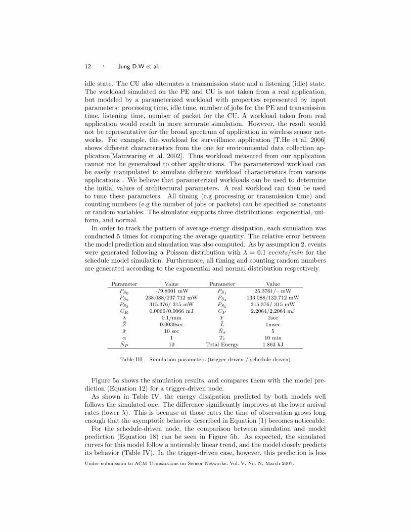
In order to track the pattern of average energy dissipation, each simulation wasconducted 5 times for computing the average quantity. The relative error betweenthe model prediction and simulation was also computed. As by assumption 2, eventswere generated following a Poisson distribution with λ = 0.1 events/min for theschedule model simulation. Furthermore, all timing and counting random numbersare generated according to the exponential and normal distribution respectively.

Parameter Value Parameter Value

PS0 –/9.8001 mW PS1 25.3761/– mWPS2 238.088/237.712 mW PS4 133.088/132.712 mWPS3 315.376/ 315 mW PS5 315.376/ 315 mWCR 0.0066/0.0066 mJ CP 2.2064/2.2064 mJλ 0.1/min Y 2secZ 0.0039sec L 1msecσ 10 sec Nσ 5α 1 Tc 10 min

NP 10 Total Energy 1.863 kJ

Table III. Simulation parameters (trigger-driven / schedule-driven)

Figure 5a shows the simulation results, and compares them with the model pre-diction (Equation 12) for a trigger-driven node.

As shown in Table IV, the energy dissipation predicted by both models wellfollows the simulated one. The difference significantly improves at the lower arrivalrates (lower λ). This is because at those rates the time of observation grows longenough that the asymptotic behavior described in Equation (1) becomes noticeable.

For the schedule-driven node, the comparison between simulation and modelprediction (Equation 18) can be seen in Figure 5b. As expected, the simulatedcurves for this model follow a noticeably linear trend, and the model closely predictsits behavior (Table IV). In the trigger-driven case, however, this prediction is lessUnder submission to ACM Transactions on Sensor Networks, Vol. V, No. N, March 2007.


(a) (b)

Fig. 5. (a) Energy dissipation of trigger-driven model, (b) Energy dissipation of schedule-drivenmodel.

Trigger-Driven Node

λ(ev./min) model (sec) simulation (sec) relative error

0.1 1.7650e+004 1.9723e+004 11.74%0.01 4.5509e+004 4.6706e+004 2.62%0.001 6.8761e+004 6.9121e+004 0.5233%

Schedule-Driven Node

u model (sec) simulation (sec) relative error

0.1 8.3302e+004 8.0747e+004 3.0673 %0.5 2.5659e+004 2.5749e+004 0.3505%0.9 1.5165e+004 1.5607e+004 2.9152%

Table IV. Relative error of lifetime between model prediction and simulation

Processing and Communication UnitImote2

Preprocessor

PIR Motion Detector

PIC microcontroller

OV7649Camera

PXA 27x

DMACC2420 Radios

Image Data

MotionData

Wake-Up Signal

EventSensing Motion

Sensing Image

CentroidData

To BaseStation

Turn On

(a) (b)

Fig. 6. (a) iMote2 node with a COTS camera board, (b) Trigger-driven sensor node with iMote2fitted with a PIC microcontroller and PIR motion sensor

accurate for largest (0.9) and lowest (0.1) duty cycles compared to the median dutycycle (0.5). This is because the residual processing time ε becomes significant forthe awake period (ε/T1) at lower duty cycle while the residual processing time εbecomes significant for asleep period (ε/T2) at higher duty cycle.



6. CASE STUDY: USING THE MODELS TO CHARACTERIZE AND MAKE DECI-SIONS ABOUT A CAMERA SENSOR NODE

To demonstrate the usefulness of the models derived in the previous sections, we nowdemonstrate their application in the decision-making process deriving the designof an experimental camera sensor node designed for the BehaviorScope project atYale. Our goal is to decide whether it makes sense to develop an improved versionof the camera node shown in Figure 6a. This camera node is an Intel iMote2[L.Nachman 2005] coupled with a custom camera board we have designed with acommercial, off-the-shelf (COTS) image sensor, Omnivision’s OV7649. The nodeis powered by three AAA batteries (1150mAh capacity). The alternative designwe are considering is a new camera board that supports a wakeup preprocessormechanism comprised of a passive infrared (PIR) sensor for detecting motion and asmall 8-bit PIC 10F200 microcontroller to act as a preprocessor. This configuration(described in Figure 6b) would allow the node to follow a trigger-driven mode ofoperation. Instead of periodically sampling the camera to detect activity, with thisimprovement the PXA 271 processor onboard the iMote2 will wait in a low-powerstate until triggered by the PIC-based preprocessor that is always kept on for asmall energy overhead (Mode S1 in Table VII). In this state, the preprocessor willapply a thresholding algorithm to the samples it collects from the PIR sensor. Ifthe observed motion exceeds a predefined value, the preprocessor will power upthe iMote2 and camera board to acquire and process the images. If the imageprocessing reveals something of interest, the node then transmits the informationto a basestation. These transmissions take place with probability α.

0 5 10 15 20 25 300

50

100

150

200

250

300

350

400

Time(sec)

Pow

er(m

W)

0 1 2 3 4 5 6 7 8 9 10 11 12 13 14 15 16 17 18 19 20 21 22 23 24 25 26 27 28 29 30

0

100

200

300

400

500

600

700

Ene

rgy(

mJ)

TransmittingCentroids

Processing Cetorids

Preparing Sleep Mode:Disable 13M oscillator

iMote2 in Deep Sleep

Waking upiMote2

27 27.05 27.1 27.15 27.2 27.25 27.3 27.35

280

290

300

310

320

330

340

350

Time(sec)

Pow

er(m

W)

Radio Wakeup

ChannelListening

PacketTransmission

2.6 2.62 2.64 2.66 2.68 2.7 2.72 2.74 2.76 2.78 2.8

264

266

268

270

272

274

276

278

Time(sec)

Pow

er(m

W)

CapturingImage

TransferringImage

ExtractingCentorid

Fig. 7. Power profile of trigger driven iMote2



Parameter Value Parameter Value

λ 0.1/min Y 2sec∗

Z 3.8msec L 0 msecσ 0 min Nσ 1α 1 Tc 10 min

NP 1 Total Energy 18.63 kJ

Table V. Reference scenario, measured (∗)

To provide more concrete numbers in our case study, we set up the camera nodeto act as a simple single target localization device. An event is defined as thecomplete trajectory of human centroid within view of the camera on our sensornode. In this setting, the camera sensor node performs the following functions inorder.

(1) When a person enters the camera’s field-of-view, the preprocessor wakes up theiMote2 and camera (only for the trigger-driven node).

(2) When awake, the iMote2 continually computes the location of the person at afrequency of 8Hz (8fps) until the person exits the coverage area of the camera.

(3) Once the person is out of the sensing range, the node transitions back into thelow power mode after sending a stream of locations to the base station.

Figure 7 shows the measured power profile pattern for each imote2 accordingto our functional description. In this task, the PXA processor performs motiondifferencing between consecutive frames captured by the camera. The location ofthe target is the centroid of the pixels that moved between two consecutive frames.Each centroid computed is stored in the memory and the node transmits the storedcentroid information to the base station with probability 1 (i.e α = 1). 1. Eachcentroid information consists of 2 bytes of location information, (X,Y) grid and 4bytes of time information, real time clock. Here we defined the event as follows.

— The event is defined as the complete trajectory of human centroid in the rangeof camera sensor.

— The event arrival rate is defined as the frequency a person enters the camerafield of view. Therefore, it is roughly computed as the number of people observedby camera sensor divided by total observation time.

— The event duration is defined as the time interval a person spends in the camera’sfield of view.

— The event is said detected if and only if there is no missed centroid during theevent duration. Otherwise, it is said missed.

In our experiments, typically event duration is roughly 2 seconds. From ourevent definition, processing time is actually the same as event duration, and anyincomplete trajectory (set of centroids) of a person is considered a missed event(hard-decision). For example, if a person enters the camera view, and 1 sec later anode wakes up and observes only half of the trajectory, then the event is considered

1This role is simplified and used for illustrative purposes only. More complex roles can be describedusing our tool presented in section 7



missed. For real-time computation, the node may transmit the centroids as soonas they are acquired. We do however note that whether the centroids are sentimmediately or left for transmitting later is not of relevance to our models, as long asthe energy consumption of both cases is still the same. From a lifetime perspective,the summation of the energy spent at each stage will be same regardless of theprocessing order. The time between capturing a frame and extracting a centroid is123msec/centroid. Therefore, a node generates a total of roughly 16 centroids perevent and the total amount of information per event is 96 bytes. With a packetsize of 119 bytes (including a 23 byte packet header) transmitted at the rate of 250kbps, the packet transmission takes 3.8msec. As a reference scenario, we set thesystem parameter values as specified in Table V.

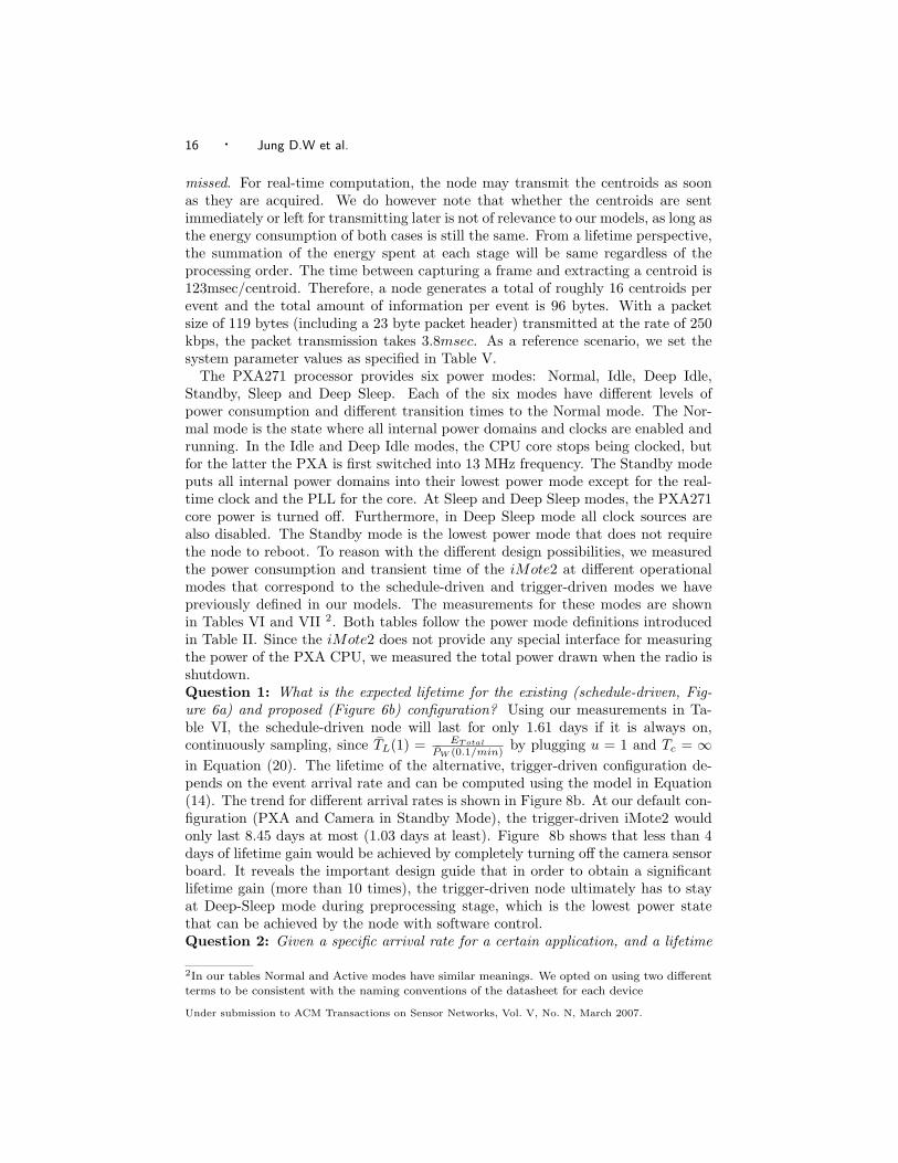
The PXA271 processor provides six power modes: Normal, Idle, Deep Idle,Standby, Sleep and Deep Sleep. Each of the six modes have different levels ofpower consumption and different transition times to the Normal mode. The Nor-mal mode is the state where all internal power domains and clocks are enabled andrunning. In the Idle and Deep Idle modes, the CPU core stops being clocked, butfor the latter the PXA is first switched into 13 MHz frequency. The Standby modeputs all internal power domains into their lowest power mode except for the real-time clock and the PLL for the core. At Sleep and Deep Sleep modes, the PXA271core power is turned off. Furthermore, in Deep Sleep mode all clock sources arealso disabled. The Standby mode is the lowest power mode that does not requirethe node to reboot. To reason with the different design possibilities, we measuredthe power consumption and transient time of the iMote2 at different operationalmodes that correspond to the schedule-driven and trigger-driven modes we havepreviously defined in our models. The measurements for these modes are shownin Tables VI and VII 2. Both tables follow the power mode definitions introducedin Table II. Since the iMote2 does not provide any special interface for measuringthe power of the PXA CPU, we measured the total power drawn when the radio isshutdown.Question 1: What is the expected lifetime for the existing (schedule-driven, Fig-ure 6a) and proposed (Figure 6b) configuration? Using our measurements in Ta-ble VI, the schedule-driven node will last for only 1.61 days if it is always on,continuously sampling, since TL(1) = ET otal

PW (0.1/min)by plugging u = 1 and Tc = ∞

in Equation (20). The lifetime of the alternative, trigger-driven configuration de-pends on the event arrival rate and can be computed using the model in Equation(14). The trend for different arrival rates is shown in Figure 8b. At our default con-figuration (PXA and Camera in Standby Mode), the trigger-driven iMote2 wouldonly last 8.45 days at most (1.03 days at least). Figure 8b shows that less than 4days of lifetime gain would be achieved by completely turning off the camera sensorboard. It reveals the important design guide that in order to obtain a significantlifetime gain (more than 10 times), the trigger-driven node ultimately has to stayat Deep-Sleep mode during preprocessing stage, which is the lowest power statethat can be achieved by the node with software control.Question 2: Given a specific arrival rate for a certain application, and a lifetime

2In our tables Normal and Active modes have similar meanings. We opted on using two differentterms to be consistent with the naming conventions of the datasheet for each device



CPU Camera RadioMode PXA271 OV7649 CC2420 Total

S0 Deep Sleep Standby Shutdown

1.8mW 8mW 144nW 9.8mW

CP 48.63mJ - 691pJ 48.63 mJ

252msec - 970µsec 253msec

S2 Normal Active Idle

193mW 44mW 712µW 237.7mW

S4 Deep Idle Active Idle

88mW 44mW 712µW 132.7mW

CR - - 6.63µJ 6.63µJ

- - 194µsec 194µsec

S3 Normal Active TX

193mW 44mW 78mW 315mW

S5 Normal Active RX

193mW 44mW 78mW 315mW

Table VI. Typical power-consumption specifications of schedule-driven camera sensor node(iMote2) at 104 MHz CPU Core frequency, 4MHz PIC and 0dBm TX Power

Preprocessor CPU Camera RadioMode Motion Sensor PIC10F200 PXA271 OV7649 CC2420 Total

S1 On On Standby Standby Shutdown

3.6µW 340µW 17mW 8mW 144nW 25.34mW

CP - - 2.2mJ - 114nJ 2.2mJ

- - 11.432msec - 970µsec 12.4msec

S2 On On Normal Active Idle

3.6µW 340µW 193mW 44mW 712µW 238.05mW

S4 On On Deep Idle Active Idle

3.6µW 340µW 88mW 44mW 712µW 133.05mW

CR - - - - 6.63µJ 6.63µJ

- - - - 194µsec 194µsec

S3 On On Normal Active TX

3.6µW 340µW 193mW 44mW 78mW 315.34mW

S5 On On Normal Active RX

3.6µW 340µW 193mW 44mW 78mW 315.34mW

Table VII. Typical power-consumption specifications of trigger-driven camera sensor node(iMote2)at 104 MHz CPU Core frequency, 4MHz PIC and 0dBm Tx Power on a CC2420 radiorequirement, what is the maximum power a pre-processor(and sensor) can consume?To obtain the power budget for the pre-processor we need to solve for PS1 of thetrigger-driven model in (11). The lifetime trend at different event arrival times asa function of preprocessor power is shown in Figure 8c.Question 3: If we don’t build the proposed board and use a duty-cycle instead,what is the expected lifetime for a certain detection probability? We can answerthis question by plugging in the detection probability u in the lifetime model forthe schedule-driven node described by Equation (20). The expected lifetimes fordifferent detection probabilities are shown in Figure 8a.Question 4: Suppose we had an ideal sensor preprocessor (power cost=0) whatwould be the lifetime of the node at a certain arrival rate? This trend is shown



0 0.1 0.2 0.3 0.4 0.5 0.6 0.7 0.8 0.9 10

5

10

15

20

25

Detection Probabilty

Life

time

(day

s)

10-3 10-2 10-1 100 101 102100

101

102

Life

time

(day

s)

Event Inter-Arrival Rate (1/min)

iMote2 Deep SleepCamera board Off

PXA Standby ModeCamera board Off

PXA Standby ModeCamera Standby

94.15

12.338.45

(a) (b)

0 10 20 30 40 50 60 70 80 90 1000

5

10

15

20

25

Preprocessor (mW)

Life

time

(day

s)

λ=1/10minPXA in Standby Mode

λ=0PXA in Standby Mode

λ=∞PXA in Standby Mode

λ=0iMote2 in Deep-Sleep Mode

10-3 10-2 10-1 100 1010

5

10

15

20

25

Event Inter-Arrival Rate (1/min)

Life

time

(day

s)

Schedule-Driven iMote2Trigger-Driven iMote2

Preprocessor=0 mWPXA in Standby Mode

Preprocessor=0 mWiMote2 in Deep Sleep Mode

Duty Cycle=0iMote2 in Deep Sleep Mode

Duty Cycle=0PXA in Standby Mode

(c) (d)

0 0.1 0.2 0.3 0.4 0.5 0.6 0.7 0.8 0.9 10

20

40

60

80

100

120

140

160

180

200


Life

time

(day

s)

10-3 10-2 10-1 100 101 1020

100

200

300

400

500

600

700

Event Inter-Arrival Rate (min-1)

Life

time

(day

s)

(e) (f)

Fig. 8. a) Lifetime trend versus detection probability for question 1, b) Lifetime trend versusarrival rate for question 1, c) Lifetime trend for question 2, d) Lifetime trend for question 3, e)Lifetime trend versus detection probability for the sentry node described in VigilNet, f) Predictedhypothetical lifetime trend versus arrival rate for the sentry node described in VigilNet

in Figure 8d. If we use Standby mode as the lowest power mode, in a trigger-driven configuration, the node will last for only 8.62 days! Also, if we entirelydisable the preprocessor, the node will operate as in the schedule-driven modelwith duty-cyle=0, missing all events. Even so, the node lifetime is only 8.62 days,indicating that we should try to operate at power levels lower than the Standbymode. Comparing Figure 8c and Figure 8d, we notice that just lowering the powerconsumption of the preprocessor does not impact the lifetime trend of the trigger-Under submission to ACM Transactions on Sensor Networks, Vol. V, No. N, March 2007.


driven node since PS1 is heavily dominated by the power consumption of the cameraboard and PXA at Standby mode. Indeed, our computation shows that for rareevents the lifetime increases to 94 days, with the camera board off and the iMote2in Deep Sleep mode (Figure 8b). Much to our surprise, our models have shownthat the addition of a preprocessor and trigger-driven operation will not providesubstantial lifetime gains. This is mainly due to the high power consumption in theStandby mode of the PXA and camera. The trends also indicate that it is unlikelyto significantly improve lifetime by manipulating the processor power modes alone.A better strategy would be to consider mechanisms that disconnect the entire nodefrom the power supply as suggested in [D.Lymberopoulos and A.Savvides 2005].According to our models, the use of such a mechanism would increase the lifetimeof the schedule-driven node to 552 days ( since TL(1) = ET otal

PS0by plugging u = 0

and Tc = ∞ in Equation (20) ), a large improvement over the currently predicted8.45 days for a non-ideal preprocessor (see Figure 8d).

As a sanity check, we also used our model to predict the lifetime of the Micaznodes used in the Vigilnet project [T.He et al. 2006]. Using our model, we computedthe expected lifetime of a sentry node to be about 442 hours (18.5 days) as shownin Figure 8e. According to [T.He et al. 2006], a sentry node will last 90 days with arole rotation of 4-5 nodes and 25% of sentry duty cycle. Multiplying our predictionby 5 to account for role rotation, our model will anticipate a lifetime of 92.5 days,an estimate that is very close to the lifetime of the real deployment reported bythe authors of [T.He et al. 2006]. Furthermore, Figure 8f shows that the lifetimeof the sentry node will significantly increase if we convert it into a trigger-drivennode using the same preprocessor as before.3 Such a high lifetime gain comes fromthe fact that the power consumption of the sentry node at Sleep state is extremelylow (42 µW).

7. CAPTURING THE MODELS INTO A TOOL

To allow sensor node users and designers to use our models to drive design anddevelopment, we have developed a MATLAB toolkit, MATSNL. This tool imple-ments the trigger-driven and schedule driven models as well as the discrete-eventsimulation used to validate them (used for simulation in section 5). Users can en-ter new specifications for node architectures and application profiles. MATSNLprovides a set of commands for analyzing node lifetimes, compare platform perfor-mance for different application profiles and compute power budgets for new sensorpre-processors, radios and processors. This section provides a brief demonstrationof the tool using four popular sensor nodes, Intel’s iMote2, Yale’s XYZ, Crossbow’sMicaz and Moteiv’s Telos. The MATLAB code for the tool is publicly availableand can be found at: http://www.eng.yale.edu/enalab/aspire.htm.

7.1 Tool Organization

MATSNL is organized into three main components: configuration, analysis andsimulation. Configuration specifies the properties of each platform as previously

3This is a hypothetical lifetime since [T.He et al. 2006] does not consider a trigger-driven sentrynode



described in Table I. Application profiles are defined by the event arrival rate,duty-cycle and sometimes detection probability. The analysis part of the tool im-plements the models described in the sections 4.1 and 4.2. As we will describe lateron, the analysis and comparison results are obtained by applying a given config-uration to the models. The simulation component is independent of the analysiscomponent and runs a discrete event simulation on the parameters provided by theconfiguration component. The simulation first generates an event trace and thenexercises the different power modes of the platform according to the trace. Energyconsumption is computed by summing up the power consumed at each power modevisited and the corresponding transition overhead for each mode.

In its current form, MATSNL can perform four main functions:

(1) Analyse lifetime of trigger-driven and schedule-driven nodes (complf command).(2) Analyze power breakdown per mode (comppwr command)(3) Analyze preprocessor power (compprep command)(4) Execute a discrete event simulation for a given configuration (comp sim com-

mand).

The usage of the tool and the outcomes for each command are demonstratedwith illustrative examples in the next section.

7.2 MATSNL Usage

We now demonstrate the main features of MATSNL with example comparisons be-tween alternative sensor node designs. These examples are meant to be illustrativerather than exhaustive. The reader can study them in depth by changing differentparameters inside the tool. The first example examines the choice of processor fora wireless camera sensor node using numbers from the literature for the Micaz andXYZ nodes, and the iMote2 measurements we have taken during this work. Theapplication parameters and camera sensor board configuration used here are thesame as the ones we have described in our case study in section 6. The three nodes,iMote2, XYZ and Micaz have the same radio. We also assume that they have thesame sensor, and use their corresponding processor power consumptions and pro-cessing times to show how MATSNL could be used to study the effect of differentprocessors. The iMote2 has a PXA 271 processor, which we run at 104MHz andXYZ has an OKI ARM processor running at 58MHz and Micaz has an 8-bit AVRprocessor. To emphasize the processor effectiveness, we assume that for the sameimage processing and decision task the iMote2 processor takes 2 seconds, the XYZprocessor takes 4 seconds and the Micaz processor takes 48 seconds.

7.2.1 Lifetime comparison among platforms.A lifetime comparison between the three different configurations can be performed

by running a single MATSNL command, complf .

complf({′xyz′,′ imote2′,′micaz′}, [0.1 1], [5], 1, 30)

complf({′xyz′,′ imote2′,′micaz′}, [0.5], [1 1 ∗ 60 ∗ 24], 1, 30)

The first command above uses a duty cycle between 0.1 and 1 (for the schedule-driven node) an event interarrival time of 5 minutes, a communication probabilityUnder submission to ACM Transactions on Sensor Networks, Vol. V, No. N, March 2007.


0.2 0.4 0.6 0.8 1

10

20

30

40

50

60

70Li

fetim

e (d

ays)


Schedule driven XYZTrigger driven XYZSchedule driven iMote2Trigger driven iMote2Schedule driven MicazTrigger driven Micaz

10-1 100 101

50

100

150

200

Life

time

(day

s)

Event Arrival Rate (1/hour)

Schedule driven XYZTrigger driven XYZSchedule driven iMote2Trigger driven iMote2Schedule driven MicazTrigger driven Micaz

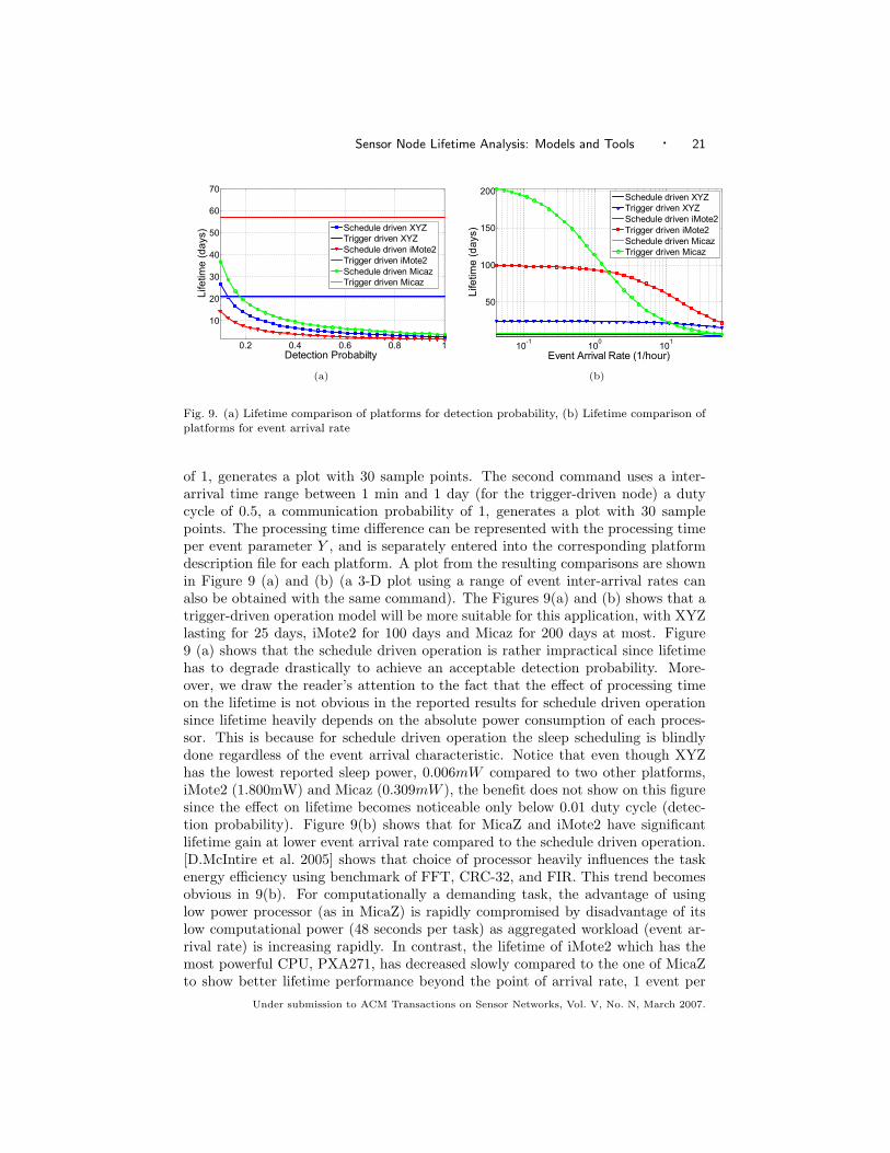
(a) (b)

Fig. 9. (a) Lifetime comparison of platforms for detection probability, (b) Lifetime comparison ofplatforms for event arrival rate

of 1, generates a plot with 30 sample points. The second command uses a inter-arrival time range between 1 min and 1 day (for the trigger-driven node) a dutycycle of 0.5, a communication probability of 1, generates a plot with 30 samplepoints. The processing time difference can be represented with the processing timeper event parameter Y , and is separately entered into the corresponding platformdescription file for each platform. A plot from the resulting comparisons are shownin Figure 9 (a) and (b) (a 3-D plot using a range of event inter-arrival rates canalso be obtained with the same command). The Figures 9(a) and (b) shows that atrigger-driven operation model will be more suitable for this application, with XYZlasting for 25 days, iMote2 for 100 days and Micaz for 200 days at most. Figure9 (a) shows that the schedule driven operation is rather impractical since lifetimehas to degrade drastically to achieve an acceptable detection probability. More-over, we draw the reader’s attention to the fact that the effect of processing timeon the lifetime is not obvious in the reported results for schedule driven operationsince lifetime heavily depends on the absolute power consumption of each proces-sor. This is because for schedule driven operation the sleep scheduling is blindlydone regardless of the event arrival characteristic. Notice that even though XYZhas the lowest reported sleep power, 0.006mW compared to two other platforms,iMote2 (1.800mW) and Micaz (0.309mW ), the benefit does not show on this figuresince the effect on lifetime becomes noticeable only below 0.01 duty cycle (detec-tion probability). Figure 9(b) shows that for MicaZ and iMote2 have significantlifetime gain at lower event arrival rate compared to the schedule driven operation.[D.McIntire et al. 2005] shows that choice of processor heavily influences the taskenergy efficiency using benchmark of FFT, CRC-32, and FIR. This trend becomesobvious in 9(b). For computationally a demanding task, the advantage of usinglow power processor (as in MicaZ) is rapidly compromised by disadvantage of itslow computational power (48 seconds per task) as aggregated workload (event ar-rival rate) is increasing rapidly. In contrast, the lifetime of iMote2 which has themost powerful CPU, PXA271, has decreased slowly compared to the one of MicaZto show better lifetime performance beyond the point of arrival rate, 1 event per



Event Inter-Arrival Rate (hour-1)

Pow

er b

reak

dow

n(m

W)

Trigger driven iMote2

0

2

4

6

8

Preprocessing

ProcessingIdle

TXRX

Trans.

10-2 100 102

Trigger driven XYZ

0

5

10

10-2 100 102

Trigger driven MicaZ

0

10

20

30

10-2 100 102

Fig. 10. Power breakdown comparison of multiple trigger driven platforms

hour. This trade-off point between two platforms with high-end processor and low-end processor implies the potential advantage of using multi processor core nodearchitectures (with high-end and low-end processor) so that platform exploits theprocessing power according to the computation efficiency. [D.McIntire et al. 2005]proposed LEAP platform adopting the architectures. Notice that the XYZ plat-form shows the lowest lifetime performance due to the highest preprocessing power,9.126mW compared to two platforms, MicaZ (1.024mW ) and iMote2 (2.176mW ).Although the smallest power mode of XYZ is deep sleep (0.006mW ), it cannot beused for the preprocessing stage since the RTC is the only interrupt source ableto wake up the processor unit. Therefore the lifetime bottleneck comes from thesecond lowest power mode, the standby mode where XYZ draws relatively largepower but is capable to wake up processor unit given the advent of event.

7.2.2 Power budget comparison among platforms.

A power budget/breakdown comparison between the three different configura-tions can be performed by running a single MATSNL command, comppwr.

comppwr({′imote2′,′ xyz′,′micaz′}, [−1], [1 1 ∗ 60 ∗ 24], 1, 30)

comppwr({′imote2′,′ xyz′,′micaz′}, [0.1 1], [1 ∗ 60], 1, 30)

The first command uses an inter-arrival time range between 1 min and 1 day (forthe trigger-driven node), a communication probability of 1 to generate a plot with30 sample points. The −1 stands for ’duty cycle is not defined’ by which it analyzespower budget only for trigger-driven case. The second command uses a duty cycleUnder submission to ACM Transactions on Sensor Networks, Vol. V, No. N, March 2007.


0.2 0.4 0.6 0.8 10

50

100

Duty Cycle

Pow

er b

reak

dow

n(m

W)

Schedule driven iMote2

Sleep

Idle

Processing

Tx

Rx

Trans.

0.2 0.4 0.6 0.8 10

20

40

60

Schedule driven XYZ

0.2 0.4 0.6 0.8 10

20

40

60Schedule driven MicaZ

Fig. 11. Power breakdown comparison of multiple schedule driven platforms

between 0.1 and 1, an inter-arrival time of 1 hour, a communication probability of1 to generate a plot with 30 sample points.

Figures 10 and 11 show the energy breakdown for the two models for the firstand second comppwr commands respectively. Figure 10 explains why the MicaZis not practical compared to the iMote2 at large workload (high arrival rate). Asshown in the Figure, the processing power per event in MicaZ rapidly outpaces theone in iMote2 so that the total average power consumption of MicaZ exceeds thatof iMote2 at points beyond the inter-arrival rate of 1 event per hour. Meanwhile forXYZ the preprocessing power takes most of portion of average power consumptionto degrade lifetime performance as shown Figure 9(b). Such a high preprocessingpower comes from large leakage current (3.5mA) of the CPU (Peripherals 1.69mA)and board (Radio board:0.883mA, Rest of the board: 0.927 mA)[D.Lymberopoulosand A.Savvides 2005]. Figure 11 shows that idle power dominates the power budget.In contrast, the other power budgets (such as sleeping and processing power) havenegligible effects on the lifetime. The Figure implies an important rule of thumb inthe energy conservation strategy of a schedule driven node for those platforms atmoderate event arrival rate: to minimize the idle power as much as possible.

7.2.3 Preprocessor Power analysis.

The lifetime and trade-off trend for different preprocessor power costs can becomputed by running a single MATSNL command, compprep.

compprep({′imote2′}, [0 50], [1 1 ∗ 60 ∗ 24], 0.6, 30)Under submission to ACM Transactions on Sensor Networks, Vol. V, No. N, March 2007.


0 10 20 30 40 500

20

40

60

80

100

120

Preprocessor (mW)

Life

time

(day

s)

Trigger driven iMote2

λ=60.00/hrλ=28.99/hrλ=14.01/hrλ=6.77/hrλ=3.27/hrλ=0.09/hr

14.17

14.17

106.33

106.33

14.17

14.17

14.17

14.17

14.17

14.17

14.17

14.17

14.17

14.17

14.17

7.64

7.64

7.64

7.64

7.64

7.64

7.64

7.64

5.23

7.64

7.64

5.23

5.23

5.23

5.23

5.23

5.23

5.23

5.23

5.23

3.98

5.23

3.98

3.98

3.98

3.98

3.98

3.98

3.98Schedule−Driven Favored

Trigger−Driven Favored


Eve

nt A

rriv

al R

ate

(1/h

our)

0.1 0.2 0.3 0.4 0.5 0.6 0.7 0.8 0.9 1

10−1

100

101

0 mW 5 mW10 mW

15 mW20 mW

25 mW 30 mW

35 mW40 mW

45 mW50 mW

(a) (b)

Fig. 12. (a) Lifetime trend of trigger driven iMote2 over preprocessor power budget, (b) Trade-offplot of trigger driven iMote2 over preprocessor power budget

0 5 10 15 20 25 30 35 40 45 500

50

Preprocessor (mW)Pow

er B

reak

dow

n(m

W)

λ=60.00/hr

PreprocessingNon-Preprocessing

0 5 10 15 20 25 30 35 40 45 500

50λ=28.99/hr

0 5 10 15 20 25 30 35 40 45 500

50λ=14.01/hr

0 5 10 15 20 25 30 35 40 45 500

50λ=6.77/hr

0 5 10 15 20 25 30 35 40 45 500

50λ=3.27/hr

0 5 10 15 20 25 30 35 40 45 500

50λ=0.09/hr

Fig. 13. Trade-off plot of trigger driven iMote2 over preprocessor power budget

The above command considers a preprocessor power range between 0mW and50mW ,a inter-arrival time range between 1 min and 1 day (for the trigger-drivennode), a communication probability of 0.6 to generate a plot with 30 sample points.Figure 12(a) shows the lifetime trend for different preprocessor power costs at var-ious inter-arrival rates. As shown in the Figure, the trigger driven iMote2 haspoor lifetime (less than one month) once the preprocessor power exceeds 5mW.This implies a very important platform design rule that preprocessor power shouldnot exceed 10mW. In contrast, for preprocessor power below 5mW lifetime perfor-mance drastically varies depending on the event arrival rate. 13 shows that theUnder submission to ACM Transactions on Sensor Networks, Vol. V, No. N, March 2007.


non-preprocessing power accounts for a very small proportion of the average powerconsumption. However for the relatively frequent events (60 per hour and 28.99 perhour) the preprocessor contributes significant portion of the overall power consump-tion even when the preprocessor power is below 5mW. This explains why loweringthe preprocessor power does not bring significant improvement in lifetime unlike thecase of the other slower event arrival rates. Figure 12(b) shows the choice betweenschedule driven and trigger driven node given preprocessor powers. As shown in theFigure, the choice between two models has been favored to trigger-driven model forhigh preprocessor power. (the lifetime trade-off is shifted to right as the preproces-sor power increases). Notice that the inter-arrival rate barely affects the trade-offonce detection probability is fixed. It implies that once we choose a model giventhe required detection probability the optimality of our choice hardly changes byevent inter-arrival rates.

Figure 10 explains why the MicaZ is not practical compared to the iMote2 atlarge workload(high arrival rate). As shown in the Figure, the processing power perevent in the MicaZ rapidly outpaces the one in the iMote2 so that the total averagepower consumption of the MicaZ exceeds the one of the iMote2 at points beyondthe inter-arrival rate of 1 event per hour. Meanwhile for the XYZ the preprocessingpower accounts for the largest share of the average power consumption as shownFigure 9(b). Figure 11 shows that idle power takes account for most of averagepower consumption. In contrast the other power budgets such as sleeping andprocessing power have negligible effects on the lifetime performance. The Figureimplies an important rule of thumb in energy conservation strategy of scheduledriven node for those platforms at moderate event arrival rate, 1 event per hourwhich is to minimize the idle power as low as possible.

7.2.4 Application to evaluate performance of a deployed testbed.In this section we demonstrate a potential application of our tool for evaluatingan existing wireless sensor network testbed. We select the VigilNet testbed setup[T.He et al. 2006] as an example. VigilNet uses a three level integrated power man-agement (PM) architecture to provide high surveillance performance and energyefficiency simultaneously. The PM architecture provides three hierarchical services:the tripwire service, the sentry service and duty cycle scheduling. The tripwire ser-vice controls a network-level power manager dividing the sensor field into multiplesections. It applies different schedules (either of an active or a dormant state) toeach section. The sentry service controls section-level PM by selecting a subset ofnodes, called a sentry node. The sentry nodes are in charge of monitoring eventsgiven the scheduled duty cycle. Once the sentry node detects an event of interest itreports to the neighbor non-sentry nodes so that sensors start to perform complexevent-detection and classification computations. In this demonstration we studythe effect of platform choice on the lifetime performance of sentry node. Micaz andTelos nodes have been used in addition to XSM [P.Dutta et al. 2005] which wasoriginally used in VigilNet.

The hardware configuration is compared in Table VIII. As shown in the table,the maximum processor capability is the same in terms of in MIPS (16MIPS).Assuming all platforms are using the same sensors (therefore they process sametype of data) we set the same average event processing time at 6 seconds which



HW Components XSM @3V MicaZ @3V Telos @1.8V

ATmega128L ATmega128L TI MSP430Main Processor 8 bit-16Mhz 8 bit-16Mhz 16 bit-8Mhz

up to 16MIPS up to 16MIPS to 16MIPS

MCUWakeup time 0.2mse 180usec 6usec

The lowestMCU power 30uW 75 uW 15uW

The ActiveMCU power 24mW 33 mW 3mW

CC1000 CC2420 CC2420Radio Unit 76.8 kbps 250 kbps 250 kbps

The SleepRadio power 30uW 75 uW 15uW

The Tx(0dbm)Radio power 48mW 52 mW 35mW

The RxRadio power 24mW 38 mW 60mW

RadioWakeup time 2.5msec 860usec 580usec

PIR, Acoustic PIR, Acoustic PIR, AcousticSensor Unit Magnetic Sensors Magnetic Sensors Magnetic Sensors

The ActiveSensor power 22.044mW 22.044mW 13.226mW

The SleepSensor power 9uW 9uW 5uW

Table VIII. XSM,MicaZ, and Telos platform hardware comparison

includes detection (2 seconds) and classification/velocity estimations (4 seconds).We assume that a sentry node requires at least 125msec to sense an event of interest.Therefore the minimum duty period is constrained to d ≥ 0.125

Tc.

The main application of VigilNet is detecting and classifying events (movingobjects trespassing the network area, typically civilians, soldiers, and vehicles).The event of interest occurs typically at a rate of 0.1 per hour (2-4 events/day)modeled with a Poisson arrival distribution and event duration ranges from 1 to 10seconds. Types of events are categorized into 4 groups according to its trajectorypattern passing though area [Q.Cao et al. 2005]. We consider type 1 targets wherethe start and end points of the target path are outside the monitored area.

Assuming there is only one sentry node in the monitored area the target detectionprobability as follows: 4

P (β) = β +πR

2vT(22)

where v= Target velocity(m/sec), R= Sensing range(m), T=duty period(sec), β=dutycycle.

Notice that our derived result of detection probability in previous section 4.3 isthe same as we get from this equation if we assume v = ∞.

Taking the network into consideration with a deployment width of L, the detec-

4In the following formula all variable notations follow [Q.Cao et al. 2005]



0.9 0.92 0.94 0.96 0.98

100

200

300

400

500

600

700

Life

time

(day

s)


Schedule driven XSMSchedule driven TelosSchedule driven MicaZ

10−1

100

101

200

400

600

800

1000

1200

1400

1600

Life

time

(day

s)

Event Arrival Rate (1/hour)

Trigger driven XSMTrigger driven TelosTrigger driven Micaz

(a) (b)

Fig. 14. (a) Lifetime trend of trigger driven iMote2 over preprocessor power budget, (b) Trade-offplot of trigger driven iMote2 over preprocessor power budget

0 0.2 0.4 0.6 0.8 10

0.2

0.4

0.6

0.8

1

Duty Cycle, d

Tar

get D

etec

tion

Pro

babi

tliy,

u

Tc= 1 sec

Tc= 3 sec

Tc= 6 sec

Tc= 10 sec

Tc= 20 sec

Tc= 1 min

Tc= 10 min

0.9 0.92 0.94 0.96 0.98

50

100

150

200

250

300

350

400

450

500

Life

time

(day

s)


Tc= 1 sec

Tc= 2 sec

Tc= 3 sec

Tc= 4 sec

Tc= 5 sec

Lifetime Bound

(a) (b)

Fig. 15. (a) A target detection probability for duty cycles with different duty periods, (b) Thelifetime of XSM for detection probabilities with different duty periods

tion probability is given as follows:

Pdetection(β) = 1− exp−2RLd(β+ πR2vT ) (23)

where L=Target travel distance(m), d=node density(the number of nodes/m2).For a more concrete example, we suppose that a target enters the field with a

speed up to 10 m/sec. Furthermore we assume that this target is required to bedetected by the first sentry node with a probability higher than 90% assumingthe detection range is 10 meters. The following parameters are used for obtainingdetection probability for duty cycle: R = 10m, L = 5m, d = 0.01 node/m2,T = 5sec, β = 0 ∼ 1, v = 10m/sec.

Figure 15(a) shows that the detection probability is a monotonic increasing func-tion of duty cycle (d). As shown in the Figure, VigilNet compensates the degra-dation of detection probability resulted from the low duty cycle by reducing theduty period (Tc). The target detection probability is guaranteed to be nearly oneregardless of duty cycle when Tc = 1sec.



In order to compare lifetime performance among the platforms, the followingcommand are used:

complf({′xsm′,′ telos′,′micaz′}, [0.125/5 1],−1, 1, 100)

complf({′xsm′,′ telos′,′micaz′},−1, [1 1 ∗ 60 ∗ 24], 1, 100)

The first command above compares the node lifetimes of schedule-driven plat-forms at the a duty cycle between 0.125 and 1. The second command above com-pares the node lifetimes of trigger-driven platforms at the inter-arrival time rangebetween 1 min and 1 day. The −1 stands for ’not defined’. The resulting plots ofabove two commands are shown Figure 14 (a) and (b). As shown in the figures,Telos shows better lifetime performance for both models. The schedule-driven Telosshows 3 times longer lifetime than other platforms at the minimum detection prob-ability (90%). Furthermore Figure 14(b) shows that trigger-driven model bringsa significant improvement on lifetime to all platforms: XSM (7 times), Telos (2.5times), and MicaZ (5 times). For schedule driven model, the lifetime of a sentrynode depends not only on duty cycle but also on duty period because the totaltransition energy cost and minimum sensing time (125msec) depend on the dutyperiod. Figure 15(b) shows such a dependency of the lifetime on the duty period,Tc. As shown in the Figure, the sentry node lifetime is maximized at Tc = 4sec.Notice that increasing Tc by more than 4 seconds diminishes the achievable lifetimeby duty cycle (lifetime bound).

8. CONCLUSION

In this paper, we presented parametric lifetime model for trigger-driven and schedule-driven nodes that also takes the associated transition overheads into consideration.The application of the models in making decisions about a camera node platformhelp us isolate the dominant factors that limit lifetime in our design and providedvaluable insight on how to proceed with the architecture. It has been common be-lief that the lowest sleep power is the key factor to determine lifetime of a scheduledriven node. However, our analysis based on MATSNL tool shows that the benefit isnegligible except for a significantly low duty cycle (detection probability). We showthat the main source of power consumption is the idle power during awake period.Throughout the paper the trigger-driven node shows better lifetime performancein general. By comparing the lifetime trade-off between multiple trigger-drivenplatforms we also show that the effect of processing time on lifetime dominatesover the effect of preprocessing power as aggregate workload (event arrival rate)increases. Finally we demonstrate the application of our MATSNL tool for eval-uating deployed testbed. In our VigilNet example, we shows the lifetime of thesentry node can be significantly improved by operating it in trigger-driven fashionor using the Telos. In the near future we extend our models to cover more complexcases involving multiple processors and radios. Additional updates about this workcan be found on our website at http://www.eng.yale.edu/enalab/aspire.htm.

Acknowledgements

This work is funded in part by the NSF under contracts 0615226 and 0448082. Theauthors are also thankful to their collaborators Mani Srivastava (UCLA), DeepakUnder submission to ACM Transactions on Sensor Networks, Vol. V, No. N, March 2007.


Ganessan (UMASS Amherst), Mark Corner (UMASS Amherst), Prashant Shenoy(UMASS Amherst) and Lama Nachman (Intel) for the fruitful discussions aroundthis work.

REFERENCES

B.Bougard, F.Catthoor, D.C.Daly, A.Chandrakasan, and W.Dehaene. 2005. Energy effi-ciency of the IEEE 802.15.4 standard in dense wireless microsensor networks: Modeling andimprovement perspectives. In Design, Automation, and Test in Europe (DATE), pp.196-201.

D.Jung, A.Barton-Sweeney, T.Teixeira, and A.Savvides. 2007. Model-based design explo-ration of wireless sensor node lifetimes. In European conference on Wireless Sensor Networks(EWSN) 07.

D.Lymberopoulos and A.Savvides. 2005. XYZ: A motion-enabled, power aware sensor nodeplatform for distributed sensor network applications. In IPSN, SPOTS track.

D.McIntire, K.Ho, B.Yip, A.Singh, W.Wu, and W.J.Kaiser. 2005. The low power energyaware processing (LEAP) embedded networked sensor system. In Proceedings of InformationProcessing in Sensor Networks, IPSN/SPOTS.

Ihler, A., Hutchins, J., and Smyth, P. 2006. Adaptive event detection with time-varying poissonprocesses. In KDD ’06: Proceedings of the 12th ACM SIGKDD international conference onKnowledge discovery and data mining.

J.Polastre, R.Szewczyk, and D.Culler. 2005. Telos: Enabling ultra-low power wireless re-search. In The Fourth International Conference on IPSN/SPOTS.

L.Nachman. 2005. New tinyos platforms panel:iMote2. In The Second International TinyOSTechnology Exchange.

Mainwaring, A., Polastre, J., Szewczyk, R., Culler, D., and Anderson, J. 2002. Wirelesssensor networks for habitat monitoring. In ACM International Workshop on Wireless SensorNetworks and Applications (WSNA’02). Atlanta, GA.

P.Dutta, M.Grimmer, A.Arora, S.Bibyk, and D.Culler. 2005. Design of a wireless sensornetwork platform for detecting rare, random, and ephemeral events. In IPSN 05.

Q.Cao, T.Yan, J.Stankovic, and T.Abdelzaher. 2005. Analysis of target detection performancefor wireless sensor networks. In DCOSS 2005.

R.A.F.Mini, M.V.Machado, F.Loureiro, A., and Nath, B. 2005. Prediction-based energy mapfor wireless sensor networks. In Elsevier Ad-hoc Networks Journal (special issue on Ad HocNetworking for Pervasive Systems).

S.Coleri, M.Ergen, and T.Koo. 2002. Lifetime analysis of a sensor network with hybrid au-tomata modeling. In 1st ACM International Workshop on Wireless Sensor Networks andApplications (WSNA).

S.M.Ross. 1996. Stochastic processes, second edition, pp213-218. In Jonn Wiley and Sons,Inc.

S.Yamashita, S.Takanori, K.Aiki, K.Ara, Y.Ogata, I.Simokawa, T.Tanaka, K.Shimada, andH.Kuriyama (Hitachi, L. 2006. A 15x15mm, 1ua, reliable sensor-net module: Enablingapplication-specific nodes. In IPSN SPOTS 2006.

T.He, P.A.Vicaire, T.Yan, L.Luo, L.Gu, G.Zhou, R.Stoleru, Q.Cao, J.A.Stankovic, andT.Abdelzaher. 2006. Achieving real-time target tracking using wireless sensor networks. InRTAS 2006.

T.He, P.Vicaire, T.Yan, Q.Cao, G.Zhou, L.Gu, L.Luo, R.Stoleru, J.A.Stankovic, andT.Abdelzaher. 2006. Achieving long-termsurveillance in vigilnet. In Infocom 2006.

T.Teixeira, E.Culurciello, J.Park, D., A.Barton-Sweeney, and A.Savvides. 2006. Address-event imagers for sensor networks: Evaluation and programming. In Proceedings of InformationProcessing in Sensor Networks (IPSN).

V.Shnayder, M.Hempstead, B.Chen, G.Werner-Allen, and M.Welsh. 2004. Simulating thepower consumption of large-scale sensor network applications. In SenSys’04.

Received something from someone...


Sensor node lifetime analysis: Models and tools

Documents

Transcript of Sensor node lifetime analysis: Models and tools