LIFETIME MEASUREMENTS OF CHARMED MESONS WITH ...
115
INIS-mf--1092U LIFETIME MEASUREMENTS OF CHARMED MESONS WITH HIGH RESOLUTION SILICON DETECTORS Gijs de Rijk
-
Upload
khangminh22 -
Category
Documents
-
view
3 -
download
0
Transcript of LIFETIME MEASUREMENTS OF CHARMED MESONS WITH ...

I N I S - m f - - 1 0 9 2 U
LIFETIME MEASUREMENTS
OF CHARMED MESONS
WITH HIGH RESOLUTION SILICON DETECTORS
Gijs de Rijk

STELLINGEN
1. De konklusie van Atkinson et al. omtrent de bruikbaarheid van
scintillerende fiber detektoren voor de spoordetektie van hoog-
energetische botsingsprodukten in opslagringen geldt niet wanneer
het plastic fibers betreft.
M. Atkinson et al., CERN-EP/86-l 10.
J.M. Gaillard. Proc. DPF conference, Eugene Oregon 12-15 Aug
1985.
2. De aanduiding van de ladingstoestanden van deeltjes in 'Review of
Particle Properties' is inconsistent.
Review of Particle Properties, Particle Data Group, Phys. Lett.
I7OB(I986).
3. De in de V.S. gebruikelijke notatie voor de reeksontwikkeling van
het magnetische veld verdient de voorkeur uit wiskundig oogpunt.
De Europese notatie verdient de voorkeur uit fysisch oogpunt, daar
zij de poligheid van het veld benadrukt.
M. Tigner, Proc. ICFA workshop on Superconducting magnets and
Cryogenics, BNL May 1986.
J. Coupland. Nucl. Instr. and Meth. 78(1970)181.
C. Daum et al., DESY-HERA 83/01.
4. Het feit dat de sexe van aardappelcysteaaltjes (Globodera pallida
en G. rostochiensis) niet erfelijk bepaald is, maar een larve zich
alleen bij voldoende voedselaanbod tot een vrouwtje ontwikkelt,
zou de teelt van voor aardappelmoeheid vatbare rassen op zeer
zwaar besmette percelen billijken.
D. Mugniery et al.. Revue Nématologie 4(1981)41.
Beschikking aardappelmoeheid 1973.
5. De berekening van de verhouding van het reële to het imaginaire
gedeelte van de pp verstrooilngs amplitude door Poth uit gegevens
omtrent antiprotonische atomen is aan bedenkingen onderhevig.
H. Poth, CERN-EP 85/135.
6. De polarisatie van een "p bundel met een impuls van 600 MeV door
een gepolariseerd proton doelwit wordt beter beschreven door het
Parijs model dan door het Dover-Richard model.
R. Kunne, Contr. t o ^ Conf., Tessaloniki Sept. 1986.
C. Dover et al., Phys. Rev. D17(1978)1770.
3. Cöté et al., Phys. Rev. Lett. 48(1982)1319.
7. De toepassing van CCD spoordetectoren in combinatie met een
vertexteleskoop van Silicium mikrostrip detektoren levert een
belangrijke verbetering op van de plaatsbepaling van de gedetek-
teerde sporen. Deze toepassing schept de mogelijkheid om, vrijwel
zonder achtergrond, baryonen met charm te bestuderen, die een
levensduur hebben van ongeveer l«10~ l s s.
S. Barlag et al., Contr. XXII Conf. on High Energy Physics,
Berkeley USA, July 1986.
8. CERN zou voor het benutten van de technische expertise in de lid-
staten vaker buiten de grenzen van Frankrijk en Zwitserland
moeten kijken. CERN zou er derhalve goed aan doen haar dienst-
fietsen uit Nederland te betrekken.
9. De meting van de totale werkzame doorsnede van de pp reactie bij
een zwaartepuntsenergie van 900 GeV door Almer et al. berust op
te veel veronderstellingen om wezelijk tot onze kennis te kunnen
bijdragen.
G. Almer et al. Zeit. f. Phys. C 32(1986)153.
10. De gemiddelde lengte van de nederlandse man als functie van zijn
geboortejaar lijkt exponentieel toe te nemen.
Statistisch Zakboekje 1983.
11. Om de fout op de in dit proefschrift gemeten verhouding P' vp' '
tot ongeveer 25% terug te brengen dienen de meetfouten op
T ( D + ) / T ( D ° ) en T ( D + ) / T ( D * ) met respektievelijk een faktor 2 en 4
teruggebracht te worden.
Dit proefschrift hoofdstuk 8.
12. Koffieautomaten die tevens soep serveren zouden op estetische
gronden verboden moeten worden.
G. de Rijk.Genève, oktober 1986.

LIFETIME MEASUREMENTS
OF CHARMED MESONS
WITH HIGH RESOLUTION SILICON DETECTORS
Gijs de Rijk

LIFETIME MEASUREMENTS
OF CHARMED MESONS
WITH HIGH RESOLUTION SILICON DETECTORS
ACADEMISCH PROEFSCHRIFT
ter verkrijging van de graad van doctor inde Wiskunde en Natuurwetenschappen aande Universiteit van Amsterdam, op gezag
van de rector magnificus Dr. D.W.Bresters,hoogleraar in de faculteit der wiskunde enNatuurwetenschappen, in het openbaar te
verdedigen in de Aula der Universiteit(tijdelijk in de Oude Lutherse kerk, ingang
Singel 411, hoek Spui) op donderdag20 november 1986 des namiddags
te 14.00 uur
door
Gijsbertus Adrianus Franciscus de Rijk

Promotor : Prof. Dr. J.C. KluyverCo-promotor : Dr. C. Daum
The work described in this thesis ispart of the research program of the"Nationaal Instituut voor Kern en
Hoge Energie Fysica (NIKHEF)*. Theauthor was financialy supported bythe 'Stichting voor FundamenteelOnderzoek der Materie (FOM)*.

CONTENTS
1. INTRODUCTION 1
2. THE EXPERIMENTAL APPARATUS 3
2.1 Introduction 3
2.2 The beam line 5
2.3 The beam telescope 6
2.4 The active target 8
2.5 The vertex microstrip detectors 10
2.6 The downstream spectrometer 11
3. SILICON MICROSTRIP DETECTORS 15
3.1 Basic operation 15
3.2 Ionization in Si 16
3.3 Charge drift and diffusion 17
3.4 Charge deposition by inelastic interaction 20
3.5 Readout types 22
3.6 Detector mounting and electronics 26
4. THE TRIGGER, CALIBRATIONS AND DATA TAKING 29
4.1 The trigger 29
4.2 The calibration of detector and electronics 32
4.2.1 Introduction , 32
4.2.2 The calibration of the electronics 32
4.2.2.1 Drif t chamber calibration 33
4.2.2.2 Cerenkov counter calibration 33
4.2.2.3 The vertex microstrip detector calibration 33
4.2.2.4 Active target calibration 34
4.2.3 The calibration of the geometry 36
4.2.3.1 Optical alignment 36
4.2.3.2 Software alignment 36
4.3 Data taking and data sample 37

Contents ii
5. TRACK RECONSTRUCTION AND EVENT SELECTION 39
5.1 Introduction 39
5.2 Decoding of the raw data 41
5.3 The reconstruction of the beam trajectory 42
5.4 The reconstruction of the primary interaction vertex 45
5.5 Preselection 47
5.5.1 Introduction 47
5.5.2 Preselection on impact parameter 48
5.5.3 Preselection on a jump in the charged multiplicity 52
5.5.4 The efficiency of the preselection. 52
5.6 Track reconstruction in the drift chambers 53
5.7 Particle identification 55
5.8 Track reconstruction in the vertex telescope. 56
5.8.1 Global strategy 56
5.8.2 Track search guided by the drift chamber tracks 58
5.8.3 Track search guided by drift chamber tracks and interaction.vertex 60
5.8.4 Track quality 60
5.9 Secondary vertex reconstruction and event selection 62
5.9.1 The selection criteria for secondary vertices 65
5.9.1.1 Selection criteria on the tracks 65
5.9.1.2 Selection criteria using tracks and active target. . . . 67
6. MASS SPECTRA AND LIFETIMES OF CHARMED PARTICLES 69
6.1 Introduction 69
6.2 Lifetime determination via measurement of decay length 69
6.2.1 Detection efficiency 70
6.2.2 Fit of mass spectra , . 71
6.2.3 The influence of the measurement errors of the lifetime ofindividual events on the mean lifetime 73
Contents i i i
6.3 Results 73
6.3.1 Mass spectra from the selected events 73
6.3.2 The lifetimes of the D° and D+ mesons 76
6.3.2.1 Lifetime determination 76
6.3.2.2 Systematic errors 76
6.3.3 The lifetime of the D* meson 80s
6.4 Comments on the relative production rates of charmed particles 826.5 Conclusions 83
7. REVIEW OF EXPERIMENTAL RESULTS 85
7.1 Measurements of D° and D lifetimes 85
7.2 Measurements of the D+ l ifetime 89s
7.3 Conclusions 908. COMPARISON WITH SOME MODELS 91
8.1 Theoretical models 91
8.1.1 Introduction 91
8.1.2 The decay widths of two body decays of D mesons 94
8.1.3 The contribution of interference effects
and of W exchange diagrams 97
8.2 Conclusions 99
SUMMARY 101
SAMENVATTING 103
ACKNOWLEDGEMENTS 105
REFERENCES 107

Introduction Page 1
1. INTRODUCTION
This thesis describes an experiment in which the lifetimes of pseudoscalar charmed
mesons (D°, D , D ) are measured. These particles can only disintegrate via weak decay
channels as described by the electro-weak interaction. The decay probabilities are
modified by the strong interaction which has an important influence on the detailed
structure of the decay mechanisms. Lifetimes of the charmed mesons offer an opportunity
to study the strength of these effects.
The experiment is performed by the Amsterdam, CERN, Cracow, Munich, Bristol,
Rutherford collaboration (ACCMOR). The collaboration started its program of charm
physics in 1979 with an experiment on characteristics of charmed meson production in
ir~Be interactions, using a single electron trigger. In 1982, with the availability of the
first operational Si microstrip detectors, the program was extended with the study of
charmed particle lifetimes, using high resolution Si microstrip detectors for the
measurement of the incident beam particles and the interaction products. It was shown
that a sample of charmed particles on a low background could be collected for lifetime
studies. The use of the Si microstrip detectors was extended in 1984 by replacing the Be
target with a Si active target. Also, the single electron trigger was exchanged for an
interaction trigger. The active target consists of a closely packed array of 14 Si
microstrip detectors. Interactions of the incoming beam particles with the target material
are registered by the detectors, and the charge signals caused by the interaction
secondaries are registered by the detectors downstream of the interaction vertex,
offering the possibility to detect jumps in the charge particle multiplicity due to e.g. the
decay of short lived particles.
The analysis described in this thesis is a preliminary analysis of part of the data
taken in 1984.
The thesis is organized as follows. In chapter 2 a description is given of the spec-
trometer used for the measurements. In chapter 3 the most important features of Si
microstrip detectors are discussed, together with some details of their implementation in
the spectrometer. Chapter 4 contains a description of the trigger, the calibration proced-
ures, and the data sample collected. Chapter 5 treats the track reconstruction and event
selection for this analysis. A presentation of the selected events and the calculation of
t The new particle nomenclature as proposed by the particle data group, and used inthe Review of Particle Properties 1986, will be used throughout this thesis. The D,t

Introduction Page 2
lifetimes is given in chapter 6. The other existing experimental data on the lifetimes ofcharmed particles are reviewed in chapter 7. The final chapter 8 summarizes the relevanttheoretical aspects of the decay of charmed particles. It is shown how the lifetime datadetermine various parameters of the effects of strong interactions on decay probabilities.
The experimental apparatus Page 3
2. THE EXPERIMENTAL APPARATUS
2.1 Introduction
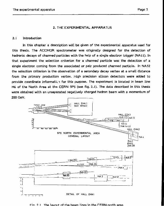
In this chapter a description will be given of the experimental apparatus used forthis thesis. The ACCMOR spectrometer was originally designed for the detection ofhadronic decays of charmed particles with the help of a single electron trigger (NA11). Inthat experiment the selection criterion for a charmed particle was the detection of asingle electron coming from the associated or pair produced charmed particle. In NA32the selection criterion is the observation of a secondary decay vertex at a small distancefrom the primary production vertex. High precision silicon detectors were added toprovide coordinate informatici for this purpose. The experiment is located in beam lineH6 of the North Area at the CERN SPS (see fig. 2.1). The data described in this thesiswere obtained with an unseparated negatively charged hadron beam with a momentum of200 GeV.
T4HGET ZONECCC 2)
HALL ECN3NA10
50 tOO 150 200 2Sff
SPS NORTH EXPERIMENTAL AREAGENERAL LAYOUT -..tNA4
[NA2JNA9[NA28
(NA20)
' M'TESl
. .—
::iNA30
(NA31)
31 NA3 '
~ L J
fNAl_ J -.
NA12 1
1 DETAIL OF HALL EHN1
Fin 9 I The lax/niih nf Khfi hetam lines in the CERN nnrfch area.
The experimental apparatus Page 4
BB T M1 0C2 M2 DC3A C3 DC3B
beam
1m
1m
DC3C
X
VMSD
BC1 BC2 BC3 BC4 AT MC1 MC2 1 2 3 <. 5 6 7
2 mm
10mm
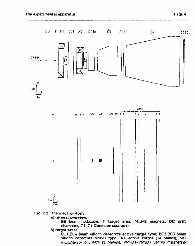
Fig. 2.2 The spectrometer:a) general overview:
BB beam hodocope, T target area, M1.M2 magnets, DC driftchambers, C1-C4 Cerenkov counters;
b) target area:BC1,BC4 beam silicon detectors active target type, BC2.BC3 beamsilicon detectors VMSD type, AT active target (14 planes), MCmultiplicity counters (2 planes), VMSD1-VMSD7 vertex microstrip
The experimental apparatus Page 5
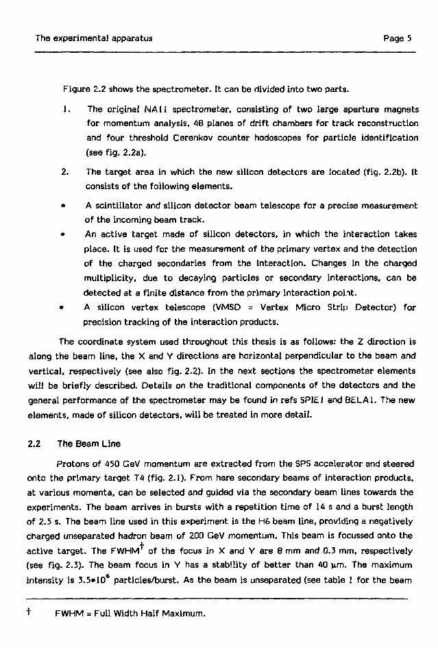
Figure 2.2 shows the spectrometer. It can be divided into two parts.
1. The original NA11 spectrometer, consisting of two large aperture magnetsfor momentum analysis, 48 planes of drift chambers for track reconstructionand four threshold Cerenkov counter hodoscopes for particle identification(see fig. 2.2a).
2. The target area in which the new silicon detectors are located (fig. 2.2b). Itconsists of the following elements.
• A scintillator and silicon detector beam telescope for a precise measurementof the incoming beam track.
• An active target made of silicon detectors, in which the interaction takesplace. It is used for the measurement of the primary vertex and the detectionof the charged secondaries from the interaction. Changes in the chargedmultiplicity, due to decaying particles or secondary interactions, can bedetected at a finite distance from the primary interaction point.
• A silicon vertex telescope (VMSD = Vertex Micro Strip Detector) forprecision tracking of the interaction products.
The coordinate system used throughout this thesis is as follows: the Z direction is
along the beam line, the X and Y directions are horizontal perpendicular to the beam and
vertical, respectively (see also fig. 2.2). In the next sections the spectrometer elements
will be briefly described. Details on the traditional components of the detectors and the
general performance of the spectrometer may be found in refs SPIE1 and BELA1. The new
elements, made of silicon detectors, will be treated in more detail.
2.2 The Beam Line
Protons of 450 GeV momentum are extracted from the SPS accelerator and steeredonto the primary target T4 (fig. 2.1). From here secondary beams of interaction products,at various momenta, can be selected and guided via the secondary beam lines towards theexperiments. The beam arrives in bursts with a repetition time of 14 s and a burst lengthof 2.5 s. The beam line used in this experiment is the H6 beam line, providing a negativelycharged unseparated hadron beam of 200 GeV momentum. This beam is focussed onto theactive target. The FWHM of the focus in X and Y are 8 mm and 0.3 mm, respectively(see fig. 2.3). The beam focus in Y has a stability of better than 40 um. The maximumintensity is 3.5*10* particles/burst. As the beam is unseparated (see table 1 for the beam
t FWHM = Full Width Half Maximum.
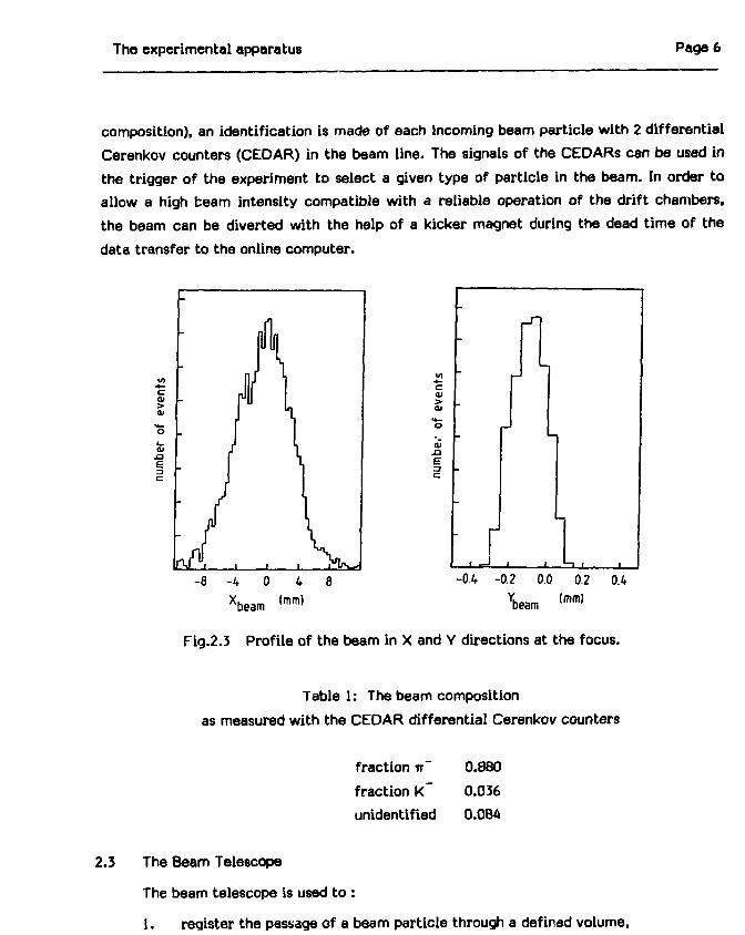
The experimental apparatus Page 6
composition), an identification is made of each incoming beam particle with 2 differential
Cerenkov counters (CEDAR) in the beam line. The signals of the CEDARs can be used in
the trigger of the experiment to select a given type of particle in the beam. In order to
allow a high beam intensity compatible with a reliable operation of the drift chambers,
the beam can be diverted with the help of a kicker magnet during the dead time of the
data transfer to the online computer.
c
>at
o
ouX )E
a
ri
rbeam (mm)
-0.4 -0.2 0.0 0.2 0.UYbeam
Fig.2.3 Profile of the beam in X and Y directions at the focus.
Table 1: The beam composition
as measured with the CEDAR differential Cerenkov counters
fraction ir~ 0.880
fraction K~ 0.036
unidentified 0.084
2.3 The Beam Telescope
The beam telescope is used to :
1. register the passage of a beam particle through a defined volume,
The experimental apparatus Page 7
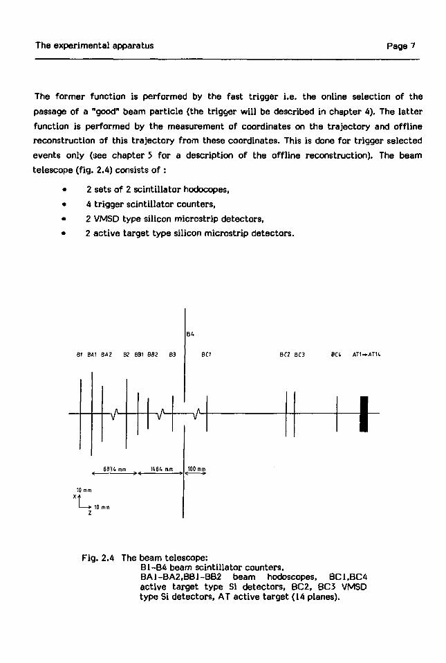
The former function is performed by the fast trigger i.e. the online selection of thepassage of a "good" beam particle (the trigger will be described in chapter 4). The latterfunction is performed by the measurement of coordinates on the trajectory and offlinereconstruction of this trajectory from these coordinates. This is done for trigger selectedevents only (see chapter 5 for a description of the offline reconstruction). The beamtelescope (fig. 2.4) consists of :
• 2 sets of 2 scintillator hodocopes,
• 4 trigger scintillator counters,• 2 VMSD type silicon microstrip detectors,• 2 active target type silicon microstrip detectors.
81 BA1 BA2 B2 BB1 BB2 B3
B4
BC1 BC2 BC3 BCU AT1-ATK
J /"
683C mm 1404 mm
10 mm
10 mm
\
100 mm
Fig. 2.4 The beam telescope:B1-B4 beam scintillator counters,BA1-3A2.BB1-BB2 beam hodoscopes, BC1.BC4active target type Si detectors, BC2, BC3 VMSDtype Si detectors, AT active target (14 planes).
The experimental apparatus Page 8
All detectors except the VMSO's can be used in the fast trigger, whereas the scintillatorcounters are omitted in the offline reconstruction. The main properties of the beamtelescope detectors are summarized in table 2.
Table 2: The elements of the beam telescope.
scintillator hodoscopes
strip orientation (°)
active area (XxYXmma)
# stripsstrip width (mm)strip distance (mm)resolution (mm)
scintillator counters
active area (XxYXmm2)
hole size (XxYXmm2)
silicon microstrip detectors
# planesorientation (°)
active area (XxYXmm2)# strips/plane
strip pitch (vim)
readout pitch(um)
resolution(um)
Angle with the horizontal.
BA1
0.
72.x48.12
6.
2.
2.AH2
Bl
60.X60.
VMSD type2
± 14.
36.X9.4
120
20.
60.
4.5
BA2
90.
48.X72.12
6.
2.
2.AT12
B2
60.X60.
BB1
0
36.X25.12
3.
1.
1./V12
B3
30.X10.
active
30
BB2
90.
25.x36.12
3.
1.
1./V12
B4
200.X200.
20.X2.
target type
2
0.
.xO.96
48
20.
20.
2.8
2.4 The Active TargetThe active target (fig. 2.5) is an array of 14 identical silicon microstrip detectors
closely packed together, followed at a distance of 40 mm by 2 large silicon microstrip
detectors, the multiplicity counters. The functions of the active target are the following :

The experimental apparatus Page 9
The first plane is used to register the beam and to veto upstream inter-
actions. The hit information is employed in the fast trigger for the selection
of a useful passage of a beam particle and to veto upstream interactions. The
pulse height information from this detector is used in the offline beam recon-
struction.
The 2 to 7 plane serve as target. A trigger on pulse height information
selects interactions in these planes (see section 4.1). The extrapolated beam
position and the knowledge of the plane in which the interaction takes place
thus define the interaction point. The six planes provide an interaction rate
which is sufficient to saturate the readout system.
The planes behind the interaction plane and the multiplicity counters record
the energy deposition by the charged secondaries of the interaction. The
pulse height information of these detectors is used to detect changes in the
charged particle multiplicity, which may be dus to e.g. decaying particles or
interactions of secondaries with the detector material.
multiplicitycounters
active target
BC4
Fig. 2.5 Active target.Isometric view of the active target with the lastbeam detector (BC4) and the multiplicity counters.

The experimental apparatus Page 1C
The main characteristics of the target may be found in table 3. A more detaile
description of the principle of operation and the performance wil l be given in chapter 3.
Table 3: The active target
# planes
active area (XxYXmm2)
thickness detector (um)
dist. between det. centres (um)
# strips/det.
strip pitch (um)
resolution (um)
strip orientation (with horizontalX")
target14
30.x0.96
280.
500.
48
20.
2.8
0.
multiplicity counters2
36.X9.6
280.
1000.
24
400.
400./V12
0.
2.5 The Vertex Microstrip Detectors.
The measurement of high precision coordinates of the secondary tracks for vertex
reconstruction is performed by the vertex microstrip detectors (fig. 2.2b). The strip pitch
of these detectors is 20 um. Only every 3 strip is read out in the inner area, and every
6 strip in the outer area. The signals on the non-readout strips are measured with the
readout strips by capacitive coupling (capacitive charge division). This readout technique
reduces the number of electronic channels with a factor 5. The spatial resolution of the
detectors for a well separated track (in the 60 um readout region) is 4.5 um. The
resolution degrades sharply when the distance between 2 tracks becomes less than 120 um
(see also section 3.5). The main characteristics of the detectors are displayed in table 4.
In chapter 3 the general principle of operation of microstrip detectors wil l be described.
More details on the detector construction and operation may be found in refs. BELA1 and
BAIL1.

The experimental apparatus Page 11
Table 4: The vertex microstrip detectors
strip orientation (°)# planes
active area (XxY)(mma)
# strips/plane
strip pitch (p.m)
# readout strips/plane
readout strip pitch
inner(outer) region (vim)
area inner region(XxYXmm2)
resolution inner(outer) region (um)
+14.3
36.X24.
1200
20.
240
60.(120.)
36.X7.2
4.5(7.8)
-14.3
36.X24.
1200
20.
240
60.(120.)
36.X7.2
4.5(7.8)
0.1
36.X24.
1200
20.
240
60.(120.)
36.X7.2
4.5(7.8)
Angle with the horizontal.
2.6 The Downstream Spectrometer.
The momentum analysis and particle identification of charged interaction products
are performed by the downstream spectrometer (fig. 2.2). To combine a good acceptance
for low momentum particles with a high momentum resolution for high momentum
particles a two magnet setup is used. Charged particles produced in the target are
deflected by a low field wide gap magnet which deflects the particles in the X-Z plane.
Their tracks are measured by the drift chambers between the two magnets (ARM2). High
momentum (2 3. GeV) forward tracks are further analyzed by a high field smaller gap
magnet (BBC). These are measured by the 3 packs of drift chambers behind the BBC
magnet (ARM3). In table 5 the momentum resolution for the different track topologies is
listed. Particle identification is provided by four threshold Cerenkov counter hodoscopes.
Hodoscope Cl is positioned in the MNP magnet, hodoscope C2 in the BBC magnet, and C3
and C4 are located downstream of the BBC magnet. Table 6 contains the most important
parameters of the spectrometer. Figure 2.6 schematically depicts the momentum windows
for particle identification.

The experimental apparatus Page 12
n
K/p
3.6 12.7
K p
1 h
24.2
I2.5 8.8 16.7
I [6.3 22.2 42.3
P
TC/K
1 1 \-
TC/K/p
1
C1
C2
C3
13.4 47.2
1 1
89.8
1 1 1 150
p (GeV)100
Fig. 2.6 Windows for particle identification.For each Cerenkov counter hodoscope the 3 momentumthreshold values are indicated, from left to right pion,kaon and proton (the numbers under the arrows). The toppart of the picture displays the momentum intervals inwhich particles can be identified, when they traverse thecomplete spectrometer. Particles which can beseparated uniquely are indicated on the top line,confused particles on the second.

The experimental apparatus Page 13
Table 5: Momentum resolutions
reconstructed inVMSD
no
no
yes
yes
no
yes
ARM2
yes
no
yes
no
yes
yes
ARM3
no
yes
no
yes
yes
yes
Ap/pin %
0.15
0.13
0.15
0.11
0.10
0.09
fraction ofall tracks
0.136
0.037
0.332
0.039
0.062
0.394
Table 6: The spectrometer
The spectrometer magnets
magnetic length (m)
window (XxY)(m2)
field integral JBydZ (Tm)
The drift chambers
# planes
active area (XxY)(m2)
wire orient. (°)
# sense wires/plane
max drift length (mm)
mean drif t velocity (um'rs)
resolution (mm)
MNP
1.3
2.4x0.6
0.90
ARM2
20
3.8x1.4
0.. ± 14.
96
20.
52.
0.17
BBC
1.7
1.6x0.5
2.06
ARM3A
16
2.0x0.8
0.. ± 30.
48
20.
52.
0.17
ARM3B
8
3.5x0.85
0.. ± 27.
94,72
20.
52.
0.17
ARM3C
2
4.5x2.
0., ± 13.5
112
20.
52.
0.17
Angles with the vertical
Cerenkov counter hodoscopes
# mirrors
threshold ir
(GeV) K
P# photoelectrons
fo ra 3=1. particle
Cl
4x14
3.6
12.7
24.2
10.
C2
2x9
2.5
8.8
16.7
15.
C3
2x11
6.3
22.2
42.3
12.
C4
2x10
13.4
47.2
89.8
9.5

Page 14

Silicon microstrip detectors Page 15
3. SILICON MICROSTRIP DETECTORS
3.1 Basic Operation
All Si microstrip detectors employed in this experiment have the same basicoperation, but can feature different readout techniques (section 3.5). Figure 3.1 showsschematically a Si microstrip detector. The detector consists of a chip of n doped highresistivity Si with electrodes on both sides. One electrode has a strip structure andconsists of p implanted regions covered with aluminium. These p implanted regions formthe strip shaped diodes which determine the operation of the detector. The otherelectrode, the so-called "back" side, consists of an n+ implanted layer, covered withaluminium. A voltage is applied between the strip electrodes and the back side in the so-called reverse bias direction. (The back side is then on positive voltage.) This voltagedepletes the counter of its free charge carriers, leaving behind the ionized dopand atomswhich produce an electric field decreasing linearly with the distance to the strips. Themaximum depletion is reached at a voltage of 120 V, the operating voltage of thesecounters. When a charged relativistic particle traverses a detector it will ionize atomsalong its path. Subsequently, the electrons from this primary ionization will ionize otheratoms. This cascade process continues until no electron has enough energy left to produceany further ionization. This means that the ionization process stops when the electronsare all left in the conduction band, each leaving behind a hole in the valence band. Theaverage energy required to produce an electron-hole pair in Si is 3.6 eV. In 280 v-m thickSi detectors the average number of electron-hole pairs so created is 24000. They areinitially located in a narrow tube around the particle trajectory. Under the influence ofthe electrical field the electrons will drift towards the "back" side and the holes to the"front" side where they will be collected at the strips. The following paragraphs deal with
particletrajectory
I i I .-1pm Aluminium
rmJ-*mf-*^*m^mr*mL->m^m-r--Q.2lim SJQ2/"-p*-Implantation(B)
E / 1^ | Si-crystaltn-type)
- n*_ Implantation (As )• 1 jjm Aluminium
Fig. 3.1 Cross section of a Si microstrip detector.
Silicon microstrip detectors Page 16
a more detailed description of several important subprocesses in Si detectors. Further
descriptions may be found in references CHAR1, HEIJ1 and RANC1.
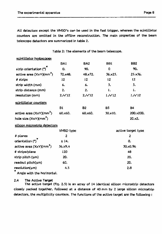
1.0 2.0pulse height (m.i.p)
Fig. 3.2 A Landau energy loss distribution.
3.2 Ionization in Si
The energy loss distribution of relativistic charged particles in matter was first
successfully described by Landau (LAND1). Vavilov refined this description (VAVI1), but
for 280 um Si both are practically identical and we will use the former. The Landau
distribution (see refs. ROSSI and KOLB1 and fig. 3.2) is based on Rutherford scattering on
free electrons. A later addition (BLUNi, SHULI) takes into account that the electrons in
matter are not free but bound. This results in a distribution which can be expressed as a
convolution of a Landau and Gaussian distribution. Thus (HANC1, HANC2):
f(A,x) = (L/avr(2ir)) ^ j " fi(A',x)exp[-(A-At)a/2o2]dA' (3.1),
with:
fi(A',x) the Landau distribution,
A the actual energy loss,
x the traversed distance in the Si,
p the density of the Si.
The width of the Gaussian distribution is given by :a2 = (8/3) IEjl.(Z./Z)ln[2mec
a|32/li]in which :
I = 153.4 (z2/3a) (Z/A)xp (keV)
(3.2).
(3.3).
Silicon microstrip detectors Page 17
with :
1, the ionization potential of the i-th shell in Si,
Z. the number of electrons in the i-th shell in Si,
z the charge of the incident particle,
Z.A the charge and atomic weight of Si.
The most probable energy loss is expressed by the Bethe-Bloch formula (FANO1):
with :
A' = x (FZpz2/A32) (ln[2m Y232c2/I]-32) (3.4),6
rn the electron mass,e
I the binding energy of electrons in Si,F = 0.307 MeV cma/g.
Not taken into account are very energetic 6-rays which can escape out of the thin
detectors, thus reducing the tail of the distribution. A measured distribution will also
include noise which is due to two sources : the intrinsic detector noise, and the electronics
noise. When expressing a measured distribution in terms of the above formalism, the width
of the contributing Gaussian wil l be :
aGauss = ^°' + °* int. noise + a%lec. noise] (3-5)-
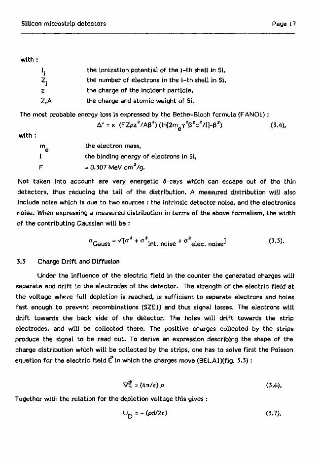
3.3 Charge Dri f t and Diffusion
Under the influence of the electric field in the counter the generated charges wil l
separate and drift to the electrodes of the detector. The strength of the electric field at
the voltage where full depletion is reached, is sufficient to separate electrons and holes
fast enough to prevent recombinations (SZEi) and thus signal losses. The electrons wil l
drift towards the back side of the detector. The holes wil l drift towards the strip
electrodes, and wil l be collected there. The positive charges collected by the strips
produce the signal to be read out. To derive an expression describing the shape of the
charge distribution which will be collected by the strips, one has to solve first the Poisson
equation for the electric field E in which the charges move (BELAl)(fig. 3.3):
V? = (4n/e) p (3.6),
Together with the relation for the depletion voltage this gives :
U D = - (pd/2e) (3.7).

Silicon microstrip detectors Page 18
particletrajectory
withd
P
Fig. 3.3 Definition of symbols in the drift calculation.a) Schematic representation of a Si microstrip
detector,b) electric field E in a detector,c) charge distribution (expression 3.13).
the thickness of the counter,
the charge density of dopand ions,
the voltage at which full depietion is reached,the dielectric constant.
This gives for the electric field as function of the depth z in the detector :
£ = (0.0.E)
withUC
ud
E(z) = ((U-UD)/d) + (2UDz/d*
the voltage at which full depletion is reached,the applied voltage,the detector thickness.
The drift velocity is then given by :v = (dz/dt) = uE(z)
with :V- the mobility of the holes.
(3.8).
(3.9).

Silicon microstrip detectors Page 19
10- 7
i o - 8 t .
— - « - 9
1 0 - 1 0
40 80 120 160 200 240 280
Z (U.ID)
40 80 120 160 200 240 280
z
Fig. 3.4 a) Drift time of holes as function of the drift distancein a Si microstrip detector with U = UQ- = -120 V(expression 3.10);
b) Width of the charge cloud after drift to the strips asfunction of the drift distance (expression 3.12).
Integration of (3.9) will then provide us with the relation between the drift time and the
drift distance (fig. 3.4a):
t(z) = (-da/2nUD) ln[l - (2UD(d-z)/(U-UD)d)] (3.10),During this drift process, the charge cloud will disperse due to diffusion. In the absence ofan electric field and recombination of electrons and holes, the charge distribution as aresult of diffusion will be :
with : D.
c(x.y.t) = (l/4nDht) exp[- (x +y )/4Dht] , 0Sz<d
the transverse diffusion constant of holes In Si,
(3.11).

Silicon microstrip detectors Page 20
Integration over x gives the charge distribution in the projection perpendicular to thestrips :
c(y.fc) = _ „ / " c(x.y.t)dx = (l/^(4nDht)d) exp[- (y2/4dht)] (3.12).
We can now include the effect of the finite width of the initial charge distribution 6 byreplacing the time t by t+to with to = 62/2D. (fig. 3.4b). The effect of the electric field isexpressed by the relation between t and z (expression 3.10). Integration over z will thenproduce the charge distribution at the strips.
f(y) = (lAr(4nDh)d) Jd (dz/(^(t+to)) exp[-(y2/4dh(t+to))] (3.13).
The charge distribution after drifting to the strips is thus an integral over Gaussiandistributions. The width of the distributions increases with the drift distance. For a trackincident at right angles the Gaussians are centered around the same position, resulting ina symmetric charge distribution. For tracks incident at other angles the Gaussians will notbe centered around the same position, resulting in an asymmetric charge distribution.
3.4 Charge Deposition by Inelastic Interactions
In an interaction of high energy particles with a Si nucleus in the detector, thelarge ionization observed will be due to more than just the ionization of the incomingparticle before the interaction and the produced particles after the interaction. In theinteraction the nucleus itself may be excited and send out fragments. The nucleus mayalso recoil and then lose its energy via ionization. This can produce large chargedepositions in the target detector. The inelastic interactions in Si can be divided into 3categories (RANC1).
• Coherent interactions. All 28 nucleons of the Si nucleus participate in the
interaction. The nucleus recoils but remains in the ground state.
• Semicoherent interactions. The nucleus recoils and is internally only
disturbed to the extent that it is left in a well defined state.
e.g.: h+ aeSi->h* 2eSi* (1.78 MeV)'-»Y+ 28Si.
• Incoherent interactions. The interaction takes place with one or morenucleons. The nucleus is left behind in an excited state.

Silicon microstrip detectors Page 21
In all 3 cases the end products contain a number of secondary particles and a
recoiling nucleus. This recoil produces, depending on its energy, a rather large amount of
ionization. In the case of excitation, the nucleus can send out ("evaporate") nucleons or
groups of nucleons. At the energies involved (« 1 GeV) these particles are also highly
ionizing. Apart from coherent interactions with a small recoil, all interactions will
produce a significant amount of ionization. This fingerprint of an inelastic interaction can
be used to locate an interaction in the active target. This can be used for two purposes :
online to trigger on interactions and offline to reject interactions of secondaries in the
planes downstream of the primary interaction vertex. Figure 3.5 shows an example of an
interaction in tHfe target.
detector plane
.a£
123456789IB11121314
IBIE171819282122232425262728 •2338313233343536373839
4142434445464748
1 2 3 4 S
s56
46335787777718613
4 6* 9» 7****<9. 9 B i
3
B626383
**»
42444BSBS758SI4948128BG7
e
3
3
42272S356G947479
3
18323741495858
7
162325331146
8
4
5
1119B837IB7
11\2
9
141163
31119E47
18
414183
9
2751444
12
11
71857
4
211318734
378
6B
12
BS49
7
2718
18
455
318B
13
113
S
7
1118
4
43
11
14
5
4IB
9
36
113
363
7
22
4
Fig. 3.5 Example of an interaction in the active target. Thecolumns depict the detectors, the rows depict the strips.The ADC pulse heights are given in units of 0.1 mini-mum ionizing particles. An overflow is indicated as *** .The interaction vertex is pointed out by the symbol <.The fitted incident beam track is indicated with a *.
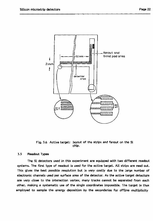
Silicon microstrip detectors Page 22
fanout andbond pad area
Fig. 3.6 Active target: layout of the strips and fanout on the Sichip.
3.5 Readout Types
The Si detectors used in this experiment are equipped with two different readoutsystems. The first type of readout is used for the active target. All strips are read out.This gives the best possible resolution but is very costly due to the large number ofelectronic channels used per surface area of the detector. As the active target detectorsare very close to the interaction vertex, many tracks cannot be separated from eachother, making a systematic use of the single coordinates impossible. The target is thusemployed to sample the energy deposition by the secondaries for offline multiplicity

Silicon microstrip detectors Page 23
analysis. To lead the signals from the 20 urn strips to the electronics a fanout isnecessary. On the chip (fig. 3.6) a fanout pattern is provided which leads from the strips,with 20 um pitch, to the bonding pads, with 180 urn pitch. The pads are connected to anexternal Kapton fanout with ultrasonically bonded wires. The connection to thepreamplifiers is made with connectors soldered on the other end of the Kapton fanouts(fig. 3.7). The second type of readout is used for the VMSD's. In the central area every
aim J mini
Fig. 3.7 Fully assembled active target module.In the centre the quartz plates onto which the detectorsare glued. The detectors are oriented alternatively toleft and right.
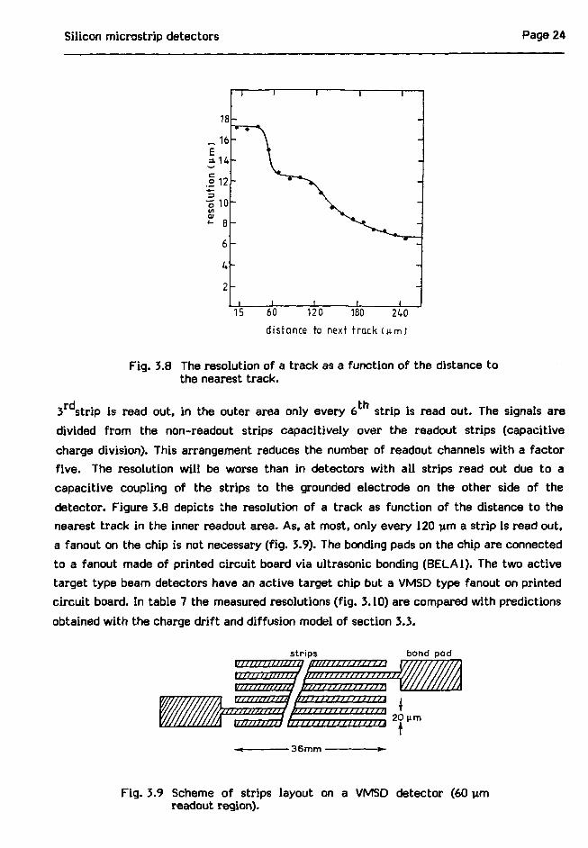
Silicon microstr ip detectors Page 24
60 120 180 240
distance to next track Cum)
Fig. 3.8 The resolution of a t rack as a funct ion of the distance tothe nearest t rack.
3 str ip is read out, in the outer area only every 6 str ip is read out. The signals are
divided f rom the non-readout strips capaci t ively over the readout strips (capacit ive
charge division). This arrangement reduces the number of readout channels w i th a fac to r
f i ve . The resolution w i l l be worse than in detectors w i th al l strips read out due to a
capacit ive coupling of the strips to the grounded electrode on the other side of the
detector. Figure 3.8 depicts the resolution of a track as funct ion of the distance to the
nearest t rack in the inner readout area. As, at most, only every 120 ixm a str ip is read out,
a fanout on the chip is not necessary ( f ig . 3.9). The bonding pads on the chip are connected
to a fanout made of pr inted c i rcu i t board via ultrasonic bonding (BELA1). The two act ive
target type beam detectors have an act ive target chip but a VMSD type fanout on pr inted
c i rcu i t board. In table 7 the measured resolutions ( f ig . 3.10) are compared w i th predictions
obtained w i t h the charge d r i f t and dif fusion model of section 3.3.
,t .,., ,,,!J1 fi/.j. ;J.//>,///> L 20 urn/} i/i/n/jiifi iiIIimi111miiTn i r
Fig. 3.9 Scheme of strips layout on a VMSD detector (60 urnreadout region).
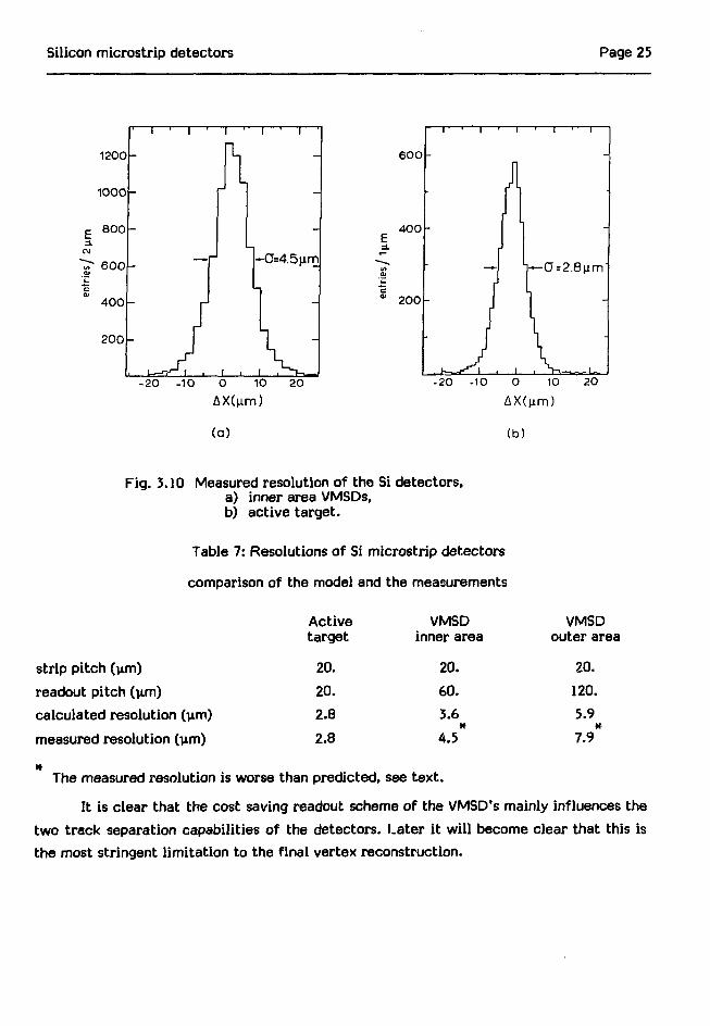
Silicon microstrip detectors Page 25
1200- 6OO -
400 -
200 -
(a)
-20 -10 O 10 20
AX(nm)
(b)
Fig. 3.10 Measured resolution of the Si detectors,a) inner area VMSDs,b) active target.
Table 7: Resolutions of Si microstrip detectors
comparison of the model and the measurements
strip pitch (y.m)
readout pitch (um)calculated resolution (vim)
measured resolution (um)
Activetarget
20.
20.
2.8
2.8
VMSDinner area
20.
60.
3.6
4.5
VMSDouter area
20.
120.
5.9
7.9
The measured resolution is worse than predicted, see text.
It is clear that the cost saving readout scheme of the VMSD's mainly influences the
two track separation capabilities of the detectors. Later it will become clear that this is
the most stringent limitation to the final vertex reconstruction.

Silicon microstrip detectors Page 26
3.6 Detector Mounting and Electronics
The microstrip detectors have resolutions of a few microns which requires a highprecision in the mounting of the detectors. The position has to be fixed in all 3 directionswithin a few urn during data taking. Furthermore the detectors have to be parallel withina few tenths of urn and the distances between the detectors have to be known with aprecision of ± 10 urn. To achieve this, the detectors are mounted on quartz precisionplates and kept at fixed distances with precision gauge blocks. This assembly is placed onan optical bench and pressed together. For the different types of detectors the mountingon the quartz plates is as follows :
Vdetector
bias col in• 120V
preamp
T
ampdriver
gainadjust
8 bitsMain A O C
detay~6Om• Comae
discrim.ECL
to trigger logic
dete
Cal in
- Camac
i Imatching
transf.
Fig. 3.11 a) Block scheme of the active target electronics,b) block scheme of the VMSD electronics.
1. Active target type beam detectors; mounted separately on 14 mm quartz plateslike the VMSD's,
2. Active target; 14 detectors each mounted on a 0.5 mm thick quartz plate andjoined together in one module (fig. 3.7),
3. The two multiplicity counters; mounted on 1 mm thick quartz plates and placedtogther in one module,
4. VMSD; mounted separately on 14 mm thick quartz plates (BELA1).

Silicon microstrip detectors Page 27
The electronics for the VMSD system is described in refs. BELA1 and BAIL1. Theactive target uses a chain of electronics similar to that of the VMSD's. The blockdiagrams are shown in fig. 3.11. The input charge from the detectors for 1 rn.i.p. is4»10~15C (24000 holes) which is amplified and shaped in steps by a preamplifier, anamplifier driver and a main amplifier to a 100 mV pulse as input for an 8-bit ADC. Gainadjustment is made with an external voltage. For triggering purposes the main amplifierdelivers in parallel a digital ECL signal via an adjustable discriminator. In total 816channels are read with this system.
minimum ionizing particle.

Page 28
The trigger, calibrations and data taking Page 29
A. THE TRIGGER, CALIBRATIONS AND DATA TAKING
4.1 The Trigger
The trigger employed in this experiment is an interaction trigger. This trigger hasthe advantage that it introduces only minimal biases. Furthermore no decay channel willbe excluded by the trigger and thus a wide range of physics possibilities remain open forthe analysis. The disadvantage of an interaction trigger is that no trigger enrichment ofgood events takes place before the events are written to tape. Thus the event selectionwill have to take place in the offline analysis.
The selection of interactions is done in two steps, the beam trigger and theinteraction trigger.
1. The beam trigger itself is in turn split up into three steps. In the first stepthe total beam flux is measured with the scintillation counters Bl and B2 (seefig. 2.4)
CONTROL = B1-B2 (4.1).In the second step a coarse beam definition is made restricting the beam intoa slit matching the size of the active target (AT) planes with a height of1 mm and a width of 30 mm. Two scintillator counters are used here: B3 andthe hole counter B4 (see fig. 2.4).
UB1 = CONTROL •B3«B4 (4.2).
In the third step the beam definition is refined with the help of the Si micro-
strip detectors BC4 and ATI (fig. 2.4). The detector ATI is employed to
select one particle passing through the central 16 strips out of 48 in ATI.
Clusters of neighbouring hits are taken here as only one hit (the so called
cluster mode). The detector BC4 antiselects upstream interactions, vetoing
events with hits in the 2 outer groups of 16 strips (out of 48 strips).
UB2 = UBl»BC4(l-16,33-48)«ATl(17-32) (4.3).Before data taking the beam shape was optimized so as to maximize the ratio
UB2/CONTROL.
2. The interaction trigger selects events which have a strip in the active targetwith a large (> 3 m.i.p.) pulse height (see section 3.4 on charge deposition byinelastic interactions). The strips used for this are the central 16 strips (out
The trigger, calibrations and data taking Page 30
of 48) of the active target planes 2 to 7. In addition, a charged particlemultiplicity of three or more is demanded in the two downstream multiplicitycounters (see fig. 2.5). This last requirement is made to exclude triggers inthe target due to very energetic 6-rays, elastic scattering and diffractiveinteractions with low multiplicity which do not contain charm. As events witha detectable charm decay contain at least two charged tracks from thedecaying particle, and very probably many more from the primary interactionor other decaying particles, a cut at three is still a very safe choice.The trigger selection works now in two steps.
The first step is the trigger on strips with a high pulse height in the activetarget planes 2-7.
INT1 = UB2» i a J - 7 ATj ( 3 \ 17-32) (4.4).
The second step adds the condition imposed on the multiplicity counters. Onemultiplicity counter plane provides a trigger demanding at least one stripwith a pulse height of i 3 m.i.p. (MCI . ), the other a trigger demanding atleast three strips with each a pulse height 2 1 m.i.p. (MC2 ^ ). These twoconditions are put in a logical OR.
INT2 = INTl«(MCl(j) + MC2^) (4.5).
From the trigger rates given in table 8 one can conclude that the interaction
trigger rate is 0.25%. Comparing this number with the expected rate (PDG1)
of 0.37%, one has to correct for the loss of cross section due to three prong
interactions (FLAM1), which are not accepted by the trigger. The expected
rate is then 0.28% yielding a trigger efficiency of 88.4%.
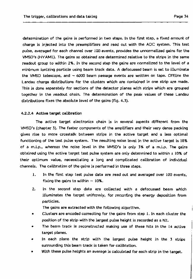
Figure 4.1 displays the distribution of the charge sum over all strips in the planesfor the interaction trigger. The peak at one m.i.p. is due to the beam particle before theinteraction vertex in any of the planes 2-7. In these planes the beam signal graduallydisappears. In these and following planes one sees the ionization due to the interactionsand the interaction products.
The negative 200 GeV H6 beam contains 3.5% kaons (table 2.1). By reducing thenumber of pion interaction triggers with respect to the number of kaon interactiontriggers, a sizable quantity of K~ induced interactions can also be recorded. Kaoninteractions (MASTER l)are detected with the interaction trigger (INT2) and the signal

The trigger, calibrations and data taking Page 31
c01
01
ZJC
plane 1
11
12
2 4 6 6 10 12 14 2 4 6 8 10 12pulse height (m.i.p.)
Fig. 4.1 The distribution of the total charge sum in the activetarget planes.The shape of the distribution is explained in the text.
from the CEDAR 1 Cerenkov counter in the beam line. All other interactions are labeled
pion interactions. The pion interaction rate is artificially reduced by a coincidence with a
random signal (MASTER2). The interaction trigger (TRIGGER) is taken as the OR between
trigger
burst gatepile up
Fig. 4.2 The trigger scheme.
CEDAR1
MC1-2

The trigger, calibrations and data taking Page 32
the kaon and pion interaction triggers. This evidently reduces the total trigger rate. For
this reason the experiment was run with the highest possible beam intensity which still
ensures a reliable drift chamber operation. With a data taking rate of 90% of the pion-
only rate, the kaon interaction rate is 30% of the total interaction rate. Figure 4.2 shows
a scheme with the complete trigger logic. In table 8 an example is given of the trigger
rates.
Table 8: Example of trigger rates taken in 41 bursts of 2.5 sec duration.
Number of triggers
CONTROL 70110488
UB1 64375601
UB2 48763884
INT2 119584
MASTER 1 3707
MAS1ER2 10766
TRIGGER 14140
TRIG to tape 6681
4.2 The Calibration of Detector and Electronics
4.2.1 Introduction
In order to transform the signals of the tracking detectors into coordinates, several
parameters of the detectors and their electronics have to be determined in advance. This
calibration is split up into two phases for all detectors. The first phase is the calibration
of the readout electronics, determining signal amplification factors and relative timing
constants. The second phase is the calibration of the geometry, in which the positions of
ail the detectors are determined. These calibrations, using test pulse and beam track data,
are performed at regular intervals during data taking.
4.2.2 The calibration of the electronics
Two types of readout electronics are employed in the apparatus. The first is a
time digitization system used for the drift chambers. The second type are Analog to
Digital Converters (ADC), which are used to measure the light production in the Cerenkov
counters and the charge deposition in the Si detectors.
The trigger, calibrations and data taking Page 33
4.2.2.1 Drift chamber calibration
The drift chambers have a time digitization system for which the relative timing
of the channels with respect to each other have to be determined (TO's). Details on the
drift chamber system and its calibrations can be found in ref. DAUM1.
4.2.2.2 Cerenkov counter calibration
From the Cerenkov ADC's the zero readings (pedestals) and the gain factors of
the photomultiplier-ADC chains have to be determined. Both are obtained from pulse
height spectra in which the pedestal and the single photon signals stand out as distinct
peaks.
4.2.2.3 The vertex microstrip detector calibration
The pedestals fo r the VMSD's are obtained by reading out empty events (no beam
on target ) . The ADC signals in these empty events are averaged fo r each channel over 100
events. For moni tor ing purposes the standard deviat ions of the pedestals are also
calcu lated and saved, as they contain the in format ion on the noise leve l . The
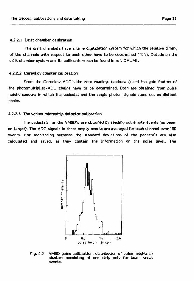
F ig . 4.3
0.8 1.6 2.4pulse height (m.i.p.)
VMSD gains ca l ib ra t ion; d is t r ibut ion of pulse heights inclusters consisting of one st r ip only f o r beam t rackevents.
The trigger, calibrations and data taking Page 34
determination of the gains is performed in two steps. In the first step, a fixed amount ofcharge is injected into the preamplifiers and read out with the ADC system. This testpulse, averaged for each channel over 100 events, provides the unnormalized gains for theVMSD's (HYAM1). The gains so obtained are determined relative to the strips in the samereadout group to within 2%. In the second step the gains are normalized to the level of aminimum ionizing particle using beam track data. A defocussed beam is set to illuminatethe VMSD telescope, and ~ 6000 beam passage events are written on tape. Offline theLandau charge distributions for the clusters which are contained in one strip are made.This is done separately for sections of the detector planes with strips which are groupedtogether in the readout chain. The determination of the peak values of these Landaudistributions fixes the absolute level of the gains (fig. 4.3).
4.2.2.4 Active target calibration
The active target electronics chain is in several aspects different from the
VMSD's (chapter 3). The faster components of the amplifiers and their very dense packing
gives rise to more crosstalk between strips in the active target and a less optimal
functioning of the test pulse system. The resulting noise level in the active target is 18%
of a m.i.p., whereas the noise level in the VMSD's is only 3% of a m.i.p. The gains
obtained using the active target test pulse system are only determined to within ± 10% of
their optimum value, necessitating a long and complicated calibration of individual
channels. The calibration of the gains is performed in three steps.
1. In the first step test pulse data are read out and averaged over 100 events,fixing the gains to within -10%.
2. In the second step data are collected with a defocussed beam whichilluminates the target uniformly, for recording the energy deposition fromparticles.The gains are extracted with the following algorithm.
• Clusters are encoded correcting for the gains from step 1. In each cluster theposition of the strip with the largest pulse height is recorded as a hit.
• The beam track is reconstructed making use of these hits in the 14 activetarget planes.
• In each plane the strip with the largest pulse height in the 3 stripssurrounding this beam track is taken for calibration.
• With these pulse heights an average is calculated for each strip in the target.

The trigger, calibrations and data taking Page 35
This method uses the feature that the Landau tail is caused mostly by
energetic 6-electrons, emitted at high angles, which have a long range and
can deposit their energy accordingly over more strips. In detectors with
20 v-m strip pitch the charge distribution loses the Landau tai l , when only the
pulse height of the strip with largest pulse height in a cluster is taken. This
method wil l result in gains ~ 20% lower than the m.i.p. level, as the
ionization due to short range electrons is in most cases shared by two strips
(fig. 4.4a).
mbe
r of
eve
nts
c
-
rr
i—
1
i
a
8 12 16 20pulse height (a.u.)
80 120 160 200pulse height (a.u.)
240
Fig. 4.4 Active target gains calibration.a) Distribution of the pulse height of the strip
with the largest pulse height around the beamtrack after correction with gains factors asfound with the test pulse system.
b) Distribution of the pulse height in a clusterafter correction for relative gains for individualstrips. The broken line represents the f i t to aLandau distribution convoluted with a Gaussiandistribution.
In step 3 the gains are normalized to the minimum ionizing particle level
using the same beam track algorithm as for step 2, but now the gains
obtained in step 2 are used. For each plane the pulse heights in the cluster
are added and subsequently the distribution of the sums of these pulse heights
is f i t ted with a Landau distribution convoluted with a Gaussian (see section
3.2). The peak value determines the normalization of the gains (fig. 4.4b).

The trigger, calibrations and data taking Page 36
4.2.3 The calibration of the geometry
The calibration of the geometry is an essential first step in the analysis. Theresolution of the tracks reconstructed as well as the track finding efficiency dependclosely on the knowledge of the exact position and orientation of the detectors. Thespatial resolution of the tracks determines the momentum resolution and the secondaryvertex resolution. The calibration consists of two phases, the optical (hardware) and thesoftware alignment.
4.2.3.1 Optical alignment
The optical alignment is the actual positioning of the detectors, which is done or
checked before each data taking run. The magnets and Cerenkov counters are aligned by
reading their positions with respect to a ruler fixed on the floor of the experimental hall.
The drift chambers are positioned perpendicular to the beam direction (X-Y plane) and
are aligned with respect to beam axis in both horizontal (X) and vertical (Y) directions.
Their longitudinal positions (Z) are determined with the help of an optical pointer system,
which is again refered to the ruler on the floor.
The target area is aligned in two steps. First the Si detectors are positioned on anoptical bench (see section 3.5), then this internally rigid assembly of bench and detectorsis positioned with respect to the rest of the spectrometer. The errors on the positions ofall components (the target table is seen here as one component) is ~ 1 mm.
4.2.3.2 Software alignment
The second phase in the calibration is the software alignment in which thepositions obtained with the optical alignment are fine tuned. Using coordinates obtainedwith the nominal positions of the detectors as found in step one, tracks are fitted in thedetectors, leaving out detectors successively. The distances of single coordinates to thisfitted track are plotted for each detector. The peak positions of these residuals'distributions are used to redefine the positions of the detectors. This procedure isrepeated several times to obtain the optimal position. For the drift chamber system thisprocedure has been extensively described in refs. SPIE1 and PETE1. After the driftchambers have been aligned, the silicon detectors on the target table are adjusted withrespect to the drift chamber system.

The trigger, calibrations and data taking Page 37
This software fine tuning can only be done in directions perpendicular to the beamaxis. The Z-positions obtained in the hardware phase are not changed. The alignmentquality can be monitored from the distributions of the residuals from the tracks fitted atthe end of the procedure. Figure 4.5a shows a typical distribution of residuals for the driftchambers. The alignment of these chambers can be performed with a precision of 40 urn.Figure 4.5b shows a distribution of residuals for a VMSD detector. The precision here is4.0 um.
1/1
even
l
o
num
ber
-
_J
a
CD- QEC
m
J
I b
- 2 - 1 0 1Ax (mm)
-0.03 -0.02 -0.01 0.0 001(mm)
0.02 003
Fig. 4.5 Calibration of the geometry.a) Distribution of residuals of drift chamber co-
ordinates with respect to a beam track fittedwith the other drift chambers.
b) Distribution of residuals of VMSD detector co-ordinates with respect to a beam track fittedwith the other VMSD's.
4.3 Data Taking and Data Sample
The events passing the trigger are read out via CAMAC into the NORD 100 data
acquisition computer and written onto tape. The data acquisition rate is ~ 160 events
written to tape per burst of 2.5 s. At this speed a 6250 bpi tape is full in 35 minutes. The
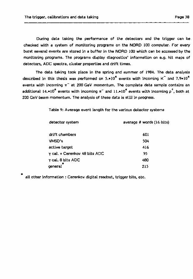
average readout time per event is 15 ms. Table 9 shows a breakdown of the averaged
event length for the various detector systems.
The trigger, calibrations and data taking Page 38
During data taking the performance of the detectors and the trigger can be
checked with a system of monitoring programs on the NORO 100 computer. For every
burst several events are stored in a buffer in the NORD 100 which can be accessed by the
monitoring programs. The programs display diagnostics' information on e.g. hit maps of
detectors, ADC spectra, cluster properties and drift times.
The data taking took place in the spring and summer of 1984. The data analysis
described in this thesis was performed on 5.»10* events with incoming K~ and 7.9»10*
events with incoming IT" at 200 GeV momentum. The complete data sample contains an
additional 14.»10* events with incoming IT" and l l .»10* events with incoming p , both at
200 GeV beam momentum. The analysis of these data is stil l in progress.
Table 9: Average event length for the various detector systems
detector system average # words (16 bits)
drift chambers 601
VMSD's 504
active target 416
Y cal. + Cerenkov 48 bits ADC 95
Y cal. 8 bits ADC 480
general 215
*all other information : Cerenkov digital readout, trigger bits, etc.

Track reconstruction and event selection Page 39
5. TRACK RECONSTRUCTION AND EVENT SELECTION
5.1 Introduction
The offline event reconstruction comprises track reconstruction in Si detectors anddrift chambers, particle identification with the Cerenkov counter hodoscopes and secon-dary vertex reconstruction with the tracks. The average time used for the full recon-struction of an event is ~ 4 s/event (IBM 370/168 equivalent time). To reduce this workload, the event reconstruction is split up into steps; these steps include selection criteria.When events fail these criteria, they are rejected for further reconstruction. In this way,a work load reduction is achieved, as the rejected events do not require any furtherattention. Figure 5.1 schematically depicts the reconstruction and selection steps whichare also listed below.
1. Decoding of the raw data into physical quantities.
2. Reconstruction of the incoming beam trajectory in the beam telescope.
3. Reconstruction of the primary interaction vertex in the active target.
4. Preselection. Tracks are reconstructed in the vertex telescopes in projec-
tions. Events are selected which have at least 2 tracks in projections which
do not point back to the primary interaction vertex.
5. Drift chamber track reconstruction. Using DC coordinates, track segmentsare reconstructed in the arms of the spectrometer. These track segments arematched to each other. A momentum measurement of the track is obtainedwith a fitting procedure.
6. Particle identification. Using the drift chamber tracks and their momenta,the Cerenkov counter information is employed to assign a particle probability(pion, kaon or proton) to the track.
7. Microtrack reconstruction. With the drift chamber tracks as a guide, tracksare reconstructed in the vertex telescope using the coordinates from the Simicrostrip detector's.
8. Secondary vertex reconstruction. A secondary vertex search is done with thetracks as found in the vertex telescope. The search is restricted to thosetracks which form an invariant mass in a window around the charm region.
In the following sections these steps will be described in more detail.

Track reconstruction and event selection Page 40
decoding
beam track search
interaction point search
L
preselection —> no, reject event
yes
track searchdrift chambers ARM 3
Lguided track search
drift chambers ARM 2
Lopen track search
drift chambers ARM 2
drift chamber track match
global f i t drift chamber tracks
drift chamber guidedmicro track search
vertex/drift chamber guidedmicro track search
particleidentification
global fit of micro str ip/drift chamber tracks
secondary vertex search
Fig. 5.1 The reconstruction and selection steps in the analysis.
Track reconstruction and event selection Page 41
5.2 Decoding of the Raw Data
Before track reconstruction can be started, the raw data have to be decoded into
physical quantities like coordinates, quantities of charge or number of photoelectrons. For
most detectors like drift chambers and Cerenkov counters these procedures have been
described elsewhere (DAUM1, SPIE1). For the Si microstrip detectors, the procedure is
complicated by the high track density near the vertex which may cause overlaps in the
charge clouds deposited by adjacent tracks. We shall therefore describe the decoding
procedure for the Si detectors here in some detail. The coordinate attribution for the Si
detectors is done in three steps.
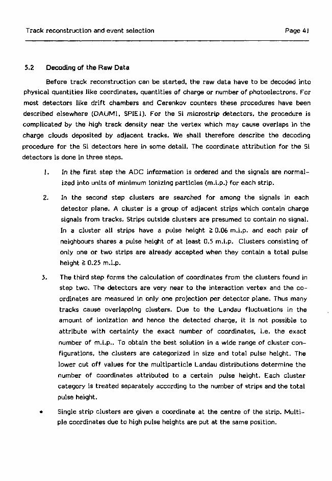
1. In the first step the ADC information is ordered and the signals are normal-
ized into units of minimum ionizing particles (m.i.p.) for each strip.
2. In the second step clusters are searched for among the signals in each
detector plane. A cluster is a group of adjacent strips which contain charge
signals from tracks. Strips outside clusters are presumed to contain no signal.
In a cluster all strips have a pulse height £ 0.06 m.i.p. and each pair of
neighbours shares a pulse height of at least 0.5 m.i.p. Clusters consisting of
only one or two strips are already accepted when they contain a total pulse
height § 0.25 m.i.p.
3. The third step forms the calculation of coordinates from the clusters found in
step two. The detectors are very near to the interaction vertex and the co-
ordinates are measured in only one projection per detector plane. Thus many
tracks cause overlapping clusters. Due to the Landau fluctuations in the
amount of ionization and hence the detected charge, it is not possible to
attribute with certainty the exact number of coordinates, i.e. the exact
number of m.i.p.. To obtain the best solution in a wide range of cluster con-
figurations, the clusters are categorized in size and total pulse height. The
lower cut off values for the multiparticle Landau distributions determine the
number of coordinates attributed to a certain pulse height. Each cluster
category is treated separately according to the number of strips and the total
pulse height.
• Single strip clusters are given a coordinate at the centre of the strip. Multi-
ple coordinates due to high pulse heights are put at the same position.

Track reconstruction and event selection Page 42
• In two and three strip clusters the coordinates are determined with a "centreof gravity" method. This is done after an attempt to cut the cluster down to atwo strip cluster by removing an outer strip with a pulse height smaller than0.2 m.i.p. If in both outer strips the signals are smaller than 0.2 m.i.p. weretain the strip with the larger pulse height.
• For clusters over 4 strips or more, we try to make a split into subclusters.Strips with a pulse height lower than 0.2 m.i.p. are taken as subclusterboundary. The subclusters of one, two and three strips are treated in a similarway as above. In the remaining 4 and more strip (sub)clusters the coordinatesare evenly divided such that, at each interstrip gap, at least one coordinate isattri- buted. The number of coordinates attributed to each interstrip gapdepends on the sum of pulse heights in the two surrounding strips.
The errors to be assigned to the coordinates are determined in an empirical
way. We search for and fit tracks (see section 5.8), leaving out each detector
plane in turn. The distance of the track to the selected coordinate in this
detector plane is plotted. This is done separately for each category of co-
ordinates. The standard deviations of these distributions are taken as errors
on the coordinates. The shape of these distributions also provide a check
whether the choice of the categories was correctly done (see fig. 5.2).
5.3 The Reconstruction of the Beam Trajectory
The incoming beam trajectory is registered by the detectors of the beam telescopeand the active target (figs. 2.4 and 2.5). Offline this trajectory is reconstructed, using thecoordinates as provided by the decoding routines. The reconstructed beam trajectory(from now on called beam track) will later on be used to find the interaction vertex in theactive target. The beam track alone will determine the X,Y coordinates of this inter-action vertex. Before describing the reconstruction algorithm, it is useful to reiterate thestrip orientation of the beam detectors and the active target planes (see figs. 2.4 and 2.5and tables 2 and 3 in chapter 2).
• BC1 and BC4 are active target type detectors with horizontal strips.• BC2 and BC3 are VMSD type detectors with strips at ±14° with the hori-
zontal.
• The beam hodoscopes BB1 and BB2 have horizontal and vertical strips res-pectively.
• The active target has horizontal strips.

Track reconstruction and event selection Page 43
-2 0AM.
-2 0ML
Fig. 5.2 Distributions of the deviations of predicted and meas-ured coordinates normalized to the errors for 4 types ofclusters in the 60 um readout regions, a) one strip, onem.i.p., b) two strips, one m.i.p., c) two strips, twom.i.p., d) three strips, two m.i.p.
The reconstruction is done as follows. Coordinates are first selected in the detec-
tors of the beam telescope and subsequently used in a track f i t . The minimum set of coor-
dinates required for a track f i t are two X coordinates and two Y coordinates. When more
coordinates are available, they will also be selected. The detectors BC2 and BC3 are each
required to supply one coordinate, giving effectively one X,Y pair. Plane BC4 and the first
four planes of the active target have to supply together one Y coordinate. In these 5 de-
tectors the Y coordinate with the best resolution is selected for the f i t . The additional X
coordinate is obtained either from the beam hodoscope BB2 or, when no hits are present
there, from the extrapolation of the X obtained with BC2 and BC3 assuming a track slope
Track reconstruction and event selection Page 44
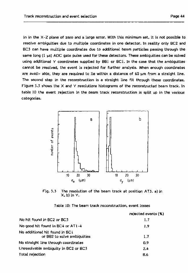
in in the X-Z plane of zero and a large error. With this minimum set, it is not possible toresolve ambiguities due to multiple coordinates in one detector. In reality only 8C2 andBC3 can have multiple coordinates due to additional beam particles passing through thesame long (1 vis) ADC gate pulse used for these detectors. These ambiguities can be solvedusing additional Y coordinates supplied by BB1 or BC1. In the case that the ambiguitiescannot be resolved, the event is rejected for further analysis. When enough coordinatesare avail- able, they are required to lie within a distance of 60 um from a straight line.The second step in the reconstruction is a straight line fit through these coordinates.Figure 5.3 shows the X and Y resolutions histograms of the reconstructed beam track. Intable 10 the event rejection in the beam track reconstruction is split up in the variouscategories.
c01
JO
e
,110 20 30
ay ((ifn)
Fig. 5.3 The resolution of the beam track at position AT3. a) inX, b) in Y.
Table 10: The beam track reconstruction, event losses
No hit found in BC2 or BC3
No good hit found in BC4 or AT 1-4
No additional hit found in BC1or BB2 to solve ambiguities
No straight line through coordinatesUnresolvable ambiguity in BC2 or BC3Total rejection
rejected events (%)
1.7
1.9
1.70.92.48.6
Track reconstruction and event selection Page 45
5.4 The Reconstruction of the Primary Interaction Vertex
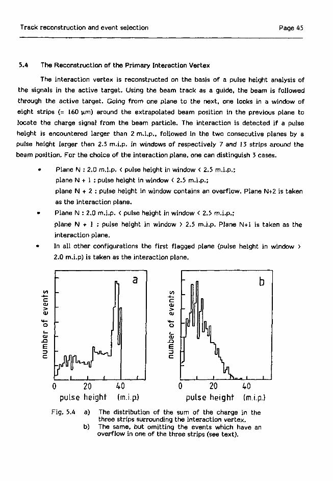
The interaction vertex is reconstructed on the basis of a pulse height analysis of
the signals in the active target. Using the beam track as a guide, the beam is followed
through the active target. Going from one plane to the next, one looks in a window of
eight strips (= 160 jim) around the extrapolated beam position in the previous plane to
locate the charge signal from the beam particle. The interaction is detected if a pulse
height is encountered larger than 2 m.i.p., followed in the two consecutive planes by a
pulse height larger than 2.5 m.i.p. in windows of respectively 7 and 13 strips around the
beam position. For the choice of the interaction plane, one can distinguish 3 cases.
• Plane N : 2.0 m.i.p. < pulse height in window < 2.5 m.i.p.;
plane N + 1 : pulse height in window < 2.5 m.i.p.;
plane N + 2 : pulse height in window contains an overflow. Plane N+2 is taken
as the interaction plane.
• Plane N : 2.0 m.i.p. < pulse height in window < 2.5 m.i.p.;
plane N + 1 : pulse height in window > 2.5 m.i.p. Plane N+l is taken as the
interaction plane.
• In all other configurations the first flagged plane (pulse height in window >
2.0 m.i.p) is taken as the interaction plane.
4—
cQJ(U
* -
oaiLJ
Ea
-
n
i i i
a
-<—c>QJ
*O
cuEC
-
—
nl
T1
bn
r
hLInMV, A... .
0 20 40pulse height (m.i.p.)
0 20 40pulse height (m.i.p.)
Fig. 5.4 a) The distribution of the sum of the charge in thethree strips surrounding the interaction vertex,
b) The same, but omitting the events which have anoverflow in one of the three strips (see text).
Track reconstruction and event selection Page 46
The distribution of the charge sum of the three strips surrounding the interaction vertexthus found may be seen in fig. 5.4, An overflow in the target will on average correspond to11 m.i.p. for the calibration used. In fig. 5.4a one may distinguish the pulse heights atwhich two and three strips contain an overflow.
01>
0)
I
2 I* 6 8 10 12 14interaction in plane number
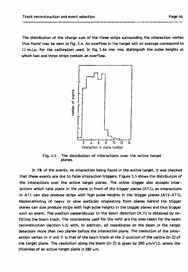
Fig. 5.5 The distribution of interactions over the active targetplanes.
In 3% of the events, no interaction being found in the active target, it was checkedthat these events are due to false interaction triggers. Figure 5.5 shows the distribution ofthe interactions over the active target planes. The online trigger also accepts inter-actions which take place in the plane in front of the trigger planes (ATI), as interactionsin ATI can also produce strips with high pulse heights in the trigger planes (AT2-AT7).Backscattering of heavy or slow particles originating from planes behind the triggerplanes can also produce strips with high pulse heights in the trigger planes and thus triggersuch an event. The position perpendicular to the beam direction (X.Y) is obtained by re-fitting the beam track. The coordinates used for the refit are the ones taken for the beamreconstruction (section 5.2) with, in addition, all coordinates on the beam in the targetdetectors more than two planes before the interaction plane. The resolution of the inter-action vertex in X and Y is that of the beam track at the Z-position of the centre (in Z) ofthe target plane. The resolution along the beam (in Z) is given by 280 jinW12, where thethickness of an active target plane is 280 urn.
Track reconstruction and event selection Page 47
5.5 Preselection
5.5.1 Introduction
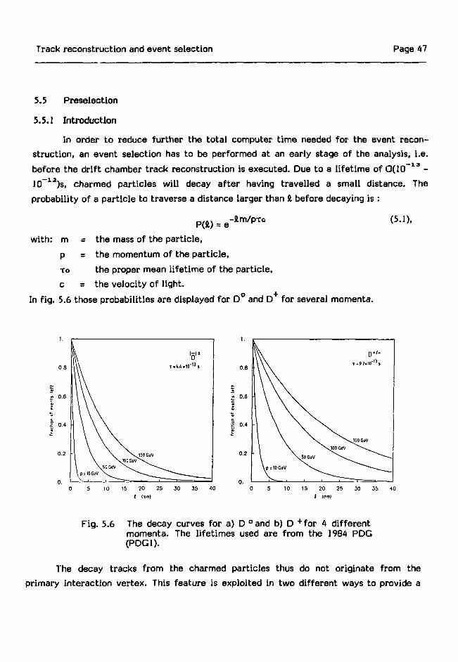
In order to reduce further the total computer time needed for the event recon-struction, an event selection has to be performed at an early stage of the analysis, i.e.before the drift chamber track reconstruction is executed. Due to a lifetime of 0(10~13 -10~12)s, charmed particles will decay after having travelled a small distance. Theprobability of a particle to traverse a distance larger than ft, before decaying is :
POl) = e - * m / p T 0
with: m = the mass of the particle,
p = the momentum of the particle,
TO the proper mean lifetime of the particle.
c = the velocity of light.
In fig. 5.6 those probabilities are displayed for D° and D for several momenta.
(5.1),
« 0.6
I 0.4
0 5 10 15 20 25 30 35 40 0 5 10 15 20 25 30 35 40
Fig. 5.6 The decay curves for a) D °and b) D +for 4 differentmomenta. The lifetimes used are from the 1984 PDG(PDG1).
The decay tracks from the charmed particles thus do not originate from theprimary interaction vertex. This feature is exploited in two different ways to provide a

Track reconstruction and event selection Page 48
preselection of the events. In the f i rs t preselection, events are selected which have tracks
which miss the primary vertex when extrapolated backwards f rom the vertex telescope,
the so-cal led impact parameter preselection. The second preselection looks for events
which exhibit a sudden jump in the charged part ic le mul t ip l ic i ty in the act ive target.
Events passing any of the two preselections are passed on for fur ther analysis. In the to ta l
preselection, 34% of the to ta l events sample are selected. In the fol lowing subsections, we
w i l l describe both preselections and assess their ef f ic iency for selecting charm decays.
5.5.2 Preselection on Impact parameter
As in the strong interact ion between the beam part ic le and the nucleons of the Si
nucleus the quantum number charm is conserved, only charm-ant icharm quark pairs can
be produced. When this pair does not form a bound state, the event w i l l contain two
charmed part ic les. We w i l l now make an estimation of the distance at which the decay
tracks w i l l miss the pr imary vertex when extrapolated backwards. In f i g . 5.7 some of the
quantit ies in this calculat ion are defined.
Plab2
Fig. 5.7 Def in i t ion of symbols for impact parameter calculat ion.I Interaction vertex, D decay vertex.
The distance b. . w i l l f rom now on be called the impact parameter. The sub- script
" lab" indicates that the value is taken in the laboratory system, " cm" indicates the rest
system of the decaying charmed part ic le. We can wr i te :
b lab = £ l a b s i n 0 l a b ™'with:
) (5.3).

Track reconstruction and event selection Page 49
and:
p = the momentum of the decay particle,cm
£ = the total energy of the decay particle,cm
0 = the angle with respect to the line of flight of the decaying particle,cm
(3 = the velocity of the decaying particle in the lab system relative to c,the speed of light
y = 1ATU-02).
The relation between the decay distance in the lab system and the proper lifetime t of the
decaying particle is :4 l a b = 0YCt (5.4).
For p l g b > 20 GeV : 3 « 1, thus :blab - c t Pcm^cAm^cmV <5-5>'
With charmed momenta > 20 GeV the impact parameters of the decay tracks are
thus independent of the momentum of the decaying charmed particle. For the two body
decay D° -» K~IT+ the maximum impact parameters for a lifetime of t = TQ are for ir and K
120 um and 103 um respectively. The impact parameter is linear in the lifetime of the
particle t, so we may expect impact parameters of the order of 50-500 um for two body
decays. For three and more body decays not all decay particles will have a large impact
parameter.
In the event preselection events are accepted which have two or more track pro-
jections in the vertex telescope which do not point back to the primary interaction vertex.
The reconstruction of track projections in the vertex telescope is done in four
steps, starting with the easiest tracks and successively going on to the more difficult
cases. Each of the steps is executed for the two full projections of three detectors in the
vertex telescope. In the first three steps a guide line is constructed connecting two co-
ordinates or a coordinate and the vertex. After this the coordinates in the other planes
are only considered if they lie within a distance of 0.2 mm from this guide line and have
not previously been used for another track. The final criterion for accepting a track
projection is a straight line fit with a cut on the resulting x . This x is the square of the
distances of the coordinates to the fitted track weighted for the coordinate errors. After
accepting a track its coordinates are deleted to prevent multiple use of coordinates. The
four steps are as follows.

Track reconstruction and event selection Page 50
2.
Reconstruction of tracks which point back to the primary interaction vertex
and have a hit in each of the three detectors of the projection.
For accepting the track the x2 (named x\, number of degrees of freedom
NDF = 3-2) from the straight line fit of the three coordinates should be less
than 6, corresponding to a cut on 2.8 standard deviations (a). The pointing
back condition is investigated by performing a straight line fit through the
three coordinates and the interaction vertex. This fit yields a x 3 (named
x2^, NDF = 4-2). To accept a track as pointing, it is demanded that x2. -
x2, < 6, which corresponds to a cut on 2.4 a.
Reconstruction of tracks which point back to the primary interaction vertex
and have a hit in the first two detectors of the projection, but miss the third
detector of the projection.
Such a track is accepted when a straight line fit of the two coordinates and
the vertex yields a x 2 less than 8.
QJ
• <D
B
C
-0.75 -0.50 -0.25 0.0b (mm)
0.25 0.50 0.75
F ig . 5.8 The impact parameter d is t r ibut ion fo r the t racksclassi f ied as non-point ing.
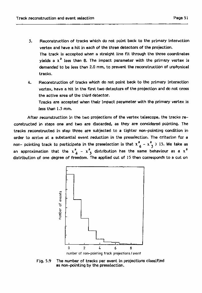
Track reconstruction and event selection Page 51
3. Reconstruction of tracks which do not point back to the primary interaction
vertex and have a hit in each of the three detectors of the projection.
The track is accepted when a straight line f i t through the three coordinatesyields a x 2 less than 8. The impact parameter with the primary vertex isdemanded to be less than 2.0 mm, to prevent the reconstruction of unphysicaltracks.
4. Reconstruction of tracks which do not point back to the primary interaction
vertex, have a hit in the first two detectors of the projection and do not cross
the active area of the third detector.
Tracks are accepted when their impact parameter with the primary vertex is
less than 1.5 mm.
After reconstruction in the two projections of the vertex telescope, the tracks re-
constructed in steps one and two are discarded, as they are considered pointing. The
tracks reconstructed in step three are subjected to a tighter non-pointing condition in
order to arrive at a substantial event reduction in the preselection. The criterion for a
non- pointing track to participate in the preselection is that x2^ - x2, > 15. We take as
an approximation that the x2. - x2^ distribution has the same behaviour as a x2
distribution of one degree of freedom. The applied cut of 15 then corresponds to a cut on
o
3
Fig. 5.9
number of non-pointing track projections/event
The number of tracks per event in projections classifiedas non-pointing by the preselection.

Track reconstruction and event selection Page 52
tracks having an impact parameter with the primary vertex larger than 4 c. Tracksreconstructed in step four are always taken for the preselection. In fig. 5.6 the impactparameters for the selected tracks are plotted. From fig. 5.8 it can be clearly seen thatthe 4 o cut on x \ - x3, introduces an effective impact parameter cut of 30 um.Figure 5.9 shows the number of tracks classified as non-pointing per event. The eventsample is reduced to 31% in this preselection step by demanding at least two tracks inprojection to be non-pointing.
5.5.3 Preselection on a jump in the charged multiplicity
This preselection uses the information supplied by the active target and multi-plicity counters. It selects events which exhibit an effective jump in the charged particlemultiplicity of 2 m.i.p. in the active target. For this the signal clusters in the multiplicitycounters and the interaction vertex are used to predict charge patterns in the activetarget. These charge patterns, series of signals in neighbouring planes caused by the sameparticles, are examined for multiplicity steps. A total multiplicity increase of 2 m.i.p. isrequired for selecting an event. This preselection accepts 3% of the events.
5.5.4 The efficiency of the preselection
The first preselection can exhibit an inefficiency with respect to the final analysis(section 5.8), where the tracks are reconstructed in space, using 2 full projections with 3VMSD counters each plus a counter with horizontal strips. Furthermore, the final recon-struction is guided by the drift chamber tracks. These extra facilities prevent the recon-struction of unphysical (ghost) tracks or distorted tracks and thus leave the coordinatesfor use with other correct tracks. The second preselection on charged multiplicity 'unripsin the active target will overcome most of the efficiency problems at low decay distancewhere the effect is expected to be worst. In order to check the efficiency of the pre-selection for tagging charmed particle decays which pass the impact parameter require-ments a comparison was done of the number of K° decays found in events accepted by thepreselection and events rejected by the preselection. The K° tracks were reconstructedwith a program analogous to the final charm analysis program discussed in sections 5.8and 5.9. The K°'s were required to have two track projections which miss the primaryvertex by 4 a. The results are summarized in table 11.
Track reconstruction and event selection Page 53
Table 11: Measured inefficiency of finding a K° decay
due to the preselection as function of the decay distance
Az (mm) inefficiency (%)0 - 5 0. ± 2.
5 - 1 0 5. ±2.
10-15 8. ±2.
15-20 9. ±2.
20 - 25 8. ± 2.
> 25 7. ± 2.
These inefficiencies are in fact an upper limit to the true inefficiencies as the
preselection tags events with non-pointing tracks, which do not necessarily come from the
particular decays to be selected. The decrease in inefficiency at decay distances of
0-5 mm is due to the second preselection on charge jumps in the active target. We con-
clude that the preselection gives no appreciable loss or bias on the charm decays recon-
structed with the final selection program.
In table 12 all event rejection factors are listed which occurred up to now in the
analysis. The average computer time spent per event up to this point is ~ 0.6 s/event (IBM
370/168 equivalent time).
Table 12: Event rejection in the first 3 analysis steps
decoding
beam track reconstruction
interaction vertex search
preselection
rejection rate (%)2.5
8.8
3.0
66.0
cumulative rejection rate2.5
11.1
15.8
71.7
5.6 Track Reconstruction in the Drift Chambers
The track reconstruction in the drift chambers of the spectrometer is done in a
program called ELFPRO. The program ELFPRO has been extensively described previously
in refs. PETE1, SPIE1 and DIJK1. The reconstruction proceeds in three steps.

Track reconstruction and event selection Page 54
1. First, track segments are reconstructed in the parts of the spectrometer where
no magnetic fields are present, and thus are straight lines. The field free parts
where the drift chambers are located are called ARMs (see fig. 2.2a). A track
traversing the complete spectrometer, i.e. which originates from the targetarea and leaves the spectrometer through the last (ARM3c) drift chamber,possesses one segment in the ARM2 drift chambers and one in the ARM3 driftchambers (see fig. 5.10). The track search is started in ARM3. As the trackmultiplicity in ARM3 is lower than in ARM2, the ARM3 search will be fasterdue to the smaller number of coordinates to be considered. The track segmentsreconstructed in ARM3 are subsequently used as guidance for the search inARM2 to restrict the search volume and thus to save time. After the guidedARM2 search a free ARM2 search is done with the still unused coordinates inARM2. The track segments in ARM2 and ARM3 are separately fitted with
straight lines.
2. When all track segments have been found and fitted a search for matches is
made between the ARM2 and ARM3 track segments. For all ARM2 and ARM3
segments the crossing point with the central plane of the BBC magnet is
calculated using a straight line extrapolation. The matching segments from
ARM2 and ARM3 cross, within errors, at common points. For segments in
ARM2 which do not enter the gap of the BBC magnet and segments in ARM2
and ARM3 to which no matching partner can be found it is checked whether
they point back to the primary interaction vertex in the Y-Z plane in which no
magnetic deflection takes place. This last match takes into account the
class vertex ARM1
IVMSD)
ARM2
(DC)
ARM3
(DC)
X
XMNP BBC
Fig. 5.10 The possible configurations of track segments in thespectrometer.

Track reconstruction and event selection Page 55
possible offset of tracks by several centimeters from the primary vertex due
to decaying particles originating from a decay at a displaced secondary
vertex. The reason for the absence of matching track segments is the high
beam intensity, due to which a narrow cylindrical region in the drift
chambers (radius ~ 1 cm) around the traversing non-interacting beam is
made in- sensitive by the accumulated space charge. Tracks crossing this
insensitive region can escape reconstruction in an ARM.
3. The last step in the drift chamber track reconstruction is a fit of thematched track segments or the single matched segments to the primaryinteraction vertex.Leftover track segments are not used any further in this analysis.
The result of the fit is a unit direction vector p of the track in the target area, an
associated momentum p and the charge polarity q of the particle. A track is then defined
by 7 parameters: X, X' = dX/dZ, Y, Y' = dY/dZ, Z, p and q. The errors on the track posi-
tion, direction and momentum and the correlation between the errors are represented by
the covariance matrix. This matrix has 15 independent elements :
var(X.X) covar(X.X') covar(X.Y) covarfX.Y') covar(X.p) \
var(X\X') covar(X'.Y) covatfX'.Y1) covar(X\p) *
var(Y,Y) covar(Y,Y*) covar(Y.p)
var(Y\Y') covar(Y'.p)
var(p,p)
The resulting tracks and momenta are used as guidance for the track reconstruction in the
vertex telescope. After finding the track segments in the vertex telescope a global refit
will be performed reusing the track segments yielding a more precise momentum
measurement (section 5.8). The configurations of segments which can form tracks are
depicted in fig. 5.10. The momentum resolutions for the tracks of different configuration
are given in table 6 of chapter 2.
5.7 Particle Identification
The Cerenkov counter hodoscopes are used to identify the particle on a track andthus to attribute a mass to the particle tracks (see ref. SPIE1). For the identification ofthe particles with the Cerenkov counter hodoscopes one calculates the expected numberof photoelectrons for each track in each Cerenkov hodoscope for the particle hypotheses:

Track reconstruction and event selection Page 56
proton, kaon and pion. The errors on these quantities can be calculated from the statis-tical significance of the photoelectron signal and the experimental detection errors. Usingthe measured number of photoelectrons in a counter, the probability can be calculatedthat the track is a proton, a kaon or a pion. The results for all counters which aretraversed by a track are multiplied :
Pj= IlPij (5.7)i
with: j = P.K.TT: the particle hypothesis,i = the Cerenkov counter hodoscope traversed by the track.
The light produced by several particles which overlaps in one mirror and lightoriginating from one particle covering several mirrors are taken account of in thisanalysis. The interpretation of the probabilities for the invariant mass calculation is basedon a comparison of the final probabilities for the three particle types. For some tracks theambiguities in the particle identification cannot be solved and they get a double particleassignment. In table 13 the particle assigments are listed as function of the measuredprobabilities.
The result of the particle identification is that the unit direction vector p and themomentum p as obtained from the drift chamber tracks can be extended into a fourvector (E,p$ for each particle hypothesis. The four vector (E,p) will be used later on in thecalculation of invariant masses for combinations of tracks.
5.8 Track Reconstruction in the Vertex Telescope
5.8.1 Global strategy
The four vectors obtained from the reconstruction in the downstream spectrometerdo not have a sufficient spatial resolution to allow for the reconstruction of decayvertices in the first few centimeters behind the target. To improve on this, theinformation from the vertex telescope is used. With the coordinates as found in thetelescope (see section 5.2) and guided by the drift chamber tracks we do a track segmentsearch, followed by a refit of the four vector resulting in a more precise measurement.
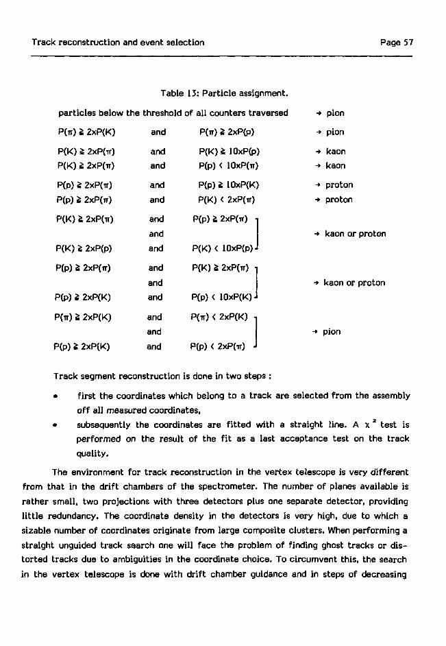
Track reconstruction and event selection Page 57
Table 13: Particle assignment.
particles below the
P(ir) £ 2xP(K)
P(K) i 2XP(IT)
P(K) £ 2XP(IT)
P(p) 2 2xP(ir)
P(p) 2 2xP(ir)
P(K) 2 2xP(n)
P(K) £ 2xP(p)
P(p) 2 2xP(ir)
P(p) 2 2xP(K)
P(ir) 2 2xP(K)
P(p) 2 2xP(K)
threshold
and
andand
andand
and
and
and
and
andand
and
and
and
of all counters traversed
P(ir) 2 2xP(p)
P(K) 2 10xP(p)
P(p) < 10xP(m)
P(p) 2 10xP(K)
P(K) < 2XP(IT)
P(p)2 2xP(ir) •
P(K) < 10xP(p).
P(K)2 2xP(ff) •
P(p)< 10xP(K).
P(IT) < 2xP(K) -.
P(p) < 2XP(TT) -I
-» pion
-» pion
-> kaon
-» kaon
-» proton
-» proton
-» kaon or proton
-» kaon or proton
-» pion
Track segment reconstruction is done in two steps :
• f irst the coordinates which belong to a track are selected from the assembly
off all measured coordinates,
• subsequently the coordinates are f i t ted with a straight line. A x 2 test is
performed on the result of the f i t as a last acceptance test on the track
quality.
The environment for track reconstruction in the vertex telescope is very different
from that in the drift chambers of the spectrometer. The number of planes available is
rather small, two projections with three detectors plus one separate detector, providing
l i t t le redundancy. The coordinate density in the detectors is very high, due to which a
sizable number of coordinates originate from large composite clusters. When performing a
straight unguided track search one wil l face the problem of finding ghost tracks or dis-
torted tracks due to ambiguities in the coordinate choice. To circumvent this, the search
in the vertex telescope is done with drift chamber guidance and in steps of decreasing

Track reconstruction and event selection Page 58
track quality. The track slope resolution (in the Y-Z plane) from the drift chambers is,due to the long lever arm in the spectromete., of the same order of magnitude as in thevertex telescope. Using this slope as a guide one overcomes to a large extent many of theproblems mentioned above. To recover low quality tracks which were not found in thesearch which was guided by the drift chambers, a second track search is done using thecombined guidance of the drift chamber tracks and the interaction vertex. The tracksearch strategy in the vertex telescope is schematically illustrated in fig. 5.11.
I initializationloop over quality
criteria for tracks-> -
drift chamber guided
micro track search- > -
end loop over
quality criteria
Tloop over guide points]
track search in projection 1 [
- | track search in projection 2 |
combine track projections
and hit in VMSO 5
fit of track candidate,
check x^ and signals
>-
1—
vertex/drift chamber guided
micro track search
t-I loop over guide points
select coordinates in
road around guide line
fit of track candidate,
check x and signals
global fit of micro strip/drift chamber tracks
—| end loop over guide points
select best track candidate
global f i t of micro stridrift chamber tracks
— | end loop over guide points )
Fig. 5.11 Scheme of the track finding strategy in the vertextelescope.
5.8.2 Track search guided by the drift chamber tracks
The drift chamber guided search is performed as follows.
• First we reconstruct a guide point in the centre of the MNP magnet for eachdrift chamber track (see fig. 5.12). This guide point represents the crossingpoint of the tracks in ARM1 and 2 in the absence of a magnetic field.
• A loop is started over these constructed guide points.

Track reconstruction and event selection Page 59
Subsequently a loop is done over the coordinates in planes three and four, the
so-called master planes, at +14° and -14° with the horizontal, respectively
(see f ig. 2.2). In the two main views of the telescope coordinates are selected
which lie in a road around the line connecting the coordinate in the master
plane and that on the guide point. In a similar way a coordinate in the
horizontal plane is also selected.
It is checked that this track candidate crosses the surface of a cylinder. This
cylinder is constructed around the beam axis, with a radius of 3 mm, starting
5 mm before th2 interaction vertex and ending at the first plane of the first
VMSD. All decays should take place in this volume. By imposing this condition
one prevents the reconstruction of unphysical ghost tracks.
1 2VMSD3 i. S 6 7
decayvolume
_ — ~~ " particle trajectory
14° V>° 0° U °
guide plane
X coordinate in VMSD
(g) guide point from DCs
+ interaction point
MNP magnet
Fig. 5.12 Schematic representation of the drift chamber guidance.
A track f i t is now performed through the coordinates in the vertex telescope
and the guide point giving a x 2 . This xa is required to be less than 70. This
limit was obtained in an empirical way in order to lose no tracks due to
cluster decoding distortions.
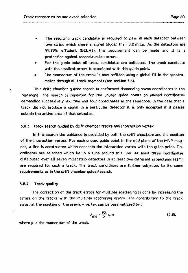
Track reconstruction and event selection Page 60
• The resulting track candidate is required to pass in each detector betweentwo strips which share a signal bigger than 0.2 m.i.p. As the detectors are99.99% efficient (BELA1), this requirement can be made and it is aprotection against reconstruction errors.
• For the guide point all track candidates are collected. The track candidatewith the smallest errors is associated with this guide point.
• The momentum of the track is now refitted using a global fit in the spectro-meter through all track segments (see section 5.6).
This drift chamber guided search is performed demanding seven coordinates in thetelescope. The search is repeated for the unused guide points on unused coordinatesdemanding successively six, five and four coordinates in the telescope. In the case that atrack did not produce a signal in a particular detector it is only accepted if it passesoutside the active area of that detector.
5.8.3 Track search guided by drift chamber tracks and interaction vertex
In this search the guidance is provided by both the drift chambers and the positionof the interaction vertex. For each unused guide point in the mid plane of the MNP mag-net, a line is constructed which connects the interaction vertex with the guide point. Co-ordinates are selected which lie in a tube around this line. At least three coordinatesdistributed over all seven microstrip detectors in at least two different projections (±14°)are required for such a track. The track candidates are further subjected to the samerequirements as in the drift chamber guided search.
5.8.4 Track quality
The correction of the track errors for multiple scattering is done by increasing theerrors on the tracks with the multiple scattering errors. The contribution to the trackerror, at the position of the primary vertex can be parametrized by :
ams = ^ u m (5>8)>
where p is the momentum of the track.
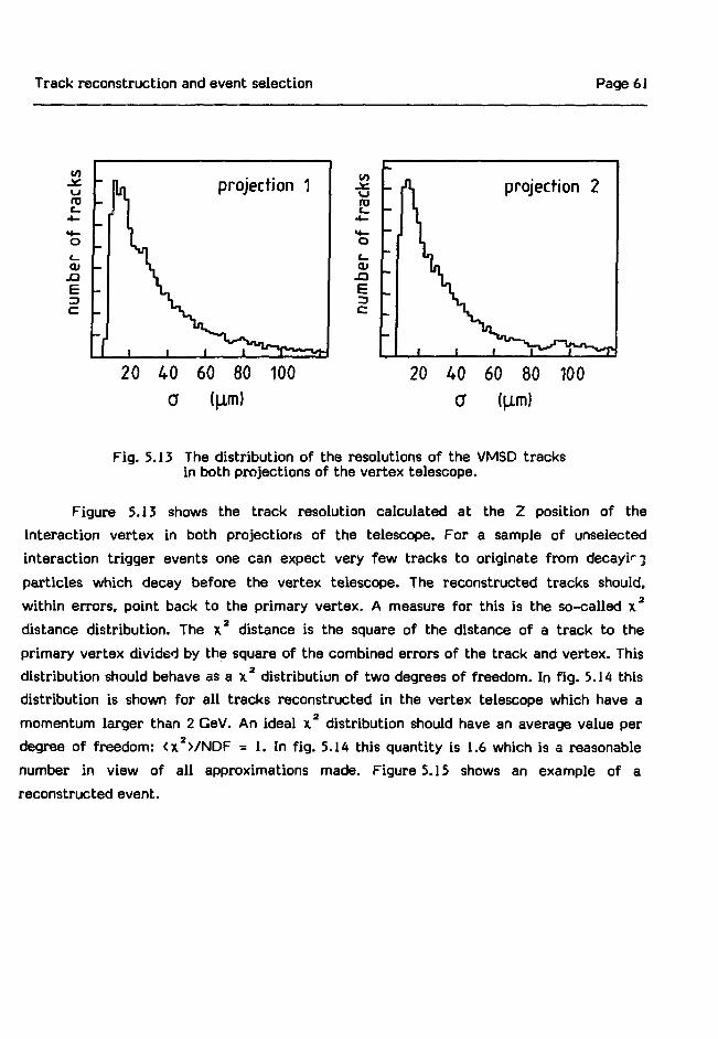
Track reconstruction and event selection Page 61
20 40 60 80 100
0
20 40 60 80 100a (|im)
Fig. 5.13 The distribution of the resolutions of the VMSD tracksin both projections of the vertex telescope.
Figure 5.13 shows the track resolution calculated at the Z position of the
interaction vertex in both projections of the telescope. For a sample of unselected
interaction trigger events one can expect very few tracks to originate from decayir'j
particles which decay before the vertex telescope. The reconstructed tracks should,
within errors, point back to the primary vertex. A measure for this is the so-called x2
distance distribution. The x2 distance is the square of the distance of a track to the
primary vertex divided by the square of the combined errors of the track and vertex. This
distribution should behave as a x2 distribution of two degrees of freedom. In fig. 5.14 this
distribution is shown for all tracks reconstructed in the vertex telescope which have a
momentum larger than 2 GeV. An ideal x2 distribution should have an average value per
degree of freedom: <x2>/NDF = 1. In fig. 5.14 this quantity is 1.6 which is a reasonable
number in view of all approximations made. Figure 5.15 shows an example of a
reconstructed event.
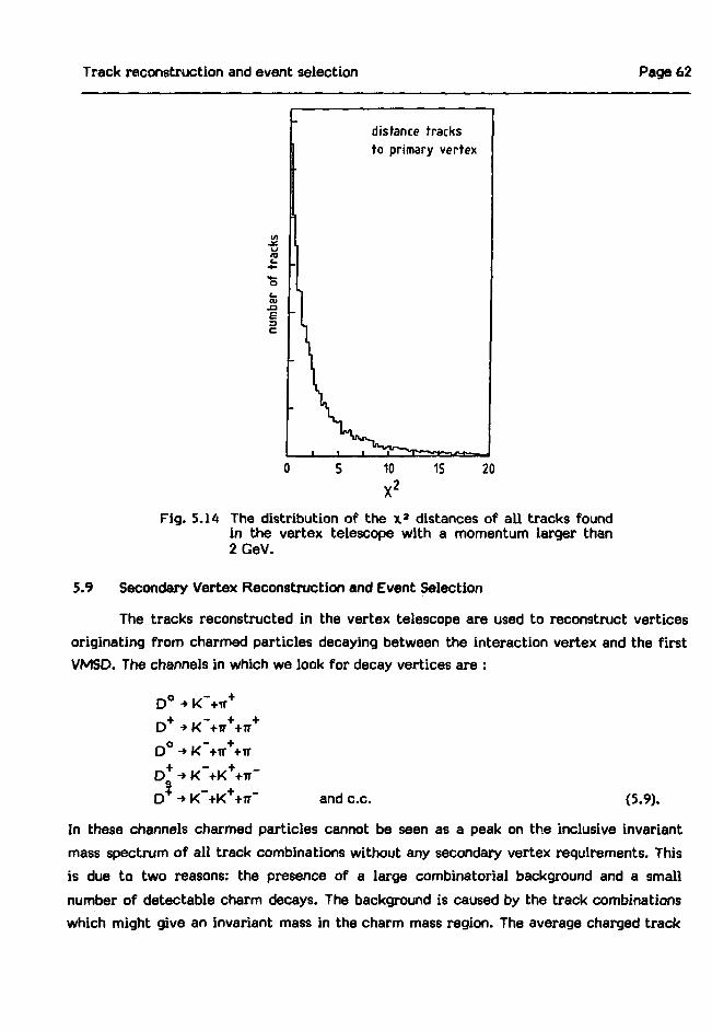
Track reconstruction and event selection Page 62
Ec
distance tracksto primary vertex
10 15 20
Fig. 5.14 The distribution of the x 2 distances of all tracks foundin the vertex telescope with a momentum larger than2GeV.
5.9 Secondary Vertex Reconstruction and Event Selection
The tracks reconstructed in the vertex telescope are used to reconstruct vertices
originating from charmed particles decaying between the interaction vertex and the first
VMSD. The channels in which we look for decay vertices are :
D°D » K + K + i rsD -• K~+K++ir~ and c.c. (5.9).
In these channels charmed particles cannot be seen as a peak on the inclusive invariant
mass spectrum of all track combinations without any secondary vertex requirements. This
is due to two reasons: the presence of a large combinatorial background and a small
number of detectable charm decays. The background is caused by the track combinations
which might give an invariant mass in the charm mass region. The average charged track
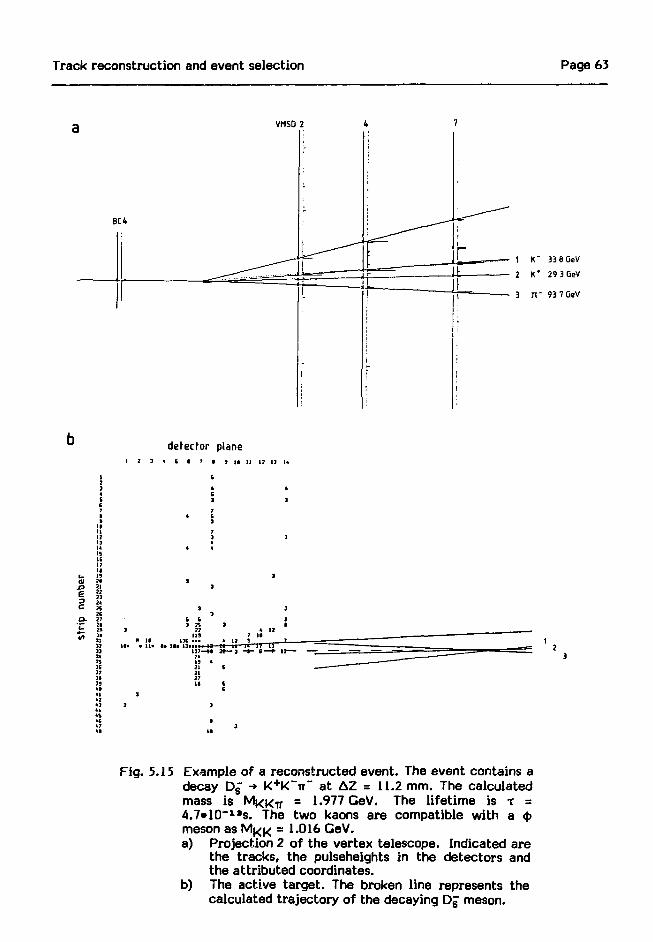
Track reconstruction and event selection Page 63
VMSD 2
BC4
1 K" 33 8 GeV
- 2 K* 2«3GeV
3 n" 93 7 GeV
01S3
detector plane
I I * • 1 1 . • • l l a 13aa<
Fig. 5.15 Example of a reconstructed event. The event contains adecay Dg •* K+K~ir~ at AZ = 11.2 mm. The calculatedmass is M K K ^ = 1.977 GeV. The lifetime is x =4.7*10~ias. The two kaons are compatible with a $meson as M « K = 1.016 GeV.a) Projection 2 of the vertex telescope. Indicated are
the tracks, the pulseheights in the detectors andthe attributed coordinates.
b) The active target. The broken line represents thecalculated trajectory of the decaying Dg meson.
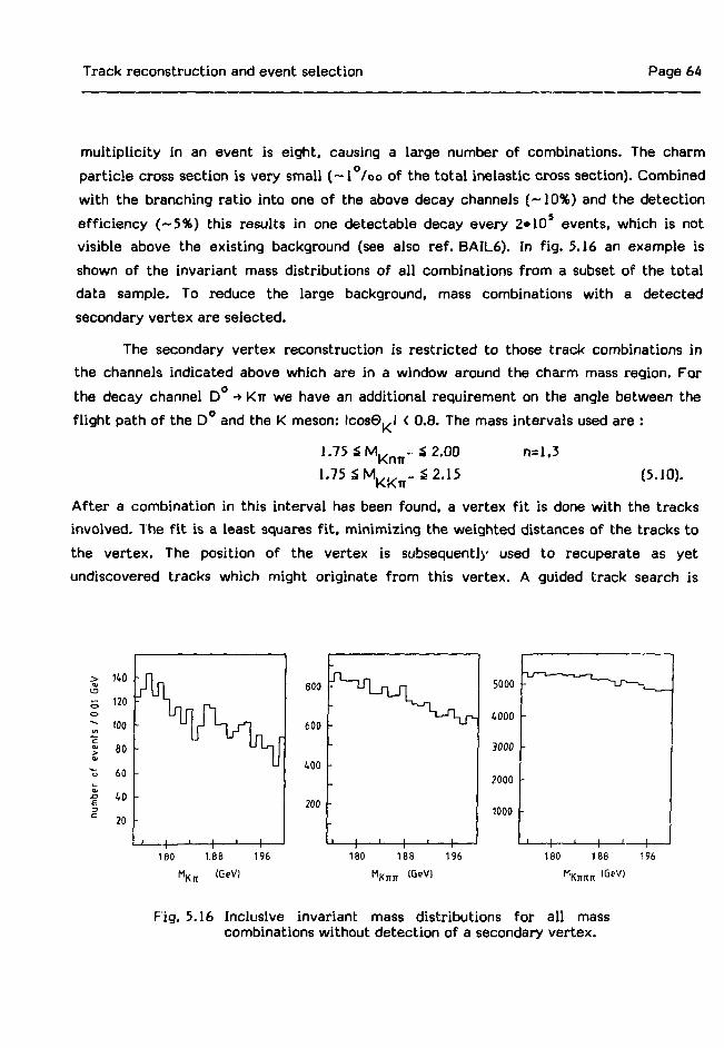
Track reconstruction and event selection Page 64
multiplicity in an event is eight, causing a large number of combinations. The charmparticle cross section is very small (~1 /oo of the total inelastic cross section). Combinedwith the branching ratio into one of the above decay channels (~10%) and the detectionefficiency (~5%) this results in one detectable decay every 2»105 events, which is notvisible above the existing background (see also ref. BAIL6). In fig. 5.16 an example isshown of the invariant mass distributions of all combinations from a subset of the totaldata sample. To reduce the large background, mass combinations with a detectedsecondary vertex are selected.
The secondary vertex reconstruction is restricted to those track combinations inthe channels indicated above which are in a window around the charm mass region. Forthe decay channel D -> Kir we have an additional requirement on the angle between theflight path of the D° and the K meson: lcos0,J < 0.8. The mass intervals used are :
1.75 £ M K r m - S 2.00 n=l,31.75 £ M,^_ - S 2.15 (5.10).
After a combination in this interval has been found, a vertex f it is done with the tracksinvolved. The f i t is a least squares f i t , minimizing the weighted distances of the tracks tothe vertex. The position of the vertex is subsequently used to recuperate as yetundiscovered tracks which might originate from this vertex. A guided track search is
140
120
too
80
60
40
20
Siu_J—1—1—1—1—1—
180 1.8B 196
(GeV)
Fig. 5.16 Inclusive invariant mass distributions for all masscombinations without detection of a secondary vertex.

Track reconstruction and event selection Page 65
made in projection (+14° and -14°) only, using the vertex position and the unusedcoordinates in the vertex telescope. If a track is found in one or both projections thesecondary vertex is considered to be incomplete, faking a decay vertex of one of thechannels (5.9), and rejected.
5.9.1 The selection criteria for secondary vertices
5.9.1.1 Selection criteria on the tracks
The reconstructed secondary vertices are subjected to a set of selection criteria.These selections are meant to reject all mass combinations not originating from a charmdecay vertex in that particular channel. In fact when all tracks are fitted with coordinateswhich exhibit pure Gaussian errors, and when those tracks are used for a vertex f i t , twocuts should be enough to reject the combinations not originating from a secondary vertex.These cuts are: a cut on the x2 of the fitted secondary vertex and a cut on the relativedistance, in terms of standard deviations, of the secondary vertex to the primary vertex.The former cut tests whether the tracks form a vertex, while the latter cut tests whetherthis vertex coincides with the primary vertex. In reality, however, the errors on the co-ordinates are not Gaussian, although they are represented and treated as such. Due tomultiple scattering, elastic scattering of the tracks in the microstrip detectors andcluster encoding distortions, the error distributions of the coordinates have a Gaussianshape extended with a tail. These tails are not very large with respect to the Gaussianpart, but they can introduce sizable effects in the vertex position and errors. To overcomethese problems more cuts are introduced which would, in the case of pure Gaussian errors,be equivalent with the two basic cuts. Now however these cuts will filter out distortedtracks and clean up our sample. These cuts are: cuts on the resolutions of decay tracks,cuts on the x2 distance of the decay tracks to the primary vertex and a cut on thedistance of secondary vertex to the primary vertex. A second class of cuts is still needed.Not all secondary vertices originate from charm decays in the channels mentioned in (5.9).These channels only represent ~15% of all decays. We will find additional secondaryvertices originating from:
• charm decays from which a low momentum track misses the acceptance ofthe drift chambers,
• charm decays with unobserved neutral decay products,
• secondary interactions,• vertices with wrongly assigned tracks.
Track reconstruction and event selection Page 66
To reject these combinations, cuts are applied to test whether the momentum sumvector of the decay points back to the primary vertex. In the case of secondary inter-actions other tracks may be attributed to the secondary vertex. A summary of the appliedcuts is given below.
• A cut on the x a of the secondary vertex. The x 2 cut is set to correspond to aconfidence level of 1%, 1% and 10% for respectively 2, 3 and 4 prong decays.
• A cut on the weighted distance of the secondary vertex to the primary vertex.The distance is required to be bigger than 4 a.
• A cut on the distance of the secondary vertex to the primary vertex. Thedistance should be larger than 3 mm.
• Cuts on the xHi8tance o f t h e d e c a v t r a c k s t o t n e primary vertex.
For 2 prong decay: one track with ^'stance > * ' " i e o t ' i e r w* t n x d ' t * 4"For 3 prong decay: two tracks with *Histance > 9< fc^6 o t n e r w ' ^ x distance > 4 'For the KKir decay channels, the last requirement was decreased to x i t >1, as the additional selected kaon provides the necessary background reduction.For 4 prong decay: two tracks with Xj. t a n c e > 9, one other with x!- t > 4.
• A cut on the resolution of the decay tracks. The decay is required to have atleast two track projections (in the vertex telescope) with a resolution better than
A cut to test whether the momentum sum vector of the decay points back to the
primary vertex. The xHietance °^ t l i e t r a J e c t o r v °f t n e reconstructed charmdecay candidate with respect to the primary vertex should be less than 12.Cuts on the attribution of leftover tracks to the various vertices. Two types ofleftover tracks can be present, tracks found with drift chamber guidance andtracks only seen in the vertex telescope. A track can be attributed to a vertexwhen it has a weighted impact parameter of less than 3 a and in both projectionsa resolution better than 30 ym.Of the tracks which cannot be attributed to the primary vertex only one isallowed to point to the secondary vertex.
Track reconstruction and event selection Page 67
Only one extra track reconstructed in a vertex telescope projection without drift
chamber guidance is allowed to point to the secondary vertex while being
incompatible with the primary vertex.
Tracks which point back to neither of the two vertices are used in a search for a
third vertex.
Only one track is allowed to point back to none of the three vertices.
5.9.1.2 Selection criteria using tracks and active target
The aim of an active target consistency cut is to check whether tracks, which are
considered as decay tracks, can be recognized as coming from the primary vertex from
the pulse height in the active target. As a first step all tracks in the event which have axdistance °^ *ess t ' 1 a n ^ a r e c ' a s s ^ ' e c ' a s P°intin9 t o the primary vertex. These "pointing"
tracks are then displaced parallel to themselves towards the primary vertex. Subsequently
the n;ilse heights in all planes of the active target downstream of the interaction vertex
are calculated. For the calculated pulse heights it is assumed that a particle deposits a
charge equivalent to 1 m.i.p. in each plane divided over the two nearest strips. The
calculated pulse height for each strip is then summed for all "pointing" tracks. The
calculated and measured pulse heights in the pairs of strips covered by the decay tracks
which were classified as "pointing" are then compared with each other. The Landau
distribution has, as function of the pulse height, a steep rise to a maximum followed by a
slower descent into a long tail (see figs. 3.2 and 4.4). If a pulse height is measured which is
bigger than the one calculated, no statement can be made as to whether these are
compatible with each other, due to the tail from the Landau distribution. However, if the
measured pulse height is smaller than the one calculated, and lower than the pulse height
at the onset of the distribution, the measured pulse height can be considered to be
incompatible with the calculated. In that case one may conclude that fewer particles have
passed than presumed from the "pointing" classification. The compatibility is checked by
taking the difference between the measured and the calculated pulse heights. For the
planes in which the measured pulse height (ph) is smaller than the calculated, these
differences are added in quadrature and divided by the number of planes behind the
interaction plane (5.11). To consider a track not present, i.e. incompatible with the active
target, this value should exceed 0.2, which corresponds to a level of 0.45 m.i.p.; we use :

Track reconstruction and event selection Page 68
measured ~ p calculated'
planes
For 3 and 4 prong decays it is allowed that at most 1 track is compatible with the primaryvertex according to the target information. For 2 prongs this test is not made, as it doesnot change the signal over background ratio.
Using the reconstruction and selection as described in this chapter events areselected. These events, their mass spectra and the extracted lifetime results are pre-sented in the next chapter.

Mass spectra and lifetimes of charmed mesons Page 69
6. MASS SPECTRA AND LIFETIMES OF CHARMED MESONS
6.1 Introduction
In this chapter we will present the selected events as obtained with the selectioncriteria described in chapter 5. The chapter is organized as follows: first we will discussthe method to extract the lifetime from a sample taken with a restricted efficiency asfunction of the lifetime, then we will discuss the treatment of the background. In thefollowing sections we will present the selected data sample and the lifetimes obtained.Systematic biases will also be discussed.
6.2 Lifetime Determination Via Measurement of Decay Length
In this section we will give a description of the method employed to determine the
mean lifetime of a particle via the measurement of the decay length.
The probability of a particle to decay per unit time is taken to be X. In total we
have N particles from which dN decay in a time interval d t :
dN = -N\dt , and hence N = Noe"^ (6.1),
with: No the initial number of particles at t = 0.
We can now define T = l / \ which is the mean lifetime of the particle. The
probability to observe a particle which decays with a lifetime between t. and t.+dt. is then
e-' i / Tdt K
with: k. the probability to observe a decay independent of lifetime.
When the particle is only observable in a certain time interval [t ir,,t ], thenrnin msx
the normalization factor in the denominator of (6.2) becomes an integral between t .
a n d 'max :
k. e- f c i / T dt .p ( f c > - - T s s r — r s s i r (63)

Mass spectra and lifetimes of charmed mesons Page 70
In the case that t.max )> x, i.e. the length of the decay volume is long with respect to the
mean decay length, (6.3) becomes :
k. . min. .P(tj)= -7 e-^i-'i Vx dt. (6.4).
This is again an exponential decay distribution but now in the so-called "corrected" l ife-
time t . - t [n i n .
When a sample of N particles is detected, then their mean lifetime x can be extracted
using the likelihood function L :
LW M I 1
The lifetime is obtained by maximizing the logarithm of L with respect to t .
In reality the individual lifetimes of the particles are obtained from three quan-
the traversed distano
the mass of the particle m. :
tities: the traversed distance 1. from production to decay vertex, the momentum p. and
m.c 2 I.fci=^ * - c <6-6>-
In the following subsections we will elaborate on the method to extract the lifetime from
the observed events. In particular the effect of the background on the lifetime and the
detection efficiency as function of the decay distance will be discussed.
6.2.1 Detection efficiency
The detection efficiency for an event with certain kinematical properties can be
approximated with a block shaped efficiency function. Below a time t m i n the efficiency
is zero, between t m i n and t m a x the efficiency has a constant value, above t m a x the
efficiency is again zero. Interpreting the time interval [ t m i n , t m a x ] as a time interval in
which the decay is visible, the values of t m i n and t m a x can formally be regarded to have
no errors. The measurement errors will however vary for decays of each decay channel, as
the environment depends on additional tracks which influences the attribution of errors to
the coordinates in the vertex telescope. These differences occur due to e.g. Landau
fluctuations, elastic scattering in the silicon detectors and the influence of the charge
deposited due to the other tracks in the event. The efficiency function will thus
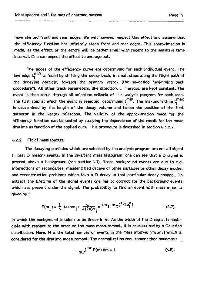
Mass spectra and lifetimes of charmed mesons Page 71
have slanted front and rear edges. We will however neglect this effect and assume that
the efficiency function has infinitely steep front and rear edges. This approximation is
made, as the effect of the errors will be rather small with regard to the sensitive time
interval. One can expect the effect to average out.
The edges of the efficiency curve are determined for each individual event. The
low edge t m i n is found by shifting the decay back, in small steps along the flight path of
the decaying particle, towards the primary vertex (the so-called "swimming back
procedure"). All other track parameters, like direction- ... * errors, are kept constant. The
event is then rerun through all selection criteria of '•"••* ..nalysis program for each step.
The first step at which the event is rejected, determines t m i n . The maximum time t.ma*
is determined by the length of the decay volume and hence the position of the first
detector in the vertex telescope. The validity of the approximation made for the
efficiency function can be tested by studying the dependence of the result for the mean
lifetime as function of the applied cuts. This procedure is described in section 6.3.2.2.
6.2.2 Fit of mass spectra
The decaying particles which are selected by the analysis program are not all signal
(= real D meson) events. In the invariant mass histogram one can see that a D signal is
present above a background (see section 6.3). These background events are due to e.g.
interactions of secondaries, misidentified decays of other particles or other decay modes,
and reconstruction problems which fake a D decay in that particular decay channel. To
extract the lifetime of the signal events one has to correct for the background events
which are present under the signal. The probability to find an event with mass m.±o. is
given by :
P(m.)= 1 (a+bm.+ 7 ^ . ^ ^ ^ / 2 < > (6.7),
in which the background is taken to be linear in m. As the width of the D signal is negli-
gible with respect to the error on the mass measurement, it is represented by a Gaussian
distribution. Here, N is the total number of events in the mass interval [mi.ms] which is
considered for the lifetime measurement. The normalization requirement then becomes :
m i rm a P(m) dm = 1 (6.8).
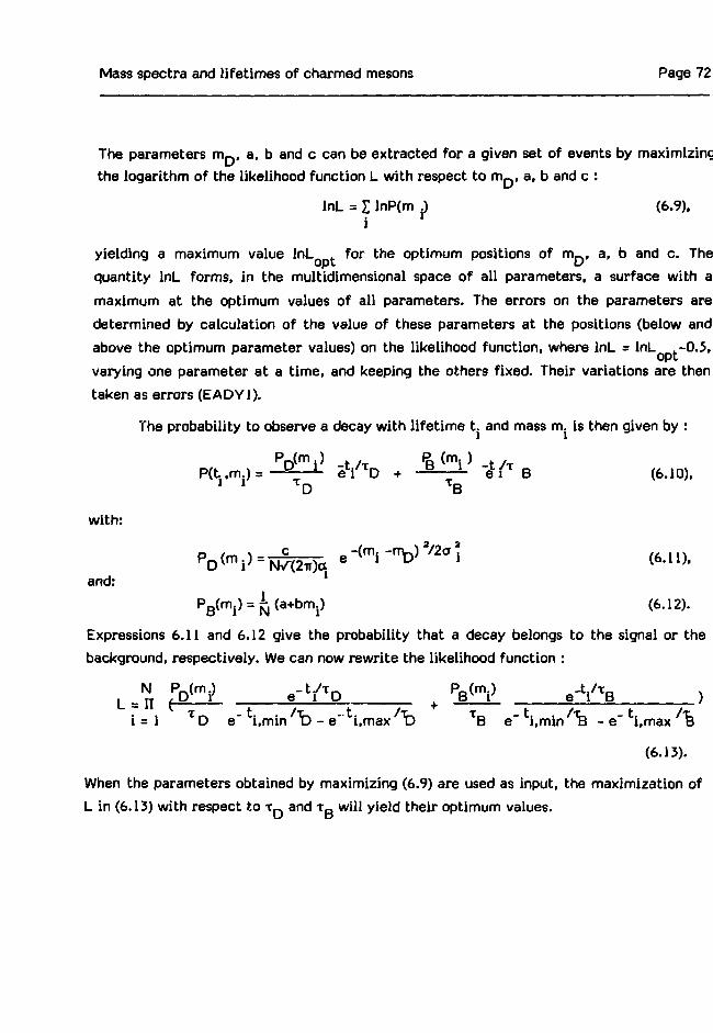
Mass spectra and lifetimes of charmed mesons Page 72
The parameters mD> a, b and c can be extracted for a given set of events by maximizingthe logarithm of the likelihood function L with respect to rrip, a, b and c :
lnL = £ lnP(m .) (6.9),i
yielding a maximum value lnL t for the optimum positions of m_, a, b and c. The
quantity lnL forms, in the multidimensional space of all parameters, a surface with a
maximum at the optimum values of all parameters. The errors on the parameters are
determined by calculation of the value of these parameters at the positions (below and
above the optimum parameter values) on the likelihood function, where lnL = lnL .-0.5,opt
varying one parameter at a time, and keeping the others fixed. Their variations are then
taken as errors (EADY1).The probability to observe a decay with lifetime t. and mass m. is then given by :
Pn(m.) t / Pa (m.) t /P(t,m.) = — - — L i Y T D + — - ~&V B (6.10),
1 1 XD TB
with:
and: 'PB(m.) = Jj (a+bmp (6.12).
Expressions 6.11 and 6.12 give the probability that a decay belongs to the signal or thebackground, respectively. We can now rewrite the likelihood function :
i = 1 T D e" i.min fa - e" i.max fa e i,max
(6.13).
When the parameters obtained by maximizing (6.9) are used as input, the maximization ofL in (6.13) with respect to T D and T B will yield their optimum values.

Mass spectra and lifetimes of charmed mesons Page 73
6.2.3 The influence of the measurement errors of the lifetime of individual events on
the mean lifetime
The lifetime of each individual decay is measured with a finite measurement
error. To check the effect of an error on the individual lifetime, we used a Monte Carlo
program in which a lifetime distribution was generated. Subsequently the distribution was
smeared, by shifting each individual value with an error value as drawn from a Gaussian
error distribution. A f i t to the smeared curve was performed to obtain again a lifetime.
For various assumptions on the error distributions, the difference with the original
generated lifetime was smaller than 2%. In the f i t we can thus omit the error on the
individual l ifetime, as our statistical error exceeds this value.
6.3 Results
6.3.1 Mass spectra from the selected events
The invariant mass distributions for the selected events are presented in figures 6.1
and 6.2. In f ig. 6.1 the mass distributions for the decay channels D° -»Kir,
D -» KTTTT and D° •* KtririT are given for the two different beam types K~ and IT" as well as
for the total data set. In all distributions the signals for the D mesons stand out clearly
above the background. In fig. 6.2 the mass distributions are shown for the decay channels
D -» KKTT and D -> \<Kn. The mass distribution for the K~ data shows an accumulation of
events around the D+ mass. From the 10 events seen in the D* mass region, 3 have aKK
mass compatible with a $ meson. Only one event is due to a D , the rest originate from
D~. The signal due to D -» KKir is either very small or absent. In the distribution for thesir~ beam no evidence is seen for either decay mode. This seems to indicate that D"
production is favoured with the K~ beam, in which case the strange valence quark of theD~ originates from the K~ (leading particle effect). However, no enhancement of D+
s
production with a K~ beam is expected, which is confirmed by the absence of a
D+ -» K+K~n+ signal as seen in the ir~ beam.
For all channels the number of signal and background events, as f i t ted with an
algorithm described in section 6.2.2, are presented in table 14.

Mass spectra and lifetimes of charmed mesons Page 74
n~beam K"beam sum
sum D -> Kn and D° -> Knnn
1.80 1.88 1.96 1.80 1.88 1.96 1.80 1.88 1.96Mass (GeV)
Fig. 6.1 The invariant mass distributions for the selected eventsin the channels D° -> Kir, D+ -» Kirir and D° -» Kirwir, forincoming ir~ and K~, and for their sum- The lines arethe results from the fits in the mass window 1.75 to2.00 GeV.

Mass spectra and l i fet imes of charmed mesons Page 75
OO
aj-O
C
8 -
1 6
£ 42 h
8
6
4
2
- fin•A,
-
"JJl
D+
fl , fl p
inJ ln jL_1L.
i
n
—
h
| r
n_
a
nlinr
b
i i i
c
1.80 i.9O 2.00 2.10
M KKK
Fig. 6.2 The invariant mass distributions for the selected eventsin the channels D j -»KKir and D+ -»KKir, the dottedevents are ambiguous with the decay D+ -»K-rnr,a) incoming IT" beam, b) incoming K~ beam and c) alldata. The line in b) is the result from the f i t in the masswindow 1.9 to 2.15 GeV, above the D+ mass.
Table 14: Number of f i t ted signal and background events
decay channel
D°-»KTT
D+ -• Kirir
D° -* K-rrinr
D ° -» Kir+D° -» KTTTTTT
D + •* K K T T *
mass (GeV)
1.863±0.002
1.871 ±0.002
1.864±0.001
l.S64±0.001
1.978±0.005
number ofsignal events
24±5
34±5
26±6
48±8
8
number ofbackground events
5
4
12
16
2
not fitted, see section 6.3.3.

Mass spectra and lifetimes of charmed mesons Page 76
6.3.2 The lifetimes of the D° and D+ mesons
6.3.2.1 Lifetime determination
For the events in the mass distributions displayed in fig. 6.1 we perform the
lifetime fit as described in the previous section. The lifetimes for the D meson from the
Kirir channel, for the D° meson from the Kir and KiririT channel as well as for the sum of
the last two are given in table 15. The lifetime of the background is also given. The
lifetime of the background is significantly smaller than the lifetime of the signal,
indicating that the background may be due to reconstruction accidents resulting in short
distance vertices and due to secondary interactions in the active target, which occupies
the first few mm of the decay volume. In fig. 6.3 the corrected lifetime distributions are
shown for the events in the signal regions. The curves represent the fitted lifetimes which
also contain a component for the background.
Table 15: Results of the lifetime fits for D° and D+.
background ( 1° s)
1.7±°-4
decay channel
DP * Kn
D+ -» Kirn
D° ->Ktrtrn
D° -» Kir or KirTrtr
Signal <10 s>
O . 9
1 . 6
O . «
3.8±°-7
O.3
0.9±°-3
O.2
1.8±O>2
0.2
1.8±°'2
6.3.2.2 Systematic errors
When measuring the lifetime of a particle via the measurement of the flight path
of individual events we take into account the detection efficiency as function of the
length of the flight path by defining the minimum and maximum detectable lifetimes (see
section 6.2.1). To check the validity of our procedure we vary several cuts which are
sensitive to the decay distance (Az, x .. t ) and determine the lifetime again. When
the assumption on the shape of the efficiency curve was correct and the swimming back
procedure was correctly executed we should arrive at the same lifetime, within errors, for
each set of cuts. Some caution is necessary in interpreting the results, as the events
samples are not statistically independent.
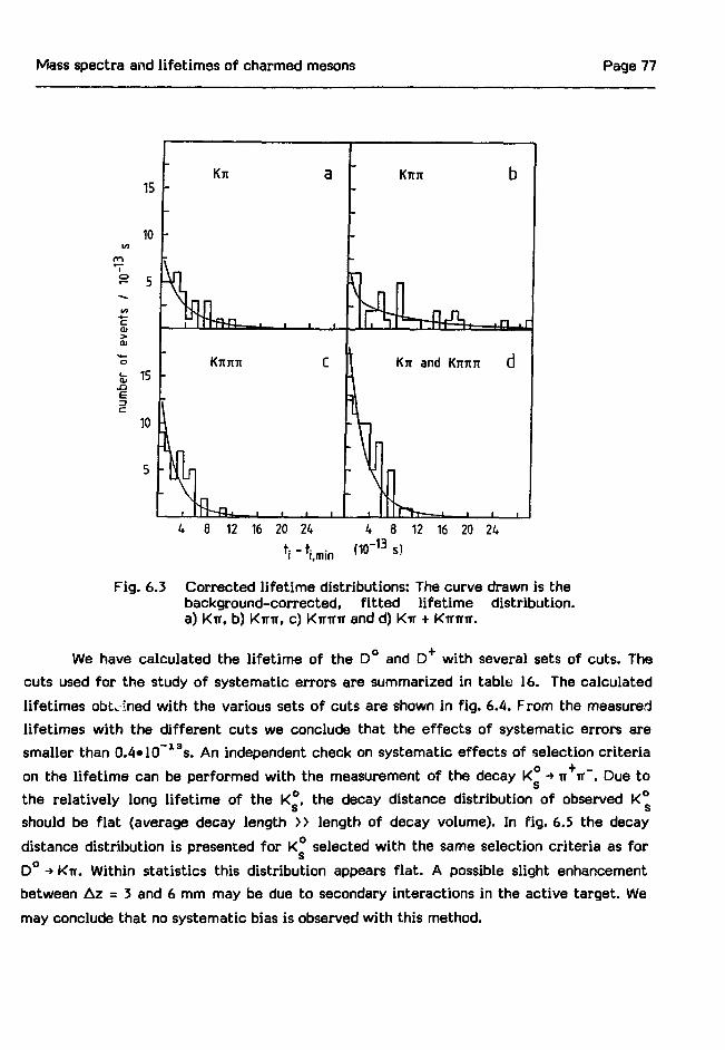
Mass spectra and lifetimes of charmed mesons Page 77
4 8 12 16 20 24
i.min
4 8 12 16 20 2410~13 s)
Fig. 6.3 Corrected lifetime distributions: The curve drawn is thebackground-corrected, f i t ted lifetime distribution,a) Kir. b) Kinr, c) Kiririr and d) Kir + KiTTrtr.
We have calculated the lifetime of the D° and D+ with several sets of cuts. The
cuts used for the study of systematic errors are summarized in table 16. The calculated
lifetimes obtained with the various sets of cuts are shown in fig. 6.4. From the measured
lifetimes with the different cuts we conclude that the effects of systematic errors are
smaller than 0.4*10~13s. An independent check on systematic effects of selection criteria
on the lifetime can be performed with the measurement of the decay K° -»ir -IT". Due to
the relatively long lifetime of the K°, the decay distance distribution of observed K°s s
should be fiat (average decay length >> length of decay volume). In fig. 6.5 the decay
distance distribution is presented for K° selected with the same selection criteria as for
D° -» KTT. Within statistics this distribution appears f lat. A possible slight enhancement
between Az = 3 and 6 mm may be due to secondary interactions in the active target. We
may conclude that no systematic bias is observed with this method.
Mass spectra and lifetimes of charmed mesons Page 7£
D+
A
=
U
5
Z
1c
605040
302010
;I I
1 • • i
—L— ,
1—iii
i i
I
i
I
--i
I
"" *
i
i
i_
- — — (
i
I
—1
- - ii i
b
I
—1
I;
-—=---4 —
7
54S3 h2 -1
m
0/
*o
1e3C
60SO40302010
~ ^ 1
— i
. 1
I i L T L J .
a .
-
-1 -
-
13 H
1211 I10 i9 -
set of cuts set of cuts
Fig. 6.4 The lifetimes as obtained with various sets of cuts. Thecuts are listed in table 16. Sets 1 to 4 are for the firstgroup in table 16, sets 5 to 9 for the second group. Set3 and set 6 are identical. In each picture the top plotsgives the lifetime results, the drawn histogram thesignal and the broken line histogram the backgroundbelow the signal, a) Kir, b) Kir + Kirnir.
E
e 15
c<u
5 10O
Qi
- Ifr H8 16 24
AZ (mm)32
Fig. 6.5 DistributionK£ -»ir+ir".
of the decay distance of

Mass spectra and lifetimes of charmed mesons Page 79
Table 16: The cuts used for the systematics study.
The cuts which are not varied remained as described in section 5.9
cutset Az(mm) a x a distance f ° r closest, 2nd closest and 3rd closesttrack to the primary vertex
1 3 4
5 2
6 3
7 4
8 5
9 6
Kir0
4
0
9
4
9
9
9
4
9
4
9
4
9
4
9
4
9
Kir IT0
4
9
0
9
9
4
9
9
9
9
9
4
9
9
4
9
9
4
9
9
4
9
9
4
9
9
KITITTr0
0
4
0
0
9
0
4
9
0
9
9
0
4
9
0
4
9
0
4
9
0
4
9
0
4
9

Mass spectra and lifetimes of charmed mesons Page 80
6.3.3 The lifetime of the D* meson
For the determination of the D+ lifetime we will use the data obtained with the
K~ beam, as only in this subsample a clear signal is visible above the background. To avoid
distortions due to decays which are ambiguous (in particle identification) with the decay
D+ -> Kinr, we do not include events, if they have a KTTTT mass in the range: 1.85 < fvi <KTT7T
1.90 GeV (see fig. 6.6a). As can be seen from fig. 6.2, the number of events available forthe determination of the D+ lifetime is very limited, due to which a fit of the lifetimewill gain us little precision. Therefore we will only make an average of the individuallifetimes corrected for background. To study possible systematic effects of thebackground on the lifetime, we try to clean up the KKir mass spectrum by scanning theevents, because in a small sample background events can have a large impact. We willdiscuss three cases, one without any scanning criterion, and two cases with successivelytighter scanning criteria.
1. For the event sample as shown in fig. 6.6a which is selected without scanning
criteria, the lifetime of signal and background are presented in table 17,
row 1. In fig. 6.7 the corrected lifetime distributions are shown for the events
in the signal regions, the curve representing the average lifetime which
contains a component for the background. The lifetime of the background is
taken as the average from the events in the mass windows 1.90 < M <
1.95 GeV. 2.00 < M < 2.15 GeV
2. The event sample is cleaned up by a visual scan of individual events. The scanis performed on an Apollo work station with a visual display terminal. Thepurpose of the scan is to recognize either wrongly reconstructed primaryvertices or secondary interactions in the target. Wrongly reconstructedprimary vertices are recognized from the target information together withthe tracks from the vertex telescope. They are mostly due to backscatteredheavy fragments in the active target. Secondary interactions are found againby visually combining track and target information. If the target contains alarge excess of charge in the neighbourhood of the secondary vertex andextra tracks seem to originate from the same region, one can classify theevent as a secondary interaction. In fig. 6.6b the resulting mass spectrum ispresented. The scan clearly rejects background events while the signalremains. In table 17, row 2, the lifetime results for this sample are given.

Mass spectra and lifetimes of charmed mesons Page 81
8
6
4
o-~ 8
;ven
H—
o 2
c
i s6
4
2
-
-
r ^ .fl-
mrH .n
nri.n
A
A
A
n.
n i
n •
a
b
. r
c
-Ml
Fig. 6.6
1.80 1.90
MKKn
2.00
(GeV)
2.10
The mass distributions for the K "beam data in the KKTTchannel, a) no scan, b) scan to reject secondaryinteract ions and wrong pr imary vert ices, c) scan as b)but to also reject wrong reconstruction.
1O
"cCD
01
4—
ocu
eC
15
10
5
KKn-
-
--
j n
4 8 12 16 20 24
•i-^min ( 1 0 " 1 3 s )
Fig. 6.7 Corrected lifetime distribution for KKir. 1 he curvedrawn is the background-corrected, average lifetimedistribution for KKn (case 1).

Mass spectra and lifetimes of charmed mesons Page 82
3. With the second set of scanning criteria we reject, in addition to the criteria
in case 2, also reconstruction errors which are clearly contradicted by the
active target information. Wrong reconstructions are vertices found with
tracks originating from different vertices, but which are combined into a
fictitious secondary vertex. Wrong reconstructions can be rejected if decay
tracks are seen in the active target, but are evidently not originating from
the reconstructed vertex. On the basis of this scan we arrive at the mass
distribution as depicted in fig. 6.6c. The results for the lifetime are given in
table 17, row 3.
From the study of the influence of the background on the lifetime, we conclude that no
appreciable effect can be seen. We have checked that the result without scanning, and
thus without bias, is stable within the errors.
Table 17: Lifetime results for the D* meson.
1) no scan, 2) scan to reject secondary interactions and wrong primary vertices, 3) scan as2, but also reject wrong reconstruction.
case mass(GeV) number of number of ts ]gna ] ^backgroundsignal events background (10 13s) (10 "s )
events
1 3.6±1-1 2.4±1.0
1 3.6±1-1 2.2±1.01.5
1 3.9±1#a 2.9±1.7a.7
6.4 Comments on the Relative Production Rates of Charmed Particles
From the total number of events measured with incoming K ~ beam and incomingn~ beam . we can extract the relative cross section for the production with the two beamtypes. These numbers can be stated under the assumption that the acceptance of thespectrometer is equal for both K~ and n" production. The cross section ratios obtainedare :
1
2
3
1.974±0.005
1.974±0.005
1.971 ±0.004
8
8
7

Mass spectra and lifetimes of charmed mesons Page 83
q(K-Si-»DoA ) _ 37±7 NQQ _
oiK~Si-»cP ) 23±5 x= 2 5 ± 6 N<K">
14±4 N(TT~)
We may conclude that the production rates in the K~ beam are of the same order of
magnitude as those in the TT~ beam within the Feynman x._ range (about 0 to 0.9) covered
by the spectrometer (see ref. NEUC1).
6.5 Conclusions
The results for the lifetimes of the D+, D° and D* mesons are :
T(D+) = 9.5±^±0.4«lCf13s
T(D°) = 3.8±^±0.4«10"19s
x(D*) = 3.6±i:i±0.4»10~13sS 1.5
The errors given are statistical and systematic, respectively. The results for the lifetimesof the three types of D mesons are all obtained with the same apparatus and practicallyequal selection. Hence, it can be expected that systematic biases cancel out in ratios ofthe lifetimes. The lifetime ratios obtained are :
T(D+ ) /T(D°) = 2.5±0.6
+ * ) = 2.6tl.ls
) / T ( D ) a 0.9±0.4
The errors for the ratios were obtained by averaging the asymmetric individual errors
followed by a standard error propagation.
The production rates in the K beam are of the same order of magnitude as those in theIT" beam within in the xp range covered.

Page 84
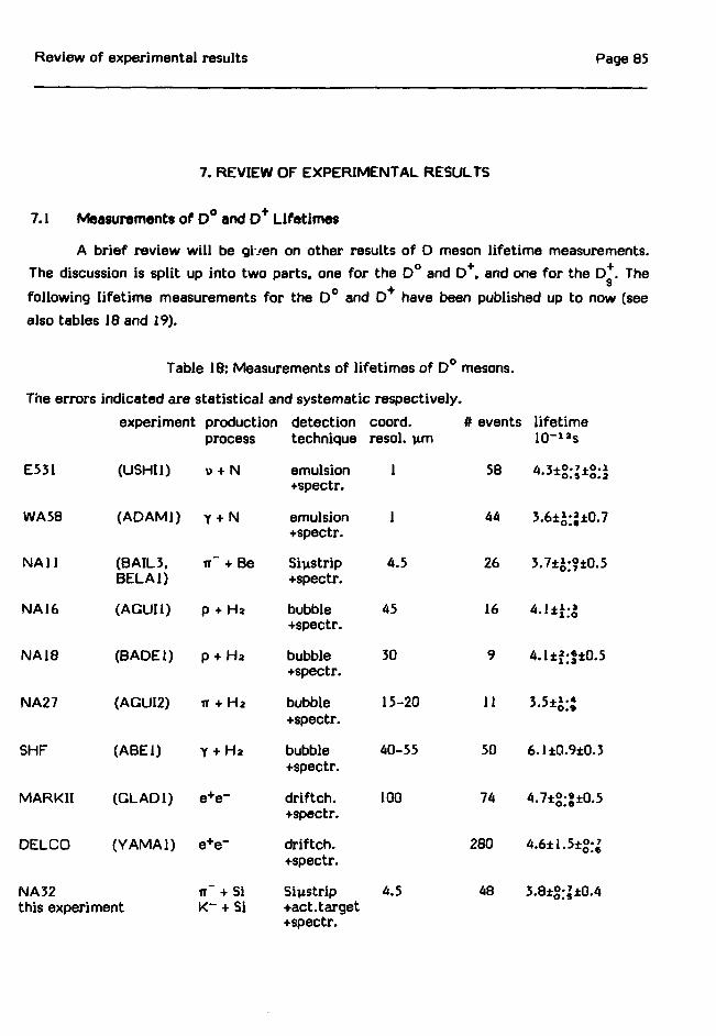
Review of experimental results Page 85
7. REVIEW OF EXPERIMENTAL RESULTS
7.1 Measurements of D° and D* Lifetimes
A brief review wil l be given on other results of O meson lifetime measurements.
The discussion is split up into two parts, one for the D° and D+, and one for the D+. The
following lifetime measurements for the 0 ° and D+ have been published up to now (see
also tables 18 and 19).
Table 18: Measurements of lifetimes of D mesons.
The errors indicated are statistical and systematic respectively.
E531
WA58
NA11
NA16
NA18
NA27
SHF
MARKII
DELCO
experiment
(USHI1)
(ADAM1)
(BAIL3.BELA1)
(AGUI1)
(BADE1)
(AGUI2)
(ABE1)
(GLAD1)
(YAMA1)
NA32this experiment
productionprocess
» + N
Y + N
w~ + Be
p + Ha
p + Ha
, + Ha
Y + Ha
e+e-
e+e~
TT~ + SiK- + Si
detectiontechnique
emulsion+spectr.
emulsion+spectr.
Siixstrip+spectr.
bubble+spectr.
bubble+spectr.
bubble+spectr.
bubble+spectr.
driftch.+spectr.
driftch.+spectr.
Siustrip+act. target+spectr.
coord,resol. v-m
1
1
4.5
45
30
15-20
40-55
100
4.5
# events
58
44
26
16
9
11
50
74
280
48
lifetime
' O.S O«3
3 . 6 * - * , ,
3.7±-+0.5
4.1±f:|±0.5
\ 5 + 1-4
6.1±0.9±0.3
4.7±g;»±0.5
4.6±1.5±g;|
3.8±g;|±0.4

Review of experimental results Page 86
Table 19: Measurements of lifetimes of D+ mescns.
The errors indicated are statistical and systematic respectively.
experiment production detection coord. # events lifetimeprocess technique resol. urn 10~13s
E531
WA58
NA1
NA11
NA16
NA18
NA27
SHF
MARKH
NA32this work
(USHI1)
(ADAM1)
(ALBI1)
(BAIL3,BELA1)
(AGUI1)
(BADE1)
(AGUI2)
(ABE1)
(GLAD1)
» + N
Y + N
Y + N
n" + Be
p + Ha
p + Ha
ir+ Ha
Y + Ha
e+e-
K-+*S1
emulsion+spectr.
emulsion+spectr.
act.target+spectr.
Siustrip+spectr.
bubble+spectr.
bubble+spectr.
bubbletspectr.
bubble+spectr.
driftch.+spectr.
Siustriptact.target+spectr.
1
1
4.5
45
30
15-20
40-55
100
4.5
28
27
98
28
15
7
23
48
23
34
l l . l± a :$
5.0±i;»il.9
9.5±J;j
10.6±|;J±1.6
8.4±1;1
6.3±*;|±1.5
9.8±»:J
8.6±1.3±g:J
8.9±|:?±1.3
9.5*-i0.4
1. E531 (USHI1): This experiment uses the wide band neutrino beam of Fermilab.
The experimental apparatus consists of an emulsion stack followed by a mag-
netic spectrometer. The scanning of the emulsion is performed by tracing the
spectrometer tracks back into the emulsion in order to find the tracks orig-
inating from primary and secondary vertices. This technique yields a higher
efficiency for finding secondary vertices than the usual volume scan in which
a search for tracks is made in a restricted volume. The reconstructed events
are distributed over many different decay modes including decay modes with
neutral secondaries which cannot be visually associated with the decay vertex.
Review of experimental results Page 87
2. WA58 (A0AM1): A stack of emulsion was placed in a photon beam in front of
the Q spectrometer at the CERN SPS. The photon energy range was 20-
70 GeV. The scanning was performed using a volume scan procedure in a
6.9 mm thick emulsion. The events were found in many different decay modes
including decay modes with neutral secondaries. The result on the D+ lifetime
from this experiment is two standard deviations lower than the world average.
5. NA16/NA27 (AGUI1.AGUI2): These experiments use different versions of the
same basic apparatus, i.e. a high resolution Ha bubble chamber (LEBC) in
front of the EHS spectrometer. The EHS spectrometer is a magnetic spec-
trometer with detectors for particle identification. The beam is a 360 GeV ir~
beam at the CERN SPS. Many different decay modes, some with neutral
particles, contribute to the final event sample.
4. NA18 (BADE1): This experiment uses a high resolution bubble chamber (BIBC)
filled with a heavy liquid (CeFe). For momentum analysis of the secondary
tracks a streamer chamber is employed. No particle identification nor ir°
detection is available. The experiment uses a 340 GeV IT' beam at the CERN
SPS. The D° signal is seen in two decay channels (Kir and K3n), the D+ signal
in one channel (Kinr).
5. SHF (ABE1): The SLAC Hybrid Facility has produced lifetime measurements
from two experiments using the same basic apparatus. The difference be-
tween the two experiments can be found in the improvements in the perfor-
mance of the apparatus. The apparatus consists of the SLAC 1 m bubble
chamber in front of a forward spectrometer. The beam is a photon beam of
20 GeV. The events are reconstructed in many different decay modes. To
compensate for missing ir°*s a special algorithm was used to obtain the
momentum of the decaying charmed meson. The lifetime results of this ex-
periment are remarkable, as their measured lifetime ratio of D° and D is
rather small, which is in particular due to one D events with a lifetime of
55«10~13s.
6. NA1 (ALBI1): This was the first experiment to employ Si detectors for a
lifetime measurement of charmed particles. The beam is a 40-150 GeV
photon beam at the CERN SPS. The experiment employs a magnetic spectro-
meter (FRAMM) and a search is made for coherent production of D mesons

Review of experimental results Page 88
on an active target. The active target consists of 40 Si detectors, 300 urnthick, which are read out layer by layer. Momentum analysis and particleidentification are performed by the downstream spectrometer. The lifetimeof the D+ mesons, which are reconstructed with the spectrometer, isdetermined in the following way. At least the first two active target layersshould have no signal, guaranteeing that the interaction takes place in thetarget. At the first occurrence of a step in signal height, indicating aninteraction in a layer, this step should correspond at least to two minimumionizing particles (m.i.p.) and persist over at least four layers. Subsequently,a second step, corresponding to 2, 4 or 6 m.i.p. extending over at least fourlayers, indicates the decay of a long lived particle. The distance corres-ponding to the number of layers in the first ionization step is a measure ofthe lifetime of the decaying particle. The decay channels selected are:D -»K+n+ff+nn ? As no connection can be made between the tracks in thespectrometer and the charge in the active target, the decay distances usedfor the lifetime determination are contaminated with D° decays, for whichcertain corrections are made.
7. NA11 (BAIL3.BELA1): The predecessor of the experiment reported on in thisthesis. The apparatus consists of a Be target placed in a 200 GeV n~ beam infront of a magnetic spectrometer. The differences with the present ex-periment (NA32) can be found in the trigger, the target and the vertex tele-scope (see also chapter 1). The events were reconstructed in the decay modesD+ -» Kirn, D° -» Kir and D° -> Kirrnr.
8. MARKII (GLAD1): the MARKH spectrometer at the PEP ring at SLAC is amagnetic spectrometer with, as a special later addition, a high resolutioncylindrical drift chamber around the beam pipe to measure the decay tracksfrom heavy flavour mesons. The D mesons for the lifetime measurement areproduced in e e~ collisions at a centre of mass energy of 29 GeV. To reduce
the background which hides the inclusive D signals, one uses the decay* *
D -» D+TT to select the events which form a peak in the D -D mass spectrum.The signal for D°, as well as the signal for D+, are observed with this method.The D° is seen in the channels K+ir and K+ir+no; the D+ is seen in the channelK+ir+ir. For these events the distance of the D decay vertex with respect tothe centre of the beam spot is measured. The lifetime is obtained from thedisplacement from zero of the distribution of these decay distances.

Review of experimental results Page 89
9. DELCO (YAMA1): The OELCO spectrometer is also situated at the PEP ringo *
at SLAC. Again the D lifetime is measured using the D decay chain to
reduce the background. To determine the lifetime, the distance of the decay
tracks of the D° are measured with respect to the beam centre (impact
parameter method). The lifetime is extracted from the displacement from
zero of the peak of this distribution.
7.2 Measurements of the D* Lifetime
The existence and mass of the D+ meson have only recently been firmly estab-
lished. The results from the e+e~ ring experiments (refs. ALBR1, ALTH1, CHEN1,
DERR1) now put its mass around 1.97 GeV. The measurement of the lifetime has only
been done by three experiments of which a summary may be found in table 20.
Table 20: Measurements of lifetimes of D+ mesons
The errors indicated are statistical and systematic respectively.
E551
NA11
HRS
NA32this work
experiment
(USHI1)
(BAIL5)
(JUNG1)
productionprocess
\> + N
n~ + Be
e+c"
K~ + Si
detectiontechnique
emulsion+spectr.
Siustrip+spectr.
driftch.+spectr.
Siustrip+act.target+spectr.
coord,resol. um
1
4.5
100
4.5
# events
6
12
17
8
lifetime
2.6*4::
3.i*S:S
3.5*f;J±0.9
3.6t}:|±0.4
1. E531 (USHI1): This experiment has published a lifetime result based on the
observation of 6 D events, decaying in three prongs, in an emulsion.
2. N A l i (BAILS): The predecessor of NA32 has published a result based on 12
events in the decay mode D -»KKir with an average lifetime of

Review of experimental results Page 90
3. HRS (JUNG1): The High Resolution Spectrometer collaboration has
measured the lifetime of a sample of 17 D events decaying in the
channel D *-»4>ff. The lifetimes were extracted from the measured de
length distribution. The average lifetime is (3.5±2'4±0.9)»10~ 13s.
7.3 Conclusions
Despite the large variations in detection techniques, each with its own statisand systematic errors, the lifetime results from most experiments are in good agreeiwith each other. Improvements on these results may be obtained by experiments viobserve large (MOO) numbers of fully reconstructed events in just a few decay chaniMoreover, for the lifetime of the D* meson one will need a good particle identificeto reject events due to misidentified D decays.
Theory and interpretation Page 91
8. COMPARISON WITH SOME MODELS
8.1 Theoretical Models
8.1.1 Introduction
In this chapter we wil l explore to what extent the results of the lifetime
measurements can be used to test two recent theoretical models. We wil l extract the
main parameters of these models, using our lifetime data . These show stil l large errors
due to the low statistics. Nevertheless some conclusions can already be drawn.
The decay of the three pseudoscalar charmed mesons (D°, D+ and D+) can bes
described with various processes. The diagrams corresponding to these processes are
shown in f ig. 8.1. The first type of diagram is the so-called spectator diagram (fig. 8.1b, c
and d) in which the c quark decays via emission of a virtual W . The other antiquark in the
meson remains unaffected by the decay, hence the name spectator quark. The second type
is the so-called W exchange diagram (fig. 8.1 e) in which both charmed quark and light
antiquark are involved and a W , originating from the decay of the c quark, is absorbed by
the light antiquark. The third type is the W annihilation diagram in which the charmed
quark and the light antiquark annihilate into a W+ (see fig. 8.If and g). The diagram in
f ig. 8f, representing the decay through W annihilation of the D+ meson, is Cabibbo
suppressed.
Naively one would expect that only the spectator diagrams have an appreciable
strength. The weak annihilation to a final state of a fermion and an antifermion is
proportional to the masses of these fermions, and hence is small due to low values of the
masses of the light quarks. This is analogous to the suppression of ir or K -»eu versus6
IT or K -»v.\> , which is known as a helicity suppression. The lifetimes in this naive quark
model would then be the same for all charmed mesons, and be related to the lifetime of
the muon which is described as well by a spectator diagram (fig. 8.1a):
with: m the mass of the muon
m the mass of the charmed quark (1.5-1.8 GeV).c
Due to the uncertainty in the value of the charm quark mass, we obtain T ~c
3.1-7.6«10~X3s. Measured D lifetimes have indeed this order of magnitude. The spectator
diagrams predict equal lifetimes for charmed particles, which is essentially

Theory and interpretation Page 92
determined by t , the lifetime of the charmed quark, and hardly influenced by the lightcquarks, i.e. :
t(D V t(D°) = T(D^) = T (8.2).
Similarly, the semileptonic branching ratios, for each lepton, for all weakly decaying
charmed states should be equal, again dominated by the semileptonic decay of the c-quark
(BRsl(c)):
BRs,(D+) « BRsI(D°) « BRsl(D^) - 8R ̂ (c) (8.3).
which in the parton model is about 20%, since one out of five charm decays leads to an
electron (muon) in the final state, as illustrated in fig. 8.2.
Both theoretical predictions are contradicted by experiment. The lifetimes show thefollowing ratios :
T(D+) /X(D°) = 2.5±0.6 (this thesis) (8.4a).
= 2.6±l.l (this thesis) (8.4b).
Measured values (8ALT1) of semiieptonic branching ratios are :
BRsl(D+) = (17.0±1.9±0.7)% (8.5).
BRsl(D°) = ( 7.5±l.l±0.4)%
The discrepancy between the predictions and the measurements of the lifetimes andbranching ratios can be attributed to either or both of the following two mechanisms.
• The influence of the strong interaction (called colour clustering) can create a
destructive interference, thus suppressing the non-leptonic decays of the D+
mesons. It is a manifestation of the Pauli principle, as two d*s are present in
the final state of Cabibbo allowed D+ decays (see fig. 8.1c). This will make
the lifetime of the D meson longer.
• A non-negligible W-exchange diagram in the D° decay and W annihilationdiagram in the D decay, implying a mechanism in the strong interaction inthe meson to counter the helicity suppression. This would decrease thelifetime of D° and D mesons.
The dominance of spectator diagrams has been used successfully by Bauer and Stech
(BAUEl) for the description of exclusive two body decays of D-mesons (see section 8.1.2).
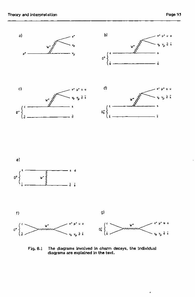
Theory and interpretation Page 93
a) b)
w*ve v^ d s
s
e)
e* | i * u u
ve V(1 a i
s
d) e* \i* u u
w * :
s d
d s
f) g)
e* (i* u u
Fig. 8.1 The diagrams involved in charm decays, the individualdiagrams are explained in the text.

Theory and interpretation Page 94
(M.2.3)
Fig. 8.2 The possible final states for the Cabibbo allowed decayof a charmed quark.
The two mechanisms responsible for the lifetime differences are discussed using a modelby Rueckl (RUEC1), describing inclusive charm decays in section 8.1.3.The measured branching ratios refered to in this chapter are summarized in table 22.
8.1.2 The decay widths of two body decays of D mesons
In order to separate the effect of the short distance strong interactions from thatof the W-exchange and annihilation diagrams, Bauer and Stech (BAUE1) have proposed thefollowing model.
It is very likely that two body decays of charmed mesons, in which the decayproducts have large momenta, are only due to spectator diagrams. They used the effectiveHamiltonian (ELLI1) for two body decays, in which they replace the V-A quark currents byhadron currents. For the non-leptonic two body decays the Hamiltonian then becomes :
H e f f = (C/V2)cos^ :(ai(ud)H(sc)H + a2(sd)H(uc)H): (8.6),
with : G the weak coupling constant,8 the Cabibbo mixing angle
(ud)H> (sc)H> (sd)H and (uc)H the hadron currents.
The real coefficients ai and a2 contain the colour exchange effects between the quarkcurrents. They are related to the QCD short distance coefficients c and c of the usualeffective quark Hamiltonian by :
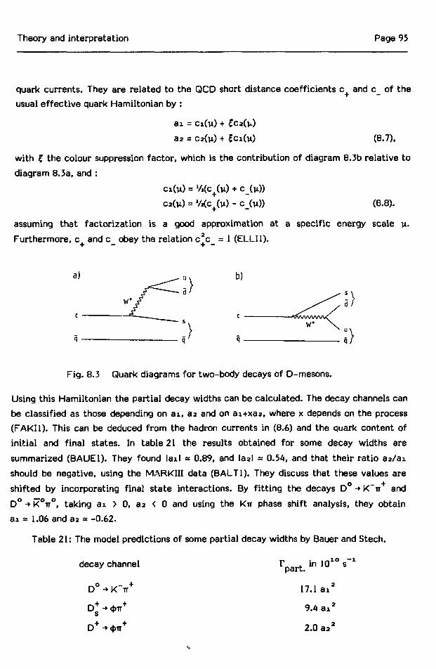
Theory and interpretation Page 95
quark currents. They are related to the QCD short distance coefficients c and c_ of the
usual effective quark Hamiltonian by :
ai =
32 = Ca(u) + fc i (u) (8.7),
with £ the colour suppression factor, which is the contribution of diagram 8.3b relative to
diagram 8.3a, and :
= V,(c+(u)
+ _ (8.8).
assuming that factorization is a good approximation at a specific energy scale u-
Furthermore, c and c obey the relation c2c_ = 1 (ELLI1).
b)
Fig. 8.3 Quark diagrams for two-body decays of D-mesons.
Using this Hamiltonian the partial decay widths can be calculated. The decay channels can
be classified as those depending on a i , aa and on ai+xa2. where x depends on the process
(FAKI1). This can be deduced from the hadron currents in (8.6) and the quark content of
initial and final states. In table 21 the results obtained for some decay widths are
summarized (BAUE1). They found lai l - 0.89, and laal = 0.54, and that their ratio aa/ai
should be negative, using the MARKIII data (BALT1). They discuss that these values are
shifted by incorporating final state interactions. By f i t t ing the decays D° -» K"TT+ and
D° -»KOTr°f taking a i > 0 , a a < 0 and using the KIT phase shift analysis, they obtain
a i - 1.06 and aa - -0.62.
Table 21: The model predictions of some partial decay widths by Bauer and Stech.
decay channel ^oart *n ^ s
D°-»K""TT+ 17.1 a i 2
D*-»<J>ir+ 9.4 a i 2
D+ •• <bir+ 2.0 aa2

Theory and interpretation Page 96
For comparison with the short distance QCD coefficients, they argue that in the
transition from quark currents to hadron currents, an additional factor of 0.9 should be
used to account for the incomplete overlap of initial and final internal meson wave
functions. In that case, they obtain a i = 1.2 and a2 = -0.72 from the MARKIII data. Using
our measurements on the lifetimes and the branching ratios of the MARKIII collaboration,
we can anew calculate the coefficients a i and as using the values for the partial widths of
table 21 from :
a i 2 = (BR[D° -» K~Tr+]/17.i»101OT(D°)) = 0.86±0.25 (8.9a)
aa 2 = (BR[D+ -> <f>Tr+]/2.CM01OT(D+)) = 0.49±0.26 (8.9b),
yielding a i = 0.93±0.14, and aa = -0.70±0.19, using the sign convention of Bauer and Stech.
Using expression 8.8 and the values of c = 0.74 and c = 1.8 at y. = 1.5 GeV obtained by
Rueckl (RUEC1), one finds c i = 1.27 and ca = -0.53. The relations (8.7) between a i , aa, c i
and ca provide two measurements of the colour suppression factor £. The average value is
£ = 0.25±0.28, which is compatible with the standard value £ = 1/3, but does not exclude a
smaller value or even £ = 0. It should be remarked that the error in £ does not contain
contributions due to the theoretical uncertainties in c i and ca (or c and c ) and the
uncertainties in the estimates of the coefficients of a2 and a2 of table 21. Moreover, a i
and a2 are obtained from two decay channels only, and not from a f i t to many channels as
inBAUEl .
We can now compare branching ratios of two body decays. Using our measurement
of t(Dg), we obtain :
BR(Dg -><t>n) = r(D+s-»<J>n)x(D+
s) = (2.9±I.3)% (8.10),
in good agreement with the value measured by the CLEO group (CHEN1) and the HRS
group (DERR1) of (3.3±1.1)% and 4.4%, respectively.
Alternatively, using the average of the measured values of BR(D* -• <J>tr), we can
derive the ratio of the lifetimes of D and D°, i .e. :s
T ( D V C ( D ° ) = (r[D°-»K'ir+]/T[D%t>ir+] • (BR[D+^t>ir+]/BR[D°-»K"ir+]) = 1.2±0.4 (8.11).s s s

Theory and interpretation Page 97
This ratio agrees well with our measured value of 0.9±0.4.
We may conclude that the analysis by Bauer and Stech gives rise to a consistent
description of the two body decay channels of D mesons via spectator diagrams.
8.1.3 The contribution of interference effects and of W exchange diagrams
In this section we will discuss a model by Rueckl (RUECl) to consider both two
body and many body charm decays, and stresses the importance of the non-spectator
processes for these decays.
Rueckl remarks that the short distance coefficients c = 0.74 and c = 1.8 at u =
1.5 GeV modify the semileptonic branching ratio of the c-quark from 20% to (RUECl):
BRgl(c) = 1 /(2+2c *+c *) =16% (8.12).
which is close to the measured value for the D+ meson of 17.0% (BALT1). However, thevalue for BR • for D° is not explained. Using the lifetimes and semileptonic branchingratio of the PDG (PDG1), we observe that the partial width for semileptonic decay of D+
and D° are nearly equal within errors at a value around F , = 20»10los~1. The deviationsfrom the total width (or lifetime) for D° and D must be due to additional non-leptonicpartial widths.
For the two mechanisms, which may resolve these discrepancies, mentioned insection 8.1.1, Rueckl (RUECl) has remarked that interference effects may increase thelifetime of the D+ meson slightly, but cannot explain e.g. the ratio T(D+) /T(D°). However,the existence of a substantial contribution of W-exchange diagrams to the decay of theD° meson is illustrated by the observation of a sizable branching ratio BR(D° -» K°<(>). Thisdecay channel can only be described by a W-exchange diagram. E.g. the ARGUScollaboration has measured this branching ratio to be (0.99±0.32±0.17)%. The helicitysuppression of the W exchange and W annihilation diagrams may be lifted by soft gluoneffects. The contribution of W exchange and W annihilation are described by theparameters P and P , which are assumed to be equal for all D-mesons. The quantitiesP* ' and P represent the product of the probability for the annihilating constituentquarks to be in a spin 1 colour singlet and a spin 1 colour octet configuration,respectively, times the spatial overlap of the wave functions of the quarks. Rueckl
(RUECl) derives the ratio p(8)/P(1J from the relationp(8)/p(l) = r t / r a ( 8 13) |
and re and n can be computed from the following lifetime ratios :
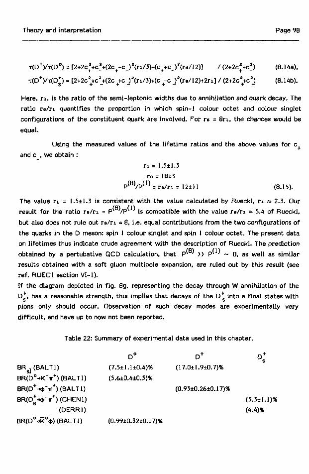
Theory and interpretation Page 98
T ( D + ) / T ( D ° ) = [2+2ca+cf+(2c+-c_)a(n/3)+(c++c_)2(r8/12)] /(2+2c%cf) (8.14a),
g) = [2+2ca++ca_+(2c ++c _)2(n/3)+(c +-c _)2(re/12)+2n] / (2+2c2
++c2_) (8.14b).
Here, n , is the ratio of the semi-leptonic widths due to annihilation and quark decay. The
ratio re/ri quantifies the proportion in which spin-1 colour octet and colour singlet
configurations of the constituent quark are involved. For re = 8n , the chances would be
equal.
Using the measured values of the lifetime ratios and the above values for c
and c , we obtain :
n = 1.5±1.3ra = 18±3
p (8) / p ( 1) _
The value rx = 1.5±1.3 is consistent with the value calculated by Rueckl, n « 2.3. Ourresult for the ratio re/ri = P̂ /P is compatible with the value TO/TX - 5.4 of Rueckl,but also does not rule out re/n = 8, i.e. equal contributions from the two configurations ofthe quarks in the D meson: spin 1 colour singlet and spin 1 colour octet. The present dataon lifetimes thus indicate crude agreement with the description of Rueckl. The predictionobtained by a pertubative QCD calculation, that P ^ >> P* ' ~ 0, as well as similarresults obtained with a soft gluon multipole expansion, are ruled out by this result (seeref. RUEC1 section VI-1).
If the diagram depicted in fig. 8g, representing the decay through W annihilation of theD , has a reasonable strength, this implies that decays of the D* into a final states withpions only should occur. Observation of such decay modes are experimentally verydifficult, and have up to now not been reported.
Table 22: Summary of experimental data used in this chapter.
BRs l(BALTl)
BR(D°-»K~Tr+)
BR(D+-xJ>~ir+)
(BALT1)
(BALT1)
(7
(5
.5±1
.6±0
D°.l±0.
.4±0.
4)%
3)%
D+
(17.0±1.9±0.7)%
(0.93±0.26±0.17)%
BR(D*-xt>"Tr+)(CHENl) (3.3±1.
(DERR1) (4.4)%
BR(Do-»K°(t>) (BALT1) (0.99±0.32±0.17)%

Theory and interpretation Page 99
8.2 Conclusions
We have applied the model of Bauer and Stech. which describes two body decays of
D mesons with a spectator mechanism, to our lifetime data. Using this model and the
measured lifetimes, i t is possible to derive BR(D -* <J>IT) well in agreement with measured
values for this branching ratio. Alternatively, the lifetime ratio T ( D * ) / T ( D ° ) predicted by
the model and using the measured value of BR(D+ -»<t>n) agrees with our value. The colour1suppression factor found is in agreement with the expected value £ = y but does not rule
out f = 0 as suggested by Bauer and Stech.
We have made a crude determination of the ratios n , re, and P /P = r e / n used
by Rueckl. The results are in agreement with the values for these ratios estimated by
Rueckl, and thus indicate that spectator and exchange/annihilation processes are of
roughly equal importance in inclusive charm decays.

Summary Page 101
SUMMARY
In this thesis an experiment is described to measure the lifetimes of pseudoscalar
charmed mesons. The experiment is located in the CERN North area and uses a negatively
charged unseparated hadron beam of 200 GeV. The experiment is carried out with a
magnetic spectrometer preceded by a beam telescope, consisting of 4 Si microstrip
detectors, an active target, consisting of 14 Si microstrip detectors, and a vertex
telescope, consisting of 7 Si microstrip detectors in 3 different strip orientations for an
accurate reconstruction of beam direction, primary and secondary vertices. The
spectrometer consists of two spectrometer magnets, 48 planes of drift chambers and 3
Cerenkov hodoscopes for the determination and identification of charged secondaries. The
lifetimes of the charmed mesons are determined by measuring the length of their flight
path, their momentum and their mass. The results, which are described in the thesis, are
based on the analysis of part of the collected data.
In chapter 2, a description is given of the spectrometer used for the measurements.
In chapter 3, the most important features of Si microstrip detectors are discussed. A
model is presented for the charge drift and diffusion in Si detectors; calculated and
measured coordinate resolutions are compared. Chapter 4 contains a description of the
trigger, the calibration procedures and the data sample collected. In particular, the
calibration of the Si detectors is described. Chapter 5 treats the track reconstruction and
event selection for this analysis. The event preselection is presented, and its acceptance
and efficiency for short lived decays is assessed. The reconstruction of tracks in the
microstrip detectors and the vertex selection with these tracks are described in detail.
In chapter 6, the mass spectra and lifetime results are presented. The lifetimes are
T(D°) = (3.8±°'7±0.4)»10~13s, T(D+ ) = (9.5±2tl±0.4)«10"13s andO.5 1.6
T(D. ) = (3.6±1'1i0.4)»10~13s. The first error is the statistical error and the secondS 1.5
error is the systematic errors (due to the selection' criteria). The production rates in the
K~ beam and in the IT" beam are found to be in the same order of magnitude within the xp
range covered. Previous experimental data on the lifetimes of charmed particles are
reviewed in chapter 7.

Summary Page 102
In the last chapter, a theoretical interpretation is presented of the measured decay
properties. The decay of each charmed meson can be described by two out of three
possible Cabibbo-allowed decay processes. The results presented on the lifetimes of D ,
D and D. show that the model of Bauer and Stech for the description of exclusive two
body decays with spectator diagrams, modified by strong interaction effects, gives a
consistent description of non-leptonic partial decay widths of these channels. The lifetime
ratios T(D )/T(D ) and T(D )/T(D ) are in agreement with estimates of Rueckl on the
relative contribution of the semi-leptonic decay widths to quark decay and W
exchange/W-annihilation. indicating that W exchange/W annihilation is an equally
important decay mechanism.

Samenvatting Page 103
SAMENVATTING
In dit proefschrift wordt een experiment beschreven, waarin de levensduren van de
pseudoskalaire mesonen worden gemeten, die het vierde quark, charm, beva en. De
experimentele opstelling bevindt zich in de Noordhal van CERN. Met behulp van het
CERN Super Proton Synchrotron (SPS) wordt een bundel negatief geladen hadronen met
een impuls van 200 GeV naar het experiment gezonden. De experimentele opstelling is
samengesteld uit een magnetische spektrometer, voorafgegaan, in volgorde door: de
bundeldetektoren, de aktieve trefplaten en een vertex teleskoop. De bundel wordt
waargenomen met vier Si mikrostrip detektoren met drie verschillende oriëntaties van de
detektiestroken. De aktieve trefplaten, waarmee de bundeldeeltjes kunnen botsen, worden
gevormd door 14 dicht opeen geplaatste Si mikrostrip detektoren. De ionisatie
veroorzaakt door de reaktieprodukten kan met deze detektoren worden waargenomen. De
in de botsing of door verval gevormde deeltjes worden gedetekteerd met de vertex
teleskoop, met 7 Si mikrostrip detektoren, eveneens met drie verschillende oriëntaties van
de detektiestroken. De impuls en identiteit van de gevormde deeltjes worden gemeten met
de spektrometer, welke de volgende elementen bevat: twee spektrometer magneten, 48
driftkamer vlakken en 3 veelcellige Cerenkov tellers. De levensduur van een charm meson
wordt bepaald door de afstand tussen de produktievertex an de vervals vertex, alsmede
door de massa en de impuls. De in dit proefschrift gepresenteerde resultaten zijn
gebaseerd op de analyse van een deel van het totale gegevensbestand.
In hoofdstuk 2 wordt een beschrijving gegeven van de experimentele opstelling.
Hoofdstuk 3 bevat enkele belangrijke eigenschappen van Si mikrostrip detektoren. De drift
en diffusie van de in de Si detektoren door de deeltjes vrijgemaakte ladingen worden in
een model beschreven. Het op deze wijze berekende oplossend vermogen wordt vergeleken
met de gemeten waarden. Hoofdstuk 4 bevat een beschrijving van de direkte
instrumentele selektie van gebeurtenissen, van de kalibratie van de detektoren en van het
verzamelde gegevensbestand. In hoofdstuk 5 worden de rekonstruktie en de selektie van
gebeurtenissen door het analyseprogramma behandeld. Aan het begin van de rekonstruktie
worden de gebeurtenissen voorgeselekteerd. Een beschrijving van deze voorselektie wordt
gegeven en de doeltreffendheid ervan voor gebeurtenissen met een kortlevend verval
wordt geschat. De rekonstruktie van de sporen in de vertex teleskoop en de selektie van
de gerekonstrueerde vertices worden in detail behandeld. De berekende levensduren van
de charm mesonen worden in hoofdstuk 6 gepresenteerd. De levensduren

Samenvatting Page 104
zijn t(Do)=(3.8±o'7±0.4)«10" ias T ( D + ) = ( 9 . 5 ± S - 1 ± 0 . 4 ) . 1 0 " 1 3 S enO.5 1.6
T(D )= (3 .6± X - 1 ±0 .4 )»10~ 1 3 S. De aangegeven fouten zijn respektievelijk de statistischeS 1 «5
en de systematisch fout (ten gevolge van de selektie procedure). Uit de geobserveerde
signalen wordt gekonkludeerd dat de charm mesonen in trSi en KSi wisselwerkingen, binnen
de fout, en in het door de spektrometer bestreken x p interval, in gelijke mate
geproduceerd worden. Hoofdstuk 7 bevat een korte samenvatting var.' deze levensduren
gemeten in andere experimenten. Het laatste hoofdstuk bespreekt twee theoretische
beschrijvingen van de vervalseigenschappen van charm mesonen. Het verval van elk van de
drie mesonen kan beschreven worden door twee van drie mogelijke vervals processen. De
modelbeschrijving van Bauer en Stech voor de vevalskanalen van charm mesonen naar
twee deeltjes vormt, als de levensduurresultaten gebruikt worden, een konsistent beeld
van de vervalsbreedten van deze niet leptonische vervalskanalen. De schattingen van
Rueckl ten aanzien van de bijdrage van de semi-leptonische vervalsbreedten tot het quark
verval en de W annihilatie/W uitwisseling zijn in overeenstemming met de geobserveerde
verhoudingen van de levensduren T ( D + ) / T ( D ° ) en T ( D + ) / T ( D + ) . Dit laatste toont aan dat W
annihilatie en W uitwisseling processen zijn die in sterkte vergelijkbaar zijn met het
toeschouwer proces.

Acknowledgements Page 105
ACKNOWLEDGEMENTS
At this place I have the pleasure to thank everybody who had a constructivecontribution to this thesis.
I thank the members of the ACCMOR collaboration for the pleasant cooperation. Ithas been a very positive experience and a great pleasure to work at CERN in aninternational group. I acknowledge each individual contribution by the group memberswithout going to the sheer impossible task of listing them.
I make an exception for Kees Daum to thank him for his constant support andenthusiasm. Most of the results in this thesis were product of our cooperation, acooperation I experienced as very pleasant and instructive.
I thank Prof. Kluyver , my promotor, for carefully reading the manuscript.Carol Ponting can type a thesis in 4 days, something I thought impossible until I
actually saw it happen.Finally I would like to thank Lucie for her support throughout all these years.

References Page 107
REFERENCES
ABE1 K. Abe et ah, Phys. Rev. D 33 (1984) 1.
ADAMI M. Adamovich et al., CERN-EP/86-77 June 1986, submitted to Phys. Lett. B.
AGUI1 M. Aguilar-Benitez et al.. Phys. Lett. 122B (1983) 312.
AGUI2 M. Aguilar-Benitez et al., CERN-EP/85-130, submitted to Z. Phys. C.
ALBI1 E. Albini et al.. Phys. Lett. 110B (1982) 339.
ALBR1 H. Albrecht et al., Phys. Lett. 153B (1985) 343.
ALBR2 H. Albrecht et al., Phys. Lett. 158B (1985) 525.
ALTH1 M. Althoff et al., Phys. Lett. 136B (1984) 130.
BADE 1 A. Badertscher et al., Phys. Lett. 123B (1983) 471.
BAIL1 R. Bailey et al., Nucl. Instrum. and Meth. 226 (1984) 56-58.
BAIL2 R. Bailey et al., proposal NA32, CERN/SPSC/82-57, SPSC/P180.
BAIL3 R. Bailey et al., Z. Phys. C 28 (1985) 357-363.
BAIL4 R. Bailey et al., Z. Phys. C 30 (1986) 51-63.
BAILS R. Bailey et al.. Phys. Lett. 139B (1984) 320, Contr. to Int. Europhysics Conf. onHigh Energy Physics, Bari 1985.
BAIL6 R. Bailey et al., Phys. Lett. 132B (1983) 230.
BALT1 R. Baltrusaitis et al., Phys. Rev. Lett. 54 (1985) 1976;R. Baltrusaitis et al.. Phys. Rev. Lett. 55 (1985) 150;R. Baltrusaitis et al., Phys. Rev. Lett. 56 (1986) 2141.
BAUE1 M. Bauer & B. Stech. Phys. Lett. 152B (1985) 380;Proc. Moriond Workshop on Flavour Mixing and C.P. Violation, La Plagne 1985,p. 151.
BEBE1 C. Bebek et al., Cleo-86-2 CLNS-86/715.
BELA1 E. Belau, Ph.D. thesis Ludwig-Maximilians Universitat, Miinchen 1985;MPI-PAE/Exp. El. 151, June 1985.
BELA2 E. Belau et al.. Nucl. Instr. and Meth. 214 (1983) 253-260.
BELA3 E. Belau et al.. Contr. to Int. Conf. on Hadron Spectr., Maryland, April 1985.

References Page 108
BIGI1 I. Bigi. PITHA 85/14. August 1985.
BLAN1 G. Blanar et al., proposal NA11, CERN/SPSC/78-14. SPSC/P95.
8LUN1 O. Blunck & S. Leisegang. Z. Phys. C 128 (1950) 500.
CASO1 C. Caso & M. Touboul, submitted to La Rivista del Nuovo Cimento,CERN-EP/85-176.
CHAR1 G. Charpak & F, Sauli. CRRN-EP/84-35.
CHEN1 A. Chen et al., Phys. Rev. Lett. 51 (1983) 634.
DAUM1 C. Daum et al., Much Instr. and Meth. 176 (1980) 119-127.
DERR1 M. Derrick et al, Phys. Rev. Lett. 54 (1985) 2568.
DIJK1 H. Dijkstra. Ph.D. thesis. Universiteit van Amsterdam, 1985.
EADY1 W. Eady, D. Drijard, F. James, M. Roos and B. Sadoulet, Statistical methods inexperimental physics. North Holland, 1971, section 9.3.
ELLI1 J. Ellis et al., Nucl. Phys. B100 (1975) 313
ENGL1 J. England et al., Nucl. Instr. and Meth. 185 (1981) 43-47.
FAKI1 D. Fakirov and B. Stech, Nucl. Phys. B133 (1978) 315-326.
FANO1 U. Fano, Ann. Rev. Nucl. Sci. 13 (1963) 1.
FLAM1 V. Flamino et al., CERN-HERA 79-01.
GLAD1 L. Gladney, Ph.D. thesis, Stanford 1985.
HALL1 G. Hall, IC/HENP/83-1.
HANC1 S. Hancock et al.. CERN DD/83/14, EP/83-76.
HANC2 S. Hancock et al., CERN DD/83/20, EP/83-138.
HAUS1 J. Hauser, Ph.D. thesis. Cal. Inst. of Techn., 1985 (unpublished).
HEIJ1 E. Heijne, Ph.D. thesis, Universiteit van Amsterdam, 1983; CERN-EF/83-06.
HYAM1 B. Hyams et al., Nucl. Instr. and Meth. 205 (1983) 99-105.
JUNG1 C. Jung et al.. Phys. Rev. Lett. 56 (1986) 1775.
KOLB1 K. Kolbig & B. Schorr, Asymptotic expansion for the Landau density anddistribution functions, CERN.
LAND1 L. Landau, J. of Phys. (USSR) 8 (1944) 201.
References Page 109
NEUG1 E. Neugebauer, Ph.D. thesis Ludwig-Maximilians Universitat, München 1984;MPI-PAE/Exp. El. 152. November 1984.
PDG1 Particle Data group, Rev. Mod. Phys., vol. 56, no. 2, part 2, April 1984.
PETE1 S. Peters, Ph.D. thesis, Universiteit van Amsterdam, 1980.
RANCI P. Rancoita & A. Seidman, La Revista del Nuovo Cimento, No. 7 (1982).
REAY1 N. Reay, Proc. Int. Lepton/Photon Symp., Cornell Univ. 1983. p. 244.
REAY2 N. Reay, Int. Conf. on Phys. in Collision. Como 1983.
ROSSI B. Rossi, High energy particles, 1952.
RUEC1 R. Rueckl. Habilitationsschrift. Univ. Munich 1983.
SHUL1 P. Shulek et al., Soviet J. Nucl. Phys. 4 (1967) 400.
SPIE1 W. Spierenburg, Ph.D. thesis, Universiteit van Amsterdam, 1983.
SZE1 Sze, Physics of Semiconductor Devices, 1981.
USHI1 N. Ushida et al.. Phys. Rev. Lett. 56 (1986) 1767; Phys. Rev. Lett. 56 (1986)1771.
VAVI1 P. Vavilov, Soviet Phys. JETP 5 (1957) 749.
YAMA1 H. Yamamoto et al., SLAC-PUB-3628 (1985). submitted to Phys. Rev. D.