Eliciting ambiguity aversion in unknown and in compound lotteries: a smooth ambiguity model...

Theory Dec.DOI 10.1007/s11238-013-9406-z

Eliciting ambiguity aversion in unknownand in compound lotteries: a smooth ambiguitymodel experimental study

Giuseppe Attanasi · Christian Gollier ·Aldo Montesano · Noemi Pace

© Springer Science+Business Media New York 2014

Abstract Coherent-ambiguity aversion is defined within the (Klibanoff et al., Econo-metrica 73:1849–1892, 2005) smooth-ambiguity model (henceforth KMM) as thecombination of choice-ambiguity and value-ambiguity aversion. Five ambiguous deci-sion tasks are analyzed theoretically, where an individual faces two-stage lotteries withbinomial, uniform, or unknown second-order probabilities. Theoretical predictions arethen tested through a 10-task experiment. In (unambiguous) tasks 1–5, risk aversion iselicited through both a portfolio choice method and a BDM mechanism. In (ambigu-ous) tasks 6–10, choice-ambiguity aversion is elicited through the portfolio choicemethod, while value-ambiguity aversion comes about through the BDM mechanism.The behavior of over 75 % of classified subjects is in line with the KMM model in alltasks 6–10, independent of their degree of risk aversion. Furthermore, the percentageof coherent-ambiguity-averse subjects is lower in the binomial than in the uniformand in the unknown treatments, with only the latter difference being significant. Themost part of coherent-ambiguity-loving subjects show a high risk aversion.

Keywords Coherent-ambiguity aversion · Value-ambiguity aversion ·Choice-ambiguity aversion · Smooth ambiguity model · Binomial distribution ·Uniform distribution · Unknown urn

JEL Classification D81 · D83 · C91

G. Attanasi (B)University of Strasbourg (BETA), Strasbourg, Francee-mail: [email protected]

C. GollierToulouse School of Economics, Toulouse, France

A. MontesanoBocconi University, Milan, Italy

N. PaceUniversity Ca’ Foscari of Venice, Venice, Italy

123

G. Attanasi et al.

1 Introduction

This paper proposes a series of ten experimental decision tasks involving two-outcomelottery choices. Five of these tasks are aimed at eliciting a subject’s attitude toward risk,and the other five are designed to study her attitude toward ambiguity. Specific theo-retical predictions about a subject’s behavior in the latter decision tasks are obtained,by relying on the Klibanoff et al. (2005) smooth ambiguity model (henceforth KMM).The paper has three main goals.

The first objective is to propose a simple experimental method able to makeKMM operational in individual decision tasks. To this purpose, the experimen-tal environment is explicitly designed in order to match KMM intuition of mod-eling ambiguity through two-stage lotteries. In such an environment, two dif-ferent operational definitions of ambiguity aversion are provided. The first one,namely value-ambiguity attitude, is based on Becker and Brownson (1964) ideathat “individuals are willing to pay money to avoid actions involving ambigu-ity” (p. 5).1 A value-ambiguity-averse subject values an ambiguous lottery lessthan its unambiguous equivalent with the same mean probabilities. In the KMMmodel, this is true if the subject’s φ function is concave. The second defini-tion, namely choice-ambiguity attitude, relies on Gollier (2012) intuition that moreambiguity-averse subjects should have a smaller demand for a risky asset whosedistribution of returns is ambiguous. It should be noted that a portfolio contain-ing a larger share invested in the risky asset may be seen as a two-stage lot-tery where second-order objective probabilities are more dispersed. In the KMMframework, Gollier (2012) has shown that an ambiguity-averse subject might havea larger demand for the risky asset than another ambiguity-neutral subject withthe same risk aversion, thereby deducting that a value-ambiguity averse subject isnot necessarily choice-ambiguity averse. On the other hand, Gollier (2012) pro-vides a set of sufficient conditions on the structure of the two-stage uncertaintyto re-establish the link between the concavity of φ and choice-ambiguity aversion.Given that one of these sufficient conditions is satisfied in our experimental deci-sion tasks, an equivalence between value-ambiguity attitude and choice-ambiguityattitude is expected, and defined as coherent-ambiguity attitude within the KMMframework.

The second objective of the paper is to check behavioral predictions obtained withinthe KMM model in the five decision tasks aimed at studying a subject’s ambiguity atti-tude. In all ambiguous decision tasks, the subject always faces the same two (second-stage) lottery outcomes. Thus, within the same treatment, each ambiguous task differsfrom the next one only because of the level of ambiguity of the decision setting and/or

1 After Becker and Brownson (1964), the idea that information which reduces ambiguity has a positivevalue for ambiguity-averse subjects has been clearly stated within different decision-theoretic models, e.g.,Quiggin (2007), using Machina (2004) concept of almost-objective acts; Attanasi and Montesano (2012),relying on the Choquet expected utility model. Moreover, focusing on a specific adaptation of KMM, Snow(2010) has proved that the value of information that resolves ambiguity increases with greater ambiguityand with greater ambiguity aversion. Attanasi and Montesano (2012) have obtained similar results withinthe Choquet model.

123

Eliciting ambiguity aversion in unknown and in compound lotteries

because of a first-degree stochastic improvement in the distribution of second-orderprobabilities. In particular, these tasks are designed in such a way that once a sub-ject has been classified as coherent-ambiguity-averse, coherent-ambiguity-neutral, orcoherent-ambiguity-loving, the sign of the variation of her certainty equivalent fromone task to the next one should depend only on this classification. Therefore, this signshould be predicted directly by the “sign” of her attitude toward ambiguity as deter-mined within KMM. This means that, by construction, the verification of our maintheoretical predictions in these tasks should be independent of the subject’s degree ofrisk aversion as elicited in the five unambiguous tasks. Finding an effect of risk attitudeover the behavioral verification of our theoretical hints would raise some doubts onthe use of KMM as reference model for the tasks proposed in our experiment. Theelicitation of risk attitude is also important in order to empirically ascertain whether itinfluences the “sign” of the ambiguity attitude, i.e., which one of the three ambiguityattitudes (aversion, neutrality, or proneness) the subject will show. Our design is alsoaimed at finding whether this “sign” may depend on the riskiness of the second-stagelottery, i.e., on the spread of the difference of its two outcomes. In order to be con-sistent in the elicitation of risk attitude and of ambiguity attitude, the same pair ofinstruments are used for both attitudes. In particular, risk attitude is elicited throughboth a portfolio choice method and a Becker et al. (1964) mechanism (henceforthBDM). Correspondingly, choice-ambiguity aversion is established through the firstmethod and value-ambiguity aversion through the second one. The combination ofthe two instruments has a twofold role. For risk attitude, it allows to check that bothinstruments lead to similar subjects’ orderings. For ambiguity attitude, it affords toelicit separately the two features of (coherent)-ambiguity attitude introduced abovewithin KMM. Concerning risk attitude, once the correlation between the two risk-aversion orderings has been verified, the results of the portfolio choice method arerelied upon: this has the advantage of imposing some theoretically derived constraintswhich allow to check whether the subject’s selected portfolio is compatible with aconstant absolute and/or a constant relative risk aversion specification. Concerningambiguity attitude, throughout the paper we consider as “classified subjects” onlythose who provide coherent answers under the two instruments. This provides a ratio-nale for the term “coherent” to identify the kind of ambiguity attitude studied in thispaper.

The third objective of the paper is to analyze how subjects’ decisions under ambi-guity react to different distributions of second-order probabilities. The experimentconsists of three treatments, according to a between-subject design. The five unam-biguous tasks do not vary among treatments, while the ambiguous tasks are differentfor each treatment, in the way in which uncertainty over the composition of the urnsused to perform them is generated. More precisely, the first of these tasks relies on a10-ball small urn containing white and orange balls; subjects are not told its composi-tion. In all treatments said composition is generated through a random draw from a bigurn, introduced in order to mimic KMM two-stage lottery approach. In treatment 1,the composition of the 10-ball small urn is determined through a Bernoullian processover a 50-white-50-orange balls big urn, thereby leading to a binomial distributionof second-order probabilities. In treatment 2, subjects are shown that second-orderprobabilities over the composition of the 10-ball small urn are uniformly distributed.

123

G. Attanasi et al.

In treatment 3, subjects have no information about the composition of the 10-ball smallurn, although—to make it comparable to treatment 1—ambiguity is generated througha two-stage lottery procedure similar to the one of the binomial treatment, though withno information provided about the composition of the big urn. The uniform distributionof the second-order probabilities in treatment 2 is clearly a mean-preserving spreadof the binomial distribution obtained in treatment 1. Treatment 3 is intrinsically moreambiguous than treatment 1. Therefore, under ambiguity aversion, it is expected thatin the first ambiguous task of both the uniform and the unknown treatment, the subjectwill assign a lower value to the ambiguous lottery than in the corresponding task of thebinomial treatment. This should also happen in the remaining ambiguous tasks, pro-vided, once the 10-ball small urn is generated, the way its composition is “modified” inorder to vary the level of ambiguity and the distribution of second-order probabilitiesis the same in each treatment. Although our design is not within-subject, the above-stated predictions can be checked by comparing the distribution of subjects’ decisionsin the ambiguous tasks of the three treatments. This treatment comparison would holdonly under the assumption that the distribution of subjects’ degree of risk aversiondoes not differ among the three treatments. This is an additional reason for elicitingrisk attitude before looking at subjects’ decisions in the ambiguous tasks.

The rest of the article is structured as follows. Section 2 describes the experimentaldesign, by highlighting the motivations behind the ten decision tasks. Section 3 ana-lyzes the five decision tasks under ambiguity and presents the main theoretical results.Section 4 presents the results of our experiment. In Sect. 5, the experimental designand results are discussed within the experimental literature on ambiguity aversion.Section 6 concludes.

2 Experimental design

Experimental subjects were graduate students in Economics of the Toulouse School ofEconomics (TSE). Computerized sessions were conducted at the Laboratory of Exper-imental Economics of TSE. A total of 105 (42 women, 63 men, average age = 23.70)participated in our experiment, with each subject participating only once. Averageearnings were approximately C= 20.50 per subject, including a C= 5.00 show-up fee. Theexperiment was programed using the z-Tree software (Fischbacher 2007) and subjectswere seated in isolated cubicles in front of computer terminals. Three treatments wererun through a between-subject design, with the same number of subjects (N = 35)participating in each treatment. The number of subjects in each session varied from aminimum of 9 to a maximum of 18.2

The experiment consists of ten decision tasks per treatment.3 At the beginning ofthe experiment, participants were told the number of tasks. However, instructions forevery new task were given and read aloud only prior to that task. After instructions

2 For treatment 1, two sessions were run, respectively, with 17 and 18 students. Treatment 2 had threesessions, respectively, with 16, 10, and 9 students. Treatment 3 also had three sessions, respectively, with12, 10, and 13 subjects.3 Experimental instructions are available upon request.

123


Table 1 Main features of the ten decision tasks

All Treatments Treatment 1 Treatment 2 Treatment 3Task Elicitation Method Features of the lotteries Task1-4 Portfolio Choice 1-4 5 BDM mechanism

Simple Lottery 5

6-9 BDM mechanism 6-9 10 Portfolio Choice

Binomial Compound Lottery

Uniform Compound Lottery

Unknown (Compound) Lottery 10

Table 2 Portfolio choice intasks 1–4: pairs of lotteryoutcomes

Task t = 1 Task t = 2 Task t = 3 Task t = 4

x j1 x j

1 x j2 x j

2 x j3 x j

3 x j4 x j

4

Lottery j = A 12 6 11 6 20 14 19 14

Lottery j = B 16 4 14 4 24 12 22 12

Lottery j = C 20 2 17 2 28 10 28 8

Lottery j = D 24 0 20 0 32 8 34 4

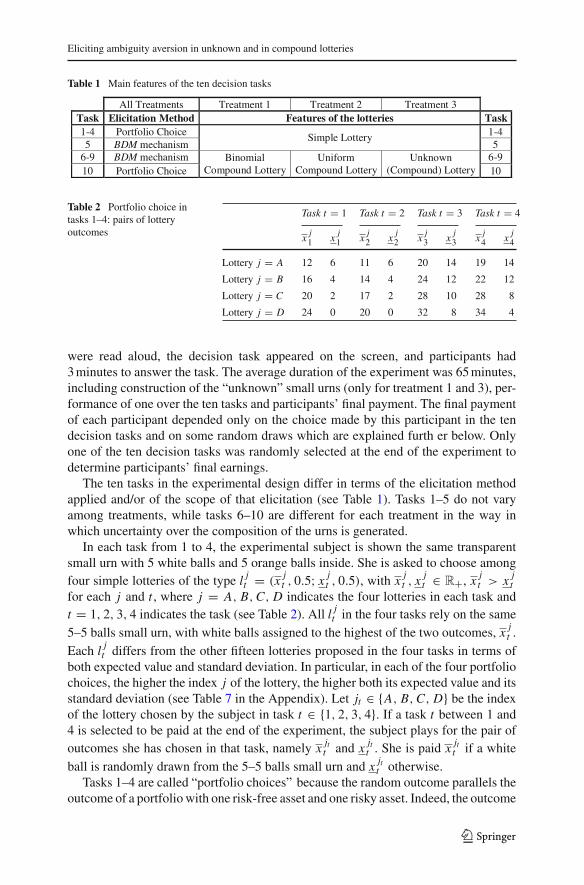
were read aloud, the decision task appeared on the screen, and participants had3 minutes to answer the task. The average duration of the experiment was 65 minutes,including construction of the “unknown” small urns (only for treatment 1 and 3), per-formance of one over the ten tasks and participants’ final payment. The final paymentof each participant depended only on the choice made by this participant in the tendecision tasks and on some random draws which are explained furth er below. Onlyone of the ten decision tasks was randomly selected at the end of the experiment todetermine participants’ final earnings.

The ten tasks in the experimental design differ in terms of the elicitation methodapplied and/or of the scope of that elicitation (see Table 1). Tasks 1–5 do not varyamong treatments, while tasks 6–10 are different for each treatment in the way inwhich uncertainty over the composition of the urns is generated.

In each task from 1 to 4, the experimental subject is shown the same transparentsmall urn with 5 white balls and 5 orange balls inside. She is asked to choose amongfour simple lotteries of the type l j

t = (x jt , 0.5; x j

t , 0.5), with x jt , x j

t ∈ R+, x jt > x j

tfor each j and t , where j = A, B, C, D indicates the four lotteries in each task andt = 1, 2, 3, 4 indicates the task (see Table 2). All l j

t in the four tasks rely on the same5–5 balls small urn, with white balls assigned to the highest of the two outcomes, x j

t .Each l j

t differs from the other fifteen lotteries proposed in the four tasks in terms ofboth expected value and standard deviation. In particular, in each of the four portfoliochoices, the higher the index j of the lottery, the higher both its expected value and itsstandard deviation (see Table 7 in the Appendix). Let jt ∈ {A, B, C, D} be the indexof the lottery chosen by the subject in task t ∈ {1, 2, 3, 4}. If a task t between 1 and4 is selected to be paid at the end of the experiment, the subject plays for the pair ofoutcomes she has chosen in that task, namely x jt

t and x jtt . She is paid x jt

t if a whiteball is randomly drawn from the 5–5 balls small urn and x jt

t otherwise.Tasks 1–4 are called “portfolio choices” because the random outcome parallels the

outcome of a portfolio with one risk-free asset and one risky asset. Indeed, the outcome

123

G. Attanasi et al.

Table 3 Reinterpretation of thelottery choices into portfoliochoices for tasks 1–4

wt yt yt

αj=At α

j=Bt α

j=Ct α

j=Dt

Task t = 1 8 4 −2 1 2 3 4

Task t = 2 8 3 −2 1 2 3 4

Task t = 3 16 4 −2 1 2 3 4

Task t = 4 16 3 −2 1 2 4 6

l j tt of choice j in task t can be written as (wt −α

jt )(1+r f )+α

jt (1+ yt ), where wt can

be interpreted as the initial wealth in task t , and αjt is the euro investment in the risky

asset: r f is the risk-free rate that is always normalized to 0, and yt is the return of therisky asset in task t. The return of the risky asset can take two possible values yt andy

twith equal probabilities. In Table 3, the portfolio contexts and portfolio choices in

the four tasks are reinterpreted.In task 5, the subject is assigned the same pair of lottery outcomes she has chosen

in task 4, namely x j44 and x j4

4 . The same 5–5 balls small urn of tasks 1–4 is used, with

white balls again assigned to x j44 , in order to build the lottery l j4

4 = (x j44 , 0.5; x j4

4 , 0.5).Therefore, the subject’s “initial endowment” in task 5 is her preferred lottery in task4. In task 5, the subject has the possibility to sell l j4

4 through a BDM mechanism.4

She is asked to state the smallest price at which she is willing to sell l j44 , by setting a

price between x j44 and x j4

4 . This reservation price should provide an approximation of

the subject’s certainty equivalent of l j44 . The BDM mechanism here used is very close

to the one implemented by Halevy (2007). Differently from Halevy (2007), however,there are four lotteries l j

4 for which a subject may state her reservation price andthe set of possible “buying/selling prices” is discrete. The discreteness of the set ofpossible “buying/selling prices” is due to the fact that the BDM mechanism used hereis implemented through real tools, as every instrument in our experimental design.Indeed, as will be shown below, in this experiment none of the random draws fromany urn is computerized. In the same spirit of concreteness, for each lottery l j4

4 chosenin task 4, there is a different envelope containing a finite set of numbered tickets.A random draw of a numbered ticket from this envelope gives the buying price forlottery l j4

4 .5

4 Given that the subject has to set the price at which to sell a random “initial endowment”, she is assigneda lottery that she has just declared to prefer among four possible lotteries (task 4). Therefore, her “initialendowment” in task 5 (and, as will be shown, in tasks 6–9) depends on the choice made in task 4, althoughthe subject does not know this in task 4.5 More specifically, there are four different envelopes, labeled respectively with letter A, B, C and D, i.e.,one for each lottery available in task 4. Each of these envelopes contains eleven different numbered tickets.The distance between two subsequent numbers on the tickets in an envelope is the same, so as to have the

same number of tickets in each envelope, with the lowest numbered ticket being equal to x j4 and the highest

being equal to x j4. In particular, the eleven tickets inside envelope A are 14, 14.5, . . . , 18.5, 19 ; those inside

envelope B are 12, 13, . . . , 21, 22; those inside envelope C are 8, 10, . . . , 26, 28; those inside envelope D

are 4, 7, . . . , 31, 34. The eleven tickets in envelope j represent the set of possible prices of lottery lj44 ,

with j = A, B, C, D. A ticket is randomly drawn from each envelope. The ticket drawn from envelope jdetermines the random “buying price” for lottery j . Then, without knowing this price, the subject states

123


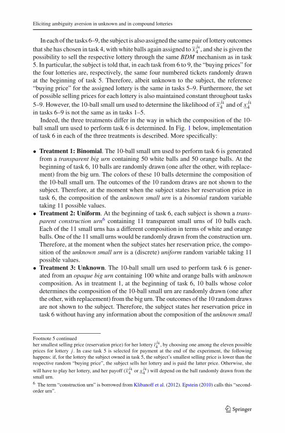
In each of the tasks 6–9, the subject is also assigned the same pair of lottery outcomesthat she has chosen in task 4, with white balls again assigned to x j4

4 , and she is given thepossibility to sell the respective lottery through the same BDM mechanism as in task5. In particular, the subject is told that, in each task from 6 to 9, the “buying prices” forthe four lotteries are, respectively, the same four numbered tickets randomly drawnat the beginning of task 5. Therefore, albeit unknown to the subject, the reference“buying price” for the assigned lottery is the same in tasks 5–9. Furthermore, the setof possible selling prices for each lottery is also maintained constant throughout tasks5–9. However, the 10-ball small urn used to determine the likelihood of x j4

4 and of x j44

in tasks 6–9 is not the same as in tasks 1–5.Indeed, the three treatments differ in the way in which the composition of the 10-

ball small urn used to perform task 6 is determined. In Fig. 1 below, implementationof task 6 in each of the three treatments is described. More specifically:

• Treatment 1: Binomial. The 10-ball small urn used to perform task 6 is generatedfrom a transparent big urn containing 50 white balls and 50 orange balls. At thebeginning of task 6, 10 balls are randomly drawn (one after the other, with replace-ment) from the big urn. The colors of these 10 balls determine the composition ofthe 10-ball small urn. The outcomes of the 10 random draws are not shown to thesubject. Therefore, at the moment when the subject states her reservation price intask 6, the composition of the unknown small urn is a binomial random variabletaking 11 possible values.

• Treatment 2: Uniform. At the beginning of task 6, each subject is shown a trans-parent construction urn6 containing 11 transparent small urns of 10 balls each.Each of the 11 small urns has a different composition in terms of white and orangeballs. One of the 11 small urns would be randomly drawn from the construction urn.Therefore, at the moment when the subject states her reservation price, the compo-sition of the unknown small urn is a (discrete) uniform random variable taking 11possible values.

• Treatment 3: Unknown. The 10-ball small urn used to perform task 6 is gener-ated from an opaque big urn containing 100 white and orange balls with unknowncomposition. As in treatment 1, at the beginning of task 6, 10 balls whose colordetermines the composition of the 10-ball small urn are randomly drawn (one afterthe other, with replacement) from the big urn. The outcomes of the 10 random drawsare not shown to the subject. Therefore, the subject states her reservation price intask 6 without having any information about the composition of the unknown small

Footnote 5 continuedher smallest selling price (reservation price) for her lottery l

j44 , by choosing one among the eleven possible

prices for lottery j . In case task 5 is selected for payment at the end of the experiment, the followinghappens: if, for the lottery the subject owned in task 5, the subject’s smallest selling price is lower than therespective random “buying price”, the subject sells her lottery and is paid the latter price. Otherwise, she

will have to play her lottery, and her payoff (x j44 or x

j44 ) will depend on the ball randomly drawn from the

small urn.6 The term “construction urn” is borrowed from Klibanoff et al. (2012). Epstein (2010) calls this “second-order urn”.

123

G. Attanasi et al.

100 balls

white or orange

50 white balls

50 orange balls Random draw of 10 balls

Random draw of one ball

10 balls

w or o

Payment Subject’s Choice

Random draw of 10 balls


10 balls

w or o


8 w - 2 o

6 w - 4 o7 w - 3 o

5 w - 5 o

1 w - 9 o0 w - 10 o

2 w - 8 o

3 w - 7 o

4 w - 6 o

10 w - 0 o

9 w - 1 oRandom draw of 1 small urn



# w - # o

Treat 1:

Binomial

Treat 2:

Uniform

Treat 3:

Unknown

If Task 6 is selected at the end of the experiment:



Fig. 1 Implementation of task 6 in each treatment

urn. The reason why ambiguity is generated through a two-stage lottery is to makethis treatment comparable to treatment 1.

Tasks 7–9 involve the elimination of some possible compositions of the 10-ballunknown small urn used to perform task 6. At the beginning of task 7, the subject istold that, if this task were to be performed at the end of the experiment, the number ofwhite balls in the unknown small urn would be between 3 and 7 (and so the numberof orange balls). This would be implemented in the following way. In treatment 1 andtreatment 3, 6 balls will be taken out of the unknown small urn constructed at thebeginning of task 6 and replaced with 3 white balls and 3 orange balls. In treatment2, six transparent small urns (the three with less than 3 white balls and the three withless than 3 orange balls) will be taken out of the transparent construction urn. Task 8(9) differs from task 7 only for the fact that in the unknown small urn, the number ofwhite (orange) balls will be between 3 and 10.

In each of the tasks 6–9 the subject, besides stating her reservation price for thelottery resulting from the corresponding unknown small urn, is also asked to guess thenumber of white balls in that urn. In case a task from 6 to 9 is randomly selected to beperformed at the end of the experiment, the subject is paid an additional C= 5.00 if herguess of the number of white balls in the unknown small urn of that task is correct.

Finally, task 10 is the same as task 4 in terms of the elicitation method (portfoliochoice) and in the set of possible pairs of outcomes among which the subject hasto pick one. However, the 10-ball small urn used to determine the likelihood of thechosen pair, namely x j10

10 and x j1010 , is the same unknown small urn as in task 6.

123


It should be noted that the subject in each task has no feedback about any randomdraw performed in any of the previous tasks.7 This is because only one of the tasksis selected and actually performed and only at the end of the experiment.8 Therefore,in our experimental design, the subject cannot make any updating either about theactual composition of the unknown small urns or about the random “buying prices”in the BDM mechanism. Also, in each session, all the urns are real urns (not comput-erized), and all the random draws in the experiment (construction of the small urns,random “buying prices” in the BDM mechanism, selection of the task determining asubject’s final earnings, performance of this task) are executed by one of the subjects(indicated in the experimental instructions as the “drawer”). This subject is randomlychosen before the beginning of the experiment among the subjects showing up for theexperimental session. He/she does not participate in the experiment and is paid a fixamount of money ($ 20.00) independent of his/her random draws. The reason whywe opted for a human random “drawer” instead of computerized random draws is tomake participants in the experiment aware that no manipulation from the experimenteris possible in any of the random draws characterizing the experimental setting. Thiswas especially important for the random composition of the unknown small urn usedfor task 6 and the following tasks.9 Indeed, the physical implementation of all the

7 The ten decision tasks are shown to the subject always in the same order. The reason why tasks 1–5(which rely on the 5–5 balls small urn) are proposed always before tasks 6–10 is to elicit the subject’s risk-aversion before introducing unknown/multiple small urns. About task 5 coming before tasks 6–9, Halevy(2007) has shown that the (usually) higher reservation price for the 5–5 balls small urn (task 5 here) is not aconsequence of this urn being proposed before the unknown/multiple ones (tasks 6–9 here). Finally, aboutthe order of tasks 6–9, our theoretical results for the subject’s reservation price in tasks t = 6, . . . , 9 donot suggest that this price should be always increasing or always decreasing with t . Rather, the trend ofthe subject’s reservation price over tasks 6–9 should depend on the “sign” of her attitude toward ambiguity(e.g., see (5) and (7) below). A similar argument holds for task 4 always coming before task 10: differentsigns of the ambiguity attitude lead to different predictions about if and how the subject’s choice variesbetween the two tasks.8 For tasks 1–4 and 10, performing the task means playing the chosen lottery (random draw of one ballfrom the 10-ball small urn). For tasks 5–9, it means playing the assigned lottery only if the subject’s sellingprice is not lower than the random “buying price” for that lottery.9 More specifically, in treatment 1, the drawer is given the chance to check (in front of all experimentalsubjects in the session) that the number of white and orange balls in the transparent big urn is 50-50. Then,together with the transparent big urn, he/she is brought by the experimenter behind a screen where he/sheperforms the random draw of 10 balls (one after the other, with replacement) from the big urn. The screenbeing inside the laboratory, experimental subjects can “listen” to the random draw but they cannot see thecolor of the ten randomly drawn balls. After each of the ten random draws, the drawer shows the ball tothe experimenter, records its color on a paper sheet, and puts the ball back in the urn. At the end of theten random draws, the drawer puts 10 balls in an opaque small urn according to the colors recorded on thepaper sheet, comes out from behind the screen and shows the opaque small urn to all experimental subjectsin the session (they are informed about this procedure before it takes place). Then, he/she places the opaquesmall urn on a table in front of all experimental subjects and task 6 begins. At the end of the experiment,if task 6 is randomly selected (by the drawer him/herself) to determine participants’ final earnings, thedrawer randomly draws one of the 10 balls from the opaque small urn. If the randomly selected task isone among tasks 7–9, the drawer will eliminate some possible compositions of the 10-ball opaque smallurn (according to the rules specified above) before randomly drawing one of the 10 balls. The procedurein treatment 3 is as in treatment 1 apart from two features. First, the big urn is opaque and neither thedrawer nor any experimental subject in the session may check the number of white and orange balls in theopaque big urn (although this urn is shaken by the drawer in front of everybody to show that there are manyballs inside). Second, before the beginning of the experiment the opaque big urn is placed on a table in

123

G. Attanasi et al.

procedures described in Fig. 1 for each treatment was necessary to guarantee that theexperimenter cannot (and cannot be seen to) manipulate the implementation of the“ambiguity” device and that the information available about this device is the samefor all subjects.

3 Theoretical predictions

We use Klibanoff et al. (2005) smooth ambiguity model (henceforth KMM) as a gen-eral framework. Therefore, we assume that the subject’s preferences are representedby the von Neumann–Morgenstern Expected Utility (henceforth EU) function forsimple lotteries, and we relax reduction between first and second-order probabilitiesin two-stage lotteries in order to account for multiplicity/uncertainty of the possiblecompositions of the second-stage lottery.

The following are our predictions about the subject’s behavior in the first half ofthe experimental design, i.e., in the five tasks aimed at estimating her degree of riskaversion. These five tasks only involve simple lotteries.

Tasks 1–4 rest on the well-known result in expected utility theory (e.g., Pratt 1964)that the value of a simple lottery decreases if the subject’s risk aversion increases.The value of a simple lottery l with possible returns X is measured by its certaintyequivalent CE(l), which is defined by the following condition:

u(CE(l)) = EU(X),

where it is assumed that the utility function u is increasing and that it is concavefor risk-averse subject and convex for risk-loving ones. From the previous relation,it derives that CE(l) decreases if the concavity of u increases in the sense of Arrow-Pratt. This implies that, for any task 1–4, an increase in risk aversion will never inducethe subject to select a riskier lottery (in our case, a lottery with more exposure to therisky asset). Given the fact that lotteries A, B, C, D correspond to different portfolioswith an increasing exposure to the risky asset, it is also known from Arrow (1964)that preferences are unimodal in (A, B, C, D). Thus, if for example C is preferredto B, it is also the case that it is preferred to A. If one limits the analysis to a set of

Footnote 9 continuedfront of all experimental subjects and the drawer makes a preliminary random draw from a transparent2-ball urn containing 1 white ball and 1 orange ball. The color of the randomly drawn ball is assigned to thehighest of the two outcomes in each lottery in all the ten tasks of the experiment. Then, before the beginningof task 6 the drawer uses the opaque big urn to determine the composition of the 10-ball opaque small urn,according to the same random draw procedure of treatment 1. In treatment 2 the drawer is given the chanceto check (in front of all experimental subjects in the session) the composition of each of the 11 transparentsmall urns inside the transparent construction urn. Then, he/she places this big “urn of all urns” on a tablein front of all experimental subjects and task 6 begins. At the end of the experiment, if task 6 is randomlyselected (by the drawer him/herself) to determine participants’ final earnings, the drawer will first randomlydraw one of the 11 transparent small urns from the transparent big urn and then randomly draws one of the10 balls from this small urn. If the randomly selected task is one among tasks 7–9, the drawer will take outof the transparent big urn some of the 11 transparent small urns (according to the rules specified above)before randomly drawing one of the remaining ones from the transparent big urn.

123


Table 4 Optimal answers for tasks 1–4 under CARA

Predicted pattern under CARA Experimental Data

Intervals of ARA Pattern(l

j11 , l

j22 , l

j33 , l

j44 )

IndexCARA

Tr. 1 Tr. 2 Tr. 3 All % TOT

0.077 < ARA < +∞ (A, A, A, A) 9 1 3 0 4 7.41

0.054 < ARA < 0.077 (B, A, B, A) 8 0 3 2 5 9.26

0.046 < ARA < 0.054 (B, B, B, B) 7 2 3 4 9 16.67

0.033 < ARA < 0.046 (C, B, C, B) 6 1 3 1 5 9.26

0.032 < ARA < 0.033 (D, B, D, B) 5 2 0 1 3 5.56

0.027 < ARA < 0.032 (D, C, D, B) 4 0 2 0 2 3.70

0.023 < ARA < 0.027 (D, C, D, C) 3 2 0 1 3 5.56

0.016 < ARA < 0.023 (D, D, D, C) 2 7 1 2 10 18.52

−∞ < ARA < 0.016 (D, D, D, D) 1 3 6 4 13 24.07

No. of observations 18 21 15 54

% Explained 51 60 43 51

utility functions that can be ordered by a single risk aversion parameter, this allowsto compute for each task three critical degrees of risk aversion, one for indifferencebetween the least risky lottery A and the riskier lottery B, one for indifference betweenlotteries B and C , and one for indifference between lotteries C and D.

Suppose first that the subject has Constant Absolute Risk Aversion (henceforthCARA), so that u(c) = 1 − exp(−ARAc) for all c. Under this specification, one cancompute for task 1 the critical ARAAB

1 that yields indifference between lotteries Aand B:

1

2exp(−ARAAB

1 x A1 ) + 1

2exp(−ARAAB

1 x A1 ) = 1

2exp(−ARAAB

1 x B1 ) + 1

2exp(−ARAAB

1 x B1 )

From the above formula, ARAAB1 = 0.077. A similar method can be used for the

other pairs of lotteries (B, C) and (C, D), and for the other tasks 2, 3, and 4. UnderCARA, it is well known (e.g., Gollier 2001) that the optimal portfolio compositionis independent of initial wealth. From Table 3, it can be shown that tasks 1 and 3correspond to the same portfolio problem, but with different initial wealth levels,respectively, equal to w1 = 8 and w3 = 16. This implies that ARA j, j+1

1 = ARA j, j+13

for all pairs of lotteries ( j, j + 1). In other words, a CARA subject should answerin exactly the same way for these two tasks. A similar o4bservation can be madefor tasks 2 and 4 (see Table 4). The interpretation of Table 4 is the following: if thesubject’s ARA is inside the interval (0.054, 0.077), then she should pick the pattern(l j1

1 , l j22 , l j3

3 , l j44 ) = (B, A, B, A) in the four portfolio choice problems, and here,

CARA index is 8. Notice that the higher the subject’s degree of risk aversion, thehigher her CARA index, the less risky is the pattern she chooses. Table 4 shows thatin our experiment, more than 1/2 of subjects select lotteries in tasks 1–4 in a way

123

G. Attanasi et al.

that is compatible with CARA.10 Results of the elicitation are provided disentangledby treatments in order to show possible differences in the distribution of the CARAordering among the three subject pools. Indeed, although the percentage of explainedpatterns is higher for subjects participating in treatment 2, no significant difference isfound in the distribution of CARA ordering in the three treatments (see Sect. 4.1).

Now suppose that the subject has Constant Relative Risk Averse (henceforth CRRA),so that u(c) = c1−RRA/(1 − RRA) for all c. Under this specification, one can computefor task 1 the critical RRAAB

1 that yields indifference between lotteries A and B:

1

2

(

x A1

)1−RRAAB1 + 1

2

(

x A1

)1−RRAAB1 = 1

2

(

x B1

)1−RRAAB1 + 1

2

(

x B1

)1−RRAAB1

From the above formula, RRAAB1 = 1.320. A similar method can be used for the other

pairs of lotteries (B, C) and (C, D), and for the other tasks 2, 3, and 4. In Table 5 CRRAsubjects are ordered according to their lottery choices in tasks 1–4. The interpretationof Table 5 is the same as in Table 4, with RRA in place of ARA. Again, the higherthe subject’s degree of risk aversion, the higher her CRRA index, the less risky is thepattern she chooses. Table 5 shows that, in our experiment, almost 3/4 of subjects havea quadruplet of choices that is compatible with CRRA.11 Although the percentage ofexplained patterns is lower for subjects participating in treatment 2, no significantdifference is found in the distribution of CRRA ordering in the three treatments (seeSect. 4.1).

Tasks 1–4 have been designed such that both a CARA subject and a CRRA subject, inorder to show that she is not risk-averse (respectively, RRA ≤ 0 and ARA ≤ 0), shouldpick the riskiest pattern (l j1

1 , l j22 , l j3

3 , l j44 ) = (D, D, D, D), thereby being assigned

(CARA or CRRA) index 1. That is why, independently from the assumption of CARA orCRRA, if the number of explained patterns is the same under the two specifications, byconstruction the same percentage of non-risk-averse subjects should be seen. Indeed,we find that this percentage is the same under the two specifications, although CRRAcaptures a higher number of patterns than CARA: around 1/4 of the explained patternsare compatible with risk neutrality or risk proneness. This percentage is close to theone found in other experimental studies on risk-attitude elicitation in simple lotteries.Indeed, the whole distribution of RRA in Table 5 is very close to those in the real-payofftasks (Table 3, p. 1649) of Holt and Laury (2002) and of follow-up studies.12

10 When checking if a behavioral pattern in tasks 1–4 is compatible with CARA, we allow up to only

one possible deviation of at most one lottery l jtt from each of the theoretical patterns. For example, we

assign a CARA index to pattern (B, C, B, B), namely index 7, but we assign no index to (B, D, B, B) orto (C, C, B, B).11 As for Table 4, when checking if a behavioral pattern in tasks 1–4 is compatible with CARA, we allow up

to only one possible deviation of at most one lottery l jtt from each of the theoretical patterns. For example,

we assign a CRRA index to pattern (B, B, C, B), namely index 8, but we assign no index to (B, C, C, B)

or to (C, B, C, B).12 Tasks 1–4 contain lotteries whose expected payoffs are between the expected (real) payoff of lotteries1X and 20X in Holt and Laury (2002). Although RRA intervals are not perfectly coincident betweenTable 5 in this paper and their Table 3, the similarity of results is impressive: our study finds 5.26 % ofsubjects with RRA ∈ (1.320,+∞), and they find 1 % and 6 % of subjects with RRA ∈ (1.370,+∞),

123


Table 5 Optimal answers for tasks 1–4 under CRRA

Predicted pattern under CRRA Experimental Data

Intervals of RRA Pattern(l

j11 , l

j22 , l

j33 , l

j44 )

IndexCRRA

Tr. 1 Tr. 2 Tr. 3 All % TOT

1.320 < RRA < +∞ (A, A, A, A) 12 1 3 0 4 5.26

0.890 < RRA < 1.320 (A, A, B, A) 11 1 0 3 4 5.26

0.805 < RRA < 0.890 (A, A, B, B) 10 1 1 2 4 5.26

0.670 < RRA < 0.805 (A, A, C, B) 9 0 0 1 1 1.32

0.575 < RRA < 0.670 (B, A, C, B) 8 3 5 4 12 15.79

0.440 < RRA < 0.575 (B, A, D, B) 7 3 2 2 7 9.21

0.439 < RRA < 0.440 (B, A, D, C) 6 0 0 2 2 2.63

0.382 < RRA < 0.439 (B, B, D, C) 5 5 2 3 10 13.16

0.244 < RRA < 0.382 (C, B, D, C) 4 3 1 2 6 7.89

0.197 < RRA < 0.244 (C, C, D, D) 3 2 1 2 5 6.58

0.123 < RRA < 0.197 (D, C, D, D) 2 0 0 1 1 1.32

−∞ < RRA < 0.123 (D, D, D, D) 1 9 6 5 20 26.32

No. of observations 28 21 27 76

% Explained 80 60 77 72

Through the BDM mechanism proposed in task 5, a risk-averse (-loving) subjectshould declare a certainty equivalent for l j4

4 —the simple lottery she has been assignedin task 5—lower (higher) than its expected value, i.e.,

CE(l j44 ) < (>)EV(l j4

4 ).

Given that in task 5 the lottery assigned to the subject is the same she has chosen intask 4, l j4

4 , the proposed portfolio choice problem provides a theoretical prediction on

CE(l j44 ) in task 5 both under CARA and under CRRA specification. Suppose that the

subject’s pattern in tasks 1–4 is compatible with CARA. Then, given her CARA indexh = 1, 2, . . . , 9, her ARA belongs to the interval (AR Ah, AR Ah) for each h. Hence,

given l j44 = (x j4

4 , 0.5; x j44 , 0.5), AR Ah , and AR Ah , it is

Footnote 12 continuedrespectively, in the “1X real” and the “20X real” payoffs task (stay in bed); our study finds 5.26 % ofsubjects with RRA ∈ (0.890, 1.320), and they find 3 % and 11 % of subjects with RRA ∈ (0.970, 1.370),respectively, in “1X real” and “20X real” (highly-risk-averse); our study finds 63.16 % of subjects withRRA ∈ (0.123, 0.890), and they find 62 % and 64 % of subjects with RRA ∈ (0.150, 0.970), respectively, in“1X real” and “20X real” (from very-risk-averse to slightly-risk-averse); our study finds 26.32 % of subjectswith RRA ∈ (−∞, 0.123), and they find 34 % and 19 % of subjects with RRA ∈ (−∞, 0.150), respectively,in “1X real” and “20X real” (from risk-neutral to highly-risk-loving). Notice also that the distribution ofRRA in Table 5 in this paper is not very different from 1X and 20X real-payoff single unordered tasks in Holtand Laury (2005) and from 1X and 10X real-payoff single unordered tasks in Harrison et al. (2005). Forexample, the percentage of non-risk-averse subjects (from risk-neutral to highly-risk-loving) under CRRAin tasks 1–4 of our experiment (23.32 %) is between those found by Harrison et al. (2005) in 1X and 10Xreal-payoff single unordered tasks (31.71 % and 12.73 %, respectively).

123

G. Attanasi et al.

CE(l j44 ; ARAh) = − 1

ARAhln

(

1

2exp(−ARAh x j4

4 ) + 1

2exp(−ARAh x j4

4 )

)

(1)

with ARAh = AR Ah, AR Ah . Then, it should be C E(l j44 ) ∈ (C E(l j4

4 ; AR Ah),

C E(l j44 ; AR Ah)). If the subject’s pattern in tasks 1–4 is compatible with CRRA,

then, given l j44 and her CRRA index k = 1, 2, . . . , 12 , her RRA belongs to the inter-

val (R R Ak, R R Ak) for each k. Hence, given l j44 = (x j4

4 , 0.5; x j44 , 0.5), R R Ak , and

R R Ak , it is

CE(l j44 ; RRAk) =

(

1

2(x j4

4 )1−RRA + 1

2(x j4

4 )1−RRA) 1

1−RRA

(2)

with RRAk = RRAk, RRAk . Then, it should be CE(l j44 ) ∈ (CE(l j4

4 ; RRAk),

CE(l j44 ; RRAk)).

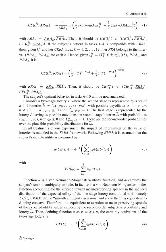
The subject’s optimal behavior in tasks 6–10 will be now analyzed.Consider a two-stage lottery L where the second stage is represented by a set of

n + 1 lotteries ˜lθ ∼ (x1, p1θ ; . . . ; xS, pSθ ), with possible payoffs x1 > · · · > xS ,θ ∈ {0, . . . , n}, psθ ≥ 0 and �S

s=1 psθ = 1. The first stage is represented by thelottery L having as possible outcomes the second-stage lotteries˜lθ with probabilities(q0, . . . , qn), with qθ ≥ 0 and �n

θ=0qθ = 1. These are the second-order probabilitiesover the plausible probability distributions for˜lθ .

In all treatments of our experiment, the impact of information on the value oflotteries is modeled in the KMM framework. Following KMM, it is assumed that thesubject’s ex ante utility is measured by:

u(CE(L)) = φ−1

(

n∑

θ=0

qθφ(EU(˜lθ ))

)

(3)

with

EU(˜lθ ) =S

∑

s=1

psθ u(xs).

Function u is a von Neumann-Morgenstern utility function, and φ captures thesubject’s smooth ambiguity attitude. In fact, φ is a von Neumann-Morgenstern indexfunction accounting for the attitude toward mean-preserving spreads in the induceddistribution of the expected utility of the one-stage lottery conditional to θ , namelyEU (˜lθ ). KMM define “smooth ambiguity aversion” and show that it is equivalent toφ being concave. Therefore, it is equivalent to aversion to mean-preserving spreadsof the expected utility values induced by the second-order subjective probability andlottery ˜lθ . Then, defining function v as v = φ ◦ u, the certainty equivalent of thetwo-stage lottery is

CE(L) = v−1

(

n∑

θ=0

qθ v(CE(˜lθ ))

)

, (4)

123


where CE(˜lθ ) is the certainty equivalent of the one-stage lottery conditional to θ .Function v is a von Neumann-Morgenstern index function accounting for the atti-tude toward mean-preserving spreads in certainty equivalents of the one-stage lotteryconditional to θ , namely CE(˜lθ ).

In each task of our experiment, there are only two possible payoffs, namely x, x ∈R+, x > x . Therefore, the small urn is represented by the 10-ball one-stage lottery˜lθ ∼ (x, pθ ; x, 1 − pθ ), where pθ = θ

10 is the objective probability given by theratio of the number of white balls θ ∈ {0, 1, . . . , 10} over 10. The second-orderprobabilities on the possible compositions of the small urn depend upon the treatmentunder consideration. In tasks 6–10 of treatments 1 and 2, the probability distribution(q0, . . . , q10) over the one-stage lotteries is objective. It is binomial in treatment 1 anduniform in treatment 2. Therefore, in treatment 1, given a task from 6 to 10, the second-order objective probabilities are always less dispersed than in the corresponding taskin treatment 2.13

Since in our experiment second-stage lotteries assigned to a subject in tasks 5–9have the same pair of outcomes, their variety only depends on first-order probabilities.Notice that the simple lottery in task 5, l j4

4 , is analogous to a two-stage lottery with all

second-stage lotteries ˜lθ=5 being l j44 , namely L5 := (q1, l j4

4 ; q2, l j44 ; ..; qn, l j4

4 ). It is

trivially assumed that L5 ∼ l j44 . In order to identify whether a subject shows aversion,

neutrality, or proneness to ambiguity, the subject’s answers to tasks 5 and 6 can becompared. In task 5, the subject is asked to value the unambiguous lottery that she hasselected in task 4. In task 6, the subject is asked to do the same for an ambiguous urnwith the same expected probability for the two outcomes. This suggests the followingoperational Definition 1.

Definition 1 (value-ambiguity attitude) Call C E(Lt ) the subject’s reservation pricefor the two-stage lottery assigned in task t ∈ {5, 6}. It can be interpreted as the certaintyequivalent of the two-stage lottery in task t . Then, a subject is value-ambiguity-averseif C E(L6) ≤ C E(L5). She is value-ambiguity-neutral if C E(L6) = C E(L5). She isvalue-ambiguity-loving if C E(L6) ≥ C E(L5).

In short, a value-ambiguity-averse subject values an ambiguous lottery less than itsunambiguous equivalent with the same mean probabilities. In the KMM model, thisis true if the subject’s φ function is concave.

Our experimental design offers an alternative to elicit ambiguity aversion by com-paring the subject’s answers to tasks 4 and 10. The two possible outcomes in lotteries{A, B, C, D} are the same in the two tasks. The difference lies in the fact that probabili-

13 In particular, in treatment 1, the objective second-order probabilities are as follows: in tasks 6 and10, q10 = q0 = 1/1024 � 0.1 %, q9 = q1 = 10/1024 � 1 %, q8 = q2 = 45/1024 � 4.4 %,q7 = q3 = 120/1024 � 11.7 %, q6 = q4 = 210/1024 � 20.5 %, and q5 = 252/1024 � 24.6 %;in task 7, q7 = q3 = 1/16 = 6.25 %, q6 = q4 = 4/16 = 25 %, and q5 = 6/16 = 37.5 %; intask 8, q10 = q3 = 1/128 � 0.8 %, q9 = q4 = 7/128 � 5.5 %, q8 = q5 = 21/128 � 16.4 %,q7 = q6 = 35/128 � 27.3 %; in task 9, q7 = q0 = 1/128 � 0.8 %, q6 = q1 = 7/128 � 5.5 %,q5 = q2 = 21/128 � 16.4 %, q4 = q3 = 35/128 � 27.3 %. All other qθ are zero. In treatment 2, theobjective second-order probabilities are: in tasks 6 and 10, qθ = 1/11 � 9.1 % for every θ = 0, 1, . . . , 10;in task 7, qθ = 1/5 for every θ = 3, 4, . . . , 7; in task 8, qθ = 1/8 for every θ = 3, 4, . . . , 10; in task 9,qθ = 1/8 for every θ = 0, 1, . . . , 7. All other qθ are zero.

123

G. Attanasi et al.

ties are unambiguously 1/2 in task 4, whereas they are ambiguous in task 10, with mean1/2. Defining a dispersion order on set {A, B, C, D}, such that D C B A,a more dispersed lottery is equivalent to a portfolio containing a larger share investedin the risky asset.

Definition 2 (choice-ambiguity attitude) Call jt ∈ {A, B, C, D} the index of thelottery chosen by a subject in task t ∈ {4, 10}. Then, a subject is choice-ambiguity-averse if j10 j4, i.e., if lottery j10 is not more dispersed than lottery j4. She ischoice-ambiguity-neutral if j10 = j4. She is choice-ambiguity-loving if j10 � j4, i.e.,lottery j10 is not less dispersed than j4.

Equivalently, a choice-ambiguity-averse subject will always reduce her demandfor the risky asset when the distribution of outcomes becomes ambiguous. In theKMM smooth ambiguity aversion framework, Gollier (2012) has shown that it isnot true in general that the concavity of the φ function implies the subject’s choice-ambiguity aversion. In other words, a smooth ambiguity-averse subject could have alarger demand for the ambiguous asset than another ambiguity-neutral subject withthe same risk aversion. However, Gollier (2012) provides a set of sufficient condi-tions on the structure of the two-stage uncertainty to re-establish the link between theconcavity of φ and ambiguity aversion. One of these sufficient conditions is that thedifferent second-stage distributions of the risky asset can be ordered by the MonotoneLikelihood Ratio stochastic order. Referring to the risky assets in Table 3, the set of

distributions of returns{

(yt , pθ ; yt, 1 − pθ ) |θ = 0, . . . , 10

}

in our ambiguous tasks

can always be ordered by the Monotone Likelihood Ratio. Thus, we conclude that,in the KMM framework, the two definitions of value-ambiguity aversion and choice-ambiguity aversion are equivalent in our experimental setting and are satisfied if φ isconcave. This justifies the following definition.

Definition 3 (coherent-ambiguity attitude) A subject is coherently-ambiguity-averseif CE(L6) ≤ CE(L5) and j10 j4, with at least one of the two relations holdingstrictly. She is coherently-ambiguity-neutral if CE(L6) = CE(L5) and j10 = j4. Sheis coherently-ambiguity-loving if CE(L6) ≥ CE(L5) and j10 � j4, with at least oneof the two inequalities holding strictly.

Our operational definition of coherent-ambiguity attitude is based on a double-check: the subject’s behavior is compared in task 5 versus task 6 and in task 4 versus task10. The first comparison shows whether, given the two second-stage lottery outcomes,the subject prefers to know first-order probability pθ than facing a mean-preservingspread of second-order probabilities over the all possible pθ . The second comparisonshows whether the subject prefers a less risky lottery (a less dispersed performance ofthe portfolio in Table 3) where this mean-preserving spread takes place.

The analysis will now turn to analyze how the certainty equivalent of the two-stage lottery varies when moving from task 6 to tasks 7, 8, or 9 and whether thisvariation depends on the fact that the subject is ambiguity-averse. First CE(L7) will becompared with CE(L6). It should be remembered that, in each of our three treatments,the two-stage lottery in task 7 is obtained from task 6 by symmetrically eliminatingthe plausibility of the extreme urns θ = 0, 1, 2, 8, 9, 10. This necessarily implies

123


qθ = 0 in task 7 for these θ . Compared to task 6, the subject’s subjective second-order probabilities must be symmetrically transferred from the extreme urns to theless dispersed urns θ = 3, . . . , 7. This yields a mean-preserving contraction in thedistribution of ˜U ∼ (EU(˜l0), q0; . . . ; EU(˜l10), q10), as will be shown. In the remainderof this section, u is normalized in such a way that u(x j4

4 ) = 0 and u(x j44 ) = 1, so that

EU (˜lθ ) = pθ .

Lemma 4 Consider a symmetric random variable p ∼ (p0, q0; . . . ; pn, qn), withpθ = θ/n, qθ = qn−θ for all θ , and n > 2. Consider another symmetric randomvariable p′ ∼ (p0, q ′

0; . . . ; pn, q ′n) on the same support, but with q ′

0 = q ′n = 0

and q ′θ = q ′

n−θ ≥ qθ = qn−θ for all θ ∈ {1, . . . , n − 1}. It implies that Eφ( p′) ≥Eφ( p) for all concave functions φ, i.e., that p′ is a Rothschild-Stiglitz mean-preservingcontraction of p.

Proof Observe that, by symmetry,

E p =n

∑

θ=0

qθ

θ

n=

n/2∑

θ=0

qθ

(

θ

n+ n − θ

n

)

=n/2∑

θ=0

qθ = 1

2.

Because the same observation can be made for p′, E p = E p′ = 1/2. Because p′ isobtained from p by a transfer of probability mass from the extreme states to the centerof the distribution, it is concluded that p is a mean-preserving spread of p′. �

Repeating this lemma three times, it turns out that C E(L7) must be larger thanC E(L6) under smooth ambiguity aversion. Because L7 is still ambiguous, C E(L7)

is smaller than C E(L5). Thus, C E(L5) ≥ C E(L7) ≥ C E(L6). The opposite resultwould hold under smooth ambiguity proneness. Observe that a crucial assumption forthe lemma is the symmetry of the second-order probability distributions. In treatments1 and 2, the second-order probability distribution on the composition of the small urn iseither binomial or uniform: both are clearly symmetric. In treatment 3, the symmetry ofthe second-order probability distribution will depend upon the subject’s beliefs on thecomposition of the big urn from which the small urn is built. However, the principle ofinsufficient reason suggests that the subject has symmetric beliefs on the compositionof the big urn, and, therefore, on the composition of the small urn generated by theBernoullian process. Under this principle, the following proposition can be written.

Proposition 5 If the subject is ambiguity-averse, then CE(L5) ≥ CE(L7) ≥ CE(L6).If she is ambiguity-loving, then CE(L5) ≤ CE(L7) ≤ CE(L6). If she is ambiguity-neutral, then CE(L5) = CE(L7) = CE(L6).

Tasks 8 and 9 will now be compared to task 6. Task 8 is similar to task 6 except thatthe worst urns have been eliminated. Proposition 6 shows that the certainty equivalentof the two-stage lottery assigned in task 8 is greater than the one of the two-stage lotteryassigned in task 6, whatever the degree of ambiguity of the subject, hence indepen-dently of the fact that she is ambiguity-averse, neutral, or loving. The opposite resultprevails for task 9, in which the best urns have been removed. Therefore, comparisonamong tasks 6, 8, and 9 always leads to C E(L8) ≥ C E(L6) ≥ C E(L9), whateverthe subject’s attitude toward ambiguity.

123

G. Attanasi et al.

Proposition 6 Suppose that new information implies that the worst (best) urns becomeimplausible, without reducing the probability qθ of any of the other urns. This newinformation raises (reduces) the certainty equivalent of the two-stage lottery indepen-dent of the degree of ambiguity aversion.

Proof Because φ is increasing and concave, it is obvious that any first-degreeor second-degree stochastic dominance improving shift in the distribution of(q0, EU(˜l0); . . . ; qn, EU(˜ln)) raises the certainty equivalent of the two-stage lottery.Because pθ = θ/n is increasing in θ, so is EU(˜lθ ) = pθu(x j4

4 ) + (1 − pθ )u(x j44 ).

Suppose that new information makes the worst lotteries (˜l0,˜l1, . . . ,˜lm), m < n,totally implausible. This implies that the new second-order probabilities take theform (q0, q1, . . . , qn), with q0 = q1 = · · · = qm = 0. This yields a first-degreestochastic improvement if qi ≥ qi for all i ∈ {m + 1, . . . , n} . Therefore, under theassumption that both u and φ are strictly monotone, this new information raises thecertainty equivalent of the lottery independent of the degree of ambiguity aversion. Ofcourse, the symmetric case also holds. Suppose that new information implies that thebest scenarios become implausible, without reducing the probability qθ of any of theother scenarios. This new information reduces the certainty equivalent of the lotteryindependent of the degree of ambiguity aversion. �

This result also applies to the comparison between task 8 (task 9) and task 7: thecertainty equivalent of the two-stage lottery assigned in the former task must be greater(smaller) than the one of the two-stage lottery assigned in task 6, whatever the degreeof ambiguity of the subject. Task 7 may be seen as a modification of task 9 through newinformation implying that the worst scenarios become implausible, without reducingthe probability qθ of any of the other scenarios in task 9. Task 7 may be also seenas a modification of Task 8 through new information implying that the best scenariosbecome implausible, without reducing the probability qθ of any of the other scenariosin task 8. Therefore, it follows that CE(L8) ≥ CE(L7) ≥ CE(L9) independent of theshape of φ.

An attempt will now be made to establish the complete ranking of the values oftasks 5–9 under smooth ambiguity aversion. Earlier, it has been noted that smoothambiguity aversion implies that CE(L5) ≥ CE(L7) ≥ CE(L6). Combining thesethree sequences of inequalities implies that, under smooth ambiguity aversion,

CE(L5)

CE(L8)

}

≥ CE(L7) ≥ CE(L6) ≥ CE(L9), (5)

independent of the subject’s attitude toward risk. The only degree of freedom undersmooth ambiguity aversion is thus given by the relative values of task 5 (no ambiguity:q5 = 1) and task 8 (ambiguity with worst urns eliminated: q0 = q1 = q2 = 0). Ifambiguity aversion is small enough, i.e., the concavity of φ is small, then the largeexpected probability of the high outcome enjoyed in task 8 will dominate the ambiguityaversion effect to yield C E(L8) > C E(L5), otherwise C E(L8) ≤ C E(L5). Thefollowing result is a direct consequence of Gollier (2001, Sect. 6.3.2).

123


Proposition 7 Suppose that a subject prefers the unambiguous lottery L5 to theambiguous lottery L8 (this is possible only under ambiguity aversion). Then, anincrease in ambiguity aversion in the KMM model can never reverse this ranking.

This implies that, assuming similar attitudes toward risk, any subject with CE(L5) <

CE(L8) has a smaller degree of smooth ambiguity aversion than any subject withCE(L5) ≥ CE(L8). Thus, comparing the values of task 5 and 8 for an ambiguity-averse subject will provide information about her degree of ambiguity aversion.

Of course, in the limit case of smooth ambiguity-neutrality,

CE(L8) > CE(L5) = CE(L6) = CE(L7) > CE(L9), (6)

independent of the subject’s attitude toward risk. Finally, for an ambiguity-lovingsubject,

CE(L8) ≥ CE(L6) ≥ CE(L7) ≥{

CE(L5)

CE(L9), (7)

independent of her attitude toward risk. If the degree of ambiguity proneness is smallenough, i.e., the convexity of φ is small, then the low expected probability of the highoutcome faced in task 9 will dominate the attractiveness of this ambiguous lottery forambiguity-loving subjects, so that CE(L9) < CE(L5), otherwise CE(L9) ≥ CE(L5).

Proposition 8 Suppose that a subject prefers the unambiguous lottery L5 to theambiguous lottery L9 (this is possible also under ambiguity proneness). Then, a con-cave transformation of theφ function in the KMM model can never reverse this ranking.

Thus, comparing the values of task 5 and 9 for an ambiguity-loving subject willprovide information about her degree of ambiguity proneness.

The next corollary shows the difference among certainty equivalents of two-stagelotteries in the same task of different treatments. The comparison of treatments 1 and 2is the easiest. The uniform distribution of the second-order probabilities in treatment 2is clearly a mean-preserving spread of the binomial distribution obtained in treatment1. Comparing the certainty equivalents for treatments 1 and 3 is more difficult. In bothtreatments, a Bernoullian process is applied to build the small urn, but the parameter ofthe Bernoulli distribution is p = 1/2 in treatment 1, whereas it is unknown in treatment3. If one accepts the principle of insufficient reason, then it may be assumed that thethird-order probabilities on parameter p yields Ep = 1/2. Under this assumption,treatment 3 always yields a mean-preserving spread of the second-order probabilitydistribution (q0, . . . , qn). Under ambiguity aversion, this yields a reduction of thecertainty equivalents. This yields the following result.

Corollary 9 If the subject is ambiguity-averse (-loving), then C Et is greater (smaller)in treatment 1 than in treatments 2 and 3 for every t = 6, 7, 8, 9.

By combining Proposition 7, Proposition 8, and Corollary 9, specific behavioralpredictions about possible treatment differences can be made. Although our experi-mental design is not within-subject, Tables 4 and 5 show that the distribution of thedegree of risk aversion does not differ among the three treatments, if both a CARA and a

123

G. Attanasi et al.

CRRA specification are used. Hence, if we assume that the distribution of the degree ofambiguity aversion is the same among the three treatments, then for similar degrees ofrisk aversion it should be found that the percentage of ambiguity-averse subjects withC E(L5) ≥ C E(L8) is lower in treatment 1 than in treatments 2 and 3. By combiningProposition 8 and Corollary 9 for ambiguity-loving subjects, a symmetrical predictionarises. Assume that the distribution of the degree of ambiguity proneness is the sameamong the three treatments. Then, the percentage of ambiguity-loving subjects withC E(L9) ≥ C E(L5) should be lower in treatment 1 than in treatments 2 and 3 withinthe same class of risk aversion.

4 Experimental results

In this section, our experimental results will be presented.14 First, in Sect. 4.1, theresults of the elicitation of the subjects’ risk attitude through the portfolio choicemethod implemented in (unambiguous) tasks 1–4 are analyzed. Then, in Sect. 4.2,subjects will be classified according to their ambiguity attitude relying on the oper-ational definition introduced in Sect. 3. In Sect. 4.3, the main theoretical predictionsderived in Sect. 3 will be tested. In Sect. 4.4, there will be an analysis of the treatmenteffects on the distribution of subjects’ beliefs over second-order probabilities and onthe certainty equivalents of two-stage lotteries in the ambiguous tasks.

4.1 Risk attitude elicitation

The portfolio choice method used at the beginning of the experiment enables allsubjects to face the same set of lotteries in tasks 1–4. This prompts a risk-attitudeordering of subjects independent of l j4

4 , the lottery chosen in task 4. This is the firstreason why such ordering is preferred to the certainty equivalent elicited in task 5,which instead depends on l j4

4 . Further, this specific portfolio choice method has theadvantage of imposing some theoretically derived constraints which allow to checkwhether the subject’s selected pattern is compatible with a CARA and/or a CRRAspecification. This provides an empirical verification of what is generally assumed inmany experimental studies on risk aversion.

First, a check is made on whether the portfolio choice method elicitation (tasks 1–4)leads to the same ordering in terms of CE(L5) as the (more standard) BDM mechanismproposed in task 5. Indeed, a positive (coeff. = 0.46) and highly significant (P value= 0.000) correlation is found between CE(L5) as predicted by the CARA orderingderived from the selected pattern in tasks 1–4 (see Table 4) and the one elicited throughthe BDM mechanism in task 5. If the CRRA is used in place of the CARA ordering (seeTable 5), the former correlation is slightly lower (coeff. = 0.36) and again statisticallysignificant (P value = 0.006).15

14 All raw data and statistical codes are available on request.15 More precisely, CE(L5) predicted by the CARA ordering is calculated as the average between

CE(lj44 ; AR Ah) and CE(l

j44 ; AR Ah) in (1), for h = 1, 2, . . . , 9. Similarly, CE(L5) predicted by the CRRA

ordering is calculated as the average between CE(lj44 ; RRAk ) and CE(l

j44 ; RRAk ) in (2), for k = 1, 2, . . . , 12.

123


Second, significant differences among the three treatments in the distribution ofCARA indexes or in the distribution of CRRA indexes are checked for. Although thepercentage of explained patterns under each specification is different in the Uniformtreatment (see respectively Tables 4, 5), no significant difference in the distribution ofrisk-aversion ordering in the three treatments is found. This is what Fig. 8 in the Appen-dix seems to suggest, if both a CARA and a CRRA specification are used. To providesupport to the graphical representation, two non-parametric tests have been conducted:a Kruskal–Wallis test16 and a Kolmogorov-Smirnov equality-of-distributions test witha pairwise comparison between treatments17. Both tests confirm no significant differ-ence in the distribution of both the CARA and the CRRA ordering among the threetreatments.18

Therefore, both orderings are correlated with the certainty equivalent of task 5and lead to similar distributions of risk attitude among treatments. Without assumingwhether subjects are CARA or CRRA, both specifications are used when analyzingpossible relations between the subject’s degree of risk aversion and her behavior intasks 6–10.

It is true that all the theoretical predictions derived in Sect. 3 within the KMMframework should hold whatever the subject’s risk aversion. Nevertheless possiblecorrelations between risk attitude and ambiguity attitude are checked for. A furthercheck is made about a possible role of risk attitude when testing our main theoreticalpredictions, which have been shown to hold independently of the subject’s risk attitude.Finally, including risk aversion as an explanatory variable in the econometric analysismay be useful in order to provide an experimental answer to some open theoreticalquestions such as the sign of CE(L8) − CE(L5) for ambiguity-averse subjects or thesign of CE(L9)−CE(L5) for ambiguity-loving ones. Notice that, for ambiguity-neutralsubjects, it is always CE(L8) > CE(L5) and CE(L9) < CE(L5).

4.2 Ambiguity attitude elicitation

In Table 6, subjects are classified as being ambiguity-averse, ambiguity-neutral, andambiguity-loving in each treatment according to Definition 3 (coherent-ambiguityattitude).19

16 The Kruskal–Wallis equality-of-populations rank test verifies the hypothesis that several samples arefrom the same population.17 The Kolmogorov-Smirnov test compares two observed distributions f (·) and g(·). The procedureinvolves forming the cumulative frequency distributions F(·) and G(·) and finding the size of the largest dif-ference between these. The hypothesis tested is whether the two observed distributions are equal (pairwisecomparisons between treatments 1–2, treatments 1–3, and treatments 2-3).18 According to the Kruskal–Wallis test the null hypothesis of equality of distributions (P value = 0.401for CARA and P value = 0.357 for CRRA) cannot be rejected. The Kolmogorov-Smirnov test confirms thisresult.19 EU maximizing subjects for the Binomial and Uniform treatments and subjective expected utility (hence-forth, SEU) maximizing subjects for the Unknown are both value-ambiguity-neutral and choice-ambiguity-neutral, hence coherent-ambiguity-neutral. However, given that the choice set in all our experimental tasksis discrete, it cannot be excluded that weekly non-EU (and non-SEU) maximizing subjects may fall into thegroup of coherent-ambiguity-neutral subjects. For example, consider a non-EU maximizing subject with

123

G. Attanasi et al.

Table 6 Classification of(coherent-)ambiguity attitudeaccording to Definition 3

Binomial Uniform Unknown Total

Coherent averse 13 15 17 45

Coherent neutral 16 5 8 29

Coherent loving 5 9 4 18

Total classified 34 29 29 92

Value averse & Choiceloving

1 4 2 7

Value loving & Choiceaverse

0 2 4 6

Total unclassified 1 6 6 13

Almost 1/2 of the classified subjects are ambiguity-averse, while less than 1/5 areambiguity-loving. Only 13 subjects (less than 12 % of the sample) participating in ourexperiment cannot be classified according to Definition 3: around half of them areambiguity-averse according to Definition 1 (value-ambiguity attitude) and ambiguity-loving according to Definition 2 (choice-ambiguity attitude). The other half of them arevalue-ambiguity-loving and choice-ambiguity-averse.20 Given the small percentageof unclassified subjects, it can be concluded that the concavity of the φ functionimplies choice-ambiguity aversion in our experimental tasks. This was exactly ourtheoretical prediction, given that the different second-stage distributions of the riskyasset have been set such that they can be ordered according to the Monotone LikelihoodRatio stochastic order (see Gollier 2012). Indeed, the correlation between strong value-ambiguity aversion (CE(L6) < CE(L5)) and strong choice-ambiguity aversion ( j10 ≺j4) is positive, not very high (coeff. = 0.18), but statistically significant (P value= 0.074). This last result will be further analyzed at the end of Sect. 4.3, by showingthat in our sample subjects with strong choice-ambiguity aversion are usually non-strongly value-ambiguity-averse.

From Table 6, one can also see that the percentage of classified subjects beingambiguity-averse is lower in the Binomial than in the Uniform treatment and in theUnknown treatment. Further, the percentage of classified subjects being ambiguity-neutral is higher in the Binomial than in the other two treatments.

Additional results can be stated by considering the “sign” of the ambiguity attitude.This is defined as being negative if the subject is ambiguity-averse, null if she isambiguity-neutral, and positive if she is ambiguity-loving. Looking at the multinomiallogistic regression of the sign of the ambiguity attitude over the treatment, it is foundthat the relative risk ratio for being ambiguity-neutral versus being ambiguity-averse is0.27 (P value = 0.040) when switching from the Binomial to the Uniform treatmentand 0.38 (P value = 0.091) when switching from the Binomial to the Unknown

Footnote 19 continueda strictly concave φ function, hence being ambiguity-averse. If the concavity of her φ function is small,then in our discrete choice set she could make the same choice as another subject with a linear φ function,hence ending up being classified as coherent-ambiguity-neutral.20 Although the number of unclassified subjects is lower in the Binomial than in the other two treatments,unclassified subjects are not statistically different from classified ones both with respect to CARA or CRRAordering and with respect to the lottery chosen in task 4.

123


treatment. In other words, the expected probability of being ambiguity-neutral seems tobe higher for subjects who participate in the Binomial treatment. Table 6 also shows thatthe percentage of subjects being ambiguity-loving is lower in the Binomial than in theUniform treatment, but not in the Unknown treatment. However, a multinomial logisticregression of the ambiguity attitude over the treatment shows that the relative risk ratiofor being ambiguity-loving versus being ambiguity-averse is 1.56 (not statisticallysignificant: P value = 0.510) when switching from the Binomial to the Uniformtreatment and 0.62 (not statistically significant: P value = 0.521) when switchingfrom the Binomial to the Unknown treatment.21

A possible explanation of this result relies on Corollary 9. Given the degree ofambiguity attitude, |CE(L6) − CE(L5)| is lower in the Binomial than in the Uniformtreatment. This is due to the fact that the distribution of second-order probabilities isless dispersed in the Binomial than in the Uniform treatment. Moreover, recall thatthe set of possible certainty equivalent values that a subject may select is discrete.Therefore, if a subject is slightly-ambiguity-averse or slightly-ambiguity-loving, it ismore likely for her to choose CE(L6) = CE(L5) in the Binomial than in the Uniformtreatment.22 The intuition based on Corollary 9 applies also to the comparison betweenthe Binomial and the Unknown treatment. Indeed, the percentage of ambiguity-averse(loving) subjects in the Unknown treatment is higher (lower) with respect to the othertwo treatments, although this difference is not significant (Kruskal–Wallis, P value= 0.258). However, by making a pairwise comparison between treatments about thepercentage of ambiguity-averse subjects, it is found that there is no statistically sig-nificant difference between the Binomial and the Uniform treatment (t test, P value= 0.290)23 and between the Uniform and the Unknown treatment (P value = 0.605),while the difference between the Binomial and the Unknown treatment is almost signif-icant (P value = 0.109). This distortion confirms our intuition about the interpretationof the Unknown treatment. In the Binomial and in the Unknown treatment, the 10-ball small urn in task 6 has been generated through the same Bernoullian process.However, the latter treatment is intrinsically more ambiguous, given that there is noinformation about the composition of the big urn from which the small unknown urnis generated. According to KMM, this generates smaller CE(L6) through (4) and/orlower j10 through (3) in the Unknown than in the Binomial treatment, thereby signif-icantly increasing the percentage of subjects for which it is CE(L6) ≤ CE(L5) andj10 j4. Notice that if value-ambiguity aversion and choice-ambiguity aversion aredisentangled, a higher percentage of ambiguity-averse subjects in the Unknown treat-ment is found than in the Binomial treatment, although this difference is not statisticallysignificant.

21 These results are not shown but can be made available upon request.22 This intuition is reinforced by the fact that the correlation between (strong) value-ambiguity-aversionand (strong) choice-ambiguity-aversion found above in all the sample of classified subjects is higher (coeff.= 0.45) and significant (P value = 0.007) only if the analysis is restricted at the Binomial treatment. Inthis treatment, it is plausible that only highly-ambiguity-averse subjects show at the same time CE(L6) <

CE(L5) and j10 ≺ j4.23 The t test is any statistical hypothesis test (parametric) in which the test statistic follows a Student’s tdistribution if the null hypothesis is supported. Here, a two-sample t test is run for a difference in mean (thenull hypothesis is that the two samples have the same mean).

123

G. Attanasi et al.

0.1

.2.3

.4.5

1 3 5 7 9 1 3 5 7 9 1 3 5 7 9

Averse Neutral LovingF

requ

ency

CARA index

0.1

.2.3

.4.5

1 3 6 9 12 1 3 6 9 12 1 3 6 9 12

Averse Neutral Loving

Fre

quen

cy

CRRA index

0.2

.4.6

.81

A B C D A B C D A B C D


Fre

quen

cy

Lottery chosen in task 4

a

b

Fig. 2 Risk-attitude orderings in tasks 1–4 and lottery chosen in task 4 by ambiguity attitude

This section will be concluded by analyzing the relation between the sign of theambiguity attitude and the degree of risk aversion. Figure 2a shows—through his-tograms and kernel density plots—that both the distribution of CARA indexes and the

123


distribution of CRRA indexes differ according to the sign of the ambiguity attitude.Indeed, under both specifications, the modal risk-aversion index for ambiguity-averseand for ambiguity-neutral is 1 (non-risk-averse subjects), while the modal index forambiguity-loving subjects is 8 (risk-averse subjects). Differences in the distributionsof our risk-aversion ordering among different signs of the ambiguity attitude are indeedfound to be significant.24 This supposed negative correlation between the sign of theambiguity attitude and the index of risk aversion is confirmed by rank correlation testsfor ambiguity-neutral subjects under CARA (coeff. = −0.28, P value = 0.063) and forambiguity-loving subjects under both specifications (under CARA: coeff. = −0.39,P value = 0.007; under CRRA, coeff. = −0.30, P value = 0.013). Such negativecorrelation is not found to be significant for ambiguity-averse subjects. However, ifambiguity-averse subjects are disentangled according to Definition 1 and Definition 2,the negative correlation between the fact of being choice-ambiguity-averse and theindex of risk aversion is found to be significant (under CARA: coeff. = −0.30, P value= 0.029; under CRRA: coeff. = −0.31, P value = 0.007). This last result is even morerelevant if one recalls that choice-ambiguity aversion was elicited (tasks 4 and 10) byrelying on the same method used to elicit risk aversion (tasks 1–4). Figure 2b seems toconfirm our intuition: very few ambiguity-averse subjects (less than 5 %) choose theleast risky lottery in task 4, while the vast majority of ambiguity-loving ones (61 %)choose this lottery in task 4; moreover, none of the latter chooses the riskiest lottery intask 4. Differences in the distribution of l j4

4 among the three groups of subjects averse,neutral, and prone to ambiguity are found to be significant.25

This point can be further clarified by bringing into the analysis the subject’s guesson the number of balls linked to the highest of the two lottery outcomes (henceforth,“winning balls”) in task 6, that could be interpreted as the subject’s modal belief on thecomposition of the small unknown urn. This guess may have influenced the certaintyequivalent in task 6 and so the sign of value-ambiguity aversion.26 Figure 9 in theAppendix reports the distribution of subjects’ guess on the number of winning ballsin tasks 6–9 disentangled by the sign of their ambiguity attitude (averse, neutral, andloving).27 By looking at the upper-left part of Fig. 9, one can notice that also the

24 In order to verify the equality in the distribution of each risk-aversion index among different signs ofthe ambiguity attitude, two different tests have been performed: Kruskal–Wallis equality-of-populationsrank test and Kolmogorov-Smirnov equality-of-distributions test. Both under CARA and under CRRA,the null hypothesis of equality in distributions can be rejected according to the Kruskal–Wallis equality-of-populations rank test (respectively for CARA and CRRA: P value = 0.010 , P value = 0.010). By performingthe Kolmogorov-Smirnov equality-of-distributions test with a pairwise comparison between different signsof the ambiguity attitude, the results are found to be consistent with the Kruskal–Wallis test.25 Again, a Kruskal–Wallis test has been performed to check whether the distribution of l

j44 is different

by treatment. According to this test, the null hypothesis of equality in distribution (P value = 0.000) canbe rejected. A Kolmogorov-Smirnov test has also been performed with a pairwise comparison betweendifferent signs of the ambiguity attitude, and the results are consistent with the Kruskal–Wallis test.26 The guess in task 6 is positively correlated (coeff. = 0.20, P value = 0.045) with the “normalized”CE(L6). In Sect. 4.4, the specific meaning of “normalized” certainty equivalent is explained.27 Recall that each unknown small urn in tasks 6–9 has 10 balls inside. Hence, the set of possible guessesin each of these tasks is {0, 1, . . . , 10}.

123

G. Attanasi et al.

distribution of subjects’ guess in task 6 is significantly different among different signsof the ambiguity attitude.28

Indeed, with a multivariate regression analysis it is found that—controlling or not fortreatment effect—both l j4

4 and the guess in task 6 are highly significant (respectively,P value = 0.000 and P value = 0.001): the former has a positive effect on beingambiguity-averse, while the latter has a negative one.

About the positive effect of l j44 , it may be thought that subjects have made some

kind of hedging between the higher risk they accepted through the choice of a riskylottery in task 4 and the ambiguous second-order probabilities over this (second-stage)lottery in task 10. Indeed, if value-ambiguity aversion and choice-ambiguity aversionare disentangled, a positive and highly significant correlation is found between l j4

4 andeach measure of ambiguity attitude: respectively, coeff. = 0.24 (P value = 0.023) forvalue-ambiguity aversion and coeff. = 0.42 (P value = 0.000) for choice-ambiguityaversion.

About the negative effect of the guess of the number of winning balls in task6, this plays a role through a decrease of CE(L6) and j10. Section 4.4 will showthat the distribution of subjects’ guess in task 6 does not depend on the treatmentwhere the subjects have participated, i.e., on the different distributions of second-order probabilities that have been generated through our experimental design.

4.3 Test of the main theoretical predictions

This section reports and comments on the percentage of classified subjects who satisfythe theoretical predictions stated in Sect. 3. Classified subjects are disentangled accord-ing to the sign of their ambiguity attitude (averse, neutral, and loving) and accordingto the treatment where they participated. All the theoretical predictions tested in thissection should hold independent of the treatment. A first set of theoretical predictions(Proposition 5) state different conditions for ambiguity-averse, ambiguity-neutral, andambiguity-loving subjects. A second set of theoretical predictions (Proposition 6)should hold whatever the sign of the ambiguity attitude.

Figure 3 summarizes the percentage of subjects classified according to Definition 3whose behavior in tasks 5–7 complies with Proposition 5. In particular, for 78 %(35/45) of ambiguity-averse subjects CE(L5) ≥ CE(L7) ≥ CE(L6); for 86 % (25/29)of ambiguity-neutral subjects CE(L5) = CE(L7) = CE(L6); for 78 % (14/18) ofambiguity-loving subjects CE(L5) ≤ CE(L7) ≤ CE(L6). Although the percentage ofsubjects fulfilling predictions of Proposition 5 is higher among the ambiguity-neutralones, the validity of said predictions does not depend on the sign of the ambiguityattitude. On the other hand, there is a weak dependence on the treatment. Througha t test, it is found that the percentage of subjects complying with Proposition 5 isalmost significantly higher in the Binomial (P value = 0.124) and in the Unknown

28 Through the Kruskal–Wallis test, we can reject the null hypothesis of equality in distribution (P value= 0.000). The Kolmogorov-Smirnov test confirms this result.

123


75%

67%

100%

25%

33%

0% 50% 100%

Loving

100%

60%

88%

40%

12%

0% 50% 100%

Neutral

82%

73%

77%

18%

27%

23%

0% 50% 100%

Averse

Unknown

Binomial

Proposition 5 does not hold

Uniform

Proposition 5 holds

Fig. 3 Percentage of subjects satisfying Proposition 5, by treatment and ambiguity attitude

(P value = 0.120) than in the Uniform treatment. Finally, this compliance is uncorre-lated with the subject’s CARA or CRRA ordering, as predicted by Proposition 5.29

Figure 4 reports the percentage of subjects whose behavior in tasks 6–9 complieswith Proposition 6 with regard to CE(L6) (Fig. 4a) and with regard to CE(L7) (Fig. 4b),respectively. Recall that Proposition 6 provides the same prediction for all subjectsbeing classified according to Definition 3, whatever the sign of their ambiguity attitudeand their degree of ambiguity aversion. It is easy to notice that the percentage ofsubjects fulfilling Proposition 6 is even higher than for Proposition 5 and that it doesnot depend on which of the two reference certainty equivalents have been applied,CE(L6) or CE(L7). In both cases, more than 90 % of ambiguity-averse subjects (42/45for CE(L6), 41/45 for CE(L7)), all ambiguity-neutral subjects (29/29), and more than70 % of ambiguity-loving subjects (13/18) comply with Proposition 6. As further proofof “rational” behavior of this huge percentage of subjects, it should be noted that thereare only 4/84 subjects satisfying Proposition 6 with regard to CE(L6) and not satisfyingit with regard to C E(L7); there are only 3/83 subjects who fulfill the predictions withregard to CE(L7) and not with regard to CE(L6).

There are no significant differences by treatment if CE(L6) is taken as reference. Ifinstead CE(L7) is taken as reference, the percentage of subjects being consistent withProposition 6 is slightly higher in the Binomial than in the Uniform treatment, withsuch difference being significant (P value = 0.055). On the other hand, whatever thereference certainty equivalent, CE(L6) or CE(L7), a significant difference is found bythe sign of the ambiguity attitude. Indeed, the percentage of ambiguity-loving subjectscomplying with Proposition 6 is significantly lower than the percentage of ambiguity-averse ones30 and the percentage of ambiguity-neutral ones31. Again, compliancewith the prediction of Proposition 6 is uncorrelated with the subject’s CARA or CRRAordering, in line with the theory.32

29 P value = 0.546 for CARA, P value = 0.841 for CRRA.30 P value = 0.023 for CE(L6), P value = 0.054 for CE(L7).31 P value = 0.002 for both CE(L6) and CE(L7).32 If CE(L6) is taken as reference, P value = 0.202 for CARA, P value = 0.278 for CRRA. If CE(L7) istaken as reference, P value = 0.216 for CARA, P value = 0.333 for CRRA.

123

G. Attanasi et al.

75%

67%

80%

25%

33%

20%

0% 50% 100%

Loving

100%

100%

100%

0% 50% 100%

Neutral

88%

100%

92%

12%

8%

0% 50% 100%

Averse

Unknown

Binomial


for CE(L6)

Uniform

Proposition 6 holds

for CE(L6)

100%

56%

80%

44%

20%

0% 50% 100%

Loving

100%

100%

100%

0% 50% 100%

Neutral

82%

93%

100%

18%

7%

0% 50% 100%

Averse

Unknown

Binomial


for CE(L7)

Uniform

Proposition 6 holds

for CE(L7)

a

b

Percentage of subjects satisfying CE(L8) ≥ CE(L6) ≥ CE(L9).

Percentage of subjects satisfying CE(L8) ≥ CE(L7) ≥ CE(L9).

Fig. 4 Percentage of subjects satisfying Proposition 6, by treatment and ambiguity attitude

Figure 5 shows the percentage of classified subjects whose behavior in tasks 5–9satisfies both Proposition 5 and Proposition 6 at the same time. As seen in Sect. 3, thetwo propositions taken together lead to relation (5) for ambiguity-averse, relation (6)for ambiguity-neutral, and relation (7) for ambiguity-loving subjects. Indeed, morethan 75 % of classified subjects (70/92) state their certainty equivalents in tasks 5–9 ina way that all the “rationality” constraints imposed by the KMM model are satisfied.It is interesting that between Proposition 5 and Proposition 6 the former cuts muchmore observations, given that percentages of verification in Fig. 5 are only slightlylower than those in Fig. 3. In addition, ambiguity-loving subjects have a lower ratio offulfillment of Propositions 5 and 6 taken together (61 %, 11/18) than ambiguity-aversesubjects (76 %, 34/45) and ambiguity-neutral ones (86 %, 25/29), although the formerdifference is not significant, possibly due to the low number of ambiguity-lovingsubjects in our sample. It should also be noted that all ambiguity-neutral subjectsfulfilling Proposition 5 also fulfill Proposition 6.

Furthermore, significant differences both by the sign of the ambiguity attitude andby treatment are encountered. About the former, we have anticipated above that thepercentage of ambiguity-loving subjects complying with both propositions is found

123


75%

44%

80%

25%

56%

20%

0% 50% 100%

Loving

100%

60%

88%

40%

12%

0% 50% 100%

Neutral

82%

67%

77%

18%

33%

23%

0% 50% 100%

Averse

Binomial

Relations (5), (6), (7) do not hold

Uniform

Relations (5), (6), (7) hold

Unknown

Fig. 5 Percentage of subjects satisfying (5), (6), and (7), by treatment and ambiguity attitude.[Note Relations (5), (6) and (7) refer respectively to ambiguity-averse, ambiguity-neutral and ambiguity-loving subjects]

Fig. 6 Disentanglement of low,medium, and high ambiguityaversion w.r.t.CE(L8) � CE(L5) andproneness w.r.t.CE(L5) � CE(L9)

to be significantly lower than the percentage of ambiguity-neutral ones (P value =0.038). About the latter, the percentage of subjects complying with both propositionsis significantly higher in the Binomial (P value = 0.038) and in the Unknown (P value= 0.018) than in the Uniform treatment. It is particularly striking that in the Unknowntreatment, all subjects satisfying Proposition 5 satisfy also Proposition 6, both withregard to CE(L6) and with regard to CE(L7). In fact, percentages of compliance withthe theoretical predictions are the same in Figs. 3 and in 5, whatever the sign ofthe ambiguity attitude. Once more, compliance with the entire set of our theoreticalpredictions is uncorrelated with the subject’s CARA or CRRA index.33

Finally, the subject’s behavior will be analyzed in the only two tasks for whichno sharp theoretical prediction is available. Reference here is made to tasks 5 and 8for ambiguity-averse subjects and to tasks 5 and 9 for ambiguity-loving ones. Fromrelation (6), in the limit case of smooth ambiguity-neutrality, CE(L8) > CE(L5) andCE(L5) > CE(L9) must hold. Therefore, in Fig. 6, ambiguity attitude is classified as“Low” for those ambiguity-averse subjects and for those ambiguity-loving ones whobehave like the ambiguity-neutral ones, respectively, in tasks 5 and 8 and in tasks 5and 9. “Medium” and “High” ambiguity attitudes are classified accordingly, that is a

33 P value = 0.838 for CARA, P value = 0.765 for CRRA.

123

G. Attanasi et al.

subject is highly-ambiguity-averse if CE(L8) < CE(L5) and highly-ambiguity-lovingif CE(L5) < CE(L9).

Surprisingly enough, the same percentage of highly-ambiguity-averse (10/45) andof highly-ambiguity-loving (4/18) subjects is found in our sample. Subjects in theformer group prefer to know the composition of the small urn with certainty (task 5)rather than knowing only that the worst scenarios are implausible (task 8). Specularly,subjects in the latter group prefer to know only that the best scenarios are implausible(task 9) rather than knowing the composition of the small urn with certainty (task 5).Notice that neither the sign of CE(L8) − CE(L5) for ambiguity-averse subjects northe sign of CE(L5) − CE(L9) for ambiguity-loving ones is correlated with any of theexplanatory variables introduced above (treatment, CARA ordering, CRRA ordering,lottery chosen in task 4, and guess on the winning balls, respectively, in task 8 and intask 9). The effects of all these variables are not significant at all, both in the univariateanalysis considering each control singularly and in the multivariate regressions. Theonly significant result detected is indeed counterintuitive. It is found that CE(L8) −CE(L5) > 0 depends positively on strong choice-ambiguity aversion (i.e., j10 ≺ j4).This would lead to conclude that strongly-choice-ambiguity-averse subjects are notso strongly-value-ambiguity-averse (CE(L6) < CE(L5)), thereby explaining why theabove found correlation between strong choice-ambiguity-attitude and strong value-ambiguity-attitude, although positive and significant, is not so high.

As anticipated at the end of Sect. 3, the combination of Proposition 7 and Corol-lary 9 suggests a possible treatment effect on the percentage of ambiguity-averse sub-jects showing CE(L5) ≥ CE(L8) and on the percentage of ambiguity-loving subjectsshowing CE(L9) ≥ CE(L5). Such prediction relies on the assumption of a similardistribution of risk attitude among the three treatments, which is satisfied, as shownin Sect. 4.1. Indeed, the prediction on the treatment effect over the size of the ambi-guity attitude is verified. The percentage of medium- and highly-ambiguity-aversesubjects is lower in the Binomial (31 %, 4/13) than in the Uniform (60 %, 9/15) andin the Unknown treatment (47 %, 8/17), with the difference being almost significantbetween the Binomial and the Uniform (P value = 0.131). Specularly, the percentageof medium- and highly-ambiguity-loving subjects is lower in the Binomial (40 %, 2/5)than in the Uniform (67 %, 6/9) and in the Unknown treatment (50 %, 2/4).

4.4 Treatment effects over beliefs and certainty equivalents

The analysis of the experimental results can be concluded by looking at possibletreatment effects over the certainty equivalent and over the guess of winning balls intasks 6–9.

Corollary 9 states that CE(Lt ) for t = 6, . . . , 9 should be higher in the Binomialthan in the Uniform and in the Unknown treatment. If the subject’s guess on winningballs in task t is correlated with CE(Lt ) for t = 6, . . . , 9, then it should be found thatthis guess should also be higher in the Binomial treatment. Now, it is true that ourexperimental design is between-subject; hence, it cannot be directly stated whetherand how a subject changes her certainty equivalent (and her guess) according to theway in which the unknown small urn is generated at the beginning of task 6. However,under the assumption that both the distribution of risk attitudes and the distribution

123


of ambiguity attitudes are not too different among treatments—that is what has beenshown, respectively, in Sect. 4.1 and in Sect. 4.2—possible treatment differences inthe distribution of certainty equivalents and of guesses in tasks 6–9 can be analyzed.

Figure 7 reports the distribution of subjects’ guess on the number of winning ballsin tasks 6–9 disentangled by treatment. The graphs by treatment seem to suggest thatthe distribution of guesses in the Unknown treatment is close to the one in the Binomialtreatment, and both are quite different from the one in the Uniform treatment. Thisresult is in line with the principle of insufficient reason, that should lead a subject inthe Binomial and in the Unknown treatment to provide a guess equal to 5 winningballs in tasks 6 and 7, between 6 and 7 winning balls in task 8, and between 3 and 4winning balls in task 9. Conversely, in the Uniform treatment, all guesses should beequivalent: any guess over a scenario that is plausible in a specific task is justifiable.

However, it is found that the distribution of a subject’s guess in task t is not signifi-cantly different among treatments, for t = 6, 8, 9.34 Our intuition is instead correct intask 7. According to the Kruskal–Wallis test on the equality in distribution of guesses bytreatment, the null hypothesis can be rejected at a 10 % level (P value = 0.082). Moreprecisely, according to the Kolmogorov-Smirnov equality-of-distributions test, thereis not equality in the distribution of guesses between the Binomial and the Uniformtreatment (P value = 0.003) and between the Unknown and the Uniform treatment (Pvalue = 0.016). Also in this specific task, it seems that the subjects in the Unknowntreatment state similar guesses to those of the subjects in the Binomial one.

Focusing on the relation between certainty equivalents and subjects’ guesses, over-all, the former are never found to be correlated with the latter in tasks 6–9 within thesame task.35

In general, certainty equivalents in task t (CE(Lt )) are negatively correlated withthe CARA and/or with the CRRA ordering (recall that the ordering index increases withrisk aversion). This is reasonable: as shown above, the subject’s certainty equivalentelicited in task 5 (and in the following four tasks) relies on the lottery chosen in task4. This choice also depends on the CARA or the CRRA ordering elicited in tasks 1–4(as seen in Sect. 4.2, this choice also influences the sign of the ambiguity attitude).

The link between certainty equivalent and risk aversion is further investigated byconsidering the lottery chosen in task 4 (l j4

4 ) and its relation with the “normalized”

values of the certainty equivalents, i.e., their index in tasks 6–9, with CE(Lt ) = x j44

being assigned index 1 and CE(Lt ) = x j44 being assigned index 11.36 Figure 10

in the Appendix shows the “normalized” values of CE(Lt ) for t = 6, . . . , 9. OnceCE(Lt ) are normalized, they are still found to be correlated with the risk-attitude index.

34 According to the Kruskal–Wallis test on the equality in distribution of guesses by treatment, the nullhypothesis cannot be rejected (respectively, for task 6, 8, 9, P value: 0.739, 0.375, 0.175). The Kolmogorov-Smirnov equality-of-distributions test with a pairwise comparison between treatments confirms this result.35 However, CE(L6) is positively correlated (coeff. = 0.35) with the guess in task 6 only in the Uniformtreatment (P value = 0.037). Also, CE(L9) is positively correlated (coeff. = 0.36) with the guess in task 9only in the Binomial treatment (P value = 0.035).36 In tasks 5–9, each subject always has the possibility to choose among eleven possible selling prices.

Therefore, for every t = 5, 6, . . . , 9 , index 1 can always be assigned to CE(Lt ) = xj44 , index 11 to

CE(Lt ) = xj44 and internal CE(Lt ) can be indexed accordingly. See footnote 5.

123

G. Attanasi et al.

0.2

.4.6

.8

1 3 5 7 9 1 3 5 7 9 1 3 5 7 9

Binomial Uniform UnknownFr

eque

ncy

Guess task 6

0.2

.4.6

.8

1 3 5 7 9 1 3 5 7 9 1 3 5 7 9

Binomial Uniform Unknown

Freq

uenc

y

Guess task 7

0.2

.4.6

.8

1 3 5 7 9 1 3 5 7 9 1 3 5 7 9


Freq

uenc

y

Guess task 8

0.2

.4.6

.8

1 3 5 7 9 1 3 5 7 9 1 3 5 7 9


Freq

uenc

y

Guess task 9

Fig. 7 Distribution of subjects’ guess on the number of “winning balls” in tasks 6–9 by treatment

However, while the relation between risk aversion and CE(L6), CE(L7) and CE(L8)

is negative, CE(L9) instead shows a positive relation with risk aversion. The lastresult can be referred to the positive correlation between risk aversion and ambiguityproneness highlighted in Sect. 4.2. Further, as long as the distribution of the second-order probabilities is symmetric around θ = 5 (tasks 6 and 7), the normalized certaintyequivalents are correlated with the guesses in the same task. Such correlation is notfound in tasks 8 and 9.

A strong regularity is that, by regressing either CE(Lt )or its normalized version overthe guess in the same task, the index of risk attitude and the treatment, no significanttreatment effects are found for any t = 6, 7, 8, 9.37 As one can notice from Fig. 10,the differences among treatments in the distribution of normalized CE(Lt ) are notstatistically significant for every t = 6, . . . , 9. In addition, the sign of all differencesCE(Lt+1) − CE(Lt ) for t = 5, 6, 7 and CE(Lt+2) − CE(Lt ) for t = 6, 7 do notdepend on the treatment.38

37 A relevant exception is again represented by the (normalized) certainty equivalent in task 7. Controllingfor CARA and treatment and taking the Binomial as reference treatment, the Unknown treatment has apositive and significant effect (P value = 0.059) over CE(L7). Controlling for CRRA and treatment, theUniform treatment also has a positive and significant effect (P value = 0.041) over CE(L7).38 To be more precise, only in the regressions for CE(L7) − CE(L6) > 0 (CE normalized), the Uniformtreatment significantly increases the probability that CE(L7) − CE(L6) > 0 with respect to the Binomialtreatment (P value = 0.040). This result also holds when controlling for the difference in the guesses aboutthe number of winning balls in task 7 and task 6.

123


All these findings lead to the following conclusion. Despite some differences in thedistribution of guesses among treatments, no treatment effect is found on the distrib-ution of certainty equivalents in the ambiguous tasks. Therefore, the only significantdifference among treatments is the one shown at the beginning of Sect. 4.2 about thedistribution of (CE(L6) − CE(L5)) if combined with the distribution of ( j10 − j4) ,i.e., the two conditions leading to state a subject’s coherent-ambiguity attitude.

5 A critical discussion vis-a-vis the experimental literature on ambiguityaversion

This section will attempt to frame this contribution into the experimental literatureon ambiguity aversion. An overview of previous contributions in the literature thatare relevant to this paper is presented in order to support our experimental design andto compare experimental results. To afford maximum clarity, this section has beendivided into four sub-sections, each treating different but complementary issues. Thefirst subsection will focus on the difference among risk, uncertainty, and ambiguity soas to clarify the definition given to each of these terms. Second, the issue of designingexperiments to discriminate between theories of ambiguity as well as to operationalizeone theory will be discussed. This study belongs to the latter category and evaluatesthe structure of (risk and) ambiguity attitudes within the KMM model. Third, theexperimental methods used to elicit risk and ambiguity will be looked at critically,taking into account previous experimental tests of these instruments. Finally, the fourthsub-section will compare our results with previous findings in the literature.

5.1 Risk, uncertainty, and ambiguity: distinguishing close concepts

The term “uncertainty” is often used as synonymous of both risk and ambiguityeven though these two terms identify different situations. The fundamental differencebetween risk and ambiguity concerns the distinction between whether probability isknown or unknown. This distinction can take different names: “measurable” uncer-tainty or risk, with known probabilities, and “unmeasurable” uncertainty or ambigu-ity, with unknown probabilities (Knight 1921); “precise” versus “vague” probability(Savage 1954); “unambiguous” versus “ambiguous” probability (Ellsberg 1961); andso forth. Espousing the general definition of risk, Harrison (2011) also provides adistinction between uncertainty and ambiguity based on the availability of relevantinformation to form subjective belief distribution: “When we have to worry about theunderlying nondegenerate distribution, when reduction of compound lotteries is notassumed, then we have moved from the realm of (subjective) risk to uncertainty. And,when the individual does not even have enough information to form any subjectivebelief distribution, degenerate or non-degenerate, we are in the realm of ambiguity” (p.352). However, in the literature, the term “ambiguity” is also often introduced whenthe individual forms a certain subjective belief distribution, but she faces “situationsin which some events do not have an obvious, unanimously agreeable, probabilityassignment” (Ghirardato 2004, p. 36).39

39 Ghirardato (2004) also discusses the issue of the formal definition of ambiguity and ambiguity attitude.

123

G. Attanasi et al.

Therefore, according to Harrison (2011), the KMM model pertains to the “mea-surable” uncertainty or risk realm. Consequently, all decision tasks of treatments 1–2and decision tasks 1–5 of treatment 3 deal with risk and uncertainty. Only decisiontasks 6–10 of treatment 3 refer to ambiguity. However, if the term “ambiguity” is alsoassociated to the case where the reduction of compound lottery axiom does not apply,then also decision tasks 6–10 of treatments 1–2 will also refer to ambiguity. This isthe meaning given to the term “ambiguity” within KMM and in this paper too.

5.2 Discriminating between theories versus operationalizing one theory

This sub-section reviews two broad classes of empirical contributions in decisionmaking under ambiguity. The first class includes previous empirical works aimedat designing experiments to discriminate between ambiguity models. These can bereferred to as “horse race” tests. The second class includes empirical contributionsaimed at operationalizing one model of ambiguity aversion. Within this latter class,only studies implementing a KMM-type experimental environment are reviewed here.

Within the first class, several papers have empirically investigated the descriptiveand predictive power of theories of decision making under ambiguity.40 Some of themhave studied ambiguity attitude by purposefully excluding two-stage probability mod-els.41 Complementary to these, some other papers (e.g., Conte and Hey 2013) investi-gated ambiguity attitude considering only two-stage probability models. Some othershave produced experimental designs aimed at comparing the performance of KMMwith that of non-expected utility models (Halevy 2007; Ahn et al. 2011). Halevy (2007)suggests that there is no unique theoretical model that universally captures ambiguitypreferences.42 In the same line, Conte and Hey (2013) compare the performance of dif-ferent theoretical decision models—expected utility, KMM, rank-dependent expectedutility, and Alpha model of Ghirardato et al. (2004)—through an experimental designslightly different from Halevy’s (2007). In fact, even though these two studies aresimilar for what concerns the implementation of ambiguity in the laboratory, theypresent some differences in the methodology.43 Conte and Hey’s (2013) results sug-gest that KMM performs best among the four tested models.44 However, not all exper-

40 Early literature is surveyed in Camerer and Weber (1992) and Camerer (1995).41 See for example Hey et al. (2010) and Hey and Pace (2014): both experimental designs are aimed attesting only non-two stage probability models.42 In particular, Halevy (2007) found that 15–20% of his subjects are ambiguity-neutral and able to reducecompound lotteries. Another 35 % of subjects exhibit ambiguity aversion (proneness) together with aversion(proneness) to mean-preserving spreads in the second-order distribution. Both these categories of subjectsare consistent with KMM.43 Indeed, both papers use Ellsberg-type urns. In particular, Conte and Hey (2013) adopted the sameurns 2 and 3 as Halevy (2007) that reproduce two-stage lotteries. However, Conte and Hey (2013) useexclusively pairwise questions to reduce the number of parameters to be estimated, no meaning to estimatea utility function. Differently, Halevy (2007) asks subjects to state certainty equivalents through the BDMmechanism so as to infer a utility function from the subject’s answers.44 The authors found results in favor of KMM both through individual estimates (56 % of subjects showbehavior consistent with KMM) and by classifying subjects according to posterior probabilities of each ofthem being coherent with one out of four types of preferences (50 % for KMM).

123


imental studies offer support for KMM. Ahn et al. (2011) found a result opposite toConte and Hey’s (2013) by performing a portfolio choice experiment45 aimed at inves-tigating rank-dependent theories versus smooth ambiguity. Their tests of significancesuggest that the majority of subjects are well described by the subjective expectedutility model. Moreover, among the remaining subjects, KMM fails to explain thebehavior of those showing ambiguity aversion.

Thus far, not many experiments have been designed with the explicit purpose of test-ing behavioral predictions within the KMM model only. Chakravarty and Roy (2009)is one of them. They have tried to separate attitude toward risk from that toward ambi-guity using the multiple price list method as the only experimental instrument. Theirmain objective consisted of investigating potential differences in subjects’ behaviorunder uncertainty over gains versus uncertainty over losses. They found a positive cor-relation between risk attitude and ambiguity attitude in the domain of gains (although,in the aggregate, subjects are risk-averse and ambiguity-neutral). Their result is notsole. Indeed, many empirical studies have found such positive correlation;46 only fewhave no correlation whatsoever.47 Within this class of studies, Andersen et al. (2009) isthe only experimental work that clearly states that the correlation between risk attitudeand ambiguity attitude can be negative. They estimated attitudes toward ambiguity,attitudes toward risk, and subjective probabilities in a rigorous manner within a KMM-type model, by making some parametric assumptions about the form of the distributionof the priors and the uncertain process. They found subjects who are risk-averse, andat the same time ambiguity-loving.

A new approach, which is becoming popular in experimental economics, is basedon adopting mixture models. These models have an important advantage with respectto subject-by-subject estimation through competing models. Heterogeneity acrossindividuals—a common finding of experimental studies on decision making underrisk and ambiguity—is captured within a unique model, which merges different the-ories explaining the behavior of different subjects in the same sample. Several papershave adopted this approach in decision making under risk. Cohen et al. (2011) considerEU and cumulative prospect theory (Tversky and Kahneman 1992); they also includea discussion of the previous use of mixture models in economics. Conte et al. (2011)consider EU and rank-dependent expected utility. More recently, this approach hasalso been adopted in decision making under ambiguity. Conte and Hey (2013), alongwith a subject-by-subject estimation of individuals’ preference functionals, estimateda mixture of EU, KMM, rank-dependent expected utility and Alpha model (Ghirardatoet al. 2004).

From a methodological point of view, these mixture models can be interpretedas a hybrid of the two classes of empirical contributions presented above, i.e., thosediscriminating between theories and those operationalizing one theory.

45 Ahn et al. (2011) implemented an experimental design where subjects are asked to choose betweendifferent lotteries that duplicate the return of a portfolio containing a safe asset and an ambiguous asset.46 Among several studies finding a positive correlation, see Lauriola and Levin (2001), Di Mauro andMaffioletti (2004), Bossaerts et al. (2010), and Ahn et al. (2011).47 Among the few detecting no correlation, see Cohen et al. (1987) and Cohen et al. (2011).

123

G. Attanasi et al.

Among those studies fitting none of the three categories above, a relevant one forcomparisons with this paper is Abdellaoui et al. (2011), which investigates the relation-ship between attitude toward risk, compound lotteries and ambiguity in a model-freesetting.

5.3 Strengths and weaknesses of our instruments

This subsection will critically evaluate the risk and ambiguity elicitation methodsused in this study. In particular, discussion will revolve around the flexibility of suchinstruments in coping with other questions not covered in this study.

It should be recalled that risk attitude was elicited through both a portfolio choicemethod (tasks 1–4) and a BDM mechanism (task 5).

It has been highlighted above that risk-attitude elicitation through portfolio choices(tasks 1–4) here carried out gives results similar to the more standard Holt and Laury(2002) method. If on the one hand this corroborates our first risk-elicitation instrument,on the other hand it raises doubt as to whether such instrument may suffer from thesame “order effects” problem of Holt and Laury (2002). In fact, moving from task1 to task 4, the subject’s “initial wealth” is non-decreasing (see Table 3). Further, intasks 3–4, the lotteries proposed always have an expected value higher than those intasks 1–2 (almost twice on average, as shown in Table 7 in the Appendix). Harrison etal. (2005) demonstrated and Holt and Laury (2005) confirmed the possibility of ordereffects by scaling up real payments by 10 or 20 times. In our design, this might notrepresent a problem, given that the scale from tasks 1–2 to tasks 3–4 is very low (1.8times on average). However, our design is easily adaptable to check for order effects.The order of presentation of tasks 1–4 may be inverted in some of the experimentalsessions, and possible differences in the distribution of the risk-aversion parameterbetween tasks 1–4 sessions and tasks 4–1 sessions may be investigated.

Our experimental design may be further refined to disentangle risk-neutral subjectsand risk-loving ones, which in Tables 4 and 5 are all assigned (respectively, CARAand CRRA) index 1. This will only require in tasks 1–4 some slight alterations in theset of possible lotteries in Table 2.48

The risk-attitude elicitation in task 5 also involves some reliability problems, pointedout in the literature by both experimental economists and theorists.

From an experimental point of view, Plott and Zeiler (2005) have expressed manyconcerns with the way that the BDM mechanism is popularly implemented. Ourinstructions and implementation of the BDM minimize these potential problems bytaking into account almost all of the features of Plott and Zeiler’s (2005) suggested

48 For example, the set of possible lotteries l jt (with j = A, B, C, D, and t = 1, 2, 3, 4) in Table 2 may be

enriched with just one lottery in task 4, namely l E4 = (40, 0.5; 0, 0.5). Then, under the CRRA specification,

subjects with RRA ∈ (−0.146, 0.123) would pick (lj11 , l

j22 , l

j33 , l

j44 ) = (D, D, D, D) and subjects with

RRA ∈ (−∞, −0.146) would pick (lj11 , l

j22 , l

j33 , l

j44 ) = (D, D, D, E). Notice that this would lead to

disentangle risk-neutral and risk-loving subjects as in Table 3 (p. 1649) of Holt and Laury (2002).

123


procedure.49 In this respect, to minimize the confusion effect,50 before task 5 of ourexperiment, subjects have received a thorough explanation of our BDM mechanismtogether with some numerical examples.51 Furthermore, as extensively underlined inSect. 2, a physical randomizing device is used to encourage each subject to see therandom buying price for her lottery (i.e., the one randomly selected by the “drawer”)as independent of her stated selling price. This also held for tasks 6–9, where theBDM was used for ambiguity-attitude elicitation. Finally, anonymity in decisions andin earnings was ensured. The similarities between our implementation of the BDMand the one in Plott and Zeiler (2005) may have prevented the endowment effect. Infact, Plott and Zeiler (2005) have found it to be insignificant, when sufficient controlshave been introduced in the BDM implementation.52

From a theoretical point of view, several researchers (e.g., Holt 1986) have pointedout that, when preferences do not satisfy the axioms underlying EU theory, the BDMmechanism may not elicit valuations accurately. In this regard, Karni and Safra (1987)have shown that the certainty equivalent of a lottery elicited using the BDM mechanismrespects the preference ordering if and only if preferences satisfy the independenceaxiom. This is assumed in our theoretical analysis, as we rely on KMM in choice underambiguity and as a consequence on EU in choice under risk.

About our ambiguity-elicitation instruments, an important issue raised in the lit-erature is subjects’ thinking about strategic behavior and/or manipulations by theexperimenter in Ellsberg-type tasks (Schneeweiss 1973; Kadane 1992). At the end ofSect. 2, we have presented all the features of the experimental design introduced toavoid such problems. First, all our instruments are physical instruments, and we neverrely on computer-generated realizations of random processes. Second, all subjectshave the chances to check any randomizing instrument before its implementation.Further, the randomization was handled in a manner so as to ensure that subjectsdid not assume that the experimenter was picking numbers and/or rearranging urnscomposition after “knowing” what the subjects choices were. For example, lotteries’random buying prices in the BDM in tasks 5–9 were drawn once for all these tasksbefore task 5 began. In treatment 1 and treatment 3, the composition of the unknownsmall urn used for tasks 6–10 was randomly determined before the beginning of task 6(see Fig. 1). Both the unknown small urns (treatment 1 and treatment 3) and the trans-parent construction urn (treatment 2) were left on a table in front of the experimental

49 See Harrison and Rutström (2008) for a deeper analysis of these and additional issues, as well asalternative elicitation methods. They also review useful techniques to estimate behavioral errors that couldarise in the calculation of reservation prices through the BDM mechanism.50 An important practical problem of each BDM mechanism is that it is complicated, and if subjects failto understand it, the elicited values might reflect their confusion and not their valuation.51 Differently from what recommended by Plott and Zeiler (2005), we did not introduce any practice roundbefore task 5. This is because we did not want subjects to have any feedback about random draws of buyingprices before going through the BDM mechanism in tasks 5–9. However, before task 5, both the drawerand each subject participating in the experiment were given the chance to check that each of the fourenvelopes—through which the BDM was physically implemented—contained the eleven numbered ticketshere indicated in footnote 5. Further, the fact that instructions of each new task were given prior to that taskallowed subjects to focus on a BDM at a time.52 To test for possible endowment effects, our experimental design should be extended to allow subjects toact as lottery sellers in some tasks (as in our experiment) and as lottery buyers in others.

123

G. Attanasi et al.

subjects from task 6 until the end of the experiment, i.e., until they were eventuallyused. In treatment 3, an additional random draw was made at the beginning of theexperiment to determine the color of the “winning balls” in the unknown small urn.53

Finally, all the previous operations were physically carried out by one of the subjectsshowing up for the experimental session, randomly chosen before its beginning andnot participating in the experiment. All these implementation devices were meant tomake our subjects aware that no manipulation from the experimenter was possibleabout the composition of the unknown small urn used for the ambiguous tasks.

Although the way we create “ambiguous” decision settings may seem less naturalthan alternative physical means in the experimental literature (e.g., the Bingo blowerused by Andersen et al. 2009, and by Hey et al. 2010), it is characterized by higherflexibility and lower distortions on the level of ambiguity a subject “objectively”perceives. For example, with a Bingo blower, one cannot physically produce our tasks6 and 10, characterized by the greatest possible level of ambiguity. In fact, during therotations of the Bingo blower, subjects cannot count the balls of each color, but theycan easily realize that there are balls of each color. Further, looking at its rotations,different subjects in the same session may have a different perception of the level ofambiguity, e.g., depending on the specific attention paid to the rotations and on thephysical distance of the subject from the Bingo cage.

One last comment should be made about our payment protocol. In our experiment,only one of the ten decision tasks was randomly selected at the end of the experimentto determine participants’ final earnings. Therefore, we use a random-lottery incen-tive mechanism (henceforth RLIM) with the twofold goal of obtaining no interactionbetween different decision tasks and proposing bigger stakes to our experimental sub-jects.54 In recent years, this payment protocol has become the most used incentivesystem for individual choice experiments, and many studies have used and tested itwith success.55 However, any payment protocol might in principle create distortionsin individual choice experiments, and even RLIM is not exempt from this potentialproblem, as recent studies have clearly shown.56 These recent findings have reported

53 See footnote 9.54 A possible theoretical criticism of the random-lottery incentive mechanism, put forward by Holt (1986),was demonstrated not to occur empirically by Starmer and Sugden (1991).55 Among the most recent, see Hey and Lee (2005) and Lee (2008).56 Cox et al. (2012) have compared the performance of several payment mechanisms in individual choicetasks and found a new mechanism—with the same expected value of payoff incentives as RLIM—thatis less biased than RLIM. With this new mechanism, at the end of the experiment, one state of nature israndomly drawn, and then all (comonotonic) lotteries chosen in the experiment are paid out for this stateof nature and the payoff divided by the number of tasks. Moreover, Harrison and Swarthout (2012) haveshown that preference estimates obtained under RLIM differ from those obtained in a one-task design and,more generally, documented concerns about the use of payment protocols over multiple choices that, asRLIM, assume the validity of the independence axiom. Similar concerns may be ascribed to the fact thatthe application of RLIM as payment protocol requires no violation of the reduction of compound lotteriesaxiom (henceforth ROCL). In this regard, Harrison et al. (2012) have found no violation of ROCL whensubjects are presented with only one choice and violation of ROCL when subjects are presented with manychoices and RLIM is used as a payment protocol.

123


distortions linked to the application of RLIM to experiments with several tasks underrisk. When unknown lotteries are introduced within one or more tasks (as in thispaper), distortions due to the use of RLIM as a payment protocol may be amplified.However, the opposite hypothesis may be equally reasonable in our study: due to thegreater “complexity” an ambiguous task involves, the subject may focus more on eachsingle task, as there is a compound lottery even within the task itself. This could leadthe subject to give less importance to the way a single task is selected for payment.Further research should explore and clarify this issue.

5.4 A comparison of our results with similar empirical studies

Within the two broad classes of empirical contributions in decision making underambiguity, this paper belongs to the second class: the KMM model is made opera-tional and the structure of risk and ambiguity attitudes is evaluated within this model.However, in this subsection, our study is compared with the closest previous contri-butions belonging to all groups indicated in Sect. 5.2. In particular, we focus here onthe differences in findings.

Within the first group of studies that have produced experimental designsaimed at comparing the performance of KMM to that of non-expected utilitymodels, Halevy (2007) is certainly the closest to our study in terms of experi-mental design. In fact, we use a similar BDM mechanism to elicit risk attitudeand value-ambiguity attitude. However, there are two main differences. On theone hand, compared to Halevy (2007), in our experimental design, the variationof the subject’s certainty equivalent is studied for a larger number of ambigu-ity levels and of distributions of second-order probabilities. Therefore, a richerset of theoretical relations—that a subject’s decisions should satisfy to be consis-tent with KMM—is formulated. On the other hand, three treatments—binomial,uniform, and unknown—are proposed between-subject. Halevy (2007) only pro-poses the last two treatments, and, more importantly, within-subject. With thisdesign, he can examine the relation between attitude toward ambiguity and atti-tude toward reduction of compound (objective) lotteries, a question which isoutside our scope of interest. Ahn et al. (2011) is also close to our experi-ment design. However, differently from their study, in each task of our experi-ment the asset contained in the portfolio is either safe or ambiguous. Moreover,we simplify the choice problem by limiting the choice set to only four possi-ble portfolios and considering an ambiguous environment with only two states ofnature.

The following is a discussion of our design against studies in the second group, i.e.,as our study, those explicitly designed to operationalize KMM. Here, experimentalresults will also be compared.

Similarly to Chakravarty and Roy (2009), our study separates attitude toward riskfrom that toward ambiguity. However, their main purpose radically differs from ours.They investigate potential differences in subjects’ behavior under uncertainty overgains versus uncertainty over losses, while in our experiment there are no negativeoutcomes. Moreover, we use portfolio choice questions and the BDM mechanism to

123

G. Attanasi et al.

elicit risk and ambiguity attitude, while they use the multiple price list method. Asanticipated above, they find a positive correlation between risk attitude and ambigu-ity attitude in the domain of gains, while our results tend to lean toward a negativecorrelation.

Our experimental findings about the performance of KMM are in line with Conteand Hey (2013): almost 9 out of 10 subjects in our experiment are classified as havinga coherent-ambiguity attitude within the KMM model, and almost 8 out of 10 ofthem satisfy all theoretical predictions derived within that model. Coherent-ambiguity-neutral subjects are those who have the highest percentage of compliance with KMMpredicted behavior. Recalling that for these subjects KMM reduces to the (subjective)expected utility model, we can relate this result to the one found by Halevy (2007)about the higher ability of ambiguity-neutral subjects to reduce compound lotteries.

Further, we find that highly-risk-averse subjects are more frequently ambiguity-loving than ambiguity-averse. This brings up the possible existence of a negativecorrelation between risk attitude and ambiguity attitude, as the one found by Andersenet al. (2009). It should be noticed that our experimental design only reveals the sign ofthe subject’s (coherent)-ambiguity attitude, i.e., whether she is (coherent)-ambiguity-averse, neutral, or loving. Sorting all classified subjects in three groups according to thissign, we find significant differences in the distributions of the degree of risk aversionamong the three groups. In particular, (coherent)-ambiguity-averse and (coherent)-ambiguity neutral subjects on average have a low degree of risk aversion, while thevast majority of (coherent)-ambiguity-loving subjects is highly-risk-averse. This pointrequires a more thorough discussion, provided in the next section.

Finally, we find that the percentage of coherently-ambiguity-averse subjects is lowerin the binomial than in the uniform and in the unknown treatment. However, only thedifference between the binomial and the unknown treatment is statistically significant.This result is partially in line with Abdellaoui et al. (2011), for the part where theystate that attitude toward ambiguity and attitude toward compound risks are related butdistinct, with this relationship being quite sensitive to the type of compound risks con-sidered. They define as compound risk those decision tasks where the second-orderprobability distribution over one-stage lotteries is objective: both our binomial andour uniform treatment belong to this category. In our study too, therefore, the rela-tion between what they call ‘ambiguity’ (our unknown treatment) and what they call‘compound risk’ depends on the type of compound risk considered, e.g., binomial oruniform. However, there are two crucial differences between our experimental designand the one implemented in Abdellaoui et al. (2011). First, although they analyze thesame uniform case as in our study, they do not treat the binomial case, focusing insteadon the hypergeometric case.57 Second and more importantly, as Halevy (2007), theyhave a within-subject design, while in our study a subject only participates in one treat-ment, hence facing only one of the second-order probability distributions (binomial,uniform, or unknown) that we generate so as to create ambiguity.

57 Their actual finding is that the hypergeometric case is the one having the strongest relationship withambiguity attitude.

123


6 Conclusion

This study indicates ways to identify two features of smooth ambiguity attitude à laKMM: value-ambiguity attitude and choice-ambiguity attitude. A value-ambiguity-averse subject values an ambiguous lottery less than its unambiguous equiva-lent with the same mean probabilities. A choice-ambiguity-averse subject alwaysreduces her demand for the risky asset when the distribution of outcomes becomesambiguous.

We elicit these two attitudes in a series of experimental decision tasks designedin order to match the main insights of the KMM model. Our decision tasks areparameterized so that a value-ambiguity-averse (-loving) subject should necessarilybehave as a choice-ambiguity-averse (-loving) one, i.e., showing coherent-ambiguityaversion. Indeed, we find that 88 % of our subjects (92/105) show a coherent-ambiguity attitude, independent of the treatment, i.e., the distribution of second-order probabilities (binomial, uniform, or unknown). This result clearly indicatesan equivalence between value-ambiguity aversion and choice-ambiguity aversionin subjects participating in our experiment. However, we do not find the sameequivalence between strong value-ambiguity aversion and strong choice-ambiguityaversion.

A key contribution of this paper is the theoretical analysis of ambiguous tasksdesigned to evaluate the structure of risk and ambiguity attitudes within the KMMmodel. In Sect. 3, we have provided two kinds of theoretical predictions: those hold-ing independent of the subject’s (coherent)-ambiguity attitude and those stating spe-cific behavior in correspondence of a specific attitude to (coherent)-ambiguity. Wefind that the former are satisfied by more than 90 % of our classified subjects (84/92),while the latter are complied with by more than 80 % of classified subjects (74/92).Overall, a large number of classified subjects (76 %, 70/92) satisfy all our theo-retically derived constraints. This remarkably high compliance of subjects’ behav-ior with KMM indirectly corroborates both our operational definition of (coherent)-ambiguity attitude and our experimental design being a correct representation of themain features of KMM in the laboratory. We do not find any significant correlationbetween compliance with KMM and gender, age, level of education, and degree of riskattitude.

A secondary contribution of this paper concerns the analysis of possible relationsbetween risk attitude and ambiguity attitude. We elicit risk attitude through the sametwo methods (portfolio choice and BDM) used to elicit the two features (respectively,choice and value) of coherent-ambiguity attitude. Risk-aversion orderings providedby the two methods are correlated. Relying on CARA or CRRA orderings of riskaversion built through the first method, we find that more than 1/2 of subjects maybe classified as CARA and almost 3/4 as CRRA. Under both specifications, we find anegative correlation between the degree of risk aversion elicited in the unambiguoustasks and the fact of showing coherent-ambiguity aversion in the ambiguous tasks.However, this correlation is significant if we consider only choice-ambiguity attitude.More specifically, in our sample many coherent-ambiguity-averse subjects have a lowdegree of risk aversion, while the most part of coherent-ambiguity-loving subjectshave a high degree of it (77 % of the coherent-ambiguity-loving subjects are in the last

123

G. Attanasi et al.

two quintiles of the CARA index distribution, and 73 % are in the last two quintiles ofthe CRRA index distribution).

A possible explanation for this apparently surprising result is as follows. This resultmay be linked to the riskiness of the second-stage lottery the subject chooses in theunambiguous task (that is the same she is assigned in the ambiguous task). The higherthe degree of risk aversion, the less risky the chosen lottery in the unambiguous task, thelower the subject’s value for this lottery, then, the lower the reduction of the subject’svalue for this lottery when the distribution of outcomes becomes ambiguous. Thepositive correlation between the riskiness of the lottery assigned in the most ambiguoustask and both value-ambiguity aversion and choice-ambiguity aversion that we find inthe data supports this explanation. However, this result is found in a between-subjectdesign: we ask a subject to state her certainty equivalent under different levels ofambiguity of the setting, but always facing the same pair of (second-stage) lotteryoutcomes. One may test whether the effect found between-subject also holds whenthe same subject is asked to state her attitude toward ambiguity for different pairs oflottery outcomes. This point is left for further research.

The third contribution of this paper concerns the analysis of subjects’ attitudes anddecisions in ambiguous tasks with specific distributions of second-order probabilities.We find that the percentage of coherently-ambiguity-averse subjects is lower (thoughnot significantly) in the binomial than in the uniform treatment. This was easily pre-dictable, as the latter distribution of second-order probabilities is a mean-preservingspread of the former. We also verify the prediction of a significantly lower percentageof coherent-ambiguity-averse subjects in the binomial than in the unknown treatment:indeed the latter is intrinsically more ambiguous than the former. A surprising fact isthe absence of a significant difference in the percentage of coherent-ambiguity-aversesubjects between the uniform and the unknown treatment. This may lead to validatethe assumption that subjective second-order probabilities may be thought as uniformlydistributed when the subject is not given any information about the composition of theunknown urn.

Acknowledgments The research leading to these results has received funding from the EuropeanResearch Council under the European Community’s Seventh Framework Programme (FP7/2007–2013)Grant Agreement No. 230589. G. Attanasi gratefully acknowledges financial support by the ChairGeorges Meyer in Mathematical Economics at Jean-Jacques Laffont Foundation (TSE). N. Pace grate-fully acknowledges financial support by the Swiss&Global and Fondazione Ca’ Foscari. The authors grate-fully thank Michèle Cohen, Sandrine Spaeter, Lorenzo Vantaggiato, participants at the 15th Conferenceon the Foundations and Applications of Utility, Risk and Decision Theory at Georgia State Universityin Atlanta, at the Workshop on New Developments in Decision Making under Uncertainty at Universitéde Cergy-Pontoise, and at a Cournot seminar at University of Strasbourg for their useful comments andsuggestions.

7 Appendix

7.1 Appendix A

For each lottery l jt = (x j

t , 0.5; x jt , 0.5) in Table 2, the expected value and the standard

deviation are respectively equal to EV = 0.5(x + x) and σ = 0.5(x − x). The two

123


Table 7 Risk attitude elicitation method: reinterpretation in terms of EV, σ, and (dσ/d EV )

Lottery Task t = 1 Task t = 2 Task t = 3 Task t = 4

EV j1 σ

j1

dσj

1

d EV j1

EV j2 σ

j2

dσj

2

d EV j2

EV j3 σ

j3

dσj

3

d EV j3

EV j4 σ

j4

dσj

4

d EV j4

j = A 9.0 3.0 3.0 8.5 2.5 5.0 17.0 3.0 3.0 16.5 2.5 5.0

j = B 10.0 6.0 3.0 9.0 5.0 5.0 18.0 6.0 3.0 17.0 5.0 5.0

j = C 11.0 9.0 3.0 9.5 7.5 5.0 19.0 9.0 3.0 18.0 10.0 5.0

j = D 12.0 12.0 3.0 10.0 10.0 5.0 20.0 12.0 3.0 19.0 15.0 5.0

lottery outcomes can be expressed in terms of the two moments, i.e., x = EV + σ

and x = EV − σ . In Table 7, the set of lotteries in tasks 1–4 are classified in terms ofthe triple

(

EV, σ, dσd EV

)

, where the ratio dσd EV is the same for all lotteries in the same

task. In particular, it is dσd EV = 3 in tasks 1 and 3, and dσ

d EV = 5 in tasks 2 and 4.

7.2 Appendix B

0.1

.2.3

.4.5

1 3 5 7 9 1 3 5 7 9 1 3 5 7 9


Fre

quen

cy

CARA index

0.1

.2.3

.4.5

1 3 6 9 12 1 3 6 9 12 1 3 6 9 12


Fre

quen

cy

CRRA index

Fig. 8 Distribution of CARA and CRRA index by treatment

123

G. Attanasi et al.

7.3 Appendix C

0.2

.4.6

.8

1 3 5 7 9 1 3 5 7 9 1 3 5 7 9


Fre

quen

cy

Guess task 6

0.2

.4.6

.8

1 3 5 7 9 1 3 5 7 9 1 3 5 7 9


Fre

quen

cy

Guess task 7

0.2

.4.6

.8

1 3 5 7 9 1 3 5 7 9 1 3 5 7 9


Fre

quen

cy

Guess task 8

0.2

.4.6

.8

1 3 5 7 9 1 3 5 7 9 1 3 5 7 9


Fre

quen

cy

Guess task 9

Fig. 9 Distribution of subjects’ guess on the number of “winning balls” in tasks 6–9 by ambiguity attitude

7.4 Appendix D

0.1

.2.3

.4

1 3 5 7 9 11 1 3 5 7 9 11 1 3 5 7 9 11


Fre

quen

cy

Task 6

0.1

.2.3

.4

1 3 5 7 9 11 1 3 5 7 9 11 1 3 5 7 9 11


Fre

quen

cy

Task 7

0.1

.2.3

.4

1 3 5 7 9 11 1 3 5 7 9 11 1 3 5 7 9 11


Fre

quen

cy

Task 8

0.1

.2.3

.4

1 3 5 7 9 11 1 3 5 7 9 11 1 3 5 7 9 11


Fre

quen

cy

Task 9

Fig. 10 Distribution of “normalized” CE(Lt ) in tasks 6–9 by treatment

123


References

Abdellaoui, M., Klibanoff, P., & Placido, L. (2011). Ambiguity and compound risk attitudes: An experiment.Working paper. Northwestern University.

Ahn, D., Choi, S., Gale, D., & Kariv, S. (2011). Estimating ambiguity aversion in a portfolio choiceexperiment. Working paper. University of California, Berkeley.

Andersen, S., Fountain, J., Harrison, G., & Rutström, E. (2009). Estimating aversion to uncertainty. Workingpaper. University of Central Florida.

Arrow, K. (1964). The role of securities in the optimal allocation of risk bearing. Review of EconomicStudies, 31, 91–96.

Attanasi, G., & Montesano, A. (2012). The price for information about probabilities and its relation withrisk and ambiguity. Theory and Decision, 73, 125–160.

Becker, G., DeGroot, M. H., & Marschak, J. (1964). Measuring utility by a single response sequentialmethod. Behavioral Science, 9, 226–232.

Becker, S. W., & Brownson, F. O. (1964). What price ambiguity? Or the role of ambiguity in decisionmaking. Journal of Political Economy, 72, 62–73.

Bossaerts, P., Ghirardato, P., Guarnaschelli, S., & Zame, W. (2010). Prices and allocations in asset marketswith heterogeneous attitudes towards ambiguity. Review of Financial Studies, 23, 1325–1359.

Camerer, C. (1995). Individual decision making. In J. Kagel & A. Roth (Eds.), Handbook of experimentaleconomics (pp. 587–703). Princeton University Press.

Camerer, C., & Weber, M. (1992). Recent development in modeling preferences: Uncertainty and ambiguity.Journal of Risk and Uncertainty, 5, 325–370.

Chakravarty, S., & Roy, J. (2009). Recursive expected utility and the separation of attitudes towards riskand ambiguity: An experimental study. Theory and Decision, 66, 199–228.

Cohen, M., Jaffray, J.-Y., & Said, T. (1987). Experimental comparison of individual behavior under risk andunder uncertainty for gains and for losses. Organizational Behavior and Human Decision Processes, 39,1–22.

Cohen, M., Tallon, J. M., & Vergnaud, J. C. (2011). An experimental investigation of imprecision attitudeand its relation with risk attitude and impatience. Theory and Decision, 71, 81–109.

Conte, A., Hey, J. D. (2013). Assessing multiple prior models of behavior under ambiguity. Journal of Riskand Uncertainty, 46, 113–132.

Conte, A., Hey, J. D., & Moffatt, P. G. (2011). Mixture models of choice under risk. Journal of Econometrics,162, 79–82.

Cox J. C., Sadiraj V., & Schmidt U. (2012). Paradoxes and mechanisms for choice under risk. ExperimentalEconomics Center Working Paper Series 2012-08, Experimental Economics Center, Andrew YoungSchool of Policy Studies, Georgia State University.

Di Mauro, C., & Maffioletti, A. (2004). Attitudes to risk and attitudes to uncertainty: Experimental evidence.Applied Economics, 36, 357–372.

Ellsberg, D. (1961). Risk, ambiguity and the Savage axioms. Quarterly Journal of Economics, 75, 643–669.Epstein, L. G. (2010). A paradox for the “smooth ambiguity” model of preference. Econometrica, 78,

2085–2099.Fischbacher, U. (2007). z-Tree: Zurich toolbox for ready-made economic experiments. Experimental Eco-

nomics, 10, 171–178.Ghirardato, P. (2004). Defining ambiguity and ambiguity attitude. In I. Gilboa (Ed.), Uncertainty in economic

theory: A collection of essays in honor of David Schmeidler’s 65th birthday (pp. 36–45). London:Routledge.

Ghirardato, P., Maccheroni, F., & Marinacci, M. (2004). Differentiating ambiguity and ambiguity attitude.Journal of Economic Theory, 118, 133–173.

Gollier, C. (2001). Should we beware of the precautionary principle? Economic Policy, 16, 301–328.Gollier C. (2012). Optimal insurance design of ambiguous risks. IDEI Working Paper no. 718.Halevy, Y. (2007). Ellsberg revisited: An experimental study. Econometrica, 75, 503–536.Harrison, G. W. (2011). Experimental methods and the welfare evaluation of policy lotteries. European

Review of Agricultural Economics, 38, 335–360.Harrison, G. W., Johnson, E., McInnes, M. M., & Rutström, E. E. (2005). Risk aversion and incentive

effects: Comment. American Economic Review, 95, 897–901.

123

G. Attanasi et al.

Harrison, G. W., Martinez-Correa, J., & Swarthout J. T. (2012). Reduction of compound lotteries withobjective probabilities: Theory and evidence. Working Paper 2012–05, Center for the Economic Analysisof Risk, Robinson College of Business, Georgia State University.

Harrison, G. W., & Rutström, E. E. (2008). Risk aversion in the laboratory. In G. W. Harrison & J. Cox(Eds.), Risk aversion in experiments (pp. 41–196). Bradford, UK: JAI Press.

Harrison, G. W., & Rutström, E. (2009). Expected utility theory and prospect theory: One wedding and adecent funeral. Experimental Economics, 12, 133–158.

Harrison G. W., & Swarthout T. (2012). The independence axiom and the bipolar behaviorist. ExperimentalEconomics Center Working Paper Series 2012–01, Experimental Economics Center, Andrew YoungSchool of Policy Studies, Georgia State University.

Hey, J. D., & Lee, J. (2005). Do subjects separate (or are they sophisticated)? Experimental Economics, 8,233–265.

Hey, J. D., Lotito, G., & Maffioletti, A. (2010). The descriptive and predictive adequacy of theories ofdecision making under uncertainty/ambiguity. Journal of Risk and Uncertainty, 41, 81–111.

Hey, J. D., & Pace, N. (2014). The explanatory and predictive power of non two-stage-probability theoriesof decision making under ambiguity. Journal of Risk and Uncertainty (forthcoming).

Holt, C. A. (1986). Preference reversal and the independence axiom. American Economic Review, 76,508–515.

Holt, C. A., & Laury, S. K. (2002). Risk aversion and incentive effects. American Economic Review, 92,1644–1655.

Holt, C. A., & Laury, S. K. (2005). Risk aversion and incentive effects: New data without order effects.American Economic Review, 95, 902–912.

Kadane J. B. (1992). Healthy skepticism as an expected-utility explanation of the phenomena of Allais andEllsberg. In: Geweke J. (Ed.), Decision making under risk and uncertainty: New models and empiricalfindings. Boston: Kluwer. (And in Theory and Decision, 32, 57–64).

Karni, E., & Safra, Z. (1987). ‘Preference reversal’ and the observability of preferences by experimentalmethods. Econometrica, 55, 675–685.

Klibanoff, P., Marinacci, M., & Mukerji, S. (2005). A smooth model of decision making under ambiguity.Econometrica, 73, 1849–1892.

Klibanoff, P., Marinacci, M., & Mukerji, S. (2012). On the smooth ambiguity model: A reply. Econometrica,80, 1303–1321.

Knight, F. (1921). Risk, uncertainty, and profit. Boston: Houghton Mifflin.Lauriola, M., & Levin, I. P. (2001). Relating individual differences in attitude toward ambiguity and risky

choices. Journal of Behavioral Decision Making, 14, 107–122.Lee, J. (2008). The effect of the background risk in a simple chance improving decision model. The Journal

of Risk and Uncertainty, 36, 19–41.Machina, M. (2004). Almost objective uncertainty. Economic Theory, 24, 1–54.Plott, C. R., & Zeiler, K. (2005). The willingness to pay-willingness to accept gap, the “endowment

effect”, subject misconceptions, and experimental procedures for eliciting valuations. American Eco-nomic Review, 95, 530–545.

Pratt, J. W. (1964). Risk aversion in the small in the large. Econometrica, 32, 122–136.Quiggin, J. (2007). Ambiguity and the value of information: An almost-objective events analysis. Economic

Theory, 30, 409–414.Savage, L. J. (1954). The foundations of statistics. New York: Wiley.Schneeweiss, H. (1973). The Ellsberg Paradox from the point of view of game theory. Inference and

Decision, 1, 65–78.Snow, A. (2010). Ambiguity and the value of information. Journal of Risk and Uncertainty, 40, 133–145.Starmer, C., & Sugden, R. (1991). Does the random-lottery incentive system elicit true preferences? An

experimental investigation. American Economic Review, 81, 971–978.Tversky, A., & Kahneman, D. (1992). Advances in prospect theory: Cumulative pepresentation of uncer-

tainty. Journal of Risk and Uncertainty, 5, 297–323.

123

Eliciting ambiguity aversion in unknown and in compound lotteries: a smooth ambiguity model...

Documents

Transcript of Eliciting ambiguity aversion in unknown and in compound lotteries: a smooth ambiguity model...