Survey Review

Search procedure for improving Modified Ambiguity Function Approach--Manuscript Draft--

Manuscript Number: SRE102

Full Title: Search procedure for improving Modified Ambiguity Function Approach

Article Type: Research Paper

Section/Category: Refereed paper

Keywords: GNSS data processing, Ambiguity Function, MAFA method

Corresponding Author: Slawomir Cellmer

POLAND

Corresponding Author SecondaryInformation:

Corresponding Author's Institution:

Corresponding Author's SecondaryInstitution:

First Author: Slawomir Cellmer

First Author Secondary Information:

Order of Authors: Slawomir Cellmer

Order of Authors Secondary Information:

Abstract: The Modified Ambiguity Function Approach (MAFA) is a method of GNSS carrierphase data processing. In this method, the functional model of the adjustment problemcontains the conditions ensuring the "integerness" of the ambiguities. These conditionsare expressed in the form of differentiable function. A prerequisite for obtaining thecorrect solution is a mechanism ensuring not only the "integerness" of the ambiguitiesbut also appropriate convergence of the computational process. One of suchmechanisms is a cascade adjustment, applying the linear combinations of the L1 andL2 signals with the integer coefficients and various wavelengths. Another method ofincreasing the efficiency of the MAFA method is based on the application of the integerdecorrelation matrix to transform observation equations into equivalent, but betterconditioned, observation equations. This paper presents the search procedure as thenext technique of improving the MAFA method. This technique together with thedecorrelation procedure allows to reduce the number of stages of the cascadeadjustment and to obtain correct solution even in the case when a priori position is afew meters away from the actual position. In this paper an example of data processingusing the proposed algorithm is given. The results of numerical tests based on realdata are presented.

Powered by Editorial Manager® and Preprint Manager® from Aries Systems Corporation

Search procedure for improving Modified Ambiguity Function Approach

Slawomir Cellmer

University of Warmia and Mazury in Olsztyn, Poland

email: slawomir.cellmer@gmail.com

ABSTRACT

The Modified Ambiguity Function Approach (MAFA) is a method of GNSS carrier phase data

processing. In this method, the functional model of the adjustment problem contains the conditions

ensuring the "integerness" of the ambiguities. These conditions are expressed in the form of

differentiable function. A prerequisite for obtaining the correct solution is a mechanism ensuring not

only the "integerness" of the ambiguities but also appropriate convergence of the computational

process. One of such mechanisms is a cascade adjustment, applying the linear combinations of the L1

and L2 signals with the integer coefficients and various wavelengths. Another method of increasing

the efficiency of the MAFA method is based on the application of the integer decorrelation matrix to

transform observation equations into equivalent, but better conditioned, observation equations. This

paper presents the search procedure as the next technique of improving the MAFA method. This

technique together with the decorrelation procedure allows to reduce the number of stages of the

cascade adjustment and to obtain correct solution even in the case when a priori position is a few

meters away from the actual position. In this paper an example of data processing using the proposed

algorithm is given. The results of numerical tests based on real data are presented.

KEY WORDS: GNSS data processing, Ambiguity Function, MAFA method.

INTRODUCTION

The MAFA method is based on the least squares adjustment (LSA) with condition

equations in the functional model of the adjustment problem [2],[3],[4],[5]. This

ensures that the condition of the ambiguity „integerness‖ is satisfied in the final

results. The functional model for the carrier phase adjustment is relatively weak.

Therefore different linear combinations (LC) of L1 and L2 GPS carrier phase

observations are applied in the cascade adjustment so that the appropriate

convergence of the computational process can be assured [9],[12]. Another method

of improving the efficiency of the MAFA method was proposed by Cellmer [3],[4].

This technique exploits an integer decorrelation procedure. After transformation of

the observation equations with an integer decorrelation matrix, a model of an

adjustment problem turns into an equivalent model, but a better conditioned one.

There are some limitations in applying the MAFA method. Cellmer [3] derived the

necessary condition for obtaining correct solution with MAFA method. This

condition is associated with the accuracy of the a priori position and the wavelength

of LC forming an observation set. The a priori position must be placed inside a

certain region around the actual position. Therefore the approximate position in

carrier phase process should be as good as possible. The accuracy of the approximate

position can be increased using Network Code DGPS Positioning [1]. However this

accuracy can be still insufficient for MAFA method, even if the decorrelation

procedure and the cascade adjustment are applied. Therefore, in this paper, the search

procedure is proposed, as the technique of overcoming this problem. This procedure

is based on testing the objective function values for different vectors of misclosures

in the functional model of the adjustment problem. The misclosures vector is

described in details in section 3. This procedure allows obtaining correct solution,

even if the a priori position is a few meters away from the actual position. The next

ManuscriptClick here to download Manuscript: cellmer_paper1.docx

1 2 3 4 5 6 7 8 9 10 11 12 13 14 15 16 17 18 19 20 21 22 23 24 25 26 27 28 29 30 31 32 33 34 35 36 37 38 39 40 41 42 43 44 45 46 47 48 49 50 51 52 53 54 55 56 57 58 59 60 61 62 63 64 65

section presents the theoretical basis of the MAFA method followed by the

description of the techniques improving its efficiency. In the third section the search

procedure is presented. In the last part of the paper a numerical example, the results

of the tests and some conclusions are given.

MAFA METHOD

The following simplified form of the observation equation for double differenced

(DD) carrier phase observable is assumed, [11],[13],[16]:

, (1)

where:

– DD carrier phase observable (in cycles)

– signal wavelength

v – residual (measurement noise)

Xc – receiver coordinate vector

(Xc) – DD geometrical range

N – integer number of cycles (DD initial ambiguity)

Then taking into account the integer nature of the ambiguity parameter N and

assuming that the residual values are much lower than half a cycle, [2],[11], the Eq.

(1) can be rewritten in the following form:

(2)

or

, (3)

where round is a function of rounding to the nearest integer value. The residual (3)

takes into account the integer nature of ambiguities. The right side of the Eq. (3) can

be expressed in the form of the following, differentiable and continuous function,

[4],[5]:

, (4)

where s is an auxiliary variable:

. (5)

Each of the DD carrier phase observations is linearized. After linearization, the

general formula of the residual equations can be shown in the following form:

V= AX+, (6)

with:

(7)

1cλ

Φ+v= ρ X N

1 1λ λ

Φ+v- ρ=round Φ- ρ

1 1λ λ

v=round Φ- ρ Φ- ρ

1arcsin[sin( s)]for s s : cos( s) 0

round(s) s1

arcsin[sin( s)]for s s : cos( s) 0

1s

1 1 1

2 2 2

n n n

x y z

x y z

x y z

A

1 2 3 4 5 6 7 8 9 10 11 12 13 14 15 16 17 18 19 20 21 22 23 24 25 26 27 28 29 30 31 32 33 34 35 36 37 38 39 40 41 42 43 44 45 46 47 48 49 50 51 52 53 54 55 56 57 58 59 60 61 62 63 64 65

(8)

where:

V – residual vector (n×1),

X – parameter vector (increments to a priori coordinates vector X0),

A – design matrix (n×3),

∆ – misclosures vector (n ×1),

0 – DD geometric distance vector computed using a priori position and

satellite coordinates.

The LS solution of the formula (6) is:

X = -(ATPA)

-1A

TP, (9)

with P standing for the weight matrix.

In order to assure the convergence of the computational process to the correct

solution, in classic form of MAFA method, three linear combinations (LC) of L1 and

L2 GPS carrier phase observables with integer ambiguities and longer wavelengths

are applied in the cascade adjustment [2]. The computations are performed

successively for three LC, starting from -3L1+4L2 followed by L1-L2 and finishing

with L1 signal only. The efficiency of the MAFA method can be also improved using

the decorrelation procedure. The ambiguities (N) are usually strongly correlated.

Hence, fixing one value of ambiguity through rounding value s in (5) to the nearest

integer as in (2), has an impact on the rest of the ambiguities. Therefore, the

correlation between ambiguities should be taken into account at rounding the right

side of the Eq. (2) or alternatively the observation equations should be transformed

into the equivalent form with decorrelated ambiguities.

Let us assume that Z is the integer decorrelation matrix [14], [15]:

QNz = ZQNZT, (10)

where:

QN – ambiguity covariance matrix

QNz – diagonal transformed ambiguity covariance matrix.

By multiplying Eq. 1 with Z, one can obtain a new equation with a new integer

ambiguity vector Nz:

. (11)

The above formula can replace Eq. (1). Further considerations are the same but

decorrelated observation Eq. (11) in the place of Eq. (1) increases the probability of

obtaining the correct solution. The subsequent part of the computation process results

from this equation. There are many various methods of finding the Z decorrelation

matrix [10],[14],[18]. In order to find the Z matrix, the ambiguity covariance matrix

(QN) is required. This matrix can be evaluated on the basis of the system of

observation equations (1) after linearization:

V=AX+BN–L, (12)

where:

L – misclosures (observed minus computed) vector

B – ambiguity functional model matrix

1 1

0 0round

1Z CZ ZZ

V (X ) N

1 2 3 4 5 6 7 8 9 10 11 12 13 14 15 16 17 18 19 20 21 22 23 24 25 26 27 28 29 30 31 32 33 34 35 36 37 38 39 40 41 42 43 44 45 46 47 48 49 50 51 52 53 54 55 56 57 58 59 60 61 62 63 64 65

The covariance matrix of the unknown vector X =[X, N]T

can be presented as:

, (13)

where:

. (14)

In the case of the single epoch data, B is an identity matrix and the matrix

inside brackets is not positive definite. Hence the matrix QN cannot be computed

using the formula (14). Therefore, an additional coefficient k is imposed, [2],[4],[6]:

. (15)

The use of the coefficient k is equivalent to the simulation of additional observations,

e.g. code observations, as in the generalized least squares model presented in [17].

The matrix QNk can be applied to the decorrelation procedure as an approximation of

the ambiguity covariance matrix.

SEARCH PROCEDURE IN MAFA METHOD

In [5] the necessary condition for applying MAFA method was described. This

condition can be formulated as follows:

(16)

where:

N – true ambiguity

0 – DD geometric distance computed using a priori position coordinates.

If the above condition is not satisfied then the observation equation (2) takes the

following form:

(17)

with integer Ne.

Hence in place of eq. (3) and (4) are adequately:

(18)

and

. (19)

Based on linearization of the function e, the observation equation (6) is rewritten as

follows:

V= AX+e, (20)

with the new misclosures vector:

. (21)

1T T

X XNx T T

NX N

Q QA PA A PBC

Q QB PA B PB

1

1T T T T

NQ B PB B PA A PA A PB

1

1T T

NkQ P kPA A PA A P

10λ

N=round Φ- ρ

1 1eλ λ

+v- ρ=round Φ- ρ N

1 1e eλ λ

v =round Φ- ρ Φ- ρ N

e

e e

e

1arcsin[sin( s)] N for s s : cos( s) 0

round(s) s N1

arcsin[sin( s)] N for s s : cos( s) 0

1 1e eλ λ=round Φ- ρ Φ- ρ N

0 0

1 2 3 4 5 6 7 8 9 10 11 12 13 14 15 16 17 18 19 20 21 22 23 24 25 26 27 28 29 30 31 32 33 34 35 36 37 38 39 40 41 42 43 44 45 46 47 48 49 50 51 52 53 54 55 56 57 58 59 60 61 62 63 64 65

Due to the integer values of the vector Ne the search procedure is necessary. The

search procedure will consist of testing the values of the objective function VTPV for

different vectors Ne. It is proposed here that the vector Ne will consist only of the

following values -1, 0 and 1. This assumption significantly reduces of the search

region. It is justified when the derivation was preceded with the decorrelation

procedure described above. All possible vectors Ne can be represented by column

vectors ei forming matrix E. The vectors ei consists of the elements -1, 0 or 1 in all

possible combinations. Generally the matrix E can be formed using the following

recursive formula:

, (22)

where:

– k-element row vector of ones

– Kronecker product symbol

n – number of ambiguities.

The dimension of matrix E is nm with the number of columns:

m=3n . (23)

The example of the matrix E for n=3 is:

(24)

Each column of the E matrix is substituted into (21) for Ne and the criteria

VTPV=min is tested. The value of ei minimizing V

TPV is chosen to final positioning

according to formula (9). Delta expression in this equation is calculated by (21) and

contains the optimal value of Ne from the search procedure. Summarizing, the search

procedure is based on the misclosure vector modifications followed by the test of the

objective function value. The misclosures vector consists of the actual measurements

minus predicted measurements. In consecutive tests, the different values of the

predicted measurements are substituted taking into account the integer nature of the

ambiguities. As it was mentioned in section 2, in classic form of the MAFA method,

the three stage cascade adjustment is applied. However due to the search procedure

the efficiency is increased and therefore the cascade process can be limited to two

stages: only widelane L1-L2 and single L1observations are employed in the cascade

adjustment (definitely both observation sets consist of double differenced

observations). The MAFA method together with the search procedure can be used for

processing of the short sessions or even for processing of the observations obtained

from a single-epoch.

The processing algorithm in this case will consist of the following stages:

a priori position determination (e.g. using code observations)

forming double difference of L1, L2, geometric ranges, model matrix A and

weight matrix P

decorrelation procedure

search procedure

n 1

1

11 3

n

n 11 3

E = -1 0 1

E 1

E =1 E

1 k

1

3

-1 -1 -1 -1 -1 -1 -1 -1 -1 0 0 0 0 0 0 0 0 0 1 1 1 1 1 1 1 1 1

E -1 -1 -1 0 0 0 1 1 1 -1 -1 -1 0 0 0 1 1 1 -1 -1 -1 0 0 0 1 1 1

-1 0 1 -1 0 1 -1 0 1 -1 0 1 -1

0 1 -1 0 1 -1 0 1 -1 0 1 -1 0 1

1 2 3 4 5 6 7 8 9 10 11 12 13 14 15 16 17 18 19 20 21 22 23 24 25 26 27 28 29 30 31 32 33 34 35 36 37 38 39 40 41 42 43 44 45 46 47 48 49 50 51 52 53 54 55 56 57 58 59 60 61 62 63 64 65

final position determination (vector of the coordinates)

Two last stages are repeated two times (once for L1-L2 and once for L1). The

solution obtained from L1 is assumed as the final position.

NUMERICAL EXAMPLE

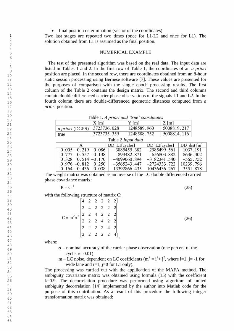
The test of the presented algorithm was based on the real data. The input data are

listed in Tables 1 and 2. In the first row of Table 1, the coordinates of an a priori

position are placed. In the second row, there are coordinates obtained from an 8-hour

static session processing using Bernese software [7]. These values are presented for

the purposes of comparison with the single epoch processing results. The first

column of the Table 2 contains the design matrix. The second and third columns

contain double differenced carrier phase observations of the signals L1 and L2. In the

fourth column there are double-differenced geometric distances computed from a

priori position.

Table 1. A priori and ‘true’ coordinates

X [m] Y [m] Z [m]

a priori (DGPS)

true

Table 2 Input data

A DD_L1[cycles] DD_L2[cycles] DD_dist [m]

The weight matrix was obtained as an inverse of the LC double differenced carried

phase covariance matrix:

P = C-1

(25)

with the following structure of matrix C:

,

(26)

where:

– nominal accuracy of the carrier phase observation (one percent of the

cycle, =0.01)

m – LC noise, dependent on LC coefficients (m2 = i

2+ j

2, where i=1, j= -1 for

wide lane and i=1, j=0 for L1 only).

The processing was carried out with the appllication of the MAFA method. The

ambiguity covariance matrix was obtained using formula (15) with the coefficient

k=0.9. The decorrelation procedure was performed using algorithm of united

ambiguity decorrelation [14] implemented by the author into Matlab code for the

purpose of this contribution. As a result of this procedure the following integer

transformation matrix was obtained:

2 2

4 2 2 2 2 2

2 4 2 2 2 2

2 2 4 2 2 2C m

2 2 2 4 2 2

2 2 2 2 4 2

2 2 2 2 2 4

1 2 3 4 5 6 7 8 9 10 11 12 13 14 15 16 17 18 19 20 21 22 23 24 25 26 27 28 29 30 31 32 33 34 35 36 37 38 39 40 41 42 43 44 45 46 47 48 49 50 51 52 53 54 55 56 57 58 59 60 61 62 63 64 65

(27)

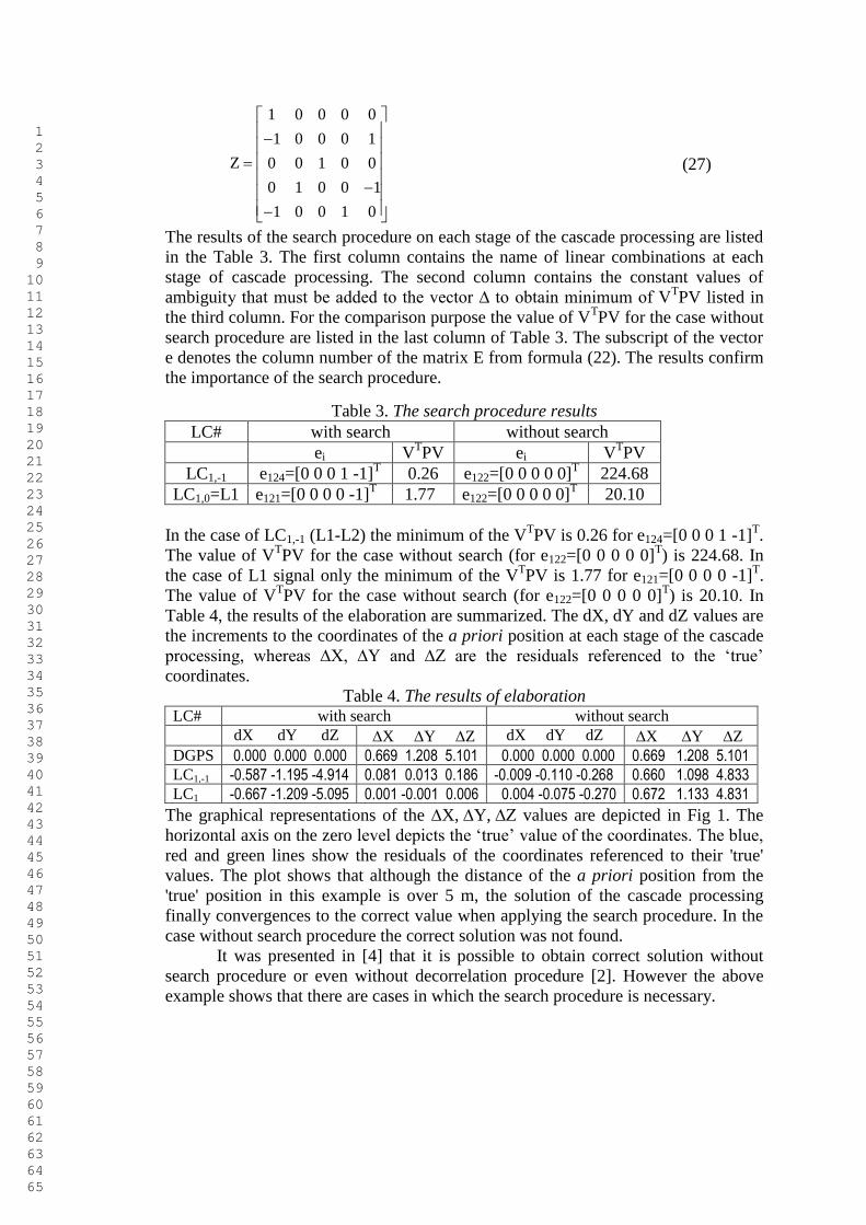
The results of the search procedure on each stage of the cascade processing are listed

in the Table 3. The first column contains the name of linear combinations at each

stage of cascade processing. The second column contains the constant values of

ambiguity that must be added to the vector ∆ to obtain minimum of VTPV listed in

the third column. For the comparison purpose the value of VTPV for the case without

search procedure are listed in the last column of Table 3. The subscript of the vector

e denotes the column number of the matrix E from formula (22). The results confirm

the importance of the search procedure.

Table 3. The search procedure results

LC# with search without search

ei VTPV ei V

TPV

LC1,-1 e124=[0 0 0 1 -1]T 0.26 e122=[0 0 0 0 0]

T 224.68

LC1,0=L1 e121=[0 0 0 0 -1]T 1.77 e122=[0 0 0 0 0]

T 20.10

In the case of LC1,-1 (L1-L2) the minimum of the VTPV is 0.26 for e124=[0 0 0 1 -1]

T.

The value of VTPV for the case without search (for e122=[0 0 0 0 0]

T) is 224.68. In

the case of L1 signal only the minimum of the VTPV is 1.77 for e121=[0 0 0 0 -1]

T.

The value of VTPV for the case without search (for e122=[0 0 0 0 0]

T) is 20.10. In

Table 4, the results of the elaboration are summarized. The dX, dY and dZ values are

the increments to the coordinates of the a priori position at each stage of the cascade

processing, whereas ∆X, ∆Y and ∆Z are the residuals referenced to the ‗true‘

coordinates.

Table 4. The results of elaboration

LC# with search without search

dX dY dZ X Y Z dX dY dZ X Y Z

DGPS 0.000 0.000 0.000 0.669 1.208 5.101 0.000 0.000 0.000 0.669 1.208 5.101

LC1,-1 -0.587 -1.195 -4.914 0.081 0.013 0.186 -0.009 -0.110 -0.268 0.660 1.098 4.833

LC1 -0.667 -1.209 -5.095 0.001 -0.001 0.006 0.004 -0.075 -0.270 0.672 1.133 4.831

The graphical representations of the X,Y, values are depicted in Fig 1. The

horizontal axis on the zero level depicts the ‗true‘ value of the coordinates. The blue,

red and green lines show the residuals of the coordinates referenced to their 'true'

values. The plot shows that although the distance of the a priori position from the

'true' position in this example is over 5 m, the solution of the cascade processing

finally convergences to the correct value when applying the search procedure. In the

case without search procedure the correct solution was not found.

It was presented in [4] that it is possible to obtain correct solution without

search procedure or even without decorrelation procedure [2]. However the above

example shows that there are cases in which the search procedure is necessary.

1 0 0 0 0

1 0 0 0 1

Z 0 0 1 0 0

0 1 0 0 1

1 0 0 1 0

1 2 3 4 5 6 7 8 9 10 11 12 13 14 15 16 17 18 19 20 21 22 23 24 25 26 27 28 29 30 31 32 33 34 35 36 37 38 39 40 41 42 43 44 45 46 47 48 49 50 51 52 53 54 55 56 57 58 59 60 61 62 63 64 65

with search without search

Fig. 1. Residuals of the position coordinates referenced to their ‗true‘ values

TESTS

In order to test the efficiency of the proposed algorithm, the real GPS data of three

baselines were used. Test surveys were performed on December 9th, 2008, on 1.5

km, 9.5 km and 29.1 km baselines, the data were collected with a 30-second

sampling rate. Data sets of each baseline consisted of 120 epochs. The data were

processed according to the proposed approach independently for each epoch. The

ambiguity covariance matrix was formed according to formula (15), as a basis for the

decorrelation procedure. The ―true‖ coordinates were derived using Bernese software

based on an 8-hour data set. Figures 2, 3 and 4 present the results of 120 single epoch

sessions processing the 1.5 km, 9.5 km and 29.1 km baselines. The blue lines depict

the linear residuals of the position obtained from single epoch processing, with

respect to the ―true‖ position from Bernese. The residuals were computed as:

, where ∆X, ∆Y and ∆Z are components of the residuals with

respect to the ―true‖ position. The red lines depict the linear residuals of the a priori

position, with respect to the ―true‖ position.

Fig. 2. Linear residuals of the a priori and final position for baseline 1.5 km

DGPS L1-L2 L10

1

2

3

4

5

X

Y

Z

Residuals of the position coordinates referenced to their 'true' values

X

Y

Z

DGPS L1-L2 L10

1

2

3

4

5

X

Y

Z

Residuals of the position coordinates referenced to their 'true' values

X

Y

Z

2 2 2dV X Y Z

10 20 30 40 50 60 70 80 90 100 110 120-1

-0.8

-0.6

-0.4

-0.2

0

0.2

0.4

0.6

0.8

1

baseline 1.5 km

epoch

Vd [m

]

linear disclosure of the final position

linear disclosure of the a'priori position

1 2 3 4 5 6 7 8 9 10 11 12 13 14 15 16 17 18 19 20 21 22 23 24 25 26 27 28 29 30 31 32 33 34 35 36 37 38 39 40 41 42 43 44 45 46 47 48 49 50 51 52 53 54 55 56 57 58 59 60 61 62 63 64 65

Fig. 3. Linear residuals of the a priori and final position for baseline 9.5 km

Fig. 4. Linear residuals of the a priori and final position for baseline 29.1 km

In most cases, a priori position was farther than 1m from the ‗true‘ position. There

were 109 correct (correct values of the ambiguities and at the same time linear

residuals less than 10 cm) among all 120 solutions (90.8%) in the case of 1.5 km

baseline. There were 105 correct among all 120 solutions (87.5%) for 9.5 km

baseline. In the case of the longest in the test baseline (29.1 km) there were 95

(79.1%) correct among all 120 solutions.

CONCLUSIONS

The MAFA method was improved with implementing a search procedure. The

detailed algorithm of such procedure was elaborated and presented in this paper. The

computational process allows obtaining precise position even on the basis of only

single observational epoch. The results of the tests show the usefulness of the

proposed solutions. The high efficiency of the proposed algorithm was confirmed by

tests performed for short and medium baselines (shorter than 30 km). The number of

10 20 30 40 50 60 70 80 90 100 110 120-1

-0.8

-0.6

-0.4

-0.2

0

0.2

0.4

0.6

0.8

1

epoch

Vd [m

]

baseline 9.5 km

linear discolsures of the final position

linear discolsures of the a'priori position

10 20 30 40 50 60 70 80 90 100 110 120-1

-0.8

-0.6

-0.4

-0.2

0

0.2

0.4

0.6

0.8

1

epoch

Vd [m

]

baseline 29.1 km

linear disclosures of the final position

linear disclosures of the a'priori position

1 2 3 4 5 6 7 8 9 10 11 12 13 14 15 16 17 18 19 20 21 22 23 24 25 26 27 28 29 30 31 32 33 34 35 36 37 38 39 40 41 42 43 44 45 46 47 48 49 50 51 52 53 54 55 56 57 58 59 60 61 62 63 64 65

correct single-epoch solutions varied from 79% to over 90% depending on the

baseline length. Future research will include application of the presented

methodology to multi-station positioning, as literature suggest [8] that this may

further increase success rate of the single epoch solutions.

References

1. Bakuła M., 2010. Network Code DGPS Positioning and Reliable Estimation of

Position Accuracy, Survey Review, 42 (315): 82-91.

2. Cellmer S., Wielgosz P., Rzepecka Z., 2010. Modified ambiguity function

approach for GPS carrier phase positioning, Journal of Geodesy, Vol. 84, 264-275.

3. Cellmer S., 2011a. The real time precise positioning using MAFA method, The 8th

International Conference ENVIRONMENTAL ENGINEERING, selected papers, Vol.

III, Vilnius, 1310-1314.

4. Cellmer S., 2011b. Using the Integer Decorrelation Procedure to increase of the

efficiency of the MAFA Method, Artificial Satellites, Vol. 46, No. 3, 103-110.

5. Cellmer S., 2011c. A Graphic Representation of the Necessary Condition for the

MAFA Method. Transactions on Geoscience and Remote Sensing vol. 50 Issue 2, pp.

482 - 488

6. Cellmer S., 2012. On-the-fly ambiguity resolution using an estimator of the

modified ambiguity covariance matrix for the GNSS positioning model based on

phase data Artificial Satellites (accepted for publication)

7. Dach R., Hugentobler U., Fridez P., Meindl M., 2007. BERNESE GPS Software

Version 5.0., Astronomical Institute, University of Berne

8. Grejner-Brzezinska D.A., Arlsan N., Wielgosz P., Hong C.-K., 2009. Network

Calibration for Unfavorable Reference-Rover Geometry in Network-Based RTK:

Ohio CORS Case Study, Journal of Surveying Engineering, Vol. 135, Issue 3, pp.

90-100

9. Han S. and Rizos C., 1996. Improving the computational efficiency of the

ambiguity function algorithm. Journal of Geodesy 1996, Vol. 70, No. 6, 330-341.

10. Hassibi A, Boyd S., 1998. Integer parameter estimation in linear models with

applications to GPS. IEEE Trans Signal Proc 46: 2938–2952

11. Hofmann-Wellenhof B, Lichtenegger H, Wasle E., 2008. GNSS-Global

Navigation Satellite Systems - GPS, GLONASS, Galileo & more, Springer-Verlag

Wien

12. Jung J. and Enge P., 2000. Optimization of Cascade Integer Resolution with

Three Civil GPS Frequencies Proc. ION GPS’2000, Salt Lake City, September 2000

13. Leick A., 2004. GPS Satellite Surveying. 3rd

edition, John Wiley and Sons, Inc.

14. Liu LT., Hsu HT., Zhu YZ., Ou JK., 1999. A new approach to GPS ambiguity

decorrelation. Journal of Geodesy 73:478–490

15. Teunissen P JG., 1995. The least-squares ambiguity decorrelation adjustment: a

method for fast GPS integer ambiguity estimation, Journal of Geodesy , 1995, Vol.

70, 65-82.

16. Teunissen PJG. and Kleusberg A., 1998. GPS for Geodesy, Springer — Verlag,

Berlin Heidelberg New York, 1998

17. Wielgosz P., 2011. Quality assessment of GPS rapid static positioning with

weighted ionospheric parameters in generalized least squares, GPS Solutions Vol. 15,

Issue 2, April 2011, 89-99

18. Xu P., 2001. Random simulation and GPS decorrelation. Journal of Geodesy

75:408–423

1 2 3 4 5 6 7 8 9 10 11 12 13 14 15 16 17 18 19 20 21 22 23 24 25 26 27 28 29 30 31 32 33 34 35 36 37 38 39 40 41 42 43 44 45 46 47 48 49 50 51 52 53 54 55 56 57 58 59 60 61 62 63 64 65