Long-term return reversals—Value and growth or tax? UK evidence

Electronic copy available at: http://ssrn.com/abstract=1343737

1

Long-Term Return Reversals –Value and Growth or Tax? UK Evidence

By

Yuliang Wu* and Youwei Li

Abstract

This paper examines (i) whether value-growth characteristics have more power than past

performance in predicting return reversals; and (ii) whether typical rational behaviour such as

incentives to delay paying capital gain taxes can better explain long-term reversals than past

performance. We find that value-growth characteristics generally provide better explanations for

long-term stock returns than past performance. The evidence also shows that winners identified

by capital gains dominate past performance winners in predicting reversals in the cross-sectional

comparison. However, in the time-series analysis, when returns on capital gain winners are

adjusted by the Fama and French (1996) risk factors, the predictive power of capital gain winners

disappears. Our results show that capital gain winners are heavily featured as growth stocks.

Return reversals in capital gain winners potentially reflect market price corrections for growth

stocks. We conclude that investors’ incentives to delay paying capital gain taxes cannot fully

rationalise long-term reversals in the UK market. Our results also imply that the long-term return

pattern potentially reflects a mixture of investor rational and irrational behaviour.

Keywords: long-term reversals, overreaction, taxes, UK stock market

JEL classification codes: G11 G14

Both Wu and Li are from Queen’s University of Belfast, 25 University Square, BT7 1NN,

Belfast, Northern Ireland. Wu is correspondent author. E-mail: [email protected] ; Tel: 0044-28-

90973279; Fax: 0044-28-90975156

Acknowledgement

Earlier versions of this paper were present at Queen’s University Belfast and the 16th annual conference of Multinational Finance Society in Crete, Greece. The comments of Donal McKillop, Michael Moore, Khelifa Mazouz, Colin O’Hare, Shuxing Yin, and conference and seminar participants on earlier versions of the paper are gratefully acknowledged.

mailto:[email protected]

Electronic copy available at: http://ssrn.com/abstract=1343737

2

1. Introduction

The evidence of long-term stock return reversals has been found across a wide range of

developed and developing markets (Antoniou et al., 2005; Bhojraj and Swaminathan, 2006;

Chou et al., 2007; Dissanaike and Lim, 2010; Gupta et al. 2010, McInish et al., 2008; Nam et al.

2003; Wongchoti and Pyun, 2005). While the outperformance of loser stocks relative to winner

stocks is generally accepted, indentifying causes of return reversals has been more controversial.

Since the seminal findings of DeBondt and Thaler (1985), Daniel et al. (1998), Barberis et al.

(1998) and Hong and Stein (1999) invoke psychological evidence to motivate a price

overreaction hypothesis in line with a general prediction of the behavioural decision theory of

Kahneman and Tversky (1982). In contrast to the behavioural view of over-reaction, Klein (1999;

2001), George and Hwang (2007) and Grinblatt and Moskowitz (2004) contend that the effect of

losers outperforming winners is attributable to investor rational behaviour such as strategic tax-

avoidance incentives. Lewellen and Shanken (2002) and Brav and Heaton (2002) provide

Bayesians learning models to support rational explanations for long-term reversals. In their

models, investors put too much weight on extreme observations that may generate over-reaction

in beliefs to good and bad news. Reversals occur when investors learn that they over-reacted in

the past. Fama and French (1993; 1996) contend that the long-term winner-loser effect is within

the value-growth paradigm, reflecting that losers are riskier than winners in terms of distress

costs. Consistent with this, Fama and French (1995) show that a high book-to-market equity ratio

as a proxy for high distress costs predicts poor future earnings. Fama (1998), Fama and French

(2006) and La Porta (1996) claim that long-term contrarian performance is the result of a mis-

measured relationship between risk and return1. However, Lakonishok et al. (1994) find that

value stocks outperform growth stocks because of investors over-estimating future growth rates

of growth stocks relative to value stocks. Lakonishok et al. (1994) contend that the value

premium is a mispricing effect rather than a risk measure in Fama and French (1993, 1996).

1 Zhang (2005) provides theoretical models to support this view. Hahn and Lee (2006) and Petkova (2006) also support the view that the HML factor (the value factor) is a potential proxy for business cycle and should be priced in cross-sectional stock returns.

3

To summarize, there are three competing explanations for long-term return reversals. 2 The

behavioural explanations are centred on whether over-reaction to past performance contributes to

return reversals. One of the rational explanations attributes reversals to tax-avoidance incentives,

while it is still controversial whether stock value and growth features reflect risk or mispricing.

This paper seeks to test these three competing explanations by using data of 1673 stocks listed on

the London Stock Exchange (LSE) from 1974 to 2009. By using past performance based winners

and losers as benchmark portfolios, the value-growth hypothesis expects that firm specific

features should have stronger power than past performance in predicting returns. Three variables

are employed as proxies for firm value-growth features, namely book-to-market, cash-flow-to-

price, and earnings-to-price. The capital gain lock-in hypothesis is built upon the idea that winner

reversals are due to investor incentives to delay paying capital gain taxes and winners identified

by capital gains should predict reversals other than past performance winner3. Taxation is one of

the most prevalent market frictions in financial markets, affecting investment decisions and

distorting the valuation of assets (Constantinides, 1984). However, empirical evidence on the

relationship between tax and asset price is predominantly limited in the U.S. The UK is also a

country with legal settings on capital gain taxes and one of our purposes is to test whether capital

gain taxes can ultimately affect long run asset prices in a similar pattern as those documented in

the U.S. To our best knowledge, the capital gain lock-in hypothesis to explain long-term

reversals have not been examined in the UK context.

Previous studies on long-term reversals mainly focus on the profitability of contrarian strategies

in which value and growth features associated with winners and losers are obtained from the

factors loadings on the relevant asset pricing models (e.g. the CAPM and the Fama-French

model). We pair-wisely compare returns on portfolios which are formulated on past performance,

tax incentives and firm specific value-growth features, in the Fama-MacBeth (1973) regressions

on a head-to-head basis. This approach is different from those customarily adopted in the

literature.

2 Conrad et al. (2003) and Conard and Kaul (1993) suggest that evidence of long-term reversals may be a

consequence of data snooping.

3Similarly, loser reversals are caused by tax-loss selling at tax year ends, and this is strongly linked with the calendar effect. However, this paper mainly investigates the capital gain lock-in hypothesis.

4

To pre-empt our results, we find that firm value-growth features generally provide better

explanations for cross-sectional stock returns than past performance in the long term. The

predictability of value-growth features is relatively strong when we use book-to-market equity

ratio as a proxy for value-growth features. Our striking results are from the comparison between

past performance and capital gain measures. In the cross-sectional analysis, we find that winners

identified by a large amount of capital gains completely dominate past performance winners in

predicting reversals. In the time-series analysis, the predictive power of capital winners cannot

be fully explained away by using the market and the two-factor (market and size) model.

However, inconsistent with the findings in the U.S. (George and Hwang, 2007), the predictive

power of capital gain winners becomes disappeared in the three-factor model (FF) (Fama and

French, 1993; 1996). Our results show that capital gain winners are heavily featured as growth

stocks, which are more likely to be overvalued than value stocks. The evidence suggests that the

reversals in stocks with large amounts of capital gains potentially reflect market price corrections

for growth stocks. Therefore, we conclude that incentives to delay paying capital gain taxes are

less likely to explain long-term reversals in the UK context. This paper empirically tests both the

typical rational incentives based on deferral tax payments and the classical past performance

based behavioural explanations for long-term return reversals. The results suggest that neither of

them win this game. Overall, we conjecture that the pattern of return reversals potentially reflect

a mixture of investor rational and irrational behaviour.

The rest of the paper is organized as follows: Section 2 reviews the literature. The hypotheses are

developed in section 3, while section 4 outlines the sample and the methodology. Section 5

reports the empirical results. Finally, section 6 provides conclusions and implications of the

paper.

2. Literature Review

Since the seminal finding of DeBondt and Thaler’s (1985) that past losers outperform past

winners over 3 to 5 years, considerable academic effort has sought to explain this winner-loser

effect. Early research argues that time-varying beta risk explains this return reversal pattern

(Chan, 1988; Ball and Kothari, 1989; Jones, 1993). However, Lee and Swaninathan (2000) and

Jegadeesh and Titman (2001) contend that the contrarian strategy by buying losers and selling

5

winners offers superior risk-adjusted performance. Outside the conventional risk-return paradigm,

Daniel et al. (1998) attribute long-term and short-term return anomalies to investor

overconfidence and self-attribution, while Barberis et al. (1998) introduce psychological

concepts of “the representativeness heuristic” and “the conservatism bias” which investors

inherently experience when interpreting new information. The two behaviour models indicate

that investor initial underreaction to news causes momentum. When investors correct their priors,

they will experience overreaction in the long term. In the behavioural view, under-reaction in the

short run and over-reaction in the long run are more likely to be an integral process by which the

market absorbs new information. The evidence of return momentum in Jegadeesh and Titman

(1993) and reversals in the long run (Jegadeesh and Titman, 2001) is consistent with this

contention. However, George and Hwang (2004) find that there is no direct link between

momentum and reversals, since momentum captured by the relative price to 52-week high price

has no long-term reversals4.

In terms of rational explanations of return reversals, Constantinides (1984) first develops the tax

timing option model for the abnormal January returns. In his model, investors should realize

capital losses as soon as they occur; since capital losses can offset future realized capital gains.

In contrast to capital loss, Kleim (1999; 2001) models that investors should have great incentives

to delay realising embedded capital gains, unless buyers can offer a higher price to compensate

sellers for some costs of capital gain taxes. When stocks are eventually sold to buyers without

any embedded capital gains, prices of those stocks will go down, leading to winner reversals.

The two tax-based models predict that stock returns should exhibit reversals in the long term, if

investors take into account of potential capital gain tax payment. Shackelford and Verrecchia

(2002) develop a trading model in which rates of capital gain tax create a trade-off between

optimal risk-sharing and optimal tax related trading. They show that sellers are reluctant to sell

appreciated assets sooner because they are subject to higher capital gains taxes. In order to

acquire stocks, buyers must provide compensation in the form of higher sales prices to sellers.

On the empirical side, Grinblatt and Moskowitz (2004) find no reversals for consistent winners

4 However, Gupta et al. (2010) investigate the 52-week high measures in international stock markets of 51 countries and find that momentum profits also exhibit reversals after the first 12 months holding period.

6

(identified as the cumulative return from months t-36 to t-13), while consistent losers have no

significant reversals outside January, suggesting that reversals are caused by tax-loss selling

consistent losers at tax year ends. In a similar spirit, George and Hwang (2007) provide empirical

evidence in support of the model of Kleim (1999) with the role of capital gains in reversals. They

find that losers reverse their returns only in January, while winner reversals are attributable to

investor incentives to delay paying capital gain tax. Therefore, the evidence in U.S supports tax-

motivated explanations for reversals.5

Since Fama and French (1993) develop the three-factor model, the debate on the long-term

return anomaly shifts to firm value-growth characteristics (e.g. book-to-market ratio, cash-flow

to price ratio, and earnings to price ratio). While stocks with a high book-to-market ratio possibly

signals a high distress cost, losers should have a high expected return relative to winners that

have on average a low distress cost. Consistent with this, Fama and French (1995) show that high

book-to-market equity ratio predicts poor future earnings. Zhang (2005) ’s theoretical model

supports Fama and French’s conclusions providing an analytical framework in which value

stocks additional riskiness emanates from their inability to scale down capital investment during

market downturns. By using indexes to rank firms by default probability or intensity of distress,

Garlappi et al. (2008) and Chava and Purnanandam (2010) confirm the findings of Fama and

French (1995) and Zhang (2005) that distress costs do predict defaults for individual firms and

they are larger during recessions. The above authors support that the value premium potentially

represents risk. However, Ang and Chen (2007) challenge the risk argument of the value

premium and they find that the CAPM captures the value premium during 1926-1963 in the U.S.

Lakonishok et al. (1994) and Daniel and Titman (1997) conclude that value out-performs growth

and that this finding may be explained by market participants’ consistently over-estimating

future growth rates of growth stocks relative to value stocks and that the return to value investing

is no riskier than growth strategies.

5 Dai et al. (2008) find that investors require higher prices to sell stocks after the Taxpayer Relief Act of 1997 in the U.S. This evidence is consistent with the capital gain lock-in effect. Jin (2006) investigates whether the capital gain tax is an impediment to selling and he finds that selling decisions are negatively influenced by an amount of cumulative capital gains for institutional investors, who have a large number of tax-sensitive clients.

7

Most studies of the UK market have extensively analysed long-term contrarian investment

strategies, but main sources of long-term contrarian performance are not agreed. Clare and

Thomas (1995) first investigate long-term reversals for a sample of 1000 UK stocks from 1955

to 1990. They support the over-reaction hypothesis and attribute their findings to a size effect.

However, Dissanaike (1999) finds reversals are not driven by a size effect for a sample of FTSE

500 firms from 1975-1991. Galariotis et al. (2007) provide evidence supporting profitable

contrarian investment strategies for the London Stock Exchange (LSE) listed stocks from 1964 to

2005. They conclude that the Fama-French (1993) model accounts for all contrarian profits.

Regarding to the value-growth features, Li et al. (2009) analyze the value premium and find that

high return volatility is one of possible causes for the superior performance of value stocks in the

UK from the 1963 to 2006 period. Recently, Dissanaike and Lim, (2010) investigate contrarian

strategies by incorporating the accounting information based upon the Ohlson (1995) and the

residual income model. They find that the accounting information based contrarian strategies

cannot outperform the BM (book-to-market) based contrarian strategies.

So far there is no consensus on causes of long-term return reversals, are long-term reversals

driven by past performance (e.g. losers and winners), firm value-growth characteristics, or

investor tax incentives? This paper empirically answers this question.

3. Hypothesis Development

To investigate the three competing explanations, we formulate the value-growth hypothesis and

the capital gain lock-in hypothesis, while the null hypothesis that past performance predicts

return reversals is set as the benchmark explanation. We make two comparisons, (i) past

performance against value-growth and (ii) past performance against capital gains.

3.1 Value-growth hypothesis

Value investing is an important strategy to exploit current out of favour stocks with market

participants. Value investors believe that the book value of a firm’s equity is a useful barometer

of intrinsic value. High book-to-market (value) stocks are likely to be undervalued, while low

book-to-market (growth) stocks are likely to be overvalued. Consistent with this, Fama and

8

French (1992, 1993) confirm that high book-to-market (henceforth BM) earn significantly higher

average returns than low BM stocks in the U.S stock markets. In relation to long-term reversals,

the findings of Fama and French (1996) show that the Fama-French (1993) factors explain the 1-

month-ahead returns of long-term (5 years) winners and losers. The factor loadings in the FF

model indicate that winners (losers) are more likely to be growth (value) stocks. Fama and

French (2006) claim that the return premium to value stocks potentially represents compensation

for another dimension of systematic risk in addition to beta. Our first hypothesis, the value-

growth hypothesis, is built upon the simple idea that the value-growth strategy should be more

powerful in predicting returns than the winner-loser strategy. We expect that losers and winners

gain insignificant returns.

3.2 Capital gain lock-in hypothesis

The tax related explanations for reversals is modelled on the ground that general tax law settings

have limited abilities to recognize capital loss. If an investor incurs any capital loss in previous

tax-year, the amount of loss has a “carry-over” feature which can offset current or future capital

gains. In the U.S markets, losers have significantly positive returns in January. This evidence is

consistent with the notion that investors exploit losers to establish tax-loss positions at the tax

year end. The logic for winner reversals is built upon the idea that capital gain taxes are paid

only when gains are realised. Investors will only sell winner stocks with a large embedded gain

when prices can compensate them to forgo the value of delaying payment of tax. When winners

are eventually sold to buyers without large embedded gains, the marginal investor’s reservation

prices fall. This process leads to winner reversals. The capital gain lock-in hypothesis claims that

stocks with a large amount of capital gains should reverse their returns in the long term. George

and Hwang (2007) is the first to test this hypothesis in the contexts of the U.S and the Hong

Kong markets. They find that embedded capital gains are responsible for winner reversals in the

U.S but not in Hong Kong. The latter market has no legal settings of capital gain taxes. We

follow George and Hwang (2007) to build upon capital gain measures and to see whether these

measures have any dominant predictive power over winners identified by past performance.

4. Data and Methodology

4.1 Data

9

The sample of stocks is based on the constituents of the FTSE-All Share Index in the London

Stock Exchange (LSE) from June 1974-December 2009. Monthly prices and firm characteristics

(MV, BM, CF/P and E/P) of each stock are extracted from the Thomson Datastream (TD). Since

the TD may contain incorrect data information (Ince and Porter, 2006), we undertake three clean-

up procedures for the dataset to ensure the validity and consistency of the sample dataset. This

practice is in line with Ince and Porter (2006). First, the TD records the most recent price for the

full time series if a stock is delisted during the sample period. To eliminate this dummy record,

we re-code the monthly return series as missing values from the end of the sample period back to

the first nonzero return6. Second, Ince and Porter (2006) find that the TD includes stocks which

are not listed on the LSE. We search for the stock exchange in which a stock is listed and

exclude those which are not listed in the LSE. In addition, we screen all constituent stocks and

exclude those whose quoted prices are not denominated in the British Sterling. Finally, we

exclude unit trusts, close-end, and open-end funds in the sample7. Our sample dataset contains

1673 sample stocks and 332,220 firm-month observations. If a stock has less than 60-month

price information, this stock is also excluded from analysis. The dataset is unbalanced in each

calendar month, meaning that the number of observations varies when we run calendar time

based Fama-MacBeth (1973) regressions. With a 60-month test period, the first cross-sectional

regression starts from June 1979, while the last regression ends in December 2009.

4.2 Variables Description

6 Additionally, we use a variable TIME provided by the TD to find the date of last equity price data for delisted stocks. However, we find that the value of TIME is not informative for delisted stocks. For example, the value of TIME is “#NA” for the Manchester United Football Club, which was delisted in May 2005. This procedure to record the return series as missing values is the same as that used by Ince and Porter (2006).

7 Since these stocks have no information on book value per share or earnings per share in the TD, they can be easily identified in the dataset.

10

(i) Past performance measure (5year winner or loser8): this measure is simply the stock’s return

over the portfolio formation period, 60

60

jt

jtjt

P

PP( )60...3,2,1j . The subscript j is the number

of rolling back windows. The subscript t denotes month t.

(ii) Value-growth characteristics: we use three firm ratios to capture value-growth features. BM

is the book to market ratio defined as book value equity (BV) divided by market value equity

(MV). Following Fama and French (2006), we record BM as a missing value if it is negative.

CF/P is a cash flow to price ratio defined as operational cash flows divided by price. E/P is an

earning price ratio defined as earnings divided by price. The numerators of the three ratios, BV,

CF, and E, are fiscal year ending values in the preceding calendar month t-j. The denominators

of the three ratios, MV and P, are values in month t-j.

(iii) Capital gain measures: we follow George and Hwang (2007) to formulate two measures for

capital gains.

(a) Five-Year Low Measure (FYL): this measure gives the nearness of the month t-j price

to the stock’s 5-year low:

)(1 60

160

1

n njt

njtjtnjt

nnjt

jt P

PPw

wFYL (j=1, 2, 3, … 60) (1)

where wt-j-n is a dummy variable with a value of one if Pt-j-n=min {Pt-j , Pt-j-1 ,…, Pt-j-60}

and zero otherwise. FYL is a measure of embedded capital gains under the extreme

assumption that stocks are bought at the 5-year lowest. With ex post, FYL measures the 8 In the literature of long-term return reversals, documented abnormal returns seem to be less sensitive to the length

of portfolio formation period. DeBond and Thaler (1985) find the contrarian performance is 31.9% over the 5-year period (0.53% per month) according to the past 5-year return sorting and is 24.6% over the 3-year period (0.68% per month) according to the past 3-year return sorting. In the unreported table, we calculate the correlations between winners and losers according to different portfolio formation periods (e.g. 3-year and 4-year). 5-year winner correlates more with 4-year winner and relatively less with 3-year winner, specifically, 0.72 for the former and 0.58 for the latter. There is a similar correlation pattern for losers. The correlation matrix shows that even though we use different time horizons to define winners or losers, there is a great magnitude of similarity in past performance. For instance, 5-year winners and 3-year winners have 58% (more than 50%) of similarity in terms of their past performance.

11

maximum potential capital gains. The capital lock-in hypothesis therefore predicts that

stocks identified as winners based on a ranking by FYL will experience negative excess

returns.

(b) Equal-weighted gain only measure (EWGO): This measure equals to

(2)

where njtw is a dummy variable with a value of one if Pt-j >Pt-j-n and wt-n=0 otherwise.

This measure recognises capital gains only during the past 60 months, while it also

assumes that capital losses cannot generate potential benefits of deferral capital gain tax

payments. According to the capital lock-in hypothesis, winners identified by this measure

should exhibit stronger reversals than past performance winners. However, losers

classified by this measure indicate that they have a less amount of capital gains and,

therefore, should have no reversals.

(iv) Momentum controls (the 52 Week high price): To control for the momentum effect, we use

dummies of 52wkhWi,t-j and 52wkhLi,t-j which are the highest and lowest price levels in the 52

weeks. Following George and Hwang (2004), we set 52wkhWi,t-j (52wkhLi,t-j) to one if jti

jti

high

P

,

, is

ranked among the top (bottom) 30% of all stocks in month t-j, and zero otherwise. Here, Pi,t-j is

the price stock i at the end of month t-j and highi,t-j is the highest month-end price of stock i

during the 12-month period that ends on the last day of the month t-j . George and Hwang (2004)

find the 52-week high measure is more able to capture short-term momentum than the past

performance measure based on the fixed (e.g. 6-month returns) window used by Jagadeesh and

Titman (1993)9. Furthermore, George and Hwang claim that the 52-week high measure is not

subject to long-term reversals.

9 In addition, George and Hwang (2004) find that the 52-week high measure is superior to Moskowitz and Grinblatt (1999) who argue that momentum in individual stock returns is driven by momentum in industry returns.

60

160

1

),60,...2,1)((1

n jt

njtjtnjt

nnjt

jt jnP

PPw

wEWGO

12

Our ranking rule follows George and Hwang (2004, 2007) and Grinblatt and Moskowitz (2004)

with a 30% cutoff rate for each variable. We set two dummies for past performance. 5year loser

(winner) equal 1 if a stock’s past performance is in the top (bottom) 30% of all stocks at month t-

j and zero otherwise. There are also four dummies for each capital gain measure, for example,

EWGO winner, EWGO loser, FYL winner and FYL loser. EWGO (FYL) winner (loser) equals 1 if

a stock is ranked in the top (bottom) 30% of stocks in terms of EWGO (FYL) at month t-j.and

zero otherwise. The same settings are applied to firm ratio variables, BM, CP/P and E/P. For

example, HBM (LBM) equals 1 if a stock is ranked the top 30% of all stocks in terms of BM at

month t-j.

4.3 Empirical model

We use the Fama and MacBeth (1973) regressions to estimate abnormal returns for each

portfolio. If an investor forms portfolios of winners and losers every month and hold these

portfolios for the next T months, the return earned in a given month t is the equal-weighted

average of the returns to T portfolios, each formed in one of the past T months t-j (for j=1,...,T

and T=1,.. 60). The denotation j is a subscript of the number of rolling back months. The

contribution of the portfolio formed in month t-j to the month t return can be obtained by

estimating the following cross-sectional regression,

ijtjtijtjtijt

jtijtjtijttijttijtjtit

eyearLoserbyearWinnerb

wkhLoserbwkhWinnerbsizebRbbR

,6,5

,4,31,21,10

55

5252 (3)

where Rit is the return to stock i in month t. Sizei,t-1 is market capitalisation in a logarithm form

for stock i and at month t-1. Ri,t-1 is stock i’s return at month t-1 . Both Sizei,t-1 and Ri,t-1 are

included in the regression as deviations from cross sectional means at month t-1. The intercept

b0jt is the risk neutral portfolio’s return which has been taken out by the effects of average size,

bid-ask bounce, and momentum. We run this regression 60 times (j=1,2,…60) for each calendar

month t from June 1979 to December 2009. The averaged return for 5-year winners over the 60-

month holding period at month t can be computed as 60

1 55 60

1j jtt bS .Then, the time series

mean, 5S , is an excess return for past winners relative to stocks which are neither winners nor

13

losers. The coefficients on other variables can be computed and interpreted in a same way. The

time series means ( 5S ) of the month-by-month estimates and their t-statistics are reported in the

tables. The 60-month observation window is typically used in the literature of long-term stock

return analysis (Fama and French, 1996; George and Hwang, 2007). The documented short-term

anomaly such as momentum also tends to be reversed in the 5-year period (Jegadeesh and

Titman, 2001). Furthermore, by using the Fama-MacBeth (1973) approach, we examine

abnormal returns not only across the overall 5-year averaged return but also the return in each

sub-interval (e.g. the first, second, third until the fifth year) time period.

We also run Eq (4) to investigate whether long-term returns can be explained by BM ratio.

ijtjtijt

jtijtjtijtjtijt

jtijtjtijttijttijtjtit

eEWGOLoserLBMb

EWGOWinnerHBMbyearLoserbyearWinnerb

wkhLoserbwkhWinnerbsizebRbbR

,8

,7,6,5

,4,31,21,10

)(

)(55

5252

(4)

In Eq (4), HBM and LBM are stocks within the top and bottom 30% of BM in all stocks at month

t-j. According to the value-growth hypothesis, 7b and 8b should be respectively positive and

negative. More importantly, if value-growth characteristics can fully explain long-term returns,

past performance should have no power in predicting returns, suggesting that 5b and 6b are

statistically near to zero. To test the capital gain lock-in hypothesis, we replace the variables of

HBM and LBM in Eq(4) with EWGO winner and loser. If capital gain measures can rationalise

reversals, we should observe that EWGO winners have significant negative returns. However,

returns 5-year winners ( 5b ) become insignificantly different from zero.

Risk-adjusted abnormal returns for each portfolio in Eq (4) are obtained by using the Fama-

French (1993) three-factor model over the holding period. Specifically, the time series of tS5 ,

tS6 , tS7 , and tS8 are individually regressed on the Fama-French (1993) three factors. The

intercepts (alphas) of the regressions are risk-adjusted abnormal returns for 5-year winner, 5-year

loser, high BM (EWGOWinner), and low BM (EWGOLoser) portfolio. The four portfolios in Eq

(4) are associated with two competing long-term investment strategies, for example, past

performance against capital gains, or past performance against BM. To examine the joint

14

significance of returns on the four portfolios, we employ the GRS statistical test developed by

Gibbsons et al. (1989) with the null hypothesis that risk-adjusted abnormal returns on the four

portfolios are jointly equal zero10.

The Fama-MacBeth (1973) methodology is widely used in the empirical finance literature,

however it does not take account of serial correlation across time in the residuals for a given firm,

the firm effect (see, for instance as highlighted by Petersen, 2009), which will generate biased

standard errors. Petersen (2009), Cameron et al. (2006) and Thompson (2010) suggest using

clustered standard errors controlled in two dimensions: time-series and cross-section. However,

as noted by Thompson (2010), the method of clustered standard error works well when the

number of firms and time periods is not too different. If there are far more firms than time

periods, clustering by time eliminates most of the bias unless within-firm correlations are much

larger than with-in time period correlation. Moreover, in this case, double clustering generates

probably less biased, but much noisier standard errors. In our dataset, we have 366 months and

700-800 firms in each month. We implement the method of clustered standard errors and find

that the results are not significantly different from those used by the Fama-MacBeth (1973)

method. Moreover, in the context of this paper, the clustered standard error procedure cannot be

used to generate risk-adjusted returns. While month-by-month abnormal returns calculated by the

Fama-MacBeth (1973) method for each portfolio are regressed on the time-series Fama-French

(FF) three factor model, month-by-month abnormal returns are not obtainable by the clustered

standard error method, which is one single pooled regression. Consequently, we choose in this

paper to utilise the Fama-MacBeth (1973) methodology11.

5. Empirical Results

5.1 Simple correlations

10 The GRS test is basically an F-statistics test on risk-adjusted returns of portfolios. Fama and French (2006) also use the GRS test to evaluate whether the value premium varies with firm size.

11 For interested readers, the results based on the clustered standard error method are available from the authors upon

request.

15

Table 1 reports a correlation matrix for the 14 variables which are calculated as time-series

averages of cross-section correlations. We find that 5-year winners have a positive correlation

(0.11) with 52 week high winners and a negative one (-0.11) with 52 week high losers. This fact

gives a further justification to control for momentum which can potentially offset long-term

return reversals especially in the first year after portfolio formation. The correlation between

EWGO winner and low-BM is almost in a same magnitude as that between 5-year winner and

low-BM (0.27 against 0.24). Furthermore, regardless of past performance and embedded gain

measures, winners have higher (lower) correlations with low (high)-BM, CF/P and E/P than

losers. This may imply that winners share some similar features, even though we have defined

them in a different way.

5.1 Past performance winners and loser

We first estimate average returns for 5-year winners and losers by running the Fama-MacBeth

regressions in each calendar month from 1979-2009. The time-series averages for each

coefficient are reported in Table 2. Following Grinblatt and Moskowitz (2004) and George and

Hwang (2007), we report estimates both including and excluding January and April. This method

reflects the tax setting that the UK personal tax year ends in March12. Column (11) and (12)

show returns related to the entire 5-year holding period, while other columns report returns over

subintervals of the 5-year period. The last row gives averaged observations which are included to

run cross-sectional regressions in each calendar month.

[Insert Table 2 here]

In column (11) and (12), 5-year winners have a significantly negative return of -0.10% outside

January and April, while 5-year losers earn a significantly positive return of 0.12% over a 5-year

horizon. The magnitude of contrarian performance, measured by the return on losers minus

winners, is around 0.21% per month or 2.52% per annum. In each subinterval year, losers begin

to have a positive return of 0.15% in the first year after portfolio formation. The tendency of

losers’ positive returns ends in the fourth year (column (7) and (8)). Winners start to have a

12 Draper and Paudyal (2007) show that 35% of their 1763 sample of UK companies during 1994 had a December year-end and 21% had a March year-end.

16

negative return of -0.10% in the second year (column (3)). The magnitude of winner reversals in

each subinterval year is highly persistent with a range from -0.10% to -0.06% per month. Loser

returns outside January and April are similar to those including all calendar months except the

window of (1, 12) with an insignificant return of 0.07% per month. In other windows including

the entire 5-year window, the difference is relatively small and is only around 3-4 basis points.

Overall, when the results are compared with those in the U.S. markets (George and Hwang,

2007), we find no strong evidence in the UK market to support the January-April effect that is

potentially linked with loser reversals caused by tax-loss selling at the tax year ends.

When we look at control variables: momentum variables (52wkh Winner and 52wkh Losers),

microstructure effects (Ri,t-1), and size, the 52 week high price captures short term momentum.

For winners momentum the return is positive and 0.28% per month (column 1) while for losers it

is negative and 0.48% per month in the first year ((1, 12) month holding period). Consistent with

the finding of George and Hwang (2004), momentum winners and losers do not reverse their

returns in the long term. Our proxy to control for microstructure effects (Ri,t-1) is significantly

and negatively correlated with monthly returns in every holding period. This highlights the need

to control for a negative autocorrelation process between current and previous month return

(Jegadeesh and Titman, 1995).

5.2 Tests of the value-growth hypothesis

We use three firm ratios, BM, E/P, and CF/P as proxies for firm value-growth characteristics.

We compare whether past performance such as winners and losers, or value-growth

characteristics, can better explain long-term returns. We perform three pair-wise comparisons: (i)

high and low BM ratio versus winners and losers, (ii) high and low E/P ratio versus winners and

losers, and (iii) high and low CF/P ratio versus winners and losers. Table 3 report estimates13.


In Panel A, we compare returns between winners and losers and high and low BM ratio stocks.

Consistent with the value-growth hypothesis, high and low BM stocks earn significantly positive

13 Control variables are not reported for the brevity.

17

and negative returns, respectively. In the 5-year period (column 11), high BM stocks have a

return of 0.37% per month while low BM stocks earn a return of -0.21% per month. Over a 5-

year period both 5-year winners and 5-year losers obtain insignificant returns (column 11 and 12).

In each subinterval horizon, there are only two windows in which losers and winners have

significant returns, for instance, 0.14% for losers in the window (37, 48) outside January and

April and -0.12% for winners in the window (49, 60) outside January and April. These results

contrast to winner-loser reversals in Table 2. The evidence suggests that BM ratio is better at

capturing long-term returns than past performance measures.

Panel B of Table 3 compares CF/P and past performance measures. High CF/P stocks have a

significantly positive return of 0.35% per month (column 11) across a 5-year period. However,

low CF/P stocks have a significantly negative return of -0.51% only in the first year (column (1)

and (2)) after portfolio formation. This result implies that CF/P has weaker predictive power than

BM does. Regarding past performance, we find that losers have an insignificant return of 0.07%

per month over a 5-year period (column 11). In each subinterval, average returns for losers are

insignificantly positive in seven out of ten sub-period windows. For winners, we can observe a

negative return of -0.12% per month over a 5-year period. By introducing CF/P into the

regressions, loser reversals have been substantially reduced but there is little effect on winner

reversals.

Panel C of Table 3 compares E/P and past performance measures. Value stocks measured by a

high E/P ratio have large positive returns in the whole 5-year holding period and in the first four

years (column 1 to 8). On average, they can earn 0.41% (column 11) per month relative to the

risk-neutral portfolio over a 5-year period. In contrast, growth stocks with a low E/P ratio have a

negative averaged return of -0.15% per month (column 11) over a 5-year period. These results

are consistent with the value-growth hypothesis. For past performance based winners and losers,

we find that losers’ returns become insignificantly different from zero over a 5-year period. The

negative return of -0.10% for winners is weakly significant at a 10% level.

In summary, value-growth characteristics captured by BM are better at predicting cross-section

stock returns than CF/P and E/P over a long term. The comparison between value-growth and

18

past performance strategies shows that the long-term return pattern is better explained by firm

specific characteristics than by past performance.

5.3 Test of capital gain lock-in hypothesis


We compare past performance and the 5 year low measure in Panel A of Table 4. 5-year low

winners have significantly negative returns in every window except in the first year (1, 12). Over

the whole 5-year period, 5-year low winners have a negative return of -0.13% per month in all

calendar months and -0.21% per month outside January and April. In contrast, past performance-

based winners have no significant returns across each window. This result suggests that capital

gain winners completely dominate past winners to predict reversals. Furthermore, significant

returns on past losers are only observed in windows including January and April, except column

(4).

Panel B in Table 4 reports results of EWGO and past performance measures. The results are very

similar to 5-year low measures. EWGO winners have a significantly negative return of -0.09%

per month over a 5-year period (in column 11) with a t-value 2.01 in all months and -0.15%

outside January and April with a t-value 2.94. EWGO winners largely replace past winners to

predict reversals. In summary, capital gain measures completely dominate past performance

measures in predicting winner reversals in the cross-sectional comparison. These results give

some support to the capital gain lock-in hypothesis.

5.4 Risk-adjusted returns

The purpose of this part of analysis is to see whether abnormal return can be maintained after

risk adjustments. We regress time-series variables (e.g. tS5 ) on the Fama-French (1993) (FF)

factors. The intercepts in the regressions are risk-adjusted returns. The comparison between past

performance and the specific BM ratio is reported in Table 5 14 , while Table 6 shows the

comparison between past performance and embedded capital gain measures.

14 Other pair-wise comparisons (e.g. CF/P against past performance, E/P against past performance) by using the market model, the two-factor model, and the three-factor model are also available upon request.

19


In Table 5, stocks with a high BM ratio earn a significant return of 0.14% per month in all

calendar months (column 11). The size of this positive return is less than half of the abnormal

return reported in Table 3 (0.37%). When excluding April and January in column (12), the return

is 0.21% per month and 0.07% higher than the one in column 11, implying that the high BM

portfolio has a negative return in January and April. This result indicates that value stocks are

less likely to have the January-April effect. In each sub-period, value stocks identified by a high

BM ratio have persistently strong positive returns except the window (48, 60) in columns (9) and

(10). However, low BM stocks have no significant returns either in the window (1, 60) or in each

sub-period. Winners identified by past performance have a return of -0.08% per month during

the 5-year period, while this negative return is only statistically significant at a 10% level. In

contrast, losers have no significantly positive returns through column (1)-(12). The GRS test

rejects the null hypothesis that the four portfolios have an equal return of zero across each

observation window (column 1 to 12). Overall, long-term reversals on past winners and losers

largely disappear after we control for BM, while risk-adjusted abnormal returns on value stocks

are likely to be maintained in the framework of Fama and French (1993).


Panel A in Table 6 compares 5-year low and past performance measures. On a risk-adjusted

basis, 5-year low winners have no significantly negative returns in any horizon. Over a 5-year

period, 5-year low winners have an insignificantly positive return of 0.06% (column 11) per

month. However, 5-year winners have a significantly negative return of -0.09% per month over a

5-year period. The GRS test in column (7) and (8) with the null hypothesis that the four

portfolios jointly have no significant alpha cannot be rejected at a 10% level. The results in

Panel B depict a same picture. While no significantly negative is found for EWGO winners, 5-

year winners have a significantly negative return -0.12% per month over a 5-year period. The

GRS test cannot reject the null hypothesis that returns all equal to zero in column (5)-(8) at a 5%

level or higher. This means in the third and fourth year after portfolio formation, the four

portfolios jointly have no abnormal returns. Overall, the results on the FF model show that

20

embedded capital gain measures lost most of their predictive power against past winners in

predicting reversals.

5.5 Robustness of risk-adjusted abnormal returns

By using abnormal returns and risk-adjusted abnormal returns, we obtain two different pictures

on the predicative power of capital gain measures. To investigate further on why capital gain

measures lost most of their power in predicting winner reversals, we re-estimate risk-adjusted

abnormal returns by using two additional models, namely the market model and the two-factor

model, which includes size and the market factor.

ifmiii eRRbaR )( (5)

iifmiii eSMBsRRbaR )( (6)

iiifmiii eHMLhSMBsRRbaR )( (7)

iR is the averaged 60-month return, which we obtain from the Fama-MacBeth regression in each

calendar month. mR is a market return. SMB and HML are size and value factor, respectively

according to the definitions of Fama and French (1993; 1996) (FF). Table 7 reports the results.

To save space, we only report risk-adjusted abnormal returns over the 60-month period including

all calendar months.


Table 7 provides interesting results for why stocks with a large amount of capital gains

experience negative returns. In the market model, both 5-year low winners and EWGO winners

have significantly positive market loadings (column 1 Panel A and Panel B) (e.g. 0.1842 and

0.1415), suggesting that the two portfolios have a higher market risk than the risk-neutral

portfolio with a zero beta. Thus, their risk adjusted returns should not be higher than those

calculated by the Fama-MacBeth model. In column (1), the two portfolios’ returns are nearly the

same as those in Table 4 (-0.0012 against -0.0013; -0.0009 against -0.0009) with significance

levels less than 10%. Similar results can be found in the two factor model with one additional

21

size factor (column (2)). However, when the value factor is incorporated into the model (column

(3)), significantly negative abnormal returns on the two portfolio become disappeared. This is

because 5-year low and EWGO winners have a negative value loading of 0.3687 and 0.2932,

respectively. More importantly, each of the value loading exceeds the aggregated loadings of the

size and market factor15. Thus, the risk-adjusted returns for the two portfolios in the FF model

should be greater than those in Table 4. Consistent with this, the risk-adjusted returns on the two

portfolios are both insignificantly different from zero (e.g. 0.0004 for 5-year low winners and

0.0006 for EWGO winners). Negative value loadings indicate that stocks with large amounts of

capital gains have a strong growth feature. Relative to value stocks, growth stocks are more

likely to have positive earnings and to be highly priced, leading to a low book-to-market ratio

(market-cap has increased). In addition, these capital gain winners are also small stocks with

positive loadings on the size factor. The intuition behind this finding is that small stocks are

more volatile and they may more easily accumulate capital gains than big stocks. Therefore, our

results suggest that the growth feature is more likely a driving force of return reversals than

capital gains.

The GRS tests in Panel A and Panel B show that in terms of the market model (GRS test (i)) both

capital gain portfolios and past performance portfolios have returns jointly insignificant from

zero. However, in the FF model, the GRS tests (test (iii) in Panel A and B) reject the hypothesis

that capital gain portfolios and past performance portfolios have joint zero returns. Column (9)

reveals that 5-year winners have significantly negative returns after risk adjustments, implying

that capital gain winners have no power over past performance winners to predict return

reversals. In contrast with capital gain winners, the factor loadings imply that past performance

winners are large, low market risk and value stocks. Finally, the adjusted 2R s in column (3) and

(6) in Panel A and Panel B are larger than in other columns, implying that the FF model is better

at capturing the return variations in capital gain portfolios. However, the FF model has relatively

limited power to capture return variations of past performance based portfolios in column (9) and

(12). Specifically, the adjusted 2R s of capital gain portfolios are greater than 30%, while those of

15 For 5-year low winners, 0.3687 is greater than 0.3275 (0.2178+0.1097). For EWGO winners, 0.2932 is greater than 0.2389 (0.1635+0.0735).

22

past performance portfolios are only around 10% or less. In summary, significantly negative

returns on capital gain winners in the cross-sectional analysis have been largely absorbed in the

time-series based risk factors. Winners identified by capital gains have no significant risk-

adjusted abnormal returns.

6. Conclusions

This paper investigates three competing explanations, past performance, value-growth

characteristics, tax-motivated incentives, for long-term return reversals in the UK market by

using 1673 stocks from 1974 to 2009. The first type of explanations is based on the predictive

power of long-term past performance (DeBondt and Thaler, 1985). The value-growth hypothesis

claims that value-growth characteristics have strong power over past performance in predicting

long-term returns. The capital gain lock-in hypothesis is built upon investor tax-avoidance

motivations (Klein, 1999; George and Hwang, 2007) that winner reversals are due to investor

great incentives to delay paying capital gain tax.

We find that firm value-growth features generally provide better explanations for cross-sectional

stock returns than past performance. Consistent with the value-growth hypothesis, the winner-

loser effect is largely diminished when we include firm characteristics proxied by BM, CF/F, and

E/P. Additionally, BM seems to be the most powerful predictor for long-term return among the

three proxies. This result suggests that long-term stock return is more likely driven by firm

fundamentals rather than by past performance. The interesting results emerge from the

comparison between past performance and capital gain measures. In the cross-sectional analysis,

we find that winners identified by embedded capital gains fully dominate past performance based

winners in predicting return reversals. In the time-series analysis, the predictive power of capital

winners cannot be fully explained away by using the market and the two-factor (market and size)

model. However, the strong predictive power of capital gain winners becomes statistically

insignificant in the Fama and French (1996) three-factor model. We find that stocks with a large

amount of accumulated capital gains have a strong growth feature which dominates the

aggregated size and market characteristics. Indeed, the growth feature is a driving force of return

reversals rather than amounts of capital gains. Since growth stocks are more likely to experience

positive earnings and, therefore, to be highly priced than value stocks, amounts of capital gains

23

are much easier to be accumulated in growth stocks. Capital gain winners in prediction of return

reversals in the cross-sectional analysis possibly capture market price corrections on growth

stocks. Inconsistent with the capital gain lock-in hypothesis, amounts of embedded capital gains

are less likely to drive long-term reversals in the UK market.

Our study also provides further implications of long-term return reversals. First, we find weak

evidence to support the over-reaction hypothesis, because firm specific characteristics largely

replace the role played by past winners and losers in predicting long-term cross-sectional stock

returns. Second, even though the empirical evidence in this paper is inconsistent with the capital

gain lock-in hypothesis on a risk-adjusted basis, it does not fully rule out investors’ rational

behaviour. If investors have a great incentive to delay paying tax gain taxes, growth stocks are

more likely to be selected by investors and are more able to accumulate capital gains than value

stocks. Finally, the evidence of firm characteristics to predict returns may reflect a mixture of

investor irrational and rational behaviour.

24

References

Ang, A. and J. Chen (2005) The CAPM over the long run: 1926-2001, Journal of Empirical Finance, 14, 1-40

Antoniou, A, Galariotis, E.C. and Spyrou, S. I. (2005) Contrarian profits and the overreaction hypothesis: the case of the Athens stock exchange, European Financial Management 11, 71-98

Ball, R. and S.P. Kothari, (1989) Nonstationary expected returns: Implications for tests of market efficiency and serial autocorrelation in returns, Journal of Financial Economics 25, 51-74

Barberis, N., A. Schleifer, and R. Vishny (1998) A model of investor sentiment, Journal of Financial Economics 49, 307-343.

Bhojraj, S. and Swaminathan, B. (2006) Macromomentum: returns predictability in international equity indices, Journal of Business, 79, 429-451

Brav, A. and J.B. Heaton (2002) Competing theories of financial anomalies, Review of Financial Studies, 15, 575-606

Cameron, A.C, Gelbach, J.B., and Miller, D.L. (2006) Robust Inference with Multi-way Clustering, NBER Technical Working Paper No. 327.

Chan, K.C. (1988) On the contrarian investment strategy, Journal of Business 61, 147-164

Chava, S., A. Purnanandam (2010) Is default risk negatively related to stock returns? Review of Financial Studies, 25, 2523-2559

Chou, P.H., Wei, K.C. J. and Chung, H. (2007) Sources of contrarian profits in the Japanese stock market, Journal of Empirical Finance 14, 261-286

Clare, A., and S. Thomas. (1995) The overreaction hypothesis and the UK stock market. Journal of Business Finance and Accounting 22, 961-72.

Conrad J., M. Cooper and G. Kaul (2003) Value versus glamor, Journal of Finance 58, 1969-1995

Conrad, J., and G. Kaul. (1993) Long-term overreaction or biases in computed returns? Journal of Finance 48, 39-63.

Constantinides, G. (1984) Optimal stock trading with personal taxes: implications for prices and the abnormal January returns, Journal of Financial Economics, 13, 65-89

Dai, Z, E.Maydrew, D. A. Shackelford, and H. Zhang (2008) Capital gains taxes and asset pricing: capitalisation or lock-in? Journal of Finance, 63, 709-742

Daniel, K., D. Hirshleifer, A.Subrahmanyam (1998) Investor psychology and security market under- and overreactions, Journal of Finance, Vol. 53, pp.1839–85.

25

Daniel. K. and S. Titman (1997) Evidence on the characteristics of cross sectional variation in stock returns, Journal of Finance, 52, 1-33

DeBondt, W., and R. Thaler. (1985). Does the stock market overreact? Journal of Finance 40, 793-805.

Dissanaike, G. (1999) Long-term stock price reversals in the UK: evidence from regression tests, British Accounting Review 31, 373-385

Dissanaike, G. and Lim, K. H. (2010) The sophisticated and simple: the profitability of contrarian, European Financial Management 16, 229-255

Draper, P. and K. Paudyal, (2007) Microstructure and seasonality in the UK equity market, Journal of Business Finance and Accounting, Vol.24, pp.1117-204

Fama, E. (1998) Market efficiency, long-terms, and behavioural finance, Journal of Financial Economics 49, 283-306

Fama, E. and K. R. French (1992) The cross-section of expected stock returns, Journal of Finance 47, 427–465.

Fama, E. and K. R. French (1993) Common risk factors in the returns on stocks and bonds, Journal of Financial Economics, 33, 3-56.

Fama, E. and K. R. French (1995) Size and book-to-market factors in earnings and returns, Journal of Finance, 50, 131-155

Fama, E. and K. R. French (1996) Multifactor explanations of asset pricing anomalies. Journal of Finance 51, 55–84.

Fama, E. and K. R. French (2006) The value premium and CAPM, Journal of Finance, 61, 2163-2185

Fama, E. and J. MacBeth (1973) Risk, return and equilibrium: Empirical tests, Journal of Political Economy 81, 607-36.

Galariotis, E. C., Holmes, P. and Ma, X.S. (2007) Contrarian and momentum profitability revisited: Evidence from the London Stock Exchange 1964-2005, Journal of Multinantional Financial Management 17, 432-447

Garlappi, L., T. Shu., and H. Yan. (2008) Default risk, shareholder advantage and stock returns, Review of Financial Studies, 20, 2743-2778

George, T., and Hwang, C. (2004) The 52-week high and momentum investing, Journal of Finance 59, 2145-2176.

George, T., and Hwang, C. (2007) Long-tem return reversals: Overreaction or Taxes? Journal of Finance 62, 2866-2896.

26

Gibbson, M., R.Stephen, A. Ross and J. Shanken (1989) A test of the efficiency of a given portfolio, Econometrica, 57, 1121-1152

Grinblatt, M., and T. Moskowitz (2004) Predicting stock price movements from past returns: The role of consistency and tax loss selling, Journal of Financial Economics 71, 541-79

Gupta K., S. Locke and F. Scrimgeour (2010) International comparison of returns from conventional, industrial and 52-week high momentum strategies, Journal of International Financial Markets, Institutions and Money, forthcoming

Hahn, J. and H. Lee (2006) Yield spreads as alternative risk factors for size and book-to-market, Journal of Financial and Quantitative Analysis, 41, 245-269.

Hong, H., and J. Stein (1999) A unified theory of underreaction, momentum trading and overreaction in asset markets, Journal of Finance 54, 2143-2184.

Ince O. S. and Porter. R. B. (2006) Individual equity return data from Thomson Datastream: Handle with care! Journal of Financial Research, 4, 463-479.

Jegadeesh, N., and S. Titman (1995) Short horizon return reversals and the bid-ask spread, Journal of Financial Intermediation, Vol. 4, pp.116-32.

Jegadeesh, N., and S. Titman. (1993) Returns to buying winners and selling losers: Implications for market efficiency, Journal of Finance 48, 65-91.

Jegadeesh, N., and S. Titman. (2001) Profitability of momentum strategies: An evaluation of alternative explanations, Journal of Finance 56, 699-718.

Jin L. (2006) Capital gains tax overhang and price pressure, Journal of Finance, 61, 1339-1431.

Jones, S. L., (1993) Another look at time-varying risk and return in a long-horizon contrarian strategy, Journal of Financial Economics 33, 119-144.

Kahneman, D., and A. Tversky, (1982) Intuitive predictions: biases and corrective procedures. Reprinted in Kahneman, Slovic, and Tversky, Judgement under Uncertainty: Heuristics and Biases. Cambridge University Press, Cambridge, England.

Klein, P. (1999) The capital gains lock-in effect and equilibrium returns, Journal of Public Economics, 71, 355-378.

Klein, P. (2001) The capital gains lock-in effect and long-horizon return reversals, Journal of Financial Economics, 59, 33-62.

Lakonishok, J., Shleifer, A., Vishny, R. (1994) Contrarian investment, extrapolation, and risk Journal of Finance, 49, 1541-1578.

LaPorta, R. (1996) Expectations and the cross-section of stock returns, Journal of Finance, 51, 1715-1752.

27

Lee, M.C.C. and Swaminathan, B. (2000) Price momentum and trading volume, Journal of Finance 55, 2017-2069.

Lewellen, J. and J. Shanken (2002) Learning, asset-pricing tests, and market efficiency, Journal of Finance, 57, 1113-1145.

Li, X., C. Brooks and J. Miffre (2009) The value premium and time-varying volatility, Journal of Business and Accounting, 36, 1251-1272.

McInish, T. H., Ding, D. K. and Pyun, C. S. (2008) Short-horizon contrarian and momentum strategies in Asian markets: An integrated analysis, International Review of Financial Analysis 17, 312-329

Moskowitz, T., and M. Grinblatt (1999) Do industries explain momentum? Journal of Finance, 54, 1249-90.

Nam, K. C. Pyun, and S.-W. Kim (2003) Is asymmetric mean-reverting pattern in stock returns systematic? Evidence from Pacific-basin markets in short-horizon, Journal of International Financial Markets, Institutions and Money, 13, 481-502

Ohlson, J. (1995) Earnings, Book Values, and Dividends in Security Valuation, Contemporary Accounting Research, 12, 661-688.

Petersen, M. (2009) Estimating Standard Errors in Financial Panel Data Sets: Comparing Approaches, Review of Financial Studies, 22, 435-480.

Petkova, R. (2006) Do the Fama–French Factors Proxy for Innovations in Predictive Variables? Journal of Finance, 61, 581-612.

Shackelford, D. and Verrecchia, R. (2002) Intertemporal tax discontinuities, Journal of Accounting Research,40, 205–222.

Thompson, S.B. (2010) A Simple Formula for Standard Errors that Cluster by Both Firm and Time, Journal of Financial Economics, forthcoming.

Wongchoti, U. and Pyun, C. (2005) Risk-adjusted long-term contrarian profits: Evidence from non-S&P500 high-volume stocks, The Financial Review 40, 335-359.

Zhang, L., (2005) The value premium, Journal of Finance 60, 67-103.

28

Table 1 Correlation Matrix

Using monthly data from June 1974 to December 2009, we construct following variables. 5-year winner (5-year loser) are defined as performance

(60

60

t

tt

P

PP) in the top (bottom) 30% of all stocks during past 60 months at month t. )52(52 ,, titi wkhLoserwkhWinner is the 52-week high winner (loser)

dummy that takes the value one if the 52-week high measure for stock i is ranked in the top (bottom) 30% in month t , and zero otherwise. The 52-week high measure in month t is the ratio of the price level in month t to the maximum price achieved in months t-12 to t. Similar to the construction of the 52-week high winner and loser dummies, 5-year low winner and loser dummies defined with respect to the 5-year low measure by using a 30% cutoff rate.

tiEWGO , is the gain only, excluding losses, embedded in stock i in month t under the assumption that the stocks are acquired uniformly over the period

from t-60 to t. We use a 30% cutoff rate to define EWGO winner and loser. BM is the book to market ratio defined as book value equity (BV) divided by market value equity (MV). We record BM as a missing value if it is negative. CF/P is cash flow price ratio defined as operational cash flows divided by price. E/P is earning price ratio defined as earnings divided by price. The numerators of the three ratios, BV, CF, and E, are fiscal year ending values in the preceding calendar month t. The denominators of the three ratios, MV and P, are values in month t. High (Low) BM is a dummy if a stock’s BM is in the top (bottom) 30% of all stocks in month t . Similar rules apply to other two firm specific variables (CF/P and E/P). Numbers reported in the table are time-series averages of cross-sectional correlations.

5-y winer 5-y loser52 wkh winner

52 wkh loser

EWGO winner

EWGO loser

5-y low winner

5-y low loser

High BM

Low BM

High CF/P

Low CF/PHigh E/P

Low E/P

5-y winner 1

5-y loser -0.29 1

52 wkh winner 0.11 -0.11 1

52 wkh loser -0.11 0.24 -0.30 1

EWGO winner 0.64 -0.01 0.09 0.27 1

EWGO loser -0.09 0.47 0.27 0.05 -0.11 1

5-y low winner 0.67 -0.01 0.13 -0.14 0.84 -0.12 1

5-y low loser -0.10 0.57 -0.10 0.25 -0.11 0.74 -0.12 1

High BM 0.06 0.20 0.15 0.15 0.02 0.22 0.02 0.24 1

Low BM 0.24 0.07 0.13 0.18 0.27 0.04 0.28 0.05 -0.10 1

High CF/P 0.10 0.23 0.11 0.19 0.10 0.22 0.11 0.21 0.23 0.08 1

Low CF/P 0.11 0.13 0.14 0.18 0.11 0.11 0.11 0.14 0.43 0.20 -0.10 1

High E/P 0.05 0.11 -0.08 0.16 0.11 0.25 0.12 0.27 0.13 0.06 0.41 -0.02 1

Low E/P 0.10 0.05 -0.01 0.04 0.15 0.15 0.15 0.17 0.30 0.11 -0.01 0.47 -0.39 1

29

Table 2 5-year Winners and Losers

Each month between June 1979 and December 2009, )60...2,1(60 j cross-sectional regressions of the following form are estimated:

ijtjtijtjtijtjtijtjtijttijttijtjtit eyearLoserbyearWinnerbwkhLoserbwkhWinnerbsizebRbbR ,6,5,4,31,21,10 555252

itR is the return to stock i in month t . 1itR and 1, tisize are the return and natural logarithm of market capitalisation of stock i in month 1t net of the

month 1t cross-sectional mean and )52(52 ,, jtijti wkhLoserwkhWinner is the 52 week high winner (loser) dummy that takes the value of one if the 52-week high

measure for stock i is ranked in the top (bottom) 30% in month jt , and zero otherwise. The 52-week high measure in month jt is the ratio of the price level in

month jt to the maximum price achieved in months 12 jt to jt . 5-year winner (5-year loser) are defined as performance (60

60

jt

jtjt

P

PP) in the top

(bottom) 30% of all stocks during past 60 months at month t-j. The coefficient estimates of a given independent variable are averaged over 12,...2,1j for column

labelled (1, 12), 24,...14,13j for columns labelled (13,24), …, 60,...2,1j for columns labelled (1,60). The numbers reported in the table are the time-series of

averages of these averages in percent per month. Average observations for each calendar month based cross-sectional regressions are reported in the last row. The accompanying t-statistics are calculated from the time series.

(1) (2) (3) (4) (5) (6) (7) (8) (9) (10) (11) (12)

Monthly Return (1,12)


Jan & Apr Excl.


Monthly Return

(13,24) Jan & Apr Excl.


Monthly Return



Monthly Return



Monthly Return



Monthly Return

(1,60)Jan & Apr Excl.

Intercept 1.06 0.78 0.95 0.66 0.98 0.64 0.97 0.63 1.18 0.76 1.18 0.67(4.83) (3.98) (4.36) (3.53) (4.35) (3.48) (5.30) (3.42) (4.42) (3.55) (4.45) (3.59)

Ri,t-1 -2.54 -3.41 -2.82 -3.72 -2.87 -3.78 -2.95 -3.85 -2.94 -3.83 -2.82 -3.72(-2.47) (-3.75) (-2.92) (-4.16) (-3.01) (-4.22) (-3.14) (-4.33) (-3.14) (-4.31) (-2.94) (-4.16)

Sizei, t-1 -0.05 -0.03 -0.01 0.02 -0.01 0.02 -0.01 0.03 -0.01 0.03 -0.02 0.01(-1.68) (-0.85) (-0.29) (0.44) (-0.21) (0.62) (-0.26) (0.66) (-0.28) (0.68) (-0.48) (0.32)

52wkh Winner 0.28 0.37 0.05 0.10 0.01 0.07 0.00 0.04 0.00 0.02 0.07 0.12(3.09) (3.68) (1.09) (2.28) (0.17) (1.48) (0.08) (0.88) (0.02) (0.50) (1.96) (3.21)

52wkh Loser -0.48 -0.57 -0.06 -0.18 -0.04 -0.12 0.01 -0.03 0.02 0.00 -0.15 -0.24(-4.08) (-5.66) (-1.01) (-2.71) (-0.66) (-2.04) (0.13) (-0.62) (0.42) (-0.02) (-3.56) (-5.47)

5-year Winner -0.08 -0.04 -0.10 -0.12 -0.09 -0.12 -0.06 -0.10 -0.10 -0.14 -0.08 -0.10(-1.54) (-0.71) (-1.75) (-2.08) (-1.49) (-1.92) (-1.06) (-1.74) (-1.78) (-2.48) (-1.94) (-2.27)

5-year Loser 0.15 0.07 0.19 0.14 0.17 0.15 0.14 0.15 0.02 0.01 0.13 0.12(2.02) (0.83) (2.66) (1.81) (2.42) (2.02) (2.04) (2.00) (0.30) (0.19) (2.29) (1.93)

Avg. obs 810 810 810 810 810 810 810 810 810 810 810 810

30

Table 3 Value-Growth Variables versus Past Performance Measures

Each month between June 1979 and December 2009, we run the Fama and MacBeth (1973) cross-sectional regressions for )60...2,1(60 j times. itR is the return to

stock i in month t . 1itR and 1, tisize are the return and natural logarithm of market capitalisation of stock i in month 1t net of the month 1t cross-sectional

mean and )52(52 ,, jtijti wkhLoserwkhWinner is the 52 week high winner (loser) dummy that takes the value of one if the 52-week high measure for stock i is ranked

in the top (bottom) 30% in month jt , and zero otherwise. The 52-week high measure in month jt is the ratio of the price level in month jt to the maximum

price achieved in months 12 jt to jt . 5-year winner (5-year loser) are defined as performance (60

60

jt

jtjt

P

PP) in the top (bottom) 30% of all stocks during

past 60 months at month t-j. BM is the book to market ratio defined as book value equity (BV) divided by market value equity (MV). Following Fama and French (2006), we record BM as a missing value if it is negative. CF/P is cash flow price ratio defined as operational cash flows divided by price. E/P is earning price ratio defined as earnings divided by price. The numerators of the three ratios, BV, CF, and E, are fiscal year ending values in the preceding calendar month t-j. The denominators of the three ratios, MV and P, are values in month t-j. High BM (Low BM) is a dummy variable if stock i ’s BM is in the top (bottom) 30% of all stocks in month t-j. The same 30% cutoff rate is applied to high (low) CF/P, and high (low E/P). The coefficient estimates of a given independent variable are averaged over 12,...2,1j for column labelled (1, 12), 24,...14,13j for columns labelled (13,24), …, 60,...2,1j for columns labelled (1,60). Coefficients on

control variables are omitted for brevity. The numbers reported in the table are the time-series of averages of these averages in percent per month. Average observations for each calendar month based cross-sectional regressions are reported in the last row. The accompanying t-statistics are calculated from the time series.

(1) (2) (3) (4) (5) (6) (7) (8) (9) (10) (11) (12)


Monthly Return



Monthly Return



Monthly Return



Monthly Return



Monthly Return



Monthly Return


high BM 0.51 0.57 0.40 0.47 0.35 0.42 0.33 0.40 0.24 0.31 0.37 0.43

(7.67) (7.86) (5.88) (6.35) (4.97) (5.71) (4.71) (5.31) (3.33) (4.02) (5.84) (6.43)

low BM -0.36 -0.37 -0.26 -0.27 -0.15 -0.15 -0.15 -0.16 -0.12 -0.14 -0.21 -0.22

(-4.20) (-3.94) (-3.43) (-3.35) (-2.16) (-1.99) (-2.25) (-2.18) (-1.91) (-1.95) (-3.29) (-3.19)

5-year Winner -0.03 0.01 -0.07 -0.06 -0.09 -0.09 -0.05 -0.06 -0.09 -0.12 -0.07 -0.07

(-0.56) (0.13) (-1.25) (-1.01) (-1.64) (-1.52) (-0.89) (-1.06) (-1.45) (-1.90) (-1.45) (-1.36)

5-year Loser 0.04 -0.05 0.09 0.06 0.13 0.12 0.13 0.14 0.02 0.03 0.08 0.06

(0.51) (-0.59) (1.31) (0.74) (1.72) (1.50) (1.73) (1.79) (0.35) (0.32) (1.34) (0.88)

Avg.obs 858 858 858 858 858 858 858 858 858 858 858 858

Panel A

ijtjtijtjtijtjtijtjtijtjtijtjtijttijttijtjtit eLBMbHBMbyearLoserbyearWinnerbwkhLoserbwkhWinnerbsizebRbbR ,8,7,6,5,4,31,21,10 555252

31

high CF/P 0.89 0.88 0.42 0.42 0.21 0.24 0.13 0.15 0.11 0.11 0.35 0.36

(8.68) (8.90) (6.26) (5.87) (3.04) (3.37) (1.84) (2.04) (1.76) (1.51) (5.96) (5.72)

low CF/P -0.51 -0.54 -0.04 -0.03 0.06 0.08 0.10 0.14 0.10 0.12 -0.06 -0.05

(-5.64) (-5.29) (-0.47) (-0.33) (0.75) (0.94) (1.38) (1.59) (1.33) (1.50) (-0.85) (-0.58)

5-year Winner -0.05 -0.03 -0.07 -0.09 -0.12 -0.14 -0.07 -0.10 -0.14 -0.18 -0.12 -0.11

(-0.86) (-0.54) (-1.23) (-1.36) (-1.98) (-2.11) (-1.17) (-1.51) (-2.20) (-2.74) (-2.55) (-2.10)

5-year Loser -0.09 -0.17 0.08 0.05 0.14 0.13 0.16 0.19 0.05 0.06 0.07 0.05

(-1.04) (-1.82) (1.08) (0.56) (1.77) (1.53) (2.00) (2.18) (0.71) (0.77) (1.22) (0.73)

Avg.obs 830 830 830 830 830 830 830 830 830 830 830 830

high E/P 0.90 0.91 0.48 0.50 0.24 0.29 0.16 0.18 0.12 0.11 0.41 0.43

(9.39) (9.14) (5.99) (5.75) (3.02) (3.32) (1.90) (2.01) (1.56) (1.30) (5.55) (5.49)

low E/P -0.08 -0.02 -0.10 -0.18 -0.18 -0.23 -0.18 -0.22 -0.08 -0.11 -0.15 -0.14

(-1.28) (-0.29) (-1.62) (-2.60) (-2.94) (-3.54) (-2.74) (-3.05) (1.13) (-1.42) (-2.03) (-2.46)

5-year Winner -0.03 -0.02 -0.08 -0.09 -0.14 -0.15 -0.08 -0.11 -0.13 -0.17 -0.09 -0.10

(-0.65) (-0.28) (-1.37) (-1.41) (-2.23) (-2.31) (-1.37) (-1.70) (-2.12) (-2.65) (-1.67) (-1.81)

5-year Loser -0.06 -0.13 0.10 0.06 0.15 0.14 0.17 0.20 0.06 0.07 0.07 0.07

(-0.68) (-1.44) (1.27) (0.75) (1.90) (1.63) (2.17) (2.31) (0.81) (0.86) (1.06) (0.95)

Avg.obs 820 820 820 820 820 820 820 820 820 820 820 820

Panel B

Panel C

Table 3 continued

ijtjtijtjtijtjtijtjtijtjtijtjtijttijttijtjtit ePLCFbPHCFbyearLoserbyearWinnerbwkhLoserbwkhWinnerbsizebRbbR ,8,7,6,5,4,31,21,10 //555252

ijtjtijtjtijtjtijtjtijtjtijtjtijttijttijtjtit ePLEbPHEbyearLoserbyearWinnerbwkhLoserbwkhWinnerbsizebRbbR ,8,7,6,5,4,31,21,10 //555252

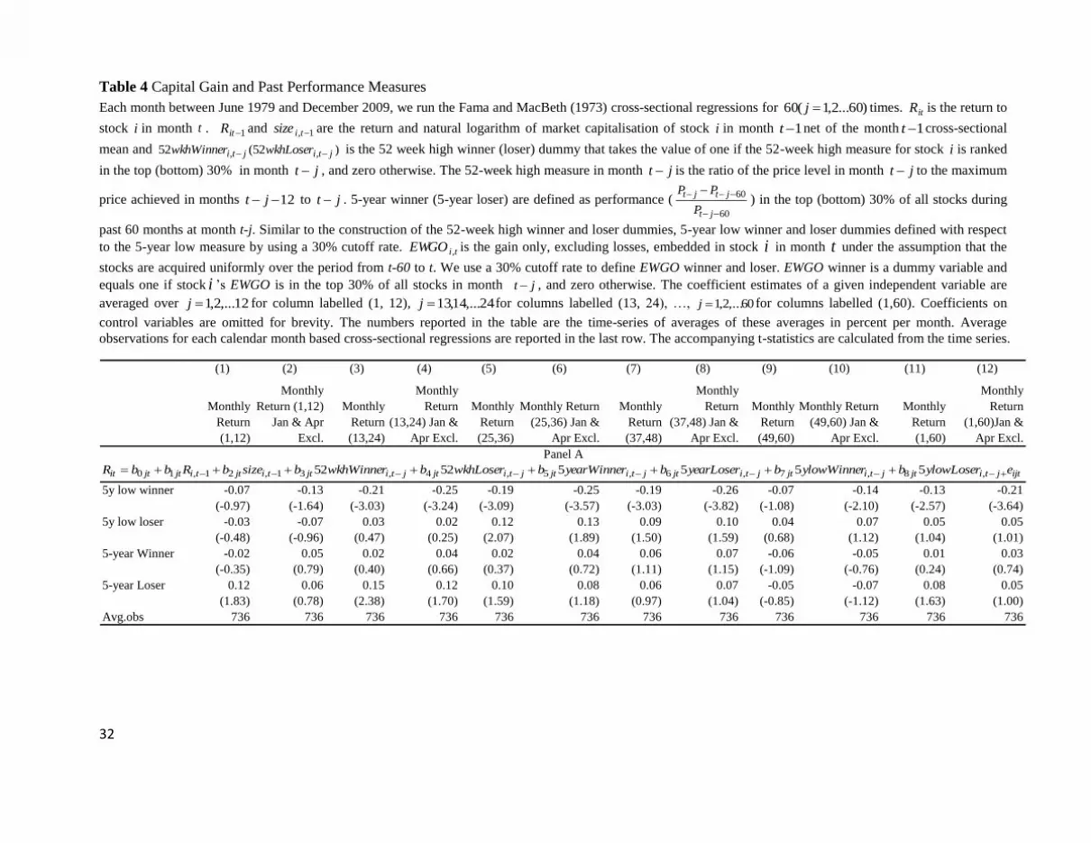
32

Table 4 Capital Gain and Past Performance Measures Each month between June 1979 and December 2009, we run the Fama and MacBeth (1973) cross-sectional regressions for )60...2,1(60 j times. itR is the return to

stock i in month t . 1itR and 1, tisize are the return and natural logarithm of market capitalisation of stock i in month 1t net of the month 1t cross-sectional

mean and )52(52 ,, jtijti wkhLoserwkhWinner is the 52 week high winner (loser) dummy that takes the value of one if the 52-week high measure for stock i is ranked

in the top (bottom) 30% in month jt , and zero otherwise. The 52-week high measure in month jt is the ratio of the price level in month jt to the maximum

price achieved in months 12 jt to jt . 5-year winner (5-year loser) are defined as performance (60

60

jt

jtjt

P

PP) in the top (bottom) 30% of all stocks during

past 60 months at month t-j. Similar to the construction of the 52-week high winner and loser dummies, 5-year low winner and loser dummies defined with respect to the 5-year low measure by using a 30% cutoff rate. tiEWGO , is the gain only, excluding losses, embedded in stock i in month t under the assumption that the

stocks are acquired uniformly over the period from t-60 to t. We use a 30% cutoff rate to define EWGO winner and loser. EWGO winner is a dummy variable and equals one if stock i ’s EWGO is in the top 30% of all stocks in month jt , and zero otherwise. The coefficient estimates of a given independent variable are averaged over 12,...2,1j for column labelled (1, 12), 24,...14,13j for columns labelled (13, 24), …, 60,...2,1j for columns labelled (1,60). Coefficients on

control variables are omitted for brevity. The numbers reported in the table are the time-series of averages of these averages in percent per month. Average observations for each calendar month based cross-sectional regressions are reported in the last row. The accompanying t-statistics are calculated from the time series.

(1) (2) (3) (4) (5) (6) (7) (8) (9) (10) (11) (12)



Jan & Apr Excl.


Monthly Return



Monthly Return (25,36) Jan &

Apr Excl.


Monthly Return



Monthly Return (49,60) Jan &

Apr Excl.


Monthly Return


5y low winner -0.07 -0.13 -0.21 -0.25 -0.19 -0.25 -0.19 -0.26 -0.07 -0.14 -0.13 -0.21(-0.97) (-1.64) (-3.03) (-3.24) (-3.09) (-3.57) (-3.03) (-3.82) (-1.08) (-2.10) (-2.57) (-3.64)

5y low loser -0.03 -0.07 0.03 0.02 0.12 0.13 0.09 0.10 0.04 0.07 0.05 0.05(-0.48) (-0.96) (0.47) (0.25) (2.07) (1.89) (1.50) (1.59) (0.68) (1.12) (1.04) (1.01)

5-year Winner -0.02 0.05 0.02 0.04 0.02 0.04 0.06 0.07 -0.06 -0.05 0.01 0.03(-0.35) (0.79) (0.40) (0.66) (0.37) (0.72) (1.11) (1.15) (-1.09) (-0.76) (0.24) (0.74)

5-year Loser 0.12 0.06 0.15 0.12 0.10 0.08 0.06 0.07 -0.05 -0.07 0.08 0.05(1.83) (0.78) (2.38) (1.70) (1.59) (1.18) (0.97) (1.04) (-0.85) (-1.12) (1.63) (1.00)

Avg.obs 736 736 736 736 736 736 736 736 736 736 736 736

Panel A

ijtjtijtjtijtjtijtjtijtjtijtjtijttijttijtjtit eylowLoserbylowWinnerbyearLoserbyearWinnerbwkhLoserbwkhWinnerbsizebRbbR ,8,7,6,5,4,31,21,10 55555252

33

Table 4 continued

EWGO winner -0.03 -0.07 -0.21 -0.26 -0.12 -0.18 -0.07 -0.15 -0.02 -0.08 -0.09 -0.15(-0.43) (-0.97) (-3.24) (-3.65) (-1.99) (-2.60) (-1.21) (-2.28) (-0.40) (-1.21) (-2.01) (-2.94)

EWGO loser 0.02 0.01 0.01 -0.01 0.14 0.14 0.13 0.13 0.06 0.08 0.07 0.07(0.26) (0.15) (0.24) (-0.09) (2.35) (2.07) (2.30) (2.05) (0.91) (1.23) (1.54) (1.36)

5-year Winner -0.05 0.01 0.04 0.04 0.02 0.02 0.02 0.01 -0.06 -0.07 0.00 0.00(-0.85) (0.20) (0.67) (0.70) (0.28) (0.32) (0.26) (0.20) (-1.06) (-1.14) (-0.16) (0.09)

5-year Loser 0.13 0.05 0.16 0.12 0.12 0.11 0.06 0.08 -0.03 -0.05 0.09 0.06(1.82) (0.69) (2.39) (1.72) (1.79) (1.44) (0.99) (1.18) (-0.57) (-0.75) (1.70) (1.13)

Avg.obs 796 796 796 796 796 796 796 796 796 796 796 796

Panel Bijtjtijtjtijtjtijtjtijtjtijtjtijttijttijtjtit eEWGOLoserbEWGOWinnerbyearLoserbyearWinnerbwkhLoserbwkhWinnerbsizebRbbR ,8,7,6,5,4,31,21,10 555252

34

Table 5 The Fama and French three-factor based Risk-Adjusted Returns for BM and 5-year Winner and Loser

Each month between June 1979 and December 2009, we run the Fama and MacBeth (1973) cross-sectional regressions for )60...2,1(60 j times.

itR is the return to stock i in month t . 1itR and 1, tisize are the return and natural logarithm of market capitalisation of stock i in month 1t net of the

month 1t cross-sectional mean and )52(52 ,, jtijti wkhLoserwkhWinner is the 52 week high winner (loser) dummy that takes the value of one if the 52-week high

measure for stock i is ranked in the top (bottom) 30% in month jt , and zero otherwise. The 52-week high measure in month jt is the ratio of the price level

in month jt to the maximum price achieved in months 12 jt to jt . 5-year winner (5-year loser) are defined as performance (60

60

jt

jtjt

P

PP) in the top

(bottom) 30% of all stocks during past 60 months at month t-j. Similar to the construction of the 52-week high winner and loser dummies, 5-year low winner and loser dummies defined with respect to the 5-year low measure by using a 30% cutoff rate. tiEWGO , is the gain only, excluding losses, embedded in stock i in

month t under the assumption that the stocks are acquired uniformly over the period from t-60 to t. We use a 30% cutoff rate to define EWGO winner and loser. For example, EWGO winner is a dummy variable and equals one if stock i ’s EWGO is in the top 30% of all stocks in month jt , and zero otherwise. To obtain risk-adjusted returns, we further run times-series of averages (one for each average), which are computed from the cross-sectional regression, on the Fama-French (1996) three-factor model. The numbers reported for risk-adjusted returns are intercepts from these time-series regressions. They are percent per month and their t-statistics are in parentheses. GRS test is the F-statistic testing the hypothesis that the intercepts in the regressions for four portfolios are jointly equal to zero. Coefficients on control variables are omitted for brevity.

(1) (2) (3) (4) (5) (6) (7) (8) (9) (10) (11) (12)


Monthly Return



Monthly Return



Monthly Return



Monthly Return



Monthly Return



Monthly Return


High BM 0.28 0.35 0.15 0.21 0.13 0.19 0.13 0.19 0.04 0.10 0.14 0.21(5.19) (5.78) (2.63) (3.46) (2.08) (3.06) (2.08) (2.82) (0.60) (1.44) (2.84) (3.81)

Low BM 0.01 0.00 0.02 0.00 0.07 0.08 0.03 0.02 0.02 0.04 0.03 0.02(0.07) (-0.02) (0.45) (-0.10) (1.21) (1.17) (0.46) (0.31) (0.29) (0.60) (0.63) (0.42)

5-year winner 0.06 0.07 -0.07 -0.06 -0.10 -0.11 -0.10 -0.08 -0.11 -0.12 -0.07 -0.08(0.60) (1.26) (-1.21) (-0.99) (-2.00) (-2.20) (-1.80) (-1.67) (-1.86) (-1.90) (-1.60) (-1.62)

5-year loser -0.14 -0.10 -0.15 -0.13 -0.02 -0.04 -0.01 -0.01 -0.10 -0.13 -0.13 -0.12(-1.62) (-1.60) (-1.85) (-1.69) (-0.30) (-0.55) (-0.24) (-0.19) (-1.49) (-1.73) (-1.54) (-1.60)

obs 366 306 366 306 366 306 366 306 366 306 366 306GRS Test 13.26 16.49 2.90 5.20 3.39 4.52 3.15 4.38 4.25 6.21 4.15 6.18p-value 0.00 0.00 0.02 0.00 0.01 0.00 0.00 0.00 0.00 0.00 0.00 0.00

ijtjtijtjtijtjtijtjtijtjtijtjtijttijttijtjtit eLBMbHBMbyearLoserbyearWinnerbwkhLoserbwkhWinnerbsizebRbbR ,8,7,6,5,4,31,21,10 555252

35

Table 6 The Fama and French three-factor based Risk-Adjusted Returns for capital gain and 5-year performance measures

Each month between June 1979 and December 2009, we run the Fama and MacBeth (1973) cross-sectional regressions for )60...2,1(60 j times. itR is the return

to stock i in month t . 1itR and 1, tisize are the return and natural logarithm of market capitalisation of stock i in month 1t net of the month 1t cross-

sectional mean and )52(52 ,, jtijti wkhLoserwkhWinner is the 52 week high winner (loser) dummy that takes the value of one if the 52-week high measure for stock

i is ranked in the top (bottom) 30% in month jt , and zero otherwise. The 52-week high measure in month jt is the ratio of the price level in month jt to

the maximum price achieved in months 12 jt to jt . 5-year winner (5-year loser) are defined as performance (60

60

jt

jtjt

P

PP) in the top (bottom) 30% of all

stocks during past 60 months at month t-j. Similar to the construction of the 52-week high winner and loser dummies, 5-year low winner and loser dummies defined with respect to the 5-year low measure by using a 30% cutoff rate. tiEWGO , is the gain only, excluding losses, embedded in stock i in month t under the

assumption that the stocks are acquired uniformly over the period from t-60 to t. We use a 30% cutoff rate to define EWGO winner and loser. For example, EWGO winner is a dummy variable and equals one if stock i ’s EWGO is in the top 30% of all stocks in month jt , and zero otherwise. To obtain risk-adjusted returns, we further run times-series of averages, which are computed from the cross-sectional regression, on the Fama-French (1996) three-factor model. The numbers reported for risk-adjusted returns are intercepts from these time-series regressions. They are percent per month and their t-statistics are in parentheses. GRS test is the F-statistic testing the hypothesis that the intercepts in the regressions for the four portfolios are jointly equal to zero. Coefficients on control variables are omitted for brevity.

36

(1) (2) (3) (4) (5) (6) (7) (8) (9) (10) (11) (12)


Monthly Return



Monthly Return



Monthly Return



Monthly Return




Jan & Apr Excl.


Monthly Return


5y low winner 0.23 0.19 0.03 0.04 -0.01 -0.05 -0.02 -0.04 0.05 0.03 0.06 0.04(3.45) (2.62) (0.56) (0.50) (-0.21) (-0.70) (-0.37) (-0.64) (0.76) (0.43) (1.24) (0.64)

5y low loser -0.22 -0.30 -0.18 -0.22 -0.11 -0.15 -0.06 -0.10 -0.09 -0.10 -0.13 -0.17(-3.20) (-3.87) (-3.20) (-3.59) (-1.95) (-2.34) (-1.00) (-1.39) (-1.42) (-1.59) (-3.24) (-3.87)

5-year Winner -0.13 -0.07 -0.05 -0.05 -0.07 -0.04 -0.06 -0.07 -0.14 -0.08 -0.09 -0.08(-2.28) (-1.14) (-0.94) (-0.77) (-1.13) (-0.51) (-0.88) (-0.96) (-2.38) (-2.70) (-2.21) (-1.79)

5-year Loser -0.05 -0.10 0.08 0.04 0.08 0.09 0.06 0.08 -0.06 -0.07 0.02 0.00(-0.67) (-1.31) (0.96) (0.55) (1.13) (1.03) (0.78) (1.02) (-0.90) (-0.94) (0.37) (0.11)

GRS Test 6.24 7.51 3.74 4.44 2.12 2.75 1.01 1.89 2.59 3.48 4.35 6.00p -value 0.00 0.00 0.01 0.01 0.07 0.03 0.39 0.11 0.04 0.01 0.01 0.00obs 366 306 366 306 366 306 366 306 366 306 366 306

EWGO winner 0.25 0.23 0.02 0.00 -0.02 -0.07 0.00 -0.02 0.05 0.04 0.06 0.04(3.87) (3.20) (0.28) (0.09) (-0.34) (-0.87) (0.03) (-0.34) (0.78) (0.59) (1.42) (0.78)

EWGO loser -0.16 -0.20 -0.17 -0.22 -0.10 -0.13 -0.06 -0.09 -0.10 -0.12 -0.12 -0.15(-2.54) (-2.89) (-3.02) (-3.49) (-1.80) (-2.15) (-0.93) (-1.43) (-1.71) (-1.86) (-2.62) (-3.10)

5-year Winner -0.14 -0.09 -0.08 -0.07 -0.10 -0.08 -0.12 -0.14 -0.20 -0.25 -0.12 -0.12(-2.37) (-1.46) (-1.15) (-0.97) (-1.54) (-1.03) (-1.87) (-1.97) (-3.13) (-3.73) (-2.81) (-2.58)

5-year Loser -0.10 -0.17 0.00 -0.04 0.03 0.01 0.00 0.00 -0.10 -0.13 -0.04 -0.07(-1.21) (-2.01) (0.00) (-0.51) (0.44) (0.18) (0.09) (0.05) (-1.53) (-1.70) (-0.58) (-0.99)

GRS Test 6.05 6.54 3.19 4.29 1.84 2.41 1.45 2.41 3.81 5.44 3.52 3.79p -value 0.00 0.00 0.02 0.00 0.12 0.05 0.21 0.05 0.01 0.00 0.01 0.01obs 366 306 366 306 366 306 366 306 366 306 366 306

Panel A

Panel B

ijtjtijtjtijtjtijtjtijtjtijtjtijttijttijtjtit eylowLoserbylowWinnerbyearLoserbyearWinnerbwkhLoserbwkhWinnerbsizebRbbR ,8,7,6,5,4,31,21,10 55555252

ijtjtijtjtijtjtijtjtijtjtijtjtijttijttijtjtit eEWGOLoserbEWGOWinnerbyearLoserbyearWinnerbwkhLoserbwkhWinnerbsizebRbbR ,8,7,6,5,4,31,21,10 555252

37

Table 7 The market and the two-factor based risk-Adjusted returns for capital gain and 5-year performance measures

Each month between June 1979 and December 2009, we run the Fama and MacBeth (1973) cross-sectional regressions for )60...2,1(60 j times. itR is the return

to stock i in month t . 1itR and 1, tisize are the return and natural logarithm of market capitalisation of stock i in month 1t net of the month 1t cross-

sectional mean and )52(52 ,, jtijti wkhLoserwkhWinner is the 52 week high winner (loser) dummy that takes the value of one if the 52-week high measure for stock

i is ranked in the top (bottom) 30% in month jt , and zero otherwise. The 52-week high measure in month jt is the ratio of the price level in month jt to

the maximum price achieved in months 12 jt to jt . 5-year winner (5-year loser) are defined as performance (60

60

jt

jtjt

P

PP) in the top (bottom) 30% of all

stocks during past 60 months at month t-j. Similar to the construction of the 52-week high winner and loser dummies, 5-year low winner and loser dummies defined with respect to the 5-year low measure by using a 30% cutoff rate. tiEWGO , is the gain only, excluding losses, embedded in stock i in month t under

the assumption that the stocks are acquired uniformly over the period from t-60 to t. We use a 30% cutoff rate to define EWGO winner and loser. For example, EWGO winner is a dummy variable and equals one if stock i ’s EWGO is in the top 30% of all stocks in month jt , and zero otherwise. To obtain risk-adjusted returns, we further run times-series of averages (one for each average), which are computed from the cross-sectional regression, on the Fama-French (1996) three-factor model ( iiifmiii eHMLhSMBsRRbaR )( ), the market model ( ifmiii eRRbaR )( ), and the two-factor model

( iifmiii eSMBsRRbaR )( ). iR is the averaged 60-month raw return in excess of risk-free rate, which we obtain from the Fama-MacBeth regressions.

mR is a market return. SMB and HML are size and value factor respectively according to the definition of Fama and French (1996). The estimates are computed

on the 60-month holding period by including all calendar months. The numbers reported for risk-adjusted returns are intercepts from these time-series regressions and their t-statistics are in parentheses. GRS test is the F-statistic testing the hypothesis that the intercepts in the regressions for four portfolios are jointly equal to zero. GRS (i), (ii) and (iii) are the tests based on the market model, the two-factor model, and the three-factor model, respectively.

38

(1) (2) (3) (4) (5) (6) (7) (8) (9) (10) (11) (12) (13)

GRS-Test

a -0.0012 -0.0012 0.0004 0.0000 -0.0000 -0.0013 -0.0002 -0.0003 -0.0009 0.0007 0.0005 0.0002(-2.43) (-2.33) (0.64) (0.04) (-0.15) (-3.24) (-0.56) (-0.70) (-2.21) (1.68) (1.38) (0.37) (i) 0.05

b 0.1828 0.2408 0.2178 -0.1777 -0.2266 -0.2098 -0.1027 -0.1329 -0.1242 0.0318 0.0490 0.0560 p-value=0.99(7.37) (9.29) (9.53) (-8.42) (-10.26) (-10.36) (-5.16) (-6.45) (-5.94) (1.30) (1.85) (2.13) (ii) 3.67

s 0.1368 0.1097 -0.1152 -0.0954 -0.0712 -0.0609 0.0406 0.0484 p-value=0.01(5.66) (5.13) (-5.59) (-5.04) (-3.58) (-3.12) (1.64) (1.96) 4.35

h -0.3687 0.2700 0.1399 0.1061 (iii) p-value=0.00(-10.42) (8.63) (4.33) (2.60)

Adj-Rsq 0.13 0.20 0.38 0.16 0.22 0.36 0.07 0.09 0.13 0.01 0.01 0.01obs 366 366 366 366 366 366 366 366 366 366 366 366

GRS-Testa -0.0009 -0.0007 0.0006 0.0003 0.0002 -0.12 -0.0004 -0.0005 -0.0012 0.0007 0.0006 -0.0003

(-1.81) (-1.73) (1.42) (0.41) (0.44) (-2.62) (-0.99) (-1.15) (-2.81) (1.64) (1.58) (-0.58) (i) 0.03b 0.1407 0.1818 0.1635 -0.1627 -0.2285 -0.2100 -0.0775 -0.1134 -0.1032 -0.0053 -0.0043 0.0090 p-value=0.99

(6.43) (7.83) (7.74) (-2.89) (-9.42) (-9.45) (-4.99) (-4.99) (-4.65) (-0.20) (-0.15) (0.30) (ii) 2.29s 0.0969 0.0754 -0.1550 -0.1333 -0.0848 -0.0727 0.0023 0.0181 p-value=0.06

(4.48) (3.82) (-6.86) (-6.41) (-4.00) (-3.51) (0.09) (0.67) 2.60h -0.2932 0.2958 0.1641 0.2143 (iii) p-value=0.03

(-8.97) (8.61) (4.78) (4.81)Adj-Rsq 0.10 0.15 0.30 0.11 0.21 0.30 0.07 0.12 0.12 0.00 0.00 0.05obs 366 366 366 366 366 366 366 366 366 366 366 366

EWGO winner EWGO loser 5-year winner 5-year loser

Panel A

5-year low winner 5-year low loser 5-year winner 5-year loser

Panel B

Long-term return reversals—Value and growth or tax? UK evidence

Documents

Transcript of Long-term return reversals—Value and growth or tax? UK evidence