Dynamic Panel Probit Models for Current Account Reversals and their Efficient Estimation

econstor www.econstor.eu

Der Open-Access-Publikationsserver der ZBW – Leibniz-Informationszentrum WirtschaftThe Open Access Publication Server of the ZBW – Leibniz Information Centre for Economics

Nutzungsbedingungen:Die ZBW räumt Ihnen als Nutzerin/Nutzer das unentgeltliche,räumlich unbeschränkte und zeitlich auf die Dauer des Schutzrechtsbeschränkte einfache Recht ein, das ausgewählte Werk im Rahmender unter→ http://www.econstor.eu/dspace/Nutzungsbedingungennachzulesenden vollständigen Nutzungsbedingungen zuvervielfältigen, mit denen die Nutzerin/der Nutzer sich durch dieerste Nutzung einverstanden erklärt.

Terms of use:The ZBW grants you, the user, the non-exclusive right to usethe selected work free of charge, territorially unrestricted andwithin the time limit of the term of the property rights accordingto the terms specified at→ http://www.econstor.eu/dspace/NutzungsbedingungenBy the first use of the selected work the user agrees anddeclares to comply with these terms of use.

zbw Leibniz-Informationszentrum WirtschaftLeibniz Information Centre for Economics

Moura, Guilherme V.; Richard, Jean-François; Liesenfeld, Roman

Working Paper

Dynamic Panel Probit Models for Current AccountReversals and their Efficient Estimation

Economics working paper / Christian-Albrechts-Universität Kiel, Department of Economics,No. 2007,11

Provided in Cooperation with:Christian-Albrechts-University of Kiel, Department of Economics

Suggested Citation: Moura, Guilherme V.; Richard, Jean-François; Liesenfeld, Roman (2007) :Dynamic Panel Probit Models for Current Account Reversals and their Efficient Estimation,Economics working paper / Christian-Albrechts-Universität Kiel, Department of Economics, No.2007,11

This Version is available at:http://hdl.handle.net/10419/22027

Dynamic Panel Probit Models for Current Account Reversals and their Efficient

Estimation

by Roman Liesenfeld, Guilherme V. Moura and Jean-François Richard

Economics Working Paper

No 2007-11

Dynamic Panel Probit Models for CurrentAccount Reversals and their Efficient Estimation

Roman Liesenfeld∗

Department of Economics, Christian Albrechts Universitat, Kiel, Germany

Guilherme V. MouraDepartment of Economics, Christian Albrechts Universitat, Kiel, Germany

Jean-Francois RichardDepartment of Economics, University of Pittsburgh, USA

May 18, 2007

Abstract

We use panel probit models with unobserved heterogeneity and se-rially correlated errors in order to analyze the determinants and thedynamics of current-account reversals for a panel of developing andemerging countries. The likelihood evaluation of these models requireshigh-dimensional integration for which we use a generic procedureknown as Efficient Importance Sampling (EIS). Our empirical resultssuggest that current account balance, terms of trades, foreign reservesand concessional debt are important determinants of the probabilityof current-account reversal. Furthermore we find under all specifi-cations evidence for serially correlated error components and weakevidence for state dependence.

JEL classification: C15; C23; C25; F32Keywords: Panel data, Dynamic discrete choice, Current account reversals, Im-portance Sampling, Monte Carlo integration, State dependence, Spillover effects.

Number of words: 9739

∗Contact author: R. Liesenfeld, Institut fur Statistik und Okonometrie, Christian-Albrechts-Universitat zu Kiel, Olshausenstraße 40-60, D-24118 Kiel, Germany; E-mail: [email protected]; Tel.: +49-(0)431-8803810; Fax: +49-(0)431-8807605.

1 Introduction

The determinants of current account reversals and their consequences for coun-

tries’ economic performance have received a lot of attention since the currency

crises of the 1990s, and have found renewed interest because of the huge current

account deficit of the US in recent years. The importance of the current account

comes from its interpretation as a restriction on countries’ expenditure abilities.

Expenditure restrictions, generated by sudden stops and/or currency crises, can

generate current account reversals, worsen an economic crises or even trigger one

(see, e.g., Milesi-Ferretti and Razin, 1996, 1998, 2000, and Obstfeld and Ro-

goff, 2004). Typical issues addressed in the recent literature are: The extent

to which current account reversals affect economic growth (Milesi-Ferretti and

Razin, 2000, and Edwards 2004a,b); The sustainability of large current account

deficits for significant periods of time (Milesi-Ferretti and Razin, 2000); and pos-

sible causes for current account reversals (Milesi-Ferretti and Razin, 1998, and

Edwards, 2004a,b). Our paper proposes to analyze the latter issue in the context

of dynamic panel probit models, paying special attention to the serial dependence

inherent to current account reversals.

Milesi-Ferretti and Razin (1998) and Edwards (2004a,b) use panel probit mod-

els in order to investigate the determinants of current account reversals. While

Milesi-Ferretti and Razin analyze a panel of low- and middle-income countries,

Edwards also includes industrialized countries. They use time and country spe-

cific dummies in order to account for heterogeneity. In addition to the fact that

it requires estimation of a large number of parameters, a fixed effect approach

raises two key issues of identification in the context of the data set we propose

to use. First, it precludes the use of potentially important explanatory variables

1

which are constant across countries or over time. Also, current account crises

are typically rare events and have not been experienced by some of the countries

included in our data set.

Following Heckman (1981a), Falcetti and Tudela (2006) argue that there are

two distinct possible sources of serial dependence which ought to be taken into

account in the context of a panel analysis of currency crisis: State dependence

and persistent heterogeneity across countries. State dependence would reflect

the possibility that past reversals could affect the probability of another reversal.

Unobserved heterogeneity would reflect differences in institutional, political or

relevant economic factors across countries which cannot be controlled for. How-

ever, as argued, e.g., by Hyslop (1999), serial dependence could also be transitory

resulting from autocorrelation, whether specific to individual countries (idiosyn-

cratic error component) or common to all (time random effect). Serial dependence

in the idiosyncratic error component may arise from a persistence of the current

account deficit itself as documented, e.g., by Edwards (2004b). Serially correlated

time random effects account for possible dynamic spillover effects of current ac-

count crises. In particular, following the financial turbulences of the 1990s, it is

recognized that spillover effects are important, especially for emerging economies.

Common causes of contagion include transmission of local shocks, such as cur-

rency crises, through trade links, competitive devaluations, and financial links

(see, e.g., Dornbusch et al., 2000).

In the present paper, we analyze the determinants and dynamics of current

account reversals for a panel of developing and emerging countries controlling

for alternative sources of persistence. Our starting point is a panel probit model

with state dependence and persistent random heterogeneity. We then analyze

the robustness of this model against the introduction of correlated idiosyncratic

2

error components (Section 3.1) or correlated common time effects (Section 3.2).

Likelihood evaluation of panel probit models with unobserved heterogeneity

and dynamic error components is complicated by the fact that the computation

of the choice probabilities requires high-dimensional interdependent integration.

The dimension of such integrals is typically given by the number of time periods

(T ), or if one allows for interaction between country specific and time random

effects by T + N , where N is the number of countries. Thus efficient likelihood

estimation of such models typically relies upon Monte-Carlo (MC) integration

techniques (see, e.g., Geweke and Keane, 2001 and the references therein). Var-

ious MC procedures have been proposed for the evaluation of such choice prob-

abilities – see, e.g., Stern (1997) for a survey. The most popular among those is

the GHK procedure which was developed by Geweke (1991), Hajivassiliou (1990),

and Keane (1994) and which has been applied to the estimation of dynamic panel

probit models, e.g., by Hyslop (1999), Greene (2004), and Falcetti and Tudela

(2006). While conceptually simple and easy to program, the GHK procedure re-

lies upon importance sampling densities which ignore critical information relative

to the underlying dynamic structure of the model. This can lead to significant de-

terioration of numerical accuracy as the dimensionality of integration increases.

In particular, Lee (1997) conducts a MC study of ML estimation under GHK

likelihood evaluation for panel models with serially correlated errors and finds

significant biases for longer panels.

In the present study we use Efficient Importance Sampling (EIS) methodology

developed by Richard and Zhang (2007), which represents a powerful and generic

high dimensional simulation technique. It is based on simple Least-Squares op-

timizations designed to maximize the numerical accuracy of the integral approx-

imations associated with the likelihood. As such, EIS is particularly well suited

3

to handle unobserved heterogeneity and serially correlated errors in panel probit

models. In particular, as illustrated below, combining EIS with GHK substan-

tially improves the numerical efficiency of the standard GHK allowing for reliable

ML estimation of dynamic panel probit models even in applications with a very

large time dimension.

In conclusion of our introduction, we note that there are a number of other

studies which empirically analyze discrete events reflecting marcoeconomic and/or

financial crises using non-linear panel models, including those of Calvo et al. (2004)

on sudden stops and those of Eichengreen et al. (1995) and Frankel and Rose

(1996) on currency crises. The study most closely related to this paper with

respect to the empirical methodology is that of Falcetti and Tudela (2006), who

analyze the determinants of currency crises using a dynamic panel probit model

accounting for different sources of intertemporal linkages among episodes of such

crises. However, contrary to our study, they do not consider specifications cap-

turing possible spillover effects of crises and their estimation strategy is based on

the standard GHK procedure.

The remainder of this paper is organized as follows. In the next section we

describe the data set and introduce the definition of a current account reversal

used in our analysis. Section 3 presents the dynamic panel probit models used to

analyze current account reversals. In Section 4 we describe the implementation

of EIS procedure in this context. Empirical results are discussed in section 5 and

some conclusions are drawn in section 6.

4

2 The Data

Our data set consists of an unbalanced panel for 60 low and middle income

countries from Africa, Asia, and Latin America and the Caribbean. The complete

list of countries is given on Table 1. The time span of the data set ranges from

1975 to 2004, although the unavailability of some explanatory variables often

restrict the analysis to smaller time dimensions. The minimum number of time

periods for a country is 9, the maximum is 18 and the average is 16.5 for a total

of 963 observations. The values of the binary dependent variable indicating the

occurrence of a current account crisis are known for the initial time period t = 0

for all countries. Therefore, the initial conditions problem for the estimation

of a dynamic discrete choice model including the lagged dependent variable, as

discussed, e.g., by Heckman (1981b), does not arise here. The sources of the

data are the World Bank’s World Development Indicators (2005) and the Global

Development Finance (2004).

Current account reversal are defined as in Milesi-Ferretti and Razin (1998).

According to this definition a current account reversal has to meet three require-

ments. The first is an average reduction of the current account deficit of at

least 3 percentage points of GDP over a period of 3 years relative to the 3-year

average before the event. The second requirement is that the maximum deficit

after the reversal must be no larger than the minimum deficit in the 3 years pre-

ceding the reversal. The last requirement is that the deficit is reduced to below

10%. The independent variables are standard in the literature and contain lagged

macroeconomic, external, debt and foreign variables that are potential indicators

of a reversal. The macroeconomic variables are the annual growth rate of GDP

(AVGGROW), the share of investment to GDP proxied by the ratio of gross cap-

5

ital formation to GDP (AVGINV), government expenditure (GOV) and interest

payments relative to GDP (INTPAY). The external variables are the current ac-

count balance as a fraction of GDP (AVGCA), a terms of trade index set equal

to 100 for the year 2000 (AVGTT), the share of exports and imports of goods

and services to GDP as a measure of trade openness (OPEN), the rate of official

transfers to GDP (OT) and the share of foreign exchange reserves to imports

(RES). The debt variables included are the share of consessional debt to total

debt and interest payments relative to the GDP (CONCDEB). Foreign variables

such as the US real interest rate (USINT) and the real growth rates of the OECD

countries (GROWOECD) are also included to reflect the influence of the world

economy. As in Milesi-Ferretti and Razin (1998), the current account, growth,

investment and terms of trade data are 3-years averages, to ensure consistency

with the way reversals are measured.

3 Empirical Specifications

The baseline specification we use for our analysis is a dynamic panel probit model

of the form

y∗it = x′itπ + κyit−1 + eit, yit = I(y∗it > 0), i = 1, ..., N, t = 1, ..., T, (1)

where I(y∗it > 0) is an indicator function that transforms the latent continuous

variable y∗it for country i in year t into the binary variable yit, indicating the

occurrence of a current account reversal. The error term eit is assumed to be

normally distributed with zero mean and a fixed variance. The vector xit contains

the observed macroeconomic, external, debt and foreign variables which might

6

affect the incidence of a reversal. The lagged dependent variable on the right hand

side is included to capture possible state dependence. It reflects the possibility

that past current account crises could lead to changes in institutional, political

or economic factors affecting the probability of another reversal.

3.1 Panel models with random country-specific effects

The most restrictive version of the panel probit assumes that the error eit is in-

dependent across time and countries and imposes the restriction κ = 0. This

produces the standard pooled probit estimator which ignores possible serial de-

pendence and unobserved heterogeneity which cannot be attributed to the vari-

ables in xit. However, countries have institutional differences such as property

rights, tax systems which are difficult to control for and which might affect their

individual propensity to experience a current account reversal. In order to take

these differences into account, fixed or random effect panel models could be used.

However, a fixed effect model based on country-specific dummy variables, such

as the one used in the studies of Milesi-Ferretti and Razin (1998) and Edwards

(2004a,b), requires the estimation of a large number of parameters, leading to

a significant loss of degrees freedom. Furthermore, since our data set includes

countries that never experienced a reversal (see Table 1), for which the depen-

dent variable does not vary, the ML-estimator does not exist. This identification

problem restricts the analysis to a random effect approach.

A prominent random effect model is that proposed by Butler and Moffitt

(1982). It assumes the following specification for the error term in Equation (1):

eit = τi + εit, εit ∼ i.i.d.N(0, 1), τi ∼ i.i.d.N(0, σ2τ ). (2)

7

The country-specific term τi captures possible permanent latent differences in the

propensity to experience a reversal. Furthermore, it is assumed that τi and εit

are independent from the variables included in xit. If, however, xit did contain

variables reflecting countries’ general susceptibility to current account crises, then

τi would be correlated with xit. Ignoring such correlation leads to inconsistent

parameter estimates. Whence, the orthogonality condition between the random

effect and the included regressors should be tested. An independence test is

discussed further below.

Notice that the time-invariant heterogeneity component τi implies a cross-

period correlation of the error term eit which is constant for all pairs of periods

and is given by corr(eit, eis) = σ2τ/(σ

2τ + 1) for t 6= s (see, e.g., Greene, 2003).

Additional potential sources of serial dependence are transitory country-specific

differences in the propensity to experience a reversal leading to serial correla-

tion in the error component εit of Equation (2). Furthermore, the intertemporal

characteristics of the current account itself (Obstfeld and Rogoff, 1996), and the

evidence of sluggish behavior of the trade balance (Baldwin and Krugman, 1989)

and of foreign direct investments (Dixit, 1992) might introduce further serial

dependence in εit. Whence, in addition to the Butler-Moffitt specification (1)

and (2), we assume here that eit includes a serially correlated idiosyncratic error

component according to

eit = τi + εit, εit = ρεit−1 + ηit, ηit ∼ i.i.d.N(0, 1), (3)

where τi and ηit are independent among each other and also from the variables

included in xit. In order to ensure stationarity we assume that |ρ| < 1.

8

3.2 Panel model with random country- and time-specific

effects

International capital markets, particularly those in emerging economies, appear

volatile and subject to spillover effects. The currency crises of the 1990s and the

way in which they rapidly spread across emerging markets including those rated as

healthy economies by analysts and multilateral institutions, have brought interest

in contagion effects (see Edwards and Rigobon, 2002). A crisis in one country may

lead investors to withdraw their investments from other markets without taking

into account differences in economic fundamentals. In addition, a crisis in one

economy can also affect the fundamentals of other countries through trade links

and currency devaluations. Trading partners of a country in which a financial

crisis has induced a sharp currency depreciation could experience a deterioration

of the trade balance resulting from a decline in exports and an increase in imports

(see Corsetti et al., 1999). These effects can lead to a deterioration of the current

account in other countries. In the words of the former Managing Director of

the IMF: “from the viewpoint of the international system, the devaluations in

Asia will lead to large current account surpluses in those countries, damaging the

competitive position of other countries and requiring them to run current account

deficit.” Fisher (1998).

Currency devaluations of countries that experience a crisis can often be seen

as a beggar-thy-neighbor policy in the sense that they incite output growth and

employment domestically at the expense of output growth, employment and cur-

rent account deficit abroad (Corsetti et al., 1999). Competitive devaluations also

happen in response to this process, as other economies may try to avoid this

competitiveness loss through a devaluation of their own currency. This appears

9

to have happened during the East Asian crises in 1997 (Dornbusch et al., 2000).

The panel probit models introduced above do not account for such spillover

effects since they ignore correlation across countries. In order to address this

issue we also consider the following factor specification for the error eit in the

probit regression (1):

eit = τi + ξt + εit, εit ∼ i.i.d.N(0, 1), (4)

with

ξt = δξt−1 + νt, νt ∼ i.i.d.N(0, σ2ξ ), (5)

where τi, εit and νt are mutually independent and independent from xit. Fur-

thermore, it is assumed that |δ| < 1. The common dynamic factor ξt represents

unobserved time-specific effects which induce correlation across countries, reflect-

ing possible spillover effects. Note that this factor specification, which was also

used in Liesenfeld and Richard (2007) for a microeconometric application, resem-

bles the linear panel models with a factor structure as discussed, e.g., in Baltagi

(2005) and primarily used for the analysis of macroeconomic data.

3.3 A note on normalization

In Equations (2) to (5), we followed the standard practice of normalizing the

probit equation (1) by setting the variance of the residual innovations equal to

1. It follows that the variances of the composite error term eit differ across

models, implying corresponding differences in the implicit normalization rule.

10

The variances of eit under the different specifications are given by

Equation (2) : σ2e = 1 + σ2

τ

Equation (3) : σ2e =

1

1− ρ2+ σ2

τ

Equations (4)+(5) : σ2e = 1 + σ2

τ +σ2

ξ

1− δ2.

These differences affect comparisons between estimated coefficients across models

(but not between estimated probabilities). The implied correction factors do not

exceed 11% for the results reported below. For the ease of comparison we shall

report the estimated standard deviation σe of eit for each model.

4 Maximum-Likelihood Estimation

ML estimation of the simple pooled panel probit model is straightforward and

essentially the same as for a single equation probit model. Efficient parameter

estimates can also be easily obtained for the Butler-Moffitt model (1) and (2). In

particular, the choice probabilities are represented by one dimensional integrals,

which can be evaluated conveniently by means of a quadrature procedure. Let

y = {{yit}Tt=1}N

i=1 and x = {{xit}Tt=1}N

i=1. Let θ denote the parameter vector to be

estimated. The likelihood function for the Butler-Moffitt random effect model is

then given by

L(θ; y, x) =N∏

i=1

{∫

R1

T∏t=1

[Φyit

it (1− Φit)(1−yit)

] 1√2πσ2

τ

exp

{−τ 2i

2σ2τ

}dτi

}, (6)

where Φit = Φ(x′itπ +κyit−1 + τi), and Φ(·) represents the cdf of the standardized

normal distribution. In the application below, the one dimensional integrals in

11

τi are evaluated using a Gauss-Hermite quadrature rule (see, e.g., Butler and

Moffitt, 1982).

Once the parameters have been estimated, the Gauss-Hermite procedure can

also be used to obtain estimates of the random country-specific effects τi. Those

estimates can serve as the basis for validating the imposed orthogonality condi-

tions between the τi’s and the included regressors. In particular, the conditional

expectation of τi given the sample information (y, x) is obtained as

τi = E(τi|y, x; θ) =

∫R τihi(yi

, τi|xi; θ)dτi∫R hi(yi

, τi|xi; θ)dτi

, (7)

where hi denotes the joint conditional pdf of yi

= {yit}Tt=1 and τi given xi =

{xit}Tt=1, as defined by the integrand of the likelihood (6). For the evaluation of

the numerator and denominator by Gauss-Hermite, the parameters θ are set to

their ML-estimates. An auxiliary regression of the estimated random effects τi

against the time average of the explanatory variables provides a direct test of the

validity of the orthogonality condition between τi and xi.

In contrast to the Butler-Moffitt model, the computation of the likelihood

for the model (1) and (3) with country-specific effects and a serially correlated

idiosyncratic error component requires the evaluation of (T+1)-dimensional inter-

dependent integrals, and that of the model (1), (4), and (5) with country-specific

and time effects the evaluation of (T +N)-dimensional integrals. Efficient estima-

tion of these models cannot be obtained by means of standard numerical integra-

tion procedures. Instead, we propose to use the EIS methodology of Richard and

Zhang (2007). EIS is a highly accurate MC integration procedure developed for

the evaluation of high-dimensional integrals and is, therefore, ideally suited for

ML estimation of non-linear panel models with unobserved random heterogeneity

12

and serially correlated errors.

In the following two subsections we provide a brief description of the EIS

implementation in the context of ML estimation of the panel probit model with

random country-specific effects and serially correlated idiosyncratic errors (sub-

section 4.1), and with random country-specific and time effects (subsection 4.2).

For the general theory of EIS, see Richard and Zhang (2007).

4.1 ML-EIS for random country-specific effects and seri-

ally correlated errors

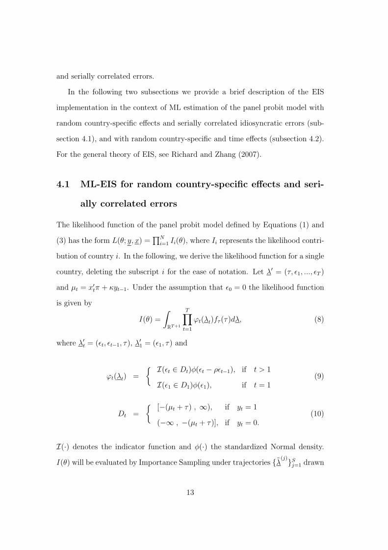
The likelihood function of the panel probit model defined by Equations (1) and

(3) has the form L(θ; y, x) =∏N

i=1 Ii(θ), where Ii represents the likelihood contri-

bution of country i. In the following, we derive the likelihood function for a single

country, deleting the subscript i for the ease of notation. Let λ′ = (τ, ε1, ..., εT )

and µt = x′tπ + κyt−1. Under the assumption that ε0 = 0 the likelihood function

is given by

I(θ) =

∫

RT+1

T∏t=1

ϕt(λt)fτ (τ)dλ, (8)

where λ′t = (εt, εt−1, τ), λ′1 = (ε1, τ) and

ϕt(λt) =

{ I(εt ∈ Dt)φ(εt − ρεt−1), if t > 1

I(ε1 ∈ D1)φ(ε1), if t = 1(9)

Dt =

{[−(µt + τ) , ∞), if yt = 1

(−∞ , −(µt + τ)], if yt = 0.(10)

I(·) denotes the indicator function and φ(·) the standardized Normal density.

I(θ) will be evaluated by Importance Sampling under trajectories {λ(j)}Sj=1 drawn

13

from an Efficient Importance Sampling density m(λ|·) constructed as described

in Richard and Zhang (2007). In order to simplify the application of sequential

EIS to the integral in (8) it proves convenient to relabel τ as λ0 and to rewrite

the integral as

I(θ) =

∫

RT+1

T∏t=0

ϕt(λt)dλ, (11)

where ϕ0(λ0) = fτ (τ). Also we partition λ′t into (εt, η′t−1

) with η′t−1

= (εt−1, λ0)

for t > 1, η0 = λ0 and η−1 = ∅. EIS aims at constructing a sequence of auxiliary

importance samplers of the form

mt(εt|ηt−1; at) =

kt(λt; at)

χt(ηt−1; at)

, t = 0, ...., T, (12)

with

χt(ηt−1; at) =

∫

Rkt(λt; at)dεt, (13)

where {kt(λt; at); at ∈ At} denote a (pre-selected) class of auxiliary paramet-

ric density kernels with χt(ηt−1; at) as analytical integrating factor in εt given

(ηt−1

, at). The integral in (11) is rewritten as

I(θ) = χ0(a0)

∫

RT+1

T∏t=0

[ϕt(λt)χt+1(ηt

; at+1)

kt(λt; at)

]mt(εt|ηt−1

; at)dλ (14)

with χT+1(·) ≡ 1. The backward transfer of the integrating factors χt+1(·) con-

stitutes the cornerstone of sequential EIS and is meant to capture as closely as

possible the dynamics of the underlying process. As discussed further below, it

is precisely the lack of such transfers which explains the inefficiency of the GHK

procedure in (large dimensional) interdependent truncated integrals. Under (14),

14

an EIS-MC estimate of I(θ) is given by

IS(θ) = χ0(a0)1

S

S∑j=1

T∏t=0

ϕt(λ(j)

t )χt+1(η(j)

t; at+1)

kt(λ(j)

t ; at)

, (15)

where {λ(j)= {λ(j)

t }Tt=0}S

j=1 denote S i.i.d. trajectories drawn from the auxiliary

sampler

m(λ|a) =T∏

t=0

mt(εt|ηt−1; at), a = (a0, ..., aT ) ∈ A = ×T

t=0At. (16)

That is to say, ε(j)t is drawn from mt(εt|η(j)

t−1; at) for t = 0, ..., T . An Efficient

Importance Sampler is one which minimizes the MC sampling variances of the

ratios ϕtχt+1/kt under such draws. Since mt(·; at) depends itself upon at, efficient

at’s obtain as solutions of the following fixed point sequences of back-recursive

auxiliary least squares (LS) problems:

(c(k+1)t , a

(k+1)t ) = arg min

ct,at

S∑j=1

{ln

[ϕt

(λ

(k,j)

t

) · χt+1

(η(k,j)

t; a

(k+1)t+1

)](17)

−ct − ln kt

(λ

(k,j)

t ; at

)}2

,

for t = T, T − 1, ..., 0, where {λ(k,j)= {λ(k,j)

t }Tt=0}S

j=1 denote trajectories drawn

from m(λ|a(k)). Convergence to a fixed point solution typically requires 3 to

5 iterations for reasonably well-behaved applications. See Richard and Zhang

(2007) for details. As starting values we propose to use those values for the

auxiliary parameters a implied by the GHK sampling densities discussed further

below.

Two additional key components of this EIS algorithm are as follows: (i) The

15

kernel kt(λt; at) has to approximate the ratio ϕt(λt) ·χt+1(ηt; at+1) with respect to

λt, not just εt in order to capture the interdependence across the εt’s. (There is no

revisiting of period t once at has been found); (ii) All trajectories {λ(k,j)}Sj=1 have

to be obtained by transformation of a single set of Common Random Numbers

(CRNs) {u(j)}Sj=1 pre-drawn from a canonical distribution, i.e. one which does not

depend on a. In the present case the CRNs consist of draws from a uniform dis-

tribution to be transformed into (truncated) gaussian draws from mt(εt|ηt−1; at)

(see Appendix 1).

Next, we discuss the specific application of EIS to the likelihood integral

defined by Equation (8). In the present section, we only present the heuristic

of such implementation. Full details are given in Appendix 1, where we show

that the EIS problem in (17) actually reduces to a univariate EIS (instead of a

trivariate one in λt) by taking full advantage of the particular structure of χt+1(·).Note first that the period-t integrand in Equation (8) includes a (truncated)

gaussian kernel. Therefore, it appears appropriate to select a gaussian kernel for

kt(λt; at), a choice further supported by the fact that we shall demonstrate that

χt(ηt; at) then takes the form of a gaussian kernel times a probability. Moreover,

the selection of a gaussian kernel enables us to take full advantage of the fact that

the class of gaussian kernels in λt is closed under multiplication (see DeGroot,

1970). Therefore, we specify kt as the following product

kt(λt; at) = ϕt(λt) · k0,t(λt; at), (18)

where k0,t is itself a gaussian kernel in λt. It immediately follows that ϕt·χt+1/kt ≡χt+1/k0,t so that ϕt cancels out in the auxiliary EIS-LS optimization problem as

defined in Equation (17). Under specification (18), we follow the standard EIS

16

implementation as described above, but need to pay attention to the fact that

λ0 = τ is present in all T + 1 factors of the integrand. Whence, we proceed as

follows:

(i) We regroup all terms in kt which only depend on λ0. Let denote the

corresponding factorization as

kt(λt; at) = k1,t(λt; at) · k3,t(λ0; at); (19)

(ii) Let χ1,t denote the integral of k1,t w.r.t. εt such that

χ1,t(ηt−1; at) =

∫

Rk1,t(λt; at)dεt. (20)

Note that this integral is truncated to Dt due to the indicator function I(εt ∈ Dt)

which is included in ϕt and, therefore, in k1,t. Since k1,t is symmetric in εt, the

(conditional) probability that εt ∈ Dt is the same as that of εt ∈ D∗t , where

D∗t = (−∞ , γt + δtλ0], with γt = (2yt − 1)µt, δt = (2yt − 1). (21)

It follows that χ1,t takes the form of a gaussian kernel in ηt−1

times the probability

that εt ∈ D∗t conditional on η

t−1, say

χ1,t(ηt−1; at) = Φ(αt + β′tηt−1

) · k2,t(ηt−1; at), (22)

where (αt, β′t) are appropriate functions of at and the data.

It follows from Equations (19) to (22) that the integral of kt w.r.t. εt is of the

form

χt(ηt−1; at) = k3,t(λ0; at)[Φ(αt + β′tηt−1

) · k2,t(ηt−1; at)]. (23)

17

In direct application of the backward transfer of integrating factors associated

with sequential EIS, the factor k3,t is transferred back directly into the period

t = 0 integral while the two factors between brackets are transferred back into

the period t− 1 integral. Full details are provided in Appendix 1.

The EIS procedure can also be used to obtain an accurate MC-estimate of

the conditional expectation of τ |y, x according to Equation (7). Under the panel

probit model (1) and (3), the joint conditional pdf of y and τ given x takes the

form

h(y, τ |x; θ) =

[∫

RT

T∏t=1

ϕt(λt)dε1 · · · dεT

]fτ (τ), (24)

which is used in Equation (7) in order to produce MC-EIS estimates of the con-

ditional expectation of τ .

We conclude this heuristic presentation of the EIS-application to the panel

probit model defined by Equations (1) and (3) with two important comments.

Firstly, as mentioned above, the MC procedure most frequently used to compute

choice probabilities is the GHK technique. It is also an importance sampling pro-

cedure but it selects ϕt itself as the auxiliary period-t kernel. The corresponding

importance sampling density is given by

mt(εt|ηt−1) =

ϕt(λt)

Φ(γt + δtλ0 + δtρεt−1), t = 1, ..., T, (25)

and m0(λ0) = fτ (τ) for period t = 0. The GHK-MC estimate of I(θ) is then

obtained as

IS(θ) =1

S

S∑j=1

[T∏

t=1

Φ(γt + δtλ(j)0 + δtρε

(j)t−1)

], (26)

where {λ(j)}Sj=1 denotes i.i.d. trajectories drawn from the sequential samplers

(m0(λ0), {mt(εt|ηt−1)}T

t=1). Note that the GHK importance sampler actually

18

belongs to the class of auxiliary EIS samplers introduced in Equation (18) since it

amounts to selecting a diffuse k0,t ∝ 1. Therefore, it is inefficient within this class.

Results of a MC experiment provided in Appendix 2 highlight the inefficiency

of GHK in the context of the particular model analyzed here. A broader MC

investigation of the relative inefficiency of GHK relative to EIS belongs to our

research agenda.

Secondly, Zhang and Lee (2004) offer a MC comparison between GHK and

AGIS, where AGIS denotes an earlier version of EIS, in the context of the same

model as that defined in Equations (1) and (3). In apparent contrast with the re-

sults presented below, they find that GHK performs essentially as well as AGIS,

except for longer panels. However, their AGIS algorithm differs from our EIS

implementation in several critical aspects. Most importantly, it ignores the fac-

torization (19) and has no direct transfer of integrating factors depending solely

on λ0 = τ . This turns out to be a major source of inefficiency since critical

information relative to τ is then filtered through the full sequence of AGIS ap-

proximations instead of being transferred directly back into the t = 0 integral.

Moreover, it would appear that AGIS optimizations are not iterated toward fixed

point solutions as in Equation (17), nor does AGIS relies upon CRNs. Last but

not least, the simulation results in Zhang and Lee are based upon i.i.d. replica-

tions of the actual sampling process (with no indications as to how the auxiliary

AGIS draws are produced across replications). Whence, the standard deviations

and/or mean squared errors they report are measures of conventional statistical

dispersions with no indications of numerical accuracy. In contrast, the results

reported below are based upon i.i.d. replications of the CRNs for a given sample

and are, therefore, meant to measure only numerical accuracy. See Richard and

Zhang (2007) for a discussion of the importance of these additional EIS refine-

19

ments.

4.2 ML-EIS for random country-specific and time effects

The likelihood function for the random effect panel model consisting of Equations

(1), (4), and (5) is given by

L(θ; y, x) =

∫

RT+N

N∏i=1

T∏t=1

[Φ(zit)]yit [1− Φ(zit)]

(1−yit)p(τ , ξ)dτ , dξ, (27)

with ξ = {ξt}Tt=1, τ = {τi}N

i=1 and zit = x′itπ + κyit−1 + τi + ξt. The presence of a

time effect ξt common to all countries prevents us from factorizing the likelihood

function into a product of integrals for each individual country. We assume

that the τi’s are independent across countries but allow for correlation among ξ.

Whence, the joint density of (τ , ξ) is assumed to be proportional to

p(τ , ξ) ∝ σ−Nτ exp

{− 1

2σ2τ

τ 2i

}|Hξ| 12 exp

{−1

2ξ′Hξξ

}, (28)

where Hξ denotes the precision matrix of ξ. See Richard (1977) for analyti-

cal expressions of Hξ under alternative initial conditions, including stationarity.

Conditionally on ξ, one could apply GHK to each country individually, though

Gauss-Hermite would likely be more efficient for these univariate integrals in

τi. One would then be left with a complicated T -dimensional integral in ξ. In

contrast, EIS can be applied to the likelihood function (27) in a way which ef-

fectively captures the complex interdependence between τ and ξ. We shall just

outline the main steps of this EIS implementation. See Richard and Zhang (2007)

or Liesenfeld and Richard (2007) for details.

20

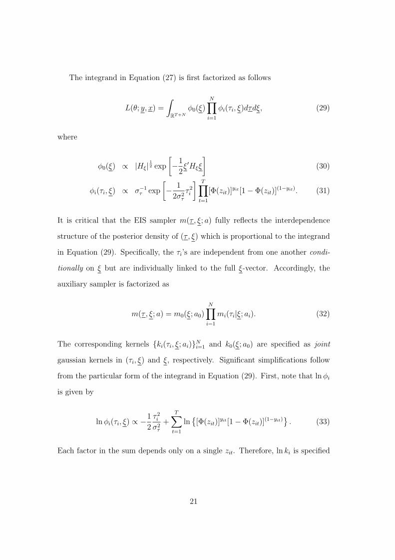
The integrand in Equation (27) is first factorized as follows

L(θ; y, x) =

∫

RT+N

φ0(ξ)N∏

i=1

φi(τi, ξ)dτdξ, (29)

where

φ0(ξ) ∝ |Hξ| 12 exp

[−1

2ξ′Hξξ

](30)

φi(τi, ξ) ∝ σ−1τ exp

[− 1

2σ2τ

τ 2i

] T∏t=1

[Φ(zit)]yit [1− Φ(zit)]

(1−yit). (31)

It is critical that the EIS sampler m(τ , ξ; a) fully reflects the interdependence

structure of the posterior density of (τ , ξ) which is proportional to the integrand

in Equation (29). Specifically, the τi’s are independent from one another condi-

tionally on ξ but are individually linked to the full ξ-vector. Accordingly, the

auxiliary sampler is factorized as

m(τ , ξ; a) = m0(ξ; a0)N∏

i=1

mi(τi|ξ; ai). (32)

The corresponding kernels {ki(τi, ξ; ai)}Ni=1 and k0(ξ; a0) are specified as joint

gaussian kernels in (τi, ξ) and ξ, respectively. Significant simplifications follow

from the particular form of the integrand in Equation (29). First, note that ln φi

is given by

ln φi(τi, ξ) ∝ −1

2

τ 2i

σ2τ

+T∑

t=1

ln{[Φ(zit)]

yit [1− Φ(zit)](1−yit)

}. (33)

Each factor in the sum depends only on a single zit. Therefore, ln ki is specified

21

as follows

ln ki(τi, ξ; ai) = −1

2

[τ 2i

σ2τ

+T∑

t=1

(αi,tz2i,t + 2βi,tzi,t)

](34)

for a total of 2 · T auxiliary parameters plus the intercept. It follows that, at the

cost of standard algebraic operations χi(ξ; ai) (i.e. the integrating constant for

ki) is itself a gaussian kernel in ξ. Whence, the product φ0(ξ) ·∏N

i=1 χi(ξ; ai) is

a gaussian kernel and requires no further adjustment (an interesting example of

perfect fit in an EIS auxiliary regression).

Estimates for the unobserved random effects are obtained, in the same way

as under the panel model without time effects, as by-products of the ML-EIS

parameter estimates. In particular, the conditional expectation of the vector of

random effects υ = (τ , ξ) given the sample information has the form

υ = E(υ|y, x; θ) =

∫RN+T υ h(y, υ|x; θ)dυ∫RN+T h(y, υ|x; θ)dυ

, (35)

where h denotes the joint conditional pdf of y and υ given x which is given by

the integrand of the likelihood function (27).

5 Empirical Results

The ML estimate of the pooled probit model (1) under the assumption that the

errors are independent across time and countries are presented in Table 2. The

results for the static model (κ = 0) are reported in the left columns and those of

the dynamic specification including the lagged dependent in the right columns.

The parameter estimates are all in line with the results in the empirical litera-

ture on current account crises (see Milesi-Ferretti and Razin, 1998, and Edwards

2004a,b). Sharp reductions of the current-account deficit are more likely in coun-

22

tries with a high current account deficits (AVGCA) and with higher government

expenditures (GOV). The significant effect of the current account deficit level is

consistent with a need for sharp corrections in the trade balance to ensure that the

country remains solvent. Interpreting current account as a constraint on expendi-

tures, the positive impact of government expenditure on the reversal probability

can be attributed to fact that an increase of government expenditures leads to a

deterioration of the current account. However, the inclusion of the lagged depen-

dent variable reduces this effect and makes it non significant. This suggests that

government expenditures might capture some omitted serial dependence under

the static specification. The coefficient of foreign reserve (RES) is negative and

significant which suggests that low levels of reserves make it more difficult to sus-

tain a large trade imbalance and may also reduce foreign investors’ willingness to

lend (Milesi-Ferretti and Razin, 1998). Also, reversals seem to be less common

in countries with a high share of concessional debt (CONCDEB). This would

be consistent with the fact that concessional debts tend to be higher in coun-

tries which have difficulties reducing external imbalances. Finally, countries with

weaker terms of trade (AVGTT) and higher GDP growth (AVGGROW) seem

to face higher probabilities of reversals, especially when growth rate in OECD

countries (GROWOECD) and/or US interest rate (USINT) are higher – though

none of these four coefficients are statistically significant.

The inclusion of the lagged current account reversal variable substantially

improves the fit of the model as indicated by the highly significant increase of

the maximized log-likelihood value. The estimated coefficient κ measuring the

impact of the lagged dependent state variable is positive and significant at the

1% significance level. This suggests that a current account reversal significantly

increases the probability of a further reversal the following year.

23

Table 3 reports the estimates of the Butler-Moffitt model (1) and (2), which

includes random country specific effects, leading to equicorrelated errors across

time periods. The ML-estimates are obtained using a 20-points Gauss Hermite

quadrature. The estimate of the coefficient στ indicates that only 3% of the total

variation in the latent error is due to unobserved country-specific heterogene-

ity and this effect is not statistically significant. Nevertheless, the maximized

log-likelihood of the Butler-Moffitt model is significantly larger than that of the

dynamic pooled probit model with a likelihood-ratio (LR) test statistic of 5.57.

Since the parameter value under the Null hypothesis στ = 0 lies at the bound-

ary of the admissible parameter space, the distribution of the LR-statistic under

the Null is a (0.5χ2(0) + 0.5χ2

(1))-distribution, where χ2(0) represents a degenerate

distribution with all its mass at origin (see, e.g., Harvey, 1989). Whence, the crit-

ical value for a significance level of 1% is the 0.98-quantile of a χ2(1)-distribution

which equals 5.41. All in all, this evidence in favor of the random effect specifica-

tion is not overwhelming. Actually, the coefficients of the explanatory variables

and of the lagged dependent state are similar (after adjusting for the different

normalization rules) under both specifications.

The estimated probit model with random effects assumes that τi is indepen-

dent of xit. If this were not correct, the parameter estimates would be inconsis-

tent. In order to check this assumption we ran the following auxiliary regression:

τi = ψ0 + x′i·ψ1 + ζi, i = 1, ..., n, (36)

where the vector xi· contains the mean values of the xit-variables (except for the

US interest rate and the OECD growth rate) over time. The value of the F -

statistic for the null ψ1 = 0 is 1.85 with critical values of 2.03 and 1.73 for the 5%

24

and 10% significance levels. Whence, evidence that τi might be correlated with

xi· is inconclusive.

We now turn to the ML estimates of the dynamic random effect model with

serially correlated idiosyncratic errors as specified by Equations (1) and (3). This

allows for a third source of serial dependence in addition to state dependence and

time-invariant unobserved heterogeneity. The ML-EIS estimation results based

on S = 100 EIS draws and three EIS (fixed-point) iterations are given in the

left columns of Table 4. The MC (numerical) standard deviations are computed

from 20 ML-EIS estimations under i.i.d. sets of CRNs. They are much smaller

than the corresponding asymptotic (statistical) standard deviations indicating

that the ML-EIS results are numerically very accurate.

The estimation results indicate that the inclusion of a transitory idiosyncratic

error component has significant effects on the dynamic structure of the model

but not on the other coefficients which remain quantitatively close to those of

the Butler-Moffitt specification. The persistence parameter estimate of ρ equal

0.4 and is statistically significant at the 1% level. Furthermore, the estimated

coefficient κ associated with the lagged dependent variable is now substantially

smaller and not significantly different from zero. This suggests that the state de-

pendence found under the pooled probit and the Butler-Moffitt model is spurious

and the result of an improper dynamic specification of the error term (see Heck-

man 1981a). Since the parameter στ governing the time-invariant heterogeneity

is also not statistically significant, the only source of serial dependence which is

relevant for current account crises appears to be the transitory country-specific

differences. Note that while the coefficient of ρ is significant at the 1% level,

the corresponding LR-statistic equals 2.57 and is not significant. Such discrep-

ancy suggests that the lagged dependent variable in the Butler-Moffitt model acts

25

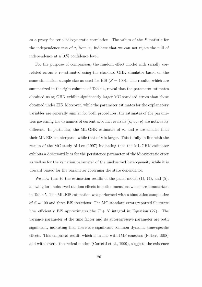
as a proxy for serial idiosyncratic correlation. The values of the F -statistic for

the independence test of τi from xi· indicate that we can not reject the null of

independence at a 10% confidence level.

For the purpose of comparison, the random effect model with serially cor-

related errors is re-estimated using the standard GHK simulator based on the

same simulation sample size as used for EIS (S = 100). The results, which are

summarized in the right columns of Table 4, reveal that the parameter estimates

obtained using GHK exhibit significantly larger MC standard errors than those

obtained under EIS. Moreover, while the parameter estimates for the explanatory

variables are generally similar for both procedures, the estimates of the parame-

ters governing the dynamics of current account reversals (κ, στ , ρ) are noticeably

different. In particular, the ML-GHK estimates of στ and ρ are smaller than

their ML-EIS counterparts, while that of κ is larger. This is fully in line with the

results of the MC study of Lee (1997) indicating that the ML-GHK estimator

exhibits a downward bias for the persistence parameter of the idiosyncratic error

as well as for the variation parameter of the unobserved heterogeneity while it is

upward biased for the parameter governing the state dependence.

We now turn to the estimation results of the panel model (1), (4), and (5),

allowing for unobserved random effects in both dimensions which are summarized

in Table 5. The ML-EIS estimation was performed with a simulation sample size

of S = 100 and three EIS iterations. The MC standard errors reported illustrate

how efficiently EIS approximates the T + N integral in Equation (27). The

variance parameter of the time factor and its autoregressive parameter are both

significant, indicating that there are significant common dynamic time-specific

effects. This empirical result, which is in line with IMF concerns (Fisher, 1998)

and with several theoretical models (Corsetti et al., 1999), suggests the existence

26

of contagion effects among developing countries. The values of the F -statistic for

the independence test indicate that there is no evidence for correlation, neither

between the time effects ξt and x·t, where x·t contains the mean values of the

explanatory variables across countries, nor between the country effects τi and xi·

(see Equation 36).

Furthermore, note that the state-dependence coefficient κ is statistically sig-

nificant, while the country-specific random effect is again not significantly dif-

ferent from zero. Hence, under the model with time-specific effects the lagged

dependent variable seems to act (similar as under the Butler-Moffitt model) as a

proxy for positive serial idiosyncratic correlation. Notice that the serial correla-

tion associated with the factor ξt is negative and is common to all countries. A

comparison between the model with serially correlated idiosyncratic errors (Table

4) and that allowing random effects in both dimensions (Table 5) reveals that

both are virtually observationally equivalent with very similar coefficients for all

explanatory variables in xit.

All in all, we find under all dynamic panel models significant serial correlation

characterizing the dynamics of current account crises. Furthermore, there is no

evidence for persistent unobserved heterogeneity across country as a possible

source for serial dependence. Finally, the data do not allow to discriminate

cleary between serially correlated idiosyncratic errors, state dependence and/or

dynamic spill over effects as potential sources of serial dependence.

6 Conclusion

This paper uses different non-linear panel data specifications to investigate the

causes and dynamics of current account reversals in low- and middle-income

27

countries. In particular, we analyze four sources of serial persistence: a country-

specific random effect, a serially correlated transitory error component, dynamic

spill over effects, and a state dependence component to control for the effect of

previous events of current account reversal.

For likelihood-based estimation of panel models with country-specific ran-

dom heterogeneity and serially correlated error components we propose to use

Efficient Importance Sampling (EIS) which represents a Monte Carlo (MC) in-

tegration technique. The application of EIS allows for numerically very accurate

and reliable ML estimation of those models. In particular, it improves signifi-

cantly the numerical efficiency of GHK, which is the most frequently used MC

procedure to estimate non-linear panel models with serially correlated errors.

Our empirical results show that the static pooled probit model is unable to

capture the dynamic patterns of the data and that the inclusion of the lagged de-

pendent variable significantly increases the fit of the model. In turn, that variable

appears to be only a proxy for an autoregressive error structure capturing transi-

tory unobserved differences across countries. ML-EIS estimation of a panel probit

with unobserved individual heterogeneity and autocorrelated idiosyncratic errors

finds that the autocorrelation coefficient of the error term is statistically signif-

icant, while both the lagged dependent and the country-specific random effect

are not. Finally, the ML-EIS estimate of a panel probit model with unobserved

individual heterogeneity, as well as a correlated time-specific effects reveals that

the time-specific effects indicative of contagion effects among developing countries

are siginificant. We found, however, that the model with unobserved individual

heterogeneity and serially correlated idiosyncratic errors and that with random

country-specific and correlated time-effects are virtually observationally equiva-

lent with very similar coefficients for all explanatory variables.

28

The empirical results of both models suggest that countries with high current

account imbalances, low foreign reserves, a small fraction of concessional debt,

and unfavorable terms of trades are more likely to experience a current account

reversal.

Acknowledgement

Roman Liesenfeld and Guilherme V. Moura acknowledge research support pro-

vided by the Deutsche Forschungsgemeinschaft (DFG) under grant HE 2188/1-1;

Jean-Francois Richard acknowledges the research support provided by the Na-

tional Science Foundation (NSF) under grant SES-0516642.

Appendix 1: EIS-implementation for random country-

specific effects and serially correlated errors

This appendix details the implementation of the EIS procedure for the panel

probit model (1) and (3) to obtain MC estimates for the likelihood contribution

I(θ) given by equation (8). In order to take full advantage of the properties of

gaussian kernels, we adopt the following conventions:

(i) Gaussian kernels are represented under their natural parametrization – see

Lehmann (1986, section 2.7). Whence, kt(λt; at) in Equation (19) is parameter-

ized as

kt(λt; at) =I(εt ∈ D∗

t )√2π

exp

{−1

2(λ′tPtλt + 2λ′tqt)

}, (A-1)

with D∗t = (−∞ , γt + δtλ0]. The EIS parameter at consists of the six lower

29

diagonal elements of Pt and the three elements in qt (the positivity constraint on

Pt never binds in our application).

(ii) All factorizations of kt are based upon the Cholesky decomposition of Pt

into

Pt = Lt∆tL′t, (A-2)

where Lt = {lij,t} is a lower triangular matrix with ones on the diagonal and ∆t

is diagonal matrix with diagonal elements di,t ≥ 0. Let

l1,t = (l21,t, l31,t)′, l2,t = (1, l32,t)

′. (A-3)

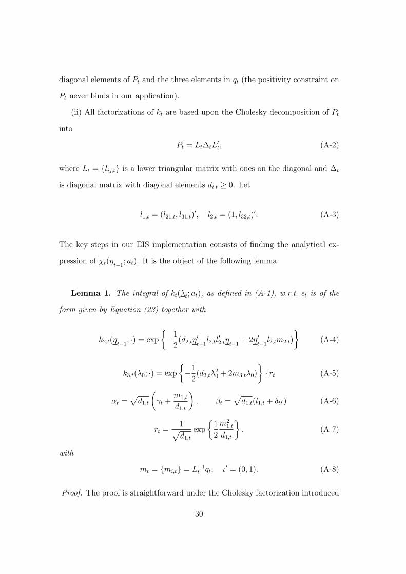
The key steps in our EIS implementation consists of finding the analytical ex-

pression of χt(ηt−1; at). It is the object of the following lemma.

Lemma 1. The integral of kt(λt; at), as defined in (A-1), w.r.t. εt is of the

form given by Equation (23) together with

k2,t(ηt−1; ·) = exp

{−1

2(d2,tη

′t−1

l2,tl′2,tηt−1

+ 2η′t−1

l2,tm2,t)

}(A-4)

k3,t(λ0; ·) = exp

{−1

2(d3,tλ

20 + 2m3,tλ0)

}· rt (A-5)

αt =√

d1,t

(γt +

m1,t

d1,t

), βt =

√d1,t(l1,t + δtι) (A-6)

rt =1√d1,t

exp

{1

2

m21,t

d1,t

}, (A-7)

with

mt = {mi,t} = L−1t qt, ι′ = (0, 1). (A-8)

Proof. The proof is straightforward under the Cholesky factorization introduced

30

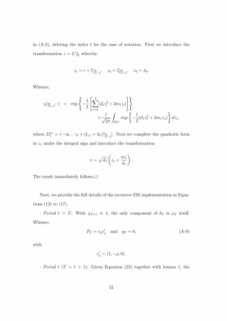
in (A-2), deleting the index t for the ease of notation. First we introduce the

transformation z = L′λ, whereby

z1 = ε + l′1η−1, z2 = l′2η−1

, z3 = λ0.

Whence,

χ(η−1; ·) = exp

{−1

2

[3∑

i=2

(diz2i + 2mizi)

]}

× 1√2π

∫

D∗∗t

exp

{−1

2(d1z

21 + 2m1z1)

}dz1,

where D∗∗t = (−∞ , γt + (l1,t + δtι)

′η−1]. Next,we complete the quadratic form

in z1 under the integral sign and introduce the transformation

v =√

d1

(z1 +

m1

d1

).

The result immediately follows.2

Next, we provide the full details of the recursive EIS implementation in Equa-

tions (12) to (17).

· Period t = T : With χT+1 ≡ 1, the only component of kT is ϕT itself.

Whence,

PT = eρe′ρ and qT = 0, (A-9)

with

e′ρ = (1,−ρ, 0).

· Period t (T > t > 1): Given Equation (23) together with lemma 1, the

31

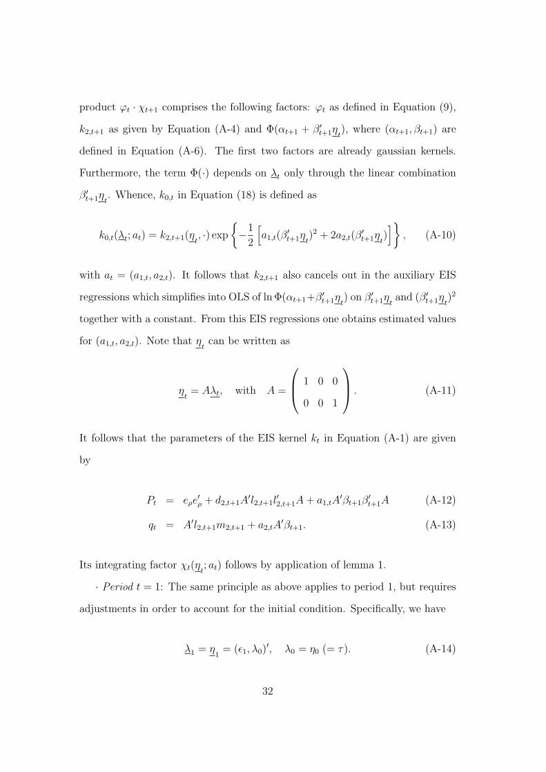
product ϕt · χt+1 comprises the following factors: ϕt as defined in Equation (9),

k2,t+1 as given by Equation (A-4) and Φ(αt+1 + β′t+1ηt), where (αt+1, βt+1) are

defined in Equation (A-6). The first two factors are already gaussian kernels.

Furthermore, the term Φ(·) depends on λt only through the linear combination

β′t+1ηt. Whence, k0,t in Equation (18) is defined as

k0,t(λt; at) = k2,t+1(ηt, ·) exp

{−1

2

[a1,t(β

′t+1ηt

)2 + 2a2,t(β′t+1ηt

)]}

, (A-10)

with at = (a1,t, a2,t). It follows that k2,t+1 also cancels out in the auxiliary EIS

regressions which simplifies into OLS of ln Φ(αt+1+β′t+1ηt) on β′t+1ηt

and (β′t+1ηt)2

together with a constant. From this EIS regressions one obtains estimated values

for (a1,t, a2,t). Note that ηtcan be written as

ηt= Aλt, with A =

1 0 0

0 0 1

. (A-11)

It follows that the parameters of the EIS kernel kt in Equation (A-1) are given

by

Pt = eρe′ρ + d2,t+1A

′l2,t+1l′2,t+1A + a1,tA

′βt+1β′t+1A (A-12)

qt = A′l2,t+1m2,t+1 + a2,tA′βt+1. (A-13)

Its integrating factor χt(ηt; at) follows by application of lemma 1.

· Period t = 1: The same principle as above applies to period 1, but requires

adjustments in order to account for the initial condition. Specifically, we have

λ1 = η1

= (ε1, λ0)′, λ0 = η0 (= τ). (A-14)

32

This amounts to replacing A by I2 in Equations (A-11) to (A-13). Whence, the

kernel k1(λ1, a1) needs only be bivariate with

P1 = e1e′1 + d2,2l2,2l

′2,2 + a1,1β2β

′2 (A-15)

q1 = l2,2m2,2 + a2,1β2, (A-16)

with e′1 = (1, 0). Essentially, P1 and q1 have lost their middle row and/or column.

To avoid changing notation in lemma 1, the Cholesky decomposition of P1 is

parameterized as

L1 =

1 0

l31,1 1

, D1 =

d1,1 0

0 d3,1

, l1,1 = l31,1, (A-17)

while d2,2 and l2,2 are now zero. Under these adjustments in notation, lemma 1

still applies with k2(η0; ·) ≡ 1 and β1 reduced to the scalar

β1 =√

d1,1(l1,1 + δ1). (A-18)

· Period t = 0 (untruncated integral w.r.t. λ0 ≡ τ): Accounting for the back

transfer of {k3,t(λ0; ·)}Tt=1, all of which are gaussian kernels, the λ0-kernel is given

by

k0(λ0; ·) = fτ (λ0) ·T∏

t=1

k3,t(λ0; ·) · exp

{−1

2

(a1,0λ

20 + 2a2,0λ0

)}, (A-19)

where (a1,0, a2,0) are the (fixed point) coefficients of the EIS approximation of

ln Φ(α1 + β1λ0). Note that k0 is the product of T + 2 gaussian kernels in λ0 and

is, therefore, itself a gaussian kernel, whose mean m0 and variance v20 trivially

33

obtain by addition from Equation (A-19).

As mentioned above, fixed point convergence of the EIS auxiliary regressions

(17) as well as continuity of corresponding likelihood estimates require the use

of CRNs. In order to draw the εt’s from their (truncated) gaussian samplers

mt(εt|ηt−1; at) based on CRNs one can use the following result: If ε follows a

truncated N(µ, σ2) distribution with bl < ε < bu, then a ε-draw is obtained as

(see, e.g., Train, 2003)

ε = µ + σΦ−1

[Φ

(bl − µ

σ

)+ u ·

{Φ

(bu − µ

σ

)− Φ

(bl − µ

σ

)}], (A-20)

where u is a canonical draw from the U(0, 1) distribution which is independent

from the parameters indexing the distribution of ε.

Appendix 2: MC experiments on the numerical

efficiency of EIS

In order to compare the numerical accuracy of EIS relative to GHK, we evaluated

the integral in Equation (8) under 18 artificial data sets considering three different

values of ρ (0.2, 0.5, 0.9), two different values of στ (0.1, 0.5) and three different

sample sizes (T=10, 20, 50). All other coefficients are set equal to zero.

For each of these eighteen data sets, we produced 200 i.i.d MC estimates of Ii

based upon different sets of CRNs. Both GHK and EIS individual estimates are

based upon S = 200 auxiliary draws and the number of EIS iterations is fixed at

three. In Table A1 we report the means, MC standard deviations and coefficients

of variation of the 200 replications under both methods for the eighteen scenarios.

As discussed in Richard and Zhang (2007), these standard deviations provide

34

direct measures of numerical accuracy. Note immediately that the MC standard

deviation under EIS are systematically lower than those under GHK, by factors

ranging from 7 to 315.

As expected numerical accuracy is a decreasing function of ρ, στ and T . This

is especially the case for GHK with coefficient of variations above 1 for T = 50

and ρ = 0.9. In sharp contrast, the worse case scenario for EIS (T = 50, ρ = 0.9,

στ = 0.5) has a coefficient of variation of 0.017. A more extensive and detailed

MC comparison of GHK and EIS belongs to our research agenda.

35

References

Baldwin, R., Krugman, P., 1989. Persistent trade effects of large exchange rate

schocks. The Quaterly Journal of Economics 54, 635–654.

Baltagi, B., 2005. Econometric Analysis of Panel Data. John Wiley & Sons.

Butler, J.S., Moffitt, R., 1982. A computationally efficient quadrature procedure for

the one-factor multinomial probit model. Econometrica 50, 761–764.

Calvo, G., Izquierdo, A., Mejia, L.F., 2004. On the empirics of sudden stops: the

relevance of balance-sheet effects. Working paper. Inter-American Development

Bank.

Corsetti, G., Pesenti, P., Roubini, N., Tille, C. 1999. Competitive devaluations: a

welfare-based approach. NBER-Working Paper No 6889.

DeGroot, M.H., 1970. Optimal Statistical Decisions. McGraw-Hill.

Devroye, L., 1986. Non-Uniform Random Variate Generation. Springer-Verlag.

Dixit, A., 1992. Investment and Hysteresis. The Journal of Economic Perspectives 6,

107–132.

Dornbusch, R., Park, Y.C., Claessens, S., 2000. Contagion: Understanding how it

spreads. World Bank Research Observer 15, 177–197.

Edwards, S., 2004a. Financial openness, sudden stops and current account reversals.

American Economic Review 2, 59-64.

Edwards, S., 2004b. Thirty years of current account imbalances, current account

reversals, and sudden stops. NBER-Working Paper No. 10276.

Edwards, S., Rigobon, R. 2002. Currency crises and contagion: an introduction.

Journal of Development Economics 69, 307–313.

36

Eichengreen, B., Rose, A., Wyplosz 1995. Exchange rate mayhem: the antecedents

and aftermath of speculative attacks. Economic Policy 21, 249–312.

Falcetti, E., Tudela, M., 2006. Modelling currency crises in emerging markets: a

dynamic probit model with unobserved heterogeneity and autocorrelated errors.

Oxford Bulletin of Economics and Statistics 68, 445–471.

Fisher, S., 1998. The IMF and the asian crisis. Los Angeles, March 20.

Frankel, J., Rose, A., 1996. Currency crashes in emerging markets: an empirical treat-

ment. Board of Governors of the Federal Reserve System Oxford, International

Finance Diskussion Papers 534, 1–28.

Geweke, J., 1991. Efficient simulation from the multivariate normal and student-

t distributions subject to linear constraints. Computer Science and Statistics:

Proceedings of the Twenty-Third Symposium on the Interface, 571–578.

Geweke, J., Keane, M., 2001. Computationally intensive methods for integration

in econometrics. In Heckman, J., Leamer, E., Handbook of Econometrics 5,

Chapter 56. Elsevier.

Greene, W., 2003. Econometrics Analysis. Prentice Hall, Englewood Cliffs.

Greene, W., 2004. Convenient estimators for the panel probit model: further results.

Empirical Economics 29, 21–47.

Hajivassiliou, V., 1990. Smooth simulation estimation of panel data LDV models.

Mimeo. Yale University.

Harvey, A., 1989. Forecasting, Structural Time Series Models and Kalman Filter.

Cambridge University Press.

Heckman, J., 1981a. Statistical models for discrete panel data. In Manski, C.F., Mc-

Fadden, D., Structural Analysis of Discrete Data with Econometric Applications.

37

The MIT Press.

Heckman, J., 1981b. The incidental parameter problem and the problem of initial con-

ditions in estimating a discrete time-discrete data stochastic process. In Manski,

C.F., McFadden, D., Structural Analysis of Discrete Data with Econometric Ap-

plications. The MIT Press.

Hyslop, D., 1999. State Dependence, serial correlation and heterogeneity in intertem-

poral labor force participation of married women. Econometrica 67, 1255–1294.

Keane, M., 1994. A computationally practical simulation estimator for panel data.

Econometrica 62, 95–116.

Lee, L-F., 1997. Simulated maximun likelihood estimation of dynamic discrete choice

models – some Monte Carlo results. Journal of Econometrics 82, 1–35.

Lehmann, E.L., 1986. Testing Statistical Hypotheses. John Wiley & Sons.

Liesenfeld, R., Richard, J.F., 2007. Simulation techniques for panels: Efficient impor-

tance sampling. manuscript, University of Kiel , Dept. of Economics. (to appear

in: Matyas, L., Sevestre, P., The Economterics of Panel Data (3rd ed). Kluwer

Academic Publishers.)

Milesi-Ferretti, G.M., Razin, A., 1996. Current account sustainability: Selected east

asian and latin american experiences. NBER-Working Paper No. 5791.

Milesi-Ferretti, G.M., Razin, A., 1998. Sharp reductions in current account deficits:

An empirical analysis. European Economic Review 42, 897–908.

Milesi-Ferretti, G.M., Razin, A., 2000. Current account reversals and currency crisis:

empirical regularities. In Krugman, P., Currency Crises. University of Chicago

Press.

38

Obstfeld, M., Rogoff, K. 1996. Foundations of International Macroeconomics. The

MIT Press.

Obstfeld, M., Rogoff, K., 2004. The unsustainable US current account position revis-

ited. NBER-Working paper No. 10869.

Richard, J.-F., 1977. Bayesian analysis of the regression model when the disturbances

are generated by an autoregressive process. In Aykac, A., Brumat, C., New de-

velopments in the application of Bayesian methods. North Holland, Amsterdam.

Richard, J.-F., Zhang, W., 2007. Efficient high-dimensional importance sampling.

Forthcoming in: Journal of Econometrics.

Stern, S., 1997. Simulation-based estimation. Journal of Economic Literature 35,

2006–2039.

Train, K.E., 2003. Discrete Choice Methods with Simulation. Cambridge University

Press.

Zhang, W., Lee, L.-F., 2004. Simulation estimation of dynamic discrete choice panel

models with accelerated importance samplers. Econometrics Journal 7, 120–142.

39

Tab

le1.

Lis

tof

countr

ies

Cou

ntr

yIn

itia

lO

bs.

Fin

alO

bs.

Rev

ersa

lsA

rgen

tina

1988

2001

2B

angl

ades

h19

8420

000

Ben

in19

8419

992

Bol

ivia

1984

2001

3B

otsw

ana

1984

2000

2B

razi

l19

8420

011

Burk

ina

Fas

o19

8419

920

Buru

ndi

1989

2001

0C

amer

oon

1984

1993

0C

entr

alA

fric

anR

epublic

1984

1992

0C

hile

1984

2001

3C

hin

a19

8620

011

Col

ombia

1984

2001

4C

ongo

Rep

.19

8420

012

Cos

taR

ica

1984

2001

1C

ote

d’Ivo

ire

1984

2001

5D

omin

ican

Rep

ublic

1984

2001

2E

cuad

or19

8420

011

Egy

pt

1984

2001

3E

lSal

vador

1984

2001

2G

abon

1984

1997

3G

ambia

1984

1995

1G

han

a19

8420

011

Guat

emal

a19

8420

010

Guin

ea-B

issa

u19

8719

950

Hai

ti19

8419

983

Hon

dura

s19

8420

012

Hunga

ry19

8620

011

India

1984

2001

0In

don

esia

1985

2001

1

Cou

ntr

yIn

itia

lO

bs.

Fin

alO

bs.

Rev

ersa

lsJor

dan

1984

2001

4K

enya

1984

2001

2Les

otho

1984

2000

0M

adag

asca

r19

8420

010

Mal

awi

1984

2001

0M

alay

sia

1984

2001

5M

ali

1991

2000

0M

auri

tania

1984

1996

4M

exic

o19

8420

011

Mor

occ

o19

8420

012

Nig

er19

8419

931

Nig

eria

1984

1997

2Pak

ista

n19

8420

013

Pan

ama

1984

2001

2Par

aguay

1984

2001

2Per

u19

8420

012

Philip

pin

es19

8420

013

Rw

anda

1984

2001

1Sen

egal

1984

2001

3Sey

chel

les

1989

2001

4Sie

rra

Leo

ne

1984

1995

0Sri

Lan

ka19

8419

972

Sw

azilan

d19

8420

013

Thai

land

1984

2001

3Tog

o19

8420

000

Tunis

ia19

8420

012

Turk

ey19

8420

010

Uru

guay

1984

2001

0V

enez

uel

a19

8420

011

Zim

bab

we

1984

1992

2

40

Table 2. ML-estimates of the pooled probit model

Static Model Dynamic Model

Variable Estimate Asy. s.e. Estimate Asy. s.e.Constant −1.993∗∗∗ 0.474 −1.955∗∗∗ 0.493AVGCA −0.060∗∗∗ 0.012 −0.060∗∗∗ 0.012AVGGROW 0.008 0.021 0.009 0.021AVGINV −0.002 0.010 0.001 0.011AVGTT −0.108 0.066 −0.109 0.069GOV 0.026∗∗ 0.012 0.018 0.012OT −0.011 0.010 −0.011 0.010OPEN −0.058 0.087 −0.085 0.090USINT 0.108 0.073 0.107 0.075GROWOECD 0.084 0.086 0.042 0.090INTPAY 0.024 0.029 0.021 0.030RES −0.074∗∗ 0.030 −0.074∗∗ 0.030CONCDEB −0.165∗∗ 0.068 −0.152∗∗ 0.071κ 0.981∗∗∗ 0.158

Log-likelihood −276.13 −257.26

Note: The estimated model is given by Equation (1) assuming thatthe errors are independent across countries and time. The asymp-totic standard errors are calculated as the square root of the diagonalelements of the inverse Hessian. ∗,∗∗, and ∗∗∗ indicates statistical sig-nificance at the 10%, 5% and 1% significance level.

41

Table 3. ML-estimates of the dynamic Butler-Moffittrandom effect model

Variable Estimate Asy. s.e.Constant −1.880∗∗∗ 0.534AVGCA −0.064∗∗∗ 0.015AVGGROW 0.010 0.021AVGINV −0.0001 0.011AVGTT −0.122 0.084GOV 0.018 0.012OT −0.011 0.011OPEN −0.069 0.093USINT 0.083 0.075GROWOECD 0.073 0.090INTPAY 0.014 0.031RES −0.073∗∗ 0.035CONCDEB −0.159∗∗ 0.078κ 0.982∗∗∗ 0.154στ 0.162 0.210

σe 1.013

Log-likelihood −254.47LR-statistic for H0 : στ = 0 5.57F -statistic for exogeneity 1.85

Note: The estimated model is given by Equation (1) and (2). The ML-estimation is based on a Gauss-Hermite quadrature using 20 nodes.The asymptotic standard errors are calculated as the square root ofthe diagonal elements of the inverse Hessian. ∗,∗∗, and ∗∗∗ indicatesstatistical significance at the 10%, 5% and 1% significance level. The1% and 5% percent critical values of the LR-statistic for H0 : στ = 0 are5.41 and 2.71. The 1% and 5% percent critical values of the F -statisticfor exogeneity are 2.71 and 2.03.

42

Table 4. ML-estimates of the dynamic random effect model withserially correlated idiosyncratic errors

ML-EIS ML-GHK

Asy. MC Asy. MCVariable Est. s.e. s.e. Est. s.e. s.e.Constant −1.623∗∗∗ 0.224 0.0074 −1.752∗∗∗ 0.526 0.1015AVGCA −0.077∗∗∗ 0.018 0.0006 −0.074∗∗∗ 0.017 0.0028AVGGROW 0.006 0.028 0.0003 0.007 0.026 0.0009AVGINV 0.004 0.016 0.0003 0.004 0.015 0.0012AVGTT −0.189∗ 0.103 0.0030 −0.171∗ 0.094 0.0170GOV 0.017 0.016 0.0001 0.018 0.015 0.0006OT −0.010 0.014 > 0.0001 −0.010 0.013 0.0007OPEN −0.123 0.122 0.0029 −0.116 0.118 0.0164USINT 0.093 0.082 0.0009 0.098 0.082 0.0074GROWOECD 0.052 0.096 0.0011 0.054 0.093 0.0070INTPAY 0.031 0.040 0.0007 0.030 0.038 0.0037RES −0.109∗∗ 0.047 0.0018 −0.103∗∗ 0.047 0.0100CONCDEB −0.210∗∗ 0.080 0.0024 −0.199∗∗ 0.093 0.0152κ 0.440 0.284 0.0173 0.486∗ 0.259 0.0764στ 0.199 0.794 0.0048 0.078∗ 0.051 1.9035δ 0.404∗∗∗ 0.150 0.0136 0.376∗∗ 0.175 0.0615

σe 1.111 1.082

Log-likelihood -253.19 0.0356 -253.20 0.3356LR-stat. forH0 : ρ = 0 2.57 2.55

F -stat. forexogeneity 1.32

Note: The estimated model is given by Equation (1) and (3). The ML-EIS and ML-GHK estimation are based on a MC sample size of S = 100.The EIS simulator is based on three EIS iterations. The asymptoticstandard errors are calculated as the square root of the diagonal elementsof the inverse Hessian and the MC standard errors from 20 replications ofthe ML-EIS and ML-GHK estimation. ∗,∗∗, and ∗∗∗ indicates statisticalsignificance at the 10%, 5% and 1% significance level. The 1% and 5%percent critical values of the LR-statistic for H0 : ρ = 0 are 6.03 and 3.84.The 1% and 5% percent critical values of the F -statistic for exogeneityare 2.71 and 2.03.

43

Table 5. ML-estimates of the dynamic model with randomcountry-specific and time effects

Variable Estimate Asy. s.e. MC. s.e.Constant −1.967∗∗∗ 0.677 0.0008AVGCA −0.064∗∗∗ 0.014 0.0001AVGGROW 0.013 0.022 > 0.0001AVGINV −0.001 0.011 > 0.0001AVGTT −0.122 0.075 0.0005GOV 0.018 0.012 > 0.0001OT −0.010 0.011 > 0.0001OPEN −0.065 0.095 0.0002USINT 0.070 0.071 0.0002GROWOECD 0.113 0.097 0.0001INTPAY 0.011 0.032 > 0.0001RES −0.073∗∗ 0.035 0.0002CONCDEB −0.163∗∗ 0.074 0.0003κ 1.013∗∗∗ 0.139 0.0004στ 0.154 0.201 0.0028δ −0.888∗∗∗ 0.041 0.0003σξ 0.089∗∗ 0.048 0.0002

σe 1.030

Log-likelihood −253.1287 0.0052F -stat. for exogeneity (τi) 0.86F -stat. for exogeneity (ξt) 0.51

Note: The estimated model is given by Equation (1), (4), and (5). TheML-EIS estimation is based on a MC sample size of S = 100 and threeEIS iterations. The asymptotic standard errors are calculated as thesquare root of the diagonal elements of the inverse Hessian and the MCstandard errors from 20 replications of the ML-EIS estimation. ∗,∗∗, and∗∗∗ indicates statistical significance at the 10%, 5% and 1% significancelevel. The 1% and 5% percent critical values of the F -statistic for ex-ogeneity in the regression for τi are given by 2.71 and 2.03 and in theregression for ξt by 7.72 and 4.00, respectively.

44

Table A1. Monte Carlo simulation results of GHK and EIS

ρ = 0.2 ρ = 0.5 ρ = 0.9

EIS GHK EIS GHK EIS GHK

T = 10

στ = 0.1 mean 9.8e-04 9.8e-04 1.9e-03 1.9e-03 4.7e-03 4.7e-03std. dev. 1.7e-07 1.9e-05 4.5e-06 1.0e-04 1.9e-05 5.3e-04coeff. var. 1.7e-04 2.0e-02 2.4e-03 5.5e-02 4.2e-03 1.1e-01


T = 20



T = 50

στ = 0.1 mean 1.4e-15 1.4e-15 1.1e-14 1.0e-14 7.6e-10 8.3e-10std. dev. 2.9e-19 9.2e-17 3.9e-17 2.3e-15 1.1e-11 9.7e-10coeff. var. 2.0e-04 6.4e-02 3.5e-03 2.2e-01 1.5e-02 1.2e+00

στ = 0.5 mean 3.5e-15 3.5e-15 4.8e-15 4.8e-15 1.1e-09 1.3e-09std. dev. 2.3e-18 4.0e-16 1.8e-17 1.6e-15 1.8e-11 1.8e-09coeff. var. 6.6e-04 1.1e-01 3.7e-03 3.4e-01 1.7e-02 1.4e+00

Note: MC-estimation of the likelihood contribution Ii under the panel model(1) and (3) for a simulated fictitious sample {yit}T

t=1 (see Equation 8). Themean, the standard deviation and the coefficient of variation are obtainedfrom 200 independent replications of the MC estimation of Ii. The EIS andGHK MC-estimates are based upon a simulation sample size S = 200.

45

Dynamic Panel Probit Models for Current Account Reversals and their Efficient Estimation

Documents

Transcript of Dynamic Panel Probit Models for Current Account Reversals and their Efficient Estimation