Cauchy Integral Decomposition of MultiVector Valued Functions on Hypersurfaces

Computational Methods and Function TheoryVolume 5 (2005), No. 1, 111–134

Cauchy Integral Decompositionof Multi-Vector Valued Functions on Hypersurfaces

Ricardo Abreu Blaya, Juan Bory Reyes, Richard Delangheand Frank Sommen

(Communicated by Stephan Ruscheweyh)

Abstract. Let Ω be a bounded open and connected subset of Rm which hasa C∞-boundary Σ and let Fk ∈ C∞(Σ) be a k-multi-vector valued functionon Σ. Under which conditions can Fk be decomposed as Fk = F+

k +F−k whereF±k are extendable to harmonic k-multi-vector fields in Ω± with Ω+ = Ωand Ω− = Rm \ Ω? This question is answered by proving a set of equivalentassertions, including a conservation law on Fk and conditions on the Cauchytransform CΣFk and on the Hilbert transform HΣFk of Fk.

Keywords. Clifford analysis, multi-vector valued functions, Cauchy trans-form, Hilbert transform.

2000 MSC. 30G35, 45B20.

1. Introduction

Let Ω be an open bounded subset of the plane having as boundary a C1-Jordancurve. Furthermore, let f ∈ C0,α(Γ), 0 < α < 1, and let CΓ be the Cauchytransform of f , i.e.

CΓf(z) =

∫Γ

1

t− zn(t)f(t) ds(t),

where n(t) is the outward pointing unit normal at t ∈ Γ. Then a classical resulttells us that, if Ω+ = Ω and Ω− = R2 \Ω, the function CΓf which is holomorphicin Ω+ ∪ Ω− with CΓf(∞) = 0 admits the boundary values

C±Γ f(t) = limΩ±3z→t

CΓf(z), t ∈ Γ,

where C±Γ f ∈ C0,α(Γ). Moreover, on Γ we have

f = C+Γ f − C−Γ f.

Received August 16, 2004.The first two authors were supported by the FWO Research Network WO. 003. 01N and thelast author was supported by the FWO “Krediet aan Navorsers: 1.5.065.04, 1.5.106.02”.

ISSN 1617-9447/$ 2.50 c© 2005 Heldermann Verlag

http://www.cmft.de

112 R. Abreu Blaya, J. Bory Reyes, R. Delanghe and F. Sommen CMFT

The question of looking at a natural multidimensional analogue of such a decom-position is closely connected with the problem of generalizing analytic functiontheory in the plane to higher dimensions. So far, several ways of possible gene-ralizations have been considered.

A first analogue was studied within the theory of several complex variables (see[2] and [3]). However, complex analysis in Cm, m > 1, does not seem to havedirect applications to harmonic forms in Rm.

A second analogue, essentially worked out by E. Dyn’kin in [6] and [7], wasbased on studying the decomposition of a continuous k-form ηk on a C1-smoothhypersurface Σ in Rm as a sum of continuous k-forms η±k on Σ

(1) ηk = η+k + η−k ,

where

(i) Σ is the boundary of an open domain G in Rm;(ii) η±k are extendable to harmonic k-forms of class Hs, s > 0, in, respectively,

G+ = G and G− = Rm \G with η−k (∞) = 0.

Dyn’kin gave necessary and sufficient conditions under which ηk can be repre-sented by (1), his so-called Condition (A) and Condition (B).

Let us recall that a smooth k-form ηk in an open domain G of Rm is said to beharmonic if it satisfies in G the Hodge-de Rham system

(2)

dηk = 0,

d∗ηk = 0.

In the particular case of 1-forms ξ =∑m

j=1 ξjdxj, (2) also reads

(3)

∂ξi

∂xj

− ∂ξj

∂xi

= 0, i 6= j,

m∑j=1

∂ξj

∂xj

= 0.

In terms of smooth vector fields ~ξ = (ξ1, . . . , ξm), this means that ~ξ satisfies theso-called Riesz system

(4)

div~ξ = 0,

curl~ξ = 0.

The systems (3) and (4) clearly generalize the classical Cauchy-Riemann systemin the plane to the m-dimensional Euclidean space Rm. A solution in G to thesystem (3) was called (in [15]) a system of conjugate harmonic functions in G.By considering 1-vector valued null-solutions of the Dirac operator ∂x in Rm

M. Riesz derived in [13] the system (4).

5 (2005), No. 1 Cauchy Integral Decomposition of Multi-Vector Valued Functions 113

As such, we touch upon a third possible approach to generalizing complex analy-sis in the plane to higher dimensions, namely Clifford analysis. For more detailedinformation about Clifford analysis and in particular about its relation to har-monic analysis in Rm, we refer the reader to for e.g. [5] and [8].

Let us recall that if ∂x is the Dirac operator in Rm, and R0,m is the Cliffordalgebra constructed over the vector space Rm, the latter being provided witha quadratic form of signature (0, m), then an R0,m-valued C1-function f in an

open domain G of Rm is said to be left monogenic in G if ∂xf = 0 in G. If R(k)0,m

denotes the space of k-multi-vectors in R0,m, then a left monogenic R(k)0,m-valued

function Fk in G is called a harmonic k-multi-vector field in G.

As in open domains G of Rm, there is a one-one correspondence between har-monic k-forms and harmonic k-multi-vector fields in G (see e.g. [1]), the questionnaturally arises of considering the following problem: given a continuous k-multi-vector valued function Fk on a hypersurface Σ in Rm, under which conditionscan one decompose Fk on Σ as a sum

(5) Fk = F+k + F−

k

where

(i) Σ is the boundary of an open bounded domain Ω in Rm;(ii) F±

k are extendable to harmonic k-multi-vector fields F±k in, respectively

Ω+ = Ω and Ω− = Rm \ Ω with F−k (∞) = 0?

A first approach to this problem was made by M. Shapiro who considered in [14]the case of a Holder continuous 1-vector valued function on a Liapunov surface Σ.

In [1], the case of decomposing a Holder continuous k-multi-vector valued func-tion Fk on an Ahlfors-David regular hypersurface Σ in Rm was studied. A set ofequivalent assertions was established (see [1, Theorem 4.1]) which are of a purefunction theoretic nature and which, in some sense, replace Dyn’kin’s Condition(B) for harmonic k-forms. Notice also that, as pointed out in [7], for an opendomain in Rm and 0 < s < 1, the class Hs of harmonic k-forms appearing inDyn’kin’s Condition (B) simply consists of all harmonic k-forms in that domainsatisfying a Holder condition of order s in the closed domain.

As to Dyn’kin’s Condition (A), namely dηk

∣∣Σ

= 0,

d∗ηk

∣∣Σ

= 0

— a natural condition at least in the sense of currents for harmonic k-forms whichare continuously extendable to the boundary of the domain — no counterpart inthe framework of Clifford analysis was derived in [1].


One of the main aims of this paper is to show that Dyn’kin’s Condition (A) forharmonic k-forms is equivalent to a so-called conservation law (CL) for harmonick-multi-vector fields (see Section 5).

In fact, such a conservation law is already established in Section 4 for two-sidedmonogenic functions f in Ω (i.e. ∂xf = f∂x = 0 in Ω) which are extendable to

C∞(Ω). We also suppose that Σ is a C∞-hypersurface. We assume such typeof smoothness conditions on both Σ and the trace f |Σ in order to describe howa decent calculus for boundary values of harmonic k-multi-vector fields may beestablished. Less restrictive conditions on Σ and f |Σ could as well be envisagedand could therefore be the subject of further study.

Within this framework, our main result Theorem 4.3 states a list of equivalentassertions concerning the possibility of decomposing a given Fk ∈ C∞(Σ) into asum of the type (5).

For the convenience of the reader, we have recalled in Section 2 some preliminariesconcerning Clifford algebras and Clifford analysis, while in Section 3, results arelisted about the Cauchy transform CΣ and the Hilbert transform HΣ on C∞(Σ).

2. The tangential Dirac operator

In this section an expression is derived for the Dirac operator in an ε-normalopen neighborhood Σε of a smooth hypersurface Σ in Rm.

2.1. Clifford algebras and multivectors. Let R0,m be the vector space Rm

equipped with a quadratic form of signature (0, m) and let R0,m be the universalClifford algebra constructed over R0,m.

If e = (e1, . . . , em) is an orthonormal basis of R0,m, then the multiplication rulesin R0,m are governed by (see [5])

ei2 = −1, i = 1, . . . ,m

and

eiej + ejei = 0, i 6= j.

For any subset A = i1, . . . , ik ⊂ 1, . . . m with 1 ≤ i1 < i2 < · · · < ik ≤ m,define the element eA as follows

eA := ei1ei2 · · · eik .

Putting e∅ = 1, the identity element of R0,m, a basis for R0,m is then given by

(eA : A ⊂ 1, . . . ,m),whence an arbitrary element a ∈ R0,m may be written as

a =∑

A

aAeA, aA ∈ R.


For 0 ≤ k ≤ m fixed, the space R(k)0,m of k-vectors or k-grade multivectors in R0,m

is defined by

R(k)0,m = spanR(eA : |A| = k).

Clearly

R0,m =m∑

k=0

⊕R(k)0,m

and any element a ∈ R0,m may thus also be written as

(6) a =m∑

k=0

[a]k,

where [·]k : R0,m → R(k)0,m denotes the projection of R0,m onto R(k)

0,m.

It is customary to identify R with R(0)0,m, the so-called set of scalars in R0,m, and

Rm with R(1)0,m

∼= R0,m, the so-called set of vectors in R0,m. The elements of R(2)0,m

are also called bivectors while the elements of R(m)0,m = ReM , where eM = e1 · · · em,

are called pseudo-scalars.

Notice that for any two vectors x and y, their product is given by

x y = x • y + x ∧ y

where

x • y =1

2

(x y + y x

)= −〈x, y〉,

〈x, y〉 =∑m

j=1 xjyj being the standard inner product between x and y, while

x ∧ y =1

2

(x y − y x

)=∑i<j

eiej(xiyj − xjyi)

represents the standard outer product between them.

More generally, for a 1-vector x and a k-vector Yk, their product xYk splits intoa (k − 1)-vector and a (k + 1)-vector, namely

xYk = [xYk]k−1 + [xYk]k+1,

where

[xYk]k−1 =1

2

(xYk − (−1)kYkx

),

[xYk]k+1 =1

2

(xYk + (−1)kYkx

).

The inner and outer products between x and Yk are then defined by

x • Yk = [xYk]k−1,

x ∧ Yk = [xYk]k+1.


Notice also that if Yk is a k-vector, then eMYk is an (m − k)-vector and that

T(k)M : R(k)

0,m → R(m−k)0,m , defined by T

(k)M (Yk) = eMYk, determines an isomorphism

between these spaces.

In a classical way, for any a, b ∈ R0,m, let

[a, b] = ab− ba,

a, b = ab + ba

denote, respectively, the commutator and the anti-commutator between the ele-ments a and b.

Finally, let us recall the definition of the conjugation a 7→ a on R0,m. For eachi = 1, . . . ,m, ei = −ei while for a, b ∈ R0,m

ab = ba.

Notice that for any basic element eA with |A| = k,

eA = (−1)k(k+1)/2eA.

2.2. The Dirac operator and its tangential part. Let Σ be a C∞-hypersur-face in Rm and suppose that at x ⊥ ∈ Σ, a local coordinate system is givenby x ⊥(ω) = (x1(ω), . . . , xm(ω)) where ω = (ω1, . . . , ωm−1) ∈ Rm−1 and xi(ω),i = 1, . . . ,m, are smooth functions of ω.

For ε > 0 sufficiently small, the ε-normal open neighborhood Σε of Σ is deter-mined by

Σε = x = n(x ⊥)ν(x) + x ⊥ ∈ Rm : x ⊥ ∈ Σ, |ν(x)| < ε

where for x ⊥ ∈ Σ, the outward pointing unit normal at x ⊥ is denoted by n(x ⊥)and ν(x) = 〈n(x ⊥), x〉 = ±|x− x ⊥|.If (ε1, . . . , εm−1) is an orthonormal frame for the tangent space at x ⊥ ∈ Σ andn = n(x ⊥), then for x ∈ Σε

x = n〈n, x〉+m−1∑j=1

εj〈εj, x〉.

Putting ν = 〈n, x〉, (ν, ω1, . . . , ωm−1) determines a coordinate system at x. As(∂x

∂ω1

, . . . ,∂x

∂ωm−1

)is also a basis for the tangent space at x ⊥, for each j = 1, . . . ,m−1, there oughtto exist C∞-functions Qji(ν, ω1, . . . , ωm−1) such that

εj =m−1∑i=1

Qji(ν, ω1, . . . , ωm−1)∂x

∂ωi

.


Now, let ∂x be the Dirac operator in Rm, i.e.

∂x =m∑

i=1

ei∂xi.

Then in terms of the orthonormal basis (n, ε1, . . . , εm−1)

(7) ∂x = n〈n, ∂x〉+ ∂‖x

where

∂‖x =m−1∑j=1

εj〈εj, ∂x〉

is the tangential part of the Dirac operator, also called the tangential Diracoperator. Clearly

n = ∂xν = ∂νx,

where

∂ν = 〈n, ∂x〉,

∂‖x =∑j,i

εjQji∂ωi,

whence∂x = n∂ν + ∂‖x = n∂x +

∑j,i

εjQji∂ωi.

Moreover, as

n∂x = n • ∂x + n ∧ ∂x,

∂xn = ∂x • n + ∂x ∧ n,

we have thatn〈n, ∂x〉 = −n(n • ∂x)

and that∂‖x = −n(n ∧ ∂x)

when acting from the left, respectively

∂‖x = −(n ∧ ∂x)n

when acting from the right, on smooth R0,m-valued functions.

Finally, let f be an R0,m-valued C∞-function in Σε and put

g(ω) = f(0, ω),

the restriction of f to Σ. Then

∂‖xf |Σ = ∂ωg,

where∂ω =

∑j,i

εjQji(0, ω)∂ωi.


Example. An important example is the case of the unit sphere Sm−1 in Rm.Let us describe ∂‖x as an operator acting from the left. Using polar coordinatesx = rξ with r = |x| and ξ ∈ Sm−1, we may write ∂x as (see [5])

∂x = ξ

(∂r +

Γξ

r

)where

Γξ = x ∧ ∂x.

As at ξ ∈ Sm−1, n(ξ) = ξ, we thus have in terms of polar coordinates that in

Σε = Sm−1×]− ε, ε[, ε sufficiently small,

∂‖x =ξΓξ

r,

its restriction ∂ω to Sm−1 being given by

∂ω = ξΓξ.

In the case m = 2, i.e. the case of the unit circle S1 in the plane, straightforwardcomputations then lead to

∂‖x =T (ξ)∂θ

r,

∂ω = T (ξ)∂θ,

where

T (ξ) = e1 cos(π

2+ θ)

+ e2 sin(π

2+ θ)

is the unit tangent vector at ξ ∈ S1.

2.3. Some elements of Clifford analysis. Let G be an open subset of Rm

and let f : G → R0,m be a C1-function. Then f is said to be left (resp. right)monogenic in G if ∂xf = 0 in G (resp. f∂x = 0 in G). If f is both left and rightmonogenic in G, i.e. ∂xf = f∂x = 0 in G, then f is called two-sided monogenicin G. Monogenic functions in G belong to C∞(G); even more, they are realanalytic in G (see e.g. [5]). The space of left monogenic functions and of two-sided monogenic functions in G is denoted, respectively, by M(G) and M(G).

An important example of a two-sided monogenic function in G = Rm \ 0 isgiven by the fundamental solution E of ∂x, namely

E(x) =1

Am

x

|x|m.

Here Am stands for the surface area of the unit sphere Sm−1 in Rm.

Notice that if Fk is an R(k)0,m-valued C1-function in G (Fk is also called k-multi-

vector valued, 0 ≤ k ≤ m), then in G

∂xFk = 0 ⇐⇒ Fk∂x = 0.


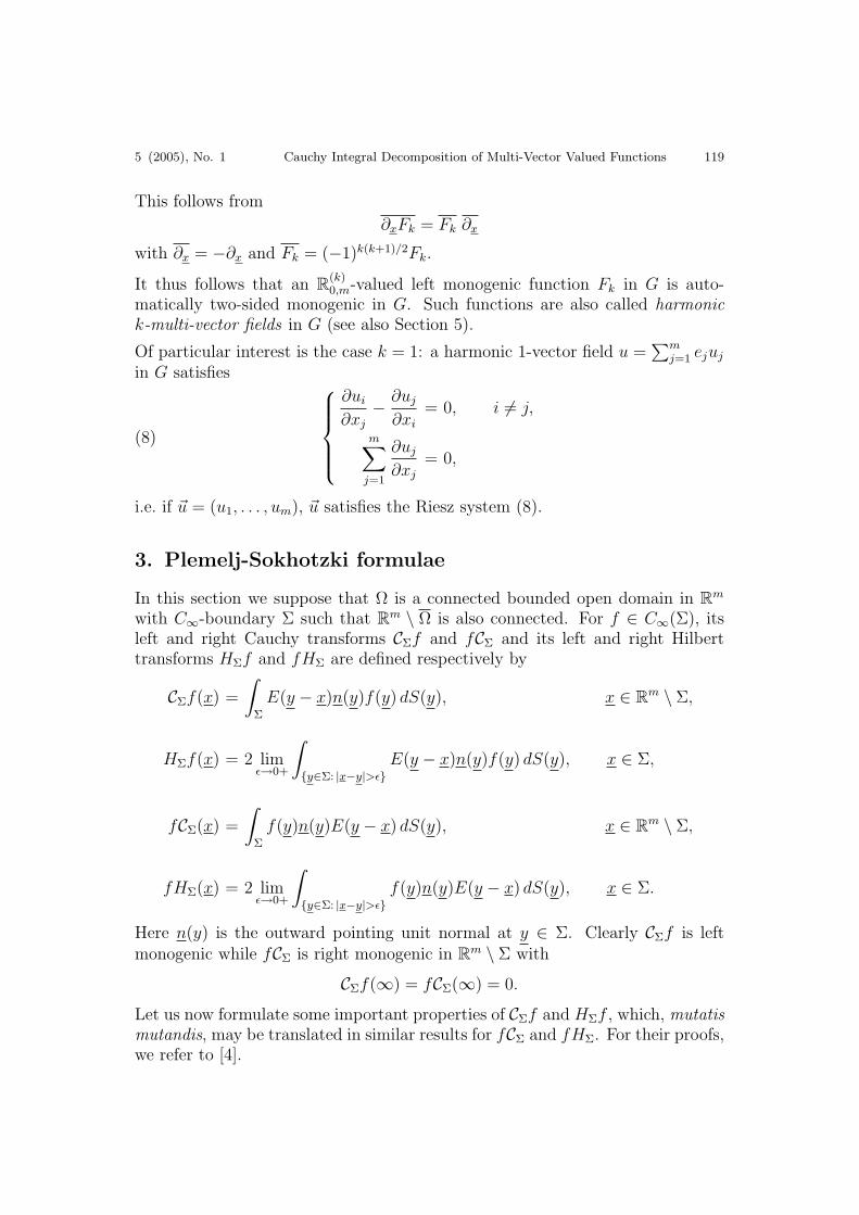
This follows from

∂xFk = Fk ∂x

with ∂x = −∂x and Fk = (−1)k(k+1)/2Fk.

It thus follows that an R(k)0,m-valued left monogenic function Fk in G is auto-

matically two-sided monogenic in G. Such functions are also called harmonick-multi-vector fields in G (see also Section 5).

Of particular interest is the case k = 1: a harmonic 1-vector field u =∑m

j=1 ejuj

in G satisfies

(8)

∂ui

∂xj

− ∂uj

∂xi

= 0, i 6= j,

m∑j=1

∂uj

∂xj

= 0,

i.e. if ~u = (u1, . . . , um), ~u satisfies the Riesz system (8).

3. Plemelj-Sokhotzki formulae

In this section we suppose that Ω is a connected bounded open domain in Rm

with C∞-boundary Σ such that Rm \ Ω is also connected. For f ∈ C∞(Σ), itsleft and right Cauchy transforms CΣf and fCΣ and its left and right Hilberttransforms HΣf and fHΣ are defined respectively by

CΣf(x) =

∫Σ

E(y − x)n(y)f(y) dS(y), x ∈ Rm \ Σ,

HΣf(x) = 2 limε→0+

∫y∈Σ: |x−y|>ε

E(y − x)n(y)f(y) dS(y), x ∈ Σ,

fCΣ(x) =

∫Σ

f(y)n(y)E(y − x) dS(y), x ∈ Rm \ Σ,

fHΣ(x) = 2 limε→0+

∫y∈Σ: |x−y|>ε

f(y)n(y)E(y − x) dS(y), x ∈ Σ.

Here n(y) is the outward pointing unit normal at y ∈ Σ. Clearly CΣf is leftmonogenic while fCΣ is right monogenic in Rm \ Σ with

CΣf(∞) = fCΣ(∞) = 0.

Let us now formulate some important properties of CΣf and HΣf , which, mutatismutandis, may be translated in similar results for fCΣ and fHΣ. For their proofs,we refer to [4].


(i) CΣf extends to C∞(Ω), i.e.

CΣf ∈ M(Ω) ∩ C∞(Ω).

(ii) If C+Σf denotes the trace of CΣf to Σ, i.e. for x ∈ Σ, if

C+Σf(x) = lim

Ω3x→xCΣf(x),

then

C+Σf(x) =

1

2(f(x) + HΣf(x)) .

(iii) HΣf ∈ C∞(Σ) and C+Σ (C+

Σf) = C+Σf .

Now let R > 0 be such that Ω ⊂ B(R) and put Ω∗ = B(R) \ Ω. Then Ω∗ is acompact, connected manifold with C∞-boundary Σ∗ = ∂B(R) ∪ Σ, whence forF ∈ C∞(Σ∗), Calderbank’s results [4, §§6–9] remain valid.

Putting for f ∈ C∞(Σ),

F (x) =

f(x), x ∈ Σ

0, x ∈ ∂B(R),

we thus have for the Cauchy and Hilbert transforms CΣ∗F and HΣ∗F that

CΣ∗F ∈ M(Ω∗) ∩ C∞(Ω∗).

Moreover, straightforward arguments lead to the following results.

(iv) For x ∈ Ω∗,

CΣ∗F (x) = −CΣf(x).

(v) For x ∈ Σ∗

C+Σ∗F (x) =

1

2(F (x) + HΣ∗F (x)) =

−CΣf(x), x ∈ ∂B(R)12(f(x)−HΣf(x)), x ∈ Σ.

It thus follows from (iv) and (v) that for x ∈ Σ,

C−Σf(x) = limRm\Ω3x→x

CΣf(x) =1

2(−f(x) + HΣf(x)) .

Putting Ω+ = Ω and Ω− = Rm\Ω, we obtain the following theorem by combiningthe foregoing results.

Theorem 3.1. Let Ω ⊂ Rm be an open bounded and connected domain withC∞-boundary Σ such that Rm \Ω is connected. Furthermore, let for f ∈ C∞(Σ),CΣf and HΣf be, respectively, the Cauchy and Hilbert transforms of f . Then

(i) CΣf ∈ M(Rm \ Σ) with CΣf(∞) = 0;(ii) HΣf ∈ C∞(Σ);


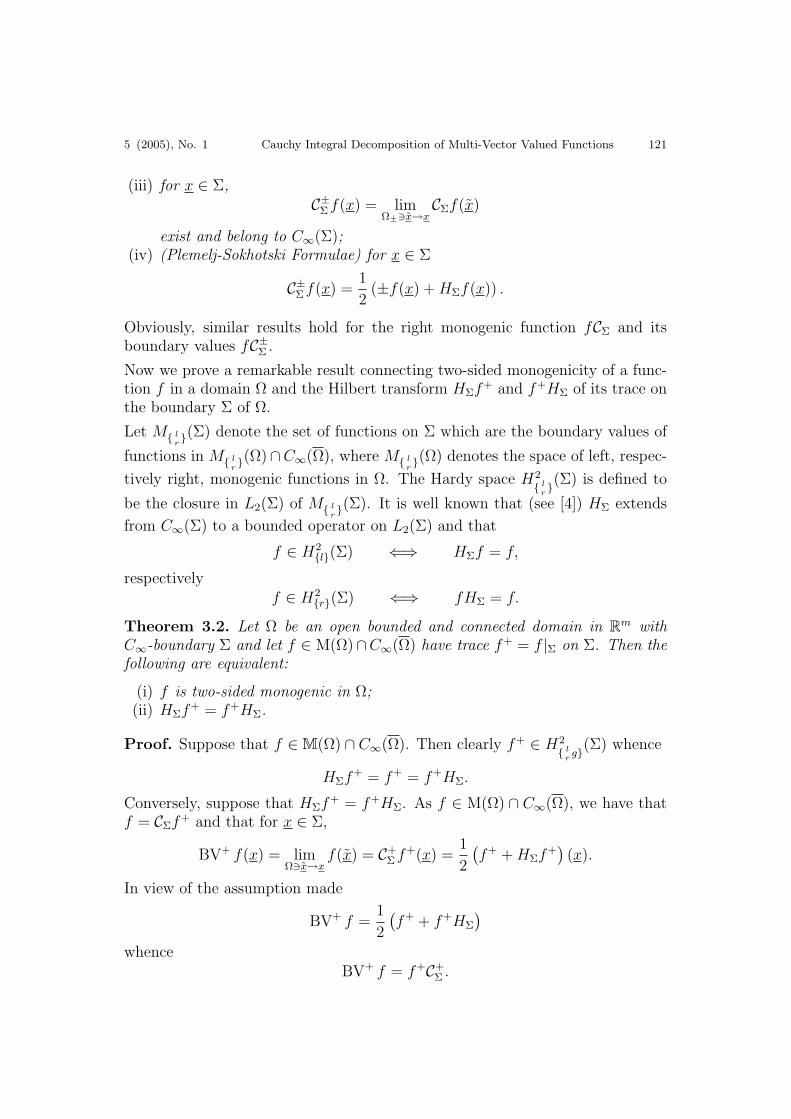
(iii) for x ∈ Σ,C±Σf(x) = lim

Ω±3x→xCΣf(x)

exist and belong to C∞(Σ);(iv) (Plemelj-Sokhotski Formulae) for x ∈ Σ

C±Σf(x) =1

2(±f(x) + HΣf(x)) .

Obviously, similar results hold for the right monogenic function fCΣ and itsboundary values fC±Σ .

Now we prove a remarkable result connecting two-sided monogenicity of a func-tion f in a domain Ω and the Hilbert transform HΣf+ and f+HΣ of its trace onthe boundary Σ of Ω.

Let M lr(Σ) denote the set of functions on Σ which are the boundary values of

functions in M lr(Ω)∩C∞(Ω), where M l

r(Ω) denotes the space of left, respec-

tively right, monogenic functions in Ω. The Hardy space H2 l

r(Σ) is defined to

be the closure in L2(Σ) of M lr(Σ). It is well known that (see [4]) HΣ extends

from C∞(Σ) to a bounded operator on L2(Σ) and that

f ∈ H2l(Σ) ⇐⇒ HΣf = f,

respectivelyf ∈ H2

r(Σ) ⇐⇒ fHΣ = f.

Theorem 3.2. Let Ω be an open bounded and connected domain in Rm withC∞-boundary Σ and let f ∈ M(Ω)∩C∞(Ω) have trace f+ = f |Σ on Σ. Then thefollowing are equivalent:

(i) f is two-sided monogenic in Ω;(ii) HΣf+ = f+HΣ.

Proof. Suppose that f ∈ M(Ω) ∩ C∞(Ω). Then clearly f+ ∈ H2 l

rg(Σ) whence

HΣf+ = f+ = f+HΣ.

Conversely, suppose that HΣf+ = f+HΣ. As f ∈ M(Ω) ∩ C∞(Ω), we have thatf = CΣf+ and that for x ∈ Σ,

BV+ f(x) = limΩ3x→x

f(x) = C+Σf+(x) =

1

2

(f+ + HΣf+

)(x).

In view of the assumption made

BV+ f =1

2

(f+ + f+HΣ

)whence

BV+ f = f+C+Σ .


Now put g = (BV+ f)CΣ. Then g is right monogenic in Ω and belongs to C∞(Ω),with

BV+ g = limΩ3x→x

g(x) = (f+C+Σ )C+

Σ = f+C+Σ = BV+ f.

Put h = f−g. Then h is harmonic in Ω and it belongs to C∞(Ω) with BV+ h = 0on Σ. The classical Dirichlet problem then implies that h ≡ 0 in Ω or f = gin Ω. Consequently f is also right monogenic in Ω.

Remark. Plemelj-Sokhotski type formulae

(9) C±Σf(x) =1

2(±f(x) + HΣf(x))

may also be obtained in the following cases.

(i) Σ ⊂ Rm is the graph of a Lipschitz function, Ω± are domains in Rm whichlie, respectively, above and below Σ and f ∈ Lp(Σ), 1 < p < +∞ (see[11, 12]). The relations (9) then hold for a.e. x ∈ Σ.

(ii) Σ is the boundary of a bounded Lipschitz domain and f belongs to theclass Lp(Σ), 1 < p < +∞ (see [8]). Again the relations (9) then hold fora.e. x ∈ Σ.

(iii) Ω is a bounded open domain in Rm such that its boundary Σ is a Liapunovhypersurface and f ∈ C0,α(Σ), 0 < α < 1 (see [10]). The relations (9) holdfor all x ∈ Σ. For f ∈ C0,α(Σ), the relations (9) remain valid in the casewhere Σ is an Ahlfors-David regular hypersurface, although a change in thedefinition of HΣ has to be carried out (see [1]).

(iv) Since in the case of f ∈ C0,α(Σ) (0 < α < 1), Σ being a Liapunov hyper-surface, (9) holds and (C+

Σ )2 = C+Σ on C0,α(Σ), Theorem 3.2 remains valid

for f ∈ M(Ω) ∩ C0,α(Ω).

4. A conservation law for two-sided monogenic functions

In this section a condition is established on the boundary value of a function fwhich is two-sided monogenic in Ω and belongs to C∞(Ω). This condition givesrise to a set of equivalent assertions concerning the Cauchy integral decomposi-tion of a k-multi-vector field Fk ∈ C∞(Σ).

4.1. The general case. Suppose that Ω is a connected open bounded do-main in Rm with C∞-boundary Σ. Furthermore, following Section 2, assumethat in a small ε-normal open neighborhood Σε of Σ, x ∈ Σε has local co-ordinates x = (ν, ω1, . . . , ωm−1) = (ν, ω) with respect to the orthonormal frame(n, ε1, . . . , εm−1) where

(i) x = n(x ⊥)ν(x) + x ⊥ with x ⊥ ∈ Σ, n = n(x ⊥) the unit normal at x ⊥ andν(x) = 〈n, x〉;

(ii) x ⊥ =∑m−1

j=1 εj〈εj, x〉, (ε1, . . . , εm−1) being an orthonormal basis of the tan-

gent space T (x ⊥) at x ⊥;


(iii) ω = (ω1, . . . , ωm−1) is a local C∞-coordinate system at x ⊥ on Σ.

As we have seen, the Dirac operator ∂x may be expressed as

∂x = n〈n, ∂x〉+ ∂‖x

where ∂‖x is the tangential Dirac operator with

∂‖x =∑j,i

εj Qji∂ωi.

For f ∈ C∞(Ω) we have that

∂xf = n〈n, ∂x〉f + ∂‖xf,(10)

f∂x = f〈n, ∂x〉n + f∂‖x.(11)

Furthermore, if f+ = f |Σ, then ∂‖xf |Σ = ∂ωf+ where

∂ω =∑j,i

εj Qji(0, ω)∂ωi.

Now suppose that f ∈ M(Ω) ∩ C∞(Ω). From ∂xf = 0 and f∂x = 0, it followsrespectively, that

〈n, ∂x〉f − n∂‖xf = 0,(12)

〈n, ∂x〉f − (f∂‖x)n = 0(13)

whence in Ω,n∂‖xf = (f∂‖x)n

or equivalently,

(14) n(∂‖xf)n + f∂‖x = 0.

We thus obtain from (14) that for f ∈ M(Ω) ∩ C∞(Ω), on Σ

(15) n(∂ωf+)n + f+∂ω = 0.

Relation (15) is called conservation law or (CL)-condition for f ∈ M(Ω)∩C∞(Ω).

Remark. The term “conservation law” is borrowed from electrodynamics. Thefree field Maxwell equations correspond to a bivector field f(x, t) in spacetimesatisfying the Hodge system or, equivalently, the two-sided monogenic system.Assume that one would have such a Maxwell field f(x, t) in a domain of the formΩ×R say, Ω ⊂ R3 and R the time axis, then the boundary value f(ω, t), ω ∈ ∂Ωhas the form nJ(ω, t) where n is the unit normal to ∂Ω and J(ω, t) is the currentgenerating the field f(ω, t). The conservation laws in our paper correspond inthis case to the conservation of electromagnetic charge i.e. divJ = 0.

Conversely, suppose that f ∈ M(Ω) ∩ C∞(Ω) satisfies the (CL)-condition (15).Put g = f∂x. Then combining (11) and (12) we have for g+, the restriction of gto Σ, that

(16) g+ = n(∂ωf+)n + f+∂ω.


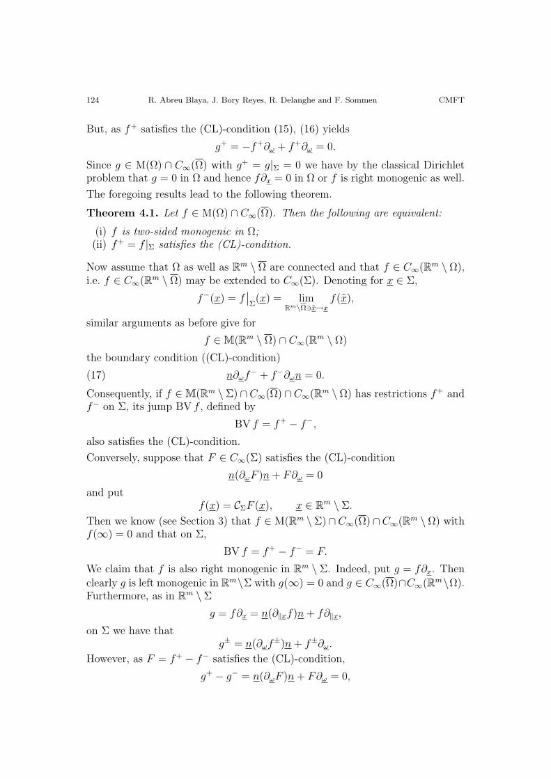
But, as f+ satisfies the (CL)-condition (15), (16) yields

g+ = −f+∂ω + f+∂ω = 0.

Since g ∈ M(Ω) ∩ C∞(Ω) with g+ = g|Σ = 0 we have by the classical Dirichletproblem that g = 0 in Ω and hence f∂x = 0 in Ω or f is right monogenic as well.

The foregoing results lead to the following theorem.

Theorem 4.1. Let f ∈ M(Ω) ∩ C∞(Ω). Then the following are equivalent:

(i) f is two-sided monogenic in Ω;(ii) f+ = f |Σ satisfies the (CL)-condition.

Now assume that Ω as well as Rm \ Ω are connected and that f ∈ C∞(Rm \ Ω),i.e. f ∈ C∞(Rm \ Ω) may be extended to C∞(Σ). Denoting for x ∈ Σ,

f−(x) = f∣∣Σ(x) = lim

Rm\Ω3x→xf(x),

similar arguments as before give for

f ∈ M(Rm \ Ω) ∩ C∞(Rm \ Ω)

the boundary condition ((CL)-condition)

(17) n∂ωf− + f−∂ωn = 0.

Consequently, if f ∈ M(Rm \Σ) ∩C∞(Ω) ∩C∞(Rm \Ω) has restrictions f+ andf− on Σ, its jump BV f , defined by

BV f = f+ − f−,

also satisfies the (CL)-condition.

Conversely, suppose that F ∈ C∞(Σ) satisfies the (CL)-condition

n(∂ωF )n + F∂ω = 0

and putf(x) = CΣF (x), x ∈ Rm \ Σ.

Then we know (see Section 3) that f ∈ M(Rm \Σ) ∩C∞(Ω) ∩C∞(Rm \Ω) withf(∞) = 0 and that on Σ,

BV f = f+ − f− = F.

We claim that f is also right monogenic in Rm \ Σ. Indeed, put g = f∂x. Then

clearly g is left monogenic in Rm\Σ with g(∞) = 0 and g ∈ C∞(Ω)∩C∞(Rm\Ω).Furthermore, as in Rm \ Σ

g = f∂x = n(∂‖xf)n + f∂‖x,

on Σ we have thatg± = n(∂ωf±)n + f±∂ω.

However, as F = f+ − f− satisfies the (CL)-condition,

g+ − g− = n(∂ωF )n + F∂ω = 0,


whence on Σg+ = g−.

By virtue of the Painleve Theorem (see [1]), g is left monogenic in Rm. But, asg(∞) = 0, by means of the Liouville Theorem (see [1]), g ≡ 0 in Rm \ Σ and sof ∈ M(Rm \ Σ). This gives us the following result.

Theorem 4.2. Let Ω ⊂ Rm be an open bounded and connected set withC∞-boundary Σ such that Rm \ Ω is connected. Furthermore, let F ∈ C∞(Σ)satisfy the (CL)-condition

n(∂ωF )n + F∂ω = 0.

If f ∈ M(Rm \ Σ) ∩ C∞(Ω) ∩ C∞(Rm \ Ω) with f(∞) = 0 is such that its jumpBV f = f+ − f− = F , then f = CΣF .

Proof. We have already shown that CΣF satisfies all properties of the givenfunction f . The Painleve and Liouville Theorems then imply that f = CΣF .

4.2. The multi-vector case. Let Ω be again a bounded open and connected

subset of Rm such that Rm\Ω is connected. Furthermore, let Fk be an R(k)0,m-valued

C∞-function on Σ. If Fk satisfies the (CL)-condition

n(∂ωFk)n + Fk∂ω = 0,

then we know by virtue of Theorem 4.2 that f = CΣFk is two-sided monogenicin Rm \ Σ.

Similar arguments as used in proving the equivalence of (ii), (iii) and (iv) in[1, Theorem 4.1] then imply that f is a harmonic k-multi-vector field in Rm \ Σ

with f(∞) = 0. Consequently, f± are also R(k)0,m-valued on Σ and by virtue of

Theorem 3.1, they belong to C∞(Σ) with

Fk = f+ − f−.

By means of the Plemelj-Sokhotski formula

f+ =1

2(Fk + HΣFk) ,

whence HΣFk is also R(k)0,m-valued on Σ with HΣFk ∈ C∞(Σ).

Conversely, suppose that for an R(k)0,m-valued C∞-function Fk on Σ, the function

HΣFk is also R(k)0,m-valued. Again put f = CΣFk and split f into its l-vector parts

fl = [CΣFk]l, l = k − 2, k, k + 2, i.e.

(18) f = fk−2 + fk + fk+2.

As f is left monogenic in Ω, ∆f = 0 in Ω and hence also ∆fl = 0, l = k−2, k, k+2.Furthermore, as by the Plemelj-Sokhotski formulae

f± =1

2(±Fk + HΣFk) ,


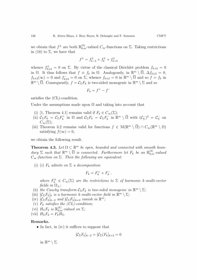
we obtain that f± are both R(k)0,m-valued C∞-functions on Σ. Taking restrictions

in (18) to Σ, we have that

f± = f±k−2 + f±k + f±k+2

whence f±k±2 = 0 on Σ. By virtue of the classical Dirichlet problem fk±2 = 0

in Ω. It thus follows that f ≡ fk in Ω. Analogously, in Rm \ Ω, ∆fk±2 = 0,fk±2(∞) = 0 and f−k±2 = 0 on Σ, whence fk±2 = 0 in Rm \ Ω and so f = fk in

Rm \ Ω. Consequently, f = CΣFk is two-sided monogenic in Rm \ Σ and so

Fk = f+ − f−

satisfies the (CL)-condition.

Under the assumptions made upon Ω and taking into account that

(i) [1, Theorem 4.1] remains valid if Fk ∈ C∞(Σ);(ii) CΣFk = CΣF+

k in Ω and CΣFk = CΣF−k in Rm \ Ω with (C−Σ )2 = C−Σ on

C∞(Σ);(iii) Theorem 3.2 remains valid for functions f ∈ M(Rm \ Ω) ∩ C∞(Rm \ Ω)

satisfying f(∞) = 0,

we obtain the following result.

Theorem 4.3. Let Ω ⊂ Rm be open, bounded and connected with smooth boun-

dary Σ such that Rm \ Ω is connected. Furthermore let Fk be an R(k)0,m-valued

C∞-function on Σ. Then the following are equivalent:

(i) (i) Fk admits on Σ a decomposition

Fk = F+k + F−

k ,

where F±k ∈ C∞(Σ) are the restrictions to Σ of harmonic k-multi-vector

fields in Ω±;(ii) the Cauchy transform CΣFk is two-sided monogenic in Rm \ Σ;(iii) [CΣFk]k is a harmonic k-multi-vector field in Rm \ Σ;(iv) [CΣFk]k−2 and [CΣFk]k+2 vanish in Rm;(v) Fk satisfies the (CL)-condition;

(vi) HΣFk is R(k)0,m-valued on Σ;

(vii) HΣFk = FkHΣ.

Remarks.

• In fact, in (iv) it suffices to suppose that

[CΣFk]k−2 = [CΣ(Fk]k+2 = 0

in Rm \ Σ.


• If Fk ∈ (C∞(Σ), then for x ∈ Rm \ Σ (see (also [1]):

[CΣFk]k−2(x) =

∫Σ

E(y − x) • (n(y) • Fk(y)) dS(y),

[CΣFk]k+2(x) =

∫Σ

E(y − x) ∧ (n(y) ∧ Fk(y)) dS(y).

Consequently, requiring that [CΣFk]k±2 = 0 in Rm \ Σ is equivalent toimposing the conditions∫

Σ

E(y − x) • (n(y) • Fk(y)) dS(y) = 0,(19) ∫Σ

E(y − x) ∧ (n(y) ∧ Fk(y)) dS(y) = 0.(20)

Call Nk(C∞(Σ)) the subspace of C∞(Σ) consisting of those R(k)0,m-valued

C∞-functions Fk on Σ for which the conditions (19) and (20) are satis-fied and call Mk(Ω+ ∪ Ω−) the space of harmonic k-multi-vector fields Fk

in Ω+ ∪ Ω− with Fk(∞) = 0. Then Theorem 4.3 tells us that CΣ mapsNk(C∞(Σ)) into Mk(Ω+ ∪ Ω−).In the special case where k = 1, for any 1-valued C∞-function F1 on Σ, thecondition (19) is automatically satisfied since on Σ

E(y − x) • (n(y) • F1(y)) ≡ 0.

Consequently N1(C∞(Σ)) consists of those F1 ∈ C∞(Σ) for which (20)holds.Theorem 4.3 implies that CΣ maps N1(C∞(Σ)) into M1(Ω+∪Ω−), the spaceof harmonic vector fields in Ω+ ∪ Ω− which vanish at ∞.

• In [1, Theorem 4.1] , the equivalent conditions (i)-(iv) from Theorem 4.3were obtained in the case where Fk ∈ C0,α(Σ), Σ being an Ahlfors-Davidregular hypersurface in Rm.Denote by N1(C

0,α(Σ)) the space of 1-vector valued functions on Σ whichbelong to C0,α(Σ), and which satisfy the condition (20). Then CΣ mapsN1(C

0,α(Σ)) into M1(Ω+∪Ω−)∩C0,α(Ω+∪Ω−). A similar result, althoughformulated in different terms, was obtained by M. Shapiro in [14] and thisin the case where Σ is a Liapunov hypersurface. As is well known, anyLiapunov hypersurface is an Ahlfors-David regular hypersurface.

• In [7, Theorem 3] Dyn’kin gave an explicit representation formula for theharmonic k-forms η±k in Ω± which lead to the decomposition

ηk = η+k + η−k

of a k-form on Σ satisfying the conditions (A) and (B). A careful analysisof this formula shows that, by means of the isomorphism Θ (see Lemma5.1), ηk = Θ[CΣFk]k, where Fk satisfies the condition (i) of Theorem 4.3.


Consequently, Dyn’kin’s integral representation formulae for harmonic k-forms can be obtained from the Cauchy integral formula in Clifford analysis,by projecting the latter formula onto its k-vector part. Notice in this re-gard that a Cauchy integral formula specific to harmonic k-forms was alsoderived directly from the Clifford analysis setting in [9].

5. Dyn’kin’s condition (A) in Clifford analysis

In this section it is shown that Dyn’kin’s Condition (A) on the boundary value ofa harmonic k-form is equivalent to the conservation law for the boundary valueof the corresponding k-multi-vector field.

5.1. Harmonic k-multivector fields and k-forms. If G is an open subset ofRm, then there is a natural vectorial isomorphism Θ between the spaces Ek(G)and Λk(G) of, respectively, smooth k-multi-vector fields and smooth k-forms inG: for Fk =

∑|A|=k FAeA, put

ΘFk = ηk =∑|A|=k

ηAdxA

where for all A = i1, . . . , ik ⊂ 1, . . . ,m, ηA = FA and

dxA = dxi1 ∧ · · · ∧ dxik .

This isomorphism Θ may also be obtained as follows: consider the form

dx =m∑

j=1

dxjej.

Then clearly for each k ∈ 1, . . . ,m,

dxk = k!∑|A|=k

eAdxA.

Using the classical inner product 〈·, ·〉 on k-multi-vectors, we thus obtain thefollowing lemma.

Lemma 5.1. If Fk ∈ Ek(G), then

ΘFk = ηk =1

k!〈Fk, dxk〉.

Now suppose that Fk is left-and hence two-sidedmonogenic in G, i.e. ∂xFk = 0in G. Then, as

∂xFk = ∂x • Fk + ∂x ∧ Fk,

we obtain that

(21) ∂xFk = 0 ⇐⇒

∂x ∧ Fk = 0,

∂x • Fk = 0.


Putting ηk = ΘFk, it is easily verified that (21) is equivalent to

(22)

dηk = 0,

d∗ηk = 0,

or to

(23)

dηk = 0,

d ∗ ηk = 0.

In turn (23) is equivalent to

(24)

∂x ∧ Fk = 0,

∂x ∧ eMFk = 0,

since

0 = dηk = d(ΘFk),

0 = d ∗ ηk = d(Θ(eMFk)).

As already mentioned in the introduction, a k-multi-vector field Fk which ismonogenic in G — or equivalently a k-form ηk which satisfies the Hodge-deRham system (22) in G — is called harmonic in G.

5.2. Dyn’kin’s condition (A) for harmonic k-forms versus the (CL)-condition for harmonic k-multi-vector fields. Let Ω be a bounded openand connected subset of Rm having as boundary the C∞-surface Σ and let forε > 0, Σε be an ε-normal open neighborhood of Σ (see Section 2).

In terms of the coordinate system (ν, ω1, . . . , ωm−1) we obtain that in Ω ∩ Σε,

dx =∂x

∂νdν +

m−1∑j=1

∂x

∂ωj

dωj = ndν +∑i,j

Ki,jεj dωi = n dν +m−1∑j=1

εjφj

where the Ki,j’s are C∞-functions in (ν, ω) and the φj’s are 1-forms dependingonly on dω1, . . . , dωm−1.

For k ∈ 1, . . . ,m fixed, we thus get

dxk =

(n dν +

m−1∑j=1

εjφj

)k

=

(m−1∑j=1

εjφj

)k

+ kn dν

(m−1∑j=1

εjφj

)k−1

.

Here we used the commutation relation

(n dν)

(m−1∑j=1

εjφj

)=

(m−1∑j=1

εjφj

)(n dν) .

Now let Fk ∈ Ek(Ω)∩C∞(Ω), i.e. Fk is a smooth k-multi-vector field in Ω whichis extendable to C∞(Σ). In terms of the orthonormal frame (n, ε1, . . . , εm−1), thefunction Fk may be written in Ω ∩ Σε as

(25) Fk = F (k) + nF (k−1)


where F (l), l = k, k − 1, are l-multi-vector fields over (ε1, . . . , εm−1).

Applying Lemma 5.1 to (25) we get

ηk = ΘFk = ΘF (k) + Θ(nF (k−1))

=1

k!

⟨F (k),

(m−1∑j=1

εjφj

)k⟩+

kdν

k!

⟨nF (k−1), n

(m−1∑j=1

εjφj

)k−1⟩= η(k) + dν η(k−1).

Here η(l), l = k, k − 1, are l-forms over (dω1, . . . , dωm−1).

Now suppose ηk = ΘFk is harmonic in Ω, i.e. it satisfies the Hodge-de Rhamsystem (23). As ηk is assumed to be extendable to C∞(Σ), by restricting to theboundary, we immediately obtain Dyn’kin’s Condition (A) (see [7]), namely

dηk = 0 (A1)d ∗ ηk = 0 (A2)

.

We now claim that in Clifford analysis terms, Condition (A) is equivalent to the(CL)-condition for the boundary value F+

k = Fk|Σ of the harmonic k-multi-vectorfield Fk (see (15))

n(∂ωF+k )n + F+

k ∂ω = 0.

Let us prove this statement in the case where k is odd, the proof of the case keven being similar. In order to avoid tedious calculations, we only give a sketchof the proof. Let us first show how the (CL)-condition may be derived fromCondition (A). In fact, we shall establish separately conditions upon F+

k whichare equivalent to, respectively, the Conditions (A1) and (A2). Let us start bytranslating Condition (A1).

As we have seen (see (24)), Condition (A1) also reads:

d(ΘFk)∣∣Σ

= (Θ(∂x ∧ Fk))∣∣Σ

= 0.

As k is odd,

∂x ∧ Fk =1

2(∂xFk − Fk∂x) =

1

2[∂x, Fk].

Moreover, as [∂x, Fk] is a (k + 1)-multi-vector field, we may write it in the form(see (25))

(26) [∂x, Fk] = F (k+1) + nF (k)

where F (k+1) and F (k) are constructed over (ε1, . . . , εm−1).

By virtue of (26)

(Θ[∂x, Fk])∣∣Σ

=(ΘF (k+1) + dνΘF (k)

) ∣∣Σ

=(ΘF (k+1)

) ∣∣Σ

= Θ(F (k+1)∣∣Σ).

But, k being odd, we have that

nF (k+1) = F (k+1)n,

nF (k) = −F (k)n,


whence from (26) we get

(27) F (k+1)∣∣Σ

=

(−n

2n, [∂x, Fk]

) ∣∣∣∣Σ

.

Condition (A1), namelyd(ΘFk)

∣∣Σ

= 0

is thus equivalent toΘ(F (k+1)|Σ) = 0

or to F (k+1)|Σ = 0.

In view of (27) it is hence also equivalent to

n, [∂x, Fk]∣∣Σ

= 0.

Now writing Fk in the form (see also (25))

Fk = F (k) + nF (k−1),

by using the relation (7), straightforward calculations lead to

(A1) ⇐⇒ (CL1)

where (CL1) is given by

(28) 0 = n, [∂x, Fk]∣∣Σ

= n, [∂‖x, Fk]∣∣Σ

= n, [∂ω, F+k ].

Analogously it may be shown that

(A2) ⇐⇒ (CL2)

where (CL2) is given by

(29) 0 = [n, ∂x, Fk]∣∣Σ

= [n, ∂‖x, Fk]∣∣Σ

= [n, ∂ω, F+k ].

Obviously, (28) and (29) imply the (CL)-condition

n(∂ωF+k )n + F+

k ∂ω = 0.

Conversely, suppose that Fk is a harmonic k-multi-vector field in Ω which extendsto C∞(Σ) and which is such that its trace on the boundary F+

k = Fk|Σ satisfiesthe (CL)-condition

n(∂ωF+k )n + F+

k ∂ω = 0

or equivalently,

(30) n(∂ωF+k ) = (F+

k ∂ω)n.

As F+k is R(k)

0,m-valued, ∂ωF+k , which splits into a (k+1)- and a (k−1)-multivector,

may be written as

(31) ∂ωF+k = A + nB,

where

A = A(k+1) + A(k−1),

B = B(k) + B(k−2).


Here the A(l)’s, l = k−1, k +1, and B(j)’s, j = k, k−2, are l- and j-multi-vectorfields constructed over ε1, . . . , εm−1.

Put σ = (−1)k(k+1)/2. On the one hand, we obtain that

(32) ∂ωF+k = −σF+

k ∂ω

while on the other hand

∂ωF+k = A−Bn = A

(k+1)+ A

(k−1) −B(k)

n−B(k−2)

n.

But now, for k odd,

A(k+1)

= σA(k+1),

A(k−1)

= −σA(k−1)

while

B(k)

= σB(k),

B(k−2)

= −σB(k−2).

Taking also into account that A(k+1)n = nA(k+1), it follows from (30), (31) and(32) that A(k+1) = 0 and B(k−2) = 0.

Now the (k + 1)-vector A(k+1) is the tangent part of [∂ωF+k ]k+1. But

[∂ωF+k ]k+1 = ∂ω ∧ F+

k =1

2[∂ω, F+

k ].

HenceA(k+1) = −n

2n, [∂ω, F+

k ]

and so A(k+1) = 0 leads to

n, [∂ω, F+k ] = n, [∂‖x, Fk]

∣∣Σ

= 0,

thus giving condition (CL1) (see (29)).

Similarly, from B(k−2) = 0, it follows that

[n, ∂ω, F+k ] = [n, ∂‖x, Fk]

∣∣Σ

= 0

thus implying condition (CL2) (see (30)).

Consequently, the (CL)-condition implies condition (A).

We may thus conclude with the following theorem.

Theorem 5.1. Let Ω be an open, bounded and connected subset of Rm having theC∞- surface Σ as boundary. Furthermore, let Fk be a harmonic k-multi-vectorfield in Ω which is extendable to C∞(Σ) and has the trace F+

k = Fk|Σ on Σ.

If ηk = ΘFk is the corresponding harmonic k-form, thendηk

∣∣Σ

= 0d∗ηk

∣∣Σ

= 0⇐⇒ n(∂ωF+

k )n + F+k ∂ω = 0

i.e. Dyn’kin’s Condition (A) and the (CL)-condition are equivalent.


Remarks.

• For smooth differential forms in Ω which are extendable to C∞(Σ), Dyn’kin’sConditions (A1) and (A2) are natural, since closedness of differential formsin Ω is inherited when restricting to the boundary Σ.For a k-multi-vector field Fk ∈ M(Ω) ∩ C∞(Ω), the conservation law (CL)for the trace F+

k = Fk|Σ indicates the possibility of eliminating the normalderivative at the boundary.

• Let again Fk ∈ Ek(Ω) ∩ C∞(Σ) and let ηk = ΘFk. Then

Θ(∂x ∧ Fk) = dηk = d(ΘFk).

It should however be stressed that

(Θ(∂x ∧ Fk))∣∣Σ6= Θ((∂x ∧ Fk)

∣∣Σ).

That is the reason why, in deriving the (CL)-condition from Condition (A),we wrote out ∂x ∧ Fk in Ω ∩ Σε as (see (26))

∂x ∧ Fk = F (k+1) + nF (k).

This observation indicates an essential difference between the calculus ofdifferential forms and the calculus of multi-vector fields when taking traceson the boundary of a domain.

Acknowledgement. This paper was written while the first two authors wereguests at the Department of Mathematical Analysis of Ghent University. Theywish to thank all members of this Department for their kind hospitality. Theauthors would like to thank the referees for their valuable suggestions.

References

1. R. Abreu, J. Bory, R. Delanghe and F. Sommen, Harmonic multivector fields and theCauchy integral decomposition in Clifford analysis, Bull. Belg. Math. Soc. 11 (2004), 95–110.

2. L. A. Aizenberg and Sh. A. Dautov, Differential Forms Orthogonal to Holomorphic Func-tions or Forms, AMS, Providence, R.I., 1983.

3. A. Andreotti and C. D. Hill, E. E. Levi convexity and the H. Lewy problem, I, Ann. ScuolaNorm. Sup. Pisa Cl. Sci. 26 (1972), 325–363.

4. D. Calderbank, Clifford analysis for Dirac operators on manifolds with boundary, Max-Planck-Institut fur Mathematik, MPI 96–131, 1996.

5. R. Delanghe, F. Sommen and V. Soucek, Clifford Algebra and Spinor-Valued Functions,Kluwer, Dordrecht, 1992.

6. E. Dyn’kin, Cauchy integral decomposition for harmonic vector fields, Complex VariablesTheory Appl. 31 (1996), 165–176.

7. , Cauchy integral decomposition for harmonic forms, J. Anal. Math. 73 (1997),165–186.

8. J. Gilbert and M. Murray, Clifford Algebras and Dirac Operators in Harmonic Analysis,Cambridge University Press, Cambridge, 1991.


9. J. Gilbert, J. Hogan and J. Lakey, Frame decompositions of form-valued Hardy spaces, in:J. Ryan (ed.), Clifford algebras in analysis and related topics, CRC Press, Boca Raton,1996, 239–259.

10. V. Iftimie, Fonctions hypercomplexes, Bull. Math. Soc. Sci. Math. Repub. Soc. Roum.Nouv. Ser. 9 (1965), 279–332.

11. A. McIntosh, Clifford algebras, Fourier theory, singular integrals, and harmonic functionson Lipschitz domains, in: J. Ryan (ed.), Clifford algebras in analysis and related topics,CRC Press, Boca Raton, 1996, 33–87.

12. M. Mitrea, Clifford Wavelets, Singular Integrals, and Hardy Spaces, Lecture Notes inMathematics 1575, Springer-Verlag, Berlin, 1994.

13. M. Riesz, Clifford Numbers and Spinors (Chapters I–IV) Lecture Series, No. 38, Institutefor Physical Science and Technology, Maryland, 1958.

14. M. Shapiro, On the conjugate harmonic functions of M. Riesz–E. Stein–G. Weiss, in:S. Dimiev and K. Sekigawa (Eds), Topics in omplex analysis, differential geometry andmathematical physics, World Sci. Publishing, 1997, 8-32.

15. E. Stein and G. Weiss, On the theory of harmonic functions of several variables, I: Thetheory of Hp-spaces, Acta Math. 103 (1960), 25–62.

Ricardo Abreu Blaya E-mail: [email protected]: Faculty of Mathematics and Informatics, University of Holguın, Holguın 80100,Cuba.

Juan Bory Reyes E-mail: [email protected]: Department of Mathematics, University of Oriente, Santiago de Cuba 90500, Cuba.

Richard Delanghe E-mail: [email protected]: Department of Mathematical Analysis, University of Ghent, Galglaan 2, B-9000Gent, Belgium.

Frank Sommen E-mail: [email protected]: Department of Mathematical Analysis, University of Ghent, Galglaan 2, B-9000Gent, Belgium.

Cauchy Integral Decomposition of MultiVector Valued Functions on Hypersurfaces

Documents

Transcript of Cauchy Integral Decomposition of MultiVector Valued Functions on Hypersurfaces