Cauchy Distribution for Jitter in IP Networks

L. Rizo1, D. Torres1, J. Dehesa1, D. Muñoz2 1CINVESTAV; Unidad Jalisco

2ITESM; Center for Electronics and Telecommunications lrizo, dtorres , jdehesa {@gdl.cinvestav.mx}, dmunoz@itesm.mx

Abstract In many real-time applications the Quality of Service (QoS ) is dominated by jitter. In this paper RTT (Round Trip Time) measurements were collected in order to find a probabilistic jitter model. From collected measurements the tail index was close to unit, this relates us to Cauchy's distribution. In this paper we show that the jitter has direct influence in the network performance. The purpose of this paper is to show how jitter dispersion affects the QoS in some applications. Keywords: Jitter, Cauchy distribution, QoS. 1. Introduction The transmission of multimedia information through Internet, with its policy of the best effort in the packet delivered, has been increased in the last years. Each multimedia application has its own requirements for a good performance. According to ITU [17], Internet could be evaluated in terms of some metrics such as: packet loss, jitter, One Way Delay (OWD) and bandwidth. In this work, we determine the negative effects of jitter for some applications. For this purpose Round Trip Time (RTT) measurements to different countries were collected. There are many works where jitter is modeled: In [1] Fulton and Li present an analytic study about jitter on Asynchronous Transfer Mode (ATM) networks, determining the jitter Probability Density Function (PDF) and its autocorrelation function for specific background traffic environments; the results were compared with simulations. Mansour and Patt-Sharmir proposed, in [2], an algorithm that uses a certain buffer size previously calculated in order to guarantee the QoS. Qiong and Mills [3] propose an algorithm to predict jitter on transport layer. Their model was based on Chebyshev’s inequality; the results of that work are applicable to TCP. An evaluation of the relationship between jitter and the characteristics of background traffic (using Interrupt Bernoulli process as traffic model) such as burstiness, traffic load and traffic burst length was presented in [4], where Zheng et al. analyze the jitter effects. A work of jitter generator based on Laplace distribution was developed by Daniel et al. [5]; nevertheless the RTT measurements collected by us from Mexico to: France,

Argentina, Japan and Australia do not agree with this statement. Under our knowledge there are no works that associate the jitter of IP networks with the Cauchy distribution. The motivation of this paper is to find a jitter model and a QoS metric. The remainder of this work is organized as follow: section 2 presents measurement methodologies and environmental. Section 3 describes jitter model. Section 4 presents the results. Section 5 shows the impact of the jitter on QoS and finally the section of concluding remarks. 2. Measurements In this section we describe the measurement environment to obtain several packet delays. 2.1 Environment

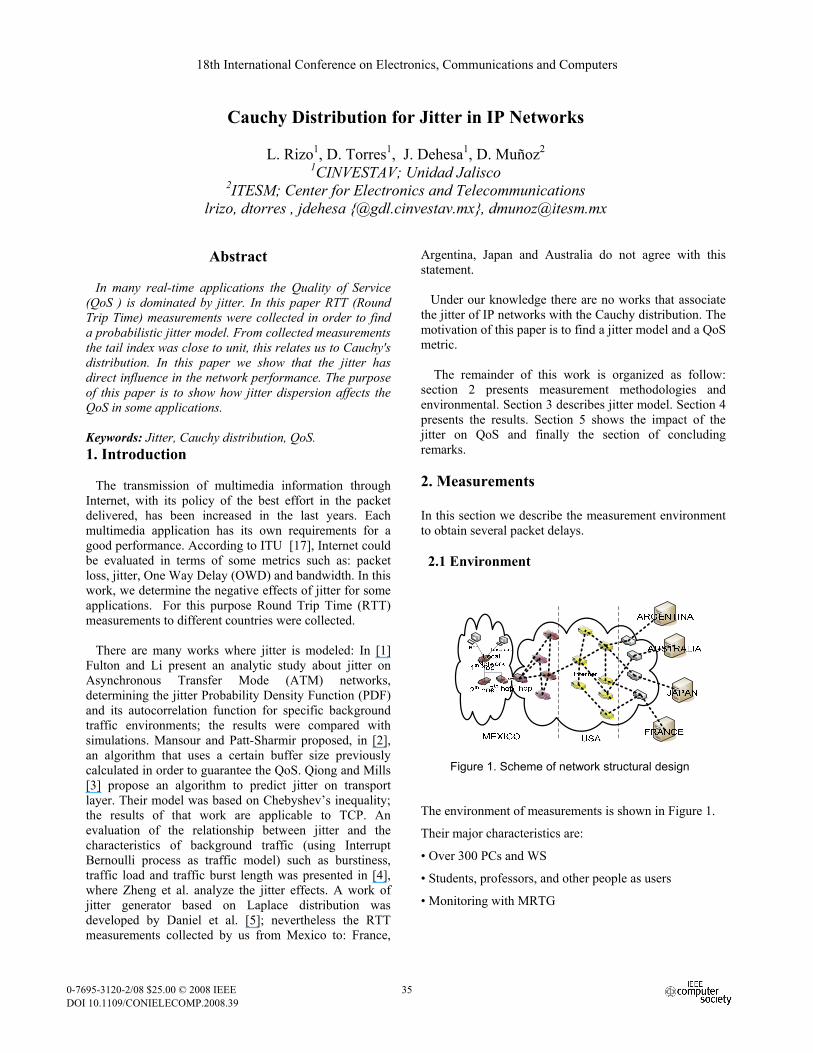
Figure 1. Scheme of network structural design The environment of measurements is shown in Figure 1.

Their major characteristics are:

• Over 300 PCs and WS

• Students, professors, and other people as users

• Monitoring with MRTG

18th International Conference on Electronics, Communications and Computers

0-7695-3120-2/08 $25.00 © 2008 IEEEDOI 10.1109/CONIELECOMP.2008.39

35

• Period of observation from 5 March 2006 to 15 May

2006

• Monday and Friday are identified as the days with

highest traffic loads

• Sunday was the day with lowest load

2.2 Sending Packet Algorithm The RTT traces with a duration of one day were collected and analyzed. The capture was handling by MPING program which sends/receives ICMP (Internet Control Message Protocol) packets (64 bytes). We collect RTT measurements for hop 1, hop 2,…, hop N consecutively; where the interdeparture time were management by a Linux interrupt, “ualarm”. Two scenarios were considered: low and high local load (Sunday and Monday respectively). Table 1 shows the paths, and periods of measurements. These measurements are available in [6]. The number of analyzed samples is 24 millions approximately.

Measurement set

Source-Destination

Ts Measurement period (2006)

A Mex-EUA-Argentina 620 ms Sun Mar 05th 00:00:00 –

Sun Mar 05th 23:59:05

B Mex-EUA-Argentina 620 ms Mon Mar 06th 00:00:00 –

Mon Mar 06th 23:59:05

C Mex-EUA-Australia 420 ms Sun Apr 09th 02:53:56 –

Mon Apr 10th 02:17:07

D Mex-EUA-Australia 420 ms Mon Apr 10th 02:17:07–

Tue Apr 11th 01:41:53

E Mex-EUA-Japon 580 ms Sun Apr 23th 00:09:00 –

Mon Apr 24th 00:05:03

F Mex-EUA-Japon 580 ms Mon Apr 24th 00:05:05 –

Tue Apr 25th 00:19:23

G Mex-EUA-Francia 420 ms Sun May 14th 00:11:32 -

Mon May 15th 00:05:24

H Mex-EUA-Francia 420 ms Mon May 15th 00:05:24 -

Tue May 16th 00:17:13

Table 1. Source, destination and period of the measurements

3. Jitter Model Jitter is defined here as the difference between the delays of packet k and k-1 at two different measurement points. In the ideal conditions this is a constant. However due to queuing waiting time in routers and route changes, packets experiment delay variation (jitter)

( ) ( ) ( 1)J k D k D k= − − (1) When jitter is less than zero a packet clustering phenomenon occurs which degrades QoS, and if jitter is greater than zero there is packet spreading that will require an increment of buffer size in order to compensate it. A heavy tail random variable is defined by its survival function as:

,1)( αxxXP ≈> ∞→x (2)

where: α is the tail index. Several studies show evidence that the network traffic exhibits long range dependence characteristics [7][13][14]. This implies according with [8], that waiting time in the queue will be heavy tailed. Therefore, it leads to think in a heavy tail behavior of delays and jitter. As r.v. with heavy tail distributions have infinite variance, then they can only converge to an alpha-stable distribution (considering the generalization of the central limit theorem). If two consecutive probe packets arrive at the queue in different busy periods, then its delay are independent. Based on observations, most of the multimedia applications have an interdeparture time greater than the queue busy period. Alpha stability theory states that for two independent and alpha-stable variables, their difference is also alpha stable. Therefore, based on the characteristics of ( )D k , the jitter ( )J k becomes also alpha stable. As the jitter definition used here implies a symmetrical r.v. then the employment of a symmetrical distribution is convenient. If 1α = , then Cauchy distribution can be used for the jitter. A r.v. X(t) is said to has a Cauchy distribution if its Cumulative Distribution Function (CDF) is given by following equation:

36

arctan1( )2

x

P X xγ

π

⎛ ⎞⎜ ⎟⎝ ⎠≤ = + (3)

where: γ is the scale parameter. 3.1 Estimation of the Tail Index There are some estimators of tail index. In this work we use standard Hill´s estimator and others three variants. 3.1.1. Standard Hill Estimator (SH) The Hill's estimator is a statistical tool, that estimates the index of tail,α , from samples of a process ( ) nX n N∈ , considering that the process is

stationary and its distribution function ( )F satisfies (2). Ordering the samples as 1 2 ... ...k nX X X X≥ ≥ ≥ , the

estimation of order k , ˆ ( )SH kα , is given by:

1

11

1ˆ ( ) log , for 1,..., 1.k iSH i

k

Xk k nk X

α−

=+

⎛ ⎞= = −⎜ ⎟⎝ ⎠∑ (4)

The Hill's estimator requires 1k + data and generates a vector of length k . One of the main difficulties of the Hill's estimator is to determine k . This is due to α̂ is sensitive to the number of used samples. 3.1.2. Smoothing Hill Estimator (SM) To make Hill's estimator less sensitive to k Resnick et.al. [10] suggest a smoothing technique. The smoothing procedure is an averaging of the standard Hill estimations:

1

1ˆ ˆ( , ) ( ), for 1( 1)

ukSM smooth p k

k u p uu k

α α= +

= >− ∑ (5)

With this averaging the Hill's estimations were smoothed producing a result less sensitive to the number of samples. 3.1.3. Alternative Hill Estimator (AH) Resnick and Stâricâ [10] suggested a simple modification called alternative plotting. Instead of

plotting ( ){ },, ,1 1k nk H k n≤ ≤ − , they construct the

alternative Hill plot using { },, ,0 1

n nH θθ θ⎡ ⎤

⎢ ⎥

⎛ ⎞ ≤ ≤⎜ ⎟⎝ ⎠

that

produces a logarithmic scale for the k-axis. where: θ is a vector {0, 0.01, 0.02,…,0.99,1}

1

11

1ˆ ( ) log , for 0 1.n iAH i

n

XnXn

θ

θ

θθ

α θ

−

⎡ ⎤⎢ ⎥=

⎡ ⎤+⎢ ⎥

⎛ ⎞⎜ ⎟⎡ ⎤ = ≤ ≤⎢ ⎥ ⎜ ⎟⎡ ⎤⎢ ⎥⎝ ⎠

∑ (6)

Where nθ⎡ ⎤⎢ ⎥ is the smallest integer greater or equal to

nθ . 3.1.4. QQ Estimator (QQ) The dynamic QQ estimator is a graphical technique for assessing goodness of fit and estimating location and scale parameters. The estimation is given by the equation 1.2 in the paper [15].

The series of ˆ ( )kα was divided in to no overlapping blocks of a length L. for each block, the variance was calculated. The flat region was chosen according to the criterion of minimal variance. In accordance with the criterion of minimal bias

{ }ˆmin ( )E α α− the smoothing hill estimator was chosen. Table 2 shows the mean of estimated alpha obtained from a set of data whit 1α = for different size of k .

Table 2 k

% SERIE STANDARD

HILL SMOOTHING

HILL ALT HILL QQ ESTIMATOR

10% 1.0209 1.0513 0.9972 0.9569 20% 0.9979 1.0213 0.9759 0.9637

30% 0.9723 0.9979 0.9712 0.9588

40% 0.9373 0.985 0.9605 0.9567

50% 0.9055 0.9797 0.9506 0.9625

60% 0.8586 0.9742 0.9535 0.9539

70% 0.8133 0.9765 0.9719 0.9627

80% 0.7765 0.9705 0.9558 0.9553

90% 0.7591 0.9768 0.9716 0.9692

The mean of estimations for different methods with different values of k.

37

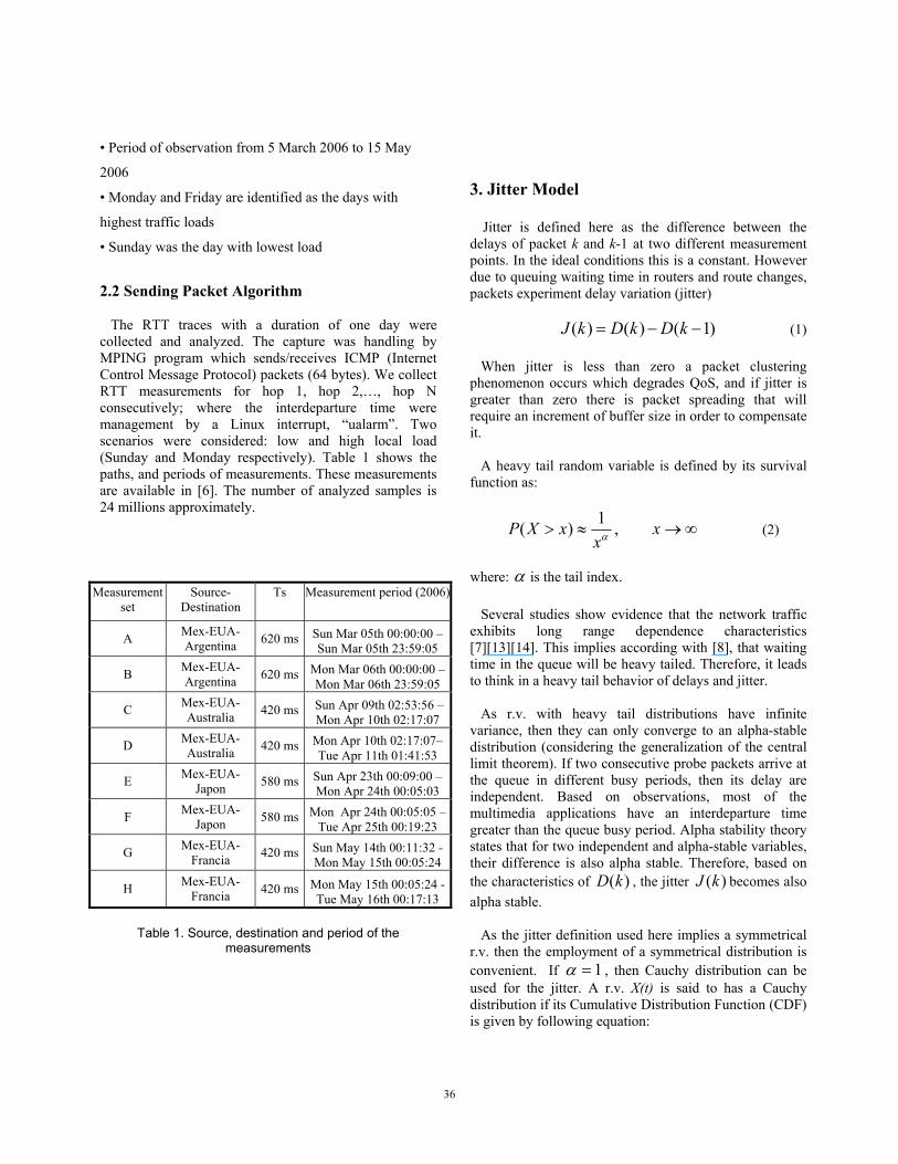
In Figure 2 are shown the estimations of alpha for different methods using 60% of the series length. The smoothing technique showed the best accuracy estimations.

QUANTIL SMOOTHING HILL ALTH

0.4

0.6

0.8

1

1.2

1.4

1.6

Alp

ha E

stim

ated

Method of Estimation Figure 2. Alpha estimated for different methods Figure 3 shows the behavior of α̂ for different hours and router indexes (position in the path).

Figure 3. Alpha behavior in time

Conclusion : The jitter presents a heavy tail distribution. Besides, for the router index > 4, α̂ was close to the unit. Therefore a Cauchy distribution should be taken into account. 3.2 Scale Parameter Estimation According to (3), the scale parameter could be estimated based on its Cumulative Distribution Function (CDF). i.e.

{ }{ }tan ( 1/ 2)x P X xπγ= ≤ − (7)

Also, the equation (7) is a straight line with slope 1/ γ= ; that can be used for γ estimation. 4. Results In the literature, we found only a jitter generator based on Laplace distribution [5]. The Laplace and t-Student distribution are symmetric but some Internet parameters shows heavy tail behavior. Therefore, distribution such as

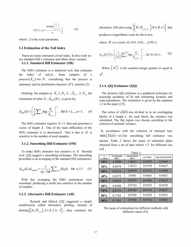
Cauchy should be considered. Figure 4 shows the fit of Cauchy distribution to jitter.

0 0.1 0.2 0.3 0.4 0.5 0.6 0.7 0.8 0.9 10

0.1

0.2

0.3

0.4

0.5

0.6

0.7

0.8

0.9

1

Theoretical

Jitte

r mea

sure

d

P-P plot Jitter set E, 8:00 hrs

ReferenceCauchyLaplacet-Student

Figure 4. P-P of jitter, Cauchy, Laplace and t-Student

distributions The statistic tool of P-P plot compares a theoretical distribution versus a measured distribution (jitter), if they are identical a straight-line with slope 1 is depicted. In order to make a quantitative analysis of the results of P-P plot we calculated the Mean Squared Error (MSE), table 3 shows the results. Conclusion: The Cauchy distribution shows a better fit than Laplace and t-Student for jitter measurements.

Hop Cauchy Laplace t-Student

SET A 1st 5.67E-04 0.0311 0.0899 5th 0.0015 0.0548 0.0327

20th 0.003 0.0295 0.0198

SET B 1st 3.53E-04 0.0263 NaN

06th 0.0015 0.0399 0.0403 23th 0.0019 0.002 0.0368

SET C 1st 4.26E-04 0.0134 NaN

07th 9.31E-04 0.036 0.0436 20th 0.0011 0.0043 0.0016

SET D 1st 4.10E-04 0.0151 NaN

05th 0.0037 0.0057 0.0225 19th 0.0011 0.0035 0.0325

SET E 1st 1.93E-04 0.0374 NaN

10th 0.0061 0.025 0.0144 20th 4.62E-04 0.0309 0.0159

SET F 1st 9.03E-04 0.0157 NaN

07th 0.0016 0.0056 0.0302 21th 0.0024 0.0083 0.0246

SET G 2nd 1.73E-04 0.0426 0.082 12th 4.19E-04 0.0283 0.0492 21th 2.95E-04 0.0247 0.0018

SET H 2nd 2.19E-04 0.0527 0.0808 16th 6.57E-04 0.0042 0.0113 21th 1.91E-04 0.007 0.0533

Table 3. Fitting Mean Squared Error of reference and (t-Student, Cauchy and Laplace) distribution

As the jitter is dominated by queuing in routers, then the higher the number of routers is, the higher the jitter. A

38

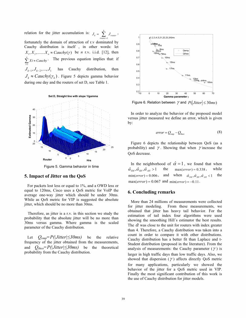
relation for the jitter accumulation is: 1

k

k routerrouter

J J=

= ∑ ,

fortunately the domain of attraction of r.v dominated by Cauchy distribution is itself , in other words: let

1 2, ,....... ( )nX X X Cauchy γ≈ be n r.v. i.i.d. [12], then

1

N

iXi Cauchy

=

≈∑ . The previous equation implies that: if

1 2 1, ,...,k kJ J J− − has Cauchy distribution, then

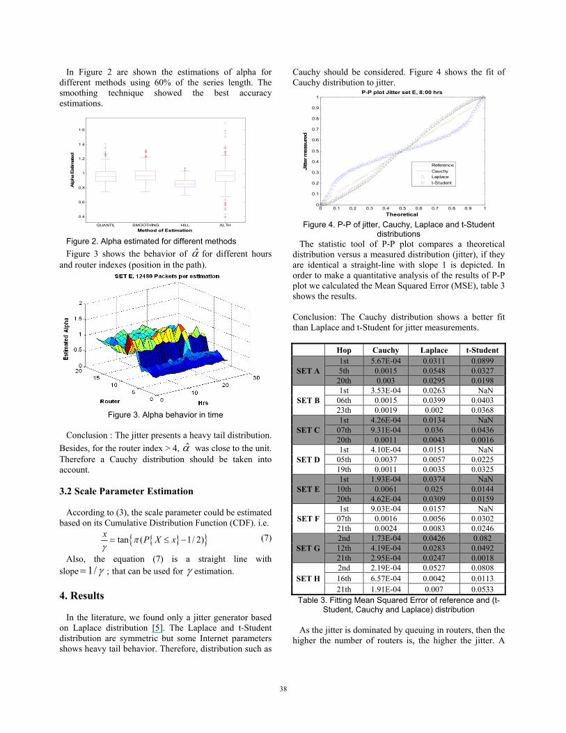
( )k kJ Cauchy γ≈ . Figure 5 depicts gamma behavior during one day and the routers of set D, see Table 1.

05

1015

2025

05

10

15200

10

20

30

40

Hrs

Set D, Straight line with slope 1/gamma

Router

Estim

ated

Gam

ma

Figure 5. Gamma behavior in time

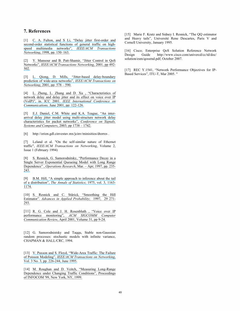
5. Impact of Jitter on the QoS For packets lost less or equal to 1%, and a OWD less or equal to 120ms, Cisco uses a QoS metric for VoIP the average one-way jitter which should be under 30ms. While as QoS metric for VIP is suggested the absolute jitter, which should be no more than 30ms. Therefore, as jitter is a r.v. in this section we study the probability that the absolute jitter will be no more than 30ms versus gamma. Where gamma is the scaled parameter of the Cauchy distribution. Let Qemp=P(|Jitter|≤30ms) be the relative frequency of the jitter obtained from the measurements, and Qtheo=P(|Jitter|≤30ms) be the theoretical probability from the Cauchy distribution.

-10 0 10 20 30 40 50 60 700.2

0.3

0.4

0.5

0.6

0.7

0.8

0.9

1

Gamma parameter γ

(1,2,3,4,5,21,22,23,24)hrs

← 6hrs← 7hrs

← 8hrs

← 9hrs

← 10hrs

← 11hrs

12hrs → ← 13hrs← 14hrs

← 15hrs

← 16hrs

← 17hrs

18hrs →

19hrs →

← 20hrs QempQtheo

Figure 6. Relation between γ and ( 30 )P Jitter ms≤

In order to analyze the behavior of the proposed model versus jitter measured we define an error, which is given by:

emp theoerror Q Q= − (8) Figure 6 depicts the relationship between QoS (as a probability) and γ . Showing that when γ increase the QoS decrease. In the neighborhood of ˆ 1α = , we found that when ˆ ˆ ˆ, , 1SM SH AHα α α > the max( ) 0.338error = , while

min( ) 0.006error = , and when ˆ ˆ ˆ, , 1SM SH AHα α α < the max( ) 0.067error = and min( ) 0.11error = − . 6. Concluding remarks More than 24 millions of measurements were collected for jitter modeling. From these measurements, we obtained that jitter has heavy tail behavior. For the estimation of tail index four algorithms were used showing the smoothing Hill´s estimator the best results. The α̂ was close to the unit for routers with index greater than 4. Therefore, a Cauchy distribution was taken into a count in order to compare it with other distributions. Cauchy distribution has a better fit than Laplace and t-Student distribution (proposed in the literature). From the analysis of measurements: the Cauchy parameter (γ ) is larger in high traffic days than low traffic days. Also, we showed that dispersion (γ ) affects directly QoS metric for many applications, particularly we showed the behavior of the jitter for a QoS metric used in VIP. Finally the most significant contribution of this work is the use of Cauchy distribution for jitter models.

39

7. References [1] C. A. Fulton, and S Li, “Delay jitter first-order and second-order statistical functions of general traffic on high-speed multimedia networks”, IEEE/ACM Transactions Networking, 1998, pp. 150–163. [2] Y. Mansour and B. Patt-Shamir, “Jitter Control in QoS Networks”, IEEE/ACM Transactions Networking, 2001, pp 492-502. [3] L. Qiong, D. Mills, “Jitter-based delay-boundary prediction of wide-area networks”, IEEE/ACM Transactions on Networking, 2001, pp: 578 – 590. [4] L. Zheng, L. Zhang and D. Xu , “Characteristics of network delay and delay jitter and its effect on voice over IP (VoIP)”, in. ICC 2001. IEEE International Conference on Communications, June 2001, pp: 122-126. [5] E.J. Daniel, C.M. White and K.A. Teague, “An inter-arrival delay jitter model using multi-structure network delay characteristics for packet networks”, Conference on Signals, Systems and Computers, 2003; pp 1738 – 1742. [6] http://orion.gdl.cinvestav.mx/jcinv/minisitios/dtorres . [7] Leland et al. "On the self-similar nature of Ethernet traffic", IEEE/ACM Transactions on Networking, Volume 2, Issue 1 (February 1994) [8] S. Resnick, G. Samorodnitsky, “Performance Decay in a Single Server Exponential Queueing Model with Long Range Dependence” , Operations Research, Mar. – Apr; 1997, pp. 235-243. [9] B.M. Hill, “A simple approach to inference about the tail of a distribution”, The Annals of Statistics; 1975, vol. 3, 1163- 1174. [10] S. Resnick and C. Stâricâ, “Smoothing the Hill Estimator”. Advances in Applied Probability; 1997, 29 271-293. [11] R. G. Cole and J. H. Rosenbluth , “Voice over IP performance monitoring”, ACM SIGCOMM Computer Communication Review, April 2001, Volume 31, pp 9-24. [12] G. Samorodnistsky and Taqqu, Stable non-Gaussian random processes: stochastic models with infinite variance, CHAPMAN & HALL/CRC, 1994. [13] V. Paxson and S. Floyd, “Wide-Area Traffic: The Failure of Poisson Modeling”, IEEE/ACM Transactions on Networking, Vol. 3 No. 3, pp. 226-244, June 1995. [14] M. Roughan and D. Veitch, “Measuring Long-Range Dependence under Changing Traffic Conditions”, Proceedings of INFOCOM '99, New York, NY, 1999.

[15] Marie F. Kratz and Sidney I. Resnick, “The QQ estimator and Heavy tails”, Université Rene Descartes, Paris V and Cornell University, January 1995. [16] Cisco; Enterprise QoS Solution Reference Network Design Guide http://www.cisco.com/univercd/cc/td/doc/ solution/esm/qossrnd.pdf; October 2007.

[17] REC Y.1541, “Network Performance Objectives for IP-Based Services”, ITU-T, Mar 2005. "

40