Journal of Functional Analysis 256 (2009) 1642–1664

www.elsevier.com/locate/jfa

A new multilinear insight on Littlewood’s4/3-inequality

Andreas Defant a,1, Pablo Sevilla-Peris a,b,∗,2

a Institute of Mathematics, Carl von Ossietzky University, D-26111 Oldenburg, Germanyb Departamento de Matemática Aplicada and IUMPA, ETSMRE, Universidad Politécnica de Valencia,

Av. Blasco Ibáñez, 21, E-46010 Valencia, Spain

Received 29 May 2008; accepted 3 July 2008

Available online 8 August 2008

Communicated by J. Bourgain

Abstract

We unify Littlewood’s classical 4/3-inequality (a forerunner of Grothendieck’s inequality) together withits m-linear extension due to Bohnenblust and Hille (which originally settled Bohr’s absolute convergenceproblem for Dirichlet series) with a scale of inequalties of Bennett and Carl in �p-spaces (which are of fun-damental importance in the theory of eigenvalue distribution of power compact operators). As an applicationwe give estimates for the monomial coefficients of homogeneous �p-valued polynomials on c0.© 2008 Elsevier Inc. All rights reserved.

Keywords: Multilinear theory; Local Banach space theory; Summing operators

1. Introduction

In 1930 Littlewood settled a long-standing question of Daniell. Motivated through his analysisof Daniell’s problem Littlewood in [30, Theorem 1] proved an inequality nowadays sometimes

* Corresponding author at: Departamento de Matemática Aplicada and IUMPA, ETSMRE, Universidad Politécnica deValencia, Av. Blasco Ibáñez, 21, E-46010 Valencia, Spain.

E-mail addresses: defant@mathematik.uni-oldenburg.de (A. Defant), psevilla@mat.upv.es (P. Sevilla-Peris).1 Supported by the MEC Project MTM2005-08210.2 Supported by the MEC Project MTM2005-08210 and grants PR2007-0384 (MEC) and UPV-PAID-00-07.

0022-1236/$ – see front matter © 2008 Elsevier Inc. All rights reserved.doi:10.1016/j.jfa.2008.07.005

A. Defant, P. Sevilla-Peris / Journal of Functional Analysis 256 (2009) 1642–1664 1643

cited as Littlewood’s 4/3-inequality: for every bilinear form A : c0 × c0 → C (c0 the Banachspace of all scalar zero sequences) the following holds:

( ∞∑i,j=1

∣∣A(ei, ej )∣∣4/3

)3/4

�√

2‖A‖, (1)

and the exponent 4/3 is optimal; here as usual the norm of A is given by

‖A‖ = sup{∣∣A(x1, x2)

∣∣: ‖xi‖∞ � 1}.

In 1931 Bohnenblust and Hille proved [4, Theorem I] that for each m ∈ N and every m-linearmapping A : c0 × · · · × c0 → C the following holds:

( ∞∑i1,...,im=1

∣∣A(ei1, . . . , eim)∣∣ 2m

m+1

)m+12m

� 2m−1

2 ‖A‖, (2)

and showed that the exponent 2mm+1 is optimal. Using this they answered Harald Bohr’s so called

absolute convergence problem for Dirichlet series which had been open for over 15 years (seebelow). Inequality (2) was overlooked for long time and re-discovered by Davie and Kaijser

in [11] and [25] (in fact with the constant 2m−1

2 given in (2) which is better than the original onefrom [4]).

More recently, in [6, Theorem 3.2] the following vector-valued variant was proved. Fix some1 � p � ∞ and m. Then the optimal exponent 1 � r � ∞ for which there is a constant Cp > 0satisfying

( ∞∑i1,...,im=1

∥∥A(ei1, . . . , eim)∥∥r

p

)1/r

� Cmp ‖A‖, (3)

for every m-linear mapping A : c0 × · · · × c0 → �p , is given by

r ={

2 if p � 2,

p if p � 2.

Note that the case m = 1 goes back to Orlicz [33]. In the beginning of the 1970s Bennett [2] andCarl [9] independently proved the following. Define for given 1 � p � q � ∞ the number

r ={

21+2( 1

p−max{ 1

q, 1

2 }) if p � 2,

p if p � 2.

Then there is a constant Cp,q > 0 such that for each linear operator A : c0 → �p we have

( ∞∑∥∥A(ei)∥∥r

q

)1/r

� Cp,q‖A‖. (4)

i=1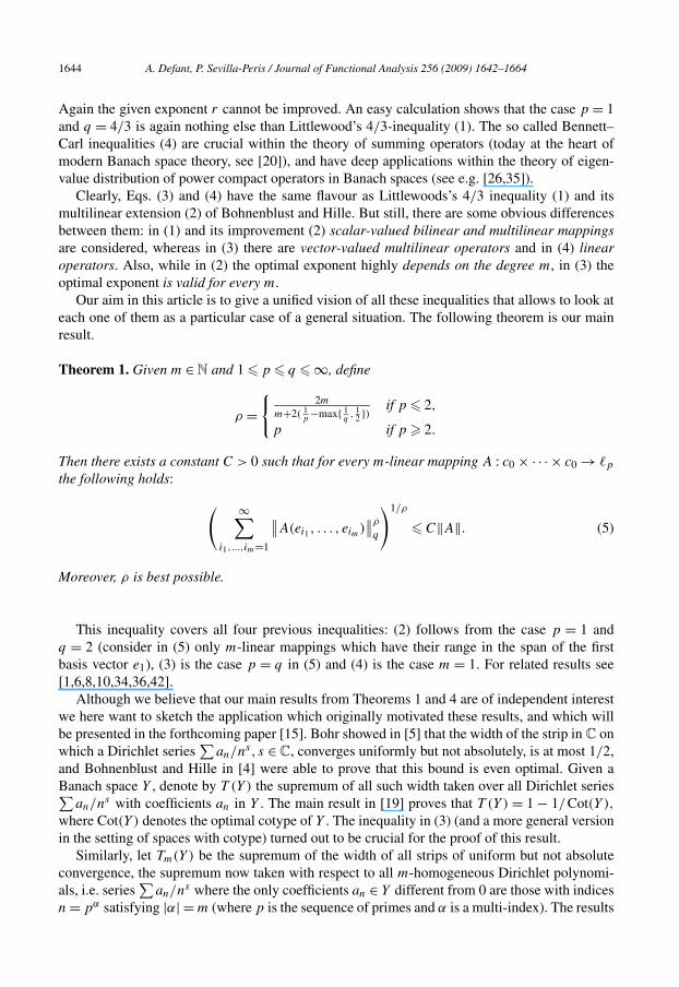

1644 A. Defant, P. Sevilla-Peris / Journal of Functional Analysis 256 (2009) 1642–1664

Again the given exponent r cannot be improved. An easy calculation shows that the case p = 1and q = 4/3 is again nothing else than Littlewood’s 4/3-inequality (1). The so called Bennett–Carl inequalities (4) are crucial within the theory of summing operators (today at the heart ofmodern Banach space theory, see [20]), and have deep applications within the theory of eigen-value distribution of power compact operators in Banach spaces (see e.g. [26,35]).

Clearly, Eqs. (3) and (4) have the same flavour as Littlewoods’s 4/3 inequality (1) and itsmultilinear extension (2) of Bohnenblust and Hille. But still, there are some obvious differencesbetween them: in (1) and its improvement (2) scalar-valued bilinear and multilinear mappingsare considered, whereas in (3) there are vector-valued multilinear operators and in (4) linearoperators. Also, while in (2) the optimal exponent highly depends on the degree m, in (3) theoptimal exponent is valid for every m.

Our aim in this article is to give a unified vision of all these inequalities that allows to look ateach one of them as a particular case of a general situation. The following theorem is our mainresult.

Theorem 1. Given m ∈ N and 1 � p � q � ∞, define

ρ ={

2m

m+2( 1p

−max{ 1q, 1

2 }) if p � 2,

p if p � 2.

Then there exists a constant C > 0 such that for every m-linear mapping A : c0 × · · · × c0 → �p

the following holds:

( ∞∑i1,...,im=1

∥∥A(ei1 , . . . , eim)∥∥ρ

q

)1/ρ

� C‖A‖. (5)

Moreover, ρ is best possible.

This inequality covers all four previous inequalities: (2) follows from the case p = 1 andq = 2 (consider in (5) only m-linear mappings which have their range in the span of the firstbasis vector e1), (3) is the case p = q in (5) and (4) is the case m = 1. For related results see[1,6,8,10,34,36,42].

Although we believe that our main results from Theorems 1 and 4 are of independent interestwe here want to sketch the application which originally motivated these results, and which willbe presented in the forthcoming paper [15]. Bohr showed in [5] that the width of the strip in C onwhich a Dirichlet series

∑an/ns, s ∈ C, converges uniformly but not absolutely, is at most 1/2,

and Bohnenblust and Hille in [4] were able to prove that this bound is even optimal. Given aBanach space Y , denote by T (Y ) the supremum of all such width taken over all Dirichlet series∑

an/ns with coefficients an in Y . The main result in [19] proves that T (Y ) = 1 − 1/Cot(Y ),

where Cot(Y ) denotes the optimal cotype of Y . The inequality in (3) (and a more general versionin the setting of spaces with cotype) turned out to be crucial for the proof of this result.

Similarly, let Tm(Y ) be the supremum of the width of all strips of uniform but not absoluteconvergence, the supremum now taken with respect to all m-homogeneous Dirichlet polynomi-als, i.e. series

∑an/ns where the only coefficients an ∈ Y different from 0 are those with indices

n = pα satisfying |α| = m (where p is the sequence of primes and α is a multi-index). The results

A. Defant, P. Sevilla-Peris / Journal of Functional Analysis 256 (2009) 1642–1664 1645

in [19] as a byproduct show that T (Y ) always equals Tm(Y ) whenever Y is infinite-dimensional.For finite-dimensional Y , however, the situation is drastically different—inequality (18) (a poly-nomial version of (2)) is used in [4] to prove that Tm(C) = m−1

2mwhich as a consequence even

allows to prove that Tm(Y ) = m−12m

whenever dimY < ∞. The question then is

Is it possible to give a unified vision of the formulas Tm(Y ) = 1 − 1/Cot(Y ) (Y infi-nite-dimensional) and Tm(Y ) = m−1

2m(Y finite-dimensional)? Or more vaguely, why do the

m-homogeneous Dirichlet polynomials in infinite-dimensional case disappear?

In the same way as (2) and (3) play an important role in [4,19], so also using Theorem 1 weare able to give a complete answer in the �p-case in [15]: For 1 � p � q � ∞ we consider m-homogeneous Dirichlet polynomials

∑an/ns in �q whose coefficients an ∈ �p and for each one

of them the difference between the abscissa of uniform convergence in �p and that of absoluteconvergence in �q . We then define Tm(p,q) to be the maximal width of these strips in C. Thisnumber somehow measures how much the summability of a homogeneous Dirichlet polynomialin �p improves when we move from �p to a bigger �q . Then

Tm(p,q) ={

m−2(1/p−max{1/q,1/2})2m

if 1 � p � 2,1p′ if 2 � p.

Let us give a brief review of the contain of this article. After some preliminaries given in Sec-tion 1, Section 2 is devoted to the proof of Theorem 1. The main step is Lemma 3, a resultgiven in terms of summing operators and injective tensor product. The optimality of the givenexponent ρ in (5) follows from random techniques. The main result in Section 3 is Theorem 4,a ‘symmetrization’ of Theorem 1 which replaces the m-linear mappings A : c0 ×· · ·×c0 → �p bym-homogeneous polynomials P : c0 → X, and the matrix entries of A by the coefficients cα(P )

in the monomial series expansion∑

α∈N(N)0

cα(P )zα of P . For scalar-valued m-homogeneous

polynomials P : c0 → C, the case p = 1 and q = 2 recovers the important result [4, Section 2]due to Bohnenblust and Hille (see also [37, Theorem III-1]). Finally, in Section 4 we try to inte-grate our study into the theory of summing operators in a more systematic way. We introduce thenotion of (r,1)-summing operators v : X → Y of order m and Bohnenblust–Hille indices. Thisallows us to reformulate some deep facts from local Banach space theory into interesting newLittlewood–Bohnenblust–Hille type inequalities.

2. Preliminaries

Standard notation and notions from Banach space theory are used, as presented e.g. in [28,29].All Banach spaces X are over the real or complex field K, their duals are denoted by X∗ and theiropen unit balls by BX . Given a Banach space X, the space of all sequences (xn) in X such that∑

n ‖xn‖p < ∞ is denoted �p(X). As usual �p(K) = �p and �np = (Kn,‖ ‖p). By a Banach

sequence space we will mean a Banach space X of scalar sequences such that �1 ⊆ X ⊆ �∞satisfying that if x ∈ KN and y ∈ X are such that |x| � |y| then x ∈ X and ‖x‖ � ‖y‖. A Banachsequence space X is symmetric whenever a given scalar sequence x belongs to X if and only if itsdecreasing rearrangement x� does, and in this case they have the same norm. The Banach spaceof all (bounded) linear operators between two Banach spaces X and Y is denoted by L(X,Y ),and the Banach space of all (bounded) m-linear mappings from X × · · · × X to Y by L(mX,Y ).

1646 A. Defant, P. Sevilla-Peris / Journal of Functional Analysis 256 (2009) 1642–1664

We refer to [12] for all needed background on the metric theory of tensor products, and [21,22]for whatever is used on polynomials and symmetric tensor products. Let us recall that the injec-tive norm ‖ · ‖ε of an element z = ∑

k xk ⊗ yk (a fixed finite representation) in the tensor productX ⊗ Y of two Banach spaces is given by

‖z‖ε = sup‖x∗‖X∗ �1‖y∗‖Y∗ �1

∣∣∣∣∑k

x∗(xk)y∗(yk)

∣∣∣∣.

As usual, we write X⊗ε Y for the injective tensor product of X and Y , and⊗m

ε X := X⊗ε · · ·⊗ε

X for the mth full injective tensor product. A function P : X → Y between two Banach spacesis said to be an m-homogeneous polynomial if there is an m-linear mapping ϕ : ∏m

k=1 X → Y

such that P(x) = ϕ(x, . . . , x) for all x ∈ X. We denote by P (mX,Y ) the vector space of allm-homogeneous continuous polynomials P : X → Y which together with the norm ‖P ‖ :=sup‖x‖X�1 ‖P(x)‖Y forms a Banach space. It is well known [21, Proposition 1.8] that the normsof an m-homogeneous polynomial and of the associated m-linear mapping are related in thefollowing way:

‖P ‖ � ‖ϕ‖ � c(m,X)‖P ‖, (6)

where c(m,X) denotes the polarization constant of E [21, Defintion 1.40] that satisfies 1 �c(m,X) � mm

m! .It will be often more convenient to think in terms of symmetric tensor products instead of

spaces of polynomials. We write⊗m,s

εsX for the mth symmetric injective tensor product. Let us

recall that⊗m,s

X can be realized as the range of the symmetrization operator

σm :⊗m

X →⊗m

X, σm(⊗yk) := 1

m!∑

π∈Πm

⊗yπ(k), (7)

where Πm stands for the group of all permutations of {1, . . . ,m}. The following isometric equal-ity will be frequently used: for every finite-dimensional Banach space X and any Banach space Y

⊗m

εX∗ ⊗ε Y = L

(mX,Y

),

(x∗

1 ⊗ · · · ⊗ x∗m

) ⊗ y �[z �

∏k

x∗k (x)y

], (8)

⊗m,s

εs

X∗ ⊗ε Y = P(m

X,Y),

(x∗ ⊗ · · · ⊗ x∗) ⊗ y �

[x � x∗(x)my

]. (9)

For all needed information on the theory of summing operators as well as local Banach spacetheory see [20,40]. Given 1 � p,q � ∞ and some operator v ∈ L(X,Y ), the infimum over allc > 0 such that for each choice of finitely many x1, . . . , xn ∈ X we have

(n∑

i=1

‖vxi‖p

)1/p

� c sup‖x∗‖�1

(n∑

i=1

∣∣x∗(xi)∣∣q)1/q

,

A. Defant, P. Sevilla-Peris / Journal of Functional Analysis 256 (2009) 1642–1664 1647

is called the (p, q)-summing norm of v and denoted πp,q(v). Then v is said to be (p, q)-summing whenever πp,q(v) < ∞. Operators that are (1,1)-summing are usually called sum-ming. Standard arguments easily show that an operator is (r,1)-summing if and only if there is aconstant C > 0 such that for every linear operator A : c0 → X we have

( ∞∑i=1

∥∥vA(ei)∥∥r

)1/r

� C‖A‖, (10)

and πr,1(v) here is the best constant. We will frequently use the following simple reformulationof the summing norm in terms of tensor products, an immediate consequence of (8): for eachoperator v ∈ L(X,Y )

πp,1(v) = ∥∥ id⊗v : �1 ⊗ε X → �p(Y )∥∥ = sup

n

∥∥ id⊗v : �n1 ⊗ε X → �n

p(Y )∥∥. (11)

Finally, we recall another well established notion from local Banach space theory [20, Chap-ter 11]. Let 2 � p < ∞. A Banach space X is said to have cotype p whenever there is someconstant C > 0 such that for each choice of finitely many vectors x1, . . . , xn ∈ X we have

(n∑

i=1

‖xi‖p

)1/p

� C

(∫ ∥∥∥∥∥n∑

i=1

εi(ω)xi

∥∥∥∥∥2

dω

)1/2

,

where εi are independent Bernoulli random variables; as usual, the best such C is denotedby Cp(X). It is well known that �p has cotype max{p,2}.

3. Proof of the main result

The proof is done by induction on the degree m, and clearly the case m = 1 is valid by theBennett–Carl inequality (4). We follow ideas of Kaijser’s re-proof [25] of the Bohnenblust–Hilleresult, and give the proof in terms of summing norms and tensor products.

Note first that by (10) the exponent r given in (4) is the optimal number for which the identityid : �p ↪→ �q is (r,1)-summing, and in fact this was the original context in which this result wasstated.

We start with two lemmas of independent interest.

Lemma 2. Let v : X → Y be an (r,1)-summing operator for some 1 � r < ∞ where Y is acotype 2 space. Then

πr,1(id ⊗ v : �n

1 ⊗εm· · · ⊗ε �n

1 ⊗ε X → �nm

2 (Y ))�

(√2 C2(Y )

)mπr,1(v).

Proof. We proceed by induction. We consider first the case m = 1. Take x1, . . . , xN ∈ �n1 ⊗ε X,

each xk = ∑ni=1 ei ⊗ xk(i) where xk(i) ∈ X. We want

(N∑

‖vxk‖r�n

2(Y )

)1/r

�√

2 C2(Y ) supγ∈B(�n⊗ X)∗

N∑∣∣γ (xk)∣∣, (12)

k=1 1 ε k=1

1648 A. Defant, P. Sevilla-Peris / Journal of Functional Analysis 256 (2009) 1642–1664

and start dealing with the left-hand side of this inequality. Applying first that Y has cotype 2,second the well-known fact that (

∫ ‖∑i xiεi(ω)‖2 dω)1/2 �

√2∫ ‖∑

i xiεi(ω)‖dω (see e.g.[20, Theorem 11.1 and p. 227]), then the (continuous) Minkowski inequality and last that v is(r,1)-summing we get

(N∑

k=1

‖vxk‖r�n

2(Y )

)1/r

=(

N∑k=1

((n∑

i=1

∥∥vxk(i)∥∥2

Y

)1/2)r)1/r

�√

2 C2(Y )

(N∑

k=1

(∫ ∥∥∥∥∥n∑

i=1

vxk(i)εi(ω)

∥∥∥∥∥Y

dω

)r)1/r

�√

2 C2(Y )

∫ (N∑

k=1

∥∥∥∥∥n∑

i=1

vxk(i)εi(ω)

∥∥∥∥∥r

Y

)1/r

dω

�√

2 C2(Y )πr,1(v)

∫sup

x∗∈BX∗

N∑k=1

∣∣∣∣∣x∗(

n∑i=1

xk(i)εi(ω)

)∣∣∣∣∣dω

�√

2 C2(Y )πr,1(v) supλ∈B

�N∞

supη∈B�n∞

∥∥∥∥∥N∑

k=1

n∑i=1

xk(i)η(i)λk

∥∥∥∥∥X

.

On the other hand, we have, for the right-hand side of the inequality (12),

supγ∈B(�n1⊗εX)∗

N∑k=1

∣∣γ (xk)∣∣ = sup

λ∈B�N∞

∥∥∥∥∥N∑

k=1

xkλk

∥∥∥∥∥�n

1⊗εX

= supλ∈B

�N∞

supη∈B

�n∞x∗∈BX∗

∣∣∣∣∣n∑

i=1

N∑k=1

η(i)x∗(xk(i))λk

∣∣∣∣∣

= supλ,η

supx∗∈BX∗

∣∣∣∣∣x∗(

n∑i=1

N∑k=1

η(i)xk(i)λk

)∣∣∣∣∣= sup

λ,η

∥∥∥∥∥N∑

k=1

n∑i=1

xk(i)η(i)λk

∥∥∥∥∥X

.

This shows that

πr,1(id ⊗ v : �n

1 ⊗ε X → �n2(Y )

)�

√2 C2(Y )πr,1(v). (13)

Let us assume that

πr,1(id ⊗ v : �n ⊗ε

m−1· · · ⊗ε �n ⊗ε X → �nm−1(Y )

)�

(√2 C2(Y )

)m−1πr,1(v).

1 1 2

A. Defant, P. Sevilla-Peris / Journal of Functional Analysis 256 (2009) 1642–1664 1649

Define V = �n1 ⊗ε

m−1· · · ⊗ε �n1 ⊗ε X, U = �nm−1

2 (Y ) and w = id⊗v : V → U . It is easily seen

that �nm−1

2 (Y ) has cotype 2 with C2(�nm−1

2 (Y )) � C2(Y ). Then by (13)

πr,1(id ⊗ w : �n

1 ⊗ε V → �n2(U)

)�

√2 C2

(�nm−1

2 (Y ))πr,1(w)

�√

2 C2(Y )(√

2 C2(Y ))m−1

πr,1(v),

which completes the proof. �The second lemma is based on complex interpolation and will handle the case p � 2 in (5).

Lemma 3. Let m ∈ N, Y a Banach space with cotype 2, and v : X → Y an (r,1)-summingoperator with 1 � r � 2. Define

ρ = 2m

m + 2(1/r − 1/2).

Then there is some C > 0 such that for every m-linear mapping A : c0 × · · · × c0 → X thefollowing holds

( ∞∑i1,...,im=1

∥∥vA(ei1, . . . , eim)∥∥ρ

Y

)1/ρ

� C‖A‖.

Let us note that our proof shows C � (√

2 C2(Y ))m−1πr,1(v).

Proof. By (8) we have to show that there exists some constant C > 0 such that, for all n,

∥∥id ⊗ v : �n1 ⊗ε

m· · · ⊗ε �n1 ⊗ε X → �nm

ρ (Y )∥∥ � C.

The case m = 1 is simply the fact that v is (r,1)-summing.First, we only consider the case m = 2 (here our proof appears to be a bit more transparent

than in the general argument given later).On one hand, we have from Lemma 2 that

πr,1(id ⊗ v : �n

1 ⊗ε X → �n2(Y )

)�

√2 C2(Y )πr,1(v),

hence by (11)

∥∥id ⊗ v : �n1 ⊗ε �n

1 ⊗ε X → �nr

(�n

2(Y ))∥∥ �

√2 C2(Y )πr,1(v). (14)

Given 1 � s � 2 and elements y(k, l) ∈ Y with k = 1, . . . ,M and l = 1, . . . ,N , we have byMinkowski’s inequality that

1650 A. Defant, P. Sevilla-Peris / Journal of Functional Analysis 256 (2009) 1642–1664

(N∑

l=1

∥∥y(·, l)∥∥2�Ms (Y )

)1/2

=(

N∑l=1

(M∑

k=1

∥∥y(k, l)∥∥s

Y

)2/s)1/2

�(

M∑k=1

(N∑

l=1

∥∥Y(k, l)∥∥2

Y

)2/s)1/s

=(

M∑k=1

∥∥y(k, ·)∥∥s

�M2 (Y )

)1/s

.

This shows that the operator

T : �Ms

(�N

2 (Y )) → �N

2

(�Ms (Y )

),

((y(k, l)

)N

l=1

)M

k=1 �((

y(k, l))M

k=1

)N

l=1

has norm � 1.On the other hand, we can consider the operator

S : �n1 ⊗ε �n

1 → �n1 ⊗ε �n

1, S(ei ⊗ ej ) = ej ⊗ ei .

Clearly ‖S‖ = 1, and by composition we obtain from (14)

∥∥id ⊗ v : �n1 ⊗ε �n

1 ⊗ε XS⊗idX−−−−→ �n

1 ⊗ε �n1 ⊗ε X

id⊗v−−−→ �nr

(�n

2(Y ))

T−→ �n2

(�nr (Y )

)∥∥�

√2 C2(Y )πr,1(v). (15)

Now we interpolate (14) and (15) with the complex method and θ = 1/2 (see e.g. [3, Chapter 5])and get

∥∥id ⊗ v : �n1 ⊗ε �n

1 ⊗ε X → [�nr

(�n

2(Y )), �n

2

(�nr (Y )

)]1/2

∥∥ �√

2 C2(Y )πr,1(v).

But

[�nr

(�n

2(Y )), �n

2

(�nr (Y )

)]1/2 = [

�nr , �

n2

]1/2

([�n

2, �nr

]1/2(Y )

) = �nμ

(�nν(Y )

),

where 1μ

= 1/2r

+ 1/22 and 1

ν= 1/2

2 + 1/2r

, which finally as desired gives

∥∥id ⊗ v : �n1 ⊗ε �n

1 ⊗ε X → �n2

4r2+r

(Y )∥∥ �

√2 C2(Y )πr,1(v).

We proceed now by induction on m and use the notation ρ = ρm,r . Let us assume that the resultis true for m − 1. From Lemma 2 we have

πr,1(id ⊗ v : �n

1 ⊗εm−1· · · ⊗ε �n

1 ⊗ε X → �nm−1

2 (Y ))�

(√2 C2(Y )

)m−1πr,1(v),

hence

∥∥id ⊗ v : �n1 ⊗ε

m· · · ⊗ε �n1 ⊗ε X → �n

r

(�nm−1

2 (Y ))∥∥ �

(√2 C2(Y )

)m−1πr,1(v). (16)

On the other hand, we consider the operator

A. Defant, P. Sevilla-Peris / Journal of Functional Analysis 256 (2009) 1642–1664 1651

S :�n1 ⊗ε

(�n

1 ⊗εm−1· · · ⊗ε �n

1

) → (�n

1 ⊗εm−1· · · ⊗ε �n

1

) ⊗ε �n1

ei1 ⊗ (ei2 ⊗ · · · ⊗ eim) � (ei2 ⊗ · · · ⊗ eim) ⊗ ei1 .

Again ‖S‖ = 1 and we compose

�n1 ⊗ε

(�n

1 ⊗εm−1· · · ⊗ε �n

1

) ⊗ε X

(S⊗idX)

(�n

1 ⊗εm−1· · · ⊗ε �n

1

) ⊗ε �n1 ⊗ε X

induction

�nm−1

ρm−1,r

(�n

2(Y ))

T

�n2

(�nm−1

ρm−1,r(Y )

),

to get

∥∥id ⊗ v : �n1 ⊗ε

m· · · ⊗ε �n1 ⊗ε X → �n

2

(�nm−1

ρm−1,r(Y )

)∥∥ �(√

2 C2(Y ))m−1

πp,1(v). (17)

Complex interpolation of (16) and (17) with θ = 1/m gives

∥∥id ⊗ v : �n1 ⊗ε

m· · · ⊗ε �n1 ⊗ε X → [

�nr

(�nm−1

2 (Y )), �n

2

(�nm−1

ρm−1,r(Y )

)]1/m

∥∥�

(√2 C2(Y )

)m−1πp,1(v).

But again

[�nr

(�nm−1

2 (Y )), �n

2

(�nm−1

ρm−1,r(Y )

)]1/m

= [�nr , �

n2

]1/m

([�nm−1

2 , �nm−1

ρm−1,r

]1/m

(Y )) = �n

μ

(�nm−1

ν (Y )),

where

1

μ= 1/m

r+ 1 − 1/m

2and

1

ν= 1/m

2+ 1 − 1/m

ρm−1,r

.

This completes the proof. �We can finally give the proof of Theorem 1. Three different cases are considered.

1652 A. Defant, P. Sevilla-Peris / Journal of Functional Analysis 256 (2009) 1642–1664

3.1. The case 1 � p � q � 2

We know from the Bennett–Carl inequalities (4) that the embedding id : �p ↪→ �q is (r,1)-summing, where 1/r = 1/p − 1/q − 1/2. Using this in Lemma 3 together with the fact that �q

for q � 2 has cotype 2, we get (5). In order to see optimality, we assume that r is such that

supn

∥∥ id : �n1 ⊗ε · · · ⊗ε �n

1 ⊗ε �np → �nm

r

(�nq

)∥∥ = c < ∞

(see again (8)). We take families of independent standard Gaussian random variables (gi1,...,im+1),(gi1,...,im) and (gk). By Chevét’s inequalities (see e.g. [40, (43.2)] for the bilinear version and [16,Lemma 6] for the m-linear version) we have for all n

∫ ∥∥∥∥ ∑i1,...,im+1

gi1,...,im+1(ω) ei1 ⊗ · · · ⊗ eim ⊗ eim+1

∥∥∥∥�n

1⊗ε ···⊗ε�n1⊗ε�n

p

dω

� C1

(∫ ∥∥∥∥ ∑i1,...,im

gi1,...,im(ω)ei1 ⊗ · · · ⊗ eim

∥∥∥∥�n

1⊗ε ···⊗ε �n1

dω∥∥ id : �n

2 → �np

∥∥

+ ∥∥ id : �nm

2 → ⊗εm�n

1

∥∥∫ ∥∥∥∥∑k

gkek

∥∥∥∥�np

dω

).

First of all, using [16, Lemma 6] we have

∫ ∥∥∥∥ ∑i1,...,im

gi1,...,im(ω)ei1 ⊗ · · · ⊗ eim

∥∥∥∥�n

1⊗ε ···⊗ε �n1

dω

� K

∫ ∥∥∥∥∑k

gkek

∥∥∥∥�n

1

dω∥∥ id : �n

2 → �n1

∥∥m−1.

Now, it is known (see e.g. [17, (4)]) that∫ ‖∑

k gkek‖�npdω � κn1/p for all 1 � p < ∞. On

the other hand, ‖ id : �nm

2 → ⊗mε �n

1‖ = ‖ id : �n2 → �n

1‖m and ‖ id : �n2 → �n

p‖ = n1/p−1/2 for all1 � p � 1. This altogether gives

∫ ∥∥∥∥ ∑i1,...,im+1

gi1,...,im+1(ω) ei1 ⊗ · · · ⊗ eim ⊗ eim+1

∥∥∥∥�n

1⊗ε ···⊗ε�n1⊗ε�n

p

dω

� C2(n · n(m−1)/2 · n1/p−1/2 + nm/2+1/p

)� C3n

m/2+1/p.

Now it is a well-known fact that the Bernoulli averages are dominated by the Gaussian averages(see e.g. [20, 12.11]). Hence there is some C > 0 such that for all n

∫ ∥∥∥∥ ∑εi1,...,im+1(ω)ei1 ⊗ · · · ⊗ eim ⊗ eim+1

∥∥∥∥�n⊗ε ···⊗ε �n⊗ε�n

p

dω � Cnm/2+1/p,

i1,...,im+1 1 1

A. Defant, P. Sevilla-Peris / Journal of Functional Analysis 256 (2009) 1642–1664 1653

which means that for each n there exists a choice of signs εi1,...,im+1 = ±1 such that

∥∥∥∥zn :=∑

i1,...,im+1

εi1,...,im+1ei1 ⊗ · · · ⊗ eim ⊗ eim+1

∥∥∥∥�n

1⊗ε ···⊗ε �n1⊗ε�n

p

� Cnm/2+1/p.

By our assumption we for all n have

‖zn‖�nmr (�n

q ) � c‖zn‖�n1⊗ε ···⊗ε �n

1⊗ε�np

� cCnm/2+1/p.

But, on the other hand,

‖zn‖�nmr (�n

q ) =∥∥∥∥ ∑

i1,...,im

ei1 ⊗ · · · ⊗ eim ⊗( ∑

im+1

εi1,...,im+1eim+1

)∥∥∥∥�nmr (�n

q )

=( ∑

i1,...,im

∥∥∥∥ ∑im+1

εi1,...,im+1eim+1

∥∥∥∥r

�nq

)1/r

= (nm · nr/q

)1/r.

All in all, we conclude that there is some D > 0 such that for all n

(nm · nr/q

)1/r � Dnm/2+1/p,

which implies the desired inequality m/r + 1/q � m/2 + 1/p.

3.2. The case 1 � p < 2 < q � ∞

We first factor id : �p ↪→ �q through �2. By (4) we know that id : �p ↪→ �2 is (p,1)-summing.We can then apply Lemma 3 combined with ‖ · ‖q � ‖ · ‖2, in order to get the inequality in (5).

The fact that the exponent ρ is best possible now will follow by a careful analysis of tech-niques developed in [4, Section 2]. Without loss of generality we may assume that q = ∞ sinceall exponents satisfying (5) in the case 1 � p < 2 < q � ∞ will also do this in the case 1 � p < 2and q = ∞.

Let r be an exponent satisfying (5) for 1 � p < 2 and q = ∞. Fix n and consider an n × n

matrix (ajk)j,k satisfying

n∑t=1

ajtakt = nδjk and |ajk| = 1 for all j, k

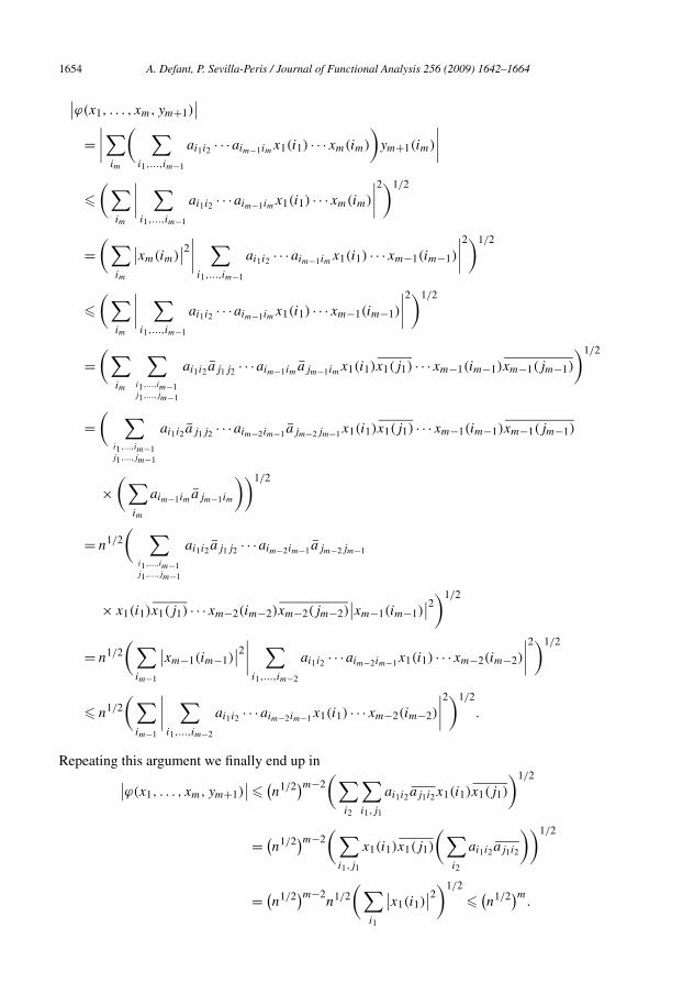
(take, e.g. ajk = e2πi(j−k)/n). With this we define ϕ : �n∞ × m· · · × �n∞ × �n2 → C by

ϕ(x1, . . . , xm, ym+1) =n∑

i1,...,im=1

ai1i2 · · ·aim−1imx1(i1) · · ·xm(im)ym+1(im).

Let us see that ‖ϕ‖ � nm/2; indeed, if x1, . . . , xm ∈ B�n∞ and ym+1 ∈ B�n2

then, using the Cauchy–Schwarz inequality and the first condition of the matrix (ajk)j,k we have

1654 A. Defant, P. Sevilla-Peris / Journal of Functional Analysis 256 (2009) 1642–1664

∣∣ϕ(x1, . . . , xm, ym+1)∣∣

=∣∣∣∣∑

im

( ∑i1,...,im−1

ai1i2 · · ·aim−1imx1(i1) · · ·xm(im)

)ym+1(im)

∣∣∣∣�

(∑im

∣∣∣∣ ∑i1,...,im−1

ai1i2 · · ·aim−1imx1(i1) · · ·xm(im)

∣∣∣∣2)1/2

=(∑

im

∣∣xm(im)∣∣2

∣∣∣∣ ∑i1,...,im−1

ai1i2 · · ·aim−1imx1(i1) · · ·xm−1(im−1)

∣∣∣∣2)1/2

�(∑

im

∣∣∣∣ ∑i1,...,im−1

ai1i2 · · ·aim−1imx1(i1) · · ·xm−1(im−1)

∣∣∣∣2)1/2

=(∑

im

∑i1,...,im−1j1,...,jm−1

ai1i2aj1j2 · · ·aim−1imajm−1imx1(i1)x1(j1) · · ·xm−1(im−1)xm−1(jm−1)

)1/2

=( ∑

i1,...,im−1j1,...,jm−1

ai1i2aj1j2 · · ·aim−2im−1ajm−2jm−1x1(i1)x1(j1) · · ·xm−1(im−1)xm−1(jm−1)

×(∑

im

aim−1imajm−1im

))1/2

= n1/2( ∑

i1,...,im−1j1,...,jm−1

ai1i2aj1j2 · · ·aim−2im−1ajm−2jm−1

× x1(i1)x1(j1) · · ·xm−2(im−2)xm−2(jm−2)∣∣xm−1(im−1)

∣∣2)1/2

= n1/2( ∑

im−1

∣∣xm−1(im−1)∣∣2

∣∣∣∣ ∑i1,...,im−2

ai1i2 · · ·aim−2im−1x1(i1) · · ·xm−2(im−2)

∣∣∣∣2)1/2

� n1/2( ∑

im−1

∣∣∣∣ ∑i1,...,im−2

ai1i2 · · ·aim−2im−1x1(i1) · · ·xm−2(im−2)

∣∣∣∣2)1/2

.

Repeating this argument we finally end up in∣∣ϕ(x1, . . . , xm, ym+1)∣∣ �

(n1/2)m−2

(∑i2

∑i1,j1

ai1i2aj1i2x1(i1)x1(j1)

)1/2

= (n1/2)m−2

( ∑i1,j1

x1(i1)x1(j1)

(∑i2

ai1i2aj1i2

))1/2

= (n1/2)m−2

n1/2(∑∣∣x1(i1)

∣∣2)1/2

�(n1/2)m

.

i1

A. Defant, P. Sevilla-Peris / Journal of Functional Analysis 256 (2009) 1642–1664 1655

This ϕ induces an m-linear mapping ϕ : �n∞ × · · · × �n∞ → �n2 with ‖ϕ‖ = ‖ϕ‖. Composing with

the inclusion we define an m-linear mapping

A : �n∞ × · · · × �n∞ → �n2 ↪→ �n

p

with norm ‖A‖ � ‖ϕ‖ ‖ id : �n2 ↪→ �n

p‖ � nm/2n1/p−1/2. Then by our assumption on r ,

( n∑i1,...,im=1

∥∥A(ei1, . . . , eim)∥∥r

∞

)1/r

� Cmnm/2n1/p−1/2.

Let us compute now the left-hand side. Each A(ei1, . . . , eim) is a vector in �np whose kth compo-

nent is given by

A(ei1, . . . , eim)(k) = ϕ(ei1, . . . , eim, ek)

=n∑

j1,...,jm=1

aj1j2 · · ·ajm−1jmei1(j1) · · · eim(jm)ek(jm),

and this is ai1i2 · · ·aim−1im if im = k and 0, otherwise. Hence A(ei1, . . . , eim) has all its entriesbut the imth equal to 0. Then ‖A(ei1, . . . , eim)‖∞ = 1 (since |ajk| = 1 for all j, k) and we havenm/r � Cmnm/2n1/p−1/2 for every n. This gives as desired

r � 2m

m + 2( 1p

− 12 )

.

3.3. The case 2 � p � q � ∞

We have by (3) that if A ∈ L(m�n∞, �p) then

( ∑i1,...,im

‖ai1,...,im‖pq

)1/p

�( ∑

i1,...,im

‖ai1,...,im‖pp

)1/p

� Cmp ‖A‖,

i.e. for each m the exponent ρ = p satisfies (5). Assume conversely that the exponent r sat-isfies (5) for m. Then an easy argument shows that r satisfies (5) for m = 1, in other terms:id : �p ↪→ �q is (r,1)-summing. From the optimality in the Bennett–Carl inequalities (4) we getthat r � p.

This completes the proof of Theorem 1. �4. Bohnenblust–Hille type results for polynomials

Every m-homogeneous polynomial P defined on a Banach sequence space X with valuesin some Banach space Y has a monomial series expansion

∑α∈N

n0c(n)α (P )zα whenever it is

restricted to any finite-dimensional section Xn (the span of the first n basis vectors ei ) of X.

1656 A. Defant, P. Sevilla-Peris / Journal of Functional Analysis 256 (2009) 1642–1664

And clearly we have c(n)α (P ) = c

(n+1)α (P ) for α ∈ N

n0 ⊂ N

n+10 . Thus there is a unique family

(cα(P ))α∈N

(N)0

in Y such that for all n ∈ N and all z ∈ Xn

P (z) =∑

α∈N(N)0

cα(P )zα.

The power series∑

α cα(P )zα is called the monomial expansion of P , and cα = cα(P ) are itsmonomial coefficients.

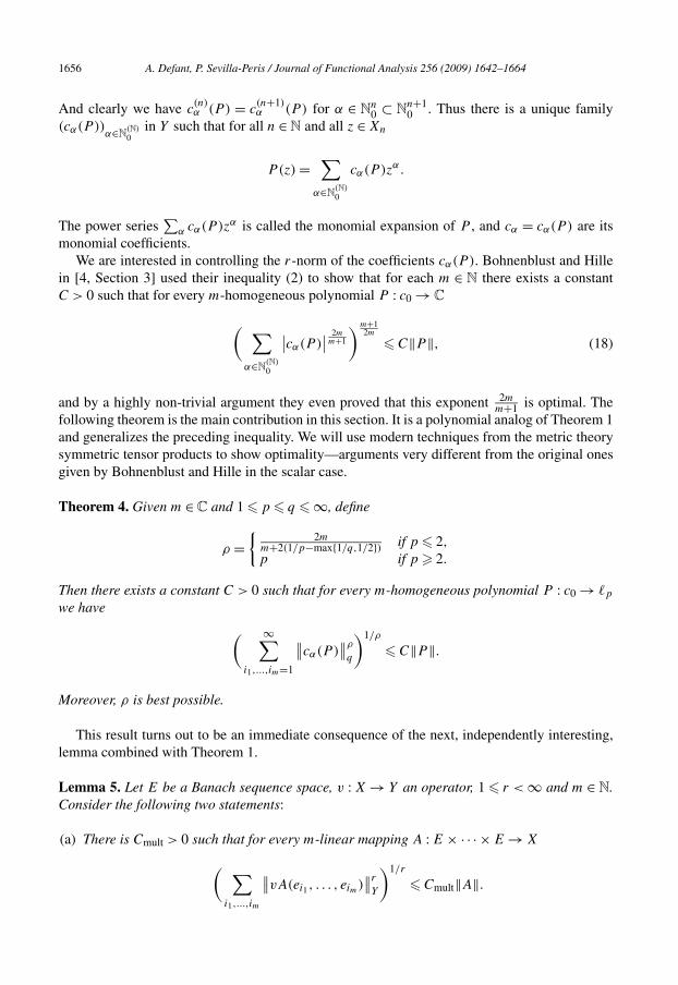
We are interested in controlling the r-norm of the coefficients cα(P ). Bohnenblust and Hillein [4, Section 3] used their inequality (2) to show that for each m ∈ N there exists a constantC > 0 such that for every m-homogeneous polynomial P : c0 → C

( ∑α∈N

(N)0

∣∣cα(P )∣∣ 2m

m+1

)m+12m

� C‖P ‖, (18)

and by a highly non-trivial argument they even proved that this exponent 2mm+1 is optimal. The

following theorem is the main contribution in this section. It is a polynomial analog of Theorem 1and generalizes the preceding inequality. We will use modern techniques from the metric theorysymmetric tensor products to show optimality—arguments very different from the original onesgiven by Bohnenblust and Hille in the scalar case.

Theorem 4. Given m ∈ C and 1 � p � q � ∞, define

ρ ={

2mm+2(1/p−max{1/q,1/2}) if p � 2,

p if p � 2.

Then there exists a constant C > 0 such that for every m-homogeneous polynomial P : c0 → �p

we have

( ∞∑i1,...,im=1

∥∥cα(P )∥∥ρ

q

)1/ρ

� C‖P ‖.

Moreover, ρ is best possible.

This result turns out to be an immediate consequence of the next, independently interesting,lemma combined with Theorem 1.

Lemma 5. Let E be a Banach sequence space, v : X → Y an operator, 1 � r < ∞ and m ∈ N.Consider the following two statements:

(a) There is Cmult > 0 such that for every m-linear mapping A : E × · · · × E → X

( ∑i1,...,im

∥∥vA(ei1, . . . , eim)∥∥r

Y

)1/r

� Cmult‖A‖.

A. Defant, P. Sevilla-Peris / Journal of Functional Analysis 256 (2009) 1642–1664 1657

(b) There is Cpol > 0 such that for every m-homogeneous polynomial P : E → X( ∑|α|=m

∥∥vcα(P )∥∥r

Y

)1/r

� Cpol‖P ‖.

Then (a) always implies (b) with Cpol � (m!)1−1/rc(m,E)Cmult. Conversely, if E is symmetric,then (b) implies (a) with Cmult � m!Cpol.

Proof. We first show that (a) implies (b). Following [16, Section 2] (see also [18, Section 3])we consider the following three index sets:

M(m,n) = {1, . . . , n}m,

J (m,n) = {i = (i1, . . . , im) ∈ M(m,n): i1 � · · · � im

},

Λ(m,n) = {α ∈ N

n0: |α| = m

}.

In M(m,n) we define the following equivalence relation: i ∼ j if there is a permutation π ∈ Πm

such that ik = jπ(k) for all k = 1, . . . ,m. Clearly, the equivalence class of a given index [i] hasat most |Πm| = m! elements; also M(m,n) = ⋃

i∈J (m,n)[i]. Moreover, there is a one-to-onecorrespondence between J (m,n) and Λ(m,n) defined in the following terms. If i ∈ J (m,n)

there is an associated multi-index αi given by αr = |{k: ik = r}| (i.e. α1 is the number of 1’s

in i, α2 is the number of 2’s, . . . ). If α ∈ Λ(m,n) then we define iα = (1,α1· · · ,1,2,

α2· · · ,2, . . . ,

nαn· · · , n) ∈ J (m,n). Note that card[iα] = m!/α!.Let now P : En → X be an m-homogeneous polynomial (where En denotes the span of

the first n basis vectors ek in E), and A : En × · · · × En → X its associated symmetric m-linear mapping. We show now that the monomial coefficients cα(P ) of P and the coefficientsai1,...,im = A(ei1, . . . , eim) defining A are related in the following way:

cα = 1

card[iα]aiα ; (19)

indeed, ∑i∈M(m,n)

ai1,...,imzi1 · · · zim =∑

i∈J (m,n)

∑j∈[i]

ajzj =∑

i∈J (m,n)

card[i]aizi

=∑

α∈Λ(m,n)

card[iα]cαzα.

Then, since 1 � card[iα] � m!, we have( ∑|α|=m

∥∥vcα(P )∥∥r

)1/r

= (m!)1−1/r

( ∑|α|=m

‖vcα(P )‖r

(m!)(1−1/r)r

)1/r

= (m!)1−1/r

( ∑|α|=m

‖vcα(P )‖r

(m!)r−1

)1/r

� (m!)1−1/r

( ∑ ‖vcα(P )‖r

(card[iα])r−1

)1/r

|α|=m

1658 A. Defant, P. Sevilla-Peris / Journal of Functional Analysis 256 (2009) 1642–1664

and hence by (6) and (19)

( ∑|α|=m

∥∥vcα(P )∥∥r

)1/r

� (m!)1−1/r

( ∑|α|=m

card[iα]∥∥∥∥ vcα(P )

card[iα]∥∥∥∥

r)1/r

= (m!)1−1/r

( ∑|α|=m

card[iα]∥∥∥∥ vcα(P )

card[iα]∥∥∥∥

r)1/r

= (m!)1−1/r

( ∑|α|=m

∥∥vA(ei1, . . . , eim)∥∥r

)1/r

� (m!)1−1/rCmult‖A‖ � (m!)1−1/rCmultc(m,E)‖P ‖.

For the proof of the second statement we assume that the Banach sequence space E is symmetric,and deduce from our assumption (b) by (9) that

supn

∥∥∥id ⊗ v :⊗m,s

εs

E∗n ⊗ε X → �d(m,n)

r (Y )

∥∥∥ � Cpol, (20)

here d(m,n) = dim⊗m,s

r �nr = card J (m,n) = ( m+n−1

n−1 ). We will use a technique that was firstconsidered in [7,13], later used in [16,17,23] and finally presented in its more general formin [14]. For each fixed n ∈ N and every i = 1, . . . ,m we consider mappings

Ii : Cn → C

mn Pi : Cmn → C

n

n∑j=1

λjej �n∑

j=1

λjen(i−1)+j

mn∑j=1

λjej �n∑

j=1

λn(i−1)+j ej .

On the other hand, there are the natural embedding and projection (see (7))

ιm :⊗m,s

Cmn →

⊗mC

mn and σm :⊗m

Cmn →

⊗m,sC

mn.

From all this it can be easily deduced that the following diagram is commutative (see [22]):

⊗mC

n⊗m

Cn

⊗mC

mn⊗m

Cmn

⊗m,sC

mn⊗m,s

Cmn�

�

�

�

�

�

⊗m idn

I1⊗···⊗Im m!P1⊗···⊗Pm

σm ιm

⊗m,s idmn

(21)

A. Defant, P. Sevilla-Peris / Journal of Functional Analysis 256 (2009) 1642–1664 1659

Define, for any 1 � r � ∞ and any natural number N , on⊗m,s

r �Nr ⊗ Y the norm induced by

�d(m,N)r (Y ), and denote the resulting Banach space by

⊗m,s

r�Nr ⊗r Y = �d(m,N)

r (Y ).

Tensorizing and putting appropriate norms we obtain in (21):

⊗mε E∗

n ⊗ε X⊗m

r �nr ⊗r Y

⊗mε E∗

mn ⊗ε X⊗m

r �mnr ⊗r Y

⊗m,sεs

E∗mn ⊗ε X

⊗m,sr �mn

r ⊗r Y�

�

�

�

�

�

⊗m id⊗v

I1⊗···⊗Im⊗idX m!P1⊗···⊗Pm⊗idY

σm⊗idX ιm⊗idY

⊗m,s id⊗v

(22)

We now conclude from the metric mapping property of the injective norm, our assumption from(20), the fact that E is symmetric and the very definitions that

∥∥∥I1 ⊗ · · · ⊗ Im ⊗ idX :⊗m

εE∗

n ⊗ε X →⊗m

εE∗

mn ⊗ε X

∥∥∥ � 1,∥∥∥σm ⊗ idX :⊗m

εE∗

mn ⊗ε X →⊗m,s

εs

E∗mn ⊗ε X

∥∥∥ � 1,∥∥∥id ⊗ v :⊗m,s

εs

E∗mn ⊗ε X → �d(m,mn)

r (Y )

∥∥∥ � Cpol,∥∥ιm ⊗ idY : �d(m,mn)r (Y ) → �(mn)m

r (Y )∥∥ � 1,∥∥m!P1 ⊗ · · · ⊗ Pm ⊗ idY : �(mn)m

r (Y ) → �nm

r (Y )∥∥ � m!.

Hence we finally deduce from (22) that

supn

∥∥id ⊗ v :⊗m

εEn ⊗ε X → �nm

r (Y )∥∥ � m!Cpol,

which by (8) finishes the proof. �For E = c0, m ∈ N and v = idC let now Cmult and Cpol be the optimal constants in (a) and (b),

respectively. Then we know that the optimal exponent in (a) is 2mm+1 and Cmult � 2

m−12 . Moreover,

by Harris [24] (see also [32,41]) we have

c(m,E) � mm/2(m + 1)(m+1)/2

,

2mm!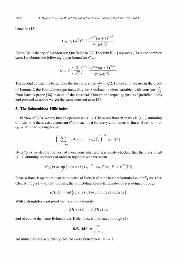

1660 A. Defant, P. Sevilla-Peris / Journal of Functional Analysis 256 (2009) 1642–1664

hence in (18)

Cpol � (√

2)m−1 mm/2(m + 1)m+1

2

2m(m!)m+12m

.

Using Blei’s theory of p-Sidon sets Queffélec in [37, Theorem III-1] reproves (18) in the complexcase. He obtains the following upper bound for Cpol:

Cpol �(

2√π

)m−1mm/2(m + 1)

m+12

2m(m!)m+12m

.

The second constant is better than the first one, since 2√π

<√

2. However, if we use in the proof

of Lemma 2 the Khintchine-type inequality for Steinhaus random variables with constant 2√π

from Sawa’s paper [38] instead of the classical Khintchine inequality (just as Queffélec does)and proceed as above we get the same constant as in [37].

5. The Bohnenblust–Hille index

In view of (10), we say that an operator v : X → Y between Banach spaces is (r,1)-summingof order m if there exist a constant C > 0 such that for every continuous m-linear A : c0 × · · · ×c0 → X the following holds:

( ∑i1,...,im

∥∥vA(ei1, . . . , eim)∥∥r

Y

)1/r

� C‖A‖.

By πmr,1(v) we denote the best of these constants, and it is easily checked that the class of all

(r,1)-summing operators of order m together with the norm

πmr,1(v) = sup

n

∥∥id ⊗ v : �n1 ⊗ε

m· · · ⊗ε �n1 ⊗ε X → �nm

r (Y )∥∥

forms a Banach operator ideal in the sense of Pietsch (for the latter reformulation of πmr,1 use (8)).

Clearly, π1r,1(v) = πr,1(v). Finally, the mth Bohnenblust–Hille index of v is defined through

BHm(v) = inf{r: v is (r,1)-summing of order m

}.

With a straightforward proof we have monotonicity

BH1(v) � · · · � BHm(v),

and of course the name Bohnenblust–Hille index is motivated through (2):

BHm(idC) = 2m

m + 1.

An immediate consequence yields for every non-zero v : X → Y

A. Defant, P. Sevilla-Peris / Journal of Functional Analysis 256 (2009) 1642–1664 1661

2m

m + 1� BHm(v).

The question for which operators we here even have equality is settled by the following simpleobservation.

Proposition 6. An operator v : X → Y is summing if and only if it is ( 2mm+1 ,1)-summing of order

m for every m. In particular,

BHm(v) = 2m

m + 1.

Proof. Clearly, only one implication has to be proved. Assume that v is summing and considersome m-linear mapping A : c0 ×· · ·×c0 → X. If x∗ ∈ X∗ with ‖x∗‖ � 1 then x∗ ◦A ∈ L(mc0,C)

and by (2)

( ∞∑i1,...,im=1

∣∣x∗A(ei1, . . . , eim)∣∣ 2m

m+1

)m+12m

� C‖x∗ ◦ A‖ � C‖A‖,

for some constant C > 0. On the other hand, since v is summing, it is ( 2mm+1 , 2m

m+1 )-summing, andtherefore

( ∞∑i1,...,im=1

∥∥vA(ei1, . . . , eim)∥∥ 2m

m+1

)m+12m

� π 2mm+1 , 2m

m+1(v) sup

x∗∈BX∗

( ∞∑i1,...,im=1

∣∣x∗A(ei1, . . . , eim)∣∣ 2m

m+1

)m+12m

� π 2mm+1 , 2m

m+1(v)Cm‖A‖.

This completes the proof. �The next result—partly a consequence of the preceding one—gives a precise description of

Bohnenblust–Hille indices for identities on Banach spaces X. We write

Cot(X) := inf{2 � p � ∞ | X has cotype p}

for the optimal cotype of X.

Proposition 7.

BHm(idX) ={

2mm+1 if dimX < ∞,

Cot(X) if dimX = ∞.

1662 A. Defant, P. Sevilla-Peris / Journal of Functional Analysis 256 (2009) 1642–1664

Proof. The proof of this proposition only translates several results well known in the literature toour new setting: if X is finite-dimensional we have that idX is summing, and then Proposition 6gives the result. Assume that X is infinite-dimensional, and recall that BH1(idX) is the infimumover all r such that idX is (r,1)-summing. By the Dvoretzky–Rogers theorem (see [20, The-orem 10.5]) we necessarily have BH1(idX) � 2. Hence by a fundamental result of Maurey andPisier [31, Théorème 1.1] (see also Talagrand [39] and [20, p. 304]) we have BH1(idX) = Cot(X)

which by monotonicity yields the lower bound for BHm(idX). The remaining inequality is provedin [6, Theorem 3.2] which in our language states that idX is (q,1)-summing of order m andBHm(idX) � Cot(X). This completes the proof. �

For �p-spaces X the preceding proposition appears as the particular case p = q of our mainresult Theorem 1:

BHm(id : �p ↪→ �q) ={

2m

m+2( 1p

−max{ 1q, 1

2 }) if p � 2,

p if p � 2;

note that this infimum is attained. For special operators between special spaces this estimate byLemma 3 extends to a more general result.

Proposition 8. Assume that v is an operator with values in a cotype 2 space. Then

BH1(v) � BHm(v) � 2m

m + 2( 1BH1(v)

− 12 )

.

As an application we give a multilinear extension of a famous result of Kwapien from [27,(1.1)] (see also [20, p. 208]) which shows that 1/BH1(v) = 1 − |1/p − 1/2| for every operatorv : �1 → �p . For p = 2 this extends Grothendieck’s famous theorem.

Corollary 9. Every operator v : �1 → �q with 1 � q � 2 is ( 2mm+2−2/q

,1)-summing of order m.

We say that an operator v : X → Y is polynomially (r,1)-summing of order m if there exista constant C > 0 such that for every continuous m-homogeneous polynomial P : c0 → X thefollowing holds

( ∑|α|=m

∥∥vcα(P )∥∥r

Y

)1/r

� C‖P ‖,

and define

BHpolm (v) = inf

{r: v is polynomially (r,1)-summing of order m

}.

Then all results in this final section transfer to this new notion since the following propositionholds true as an immediate consequence of Lemma 5.

A. Defant, P. Sevilla-Peris / Journal of Functional Analysis 256 (2009) 1642–1664 1663

Proposition 10. An operator v �= 0 is (r,1)-summing of order m if and only if it is polynomially(r,1)-summing of order m. In particular, for every m we have

BHpolm (v) = BHm(v).

References

[1] R.M. Aron, J. Globevnik, Analytic functions on c0, in: Congress on Functional Analysis, Madrid, 1988, Rev. Mat.Complut. 2 (Suppl.) (1989) 27–33.

[2] G. Bennett, Inclusion mappings between lp spaces, J. Funct. Anal. 13 (1973) 20–27.[3] J. Bergh, J. Löfström, Interpolation Spaces. An Introduction, Grundlehren Math. Wiss., vol. 223, Springer-Verlag,

Berlin, 1976.[4] H.F. Bohnenblust, E. Hille, On the absolute convergence of Dirichlet series, Ann. of Math. (2) 32 (3) (1931) 600–

622.[5] H. Bohr, Über die Bedeutung der Potenzreihen unendlich vieler Variabeln in der Theorie der Dirichletschen Reihen∑ an

n2 , Nachr. Ges. Wiss. Göttingen, Math. Phys. Kl. (1913) 441–488.

[6] F. Bombal, D. Pérez-García, I. Villanueva, Multilinear extensions of Grothendieck’s theorem, Q. J. Math. 55 (4)(2004) 441–450.

[7] J. Bonet, A. Peris, On the injective tensor product of quasinormable spaces, Results Math. 20 (1–2) (1991) 431–443.[8] G. Botelho, H.-A. Braunss, H. Junek, D. Pellegrino, Inclusions and coincidences for multiple multilinear mappings,

preprint.[9] B. Carl, Absolut-(p,1)-summierende identische Operatoren von lu in lv , Math. Nachr. 63 (1974) 353–360.

[10] Y.S. Choi, S.G. Kim, Y. Meléndez, A. Tonge, Estimates for absolutely summing norms of polynomials and multi-linear maps, Q. J. Math. 52 (1) (2001) 1–12.

[11] A.M. Davie, Quotient algebras of uniform algebras, J. London Math. Soc. (2) 7 (1973) 31–40.[12] A. Defant, K. Floret, Tensor Norms and Operator Ideals, North-Holland Math. Stud., vol. 176, North-Holland,

Amsterdam, 1993.[13] A. Defant, M. Maestre, Property (BB) and holomorphic functions on Fréchet–Montel spaces, Math. Proc. Cam-

bridge Philos. Soc. 115 (2) (1994) 305–313.[14] A. Defant, C. Prengel, Volume estimates in spaces of homogeneous polynomials, Math. Z., doi:10.1007/s00209-

008-0358-x.[15] A. Defant, P. Sevilla-Peris, Convergence of Dirichlet polynomials in Banach spaces, preprint.[16] A. Defant, J.C. Díaz, D. García, M. Maestre, Unconditional basis and Gordon–Lewis constants for spaces of poly-

nomials, J. Funct. Anal. 181 (1) (2001) 119–145.[17] A. Defant, M. Maestre, P. Sevilla-Peris, Cotype 2 estimates for spaces of polynomials on sequence spaces, Israel J.

Math. 129 (2002) 291–315.[18] A. Defant, D. García, M. Maestre, Bohr’s power series theorem and local Banach space theory, J. Reine Angew.

Math. 557 (2003) 173–197.[19] A. Defant, D. García, M. Maestre, D. Pérez-García, Bohr’s strip for vector valued Dirichlet series, Math. Ann.,

doi:10.1007/s00208-008-0246-z.[20] J. Diestel, H. Jarchow, A. Tonge, Absolutely Summing Operators, Cambridge Stud. Adv. Math., vol. 43, Cambridge

Univ. Press, Cambridge, 1995.[21] S. Dineen, Complex Analysis on Infinite-dimensional Spaces, Springer Monogr. Math., Springer, London, 1999.[22] K. Floret, Natural norms on symmetric tensor products of normed spaces, Note Mat. 17 (1997) 153–188.[23] K. Floret, The extension theorem for norms on symmetric tensor products of normed spaces, in: Recent Progress

in Functional Analysis, Valencia, 2000, in: North-Holland Math. Stud., vol. 189, North-Holland, Amsterdam, 2001,pp. 225–237.

[24] L.A. Harris, Bounds on the derivatives of holomorphic functions of vectors, in: Analyse fonctionnelle et applica-tions, Comptes Rendus Colloq. Analyse, Inst. Mat., Univ. Federal Rio de Janeiro, Rio de Janeiro, 1972, in: ActualitésAci. Indust., vol. 1367, Hermann, Paris, 1975, pp. 145–163.

[25] S. Kaijser, Some results in the metric theory of tensor products, Studia Math. 63 (2) (1978) 157–170.[26] H. König, Eigenvalue Distribution of Compact Operators, Oper. Theory Adv. Appl., vol. 16, Birkhäuser, Basel,

1986.[27] S. Kwapien, Some remarks on (p, q)-absolutely summing operators in lp -spaces, Studia Math. 29 (1968) 327–337.

1664 A. Defant, P. Sevilla-Peris / Journal of Functional Analysis 256 (2009) 1642–1664

[28] J. Lindenstrauss, L. Tzafriri, Classical Banach Spaces. I, Sequence Spaces, Ergeb. Math. Grenzgeb., vol. 92,Springer, Berlin, 1977.

[29] J. Lindenstrauss, L. Tzafriri, Classical Banach Spaces. II, Function Spaces, Ergeb. Math. Grenzgeb., vol. 97,Springer, Berlin, 1979.

[30] J.E. Littlewood, On bounded bilinear forms in an infinite number of variables, Quart. J. (Oxford Ser.) 1 (1930)164–174.

[31] B. Maurey, G. Pisier, Séries de variables aléatoires vectorielles indépendantes et propriétés géométriques des es-paces de Banach, Studia Math. 58 (1) (1976) 45–90.

[32] P. Mellon, The polarisation constant for JB∗-triples, Extracta Math. 9 (3) (1994) 160–163.[33] W. Orlicz, Über unbedingte Konvergenz in Funktionenräumen, I, Studia Math. 4 (1933) 33–37.[34] D. Pérez-García, I. Villanueva, Multiple summing operators on Banach spaces, J. Math. Anal. Appl. 285 (1) (2003)

86–96.[35] A. Pietsch, Eigenvalues and s-Numbers, Cambridge Stud. Adv. Math., vol. 13, Cambridge Univ. Press, Cambridge,

1987.[36] T. Praciano-Pereira, On bounded multilinear forms on a class of lp spaces, J. Math. Anal. Appl. 81 (2) (1981)

561–568.[37] H. Queffélec, H. Bohr’s vision of ordinary Dirichlet series; Old and new results, J. Anal. 3 (1995) 43–60.[38] J. Sawa, The best constant in the Khintchine inequality for complex Steinhaus variables, the case p = 1, Studia

Math. 81 (1) (1985) 107–126.[39] M. Talagrand, Cotype and (q,1)-summing norm in a Banach space, Invent. Math. 110 (3) (1992) 545–556.[40] N. Tomczak-Jaegermann, Banach–Mazur Distances and Finite-dimensional Operator Ideals, Pitman Monographs

Surveys Pure Appl. Math., vol. 38, Longman, Harlow, 1989.[41] A. Tonge, Polarization and the two-dimensional Grothendieck inequality, Math. Proc. Cambridge Philos. Soc. 95 (2)

(1984) 313–318.[42] I. Zalduendo, An estimate for multilinear forms on �p spaces, Proc. Roy. Irish Acad. Sect. A 93 (1) (1993) 137–142.