EXTRACTING AREA OF INTEREST FROM

GEOGRAPHICALLY REFERENCED

INFORMATION

By

SHARMA, DIWAKAR

Bachelor of Engineering

Priyadershini College of Computer Sciences

Greater Noida, U.P, India

2003

Submitted to the Faculty of the Graduate College of the

Oklahoma State University in partial fulfillment of

the requirements for the Degree of

MASTER OF SCIENCE December, 2007

ii

EXTRACTING AREA OF INTEREST FROM

GEOGRAPHICALLY REFERENCED

INFORMATION

Thesis Approved:

Dr. Johnson P. Thomas Thesis Advisor

Dr. John P. Chandler

Dr. Allen Finchum

Dr. A. Gordon Emslie

Dean of the Graduate College

iii

ACKNOWLEDGEMENTS

I express my heartfelt gratitude to my advisor, Dr. Johnson P. Thomas for

providing me with his valuable time and supporting me throughout the preparation of my

thesis. I am obliged to the Department of Geography for enhancing my interest in GIS

and providing me with the knowledge to improvise my interest to a more valuable skill. I

would, also, like to thanks, Dr. Allen Finchum for providing me with valuable knowledge

and ideas that helped me tremendously with the formation of my thesis. I am grateful to

Dr. John P. Chandler for being a part of my graduate committee and supporting me with

his suggestions and ideas. I would like to thank Oklahoma State University and the

Department of Computer Science for the knowledge I have gained during my Masters

Degree program.

I dedicate my work to my family members, especially my parents who stood by

me and motivated me in all my endeavors throughout my career. I would also like to

thanks my friends especially, Saumya and Amar, who provided me with unreserved

support along with information and help in completion of my thesis.

Last but not the least, I would like to give thanks to my furthermost teacher and

Guru, Lord Shiva for all his blessings and his support throughout my life because of

which, I am able to succeed and carry out my Masters Degree program in a timely

fashion.

iv

TABLE OF CONTENTS

CHAPTER PAGE

Chapter 1..............................................................................................................................1

Introduction..........................................................................................................................1

1.1: Primary Goal............................................................................................................ 2

1.2: Scope of the Thesis .................................................................................................. 2

1.3: Thesis Organization ................................................................................................. 2

Chapter 2..............................................................................................................................4

Geographic Information System and Data Models..............................................................4

2.1: Geographic Information System.............................................................................. 4

2.2: Data models in GIS.................................................................................................. 6

2.2.1: GIS data model: ................................................................................................ 6

2.2.2: Vector data: ....................................................................................................... 8

2.2.3: Raster Data...................................................................................................... 10

Chapter 3............................................................................................................................12

Motivation and Objectives.................................................................................................12

Chapter 4............................................................................................................................15

Background and Literature Review ...................................................................................15

4.1: GIS Software.......................................................................................................... 15

4.1.1: Desktop GIS.................................................................................................... 16

v

CHAPTER PAGE

4.1.2: Internet GIS..................................................................................................... 18

4.2: Geographic Data Representation ........................................................................... 19

4.3: Geodatabase ........................................................................................................... 20

4.4: Geometry and Characteristics of Raster Data........................................................ 21

4.5: Georeferencing Vector and Raster......................................................................... 24

4.6: Projections ............................................................................................................. 25

4.7: Georeferencing Coordinate Transformations ........................................................ 26

4.8: Literature Review .................................................................................................. 27

Chapter 5............................................................................................................................28

Methodology and Proposed Solution.................................................................................28

5.1: Methodology.......................................................................................................... 28

5.1.1: System setup and software requirement ......................................................... 28

5.1.2: Collection and Conversion of Spatial Data into a Geodatabase ..................... 29

5.2: Proposed Solution.................................................................................................. 29

Chapter 6............................................................................................................................35

Implementation and Conclusion ........................................................................................35

6.1: Implementation ...................................................................................................... 35

6.1.1: Testing and Results ......................................................................................... 37

6.2: Conclusion ............................................................................................................. 50

Chapter 7............................................................................................................................53

Challenges and Future Work .............................................................................................53

BIBLOGRAPHY ...............................................................................................................55

vi

APPENDIX A....................................................................................................................57

vii

LIST OF FIGURES

FIGURE PAGE

Figure 1: Three views of a GIS [2] ..................................................................................... 6

Figure 2: Basic spatial model of a GIS [23] ....................................................................... 7

Figure 3: The vector data model [24] ................................................................................. 9

Figure 4: A raster data model for the state of Colorado [6].............................................. 11

Figure 5: Bounding box with zoom-in rectangle in ArcMap [4] ...................................... 13

Figure 6: ESRI ArcGIS system achitecture [22]............................................................... 16

Figure 7: ESRI ArcGIS framework [21]........................................................................... 18

Figure 8: Vector feature representations in a GIS [14]..................................................... 20

Figure 9: Raster data sets representations [15] ................................................................. 23

Figure 10: Types of coordinate transformations [16] ....................................................... 26

Figure 11: Block diagram for steps and procedures required ........................................... 32

Figure 12 : Flow chart illustrating step by step procedures for implementation .............. 33

Figure 13: Flow chart illustrating step by step procedures for implementation (cont.).... 34

Figure 14: Adding data layers to the ArcMap application................................................ 37

Figure 15: Showing layers added and shown in Table of Content ................................... 38

Figure 16: Showing customized application launch dialogue .......................................... 39

Figure 17: Showing enter the raster layer name dialogue................................................. 40

Figure 18: Showing raster grid displayed over a raster layer ........................................... 41

viii

FIGURE PAGE

Figure 19: Showing user selected Area of Interest ........................................................... 42

Figure 20: Showing clipper layers created and added in Table of Content ...................... 43

Figure 21: Showing raster extraction procedure and its progress..................................... 44

Figure 22: Showing clipping feature layer dialogue......................................................... 45

Figure 23: Showing extract more layer dialogue.............................................................. 46

Figure 24: Showing extraction complete dialogue ........................................................... 47

Figure 25: Showing export data and enter the path to save output layers ........................ 48

Figure 26: Showing export data dialogue to export raster data layers.............................. 49

Figure 27: Showing raster layer Properties dialogue........................................................ 50

Figure 28: Showing original and extracted files with file size for Muskogee County ..... 51

Figure 29: Showing an empty ArcMap application.......................................................... 57

Figure 30: Showing customizing application using customize toolbox ........................... 58

Figure 31: Showing procedure to open visual basic editor (VBE) ................................... 59

Figure 32: Showing visual basic editor and code window ............................................... 60

Figure 33: Selecting the customized toolbar for visualization.......................................... 61

1

Chapter 1

Introduction

Geographic information systems (GIS) depend upon enormous amounts of data

compilation; in general, they are categorized as spatial and non-spatial. Data is the

foundation of every successful geographic information systems and the largest

investment in any GIS system. The concurrent acquisitions of raster and vector data

models have always been a challenging task for GIS professionals. There exist several

well known techniques for the data acquisition task. Even though they exist, various

challenges continue to confront those who attempt to manage the process and make these

data models available together in a single click user-friendly way. The management of

both raster and vector data is an immense problem as the existing technology only

supports extraction of vector data type.

There is no supporting technology to facilitate users to extract both raster and

vector data type. Using current technology, the simultaneous selection and extraction of

raster and vector data is complex, time consuming and requires a lot of storage space.

2

1.1: Primary Goal

The purpose of this research focuses on an approach within Geographic

Information System (GIS), in order to simultaneously select and extract raster and vector

data within an Area of Interest (AoI). Moreover, the research focuses on providing a user

friendly environment, as well as provides efficient GIS data storage and handling

mechanism. We propose novel techniques for data selection and extraction with the

emphasis on minimizing the data storage space.

1.2: Scope of the Thesis

This thesis addresses the interaction between users and the desktop GIS system

which allows us to extend and customize GIS desktop applications with ArcGIS Engine

[19]. The intention is to propose a personalized tool which facilitates users to extract

Raster and Vector data concurrently in a more helpful manner.

This thesis is intended for anyone who is interested in extracting data from a large

collection of data without using conventional techniques within desktop GIS

environment. Moreover, they also have a priority over minimizing data storage space.

Those users who want to customize ArcGIS desktop should find functional material

related to ArcObjects and VBA programming as components of customizing ArcGIS

desktop.

1.3: Thesis Organization

Chapter 2 introduces the technical terms within GIS Desktop software that will be

used within this thesis. The chapter discusses the various GIS data formats and GIS

3

software used in this thesis. In Chapter 3, the problem is stated and the aims of the

research are addressed. In Chapter 4, the background and literature review are provided

which focuses on previous research completed that are related to ‘Selection’ and

‘Extraction’ functions. This chapter also defines the architecture of the GIS Desktop

mapping software called ArcGIS and its supportive software called ArcObjects (spatial

database engine) and VBA (Visual Basic Applications for GIS software). This chapter

aslo discuss the advantages of ArcObjects and VBA technology along with their

integration with GIS software. Chapter 5 gives the overview of the methods to implement

‘Selection’ and ‘Extraction’ procedures. Chapter 6 describes the implementation

procedures and the results of the proposed solution. In Chapter 7, the challenges faced,

assumptions made, and limitations of the tools are stated.

4

Chapter 2

Geographic Information System and Data Models

2.1: Geographic Information System

Geographic Information System (GIS) is a software application package that

facilitates users in creating, viewing, and analyzing geographic information or spatial

data. It was originally developed and used solely to produce maps. GIS helps us to

provide the spatial representation of the data such as terrain, land use, land cover, water

bodies, and physical phenomena in the form of maps. These maps comprised two data

types, the raster data model or the vector data model. Raster data is represented by

uniform sized cells that contain some data whereas points, lines, and polygons represent

the vector data. ArcObjects and VBA use both data types; VBA applications, also, uses

remotely sensed data as input to the GIS system.

Analysis tools such as spatial analyst, 3D analyst, hydrological analyst, etc. have

improved the cartographic capabilities of GIS software. Using GIS, users are able to

analyze maps displaying spatial data to discover “why things are, where they are and how

they are related” [18, p.10]. Such analysis helps in decision support, disaster

5

management, development, preservation, and many other applications. Environmental

Science Research Institute (ESRI) developed the latest GIS software that incorporates

innovative ideas in computer science to facilitate spatial data management. As database

software products are advancing along with the progress in computer hardware

technology, GIS is developing and expanding in terms of scale and functionality.

Any known geographic information or data represented that can be manipulated

or generated using GIS applications are produced as maps. This implies that the

geographic information system can be interrelated with maps. A geographic information

system is capable of solving problems such as hazard analysis, data analysis, spatial

analysis, output formatting etc. that is related to geographic data in comparison to various

other mapping programs or tools [1].

A geographic information system describes three views, which are as follows:

• The Geodatabase or Database view: “A GIS is a spatial database

containing data sets that represent geographic information in terms of a

generic GIS data model (features, raster, topologies, networks, and so

forth)” [2].

• The Geovisualization or Map view: “A GIS is a set of intelligent maps and

other views that shows features and feature relationships on the earth's

surface. Various map views of the underlying geographic information can

be constructed and used as ‘windows into the database’ to support queries,

analysis, and editing of the information” [2].

• The Geoprocessing or Model View: “A GIS is a set of information

transformation tools that derives new geographic data sets from existing

6

data sets. These geoprocessing functions take information from existing

data sets, apply analytic functions, and write results into new derived data

sets” [2].

Figure 1: Three views of a GIS [2]

2.2: Data models in GIS

2.2.1: GIS data model:

A data model is a logical construct for the storage and retrieval of information.

The two major types of data models are spatial data models and non-spatial data models.

7

For organizing information associated with spatially defined features, GIS Desktop

provides a large variety of tools. However, we can define a GIS database as a computer-

based representation of the real world. Spatial database manages and displays location

data that defines features somehow related to the surface of the earth using X, Y

coordinates [3]. For representing non-spatial features, attribute data models allow us to

have swift access and cross-reference of non-spatial data.

Figure 2: Basic spatial model of a GIS [23]

The basic foundation of a GIS system is data layers. Rather than storing all spatial

features in one place, like on a paper map, groups of similar features could be combined

and structured into one data layer. A comprehensive GIS database might include multiple

data layers of physical features such as roads, rivers and buildings, as well as layers of

defined features such as administrative boundaries or postal zones that are not visible on

8

the ground [5]. Few additional layers may include an annual rainfall layer, land use land

cover layer, etc. as required.

These data layers could be visualized through vector and raster data models. Both

representations have their own technique of presentation by means of maps and the data

that are related with those maps. The vector data model is used to characterize distinct

features such as houses, roads, or districts. On the other hand, the raster data model is

used to characterize continuously varying phenomena such as elevation or climate [5].

2.2.2: Vector data:

The vector GIS system characterizes real-world features using a set of geometric

primitives and is primarily made up of points, lines, or polygons (see Figure 3). A point

feature is a collection of X, Y coordinates. A line is a succession of X, Y coordinates

whose ends are point features, typically called as nodes, and the intermediate points are

termed as vertices. Polygons or areas are closed sequence of lines such that the first node

equals the last node of the loop. Point features may be used to represent buildings,

stations, or geodetic control points. Lines describe features such as railroads, highways,

river streams, etc. Recreation areas or counties are represented by polygons [5]. A vector

data model does not establish any relationship among geographical features and simply

stores itself in a database. Lines in a vector data model might lie on top of each other,

however, they do not intersect, and therefore we can denote vector data model as the

‘spaghetti model’.

Furthermore, in complicated topological data models, additional relationship

information amongst different features is stored in a particular structure file format that is

9

readable by various GIS applications. This is a special structure file format known as

ShapeFile. For example, in a case where two different polygons are adjacent to each other

and share a common line feature, the boundary line is stored only once along with the

information on which polygons are positioned to the right and left of the line

respectively, instead of defining the boundary twice, one for each closed loop polygon.

Figure 3: The vector data model [24]

A Shapefile can provide information regarding the location, shape, and attribute

of geographic features, whereas a shape can be a point, line or polygon. With the use of

Shapefiles, one can keep track of the geometry and the attribute information for the

spatial feature within the dataset. The dataset is a combination of three other different file

types which include main file, index file, and a dBase file. The main file is a direct

10

access, variable-record-length file in which each record describes a shape (point, line, and

polygon) with a list of its vertices. In the index file, each record contains the offset of the

corresponding main file record from the beginning of the main file. The dBase table

contains feature attributes with one record per feature. A dBase file is similar to database

file, indexed along with the other files in a Shapefile [3].

2.2.3: Raster Data

The primary design of Raster data models is to characterize geographical entities

graphically, which are typically associated with attributes through explicit numerical

assignments of each grid cell. The most common types of raster data incorporate satellite

images and scanned aerial photographs.

At present, a range of raster data is available for its utilization within different

research areas, which includes Digital Raster Graph (DRG), Digital Ortho Quads (DOQ),

and so forth. A DRG is a scanned image of a United States Geological Survey (USGS)

standard series map where the image within the map’s neat line is geo-referenced to the

surface of the earth. DOQ is a digital image of an aerial photograph with no

displacements caused by the camera and the environment. We can define DOQs as maps

in the form of a digital photograph. A typical DOQ provided by the USGS is either black-

and-white or color infrared images. The DOQs and DRGs are photographs that can be

captured and are available from different sources. In the process of making these images

geo-referenced to the earth’s surface, ‘World Files’ are used. A World File contains the

geographical information, which is mainly the X and Y coordinates of DOQ or DRG. A

World File is a small text file that accompanies the image file; for example, an image

11

called ‘Payne.jpg’, which is a common JPG format graphics file, is accompanied by a

small file called ‘Payne.jpgw’, which is the world file. DOQs and DRGs, lacking the

world files, are comparable to plain scanned photographs.

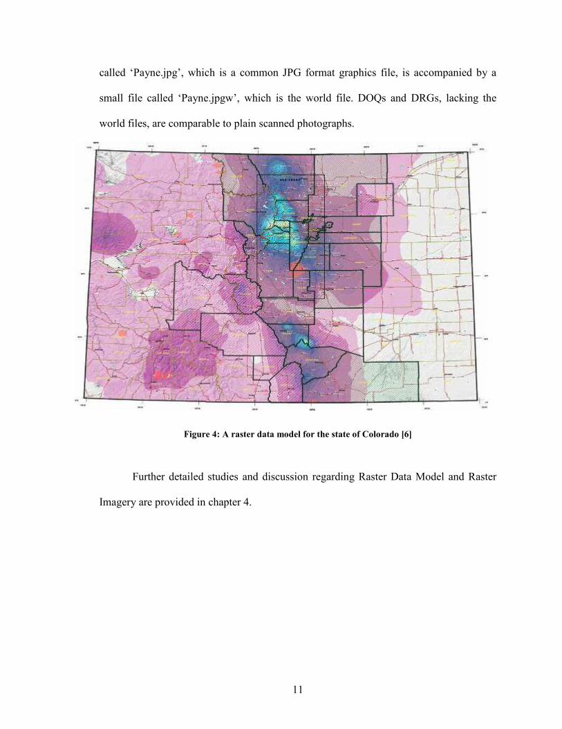
Figure 4: A raster data model for the state of Colorado [6]

Further detailed studies and discussion regarding Raster Data Model and Raster

Imagery are provided in chapter 4.

12

Chapter 3

Motivation and Objectives

GIS is a computer software which can be used to associate different geographical

features and information along with its description and attributes whereas a paper map

can be described as “What You See is What You Get” [9]. Map presented using the GIS

software can have multiple layers of information.

Maps can be useful in many different ways; for example, navigational purposes,

planning and development of a city, military purposes, and many more. Maps are not just

interactive, however as we work with them, we are capable of transforming the way the

data is displayed.

An area of interest (AoI) specifies the area within a map that is of interest to the

map user. As an example, the Department of Transportation (DoT) is concerned with

setting up a five year plan for the expansion of interstate highways within the

geographical boundaries of Payne County. The base map they have in consideration is the

map of ‘Oklahoma’ with multiple layers of information such as state boundaries, present

interstate highways within the state of Oklahoma, rivers, streams, and counties, etc. Since

the DoT’s area of interest for planning is surrounded by the geographic boundaries of

13

Payne County, the remaining segment of the map, except AoI, is not useful and moreover

it requires an enormous amount of storage space.

While exploring a map containing multiple layers of data, users begin with a

general view of the map and afterwards zoom into the area of concern. At present, GIS

desktop provides tools such as ArcView, ArcInfo, etc. that assist in retrieving vector data

by creating a wrapper around the area using a bounding box (Figure 5). A geographical

bounding box is a rectangle box which bounds a geographic feature or geographic data

set; moreover it is oriented to the X and Y axis with two coordinates each: X min, Y min

and X max, Y max.

Figure 5: Bounding box with zoom-in rectangle in ArcMap [4]

14

With the help of the zoom-in tool, users can zoom into their area of interest; the

rectangle drawn by the zoom-in tool represents the area to be zoomed-in. Questions such

as ‘What if the user is not interested in viewing the data of the entire area selected?’

arises. At present, there is no such technique available that could help users to select

multiple different segments of a map and extract those selected map segments from the

original map.

The user might want to perform analyses over multiple AoIs, which are separate

entities within the same map. However, with the aid of the existing system, users are able

to extract data (spatial/non spatial) covering the whole region more easily than getting

filtered out of areas that are not of interest. This makes the complex nature of the

interrelated data more difficult to use. In this situation, the user will have more data than

he wants, and the system will need to remove the excess data.

There exists no technology that allows naïve users to select raster data and

retrieve the vector data along with raster images associated with it. Users with advanced

knowledge of current software are able to extract vector and raster imagery through

multiple procedures. It is therefore essential to create a functionality that allows the users

to select raster data in a more user-friendly way and automatically retrieve the data

associated with the selected rater data.

15

Chapter 4

Background and Literature Review

The primary focus of this chapter is a review on the latest GIS technologies

together with the additional background study related with different GIS concepts and

applications. This review helps us to unfold the usability of common components under

desktop based GIS and provides us with the structure to proceed in this research.

4.1: GIS Software

In the modern world of automation, GIS is a significant tool which plays an

important function in shaping the world around us. An existing GIS software system is

comprised of an incorporated collection of software components, which includes end user

applications, geographic tools, and data access components. GIS is capable of integrating

and relating any data with a spatial component, regardless of the source of the data. For

example, you can combine the location of mobile workers located in real-time by using

GPS devices, in relation to the customer’s homes, located by address and derived from

the customer database [10]. The Environmental Science Research Institute (ESRI) is the

16

leading developer of geographic information systems software. We can categorize

ESRI’s GIS software packages into two major groups based on the functionality and

type; desktop GIS and server GIS. Within this research, we will focus primarily on

desktop GIS technology to implement the proposed approach for extracting raster and

vector for an AoI.

Figure 6: ESRI ArcGIS system achitecture [22]

4.1.1: Desktop GIS

A Desktop based GIS generally focuses on data utilization, however, it provides

tools to create, edit, import, map, query, analyze, and publish geographic information

[11]. As an example, ArcGIS desktop 9.2 helps in carrying out various GIS tasks like

viewing, data exploration, spatial analysis, Shapefile management, geoprocessing,

cartography, etc. on a desktop based environment. It is not only restricted to the tasks

mentioned, ESRI also allows users to do research and develop their personalized

17

extension to ArcGIS desktop by working with ArcObjects, the ArcGIS software

component library. Users are capable of mounting extension and custom tools with

standard windows programming interfaces, for instance, Microsoft’s VBA (Visual Basic

Application), Java, or C++. As a result, by using these programming interfaces, it is

possible to build object oriented executables or components that can be plugged within

the existing GIS applications. Within this research, we will be using Microsoft’s VBA for

the development and implementation of extended tools.

ArcInfo is among one of the ESRI’s GIS desktop products to build a

comprehensive desktop GIS. ArcInfo provides tools useful for data integration and

management, visualization, spatial modeling and analysis, and high-end cartography

along with single and multi-user environment. Furthermore, it can be used to gather,

build, and manage data, analyze geographic relationships, discover new information, and

produce publication-quality maps as ArcInfo provides additional facilities and tools [11].

ArcEditor give users advanced editing, data validation, and workflow

management tools to maintain the data integrity. Through ArcEditor, a user achieves the

capability to complete complicated spatial analysis. ArcEditor helps to handle complex

information, automate the editing workflow, and allows multiple users to update the same

data simultaneously [11].

With ArcView, users are capable of visualizing, exploring, and analyzing

geographic data, revealing underlying patterns, relationships, and trends. A user can use

ArcView to create maps, manage data, and perform spatial analysis [11].

18

Through ArcReader, users can view, print, explore, and query all maps and data

types. Furthermore, ArcGIS Desktop Extensions allows users to perform raster

geoprocessing, 3D visualization, and other geostatistical analysis [11].

Figure 7: ESRI ArcGIS framework [21]

4.1.2: Internet GIS

Internet GIS like ESRI’s ArcIMS (Internet Mapping Server) focuses on display

and query applications, as well as mapping of geographical data over the World Wide

Web. ArcIMS is an internet mapping server, designed for delivering dynamic maps and

GIS data over the Web, which is its primary focus. It provides a highly scalable

framework for GIS Web publishing that meet the requirements of corporate intranets and

the demands of worldwide internet accessibility. In general, ArcIMS users access GIS

19

web services via Web browsers using integrated HTML, Java, or .Net applications within

ArcIMS [3].

ArcSDE, a spatial database engine, is the GIS gateway to relational databases for

ArcIMS. ArcXML is ESRI’s flavor of XML and stands for Arc e-Xtensible Markup

Language [3].

4.2: Geographic Data Representation

The foundation of any map, created using desktop GIS, is the GIS database that

contains both data associated with the map (depicting location of geographical objects)

and its attribute (describing physical characteristics of each object). For example,

physical characteristics like timber species and/or non-physical characteristics like

estimated market value, representing attribute data contained by GIS, is used to examine

forestry problems [13].

Most importantly, GIS data components can be divided into spatial data and

attribute data. Geography of the earth’s surface, like its shape and position, can be

described by spatial data, while other attributes of geographic features in study, like its

characteristics or quality, can be described by attribute data. One can define attribute

elements as altitude, population, land use land cover, soil type, etc.

In general, spatial data (Figure 8) can be among one of these: a Point feature

(location), a line feature (road, river, or stream), a polygon feature (district, county,

region, etc.), or raster (aerial photography, digitized photo, images, etc.). Spatial data of

different or similar type is combined to form a data layer. A layer is considered the core

20

of a GIS based map and by stacking different layers on top of each other, users are able to

select different layers in order to create different visualization of a location.

Figure 8: Vector feature representations in a GIS [14]

4.3: Geodatabase

Geodatabase is the abbreviated form of ‘Geographic Database’. A geodatabase

represents geographic features and attributes like objects, where objects are stored within

a Relational Database Management System (RDBMS). A geodatabase is a container for

GIS data.

Geodatabase work across a range of RDBMS architecture comes in numerous

sizes, and the number of users (using it) can vary along time. They range from a small,

single user database built on the Microsoft Jet Engine (Microsoft Access) to a large work

group, division, and enterprise database accessed by multiple users. Two types of

21

Geodatabase implementations are available: Personal Geodatabase and Multi-user

Geodatabase.

Personal Geodatabase uses the file structure provided by Microsoft Jet Engine

database to preserve GIS data. They are similar to file-based workspaces and hold

databases up to 2 GB in size. Personal Geodatabase works perfectly with smaller data

sets for GIS projects within small work groups. Furthermore, Personal Geodatabase

supports single user editing. On the other hand, multi-user Geodatabase requires ArcSDE

as well as they are capable to work among a variety of RDBMS storage models (IBM

DB2, Informix, Oracle—both with and without Oracle Spatial, and SQL Server). Multi-

user Geodatabase are primarily used in work groups, divisions, and enterprise settings.

They acquire complete advantage of their underlying RDBMS to support:

• Tremendously large and continuous GIS databases

• Multiple real-time users

• Longer communication and versioned work flows

4.4: Geometry and Characteristics of Raster Data

In general, GIS represents geographic location by means of raster or vector

(feature geometry). In addition to vector features along with raster data sets, all other

spatial data types can be handled and stored within the relational tables allowing

opportunity to manage all geographic data within the RDBMS.

Vector features (geographic objects with vector geometry) are flexible and are

commonly used geographic data types, appropriate for representing features through

distinct boundaries, for instance, wells, roads, rivers, states, highways, railroad, parcels,

etc. We can define a feature as a simple object, with location stored as one of its

22

properties or fields within a row. Characteristically, features are spatially represented as

points, lines, polygons, or annotation and they are categorized as feature classes (Figure

8). Feature classes are compilation of features having identical category along with

common spatial representation and set of attributes (e.g., a line feature categorizing

streams).

Rasters are used to represent continuous geographic features or geographic

phenomenon (Figure 9) using layers, such as elevation, soil erosion, slope, aspect,

vegetation, temperature, annual rainfall, cloud dispersion, etc. Generally, rasters are

designed to store aerial photography as well as other images.

While representing rasters, image graphics and attributes are combined into a

unified data file. The area of study is subdivided within a fine network of grid cells

known as pixels. Every cell is associated with a number corresponding to a quantitative

or qualitative value that describes the site. For instance, the cell value may signify the soil

eroded from the agricultural land during different periods of annual rainfall or a number

that symbolizes a specified feature. Particular to images, (digital photograph) reflectance

among different wavelengths are stored in separate layers and by using ‘Overlay’

procedure, an image can be reconstructed. Raster data compilation requires intense

amounts of data storage area as they tend to accumulate information with reference to

each and every point, and although they imitate computer data architecture, evaluation

within rasters is fast. Furthermore, raster images are enhanced in representing spatial data

and, thus, raster systems have considerably extra analytical control. Raster systems work

outstandingly while executing analysis associated with natural resources and agricultural

23

data, because most of the data used for these areas are available in the form of satellite

images [4].

Figure 9: Raster data sets representations [15]

A GIS database is considered as a collection of maps. The main advantage of a

raster system is that the images are separated as individual layers and are capable of

joining simultaneously, if so desired, via overlaying. This structure provides an advantage

to researchers who like to view an image within a particular wavelength, for example,

near infrared. Complex images can be created with a combination of arrangement of

vector and raster layers. An advantage of GIS maps is they are not subjected to a

particular scale that means that the data layers that are compiled from paper maps of

different scales, covering the same region can be combined together. All spatial data in

24

GIS needs to be georeferenced according to the location of an image or layer in space as

defined by a particular coordinate system [4].

The vector data layers have features such as points, lines, and polygons whereas

the raster layers do not include features by itself and the closest equivalent would be a

pixel. The most important difference between the raster and the vector is that, in vector

space, objects are typically well defined with their attributes and spatial relations

determined, while, in raster space, normally this is not the case. The distinction plays an

important role as (in vector space) the object extends and spatial relations are well-

defined and the operations and techniques for manipulating and querying their properties

is different from unprocessed objects on a raster image [4].

4.5: Georeferencing Vector and Raster

Extracting information from raster data over a set of boundaries within a raster

and vector data set is complex. The assumption of this problem is that the raster and

vector data sets overlap geographically and both data sets are described by sufficient

georeferencing information for data fusion [16].

Data sets georeferencing, or geographic referencing, is the name specific to the

procedure of assigning values of latitude and longitude to features on a map. Latitude

(lat) and longitude (long) represent points in a three-dimensional (3D) space, whereas

maps are represented naturally in two-dimension (2D). With the introduction of computer

technology, we are able to store maps as digital images as they characterize raster

information like 2D image information. The procedure involved in georeferencing a

digital map image can be defined as the difference between map image specification

25

types; but at the end, we are capable to recover the lat/long coordinates for any given

point on the georeferenced map. Latitude and longitude identify a point on a 3D model of

the Earth; at the same time, map coordinates symbolize a pixel – a row and column

location on a 2D grid obtained after projecting a 3D model of the Earth onto a plane.

Georeferencing is helpful as the lat/long coordinates defines the location of an object on

the Earth’s surface. It is simple to represent 2D maps along with distance measurement,

while 3D coordinates are precise but cumbersome and do not possess standard length for

different degrees of latitude and longitude [16].

ArcGIS software, with its components that incorporate ArcView and

ArcExplorer, provided by ESRI, is one of the GIS systems that are capable of

acknowledging geospecific data and providing geographic referencing. There is a

tremendous amount of information available associated with georeferencing; however,

the knowledge required to properly georeference a single image can be overwhelming.

The complications appear as we try to project a 3D surface like the Earth, onto a 2D

object like a map. Understanding something about this process goes a long way towards

understanding why certain parameters are needed to geographically orient a digital image

[16].

4.6: Projections

Projection of a map is a plane surface representation of the two-dimensional

curved surface of the earth. “The term "projection" here refers to any function defined on

the earth's surface and with values on the plane, and not necessarily a geometric

projection” [25]. For example, Azimuthal equal-area, Universal Transverse Mercator

26

(UTM), Lambert Conformal Conic, Lambert Equal Area, etc. are some of the common

GIS projections.

4.7: Georeferencing Coordinate Transformations

The Georeferencing system is built around coordinate transformations to and from

three types of location representations: 2D map pixels (column and row), 3D lat/long

coordinates, and 2D Universal Transverse Mercator (UTM) values (Figure 10). These

transformations are shown in Figure 10. The motivation for the transformations between

a 2D map and 3D lat/long coordinate systems is obvious, because one would like to know

the lat/long values of any pixel in a georeferenced image. The third location

representation, the UTM coordinate system, is a Cartesian coordinate system useful for

specifying a number of points on a map without having to refer to latitude and longitude

[16].

Figure 10: Types of coordinate transformations [16]

27

Furthermore, UTM values facilitate metric distance calculations, which are

difficult in lat/long coordinates where the distance between two adjacent degrees is

dependent upon their location relative to the equator and the prime meridian.

4.8: Literature Review

Amar Gupta [4] proposed a prototype tool during his research work for his

Masters Thesis “Grid Based Raster Selection and Vector Extraction” in December 2006.

This tool is capable of extracting vector data using a customized ArcGIS desktop

application. However, this prototype tool was unable to extract raster and vector data

simultaneously. Moreover, it has no control over reducing data storage space. Also, if

users want to extract multiple feature layers, we would have to run the application over

and over again without having initial selections made over the raster imagery.

Within this research effort, we develop a tool that is capable of extracting raster

and vector data simultaneously and reduce the data storage size. Moreover, it makes it

possible to extract multiple vector data layer without resetting the Area of Interest

selected by the user.

28

Chapter 5

Methodology and Proposed Solution

This chapter outlines the methodology for the problem stated in chapter 3. In

addition, this chapter also describes the proposed framework.

5.1: Methodology

The methodology is further divided into the following steps:

5.1.1: System setup and software requirement

The system setup requires installation of ArcGIS Desktop and ArcMap on the

Windows environment. The following is the detailed list of software required for the

implementation.

• Operating system – Microsoft Windows 2000 server or Windows XP

• Desktop mapping software – ArcGIS desktop 9.2, ArcMap

• Object library for Macro- ArcObjects

• Programming language – Microsoft VBA

• CPU Speed –1.0 GHz or higher

• Memory/RAM-512 MB minimum, 1 GB recommended or higher

29

• Display properties-Greater than 256 color depth

5.1.2: Collection and Conversion of Spatial Data into a Geodatabase

After setting up the system with the essential software requirements mentioned

above, the collection of different types of GIS datasets is required. The different GIS

datasets include vector and raster data. All the required data is provided by the

Department of Geography, Oklahoma State University. The maps of various Oklahoma

state counties are used as the test dataset. The data used in this research is pre-projected

in UTM 13N, 14N, and 15N projections.

5.2: Proposed Solution

The solution to the problem explained in chapter 3 is described in this chapter. A

GIS tool is developed in order to solve issues related to simultaneous selection,

extraction, and speedy analyses and decrease the file storage size. This GIS tool requires

ESRI tools like ArcMap, ArcCatalog, ArcToolbox and ArcObjects. The programming

language we will use to create user interface is Microsoft’s Visual Basic for Applications

(VBA).

The initial step is to introduce the imaginary raster grid on top of the map layers.

Next, the raster cells are selected from the imagery after which the raster and vector data

that belong to the geography of the chosen cells or AoI are extracted. A cell can be

described as the minimal rectangular unit (pixel) for the raster grid. Cells are used to

define the resolution of an image. As the cell size increases, the resolution of an image

decreases and vice versa. In this research, a user is able to define the cell size by entering

30

an integer value. Existing GIS technology offers different ways to select vector data on

maps; however, extracting raster data types is still an area of research. In this research,

we apply an approach based on grids, which will assist further in selecting the Area of

Interest within the raster images. To improvise the map browsing process as well as to

make it easier for the user to deal with complicated maps, a transparent grid is provided

above the other map layers. With this grid based approach, it becomes more of an

advantage as it is easier for the user to browse through a map, thus reducing the

complexity of a map with increasing user-interaction. Clearly, if this method is applied to

mobile devices like cell phones, we would have to deal with a number of restrictions such

as small display size, inadequate processing power, low bandwidth, etc. On the other

hand, it can be used as an alternate for slide bar and map menus, providing the user with a

swift and spontaneous interface for zooming and pan methods. Grid interaction can be

understood as a virtual equivalent to the physical tasks such as moving or folding maps

[4].

In order to work together with a grid, an arbitrary pointing tool is required for

movement and selection within the map. Users can simply go all the way across the map

in order to select the Area of Interest and highlight the selected cells. With the help of

World file, typically an ASCII file along with raster images, the projected solution

generates a provisional polygon ‘Shapefile’ (*.shp) including the characteristics of

selected raster cells. This Shapefile is termed as a ‘Clipper’, which is sequentially used

for clipping the objective vector data. A ‘clip’ method will be executed which applies a

clipper as a cookie cutter over the target area (AoI). In order to get the desired results, we

will not change any characteristics of the AoI. After getting the output vector data, raster

31

data falling under the AoI can be clipped and can be merged along with the vector data

layer produced from the previous steps. Users will be able to perform any desired

analytical work on the data extracted using the above procedures on the AoI. This

procedure reduces the amount of file storage space that was initially required, thus,

solving data storage problems. So far, no one has introduced a tool that can select and

extract raster and vector data simultaneously from a map by selecting the AoI.

The subsequent parts will describe the proposed solution given above, in detail,

as flowchart and block diagrams.

32

Figure 11: Block diagram for steps and procedures required

Add the Input Layers Within

Map

Introduce an Imaginary Raster Grid Over

The Map

Select Grid Cells Defining The Area of Interest

World Coordinate Conversion Procedure Applied To

Image Coordinates

Create Temporary Shapefile Used as a Clipper For Clipping Procedure

Clip the Raster Data Using Shapefile Created

In Previous Step

Using Same Shapefile of Previous Step

Clip Vector Data (Feature Layer)

Overlay All Clipped Data Layers

Together For Visualization

Final Is the Desired Output With a Reduced Amount

Of Data Storage Space Required

33

Figure 12 : Flow chart illustrating step by step procedures for implementation

Are Layers Active?

Prompt User to Select Layers

Ask User to Specify Cell Size in Meter as Units

Select AoI Using Mouse

Pointer

Convert Coordinates of AoI to World

Coordinates

Add and Select Input Data

Layers from Disk

Is User Done Selecting

Cells?

Create a Clipper

Yes

Yes

No

No

cont

34

Figure 13: Flow chart illustrating step by step procedures for implementation (cont.)

Does Clipper Have the Same Projection as Target Data?

Display Error Message

Clip Target Raster Data

Add Clipped Layer to Table of Content As Map Layer

Merge all Temporary Saved Layers

The Extraction is Complete

Save Output at a Different Storage Location

Yes No

Ask User to Specify Vector Layer to be

Extracted

Ask User If More Vector Layers to Be

Clipped

Yes No

35

Chapter 6

Implementation and Conclusion

In this chapter, we will discuss the implementation procedures of the proposed

solution and test the resulting tool using various different types of data.

As mentioned earlier, GIS maps containing raster and vector data require a large

storage space and the major part of the problem lies in the extraction of information from

both these data types simultaneously. This gives us a motivation to design and develop a

tool that could facilitate users to select and extract several different areas of interest

within the same map. Extraction of raster and vector data types provides a more

convenient mechanism to perform analytical work such as spatial analysis that includes

environmental and socioeconomic data. Furthermore, this specialized application solves

issues related to storage space since raster data types have large file sizes (varying from

few mega bytes to hundreds of mega bytes).

6.1: Implementation

ESRI’s ‘ArcObjects’ library provides us with a development platform, which we

use within this research work in conjunction with the ‘ArcGIS’ family of applications

36

such as ‘ArcMap’ and ‘ArcToolbox’. The ArcObjects library components represent a

variety of functionality that exists within ‘ArcInfo’ and ‘ArcView’ for software

developers. Visual Basic for Applications (VBA) is the most familiar programming

interface used by developers to modify the ArcGIS Desktop applications; VBA comes

embedded inside ArcCatalog and ArcMap. Furthermore, using VBA, we can manipulate

the application framework that already exists in ArcMap for all-purpose data

management and map presentation tasks. The ESRI ArcObjects library is always

accessible in the VBA environment [17]. Developers, along with adequate expertise, can

create self-tailored applications in order to avoid the initial application structure of

ArcMap and ArcCatalog.

The encoded interface is used to create stand-alone executables or components,

which can be, later, embedded within existing GIS applications. There are a number of

benefits in using this technique for solving analytical and storage space issues that we

will discuss further in chapter 7. There are ways to customize an ArcGIS desktop

application in order to improve productivity. For this research, we will be using ArcMap

to develop a customized application.

The feature data (vector imagery data) used for testing and implementation

purpose has been provided by the Oklahoma Center for Geospatial Information (OCGI)

[20]. The format of data provided by OCGI is either geographic data or projected data.

We will use geographic data and then re-project that data in UTM 13N, UTM 14N, and

UTM 15N projections. Raster data (Image data) imagery has been provided by OCGI;

these are 2003 National Agriculture Imagery Program (NAIP) countywide mosaic images

which are projected in UTM Zonal projections (Aerial Photo Images). The raster data is

37

‘MrSID’ images that come along with the “world” file, “.aux” file, and a “.txt” files for

each county mosaic.

6.1.1: Testing and Results

We, now, proceed with the screenshots of the customized application, developed

using ArcObjects and VBA. After creating a custom toolbar and writing all the codes, we

proceed with testing the functionality of the tool using different data layers which we had

already stored on the hard drive. To test the tool prototype, start by adding the data layers

within ArcMap as shown in Figure 14.

Figure 14: Adding data layers to the ArcMap application

38

After adding all the raster and vector layers within ArcMap document, we can see

the layers added on the left hand side of the window in the ‘Table of Content (TOC)’

under ‘Layers’ (See Figure 15).

Figure 15: Showing layers added and shown in Table of Content

39

After adding and selecting data layers, we will, now, move to the next step. Begin

by clicking the ‘Launch’ button on the ‘Extraction toolbar’ as shown in Figure 16. The

extraction tool is now launched.

Figure 16: Showing customized application launch dialogue

40

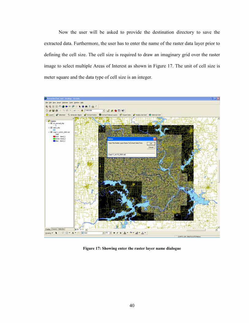
Now the user will be asked to provide the destination directory to save the

extracted data. Furthermore, the user has to enter the name of the raster data layer prior to

defining the cell size. The cell size is required to draw an imaginary grid over the raster

image to select multiple Areas of Interest as shown in Figure 17. The unit of cell size is

meter square and the data type of cell size is an integer.

Figure 17: Showing enter the raster layer name dialogue

41

By clicking the ‘Display AoI Grid’ button, you can see the raster grid created over

the raster imagery (See Figure 18). The user can hide the display grid by clicking the

‘Hide AoI Grid’ button. The grid created has spatial reference inherited from the raster

imagery added as a base image (Raster Image).

Figure 18: Showing raster grid displayed over a raster layer

42

Next, select the Area of Interest (AoI) by using the mouse cursor as shown in

Figure 19. Each selected cell has a cell size specified by the user in previous steps.

Figure 19: Showing user selected Area of Interest

43

After the user is done with selecting the cells for the Area of Interest, in order to

extract raster and vector data, they would need to generate a ‘clipper’ (polygon shape

file). Click the ‘Generate Clipper’ button in order to create the clipper shapefile, which is

stored at a temporary location, and this is shown in Figure 20. The Clipper layers are then

added within the TOC.

Figure 20: Showing clipper layers created and added in Table of Content

44

After executing the previous step, a clipper layer is added to the Table of Content

(TOC). Now we start extracting data layers, beginning with extracting raster data layer.

To start raster extraction click the ‘Extract Raster’ button (Figure 21). The extraction

procedure is a time consuming process depending upon AoI selected and raster layer size

and the progress is shown at the bottom task pane (as shown in Figure 21).

Figure 21: Showing raster extraction procedure and its progress

45

After the raster extraction is completed, the resulted raster layers will be visible

on top of all the map layers. Click the ‘Extract Feature Layers’ button to start extracting

the feature layers (vector data layers) as shown in Figure 22. The user will be prompted

to enter the layer name in order to ‘clip’ the layer. A user can clip multiple feature layers

one after another (Figure 22).

Figure 22: Showing clipping feature layer dialogue

46

Before proceeding further, the application will confirm whether more layers need

to be clipped as shown in Figure 23 and once the user is done clipping, type “No” to stop

extracting the feature layers. All clipped layers will be added to the Table of Content

(Figure 23).

Figure 23: Showing extract more layer dialogue

47

Figure 24 shows the ArcMap window with all clipped layers including the

original data layers where the user has the choice to remove the original layers from the

map.

Figure 24: Showing extraction complete dialogue

48

Finally, to ‘export’ the clipped Feature Layers (Vector data layers only), click the

‘Export Data’ button, and enter the path to the directory to export and save the output

layers as shown in Figure 25.

Figure 25: Showing export data and enter the path to save output layers

49

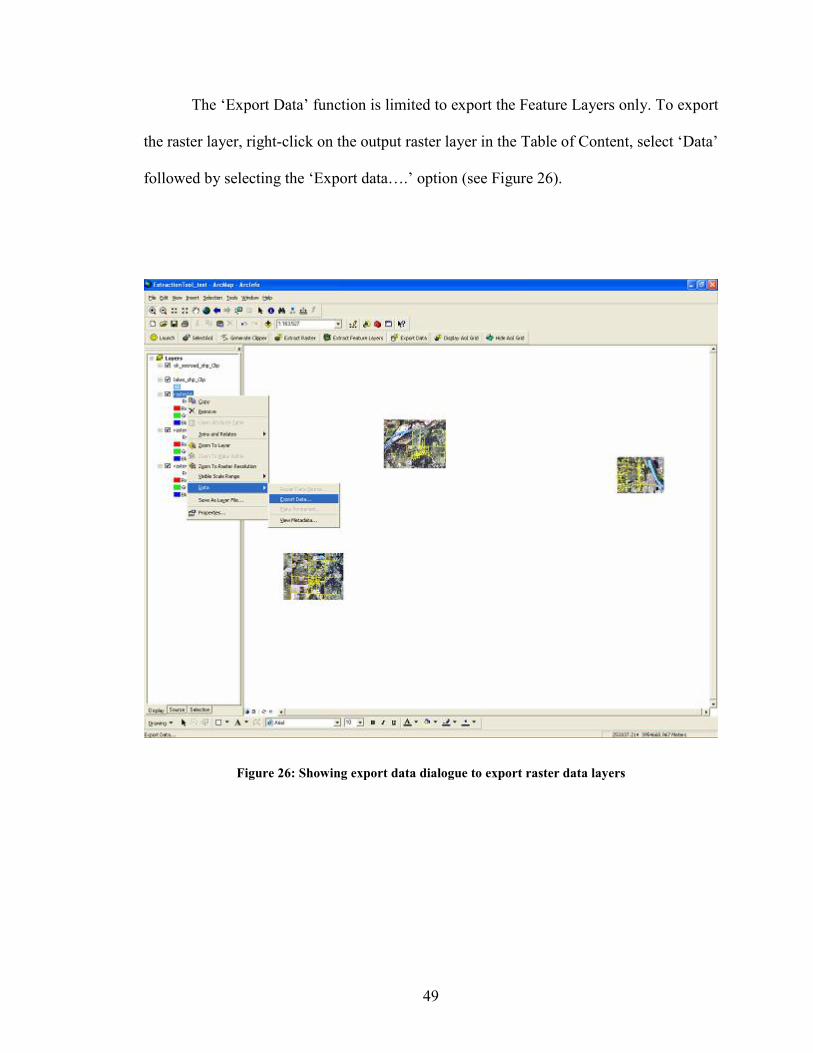
The ‘Export Data’ function is limited to export the Feature Layers only. To export

the raster layer, right-click on the output raster layer in the Table of Content, select ‘Data’

followed by selecting the ‘Export data….’ option (see Figure 26).

Figure 26: Showing export data dialogue to export raster data layers

50

The output raster data layer has the exact same spatial reference, inherited from

the original raster data layer. To view raster layer properties, double click on the raster

layer from the Table of Content as shown in Figure 27.

Figure 27: Showing raster layer Properties dialogue

6.2: Conclusion

In this work, we develop a prototype tool that can be used within a desktop GIS

environment. This tool gives us the capability to select a user-defined Area of Interest

(AoI), along with the functionality to extract multiple Feature layers (Vector data layers)

51

and Raster data layer. Moreover, it automatically extracts Feature data layer to a user-

specified location. The most useful functionality of this tool is its capability to reduce the

size of Raster data. The size of raster data layer reduced is directly relative to the AoI

selected by the user. No compression technique is used to reduce the Raster data file size.

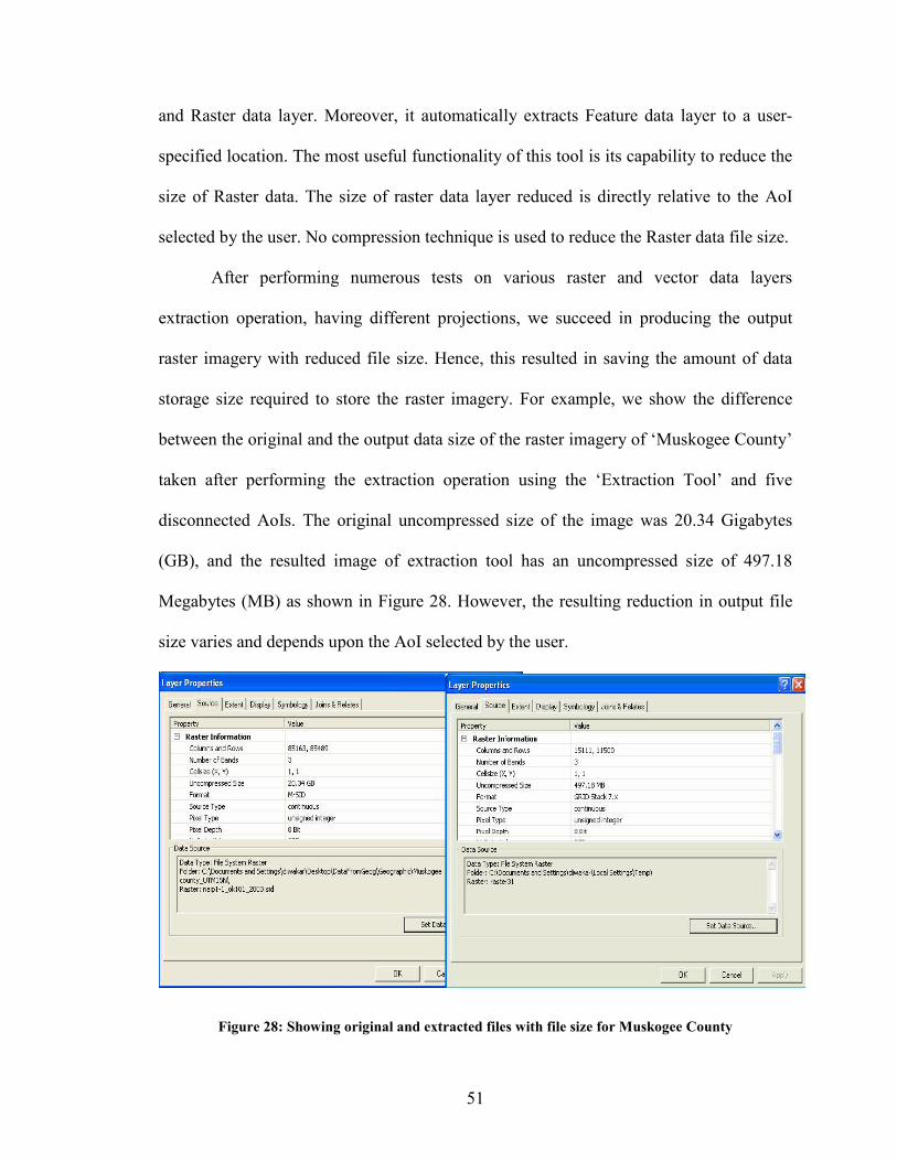
After performing numerous tests on various raster and vector data layers

extraction operation, having different projections, we succeed in producing the output

raster imagery with reduced file size. Hence, this resulted in saving the amount of data

storage size required to store the raster imagery. For example, we show the difference

between the original and the output data size of the raster imagery of ‘Muskogee County’

taken after performing the extraction operation using the ‘Extraction Tool’ and five

disconnected AoIs. The original uncompressed size of the image was 20.34 Gigabytes

(GB), and the resulted image of extraction tool has an uncompressed size of 497.18

Megabytes (MB) as shown in Figure 28. However, the resulting reduction in output file

size varies and depends upon the AoI selected by the user.

Figure 28: Showing original and extracted files with file size for Muskogee County

52

Our tool also allows us to select multiple disconnected AoIs. Hence, it gives the

user a capability to select 2, 3, 4 or more AoIs from the same original image and analyze

each of these AoIs. All the selected AoIs can be displayed at the same time.

53

Chapter 7

Challenges and Future Work

In this chapter, the assumptions made and the challenges faced during the

implementation of the proposed solution are stated. Furthermore, it includes a brief

overview of limitations of the developed application tool along with the future work that

can be done considering this tool as a prototype.

The assumptions made in this work are stated below.

• The Feature Data Layers (Vector data) are projected in the same projections

as the Raster Data (Raster Image).

• The Raster Data Layer has pre-specified geo-coordinates, i.e. it contains a

world file.

• Only Raster Data Layer has to be exported and saved by the user using

‘Export data’ tool from ‘tools’ menu.

• All the original data layers must be removed from ‘Table of Contents’

before performing Export Data Procedure on clipped Feature layers.

One of the challenging tasks was to obtain imagery with the same projection. The

data, provided by different agencies, are in various projections or with no pre-defined

54

projections. The feature data (Vector Data) used for this research is geographic data

obtained from OCGI. In order to get the same projection as Raster Data, we projected

Feature Data using ‘ArcToolbox’ Tool, i.e. “Data Management Tools > Projections and

Transformations > Feature > Project” tool. This tool is limited to extract data only from

projected geo-referenced data, i.e. raster and vector. Data, having no or missing spatial

reference (Projections), may result in unwanted results.

In the future, this tool can be customized for its use over the Internet and to

providing internet users with an ability to select an Area of Interest and extract raster and

vector data concurrently.

55

BIBLOGRAPHY

[1] What is GIS, the guide to Geographic Information Systems, GIS information on web, http://www.gis.com/whatisgis/index.cfm, Date of last access: February 07, 2007.

[2] Three views of a GIS, http://www.esri.com/software/arcgis/concepts/three-

views.html, Date of last access: February 07, 2007. [3] Chudiwale, Varun, “Development of processes for online GIS data selection,

extraction, and aggregation using ArcIMS and .NET technology”, Master thesis, Computer Science, Oklahoma State University, December 2005 .

[4] Gupta, Amar, “Grid based raster selection and vector extraction”, Master Thesis,

Computer Science, Oklahoma State University, December 2006. [5] Geographic Information System, guidelines on the application of GPS in modern

mapping and GIS technologies to population data, http://www.unescap.org/stat/pop-it/pop-guide/gis_ch04.pdf , Date of last access: February 13, 2007.

[6] Raster Data Model, http://www.gis.com/implementing_gis/data/raster.html, Date of

last access: February 14, 2007. [7] Carswell, James D., “Using raster sketches for digital image retrieval”, PhD thesis in

Spatial Information Science and Engineering, The University of Maine, May 2000. [8] The GIS Primer, Fundamental concepts,

http://www.innovativegis.com/basis/primer/concepts.html, Date of last access: February 14, 2007.

[9] GIS in Our World, http://www.esri.com/company/about/facts.html, Date of last

access: February 15, 2007. [10] Why Use GIS? http://www.gis.com/whatisgis/whyusegis.html, Date of last access:

February 18, 2007. [11] ArcGIS Desktop Products, http://www.esri.com/software/arcgis/about/desktop.html,

Date of last access: FEB 18 2007. [12] ArcGIS-The complete geographical information system,

http://www.esri.com/software/arcgis/graphics/arcgis92_sm.jpg, Date of last access: February 21, 2007.

[13] Introduction to data analysis using geographic information system,

http://www.extension.umn.edu/distribution/naturalresources/DD5740.html, Date of last access: February 21, 2007.

56

[14] Feature class basics, http://webhelp.esri.com/arcgisdesktop/9.2/published_images/Feat%20Class%20PointLinePoly.gif, Date of last access: February 21, 2007.

[15] GIS spatial data model, Rasters,

http://gis.washington.edu/cfr250/lessons/introduction_gis/images/grid_data_model_0.gif, Date of last access: February 22, 2007.

[16] Bajcsy, Peter, Peter Groves, Sunayana Saha, and Tyler Alumbaugh, “Decision

Support using data mining methods and geographic information”, Technical Report NCSAALG-03-0002, February 2003.

[17] ArcObjects online, Copyright © Environmental Systems Research Institute, Inc.

http://edndoc.esri.com/arcobjects/8.3/, Date of last access: February 23, 2007.

[18] Mitchell, Andy, ‘‘The ESRI guide to GIS analysis, Volume 1: Geographic Patternsand Relationships’’. ISBN: 1879102064 ESRI Press, Redlands, CA, 1999.

[19] Customize ArcGIS to meet your unique needs,http://www.esri.com/software/arcgis/about/desktop_gis.html, Date of last access:July 19, 2007.

[20] Oklahoma Center for Geospatial Information (OCGI), Department of Geography atOklahoma State University, http://www.ocgi.okstate.edu/ Date of last access: July15, 2007.

[21] ArcGIS Framework, http://www.esriuk.com/products/product.asp?groupid=15&mode=groupoverview, Date of last access: July 23, 2007.

[22] Developers Resources,

http://www.esri.com/software/arcgis/arcgisengine/about/dev-resources.html, Date of last access: FEB 23 2007.

[23] GIS Basics, http://www.gis.unbc.ca/courses/geog300/lectures/lect2/rasterv.gif, Date

of last access: July 30, 2007.

[24] Electric Facilities, http://www.esri.com/mapmuseum/mapbook_gallery/volume19/electric3.html, Date of last access: July 30, 2007.

[25] Map Projections, http://en.wikipedia.org/wiki/Map_projection, Date of last access:

August 15, 2007.

57

APPENDIX A

APPLICATION FUNCTION AND SUBROUTINE

To build a customized application, start a new ArcMap document and open a new

empty map as shown in Figure 29.

Figure 29: Showing an empty ArcMap application

58

Select ‘Customize’ on the Tools menu or right-click any open toolbar and select

customize from the menu. Click the command tab and create your own toolbar. Now add

new user interface control (UIControl) as shown below in Figure 30.

Figure 30: Showing customizing application using customize toolbox

59

Once the customized toolbar is created along with UIControl buttons added, click

and drag the UIButtonControl from the command list to the new toolbar. Right-click on

any button within custom toolbar and then select view source (see Figure 31). Now, begin

by writing the code to define the functionality of each UIControl buttons.

Figure 31: Showing procedure to open visual basic editor (VBE)

60

After the visual basic editor is opened, type the name of the application and save

the file. Within ‘ThisDocument’ (code) window (as shown in Figure 32), start writing

your customized code (refer Appendix A for code listings) using the ArcObjects library

and Visual Basic language. After writing the code for the custom toolbar, debug and test

it for errors and proper functionality, then, save the project and close the visual basic

editor.

Figure 32: Showing visual basic editor and code window

61

For later use, the user can ‘select’ and ‘remove’ the customized toolbar for

visualization as shown in Figure 33.

Figure 33: Selecting the customized toolbar for visualization

62

The following is the customized ArcMap application source code written in VBA using ArcObjects.

This Document:

‘This subroutine clears the graphic container elements Public Sub ClearGraphicContainer() Dim pMxDoc As IMxDocument Dim pGraphicsContainer As IGraphicsContainer Set pMxDoc = Application.Document Set pGraphicsContainer = pMxDoc.FocusMap pGraphicsContainer.DeleteAllElements pMxDoc.UpdateContents pMxDoc.ActiveView.Refresh End Sub

‘This subroutine zooms in to a particular layers extent Public Sub ZoomToLayer() Dim pMxDoc As IMxDocument Dim pMap As IMap Dim pActiveView As IActiveView Dim pContentsView As IContentsView Dim pLayer As ILayer Set pMxDoc = Application.Document Set pMap = pMxDoc.FocusMap Set pActiveView = pMap Set pContentsView = pMxDoc.CurrentContentsView 'If Not TypeOf pContentsView.SelectedItem Is ILayer Then Exit Sub Set pLayer = SearchLyr("Clipper") 'Set pLayer = pContentsView.SelectedItem pActiveView.Extent = pLayer.AreaOfInterest pActiveView.Refresh End Sub

‘This subroutine clips the target raster Public Sub clipRaster() Dim pRasterLayer As IRasterLayer Dim pMxd As IMxDocument Set pMxd = ThisDocument

63

Dim pMap As IMap Set pMap = pMxd.FocusMap Dim pRaster As IRaster

Set pRasterLayer = pMap.Layer(SearchRaster) Set pRaster = pRasterLayer.Raster

Dim pTransOp As ITransformationOp Set pTransOp = New RasterTransformationOp Dim pClipEnv As IEnvelope

'getting the clipping feature

Dim pActiveView As IActiveView Set pActiveView = pMxd.ActiveView Set pClipEnv = pActiveView.Extent.Envelope Dim pGeoDS As IRasterDataset Set pGeoDS = pTransOp.Clip(pRaster, pClipEnv) Dim pR As IRaster Set pR = pGeoDS.CreateDefaultRaster Set pRasterLayer = New RasterLayer pRasterLayer.CreateFromRaster pR pMap.AddLayer pRasterLayer pActiveView.Refresh End Sub

‘This function search feature layer and return the layer if found Public Function SearchLyr(LyrName As String) As ILayer Dim pMxDoc As IMxDocument Set pMxDoc = ThisDocument

Dim pMap As IMap Set pMap = pMxDoc.FocusMap

Dim pEnumLayer As IEnumLayer Set pEnumLayer = pMap.Layers

Dim pLayer As ILayer Dim pLayerReq As ILayer

Set pLayer = pEnumLayer.Next Do

64

If pLayer Is Nothing Then Exit Do If pLayer.Name = LyrName Then Set pLayerReq = pLayer End If Set pLayer = pEnumLayer.Next Loop

Set SearchLyr = pLayerReq End Function ‘This function search raster layer Public Function SearchRaster() As Long Dim pMxDoc As IMxDocument Set pMxDoc = ThisDocument

Dim pMap As IMap Set pMap = pMxDoc.FocusMap Dim idx As Long idx = 0 Dim pEnumLayer As IEnumLayer Set pEnumLayer = pMap.Layers

Dim pLayer As ILayer Dim pLayerReq As ILayer

Set pLayer = pEnumLayer.Next Do If pLayer Is Nothing Then Exit Do If TypeOf pLayer Is IRasterLayer Then Exit Do End If idx = idx + 1 Set pLayer = pEnumLayer.Next Loop SearchRaster = idx End Function Public Function Celing(Number As Variant) As Variant If Number = Int(Number) Then Celing = Number Else Celing = Int(Number) + 1 End If End Function

65

‘This subroutine call form in order to enter grid cell size in meters Public Sub Cell_Size()

frmSize.txtcelsz.Text = "" 'loop till cell size is not selected frmSize.Show cellsize = frmSize.txtcelsz.Text

Dim pMxDoc As IMxDocument Set pMxDoc = ThisDocument Dim pMap As IMap Set pMap = pMxDoc.FocusMap

'Creating a raster layer Dim pRasterLy As IRasterLayer Set pRasterLy = New RasterLayer Set pRasterLy = pMap.Layer(SearchRaster())

'Setting raster property Dim pRasProp As IRasterProps Set pRasProp = pRasterLy.Raster Dim height, width As Double height = pRasProp.height width = pRasProp.width

lRows = Celing(height / cellsize) lCols = Celing(width / cellsize) totalcells = lRows * lCols ReDim rowcollist(100000) cellcnt = 0 End Sub “This subroutine is called when select AoI button is clicked Public Sub btnSelectAoI_Select()

datToday = Now If cellsize <= 0 Then MsgBox "Please select cell size", vbExclamation, datToday Exit Sub End If End Sub 'Generate clipper and clip

66

Private Sub btnClip_Click() datToday = Now Dim check check = True Do While check = True If (cellsize <= 0) Then MsgBox "select cell size", vbExclamation Exit Sub End If Dim pMxDoc As IMxDocument Set pMxDoc = ThisDocument 'remove old clip result layer Dim pLayerDel As ILayer 'delete old clip result file Dim tmp As Object Set tmp = CreateObject("Scripting.FileSystemObject") If tmp.FileExists("C:\TEMP\shape\ClipResult_Clipper.shp") Then tmp.DeleteFile ("C:\TEMP\shape\ClipResult_Clipper.*") End If 'Getting the fearure name to clip Dim Message, Title, Default ', 'FeatureName As String Message = "Type The Feature Layer Name To Extract Data From" ' Set prompt. Title = "Feature Name" ' Set title. Default = "" ' Set default. 'Display message, title, and default value. FeatureName = InputBox(Message, Title, Default) 'Including input layer and its feature class. Dim pLayer As ILayer Set pLayer = SearchLyr(FeatureName) Dim pInFeatLyr As IFeatureLayer Set pInFeatLyr = pLayer Dim pInTable As ITable Set pInTable = pLayer ' First: Include input feature class.

' Second: Include Itable interface from Layer not from FeatureClass ' Third: Input feature class properties i.e shape type etc. needed for the output. Dim pInFeatClass As IFeatureClass

Set pInFeatClass = pInFeatLyr.FeatureClass

67

'First: Get the layer used for clipping ' Second: Include Itable interface from Layer not from FeatureClass Set pLayer = SearchLyr("Clipper")

Dim pClipTable As ITable Set pClipTable = pLayer ' check for errors

If pInTable Is Nothing Then

MsgBox "Table QI failed" Exit Sub End If

If pClipTable Is Nothing Then MsgBox "Table QI failed" Exit Sub End If ' Defining the o/p feature class name and shape type inherited

' from input feature class properties Dim pFeatClassName As IFeatureClassName

Set pFeatClassName = New FeatureClassName With pFeatClassName .FeatureType = esriFTSimple .ShapeFieldName = "Shape" .ShapeType = pInFeatClass.ShapeType End With ' Set o/p destination and feature class name

Dim pNewWSName As IWorkspaceName

Set pNewWSName = New WorkspaceName pNewWSName.WorkspaceFactoryProgID = "esriCore.ShapeFileWorkspaceFactory.1" pNewWSName.PathName = "C:\TEMP\shape\" Dim pDatasetName As IDatasetName

Set pDatasetName = pFeatClassName pDatasetName.Name = FeatureName + "_Clip" Set pDatasetName.WorkspaceName = pNewWSName

' Setting tolerance: Passing 0.0 causes the default tolerance to be used.

' The default tolerance is 1/10,000 of the extent of the data frame's spatial domain

68

Dim tol As Double tol = 0# ' Perform the clip

Dim pBGP As IBasicGeoprocessor Set pBGP = New BasicGeoprocessor Dim pOutFeatClass As IFeatureClass Set pOutFeatClass = pBGP.Clip(pInTable, False, pClipTable, False, _ tol, pFeatClassName) ' Add the output layer (clipped features) to the map

Dim pOutFeatLyr As IFeatureLayer Set pOutFeatLyr = New FeatureLayer Set pOutFeatLyr.FeatureClass = pOutFeatClass pOutFeatLyr.Name = pOutFeatClass.AliasName pMxDoc.FocusMap.AddLayer pOutFeatLyr 'ask user if wants to extract more layers...

Dim Message1, Title1, Default1, MyValue As String

Message = "Would You Like To Extract More Frature Layers ? (case sensitive: Yes/No)" ' Set prompt. Title = "Extract More Layers ?" ' Setting title. Default = "No" ' Set default. 'Display message, title, and default value. MyValue = InputBox(Message, Title, Default)

If MyValue = "No" Then 'removeing the temp clpper layer

Set pLayerDel = SearchLyr("Clipper") ' Pass the requied layer name. If Not pLayerDel Is Nothing Then pMxDoc.FocusMap.DeleteLayer pLayerDel End If

'delete clipper file Set tmp = CreateObject("Scripting.FileSystemObject") tmp.DeleteFile ("C:\TEMP\shape\Clipper.*") check = False cellcnt = 0 Exit Do Else: check = True End If cellcnt = 0

69

Loop MsgBox "Data Has Been Extracted Successfully", vbInformation, datToday MsgBox "Extracted Layers Can be Saved Now", vbInformation, datToday End Sub ‘This subroutine is called when extract raster button is clicked Private Sub btnClipRaster_Click() 'Zooming to AoI ZoomToLayer 'calling clip raster function clipRaster End Sub 'Generates grid and display Private Sub btnDisplay_Click() If cellsize <= 0 Then MsgBox "select cell size", vbExclamation Exit Sub End If Dim pMyDoc As IMxDocument Set pMyDoc = Application.Document Dim pRasterLy As IRasterLayer Set pRasterLy = New RasterLayer

Dim pMap As IMap Set pMap = pMyDoc.FocusMap Set pRasterLy = pMap.Layer(SearchRaster()) ' Initializing raster properties

Dim pRasProp As IRasterProps Set pRasProp = pRasterLy.Raster Dim pEnv As IEnvelope Set pEnv = New Envelope Set pEnv = pRasProp.Extent.Envelope

Dim pPointA As IPoint Dim pPointB As IPoint Dim pLine As ILine Dim pElem As IElement Dim pGC As IGraphicsContainer Dim pAV As IActiveView Dim pSegColl As ISegmentCollection

Set pGC = pMyDoc.FocusMap

70

Dim i As Integer i = 0

Dim pLineElement As ILineElement Dim pRGB As IRgbColor Set pRGB = New RgbColor With pRGB .Red = 127 .Green = 127 .Blue = 127 End With Dim pLineSymbol As ILineSymbol Do If i = lCols Then Exit Do

'generate a line feature Set pLine = New Line Set pPointA = New Point Set pPointB = New Point pPointA.PutCoords pEnv.xMin + (cellsize * i), pEnv.yMax pPointB.PutCoords pEnv.xMin + (cellsize * i), pEnv.yMin pLine.FromPoint = pPointA pLine.ToPoint = pPointB

'add a line to the Segment collection Set pSegColl = New Polyline pSegColl.AddSegment pLine

'add a polyline to graphics container Set pLineElement = New LineElement Set pElem = pLineElement pElem.Geometry = pSegColl

' Creating line symbol Set pLineSymbol = New SimpleLineSymbol pLineSymbol.width = 1 pLineSymbol.Color = pRGB

' Setting line style pLineElement.Symbol = pLineSymbol pGC.AddElement pElem, 0 i = i + 1

Loop i = 0

'For rows Do

71

If i = lRows Then Exit Do

'create line Set pLine = New Line Set pPointA = New Point Set pPointB = New Point pPointA.PutCoords pEnv.xMin, pEnv.yMax - (cellsize * i) pPointB.PutCoords pEnv.xMax, pEnv.yMax - (cellsize * i) pLine.FromPoint = pPointA pLine.ToPoint = pPointB

'adding a line to Segment collection

Set pSegColl = New Polyline pSegColl.AddSegment pLine

'adding a polyline to graphics container

Set pLineElement = New LineElement Set pElem = pLineElement pElem.Geometry = pSegColl

' Creating a line symbol

Set pLineSymbol = New SimpleLineSymbol pLineSymbol.width = 1 pLineSymbol.Color = pRGB ' Set line style pLineElement.Symbol = pLineSymbol pGC.AddElement pElem, 0 i = i + 1

Loop

'refreshing the active view Set pAV = pMyDoc.FocusMap pAV.PartialRefresh esriViewGraphics, Nothing, Nothing End Sub ‘This subroutine is called when export data button is clicked Private Sub btnExportData_Click() 'ExportAll_TOC Dim pDoc As IMxDocument Dim pEnumLayer As IEnumLayer Dim pLayer As IFeatureLayer Dim pName As IName

72

Dim pLayerSet As ISet Dim pMap As IMap Dim pFC As IFeatureClass Dim pINFeatureClassName As IFeatureClassName Dim pDataset As IDataset Dim pInDSName As IDatasetName Dim pFields As IFields Dim pField As IField Dim pGeometryDef As IGeometryDef Dim pFeatureClassName As IFeatureClassName Dim pOutDatasetName As IDatasetName Dim pWorkspaceName As IWorkspaceName Dim pExportOp As IExportOperation Dim j As Long Dim i As Long Dim X As Long

Set pDoc = Application.Document Set pMap = pDoc.FocusMap Set pEnumLayer = pMap.Layers Set pLayerSet = New esriSystem.Set pEnumLayer.Reset Set pLayer = pEnumLayer.Next

'Getting the Path to export data Dim Message, Title, Default, Path As String Message = "Type The Complete path To Save Data" ' Set prompt. Title = "Path" ' Set title. Default = "" ' Set default. 'Display message, title, and default value. Path = InputBox(Message, Title, Default)

Do Until pLayer Is Nothing 'Enumerate through the layers in the TOC and 'Get the Feature Class Name from the featureclass Set pFC = pLayer.FeatureClass Set pDataset = pFC Set pINFeatureClassName = pDataset.FullName Set pInDSName = pINFeatureClassName Set pFields = pFC.Fields

For j = 0 To (pFields.FieldCount - 1) Set pField = pFields.Field(j)

Set pGeometryDef = pField.GeometryDef Set pFeatureClassName = New FeatureClassName

73

Set pOutDatasetName = pFeatureClassName

'Assign name to each exported layer pLayerSet.Add pLayer For i = 0 To pLayerSet.Count - 1 X = pLayerSet.Count - 1 pOutDatasetName.Name = pDataset.Name & "_Export" Next i

Set pWorkspaceName = New WorkspaceName pWorkspaceName.PathName = Path pWorkspaceName.WorkspaceFactoryProgID = "esriDataSourcesFile.ShapefileWorkspaceFactory" Set pOutDatasetName.WorkspaceName = pWorkspaceName

'Export the layers in the TOC Set pExportOp = New ExportOperation pExportOp.ExportFeatureClass pInDSName, Nothing, Nothing, pGeometryDef, _ pOutDatasetName, hWnd If pEnumLayer.Next.Visible = True Then Set pLayer = pEnumLayer.Next End If Next j Loop

'Update the table of contents pDoc.UpdateContents End Sub ‘This subroutine is called after launch application button is clicked Private Sub btnLaunch_Click() datToday = Now MsgBox "Extraction tool is Launched", vbInformation, datToday Dim pMxDoc As IMxDocument Set pMxDoc = ThisDocument 'remove old grid layer Dim pDelLayer As ILayer cellcnt = 0 'delete old clip result file Dim tmp As Object Set tmp = CreateObject("Scripting.FileSystemObject") 'remove the clpper layer Set pDelLayer = SearchLyr(FeatureName + "_Clip") ' Pass the requied layer name. If Not pDelLayer Is Nothing Then pMxDoc.FocusMap.DeleteLayer pDelLayer End If

74

Dim TmpPath As String TmpPath = "C:\TEMP\shape\" + FeatureName + "_Clip.shp" If tmp.FileExists(TmpPath) Then TmpPath = "C:\TEMP\shape\" + FeatureName + "_Clip.*" tmp.DeleteFile (TmpPath) End If Set pDelLayer = SearchLyr("Clipper") ' Pass the requied layer name. If Not pDelLayer Is Nothing Then pMxDoc.FocusMap.DeleteLayer pDelLayer End If If tmp.FileExists("C:\TEMP\shape\Clipper.shp") Then tmp.DeleteFile ("C:\TEMP\shape\Clipper.*") End If Set pDelLayer = SearchLyr("ClipResult_Clipper") ' Pass the requied layer name. If Not pDelLayer Is Nothing Then pMxDoc.FocusMap.DeleteLayer pDelLayer End If If tmp.FileExists("C:\TEMP\shape\ClipResult_Clipper.shp") Then tmp.DeleteFile ("C:\TEMP\shape\ClipResult_Clipper.*") End If

'MsgBox "Please select the Cell Size", vbExclamation, datToday ClearGraphicContainer 'Calling Select Cell_size function Cell_Size End Sub ‘This is a mouse down event while selecting AoI Private Sub SelectAoI_MouseDown(ByVal button As Long, ByVal shift As Long, ByVal X As Long, ByVal Y As Long) 'Getting cell Size If (cellsize <= 0) Then MsgBox "select cell size", vbExclamation, datToday Cell_Size Exit Sub End If

' define points as x and y as user select the cells using cursor Dim pPoint As IPoint Dim pApp As IMxApplication Set pApp = Application

' Retrieve map units from mouse click Set pPoint = pApp.Display.DisplayTransformation.ToMapPoint(X, Y)

75

' Retriev Map Dim pMxDoc As IMxDocument Set pMxDoc = ThisDocument Dim pMap As IMap Set pMap = pMxDoc.FocusMap

' Setting raster properties Dim pRasProp As IRasterProps Set pRasProp = pRasterLy.Raster Dim height, width As Double Dim Col, Row As Double

' checking weather user is selecting within range of the raster If (pPoint.X > pRasProp.Extent.xMax) Or (pPoint.X < pRasProp.Extent.xMin) Then Exit Sub End If If (pPoint.Y > pRasProp.Extent.yMax) Or (pPoint.Y < pRasProp.Extent.yMin) Then Exit Sub End If ' intialize width & height height = pRasProp.height width = pRasProp.width Row = Celing(Abs(pPoint.Y - pRasProp.Extent.yMax) / cellsize) Col = Celing(Abs(pPoint.X - pRasProp.Extent.xMin) / cellsize)

Dim iEnv As IEnvelope Set iEnv = New Envelope

Dim pFillShpElem As IFillShapeElement Set pFillShpElem = New RectangleElement Set pFillShpElem = pElement

' define raster outline properties Dim pOutline As ILineSymbol Set pOutline = New SimpleLineSymbol pOutline.Color = pRGB pOutline.width = 2 pFillSym.Outline = pOutline pFillSym.Style = esriSFSHollow pFillShpElem.Symbol = pFillSym 'Adding elements to map pGC.AddElement pFillShpElem, 0 'Refreshing map Set pAV = pMap pAV.PartialRefresh esriViewGraphics, pElement, Nothing rowcollist(cellcnt) = Row & "," & Col

76

cellcnt = cellcnt + 1 End Sub Application Test:

Public datToday As Date Public lyrCount As Long Public rowcollist() As String Public cellcnt As Double Public cellsize As Double Public totalcells As Long Public pEnv As Envelope Public lCols As Long Public lRows As Long Public Message, Title, Default, FeatureName As String Public Sub Application_test()

If (cellsize <= 0) Then MsgBox "select cell size", vbExclamation Exit Sub End If If (cellcnt <= 0) Then MsgBox "select raster cells", vbExclamation Exit Sub End If

'Check for shapefile created and mearged.......hit/faileur Dim hit As Boolean hit = CreateShpFile() hit = MergeClipper()

Dim pFeatueLayer As IFeatureLayer Dim pGeoFeatureLayer As IGeoFeatureLayer Dim pFeatureRenderer As IFeatureRenderer Dim pSimpleRenderer As ISimpleRenderer Dim pSimpleFillSymbol As ISimpleFillSymbol Dim pRGBColor As IRgbColor Dim pDoc As IMxDocument Dim pMap As IMap Set pDoc = ThisDocument Set pMap = pDoc.FocusMap

'getting the first Layer in Table of Content ie Feature Layer

Set pGeoFeatureLayer = pDoc.FocusMap.Layer(0) Set pFeatureRenderer = pGeoFeatureLayer.Renderer

77

'setting style for symbol

Set pSimpleRenderer = pFeatureRenderer Set pSimpleFillSymbol = pSimpleRenderer.Symbol

'Setting Filling color for the polygon

Set pRGBColor = New RgbColor pRGBColor.NullColor = True pSimpleFillSymbol.Color = pRGBColor

'Setting outline for the filling line symbol

Dim pLineSymbol As ILineSymbol Set pLineSymbol = New SimpleLineSymbol Set pRGBColor = New RgbColor pRGBColor.RGB = RGB(255, 0, 0) 'Red pLineSymbol.Color = pRGBColor pLineSymbol.width = 2 pSimpleFillSymbol.Outline = pLineSymbol

'Refreshing Maps and Table of Content

pDoc.ActiveView.Refresh pDoc.UpdateContents End Sub ‘This function Mearges two different selected AoI Private Function MergeClipper() As Boolean On Error GoTo EH

'Get the first layer in the map Dim pMxDoc As IMxDocument Set pMxDoc = ThisDocument Dim pLayer As ILayer

Dim InArray As esriSystem.IArray Set InArray = New esriSystem.Array

Dim Col, Row As Double Dim RowCol() As String

'Generating a new ShapefileWorkspaceFactory object and open a shapefile folder

78

Dim pWsFactory As IWorkspaceFactory Dim pFeatWs As IFeatureWorkspace Set pWsFactory = New ShapefileWorkspaceFactory Set pFeatWs = pWsFactory.OpenFromFile("C:\TEMP\shape\", 0)

'Create a new FeatureLayer and assign a shapefile to it

Dim pFeatLyr As IFeatureLayer Set pFeatLyr = New FeatureLayer Set pFeatLyr.FeatureClass = pFeatWs.OpenFeatureClass("Clipper_" + CStr(Row) + "," + CStr(Col)) pFeatLyr.Name = pFeatLyr.FeatureClass.AliasName Set pLayer = pFeatLyr Dim pFirstFeatClass As IFeatureClass Set pFirstFeatClass = pFeatLyr.FeatureClass

' First: Getting the first layer's table ' Secong: Useing the Itable interface from the Layer not from the FeatureClass ' This table defines which fields are to be used in the output

Dim pFirstTable As ITable Set pFirstTable = pLayer ' Error checking

If pFirstTable Is Nothing Then MsgBox "Table QI failed" Exit Function End If

InArray.Add pFirstTable Dim i As Integer For i = 1 To cellcnt - 1 RowCol = Split(rowcollist(i), ",") Row = CInt(RowCol(0)) Col = CInt(RowCol(1))

' Getting the second layer and its table ' Use the Itable interface from the Layer not from the FeatureClass

Set pFeatLyr = New FeatureLayer Set pFeatLyr.FeatureClass = pFeatWs.OpenFeatureClass("Clipper_" + CStr(Row) + "," + CStr(Col)) pFeatLyr.Name = pFeatLyr.FeatureClass.AliasName Set pLayer = pFeatLyr Dim pSecondTable As ITable Set pSecondTable = pLayer

79

' Error checking

If pSecondTable Is Nothing Then MsgBox "Table QI failed" Exit Function End If

' Building the i/p set/array ie layers to be mearged togeather

InArray.Add pSecondTable Next i

' Define the output feature class name and shape type

Dim pFeatClassName As IFeatureClassName Set pFeatClassName = New FeatureClassName

' Setting the o/p location and feature class name

Dim pNewWSName As IWorkspaceName Set pNewWSName = New WorkspaceName With pNewWSName .WorkspaceFactoryProgID = "esriCore.ShapefileWorkspaceFactory.1" .PathName = "C:\TEMP\shape\" End With

'Performing merge operation

Dim pBGP As IBasicGeoprocessor Set pBGP = New BasicGeoprocessor Dim pOpFeatClass As IFeatureClass Set pOpFeatClass = pBGP.Merge(InArray, pFirstTable, pFeatClassName)

' Adding the o/p to the map

Dim pOpFeatLyr As IFeatureLayer Set pOpFeatLyr = New FeatureLayer Set pOpFeatLyr.FeatureClass = pOpFeatClass pOpFeatLyr.Name = pOpFeatClass.AliasName pMxDoc.FocusMap.AddLayer pOpFeatLyr

For i = 0 To cellcnt - 1 RowCol = Split(rowcollist(i), ",") Row = CInt(RowCol(0)) Col = CInt(RowCol(1))

80

'deleting the temp clipper shp files

If tmp.FileExists("C:\TEMP\shape\Clipper_" + CStr(Row) + "," + CStr(Col) + ".shp") Then tmp.DeleteFile ("C:\TEMP\shape\Clipper_" + CStr(Row) + "," + CStr(Col) + ".*") End If

Next i

'Removing selected AoI cells

Dim pGC As IGraphicsContainer Set pGC = pMxDoc.FocusMap pGC.DeleteAllElements

MergeClipper = True Exit Function EH: MsgBox "error : " & Err.Source & "," & Err.Description End Function Private Function CreateShpFile() As Boolean

'creating a shapefile from a cell drawn

Const strFolder As String = "C:\TEMP\shape\" Const strShpFieldName As String = "Shape" Dim strName As String Dim Col, Row As Double Dim RowCol() As String Dim pMxDoc As IMxDocument Set pMxDoc = ThisDocument Dim pMap As IMap Set pMap = pMxDoc.FocusMap

'Creating raster layer

Dim pRasLyr As IRasterLayer Set pRasLyr = New RasterLayer Set pRasLyr = pMap.Layer(SearchRaster())

'Setting raster properties

Dim pRasProp As IRasterProps Set pRasProp = pRasLyr.Raster

81

Dim i As Integer For i = 0 To cellcnt - 1 RowCol = Split(rowcollist(i), ",") Row = CInt(RowCol(0)) Col = CInt(RowCol(1)) Dim pPtColl As IPointCollection Set pPtColl = New Polygon Dim pPointA As IPoint Set pPointA = New Point pPointA.PutCoords pRasProp.Extent.xMin + (Col - 1) * cellsize, pRasProp.Extent.yMax - Row * cellsize pPtColl.AddPoint pPointA Dim pPointB As IPoint Set pPointB = New Point pPointB.PutCoords pRasProp.Extent.xMin + (Col - 1) * cellsize,

Dim pPoly As IPolygon Set pPoly = pPtColl

'creating new Shapefile

strName = "Clipper_" + CStr(Row) + "," + CStr(Col) Dim file1 As New FileStream Dim tmp As Object Set tmp = CreateObject("Scripting.FileSystemObject") If (Dir("C:\TEMP\" + strName + ".*") <> "") Then tmp.DeleteFile ("C:\TEMP\" + strName + ".*") End If

'Opening folder which contains shapefile as a workspace

Dim pFWS As IFeatureWorkspace Dim pWsFactory As IWorkspaceFactory Set pWsFactory = New ShapefileWorkspaceFactory Set pFWS = pWsFactory.OpenFromFile(strFolder, 0)

'Setting up simple field collection

Dim pFields As IFields Dim pFieldsEdit As IFieldsEdit Set pFields = New Fields Set pFieldsEdit = pFields Dim pField As IField Dim pFieldEdit As IFieldEdit

' Generating the shape field with definition, and spatial reference

82

Set pField = New Field Set pFieldEdit = pField pFieldEdit.Name = strShpFieldName pFieldEdit.Type = esriFieldTypeGeometry

Dim pGeomDef As IGeometryDef Dim pGeomDefEdit As IGeometryDefEdit Set pGeomDef = New GeometryDef Set pGeomDefEdit = pGeomDef

' Setting the spatial reference Dim pSpatRefFact As SpatialReferenceEnvironment Set pSpatRefFact = New SpatialReferenceEnvironment Dim m_pWGS1984 As ISpatialReference Set m_pWGS1984 = pMxDoc.FocusMap.SpatialReference

With pGeomDefEdit .GeometryType = esriGeometryPolygon Set .SpatialReference = m_pWGS1984 End With

Set pFieldEdit.GeometryDef = pGeomDef pFieldsEdit.AddField pField

'Adding another miscellaneous text field End With pFieldsEdit.AddField pField

' Creating shapefile with ' some parameters apply to geodatabase options and can be defaulted as Nothing Dim pFeatClass As IFeatureClass Set pFeatClass = pFWS.CreateFeatureClass(strName, pFields, Nothing, _ Nothing, esriFTSimple, strShpFieldName, "") pPoly.Envelope.width = 3 Dim pFeat As IFeature MsgBox "The Clipper is created sucessfully." CreateShpFile = True End Function Form Cell Size:

Private Sub cmdbtcelsz_Click() datToday = Now If IsEmpty(txtcelsz.Text) Then MsgBox "Please Enter a Value", vbCritical, datToday

83

Else MsgBox "The Cell size is: " & cellsize, vbInformation, datToday frmSize.Hide End If End Sub Private Sub cmdbtcelsz_reset_Click() txtcelsz.Text = "" cmdbtcelsz.Enabled = False 'cellSize = "" End Sub Private Sub lblcelsz_Click() End Sub Private Sub txtcelsz_Change() datToday = Now

cmdbtcelsz.Enabled = False

If IsNumeric(txtcelsz.Text) Then If cellsize < 0 Then MsgBox "Cell Size can not be negetive", vbInformation, datToday cmdbtcelsz.Enabled = False Else cmdbtcelsz.Enabled = True cellsize = txtcelsz.Text End If If cellsize = 0 Then MsgBox "Cell Size can not be Zero", vbInformation, datToday cmdbtcelsz.Enabled = False Else cmdbtcelsz.Enabled = True cellsize = txtcelsz.Text End If Else MsgBox "Please Enter a Neumeric Value", vbCritical, datToday txtcelsz.Text = "" cmdbtcelsz.Enabled = False End If End Sub

VITA SHARMA DIWAKAR

Candidate for the Degree of Master of Science

Thesis: EXTRACTING AREA OF INTEREST FROM GEOGRAPHICALLY

REFERENCED INFORMATION

Major Field: Computer Science

Biographical:

Personal Data: Born in Delhi, India on November 08, 1981, son of Mr. Devender

Kumar Sharma and Mrs. Beena Sharma.

Education: Graduated with the degree of Bachelors of Engineering in Computer

Science and Engineering from Priyadershini College of Computer Sciences, Noida, U. P,

India, in May 2003. Completed the requirements for Master of Science with major in

Computer Science at Oklahoma State University, Stillwater, Oklahoma, in August 2007.

Fulfilled the requirements for the certificate in Geographic Information Systems

(GIS) in August 2007.

Name: Sharma, Diwakar Date of Degree: December, 2007

Institution: Oklahoma State University Location: Stillwater, Oklahoma

Title of Study: EXTRACTING AREA OF INTEREST FROM GEOGRAPHICALLY

REFERENCED INFORMATION

Pages in Study: 83 Candidate for the Degree of Master of Science

Major Field: Computer Science

Scope and Method of Study: A geographic information system (GIS) depends upon an

enormous amount of data compilation, which in general, is categorized as

‘spatial’ and ‘non-spatial’. The concurrent acquisition of raster and vector data

models have always, been a challenging task for GIS professionals. There exists

several well known techniques for the data acquisition task, but even though

they exist, various challenges persist to confront those attempting to manage the

process and make these data models available together in a one click ‘user-

friendly’ way.

Findings and Conclusion: This tool provides us with the capability to select multiple

‘user-defined’ Area of Interests (AoIs), along with the functionality to extract

multiple feature layers (vector data layers) and raster data layers. Moreover, it

automatically extracts feature data layer to a user-specified location. The size of

the raster data layer is reduced and is directly relative to the ‘AoIs’ selected by

the user.

Advisor’s Approval: Dr. Johnson P. Thomas