Special Interest Politics

Special Interest Politics

Gene M. Grossman andElhanan Helpman

The MIT Press

Cambridge, Massachusetts

London, England

( 2001 Massachusetts Institute of Technology

All rights reserved. No part of this book may be reproduced in any form by anyelectronic or mechanical means (including photocopying, recording, or informationstorage and retrieval) without permission in writing from the publisher.

This book was set in Palatino on 3B2 by Asco Typesetters, Hong Kong, and wasprinted and bound in the United States of America.

Library of Congress Cataloging-in-Publication Data

Grossman, Gene M.Special interest politics / Gene M. Grossman and Elhanan Helpman.p. cm.

Includes bibliographical references and index.ISBN 0-262-07230-01. Pressure groups. 2. Lobbying. I. Helpman, Elhanan. II. Title.

JF529 .G74 2001328.308—dc21

2001045287

To my parents, Alfred and Edith Grossman

G.M.G.

To Henia, Jozef, and Victor

E.H.

Contents

List of Figures xi

Preface xiii

1 Introduction 1

1.1 SIG Activities and Tactics 4

1.2 About This Book 14

1.2.1 Methodology 14

1.2.2 Organization and Content 16

I Voting 39

2 Voting and Elections 41

2.1 Direct Democracy 42

2.1.1 The Median Voter and the Agenda Setter 42

2.1.2 Sincere Versus Strategic Voting 45

2.1.3 Direct Democracy without Agenda Setters 45

2.1.4 Non-Single-Peaked Preferences 48

2.1.5 Multiple Policy Issues 50

2.1.6 Summary 52

2.2 Representative Democracy 53

2.2.1 The Downsian Model 54

2.2.2 Candidates with Policy Preferences 56

2.2.3 Endogenous Candidates 59

2.3 Electing a Legislature 64

2.3.1 Single-Member Districts 65

2.3.2 Proportional Representation 68

3 Groups as Voters 75

3.1 Turnout 76

3.2 Knowledge 87

3.3 Partisanship 95

II Information 101

4 Lobbying 103

4.1 One Lobby 105

4.1.1 The Setting 106

4.1.2 Two States of the World 107

4.1.3 Three States of the World 110

4.1.4 Continuous Information 113

4.1.5 Ex Ante Welfare 118

4.2 Two Lobbies 120

4.2.1 Like Bias 121

4.2.2 Opposite Bias 130

4.2.3 Multidimensional Information 133

4.3 Appendix: A More General Lobbying Game 138

4.3.1 The General Setting 139

4.3.2 Properties of an Equilibrium 140

5 Costly Lobbying 143

5.1 Exogenous Lobbying Costs 145

5.1.1 Single Lobby, Dichotomous Information 145

5.1.2 Single Lobby, Continuous Information 150

5.1.3 Two Lobbies 152

5.2 Endogenous Lobbying Costs 161

5.2.1 Dichotomous Information 161

5.2.2 Many States of Nature 164

5.2.3 Multiple Interest Groups 168

5.3 Access Costs 171

5.3.1 Group with a Known Bias 172

5.3.2 Group with an Unknown Bias 176

5.3.3 Access Fees as Signals of SIG Preferences 180

6 Educating Voters 185

6.1 The Election 188

6.1.1 The Voters 188

6.1.2 The Parties 191

6.1.3 The Interest Group 192

viii Contents

6.2 Early Communication 194

6.2.1 Party Competition and Voting 195

6.2.2 Credible Messages 195

6.2.3 Who Gains and Who Loses? 199

6.3 Late Communication 201

6.3.1 Reports and Voting 202

6.3.2 Political Competition 204

6.3.3 Early and Late Communication 209

6.4 Endorsements 210

6.5 Educating Members 212

6.6 Appendix: SIG Leaders with a Broad Mandate 216

6.6.1 Communication Game When SIG Leaders Have a

Broad Mandate 217

6.6.2 Political Competition When SIG Leaders Have a

Broad Mandate 220

6.6.3 A Comparison of Two Mandates 221

III Campaign Contributions 223

7 Buying Influence 225

7.1 One-Dimensional Policy Choice 226

7.2 The Allocation of Public Spending 233

7.3 Multiple Policy Instruments 235

7.4 Regulation and Protection 238

7.5 Bargaining 243

8 Competing for Influence 247

8.1 The Politician as Common Agent 249

8.2 The Minimum Wage 256

8.3 Compensating Equilibria 265

8.4 Trade Policy 270

8.5 Redistributive Taxation 275

8.6 Competition for Influence: Good Thing or Bad

Thing? 279

9 Influencing a Legislature 283

9.1 Buying Votes 284

9.2 A Legislature with an Agenda Setter 291

9.3 Multiple Interest Groups 299

Contents ix

9.3.1 Randomized Offers 302

9.3.2 Competing for Influence at the Proposal Stage 309

9.3.3 The Scale of a Public Project 314

10 Contributions and Elections 319

10.1 Electoral Competition with Campaign Spending 321

10.1.1 The Voters 321

10.1.2 The Parties 324

10.1.3 The Interest Groups 326

10.2 One Interest Group 328

10.2.1 The Influence Motive 328

10.2.2 A Pure Electoral Motive 331

10.2.3 A Choice of Motives 334


References 347

Index 357

x Contents

List of Figures

2.1 Pairwise Comparison 43

2.2 Two-Stage Voting with an Extreme Outcome 47

2.3 The Policy Constructed from the Median in Each Dimension Is

Not a Condorcet Winner 50

2.4 An Intermediate Policy May Not Win a Majority 51

4.1 Example with Two States 108

4.2 Partitions and Policies with Two Reports 126

4.3 Equilibrium Partitions When SIG 1 Reports First 128

4.4 Messages with Two Policy Dimensions 135

4.5 Best Response by SIG 1 136

5.1 Equilibrium Lobbying Function with a Minimum Cost of

Lobbying 168

5.2 Contributions as a Function of d 175

5.3 The SIG’s Incentive to Lobby 178

5.4 Expected Utility for a SIG with Bias d 182

6.1 Equilibrium Policies with Late Communication 206

7.1 Candidate Equilibrium 229

7.2 Optimal Contribution Functions 231

7.3 Budget Allocation 234

7.4 Bargaining Outcome 245

8.1 SIG i’s Choice 254

8.2 Compensating Contribution Schedule 267

9.1 Compensation Functions for Legislators 288

9.2 The Cost of Legislation 290

9.3 Equilibrium Policy without an Agenda Setter 290

9.4 The Agenda Setter’s Best Alternative 295

9.5 Equilibrium Policy with an Agenda Setter 296

9.6 The Agenda Setter’s Best Alternative p When p > q 299

9.7 Regions of Conflict and Nonconflict between the SIGs 310

9.8 Joint Welfare of SIG 1 and SIG 2 311

9.9 Conflicting SIG Tastes for a Public Project 315

xii List of Figures

Preface

Our research on special interest politics emerged from our interest in

international trade policy. After years of reading and writing about

optimal policies, we could not help but wonder why observed trade

policies are so different from the prescriptions of the normative lit-

erature. Of course, that literature presumes the existence of a ‘‘be-

nevolent dictator’’—a species that is all too rare in the real world of

economic policy making. Once we began to examine the role of spe-

cial interest groups in the process of trade policy formation, we be-

gan to realize that there is little that is unique about this particular

type of policy. The methods that interest groups use to affect trade

outcomes are the same as the ones they use to influence a myriad of

other policy decisions, including both economic issues and issues

outside the economic realm.

This book reports the results of our research. It is intended as a

monograph, not as a textbook. We do not attempt to survey the bur-

geoning literature in political economy. Rather, we focus narrowly

on the role of special interest groups in the policymaking process.

Readers interested in broader coverage of a wide range of topics—

including, for example, monetary politics, public debt, political bud-

get cycles, economic reform, the size of government, and compara-

tive political systems—would do well to delve into the two excellent

recent textbooks by Drazen (2000) and Persson and Tabellini (2000).

The former contains a detailed, critical discussion of macroeconomic

issues, while the latter is broader in its scope. Both are worthy of

close examination and study.

Not only is our focus relatively narrow, but we do not attempt to

provide a comprehensive review of the existing literature on spe-

cial interest groups. We recognize, of course, our intellectual debt to

those who have studied these groups before us, and we have tried

to acknowledge the many contributions by political scientists and

economists that have influenced our thinking. But we have also

sought to present a relatively unified treatment of a variety of topics,

while keeping the number of different models and the amount of

different notation to a relative minimum. One cost of this attempt at

unification is that we were unable to incorporate all of the useful

ideas and insights in the literature; some points are simply too diffi-

cult to make in the context of the framework we have chosen.

This book draws on our earlier published articles, particularly in

Part III on campaign contributions. But it also contains much mate-

rial that is new. Some of the new material is original, such as our

treatment in Chapter 6 of activities aimed at educating voters and

in Chapter 9 of strategies for influencing a legislative body. Other

new material is synthetic: we have tried to reformulate some of the

ideas and models in the literature so as to lay bare the relation-

ships between them. The book is targeted to an audience of profes-

sional economists and political scientists, and to graduate students

embarking on careers in these fields. However, the Introduction

(Chapter 1) provides a lengthy summary of the issues, methods, and

results that we hope will be accessible to a wider audience.

Many debts are accumulated in the course of writing a book, and

this one is no exception. Among those who generously shared their

wisdom with us, or who read and commented on draft materials,

are Marco Battaglini, Elchanan Ben-Porath, Tim Besley, Eddie

Dekel, Avinash Dixit, Allan Drazen, Peter Eso, Torben Iverson, Ehud

Menirav, John Morgan, Torsten Persson, Wolfgang Pesendorfer,

Andrea Prat, Tom Romer, Ariel Rubinstein, Ken Shepsle, David

Stromberg, and the participants in myriad seminars and conferences,

who are too numerous to mention. Ruben Lubowski, Ronny Razin,

and Taeyoon Sung provided invaluable research assistance. Ronny

Razin also read the manuscript from beginning to end, finding as

many of our errors in reasoning and typing as was humanly possi-

ble. We thank him warmly for these efforts.

Our research on political economy has been generously supported

over the years by the U.S.-Israel Binational Science Foundation and

the Canadian Institute for Advanced Research, in a series of grants to

Tel Aviv University, and by the National Science Foundation, in

several grants to the National Bureau of Economic Research. Many

institutes and universities have hosted one or the other of us for

periods ranging from a week to a month during the (long) time we

xiv Preface

were slaving over this manuscript. They include the Laboratoire

d’Economie Quantitative d’Aix-Marseille de l’Universite d’Aix-Mar-

seille II, the Universita Commerciale L. Bocconi in Milan, the Euro-

pean University Institute in Florence, the Department of Economics

at Agder University College in Kristiansand, the Indian Statistical

Institute in New Delhi, the Institute for Advanced Studies in Vienna,

the Suntory and Toyota International Centres for Economics and

Related Disciplines (STICERD) at the London School of Economics

and Political Science, the Department of Economics at the University

of Sydney, the Institut d’Economie Industrielle de l’Universite des

Sciences Sociales de Toulouse, the Institute for International Eco-

nomic Studies of the University of Stockholm, the Economic Policy

Research Unit (EPRU) of the Copenhagen Business School, and

the Department of Economics and Finance at the City University of

Hong Kong. Visiting these diverse departments, and enjoying the

hospitality there, has made our research and writing much more

enjoyable.

Last, but certainly not least, there are the behind-the-scenes heroes

of any book-writing project. Our families put up with our endless

complaining and our too frequent absences during the many years of

this research project. There are no words to express our gratitude to

them.

Preface xv

1 Introduction

In the idealized democracy, public policy is guided by the principle

of ‘‘one man, one vote.’’ But in all real polities, special interest groups

participate actively in the policymaking process. In this book, we

examine the role that special interest groups play in democratic pol-

itics. We ask, From what features of the political landscape do special

interest groups derive their power and influence? What determines

the extent to which they are able to affect policy outcomes? And

what happens when several groups with differing objectives com-

pete for influence?

There is little consensus among social scientists about the appro-

priate definition of a special interest group (or SIG, for short). Some

authors use the term broadly to refer to any subset of voters who

have similar social or demographic characteristics, or similar beliefs,

interests, and policy preferences. Others reserve the term for mem-

bership organizations that engage in political activities on behalf of

their members. Here we need not limit ourselves to any one defini-

tion of a SIG. Thus, in Chapter 3 we entertain the broader definition

of an interest group and discuss the ability of certain groups in so-

ciety to gain favorable treatment from the government based only

on their voting behavior. In that chapter, we take a SIG to be any

identifiable group of voters with similar preferences on a subset of

policy issues. Thereafter we focus on organizations that take political

actions on behalf of a group of voters. In each chapter beginning

with Chapter 4, we describe an activity that an organized group

might undertake, and define a SIG to be any group that can engage

in the activity. We consider the ‘‘members’’ of the SIG to be those

individuals whose welfare the leaders take into account in deciding

their actions, be they formal dues-paying members of the organiza-

tion or not.

How many SIGs are there in the United States?1 Considering how

difficult it is to define such groups, it should come as no surprise that

this question is nearly impossible to answer. Some authors have

relied on the Encyclopedia of Associations for a rough tally of interest

groups and a sense of their rate of proliferation. The 2000 edition of

this reference work lists more than 22,000 nonprofit membership

organizations in the United States that are national in scope. How-

ever, not all of these organizations are SIGs in the sense used here,

inasmuch as only about an estimated one-third of them devote

resources to political activities.2 The number of organizations cited

in the 1959 edition of the Encyclopedia of Associations was 5,843, and

in the 1980 edition was 14,726. These figures suggest rapid growth in

the number of organized interests, although it is impossible to know

how much of this reflects the actual proliferation of groups and how

much is due to the research efforts of the publishers or to changes in

the criteria for inclusion in the book.

Another publication, Washington Representatives, lists more than

11,000 companies, associations, and public interest groups that

engaged representatives in Washington, D.C., in 1999. Again, the list

is much longer than in earlier years; for example, the 1979 edition

of the book includes only 4,000 clients. Political action committees

(PACs), which are organizations that have registered with the U.S.

government under the reporting requirements of the Federal Election

Campaign Act of 1974 so as to be able to contribute legally to politi-

cal candidates, numbered 3,835 at the end of 1999. This represents a

dramatic increase from the 608 PACs that had registered by the end

of 1974 or the 2,000 that had registered by the end of 1979, although

the number had already reached 4,000 by 1984 and has been fairly

constant since then.3 The overall impression that these figures give is

that the number of SIGs active in national politics in the United

States is by no means small, and probably continues to grow.

Special interest groups represent a highly diverse set of individuals

and interests. Many but not all of the groups are organized around

economic concerns. Most prominent, perhaps, are the groups repre-

1. We have made no attempt to find evidence on the number and activities of SIGsoutside the United States, but casual observation would suggest that these groups areno less important to the political process in other countries.2. Sheets (2000, p. vii) reports this figure, which derives from a study of 5,500 nationalassociations conducted by the Hudson Institute on behalf of the American Society ofAssociation Executives.3. See http://www.fec.gov/press/pacchart.htm (accessed August 28, 2000).

2 Introduction

senting business interests, such as trade associations (e.g., the Semi-

conductor Industry Association, American Iron and Steel Institute),

peak business associations (U.S. Chamber of Commerce, National

Association of Manufacturers), and the many individual corporations

that maintain a political presence in Washington. Numerous groups

also represent occupational interests, including labor unions (e.g., the

American Postal Workers Union, American Federation of Teachers),

professional associations (American Medical Association, National

Bar Association), and farm groups (National Farmers Union). Non-

material interests also find representation in the political process.

Groups have organized to represent those who share common views

on a set of ideological or social issues and who wish to see those

views reflected in government policy. There are, for example, groups

representing different views on religion (American Jewish Congress,

Christian Coalition), drug and alcohol policy (Mothers Against Drunk

Driving, National Organization for the Reform of Marijuana Laws),

gun control (National Rifle Association, Handgun Controls, Inc.),

abortion rights (National Right to Life Organization, National Abor-

tion and Reproductive Rights Action League), civil rights (National

Association for the Advancement of Colored People), gay rights

(National Gay and Lesbian Task Force), capital punishment (Citizens

for Law and Order, National Coalition to Abolish the Death Penalty),

and a host of others. Some groups press both economic and non-

economic policy objectives; environmental groups such as the Sierra

Club and veterans groups such as the American Legion fall into this

category.

Baumgartner and Leech (1998) have sorted the groups listed in

the 1995 edition of the Encyclopedia of Associations into 18 categories,

to give a sense of their breadth and distribution. First on their list are

the trade, business, and commercial associations (3,973), followed

by health and medical associations (2,426), public affairs associa-

tions (2,178), cultural organizations (1,938) and social welfare organi-

zations (1,938). They also count 1,243 religious associations, 1,136

environmental and agricultural associations, and 226 labor unions.

Schlozman and Tierney (1986) began instead with the list of repre-

sented clients in the 1981 edition of Washington Representatives and

classified the interest groups a little differently. However one cate-

gorizes the different organized interests, there is no escaping the

conclusion that SIGs are active in nearly all areas of government

policy making.

Introduction 3

Ever since James Madison penned his well-known concerns about

‘‘factions’’ in The Federalist Papers, the overriding questions about the

role of SIGs in democratic politics have been normative ones. Social

scientists have debated whether special interests exert a positive or

a negative force on politics and society, and whether the activities

of SIGs collectively induce an outcome that approximates a social

optimum or whether the groups tend instead to subvert the public

interest. In contrast, most of the analysis in this book will be directed

at positive questions. We are interested in the conditions under

which SIGs can exert influence, and in identifying the determinants

of the extent of that influence. We are also interested in the different

tactics that SIGs use, and the reasons for their effectiveness or lack

thereof. Finally, we are interested in the outgrowth of competition

between special interests—which groups are most likely to prevail

when several of them seek conflicting policy objectives. Moreover,

as we elaborate further below, our intent in writing this book was

partly methodological: we would like to promote the use of certain

tools that we feel are well-suited to the analysis of political competi-

tion but that heretofore have found only limited application to spe-

cial interest politics.

1.1 SIG Activities and Tactics

Interest groups engage in a variety of activities to promote their

political objectives. These have been documented in a number of

survey studies of organizations and their representatives, beginning

with Milbrath (1963) and including, more recently, Berry (1977),

Schlozman and Tierney (1986), Walker (1991), Heinz et al. (1993),

and Nownes and Freeman (1998).4 In this section we describe some

of the groups’ activities and discuss, where possible, their prevalence

and the trends in their use. This overview lays the groundwork for

subsequent chapters, in which we scrutinize the different types of

activities one by one.

According to the survey findings, the activities undertaken by the

greatest numbers of organized interest groups are those intended

to educate and persuade lawmakers of the wisdom of the groups’

positions. Collectively, these activities comprise what is commonly

known as lobbying. Schlozman and Tierney (1986), for example, in

4. See Baumgartner and Leech (1998, chapter 8) for a summary of findings.

4 Introduction

their interviews of 175 organizations with Washington representa-

tion, found that 99 percent of the groups prepare testimony for con-

gressional or agency hearings, 98 percent meet with legislators in

their offices, 95 percent have informal contacts with legislators at

conventions, lunches, and the like, and 92 percent present research

results or technical information to policymakers. Moreover, 36 per-

cent of the groups indicated that direct contact with government

officials was one of their three most time- and resource-consuming

activities (out of a list of 27 choices), while 27 percent identified testi-

fying at hearings and conveying research results and technical infor-

mation as among their three most consuming activities. No other

activities were mentioned as being critical ones as often as these three.

The prevalence of lobbying activities was corroborated in the inter-

views of nearly 800 Washington representatives performed by Heinz

et al. (1993), and in a mail-in survey of 595 representatives and 301

interest-group leaders in three state capitals, conducted by Nownes

and Freeman (1998).

Journalistic accounts of lobbying activity, such as Birnbaum and

Murray’s (1987), H. Smith’s (1988), and Birnbaum’s (1992), paint a

vivid picture of the pervasive involvement of representatives of

special interests in nearly every phase of the legislative process.

Lobbyists meet with sympathetic legislators to help plan legislative

strategy, assist legislators in drafting new bills, meet with lawmakers

who are on the fence to try to gain their support, broker logrolling

deals between legislators, and so on. What makes lobbyists the ubiq-

uitous force they seem to be in Washington and in other nations’

capitals? The answer, provided by the journalists and corroborated

in the interview studies, is clearly their access to information. Since

legislators must deal with an enormous array of complex and highly

technical issues, they cannot hope to master all of them using only

their own resources and expertise. Interest groups are an obvious

source of information for policymakers, both because the groups are

already familiar with many of the technical issues from their every-

day involvement in the areas where policies are to be determined

and because they are prepared to undertake research to produce

information that they do not initially have. According to the surveys,

SIGs provide legislators with intelligence of various sorts, including

technical information about the likely effects of a policy, assessments

of how the legislator’s home district will be affected, and information

on how other legislators are likely to vote. The groups are especially


valuable to those who are drafting bills, because they are usually

familiar with existing laws and programs and can provide assistance

in wording legislation that accords with existing statutes.5

We can gain a sense of the scale of lobbying activity from data

on the size of the Washington lobbying establishment. These data

are available for recent years, thanks to the reporting requirements

introduced in the Lobbying Disclosure Act of 1995. Under the pro-

visions of that bill, lobbying firms must report an estimate, to the

nearest $20,000, of their income from lobbying in every six-month

period. Likewise, organizations that hire lobbyists are required to

report biannually on their lobbying-related expenses in excess of

$10,000. The law defines a lobbyist as anyone who spends at least 20

percent of his or her time for a particular client on lobbying activities,

who has multiple contacts with legislative staff, members of Con-

gress, or high-level executive branch officials, and who works for

a client paying more than $5,000 for those services in a six-month

period. All such lobbyists must register with the government, as

must firms that employ in-house lobbyists if their lobbying expenses

exceed $20,000 in any six-month period.

The Center for Responsive Politics (1999) has compiled data for

1997 through mid-1999 from filings by lobbyists and clients and has

reported the results in Influence, Inc.6 We find that 20,512 lobbyists

had registered by June 15, 1999, a 37 percent increase from the 14,946

lobbyists who had done so by September 30, 1997.7 Expenditures on

federal lobbying by those who filed reports totaled $1.42 billion in

1998, an increase of nearly 13 percent from the $1.26 billion reported

in 1997. The aggregate expense was spread across a wide variety of

groups, with the financial, insurance, and real estate industry topping

the list at $203 million, followed by the communications and elec-

tronics industry ($186 million), a miscellaneous business category

5. Smith (1988, p. 235) quotes Tony Coelho, a former congressman from California, onthis point: ‘‘There are lobbyists who are extremely influential in the subcommittees.They know more about the subject than the staff or the committee members. The CottonCouncil will be writing legislation for the cotton industry in the cotton subcommittee.’’6. The report is available on the World Wide Web at http://www.opensecrets.org/pubs/lobby98/index.htm (acessed August 24, 2000).7. These numbers are roughly in accord with the more than 17,000 lobbyists, lawyers,and government relations executives who are listed in the 1999 edition of WashingtonRepresentatives. That publication listed only 5,000 names in its 1979 edition, althoughagain, it is difficult to know how much of the list’s expansion reflects actual growth inthe number of lobbyists and how much is due to the increased research efforts of thepublishers.

6 Introduction

($172 million), the health industry, including health professionals

($165 million), the energy and natural resource sector ($144 million),

and agricultural interests ($119 million). Single-issue and ideological

organizations—those organizations motivated by their views on

cultural issues or by other noneconomic concerns—spent $76 million

on federal lobbying in 1998, while labor unions laid out $24 million.

The total amount spent on lobbying exceeds the corresponding fig-

ure for federal campaign contributions, making lobbying the most

expensive as well as the most prevalent practice.

In addition to their efforts to inform and persuade legislators,

many SIGs also attempt to educate the general public. Among the

representatives surveyed by Schlozman and Tierney (1986), 86 per-

cent said they provided information to the mass media, 44 percent

attempted to publicize candidates’ voting records, 31 percent engaged

in issue advertising in the media, and 22 percent endorsed their pre-

ferred candidates for office. The scale of these activities is difficult to

gauge, although the Annenberg Public Policy Center has attempted

to track issue advertising by interest groups since 1994. The center

monitored the broadcast media for issue advertising throughout the

1997–1998 election cycle and catalogued 423 different ads aired by

77 organizations. It estimates the total cost of these ads to have been

between $275 million and $340 million.8

The reason for these efforts would seem to be much the same as

for lobbying activities. The typical voter, even more so than the typ-

ical legislator, lacks the expertise and technical information needed

to evaluate alternative policy proposals. Moreover, individuals have

little personal incentive to bear the cost of researching the issues in

any detail. To the extent that voters can gain information readily

from the media, direct mailings, or other free sources, they will be

eager to have it. For their part, the SIGs are happy to serve as edu-

cators, because by doing so they can try to shape public opinion in a

way that will be sympathetic to their cause.

Interest-group leaders also devote resources to educating their

own members. Of the organizations interviewed by Schlozman and

Tierney (1986), 72 percent reported spending ‘‘a great deal’’ of time

and resources on this activity, and another 20 percent reported

spending ‘‘some’’ resources. Internal communications from the

leaders to the rank and file serve to alert the latter to issues that are

8. See http://www.appcpenn.org/appc/reports/issueads.pdf (accessed September 7,2000).


coming before Congress, and to inform them of how they might be

affected by the policies under consideration. Communication with

members typically occurs through a regular medium, such as an

organizational magazine or newsletter, but direct mailings and tar-

geted advertising also are used.

Less frequently, SIGs engage in demonstrations and protests. The

protests that took place during the November 1999 Ministerial Con-

ference of the World Trade Organization, in which more than 500

different nongovernmental organizations participated, are a case in

point. These activities can be seen as yet another way that groups try

to educate policymakers, group members, and the general public.

Some direct information is provided by the media reports that sur-

round the demonstrations, and by the ‘‘teach-ins’’ that often accom-

pany them. But even more information may be conveyed indirectly,

as the willingness of participants to bear discomfort and inconve-

nience signals the intensity of their feelings about the issues. Of the

organizations surveyed by Schlozman and Tierney (1986), 20 percent

reported engaging in some sort of protests or demonstrations. Berry

(1977) and Nownes and Freeman (1996) found similar figures of 23

and 21 percent.

All of the activities we have mentioned so far involve the dissem-

ination of information by one means or another. Another SIG tactic

that may be unrelated to the groups’ access to information is their

giving of resources to candidates and parties. Fifty-eight percent

of the organizations surveyed by Schlozman and Tierney (1986)

reported making financial contributions to electoral campaigns.

Another 24 percent reported that they had provided campaigns with

work or personnel. Of course, campaign contributions have become

a visible and widely discussed practice in recent years. Hardly a day

passes without the media reporting on the role that moneyed inter-

ests are playing in the electoral process.

Campaign giving by special interest groups has long been regu-

lated by federal law. Congress outlawed direct contributions to

federal candidates by corporations and trade associations in 1907,

and extended the prohibition to include labor unions in 1943. By the

early 1970s, many of the unions and some other organizations had

found a way to circumvent the law. They formed political action

committees—stand-alone organizations that collect voluntary con-

tributions from individuals on behalf of the groups and funnel them

to the candidates and parties. The Federal Election Campaign Act of

8 Introduction

1974 gave legal sanction to this practice, fueling an explosion in the

number of PACs and in their activity. Corporate PACs grew in

number from 89 in 1974 to 1,816 at the end of 1988, before falling

off somewhat to 1,548 by the end of 1999.9 ‘‘Nonconnected’’ PACs,

which did not exist before 1977, numbered 1,115 in 1988 and 972 at

the end of 1999.10 The 201 labor PACs already in existence in 1974

grew only modestly, to a peak of 394 in 1984, before settling at 318 in

1999. And while the act also introduced limits on the size of PAC

gifts ($5,000 to any candidate per election11 and $15,000 to a national

political party per calendar year from any PAC that has at least 50

contributors and contributes to at least five candidates), the total

volume of PAC giving grew by leaps and bounds.

In 1973–1974, PACs gave a total of $12.5 million to congressional

candidates.12 By 1977–1978, this figure had almost tripled, to $34.1

million.13 It tripled again, to $105.3 million, by 1983–1984, and con-

tinued to escalate rapidly to $151.1 million in 1987–1988, $179.4

million in 1991–1992, and $206.8 million in the 1997–1998 election

cycle. Of this last amount, corporate PACs accounted for $78 million,

labor PACs for $45 million, and nonconnected PACs for $28 million.

The monies from the PACs, which go overwhelmingly to incumbent

candidates (78 percent in 1997–1998), represented 30 percent of total

receipts by congressional candidates in 1997–1998.

Since the early 1980s, SIGs have developed new methods for cir-

cumventing the limitations on their giving to federal candidates and

national parties. The loophole derives from differences between state

and federal laws. Most states do not prohibit gifts to political parties

from corporations and labor unions. Many do not have any limits

whatsoever on the size of campaign contributions by PACs, while

others have limits that are more lenient than those imposed by the

federal law. In an Advisory Opinion issued by the Federal Election

Committee in 1978 and affirmed in several legal cases since then,

9. All data on the numbers of PACs comes from the Federal Election Committee. Seehttp://www/fec.gov/press/pacchart.htm (accessed August 28, 2000).10. Nonconnected PACs are those with no parent organization. They are founded byone or more political entrepreneurs, and may solicit contributions from any Americancitizens. In practice they represent a diverse set of (mostly) ideological interests.11. Federal law treats the primaries and general elections as separate elections, so aPAC can, in effect, give $10,000 to a candidate in a single election cycle.12. See Corrado et al. (1997).13. This figure and all subsequent data on PAC contributions are from the FederalElection Committee. See http://www.fec.gov/press/pacye98.htm (accessed August28, 2000) and http://www.fec.gov/press/paccon98.htm (accessed August 28, 2000).


the Federal Election Campaign Act of 1974 has been interpreted to

allow the national parties to use funds collected at the state level and

subject to state limits to defray a share of party administrative costs,

the cost of voter targeting and turnout programs, the cost of issue

advocacy ads, and other expenses, so long as the spending is not

(obviously) directed to benefit a single federal candidate. The ruling

gave birth to so-called ‘‘soft money’’ finance, whereby national

parties can raise unlimited amounts from SIGs, and redistribute the

proceeds to the state party organizations in states where electoral

needs are perceived to be great. The state organizations can spend

the funds in a way that generally benefits the party’s congressional

and presidential candidates (for example, by issuing advertise-

ments that press the party’s policy themes), as well as on overhead

expenses that would otherwise have to be paid with funds raised

subject to the federal restrictions.

Only since 1991 has the Federal Election Committee required dis-

closure of soft money contributions, and then only those donated

to the national parties. According to Corrado et al. (1997, p. 173),

best estimates place total soft money spending by Republicans and

Democrats at $19.1 million in the 1979–1980 election cycle and

$21.6 million in the 1983–1984 cycle. Since then the collection of soft

money has exploded, with the national committees of the two major

parties reporting receipts of $101.7 million in 1993–1994, $262.1 in

1995–1996, and $224.4 million in 1997–1998.14 By June 2000, the

national parties had already raised more than $256 million in soft

money for the 2000 elections.15 The figures for 1999 show business

groups and corporations to be the largest contributors of soft money,

with donations totaling $80.7 million. The national parties received

$6.9 million in soft money from labor groups in 1999, and $1.6 million

each from ideological groups and from other organizations (mostly

single-issue groups such as the National Rifle Association).16

What do the special interests buy with their hard and soft money?

This question has been much debated by social scientists and the

policy community, without a consensus having been reached. Some

14. See http://commoncause.org/publications/campaign_finance_stats_facts.html (ac-cessed August 29, 2000).15. See http://www.commoncause.org/publications/july00/072500.htm (accessedAu-gust 29, 2000).16. Seehttp://www.commoncause.org/soft_money/study99/chart1.htm(accessedAu-gust 29, 2000).

10 Introduction

have argued that contributions buy access—a chance for a lobbyist

to meet with a lawmaker to present his positions. Many lobbyists are

adamant that this is all they get for their donations, and some former

congressmen support them in this claim. For example, former con-

gressman Thomas Downey of New York asserts that ‘‘money doesn’t

buy . . . a position. But it will definitely buy you some access so you

can make your case’’ (Schram, 1995, p. 63). Former Senate majority

leader George Mitchell of Maine concurs: ‘‘I think it gives them the

opportunity to gain access and present their views in a way that

might otherwise not be the case’’ (ibid, p. 62). This view is also prev-

alent in the writings of some political scientists, such as Truman

(1951), Milbrath (1963), and Hansen (1991).

When access must be purchased, it may be because the legislators

view their time as a scarce resource. As Congressman Downey put it,

‘‘It is difficult to see members of Congress. Not because they hide

themselves from you, but because they are very busy, between

committee work and traveling back and forth from their districts,

maintaining their office appointments and seeing their constituents’’

(Schram, 1995, p. 63). In such circumstances, legislators may allocate

the slots in their schedules at least partly on the basis of campaign

contributions.

But there is a logical difficulty with this argument. If SIGs are

willing to pay for access, it must be that they see some prospect for

convincing the legislator with their arguments. This means that they

hold or hope to acquire information that might persuade the legisla-

tor to support their goals. But if interest groups have information

that might be valuable to the policymaker, he or she ought to grant

visits to the groups that are likely to provide the most useful infor-

mation. Money can play a role in allocating appointments only if it

signals to the legislator something about the value of what the group

has to say, or if legislators value the funds as a potential source for

campaign spending, apart from their wish to put a price on their

time.

Campaign contributions might also buy credibility. In many situ-

ations, a group’s claims—about, for example, the intensity of its

members’ feelings on an issue or the likely adverse effects of some

proposed legislation—may not be fully credible. A legislator may

lack the means to verify a group’s assertions, in which case the group

may be tempted to exaggerate. If a group puts up money to back its

words, it may signal to the legislator that its members indeed have


strong preferences or that the prospective threat from the proposed

policy indeed is great.

A third possibility, and the most invidious, is that contributions

buy influence. This, of course, is the view of many social scientists,

politicians, and media persons, and it has spawned popular demands

for campaign finance reform. Influence can come at many stages

in the legislative process. ‘‘The payoff may be as obvious and overt

as a floor vote in favor of the contributor’s desired tax loophole

or appropriation,’’ writes William Proxmire, a former senator from

Wisconsin (Stern, 1992, p. xii). But this is not the only possibility. In

continuing his observation, Proxmire notes that ‘‘it may be more

subtle. The payoff may come in a floor speech not delivered. It may

take the form of a bill pigeon-holed in subcommittee, . . . or of an

amendment not offered. . . .’’ Special interest groups might also reap

their returns in the fine details of legislation—in, for example, the

exclusions to a trade agreement, the exceptions to an environmental

regulation, the special deductions allowed under a new tax law, or

the formulas adopted for apportioning federal aid to municipalities.

Even contributions given only to boost the prospects for a preferred

candidate can be seen as buying a kind of influence, as they can affect

the composition of the legislature and thereby the policy outcomes.

Documenting that money affects policy outcomes has been no easy

task. After all, it is difficult to know what a bill would have looked

like absent the net effect of all contributions. Even if we focus on roll-

call votes, as many researchers have done, the effort is confounded

by the counterfactual: how would a legislator have voted absent the

contributions? Perhaps a representative’s vote on a bill was dictated

by a concern for jobs in his district, which happen to be associated

with the economic health of a contributor such as a large corpora-

tion. Or perhaps the legislator was simply following the directives of

party leaders. To address this problem, variables can be introduced

to control for the effect on constituents’ welfare and other possible

determinants of a legislator’s voting behavior. For example, Baldwin

and Magee (2000) explain how legislators voted on several trade bills

with information about the industry composition of their districts,

the demographic and educational characteristics of their constituents,

the legislator’s ideological stance as reflected in his ratings with sev-

eral political rating organizations, and the legislator’s party affilia-

tion. After holding all these influences constant, they found that the

probability of a vote in favor of trade liberalization increased with

12 Introduction

the amount of contributions that a legislator received from business

interests and fell with the amount collected from labor unions.17

More indirect evidence about groups’ motives in providing cam-

paign contributions can be found in the preponderance of donations

that go to incumbent legislators, in the frequency with which many

SIGs contribute to both political parties, in the timing of contribu-

tions, and in the tilting of an industry’s gifts to members of sub-

committees that deal with issues and regulations of concern to the

industry.18

Finally, note that the link between a contribution and a legisla-

tor’s actions need not be made explicit. Indeed, most elected officials

would rankle at the suggestion that legislative favors are being pro-

vided in exchange for campaign gifts. But, from repeated interaction

with a lobbyist, a legislator may come to recognize when such a link

exists, and may learn to interpret the lobbyist’s code words that in-

dicate how important an issue is to the group. As former congress-

man Tim Penny of Minnesota succinctly put it, ‘‘There’s no tit for tat

in this business, no check for a vote. But nonetheless, the influence is

there. Candidates know where their money is coming from’’ (Schram,

1995, p. 16).

17. The Baldwin and Magee study is just one example of an entire genre of research. R.A. Smith (1995) cites more than 35 studies published between 1980 and 1992 thatattempted to explain roll-call votes in the U.S. Congress by campaign contributionsfrom interested parties and by various indicators of a congressperson’s ideology andconstituency. A positive influence of SIG contributions on voting behavior has beenfound, for example, by Welch (1982), Feldstein and Melnick (1984), Saltzman (1987),Langbein and Lotwis (1990), Durden, Shogren, and Silberman (1991), and Fleisher(1993) for a diverse group of policy issues, including dairy price supports, hospitallegislation, labor law, gun control, strip-mining regulation, and defense spending. But,as Smith points out, some researchers, such as Chappell (1981), Owens (1986), andVesenka (1989), found little or no influence of campaign contributions on roll-call voteson cargo preferences and agricultural legislation, while others, such as Kau, Keenan,and Rubin (1982), Johnson (1985), and Evans (1986), found that the influence of con-tributions varied across issues, and even across votes within a single policy area.18. Stratmann (1998) found a significant increase in campaign giving by agriculturalPACs in the weeks immediately preceding a vote on a farm subsidy bills. But see alsoBronars and Lott (1997), who found no significant change in the way members ofcongress vote in their last congressional term before retirement, even though theircontribution receipts fall dramatically. Munger (1989), Loucks (1996), Stratmann andKrozner (1998), and Thompson (2000a) have compared the pattern of PAC giving bydifferent industries. Thompson, for example, found a significant increase in the shareof gifts that came from industries under the jurisdiction of a Congress member’s com-mittees during his first bid for reelection compared to the share he received from thoseindustries in his initial election bid (when his committee assignments were not yetknown).


1.2 About This Book

1.2.1 Methodology

It is important for the reader to understand what this book attempts

to do and what it does not. The book is designed to provide tools for

analyzing the interactions between voters, interest groups, and poli-

ticians. With these tools, we aim to shed light on the mechanisms by

which SIG activities affect policy outcomes in modern democracies.

We do not, however, describe in detail the policymaking process of

a particular country, nor do we capture the full richness and com-

plexity of these processes. In other words, we seek to portray the key

tensions and conflicts that are bound to be present in any democratic

political system, without tying ourselves to a particular set of politi-

cal institutions.

There are several assumptions that are fundamental to our ap-

proach. The first assumption is that individuals, groups, and parties

act in their own interest, and that their behavior is characterized

by an absence of systematic mistakes. The assumption that actors

pursue their self-interest excludes neither altruistic behavior on

the part of individuals nor statesmanship on the part of politicians.

Individuals do show concern about the welfare of others when they

vote for candidates who support income redistribution. Most politi-

cians do derive pleasure from pursuing programs that they perceive

as beneficial to society. Rather, our assumption implies only that

behavior is predicated on the attempt to maximize a well-defined

objective function. We are agnostic about individuals’ and politi-

cians’ objectives. But we assume that preferences can be specified in

advance and that agents take political actions that help to achieve

their preferred outcomes.

Nor does the absence of systematic mistakes mean that indi-

viduals, politicians, and groups are infallible calculating machines.

Identifying a best action may involve complex computations and

require that subtle inferences be drawn from observable variables.

Voters are not trained to carry out these computations, nor do they

have much incentive to invest time and effort in acquiring these

skills. Even interest groups and politicians, who face political deci-

sions every day and have ample reason to learn to respond well, may

find the type of analysis we impute to them difficult to carry out. So,

mistakes will be made, and not every outcome will be exactly as we

14 Introduction

predict. Our assumption that there are no systematic mistakes means

only that actors will not miscalculate in the same way every time

they confront a similar set of circumstances. The subjects in our

models are not systematically myopic, systematically gullible, or

systematically naive about the response of others. So long as this

description of political actors accords with reality, our models can

be used to identify channels of policy influence and tendencies for

political outcomes.

A second key assumption is that political outcomes can be identi-

fied with the game-theoretic concept of an equilibrium. Equilibrium

means several things here. First, it means that political actors rec-

ognize that they operate in a strategic environment and forecast

how others will respond to their actions. This seems a reasonable

assumption, since politics inherently involves strategic interaction

and the players know well that they are in competition with one

another. An equilibrium with strategic interaction has the property

that each player’s action is an optimal response to the actions taken

by the others. Second, equilibrium means that in a game with several

stages, actors are forward-looking and recognize that their current

choices will affect the conditions, and outcomes, in subsequent stages

of the game. Third, equilibrium means that in a game in which

players are imperfectly informed, they update their beliefs using a

coherent interpretation of what they observe. For example, if a poli-

tician is unsure about a rival’s preferences, and he observes the rival

take an action that would only be taken if the preferences were a

certain way, then he must impute these preferences to his rival in

subsequent stages of the game.19

The combined assumptions of optimizing behavior and equilib-

rium responses allow us to analyze special interest politics in a con-

sistent way. Specifically, we can investigate how the different stages

of political competition interrelate. Interest groups compete with one

another to influence and persuade politicians and voters. Politicians

compete with one another to be elected. Voters compete with other

voters to elect their favorite candidates. But each set of players must

consider the incentives and constraints facing the others. Special in-

terest groups must consider the competition between political parties

to forecast how they will respond to information or campaign con-

19. Those readers familiar with game theory will recognize the three features of equi-librium as being the conditions for a perfect Bayesian equilibrium.


tributions. The parties must consider how their positions will affect

their appeal to voters, on the one hand, and to PAC contributors

on the other. These interactions between the players are complex.

Analytical models such as those we develop are needed to ensure

mutual consistency of our assumptions.

Another notable feature of our approach is the recurrent use of a

progression from the simple to the more complex. For example,

when we analyze lobbying, we begin with a single interest group

that tries to distinguish between two possible states of the policy

environment. Then we introduce a third state, then many states.

Only when these simpler settings are clear do we introduce compe-

tition between informants. Similarly, when we analyze campaign

giving as a tool for influence, we begin with a single interest group

and a single policymaker. We proceed to add additional SIGs, to

allow for a legislature with several independent politicians, and to

introduce competition between rival political parties.

Our mode of inquiry is theoretical. We aim to provide an ana-

lytical framework that can be used to study a wide range of policy

issues, both economic and noneconomic. But we make no attempt

to explain particular policy outcomes, such as the high level of pro-

tection afforded to agricultural groups in the European Union or

the many policy triumphs of the National Rifle Association in the

United States. We do offer some examples of our models in action,

with discussion of such problems as the choice of a minimum wage,

the allocation of public goods, and the structure of trade protection.

In each of these cases, however, our approach again is analytical,

serving primarily to demonstrate how the theory can be tailored to

specific applications rather than to test its empirical validity. We hope

that our readers will be able to apply the tools developed in this

book to a variety of policy issues, and, in the process, will introduce

the institutional details that are most relevant to their particular

context. We also hope that our theory will inspire empirical testing

and measurement, as in the recent studies by Goldberg and Maggi

(1999) and Gawande and Bandyopadhyay (2000) on the structure of

trade protection in the United States.

1.2.2 Organization and Content

The book is divided into three parts. Part I focuses on voting and

elections. We first conduct a selective review of the voting literature

16 Introduction

to provide benchmarks for the subsequent discussion (Chapter 2)

and then address reasons why certain groups of voters, even if not

organized into formal associations, may fare especially well in dem-

ocratic politics (Chapter 3). In Part II we examine the use of infor-

mation as a tool for political influence. Specifically, we study how

organized interest groups might use their superior knowledge of the

policy environment to wage lobbying campaigns aimed at policy-

makers (Chapters 4 and 5) and the voting public (Chapter 6). Part III

deals with campaign finances. Here we consider how SIGs might use

their campaign giving to influence the policy choices of a unified

policymaking body (Chapters 7 and 8), of a legislative body com-

prising elected representatives with disparate objectives (Chapter 9),

and of political parties engaged in electoral competition (Chapter

10). The remainder of this chapter provides additional detail about

the content of the book and is intended as a nontechnical summary

of the material that follows.

Part I: Voting and Elections

Part I begins with a review of the literature on voting and elections.

Although this is an enormous literature, our goals in reviewing it

are modest. We aim to provide some benchmarks against which to

gauge the influence of interest groups. That is, we need a sense of

what policies would emerge in the absence of group politics in order

to assess the biases that SIGs introduce.

We begin with direct democracy, a setting in which voters choose

directly among a set of policy options. A well-known result is the

median voter theorem. It states that if there is a single policy issue

(such as the height of a tax or the size of a quota) and an odd

number of voters with single-peaked preferences,20 then there is a

unique policy—the policy most preferred by the median voter—that

can defeat every alternative in a pairwise contest. The median voter

theorem has often been interpreted to mean that the median voter’s

favorite policy will carry the day in any democratic process. But the

inference is unwarranted, because the theorem does not specify a

voting procedure and thus does not identify the equilibrium of any

voting game.

20. A voter’s preferences are single-peaked if he has a unique favorite policy and ifhe considers alternatives to be less and less desirable the more they fall short of orexceed his ideal.


Most voting procedures assign a role to agenda setters. These are

individuals who designate policies to appear on the ballot. The out-

come in a direct democracy will depend on how these individuals

are chosen and on whether the voting procedures call for plurality

rule (the winner being the option that receives the most votes) or a

series of run-off elections. It might also matter whether individuals

vote ‘‘sincerely’’ for the option they prefer most or ‘‘strategically,’’

with an eye toward the likely voting behavior of others. A strategic

voter may eschew his favorite policy, either because he does not

expect that option to receive enough support from other voters or

because he foresees a sequence of run-off votes in which another

well-liked alternative will have a better chance down the line if a

strong competitor is eliminated early on. We conclude that while the

median voter’s favorite policy is a conceivable outcome in a direct

democracy, its emergence from a well-specified voting process is by

no means assured.

Most democratic societies operate not by direct democracy but

by electing representatives and delegating to them the authority to

make policy decisions. The simplest model of representative democ-

racy was formulated by Downs (1957). In the Downsian model

there are two candidates, each of whom cares only about winning

the election. The candidates announce positions on a single policy

issue and are committed to carry out their promises in case they

are elected. As long as voters’ preferences are single-peaked, there

is a unique equilibrium in this model. Namely, both candidates an-

nounce the position most preferred by the median voter. This result

can be extended to include situations in which the candidates have

personal preferences over the policy alternatives, provided that each

candidate has at least some taste for the spoils of office. The Down-

sian model gives us a firmer basis for considering the median voter’s

ideal policy as a benchmark outcome, although other outcomes can

arise when the candidates are uncertain about the distribution of

tastes in the voting population, when a number of issues are to be

settled by a single election, and when campaigning is costly and

potential candidates must decide whether or not to throw their hats

into the ring.

The final part of Chapter 2 discusses legislative elections. One

stylized electoral system has separate contests in an odd number of

geographic regions or districts. We consider an election in which

each district elects one representative. If the candidates belong to one

18 Introduction

of two political parties, and if each party announces a single plat-

form for all of its candidates with the aim of maximizing its chance of

winning a majority of seats, then both parties will announce the

policy most preferred by the median voter in the median district. If

instead the platforms are chosen by the candidates themselves, and if

these individuals care about their own electoral fortunes rather than

(or in addition to) those of their party, then there will be a conflict of

interests in each party. The outcome in this case will depend on the

procedures used for aggregating the disparate objectives.

Another stylized electoral system has a single national contest,

with representation in the legislature granted to each party in pro-

portion to its share of the aggregate vote. We study in detail a model

in which there are two political parties and two types of issues to

be decided in the election. For one set of issues the parties have

‘‘fixed’’ positions, reflecting perhaps their ideological beliefs or the

positions they have staked out in previous elections. On the remain-

ing, ‘‘pliable’’ issues, the parties choose their positions to maximize

their chances of capturing a majority. Voters care about both sets of

issues and have heterogeneous tastes. We assume that the parties are

uncertain about the distribution of voter tastes on the fixed issues at

the time they must announce their positions on the pliable issues.

Each party is committed to carry out its complete platform, if elected.

This model yields a strong prediction; the unique equilibrium has

each party announcing the pliable positions that would maximize

the welfare of the average voter.

In Chapter 3 we introduce interest groups into our discussion of

electoral politics. At this stage the groups are not organized in any

way. Rather, we consider outcomes that can arise in elections with

distinguishable groups of voters who share similar preferences on

some issues. We are interested in the reasons why certain groups

(demographic, socioeconomic, religious, or other types) fare espe-

cially well in electoral politics while others do not. Our benchmark

equilibrium is one in which the policies maximize the welfare of the

average (or perhaps the median) voter.

The first part of Chapter 3 deals with voter participation. Obvi-

ously, election-seeking political parties and candidates will cater

more to groups whose members are more likely to turn up at the

polls. Thus, we examine the determinants of voter turnout and

why some groups have higher participation rates than others. Voter

turnout is difficult to explain using standard cost-benefit reasoning,


because the typical voter is quite unlikely to cast the deciding vote in

an election with many voters. With little to gain from voting, even a

small cost of casting a ballot should be enough to deter participation

by most individuals. We review arguments that suggest a strategic

motive for participation: citizens might randomize their decision of

whether to vote or not, because it would not be optimal for an indi-

vidual to refrain from voting if he expected all others to do likewise.

We conclude, however, that such reasoning does not resolve the

paradox of why people choose to vote.

We believe that participation in elections is best understood as a

social norm. A social norm is an action that an individual undertakes

for the good of the community, because failure to behave in the

manner expected of him would invoke sanctions from his fellow

citizens. Some have argued that society as a whole punishes those

who fail to vote, because high participation is needed to lend legiti-

macy to the democratic process. While this may be true to some

extent, we argue that individuals have little reason to support par-

ticipation by those who would vote differently from themselves.

Rather, enforcement of a voting norm is more likely to come at the

level of a social or interest group, where members share a common

interest in having their colleagues turn out to vote, and where they

also have an opportunity to observe violations of the norm and to

impose penalties.

If group norms are the basis for voter participation, then turnout

should be highest in groups that are best able to enforce the norms.

Frequent interaction among group members facilitates enforcement

of a norm, both because individuals are more likely to know whether

a fellow member has voted—and, if not, whether he has a valid rea-

son for failing to do so—and also because there are more oppor-

tunities to reward those who conform to the norm and punish those

who do not. Also, enforcement is more effective when group mem-

bers have more at stake in their interpersonal exchanges. In short,

groups with frequent and intensive interaction are more likely to

have high turnout than those with sporadic and casual exchanges.

Many labor unions fit the bill as groups in which social norms are

readily enforceable, and turnout rates indeed are high among union

members.

In Section 3.2 of Chapter 3 we show how knowledge can be a

basis for group success or failure in electoral politics. Voters need

to understand the technical aspects of policy issues and to know the

20 Introduction

candidates’ positions on the issues in order to cast their votes in

the way that best serves their interests. But individual voters have

little incentive to collect the information needed for optimal voting.

Some groups share information that members can use to pursue their

common cause. Other groups are better informed merely as a result

of their generally superior education, or because their members gain

valuable information in the course of performing their daily activ-

ities. We investigate whether differences across groups in under-

standing of the policy issues and differences in knowledge about the

candidates’ positions translate into biased policy outcomes.

First we consider a legislative election in which some voters do

not understand the link between the level of a pliable policy variable

and their own well-being. Two political parties are distinguished by

their positions on a set of fixed policy issues. Two groups of voters

are distinguished by their most-preferred pliable policies and by

the fractions of the voters in each group who are well-informed. We

show that, in equilibrium, each party announces a pliable position

that is the weighted average of the favorite positions of the well-

informed voters and the positions that the uninformed voters per-

ceive to be their expected ideal policies. If the uninformed voters

have conservative expectations, in the sense that each places a lot of

weight on the likelihood that the best policy level for him is a mod-

erate one, then an increase in the share of informed voters in any

group will drive the policy outcome closer to the group’s ideal.

However, if the uninformed voters in a group believe (wrongly) that

their ideal policy is likely to be quite extreme, then an increase in the

share of the group’s well-informed voters may work to the group’s

detriment. This is because uninformed voters who view their ideal

pliable policy as likely to be extreme will be very responsive to a

party that caters to their perceived interest, and so the parties may

announce positions that serve the group’s actual interests quite well

in order to woo these uninformed and ill-informed voters. In con-

trast, when voters understand the technical issues but some in each

group observe the parties’ pliable positions imperfectly, the policy

outcome must be biased in favor of the group that has relatively

more well-informed voters. Any increase in the share of voters in a

group who know the parties’ positions will result in a pliable policy

more to the group’s liking.

The final section of Chapter 3 deals with differences in partisan-

ship. A partisan in our model is one who has a strong preference for


the fixed positions of a particular party. Such an individual is un-

likely to be influenced in his voting by the parties’ pliable positions.

We assume that the members of an interest group share the same

views on the pliable issue (and have no uncertainty about their ideal

policy) but differ in their opinions about the parties’ fixed positions.

A group with a large number of partisans is one that has many

voters with a strong preference for the fixed positions of one party or

the other. A group with relatively few partisans has many members

who do not see much difference between the parties’ fixed positions

or who view the parties’ positions as (almost) equally desirable or

undesirable.

In this setting, the parties again announce identical pliable posi-

tions, and the outcome again is a weighted average of the ideal

policies for the different groups. But this time the weights measure

the number of political moderates in each group. That is, if a group

has a large number of voters who are indifferent between the fixed

positions of the two parties, its interests will receive a large weight in

the outcome of the pliable issue. If a group instead has many parti-

sans, its concerns about the pliable issue will be largely ignored. The

reason is that the parties compete for the votes of ‘‘swing voters’’

who respond to the incentives offered to them. The parties will not

cater to a group with many partisans, because one party suspects

that it cannot win many votes among such group members no matter

how close its pliable position is to what the group desires, while the

other suspects that its share of votes in the group is safe even if it

takes a position on the pliable issue that is far from the group’s ideal.

Part II: Information

In Part II we begin to study the practices of organized special interest

groups. Here we take up activities that involve the dissemination

of information. Many SIGs are well placed to deal in information,

because their members gain knowledge about issues of concern to

the group in the course of conducting their everyday business, and

because groups frequently collect information that bears on their

members’ interests.

In Chapters 4 and 5 we focus on lobbying activities. These are

things that SIGs say and do to persuade policymakers that the

group’s preferred policies would also serve the policymakers’ own

political objectives. In Chapter 4 we examine lobbying that imposes

little cost on the interest group. Here we think of experts who pay

22 Introduction

visits to a legislator and her assistants or who submit briefs for their

consideration. Such lobbying, which we regard as ‘‘cheap talk,’’ must

be persuasive solely on the basis of the arguments that are made.

Chapter 5 considers more costly forms of lobbying, such as adver-

tising campaigns and public demonstrations. These too can be

persuasive based on their content, but they may gain additional

credibility from the fact that a group was willing to bear an avoid-

able expense in order to make its case. In the jargon of the economics

literature, costly lobbying can serve as a ‘‘signal.’’

Our starting point for discussing lobbying is the assumption that

an interest group has some expertise that bears on a policymaker’s

decision. An environmental group, for example, may know the costs

and benefits of scrubber devices, knowledge that would be valu-

able to a policymaker in establishing an environmental standard.

Two important considerations impede the group’s ability to share its

policy-relevant information. First, the group and the policymaker

typically do not share exactly the same objectives. Given the realities

about costs and benefits, for example, an environmental group might

prefer a stricter environmental standard than would a fully informed

politician. Second, the policymaker often will not be able to inde-

pendently verify a lobbyist’s assertions. Since we assume that policy-

makers are not gullible, their inability to verify what they hear

creates a credibility problem for the lobbyist. We take it that policy-

makers accept at face value only those assertions that a lobbyist

has reason to make truthfully; otherwise, they discount the claims

appropriately in recognition of the group’s bias.21

We study a situation in which a SIG has some specific bit of infor-

mation about the policy environment, as summarized by the vari-

able y. The policymaker does not know the precise value of y but

has prior beliefs about the relative likelihood of different values. A

lobbyist, who knows y, can make a claim about it, which may cause

the policymaker to update her beliefs. If the policymaker knew the

precise value of y, she would set the policy to match it. The mem-

21. Legislators and their staffs seem well aware of the need to filter information re-ceived from lobbyists. For example, Schlozman and Tierney (1986, p. 298) cite Fallows(1980, p. 103), who quotes a congressional staffer as follows:

Everybody has a vested interest, and it’s reflected in what they’re telling you. But Ihonestly find it easier to deal with information when you know there’s a vested inter-est, because you can interpret that information according to the bias, which is easier insome cases than testing the accuracy of the data itself.


bers of the SIG covet a different policy of yþ d, when the objective

conditions are those represented by y. Thus, d measures the degree

of conflict in the relationship. As an example, we may think of the

policy variable as being the rate for a taxi ride and y as measuring

the demand for taxi services. The interest group might represent the

interests of taxicab drivers. Both the policymaker and the drivers

prefer a higher rate the greater is demand, but for any given level of

demand the ideal rate for the drivers is higher.

We begin with a case in which y can take on one of two different

values, say ‘‘high’’ and ‘‘low.’’ In this setting, informative lobbying is

possible if and only if the bias in the group’s preferences (as mea-

sured by the parameter d) is not too large. For large values of d, the

lobbyist’s claims can never be trusted, because he would always

prefer to report ‘‘high’’ no matter what the truth might be.

When y can take on three different values, the requirements for full

disclosure are more stringent: in order for the lobbyist to be able to

credibly distinguish among ‘‘high,’’ ‘‘medium,’’ and ‘‘low’’ values of

y, the bias in the group’s preferences must be small relative to the

distance between any two of these values. However, if the lobbyist

lacks full credibility, he may nonetheless be able to make statements

that the policymaker would find believable. We show that in situa-

tions where the lobbyist cannot credibly distinguish between, say,

low values of y and medium values of y, he may be able to ad-

vise the policymaker whether y is ‘‘reasonably low’’ or ‘‘quite high.’’

The policymaker would interpret the first statement to mean that y

has either the lowest value or the intermediate value—with no new

information about which of these two is more likely—and the sec-

ond statement to mean that y has the highest value. In other words,

coarse statements that convey some information may be credible

even when more detailed reports are not.

After discussing the cases with two and three possible values of

y, we turn to a setting in which y is a continuous variable. In such

an environment, it is never possible for the lobbyist to disclose the

exact state of the policy environment. If the lobbyist anticipates that

the policymaker would believe his very precise claims (e.g., that

‘‘y ¼ 1:36’’), then he always has an incentive to exaggerate. The

requirement that all statements be credible limits the detail that can

be communicated in any lobbying report. In fact, Crawford and

Sobel (1982) have shown that all equilibria must be ‘‘partition equi-

libria,’’ in which the lobbyist places y into one of a finite number of

24 Introduction

ranges of values. The end points of these ranges are determined

endogenously, so that the lobbyist is indifferent between reporting

the higher range and the lower range when y falls on the boundary

between two ranges. The smaller the bias in the SIG’s preferences

relative to those of the policymaker, the larger is the maximum

number of ranges that can be credibly distinguished. Thus, the lob-

byist for a group whose interests are similar to those of the policy-

maker will be able to provide a more precise report about the policy

environment than one whose interests are very different.

In Section 4.2 we consider lobbying by two groups with different

preferences. We suppose that each SIG knows the value of y, and

concentrate on the case in which each lobbyist makes his report

privately and confidentially. This is a fundamentally different situa-

tion than with only one lobbying group, because the policymaker

can possibly use each group as a check on the claims of the other.

Two groups may have either ‘‘like biases’’ or ‘‘opposite biases,’’

relative to the preferences of the policymaker. A like bias means

that both groups prefer either larger policy levels than the policy-

maker or smaller policy levels than the policymaker for every value

of y, although the extent of their biases may differ. For example,

the Environmental Defense and Greenpeace have like biases with

respect to most environmental policy issues, although Greenpeace

is undoubtedly the more extreme. An opposite bias means that one

group would prefer a larger policy level than the policymaker and

the other a smaller level for any given objective conditions. Envi-

ronmental Defense and the Chemical Producers and Distributors

Association are often oppositely biased on issues to do with haz-

ardous waste disposal. The outcome of lobbying is quite different in

these alternative cases.

With a pair of like-biased groups, all lobbying equilibria are par-

tition equilibria. Moreover, no equilibrium exists in which more

information is conveyed to the policymaker than in the most infor-

mative equilibrium with lobbying by only the more moderate of the

two groups. In other words, the addition of a second, more extreme

lobby does not improve the prospects for advising the policymaker.

In contrast, with a pair of oppositely biased groups, it is possible to

have precise reporting of y for a range of values of y—although not

for all values. Each group has an incentive to report truthfully about

y when it falls in a certain range, because it knows that the other

group would contradict any of its attempts to exaggerate. Paradoxi-


cally, a group may fare better if there is an oppositely biased group

around to serve as its foil than it would if other lobby groups would

invariably affirm its claims. An opposing lobby can give credibility to

a lobbyist, whereas a more extreme group on the same side of the

issue can never do so.

When lobbying is costly—as it may be because legal representa-

tion and advertising are expensive, or because the policymaker insists

on a campaign contribution before being willing to grant access to an

interest group—some of the calculus changes. On the one hand,

lobbying costs reduce a group’s incentive to provide information to

the policymaker. On the other hand, they may enhance the group’s

credibility when it chooses to do so.

We distinguish three types of lobbying costs in Chapter 5: those

that are outside the interest group’s control and are independent of

the content of its message; those that the group may vary at its dis-

cretion to signal what it knows or the intensity of its feelings; and

those that are imposed by the policymaker herself as a condition for

allowing a meeting to take place. We refer to these as exogenous costs,

endogenous costs, and access costs, respectively.

When lobbying costs are exogenous, their impact on a group’s

ability to convey information depends on their size. Modest lobbying

costs do not affect a group’s ability to distinguish among a small

number of values of y, whereas large costs can deter lobbying en-

tirely. An interesting situation arises when the costs of lobbying

are neither very small nor very large, but somewhere in between.

Consider a setting in which a lobbyist could not distinguish between

two values of y with cheap talk, because he would have an incentive

to report ‘‘high’’ no matter what the true value of y happened to be.

If lobbying is moderately costly, it might not pay for the group to

incur these costs when y is low, even if by doing so it could fool the

policymaker into believing otherwise. But the SIG might find it

worthwhile to bear the moderate lobbying cost if y actually were

high, since a low level of the policy would be especially damaging to

the group’s members in such circumstances. In this case, the mere act

of lobbying conveys a message to the policymaker, quite aside from

anything that the lobbyist might say.

When y is a continuous variable, then even a small cost of lobbying

will have some effect. For a range of values of y near the minimum

value, the SIG will choose to forgo the opportunity to present its

case. The policymaker will infer from this that conditions do not

26 Introduction

warrant the effort, and will set the policy at a relatively low level.

For higher values of y, the SIG will incur the lobbying expense, and

then provide a report that places the variable y into one of a number

of ranges. In other words, the outcome with costly lobbying is a

partition equilibrium, but one in which the act of lobbying or not

serves as one of the possible messages. In general, the interest group

can convey more information when lobbying is somewhat costly

than when it is free. When more than one interest group has exper-

tise on a policy issue, the number of groups that choose to lobby can

provide additional information to the policymaker.

Once we recognize that the act of lobbying can serve as a signal,

we can appreciate why an interest group might spend more than is

absolutely necessary on its lobbying campaign. The interest group

might assume that by spending more, it can convince the policy-

maker of the legitimacy of its claims. Indeed, the policymaker might

expect the group to spend relatively little on lobbying when y is

small (since the group’s members have relatively little to gain from

a high level of policy in such circumstances) and to spend more

lavishly the larger is y. We show in Section 5.2 how a ‘‘lobbying

schedule’’ can be constructed such that each level of spending indi-

cates a different value for y. If the policymaker expects the group to

spend on lobbying according to the schedule, then it will in fact be

optimal for the group to do so. With endogenous lobbying costs,

variations in the group’s outlays can provide enough information

that the lobbyist’s words become superfluous.

We go on to discuss whether endogenous lobbying costs permit

full disclosure of the group’s information, and whether the group

benefits from being able to communicate in this way. If there is no

minimum cost of lobbying that is needed to collect and disseminate

the information, then an equilibrium does exist in which the policy-

maker can infer the exact value of y from the size of the lobbying

campaign. However, if the SIG must spend at least some minimum

amount to prepare and present its case, then there will be a range of

relatively low values of y for which the group will be unwilling to

bear the expense, and so the policymaker will have no means to dis-

tinguish these values. The ability to communicate by endogenous

lobbying can be a mixed blessing for the interest group; in some

situations, the members of an interest group may fare worse when

they are expected to pay for lobbying than they would if there were

no possibility of lobbying at all.


Why might a policymaker impose an access fee, if she knows that

lobbyists hold information that would be valuable to her? In Section

5.3 we explore three different reasons. First, the policymaker might

regard her time as a scarce resource, in which case she will want to

make sure that the value of the information is at least equal to the

opportunity cost of the time. Second, the policymaker may value

campaign contributions in their own right and be willing to trade off

a loss of information for the possibility of raising needed campaign

funds. Third, the policymaker might use an access fee as a screening

device, in situations where she is unsure about the extent of an

interest group’s bias.

We suppose that the SIG must secure its visitation privileges well

before it knows what specific policy issues will appear on the policy-

making agenda. At this stage, the SIG may have little or no infor-

mational advantage vis-a-vis the policymaker. We capture this by

assuming that the SIG buys access, if at all, before it knows the pre-

cise value of y. We first consider the case in which the group’s bias

is known to the policymaker. She sets an access fee as a function of

a group’s bias, in order to balance her needs for information and

revenue, and to conserve her valuable time. The SIG that has the

smallest bias is charged the most, and the fee declines with d to some

minimum, positive level. A group that has a large bias is denied

access altogether.

Next we look at a setting in which the policymaker is unsure about

the extent of a group’s bias. In this case the access fee is used to

screen potential advisers as well as to raise revenue. The optimal fee

depends on the weight that the policymaker attaches to campaign

funds relative to making the best policy decision and the opportunity

cost of her time. Interestingly, a given fee will be paid by the group if

its bias is quite small or quite large, but not if it falls in an inter-

mediate range. Thus, the policymaker may receive advice in equilib-

rium from a group that almost shares her preferences or one that

advocates an extreme position, without her knowing which is the

case. If the policymaker allows the group to choose the size of its

contribution in order to signal the extent of its bias, she will be able

to infer some information about what type of group she is hearing

from. However, it will be impossible for her to surmise the precise

bias of a group from the size of the tribute it chooses to pay.

In Chapter 6 we shift our focus from educational activities aimed

at the policymaker to those aimed at voters. Many interest groups

28 Introduction

attempt to educate voters in an effort to woo them to their side of an

issue. Voters may be keen to learn from the groups, because it would

be costly for them to conduct the research on their own. But, like

policymakers, voters must be wary of their sources, lest they be fed

biased and misleading information.

We develop a model of a legislative election similar to the one in

Chapter 3. We assume that all voters initially are uncertain of the

relationship between the policy level and their own welfare. Mem-

bers of the interest group share a common interest in a pliable policy

issue; other voters do not. The central organization of the SIG has

knowledge about the issue that pinpoints the ideal policy level for its

members. This information may or may not help to identify the ideal

policy for other voters. We give the group an opportunity to publi-

cize a statement about the policy environment.

We first consider a case in which the group can issue its statement

before the parties have adopted their positions on the pliable issue.

Such early communication allows voters to update their beliefs about

what policies would suit them personally. Following the report, the

parties will cater to voters whose understanding of the issues has

been cultivated by the interest group. Anticipating this, the SIG

may wish to mislead the public, so that the subsequent competition

delivers something close to the members’ ideal policy. But we as-

sume that voters are not gullible, which means that the SIG faces a

credibility problem. Again, the outcome must be a partition equilib-

rium in which the SIG makes only coarse statements about the policy

environment. The precision of these statements reflects the degree

to which its information is relevant to the concerns of the average

voter, the bias in the group members’ preferences relative to those

of nonmembers, and the fraction of SIG members in the voting

population.

When the SIG can issue its statement closer to election time, it will

use its message for a different purpose. Once the parties have taken

positions on the pliable issue, the group will attempt to steer voters

to the party whose position it prefers. Here the credibility problem

facing the organization becomes especially severe. Voters will recog-

nize that the SIG has an incentive to paint the policy environment in

a way that casts its preferred party in as favorable a light as possible.

Since the organization’s late statements will always be immoderate,

voters will discount them accordingly. The only information that a

group can be trusted to provide once the parties’ positions are well-


known is an indication of which party has a pliable position closer to

the members’ ideal level.

Next we examine the political competition that occurs in anticipa-

tion of a late message from the interest group. Paradoxically, the

group’s inability to provide detailed information works to its mem-

bers’ benefit. The parties anticipate that once they announce their

positions, the group will issue an extreme statement about the policy

environment. Even with the appropriate discounting, the statement

will shift more voters to the party whose position is closer to the

group’s ideal than would a more refined statement. Thus, the parties

have a greater incentive to cater to the members’ true interests when

they anticipate a coarse statement than they would if they expected

voters to become better informed. We show that SIG members fare

well when their organization can conduct issue advertising late in

the political contest. In fact, for a range of values of y, the group’s

members attain their ideal pliable policy.

In the final sections of Chapter 6 we describe two additional

methods that SIGs commonly use to provide information to segments

of the public. Section 6.4 deals with political endorsements. These are

simple communiques that announce a group’s preferred outcome in

an election. We show that endorsements have much the same effect

as late pronouncements about the policy environment—both serve to

identify the party that has a position closer to the members’ ideal

policy level. Section 6.5 examines the information that organizations

provide to their members in newsletters, trade magazines, targeted

mailings, and the like. We argue that SIGs face a credibility problem

even in their attempts to educate their own rank-and-file members.

The informational content of messages delivered privately to mem-

bers can be studied using much the same methods as for other, more

public statements.

Part III: Campaign Contributions

Special interest groups derive much political power from their spe-

cialized knowledge of policy issues. But many groups also deal in

another currency besides information. Interest groups have become

an ever more important source of the money and other resources that

politicians need to wage their political campaigns. We have already

observed that SIGs may contribute to policymakers to gain an oppor-

tunity to plead their cases. In the last part of the book, we study

30 Introduction

more direct channels by which money from SIGs affects the policy-

making process.

In Chapter 7 we begin to investigate the possible exchange of

money for influence. We consider a policymaker who is concerned

about her constituents, but who also needs campaign resources. Such

a politician might well regard an interest group with a stake in her

policy decisions as a potential source of campaign financing. We

do not necessarily envision the policymaker as overtly peddling her

influence, nor do we see the interest group as making explicit condi-

tional offers. Rather, we imagine that the SIG develops a reputation

for supporting its political allies, and that the policymaker realizes

that her actions will affect the group’s readiness to contribute.

We aim to illuminate the trade-offs inherent in such a relationship

between a policymaker and an interest group, and the policy choices

to which it might lead. To this end, we introduce the fictitious con-

struct of a ‘‘contribution schedule.’’ This schedule relates a level of

campaign giving to every policy option. If the policymaker believes

the group will contribute according to such a schedule, she will

choose the policy to maximize her political welfare in view of the

implications for both her constituents’ well-being and her campaign

receipts. An equilibrium comprises a contribution schedule that is

optimal for the interest group in light of the anticipated behavior of

the policymaker and a policy that is a best response by the politician

to the group’s implicit offer.

With one interest group and one dimension of policy, there are

many contribution schedules that support an equilibrium outcome.

But no matter which of these schedules the policymaker expects will

guide the SIG’s behavior, the equilibrium combination of policy and

contribution is always the same. The outcome is the one that maxi-

mizes the group’s welfare subject to the constraint that the policy-

maker is no worse off than she would be if she were to have her

favorite policy but no contributions from the interest group. This

equilibrium is jointly efficient for the politician and the interest

group—the policy and contribution could not be changed in such a

way as to benefit one side without harming the other.

The efficiency property remains when there are several dimensions

of policy choice. It also remains when the policymaker bargains with

a representative of the SIG over the size of the contribution and the

policy to be enacted. We illustrate the predictions of the theory in


applications to the allocation of public spending and the joint deter-

mination of an emissions tax and an import tariff.

In Chapter 8 we study the competition for influence among several

interest groups with differing policy objectives. Each group confronts

the policymaker with a contribution schedule that associates a gift

from the group with every possible level of the policy instrument.

The policymaker sets the policy with an eye toward her constituents’

well-being and her aggregate receipts from the various contributors.

In an equilibrium, each group’s schedule is optimal for its members

given the bids expected from the others and the policymaker’s antic-

ipated response. This relationship between the policymaker and the

various groups is one of ‘‘common agency,’’ inasmuch as the policy-

maker acts as a common agent for the groups by setting a policy

that simultaneously affects all of their well-being.

When several interest groups vie for policy influence, the policy

outcome is not uniquely determined. Every group has some latitude

in designing the shape of its contribution schedule, yet the choices

made by each affect the incentives facing the others. However, when

all of the contribution offers vary continuously and smoothly as a

function of the policy level, the various equilibria share some com-

mon properties. Most notably, the political equilibrium often will be

jointly efficient for the policymaker and the collection of interest

groups; that is, it will not be possible to find a different set of con-

tributions and a different policy choice with the property that at least

one SIG or the policymaker is made better off relative to the equilib-

rium without another group or the policymaker being made worse

off.

Section 8.2 of Chapter 8 provides a detailed application of the

model to the determination of a legal minimum wage. We assume

that there are two industries—textiles and pharmaceuticals—and

many workers with different skill levels. One organized SIG repre-

sents the interests of the owners of textile firms, while another SIG

represents the interests of a group of relatively highly skilled workers.

These groups use their campaign giving to influence a policymaker

who values campaign receipts and aggregate welfare. We show that

if the textile industry is large and the labor union is small, there can

be no binding minimum wage in the political equilibrium. However,

if the skill-adjusted supply of labor by the union exceeds the skill-

adjusted demand for labor by the textiles industry at the wages that

ensure full employment, and if the policymaker puts a sufficiently

32 Introduction

large weight on campaign finances in her political objective function,

then the combined bids for influence by the two groups will result in

a binding minimum wage. The greater the wage sensitivity of labor

demand and the more skewed the distribution of union membership

toward high-skill workers, the greater the minimum wage rate is

likely to be.

In Section 8.3 we identify a particular type of equilibrium that

arises when all groups resort to ‘‘compensating’’ contribution sched-

ules. Compensating schedules have the property that the differ-

ence in a group’s positive bids for any two policies compensates

the group exactly for its different evaluation of the two options.

We show first that, no matter what type of contribution schedules a

given group’s rivals are expected to follow, the group can always

respond with a compensating contribution schedule at no extra

cost to itself. Thus, the groups bear no burden from restricting their

attention to compensating schedules. Moreover, the equilibria sup-

ported by compensating schedules are ‘‘coalition-proof’’; that is,

they remain as equilibria when the groups have an opportunity to

engage in nonbinding communication before the play of the game.

Most important, all of the equilibria that result when all SIGs use

compensating schedules are jointly efficient for the groups and

the policymaker. By using such schedules, the groups can avoid

outcomes that leave unexploited gains in their political relationship

with the policymaker.

We apply the notion of a compensating equilibrium—an equi-

librium that arises when all groups use compensating contribution

schedules—to two policy problems. First we study in Section 8.4 the

outcome of bids for influence over a small country’s trade policy.

Organized groups represent the interests of workers and capital

owners. If every citizen is represented by one of these groups,

then any set of equilibrium policies induces the same allocation of

resources as would result from a policy of free trade. Although this

allocation is efficient for the small country, there is no presumption

that the population fares well in the associated political equilibrium.

In our setting, the labor SIG bids for a protective tariff that would

be harmful to the interests of capital owners, while the capital SIG

bids for an export subsidy that would be harmful to labor. Thus,

the outcome with offsetting policies represents something of a poli-

tical stalemate. However, the groups may contribute handsomely to

achieve this outcome, because each must ward off the damaging


policies that would result were it to refrain from contributing. It

follows that the influence game leaves all citizens worse off than they

would be if campaign contributions were prohibited.

Next we discuss redistributive taxation. We show that if the

policymaker’s objective is an increasing function of the level of wel-

fare of every citizen, then a compensating equilibrium has a striking

property. Not only must such an equilibrium be efficient for the

policymaker and the organized interest groups, but in this case it

must be efficient for the polity as a whole. This means that the vast

array of results that have been derived in the normative literature on

efficient taxation can be seen as positive predictions about political

outcomes under certain conditions.

In Chapter 9 we turn from groups’ efforts to influence a single

policymaker to their attempts to influence a legislative body. The

discussion in Chapters 7 and 8 might apply to legislative decision

making if a single party controls the legislature and party discipline

is strict. Then it will be enough for the groups to curry favor with the

ruling party to achieve their desired outcomes. But if party discipline

is relatively weak and legislators pursue their own political objec-

tives, then the interest groups face a more subtle problem. They must

decide which legislators to target, how much support to offer them,

and whether to seek influence with those who are in positions to

draft and amend legislation, in addition to (or instead of) those who

will vote on the bill. The optimal strategies will depend on the details

of the institutional setting.

We begin with an institutional setting that is simple and analyti-

cally convenient, if not an accurate depiction of any real polity. We

suppose that there is a single interest group and a legislature com-

prising three members. The group proposes a policy level and offers

contributions to some or all of the legislators in order to encourage

their support. Then the legislature votes on the group’s proposal,

which passes if at least two members vote in favor. Otherwise, a

status quo policy is invoked.

In this context, we investigate what bill the group will propose and

how it will go about ensuring its passage. We construct a schedule

that gives the minimum cost of passage of every conceivable policy

level. These costs are the amount the SIG would have to pay for the

support of the two legislators who are most favorably disposed to

the given various proposals. For some possible policies and legis-

lators the required payment will be zero, because the politicians

34 Introduction

prefer these policies to the status quo. For other policies it may be

necessary for the SIG to buy one or two votes in order to engineer the

bill’s passage. Once the schedule has been constructed, the group

chooses the option that maximizes its welfare in light of the relative

costs. In the equilibrium, the group achieves a ‘‘minimum winning

coalition’’: it offers contributions to at most two of the three legis-

lators, who turn out to be those whose preferences are most similar

to its own.

The simple model provides some useful insights, but it grants too

much power to the interest group. Not only can the SIG use the

resources at its disposal to guide the legislators’ voting behavior, but

it somehow can choose the proposal that stands as the sole alter-

native to the status quo. In reality, proposal-making authority often

resides with a legislative ‘‘agenda setter’’—one or more legislators

who have the authority to draft legislation in areas of their jurisdic-

tion. Accordingly, in Section 9.2 we turn to a model in which one of

the legislators has agenda-setting authority and the other two are

floor members. For simplicity, we adopt a ‘‘closed rule’’ under which

amendments to the proposed legislation are not allowed.

We investigate a game with the following sequence of moves.

First, the SIG designs a contribution schedule to offer to the agenda

setter, which associates a campaign gift with every proposal he

might make. Next, the agenda setter drafts a bill, which stands in

opposition to a given status quo. Then the SIG offers contributions to

one or both of the remaining legislators, which may be conditional

on their support for the bill or conditional on their voting for its

defeat. Finally, the legislature votes on the proposal.

The analysis yields some interesting predictions. For example, the

SIG may contribute to the agenda setter even if its members’ prefer-

ences are rather different from his. Moreover, the size of the contri-

bution to the agenda setter may well exceed the amount the group

gives to legislators who are more naturally sympathetic to its cause.

These predictions are in keeping with evidence for the United States,

which suggests that congressmen receive especially large contribu-

tions from groups that have stakes in the policy areas under the

control of committees on which they serve. Also, the SIG may con-

tribute positively in circumstances where the status quo prevails in

equilibrium. Here the influence of the SIG is to be found in its ability

to block legislation that would harm its members. The equilibrium

may even give rise to a new policy that the group likes less well than


the status quo; the outcome might have been still worse but for the

group’s influence.

In the last section of Chapter 9 we study competition for influence

in a setting with legislative policy making. The model is the same as

in Section 9.2, except that two SIGs can contribute to the agenda

setter to influence his proposal. Later, these same groups make offers

to the floor members in efforts to gain their votes. The most inter-

esting case arises when the groups wish to pull the policymakers in

opposite directions relative to the status quo. In this situation the

SIGs may randomize their bids, so that neither side is sure how

much the other will contribute or to whom. A group that fails to vary

its offers leaves itself open to being slightly outbid by its rival, or to

having its rival target the legislators that the group itself has chosen

to ignore.

In the resulting equilibrium, the policy outcome also is random.

The agenda setter proposes a bill that one group supports and the

other opposes. Then the groups choose among their various possible

offers. One group bids for an additional vote (together with the

agenda setter’s) to pass the legislation. The other seeks two votes

against the bill. Depending on how this all turns out, the proposal

may succeed or fail. Contrary to our other findings, there is no pre-

sumption here that the outcome will be jointly efficient for the inter-

est groups and the legislators.

Chapters 7, 8, and 9 treat a policymaker’s motivations in reduced

form. We ascribe to her a welfare function that includes voters’ well-

being and campaign resources as distinct arguments, but we do not

explicitly consider the electoral considerations that give rise to an ob-

jective function with this form. While useful for many purposes, this

reduced-form approach suffers from at least two shortcomings. First,

it does not allow us to analyze the determinants of the policymaker’s

trade-off between aggregate welfare and contributions. Second, it does

not permit us to entertain the possibility that SIGs contribute to their

favorite candidates not to extract favors, but rather to bolster the

candidates’ chances of being elected.

In Chapter 10 we address these shortcomings by incorporating

campaign giving into a model of electoral competition between two

political parties. The parties compete for votes by adopting positions

on a set of pliable issues and by spending on their campaigns. There

are two types of voters, those who cast their ballots solely on the

basis of comparing the parties’ platforms and those who are sus-

36 Introduction

ceptible to campaign advertising and the like. By catering to special

interests, the parties lose some support among the former type of

voters, but they can raise funds that allow them to woo the latter.

This trade-off guides their positioning on the issues.

First we consider a single interest group that contributes only to

influence the parties’ positions. We hypothesize that the SIG gives

exactly what is needed to exert its influence but nothing more. Under

this restriction, the group contributes to both political parties. It

gives the larger donation to the party that it sees as more likely to

win the election. But it also gives to the underdog, in case that party

should emerge victorious. The asymmetric pattern of contributions

gives rise to divergent platforms; in particular, the party that initially

has the more popular fixed positions adopts pliable positions that are

more to the group members’ liking. The influence of the SIG over the

parties’ pliable positions is greater the more diverse are the opinions

of the strategic voters about the parties’ fixed positions, the greater

is the fraction of impressionable voters, and the more effective is

campaign spending in winning their votes.

Next we consider a pure electoral motive for campaign giving. We

assume for a moment that the SIG can contribute to the parties only

after they have announced their pliable positions, when there is no

opportunity for the SIG to influence the parties’ choices. The only

reason the SIG might have for giving at that time would be to alter

the election odds. An electorally motivated SIG never contributes to

both parties; rather, it concentrates its largesse on the party whose

pliable positions it prefers. The electoral motive is more likely to op-

erate when there is a significant difference in the group’s evaluation

of the two pliable platforms. However, when the parties set their

positions in anticipation of the group’s contributions, their pliable

platforms tend to converge. This means that the SIG may find that it

lacks any incentive to contribute to either party when the time comes

for it to make that decision.

Finally, we allow the interest group to give for either of the two

reasons—to influence a party’s platform or to further its electoral

prospects. Here we assume the SIG offers its contributions before the

parties take their pliable positions, but we do not insist that the gifts

be the minimal amounts to exert influence. Interestingly, the influ-

ence motive and the electoral motive can interact. The SIG buys

greater influence with the party that has the better ex ante chance

to win the election. As a result, this party chooses a position more


to the group’s liking. But now the parties’ pliable positions indeed

are indifferent, and the SIG may wish to make further unconditional

contributions to the ex ante favorite so as to improve its chances

of being elected. The electoral motive for campaign giving is more

likely to operate—in concert with the influence motive—the greater

the fraction of impressionable voters in the total electorate, and the

more susceptible these voters are to campaign activities.

The final section of Chapter 10 deals with competition between

interest groups in the context of an electoral contest. When several

interest groups favor the same political party, each faces a free-rider

problem in contemplating its electorally motivated giving. That is,

while each would like to see its favorite party win the election, each

would also like to have other groups foot the campaign bill. Typi-

cally, at most one of the interest groups that prefer a given party will

contribute more than is necessary to exert its influence on the party’s

platform. Moreover, as the number of interest groups increases (and

the size of each one shrinks), it becomes less and less likely that any

one of them will have adequate incentives to give to a party to fur-

ther its electoral cause.

With influence-motivated giving by more than one interest group,

there is the interesting possibility of a self-fulfilling prophecy. Each

group would like to buy greater influence from the party that it

regards as more likely to win the election. But the parties’ chances

of winning depend not only on their popularity, but also on their

ability to raise campaign resources. If all groups expect that one

party will receive a greater share of the campaign contributions

than the other, they all will be justified in giving more to the better

financed party. There can be many equilibria of the giving game,

each with different electoral prospects for the two parties. Given a

party’s probability of winning the election, it chooses a pliable plat-

form that maximizes a weighted sum of the welfare of strategic

voters and the welfare of interest-group members; the weights reflect

the effectiveness of campaign spending, the diversity of opinions on

the parties’ fixed positions, and the probabilities of an electoral vic-

tory by each side.

38 Introduction

I Voting

2 Voting and Elections

Voting is the most basic political activity in a democratic society.

Modern democracies grant suffrage to all citizens who meet minimal

requirements of age, mental health, intellectual capacity, and freedom

from incarceration for criminal activity. Indeed, many nations con-

sider participation in the electoral process to be a responsibility as

well as a right, and impose sanctions on those who fail to vote.

The democratic credo of ‘‘one man, one vote’’ is meant to enforce

the ‘‘will of the majority.’’ With universal suffrage, it is hoped, so-

ciety will not enact policies that benefit the few at the expense of the

many. But does it work? Do the policies that emerge from electoral

competition always serve the common good? Or might small groups

sometimes succeed in tilting the political process in their own direc-

tion? In this chapter and the next, we will attempt to answer these

questions by examining the policies that emerge from electoral

competition under different voting conditions. For the time being, we

will take a broad view of a special interest group as being any iden-

tifiable group of citizens who share similar policy preferences. We

postpone discussion of organized interest groups and their political

activities until Chapter 4.

In the present chapter we review the literature on voting outcomes

in situations of direct democracy and representative democracy.

This is a vast literature, and our goals in surveying it are modest.1

We hope to introduce some of the central ideas and to build a base

on which the modeling in the remainder of the book can rest. The

substantive analysis of whether voting outcomes might favor specific

groups is deferred until Chapter 3. There we identify a number of rea-

1. More thorough surveys of the literature on voting can be found in Calvert (1986),Coughlin (1990), and Osborne (1995).

sons why elections with ‘‘one man, one vote’’ might yield outcomes

that do not weigh all citizens equally.

2.1 Direct Democracy

We begin with the simplest possible political environment—the set-

ting of direct democracy, in which the members of society vote di-

rectly on policy options. Of course, direct democracy is impractical

as a political institution, except perhaps in small polities facing few

policy decisions. But direct democracy is where the political ideal

ought to work the best. By considering it briefly, we can establish a

benchmark against which to compare other institutions and outcomes.

To begin, we suppose that society faces only a single policy deci-

sion. It must choose some action (or ‘‘policy’’) p from among a set of

feasible alternatives. The feasible actions will be associated with the

points on a segment of the real line; that is, the policy can be any

number between (and including) pmin and pmax. We shall describe an

individual’s preferences over these various alternatives by the utility

function uið�Þ, where uiðpÞ tells us, for every value of p, the satis-

faction that would be experienced by individual i were policy p to

be enacted. We suppose that every citizen has a unique favorite

among the set of feasible policies, and that an individual’s well-being

increases monotonically as her ideal is approached from above or

from below. This property of the utility function is known as ‘‘single-

peakedness.’’ Technically speaking, we assume u 0i ðpÞ > 0 for all p < pi

and u 0i ðpÞ < 0 for all p > pi, where pi denotes the unique favorite

policy of individual i.

2.1.1 The Median Voter and the Agenda Setter

It is straightforward to prove the well-known median voter theorem.

Let N be the number of voters, and suppose that N is odd (to avoid

the technical details that arise from the possibility of tie votes). Now

order the individuals so that voter 1 is the one with the smallest

favorite policy, voter N is the one with the largest favorite policy,

and p1 a p2 a � � � a pN: Then there is a unique policy proposal that

can defeat every alternative in a pairwise comparison. This is the

policy most preferred by the voter with index m ¼ ðN þ 1Þ=2, namely

the median voter.

The theorem follows almost immediately from the single-peaked-

ness property. In figure 2.1 we show the utility curves for three


voters, voter l, who has a favorite policy pl < pm, voter m, the me-

dian voter, and voter r, who has a favorite policy pr > pm. As the

figure indicates, the median voter, and all voters like voter l who

have indexes less than m, prefer pm to any policy p > pm: So these

high values of p are defeated in pairwise comparisons with pm.

Similarly, the median voter and all voters like voter r who have

indexes greater than m prefer pm to any policy p < pm. So these low

values of p are defeated as well. A policy such as pm that is preferred

by a majority of citizens to every feasible alternative is known as a

Condorcet winner.

Does the median voter theorem imply that the median voter’s

favorite policy will necessarily emerge from any process of direct

democracy? Not at all. We have said nothing as yet about the pro-

cedure by which the voting is to be carried out. One possibility is

that voters are asked to write down any proposal from the list

of feasible alternatives, with the winner being the proposal that re-

ceives the most votes. This is known as ‘‘plurality rule.’’ Alterna-

tively, the political rules might call for a sequence of one or more

runoff votes among alternatives that receive the most votes in a first

and subsequent rounds. Yet another possibility is that some citizen

or citizens are designated to nominate proposals for the ballot. Then

a vote or sequence of votes is held among the alternatives named by

the ‘‘agenda setters.’’2 The equilibrium outcome in a direct democ-

racy depends on the rules of the voting game.

It is easy to see that not all voting procedures deliver the median

voter’s favorite policy as a unique equilibrium outcome. Suppose, for

example, that the rules call for two individuals to be selected at

Figure 2.1

Pairwise Comparison

2. See, for example, Romer and Rosenthal (1979) and Baron and Ferejohn (1989).


random to serve as agenda setters, and that a coin toss determines

which of the two proposes first. Let it happen that citizen a, who has

a favorite policy pa, is selected to make the first nomination, and that

citizen b, who has an ideal policy pb, is chosen to follow suit. By the

time citizen b gets a chance to make her proposal, citizen a will have

nominated some policy, say pa: Then, if pb < pa a pm or if pb > pa b

pm, there is no alternative among the policies that citizen b prefers to

pa that can defeat the previously nominated proposal. In such cir-

cumstances, citizen b might as well designate her favorite policy, or

else any other policy that will surely lose to pa. If it happens instead

that pa < pb a pm or that pa > pb b pm, then citizen b can propose pb,

and rest secure in the knowledge that her own favorite policy will

carry the day. Finally, if pa < pm < pb or if pa > pm > pb, then citizen

b should name her own ideal if that policy is preferred by the median

voter to pa, or else the policy that is closest to pb among those that the

median voter prefers to pa.3

Knowing how citizen b will respond to any initial nomination, we

can now examine the incentives facing citizen a. She certainly should

name her own ideal policy pa if pb < pa a pm or if pb > pa b pm. By

doing so, she guarantees her favorite outcome. Citizen a might as

well nominate her own favorite policy if pa < pb a pm or if pa > pb b

pm. In this situation, she has no way to induce a better outcome for

herself than the anticipated choice of pb. Note that the political pro-

cess does not deliver the median voter’s favorite choice as a policy

outcome in any of these cases. The policy pm emerges in equilibrium

only if the favorites of the two proposers happen to lie on opposite

sides of pm. Then, were citizen a to propose any policy that she pre-

ferred to pm, citizen b would counter with a proposal that would

defeat the first-mover’s choice and that would be worse for citizen

a than pm. Foreseeing this eventuality, citizen a will recognize the fu-

tility of proposing anything different from the median voter’s ideal.4

3. There is a technical difficulty here, inasmuch as there is no single policy among thecontinuum of alternatives that the median voter prefers to pa that is ‘‘closest’’ to pb.This technicality is not of substantive importance. We may say that b chooses thepolicy that leaves the median voter indifferent between the two proposals but that themedian voter nonetheless votes for pb in the pairwise comparison.4. These conclusions do not require that the proposals be made sequentially, asdescribed here. Osborne (1995, p. 270) has shown that the policy outcome in a Nashequilibrium of simultaneous proposals coincides with the median voter’s ideal whenthe two agenda setters (he calls them ‘‘candidates’’) have favorites that lie on oppositesides of pm, but will do so only by chance if their favorites happen to lie on the sameside of pm.


2.1.2 Sincere Versus Strategic Voting

In the preceding discussion we implicitly assumed that citizens auto-

matically vote for their favorite alternative from among those listed

on the ballot. This behavior has been termed sincere voting in the lit-

erature on elections. When the ballot offers only two alternatives

and majority rule determines the outcome, sincere voting is the only

sensible action. In the jargon of game theory, such behavior is a

‘‘weakly dominant strategy’’; that is, it might possibly further a voter’s

interests and it can never harm them. The voter gains from voting

sincerely in those (perhaps rare) situations in which her own vote

makes the difference in the election. Then, by voting in this manner,

she induces her favorite outcome instead of the less-preferred alter-

native. In all other situations in which the voter’s ballot is not deci-

sive, the manner in which she casts it has no bearing on the ultimate

outcome.

But the matter is not nearly so straightforward when the ballot

contains more than two choices. A voter who suspects that her

favorite alternative will receive little support from others might be

reluctant to vote for it lest her vote be ‘‘wasted.’’ She might vote

instead for a less-favored alternative that she perceives as having a

reasonable chance to win. But how will she know which alternatives

have decent prospects for victory? To form a view on this, she must

assess the likely voting behavior of all other voters. When voters

consider how others are likely to vote in deciding how to do so

themselves, they engage in what has been called strategic voting.

A strategic voter casts her vote to maximize her (expected) utility,

given her conjecture of how others will behave. If all voters vote

strategically and their expectations about one another are fulfilled,

the outcome is a Nash equilibrium of the voting game.

2.1.3 Direct Democracy without Agenda Setters

Let us return to our discussion of direct democracy and consider

what happens when there are no agenda setters. Suppose that the

ballot lists all of the feasible policy options, or that voters have the

opportunity to write in any policy level they wish. With strategic

voting and simple plurality rule, the median voter’s most-preferred

policy can always emerge as an equilibrium outcome. Let all voters

anticipate that only two alternatives will tally positive vote shares.


Suppose one of these is pm, and the other is some alternative pp that is

greater than pm. Then voting for pm weakly dominates voting for pp

for all voters with indexes less than or equal to m. Moreover, these

voters do not prefer to vote for any other alternative, given their

beliefs. The support of the voters with indexes less than or equal to m

is enough to ensure that pm is adopted.

But many other policies also can be supported as equilibrium out-

comes. Consider an arbitrary pair of alternatives, pa and pb, with the

sole restriction that neither alternative is equal to pmin or pmax:Wewill

refer to such nonextreme options as ‘‘interior policies.’’ Suppose that

all voters expect that only pa and pb will receive electoral support

from others. Then it is a rational, strategic response for each voter

to cast her vote for the one of these alternatives that she prefers.

Whichever of the pair has greater support in the voting population at

large will end up as the winning policy. From this logic we can see

that any interior policy can emerge as an equilibrium outcome. Since

every such policy is preferred by a majority of voters to at least one

other option, any one can be a winner if it happens to be pitted (in

voters’ minds) against the right alternative.

Evidently, the theory of strategic voting has little predictive power

when a direct democracy operates with no agenda setters and simple

plurality rule. Everything depends on what expectations voters have

about how others will behave. Unfortunately, nothing in the theory

dictates what these expectations should be. By contrast, a theory of

sincere voting offers a stronger (albeit trivial) prediction under plu-

rality rule. If every citizen casts her ballot for her favorite alternative

without giving any thought to how others might vote, then the out-

come will be the policy favored by the modal voter.

A system with runoff elections might seem to offer a better chance

to the median voter’s favorite policy, but in fact such a system does

not ensure that pm will emerge as a unique equilibrium. If, for exam-

ple, the voting procedure calls for a runoff election between the top

two vote-getters in an initial round of balloting, it is still true that

any interior policy can emerge as an equilibrium outcome with stra-

tegic voting. Voters need only expect that others will concentrate on

some pa and pb in the initial round to justify restricting their own

attention to this (arbitrary) pair of alternatives. Then all of those who

prefer pa to pb will cast their ballots for pa in both rounds of voting,

and those who prefer pb to pa will vote each time for pb. The more

popular of the two is implemented as an equilibrium.


Nor does a procedure that calls for a sequence of pairwise com-

parisons—even one that eventually introduces every option into

the contest—necessarily select the median voter’s favorite policy as

the unique equilibrium. In order for a procedure that introduces all

options to be feasible, there must be a finite number of alternatives.

Consider an election with three options, where the procedure calls

for an initial vote between pa and pb and a subsequent contest

between pc and the first-round winner. For the purposes of this

example, let there be a continuum of voters with symmetric utility

functions, where the voter i has an ideal policy pi: The parameter pi is

uniformly distributed in the voting population on values between 0

and 1. Let pa be the proposal favored by the median voter, and let

pb < pa < pc, as depicted in figure 2.2.

A strategy for each voter dictates how she will vote in the initial

contest and how she will vote in each of the possible second-round

pairings. The figure shows four sets of voters, labeled I, II, III, and

IV. Set I consists of voters with ideal points between 0 and 12 ðp

a þ pbÞ,set II consists of voters with ideal points between 1

2 ðpa þ pbÞ and

12 ðp

b þ pcÞ, set III consists of voters with ideal points between12 ðp

b þ pcÞ and 12 ðp

a þ pcÞ, and set IV consists of the remaining voters.

Now consider the following strategies for the various groups of

voters. Voters in set I vote for pb in the first election, and for the

winner of that election in the subsequent runoff against pc. Voters in

set II vote instead for pa in the first round, but also for the winner of

that contest in the comparison with pc. Those in set III vote for pa

whenever they have the opportunity to do so, and for pc over pb if

that contest arises. Finally, those in set IV vote for pb in the first

election and for pc in the second election, no matter what the alter-

native is then.

With the three options located as shown in the figure, pb defeats pa

in the first contest, only to lose to pc in the second round. The indi-

Figure 2.2

Two-Stage Voting with an Extreme Outcome


cated strategies are individually rational for the various voters, be-

cause no single voter could induce a different outcome by changing

her strategy, nor is any voter being asked to adopt a strategy that is

weakly dominated.5 Thus, the policy pc can emerge as an equilibrium

outcome, even though it is not the option preferred by the median

voter.

The possible emergence of option pc as an equilibrium outcome

reflects the coordinated play of the members of set IV. Although

these voters prefer pa to pb in a pairwise comparison, they vote for

pb over pa in order to knock the latter out of the competition. This

allows their favorite option to triumph. Notice that the voters in set

I collectively could thwart this effort—which leaves them with their

least-preferred alternative—by voting as a block for option pa in the

initial election. But to do so would require them to change their

strategies together, and they have no guarantee that the necessary

coordination will occur. Although the model gives no reason to pre-

dict that members of set IV would achieve coordination while those

in set I would fail to do so, neither can this outcome be ruled out by

appeal to individual rationality.

Once again, the theory of sincere voting points to a different con-

clusion. If all voters were to vote sincerely and if each option was

introduced in a sequence of pairwise comparisons, the median

voter’s favorite policy would necessarily emerge victorious. Since

more than half of the voters prefer this policy to any alternative, pmwould defeat the standing champion as soon as it entered the race,

and it would go on to defeat every subsequent contender in turn.

2.1.4 Non-Single-Peaked Preferences

We have so far maintained the assumption that all citizens’ prefer-

ences are single-peaked. This assumption seems quite natural for

many applications, such as those that arise frequently in the study

of economic policy. In any analysis of tax policy, for example, each

individual may have a unique favorite tax rate and may regard

higher rates and lower rates as inferior, the more so the more they

differ from her perceived optimum. Similarly, in problems having to

do with the purchase of public goods, individuals may have favorite

5. That is, no voter’s strategy is such that another strategy would yield a better (or notworse) outcome no matter how the others happened to vote.


levels of provision that depend on the social cost of the good and

their own taste for it. Higher and lower levels of supply yield lower

utility, and increasingly so the greater the deviation from the most-

preferred level.

But in other applications the notion of ‘‘more’’ and ‘‘less’’ may not

be so apparent. Society may face a choice, for example, between a

system of public health, a system of private health, and a system of

private provision with public insurance. Call the alternatives pa, pb,

and pc, respectively. Then it would be perfectly reasonable for citi-

zens to differ in their views of which is best, and also in their views

of which is second best. Consider a society with three voters (or three

types of voters) whose preferences over the three alternatives happen

to be

u1ðpaÞ > u1ðpbÞ > u1ðpcÞ;

u2ðpbÞ > u2ðpcÞ > u2ðpaÞ;

u3ðpcÞ > u3ðpaÞ > u3ðpbÞ:

Then it is apparent that none of the three policies is preferred by a

majority of voters to each of the other alternatives. A majority prefers

public health to private health, a (different) majority prefers private

health to public insurance, and a (still different) majority prefers

public insurance to public health. In short, the absence of single-

peakedness in preferences can mean the nonexistence of any Con-

dorcet winner.

In such situations, the order in which options are introduced

becomes important to the outcome. With sincere voting, for example,

pc will be selected if pa and pb are paired first, with the winner

taking on pc. But pa will emerge victorious if the initial vote pairs pb

and pc, while pa waits in the wings. With strategic voting, the prob-

lem is even more difficult, and in either case some procedures (such

as one that allows any citizen to call for a vote between any feasi-

ble option and the prevailing status quo) may have no equilibrium at

all.

It is beyond our scope to discuss the various proposals that voting

theorists have offered to deal with the problems arising from non-

single-peaked preferences in direct democracy. Suffice it to say that

there are no simple answers. The interested reader is referred to

Hinich and Munger (1997).


2.1.5 Multiple Policy Issues

The other restrictive assumption that we have imposed concerns the

dimensionality of the policy choice. Obviously, many policy deci-

sions have more than a single dimension. Health policy is a good

example. The choice facing society is more than the choice between

public provision and private provision, or between various mixes of

the two. There are also the questions of how many clinics should

operate, where they should be located, what services they should

provide, what fees they should charge, and so on. Citizens may have

different preferences over the various components of a health policy

package, and all of these components must be jointly determined in

the political process.

Like multipeaked preferences, multiple dimensions of policy also

create problems for direct democracy. With several dimensions of

policy, it may not be clear who the median voter is. Consider figure

2.3. Here we depict a social choice with two dimensions of policy, p1and p2, and three voters. The utility function of voter i is uiðpÞ, where

p ¼ ðp1; p2Þ is the policy vector. The figure shows the favorite policy

combinations for the three voters, pi ¼ ðpi1; pi2Þ, and a representative

indifference curve for each one. In the situation depicted, voter 1 has

Figure 2.3

The Policy Constructed from the Median in Each Dimension Is Not a CondorcetWinner


the median ideal point along the p1-dimension, whereas voter 2 has

the median ideal point along the p2-dimension.

One might be tempted to focus on the median position along each

dimension. For the case illustrated in the figure, this would be the

point ðp11; p22Þ. But it is clear that this policy combination is not a

Condorcet winner. All of the combinations in the shaded ‘‘clover’’ are

preferred by a majority of voters to the proposal ðp11; p22Þ.Even when the identity of the median voter is clear, there are dim

prospects for her favorite to be able to defeat every possible alterna-

tive. Figure 2.4 highlights the problem. Here voter 2 is the median

voter, as her favorite policy combination is the centermost along each

dimension. But p2 will be defeated in a pairwise comparison by all

policy pairs in the shaded region; these pairs are preferred by both

voter 1 and voter 3 to the median voter’s ideal. Only if the indiffer-

ence curves of voter 1 and voter 3 happen to be tangent at p2 can we

characterize this combination of policies as a Condorcet winner.

Are there any other points that command majority support against

all feasible alternatives? Plott (1967) and McKelvey and Wendell

(1976) have shown that such points exist only under exceptional con-

ditions. In particular, the voters’ preferences must be smooth, convex,

and distributed in a precisely symmetric fashion. Typically, a Con-

dorcet winner will not exist, leaving the outcome of the democratic

Figure 2.4

An Intermediate Policy May Not Win a Majority


process still in question. Some authors have suggested possible solu-

tions. For example, Shepsle and Weingast (1981) argue that institu-

tions will arise to restrict the range of proposals that may be

introduced to challenge a prevailing status quo. Perhaps the rules of

the polity will allow only amendments that change a single compo-

nent of policy (see Shepsle, 1979), or perhaps only alternatives that

are sufficiently different from the status quo will be allowed as con-

tenders (see Tullock, 1967). If such restrictions on the voting proce-

dures are introduced, there may exist policy vectors that cannot be

defeated by any admissible alternative. Shepsle and Weingast refer

to this possibility as a ‘‘structure-induced equilibrium’’ for direct

democracy. We will not pursue this idea any further.

2.1.6 Summary

Even before we introduce politicians, who may have their own

agendas, and SIGs, who may seek to influence them, we find that

the problem of collective decision making is hardly a trivial one.

Although the median voter theorem seems a powerful result, it is

frequently misunderstood and often misused. Even if we ignore the

thorny issues having to do with preferences that are not single-

peaked or policy issues that are not unidimensional—which call into

question the very existence of a policy that could defeat all alter-

natives in a set of pairwise votes—we must be careful about what

the theorem predicts about policy outcomes. The median voter

theorem makes no reference to any particular procedure for policy

making, nor does it reveal the median voter’s ideal to be an equilib-

rium of any well-specified game. As we have seen, if a median voter

can be identified and a favorite policy attached to her, then this

policy often emerges as one possible equilibrium outcome, once a

procedure for proposal making and a sequence of votes has been

described. But only in special cases will such an equilibrium be

unique. Strategic behavior on the part of either agenda setters or

voters can generate outcomes that deviate from the median voter’s

ideal. Moreover, such behavior is fully in line with individual utility

maximization, even when citizens know and understand everything

there is to know about their political environment.

The problems of prediction will not disappear as we proceed to

more complex environments that include politicians and interest


groups as additional actors. Unfortunately, we can offer no compre-

hensive solution to these problems. Our approach, somewhat akin

to what has been suggested by Shepsle and Weingast, will be to

examine institutional environments in which the problems of exis-

tence are not so severe. And where there may be multiple political

equilibria, we will endeavor to point out the various possibilities and

to indicate the ones that seem most compelling to us.

2.2 Representative Democracy

As we noted before, direct democracy is unwieldy as a method of

governance. Most democratic societies operate instead by electing

a small group of policymakers. In a representative democracy, the

citizens elect a subset of their number and endow them with the

authority to make policy decisions on their behalf. There are, of

course, many different forms of representative democracy. Sometimes

a single executive makes the policy choices. More often a group of

individuals, representing perhaps different geographic regions or

other types of constituencies, has this job. In some systems the leg-

islature has final authority to make and revoke policy decisions,

while in others such power is split between the legislature and an

executive. Also, in some polities decisions are made centrally and

the policies apply to all of the citizens, whereas in other polities only

some decisions are made in the center, with others left to local bodies

whose mandate to enforce policies is geographically limited.

Even within these broad classes there are finer distinctions of dif-

ferent forms of government. What rules are used to elect the legis-

lators? How long do the representatives serve? Who has authority to

propose legislation? How does the legislative body conduct its busi-

ness? The answers to these questions and many others surely affect

the policy process and outcomes.

Nonetheless, we shall abstract from much of this institutional

detail. Although we do not deny the importance of political institu-

tions, they are not the main focus of our interest here. Accordingly,

we shall describe highly stylized governments, with components

that may not match closely the institutional arrangements in any

particular country or municipality. But the forces we describe in this

book are quite general and will be present in many, if not all, forms

of government.


2.2.1 The Downsian Model

The simplest model of representative democracy was formulated by

Downs (1957), who built on the foundation provided by Hotelling

(1929). We imagine first that a unidimensional policy decision must

be taken by a single representative of society. There are two mem-

bers of society who would like to act in this capacity. These two are

the ‘‘politicians’’; here they are the only candidates for office. The

winner will be the one who captures a majority of votes in a single

electoral contest.

One must ask, first, what reason these candidates have for seeking

political office. Are they, like other members of society, concerned

about the policy outcome? Or do they covet the job as decision

maker per se? Or do they perhaps seek the position as a stepping

stone to higher office? In practice, career politicians probably have all

of these motivations (and more), but to begin, we assume that the

candidates care only about winning the election at hand. Technically,

each politician’s utility is assumed to be strictly higher when he

holds office than when he does not, no matter what policy decision

applies. The utility from holding office might come in the form of a

high income from the job, or from the ‘‘ego rents’’ associated with

being in a position of power.

A second critical assumption of the simplest Downsian model

concerns the candidates’ policy pronouncements. We assume that

when the candidates announce policy positions during the course of

the campaign, they are able to commit to carrying out their promises

if elected. It may be hard to envision how such commitments would

be possible in a one-shot election, so voters might be suspicious of

campaign promises unless the politicians literally are indifferent

between the alternative policy outcomes. However, politicians might

have an incentive to carry through on their promises if they intend to

compete in more than one election and if they care about their repu-

tation for telling the truth. The one-shot election with policy com-

mitment can be viewed as a kind of analytical shorthand for a

repeated political game in which politicians value their reputations.

Now we are ready to analyze the following political contest. First,

the candidates simultaneously announce their policy positions, pA

and pB. Then the voters with single-peaked utility functions cast

their votes for one candidate or the other. Finally, the candidate with

the most votes assumes office and implements his campaign plat-


form. In case both candidates announce the same policy, we assume

that each wins with a probability of one-half. We seek a Nash equi-

librium in the two campaign announcements, as well as the identity

of the winning candidate and the implications for the policy outcome.

This game has a unique Nash equilibrium in which each candidate

announces the policy pm that is the favorite of the median voter. To

verify that this is an equilibrium, we must show that neither politi-

cian has any incentive to act differently. With the indicated strat-

egies, the platforms coincide, and each politician wins the election

with a probability of one-half. But if one politician were to announce

a different platform, more than half of the voters would prefer pm to

any that the deviant might announce. Thus, the politician who

altered his strategy would lose the election for sure. It follows that

neither politician has any incentive to deviate.

It is also easy to see that this equilibrium is unique. Suppose, to the

contrary, that the politicians were intending to announce some other

pair of platforms besides pA ¼ pB ¼ pm: If these other platforms were

the same, then either candidate could improve his lot by announcing

pm instead, which would guarantee an electoral success. If the plat-

forms were different, then at least one of the candidates could gain

by changing to pm. In short, it is a weakly dominant strategy for each

politician to announce the median voter’s favorite policy. This policy,

then, is the unique outcome of the political game.

Notice that the indeterminacies of direct democracy do not arise

here. By limiting the competition to two candidates, we have elimi-

nated the scope for strategic voting. And by giving the agenda

setters electoral rather than policy motives, we have ensured their

convergence to the Condorcet winner. The strong predictions of the

Downsian model no doubt account for much of its appeal.

Still, some of the ambiguities we encountered with direct democ-

racy remain. Take the case in which voters’ preferences are not

single-peaked. Suppose, for example, that there are three policy

alternatives, with one-third of the voters preferring pa to pb and pb to

pc, another third preferring pb to pc and pc to pa, and the remaining

third preferring pc to pa and pa to pb. This situation leaves the two

candidates in a quandary. If candidate A expects his rival to announce

platform pa, then his best response is to announce pc himself. If he

expects pc from his rival, then he will want to announce pb. And if he

expects pb from his rival, then he will wish to offer pa. But candidate

B has the same incentives. In the situation described, there is no pair


of policies that are mutual best responses, and thus no (pure-strategy)

Nash equilibrium exists.6

Similarly, if the policy space is multidimensional, a pure-strategy

equilibrium may fail to exist. In fact, the competition between office-

seeking candidates admits a pure-strategy equilibrium if and only

if the policy space has a Condorcet winner.7 By definition, such a

policy vector can defeat any alternative in a pairwise comparison. If

it exists, then it is a weakly dominant strategy for each candidate to

announce this vector as his platform. And if no Condorcet winner

exists, then, given any policy announcement by one candidate, the

other can find a response that defeats it. As we noted earlier, with

multiple policy issues the conditions for the existence of a Condorcet

winner are rather stringent, and so the simplest Downsian model is

likely to have little predictive power.8

2.2.2 Candidates with Policy Preferences

Now suppose that the candidates care not only about winning the

election, but also about the policy outcome. Let the politicians have

the utility functions G j ¼ u jðpÞ þ I j, j ¼ A;B, where p once again is a

scalar policy variable and I j takes the value zero if candidate j loses

the election and the (non-negative) value g j if he wins. We assume

here that the candidates, like the voters, have single-peaked policy

preferences and that they are able to commit themselves to carry out

their campaign announcements.

Surprisingly, perhaps, the introduction of policy concerns does not

change the politicians’ behavior, provided that they give some posi-

tive weight (however small) to the spoils of office. Consider first the

case in which the politicians’ favorite policies lie on the opposite

sides of the median voter’s ideal, as, for example, when pA < pm < pB.

For any announcement pB that candidate A anticipates from his

rival, his best response is to counter with a proposal as close to pA as

possible that defeats pB for sure. Such a platform ensures the candi-

6. A pure-strategy equilibrium is one in which each player pursues a certain strategywith probability one. A mixed-strategy equilibrium arises when one of the playersrandomizes among two or more actions. We will consider some examples of mixed-strategy equilibria later in the book.7. Kramer (1978) discusses the conditions for the existence of a mixed-strategy equi-librium with two candidates and a multidimensional policy space.8. This model also breaks down when there are more than two candidates. See Sutton(1998, pp. 42–44) for a clear discussion of this point.


date of at least as good a policy outcome (from his own perspective)

as any achievable alternative, and also delivers the welfare compo-

nent gA associated with electoral success.9 Each politician always has

an incentive to shade the other’s platform a bit more toward the cen-

ter, and thus each is driven inextricably to the median voter’s ideal.

Now consider the case in which the two politicians’ favorites lie on

the same side of pm, as, for example, when pA < pB < pm. In this case,

each candidate would prefer to win the election for sure with a

policy announcement slightly closer to pm than his rival’s proposal

rather than lose it for sure with a proposal (that would not be

implemented) closer to his own favorite, or to leave the matter to

chance with a platform identical to that of his rival. Again, the proc-

ess drives the politicians to the center of the policy space.

Moreover, even when neither politician cherishes power per se

(that is, g j ¼ 0 for j ¼ A;B), the pull toward the center is still rather

strong. If the pair of politicians come from opposite sides of the

political spectrum (that is, pA a pm a pB), the unique Nash equilib-

rium again has both locating at the median voter’s bliss point. Nei-

ther can choose a policy closer to his own ideal, for then the other

would respond with one preferred by a majority of voters that the

first would regard as even worse than pm: Only if the politicians

happen to share relatively similar political biases might the policy

outcome depart from the median voter’s ideal. For example, if pA b

pB > pm, then there is an equilibrium in which candidate B an-

nounces his favorite policy and candidate A adopts any position

greater than or equal to pB. In this situation, there are also equilibria

in which the two candidates announce identical platforms between

pB and pm, including one in which both candidates announce pm.

The Downsian model (with or without policy-motivated candi-

dates) seems to capture well the pressures for policy convergence in

electoral politics. Moreover, it gives pride of place to the median

voter’s favorite policy. Any departure from this position can be very

costly to a candidate, because it leaves an opening for a rival to

9. Technically speaking, with a continuous policy variable p, the best response to anarbitrary pB may not be well-defined. For every policy pA < pm that the median voterprefers to pB; there may be another slightly closer to pA that the median voter alsoprefers. However, nothing in our analysis hinges on this ‘‘closed-set’’ problem. We doknow that candidate A would never go so far as to announce the policy that leaves themedian voter indifferent between pA and pB, because that announcement would de-liver the spoils of office only by chance, and it would yield lower expected ‘‘policywelfare’’ as well.


choose a more popular platform that would spell his own electoral

defeat. But the model may overstate the tendency toward conver-

gence, as can be seen in the following two variants of the basic

setting.

First, let the candidates be uncertain about the exact distribution of

tastes in the voting population. Suppose that each holds some prior

belief about the median voter’s bliss point but does not know where

this point is for sure.10 A candidate’s objective is to maximize

expected utility, which includes a concern for the policy outcome as

well as (perhaps) a taste for the spoils of office. Then, if the utility

component from holding office is not too large, the campaign plat-

forms of politicians with different tastes must diverge. To see this,

suppose candidate B anticipates that his rival will announce some

position pA different from his own ideal of pB: If candidate B were to

announce pA as his own platform, the policy outcome would be pA

for sure. Candidate B can achieve what he regards as a better

expected policy outcome by announcing a position a bit closer to pB.

At worst, he would lose the election, and then the outcome anyway

would be pA. And there is some chance that the median voter and a

majority of others will prefer his position closer to pB, in which case

he would attain a policy outcome more to his liking. Of course, the

announcement might hinder his electoral prospects. But as long as

the candidate does not put too much weight on being in office, he

will prefer to distance himself from his rival.

Alternatively, let the candidates know the tastes of the voters (and

vice versa), but suppose they cannot commit themselves to carry out

their campaign pledges. In the extreme, the platforms might be seen

as empty promises. A politician with preferences G j ¼ u jðpÞ þ I j

might be expected to enact the policy p ¼ p j that maximizes u jðpÞ,despite his having a taste for the spoils of office that would inspire

efforts to convince voters otherwise. Surely, this will be his course of

action if the election is a one-shot affair and if the politician cares

nothing about keeping his word. In the event, a competition between

two arbitrary candidates leaves the electorate with a choice between

their particular favorites. The democratic process chooses whichever

of the two happens to command greater support. There is greater

10. See Roemer (1994). Wittman (1983) examines a similar model, but he takes eachcandidate’s probability of being elected to be a continuous function of the pair ofplatform positions without linking the function to any explicit source of underlyinguncertainty.


scope for convergence toward the median voter’s ideal point if the

contest is a repeated one, but full convergence requires a low dis-

count rate and a high ongoing probability that there will be at least

one more election (see Alesina, 1988).

2.2.3 Endogenous Candidates

The foregoing discussion suggests an obvious question. Which indi-

viduals will run for political office, if doing so is costly? We can

analyze this issue using a multistage model of political entry, elec-

toral competition, and voting. Let citizen i have the utility function

uiðpÞ þ Ii, where Ii equals zero if citizen i is not in office and g > 0 if

he is. g now is the common value of being in office to all individuals.

For the time being, take p to be a scalar (i.e., a unidimensional policy

issue) and uið�Þ to be single-peaked and strictly concave function for

all i. The cost of conducting a political campaign is e.

Office Seekers with Policy Commitment

Consider first the case in which politicians are primarily concerned

about gaining office. This case arises when both g and e, as well as the

difference between them, are large relative to uiðpÞ. Let the citizens

simultaneously announce their entry decisions and policy platforms,

as in Feddersen et al. (1990). They do so with the knowledge that the

winning candidate will be the one capturing the most votes and that

a tie will generate a random choice among the maximum vote-

getters, with each being selected with equal probability. Policy an-

nouncements are taken by voters at face value, because candidates

can commit to carry out their promises. Finally, in the election stage,

voters cast their ballots strategically to maximize their (expected)

utilities, but are precluded from randomizing their choices.

If politicians care mostly about being in office, then all entrants

must locate at the median voter’s ideal policy. Here we will only

sketch the argument, leaving the interested reader to consult Fedder-

sen et al. (1990) for the details. Notice first that, since e is large

relative to uiðpÞ, no citizen will enter the race solely to influence the

policy outcome. If an entrant foresees that he will lose for sure, the

influence he can have on the choice of p cannot justify the cost

of his candidacy. Accordingly, an individual will enter the contest

only if he has some prospect of winning. It follows that all entrants

receive the same number of votes in equilibrium.


There are several possible configurations of candidate positions

to consider. First, suppose that there are several candidates who

announce policies at the median voter’s ideal, and one or more can-

didates who announce something different. Then one of the voters

who prefers pm to any of the available alternatives could switch her

vote from her intended choice to another running on the same plat-

form and ensure the latter’s victory. This would be advantageous

to her, which means that the opportunity could not exist. Second,

suppose there is only one candidate at pm and one other with some

alternative platform. Then the two could not attract an equal number

of votes, as would be necessary for each to have a chance at victory,

because a majority of voters prefers pm to any alternative. Third,

suppose there is one or more candidates located at a single point

away from the median voter’s ideal position and no other candidates

in the race. Then the citizen with the median ideal point could enter

the race with an announcement of pm and could defeat the original

entrant(s). If g� e > 0, as it must be for any individual to see a

candidacy as worthwhile, it would pay for this citizen to throw her

hat into the ring. Fourth, suppose there is one candidate running on

the pm platform, and several others located at other points. If two or

more of these other candidates are located at the same alternative

point, then a voter who likes their common position could alter her

vote and decide the election to her own advantage. If the others are

located at distinct points, then there must be some smallest alterna-

tive p j and some largest alternative pk, with the property that either

p j < pm aEp < pk or p j < Epa pm < pk, where Ep is the expected

policy outcome. Take, for example, the first of these possibilities.

Since strategic voters vote sincerely here and all have strictly concave

utility functions, an individual who votes for the candidate at p j

must like this outcome at least as much as pm, which in turn she must

strictly prefer to the lottery between all the available positions. This

voter could switch her vote from the candidate with platform p j to

the one with platform pm, ensure the victory of the latter candidate,

and thereby improve her expected well-being. By a similar argument,

there can be no three or more candidates with distinct policy posi-

tions, none of which is located at pm.

This leaves only two possibilities. Either there are two candidates,

each with an equally popular position away from the median voter’s

ideal, or all candidates are located at pm. But in the former case, one

of the entrants would have an incentive to locate instead at pm. By


doing so, he would ensure for himself electoral victory, which by

assumption is worth more to him than any loss he might suffer from

the change in policy. So all entrants (however many there are) locate

at the median voter’s ideal point. Each such entrant receives the

same number of votes. Then, if the number of entrants is Ne, each has

a 1=Ne chance of being elected to office. To be consistent with rational

foresight, the expected payoff from running, g=Ne, must equal or

exceed the cost of candidacy, e. This puts an upper limit on the

number of possible candidates.

As Feddersen et al. (1990) themselves point out, the equilibrium

with endogenous entry requires a great deal of coordination among

the voters. Each entering candidate must expect to receive exactly the

same number of votes in equilibrium, despite the fact that their

platforms are indistinguishable and that voters do not communicate.

Also, potential entrants must anticipate defeat, which implies that

voters who split their votes among winning candidates in equilib-

rium would flock en masse to a single candidate were they to be

called upon to defeat a less desirable alternative (Shepsle, 1991, p. 76).

These features of the model are disturbing, especially since the strong

characterization result is not robust to the introduction of voters who

are imperfectly informed about other voters’ tastes or to voters who

randomize. Still, it is intriguing that the median voter’s ideal emerges

as the unique equilibrium outcome in a model with strategic voting

and endogenous candidacy, in the light of the inevitable ambiguity

about policy that is present in models of direct democracy.

Lack of Policy Commitment

Different outcomes are possible when candidates cannot commit to

carry out their campaign promises. This setting has been studied in

depth by Besley and Coate (1997) and Osborne and Slivinski (1996).11

We follow Besley and Coate (1997) and allow the issue space to be

multidimensional, so that p represents a vector of policy choices.

Each citizen has (perhaps) a taste for office gb 0, but also a real

concern for the policy outcome. In fact, since policy commitments

11. There are some differences between the models in these two papers. Osborne andSlivinski restrict attention to the case of sincere voting and to a unidimensional policyissue with single-peaked preferences. They compare outcomes under plurality rule anda runoff system that pairs the two leading vote-getters in an initial round of voting.Besley and Coate allow strategic voting and an arbitrary policy space, but examineonly plurality rule.


are infeasible, the citizens’ policy preferences dictate their actions in

case they are elected. If citizen i with utility function uiðpÞ þ Ii runs

for office and wins, she enacts the policy vector p i that maximizes

uiðpÞ. We assume that each individual has a unique favorite and that

this favorite is known to all voters.

Citizens initially face a choice of whether to enter the race or not.

They know that the winner will be the one receiving the most votes

or, if several candidates tie for most votes, one selected at random

from among the leading candidates. Later, as voters, the same citizens

cast their ballots strategically, seeking to maximize their expected

utilities. An equilibrium must be sequentially rational, which means

that the Nash equilibrium at the entry stage must rationally anticipate

the subsequent (equilibrium) actions in the voting phase. Finally, it is

assumed that the polity resorts to some status quo policy vector q in

the event that no candidate is willing to stand for office.

We describe some examples of pure-strategy equilibria in this

two-stage game. Although the existence of such equilibrium is not

guaranteed, there are many circumstances where existence is not a

problem, in contrast to the Downsian world with multidimensional

policy and an exogenous list of candidates.12

Besley and Coate show that there can be multiple equilibria, in-

cluding equilibria with different numbers of candidates. The number

of candidates can be one, two, or more than two, and each of these

types of equilibria has different properties. Consider first the pos-

sibility that there is a single candidate i who runs for office un-

opposed. This individual must fare better by standing for election

than not, which implies uiðp iÞ þ g� eb uiðqÞ. Moreover, it must

not pay for another citizen to enter the race. Were another citizen to

enter the race, voters would face a choice between two alternative

policy vectors. In the event, they would vote for the candidate whose

favorite policy they preferred. So any citizen with an ideal point

preferred by a majority of voters to that of citizen i could defeat the

assumed sole entrant. Entry would be profitable for that citizen,

provided her policy choice would be rather different than p i and that

the costs of campaigning are not too large. It follows that, if cam-

paign costs are small ðeA0Þ, only citizens whose favorite policy is a

Condorcet winner can be candidates in an uncontested election. In a

12. See Besley and Coate (1997), who also point out that a subgame perfect equilib-rium is guaranteed to exist if citizens are permitted mixed strategies in their entrydecisions.


setting with a single policy issue, this can only be the median citizen.

In an election with many policy issues, no such equilibrium with a

single candidate is likely to exist.

Next consider equilibria with exactly two candidates, i and j. In

such an equilibrium, voting is sincere. So each candidate captures the

votes of all those who prefer her ideal point to that of her rival.

Moreover, as was the case with policy commitment, the candidates

must receive an equal number of votes. Otherwise, the sure loser

would have no reason to enter the race. Finally, each candidate must

prefer to enter the race than to stay on the sideline, which requires

12 ½uiðp

iÞ � uiðp jÞ þ g�b e

and

12 ½ujðp jÞ � ujðp iÞ þ g�b e:

Notice that, for existence, we need not worry about the prospects

of entry by a third candidate, because such a candidate could be

deterred by the (rational) expectation that voters would not ‘‘waste’’

their votes on her.13 All we need for the existence of an equilibrium

of this sort is a pair of policies that are equally popular and a cost of

entry that is not too large. Thus, equilibria with exactly two candi-

dates are likely to exist in many situations.

Perhaps the most interesting possibility is that of an equilibrium

with three or more candidates, some of whom enter the race know-

ing that they have no chance to be elected. Consider, for example, the

following possible configuration. Citizens i, j, and k enter as candi-

dates, and citizen i captures a majority of the votes. Since citizen i is

elected, the policy outcome is p i. Citizen j is willing to run, because

she fears that citizen k could defeat citizen i in a two-person election,

and ujðp iÞ � eb ujðp kÞ. Similarly, citizen k is willing to run, because

ukðp iÞ � eb ukðp jÞ and citizen k fears that citizen j would defeat citi-

zen i. In short, the two candidates j and k enter as mutual ‘‘spoilers,’’

each competing to ensure that the other does not end up victorious.

Nothing precludes such a possibility as an equilibrium outcome.

There could also be more spoilers than two in the race, as well as

more than a single candidate who has a real chance of being elected.

13. Suppose candidate k were to enter, and consider a voter l whose preferences weresuch that ulðp kÞ > ulðp iÞ > ulðp jÞ. Such a voter would throw her support behind k if shecould be sure that enough others would do likewise. But otherwise she would fear thather vote for k instead of i would cause candidate j to win the election, which of coursewould lower her utility.


The model of endogenous candidates without policy commitment

yields a rich set of possible outcomes. Unlike the Downsian model, it

raises few questions about the existence of equilibrium, nor does it

point to the median voter’s preferred policy as an inevitable out-

come. A drawback may be that there are often multiple equilibria, and

the theory gives no basis for choosing between them. More impor-

tant, perhaps, is the observation that campaign promises often do

have meaning, especially if made by political parties that are long-

lived and have reason to invest in their reputations.

2.3 Electing a Legislature

In the last section we considered the election of an individual law-

maker who has unilateral authority to set policy. In reality, of course,

societies often elect a number of representatives to constitute a leg-

islative body. Policymaking authority then rests with the body. Leg-

islatures may comprise representatives of different constituencies or

different regions, or the composition of the legislature may reflect the

relative popularity of various political viewpoints in the population

as a whole. Since the legislature may include members with different

preferences and different agendas, it needs rules to guide its collec-

tive decision making, just as the society at large does.

Models of legislative elections typically assume the existence of

political parties. These parties are coalitions of individuals who

abide by some set of rules for coordinating their election strategies

and perhaps their behavior within the legislature. It would be better,

of course, to derive the existence of political parties as part of the

theory, and to determine their composition endogenously. But mod-

eling coalition formation is notoriously difficult, and so we follow

tradition in taking the set of political parties as exogenously given.

Moreover, we will often find it convenient to assume that the par-

ties have their own preferences and objectives, without addressing

how these preferences are derived from those of the individual party

members. A party’s objective might be, for example, to maximize its

probability of winning a majority of seats, to maximize the size of its

legislative delegation, or to implement a set of policies consistent

with the members’ own preferences. Again, a more complete theory

would be preferable, but is beyond our scope.

There seem to be almost as many different methods for electing

legislatures, and rules for their operation, as there are political juris-


dictions in the world. It is impossible for us to consider the many

different variants that exist. Instead, we will discuss two stylized

alternatives: a system of single-member districts and a system of

strict proportional representation.

2.3.1 Single-Member Districts

Consider the election of a legislature comprising members from dis-

tinct geographic regions, or ‘‘districts.’’ Each district elects a single

representative. The various seats in the legislature are contested by

two political parties, each of which has as its objective to maximize

its chance of winning a majority of the seats. The candidates endorse

their party’s common platform, even though tastes are not the same

in all districts. We take the policy space to be unidimensional, at least

for the time being. Each party is committed to carry out its campaign

promises in the event that it captures a majority of seats.

Let pmðiÞ be the favorite policy of the median voter in district i, for

i ¼ 1; 2; . . . ;D, where D is an odd number. We can order the districts

so that these median ideal points are nondecreasing; that is, pmð1Þapmð2Þa � � � a pmðDÞ. To capture a majority in the legislature, the

parties must target the median district, which has an index of

Dm ¼ ðDþ 1Þ=2. If, for example, party B were to adopt some position

pB greater than pmðDmÞ, party A could counter with a policy between

pB and pmðDmÞ, and its candidate would defeat her rival in district

Dm. Not only that, but a majority of voters would prefer the platform

of party A to that of party B in (at least) all of the districts labeled

1; 2; . . . ;Dm: By adopting a policy different from the ‘‘median of the

medians,’’ party B leaves itself open to sure defeat. The unique Nash

equilibrium has the two parties converging on p ¼ pmðDmÞ, namely,

the policy preferred by the median voter in the median district.

What if the platforms are chosen by the candidates themselves,

rather than by central authorities that pursue the overall objectives of

the parties? In this case, the outcome depends on the preferences of

the individual candidates. Suppose, for example, that each candidate

would rather see her own party win a majority with probability one-

half and have a one-half probability of winning herself, than have

her own victory ensured while her party loses in the process. With

this restriction on the politicians’ preferences, the Nash equilibrium

has unanimous agreement among all candidates in each of the par-

ties. Each party’s candidates agree on the platform pmðDmÞ, recog-


nizing that any other platform would spell sure defeat for their party

(see Hinich and Ordeshook, 1974).

If the candidates care instead only about their own electoral for-

tunes, there will be a conflict of interests within each party. Each

candidate has a most-preferred platform, which is the favorite policy

of the median voter in the district she hopes to represent. Now the

question is, How does the party select its platform when the various

candidates have different preferences? If the candidates were to hold

a party congress and somehow converge on a Condorcet winner

among the potential platforms, then the outcome again would be

identical platforms of pA ¼ pB ¼ pmðDmÞ: But notice that the party

congress is akin to direct democracy, so it is not clear that the par-

ticipants would select the Condorcet winner. Another possibility,

which has been examined by Austen-Smith (1984), is that each can-

didate makes a proposal to the party congress, and that the platform

is some (arbitrary) aggregation of the suggestions of the various

participants. In this case, if the platform is sensitive to the sugges-

tions of every candidate (in the sense that, when a candidate alters

her suggestion in some direction, the platform moves at least mini-

mally in the same direction), then there can be no equilibrium in

which the parties both announce pmðDmÞ. To see this, consider the

incentives facing the candidate of party A in district 1. If she expects

the other party to announce a platform of pmðDmÞ and she expects the

other candidates in her own party to announce a certain set of pro-

posals, she prefers to announce a proposal that leaves her party’s

platform a bit below pmðDmÞ to one that leaves the platform equal to

pmðDmÞ. Although the former announcement would doom her party

to an overall defeat, it would ensure her own electoral success.

Unfortunately, the procedure studied by Austen-Smith (1984) admits

no equilibrium whatsoever. The candidates inevitably pursue goals

that are mutually inconsistent.14

14. Ansolabehere and Snyder (1996) study a related problem. They assume that aparty’s platform in any election is the Condorcet winner among the most preferredpositions of its sitting legislators. The legislators care foremost about winning theirown race, but conditional on so doing may prefer also to be in the majority party.Their model differs from the one described here inasmuch as the district elections aredetermined not only by the candidates’ positions, but also by a national shock (real-ized after the positions are set) to the parties’ relative popularity. In this setting theparties have divergent positions in each election, as one caters to those districts thathave a median voter who favors a low value of the policy and the other caters to dis-tricts at the other end of the political spectrum.


Another possibility is that the candidates care most about the

policy outcome, rather than about their own electoral prospects or

those of their party. With policy-motivated politicians, the platforms

again are driven toward the favorite policy of the median voter in the

median district. Suppose, for example, that the candidates from

party A have a favorite of pA < pmðDmÞ, while those of party B favor

pB > pmðDmÞ. If party A were to announce a platform pA different

from pmðDmÞ and closer to pA, then party B would counter with one

that is greater than pmðDmÞ and that is preferred by a majority of the

voters in a majority of the districts. This would lead to a bad out-

come for party A, and so it prefers to adopt a position of pmðDmÞ. Thesame is true for party B.

Alternatively, if pA and pB happen to lie on the same side of

pmðDmÞ, then as long as the candidates care only about the policy

outcome there will be equilibria in which the parties announce the

same platform, which both prefer to pmðDmÞ: But, as was the case

with the election of a single policymaker, these equilibria disappear

as soon as the politicians have some (possibly small) desire to see

their own party in power.

We have assumed thus far that all candidates from a party must

run on a common platform. But often candidates adopt their own

positions, which may differ from those of their party, in order to

appeal to local voters. In such circumstances, voters must forecast

how the legislative deliberations will unfold, since the differing cam-

paign promises of the victorious candidates cannot all be fulfilled.

Rather than divert our attention to the details of legislative decision

making—an interesting topic, to be sure, but one that would take us

too far afield—let us simply assume that the legislature settles on

some policy that aggregates the announced positions of elected rep-

resentatives from the majority party. We suppose that each such

position has at least some small influence on the compromise out-

come. Implicitly, we are assuming that each legislator is committed

to ‘‘fight for’’ the policy position she has previously endorsed, and

that policies are set by the majority party after a negotiation among

delegation members.

Osborne (1995) has studied this problem and shown that the out-

comes are rather similar to some we have already seen. If candidates

care more about their party’s fortunes than their own—in particular,

if they would prefer to see their party in the majority with probabil-

ity one-half and themselves in office with the same probability,


compared to a situation in which they manage to win themselves but

their party goes down to sure defeat—then the unique equilibrium

has each candidate announcing the favorite policy of the median

voter in the median district. The same is true if the politicians care

primarily about the policy outcome, and if their respective most-

preferred policies lie on opposite sides of pmðDmÞ. But if the politi-

cians care mostly about their own personal prospects, then incentives

will exist for some candidates to take rather extreme policy positions,

and there is likely to be a difficulty in finding any equilibrium set of

individual platforms.

2.3.2 Proportional Representation

In some electoral systems the composition of the legislature is not

the result of a collection of district races, but rather is determined by

the aggregate popularity of the parties. For example, in a party-list

system, each party submits an ordered list of candidates to an elec-

tion committee, and voters cast their ballots for one list or another. A

prescribed formula translates the distribution of votes into an allo-

cation of seats in the legislature. The simplest such formula imposes

strict proportional representation; that is, the size of each party’s

delegation is proportional to its share in the aggregate vote. More

complex schemes may include thresholds of exclusion (a minimum

proportion of votes needed for any representation in the legislature),

preference voting (voters rank candidates by preference, and votes

for eliminated candidates are reallocated to second choices), and

other provisions.

Let us examine the competition between two political parties when

seats are awarded by strict proportional representation.15 Again we

must distinguish the electoral setting by the number of issues to be

settled, by the objectives of the parties, and by the procedures that

the legislature uses to determine policy. The simplest case involves a

single issue and strict majority rule in the legislature. In this setting,

voters cast their votes for the party whose platform they prefer, no

matter whether their motivations are strategic or sincere.

Suppose the parties seek to maximize the sizes of their respective

delegations, which is equivalent here to maximizing their shares of

the aggregate vote. Such an objective might reflect a party’s desire to

15. See Cox (1997) for a detailed discussion of other electoral systems.


spread the spoils of office to as many active members as possible.

The unique equilibrium, then, is for each party to adopt the platform

favored by the median voter. By announcing pm as its platform, each

party assures itself of one-half of the seats. Neither party wishes to

deviate from this position, because it would forfeit seats to its rival

by doing so. And no other pair of platforms can form an equilibrium,

because when one party locates away from pm, the other has an

incentive to locate between its position and the median voter’s ideal

policy.

If the parties instead seek to maximize their chances of winning a

majority, the conclusion is the same. When one party locates at pm,

the other has no chance of winning a majority unless it also locates

there. The equilibrium positions converge on this position. Even if

the parties have policy objectives, their positions will converge on pmprovided they also see some value in having a legislative presence or

in being themselves in a majority.

What if there are many issues to be decided by the legislature?

This is, of course, the most common situation, and one that we shall

want to examine later in the book. We have already seen that, with

multiple policy dimensions, a political equilibrium may fail to exist

even when a single elected official makes all of the decisions. The

problem of nonexistence of an equilibrium does not disappear with

the introduction of political parties and multiseat legislatures. If

anything, it becomes more severe. Rather than rehearse the reasons

why an equilibrium may fail to exist in the general case, we devote

our attention to a special case where an equilibrium often can be

found. The special case is one to which we will return frequently in

the chapters to come. Therefore, we will develop the model in

somewhat more detail.

We consider an election in which the parties perceive flexibility

along only a subset of policy dimensions. That is, we divide the set

of policy issues into two groups. For one set of issues, the parties’

positions are taken to be fixed. For the other set, they are pliable. The

fixed positions might reflect the parties’ leanings on issues about

which feelings are so strong that any promise to betray ideology

would not be credible. Or the rigid positions might remain from the

past, if a party fears that any reversal from its pronouncements in

earlier elections would damage its reputation. On the pliable issues,

the parties have no inviolable preferences and no inherited positions.

They choose their platforms to further their political objectives,


whatever they happen to be. In short, we introduce some exogenous

differences between the parties (specifically, in their fixed platforms)

to help ensure the existence of an equilibrium, and then focus on the

competition that determines the remaining positions and the out-

come of the election.

For simplicity, we take voters’ utilities to be additive in the com-

ponents reflecting their preferences over the fixed and pliable policy

dimensions. Voter i experiences utility uiðpAÞ þ vAi when the vector

of party A’s pliable policies is pA and the fixed policy outcomes

correspond to the fixed positions of party A. The same voter attains

welfare uiðpBÞ þ vBi when the outcomes correspond instead to the

positions of party B. We assume that uið�Þ is strictly concave.

Suppose the legislature operates by majority rule. Then it will be

a weakly dominant strategy for each voter to vote for the party

whose package of positions (fixed and pliable) she prefers. Voter i

casts her ballot for the list of party A if uiðpAÞ þ vAi > uiðpBÞ þ vB

i , or

equivalently, if

uiðpAÞ � uiðpBÞ > vi; ð2:1Þ

where vi ¼ vBi � vA

i measures the individual’s preference for the fixed

positions of party B over those of party A. Inequality (2.1) says that

voter i should vote for party A if her relative preference for that

party’s pliable positions (positive or negative) exceeds her preference

(again, positive or negative) for the fixed positions of its rival. If the

inequality runs in the opposite direction, then voter i votes for party

B. Finally, if the two sides of (2.1) are equal, then the voter abstains,

or perhaps casts her vote at random.

We assume a continuum of voters with diverse tastes. This as-

sumption facilitates the analysis and provides a good approximation

to situations where the actual number of voters is large.16 A contin-

uous electorate can be characterized by a distribution of the relative

preference variable, vi. For simplicity, we take vi to be uniformly

distributed in the range extending from ð�1þ 2bÞ=2f to ð1þ 2bÞ=2f .17

16. With a continuum of voters and diverse tastes, the fraction of voters that is indif-ferent between the two parties is negligible. Therefore, it does not matter how theseindividuals cast their votes.17. Our discussion in this chapter and the next could be conducted with a more gen-eral distribution function for vi. We choose the uniform distribution because thisspecification will prove more convenient for the subsequent analysis. An early exam-ple of the type of model that we develop here appeared in the empirical study ofpresidential elections by Fair (1978). He also assumed a uniform distribution for vi.


The parameter f , which represents the density, measures (inversely)

the diversity of preferences in the voting population, while the pa-

rameter b measures the extent to which the fixed positions of party B

are more popular on the whole. If, for example, the parties adopt

common positions on the pliable issues, then party B wins a majority

if b > 0 and party A wins a majority if b < 0. In fact, under this dis-

tributional assumption, it is possible to write an exact expression for

the vote shares. The fraction of votes that goes to party A is given by

s ¼ 12 � bþ f ½uðpAÞ � uðpBÞ�; ð2:2Þ

where uðpÞ is the average value of uiðpÞ in the population of voters.

We assume that preferences for the fixed polices are sufficiently dis-

persed (i.e., that f is sufficiently small), so that the vote share s falls

between zero and one for all feasible pA and pB. In words, this as-

sumption says that no matter what the pliable positions are, there are

some voters who so much prefer the fixed platform of party A and

others who so much prefer the fixed platform of party B that each

party inevitably attracts a positive number of votes.

We now assume that the parties have imperfect information about

voters’ preferences. In particular, when the parties must announce

their pliable policy positions, they remain uncertain about which set

of fixed positions will prove to be the more popular.18 In other

words, the parties do not know the precise value of b but rather

regard this aggregate popularity measure as the realization of some

random variable, ~bb. The parties share a common belief prior about

the distribution of the random variable.

Each party chooses its pliable position to maximize its objective

function. It may wish either to maximize the expected size of its leg-

islative delegation or to maximize the probability that it will win a

majority. We will see that both of these alternative objective func-

tions imply the same equilibrium platforms.

If the objective is to maximize the expected size of delegation, then

party A chooses pA to maximize Es while party B chooses pB to

maximize 1� Es. In view of (2.2), this means that they seek to maxi-

mize and minimize uðpAÞ � uðpBÞ, respectively. In a Nash equilib-

rium, party A chooses the pliable platform that maximizes uðpAÞ, orin other words, the pliable platform that maximizes average voter

18. Ansolabehere and Snyder (1996) allude to an unresolved ‘‘valence’’ issue as thesource of uncertainty over the relative popularity of the two parties.


welfare. Party B chooses the platform to maximize uðpBÞ, so it too

sets its pliable platform to maximize average welfare. We see that the

pliable platforms converge, but this time not to the policy vector—if

one even exists—that is preferred by the median voter. Rather, the

parties maximize their (expected) appeal by catering to the average

voter.

If each party’s objective instead is to maximize the probability of

its winning a majority, then party A seeks to maximize the probabil-

ity that s > 12, while party B seeks to maximize the probability that

s < 12. But it follows from (2.2) that s > 1

2 if and only if

b < f ½uðpAÞ � uðpBÞ�:

So party A seeks to maximize the probability that b < f ½uðpAÞ �uðpBÞ�, which it does by choosing the platform that maximizes

uðpAÞ. Similarly, party B seeks to maximize the probability that

b > f ½uðpAÞ � uðpBÞ�, which it does by maximizing uðpBÞ. Again, the

parties choose a common pliable platform, namely the policies that

maximize the welfare of the average voter.19

In this chapter, we have surveyed the literature on voting and elec-

tions. Our key assumption has been that citizens vote to promote

their interests in public policy. Importantly, we impose no restric-

tions on how those interests might be perceived, for example

whether citizens are selfish or altruistic, or whether politicians are

motivated by social conscience or a lust for power.

Policy outcomes depend on the rules of the game. With some

procedures for voting and policy determination, the outcome is a

policy that serves well the interests of the median or average voter.

But this need not be the case if, for example, the system gives undue

power to an agenda setter with idiosyncratic tastes, or if political

entry costs are high and actual entrants happen to be citizens with

extreme policy preferences. In order to judge the influence of special

interests—which is our main task in the coming chapters—it will be

important to bear this lesson in mind. We will want to judge out-

comes not against some hypothetical ideal, but against what they

19. Lindbeck and Weibull (1987) derive a similar result for the case where the partieshave no uncertainy about aggregate popularity (they know b), but only about thetastes of individual voters. They show that if the population is large but finite and ifeach party aims to maximize its probability of winning a majority, then the platformsconverge to the vector that maximizes uðpÞ.


would have been in the same political environment but for the

actions of the interest groups.

Our first example of this comes in the next chapter. There we take

a broad view of a special interest group as any identifiable subgroup

in the voting population. We incorporate SIGs into the model of

representative democracy with legislative decision making and pro-

portional representation, which in their absence predicts the emer-

gence of pliable policies that are best for the average voter. We ask,

will political parties still cater to the average voter when the elector-

ate comprises groups with different ideological leanings, different

voter turnout rates, and differential access to information about the

parties’ positions or the effects of policy?


3 Groups as Voters

As we noted in Chapter 1, there is little consensus among social sci-

entists about the proper definition of a special interest group. Some

political scientists reserve the term for membership organizations that

undertake political activities on behalf of their members. They ask

whether the ability to undertake these activities gives undue influ-

ence to the organized groups. This certainly is an important question,

and one that will occupy us for much of the remainder of this book.

But here we wish to entertain a broader notion of a SIG. An interest

group may be considered ‘‘special’’ if its members covet policies that

would not be considered desirable by the average citizen. Thus, any

minority group of citizens that shares identifiable characteristics and

similar concerns on some set of issues might be termed a SIG.

With this definition, the members of a profession comprise a SIG,

because they share similar aims in regard to policies that affect their

vocation. Similarly, those who work in a particular industry have

common tastes for certain regulatory and trade policies. Retired

persons form a SIG, because their goals for health policy and social

security differ from those of the average voter. So also do Hispanics,

Catholics, and other ethnic, religious, or social groups, because they

seek particular laws and provisions consistent with their personal

beliefs and well-being. Even environmentalists may be considered to

represent a special interest, to the extent that their concerns for the

environment exceed those of the average citizen.

In the democratic ideal, the preferences of all citizens are weighed

equally. Thus, we might hope for policies that serve the general

interest, which can be identified with the preferences of the median

or the average voter. We saw in Chapter 2 that the electoral process

does not inevitably yield the median or average voter’s favorite pol-

icy as a unique equilibrium outcome. But we also saw that political

competition does typically put pressure on candidates and political

parties to cater to the general interest. Since we had no ‘‘groups’’ in

the models of the last chapter, we could not ask whether policy out-

comes might systematically favor certain types of voters over to

others. That is the question to which we now turn.

In this chapter we identify three potential sources of policy bias

in the electoral process. Certain SIGs may fare especially well in a

voting equilibrium owing to their high voter participation rates, their

access to information, or their centrist ideological leanings. We take

up each of these potential sources of policy bias in turn.

3.1 Turnout

Voter participation is far from universal in countries that lack man-

datory voting laws. In the United States, for example, turnout rates

in federal elections have averaged 55.5 percent since 1960 in years

with a presidential election, and only 41.0 percent in years with a

congressional election but no presidential contest.1 Moreover, voting

rates vary widely across demographic and socioeconomic groups.

For example, voter turnout in the 1996 U.S. federal election was 56

percent among eligible white voters, 50.6 percent among blacks, and

only 26.7 percent among Hispanics.

We might ask, why do citizens forgo their opportunity to vote? But

this question has proved less difficult to answer than its opposite:

Why are so many individuals willing to vote? After all, it takes time

and effort for an individual to visit the polling place. And many

elections are decided by margins of tens or even hundreds of thou-

sands of votes. The paradox in voting is not the failure of universal

participation, but rather the choice by a reasonably high percentage

of eligible voters to bear the cost of voting.

Voting theorists since Downs (1957), Tullock (1967), and Riker and

Ordeshook (1968) have attempted to resolve this paradox.2 They

1. See http://www.fec.gov/pages/htmlto5.htm (accessed September 14, 2000) for thedata from which these calculations were made. In other countries, turnout ratesare higher. In Canada, for example, the turnout rate was 73 percent in 1993 duringa prime ministerial election and 67 percent in 1997 during a general election; seehttp://www.fec.gov/pages/Internat.htm (accessed September 14, 2000).2. Aldrich (1993) provides a nice overview of the theoretical literature on voter turn-out. His own view is that participation is a marginal decision for most voters, with lowcosts and low benefits. He thus regards the paradox of voting as a minor anomaly, butargues that the marginality of the decision means that small changes in perceived costsand benefits of voting can have large effects on turnout.

76 Groups as Voters

have developed a ‘‘calculus of voting’’ based on a simple cost-benefit

comparison. They begin with the assumption that individual i will

opt to vote if and only if

Eiuið~ppÞ � E�iuið~ppÞb ki: ð3:1Þ

Here p is a policy vector that will be determined by some election.

Individual i may be uncertain about the outcome of the election, and

so may regard vector p as the realization of a random vector, ~pp. The

individual has beliefs about who is likely to win, which are reflected

in a prior distribution for ~pp. Presumably these priors differ some-

what depending on whether or not the individual herself partic-

ipates, because her own ballot would add one more vote to the side

that she supports. The first term on the left-hand side of (3.1) is the

voter’s evaluation of the expected outcome using the probabilities

that apply when she opts to participate. The second term gives her

evaluation of the expected outcome using the probabilities that apply

when she refrains. Thus, the entire left-hand side is the perceived

benefit to voter i from exercising her vote. By voting, she alters the

distribution of possible policy outcomes, and presumably improves

the prospect for the outcomes she prefers. The voter compares this

benefit to her personal cost of voting, which is represented by the

term ki.

If ki > 0, voting can be justified only when an individual perceives

some chance of making a difference to the policy outcome. If, for

example, the individual perceives no uncertainty as to who will win

the election, she will never choose to vote when the cost of doing so

is positive. Similarly, if she anticipates that the different candidates

would implement the same policies, she has no reason to bear a cost

to support one over another. The paradox of voting refers to the

observation that, with a reasonably large number of voters, the like-

lihood that a particular individual will be decisive in any election

appears to be quite small. And competitive pressures often cause

platforms to converge. It follows that the distribution of p is not

affected very much by voter i’s choice of whether to participate or

not. In other words, the left-hand side of (3.1) ought to be very close

to zero in most elections. Any positive cost of voting ought to be

enough to make citizens refrain.

Ledyard (1982, 1984) proposed a resolution to the paradox that

relies on strategic reasoning. Suppose individuals make simulta-

neous, independent, and private decisions about whether or not to

3.1 Turnout 77

vote, and consider the Nash equilibrium of a participation game. In

such a game, with a finite number of voters, it cannot be an equilib-

rium outcome for all citizens to decide never to vote. For if every

potential voter but one behaved this way, it would quite likely be

optimal for the remaining one to exercise her vote. The sole partici-

pant’s vote would surely be decisive, and so she could choose her

favorite policy option at a cost of ki. In a game of strategic partici-

pation decisions, a Nash equilibrium must have at least some citizens

opting to vote at least some of the time.

Ledyard’s analysis, and subsequent research by Palfrey and

Rosenthal (1983), showed that an equilibrium in pure strategies (in

which every voter either surely votes or surely refrains) typically

fails to exist. These authors focused instead on mixed-strategy equi-

libria, that is, equilibria in which every individual chooses randomly

whether or not to participate. Such a game typically admits two types

of equilibria. In one type, every voter chooses a probability of voting

that is neither zero nor one. In the other type, a subset of voters

randomize, while the remainder either head to the polls for sure or

surely stay at home. Let us consider each of these possibilities in

turn.

Imagine an election with two possible sets of policy outcomes, pA

and pB, in which every individual has the same voting cost k. Also,

for every eligible voter i, either uiðpAÞ � uiðpBÞ ¼ 1 or uiðpAÞ �uiðpBÞ ¼ �1; that is, individuals either prefer pA to pB by a monetary

equivalent of 1, or they prefer pB to pA by this same amount. Let the

number of voters who prefer policy vector pA be NA and the number

who prefer policy vector pB be NB. If the election ends in a tie, then a

coin toss determines the outcome.

In this election, all citizens favoring option pA face similar incen-

tives, as do all citizens favoring pB. It may seem plausible, therefore,

to suppose that citizens within each group behave similarly. Since no

pure-strategy equilibrium exists, the only candidate for a symmetric

equilibrium would be one in which every citizen favoring policy pA

votes with some common probability fA and every citizen favoring

policy pB votes with a common probability fB.

What would the values of fA and fB have to be? Each citizen might

reason as follows. Her vote will make a difference to the outcome in

two situations: first, if the votes on either side not counting her own

happen to be equal; and second, if one more voter from the opposi-

tion camp turns out for the election than the number from her own

78 Groups as Voters

side, excluding herself. In each of these scenarios the individual’s

choice to exercise her vote would improve the prospects for her pre-

ferred outcome by one-half (from 50 percent to one, or from zero to

50 percent). The citizen will surely vote if the probabilities of these

two scenarios arising are such that the expected gain exceeds k. And

she will surely refrain if the expected gain falls short of k. In a sym-

metric equilibrium, the probability of voting can be neither zero nor

one, so it must be that the expected gain from voting exactly equals

k. But the expected gain depends on how likely the two scenarios are,

and therefore on the voting probabilities used by others. It remains

to find values of fA and fB such that every individual regards the

voting decision as a matter of indifference.

It is complicated to calculate the values of fA and fB that render

this indifference, and the details are not important. The results do

have an important implication, however. As the electorate grows

large, the values of fA and fB that generate indifference typically

approach zero (see Palfrey and Rosenthal, 1983). In other words, the

chance that any single vote will make the difference in the election

becomes negligibly small unless each citizen votes with only a tiny

probability. Moreover, the expected participation rate (i.e., the frac-

tion of eligible voters who exercise their vote) also approaches zero

as the electorate grows large. The only exception to this rule arises

when the two groups happen to be of exactly equal size. Then there

exists a symmetric equilibrium in which everyone votes with proba-

bility close to one, as well as a second equilibrium in which everyone

votes with probability close to zero. But this hardly resolves the

paradox of voting, inasmuch as a high turnout rate requires oppos-

ing interests of exactly equal numbers, and even then it arises as only

one of two possible equilibrium outcomes.

Expected turnout need not be small, however, in an asymmetric

equilibrium of the same participation game. In particular, this is true

when citizens on the minority side turn out randomly, while some on

the majority side vote for sure and others surely refrain. In fact, in

the electoral setting just described there are many such equilibria,

and some have expected turnout rates as high as 2 minfNA;NBg=ðNA þNBÞ in an election with many voters.

To see how these equilibria work, consider the case in which

NA > NB and suppose that exactly NB members of the majority side

(who prefer policy vector pA) opt to vote for sure, while the re-

maining NA �NB members of this side elect surely to stay at home.

3.1 Turnout 79

Suppose also that members of the minority participate with some

common probability f. A citizen in the minority camp reasons that,

absent her own participation, the probability that all NB � 1 other

supporters of policy vector pB will turn up to vote is fNB�1. In the

event, her decision to participate would generate a coin toss instead

of a sure defeat for her preferred policy vector, pB. The expected

benefit from voting is one-half in this scenario. This is the only situ-

ation in which the individual’s vote could matter, and so it follows

that the expected benefit from voting for an individual in the minor-

ity group, if others pursue the hypothesized strategies, is fNB�1=2.

This individual, and all others like her, will be indifferent between

voting and not voting if fNB�1=2 ¼ k, or f ¼ ð2kÞ1=ðNB�1Þ.

We turn now to the incentives facing a citizen on the majority side.

A typical member of the majority perceives a probability fNB that all

NB minority-side voters will turn up at the polls. If this happens, and

if one of the majority voters who is ‘‘supposed to vote’’ fails to do so,

her side will suffer a sure defeat rather than achieving a tie. Also,

with probability NBð1� fÞfNB�1 exactly NB � 1 voters on the minor-

ity side will turn out to vote. In this case, a less than full turnout by

the presumed majority-side participants results in a tie instead of a

win. So a decision to stay at home by a typical one of the NB majority

voters who are expected to vote causes a utility loss to this indi-

vidual of one-half, with probability fNB þNBð1� fÞfNB�1. Of

course, the same decision saves the individual the voting cost k. But

½fNB þNBð1� fÞfNB�1�=2b fNB�1=2 ¼ k.3 It follows that the majority-

side citizens whom we have been designating as willing participants

indeed prefer to exercise their votes.

What about those on the majority side who, we have hypothe-

sized, opt not to vote? A typical such individual could swing the

election by voting in situations where otherwise it would end in a tie.

The probability of this occurrence in the hypothesized equilibrium is

fNB and the associated expected benefit is fNB=2. Since this falls short

of the cost of voting, k, these individuals indeed prefer to refrain.

The turnout rate in the equilibrium just described can be substan-

tial. Indeed, as the number on the minority side grows large, the

expected participation rate among voters on this side approaches 100

percent. Then the overall turnout is 2NB, which can be nearly the

entire voting population, if the two sides are nearly equal in number.

3. The inequality follows from the fact that

fNB þNBð1� fÞfNB�1bfNB þ ð1� fÞfNB�1 ¼ fNB�1:

80 Groups as Voters

Does the existence of this asymmetric equilibrium with potentially

high participation rates resolve the voting paradox? Palfrey and

Rosenthal (1985) argue that it does not. They point out that the

equilibrium rests uncomfortably on the assumption that every citi-

zen knows with certainty what others intend to do. In particular,

each of the NB members of the side favoring pA who votes in the

equilibrium must be confident that exactly NB � 1 others on the same

side will turn out at the polls, and that the remaining NA �NB fellow

supporters of pA will refrain from doing so. Similarly, the NA �NB

supporters of pA who do not vote in equilibrium must be sure that

NB others on their side will vote in their stead. And those who prefer

pB must be certain of the number of votes on the opposing side in

order to justify their choice of the probability f. All of this confidence

seems difficult to justify in a setting in which voters act indepen-

dently and have no opportunity to coordinate their actions.

An alternative approach admits uncertainty on the part of poten-

tial voters. Palfrey and Rosenthal introduce such uncertainty by

assuming that an individual’s cost of voting is known only to herself.

Let citizen i face a personal voting cost ki that others regard as a

draw from some probability distribution. This distribution is com-

mon to citizens who share a policy preference, but the draws for

different individuals are seen as independent. If the distribution of

voting costs for each group is continuous and has no mass points,

then a symmetric pure-strategy equilibrium always exists. In this

equilibrium, an individual who favors pA exercises her vote if and

only if her voting cost is less than some critical amount, kA, and an

individual who favors pB votes if and only if her cost is less than

some kB. The values of kA and kB are such that these strategies are

optimal for every individual, given that others pursue them as well.

The symmetric equilibrium studied by Palfrey and Rosenthal has

one notable property. Suppose that the maximum possible value for

ki exceeds one, and that the minimum possible value is less than or

equal to zero. A maximum value of ki greater than one means that

it is a dominant strategy for some citizens to refrain from voting.4

Similarly, a minimum value of ki less than or equal to zero means

that it is a dominant strategy for some citizens to exercise their vote.

With some citizens who surely vote and others who surely do not,

4. Recall that voters perceive a utility difference between the policy options ofjuiðpAÞ � uiðpBÞj ¼ 1. Thus, a voter who has ki > 1 will prefer to leave the decision toothers.

3.1 Turnout 81

the critical points kA and kB must approach zero as the electorate

grows large.

The Palfrey-Rosenthal result carries strong implications about who

votes in elections with many eligible voters. Turnout is limited to

those who perceive a zero or negative cost of voting. This raises the

obvious question: How can the cost of voting be zero or negative,

when it clearly requires time and effort for citizens to turn up at the

polls?

One possible answer has been suggested by Riker and Ordeshook

(1968, 1973). They argue that the act of voting itself provides con-

sumption benefits to some and that these benefits might outweigh

the time and resource costs of voting. The consumption benefits may

reflect some personal satisfaction that individuals gain from affirm-

ing their allegiance to the democratic system. Or it may be that some

citizens simply enjoy taking part in the electoral process. In any case,

if voting provides positive utility to a large enough fraction of the

population, then high turnout rates are no longer a paradox.

While it may be correct, as Riker and Ordeshook assume, that

some citizens vote because they enjoy doing so, this explanation of

turnout offers little in the way of predictive power. In particular,

their assumption cannot help us to understand why participation

rates vary across demographic or interest groups, unless we know

what determines the taste for voting. For our purposes, the voting-

as-consumption approach leads to a dead end.

A negative voting cost may alternatively be interpreted as a dis-

taste for not voting. Individuals may perceive a cost from not voting

if participating in elections becomes a social norm. A social norm is

an action that individuals undertake because it is expected of them,

and because the community imposes sanctions on those who fail

to conform (see, e.g., Elster, 1989). By enforcing social norms on its

members, communities can encourage cooperative behavior that

benefits the society as a whole even as it imposes immediate costs on

those who follow the norm.

Kandori (1992) has studied social norms from the perspective of

repeated-game theory. It is well known that, in repeated play of a

game between the same two players, an outcome that is efficient for

the pair can be supported as an equilibrium even when each player

would benefit in the short run from behaving selfishly. To support

such an equilibrium, each player must stand ready to punish mis-

creancy by withholding her own subsequent cooperation. The effi-

82 Groups as Voters

cient outcome also requires that the pair be sufficiently patient, so

that each prefers the long-run gains from cooperation to the short-

run gains of defection. Kandori has extended this logic to games

involving randomly matched players from the same ‘‘community.’’

Suppose players are paired at random to play a repeated two-person

game, and that the players in a given pair encounter one another

only infrequently. Suppose further that the joint payoff in each play

is highest when both players cooperate, but each player can benefit

in a single play by acting noncooperatively. An equilibrium with

universal cooperation can be sustained by the community if its

members are sufficiently patient, if they can observe one another’s

behavior in plays of the game not involving themselves, and if they

are able and willing to impose sanctions on those who deviate in

interactions with other members of the community. Essentially,

community enforcement replaces individual enforcement, and coop-

erative behavior becomes the norm.

What does the social-norm perspective say about voting behavior?

Several researchers have suggested that many individuals feel exter-

nally pressured to exercise their votes. For example, Knack (1992,

p. 137) cites an ABC-Harvard poll conducted in 1983 in which 41

percent of regular voters checked as a reason for voting the state-

ment that ‘‘my friends and relatives almost always vote and I’d feel

uncomfortable telling them I hadn’t voted.’’ In his own econometric

investigation of voter participation, Knack found that individuals are

significantly more likely to vote if they are married, reside in the

jurisdiction in which they vote, and attend church regularly. On the

other hand, those who are newcomers to an area and those who

know fewer than three of their neighbors are less likely to vote.

These results suggest the possibility that voters perceive a cost of not

voting, inasmuch as fellow churchgoers, neighbors, and spouses are

potential enforcers of a prevailing social norm. The penalties for

failure to vote presumably come in the form of disapproval in face-

to-face contact and perhaps a reduced willingness to engage in

gainful social exchange.

Suppose that voting is a social norm. The next questions are, who

enforces the norm, against whom, and why? One possible answer to

the last question is that the norm exists because voter participation is

a public good. Under this hypothesis, democratic societies benefit

from having high rates of participation, no matter if eligible voters

are well informed about the issues or not, and no matter how the

3.1 Turnout 83

potential voters would cast their ballots. Participation can be a public

good if mass involvement is needed to legitimize the democratic

process, and if a lack of legitimacy creates a risk of costly revolution.

If turnout per se is a public good, then the polity as a whole has an

incentive to make voting a social norm. Society will inculcate the

idea that voting is a civic duty, and individuals will learn to sanction

those who neglect their social responsibility. But notice that such an

outcome requires the value of the public good to be reasonably high.

To carry out sanctions against those who would have voted on the

opposite side, individuals must prefer an election with high turnout

and a disappointing outcome to one with lower turnout but results

that better suit their preferences. It is possible, but perhaps doubtful,

that individuals in modern democracies are willing to encourage

participation indiscriminately, including from those who are likely to

vote differently from themselves.

Another possibility is that enforcement of the norm comes at the

level of the social or interest group. All those who share an interest in

a policy outcome benefit from having their fellow group members

vote their common interest. Thus, voting provides external benefits

to those who hold similar preferences, even if it is valueless to society

as a whole. Moreover, the members of some groups may be able to

observe at least imperfectly whether their fellow members undertake

to vote. Recall that observation of others’ behavior plays an impor-

tant part in community enforcement. Finally, since the members of

some groups engage in frequent social interaction, they may have

ample opportunity to sanction those who disregard the voting norm.

The preconditions exist for voting to become a group norm in some

(interest) groups, with each member of the group expected to par-

ticipate so that common electoral goals can be achieved.

Now, finally, we come to the main question for this section. If

group norms are the basis of voter participation, which types of

groups will have high participation rates in equilibrium, and with

what consequences for policy outcomes? This question can be ad-

dressed by introducing social norms a la Kandori into a model of

group participation in voting, such as those that Morton (1991, 1993),

Uhlaner (1989), and Shachar and Nalebuff (1999) have developed.

The group-participation models begin with the observation that

while individuals have little incentive to bear a positive voting cost

in elections with many eligible voters, groups may have ample incen-

tive to do so. The calculus of voting is different for a group than for

84 Groups as Voters

an individual, because the group may have sufficient numbers to

improve the electoral prospects of a preferred candidate where the

individual does not. Building on this observation, Morton (1993), for

example, has assumed that the members of a group vote when it

is jointly optimal for them to do so, and that the group’s leaders

somehow provide the necessary incentives for the members to act in

the common interest. Her model predicts that participation will be

higher in elections that are expected to be close and that participation

by a group will be higher the greater is its stake in the electoral out-

come.5

But in these models it is often simply assumed that externalities

within a group are internalized, without addressing how the group

goes about providing the necessary incentives to members. More-

over, the authors assume that all groups participate in the election to

an extent that is optimal for the group, without allowing for any

variation in the ability of different groups to achieve the fully coop-

erative outcome. Thus, the models have little to say about biases in

policy determination that may result from differential turnout rates.

Here is where the social-norm perspective can contribute. It suggests

that we look at a group’s ability to enforce group voting norms as an

indication of who might fare well in electoral politics.

The enforcement of a group voting norm requires that members

interact frequently. Interaction gives the members an opportunity

to reward those who conform to the norm and punish those who

do not. For example, the members of a church group that convenes

weekly may have greater opportunity to express their disapproval

to others who fail to vote than individuals who happen to share an

interest in environmental policy but who meet rarely, if at all.

Moreover, enforcement is more effective the more group mem-

bers have at stake in their interpersonal exchanges. When the gains

from cooperating with fellow group members are great, so too is

the deterrent effect of potential isolation. Finally, group enforcement

requires widespread observability of the desired behavior. Thus,

groups that have ready opportunity to observe the voting behavior

of their fellow members will be better able to enforce a voting norm

than those that do not.

All of these observations point to ‘‘social connectedness’’ as an

important predictor of voter turnout. Individuals who are part of

5. See Shachar and Nalebuff (1999) for regression results that support thesepredictions.

3.1 Turnout 85

groups that meet frequently and interact intensively should be more

likely to vote than those who are socially isolated or who belong to

loosely linked groups.

Also, voting norms may be relatively easy to enforce among cer-

tain groups of workers. Individuals who work closely together in an

industry or profession are likely to share a common interest in policy

outcomes. They can often observe whether or not their colleagues

exercise their votes, or at least do so more readily than those with

other kinds of group links. And they interact frequently in an envi-

ronment where social and work-related cooperation often is fruitful,

so sanctions are likely to be available and punitive. Thus, the model

would predict a strong ethos of electoral participation among tightly

knit work groups. Interestingly, many labor unions are known to

engage in vigorous get-out-the-vote drives. Moreover, researchers

have found that union membership significantly increases an indi-

vidual’s likelihood of voting.6

We should point out that the ability of an interest group to enforce

a voting norm does not mean that it will demand indiscriminate

participation from all of its members. The calculus of group voting

still requires a comparison of individual costs and group benefits. An

efficient social contract among group members will excuse those who

face a high voting cost from fulfilling this duty, with a threshold that

may vary from election to election. If a group can tacitly agree on a

different standard for each election, it will wish to make the thresh-

old for nonparticipation higher in cases where the group has a lot at

stake and when the election is expected to be close. In all elections

those who are known to face an especially high personal voting cost

will escape sanctioning if they fail to vote.

Finally, we turn to the policy consequences. A high voter turnout

rate among members, whatever its cause, can benefit an interest

group in two fairly obvious ways. First, it can improve the electoral

prospects of a group’s favorite alternative among a given set of can-

didates and policy proposals. Second, it can alter the positions taken

by the candidates. Given a list of candidates and their positions,

there may be uncertainty about the election outcome if turnout is

random or if the voters’ preferences are unknown. Then a group that

can induce its members to turn out to vote will fare better on average

6. See Leighley and Nagler (1992) and Filer, Kenny, and Morton (1993). The estimatesin the latter paper imply, for example, that voter turnout is likely to be from 15 to 22percent higher among union members than among otherwise similar voters.

86 Groups as Voters

than one that cannot. But more important than this, perhaps, is the

effect of participation on the electoral competition. As we saw in

Chapter 2, politicians and political parties have an incentive to cater

to the policy wishes of the electorate. But the electorate here means

those who are expected to turn out to vote, not those who are merely

eligible to do so. In a pure Downsian setting, for example, with can-

didates that can commit to a single-dimensional policy position and

who gain utility only (or mostly) from the perks of office, the out-

come will be the policy most preferred by the median citizen among

those who perceive a nonpositive voting cost. Groups with high partici-

pation rates will be represented disproportionately in the distribu-

tion of voters and so will attain an outcome closer to their members’

ideal. Similarly, in the model of parliamentary elections with propor-

tional representation that we described in Section 2.3.2 in Chapter 2,

where political parties have fixed ideological positions but pliable

positions on nonideological issues, the parties will announce pli-

able platforms that maximize the average utility of voters that are

expected to participate in the election. Groups with high participa-

tion rates will receive greater weight in this average than those

whose members tend to refrain from voting.

3.2 Knowledge

Gathering information can be costly for voters, as much as or more

so than the act of voting itself. Moreover, the calculus of informing

oneself is similar to the calculus of voting: a citizen who is unlikely to

be the pivotal voter is also unlikely to find it worthwhile to spend

much time and effort studying the issues in an election or evaluating

the candidates’ positions. And whereas some groups might wish

their fellow members would become fluent on the issues as a matter

of social responsibility, it may be difficult for groups to enforce such

behavior as a social norm, inasmuch as the act of educating oneself

often is not readily observable to others. Individuals often cannot

readily observe whether others have educated themselves or not.

Accordingly, we would not expect all citizens to be fully informed

about the issues in an election. Knowledge may be concentrated in

those who have relatively easy access to information, or who enjoy

the process of studying the issues.

As we noted in Chapter 1, the collection and dissemination of

information are important activities for many organized interest

3.2 Knowledge 87

groups. We will study these activities in Chapters 4 through 6, where

we will pay special attention to the incentives that SIGs may have to

issue false or misleading statements. The possibility of misrepresen-

tation by interest groups raises important and interesting questions

about credibility, which we defer for the time being. In this section

we address a simpler question that arises anytime some groups of

voters are more knowledgeable than others, for whatever reason. We

ask, To what extent do differences in knowledge translate into biased

policy outcomes? The knowledge asymmetries that we consider here

may reflect differences in the cost of acquiring information or differ-

ences in education levels. Or they may be the result of the past

activities of organized groups. The media may also be the source of

some knowledge differences, to the extent that they target their

products and coverage to certain types of voters.7

Voters need several types of information to cast their votes opti-

mally. First, they must understand the technical aspects of the policy

issues. For economic policies, voters must recognize the links between

the policy variables and their own material well-being. Will rent

control cause a scarcity of rental housing, and if so, how severe? Will

it reduce the incentives for building maintenance? Will challenges to

monopoly power reduce the incentives to innovate? Discourage effi-

cient mergers? Similarly, on social issues, voters must know how

changes in the policy instruments will affect the outcomes of concern

to them. Will the decriminalization of drug possession increase or

reduce drug usage and the prevalence of other types of criminal

activity? Will school busing alleviate or exacerbate ethnic prejudices?

How will gun control affect the frequency and severity of violent

crime?

Second, voters must know the positions of the candidates on the

issues, and how committed they are to carrying them out. They must

also assess whether the candidates have the requisite skills to be

effective policymakers. Two politicians with identical positions

might nonetheless deliver different outcomes if they are not equally

7. See, for example, Stromberg (1998), who has combined a model of electoral politicswith a model of endogenous news coverage by profit-maximizing news media.Stromberg shows that if the newspapers have a relatively fixed amount of space, theywill target their coverage to appeal to voters with certain demographic and socio-economic characteristics (such as high income or high receptiveness to advertising).Then these voters may become better informed about their policy interests than otherswho are less profitable customers for the newspaper.

88 Groups as Voters

adept at evaluating new contingencies, identifying talented advisers,

forging legislative coalitions, and so on.

We begin our discussion by supposing that voters differ in their

understanding of the technical aspects of a policy issue. In particular,

some voters are better able than others to assess which levels of a

policy instrument best serve their personal interests. To examine the

implications of this for electoral politics, we adapt the model that we

described in Section 2.3.2. In the model there are two political par-

ties, A and B, that vie for seats in a legislature. Seats are awarded in

proportion to shares of the aggregate vote. The legislature will be

called on to resolve two policy issues. On one issue the parties have

fixed positions. On the other, their positions are flexible. The parties

take positions pA and pB on the latter issue in order to maximize

their chances of capturing a majority. After the election, the majority

party implements its announced positions on both issues.

Voters belong to one of two groups. The members of each group

share a common interest in the outcome of the pliable policy issue but

hold disparate views about the parties’ fixed positions. We assume

that the distribution of opinions about the fixed positions is the same

in both groups. (We will examine the implications of varying degrees

of partisanship in Section 3.3.) Let p1 denote the ideal pliable policy

for members of group 1 and let p2 denote the ideal policy for mem-

bers of group 2. The utility of voter i in group j is given by

uij ¼ �ðpk � pjÞ2 þ vki ;

where k is the identify of the party that wins the election (either A

or B) and vki is the voter’s assessment of party k’s fixed position. With

this utility function, the well-being of any voter depends on how

close the pliable policy outcome is to the group’s common ideal

policy, and on the voter’s personal evaluation of the winning party’s

fixed position. Again, we let vi represent the relative preference of

a voter i for the fixed position of party B; that is, vi ¼ vBi � vA

i . We

assume that vi is the realization of a random variable that is uni-

formly distributed in the range from ð�1þ 2bÞ=2f to ð1þ 2bÞ=2f ,where f is the density of the uniform distribution.

Now we introduce imperfect information about the pliable policy

issue. We assume that some voters do not fully understand the link

between the policy variable p and their own welfare. For example, a

voter may know that she covets a high standard of living, but unless

she has taken the time to examine the relevant research in labor eco-

3.2 Knowledge 89

nomics, she may not know what level of the minimum wage would

give her the highest expected income. Similarly, a voter may know

that she wants to minimize her exposure to burglary and other per-

sonal crimes, but unless she has studied research in criminology, she

may not know the relationship between federal sentencing guide-

lines and the risks faced by members of her socioeconomic group.

We let zj be the fraction of voters in interest group j that are well-

informed. These well-informed voters know the precise value of their

group’s ideal policy, pj. The remaining members of group j do not

know what policy level is best for them. Since they do not know pj,

they must form some beliefs about their ideal policy. We describe

these beliefs by treating pj as if it were the realization of a random

variable, ~ppj. The probability distribution for ~ppj gives, for each possi-

ble level of the policy variable p, the voter’s subjective assessment of

the likelihood that ~ppj has that value. We assume that all uninformed

members of group j hold the same beliefs about the group’s ideal,

and use pj to denote the mean value of the random variable ~ppj.

Now consider the voting decision. It is a weakly dominant strategy

for each voter to vote for the party that she perceives as offering the

most desirable package of policies. For a fully informed voter, the

calculus is the same as in Section 2.3.2. A voter i in group j votes for

party A if and only if �ðpA � pjÞ2 þ vAi b�ðpB � pjÞ2 þ vB

i ; that is, if

and only if

vi a 2ðp� pjÞðpB � pAÞ; ð3:2Þ

where p ¼ ðpA þ pBÞ=2 is the mean of the two policy positions.

Uninformed voters, in contrast, must render their decision under

conditions of uncertainty.8 A voter i in group j compares the utility

she expects to achieve if party A wins the election to the utility she

expects to achieve if party B wins the election. That is, she compares

�EðpA � ~ppjÞ2 þ vAi to �EðpB � ~ppjÞ2 þ vB

i , where the expectation is

taken with respect to the perceived distribution of ~ppj. It follows that

8. In equilibrium, an uninformed voter can infer something about her group’s idealpolicy from the positions taken by the candidates. But since, as we shall see, the par-ties’ equilibrium positions are the same, such an inference would not affect her votingdecision. Our description of the voting strategies of uninformed voters applies ‘‘out ofequilibrium,’’ to announcements that the parties might contemplate in deciding whatposition to take. We assume that the uninformed voters would not update their beliefsabout their ideal policy were they to see a pair of policy positions different from theequilibrium pair.

90 Groups as Voters

she votes for party A if and only if

vi a 2ðp� pjÞðpB � pAÞ: ð3:3Þ

We can use the (uniform) distribution of vi, together with con-

ditions (3.2) and (3.3), to calculate the fraction of voters in group j

that vote for party A. Let sj represent this fraction. Then

sj ¼ 12 � bþ 2f ½p� zjpj � ð1� zjÞpj�ðpB � pAÞ: ð3:4Þ

Finally, we can calculate the fraction of the aggregate vote that goes

to each party. Let o1 be the fraction of the electorate that belongs to

group 1 and o2 ¼ 1� o1 the fraction that belongs to group 2. Then

s ¼ o1s1 þ o2s2, which, after substituting equation (3.4), implies

s ¼ 12 � bþ 2f p�

X2

j¼1

oj½zjpj þ ð1� zjÞpj�

8<:

9=;ðpB � pAÞ: ð3:5Þ

We turn to the political competition. As we discussed in Section

2.3.2, the parties choose their pliable positions at a time when they

do not know which set of fixed positions will prove to be more pop-

ular. In other words, they are uncertain about the precise value of b

and regard it as the realization of some random variable, ~bb. Each

party seeks to maximize the probability that it will win a majority of

the votes. Thus, party A chooses pA to maximize the probability that

s > 12, while party B chooses pB to minimize this probability. It fol-

lows from the first-order conditions for these optimization problems

that, for any perceived distribution of ~bb, the parties announce the

position on the pliable policy issue that best serves the perceived

interests of the average voter. The equilibrium pliable policy is given

by

p ¼X2

j¼1

oj½zjpj þ ð1� zjÞpj�; ð3:6Þ

no matter which party wins the election.

Equation (3.6) says that the equilibrium policy is a weighted aver-

age of p1, p1, p2, and p2, where the weights are the shares of informed

members of group 1, uninformed members of group 1, informed

members of group 2, and uninformed members of group 2, respec-

tively, in the voting population. We can use this equation to investi-

gate how differential access to information affects policy outcomes.

3.2 Knowledge 91

We associate the level of knowledge in a group with the fraction of

its voters who can identify the group’s ideal pliable policy.

There are several cases to consider. Suppose first that p1 > p1 b

p2 > p2 or p2 > p2 b p1 > p1. In these cases, uninformed voters have

‘‘conservative expectations’’ in the sense that they put a lot of weight

on the possibility that their ideal policy is a moderate one. In such

circumstances, an increase in the share of informed voters in either

group must drive the policy outcome closer to that group’s ideal.

Consider, for example, the effects of an increase in z1. This will

increase the weight on p1 and decrease the weight on p1, in the for-

mation of the equilibrium policy. Since the equilibrium policy is a

weighted average of the four magnitudes, p1, p1, p2, and p2, putting

more weight on p1 will lead to an equilibrium outcome that is more

to the group’s liking when p1 is the largest or the smallest of the four.

Now suppose instead that p1 > p1 > p2 or p2 > p1 > p1. Here, the

uninformed members of group 1 believe that their ideal policy is

likely to be rather extreme, whereas in truth it is more moderate.

Under these circumstances, it is possible (but not inevitable) that an

increase in the fraction of the group’s members that are informed

about the policy issue could prove detrimental to the group. The

group would suffer, on the margin, from having a few more knowl-

edgeable members if the weighted average of p1, p1, p2, and p2 were

smaller than both p1 and p1 in the case where p1 > p1 or larger than

both p1 and p1 in the case where p1 < p1. In either of these cases,

the uninformed group members suspect their ideal policy of being

extreme, and although they are incorrect in these beliefs, the parties

must choose a more extreme pliable policy in order to woo their

votes. Since the equilibrium policy is less extreme than what the

informed members of group 1 would like, it helps the group on the

margin to have more uninformed and, in this case, extremist voters.

A final case to consider arises when p1 ¼ p1 and p2 ¼ p2. Here,

although the uninformed voters are unsure about their group’s ideal

policy, their beliefs are correct on average. This case could arise, for

example, if uninformed voters carry out some limited research about

the policy issue that allows them to make a noisy estimate of the true

ideal. So long as the research is unbiased, the possible errors will have

a mean of zero, and the estimates will be correct on average. In the

event, equation (3.6) implies that p ¼ o1p1 þ o2p2, and an increase in

z1 has no effect on the equilibrium outcome. When uninformed voters

92 Groups as Voters

hold beliefs that are correct on average, their voting behavior does

not differ from that of their better informed colleagues.9

Let us suppose now that the citizens do understand the policy

issues and know where their interests lie, but that some are uncertain

about where the candidates stand on the issues. We assume that a

fraction zj of the voters in group j know pA and pB precisely, while

the others observe only a noisy signal of the parties’ pliable posi-

tions. This signal might come in the form of a newspaper article that

gives only an indication of the parties’ positions, or in a television

show that is known to be not completely accurate. All voters do

know the parties’ fixed positions.

Under these conditions, the fully informed voters cast their ballots

as we have described previously. Thus, inequality (3.2) gives the

condition under which an informed voter i in group j votes for party

A. As for the imperfectly informed voters, consider one such indi-

vidual who is in group j. This voter i observes some signals pAij and

pBij , where pA

ij ¼ pA þ eAij and pBij ¼ pB þ eBij . Here, eAij is the error in her

observation of party A’s position and eBij is the error in her observa-

tion of party B’s position. The voter does not know the sizes of the

errors, of course, but considers eAij and eBij to be realizations of random

variables ~eeAij and ~eeBij that have some perceived probability distribu-

tions. These random variables may have mean zero, but need not;

that is, the voter’s information source may or may not be unbiased.

Also, the degree of uncertainty about the two parties’ positions need

not be the same.

It is tempting to think that the voter simply compares �EðpA þ~eeAij � pjÞ2 þ vA

i with �EðpB þ ~eeBij � pjÞ2 þ vBi ; that is, the expected

utility under the alternative platforms, taking into account the pos-

sible errors in the observed signals. But if the voter made only this

comparison, she would not be using all of the information available

to her. In fact, the voter should realize that the forces of political

competition will drive the parties’ pliable positions together. In an

equilibrium, if she observes different values for pAij and pB

ij , it must

reflect the fact that she has observed the positions with error. A voter

9. This statement must be qualified, inasmuch as it relies on the particular form of theutility function that we are considering here. If the component of utility that reflectsthe pliable policy is something other than the square of the difference between theoutcome and the ideal, then fully informed voters will not always vote the same wayas others in their group who have an unbiased expectation but who are nonethelessimperfectly informed.

3.2 Knowledge 93

who uses Bayes’ rule to update her beliefs will conclude, upon

observing a pAij 0 pB

ij , that pA ¼ pB, and that the difference in what

she has heard or seen about the positions is a result of the noise in

the signals.10 But a voter who draws such a conclusion would ignore

her own signals and simply vote for the party whose fixed position

she prefers. In terms of our earlier notation, citizen i votes for party A

if and only if vi a 0.

Combining this observation with condition (3.2), and using what

we know about the distribution of vi, we can compute the fraction of

voters in group j that vote for party A. We find

sj ¼ 12 � bþ 2f zjðp� pjÞðpB � pAÞ:

Then, the overall vote share of party A can be found by weighting s1and s2 by the fractions of the electorate in each interest group and

summing the two, which gives

s ¼ 12 � bþ 2f

P2j¼1 ojzjðp� pjÞðpB � pAÞ:

Each party seeks to maximize the probability that it will win a

majority. This leads to convergence in their positions as before,

which is consistent with the conjectures of the imperfectly informed

voters. The policy outcome that results is given by

p ¼ o1z1o1z1 þ o2z2

� �p1 þ

o2z2o1z1 þ o2z2

� �p2:

Notice that the policy is a weighted average of the groups’ ideal

positions, with weights equal to a group’s shares in the total number

of fully informed voters. Thus, the policy outcome is the same as

would occur if the less than fully informed members of each group

did not vote at all.

We conclude that with imperfect information about policy posi-

tions, the policy outcome is biased in favor of the group that has

relatively more fully informed members. Moreover, any increase in

z1 benefits the members of group 1, and any increase in z2 benefits

the members of group 2. The bias in the outcome results from the

10. This argument requires an additional assumption about the range of possiblevalues of ~eeAij and ~eeBij . Namely, there must be a positive probability that these errors arelarge enough to accommodate all conceivable observations of pA

ij and pBij . Without this

condition, a voter who observed some very different values of pAij and pB

ij might beable to exclude the possibility that these observations were due to error. We assumethat the needed condition is satisfied.

94 Groups as Voters

incentives facing the parties, which are to ignore completely the

preferences of any voters who have less than perfect information

about their positions. It cannot pay for the parties to cater to these

voters, because if a party were to shift its position in the hope of

attracting more of their votes, the imperfectly informed voters would

ignore the overture. These voters would interpret their observed

signals not as indications that the deviant party’s platform is more

attractive to them, but rather as noise in their reading of the party’s

positions.11,12

3.3 Partisanship

We have discussed how differences in turnout rates and in knowl-

edge of the issues and candidates can bias policy outcomes. Now we

will examine the impact of differences in partisanship. By a partisan,

we mean a voter who ardently favors a certain political party. In our

model, partisanship can be associated with a strong preference for

one party’s fixed positions over those of the other party. Groups may

differ in terms of the fraction of partisans among their members, and

in the strength of their partisan convictions. We will see that such

differences can lead the parties to cater to some groups more than to

others.

To examine the role of partisanship, we modify slightly the model

of legislative elections that we used in the last section. Here, as before,

11. The equilibrium we have described is the unique equilibrium in which the partiesuse pure strategies. But there can also be mixed-strategy equilibria in which the partiesrandomize their choices of position, and the imperfectly informed voters do not inferthat the parties must have identical pliable positions. When voters do not draw theinference that the positions must be identical, they pay some attention to their signals.Then the parties have incentive to heed these voters’ preferences, at least to someextent.12. Lohmann (1998) provides another example of a situation in which the electoralprocess favors groups that have access to superior information. In her model, a voter’swell-being is determined by a combination of the policy that is pursued and the abilityof the incumbent policymakers. Voters have limited information about the outcomein a period, and do not know the extent to which an observed outcome is due tothe policy choice versus the policymakers’ ability versus mere error in observation.Lohmann shows that the incumbents will shade their policies in the direction thatfavors the group that can more accurately monitor the outcome. The parties have anincentive to do so, because voters will attribute the observation of a favorable outcomeat least partly to the incumbents’ superior ability. The group that can monitor theoutcome more accurately will give less weight to observation error and more weight toability, and thus will be more favorably disposed to an incumbent that delivers aseemingly favorable outcome.

3.3 Partisanship 95

there are two political parties, two issues, and proportional repre-

sentation. The parties have fixed positions on one issue, pliable

positions on the other. But now we assume, as in Section 2.3.2 of

Chapter 2, that voters are well informed about the policy impacts

and the parties’ positions. Meanwhile, we relax the assumption that

the distribution of opinions about the fixed positions is the same in

all groups. Following Dixit and Londregan (1996), we assume that

the parties know the distributions of tastes in the various groups, and

that each party has as its goal to maximize its share of the popular

vote.13

The electorate comprises an arbitrary number of interest groups. A

group is any subset of voters with a common interest in the pliable

policy and with a known distribution of partisan views.14 A member

i of group j evaluates the fixed and pliable positions of party k

according to the utility function �ðpk � pjÞ2 þ vkij for k ¼ A;B, where

pk is, as before, the pliable position of party k and vkij is the contri-

bution to the individual’s welfare from the party’s fixed position. We

let vij ¼ vBij � vA

ij denote the voter’s relative preference for the fixed

position of party B, but now assume that the distribution of the vij’s

varies across groups. More specifically, FjðvjÞ is the fraction of voters

in group j that prefer the fixed positions of party B by less than vj.

We use fjðvjÞ ¼ F 0j ðvjÞ to denote the density function.

With complete information, a citizen i in group j votes for party A

if and only if vij a 2ðp� pjÞðpB � pAÞ. Thus, party A captures a frac-

tion Fj½2ðp� pjÞðpB � pAÞ� of the votes from group j (when the plat-

forms are pA and pB), and achieves a share

s ¼Xj

ojFj½2ðp� pjÞðpB � pAÞ�

of the aggregate vote.

13. It would be possible to introduce uncertainty about popularity, and to assume aswe did before that the parties maximize their chance of winning a majority. But theanalysis becomes complicated in that setting. We choose instead to mimic theassumptions made by Dixit and Londregan (1996), which allows us to better explicatetheir insights.14. Actually, the group members need not share identical views on the pliable issue.What is important for the argument is that the parties be able to distinguish groups bytheir distributions of tastes on the fixed issue. When the various members of a grouphave different preferences with regard to the pliable issue, it is the average preferencein each group that matters for the equilibrium policy.

96 Groups as Voters

Now consider the optimal strategies of the two parties. Party A

chooses pA to maximize s, which impliesXj

oj fj½2ðp� pjÞðpB � pAÞ�ðpj � pAÞ ¼ 0: ð3:7Þ

Meanwhile, party B chooses pB to maximize 1� s, which impliesXj

oj fj½2ðp� pjÞðpB � pAÞ�ðpj � pBÞ ¼ 0: ð3:8Þ

Together, (3.7) and (3.8) imply pA ¼ pB ¼ p, and the common policy

position is given by

p ¼Xj

oj fjð0ÞPl ol flð0Þ

" #pj: ð3:9Þ

Equation (3.9) reveals the policy outcome to be a weighted average

of the groups’ ideal policies. To interpret this equation, note that it is

the same as the first-order condition for maximizing a weighted sum

of the utilities of all voters, where each voter from group j receives

the weight fjð0Þ.15 When the groups have the same distribution of

partisan views, the equilibrium pliable policy is the one that maxi-

mizes the welfare of the average voter. Otherwise, the parties give

more weight to voters in some groups than to those in others.

A party does not win many votes by catering to a group in which

most individuals are highly partisan to its rival. Many of these voters

will support the rival no matter what pliable position the party

adopts. But neither does a party gain much by catering to a group in

which most individuals strongly favor its own fixed positions. The

party is bound to win most of these votes whether it tailors its pliable

policy to the group or not. Rather, it is the groups with relatively

many nonpartisans that attract the attention of both parties. We see

this intuition borne out in equation (3.9), where the weight fjð0Þreflects the proportion of voters in group j who are just indifferent

15. That is, the equilibrium outcome is the pliable policy p that maximizes�P

j fjð0Þo jðp� pjÞ2. Coughlin, Mueller, and Murrell (1990) prove the existence of anequilibrium in a similar model, where the utility functions are not necessarily qua-dratic but the vj’s are all uniformly distributed. They show that in this case too, theequilibrium policies maximize a weighted average of the groups’ utility levels. In theirmodel, past policies affect current utilities. Therefore, the contenders’ pliable positionsdo not converge unless their prior positions were also the same.

3.3 Partisanship 97

between the parties’ fixed positions. Dixit and Londregan refer to

these as ‘‘swing voters.’’ The groups that have relatively many swing

voters will respond most readily to the parties’ strategic overtures,

and thus will tend to be favored in the political process.

Who are the groups with relatively many political moderates?

Dixit and Londregan (1996) propose several candidates. First, senior

citizens may be such a group, because they comprise a cross section

of the entire population and so are likely to be well represented in

the political center. Californians are another such group. The close

vote in California in many recent elections is suggestive of there

being a large number of voters in the state who are nearly indifferent

between the Republicans and Democrats on ideological grounds.

Finally, Dixit and Londregan show that garment workers might be

a swing group as well, because these workers are relatively concen-

trated in states with closely contested national elections. Each of

these groups has fared well in redistributive politics in recent years.

In contrast, redistributive politics have not been kind to urban

minorities, perhaps because many of the members of this group are

loyal supporters of the Democratic party, and thus are not likely to

switch their votes in response to promises of favors.

Our model can also illuminate another possible bias in the policy

process. Suppose that groups have the same distributions of partisan

preferences but they differ in the intensity of their members’ concern

for the pliable issue. In some groups the members care about this

issue much more than they do about the differences in the parties’

fixed positions, while in other groups it is the differences in the fixed

positions that matter. To capture this situation, we introduce a posi-

tive parameter aj so that the utility function of a member i of group j

is �ajðpk � pjÞ2 þ vki . The larger is aj, the greater is the relative weight

that members of group j attach to the pliable issue. We assume now

that the distribution FjðvjÞ is the same for all j.

By familiar arguments, we find complete convergence in the pli-

able platforms of the two parties. The equilibrium policy is given by

p ¼Xj

ojajPl olal

� �pj:

Again, the outcome is a weighted average of the ideal points of all

voters. The weights this time are greatest for the groups that care

most about the pliable issue. This result is not surprising: when the

98 Groups as Voters

parties engage in tactical politics, they cater to the voters who are

most sensitive to changes in the policies that are up for grabs. Our

finding reinforces the earlier one, inasmuch as it implies that political

competition favors groups with relatively weak partisan preferences.

In this chapter, we have investigated several reasons why the

policies that emerge after legislative elections might not be the ones

that maximize the welfare of the average voter. Some voter groups

may fare especially well in electoral politics because their members

enforce a strict social norm of voter participation, because their mem-

bers are knowledgeable about the issues and candidates, or because

their number includes many nonpartisans. We have derived these

conclusions without assuming that interest groups are formally

organized or that they undertake political activity on behalf of their

members.

The remainder of the book deals with the political activities of

organized special interests. The material divides naturally into two

parts. In the first part (Chapters 4 through 6) we examine the use of

information as a tool for political influence. In the second part

(Chapters 7 through 10) we examine the use of money and other

resources for this purpose.

3.3 Partisanship 99

II Information

4 Lobbying

In this chapter we begin to examine the activities of organized special

interest groups. By an organized group we mean a body that under-

takes political actions on behalf of a number of citizens. We shall refer

to those who are served by a SIG as its ‘‘members,’’ whether or not

they are formal, dues-paying members of some organization.

At least since Olson (1965), social scientists have pondered the

logic of collective action. On the one hand, individuals who have simi-

lar policy preferences have much to gain from pooling their re-

sources to pursue common political aims. On the other hand, there is

always the temptation to ‘‘free ride.’’ This is so because those who

share a group’s objectives can benefit from its political efforts even if

they refuse to help pay the bills. For example, the owners of a textile

firm will benefit from a lobby-induced tariff on imported clothing

whether or not they bear a portion of the lobbying costs. The fact that

free riders cannot be excluded from political benefits raises the

question of when collective political action is possible.

Clearly, some interest groups are more adept at overcoming the

free-rider problem than others. U.S. dairy farmers are well organized

and have long been active in encouraging restrictive quotas on com-

peting imports. But consumers who enjoy imported cheese are poorly

organized and have had little influence on the policymaking process.

Some groups, like environmentalists, achieve an intermediate degree

of success: an active lobby pursues the policy interests of a core of

loyal supporters, while others with similar views take a free ride.

A complete account of special interest politics surely would begin

with a discussion of which groups manage to organize effectively.

Unfortunately, theorizing about coalition formation has proved to be

very difficult, so we opt for a less ambitious approach. We will take

the existence of a set of organized groups as a given, and go from

there.

As we noted in Chapter 1, organized SIGs undertake a variety

of activities to further their political ends. Many of these activities

entail the collection and dissemination of information. It is natural

for interest groups to deal in information, for at least two reasons.

First, the members of an interest group accumulate knowledge about

certain policy issues in the course of performing their everyday activ-

ities. Take, for example, the area of health care policy. The design of

good policy requires a detailed understanding of the fixed and vari-

able costs of hospital care, the cost sharing between doctors and

hospitals, the incentives doctors face in designing treatments, the

number and characteristics of uninsured patients, and so on. SIGs

that represent the interests of hospitals, insurance companies, and

doctors will have much information of this sort from their members’

regular involvement in the industry.

Second, interest groups may have an incentive to conduct research

on issues of concern to their members. Information has the properties

of a public good, inasmuch as the fixed costs of conducting research

often far exceed the marginal cost of disseminating results to an

additional user. Thus, the same research can inform many indi-

viduals for little more than it would cost for one such individual to

assemble the information and use it herself. An organized group can

take advantage of the economies of scale by researching issues cen-

trally and educating its rank-and-file members. The groups also may

use the information they gather to try to win over policymakers and

the general public.

This chapter focuses on lobbying activities. We use this term nar-

rowly to refer to meetings between representatives of interest groups

and policymakers in which the former try to persuade the latter that

their preferred positions would also serve the policymakers’ interests

and perhaps those of the general public. In other words, lobbying

involves the transfer of information by verbal argument. The lobby-

ists for the AFL-CIO might argue that expanded U.S. trade with

China would harm the residents of a legislator’s home district and

would impede the prospects for democracy in China. Or the lobby-

ists for the National Abortion Rights Action League might assert that

late-term abortions are needed to save the lives of many women. Of

course, interest groups on the opposite sides of these issues might

well confront the policymakers with conflicting claims.

104 Lobbying

We assume that lobbying is potentially informative; that is, the

interest groups have access to information that in principle could

allow the politicians to make better policy decisions. But we also

assume that the policymakers cannot easily verify the lobbyists’

claims. If policymakers had exactly the same objectives as the

lobbyists, then the costliness of verification would pose no problem.

But the interests of a SIG and a policymaker rarely are perfectly

aligned. For example, SIGs often care about the effects of policy on

their own members’ incomes, whereas elected representatives are

accountable to broader constituencies. Whenever a policymaker has

even a slightly different objective than the SIG, she must guard her-

self against exaggeration and misrepresentation by the lobbyist. The

lobbyist, for his part, may choose to stretch the truth somewhat, but

he does not wish to make outlandish statements that will simply be

ignored. These considerations lead us to ask two important ques-

tions. First, what statements and arguments by the lobbyist will be

persuasive? Second, what if anything can an interest group do to

enhance its credibility?

In this chapter we address the first of these questions, leaving the

second for Chapter 5. We analyze persuasiveness by considering the

incentives facing a lobbyist. If talk is cheap and allegations are diffi-

cult to verify, then a lobbyist’s claims will be persuasive only if he

has an incentive to report information truthfully when he anticipates

that his statements will be accepted and acted upon. We examine in

detail the requirements for credibility and investigate how the

transfer of information by lobbying affects the policies that result.

4.1 One Lobby

In this section we study a setting in which a single lobby has infor-

mation relevant to a policymaker’s decision. The information may

concern the potential effects of different levels of a policy variable or

the preferences of a group of voters. We consider a sequence of

examples that allow us to develop this intuition. These examples

differ in terms of the complexity of the information held by the SIG,

but all make use of special forms for the policymaker’s ex ante beliefs

and the welfare functions of the policymaker and the interest group.

A more general formulation of the model is discussed in the appen-

dix to this chapter.

4.1 One Lobby 105

4.1.1 The Setting

The welfare of a policymaker depends on the level of a policy vari-

able p and some facts about the world. The underpinnings for the

welfare function are not important here; it could reflect, for example,

the politician’s desire to be reelected or her personal preferences over

policy outcomes. The pertinent facts are described by a variable y.

Different facts imply a different ranking of the policy options by the

policymaker. For example, y might indicate the tightness of the labor

market, which would affect a policymaker’s evaluation of alternative

interest rates. Or it might indicate the effectiveness of a scrubber

device in reducing pollution, which would affect her view of the

desirability of alternative environmental standards. Alternatively, the

variable y may describe something about the subjective preferences

of the SIG members themselves. The group’s preferences will enter

the policymaker’s objective function if, for example, the members are

residents in the politician’s district who will vote in the next election.

The policymaker has an objective function Gðp; yÞ ¼ �ðp� yÞ2. With

this objective function, she aims to set the policy level as close as

possible to the value of y.

The welfare of the members of an interest group also depends

on the level of the policy instrument and the state of the world.

The various group members need not hold the same preferences,

although presumably they have somewhat similar aims. We do not

consider how the preferences of the SIG members are aggregated.

Rather, we simply endow the group’s lobbyist with an objective

function Uðp; yÞ ¼ �ðp� y� dÞ2 for some positive value of d. Thus,

the group has an ideal policy of yþ d in state of the world y. Note

that the group’s ideal policy in any state exceeds the ideal for the

policymaker. We refer to the difference, d, as the ‘‘bias’’ in the group’s

preferences.

We assume that the interest group has better information about

the policy environment than the policymaker. In particular, the

lobbyist knows the state of the world, whereas the policymaker does

not. If the policymaker were to learn nothing from the lobbyist, she

would base her policy decision on some prior beliefs. To describe

these beliefs, it is convenient to treat the state of the world as if

it were the realization of a random variable, ~yy. Then the domain of

the probability distribution function for ~yy gives the values that the

policymaker deems to be possible, while the density function gives

106 Lobbying

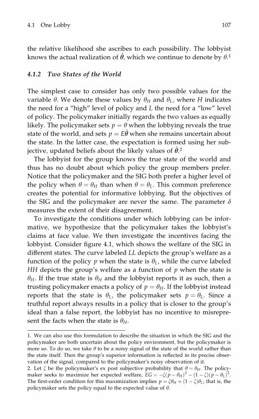
the relative likelihood she ascribes to each possibility. The lobbyist

knows the actual realization of ~yy, which we continue to denote by y.1

4.1.2 Two States of the World

The simplest case to consider has only two possible values for the

variable y. We denote these values by yH and yL, where H indicates

the need for a ‘‘high’’ level of policy and L the need for a ‘‘low’’ level

of policy. The policymaker initially regards the two values as equally

likely. The policymaker sets p ¼ y when the lobbying reveals the true

state of the world, and sets p ¼ E~yy when she remains uncertain about

the state. In the latter case, the expectation is formed using her sub-

jective, updated beliefs about the likely values of ~yy.2

The lobbyist for the group knows the true state of the world and

thus has no doubt about which policy the group members prefer.

Notice that the policymaker and the SIG both prefer a higher level of

the policy when y ¼ yH than when y ¼ yL. This common preference

creates the potential for informative lobbying. But the objectives of

the SIG and the policymaker are never the same. The parameter d

measures the extent of their disagreement.

To investigate the conditions under which lobbying can be infor-

mative, we hypothesize that the policymaker takes the lobbyist’s

claims at face value. We then investigate the incentives facing the

lobbyist. Consider figure 4.1, which shows the welfare of the SIG in

different states. The curve labeled LL depicts the group’s welfare as a

function of the policy p when the state is yL, while the curve labeled

HH depicts the group’s welfare as a function of p when the state is

yH . If the true state is yH and the lobbyist reports it as such, then a

trusting policymaker enacts a policy of p ¼ yH . If the lobbyist instead

reports that the state is yL, the policymaker sets p ¼ yL. Since a

truthful report always results in a policy that is closer to the group’s

ideal than a false report, the lobbyist has no incentive to misrepre-

sent the facts when the state is yH.

1. We can also use this formulation to describe the situation in which the SIG and thepolicymaker are both uncertain about the policy environment, but the policymaker ismore so. To do so, we take y to be a noisy signal of the state of the world rather thanthe state itself. Then the group’s superior information is reflected in its precise obser-vation of the signal, compared to the policymaker’s noisy observation of it.2. Let z be the policymaker’s ex post subjective probability that y ¼ yH . The policy-maker seeks to maximize her expected welfare, EG ¼ �zðp� yHÞ2 � ð1� zÞðp� yLÞ2.The first-order condition for this maximization implies p ¼ zyH þ ð1� zÞyL; that is, thepolicymaker sets the policy equal to the expected value of y.

4.1 One Lobby 107

If the state instead is yL, a truthful (and trusted) report by the

lobbyist induces a policy of p ¼ yL. This is smaller than the group’s

ideal policy of yL þ d in state yL. If the lobbyist instead claims that the

state is yH , the policy outcome will be p ¼ yH . The SIG members may

prefer this larger policy, but it also might be too large even for their

tastes. The lobbyist will report truthfully in state yL if and only if

the SIG members prefer p ¼ yL to p ¼ yH; that is, if and only if

ðyL þ dÞ � yL a yH � ðyL þ dÞ. Notice that this inequality is satisfied

for the case depicted in figure 4.1

We can rewrite the inequality as a limitation on the size of the

divergence in preferences; that is,

dayH � yL

2: ð4:1Þ

When (4.1) is satisfied, there exists an equilibrium with informative

lobbying.3 In such an equilibrium, the lobbyist educates the policy-

Figure 4.1

Example with Two States

3. Game theorists have developed the notion of a Bayesian equilibrium to describeoutcomes of games with imperfect information, and the notion of a perfect Bayesianequilibrium (PBE) to select among such equilibria. In an equilibrium, beliefs areupdated according to Bayes’ rule, all strategies must be best responses to the strategiesof rivals, and they have to satisfy subgame perfection. The latter means that playerscorrectly anticipate subsequent incentives facing their rivals at every stage of thegame. Moreover, a PBE requires that players update their beliefs using Bayes’ ruleeven out of equilibrium, whenever that is possible. See Fudenberg and Tirole (1991,Chapter 6). In the equilibrium with truthful revelation that exists when condition (4.1)is satisfied, the policymaker updates her beliefs based on the report of the SIG. Theupdating causes the policymaker to attach a probability of one to the event that thestate of nature is yH when the SIG reports it as such, and similarly for yL. This is con-sistent with Bayes’ rule in the indicated equilibrium.

108 Lobbying

maker about the state of the world. The equilibrium that results is

‘‘fully revealing,’’ because the policymaker learns the true state for all

possible values of the random variable ~yy.

If, in contrast, (4.1) is not satisfied, the lobbyist’s report lacks

credibility. The policymaker would know in such circumstances that

the lobbyist had an incentive to announce the state as yH no matter

what the true state happened to be. For this reason, his report is

uninformative, and the policymaker is well justified in ignoring its

content. In the event, the policymaker sets the policy p ¼ ðyL þ yHÞ=2that matches her prior expectation about the mean value of ~yy. Evi-

dently, the transmission of information via lobbying requires a suffi-

cient degree of alignment between the interests of the policymaker

and the interest group.

Now let us return to the case in which inequality (4.1) is satisfied.

We have identified an equilibrium with informative lobbying. But

that is not the only possible outcome. Indeed, there is another equi-

librium in which the lobbying effort fails. To see that this is so, sup-

pose the policymaker distrusted the lobbyist. Then she would invoke

the policy p ¼ ðyL þ yHÞ=2 no matter what report she heard. Antici-

pating this behavior, the lobbyist would have no incentive to report

truthfully. For any parameter values, there is an equilibrium out-

come in which the policymaker remains uninformed. Game theorists

refer to this as a ‘‘babbling equilibrium,’’ for it is as if the lobbyist

babbles when providing his report.

Although the babbling equilibrium always exists, Farrell (1993)

has argued that it is not always a reasonable prediction of what may

happen in a cheap-talk game. He has proposed a stricter concept of

equilibrium that sometimes rules out the uninformative outcome.

Farrell’s refinement is based on the idea of a supporting argument.

That is, he would allow the lobbyist to accompany his report of y

with a short supporting speech. Like the report, the arguments in

the speech would not be verifiable by the policymaker. But if they

are nonetheless compelling, the policymaker might take them into

account. Farrell suggests that a plausible equilibrium should be

immune to speeches of the sort he describes.

To pursue this idea for a moment, suppose the lobbyist senses the

policymaker’s distrust. Let the true state be yL, so that the lobbyist

anticipates a policy of p ¼ ðyL þ yHÞ=2 unless he can make his case.

Now imagine that he utters the following speech:

4.1 One Lobby 109

‘‘Please believe me that the state is yL. You should believe me,

because I would have no incentive to make this speech and have

you believe me were the true state to be yH.’’

As figure 4.1 shows, yL is farther from yH þ d than is ðyL þ yHÞ=2.So the lobbyist’s claim that he would not wish to make the speech

in state yH indeed is compelling. Now we must ask whether the

lobbyist would be inclined to make the speech in state yL. If he did so

and succeeded in convincing the policymaker, the policy outcome

would be p ¼ yL. The SIG prefers this outcome to p ¼ ðyL þ yHÞ=2if and only if d < ðyH � yLÞ=4. Thus, Farrell would argue that the

babbling equilibrium is implausible for small values of d, that is, for

d < ðyH � yLÞ=4.4Farrell offers an interesting refinement of the equilibrium concept

for cheap-talk games. But his proposal and others like it remain

controversial.5 Indeed, there are no equilibrium refinements that

command universal support. Since it is not our aim to make strong

predictions about policy outcomes, we do not take a position on

which refinements are most plausible, nor do we devote much space

to them in what follows.

4.1.3 Three States of the World

Now suppose there are three possible states of the policy environ-

ment. The possible values of ~yy are yL, yM, and yH , with yL < yM < yH .

Again, let the policymaker perceive the three states as equally likely.

We ask: When can the lobbyist advise the policymaker of the true

state?

Again, we begin by hypothesizing that the lobbyist’s report will be

taken at face value. Then, a report of yL induces a policy of yL, a

report of yM induces a policy of yM, and a report of yH induces a

policy of yH . Consider first the incentives for false reporting in state

yL. The lobbyist has two possible false reports. He could exaggerate

4. Note that if d < ðyH � yLÞ=4, it is always in the group’s interest, and always credible,for the lobbyist to make the analogous speech about state yH : If y ¼ yH , the SIG prefersthe outcome p ¼ yH to p ¼ ðyL þ yHÞ=2, whereas if y ¼ yL, the SIG prefers p ¼ðyL þ yHÞ=2 to p ¼ yH .5. Farrell’s proposed refinement has been criticized for its implicit assumption that thelistener draws no inference from the lobbyist’s failure to provide a supporting argu-ment. See Farrell and Rabin (1996) for further discussion of equilibrium refinements incheap-talk games.

110 Lobbying

his claim modestly and report the state as yM. Or he could exaggerate

it dramatically and report the state as yH . The lobbyist prefers to

report truthfully in state yL than to claim the state is yM if and only if

the group’s ideal point, yL þ d, is no closer to yM than it is to yL; that

is, if and only if

dayM � yL

2: ð4:2Þ

As for a false report of yH in state yL, this will be unattractive to the

lobbyist anytime it is unattractive to report the state as yM. When

(4.2) is satisfied, the SIG regards a policy level of yM as too high.

Then, since yH > yM, it must consider a policy level of yH to be

excessive as well.

Now consider the incentives for false reporting in state yM. The

lobbyist has no incentive to report the state as yL when actually it is

yM. After all, the SIG prefers a policy larger than yM, and the false

report would induce the policymaker to choose one that is smaller

than p ¼ yM, which is what she would choose upon hearing a truth-

ful report. But the lobbyist might be tempted to exaggerate, because

by alleging the state to be yH when actually it is yM, he induces a

higher level of the policy variable than otherwise. The lobbyist is

willing to eschew this temptation and report truthfully in state yM if

and only if

dayH � yM

2: ð4:3Þ

This inequality constitutes a second requirement for the existence of

an equilibrium with full revelation.

Finally, consider the incentives for false reporting in state yH. In

this state, the lobbyist has no incentive to report either that the state

is yL or that it is yM. Each of these false reports would result in a

policy level that is lower than p ¼ yH. And the group regards even

this policy level to be less than what it desires. Thus, there is no

additional restriction needed for truthful reporting in state yH .

The inequalities (4.2) and (4.3) constitute necessary and sufficient

conditions for an equilibrium with truthful reporting. Notice that, by

introducing a third possible value of ~yy, we have added another re-

striction on the extent of disagreement between the policymaker and

the interest group that is consistent with fully informative lobbying.

4.1 One Lobby 111

Now suppose that one of the conditions (4.2) or (4.3) is violated. Is

the lobbyist bound to babble? Or might he be able to communicate

some more-limited information to the policymaker? In fact, limited

communication may still be possible, as Crawford and Sobel (1982)

have emphasized in their seminal article on strategic information

transmission.

Take, for example, the case in which inequality (4.3) is violated.

The temptation to exaggerate in state yM precludes the lobbyist from

revealing whether the state is ‘‘medium’’ or ‘‘high.’’ But the lobbyist

may nonetheless be able to distinguish this pair of states from one

that requires a low level of the policy instrument. Suppose the

lobbyist were to issue one of two possible reports, with the aim

of making this lesser distinction. Specifically, let a report of ‘‘low’’

indicate that the state is yL and a report of ‘‘not low’’ indicate that the

state is either yM or yH . Then a policymaker who takes the lobbyist’s

claims at face value sets p ¼ yL when she hears that the state is ‘‘low’’

and p ¼ ðyM þ yHÞ=2 when she hears otherwise. The latter policy

level matches her expectation of the state of the world in situations in

which she can rule out the possibility that y ¼ yL but remains other-

wise uninformed. We now must ask again whether the lobbyist has

an incentive to report falsely in any of the three states.

Clearly, the lobbyist has no incentive to do so when the true state

is yH . A false claim of ‘‘low’’ would induce a policy of p ¼ yL.

This outcome is less desirable to the group than the policy p ¼ðyM þ yHÞ=2 that results from a truthful report of ‘‘not low.’’ When

the state is yM, the lobbyist also confronts a choice between the out-

comes p ¼ ðyM þ yHÞ=2 and p ¼ yL. A truthful report of ‘‘not low’’

yields the former level of policy, whereas a false report yields the

latter. The lobbyist will not report falsely if and only if the former

policy is at least as close to the group’s ideal of yM þ d than the latter,

that is, if and only if ðyM þ dÞ � yL b ðyM þ yHÞ=2� ðyM þ dÞ or

dbyH � yM

4� yM � yL

2: ð4:4Þ

Notice that condition (4.4) must be satisfied when (4.3) is violated.

So, truthful reporting in state yM is not an issue in situations in which

the lobbyist cannot credibly distinguish between yM and yH.

Finally, we must check that the lobbyist has no incentive to report

falsely when the state is yL. In this state, a truthful report results in a

policy of p ¼ yL, whereas a false report leads to p ¼ ðyM þ yHÞ=2. The

112 Lobbying

group prefers the former outcome if and only if ðyL þ dÞ � yL a

ðyM þ yHÞ=2� ðyL þ dÞ, or

dayH � yM

4þ yM � yL

2: ð4:5Þ

When conditions (4.4) and (4.5) are satisfied, there exists an equi-

librium with partial transmission of the interest group’s knowledge.

It is easy to check that (4.4) and (4.5) can be satisfied when one of

(4.2) and (4.3) is violated. Suppose, for example, that yL ¼ 0, yM ¼ 4,

and yH ¼ 6. Then (4.3) requires da 1, whereas (4.5) requires only

that da 5=2. For 1 < da 5=2, the lobbyist can credibly distinguish

between a low state and others, but cannot advise the policymaker

whether the state is ‘‘medium’’ or ‘‘high.’’

Suppose now that conditions (4.2) and (4.3) are satisfied, and that

(4.4) and (4.5) are satisfied as well.6 In such circumstances, there

exists an equilibrium in which the lobbyist reports the precise state of

the world and another equilibrium in which he (sometimes) issues a

coarser report. Moreover, a third equilibrium exists in which the

lobbyist babbles. Each of these reporting strategies can be justified by

consistent beliefs of the policymaker. But note that the policymaker

fares best in the fully revealing equilibrium.7 So too does the SIG, at

least in an ex ante sense.8 The lobbyist and the policymaker might

coordinate on this equilibrium, if each expects the other to use the

language that affords both the highest ex ante welfare.

4.1.4 Continuous Information

As the number of possible states grows, full revelation becomes ever

more difficult to achieve. For a lobbyist to be able to distinguish

among all possible states, d must be smaller than one-half of the dis-

6. When yL ¼ 0, yM ¼ 4 and yH ¼ 6, for example, (4.2), (4.3), (4.4), and (4.5) are sat-isfied for all da 1.7. Expected welfare for the policymaker is � 2

9 ½ðyH � yMÞ2 þ ðyM � yLÞðyH � yLÞ� in thebabbling equilibrium, � 1

6 ðyH � yMÞ2 in the equilibrium with partial revelation, and 0 inthe equilibrium with full revelation. Thus, the policymaker’s expected welfareincreases with the level of detail in the lobbyist’s report.8. By ex ante welfare, we mean the expected welfare of the group as viewed from atime before it learns the state of the world. Ex ante welfare is calculated using theprior distribution for ~yy. We find that EU ¼ �d2 � 2

9 ½ðyH � yMÞ2 þ ðyM � yLÞðyH � yLÞ�in the babbling equilibrium, EU ¼ �d2 � 1

6 ðyH � yMÞ2 in the equilibrium with partialrevelation, and EU ¼ �d2 in the equilibrium with full revelation. So the group’s exante ordering of the equilibria is the same as that of the policymaker.

4.1 One Lobby 113

tance between any two of them. But as the number of states tends to

infinity—as it must, for example, when y represents a continuous

variable—this requirement becomes impossible to fulfill. An interest

group that has information about a continuous variable can never

communicate to the policymaker the fine details of its knowledge.

The reason for this should be clear by now. Consider two possi-

ble values of a policy-relevant variable that are close to one another.

For example, the cost of building a school might be either $100 per

square foot or $101 per square foot. A lobbyist for the teachers’ union

realizes that the policymaker will opt for a larger school if she learns

that costs are lower. If the union members value space in the school

more highly than the policymaker, the lobbyist will always be

tempted to report the $100 figure when the actual figure is $101. A

slight understatement of costs would push the policymaker toward a

slightly larger school, but would never result in one being built that

exceeds the teachers’ preferred size. The policymaker cannot trust a

claim that ‘‘costs are $100,’’ even if the SIG has precise information of

this sort.

Although the lobbyist cannot credibly distinguish between cost

figures that are close to one another, it may be possible for him to

advise the policymaker about ranges of costs. Suppose the lobbyist

is expected to report ‘‘low’’ whenever costs fall between $70 and $90

per square foot and to report ‘‘high’’ when they fall between $90

and $110 per square foot. If the policymaker trusts such reports, she

will build a school commensurate with the average cost in the indi-

cated range. But then the lobbyist may have reason to report the

range truthfully, because a misrepresentation when costs are high

could lead to a bill that even the union members would regard as

excessive.

What statements by the lobbyist would be credible in this situa-

tion? To answer this question, we assume that the policymaker’s

prior beliefs are that ~yy is uniformly distributed on the interval

between ymin and ymax. The lobbyist knows y, the realized value of ~yy,

but he does not report a precise figure, because such a report would

not be credible. Instead, he indicates a range that contains the true

value of y. If the lobbyist reports that ‘‘y is in range 1,’’ the policy-

maker interprets this to mean that ymin a ya y1 for some value of y1.

If he reports that ‘‘y is in range 2,’’ the interpretation is that

y1 a ya y2. Let there be n ranges in total, so that the statement ‘‘y is

in range n’’ means that yn�1 a ya yn. We denote the ranges by

114 Lobbying

R1;R2; . . . ;Rn. Our task is to find values of y1; y2; . . . ; yn such that, if

the policymaker takes the lobbyist’s assertions at face value, the

lobbyist has no incentive to lie.

Consider first the statement ‘‘y is in R1.’’ If the policymaker treats

this claim as truthful, she updates her beliefs using Bayes’ rule. Then

her expected value of ~yy is ðymin þ y1Þ=2, and she sets the policy at this

level. We must now check that the SIG prefers the outcome

p ¼ ðymin þ y1Þ=2 for all values of y that are actually in R1 to the

policy levels that would result from false claims of ‘‘y is in R2,’’ ‘‘y is

in R3,’’ and so on. If it does not, then the policymaker should not

trust the lobbyist’s report.

Among values of y in R1, the lobbyist’s greatest temptation to lie

occurs when y actually is close to y1. These highest values of y are

the ones for which the group’s preferred policy is the largest. If the

lobbyist does not wish to exaggerate his claim when y is very close

to y1, he will not wish to do so for smaller values of y. Moreover, if

the lobbyist has no incentive to make the false statement ‘‘y is in R2’’

when ya y1, it is because that claim would generate a policy that

exceeds the group’s preferred policy given the true value of y. Then,

further exaggeration (such as ‘‘y is in R3’’) would generate even

greater overshooting of the group’s desired outcome. It follows that

the only false statement we need investigate is the claim ‘‘y is in R2’’

when actually y is at the upper end of R1.

We now ask, for what values of y1, y2, and d does the SIG prefer to

tell the truth in this situation? A false claim of ‘‘y is in R2’’ causes the

policymaker to update her beliefs so that E~yy ¼ ðy1 þ y2Þ=2. Thus, thefalse claim yields a policy level of p ¼ ðy1 þ y2Þ=2. If the lobbyist is

not tempted to make this false claim when y is a bit less than y1, it

means that this policy level exceeds the group’s ideal of almost y1 þ d

by at least as much as the policy that results from truthful reporting

falls short of this ideal. In symbols, credibility requires ðy1 þ y2Þ=2�ðy1 þ dÞb ðy1 þ dÞ � ðymin þ y1Þ=2, or

y2 b 2y1 þ 4d� ymin: ð4:6Þ

Now suppose that y actually is in R2. There are two things to check

here. First, the lobbyist must not wish to understate the truth (by

claiming that y is in R1) when y is at the lower end of the range.

Second, he must not wish to overstate the truth (by claiming that y is

in R3 or beyond) when y is at the upper end of the range. For values

of y in R2, truthful reporting generates a policy of p ¼ ðy1 þ y2Þ=2. A

4.1 One Lobby 115

false report that y is in R1 would induce a policy of p ¼ ðymin þ y1Þ=2.The SIG prefers the former outcome to the latter when y is near y1 if

and only if ðy1 þ dÞ � ðymin þ y1Þ=2b ðy1 þ y2Þ=2� ðy1 þ dÞ, or

y2 a 2y1 þ 4d� ymin:

Notice that this inequality is the opposite of (4.6). Therefore, both

can be satisfied if and only if

y2 ¼ 2y1 þ 4d� ymin: ð4:7Þ

At the upper end of R2, the temptation is to exaggerate by claiming

that ‘‘y is in R3.’’ By arguments analogous to those above, truthful

reporting when the actual value of y is near y2 requires

y3 b 2y2 þ 4d� y1:

But truthful reporting for values of y at the lower end of R3 requires a

similar inequality running in the opposite direction. So, we need

y3 ¼ 2y2 þ 4d� y1. More generally, a series of requirements for cred-

ibility are that

yj ¼ 2yj�1 þ 4d� yj�2 ð4:8Þ

for all values of j from 2 through n, where y0 ¼ ymin is the initial

condition.

Finally, consider values of y in Rn. Here there is no possibility for

the lobbyist to claim an even higher range for y, because the policy-

maker knows the maximum value in the distribution of ~yy. But then

the topmost value of y in Rn must coincide with the greatest possible

value of ~yy, or

yn ¼ ymax: ð4:9Þ

If values of y1; . . . ; yn can be found that satisfy (4.7), (4.8), and (4.9)

and that have ymin < y1 < y2 < � � � < yn, then these values describe

the credible messages in a lobbying equilibrium. Notice that, if

y1 > ymin and (4.7) is satisfied, this implies y2 > y1. This inequality

and (4.8) ensures y3 > y2. Then y4 > y3, and so on. Therefore, the

procedure for finding an equilibrium is to solve the n linear equa-

tions in (4.8) and (4.9), and then verify that y1 > ymin.

It will not be possible to have an arbitrarily large number of ranges

in a lobbying equilibrium, because information transmission is lim-

ited by the degree of similarity in the interests of the policymaker

116 Lobbying

and the SIG. There must be a largest possible number of ranges that

depends on d and the other parameters. To see how this works, con-

sider an example with ymin ¼ 0 and ymax ¼ 24. Then, if d > 6, the only

equilibrium has n ¼ 1. In this equilibrium, the lobbyist reports that

‘‘y is between ymin and ymax’’ and the policymaker sets p ¼ 12. Of

course, the policymaker learns nothing from such a report, so the

unique outcome is none other than the babbling equilibrium. To see

that informative lobbying is not possible with d > 6, note that equa-

tions (4.8) and (4.9) require, for n ¼ 2, that y1 ¼ 12� 2d and y2 ¼ 24.

But then d > 6 implies y1 < 0, which is impossible because y1 must be

at least as large as ymin. With a large divergence in interests between

the policymaker and the lobbyist, the lobbyist is unable to share any

of his knowledge.

Now suppose instead that d ¼ 4. Then the lobbyist can credibly

claim that ‘‘y is in the range from 0 to 4’’ or ‘‘y is in the range from 4

to 24.’’ In this case, when y actually is a bit less than 4, a truthful re-

port induces a policy of p ¼ 2, which falls short of the group’s ideal

by a bit less than 6. A false report induces p ¼ 14, which exceeds the

group’s ideal by a bit more than 6. So, the lobbyist has no incentive

to claim that ‘‘y is in R2’’ when actually it is in R1. And when the

actual value of y is a bit more than 4, the lobbyist similarly has no

incentive to claim that ‘‘y is in R1.’’ In this case, a lobbying equilib-

rium exists with two alternative reports. We shall refer to this as a

2-partition equilibrium.

It is possible to derive an explicit solution for yj from (4.8) and

(4.9).9 It will be useful to have this solution for some of our later

discussions. We note that (4.8) and (4.9) are satisfied when

yj ¼j

n

� �ymax þ

n� j

n

� �ymin � 2 jðn� jÞd ð4:10Þ

for all values of j between 1 and n. An equilibrium further requires

that y1 > ymin. By applying the formula in (4.10) with j ¼ 1, we see

that y1 > ymin if and only if

2nðn� 1Þd < ymax � ymin: ð4:11Þ

Inequality (4.11) is a necessary and sufficient condition for the

existence of a lobbying equilibrium with n different reports. By

9. Equation (4.8) constitutes a second-order, linear difference equation for yj, whichmust be solved subject to the initial condition, y0 ¼ ymin, and the terminal condition,yn ¼ ymax.

4.1 One Lobby 117

inspecting this inequality, we can draw the following conclusions.

First, an equilibrium with n ¼ 1 always exists; this is the babbling

equilibrium. Second, if an equilibrium with n reports exists, then an

equilibrium with k reports also exists, for all k < n. This follows from

the fact that the left-hand side of the inequality increases with n, so

that if the inequality is satisfied for some integer n, it will also be

satisfied for all smaller integers. Finally, the smaller is d, the larger is

the maximum number of feasible partitions. This confirms our intu-

ition that the prospects for information transmission improve when

the preferences of the SIG and the policymaker become more similar.

4.1.5 Ex Ante Welfare

We have seen by now that more than one equilibrium may exist in

the lobbying game. For example, there always exists a babbling

equilibrium, and if d < ðymax � yminÞ=4, there also exists an informa-

tive equilibrium in which the lobbyist issues one of two possible

reports. Furthermore, if d < ðymax � yminÞ=12, then a 3-partition equi-

librium also exists. Repeated application of equation (4.10) with

n ¼ 4; 5; . . . gives the conditions for the existence of equilibria with

larger numbers of alternative reports.

When several different partition equilibria exist for a given set of

parameter values, it is impossible to say definitively which one will

emerge. All of the equilibria are self-sustaining, in the sense that if

the policymaker expects the lobbyist to issue one of k reports, then

the lobbyist can do no better than to behave as expected. And there is

little to pin down the policymaker’s beliefs. Thus, we are left with an

inevitable ambiguity in the model’s prediction.

In some circumstances, however, the policymaker and the lobbyist

might be able to coordinate on a particular equilibrium. This is most

likely to be true if the two sides agree on their rankings of the alter-

native equilibria. We consider the rankings from an ex ante perspec-

tive; that is, before the play of the game. For the policymaker, an

ex ante perspective means that she evaluates her expected welfare

using her prior beliefs about the distribution of ~yy. As for the interest

group, we have assumed of course that it knows or learns the true

value of y. But we still may be able to evaluate the group’s ex ante

welfare if we can imagine a time before the group gains that knowl-

edge. At such a time, the SIG, like the policymaker, may regard all

values of y between ymin and ymax as equally likely.

118 Lobbying

To see if the policymaker and the SIG concur in their ex ante

rankings, we first calculate the expected welfare of the policymaker.

Recall that the policymaker has the objective function G ¼ �ðp� yÞ2.She expects to learn which of the n ranges contains the actual value

of y, and to set the policy p ¼ ðyj�1 þ yjÞ=2 when she learns that y is in

Rj. Taking all possible realizations of ~yy into account, her expected

welfare in an n-partition equilibrium is10

EGn ¼ � 1

12ðymax � yminÞXn

j¼1

ðyj � yj�1Þ3: ð4:12Þ

Now we calculate the expected welfare of the interest group.

Again, the expectation is taken with respect to the group’s prior

beliefs about the likelihood of the different possible values of y.

We assume that the group has uniform prior beliefs. Its ex ante

expected welfare in an n-partition equilibrium is calculated using

U ¼ �ðp� y� dÞ2 and the policies it anticipates being implemented

after each possible realization of ~yy, and is given by

EUn ¼ � 1

12ðymax � yminÞXn

j¼1

ðyj � yj�1Þ3 � d2: ð4:13Þ

Comparing (4.12) and (4.13), we see that the policymaker and the

SIG do agree on their ranking of the possible equilibria. In fact, the

ex ante welfare of the policymaker and the interest group always

differ by the constant amount d2.

We can use (4.12) and (4.13) to identify the ex ante favorite equi-

librium of both sides. Using (4.10), we calculate

�Pn

j¼1ðyj � yj�1Þ3

ymax � ymin¼ �ðymax � yminÞ2

n2� 4d2ðn2 � 1Þ: ð4:14Þ

Since the right-hand side of (4.14) is an increasing function of n for all

values of n that satisfy (4.11), it follows that the ex ante welfare of the

10. We calculate expected utility from

EGn ¼ � 1

ymax � ymin

Xn

j¼1

ð y j

yj�1

y j þ yj�1

2� y

� �2dy:

Here 1=ðymax � yminÞ is the probability density of ~yy and �½ðy j þ yj�1Þ=2� y�2 is thepolicymaker’s utility for a given realization of ~yy in the range Rj. The formula sumsthe utilities for all values of ~yy in each range, sums over all ranges, and adjusts for thelikelihood of each possible value of ~yy.

4.1 One Lobby 119

policymaker and the interest group both increase with n.11 Thus,

both sides would agree, ex ante, that the equilibrium using the

greatest number of different reports is the best among all equilibrium

outcomes.12

4.2 Two Lobbies

So far we have considered a setting in which a single interest group

lobbies the policymaker. But often policymakers are lobbied by more

than one party. Several groups may have information about the

policy environment, and each may try to persuade the policymaker

to take decisions that it considers best. In such circumstances, the

policymaker must weigh the credibility of the various groups and

decide what advice to heed and what to dismiss.

But the problem of information transmission with multiple lobbies

is more subtle than that. The lobbying game between an interest

group and a policymaker is altered by the presence of other lobbies.

A policymaker may be able to play off one information source

against another by asking an informed group to confirm or contra-

dict the reports she has already heard. The lobbyists must consider

more than just their own direct relationship with the policymaker.

Each must realize that the reports of others will affect how their own

messages are interpreted, and that their own reports may alter the

incentives that other groups have when it comes time for them to

advise the policymaker.13

In this section we study a lobbying game with two informed interest

groups. Our discussion draws heavily on Krishna and Morgan

11. Consider the difference between the right-hand side of (4.14) evaluated at n ¼ mand evaluated at n ¼ m� 1. It equals

ð2m� 1Þ ðymax � yminÞ2

m2ðm� 1Þ2� 4d2

" #:

With (4.11) being satisfied for n ¼ m, this expression must be positive.12. It may seem obvious, at first glance, that more reports are better, because infor-mation sharing improves the quality of policy decisions. But the result is not trivial,because when adding more reports, the lobbyist does not simply subdivide some ofthe ranges he would have used in an equilibrium with fewer reports. Rather, theranges in the two different equilibria typically overlap.13. Interest groups may be able to prove that they are telling the truth, or the policy-maker may be able to detect utterly untruthful messages, as in Milgrom and Roberts(1986). Moreover, the policymaker may be able to use one interest group to confirm ordisprove messages from another group, as in Lipman and Seppi (1995). We abstractfrom these interesting variants of the problem.

120 Lobbying

(2001). We follow them in distinguishing two different situations.

In one, which they call the case of ‘‘like bias,’’ the preferences of the

two groups are biased in the same direction relative to those of the

policymaker. That is, for each state of the world, either both groups

prefer a policy p that is larger than what the policymaker would

choose if she knew the true state, or both groups prefer a policy that

is smaller than the policymaker’s ideal choice. The groups may differ

in the extent of their bias, with one group perhaps being more ex-

treme than the other. The issue here is whether the two lobbyists

jointly can communicate more information to the policymaker than

either could convey on his own.

The second case is one of ‘‘opposite bias.’’ In this setting, the

groups’ ideal points for a given state of the world lie on opposite

sides of the policymaker’s ideal. One group prefers a higher policy

level than the politician, while the other prefers a smaller level. This

pits the lobby groups against one another, to the potential advantage

of the policymaker. Again we investigate what the policymaker can

learn and ask whether the lobbyists can guard themselves against

contradictory reports by their political adversaries.

4.2.1 Like Bias

We begin with the case of like bias. As before, the policymaker must

take a decision p with consequences that depend on the state of

the world, y. The policymaker’s objective is to maximize Gðp; yÞ ¼�ðp� yÞ2. She has two potential sources of information about y.

These sources are two lobbyists, each of whom is fully informed

about the policy environment. The lobbyist for SIG 1 seeks to max-

imize U1ðp; yÞ ¼ �ðp� y� d1Þ2, while that for SIG 2 seeks to max-

imize U2ðp; yÞ ¼ �ðp� y� d2Þ2. The case of like bias arises when the

value of p that maximizes Gðp; yÞ is smaller (or larger) than the value

that maximizesU1ðp; yÞ and the one that maximizes U2ðp; yÞ, for everyvalue of y. When, as here, the welfare functions are quadratic, this

case arises when d1 and d2 have the same sign. For concreteness, we

suppose 0 < d1 a d2, so that SIG 1 is (if anything) the more moderate

interest group while SIG 2 is more extreme.

The outcome of the lobbying game may depend on the order in

which the lobbyists meet with the policymaker and on what each

knows about the advice given by the other. We can imagine at least

three different scenarios. First, the meetings between the lobbyists

4.2 Two Lobbies 121

and the policymaker might be a secret, so that each informant is

ignorant of the fact that the policymaker has an alternative informa-

tion source. Second, the meetings between lobbyist and policymaker

might be private, in which case a lobbyist will know that another has

offered advice (or will offer advice) but not the content of the dis-

cussion. Finally, a lobbyist’s recommendation to the policymaker

may become public, in which case subsequent advisers can condition

their reports on the information that the policymaker already has.

We will concentrate our discussion on public messages, but first say

a few words about the other two scenarios.14

Secret Messages

When the lobbyists meet secretly with the policymaker, there can be

no strategic interaction between them.15 Neither lobbyist realizes

that another meeting might take place, and so neither anticipates that

the policymaker has another informant. We cannot really speak of an

equilibrium in this situation, because a lobbyist’s perception of how

the policymaker will respond to his message will not be consistent

with how the policymaker actually responds. Each lobbyist will

behave as if he were the sole provider of information, and so act

according to the prescriptions of one of the equilibria we studied

before. The policymaker, however, will take an action based on the

combined advice of the two lobbyists.

We bring this case up only to point out how the policymaker

might try to combine the information contained in two distinct

reports. Suppose the first lobbyist sends either a message m1, which

the policymaker interprets to mean ya y1, or a message m2, which

the policymaker interprets to mean yb y1. The second lobbyist, not

knowing of the existence of the first, sends either mm1, which means

ya yy1, or mm2, which means yb yy1. Finally, suppose for concreteness

that y1 < yy1. Then, if the policymaker hears the reports m1 and mm1,

she infers ymin a ya y1; these are the only values of ~yy that are con-

sistent with her prior understanding of the distribution of the

14. It is also possible to imagine situations in which, after receiving messages from alobbyist, the policymaker issues statements that reveal some of the information con-tained in these messages. We will not examine such possibilities here.15. This statement is true when the lobbyists do not even conceive of the possibilitythat the policymaker has another source of information. Alternatively, the lobbyistsmay suspect that other secret meetings might take place, in which case they will formexpectations of the likelihood of such meetings and adjust their reports accordingly.The situation then is similar to that of private messages, which we discuss below.

122 Lobbying

random variable and the pair of reports she has received. Similarly,

if the policymaker hears m2 and mm2, she infers yy1 a ya ymax. Finally,

if she hears m2 and mm1, she infers y1 a ya yy1.16 Notice that the pair of

messages convey more information about the true state of the world

than does either message alone. The policymaker can combine the

information contained in two messages to refine her beliefs about the

policy environment

But the very fact that the meaning of a message changes when

combined with another implies that the lobbyists’ incentives change

once each becomes aware of the other’s existence. Consider, for

example, a setting in which the policymaker initially believes that

y lies between 0 and 24, and that all values are equally likely. Sup-

pose that d1 ¼ 1 and d2 ¼ 2. If only the lobbyist for SIG 1 lobbies the

policymaker, there is a 2-partition equilibrium with y1 ¼ 10. In this

case, when the state is y ¼ 10, the lobby is indifferent between the

policy p ¼ 5 that would result from a report of m1 and the policy

p ¼ 17 that would result from one of m2. Each of these policies differs

by 6 from the group’s preferred policy of 11. Similarly, there is a

unique 2-partition equilibrium when the representative of SIG 2

alone lobbies the policymaker. In this equilibrium, the lobbyist

reports mm1 if ya 8 and mm2 if yb 8.

This pair of partitions does not, however, constitute an equilibrium

when each lobby is aware that the other will also be providing in-

formation to the policymaker. If the lobbyist for SIG 1 suspects that a

counterpart will report mm1 when ya 8 and mm2 when yb 8, then his

own report of m1 when y slightly exceeds 10 would lead the

policymaker to believe that y lies between 8 and 10. In the event, the

policymaker would set the policy p ¼ 9. SIG 1 prefers this outcome

to the policy p ¼ 17 that would result from a truthful report of m2.

The messages m1 and m2 no longer are credible.

Private Messages

If the lobbyists realize that the policymaker has an alternative infor-

mation source but have no way of observing the other report, then

many different outcomes are possible in the lobbying game. Among

16. The policymaker might also hear m1 and mm2. However, this pair of messagescannot arise if both lobbyists report truthfully. Since the pair of messages occurs withzero probability ‘‘along an equilibrium path’’ (where the lobbyists have an incentiveto report truthfully), Bayes’ rule places no restriction on the policymaker’s updatedbeliefs.

4.2 Two Lobbies 123

these equilibria is one in which the policymaker gains full informa-

tion. To see that this is so, suppose the policymaker believes that

each group will report the state of the world precisely and truthfully.

She interprets a report of m from the lobbyist for SIG 1 to signify that

y ¼ m. Similarly, she interprets a report mm from the lobbyist for SIG 2

to mean that y ¼ mm. Then among her optimal strategies is one in

which she sets p ¼ minfm; mmg. This is not the only strategy that

maximizes the policymaker’s expected welfare, but as long as each

side reports truthfully (as it must in an equilibrium), the strategy

provides the policymaker with her ideal policy in each state of the

world.17

Now consider the incentives facing the lobbyists when they antic-

ipate that the policymaker will follow the indicated strategy. If SIG 1

believes that its counterpart will report truthfully, this group may as

well report truthfully too. For example, if the true state is y ¼ 5, and

SIG 1 expects mm ¼ 5, then it expects p ¼ 5 for any report it might

make of a state greater than or equal to y ¼ 5. If SIG 1 were instead to

report some m < 5, the policymaker would take its false report at

face value and the policy would be even further from the group’s

ideal. A truthful report by SIG 1 is a best response in this situation.

The same is true for SIG 2. By using each lobbyist’s report to discipline

the other’s, the policymaker gains full information and achieves her

desired outcome in every state.

However, the equilibrium with full revelation seems fragile in

these circumstances. The lobbyist for SIG 1 might believe that there is

a small probability that his counterpart will announce a state larger

than 5 when the true state is y ¼ 5. This belief might reflect the pos-

sibility that the other lobbyist will make an error, or the lobbyist for

SIG 1 might simply be unsure of his counterpart’s intentions. If the

lobbyist for SIG 2 does happen to report something larger than 5,

then the lobbyist for SIG 1 would wish he had done so as well.

Moreover, if the lobbyist for SIG 2 does not report a state larger than

5, there is no harm to SIG 1 if its lobbyist exaggerates his own report.

17. As we noted in footnote 16, Bayes’ rule does not restrict what the policymakermay believe after hearing messages that would not be sent in an equilibrium play ofthe game. The optimal strategy we have described arises when the policymakerbelieves, upon hearing two conflicting reports, that the group reporting the smallervalue of y has reported honestly. With these beliefs, it is optimal for her to setp ¼ minfm; mmg.

124 Lobbying

Given the anticipated behavior of the policymaker, it is a weakly

dominant strategy for each lobbyist to report his own group’s ideal

point in every state. If both lobbies recognize this, neither will report

the true state.

Moreover, if the SIGs anticipate an equilibrium with full revelation

of the state of the world, they may try to air their reports publicly.

Whereas the policymaker achieves her first-best outcome in an equi-

librium with private messages and full revelation, the interest groups

with like biases may not be so happy with the situation. Each group

would like the other to exaggerate the state slightly, and then it

would gladly follow suit. The lobbyist for group 1 might attempt to

publicize a report of, say, m ¼ 5:1 when the true state is y ¼ 5, hoping

that the other lobbyist would back up his false claim.

It might be interesting to consider a game in which each lobbyist

has a choice of whether or not to make his report public. In such a

game, the policymaker would be able to draw inferences about the

state of the world not only from the content of the messages, but also

from the manner in which they were communicated. Moreover, the

policymaker herself might have an incentive to make public what

advice she has been given in some situations. But such a game is

rather complicated. Instead, we turn our attention to situations in

which the lobbyists are free to offer their advice publicly and have no

opportunity to do otherwise.

Public Messages

When the lobbies report their information sequentially and the

second lobbyist can learn what the first has said, full revelation

cannot occur in any equilibrium. To see this, suppose to the contrary

that there is an equilibrium in which the policymaker learns the

precise state of the world from the combined reports of the two

lobbyists. Then the policymaker’s best response would be to set

p ¼ y when she learns that the state is y. But the interest groups both

prefer policies greater than y in state y. Therefore, the first-reporting

lobbyist could misrepresent the state in such a way that, if his coun-

terpart follows suit, the policymaker will believe the state to be some

y 0 > y. It would then be in the interest of the second lobbyist to cor-

roborate the first lobbyist’s (false) report.

Krishna and Morgan (2001) prove that, as in the lobbying game

with a single lobby, every equilibrium with two lobbies can be rep-

4.2 Two Lobbies 125

resented as a partition equilibrium.18 In a partition equilibrium, as

before, the policymaker learns that y lies in one of a finite number of

nonoverlapping ranges. With two lobbies, the policymaker’s infor-

mation comes from the combined evidence in the two reports. For

example, a three-partition equilibrium arises when each lobbyist

divides the set of possible values of y into two (nonidentical) subsets.

To show how partition equilibria can be constructed in a lobbying

game with two SIGs, we analyze further the numerical example

described above. In the example, the policymaker initially believes

that y lies between 0 and 24. She sees each such value as equally

likely. Both interest groups have biases toward higher levels of policy

than the policymaker; specifically, d1 ¼ 1 and d2 ¼ 2.

Suppose that the lobbyist representing SIG 1 reports first, and that

his strategy is to issue one of two messages. If he sends message m1,

the policymaker understands it to mean that ya y1 (for some value

of y1 yet to be determined). If he sends the message m2, the policy-

maker infers yb y1. We hypothesize that y1 is reasonably large, so

that the second lobbyist will wish to distinguish further between

states that are ‘‘very low’’ (those that lie between ymin and some yy1Þand those that are only ‘‘reasonably low’’ (lie between yy1 and y1). The

second lobbyist can make this distinction by choosing among two

messages. The policymaker interprets the message mm1 to mean ya yy1and the message mm2 to mean yb yy1. The resulting partition is

depicted in figure 4.2.

First we consider the optimal response by the policymaker to the

reports she may hear. If she hears m1 and mm1, she infers that y lies

18. Actually, they show that all monotonic equilibria are partition equilibria. A mono-tonic equilibrium is one in which the policy outcome in a higher state is always at leastas large as the outcome in a lower state. This property is guaranteed for the lobbyinggame with one informed party, but it is not guaranteed when there is more than oneinformed party. Krishna and Morgan restrict their attention to monotonic equilibria, aswe will do here.

Figure 4.2

Partitions and Policies with Two Reports

126 Lobbying

between 0 and yy1. By Bayes’ rule, all values in this range remain

equally likely. Therefore, she sets p equal to the expected value of ~yy

in this range, that is, pðm1; mm1Þ ¼ yy1=2. This policy is shown in figure

4.2. By similar reasoning, the pair of messages m1 and mm2 induces

pðm1; mm2Þ ¼ ðyy1 þ y1Þ=2, and the pair of messages m2 and mm2 induces

pðm2; mm2Þ ¼ ðy1 þ 24Þ=2. These policies, too, are shown in the figure.

Next we consider the incentives facing the lobbyist for SIG 2. By

the time he must select a message, he will have heard his counterpart

report either m1 or m2. If the first lobbyist has reported m2, this sig-

nifies to the policymaker that yb y1 > yy1. Then, if the lobbyist for

SIG 2 delivers the message mm2, this provides no new information to

the policymaker. If the lobbyist instead delivers the message mm1, the

policymaker will know that at least one of the reports must be false.

But false reports are not part of any equilibrium. So it must be that

the lobbyist for SIG 2 does not wish to send the message mm1 after

hearing his counterpart report m2.19

In contrast, when the report by the lobbyist for SIG 1 has been m1,

the subsequent report by the second lobbyist does provide additional

information to the policymaker. If the second lobbyist delivers the

message mm1, the policymaker infers that ya yy1, and sets the policy

pðm1; mm1Þ ¼ yy1=2. If he instead reports mm2, the policymaker infers that

yy1 a ya y1, and sets the policy pðm1; mm2Þ ¼ ðyy1 þ y1Þ=2. The lobbyist

for SIG 2 must have no incentive to report falsely for any value of y,

and in particular for those values slightly below and slightly above

yy1. As before, this requires the lobbyist to be indifferent between

reporting mm1 and mm2 when the state actually is yy1. Such indifference

arises when ðyy1 þ d2Þ � pðm1; mm1Þ ¼ pðm1; mm2Þ � ðyy1 þ d2Þ, or, with

d2 ¼ 2,

ðyy1 þ 2Þ � yy1

2¼ yy1 þ y1

2� ðyy1 þ 2Þ:

Rearranging terms, this gives

yy1 ¼y1

2� 4: ð4:15Þ

19. The incentives facing the second lobbyist when his counterpart has alreadyreported m2 depend on what inference the policymaker would draw upon hearingcontradictory reports. Bayes’ rule does not apply and therefore does not restrict thepolicymaker’s beliefs in such an event. Without going into the details, we note thatthere are legitimate beliefs for the policymaker that make it undesirable for the lobby-ist for SIG 2 to report mm1 when yb y1 and the other lobby has reported m2. Thesebeliefs support the equilibrium with truthful reporting by both lobbyists.

4.2 Two Lobbies 127

Finally, we consider the incentives facing the lobbyist for SIG 1. He

must anticipate not only how his message will be interpreted by the

policymaker, but also how it will affect the report of the other lobby.

The lobbyist for SIG 1 must not have an incentive to report falsely in

any state. This requires that, when the state is y1, his group is indif-

ferent between the outcome that would ensue from a report of m1

and the one that would result from a report of m2. From what we

have seen, a report of m1 in state y1 leads the lobbyist for SIG 2 to

report mm2. A report of m2 in state y1 also leads to a report of mm2. Thus,

in equilibrium, the lobbyist for SIG 1 anticipates a report of mm2 by

his counterpart, no matter which message he himself delivers. When

the lobbyist for SIG 1 looks beyond the second lobbying report to

the policy-setting stage, he anticipates a choice of p ¼ ðy1 þ yy1Þ=2 in

response to a report of m1 and p ¼ ðy1 þ 24Þ=2 in response to a report

of m2. SIG 1 is indifferent between these outcomes in state y1 if and

only if ðy1 þ d1Þ � ðy1 þ yy1Þ=2 ¼ ðy1 þ 24Þ=2� ðy1 þ d1Þ, or (with d1 ¼ 1,

and after some rearranging of terms),

y1 ¼ 10þ yy1

2: ð4:16Þ

Equations (4.15) and (4.16) are two linear equations that relate y1and yy1. If both of these equations are satisfied, the lobbyists’ messages

will be credible at every stage. The equations have a unique solution

with y1 ¼ 32=3 and yy1 ¼ 4=3, which is shown in panel a of figure 4.3.

Evidently there is a 3-partition equilibrium in which the lobbyist

for SIG 1 first reports whether y is above or below 32=3 and then

the lobbyist for SIG 2 reports whether y is above or below 4=3. The

policymaker sets the policy at either p ¼ 2=3, p ¼ 18=3, or p ¼ 52=3,

depending on what combination of reports she hears.

Figure 4.3

Equilibrium Partitions When SIG 1 Reports First

128 Lobbying

However, this is not the only 3-partition equilibrium that can arise

when SIG 1 reports first. In constructing the equilibrium, we have

assumed that y1 > yy1, so that the first lobbyist distinguishes ‘‘very

low’’ values of y from values that are ‘‘not so low,’’ and the second

further distinguishes ‘‘very large’’ values of y from those that are

only ‘‘moderately large.’’ It is also possible to construct an equilib-

rium with yy1 > y1. Then the roles of the two lobbyists are reversed.

The procedure for constructing the equilibrium is much the same.

First, we find a state yy1 in which the lobbyist for SIG 2 is indifferent

between reporting mm1 and mm2, given that his counterpart has already

reported m2 (i.e., that y > y1Þ. Then we find a state y1 in which the

lobbyist for SIG 1 is indifferent between reporting m1 and m2, in the

light of the equilibrium responses he anticipates. The equations that

are analogous to (4.15) and (4.16) are yy1 ¼ y1=2þ 8 and y1 ¼ yy1=2� 2.

They imply y1 ¼ 8=3 and yy1 ¼ 28=3. These partitions are depicted in

panel b of figure 4.3.

So far we have assumed that the lobbyist for SIG 1 delivers his

message first. We can also consider the game that arises when the

order of reporting is reversed. Also in this game, there are two pos-

sible 3-partition equilibria, one with y1 > yy1 and the other with

yy1 > y1. The procedure for constructing them is the same as before.

It turns out that the equilibrium values for y1 and yy1 are the same as

when SIG 1 reports first; namely, y1 ¼ 32=3 and yy1 ¼ 4=3, or y1 ¼ 8=3

and yy1 ¼ 28=3. The possible policy outcomes also are the same.

Now let us turn our attention from the specific example with

d1 ¼ 1, d2 ¼ 2, and ymax � ymin ¼ 24 to the more general case of like

bias. Krishna and Morgan (2001) have shown that, generally, it does

not matter which lobby group reports first. The sets of possible

equilibria are the same with either sequence of lobbying. Moreover,

for any given set of parameter values, there is a maximum number of

subsets in an equilibrium partition. This number rises (or remains the

same) as either d1 or d2 approaches zero. In other words, the more

similar are the interests of the interest groups and the policymaker,

the more detailed can be the information they convey.

Krishna and Morgan also compare the equilibria that can arise

when two groups lobby the policymaker to those that are possible

when there is only a single lobbyist. They ask whether the addition

of a second lobby improves the prospect for transfer of knowledge.

Their answer is that it does not. In particular, they prove that the

maximum number of subsets in an equilibrium partition with two

4.2 Two Lobbies 129

Bing

高亮

Bing

高亮

Bing

高亮

lobbies of like bias cannot exceed the maximum number of subsets in

an equilibrium partition when only the more moderate of the two

lobbies the policymaker. Moreover, the ex ante welfare of the policy-

maker and of each of the two SIGs is higher in an n-partition equi-

librium with reports by only the more moderate of the two lobbies

than in any n-partition equilibrium in which both lobbies offer their

advice. Therefore, all parties would agree ahead of time (i.e., before y

is known to the SIGs) to have only the more moderate interest group

advise the policymaker rather than to have both groups file reports.

The more moderate group has greater credibility than the other, and

thus is better able to communicate with the policymaker.

4.2.2 Opposite Bias

When interest groups share the same direction of policy bias relative

to a policymaker, it is difficult for the policymaker to use one group

to discipline the statements of others. If one lobbyist misrepresents

the policy environment slightly, the others are happy to corroborate

his report. A policymaker then must rely on keeping her conversa-

tions private in order to elicit truthful confirmation or contradiction

of the reports she hears. But such privacy may be difficult to main-

tain, because the groups have good reasons to publicize their claims.

A policymaker can, however, use competing information sources

to her advantage when lobbies have conflicting policy aims. In such

a setting, if one lobbyist attempts to exaggerate his claims, another

may have an incentive to bring the falsehood to light. Still, as Krishna

and Morgan (2001) have shown, a policymaker can never become

fully informed, even if the lobbyists do represent opposing interests.

To see why, we examine a situation in which d1 < 0, d2 > 0 and the

lobbyist for SIG 1 reports first. We define y�2 1 ymax � d2; that is, y

�2 is

the state of the world in which the ideal policy for SIG 2 is equal to

ymax. Our argument shall be that no equilibrium of the lobbying

game can reveal the precise state of the world for values of y > y�2 .

Suppose, to the contrary, that the policymaker does learn the true

state for such values of y. Consider two states, y 0 and y 00, such that

y 0 > y 00 > y�2 . When the lobbying reveals the state to be y 0, the

policymaker sets the policy p ¼ y 0. When it reveals the state to be y 00,

she sets p ¼ y 00. We take y 0 and y 00 to be sufficiently close together,

so that SIG 1 prefers the policy p ¼ y 00 in state y 0 to the policy p ¼ y 0.

This requires y 0 � y 00 < �d1.

130 Lobbying

Bing

高亮

Let m 0 denote the message that the lobbyist for SIG 1 delivers in

state y 0 and m 00 denote the message he delivers in state y 00. Also, let

mmðmjyÞ denote the optimal response by the lobbyist for SIG 2 to a

message m sent by his counterpart, when the true state is y. Then, in

the hypothesized equilibrium, the lobbyist for SIG 2 reports mm 0 ¼mmðm 0jy 0Þ in state y 0 and mm 00 ¼ mmðm 00jy 00Þ in state y 00, and the policy-

maker responds with pðm 0; mm 0Þ ¼ y 0 and pðm 00; mm 00Þ ¼ y 00 in these states.

We now proceed to establish that these cannot be optimal

strategies for both lobbyists. To begin, suppose that the lobbyist

for SIG 1 were to report m 00 in state y 0, instead of m 0. Then the

response by the second lobbyist would be mmðm 00jy 0Þ. It must be that

p½m 00; mmðm 00jy 0Þ�b y 00, because the lobbyist for SIG 2 could have

responded with mm 00, in which case the policymaker would have

delivered the policy y 00. So the optimal response must leave

SIG 2 at least as well off as this. Furthermore, it cannot be that

p½m 00; mmðm 00jy 0Þ� ¼ y 00, for if it were, SIG 1 would benefit from the

proposed deviation. It follows that p½m 00; mmðm 00jy 0Þ� > y 00. However,

this implies that it is not optimal for the lobbyist for SIG 2 to report

mm 00 in state y 00. He could instead report mmðm 00jy 0Þ and thereby induce a

policy that his group prefers to the outcome p ¼ y 00, which results

when he follows the allegedly optimal strategy. Thus, the assump-

tion of full revelation for states y > y�2 leads to a contradiction.

Although the policymaker cannot gain a complete understanding

of the policy environment from two opposing lobbies, she can learn

more from the two together than from either one alone. To see this,

we pursue another numerical example, this time with d1 ¼ �3 and

d2 ¼ 3. We again take y to lie between 0 and 24. Then, were only SIG

1 to lobby the policymaker, the outcome would either be a babbling

equilibrium or a 2-partition equilibrium. In the latter equilibrium, the

lobbyist for the group sends one message if ya 18 and another if

yb 18. And if only SIG 2 were to lobby, again the outcome would

either be a babbling equilibrium or a 2-partition equilibrium. The

lobbyist’s messages would distinguish between states with ya 6 and

those with yb 6. The reader may confirm that no 3-partition equi-

librium is possible in either of these cases. We now proceed to show

that a 3-partition equilibrium can arise when both groups lobby the

policymaker.

Suppose the lobbyist for SIG 1 reports first, and that he delivers

either message m1 that indicates ya y1 or m2 that indicates yb y1.

The lobbyist renders his advice with the understanding that an

4.2 Two Lobbies 131

opposing group will report subsequently. When it is time for the

lobbyist for SIG 2 to meet with the policymaker, he delivers the

message mm1 that indicates ya yy1 or the message mm2 that means

yb yy1. Our job is to find values of y1 and yy1 such that both reports

are credible when each lobbyist correctly forecasts the ensuing events.

Once the lobbyist for SIG 1 has delivered his message m1, the re-

port by the representative of SIG 2 gives additional information to

the policymaker. Suppose, for example, that y1 b yy1. Then a message

mm1 suggests to the policymaker that y lies between 0 and yy1, while

the message mm2 suggests that y lies between yy1 and y1. With the

former message, the policymaker sets the policy p ¼ yy1=2; with the

latter message, she sets p ¼ ðyy1 þ y1Þ=2. SIG 2 must be indifferent

between these two outcomes when y ¼ yy1, which requires ðyy1 þ 3Þ�yy1=2 ¼ ðy1 þ yy1Þ=2� ðyy1 þ 3Þ, or

yy1 ¼y1

2� 6: ð4:17Þ

Also, the lobbyist for SIG 1 must be indifferent between reporting

m1 and reporting m2 when the state is y1. Since this lobbyist reports

first, he must forecast the response by his counterpart. A report of

m1, coupled with the best response by SIG 2, induces a policy of

p ¼ ðyy1 þ y1Þ=2. A report of m2 and the best response of SIG 2 yields a

policy of p ¼ ðy1 þ 24Þ=2. SIG 1 is indifferent between these two out-

comes in state y1 if and only if ðy1 � 3Þ � ðy1 þ yy1Þ=2 ¼ ðy1 þ 24Þ=2�ðy1 � 3Þ, or

y1 ¼yy1

2þ 18: ð4:18Þ

Equations (4.17) and (4.18) are the only two requirements for a

3-partition equilibrium. They are both satisfied when y1 ¼ 20 and

yy1 ¼ 4. Thus, we have identified a 3-partition equilibrium in which

the lobbyist for the group that prefers a relatively low level of the

policy variable first reports whether y is greater or less than 20, and

the lobbyist for the group that prefers a relatively high level of the

policy subsequently reports whether y is greater than or less than 4.

If the policymaker hears the pair of messages m1 and mm1, she sets

p ¼ 2; if she hears m1 and mm2, she sets p ¼ 12; and if she hears m2 and

mm2, she sets p ¼ 22. These responses validate the lobbyists’ reporting

strategies.

When we compare the expected welfare of the policymaker in the

3-partition equilibrium to what she can achieve when she has only a

132 Lobbying

single source of information, we find that having advisers on opposite

sides of the issue works to the policymaker’s benefit. What is more

surprising, perhaps, is that the groups themselves gain from this, at

least in an ex ante sense. Viewed from a time before the groups learn

the value of y, each has higher expected welfare in the 3-partition

equilibrium that exists when both lobby than in the best equilibrium

that can arise when only one group engages in lobbying. The expla-

nation for this is simple. When a group provides information without

any foil, the policymaker will be wary of its report. This wariness

causes the policy outcome to differ greatly from what is warranted in

some states of the world. But when a group’s report must be con-

firmed by the report of another group that has an opposing bias, the

report enjoys greater credibility. Both groups benefit from the ability

to communicate information about the policy environment.

We have constructed a 3-partition equilibrium for our numerical

example. But this is not the best that can be achieved. In fact, our

example admits equilibria in which the policymaker becomes fully

informed about the policy environment for a range of values of y.

Only for extreme values of the state variable is the policymaker

forced to rely on coarse information.

Krishna and Morgan (2001) show that the properties of our

numerical example are rather general. For the case of opposite bias,

they establish the existence of an equilibrium with ‘‘partial revela-

tion’’ whenever both lobby groups are ‘‘nonextreme.’’ By partial rev-

elation, we mean that lobbying enables the policymaker to infer the

state of the world for a continuous range of values of y. A group is

nonextreme if it does not wish to have the policymaker believe that

the state is ymin (or ymax) in all states of the world. When a partial-

revelation equilibrium does exist, it yields higher ex ante welfare to

the policymaker and to both SIGs than does any equilibrium with

lobbying by only a single group. When a partial-revelation equilib-

rium does not exist, then the groups’ extreme preferences deprive

their lobbyists of any credibility. The only equilibrium in such cir-

cumstances is a babbling equilibrium.

4.2.3 Multidimensional Information

Our discussion in this chapter has been confined to unidimensional

policy issues and unidimensional uncertainty about the policy envi-

ronment. Although much of the literature focuses on this case, that

focus may be limiting. Indeed, a recent paper by Battaglini (2000) has

4.2 Two Lobbies 133

shown that increasing the dimensionality of the policy problem may

improve the prospects for information transmission. That is, lobby

groups may be more effective in communicating information when

there are many dimensions to policy than when the policy choice

concerns the height of a single policy instrument.

We consider now a setting with two interest groups, two dimen-

sions of policy, and two dimensions of policy uncertainty. The two

policy dimensions might reflect different aspects of a single instru-

ment (e.g., the tax rate on long-term capital gains and the minimum

holding period for a gain to be considered ‘‘long term’’), or two

entirely different instruments (e.g., the tax rate on gasoline sales and

the maximum allowable pollution emission). We represent the policy

by a two-dimensional vector p ¼ ðp1; p2Þ and the state of the world

by a two-dimensional vector y ¼ ðy1; y2Þ.20 The welfare function of

the policymaker is Gðp; yÞ ¼ �P2

j¼1ðpj � yjÞ2, while that of SIG i is

Uiðp; yÞ ¼ �P2

j¼1ðpj � yj � dijÞ2, for i ¼ 1; 2. Thus, p ¼ y is the policy-

maker’s ideal policy vector in state of the world y, whereas p ¼ y þ diis the favorite of SIG i in that state. The vector di ¼ ðdi1; di2Þ denotesthe bias in the preferences of SIG i relative to those of the policy-

maker. A group may prefer larger (or smaller) values of p1 and p2than the policymaker in every state of the world, or it may prefer a

larger value on one dimension and a smaller value on the other.

We assume that both groups know the values of both bits of infor-

mation; that is, each knows the realization of the (two-dimensional)

random variable ~yy. Lobbyists for the two groups meet with the poli-

cymaker privately to deliver their assessment of the policy environ-

ment.21 The policymaker uses the advice to update her beliefs about

20. We alert the reader to a temporary change of notation. Whereas until now we haveused y1 to denote the highest value of y for which the lobbyist for SIG 1 sends themessage m1, we now use it to denote the first element of the vector y. We will revert tothe previous usage in the next chapter.21. Recall from Section 4.2.1 that, with like bias and private reporting, there alwaysexists an equilibrium with full revelation. This equilibrium arises when each lobbyistreports a state of the world and the policymaker sets the policy equal to the minimumof the two reports. However, we noted at the time the fragility of this equilibrium. Itrelies on each lobbyist being fully confident that the other will reveal the true state,so that each is indifferent between doing so himself or not. With even the slightestpossibility that a lobby may observe the state of the world with error, the equilibriumwith full revelation disappears. In contrast, the equilibrium with full revelation thatwe shall describe for the case of multiple policy dimensions is immune to this critique,as we shall discuss further below. Battaglini (2000) has shown that full revelationtypically is not possible with sequential public reporting about multiple dimensionsof policy uncertainty unless a special condition relating the groups’ preferences issatisfied.

134 Lobbying

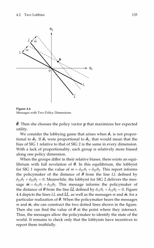
~yy. Then she chooses the policy vector p that maximizes her expected

utility.

We consider the lobbying game that arises when d1 is not propor-

tional to d2. If d1 were proportional to d2, that would mean that the

bias of SIG 1 relative to that of SIG 2 is the same in every dimension.

With a lack of proportionality, each group is relatively more biased

along one policy dimension.

When the groups differ in their relative biases, there exists an equi-

librium with full revelation of y. In this equilibrium, the lobbyist

for SIG 1 reports the value of m ¼ d21y1 þ d22y2. This report informs

the policymaker of the distance of y from the line LL defined by

d21y1 þ d22y2 ¼ 0. Meanwhile, the lobbyist for SIG 2 delivers the mes-

sage mm ¼ d11y1 þ d12y2. This message informs the policymaker of

the distance of y from the line LLLL defined by d11y1 þ d12y2 ¼ 0. Figure

4.4 depicts the lines LL and LLLL, as well as the messages m and mm, for a

particular realization of y. When the policymaker hears the messages

m and mm, she can construct the two dotted lines shown in the figure.

Then she can find the value of y at the point where they intersect.

Thus, the messages allow the policymaker to identify the state of the

world. It remains to check only that the lobbyists have incentives to

report them truthfully.

Figure 4.4

Messages with Two Policy Dimensions

4.2 Two Lobbies 135

Suppose the lobbyist for SIG 1 expects his counterpart to report

mm ¼ d11y1 þ d12y2. Now consider figure 4.5, which reproduces the

essential features of figure 4.4. In this figure we have added the

indifference curve for SIG 1 that goes through the point y. In general,

SIG 1 is indifferent among policies that are equidistant from its ideal

point of y þ d1; these are points on circles centered at y þ d1. So SIG 1

is indifferent between the policy p ¼ y and those that lie on the circle

that we have drawn, when the state of the world is y. It prefers all

such policies to those that are farther from its ideal point, that is,

those that lie outside the indicated indifference curve.

If the lobbyist for SIG 2 reports truthfully, the policymaker will

suspect y to lie somewhere along the dotted line labeled MMMM. The

report from the lobbyist for SIG 1 allows her to form beliefs about the

location of y on this line. Since the policymaker sets the policy vector

equal to what she believes to be the state, a truthful report results in

the policy p ¼ y. A false report can be used by the lobbyist to achieve

any point along MMMM. But notice that SIG 1 prefers the policy p ¼ yto any other policy on MMMM. It follows that the lobbyist for SIG 1 will

report truthfully if he expects his counterpart to do so. The same

argument applies to the lobbyist for SIG 2.

Figure 4.5

Best Response by SIG 1

136 Lobbying

Unlike the equilibrium with full revelation that exists when

the lobbyists report privately about a single item of policy-relevant

information, the equilibrium here survives the introduction of small

reporting mistakes by the lobbyists. Battaglini (2000) considers a

game in which group i observes the correct value of y with proba-

bility 1� ei and observes a random, incorrect value of y with proba-

bility ei. He supposes that the probabilities of error are independent

for the two groups and that the groups themselves do not know if

their research has been faulty or not. If the probability of a mistake is

small for each group, there exists an equilibrium with (nearly) full

revelation of y when the policy environment has two dimensions of

uncertainty, but not when there is only one. In the equilibrium with

nearly full revelation, the policymaker learns the true value of yexcept in those rare instances when one of the groups observes the

state with error.

What allows for full revelation in situations with multiple policy

dimensions is the ability of the policymaker to find a ‘‘direction’’ of

policy in which her own interests align with those of each interest

group. In state y, the policymaker and SIG 1 agree that p ¼ y is

the best policy among those on MMMM. Thus, the policymaker can trust

the lobbyist for SIG 1 to report truthfully about the distance of

MM from LL. And the policymaker and SIG 2 agree that p ¼ y is the

best policy among those on MM. So, the lobbyist for SIG 2 can re-

port credibly about the distance of MMMM from LLLL. The prospect for

finding coincident interests would be obvious, perhaps, if each

SIG had unbiased preferences relative to the policymaker’s along

one dimension of policy, and if these dimensions of agreement

were different for the two groups. Then the policymaker could rely

on the lobbyist for SIG 1 to provide information about, say, y2, and

the lobbyist for SIG 2 to provide information about y1. But we

have seen that the same outcome can be achieved even when the

groups’ preferences are biased along both policy dimensions, pro-

vided that each group is comparatively more biased along a different

dimension.

Battaglini’s arguments can be generalized to other utility functions

besides the quadratic. However, it does rely on the alignment of the

different policy dimensions with the different dimensions of policy

uncertainty. Suppose, for example, that the policymaker has the wel-

fare function Gðp; yÞ ¼ �½p1 � ðy1 þ y2Þ�2 � ðp2Þ2, while the welfare

4.2 Two Lobbies 137

function for SIG i is Uiðp; yÞ ¼ �½p1 � ðy1 þ y2Þ � di1�2 � ðp2 � di2Þ2.Here, both bits of information bear on the policymaker’s choice of p1.

Since both groups are biased in their preferences along this dimen-

sion, the problem is like the unidimensional case. Each lobbyist has

an incentive to misrepresent y1 or y2 if he sees the slightest chance

that his counterpart will report one of these parameters with error.

Further research is needed to clarify the generality of Battaglini’s

results and, more important, to characterize the equilibria that can

arise when there are several interest groups and several dimensions

of policy, and each group is relatively better informed about certain

aspects of the policy environment.

We have seen in this chapter how SIGs can use their knowledge of

the policy issues to influence policy choices. We have modeled lob-

bying as cheap talk; that is, as a game in which messages are costless

to deliver but difficult to verify. Such lobbying typically reduces the

uncertainty facing a policymaker, but cannot eliminate it entirely.

Importantly, in most cases, the sharing of information is beneficial to

both the policymaker and the interest group. Even when two groups

with disparate preferences lobby a policymaker, each group gains

relative to the outcome that would result from an uninformed policy

choice. Indeed, the gains from lobbying often are greatest when the

groups wish to pull the policymaker in opposite directions, because

then each group can serve as a credibility check on the other. The

dimensionality of the policy problem can also affect the groups’

ability to communicate information credibly. Policymakers may be

able to learn more when lobbyists convey information about several

dimensions of policy than they can when the policy advice concerns

a single policy parameter.

4.3 Appendix: A More General Lobbying Game

In this appendix we provide a more general treatment of the lobby-

ing game of Section 4.1. We describe a setting in which the proba-

bility distribution for ~yy is an arbitrary one, and the policymaker and

interest group have objective functions that may represent a broad

class of preferences. We begin by describing the setting and then

proceed to report results that generalize our earlier findings.

138 Lobbying

4.3.1 The General Setting

We now take Gðp; yÞ and Uðp; yÞ to be general functions, not neces-

sarily quadratic as in Section 4.1. We assume only that these func-

tions are differentiable, strictly concave in the policy variable p, and

that the cross-partial derivatives Gpy and Upy are positive. The last of

these assumptions means that increases in the level of the policy

variable are more valuable to the policymaker and the SIG the higher

is the level of y.

The random variable ~yy now has a cumulative distribution function

FyðyÞ, with density function fyðyÞ ¼ F 0yðyÞ. We take fyðyÞ to be strictly

positive for all values of y between ymin and ymax and equal to zero

for all values of y outside this range. We further assume that the

group’s ideal policy is greater than that of the policymaker in every

state of the world. Namely,

arg maxp

Uðp; yÞ > arg maxp

Gðp; yÞ for all y A ½ymin; ymax�:

The lobbyist learns the value of y before the game begins. In the

first stage, he communicates a ‘‘message’’ to the policymaker. The

message is one of a finite or infinite set of possible statements, M.

The lobbyist’s strategy can be described by a function sðyÞ such that

when the lobbyist observes y, he communicates the message

m ¼ sðyÞ for some m A M.22

The policymaker interprets any message according to her beliefs

about the lobbyist’s strategy. Let ssðyÞ be the strategy that the policy-

maker suspects the lobbyist of using. Then the policymaker inter-

prets the message m to mean that the state is one of those for which

m ¼ ssðyÞ. Upon hearing a message, she updates her beliefs about the

distribution of ~yy by applying Bayes’ rule. We define FFyð�jm; ssÞ to be

the policymaker’s posterior distribution for ~yy when she hears the

message m and believes the lobbyist’s strategy to be ss.23

The policymaker chooses p in the second stage to maximize her

expected welfare, given her posterior beliefs about the policy envi-

22. We could allow for richer strategies. For example, the lobbyist might draw hismessage from a probability distribution, so that the same value of y might give rise toone of several different messages. But we focus on pure strategies, whenever possible,to keep matters simple.23. Bayes’ rule applies for every message m that the policymaker expects to hear withpositive probability. If the policymaker does not expect to hear some message m 0 inany state of the world, then FFyðyjm 0; ssÞ is not restricted.


ronment. The policy choice depends on the message she has heard

and on her beliefs about the lobbyist’s strategy. We denote this

dependence by pGðmjssÞ. Using the posterior distribution induced by

the message m given the beliefs ss, we have

pGðmjssÞ ¼ arg maxp

ðGðp; yÞ dFFyðyjm; ssÞ:

What is an optimal strategy for the lobbyist under these condi-

tions? We assume that the lobbyist knows how the policymaker will

interpret his messages and knows the policymaker’s preferences.

Therefore, he can forecast the outcome pGðmjssÞ that will result for

any message. The optimal lobbying strategy, sðyÞ, is constructed by

finding, for each value of y, the message m A M that maximizes

U½pGðmjssÞ; y�.In an equilibrium, the policymaker’s beliefs must be consistent

with the incentives faced by the lobbyist. But we have seen that the

beliefs ssðyÞ give the lobbyist an incentive to follow the strategy sðyÞ.Consistency thus requires that ssðyÞ ¼ sðyÞ.24

4.3.2 Properties of an Equilibrium

It is easy to see that no equilibrium can be characterized by full reve-

lation. Suppose to the contrary that the policymaker expects to learn

the precise value of y from the lobbyist’s report. Then she must expect

to hear a different message in each state of the world. For conve-

nience, we let y denote the message that the policymaker interprets

as an indication that the state is y. That is, we take ssðyÞ ¼ y. For

example, the message y might be the literal statement, ‘‘the state is

y.’’ Upon hearing the message y, the policymaker updates her beliefs

to place a probability one on the event that the state is y, and a

probability zero on the possibility that the state is different from y.

She then implements the policy that maximizes her welfare in state y.

We now show that it is not optimal under these circumstances for

the lobbyist to use the strategy sðyÞ ¼ y. In state y, the ideal policy for

the interest group is larger than the ideal policy for the politician. If

the lobbyist were to misrepresent the state to be something greater

24. We also need to specify beliefs ‘‘off the equilibrium path’’—that is, beliefs thatapply when the policymaker observes a message that is not part of the equilibriumplay. We omit this part of the discussion because it has no important bearing on themain thrust of our arguments.

140 Lobbying

than y, the policymaker would respond, given her beliefs, by setting

a policy more to the group’s liking. Since the beliefs ssðyÞ ¼ y can

never give rise to behavior that fulfills those beliefs, the policymaker

cannot expect full revelation in any equilibrium.

It is also easy to see that a babbling equilibrium always exists. In

a babbling equilibrium, the policymaker interprets all messages as

providing no new information. In other words, she treats all literal

statements as if they were the same message, say m�. The policy-

maker’s beliefs about the lobbyist’s strategy can be described by

ssðyÞ ¼ m� for all y. When the policymaker forms her post-message

beliefs about ~yy, the posterior distribution coincides with the prior

distribution.25 Therefore, she sets the policy that maximizes her

expected welfare under the distribution Fyð�Þ. Here the policy out-

come is invariant to the message. So the strategy sðyÞ ¼ m� is as good

for the lobbyist as any other. In short, the beliefs ssðyÞ ¼ m� can give

rise to the behavior sðyÞ ¼ m� as an optimal response. This validates

the equilibrium.

Crawford and Sobel (1982) have characterized all of the possible

equilibria in games such as this one. The properties they have estab-

lished are generalizations of the ones that we highlighted in Section

4.1.4. They showed, first, that every equilibrium can be represented as

a partition equilibrium. In a partition equilibrium, the lobbyist chooses

one of a finite number n of messages, say m A fm1;m2; . . . ;mng. Thepolicymaker interprets the message mi to mean that yi�1 a ya yi for

some set of numbers fy0; y1; . . . ; yng such that y0 ¼ ymin and yn ¼ ymax.

In other words, the lobbyist partitions the space of possible values of

the state variable into a finite number of subsets, and advises the

policymaker which subset includes the true value of y. When the

policymaker hears the message mi, she updates her beliefs to exclude

the possibility that y lies outside the range from yi�1 to yi. Then, by

Bayes’ rule, ffyðyjmiÞ ¼ fyðyÞ=½FðyiÞ � Fðyi�1Þ� for all y A ½yi�1; yi� and

ffyðyjmiÞ ¼ 0 for all y B ½yi�1; yi�. The policymaker chooses the policy

pðmiÞ, where

pðmiÞ ¼ arg maxp

ð yi

yi�1

Gðp; yÞffyðyjmiÞ dy:

25. If the policymaker hears a message other than m�, she cannot apply Bayes’ rule toupdate her beliefs. In a perfect Bayesian equilibrium, the policymaker can attach anymeaning at all to this sort of message. In the babbling equilibrium, her posterior dis-tribution for ~yy is the same as her prior distribution, even if she hears a message differ-ent from m�.


This policy maximizes the policymaker’s expected welfare, condi-

tional on her belief that ~yy must lie between yi�1 and yi.

The lobbyist’s optimal strategy must coincide with the policy-

maker’s beliefs. This requirement pins down the boundaries of each

partition. Near each boundary point, the lobbyist must have no

incentive to lie when the true value of y is just above the boundary

and when it is just below it. Thus, when y ¼ yi, the lobbyist must

be indifferent between the policy that results when he sends the

message mi and the policy that results when he sends the message

miþ1. This requires

U½pðmiÞ; yi� ¼ U½pðmiþ1Þ; yi�: ð4:19Þ

For any welfare functions Gðp; yÞ and Uðp; yÞ and any distribution

FyðyÞ, there exists a maximum number of messages that can be used

in the lobbying equilibrium. This maximum number, say nmax,

depends on the degree of alignment in the interests of the SIG and

the policymaker. The more similar are the welfare functions of the

interest group and the policymaker, the larger is nmax.

Crawford and Sobel prove that, if an equilibrium with n different

messages exists, then an equilibrium with n� 1 messages also exists.

Moreover, under some conditions, they can establish the uniqueness

of the equilibrium with a given number of messages.26 If these con-

ditions hold, the lobbying game has exactly nmax different equilibria.

These nmax equilibria can be ranked in terms of ex ante welfare. In

particular, both the SIG and the interest group achieve higher ex ante

welfare (evaluated in terms of the prior distribution for ~yy, namely Fy)

in the equilibrium with n different messages than in the one with k

different messages, for all k < n. The coincidence of ex ante prefer-

ences may be useful in selecting among equilibria, if the two sides

have an opportunity to discuss the interpretation of messages before

the SIG learns the state of the world.

26. A sufficient condition for the uniqueness of an equilibrium with a given number ofmessages is as follows. Consider the sets of values of y; fy0; y1; . . . ; g, that satisfyU½pðmiÞ; yi� ¼ U½pðmiþ1Þ; yi� for ib 1: Let fyy0; yy1; . . . ; g and fy�

0 ; y�1 ; . . . ; g be two such

sets with yy0 ¼ y�0 and yy1 > y�

1 . Then uniqueness is assured if yyi > y�i for all ib 2.

Crawford and Sobel provide, in their Theorem 2, conditions on the utility function Uð�Þand the distribution of states Fyð�Þ that guarantee that the above sufficient conditionwill be satisfied.

142 Lobbying

5 Costly Lobbying

In the last chapter we abstracted from the costs that interest groups

must incur to collect and disseminate information. In reality, lobby-

ing often entails significant costs. Interest groups hire lawyers and

policy experts, engage in advertising and mailings, and sometimes

pay fairly large sums to entertain policymakers in an effort to gain

their sympathies. Many of these costs can be avoided by a group that

elects not to participate in the lobbying game. In this chapter we

examine the incentives that interest groups have to invest in lobby-

ing and the effect that these costs have on their ability to educate

policymakers.

It is useful to divide lobbying costs into three categories. Some

costs are relatively fixed and outside the control of the interest

group. Other costs may be varied at a group’s discretion. Still other

costs are imposed by the policymakers themselves. We examine each

of these categories of expenses in successive sections of this chapter.

Lobbying costs that are outside a group’s control are the subject of

Section 5.1. We refer to these as exogenous costs. They may include,

for example, the salaries of the technical experts who are needed to

prepare policy briefs and of the lawyers who are needed to present

the briefs to the policymakers. An important characteristic of exoge-

nous costs is that they do not vary with the content of a group’s

message. For example, it may be that a SIG must pay roughly the

same amount to hire a lawyer to argue that the policy environment

warrants a moderate policy level as it would to hire a lawyer who

claims that the situation is more extreme. When lobbying costs are

independent of content, the policymaker cannot infer much about

the policy environment from the size of these expenses. But she may

be able to glean some useful information from the fact that the group

was willing to bear these costs. If a group benefits differently from a

given policy action in different states of the world, the fact that the

group is willing to incur the cost of lobbying gives some indication

about what the true state might be.1

Once we recognize that the mere act of lobbying can convey

information, we understand why a group might be willing to incur

expenses beyond those that are strictly necessary. A group might

choose to run a costly advertising campaign rather than a more

modest one, or to hire a stable of high-priced lawyers rather than a

few articulate spokespersons. By opting for greater expense when

less would suffice, the group might be able to signal the strength of

its convictions or to indicate something about the nature of the policy

environment. In Section 5.2 we examine endogenous lobbying costs—

those expenses that groups bear beyond the minimum necessary to

convey their messages.

A final category of costs includes those that are imposed by policy-

makers. Some policymakers may insist that an interest group contri-

bute to their campaigns before they are willing to schedule a meeting

to discuss the group’s concerns. More often a contribution is not a

strict prerequisite for a conference, but groups see their contributions

as a means to increase the likelihood of being granted a meeting.

Groups often secure such access long before they know what issues

will appear on the policy agenda. Accordingly, it makes sense to

think of the access costs as being incurred before a group learns the

state of the world. A first question to ask is, Why does the policy-

maker impose these costs? After all, the information she stands to

obtain from the lobbyist will be valuable to her in deciding her policy

actions. One possible answer is that politicians need resources to

finance their campaigns. They may be willing to sacrifice some useful

information in order to raise the needed funds. Another possibility is

that policymakers use the price of admission as a screen to distin-

guish groups that are more likely to provide valuable information

from those whose reports will be less valuable. We will consider both

of these explanations for access costs in Section 5.3.

1. The costs that we consider here can be avoided if an interest group decides torefrain from lobbying. They are to be distinguished from other fixed costs that a SIGmust bear in order to become and remain an organized entity. Organizational costs areimportant for determining which interests will be active in the lobbying game, butthey do not affect a group’s decision of whether to lobby on a particular issue, nor dothey figure in the policymaker’s interpretation of a group’s claims. The analysis ofChapter 4 applies to situations in which an organization bears (only) unavoidablefixed costs.

144 Costly Lobbying

5.1 Exogenous Lobbying Costs

We begin with lobbying costs that are exogenously fixed and that

are invariant to the content of a group’s message. As we suggested

earlier, these costs may include payments to experts and lawyers

who are needed to prepare the policy briefs and to argue the group’s

case. We examine first the case of a single interest group that has

information about a dichotomous variable. Then we proceed to situ-

ations with a continuous policy variable, and finally to situations

with multiple lobbies.

5.1.1 Single Lobby, Dichotomous Information

Our discussion in this section builds on Potters and van Winden

(1992). There is a single interest group, whose preferences are repre-

sented by the function U ¼ �ðp� y� dÞ2 � l, where p is a policy

variable and y describes the state of the world. The new variable is l,

which represents the cost of lobbying. In this section we take l to

equal zero when the SIG chooses not to lobby and l ¼ lf > 0 when it

elects to present its case. The SIG knows the state of the world, which

may be either yH or yL, with yH > yL. The group’s ideal policy in state

y is yþ d, for some value of d > 0.

The policymaker has an objective function G ¼ �ðp� yÞ2. Thus,the policymaker has a target policy of y when the state is y, but she

does not know the prevailing state. She begins with the prior belief

that each of the two states is equally likely. Then she updates her

beliefs based on what she observes and hears. After learning what

she can, she chooses p to maximize her expected utility.

As in Chapter 4, we have introduced some degree of congruence in

the interests of the SIG and the policymaker, but also some conflict.

Both the group and the policymaker prefer a larger value for p when

the state is yH than when it is yL. This shared preference for a policy

that is appropriate to the state introduces the possibility of mutually

beneficial communication. However, in any given state of the world,

the SIG prefers a higher value of p than the policymaker does. Thus,

the policymaker must be wary of strategic manipulation. As before,

the parameter d measures the bias in the group’s preferences relative

to those of the policymaker—that is, the extent of the conflict in their

relationship.

The lobbying game proceeds as follows. First, the interest group

learns the true value of y; then it decides whether to bear the cost lf


of preparing a case and presenting it to the policymaker. If the SIG

chooses to lobby, the policymaker updates her beliefs about y based

on the observation that a report has been made and on the content of

that report. If the SIG opts not to prepare a case, the policymaker still

might update her beliefs in recognition of the fact that the group

opted not to appear. After updating her beliefs, the policymaker

chooses the policy level to maximize her expected utility.

When lf ¼ 0, the situation is very much akin to that described in

Section 4.1.2. The interest group may lobby the policymaker in all

states, but only reports that are persuasive will be taken at face

value. This means that the interest group must have an incentive to

report truthfully in each state of the world, if any communication is

to occur. When the state is yH, there is no risk of false reporting, since

the group would never wish to report a value for y smaller than the

actual one. But when the state is yL, the group may be tempted to

misrepresent its case. If the SIG reports ‘‘high’’ in state yL and the

policymaker accepts the report as true, the resulting policy of p ¼ yHmay be more to the group’s liking than the smaller value of p ¼ yLthat would result from an honest report. Recall that truthful report-

ing in state yL requires da ðyH � yLÞ=2; that is, the bias in the group’s

preferences relative to those of the policymaker must be small rela-

tive to the difference in policies indicated by the alternative states

(see (4.1)). Otherwise the group’s report will not be credible, and the

policymaker will set p ¼ ðyH þ yLÞ=2 no matter what report she

hears.

Paradoxically, the SIG might fare better when lobbying is costly

than when it is not. A positive lobbying cost can benefit the group,

because it affords the group an added means to gain credibility.

Consider a situation with lf > 0. If the group chooses to bear this

expense, its incentives for truthful reporting will be the same as those

described above. Namely, the lobbyist will inevitably report truth-

fully when the state is yH , but he might be tempted to claim yH even

when the state is yL. In some cases, however, the potential benefit

from false reporting would not be enough to justify the lobbying

cost. In such circumstances the SIG would choose to keep its lobbyist

at home when the state is yL. But then the mere fact of the group’s

appearance would indicate to the policymaker that the true state

must be yH . The content of the policy brief is no longer important,

since the information has been conveyed by the group’s willingness

to prepare it.

146 Costly Lobbying

We attempt now to construct an equilibrium in which the policy-

maker infers the value of y from the lobbying behavior of the interest

group. In such an equilibrium the policymaker takes a group’s will-

ingness to lobby to imply that y ¼ yH and a failure to lobby to mean

that y ¼ yL. To support such beliefs, the group must be willing to

bear the expense of lobbying when the state is yH. In this state the

group faces a choice between paying the cost of lf and achieving a

policy of p ¼ yH, or saving itself the expense and accepting p ¼ yL:

The SIG is willing to pay the lobbying cost in state yH if and only if

�d2 � lf b�ðyL � yH � dÞ2, or

lf a ðyH � yLÞð2dþ yH � yLÞ1 k1: ð5:1Þ

The group must also prefer to refrain from lobbying when the state is

yL. By failing to lobby, it accepts a policy of yL, but saves lf . If it were

to opt instead to deliver a (false) report, it could induce a policy of

p ¼ yH at a cost of lf . The SIG prefers to refrain from lobbying in state

yL if and only if �d2 b�ðyH � yL � dÞ2 � lf , or

lf b ðyH � yLÞ½2d� ðyH � yLÞ�1 k2: ð5:2Þ

Since k1 > k2, there is a range of lobbying costs for which both (5.1)

and (5.2) are satisfied. For these values of lf , there exists an equilib-

rium in which the SIG engages in lobbying if and only if the state

warrants a high level of the policy, and the mere act of lobbying

signals the state of the world. Notice that k2 > 0 if and only if

d > ðyH � yLÞ=2: This makes sense, for it says that a positive lobbying

cost is required for credibility if and only if the SIG has an incentive

to report falsely when y ¼ yL.

It is interesting to compare how the policymaker and the interest

group each fare in an equilibrium with costly lobbying to how they

would fare in the same environment were lobbying to be costless.

We know that, if d > ðyH � yLÞ=2, communication would be impos-

sible in the absence of lobbying costs. Then the policymaker would

set p ¼ ðyH þ yLÞ=2, which is not her ideal policy in either state of the

world. But when lf falls between k1 and k2, the costly lobbying (or its

absence) allows the policymaker to infer the true value of y. Then

she achieves her ideal policy in both states of the world. Clearly,

the policymaker prefers the outcome with costly lobbying and full

revelation to the outcome with costless lobbying that proves to be

uninformative.


As for the interest group, we calculate its expected welfare at a

time before it learns the realization of ~yy. When lobbying is costly, the

group achieves a welfare level of �d2 � lf in state yH and a welfare

level of �d2 in state yL. Its expected welfare is �d2 � lf =2, considering

that the two states are equally likely. It is easy to verify that the SIG

prefers a situation in which lobbying is costly to one in which it is

costless but futile if and only if lf < ðyH � yLÞ2=2: It follows that both

the policymaker and the interest group may benefit from having

lobbying not be free.2

However, the opportunity to engage in costly lobbying is not

always a blessing to the interest group. When lf > ðyH � yLÞ2=2, thegroup fares worse in an equilibrium with effective lobbying than it

would if lobbying were not a possibility at all. This may seem sur-

prising, inasmuch as the SIG always has the choice not to pay the

lobbying cost. But the group can suffer from an inability to tie its

own hands. If the policymaker expects the SIG to lobby whenever

the state is yH , she will interpret a failure to appear as an indication

that the state is yL. Then, if lf < k1, the group will indeed prefer to

pay the cost when the state is yH. But when lf > ðyH � yLÞ2=2, its

expected welfare with full revelation and an expected lobbying bill

of lf =2 still is lower than what it would be if the policy were always

p ¼ ðyH þ yLÞ=2 and the expected lobbying expense were zero. The

group would lose from having the opportunity to lobby, unless it

could somehow commit itself ahead of time (before learning the re-

alization of ~yy) never to come pleading for a high level of the policy.3

When (5.2) is violated, it is impossible for the policymaker to infer

the state of the world from the lobbyist’s actions and words. Still, as

Potters and van Winden (1992) have shown, there may be an equi-

librium in which the group’s lobbying behavior conveys some limited

information to the policymaker. Specifically, they construct an equi-

librium in which the interest group pursues a mixed strategy. If the

state is yH, the SIG lobbies the policymaker with probability one. But

2. See Banerjee and Somanathan (2001) for another example of a communication gamein which both players may prefer a situation in which communication costs are posi-tive to one in which they are zero.3. We should note that when d > ðyH � yLÞ=2, there also exists an equilibrium withoutany lobbying. If the policymaker expects no lobbying to occur, and if she assumes thatany lobbying that does take place reflects a mistake that is equally likely to happen ineither state, she will set p ¼ ðyH þ yLÞ=2 no matter whether she is lobbied or not. Thenthe SIG will have no reason to bear the cost of lobbying, since it can have no effect onthe policy outcome.

148 Costly Lobbying

if the state is yL, it randomizes its choice, so that it sometimes lobbies

and sometimes refrains. Since lobbying might occur in either state,

the policymaker cannot infer from lobbying that the state must be yH.

But she can update her beliefs based on what she sees. She will cer-

tainly put more weight on the possibility that y ¼ yH when she

observes lobbying than when she does not.

We proceed now to construct such a mixed-strategy equilibrium

and to derive the limits on lf for which it exists. Let the policymaker

anticipate that lobbying will surely take place when the state is yHand that it will occur with a probability z < 1 when the state is yL.

The policymaker applies Bayes’ rule to update her beliefs. If the

lobbyist appears to argue his case for a high level of policy, she con-

cludes that with probability 1=ð1þ zÞ the true state is yH and with

probability z=ð1þ zÞ the true state is yL.4 She responds to a lobbying

campaign by setting a policy equal to her updated expectation of ~yy,

which implies that plobby ¼ ðyH þ zyLÞ=ð1þ zÞ. If no lobbyist appears,

the policymaker infers the state can only be yL. In the event, she sets

pno lobby ¼ yL.

We have hypothesized that the group sometimes lobbies and

sometimes does not, when the true state is yL. For the group to be-

have in this manner, it must attain the same level of welfare in state

yL regardless of its behavior; otherwise the group would simply take

its preferred action. It follows that the probability of lobbying in state

yL must be such that the induced policy response leaves the interest

group indifferent between lobbying and not. The group is indifferent

in state yL if and only if �ðplobby � yL � dÞ2 � lf ¼ �d2, or

z ¼ ðyH � yLÞdG

ffiffiffiffiffiffiffiffiffiffiffiffiffiffid2 � lf

qlf

0@

1A� 1: ð5:3Þ

This equation gives two possible values of z that might apply in a

mixed-strategy equilibrium.

Of course, the probability of lobbying must fall between zero and

one. This requirement limits the combinations of lobbying costs and

4. Bayes’ theorem states that

Prfy ¼ yH j I ¼ 1g ¼ PrfI ¼ 1 j y ¼ yHg Prfy ¼ yHgPrfI ¼ 1 j y ¼ yHg Prfy ¼ yHg þ PrfI ¼ 1 j y ¼ yLg Prfy ¼ yLg

;

where I is an indicator variable, with I ¼ 1 when the SIG lobbies and I ¼ 0 otherwise.Since Prfy ¼ yHg ¼ Prfy ¼ yLg ¼ 1=2, we have Prfy ¼ yH j I ¼ 1g ¼ 1=ð1þ zÞ whenPrfI ¼ 1 j y ¼ yHg ¼ 1 and PrfI ¼ 1 j y ¼ yLg ¼ z.


preferences that admit an equilibrium with randomization by the

interest group. In particular, the fixed costs lf cannot be too large

(e.g., if lf > d2, z is not a real number), nor can they be too small (if lfis close to zero, z > 1). Nonetheless, it is easy to find parameter values

for which a mixed-strategy equilibrium exists. Suppose, for example,

that yL ¼ 0, yH ¼ 1, d ¼ 0:9, and lf ¼ 0:72. Then, according to (5.3),

there exists an equilibrium with z ¼ 2=3. In this equilibrium, the

group lobbies with probability 2=3 when the state is yL and always

does so when the state is yH. When the policymaker observes that

lobbying has occurred, she updates her belief by placing a probabil-

ity of 0.6 on the event that the state is yH . Therefore, plobby ¼ 0:6.

When no lobbying occurs, she believes y ¼ yL with probability one.

Thus, pno lobby ¼ 0. The SIG is indifferent between lobbying in state

yL and not, as is required for an equilibrium with randomization in

this state.5 When the state is yH, it prefers to lobby. Notice that

lf < k2 ¼ 0:8 in this example, so that whereas an equilibrium with

partial learning exists, there is no equilibrium in which the policy-

maker learns the state of the world for sure.

5.1.2 Single Lobby, Continuous Information

Now we take the random variable ~yy to be continuous. Whereas the

interest group knows the precise value of y, the policymaker initially

perceives that all values of y between ymin and ymax are possible and

equally likely. This situation is identical to the one we studied in

Section 4.1.4, except that now we include a cost of lobbying.

Recall from Chapter 4 the outcome when lobbying is costless. A

moderately biased interest group can convey some useful infor-

mation to the policymaker, but the group can never communicate the

exact value of y. Any attempts by the lobbyist to make fine distinc-

tions between similar states of the world are spoiled by the tempta-

tion to exaggerate. So the lobbyist must resort to coarse statements

that identify ranges of possibilities. We referred to such outcomes as

‘‘partition equilibria,’’ because the interest group uses its messages to

partition the parameter space into a set of regions.

Now, when an interest group must pay to prepare a report, the

mere act of lobbying sends a signal to the policymaker. For some

5. In state yL the SIG has an ideal policy of 0:9. By lobbying, it achieves a net wel-fare level of �ð0:6� 0:9Þ2 � 0:72 ¼ �0:81, which is the same as what it achieves byrefraining.

150 Costly Lobbying

values of y, the SIG may be willing to bear the lobbying cost, while

for other values it will prefer to save its money. In this situation the

policymaker is able to partition the parameter space into two regions

even before the lobbyist utters a sound. If the lobbyist appears, the

policymaker realizes that y belongs to one set of possible values,

whereas if he fails to appear a different set is indicated. Thus, lob-

bying may provide information even when the words cannot be

trusted.

Consider, for example, a situation in which no partition equilib-

rium exists, except for the ubiquitous babbling equilibrium. As we

noted in Section 4.1.4, this situation arises, for example, when

ymin ¼ 0, ymax ¼ 24, and d > 6. Any 2-partition equilibrium would

require the existence of a value of y, say y1, at which the SIG is

indifferent between the outcomes that would result from the alter-

native reports of ‘‘high’’ and ‘‘low.’’ If such a value were to exist, the

policymaker would set p ¼ 12þ y1=2 on hearing a report of ‘‘high’’

and p ¼ y1=2 on hearing a report of ‘‘low.’’ But with d > 6, the SIG

would always have an incentive to report ‘‘high,’’ no matter what the

value of y1. Therefore, there is no partition of the states that gives the

group an incentive to report honestly for all values of y. Credible

communication is impossible with these parameter values when

lobbying is costless.

This pessimistic conclusion need not apply when lobbying is

costly. The prospective cost lf may be large enough to discourage

lobbying for a range of low values of y when the group’s desired

outcome is reasonably low anyway. But if the realized value of ~yy

were higher, the incentive to lobby would be greater. The group

might be willing to bear the requisite cost for a range of high values

of y. A 2-partition equilibrium will exist if, for some value of y1between ymin ¼ 0 and ymax ¼ 24, the SIG is indifferent between

paying the cost lf and attaining the policy outcome p ¼ ð24þ y1Þ=2,and accepting the less desirable policy p ¼ y1=2 at zero cost. We now

seek to identify a value of y1 that engenders such indifference.

We suppose that lobbying leads the policymaker to infer that yb y1and that an absence of lobbying leads her to infer that ya y1. Then,

her response to lobbying would be to set plobby ¼ 12þ y1=2, while her

response to silence would be to set pno lobby ¼ y1=2. If the group pays

the cost lf , it achieves welfare of U ¼ �ð12� y1=2� dÞ2 � lf in state

y1. If it saves its resources, it achieves U ¼ �ð�y1=2� dÞ2. Indiffer-ence requires these two welfare levels to be equal, or that


y1 ¼ 12� 2dþlf

12:

Finally, we must check that this value of y1 falls in the feasible range

between 0 and 24. For d > 6 and lf ¼ 0, clearly it does not. But if, for

example, lf ¼ 24, then a 2-partition equilibrium exists for d < 7. And

if lf ¼ 48, such an equilibrium exists for d < 8. A group with a rela-

tively large bias may nonetheless lobby effectively, because costly

actions speak louder (or at least more credibly) than costless words.

The same intuition extends to settings where the lobbyist can in

fact make some credible distinctions using only his words. Suppose,

for example, that ymin ¼ 0 and ymax ¼ 24, and that 2 < d < 6. If

lobbying were costless, there would exist a 2-partition equilibrium

in which the lobbyist advises the policymaker whether y exceeds

12� 2d. But no 3-partition equilibrium is possible. When lobbying is

costly, a 3-partition equilibrium may exist. In such an equilibrium

the lobbyist would appear before the policymaker whenever yb y1and would not appear whenever ya y1. Thus, the act of lobbying or

not partitions the parameter space into two regions. Then, when the

lobbyist appears, he informs the policymaker whether y exceeds

some critical value y2 or not. An equilibrium with these features

exists, for example, when lf ¼ 12 and d ¼ 3. In general, better infor-

mation can be conveyed when lobbying is somewhat costly than

when it is free.6

Lobbying costs that are independent of content cannot, however,

fully resolve the SIG’s credibility problem. By showing itself willing

to bear the fixed cost of lobbying, the group can at best distinguish

one set of states from another. For any further distinction between

the states, the group must rely on its words. When a lobbyist con-

fronts a wary policymaker, he will be forced as before to resort to

coarse statements about the policy environment. So the outcome still

must be a partition equilibrium, albeit one in which the act of

lobbying serves as a particularly persuasive statement.

5.1.3 Two Lobbies

We return now to the case of dichotomous information, but imagine

that there are two interest groups with different policy objectives. SIG

6. Of course, if lobbying is very costly, the SIG may not consider it worthwhile toeducate the policymaker, even if the lobbyist’s words would be credible.

152 Costly Lobbying

1 has a welfare function U1ðp; y; l1Þ ¼ �ðp� y� d1Þ2 � l1, where l1 ¼ lfwhen SIG 1 engages in lobbying and l1 ¼ 0 when it does not. Simi-

larly, SIG 2 has a welfare function U2ðp; y; l2Þ ¼ �ðp� y� d2Þ2 � l2with l2 ¼ lf when SIG 2 undertakes lobbying and l2 ¼ 0 when it does

not. We suppose that both groups know the precise value of y.

Like Biases

Consider first the case of like biases, that is, d2 > d1 > 0. If SIG 1 has a

moderate bias relative to the policymaker and lobbying is not too

expensive, then this group alone could serve as a credible informant.

In particular, if

lf a ðyH � yLÞð2d1 þ yH � yLÞ ð5:4Þ

and

lf b ðyH � yLÞð2d1 � yH þ yLÞ; ð5:5Þ

then there exists an equilibrium in which SIG 1 lobbies whenever the

state is yH but not when it is yL, and SIG 2 never lobbies.7 The policy-

maker looks to SIG 1 for information, and sets p ¼ yH if and only if

she is lobbied by this group. With this anticipated behavior by the

policymaker, SIG 1 will elect to lobby in state yH but not in state yL,

by the same reasoning as was described in Section 5.1.1. And given

that SIG 1 is providing the policymaker with the relevant informa-

tion, SIG 2 is happy to save its resources.

Of course, for some values of d2, the roles of the interest groups

could be reversed. If the bias of SIG 2 were such that

lf a ðyH � yLÞð2d2 þ yH � yLÞ ð5:6Þ

and

lf b ðyH � yLÞð2d2 � yH þ yLÞ; ð5:7Þ

then SIG 2 could play the role of the informant while SIG 1 free rides.

In this alternative equilibrium, the policymaker turns to SIG 2 for

information and ignores any lobbying by the other group. SIG 1 has

no incentive to bear the lobbying cost under these circumstances.

But if the bias of SIG 2 is sufficiently large, then condition (5.7) will

be violated, and SIG 2 cannot serve as a reliable informant. The

policymaker would recognize the group’s incentive to report ‘‘high’’

7. Note that (5.4) is analogous to (5.1) and (5.5) is analogous to (5.2).


even when the state is yL, and thus would be well justified in dis-

regarding any report from this highly biased group. Anticipating this

reaction by the policymaker, SIG 1 cannot rely on its counterpart to

provide the relevant policy advice. This group would find it worth-

while to lobby itself in state yH, assuming that the policymaker

would be responsive to its actions.

We have identified equilibria with lobbying (in some states) by

only one interest group. Might there also be situations in which both

groups are ‘‘forced’’ to lobby when the state is yH , for fear that the

policymaker would not be convinced by a single report? The answer

to this question is a qualified ‘‘yes.’’ Suppose that for some reason,

the policymaker requires lobbying by both groups before she becomes

convinced that the state is yH . If one group or none appears, she

concludes that the state must be yL. With these beliefs, the policy-

maker sets p ¼ yH when both groups lobby and p ¼ yL when one

group or neither group does so. Then, if (5.4) and (5.5) are satisfied,

SIG 1 will deem it worthwhile to lobby in state yH but not in state yL.

Similarly, if (5.6) and (5.7) are satisfied, SIG 2 will lobby in state yHbut not in state yL. Since the policymaker never observes lobbying by

only one group, her suspicion that such an occurrence would signal

y ¼ yL never is contradicted. Therefore, her beliefs about this event

do not violate the requirements of a Bayesian equilibrium.

One might argue that such skepticism on the part of the policy-

maker is unjustified. Imagine that SIG 2 were to deviate from its

equilibrium strategy by refraining from lobbying. This would force

the policymaker to confront a situation with lobbying by only one

group. In the event, she should ask herself whether it is more likely

that the state is yL and SIG 1 chose to pay the lobbying cost, or that

the state is yH and SIG 2 opted not to come. The first possibility could

arise only if SIG 1 made an error, because it is not worthwhile for this

group to lobby in state yL even if the action convinces the policy-

maker that the state is yH .8 In contrast, the second possibility can be

rationalized as an intentional decision by SIG 2. If this group believes

that the policymaker will anyway draw the ‘‘correct’’ conclusion

about the policy environment, it prefers to stay home and save the

lobbying cost. Since the event of no lobbying by SIG 2 in state yH can

be rationalized as a reasoned choice, but the same is not true of

lobbying by SIG 1 in state yL, it might be more reasonable to assume

8. Technically, lobbying by SIG 1 is a dominated strategy in state yL.

154 Costly Lobbying

that the policymaker believes that y ¼ yH in case she observes lobby-

ing by only one group. But, if she would draw this inference, then

SIG 2 indeed will opt to save the lobbying cost, as long as it expects

SIG 1 to bear it. By imposing restrictions on the policymaker’s out-of-

equilibrium beliefs, we call into question the plausibility of an equi-

librium in which each of two similarly biased groups engages in

lobbying.9

Opposite Biases

Now suppose the groups have opposite biases, that is, d1 > 0 > d2. In

such circumstances, SIG 1 has an incentive to overstate the value

of y, whereas SIG 2 is tempted to understate it. We argue first that,

despite the conflict of interests, there might exist an equilibrium in

which only one of the groups engages in costly lobbying, while the

other free rides.

Suppose that conditions (5.4) and (5.5) are satisfied. Then, if the

policymaker expects the lobbying behavior of SIG 1 to reveal the

state of the world, this group indeed prefers to lobby when the state

is yH and to refrain when the state is yL. The policymaker can ignore

the lobbying of SIG 2 and rely on SIG 1 for information. In the event,

SIG 2 has no reason to lobby in state yL, because the outcome any-

way is the one the group prefers. And it has no reason to lobby in

state yH, because the policymaker would pay no heed to any (false)

claim that y ¼ yL.

However, this asymmetric equilibrium is not the only possible

outcome under these conditions. A more symmetric equilibrium

exists in which each group lobbies the policymaker in one state of the

world. In state yH , SIG 1 has a keen interest in having the policy-

maker understand that a high level of policy is indicated, because

underestimation of y by the policymaker would be especially costly to

the group in this state. Similarly, in state yL, SIG 2 wants the policy-

maker to be well advised that a low level of policy is needed, because

this group suffers most from a high policy level in this state. The

policymaker might expect that SIG 1 will come to plead its case in

state yH and that SIG 2 will appear in state yL. If both groups lobby or

neither does so, the policymaker might see no basis for updating her

beliefs. We might suppose that, in such circumstances, she would set

9. Technically, the outcome with lobbying by both interest groups meets the require-ments of a perfect Bayesian equilibrium, but it does not survive when a refinement ismade to the equilibrium concept.


the policy based on her prior understanding that each state is equally

likely. With these beliefs, the policymaker’s optimal strategy is to set

p ¼ yH when only SIG 1 lobbies, p ¼ yL when only SIG 2 lobbies, and

p ¼ ðyH þ yLÞ=2 when both groups lobby or neither does.

We must check whether the groups’ chosen actions are consistent

with the policymaker’s beliefs. The policymaker expects SIG 1 to

lobby in state yH, but not in state yL. If the group were in fact to lobby

in state yL, it could induce a policy of p ¼ ðyH þ yLÞ=2 in place of

p ¼ yL, at a cost of lf . If it were to refrain in state yH, it would accept

a policy of p ¼ ðyH þ yLÞ=2 in place of p ¼ yH, while saving lf . The

organization prefers to lobby in state yH and refrain in yL when lffalls in an intermediate range, namely, when

ðyH � yLÞ d1 �yH � yL

4

� �< lf < ðyH � yLÞ d1 þ

yH � yL

4

� �:

The policymaker expects SIG 2 to lobby in state yL but not in yH. By

analogy to the arguments for SIG 1, the organization will behave in

this manner if and only if

ðyH � yLÞ �d2 �yH � yL

4

� �< lf < ðyH � yLÞ �d2 þ

yH � yL

4

� �:

When these inequalities are satisfied, there exists an equilibrium in

which each group advocates its cause in the state in which it feels

most strongly. The conditions are satisfied, for example, when

yH ¼ 24, yL ¼ 0, d1 ¼ 5, d2 ¼ �4, and lf ¼ 100.

Unknown Biases

Lohmann (1993) has suggested a different sort of equilibrium that

can arise when the policymaker is unsure of the degrees to which the

interest groups are biased. We can illustrate her points in a variant of

our simple model.

Lohmann observes that extremist groups may be willing to under-

take costly political actions regardless of the underlying policy con-

ditions, whereas moderately biased groups may restrict their activity

to times when circumstances most warrant it. If the policymaker

does not know which groups are moderate and which are extreme,

then the prevalence of political activity may serve as a signal of what

the state is likely to be. When lobbying is confined to a few groups,

the policymaker may suspect that only the extremists are active, and

156 Costly Lobbying

thus take an action that is appropriate in a moderate state of the

world. When lobbying is more widespread, she may conclude that

even the moderates are active, and then she will realize that condi-

tions call for a more extreme policy response.

To illustrate this idea, we consider again a setting with two like-

biased interest groups, where SIG 2 has a greater bias relative to the

policymaker than SIG 1. Suppose that the policymaker is aware that

there are two groups with positive preference parameters d1 and d2,

but she does not know which group is the moderate one and which

is extreme. To begin, let us assume as before that both groups know

the policy state, which is either yH or yL. Then, if conditions (5.4) and

(5.5) are satisfied but (5.7) is violated, there can be no equilibrium in

which a single lobbying report leads the policymaker to conclude

that the state is yH . If the policymaker were to draw such a conclu-

sion from one report, the more biased SIG 2 would have an incentive

to misreport the state whenever y ¼ yL. An equilibrium does, how-

ever, exist in which both groups lobby when the state is yH and

neither does so when the state is yL. The policymaker relies on con-

firmation from both groups to assure herself that the reliable infor-

mant is among those who are paying to send a signal. Note that it

does not pay for the more biased SIG to lobby in state yL, because the

group recognizes that its counterpart has no incentive to lobby and

that its own report by itself will not be convincing.

An even more striking outcome is possible when the interest

groups are unsure about the state of the world. Then the more biased

group may opt to lobby the policymaker no matter what it believes

about the policy environment. That is, SIG 2 may behave as a pure

advocate, always alleging that the state is yH . The less biased SIG 1,

in contrast, will engage in lobbying if and only if it believes that the

state is more likely to be yH than yL. Then the policymaker can use

the level of political activity as an imperfect signal of the policy state.

In the equilibrium we shall describe, the policymaker chooses a rel-

atively high level of policy when both SIGs come to argue for such,

and a lower level of policy when only one group appears to plead its

case.

To capture the groups’ uncertainty about the policy environment,

we assume that each one observes an imperfect indicator or ‘‘signal’’

of the true state. If SIG 1 observes the signal sH , then, with proba-

bility z > 1=2, the true state is yH. But with probability 1� z, the facts


observed by SIG 1 are misleading, and the true state instead is yL.

Similarly, if SIG 1 observes the signal sL, then, with probability z, the

true state is yL. With probability 1� z, the state is yH. Meanwhile, SIG

2 observes an independent signal about the state of the world. Its

signal corresponds to the true state with probability z, but suggests a

misleading conclusion about the environment with probability 1� z.

Both groups know the accuracy of their observations, and they know

that the other group also may be misled about the policy conditions.

Consider first what the policymaker thinks when two lobby groups

appear to argue for a high level of the policy. She knows that one or

the other of the groups has a large bias and presumes that this group

would engage in lobbying no matter what it had observed. She also

knows that the other group is more moderate, and suspects that its

willingness to bear the lobbying cost means that it has observed the

signal sH. The policymaker updates her beliefs about the distribution

of ~yy using Bayes’ rule. This leads her to conclude that with probabil-

ity z the state is yH and with probability 1� z it is yL. Using these

updated beliefs, the policymaker sets the policy level to maximize

her expected welfare, which implies that pð2Þ ¼ zyH þ ð1� zÞyL. Here,

pð jÞ denotes the policy that is implemented when j groups appear

before the policymaker to argue for a high level of policy.

Now consider the policymaker’s reasoning when only one lobbyist

appears. In equilibrium, this event suggests to the policymaker that

the more moderate group chose not to bear the lobbying cost. Since

the more moderate group refrains from lobbying if and only if it

observes sL, the policymaker concludes that with probability z the

true state is yL and with probability 1� z it is yH. Accordingly, she

sets pð1Þ ¼ ð1� zÞyH þ zyL when only one group lobbies.

What happens if neither group chooses to lobby? A complete

absence of lobbying is inconsistent with the hypothesized strategy of

SIG 2. Accordingly, Bayes’ rule does not restrict what the policy-

maker would make of such an event. We assume that the policy-

maker interprets an absence of lobbying as an indication that the

more moderate lobby observed sL and that the extreme lobby erred

in failing to report. Moreover, the policymaker does not see the mis-

take by the more extreme group as revealing anything about what

signal the group might have observed. With this interpretation of the

events that would lead neither group to lobby, the policymaker con-

cludes that with probability z the true state is yL and with probability

158 Costly Lobbying

1� z it is yH. These are the same beliefs as when one group lobbies,

so pð0Þ ¼ pð1Þ ¼ ð1� zÞyH þ zyL.10

Now let us investigate the incentives facing the interest groups,

who anticipate the policymaker’s responses to the various lobbying

outcomes. We begin with the more moderate group, which is SIG 1

in our example. This group expects its counterpart to lobby no matter

what signal it observes. Accordingly, it expects its own lobbying

behavior to make the difference between two active lobbying cam-

paigns and one. If SIG 1 chooses to lobby, the resulting policy will be

pð2Þ. If it refrains, the policy will be pð1Þ. When the group observes

sH, it believes that with probability z the true state is yH and with

probability 1� z it is yL. By lobbying, the group achieves an expected

welfare level of �z½pð2Þ � yH � d1�2 � ð1� zÞ½pð2Þ � yL � d1�2 � lf . By

refraining, it achieves �z½pð1Þ � yH � d1�2 � ð1� zÞ½pð1Þ � yL � d1�2.We have supposed that the group prefers to lobby when it observes

sH, which requires that

lf a ðyH � yLÞð2z� 1Þ½2d1 þ ðyH � yLÞð2z� 1Þ�:

Similarly, when the group observes sL, it believes that with proba-

bility z the true state is yL and with probability 1� z it is yH.

Lobbying yields the group expected welfare of �z½pð2Þ � yL � d2�2 �ð1� zÞ½pð2Þ � yH � d2�2 � lf , whereas refraining yields welfare of

�z½pð1Þ � yL � d2�2 � ð1� zÞ½pð1Þ � yH � d2�2. The group prefers to

conserve its resources if and only if

lf b ðyH � yLÞð2z� 1Þ½2d1 � ðyH � yLÞð2z� 1Þ�:

Now we turn our attention to the more extreme SIG 2. The lobby-

ing behavior of this group will make a difference in two situations.

First, if the true state is yH and SIG 1 has observed the (accurate)

signal sH , then by lobbying the group induces a policy of pð2Þ in

place of pð1Þ. Second, if the true state is yL but SIG 2 has observed the

(misleading) signal sH , then by lobbying the group again induces the

policymaker to set p ¼ pð2Þ instead of p ¼ pð1Þ. Since the bias of SIG

2 is large, it may prefer the higher policy pð2Þ even when the true

10. Alternatively, we might assume that the policymaker interprets a failure to lobbyby the more extreme group as indicating that the group more likely observed sL, thepattern that makes a high policy level less imperative. With this interpretation, thepolicymaker sees a failure to lobby by either group as a stronger indication that y ¼ yL,in which case pð0Þ < pð1Þ. Such an assumption would expand the range of parametersfor which the hypothesized strategies constitute equilibrium behavior.


state is yL. Moreover, the group may be willing to bear the lobbying

expense on the chance that its counterpart has (rightly or wrongly)

observed the signal sH , so that its own lobbying behavior will make

the difference to the outcome. By lobbying when it observes sL, SIG 2

achieves expected welfare of11

�z2½pð1Þ � yL � d2�2 � zð1� zÞ½pð2Þ � yL � d2�2

�ð1� zÞz½pð2Þ � yH � d2�2 � ð1� zÞ2½pð1Þ � yH � d2�2 � lf :

By refraining, the SIG ensures that the policy will be pð1Þ, in which

case its expected welfare is �z½pð1Þ�yL�d2�2�ð1�zÞ½pð1Þ�yH�d2�2.Lobbying yields higher expected welfare for SIG 2 than not lobbying

if and only if

lf a 4d2ðyH � yLÞzð1� zÞð2z� 1Þ: ð5:8Þ

When condition (5.8) is satisfied, SIG 2 prefers to lobby even when

it finds evidence that the state is more likely to be yL. It has an even

greater incentive to lobby when it sees indications that the state is

yH. Thus, the more biased group lobbies indiscriminately. This group

pays the cost of advocacy with the hope that its counterpart will

observe sH , in which case its own message will confirm the other’s

report. Of course, the policymaker anticipates the more biased

group’s behavior and discounts its actions appropriately.

We have identified conditions for an equilibrium with pure advo-

cacy by one interest group and informative lobbying by another.

First, the policymaker must be unsure which one is the extreme

group. Otherwise she would simply ignore its lobbying, and then

there would be no point for the group to incur the cost. Second, the

advocate must have a sufficiently large bias, so that condition (5.8) is

satisfied. When SIG 2 has a large bias, it is willing to pay lf on the off

chance that its actions will make the difference to the policy outcome.

This difference comes when the state is yH, but also when it is yL and

yet the more moderate lobby has observed the misleading signal, sH .

In this latter situation, the group can advocate a high level of policy

(which it always prefers) and the other lobby will support its argu-

11. The first term in this expression is the probability that both the true state is yL andSIG 1 has observed sL, multiplied by the utility in state yL from a policy of pð1Þ. Thesecond term is the probability that the true state is yL but SIG 1 has observed the mis-leading signal, sH , multiplied by the utility for SIG 2 in state yL from a policy of pð2Þ.The remaining terms have similar interpretations.

160 Costly Lobbying

ments. Third, condition (5.8) requires that z not be too close to 1. The

more accurate the information available to the interest groups, the

less likely it is that the moderate group will observe an incorrect

signal. The extreme group needs the existence of such inaccurate

signals to give reason to its lobbying campaign.

5.2 Endogenous Lobbying Costs

We have seen that lobbying can serve to signal an interest group’s

unverifiable information. If the lobbying costs fall in a certain range,

then the policymaker can learn something about the policy environ-

ment by observing whether a group is willing to pay them. However,

the value of this signal is limited. If the costs are too high, the groups

will rarely if ever be willing to bear them. If the costs are too low,

then the willingness to pay reveals little or nothing. And, at best, a

fixed lobbying cost can be used by a group to distinguish one set of

policy states from another.

But lobbying costs need not be fixed. Interest groups have discre-

tion over the size and scope of their lobbying efforts. Indeed, we

often see SIGs waging lavish campaigns when it would seem that the

information could be communicated more frugally. Why would an

interest group pay more than is necessary to educate a policymaker?

One answer might be that the group is trying to lend credibility to its

words in situations where the facts are favorable to its cause. In this

section we allow an interest group to choose what it wishes to spend

on its lobbying campaign. We ask whether the group might spend

more than is necessary, and whether the ability to overpay facilitates

communication.

5.2.1 Dichotomous Information

Our model is the same as that in Section 5.1.1 in all respects but

one. An interest group knows the precise value of a policy-relevant

variable y, which may be either yL or yH. The policymaker believes

initially that the alternative values of y are equally likely. The SIG

has an objective to maximize Uðp; y; lÞ ¼ �ðp� y� dÞ2 � l, while the

policymaker seeks to maximize G ¼ �ðp� yÞ2. All of this is the same

as before. But now we allow the interest group to choose the scale

of its lobbying campaign; it can make the lobbying cost l large

by sending a large team of lawyers and experts to the policymaker


or by running a lavish advertising campaign. Or it can keep costs

down by hiring a single lobbyist to argue its case.

We will show that the freedom to choose the scale of lobbying can

make the difference in a group’s effort to communicate dichotomous

information. In particular, when lobbying costs are fixed, there exists

an equilibrium with full revelation only for certain values of lf . But

when they are variable, an equilibrium with full revelation always

exists. In this equilibrium, the interest group spends nothing on lob-

bying if the policy environment indicates a low level of the policy. If

conditions indicate a high level of the policy, the group spends

enough to convince the policymaker that the reality could not be

otherwise.

To make this point, we need to construct an equilibrium in which

the policymaker discerns the state of the world by observing the

group’s actions. To this end, let lL be the amount that the SIG spends

on lobbying in state yL and let lH be the amount it spends in yH . We

know that if the policymaker concludes that the state is yH, she will

set a policy of p ¼ yH. And if she concludes the state is yL, she will set

a policy of p ¼ yL. Our task is to find a lobbying strategy for the

interest group that validates this behavior by the policymaker.

We argue first that, in an equilibrium with full revelation, lL ¼ 0.

With full revelation, the policymaker infers the state of the world

from the lobbying behavior of the SIG. In state yL, the policy outcome

is p ¼ yL, which is worse for the interest group than the alternative of

p ¼ yH.12 There is no reason for the SIG to bear a cost to achieve

its less desired outcome when by spending nothing on lobbying, it

would suffer the same fate.

This leaves us to determine only lH . On the one hand, the spending

on lobbying in state yH must be large enough to be convincing. That

is, it must be sufficiently large that the SIG would not wish to make

the outlay in state yL and thereby deceive the policymaker. On the

other, lH must not be so large that the SIG would be unwilling to pay

it in state yH. The SIG will not wish to pay the lobbying cost in

state yL to signal falsely that the state is yH if and only if �d2 b

�ðyH � yL � dÞ2 � lH, or

12. We are assuming here that d > ðyH � yLÞ=2, or that purely verbal arguments wouldnot be credible in state yL. Otherwise there is an equilibrium with full revelation withlL ¼ lH ¼ 0. The SIG could spend nothing on its lobbying campaign and simply reportthe state of the world to the policymaker.

162 Costly Lobbying

lH b ðyH � yLÞ½2d� ðyH � yLÞ�1 k2:

This is the same condition as (5.2), except that now the SIG can choose

lH to ensure that it is met. The SIG is willing to pay the lobbying cost

in state yH if and only if �d2 � lH b�ðyL � yH � dÞ2, or

lH a ðyH � yLÞ½2dþ ðyH � yLÞ�1 k1:

Again, the condition is the same as (5.1). It follows that a credible

lobbying campaign requires a lobbying cost between k1 and k2, just

as before. But since k1 > k2 and the scale of lobbying is variable, it is

always possible to find a value of lH that falls in the required range.

We have established the existence of ‘‘separating equilibria.’’ In

these equilibria, the policymaker infers that the state must be yHwhen the interest group spends lH or more on lobbying. If the group

spends less than lH , she concludes that the state must be yL. The

lobbyist’s cost lH can be any number between k1 and k2. When the

policymaker holds these beliefs, it is optimal for the SIG to spend lHon lobbying if the state is yH and to spend nothing if the state is yL.

The group’s optimal behavior is consistent with the policymaker’s

beliefs.13

To reiterate, when an interest group can vary the scale of its

lobbying effort, it can always find a way to communicate its policy-

relevant information to the policymaker. This ability to communicate

need not be a blessing, however. As we noted earlier, the SIG’s

welfare may be lower from an ex ante perspective when the policy-

maker expects the group to lobby in certain policy environments

than it would be if the opportunity for lobbying were nonexistent.

Suppose, for example, that the policymaker expects the group to pay

k2 when the state is yH, which is the smallest amount that ensures

credibility. If the policymaker has these expectations, the group will

do so to avoid an outcome with p ¼ yL. In the equilibrium with sig-

naling, expected welfare for the group (before it learns the true value

13. Among the separating equilibria, many would consider the one with lH ¼ k2 to bethe most compelling. When lH ¼ k2, the cost of lobbying is the smallest it can be whileremaining potentially credible. If the policymaker were to remain skeptical when sheobserved a campaign of size k2, the SIG might choose to pay k2 and offer a compellingverbal argument. The argument would be that, were the true state to be yL, the groupwould not have been willing to pay even k2. So the group’s willingness to pay k2 oughtto confer credibility on its claim that the state is yH . Formally, the equilibrium withlH ¼ k2 is the only one that satisfies the ‘‘intuitive criterion’’ proposed by Cho andKreps (1987) as a refinement of the equilibrium concept for signaling games.


of y) is EU ¼ �d2 � k2=2. In comparison, if there were no possibility

of lobbying, then the policymaker would always set p ¼ ðyL þ yHÞ=2,and the expected welfare of the group would be �d2 � ðyH � yLÞ2=4.Thus, the SIG might actually be better off if there were no possibility

of lobbying, as is the case when d > 3ðyH � yLÞ=4.

5.2.2 Many States of Nature

The same logic applies when the policy environment has more than

two possible states. The interest group might refrain from lobbying

when conditions indicate the lowest possible level of policy, and it

might undertake lobbying of some sort whenever conditions indicate

a higher level of policy. Moreover, the policymaker might expect the

scale of the lobbying effort to vary with the underlying conditions, so

that the SIG devotes more resources to lobbying the greater is the

value of y. Then the policymaker would respond to more costly lob-

bying campaigns with ever greater levels of policy. We illustrate this

logic first for the case of three states of nature and then for the case of

a continuous random variable ~yy.

First, let there be three possible values of y, yH, yM, and yL, with

yH > yM > yL. Suppose the policymaker expects the group’s lobbying

behavior to be revealing about the policy environment. In particular,

she expects the group to spend nothing on lobbying when the state is

yL, to spend at least lM > 0 when the state is yM, and to spend at least

lH > lM when the state is yH . Then she responds by setting p ¼ yLwhen the SIG fails to lobby, p ¼ yM when the lobbying expense is at

least lM but less than lH , and p ¼ yH when the lobbying expense is lHor more.

To justify beliefs of this sort, we need to find values of lM and lHthat give the SIG the appropriate incentives. We seek the smallest

such values that do the trick. Note first that the incentives facing the

SIG in state yL are similar to those in a two-state environment. The

group can pay nothing for lobbying and accept a policy of p ¼ yL, or

it can conduct a moderate lobbying campaign and induce an out-

come of p ¼ yM. The smallest lobbying cost lM that leaves the group

with no incentive to lobby in state yL is

lM ¼ ðyM � yLÞ½2d� ðyM � yLÞ�:

The group also has the option to conduct a vigorous lobbying cam-

paign in state yL so as to fool the policymaker into setting p ¼ yH .

164 Costly Lobbying

However, this option will never be attractive to the SIG in circum-

stances in which it has no incentive to engage in large-scale lobbying

even when the true state is yM.

We consider next the group’s incentives in state yM. With lM ¼ðyM � yLÞ½2d� ðyM � yLÞ�, the group always prefers to lobby in state

yM than to accept a low level of policy. The group might, however,

betempted to intensify its lobbying effort and thereby induce a

higher level of policy. For the group not to engage in such mis-

leading behavior, we need the extra cost of the larger lobbying

campaign to offset the benefit from having a high level of policy in

state yM instead of an intermediate level of policy. Thus, lH � lM ¼ðyH � yMÞ½2d� ðyH � yMÞ�, which (with the equation for lM) implies

lH ¼ 2dðyH � yLÞ � ðyH � yMÞ2 � ðyM � yLÞ2:

The final thing we need to verify is that the SIG is willing to bear

the high cost of lobbying when the state actually is yH . But we know

by construction that the group is indifferent between conducting a

modest campaign and an elaborate one when the true state is yM. The

group places an even greater value on a high level of policy when

the state is yH than when it is yM. It follows that the group must be

willing to spend lH when the state is yH to avoid an outcome with

p ¼ yM.

We have thus identified a pair of lobbying costs, lM and lH , with

the property that, if the policymaker expects the group to undertake

lobbying of these differing intensities in the different states, the SIG

will find it optimal to do as expected. In other words, we have

described a separating equilibrium in which the policymaker dis-

cerns the policy state from the interest group’s lobbying behavior.

We have assumed in this section that all lobbying expenses are

voluntary. That is, the SIG might choose to bear costs in order to buy

credibly, but none of these costs are strictly necessary for it to pre-

pare and transmit its report. As long as we maintain this assumption,

we can readily extend the arguments to any number of states of the

policy environment. Even if ~yy is a continuous variable, there exists a

lobbying equilibrium in which the group’s lobbying behavior signals

the state of the world. Our next task is to construct this equilibrium

with full revelation of a continuous variable. After that, we will

show that problems reappear when lobbying requires some mini-

mum expense.


Let ~yy represent a continuous random variable that lies between

ymin and ymax. The policymaker believes initially that all values in the

range are equally likely.14 But she updates her beliefs based on the

size of the interest group’s lobbying effort. In particular, she antici-

pates that the SIG will spend an amount lðyÞ in state of the world y,

where each state gives rise to a different level of expenditure. Be-

cause she associates each level of spending with a different state, she

believes that her observation of the SIG’s behavior allows her to

identify the state of the world. Her response is to set p ¼ y for the

value of y she believes to prevail.

As before, we must ensure that the policymaker’s beliefs are in line

with the interest group’s incentives. Two properties of the function

lðyÞ are needed to ensure this. First, we need lðyminÞ ¼ 0, because

the SIG has no reason to spend on lobbying when the result will

anyway be the lowest conceivable level of policy. Second, we need

the marginal cost of signaling a slightly higher value of y to match

the marginal benefit to the SIG in any state from having the policy-

maker believe that y is a bit higher. The marginal benefit to the SIG

from gaining a slightly higher policy than p ¼ y in state y is 2d. The

marginal cost of signaling a higher value of y is l 0ðyÞ: Equating the

two gives l 0ðyÞ ¼ 2d. Finally, combining the two requirements, we

have a candidate for the lobbying function, namely

lðyÞ ¼ 2dðy� yminÞ: ð5:9Þ

We need to check that when the policymaker expects the SIG to

spend according to lðyÞ ¼ 2dðy� yminÞ, the SIG actually has an incen-

tive to behave in this manner. In state y, the group could fool the

policymaker into believing that the state is instead x by spending lðxÞon its lobbying campaign, where lðxÞ ¼ 2dðx� yminÞ. If it did so, the

policymaker would set the policy p ¼ x, and the SIG would achieve

a welfare level of UðxÞ ¼ �ðx� y� dÞ2 � 2dðx� yminÞ: But note that

UðxÞ reaches a maximum at x ¼ y for all values of y, which implies

that the interest group has no incentive to mislead the policymaker.

Thus, we have identified a lobbying function that generates full reve-

lation when lobbying entails no fixed cost.15

14. Nothing in the remainder of this section hinges on this assumption.15. Ball (1995) solves a related problem with more general utility functions, but withthe added restriction that the function lðyÞ must be linear. We have restricted the utilityfunction to be quadratic, but we placed no restrictions on the shape of lðyÞ. With qua-dratic utility, the equilibrium lobbying function is linear, but it would not be so withother forms of the utility function.

166 Costly Lobbying

Now let us suppose that the interest group must spend at least lf to

prepare a policy brief and present it to the policymaker. It can spend

more than this amount if it wishes, but it can avoid the expense only

by choosing not to lobby at all. We first observe that a minimum

lobbying expense of lf precludes the existence of an equilibrium in

which the policymaker becomes fully informed. If the policymaker

were to learn the policy state for all values of y, she would imple-

ment p ¼ yy in state yy and p ¼ ymin in state ymin. But if yy is very close

to ymin, the benefit to the SIG from having a policy of yy instead of ymin

is very small. The interest group would not be willing to pay the

minimum cost of lf in order to persuade the policymaker that the

state is yy, when a policy of ymin could be had at zero cost.

We construct an equilibrium in which the SIG refrains from lob-

bying for a range of values of y between ymin and some y1, and its

lobbying behavior reveals the state of the world for all values of

yb y1. In such an equilibrium, the policymaker sets the policy

p ¼ ðymin þ y1Þ=2 whenever no lobbying takes place, and she sets

p ¼ y when she infers that the state must be y from the fact that the

SIG has borne a lobbying expense of lðyÞ. To construct this equilib-

rium, we need to find a value of y1 and a function lðyÞ with the

properties that (i) lðyÞb lf for all yb y1; (ii) the SIG has no incentive

to lobby for any y < y1; and (iii) the SIG wishes to spend exactly lðyÞon lobbying for all yb y1.

For (ii) to be true, the SIG must be indifferent between lobbying

and not lobbying in state y1. Let us suppose that the group could

convey the information that y ¼ y1 by conducting the minimally fea-

sible lobbying campaign, which costs lf . Then the SIG will be indif-

ferent between paying this expense and not in state y1 if and only if

�½ðymin þ y1Þ=2� y1 � d�2 ¼ �d2 � lf , or

y1 ¼ ymin þ 2ffiffiffiffiffiffiffiffiffiffiffiffiffiffid2 þ lf

q� d

� �: ð5:10Þ

For (iii) to be true, the spending schedule must have a marginal

benefit of signaling a higher state equal to the marginal cost. This in

turn requires l 0ðyÞ ¼ 2d, as we have seen before. A lobbying function

that has all the required properties is depicted in figure 5.1. Its

equation is

lðyÞ ¼0 for ymin a y < y1

lf þ 2dðy� y1Þ for y1 a ya ymax

�:


To summarize, when lobbying requires a minimum outlay, the

policymaker cannot discern the appropriate policy in all states of the

world. In particular, there is a range of states that indicate a low level

of policy for which the interest group refrains from lobbying. Then

the policymaker must set a policy that is suitable for an average state

in this (low) range. For states that indicate a higher level of policy,

the interest group is able to communicate a precise report about y. It

does so by varying its lobbying expenses positively with y in such a

way that the size of its campaign signals the prevailing state.

5.2.3 Multiple Interest Groups

If there is no minimum cost to lobbying, then the presence of addi-

tional interest groups that know the state of the world does not

change the story much. In particular, there always exist equilibria in

which the policymaker becomes fully informed. The policymaker

might rely on a particular group to signal the state of the world while

the others enjoy a free ride. Or she may insist that several groups

incur lobbying expenses before she is ready to update her views

about y. Although the policymaker has no reason to insist on confir-

mation from several groups when each group is fully informed, the

SIGs would be willing to bear the expense if that is what it would

take to convince her.

Lohmann (1995) has studied the more interesting situation that

arises when several groups have some knowledge about the policy

environment but none is perfectly informed. In our setting, we

can imagine a situation with two like-biased SIGs, each of which

Figure 5.1

Equilibrium Lobbying Function with a Minimum Cost of Lobbying

168 Costly Lobbying

observes an independent, and possibly misleading, indicator of the

state of the world. For example, when the state is yH , either SIG may

observe with some reasonably high probability an indication that the

value of y is high. But with a smaller probability, a particular group

may instead observe a signal that the state is yL. Similarly, a group

may observe indications that the state is yL when actually it is so, or

it may be misled into thinking that it is more likely that the state

is yH .

If the groups’ biases cause them to prefer higher levels of policy

than the policymaker prefers in both states of the world, they may

prefer that the policymaker believe the state is yH no matter what

evidence they have observed. But they will be especially keen to

have her believe the state is yH when they have observed indications

that this actually is so. For this reason, it is possible to construct an

equilibrium in which SIG 1 spends l1 on lobbying when it observes a

signal that the state is yH and spends nothing on lobbying when it

observes a signal that the state is yL, and SIG 2 similarly spends l2on lobbying when it observes indications that the state is yH and

nothing when it observes otherwise. In the equilibrium, the policy-

maker takes the acts of lobbying to reveal the evidence that each SIG

has observed, and sets a policy accordingly. The endogenous lobby-

ing costs l1 and l2 that apply in equilibrium are such that each group

has an incentive to behave as expected. Since the calculation of these

costs is a bit tedious, we will suppress the details and discuss only

the qualitative features of the equilibrium.

First, consider the policymaker. She will observe lobbying by either

two SIGs, or one, or none. If both groups lobby, this is an indication

(in equilibrium) that each has observed the signal that the state is

more likely to be yH. This can happen in state yL only if both signals

happen to be inaccurate, that is, with probability ð1� zÞ2, where z

again denotes the probability that a given observation by a SIG is not

misleading. The policymaker updates her beliefs after being lobbied

by both SIGs and sets the policy equal to her new expected value of ~yy,

which implies pð2Þ ¼ ½1� ð1� zÞ2�yH þ ½ð1� zÞ2�yL. Here we use pð2Þto denote the policy that results when two groups lobby (an ana-

logous notation for the other cases).

Similarly, if neither group engages in lobbying, the policymaker

infers that both must have observed a signal that the state is yL. This

suggests to her that the state is yL with probability 1� ð1� zÞ2 and is

yH with probability ð1� zÞ2, where the latter is the probability that


both signals of yL were misleading. A policymaker who sees no

lobbying sets pð0Þ ¼ ½1� ð1� zÞ2�yL þ ½ð1� zÞ2�yH.Finally, if one group lobbies and the other does not, then in equi-

librium the two SIGs must have observed different signals. Each

signal has the same precision, and each state has the same ex ante

probability. It follows from Bayes’ rule that the policymaker’s beliefs

do not change in the face of such conflicting evidence. Accordingly,

she sets pð1Þ ¼ ðyH þ yLÞ=2 when she sees lobbying by exactly one

interest group.

To complete the construction of the equilibrium, we would need to

find the values of l1 and l2 that give the SIGs an incentive to lobby

when they think it more likely that the state is yH, but not when they

think it more likely that the state is yL. Suppose, for example, that

SIG 1 has observed an indication that the state is yL. Based on this

observation, the group can update its beliefs about the likelihood

that its counterpart has observed the same signal as it has, or that it

has observed a conflicting indication that the state is yH . Then it can

calculate the probability that its own lobbying campaign would

make the difference between policy outcomes of pð1Þ versus pð0Þ orthe difference between outcomes of pð2Þ versus pð1Þ. Furthermore, it

can calculate the probability of each of these events happening when

the true state is yH and when the true state is yL. (Note that the

interest group is aware that its own observations may have been

misleading.) Putting all of this together, the group can calculate the

increase in its expected welfare that comes from lobbying after it has

observed an indication that the state is yL, compared to its expected

welfare from not lobbying in that situation. An equilibrium value of

l1 must be large enough to dissuade the group from lobbying when it

has observed an indication that the state is yL but not so large as to

discourage lobbying when the group has observed an indication that

the state is yH . A similar calculation applies for l2.

The equilibrium described here has two noteworthy features. First,

the greater the bias in a group’s preferences relative to the policy-

maker’s preferences, the more it must spend to convince her that its

evidence indicates a high level of policy. Thus, if both groups lobby,

the more lavish campaign will be conducted by the group with the

more extreme preference bias. Second, the greater the number of

groups that are active in lobbying, the higher the policy level that

results in equilibrium. Lohmann has shown, in a related model, that

these findings extend to situations with any number of SIGs.

170 Costly Lobbying

5.3 Access Costs

Not all lobbying expenses are real costs of collecting and dissem-

inating information. Sometimes the policymakers impose costs on

interest groups by insisting that they contribute to their reelection

campaigns before agreeing to meet with them. Indeed, when interest

groups contribute to political campaigns, they often claim that what

they are buying is access. Access allows a group a chance to plead its

case. If the politicians require such payments, many groups will be

ready to comply.

In this section we study situations in which an interest group must

contribute to a politician’s campaign if it wishes to lobby for a pre-

ferred policy. Why might a politician require such a payment, when

the information the group has to report is potentially valuable to

her? We entertain three possible answers to this question. First, the

policymaker might consider her time to be a scarce resource. Then

she may use an access fee to ensure that the value of the information

exceeds the opportunity cost of her time. Second, the policymaker

may value campaign contributions in their own right, as we shall

emphasize in Chapter 7 and beyond. She may be willing to trade off

a loss of information from those who are unwilling to pay the fee for

the benefit of raising valuable funds. Finally, the politician may use

access fees to help distinguish moderate interest groups from ones

that are more extreme, in situations where she is unsure about the

extent of a group’s policy bias.

An issue that immediately arises when we think about access fees

is the timing of when they must be paid. Must a SIG secure its visi-

tation privileges before it knows exactly what its lobbyist will advise

the policymaker, or can it wait to buy access until after it becomes

better informed? In reality, both of these sequences are relevant. The

descriptive literature tells of cases in which contributions are paid

well before the groups know what issues will be on the table and

even before they know whether a politician will succeed in her elec-

tion bid.16 In these cases, the purchase of access can be seen as

happening when the group has little or no informational advantage

vis-a-vis the policymaker. In other cases, however, groups approach

policymakers with requests for an audience in order to lobby on

specific issues. These may be issues that appear on the legislative

16. See, for example, Bauer, de Sola Pool, and Dexter (1963) or Sabato (1981).


agenda, and the groups may already be knowledgeable about them.

Under these circumstances, a willingness to lobby conveys informa-

tion to the policymaker about the state of the world. Since such sit-

uations are similar to what we have already studied in Section 5.2,17

we shall focus our attention here on access fees that must be paid

when the groups are still imperfectly informed.

In this section we investigate the interaction between a policy-

maker and a single interest group. The policymaker wishes to enact a

policy that is appropriate to the policy environment. But she also

values campaign contributions and recognizes the opportunity cost

of her time. We write her welfare function as the sum of three com-

ponents, each representing one of these concerns. In particular, we

take G ¼ �lðp� yÞ2 þ ð1� lÞc� tt, where c denotes the contributions

amassed by the policymaker, and tt equals some t > 0 if the policy-

maker devotes time to listening to the lobbyist and zero if she does

not. As before, the policymaker does not initially know the value of y

but regards it as the realization of a uniformly distributed random

variable that may take on values between ymin and ymax.

For simplicity, we ignore any asymmetries of information that may

exist at the time that access must be secured. Instead, we assume that

the SIG, like the policymaker, initially regards the values between

ymin and ymax as being equally likely. The SIG’s objective is to maxi-

mize �Eð~pp� ~yy� dÞ2 � c, where the expectation is taken over the

possible values that ~yy might take and the policies that would ensue.

If the SIG buys itself a place on the policymaker’s schedule, it will

have an opportunity to lobby before the policy decision is made. By

then the SIG will know the true value of y and can make any report

about it that would be credible to the policymaker.

5.3.1 Group with a Known Bias

Suppose, to begin, that the policymaker knows the extent of the

interest group’s bias. If the policymaker can dictate the terms of

access, she can require a contribution equal to the largest amount

that the SIG would be willing to pay. We ask now, How much would

17. Indeed, the previously cited paper by Lohmann (1995) on signaling by multipleinterest groups refers to the costs borne by the groups as ‘‘campaign contributions’’and the quid pro quo as ‘‘access.’’ When the costs are borne ex post in order to lendcredibility to a report, it does not matter for the argument whether these funds go topublic displays (e.g., advertising) or whether they go into the politician’s campaigncoffers.

172 Costly Lobbying

the group pay for an opportunity to lobby, and will that amount be

enough, together with the expected value of the information, to

cover the opportunity cost of the policymaker’s time?

In Chapter 4 we saw that if lobbying takes place, the SIG at best

will be able to advise the policymaker of a range of values that

includes y. The lobbying game may have several different equilibria,

each with a different number of messages that the lobbyist might use.

We also learned that the maximum number of messages decreases

with the extent of the group’s bias relative to the policymaker.

Moreover, the ex ante welfare of each side grows with the number of

messages among which the lobbyist chooses.

More specifically, we derived conditions on d, ymin, and ymax that

allow for the existence of an n-partition equilibrium (see (4.11)) and

characterized an equilibrium by the values of y at which the lobbyist

is indifferent between sending one message and the next. Then we

used the conditions that determine y1, y2; . . . ; yn�1 to express the

expected welfare of each side as a function of n alone (see (4.12),

(4.13), and (4.14)). Of course, these calculations did not include any

adjustments for campaign contributions or for the opportunity cost of

the policymaker’s time.

Using the results from the earlier calculations, we can compute the

maximum amount that the SIG would be willing to pay for access

to the policymaker. This figure is just the difference between the

expected welfare it can achieve in a lobbying equilibrium and the

welfare it would achieve in an equilibrium with no lobbying. Let us

suppose that the group anticipates that if it buys access, the outcome

will be the lobbying equilibrium with the maximum feasible number

of messages, nmax. Then the largest amount the SIG would pay for

access is given by18

cmax ¼n2max � 1

12

ðymax � yminÞ2

n2max

� 4d2

" #:

Notice that cmax is larger, the smaller is d. That is, a group that has

a modest bias in its preferences relative to the policymaker is willing

to pay more for access than a group that has a larger bias. This is true

for two reasons. First, given the number of partitions in the equilib-

rium, the communication between a group and the policymaker

18. Using (4.13) and (4.14), we evaluate cmax ¼ EUnmax � EU1 to obtain the expressionin the text.


imparts better information the smaller is d. In a 2-partition equilib-

rium, for example, the dividing point that separates the two regions

is closer to the midpoint of the range between ymin and ymax, the more

aligned are the interests of the SIG and the policymaker. Second, the

maximum number of partitions also grows as d shrinks. For these

two reasons, it is possible for a SIG to communicate better informa-

tion to a ‘‘friendly’’ politician than to one whose policy objectives are

very different from its own. Since a group cannot fool the policy-

maker in a lobbying equilibrium, its expected welfare grows with the

amount and quality of information that it can convey.

Next consider the policymaker. If she were to grant access to the

lobbyist in exchange for a contribution of cmax, she would gain new

understanding of the policy environment. This would allow her to

make a better informed policy choice. Using expressions (4.12) and

(4.14) from Chapter 4, we can calculate the contribution of the

lobbying report to the policymaker’s expected welfare. We find

the expected gain in W to be equal to lcmax. The direct value of the

campaign gift is, of course, ð1� lÞcmax. Thus, the direct and indirect

benefit to the policymaker from granting access to the SIG sum to

cmax. If cmax > t, the benefit exceeds the scarcity value of the policy-

maker’s time, and so she will grant access for a fee of cmax. If cmax < t,

she will make herself unavailable to the SIG by charging a fee in

excess of cmax.

Our discussion suggests an inverse relationship between contri-

butions and bias. A group with preferences that are rather different

from those of the policymaker has relatively little to gain from lob-

bying, and so is willing to pay less for the opportunity. And a group

with quite a large bias in its preferences would be willing to pay so

little for access, and would provide the policymaker with so little by

way of useful information, that the value of the meeting would not

be worth the policymaker’s time. This pattern of contributions is

depicted by the boldface curves in figure 5.2. Up to d ¼ d1, contribu-

tions decline as the relative bias increases. For even greater degrees

of bias than d1, the SIG does not buy access, and contributions are nil.

This pattern is in keeping with the empirical evidence, inasmuch as

groups seem to contribute most to politicians they perceive as sym-

pathetic to their cause.19

19. See, for example, McCarty and Poole (1998), who provide evidence that contribu-tions by political action committees are inversely related to the disparity between thegroup’s preferences and those of the recipients. Further evidence is presented byWelch (1980) and Poole and Romer (1985).

174 Costly Lobbying

Our conclusion does not require the assumption that all bargain-

ing power resides with the politician. We have so far assumed that

the policymaker sets the requirements for a meeting, and that the

group must either accept or reject her terms. Alternatively, the two

sides might negotiate over the price of access. For example, the SIG

might reject the politician’s demand for a contribution of cmax and

respond with a counterproposal. One possible outcome of bargain-

ing is that the two sides will share equally in the gains from infor-

mative lobbying. In the event, the gain to the politician from having

the SIG’s report and a contribution of size c (net of the opportunity

cost of meeting with the group) would match the gain to the SIG

from making the report at a cost of c. An equal division of the sur-

plus implies a contribution of size20

cb ¼1

2� l½tþ ð1� lÞcmax�:

Notice that cb decreases with d, because cmax does. Therefore, in this

case too, the size of the contribution is inversely related to the dis-

parity in preferences between the donor and the recipient.21

20. The surplus for the policymaker from the information and the contribution equalslcmax þ ð1� lÞc� t. The surplus for the interest group equals cmax � c. By equating thetwo, we obtain the expression in the text.21. More generally, if the two sides reach a Nash bargaining solution in which thepolicymaker captures a fraction h of the surplus, then the contribution will varyinversely with d provided that h > lð1� hÞ.

Figure 5.2

Contributions as a Function of d


5.3.2 Group with an Unknown Bias

Now suppose that the policymaker is unsure about the interest

group’s preferences. The policymaker knows that the group has an

objective function of the form U ¼ �ðp� y� dÞ2 � c, but she does not

know the extent of its policy bias. She suspects that d falls in a range

between dmin and dmax, and regards all values in this range as equally

likely.

To keep our discussion simple, we shall impose some limits on the

values of dmin and dmax. First, we assume that dmin > ðymax � yminÞ=12,so that even if the group’s bias is as small as is imaginable to the

policymaker, the largest number of messages that the lobbyist can

choose in a lobbying equilibrium is two. Second, we assume that

dmax < ðymax � yminÞ=4, so that even if the bias is as large as is imag-

inable, a 2-partition equilibrium always exists. With these restric-

tions, the policymaker is justified in expecting the lobbyist to report

either ‘‘y is low’’ or ‘‘y is high.’’ Her problem is to interpret the

meaning of these reports in view of her uncertainty about the interest

group’s preferences.

For now we let the policymaker dictate the terms of access. To find

the optimal fee for the policymaker, we need first to compute the

likelihood that the SIG would pay a given price, c. Then we need to

gauge the information that the policymaker would receive in cir-

cumstances in which a meeting would take place. Once we have

done all of that, we can examine how a change in the fee affects the

quality of the policy decision and the policymaker’s expected reve-

nues, and find the contribution level that maximizes her expected

welfare.

We will see that lobbying is most attractive to the interest group

when its bias is either small or large. In other words, if there are

values of d for which the SIG would refrain from lobbying, these are

values that fall in the interior of the range between dmin and dmax.

This is very different from what was true for a group with a known

bias, where the value of lobbying declined monotonically with d.

Let us hypothesize that the SIG buys a chance to lobby if and only

if d falls between dmin and d1, or between d2 and dmax, for some values

of d1 and d2 that depend on the cost of access, c. With this conjecture

about the SIG’s behavior, we can investigate what the policymaker’s

optimal response would be to the alternative reports she might hear.

Consider first the possibility that the SIG has opted to pay c and

that its lobbyist reports that ‘‘y is low.’’ For each possible value of d

176 Costly Lobbying

for which the SIG would lobby, there is a cut-off point y1ðdÞ with the

property that the SIG would report ‘‘low’’ if and only if ya y1ðdÞ. Thecut-off point is the state that leaves the SIG indifferent between

reporting ‘‘low’’ and ‘‘high’’ when its bias is d and it correctly antici-

pates the policymaker’s response to either report. Such indifference

occurs when the policy pl that the group expects to see implemented

after a report of ‘‘low’’ is the same distance from the group’s ideal

point of yþ d as the policy ph that it expects to see implemented after

a report of ‘‘high’’; that is, y1ðdÞ þ d� pl ¼ ph � y1ðdÞ � d. Thus,

y1ðdÞ ¼ 12 ðpl þ phÞ � d:

With this understanding of the group’s reporting strategy, the

policymaker can calculate an average value of y conditional on

hearing a report that ‘‘y is low.’’ This calculation takes into account

not only the different possible values of y for a given y1ðdÞ, but alsothe different possible values of d that would result in lobbying. It

yields E½~yyj‘‘low’’� ¼ ð3ymin þ ymaxÞ=4� d, where d is the average value

of d among those values that the policymaker believes will result in

lobbying.22 The policymaker sets the policy equal to her updated

mean value for ~yy, which implies that

pl ¼3ymin þ ymax

4� d: ð5:11Þ

By a similar calculation, we find that E½~yyj‘‘high’’� ¼ ðyminþ3ymaxÞ=4�d,

and thus

ph ¼ymin þ 3ymax

4� d: ð5:12Þ

Now let us consider the interest group’s decision about whether

to buy access when its bias is d and when it anticipates the policy-

maker’s responses as described above. First we calculate what the

SIG stands to gain from lobbying, considering the report it would

give in each possible state and the policy outcome that would result.

This gain, which we denote by Bðd; dÞ, is the expected difference be-

tween the group’s utility from a policy of pl (should it report ‘‘low’’)

or ph (should it report ‘‘high’’) and the utility it would derive from a

22. Specifically,

d ¼ 1

2

�ðd1Þ2 � ðdminÞ2

d1 � dmin þ dmax � d2

�þ 1

2

�ðdmaxÞ2 � ðd2Þ2


�:


policy of p ¼ ðymin þ ymaxÞ=2. The latter policy is the one that would

be implemented in all states of the world if the group were to refrain

from lobbying. The calculation of the expected gain is tedious, but

not difficult, and yields

Bðd; dÞ ¼ 12 ðd� dÞ2 � d2 þ 1

16 ðymax � yminÞ2:

The function Bðd; dÞ is shown figure 5.3. Notice that it reaches a

minimum at d ¼ d. That is, the incentive to lobby is least for a group

whose bias is equal to the average of the values for which lobbying

would take place and greatest when the group’s bias is far from this

average. It follows that, if the SIG is just indifferent between paying

the access fee and not when its bias is d1, then it will be unwilling to

pay the fee when its bias slightly exceeds d1. Similarly, if the SIG is

just indifferent between bearing the access fee and not when its bias

is d2, it will not be willing to pay the fee when its bias is slightly less

than d2. This validates our hypothesis that the SIG will lobby only if

its bias is either small or large.

For a given access fee, the lobbying equilibrium is characterized by

three equations. The first two define d1 and d2, the degrees of bias

that leave the SIG indifferent between purchasing access at price c

and not. They are Bðd1; dÞ ¼ c and Bðd2; dÞ ¼ c. The third equation

ensures that the policymaker’s view of the group’s expected bias is

consistent with the group’s optimal behavior. Specifically, from the

definition of d we obtain

Figure 5.3

The SIG’s Incentive to Lobby

178 Costly Lobbying

d ¼ 1

2

�ðd1Þ2 � ðdminÞ2


�þ 1

2

�ðdmaxÞ2 � ðd2Þ2


�:

These three equations determine d1, d2, and d, which in turn deter-

mine ph and pl. Note that Bðd1; dÞ ¼ Bðd2; dÞ implies that d1 and d2 are

symmetrically placed around d, which in turn implies that

d ¼ 12 ðdmin þ dmaxÞ:

Now we turn to the policymaker’s choice of the access fee. Starting

from a given value of c, a small increase in the fee has three effects.

First, it narrows the range of values of d for which the SIG would

elect to purchase access (see figure 5.3). This means a smaller proba-

bility that the policymaker will need to spend time with the lobby,

and hence a reduced expected cost of the policymaker’s time. Second,

it changes the quality of the policymaker’s decision. An increase in c

does not change d, and hence it does not change the policymaker’s

response to a report of ‘‘low’’ or ‘‘high.’’ An increase in the fee does,

however, change the likelihood that any lobbying will take place.

Since the expected quality of the policymaker’s decision improves

when she has a greater likelihood of becoming better informed, an

increase in the fee imposes a cost on her for this reason.23 Finally, an

increase in c affects the expected revenues for the politician. The

expected contribution is equal to the probability that access will be

purchased times the size of the typical gift, and thus it can rise or fall

with an increase in c.

The optimal fee balances these various effects. If the policymaker

places a great weight on making the correct policy decision (i.e., if l

is large) and if the opportunity cost of her time is relatively small,

then she may set a fee of c ¼ Bðd; dÞ, which is the largest value of c for

which the probability of lobbying is one. Alternatively, if the oppor-

tunity cost of her time is large and the policy issue is not so important

to her, she may set a high fee that precludes lobbying even if d ¼ dmin

or d ¼ dmax. For intermediate cases, the optimal fee will induce lobby-

ing by the group if its interests are closely aligned with those of the

policymaker, or if its bias is rather extreme. On the margin, the wel-

fare that the policymaker could gain by setting a lower fee, thereby

increasing the probability of attaining useful information, is offset by

23. The reader may verify that the policymaker’s expected welfare E½�ð ~pp� ~yyÞ2� riseswith d1 and declines with d2, as long as dmax <

14 ðymax � yminÞ. Since an increase in c

decreases d1 and increases d2, it must lower E½�ð ~pp� ~yyÞ2�.


the potential loss of expected revenue and by the expected loss of her

valuable time.

5.3.3 Access Fees as Signals of SIG Preferences

In the last section we allowed the policymaker to dictate the terms of

access. She might prefer, however, to allow the SIG to choose the size

of its contribution. By suggesting to the SIG that it make a voluntary

contribution of any size, the policymaker affords the group an oppor-

tunity to signal the extent of its policy bias. Then she can use what

she learns about the group’s willingness to pay in assessing the

meaning and credibility of its messages.

We have seen that voluntary spending can be used by an interest

group with a known bias to signal the state of the policy environ-

ment. Might voluntary contributions by a group with an unknown

bias similarly allow it to signal the nature of its preferences? Austen-

Smith (1995) has posed this question in a model that is related to our

own. He has shown that in fact, full revelation of the group’s bias

cannot occur in any equilibrium. We proceed now to illustrate his

finding and to explain why it is so.

In the same setting as in the last section, let us imagine that the

interest group is left to decide how much to pay for access to the

policymaker. The policymaker takes the size of the contribution to

indicate the extent of the SIG’s policy bias. To show that there can

exist no equilibrium with full revelation of d, we suppose the oppo-

site to be true. We attempt to construct an equilibrium in which the

group contributes cðdÞ when its bias is d, where cð�Þ is a function that

takes on a different value for every d in the range from dmin to dmax.

When each contribution level can be associated with a distinct bias

(which requires that cð�Þ be either monotonically increasing or

monotonically decreasing), the policymaker can infer the group’s

exact bias from the size of its contribution. We will show that the

monotonicity assumption leads to a contradiction.

Consider first the policymaker’s response to the alternative reports

she might hear. If the SIG reports ‘‘low,’’ she will believe that y falls

between ymin and y1ðdÞ ¼ ðymax þ yminÞ=2� 2d.24 She will also believe

24. We compute y1ðdÞ from

y1ðdÞ þ d� plðdÞ ¼ phðdÞ � y1ðdÞ � d

where plðdÞ ¼ ½ymin þ y1ðdÞ�=2 and phðdÞ ¼ ½ymax þ y1ðdÞ�=2.

180 Costly Lobbying

that she knows d, which she has deduced from the size of the group’s

contribution. Thus, she will set the policy equal to her updated

beliefs of E½~yyj‘‘low’’� ¼ ½ymin þ y1ðdÞ�=2. This implies

plðdÞ ¼3ymin þ ymax

4� d:

If the SIG instead reports ‘‘high,’’ the policymaker will set the policy

equal to E½~yyj‘‘high’’� ¼ ½y1ðdÞ þ ymax�=2. This implies

phðdÞ ¼ymin þ 3ymax

4� d:

Now we turn to the incentives facing the interest group, which

anticipates the policymaker’s response. The group must decide how

much to contribute, knowing that the policymaker will take its gen-

erosity as an indication of the extent of its bias. Let cðx�Þ denote the

size of its optimal contribution, which induces the policymaker to

believe that its bias is x�. For an equilibrium with full revelation, the

group must have an incentive to set x� ¼ d for all values of d; that is,

it must not see a potential benefit from misleading the policymaker

by contributing an amount different from what would be expected

given its true bias.

If the SIG signals a bias of x, it expects the policymaker to set

p ¼ plðxÞ in response to its own subsequent report that ‘‘y is low’’ and

to set p ¼ phðxÞ in response to a report that ‘‘y is high.’’ Of course,

it will be able to choose the content of its report optimally once it

learns the state of the world. Having signaled a bias of x when its

true bias is d, the optimal strategy for the SIG is to report ‘‘low’’ when

yay1ðx; dÞ ¼ ðyminþymaxÞ=2�d�x, and to report ‘‘high’’ otherwise.25

Anticipating the policymaker’s response to its optimal reports, the

group can calculate the expected welfare that it achieves by a con-

tribution of cðxÞ when its bias is d. We find that

Uðx; dÞ ¼ � 148 ðymax � yminÞ2 � 1

2 ðdþ xÞ2 � cðxÞ; ð5:13Þ

where Uðx; dÞ denotes this expected welfare level.

25. The optimal reporting strategy for the SIG when its bias actually is d but thepolicymaker believes it to be x is found by solving

y1ðx; dÞ þ d� plðxÞ ¼ phðxÞ � y1ðx; dÞ � d;

where plðxÞ ¼ ð3ymin þ ymaxÞ=4� x and phðxÞ ¼ ðymin þ 3ymaxÞ=4� x.


The optimal contribution for a SIG with a bias d is cðx�Þ, where x�

is the value of x that maximizes Uðx; dÞ. To find x�, we compute the

first-order condition, which implies c 0ðx�Þ ¼ �ðdþ x�Þ. If the SIG is to

signal truthfully for all values of d, it must be true that x�ðdÞ ¼ d for

all d. This can be satisfied only if c 0ðxÞ ¼ �2x, and thus cðxÞ ¼ A� x2,

for some constant value of A. Thus, cðxÞ ¼ A� x2 is our candidate

contribution function. Notice that this function is monotonic for

x > 0, so in principle it would allow the policymaker to identify d as

long as dmin > 0.

There is a problem, however. If cðxÞ ¼ A� x2, the second-order

condition for maximizing Uðx; dÞ is not satisfied at x ¼ d, because

q2U=qx2 ¼ 1 is positive. In other words, the group’s expected welfare

of Uðx; dÞ reaches a minimum, not a maximum, at x ¼ d, as can be

seen in figure 5.4. Thus, the incentive facing a SIG with a bias d is not

to contribute cðdÞ, but rather to contribute either cðdminÞ or cðdmaxÞ.It follows that the hypothesis of full revelation of the group’s bias

cannot be sustained.

Our finding can be understood as follows. As we saw in Section

5.3.2, when the policymaker does not know the group’s bias, the

group gains the most from lobbying when its bias actually is either

small or large. Hence, it has the greatest willingness to pay for access

when its bias is small or large. But a signaling equilibrium with full

revelation requires a monotonic relationship between the unobserved

Figure 5.4

Expected Utility for a SIG with Bias d

182 Costly Lobbying

characteristic and the willingness to pay. Either the group must be

willing to pay more when its bias is small than when it is larger, in

which case a large contribution would signal a small bias, or the

group must be willing to pay more when its bias is large than when

it is smaller, in which case a large contribution would signal a large

bias. Since the benefit from lobbying falls with d for d < d, and rises

with d for d > d, the policymaker cannot rely on the contribution to

distinguish between cases in which d is quite small and those in

which it is quite large.

Austen-Smith (1995) has established a similar result in a related

model for a wider class of utility functions than the quadratic. He

shows that if the contribution reveals anything at all to the policy-

maker about the group’s bias, there must be ranges of values of d

with the property that all values of d in the range give rise to the

same level of contribution. Moreover, it is possible that the same

contribution will be made for all d between some d1 and d2 as well as

for all d between some d3 and d4 (with d1 < d2 < d3 < d4), and yet for

d between d2 and d3 the contribution will be something different.

Voluntary contributions can only partially resolve a policymaker’s

uncertainty about an interest group’s preferences and thus its

reliability.

In this chapter, we have studied lobbying in settings where collecting

and presenting information are costly. We began with the assump-

tion that lobbying costs are fixed and independent of the content of a

group’s message. We showed that a group’s willingness to bear these

costs conveys information to the policymaker, independent of any-

thing the group might say to her in a meeting. In settings in which

the group’s claims about the policy environment would not be

credible, its lobbying may nonetheless have real effects. And when

a group can communicate some information with its words alone,

the demonstration of a willingness to pay can further enhance its

credibility.

Interest groups often spend more on lobbying than would seem

necessary to deliver their messages. This behavior can be understood

in the light of the discussion in this chapter. By showing their will-

ingness to bear a large cost of lobbying, groups may signal the

urgency of their message. The policymaker may be able to infer quite

a lot from the scale of a lobbying effort, and make a better policy

decision as a result. However, when lobbying uses real resources, an


interest group may suffer from being expected to reveal its informa-

tion in this manner.

Sometimes the costs of lobbying are imposed by policymakers

themselves. Interest groups often claim that their political contribu-

tions serve to buy access. We asked, Why would a policymaker place

a price on access, and what effect do such fees have on the quality of

her policy decision? Policymakers might levy fees in order to ration

their time, or because they covet contributions for their usefulness in

waging a campaign. When an interest group voluntarily contributes

to a policymaker before it becomes informed about the policy issues

and environment, the amount of its gift might also signal something

about the nature of its preferences.

184 Costly Lobbying

6 Educating Voters

In the last two chapters we examined how interest groups can use

their knowledge of the policy environment to lobby policymakers

and influence their decisions. Policymakers are not the only targets

of the lobbying waged by special interests. Groups also aim their

educational campaigns directly at the public. The voting public, even

more so than politicians, often lacks the in-depth knowledge of policy

issues that is needed to evaluate the various policy options. An indi-

vidual voter has little incentive to collect such information, because

her vote is so unlikely to make the difference in the election. To the

extent that interest groups can make information available to voters

at little or no cost to them, the voters should be keen to have it.

The interest groups, for their part, should be eager to provide the

public with policy-relevant information. In so doing, a group can

try to portray the issues in a light that is favorable to its own cause.

Many interest groups seek to shape public opinion by advertising

in the media, by undertaking mass mailings, and sometimes by

waging highly visible demonstrations and protests. Some groups

also target communication to more narrow audiences. Organiza-

tions can deliver information to specific groups—such as their own

rank-and-file members and others who might be sympathetic to their

cause—by advertising in trade publications and special interest

magazines, by conducting directed mailings, and by engaging in

discussions at membership meetings and social gatherings.

Many authors who have written on campaign spending have

pointed to the ‘‘rational ignorance’’ of voters as a reason why such

spending might be effective.1 A typical approach has been to assume

1. See, for example, Denzau and Munger (1986), Baron (1994), and Grossman andHelpman (1996b).

that poorly informed voters respond to campaign advertising—

coming from the political contestants themselves or from interested

parties—by voting in greater numbers for the party or position that

has sponsored the ad. Indeed, we shall take a similar approach in

Chapter 10, when we discuss the parties’ use of the receipts from

campaign contributions. But here our focus is distinctly different. We

consider not the effects of the groups’ contributions per se, but rather

the informational content of their messages. Voters may not be able

to verify the various claims made in a group’s advertisement or other

communication, but they may nonetheless listen to the arguments

and try to assess their credibility.

As with their efforts to advise policymakers, SIGs can educate

voters with messages that are directly informative or indirectly so. A

directly informative message might describe, for example, the voting

records of the candidates or the alleged facts about a policy issue. An

indirect message is one that contains no specific content but still

conveys information because it demonstrates the group’s willingness

to bear an avoidable expense. In this chapter we focus on costless

communication, following the approach we took in Chapter 4. Costly

signaling could also be studied in a manner similar to Chapter 5, but

we leave this extension to the interested reader.

We begin by examining situations in which an organized group

supplies information to a broad audience of voters. We endow the

group with information that bears on the welfare effects of a policy

instrument. In particular, the organization can gauge what level of

the policy would be best for its members and how these members

would fare under alternative policy options. The organization’s in-

formation might also be relevant to voters who are not members of

the group, but typically it will be less informative for these others.

Consider first how the members of an interest group will interpret

messages from their organization. If the political objectives of an

organization and all of its members were exactly the same, then the

members would be able to take the organization’s claims at face

value. However, typically this will not be the case. When the leaders

of a SIG pursue the group’s collective interest, they will wish to have

all members of the group vote for the party whose platform better

serves the membership. But individual members will cast their votes

so as to further their personal political goals. When the members of a

group hold differing views on some issues, they will not all be inclined

to vote the same. In the event, the leaders will be tempted to mis-

186 Educating Voters

represent their information so as to fool some members into voting

for a party that would not be their choice if they were fully informed.

Of course, astute members will recognize the leaders’ incentives and

will not be fooled. But the possibility of misrepresentation colors

what information the organization can communicate.

The divergence in political interests between an organization and

the public at large will, if anything, be greater than that which sepa-

rates the leadership from its members. Still, the credibility issues that

arise are similar for the two audiences. A voter who is not a member

of the group must also ask herself whether the group’s claims about

the policy environment can be trusted. If so, she should use the

information to update her beliefs about the issues. The extent of

updating will depend, of course, on how relevant the organization’s

information is to her own concerns.

The incentive that an organization has to misrepresent the policy

environment makes the timing of its communication important for

determining what information it can convey. If an educational cam-

paign takes place before the parties have announced their positions

on the issues of concern to the SIG, the organization must anticipate

the response of the politicians to its messages. In contrast, if the

campaign comes closer to the time of the election, the organization

may be able to observe the parties’ positions and use its public mes-

sages to steer the voting. In Section 6.2 we study the effects of infor-

mation provided to voters before the parties have announced their

positions on an issue of concern to the group, whereas in Section 6.3

we examine public pronouncements that take place after the parties’

positions are known.

Section 6.4 focuses on campaign endorsements. Endorsements are

a particularly simple type of message that some SIGs issue after the

candidates have taken their positions. In an endorsement, a group

designates one candidate or another as its preferred choice in the

election. The common use of endorsements may be explained by

the ease with which these messages can be communicated and by

the relatively low cost they impose on the recipients. But, as we shall

see, an endorsement sometimes can provide as much information

as a more detailed message, considering the credibility problem that

exists once the parties’ positions are known.

The last part of this chapter deals with information that interest

groups target to more narrow audiences. In particular, we discuss

the efforts that an organization might make to educate its members

Educating Voters 187

about the policy environment and about the relative merits of the

different candidates for office.

6.1 The Election

To begin, we need a model of an election with imperfectly informed

voters. We develop a model similar to the one we used in Chapter 3.

There are two political parties that are vying for control of a legisla-

ture. Each party holds some immutable positions on a set of issues

of immediate concern. But there is another matter on the political

agenda about which the parties’ views are more pliable. We assume

that the parties choose their positions on this issue in order to max-

imize their chances of capturing a majority. The party that wins a

majority of the votes will implement its platform after the election.

The voters begin with an imperfect understanding of the pliable

policy issue. In particular, each voter does not know what policy

level would best serve her own personal interests. A SIG represents

a group of voters whose welfare will be affected similarly by the

pliable policy. The central organization has information that bears on

the welfare effects of the various options. The organization endeavors

to educate the public in a way that promotes the collective welfare of

its members.

6.1.1 The Voters

There are two types of voters, those who are members of the interest

group and those who are not. We refer to the latter as the ‘‘general

public’’ or the ‘‘public at large.’’ The interest group represents indi-

viduals who will be affected similarly by the pliable policy, whereas

the general public comprises individuals with a variety of interests in

the matter. Voters hold diverse views about the remaining policy

issues, whether they are members of the SIG or not.

Let pS denote the ideal pliable policy for a member of the

interest group.2 A typical group member i derives utility uiS ¼�ðpk � pSÞ2 þ vk

iS from the policies of party k, k ¼ A;B, where pk is

the pliable policy that is implemented by party k after the election

and vkiS is the member’s evaluation of the fixed positions of that party.

2. We use an ‘‘S’’ subscript throughout this chapter to denote a variable relating to amember of the SIG.


Notice that the members have heterogeneous preferences regarding

policies other than pk (as reflected by the subscript i on vkiS), but all

wish to have the pliable policy as close to their common ideal level

as possible. A voter i who is not a member of the SIG has an ideal

pliable policy of piP (here, ‘‘P’’ stands for public at large). This voter

has a utility function uiP ¼ �ðpk � piPÞ2 þ vkiP from the policies of

party k.

Every SIG member has a limited understanding of the pliable

policy issue. Specifically, the members do not know what level of

the policy instrument would best serve their interests. This lack of

information translates into uncertainty about pS. The members have

some prior beliefs about what pliable policies would be likely to

serve them well. We suppose that members of the group initially

view their ideal pliable policy as the realization of a random vari-

able, ~ppS, the distribution of which indicates the perceived likelihood

of different values.

The group members may update their beliefs about the policy

environment based on information they receive from their leaders.3

On election day, each SIG member casts her vote so as to maximize

EuiS, where the expectation is taken over her election-day beliefs

about the distribution of ~ppS as well as her beliefs about how her own

vote will affect the outcome of the election.

Voters who are not members of the interest group also are imper-

fectly informed about the policy environment. A voter i in the public

at large believes that her ideal policy level might be any one in a

range of possible values, as represented by the random variable ~ppiP.

Each such voter seeks to maximize EuiP.

Now consider an individual’s behavior in the voting booth. Voters

are assumed to know the candidates’ stated positions on the issues.

In what follows, every vote for a party increases the probability that

the designated party will win a majority of the votes. Therefore, it is

a dominant strategy for an individual voter to cast her ballot for a

3. They may also update their beliefs based on the positions that are taken by theparties. In fact, Bayes’ rule requires such updating in some equilibria. However, inthose circumstances where the equilibrium positions reveal something about the vot-ers’ interests, the parties have the same pliable positions, so the updating does not af-fect their preferences among the parties. We assume that voters do not use the parties’announced positions to update their beliefs out of equilibrium. That is, were a party todeviate from its equilibrium position to another, the voters would judge the partiesbased on updated beliefs that reflect only the group’s report.


party if and only if she expects to fare better under its proposed

policies.

It is convenient to define viS ¼ vBiS � vA

iS, as we did in Chapter 3.

Thus, viS measures the extent to which voter i in the SIG prefers the

positions of party B to those of party A on issues other than the one

on which the group shares a common view. Of course, viS might be

negative, if individual i in fact regards the fixed positions of party A

as the more desirable. SIG member i will vote for party A if and only

if E½�ðpA � ~ppSÞ2� > E½�ðpB � ~ppSÞ2� þ viS, which, after canceling and

rearranging terms, implies4

viS < 2ðp� pSÞðpB � pAÞ: ð6:1Þ

Here, p ¼ ðpA þ pBÞ=2 is the average of the parties’ pliable policy

positions and �ppS ¼ E~ppS is the mean value of the (posterior) distribu-

tion of ~ppS, as seen by the SIG member on election day.5 An individual

group member calculates a mean value of ~ppS after gleaning what she

can about the policy environment from the information provided by

the organization.

We take the distribution of viS among SIG members to be uniform

in the interval extending from ð�1þ 2bÞ=2 f to ð1þ 2bÞ=2 f . This

specification makes the density of the distribution constant and equal

to f . The mean of the distribution, b= f , tells us which platform of

fixed policy positions is more popular among group members, and

by how much. If b ¼ 0, exactly half of the group members prefer the

fixed positions of either party. If b < 0, more than half of the mem-

bers prefer the fixed positions of party A, while if b > 0, more than

half of the members prefer the fixed positions of party B.

We can now calculate the fraction of votes by SIG members that go

to each party when their pliable platforms are pA and pB and when

the members have an expected ideal policy (based on their updated

information) of �pp. Using the voting rule in (6.1) and the fact that viShas a uniform distribution, we find that

4. The voter should condition her calculation of the expectations on the event that hervote is decisive in the election, as described by Feddersen and Pesendorfer (1996).However, the conditional expectation is the same as the unconditional expectationhere, because the event of being pivotal provides no new information about the dis-tribution of ~ppS. For given pA and pB, whether voter i is pivotal depends only on howpopular the parties’ fixed positions prove to be among voters other than herself.5. Note that it does not matter how the indifferent voters cast their ballots, becausethere is a negligible fraction of such individuals in the voting population.


sS ¼ 12 � bþ 2 f ðp� pSÞðpB � pAÞ; ð6:2Þ

where sS denotes the fraction of SIG members who vote for party A.

We assume that the distribution of views about the fixed policy

issues is the same in the general public as it is among SIG members.

Moreover, we take the distribution of viP to be independent of a

voter’s perceived ideal policy, piP. A voter who believes that her

ideal policy has a distribution with mean �ppiP ¼ E~ppiP will vote for

party A if and only if viP < 2ðp� �ppiPÞðpB � pAÞ. The fraction of votes

that will go to party A among voters with this belief is siP ¼1=2� bþ 2 fðp� �ppiPÞðpB� pAÞ. Summing across all the different values

of �ppiP, and weighing each siP by the number of voters with the par-

ticular prior �ppiP, gives

sP ¼ 12 � bþ 2 f ðp� pPÞðpB � pAÞ; ð6:3Þ

where sP denotes the fraction of votes for party A among all voters

who are not members of the SIG, and �ppP is the population mean

of �ppiP.

Finally, let o be the fraction of voters who belong to the interest

group and 1� o be the fraction of voters who do not. We can weight

(6.2) and (6.3) by the respective fractions in the voting population

and sum the resulting equations to derive

s ¼ 12 � bþ 2 f ðp� pÞðpB � pAÞ: ð6:4Þ

Here s denotes the aggregate share of votes that goes to party A and

�pp ¼ o�ppS þ ð1� oÞ�ppP is the mean expected ideal pliable policy in the

entire electorate. Note that this mean expectation is formed based on

the voters’ updated beliefs after the SIG wages its publicity campaign.

6.1.2 The Parties

The political parties choose their respective positions on the pliable

issue in order to maximize their chances of winning the election.6

Unlike in Chapters 4 and 5, we assume that the politicians are fully

informed about this issue. In particular, they understand how the

6. We could alternatively assume that a party seeks to maximize its expected numberof votes. This objective might be more appropriate, for example, if the parties are mostinterested in awarding patronage, and the ability of each to do so depends on thenumber of its seats in the legislature. The choice of objective is not important here, asboth give rise to the same equilibrium positions and distribution of policies.


various levels of the policy instrument p would affect the different

constituencies. The political parties must announce their pliable

positions before they know which of the platforms of fixed positions

will prove to be more popular to voters. Recall that b measures the

aggregate preference for the fixed positions of party B. The parties

regard b as the realization of a random variable, ~bb. Their beliefs about

b are summarized by a distribution function for ~bb.

The election winner is the party that captures a majority of the

votes. The probability that s > 12 can be calculated from equation

(6.4), and is equal to the probability that

b < 2 f ðp� pÞðpB � pAÞ: ð6:5Þ

Party A maximizes this probability by choosing pA to maximize the

expression on the right-hand side of (6.5). Party B maximizes its

own chances by choosing pB to minimize the same expression. If the

parties adopt their positions before the SIG wages its publicity cam-

paign, they must anticipate how their choices will affect the content

of the group’s report, which in turn will determine �pp. Otherwise, the

parties take �pp as given. A Nash equilibrium obtains when each

party’s pliable position is a best response to the optimal choice of the

other.

6.1.3 The Interest Group

The central organization of the interest group has information about

the policy environment. To highlight the similarities with Chapters 4

and 5, we adopt the same notation to describe their information. In

particular, the SIG knows the value of a policy-relevant variable, y.

The politicians also know the value of y, but the voters do not. They

regard y as being the realization of a random variable, with all values

between ymin and ymax being possible and equally likely.

The information in the hands of the organization bears on the

welfare effects of the pliable policy instrument. We assume that the

group’s information has particular relevance to its members. This is

plausible, because the SIG is most likely to conduct research that

provides information about how its members would fare under the

alternative policy options. The organization’s research results may or

may not be relevant to the public at large. We allow for a range of

possibilities in this regard.


More specifically, we suppose that the organization’s research

identifies the ideal pliable policy for SIG members. With this as-

sumption, it is convenient to describe the information in terms of

what it says about the members’ ideal; that is, we take pS ¼ y. As for

the others, a typical voter i has an ideal policy piP. We denote the

sample mean of piP in the public at large by pP, and assume that

pP ¼ ryþ d. Here, r measures the extent to which the results of the

organization’s research are informative about the interests of non-

members. If r ¼ 1, the interests of the typical group member and the

average nonmember move in tandem, so that their ideal policies

differ by d in all states of the world. Another possibility is that r ¼ 0,

in which case the organization’s research reveals nothing about

the interests of the general public. There will also be policy issues

for which r is negative. A negative value of r implies a conflict of

interest between SIG members and the general public; when the state

of the world is such that a high value of p would benefit group

members, such a policy would be harmful to the average individual

who is not a member of the group. To simplify the exposition, we

limit our attention to values of r that lie between �1 and 1.

The job of the organization is to communicate something of its

knowledge to the voters. The SIG might report, for example, that

‘‘y ¼ 3’’ or that ‘‘y falls in a range between 1 and 5.’’ The public must

assess the credibility of the group’s report. If the report is credible,

each voter will consider what it means for her own likely interests,

and will update her beliefs about pS or piP accordingly. If the report

is not credible, it will be appropriately discounted.

In assessing credibility, the voters who hear the report must take

into account the organization’s objectives in sending it. There are at

least two possibilities to consider. First, the group might endow its

leaders with a narrow mandate to focus only on the pliable policy

issue. That is, the rank and file might instruct its leaders to pursue a

policy outcome p that best serves the group’s interest in this single

policy dimension. Alternatively, the group might grant its leaders a

broad mandate to pursue the members’ aggregate expected welfare.

Whatever the mandate, we assume the leaders execute it faithfully.

In other words, we overlook any problems that the group may

encounter in motivating the leaders to carry out its orders.

If the mandate is narrow, the group leaders will not be concerned

about outcomes other than p. Rather, their objective will be to issue

public statements so as to maximize E½�ð~pp� pSÞ2�, where the expec-


tation here refers to their uncertainty about which party will prove

to be more popular and hence which will win the election.7 If

instead the mandate is broad, the leaders will seek to maximize

E½�ð~pp� pSÞ2 þ ~vvS�, where ~vvS is the average utility among members

associated with the package of fixed policies.8 Note that b= f mea-

sures the average bias among voters in favor of the fixed positions of

party B. The SIG leaders do not know b at the time they send their

message. Rather, like the politicians, they view the relative popular-

ity index b as the realization of a random variable, ~bb.

We will find that the nature of the mandate does not affect the

policy outcome when the organization issues its messages before

the parties announce their positions. But when the messages are sent

after the positions are known, the distinction does matter. Then, if

the mandate is narrow, the SIG leadership knows straightaway

which party it wishes to cast in a favorable light. If the mandate is

broad, the leaders’ decision problem is more subtle. They must con-

sider what the preferences of the membership on the fixed policy

issues are likely to be in situations where their report will make the

difference in the election. We concentrate on the simpler case of a

narrow mandate in the main text, leaving the broad mandate for an

appendix. When we compare the two outcomes in the appendix, we

find that the SIG members typically fare better when the leaders’

mandate is narrow than when it is broad. This may justify our focus

on the narrow mandate, inasmuch as the members will wish to issue

such instructions if they are in a position to do so.

6.2 Early Communication

In this section, we allow the SIG leaders to educate the voters early in

the election cycle. Their effort to do so may involve an advertising

campaign, or a mass mailing, or some combination of these and other

means. For simplicity, we assume that all voters hear the group’s

message. Importantly, the communication considered here occurs

before the parties take their positions on the pliable issue. Thus, the

parties are able to react to any changes in the political climate that

result from the group’s publicity campaign.

7. The random variable ~pp takes the value pA with probability zA and the value pB withprobability 1� zA, where zA is the probability that party A will win the election.8. The SIG leaders see ~vvS as a random variable for two reasons. First, they do not knowfor sure which party will win the election. Second, they do not know what the mem-bers’ evaluation of the fixed positions will turn out to be.


The SIG issues a statement about y. To understand what state-

ments would be credible and which will be sent, we need to analyze

how the election game would play out after the various possible

reports. We therefore start our analysis with the final stages of the

game, and work our way backward.

6.2.1 Party Competition and Voting

The last stage of the game is when the voting occurs. We know that if

SIG members have an expectation of their ideal policy at this stage of

�ppS and the positions are pA and pB, their votes will divide according

to (6.2). Similarly, if the average expected ideal policy among the

public at large is �ppP, (6.3) gives the split of these votes. Thus, (6.4)

gives the fraction of votes that party A will win, if the positions are

pA and pB and �pp ¼ o�ppS þ ð1� oÞ�ppP is the average expected ideal

pliable policy in the population as a whole.

At the preceding stage, the parties set their pliable positions to

maximize their chances of winning a majority of the votes. At this

stage, they take voters’ beliefs about pS and piP as given.9 Party A

seeks to maximize the probability that s > 1=2, which means it

wishes to maximize the right-hand side of (6.5). The first-order con-

dition for this maximization yields pA ¼ �pp. Similarly, party B seeks to

minimize the right-hand side of (6.5), which yields pB ¼ �pp. Evidently,

the parties’ pliable positions converge at the mean expected ideal

policy in the population of voters. This, then, is the pliable policy

outcome no matter which party wins the election.

6.2.2 Credible Messages

Now we come to the behavior of the SIG. The leaders anticipate the

subsequent competition between the parties. They foresee an out-

come in the position-taking stage in which the parties will adopt a

common platform equal to �pp. Their goal is to use their educational

campaign to induce a favorable value of �pp. Since the voters will be

9. In forming their best responses, the parties consider pS and piP to be fixed. Byassumption, this is true of voters’ beliefs out of equilibrium. In the equilibrium, thevoters may be able to update their beliefs about pS and piP based on the positions theyobserve the parties having taken. However, in the equilibrium we describe, the posi-tions reveal only that the average ideal policy is p, which is what the voters believedanyway before observing the positions. Thus, the parties are justified in taking p asfixed.


aware of this aim, they will accept the group’s report about y only if

the leaders have an incentive to tell the truth. As in Chapters 4 and 5,

the leaders are constrained by the requirement that their messages be

credible.

Before we address the issue of credibility, we note that the out-

come will be the same no matter what the leaders’ mandate is. If the

mandate is narrow, the objective of the leaders is to induce beliefs

about y such that �pp is as close to pS as possible. This will give the best

possible pliable outcome for the group, and that is all the leaders

with a narrow mandate care about. If the mandate is broad, the

leaders’ objective is to maximize total expected welfare. But since the

leaders anticipate convergence in the pliable positions of the two

parties, they expect party A to win the election if and only if its fixed

policies prove to be the more popular. The group’s educational

campaign will not affect the popularity of the fixed positions, so

it will not affect the probability that one set of fixed positions will be

implemented instead of the other. The leaders with a broad mandate

can do no more for the members than to behave as if their mandate

was narrow.

We ask first whether the SIG leaders can report fully and faithfully

on the information they have (i.e., whether they can reveal the pre-

cise value of y). Clearly, any such report would not be credible, for

reasons that should be familiar by now. If the voters were to antici-

pate a complete report about y, they would update their beliefs

accordingly. Upon hearing a report that ‘‘y is precisely equal to yy,’’

for some value yy, a SIG member would infer that pS ¼ yy, while others

would infer that pP ¼ ryyþ d. Then the result of the political process

would be p ¼ �pp ¼ oyyþ ð1� oÞðryyþ dÞ. If oyþ ð1� oÞðryþ dÞ < y,

the leaders would have an incentive to overstate the true value of

y in order to induce a larger p than the one that would result

from accurate reporting. Similarly, if oyþ ð1� oÞðryþ dÞ > y, the

leaders would have an incentive to understate y. Only if oyþð1� oÞðryþ dÞ ¼ y could the leaders be expected to report truthfully;

but such truthful reporting could only happen for one particular

value of y, and not for all values between ymin and ymax.

In fact, the strategic setting is much like the one in Chapter 4. Here,

as there, the SIG wishes to educate, but has an incentive to exagger-

ate. In an equilibrium, the voters must interpret the messages they

hear in a way that is consistent with the organization’s incentives in

sending them. To characterize an equilibrium, we must draw once


again on the insights of Crawford and Sobel (1982). Their results

imply that the outcome of the communication game must take the

form of a partition equilibrium.

Let us try to construct an equilibrium in which the SIG issues one

of two distinct messages. One possible message would indicate that

the common interests of the members are best served by a ‘‘low’’

value of the policy variable p, while the other would indicate the

greater desirability for members of a ‘‘high’’ value of p. The voters

would interpret the former message to mean that y falls between ymin

and y1 for some value of y1, and the latter to mean that y falls

between y1 and ymax. For these alternative messages to be credible,

we need the leaders to have an incentive to report ‘‘low’’ whenever

ya y1, and to report ‘‘high’’ whenever yb y1.

Voters use Bayes’ rule to update their beliefs. If they take a report

of ‘‘low’’ at face value, they rule out values of y greater than y1. This

leaves them believing that y must lie between ymin and y1, with

all values in this range seeming equally likely. Thus, a report of

‘‘low’’ induces an expected ideal policy for SIG members of �ppS ¼ðymin þ y1Þ=2. The public at large is led by this report to believe that

�ppP ¼ dþ ðymin þ y1Þr=2. In the event, political competition would

drive the political parties to announce identical pliable platforms of

pA ¼ pB ¼ plow, where

plow ¼ ½oþ rð1� oÞ� ymin þ y1

2

� �þ ð1� oÞd:

In contrast, a report of ‘‘high’’ would lead voters to exclude values of

y less than y1. They would conclude that y lies between y1 and ymax,

with an expected value of ðy1 þ ymaxÞ=2. Then the parties’ platforms

would converge to

phigh ¼ ½oþ rð1� oÞ� y1 þ ymax

2

� �þ ð1� oÞd:

For the organization’s incentives to be consistent with the voters’

interpretations, the leaders must be indifferent between sending a

report of ‘‘low’’ and a report of ‘‘high’’ when y ¼ y1. Such indifference

requires

�ðplow � y1Þ2 ¼ �ðphigh � y1Þ2

or


y1 ¼oþ ð1� oÞr

2� o� ð1� oÞr

� �ymin þ ymax

2

� �þ 2ð1� oÞ

2� o� ð1� oÞr

� �d: ð6:6Þ

Also, the leaders must prefer to report ‘‘high’’ when y is greater

than y1 and to report ‘‘low’’ when y is less than y1 (and not the

other way around). This requires phigh > plow, which in turn requires

oþ ð1� oÞr > 0.

If oþ ð1� oÞr > 0 and the solution for y1 in (6.6) falls between

ymin and ymax, then we have identified a legitimate, 2-partition equi-

librium. In this equilibrium, voters are educated by a report that

informs them whether the value of y is low or high. For y1 to fall

between ymin and ymax, d cannot be too large in absolute value. That

is, the interests of the SIG members and the public at large cannot

differ by too much. With a great divergence of interests, the equilib-

rium policy that would result from political competition with (par-

tially) informed voters is far from the group’s ideal policy. Under

these circumstances, the organization has too great an incentive to

misrepresent the policy environment; none of its reports are credible.

The case that is most similar to what we discussed before arises

when r ¼ 1, that is, when the preference bias of SIG members rela-

tive to the average nonmember is a constant. For r ¼ 1, (6.6) implies

that y1 ¼ ðymin þ ymaxÞ=2þ 2ð1� oÞd. In this case, a two-partition

equilibrium exists if and only if 4ð1� oÞjdj < ymax � ymin. Now it is

easy to see that the group’s bias cannot be too great if there is to exist

an equilibrium with informative reports.

If the solution for y1 in (6.6) does not fall between ymin and ymax, or

if oþ rð1� oÞ < 0, then even a binary report from the SIG would

not be credible. In such circumstances, the only possible outcome

at the communication stage is the ubiquitous babbling equilibrium.

The organization issues a report that contains no new information

about the policy environment, and the voters hold on to their

prior beliefs. These beliefs are that �ppS ¼ ðymin þ ymaxÞ=2 and �ppP ¼ðymin þ ymaxÞr=2þ d. Since the political competition leads the parties

to adopt positions at the average expected ideal policy, the outcome

in these cases must be

p ¼ ½oþ rð1� oÞ� ymin þ ymax

2

� �þ ð1� oÞd:

We have so far considered only a 2-partition equilibrium and a

babbling equilibrium as possible outcomes in the communication


subgame. For some values of r, d, and o, there are further possi-

bilities. Sometimes the organization can use a richer vocabulary

than just ‘‘low’’ and ‘‘high’’ to describe the policy environment.

For example, it might be able to credibly issue one of three different

reports. In fact, we can apply the results of Crawford and Sobel

(1982) to characterize the set of possible equilibria at the communi-

cation stage. When parameter values are such that there is no value

of y between ymin and ymax at which the ideal policies of the SIG

members and the average nonmember are exactly the same, the

number of distinct messages used in a partition equilibrium must

be finite. The maximum number of messages will be larger, the

more similar are the interests of the SIG and the general public—for

example, the smaller is jdj when r ¼ 1. If there does exist some value

of y between ymin and ymax at which the ideal policies of the repre-

sentative SIG member and the average member of the general public

happen to be the same, then the number of credible messages in the

SIG leader’s vocabulary can be infinite.10

6.2.3 Who Gains and Who Loses?

We have described equilibria in which the interest group’s educa-

tional activities alter the policy outcome. We now ask, Who benefits

from these activities? Will interest group members necessarily achieve

higher welfare when their leaders are able to publicize announce-

ments about the policy environment? If so, do these gains come at

the expense of other voters, or might all voters gain from having a

better informed electorate? To address these questions, we focus

on the 2-partition equilibrium of the communication subgame, and

compare the outcome with that which would emerge if the SIG could

not engage in educational activities. Recall that the existence of a

2-partition equilibrium requires oþ rð1� oÞ > 0 and also that y1 in

(6.6) fall between ymin and ymax.

To make the comparison, we consider a voter i who has an ideal

policy pi ¼ riyþ di. Note that ri ¼ 1 and di ¼ 0 for all members of the

10. As a technical point, even if the number of messages is infinite, the communicationfrom the SIG cannot be fully revealing. In fact, the organization will use many mes-sages to distinguish states that are close to the one where the interests are the same,but relatively few messages to distinguish states where the interests diverge. The con-dition for the existence of a y for which the ideal policies of the SIG members and theaverage member of the general public are the same is ymin a d=ð1� rÞa ymax.


interest group. The average voter in the public at large has ri ¼ r and

di ¼ d, while the average voter in the population as a whole (includ-

ing group members and nonmembers) has ri ¼ oþ ð1� oÞr and

di ¼ ð1� oÞd.If the SIG were unable to educate voters, the pliable policy out-

come would be p¼ ½oþ ð1�oÞr�ðymin þ ymaxÞ=2þ ð1�oÞd. Whether

it can undertake such an effort or not, the parties’ pliable positions

will converge in equilibrium, and the election will be won by the

party whose fixed positions prove to be the more popular. So we can

assess the distributional effects of the group’s educational activities

by comparing the component of expected welfare that reflects the

pliable policies in an equilibrium in which p ¼ plow for ya y1 and

p ¼ phigh for y > y1 with the same component for an equilibrium in

which p ¼ ½oþ ð1� oÞr�ðymin þ ymaxÞ=2þ ð1� oÞd for all values of y.We find that individual i gains from the group’s campaign if and

only if11

ri >oþ ð1� oÞr

2: ð6:7Þ

The inequality in (6.7) has several implications. First, since oþð1� oÞr > 0 in any 2-partition equilibrium, no voter whose ideal

policy varies inversely with y can benefit from the educational

activities of the interest group. Indeed, only voters whose interests

have a sufficiently high positive correlation with those of SIG mem-

bers across states of the policy environment stand to gain from the

group’s efforts. Second, the average voter in the public at large will

benefit from the group’s early communication if and only if

r > o=ð1þ oÞ—that is, if the correlation between this voter’s ideal

policy and that of the interest group is relatively high compared to

11. An individual with an ideal point of pi ¼ riyþ di fares better in the 2-partitionequilibrium than in an equilibrium with no communication if and only if Dðri; diÞ > 0,where

Dðri; diÞ ¼ �ð y1

ymin

ðplow � riy� diÞ2 dy�ð ymax

y1

ðphigh � riy� diÞ2 dyþð ymax

ymin

ðp� riy� diÞ2 dy:

Using the values of plow and phigh in the 2-partition equilibrium and the value of p in anequilibrium with no communcation, it is straightforward to verify that changes in di donot affect Dðri; diÞ. Also, increases in ri increase Dðri; diÞ whenever ymin < y1 < ymax.Thus, the individual fares relatively better with an active SIG the greater is the corre-lation between his ideal point and that of the group. By solving for the ri that makesDðri; diÞ ¼ 0, we find that an individual i has the same expected welfare in the twoequilibria if ri ¼ ½oþ ð1� oÞr�=2. This justifies our claims in the text.


the fraction of group members in the voting population. Third, since

ri ¼ 1 for SIG members and the right-hand side of (6.7) is at most

one-half, the organization’s activities do benefit all of its members.

Finally, the group’s educational activities raise the expected welfare

for the average voter in the overall population, including those who

are members of the interest group and those who are not. Notice that

di does not enter into the welfare comparison; the effect of the

group’s educational activities about y on a voter i depends only on

how this voter’s ideal pliable policy varies with that of the SIG

members, and not on the absolute difference between the voter’s

ideal and the group’s ideal.

6.3 Late Communication

In the last section we studied the efforts that a SIG might make to

educate voters early in the election cycle, before the parties have

committed to their positions on the pliable policy issue. If the parties

realize that voters are gaining a better understanding of the issues,

they will tailor their positions more to the voters’ liking. In this way,

a SIG might use its knowledge of the issues to benefit its members.

In this section we examine informational campaigns that take

place closer to election time. In particular, we allow the SIG to make

public statements about the policy environment after the parties

have taken their positions. A SIG faces very different incentives after

the positions have been announced than it does beforehand. At the

later stage, the organization can no longer hope to influence the

policy choice via competition between the parties. Instead, it must

attempt to steer voters to the party whose positions would better

serve its members. This does not mean, however, that the possibility

of late communication has no effect on its positions. When a party

expects the SIG to issue a statement late in the election cycle, it may

opt to take a position favorable to the group in the hope that the

organization’s message will cast the party’s position in a favorable

light. In other words, political parties may cater to interest groups in

anticipation of their late announcements.

When communication from a SIG comes late in the game, the

content of its message may vary with the leaders’ mandate. For

example, if the leaders have a narrow mandate to induce the best

possible pliable policy for the group, they will issue statements that

point the voters to the party whose pliable position is closer to the


group’s ideal. If instead the mandate is broad, the leaders must take

into account their imperfect information about the members’ prefer-

ences. The leaders should be wary of issuing statements that might

benefit a party whose positions on the fixed issues will prove to be

unpopular among the membership. To minimize this risk, they

should ask themselves what the preference bias of the members is

likely to be in situations where the content of their message makes

the difference in the election. In other words, the leaders should

condition their statements on the event that their report will be

decisive. Such conditioning requires a subtle and more difficult cal-

culation, so we choose to leave the technical discussion of this case

for an appendix. In the main text, we focus on situations where the

leaders’ mandate is narrow.

6.3.1 Reports and Voting

As before, we begin our analysis from the final stage of the game,

and work our way backward. The final stage is when voting takes

place. By the time a voter enters the voting booth, she knows the

pliable positions of the parties and has some (possibly) updated

expectations about her own ideal policy. The voters’ views about the

policy environment are summarized by the variable �pp. Given �pp, we

can use equation (6.4) and the distribution of b to calculate the

probability that each party will win the election.

At the preceding stage, the organization issues its report to the

public. The report is a statement about the variable y. The leaders

know the parties’ pliable positions, but not their relative popularity.

Their goal is to minimize the expected distance of the pliable policy

from the group’s ideal. It follows that if pA is closer to pS than is pB,

the leaders will attempt to maximize the probability that party A

will win the election. Otherwise, they will attempt to maximize the

probability that party B will win the election.

To be more specific, let us look carefully at a case where pS > p

and pA > pB. Since the group’s ideal policy is above the midpoint

between the two positions, the SIG prefers the (higher) pliable posi-

tion of party A. This implies that the organization will seek to use its

message to further the electoral fortunes of party A. The probability

of a victory for party A is maximized when the right-hand side of

(6.5) is maximized, or when the value of �pp is maximized. In other

words, the organization wishes to make the average voter believe


that a very high level of the pliable policy will best serve her inter-

ests. When the average voter believes this, she is most inclined to

vote for party A, for any given feelings she may have about the fixed

policy positions. The fact that the organization wishes to maximize �pp

means that it has a powerful incentive to exaggerate.

But the temptation to exaggerate hinders the effort to educate.

Once the positions have been announced, the organization cannot be

trusted to provide accurate information about the size of y. If voters

were to expect the organization to use as few as three distinct mes-

sages in its report, the leaders would never issue the ‘‘middle’’ of the

three possible reports. This report would be dominated by one of the

others that generates a more extreme expectation about �pp.

Since the SIG cannot credibly use a vocabulary with three or more

messages, we focus on the possibility that there is a 2-partition

equilibrium in the communication subgame. If such an equilibrium

exists, the organization reports ‘‘low’’ when ya y1ðpA; pBÞ and

reports ‘‘high’’ when yb y1ðpA; pBÞ. The cut-off point y1 can be a

function of pA and pB here, because the leaders know the parties’

positions when they decide what message to send. If the SIG reports

‘‘low,’’ it leads voters to believe that E~yy ¼ ðymin þ y1Þ=2. Then �ppS ¼ðymin þ y1Þ=2 and �ppP ¼ ðymin þ y1Þr=2þ d. If the SIG reports ‘‘high,’’

E~yy¼ ðymaxþy1Þ=2. Then �ppS ¼ ðy1þymaxÞ=2 and �ppP ¼ ðy1þymaxÞr=2þd.

As always, the incentives facing the SIG must coincide with the

voters’ interpretation of its messages. The organization must not

prefer to report ‘‘low’’ for any value of y > y1ðpA; pBÞ, or to report

‘‘high’’ for any y < y1ðpA; pBÞ. For this to be so, it is necessary that the

leaders be indifferent between issuing the alternative reports when

y ¼ y1ðpA; pBÞ. But the alternative reports induce different proba-

bilities of election for the two parties. The SIG will not be indifferent

among two situations with different election odds unless its mem-

bers would be equally happy with the two pliable policy outcomes

that might result. This in turn requires that pS be equidistant from

the parties’ proposals—that is, that y ¼ p. We conclude that, if a

2-partition equilibrium exists for some pair of positions pA and pB

with pA 0 pB, then y1ðpA; pBÞ ¼ p.

A 2-partition equilibrium does not exist if oþ ð1� oÞr < 0 or if the

midpoint between the positions falls outside the range between ymin

and ymax. A situation with oþ ð1� oÞr < 0 can arise when the gen-

eral public knows that what is good for the group is bad for them

(r < 0), and when there is a sufficient number of these voters to make


the SIG wish to practice deception. Then the SIG leaders will have an

incentive to report ‘‘high’’ when y actually is low, and to report

‘‘low’’ when y actually is high. No reports can be credible under such

conditions, so the only equilibrium is the babbling equilibrium. If

oþ ð1� oÞr > 0 but p < ymin, the SIG also has an inevitable credi-

bility problem. Then its leaders have an incentive to report ‘‘low’’ for

all values of y. Or, if oþ ð1� oÞr > 0 but p > ymax, they have an

incentive to report ‘‘high’’ for all values of y. In each of these situa-

tions as well, the only possible outcome is a babbling equilibrium.

In all other cases—that is, when oþ ð1� oÞr > 0 and ymax > p >

ymin—there does exist a 2-partition equilibrium in the communi-

cation subgame. In this equilibrium, the SIG reports ‘‘high’’ when the

state y exceeds the midpoint between the parties’ pliable positions

and reports ‘‘low’’ otherwise. The former message leads voters to

believe that E~yy ¼ ðymax þ pÞ=2, while the latter message leads them

to believe that E~yy ¼ ðymax þ pÞ=2. Voters update their beliefs about

their own ideal policies based on this new understanding of the

policy environment.12

6.3.2 Political Competition

We turn now to the competition between the parties. The parties

choose their positions in anticipation of the SIG’s report to the public

and the subsequent voting. We assume that oþ ð1� oÞr > 0, so that

an equilibrium with meaningful communication exists for some

values of pA and pB. We also assume that the parties anticipate a

2-partition equilibrium in the communication subgame whenever

their positions are in the range such that an equilibrium of this sort

exists.

12. This statement requires some further clarification. Voters update their beliefsbased on the organization’s announcement for all pA and pB such that pA 0 pB andymin < p < ymax. However, the equilibrium that we shall describe in the next section ischaracterized by convergence in the parties’ positions. The (identical) positions thatthe parties adopt in equilibrium give voters some additional information about thevalue of y, whereas the report from the SIG, in the case of identical positions, does not.In equilibrium, therefore, the voters update their beliefs based on the positions and noton the report. The equilibrium updating of beliefs about y does not affect voting in thiscase, because voters base their vote on the fixed positions when the pliable positionsare the same. The out-of-equilibrium updating that we describe here is important foridentifying the equilibrium, however, inasmuch as it allows us to calculate the impli-cations for the election odds of any deviation that a party might contemplate.


Suppose that party A expects its rival to announce a position pB

different from the group’s ideal of pS ¼ y, but between ymin and ymax.

If party A were to announce the same position, its chance of winning

the election would be Fbð0Þ, where Fbð�Þ is the cumulative distribution

function of the random popularity variable ~bb. Alternatively, party A

might take a position a bit closer to pS than its rival. For example, if

pB < pS, party A might contemplate a position of ppA ¼ pB þ e, for

some small but positive value of e. Such positioning would leave the

midpoint between the parties’ positions a bit below the group’s ideal

(i.e., p ¼ pB þ e=2 < pS), and thus would induce the SIG leaders to

report ‘‘high.’’ This report would cause voters to update their beliefs

such that E~yy ¼ ðpþ ymaxÞ=2, thereby generating an expected ideal

policy in the voting population of �pp ¼ ½oþ ð1� oÞr�ðpþ ymaxÞ=2þð1� oÞd.13 Then, by (6.4), party A would win a majority of votes with

probability Fb½2 f ðp� �ppÞð�eÞ�.If 2 f ðp� �ppÞð�eÞ > 0, the announcement of ppA would give the party

a better chance of winning the election than an announcement of

pA ¼ pB. So, if pB < ½oþ ð1� oÞr�ðpB þ ymaxÞ=2þ ð1� oÞd, party A

wishes to locate a bit closer to pS than its rival. But if party A has an

incentive to shade its rival’s position in the direction of the SIG’s

preferences, then party B has an incentive to do this as well. Each

party anticipates that the SIG’s education campaign might help or

harm its electoral prospects, depending on the location of its pliable

position relative to that of its rival. The competition to induce a

helpful report drives the parties to cater to the special interest.

In an equilibrium, neither party can have an incentive to outdo its

rival. The equilibrium, therefore, has convergent positions. We now

describe these positions. To this end, we define

yl ¼½oþ ð1� oÞr�ymin þ 2ð1� oÞd

2� o� ð1� oÞr ð6:8Þ

and

yh ¼½oþ ð1� oÞr�ymax þ 2ð1� oÞd

2� o� ð1� oÞr ; ð6:9Þ

and assume, for the time being, that db ð1� rÞymin and da

ð1� rÞymax. The restrictions on d ensure that yl b ymin and yh a ymax.

13. To calculate this value of p, we use y1 ¼ p, pS ¼ ðy1þymaxÞ=2, pP ¼ ðy1þymaxÞr=2þd,and p ¼ opS þ ð1� oÞpP.


Then, if y falls between yl and yh, the parties position themselves

at the group’s ideal pliable policy, or pA ¼ pB ¼ y ¼ pS. If y > yh, the

parties announce a common position of pA ¼ pB ¼ yh, whereas if

y < yl they announce a common position of pA ¼ pB ¼ yl.

With these strategies for the parties, the equilibrium outcome in

different states of the world is illustrated by the boldface line in fig-

ure 6.1. For intermediate values of y, the political competition allows

the interest group to achieve its favorite pliable policy in the given

state. This is true, of course, no matter which party wins the election.

For high values of y, the outcome is p ¼ yh. For low values of y, it is

p ¼ yl. Since both yh and yl are constants, independent of y, the policy

outcome does not respond to the policy environment for extreme

values of y. The fraction of states in which the SIG obtains its ideal

policy is larger, the greater is o (the fraction of SIG members in the

population) and the greater is r (the correlation in the interests of

members and nonmembers).14

To understand why the indicated strategies are mutual best re-

sponses, consider a situation in which yl < y < yh and pS > pP; in other

Figure 6.1

Equilibrium Policies with Late Communication

14. The fraction of states in which the SIG members achieve their ideal is

yh � yl

ymax � ymin¼ oþ ð1� oÞr

2� o� ð1� oÞr :

The statement in the text follows immediately.


words, the ideal pliable policy for the SIG exceeds the mean ideal

policy for the public at large (the opposite case is analogous). Suppose

that party A were to deviate from its position at pA ¼ pS ¼ y and

announce instead a position ppA that is smaller than pS and thus closer

to pP. Then ywould exceed p, and the SIG would report a ‘‘high’’ value

of y. The deviation and subsequent statement by the SIG would per-

haps make party Amore attractive to voters in the general public. But

for every b, the fraction of total votes that party A could ‘‘win’’ by this

deviation amounts to only ð1� oÞ f ½ð2� rÞp� rymax � 2d�ðpB � ppAÞ,in view of equation (6.3).15 Meanwhile, the deviation would reduce

the attractiveness of party A to SIG members. These members would

interpret the report ‘‘high’’ to mean that the true value of y exceeds p,

and some of them would switch their allegiance to party B. For a

given value of b, the loss of support among SIG members would

amount to a fraction o f ðymax � pÞðpB � ppAÞ of the total vote. Using

the fact that p < ya yh a ymax, it is possible to show that the latter

effect must dominate. This means that the deviation reduces the

party’s vote count for any given value of b, and thus it reduces its

chances of winning the election. For intermediate values of y, the

best response to pB ¼ y is for party A to set pA ¼ y.

Now consider a situation with y > yh, and suppose that pB ¼ yh.

If party A were to deviate from pA ¼ yh to a policy closer to pS,

it would induce the SIG to issue a report of ‘‘high.’’ This would

enhance the party’s attractiveness among group members but reduce

its attractiveness to the general public. It is easy to confirm that, with

such an extreme value of y, the extra support among SIG members

does not compensate for the loss of votes in the public at large.16

Evidently, the parties will cater to the SIG in the hope of generating a

favorable report, but only up to a point.

Similarly, if y < yl, it is a best response for either party to announce

a position of yl when it expects its rival to do so. A deviation in either

15. We calculate the vote change using pP ¼ dþ rðy1 þ ymaxÞ=2 ¼ dþ rðpþ ymaxÞ=2,and recognizing that the general public accounts for a fraction 1� o of the total elec-torate. The use of quotation marks around ‘‘win’’ is meant to convey that this votechange could be negative.16. If party A were to deviate from yh to ppA > yh, for example, its vote share for a givenvalue of b would change by

f ðpB � ppAÞf½2� o� ð1� oÞr�p� ½oþ ð1� oÞr�ymax � ð1� oÞrdg:

The expression in curly brackets is positive, because p > yh. Thus, with pB ¼ yh < ppA,the deviation by party A must cause it to lose votes.


direction is bound to cost a party some votes. It is interesting to note

that, in this situation, the policy outcome may exceed both the ideal

policy for group members and the ideal policy for the average voter

in the general public. It might seem that either party could benefit by

announcing a smaller level of the policy instrument than yl, if yl > pSand yl > pP. However, the move toward pP would actually cost the

deviant party votes among the general public, because these voters

would not know that pP actually is small. In fact, their updated

beliefs after the deviation and the report would be that �ppP ¼ðymin þ y1Þr=2þ d, which exceeds the true value of pP when y is

small. The parties do not move their positions in a direction that

benefits the average voter when y < yl, because the voters in the

general public would not recognize the move as one that served

them well.

Up until now, we have assumed that ð1� rÞymax > d > ð1� rÞymin.

Now let us consider what happens when d < ð1� rÞymin, so that

yl < ymin. There are two cases to consider. The first such case arises

when yh > ymin, as will be true if

d >ymin � 1

2 ðymin þ ymaxÞ½oþ ð1� oÞr�1� o

:

Then the play of the game is similar to what we have just described.

There is a range of values of y extending from ymin to yh for which the

parties’ pliable positions match the SIG’s ideal policy in every state,

and a second range of values from yh to ymax for which pA ¼ pB ¼ yh.

The only difference from the situation depicted in figure 6.1 is that

there is no range of values of y for which pA ¼ pB ¼ yl.

The second case arises when yh < ymin. Then the game plays out

rather differently. The positions that the parties might otherwise take

to induce a favorable message from the organization fall outside the

range of feasible values for y. Recall from Section 6.3.1 that if

p < ymin, the messages from the SIG lack credibility. Since the leaders

would announce ‘‘high’’ for all possible realizations of ~yy, the voters

simply ignore their reports. In the event, the outcome at the com-

munication stage is a babbling equilibrium, which leaves the voters

no better informed than they were at the outset of the game. With

�ppS ¼ ðymin þ ymaxÞ=2 and �ppP ¼ ðymin þ ymaxÞr=2þ d, the mean expected

ideal policy in the electorate is �pp ¼ ðymin þ ymaxÞ½oþ ð1� oÞr�=2þð1� oÞd. The unique equilibrium has both parties announcing pliable

positions at this level in all possible states of the world.


6.3.3 Early and Late Communication

Until now, we have assumed that the SIG has a single opportunity to

convey information, which comes either before the parties have

adopted their pliable positions or after they have done so. It may be

possible, however, for the organization to undertake educational

activities both early and late in the election cycle. The SIG might

make some limited claims about the policy environment before the

parties have taken their positions, and further claims after their

positions have become clear.

It is straightforward to apply the modeling tools that we have

developed to such a situation. To do so, we again must solve the

game backward. Assuming that an n-partition would result from the

initial communication, the voters will infer from the group’s early

announcement that y lies in a range between, say, yj and yjþ1. From

this point forward, the game is exactly like the late-communication

scenario, except that yj and yjþ1 play the role that ymin and ymax

played in our earlier analysis. For realizations of ~yy between yj and

yjþ1, the parties might converge on pliable positions equal to some

yj; l for low values of y between yj and yj; l; they might adopt the

group’s ideal policy for an intermediate range of values of y; and

they might converge on positions of yj;h for values of y between yj;hand yjþ1. In other words, the outcome in the subgame might be

qualitatively the same as that depicted in figure 6.1, except that

voters would already know from the earlier message that y falls

between yj and yjþ1. The values of yj; l and yj;h can be calculated as

functions of yj and yjþ1, using the formulas in (6.8) and (6.9), but with

yj taking the place of ymin and yjþ1 taking the place of ymax.

All that is needed to complete the story are values of y1; y2; . . . ; ynthat describe an n-partition equilibrium for the early-communication

subgame. At y ¼ yj, the SIG must be indifferent between announcing

that y lies between yj�1 and yj and announcing that it lies between yjand yjþ1. At this stage, the organization anticipates that the former

announcement will result in a pliable policy of yj�1;h and the latter

will result in a pliable policy of yj; l, in view of the events (position-

ing, announcement, voting) that will follow. The indifference con-

ditions give a second set of relationships between the yj; l and yj;hvariables and the yj’s, which can be solved with the earlier ones for

all the equilibrium values. We leave the details of this to the inter-

ested reader.


6.4 Endorsements

Many interest groups issue communiques that serve only to identify

their favorite candidate in an election. These messages, commonly

known as endorsements, are a particularly simple form of public com-

munication. They provide a summary account of the organization’s

preferences without going into any of the details.

One possible explanation for the prevalence of endorsements is

the very fact of their simplicity. As we have noted, voters may be

disinclined to invest a great deal of time and effort to educate them-

selves before voting. Thus, they may be unwilling to read a long

message that provides details about the policy environment and the

candidates’ positions on the issues. But an endorsement requires

hardly any input from the recipient. A voter can get the message

by listening to a 30-second advertisement while driving to work,

or by examining a single sheet of paper with block printing of a

candidate’s name. Moreover, an endorsement may well be cheaper

for an interest group to send than more detailed reports.

Our analysis in the last section provides an alternative explanation

for the common use of this type of message. Endorsements may

convey as much information to voters as more detailed reports, once

the credibility constraints on information transmission are taken into

account. Moreover, an endorsement can be a very effective tool for a

group to achieve its policy aims, especially if the ideal policy for the

interest group is not too different from the average voter’s ideal. We

elaborate on these points below.

As we have seen, the leaders of a SIG who have been given a

narrow mandate to pursue a single policy issue are limited in the

vocabulary they can use to educate voters. Once the parties have

adopted their positions, these leaders have a powerful incentive to

exaggerate. If they favor one party’s position over the other’s, they

will be tempted to portray the policy environment in a manner that

shows their preferred party in the most favorable light. Astute voters

will discount their claims and interpret them as indicating only the

direction of the group’s leanings. We saw that the resulting equilib-

rium can involve the use of at most two distinct messages.

In our discussion of late communication, we referred to the alter-

native messages as ‘‘high’’ and ‘‘low.’’ These messages can be given

a literal interpretation. They may take the form of a letter or an

advertisement that makes the case for either a high or a low level of


the pliable policy variable. With this literal interpretation, each voter

is left to infer for herself which party has a position that is better

suited to her interests.

But, clearly, the same outcome can be achieved with a different

pair of messages. Namely, the SIG could announce ‘‘vote for party

A’’ in states of the world in which the distance of pA from the group’s

ideal pliable policy is smaller than the distance of pB from pS, and

‘‘vote for party B’’ when the opposite is true. In other words, a group

can use an endorsement to effect a 2-partition equilibrium in the

communication game.

The endorsement equilibrium is easy to describe. At the commu-

nication phase, the SIG endorses the party whose position is closer to

the group’s ideal. Then, if ymin a pa ymax, the public infers from the

endorsement whether y is greater or less than p. An endorsement of

the party with the lesser proposal indicates ya p; an endorsement

of the other party implies yb p. The voters gain no information

from the endorsement when p < ymin or p > ymax. In these situations,

the SIG endorses the same party no matter what it knows about y.

Anticipating this behavior, the parties compete for the group’s

endorsement. That is, they choose their pliable positions with an eye

toward being named by the group as its preferred choice. The out-

come of this competition is the same as described in Section 6.3.2.

Namely, the parties take as their common positions the interest

group’s ideal policy level pS ¼ y if y falls between yl and yh. Other-

wise they choose yh (for high values of y) or yl (for low values of y).

Evidently, the SIG members fare quite well in the competition for the

endorsement, especially when their ideal policy is not too extreme.

It is also possible to analyze the endorsement game when there is

more than one organized interest group with a stake in the pliable

policy decision. Such settings were considered in Grossman and

Helpman (1996a), where we used a model of the election process

similar to the one described here.17 With several interest groups

issuing endorsements, the parties recognize that by taking positions

favorable to some, they may alienate others. Each party must decide

which endorsements to seek, and which they are ready to concede.

The relative sizes of the different interest groups are important for

this—each party would like to have endorsements from a set of SIGs

17. The interested reader should also see Grossman and Helpman (1999), which has amore general model and additional discussion.

6.4 Endorsements 211

that comprises a large share of the voting population. In the equilib-

rium, the parties adopt a position that is favorable to an appropri-

ately chosen ‘‘moderate’’ group, so that a deviation to either side

would harm a party’s prospects, in view of the endorsements that

would thereby be gained and lost.

6.5 Educating Members

So far we have discussed educational campaigns aimed at a broad

spectrum of voters. Many interest groups also target information

flows more narrowly. They seek to educate voters who are already

sympathetic to their cause, especially their own rank-and-file mem-

bers. Most interest groups endeavor to keep their members informed

about new and prospective legislation and about other political

developments that are likely to have an impact on their welfare.

It might seem that the credibility problems that arise when a SIG

tries to educate a suspicious public about the policy environment

would not be present when the organization seeks to educate its own

like-minded members. But, as we have observed before, that is not

always the case. The leaders of an interest group will aim to serve the

aggregate or average interests of their constituents, whereas an indi-

vidual member will be concerned with her own well-being. To the

extent that the preferences of different members of a group diverge

on at least some policy issues, the leaders and members need not

share the same electoral objectives. The central organization has

reason to mislead its rank and file if by doing so it can induce indi-

vidual members to vote in a manner that serves the group as a

whole. For this reason, the members must be wary of the information

they receive from their own organization.

First we discuss messages that are delivered to a group’s members

before the parties have adopted their pliable positions. These mes-

sages might be conveyed in a group newsletter or magazine, or in

a more detailed policy brief. As before, we assume that the SIG

knows something about the policy environment that voters do not,

as summarized in a variable y. The information bears on the

members’ interest in a pliable policy issue, and possibly is relevant

to other voters as well. We continue to assume that pS ¼ y and

pP ¼ ryþ d, but now suppose that the general public does not

observe the content of the group’s report about y.


One possible outcome is that the political parties will respond to

the updated beliefs of SIG members, but will take the beliefs of other

voters as given. In the event, the parties will announce identical

positions on the pliable issue of pA ¼ pB ¼ o�ppS þ ð1� oÞ�ppP, where �ppSis the members’ updated expectation of their ideal policy (reflecting

the message they receive) and �ppP ¼ ðymin þ ymaxÞr=2þ d is the prior

expectation of the average nonmember about her own ideal policy.

With this assumed behavior on the part of the parties, the organiza-

tion can forecast the relationship between its own messages and the

final policy outcome by taking �ppP as given. An equilibrium in the

communication game involves a reporting scheme in which leaders’

incentives are consistent with the members’ interpretation. This re-

quirement should be familiar by now, as should the resulting parti-

tion equilibria. The only difference between these equilibria and

those that arise when the group’s reports are issued publicly is that

now the general public does not update its beliefs based on the

report. In this sense, these equilibria are similar to the ones that can

arise with public communication when r ¼ 0.

But with targeted policy reports, other equilibria may be possible

as well. The outcome in the political competition clearly depends on

what inferences the voters draw from the positions they see the

parties taking. Suppose, for example, that y < y1. The equilibrium just

described has pA ¼ pB ¼ oðymin þ y1Þ=2þ ð1�oÞ½ðymin þ ymaxÞr=2þ d�for such low values of y. If the voters who are not members of the

interest group see the parties take these positions, they will be able to

infer that the group’s report to its members must have been ‘‘low.’’

Thus, they will be able to update their beliefs about y without

observing the message directly. However, such updating has no

effect on their voting, because their understanding of the pliable

issue does not matter when the parties’ positions are the same.

The important question for us to ask is, How will voters react if

they observe a pair of positions that are not the same? With y < y1,

suppose that party A were to announce a position slightly different

from the one described above. One possibility is that voters who do

not observe the group’s message might say to themselves, ‘‘This is

not consistent with my understanding of the equilibrium, so I remain

completely agnostic about the value of y.’’ With this interpretation

of events by the uninformed voters, the deviation by party A will

be harmful to its election prospects. But another possibility is that


voters outside the group might instead say to themselves, ‘‘This is

not what I expected to observe, but since both positions are quite

low, it is likely that the SIG sent its members a message of ‘low’.’’

With this alternative interpretation of events by the uninformed

voters, the deviation by party A might well prove beneficial to its

electoral prospects. If so, the parties would not announce the posi-

tions described above, but some others that would depend on the

precise manner in which the voters outside the group update their

beliefs. There is little to pin down the response by voters in the

public at large. But the assumption that these voters will maintain

their prior beliefs is not especially compelling.

Now let us turn our attention to the game in which the SIG sends

messages to its members after the parties have announced their

positions. In this situation there is nothing to tip off the general

public about the content of the group’s message. It seems more jus-

tifiable, then, to assume that voters in the public at large would

retain their prior beliefs. We will proceed with the assumption that

�ppP ¼ ðymin þ ymaxÞr=2þ d no matter what late message the SIG sends

to its members.

Consider first the communication game for a given pair of posi-

tions pA and pB, with p ¼ ðpA þ pBÞ=2. As before, the leaders report

‘‘low’’ if y < p, and report ‘‘high’’ otherwise. For pA and pB such that

ymax > p > ymin, the report allows SIG members to identify which

pliable position is closer to their ideal. For other levels of pA and pB,

the report provides no information to the members. Of course, the

report never provides any new information to the voters in the gen-

eral public, because they do not observe its content.

Now consider once more the political competition between the

parties. The parties anticipate the organization’s report and compete

to be portrayed by it in a favorable light. But this time they suspect

that the voting behavior of the general public will not be affected by

the group’s (private) report. We assume that the parties take �ppP as

given. Then we can compute the best responses for the parties under

the hypothesis that �ppP ¼ ðymin þ ymaxÞr=2þ d.

We find, as before, that the competition gives the SIG members

their ideal pliable policy for a range of values of y. The range extends

from some yl to some yh, as it did before, although the values of yland yh are not the same as with public messages. Using the assump-

tion that �ppP is fixed, we can calculate the largest and smallest policy

that the parties would be willing to announce in order to induce a


favorable message. These are18

yh ¼ð1� oÞrðymin þ ymaxÞ þ oymax þ 2ð1� oÞd

2� o

and

yl ¼ð1� oÞrðymin þ ymaxÞ þ oymin þ 2ð1� oÞd

2� o:

For y > yh, pA ¼ pB ¼ minfyh; ymaxg, while for y < yl, pA ¼ pB ¼maxfyl; yming. This completes our discussion of the political game

that arises when a SIG sends late messages to its members, the con-

tents of which are not observed by the general public.

In this chapter, we have studied how interest groups may further

their political objectives by using their knowledge of the policy envi-

ronment to educate the public. We have seen how the temptation to

exaggerate can hinder the effort to communicate. This problem is

especially severe late in the election cycle, when the candidates have

already announced their positions on the issues. Then the interest

group is tempted to paint a picture of the policy environment that

casts its preferred party in a very favorable light. At this stage, its

detailed reports about the policy issues will not be credible, and the

best it can do is to identify the party whose proposal would better

serve the rank-and-file members. Paradoxically, the members of the

SIG fare particularly well when their organization has such a limited

ability to communicate. When the language of communication is

blunt, the competition between parties for a report that wins them

support is especially intense.

An interest group also benefits from the ability to issue early

reports. Such reporting can be used to provide voters with back-

ground information about the policy issues. When the SIG controls

the flow of information, the need for credibility again limits the

amount of detail that can be supplied. Still, the education of the

public allows the group to achieve a policy closer to its ideal than

would be the case in the absence of any publicity campaign.

18. The value of yh is derived by setting yh ¼ p ¼ p, with

p ¼ ð1� oÞ½12 ðymin þ ymaxÞrþ d� þ o 12 ðpþ ymaxÞ:

This is the largest value of y at which it is a best response for a party to set its positionequal to y when its rival does likewise and pP ¼ ðymin þ ymaxÞr=2þ d. The value of yl isderived analogously.


6.6 Appendix: SIG Leaders with a Broad Mandate

In the main text, we distinguished two alternative objectives that the

leaders of an interest group might have. The leaders might pursue

the group’s collective interests in areas where the members have

similar preferences. Or they might pursue the group’s aggregate

welfare from all dimensions of government policy. In the case of a

narrow mandate, the organization takes actions to induce a pliable

policy that is as close to the group’s ideal as possible. If the mandate

is broad, the leaders aim instead to maximize the members’ total

expected utility, including the utility that they derive from policy

issues on which they have no common views.

We have seen that the form of the mandate does not bear on the

leaders’ communication early in the election cycle. When an orga-

nization issues early reports, the leaders anticipate subsequent

convergence in the parties’ pliable platforms. They realize that the

election outcome will hinge on the popularity of the parties’ fixed

positions, which their message does not affect. Therefore, the leaders

focus their efforts on achieving a favorable pliable policy, no matter

what their mandate happens to be.

However, the mandate becomes important when communication

takes place after the parties have announced their positions. In the

text, we focused on the simpler case of a narrow mandate. We found

that, with such a mandate, the leaders are inclined toward extreme

statements about the policy environment. In contrast, leaders who

perceive a broader mandate will be more restrained in their claims.

Such leaders will recognize that they do not know the relative pop-

ularity of the parties’ fixed positions, and they will be reluctant to

overstate their case, lest they engineer a victory for a party that

proves to be unpopular with their average member.

In this appendix, we study late communication by an interest

group whose leaders have a broad mandate. We find that such

leaders have only a limited incentive to exaggerate about the policy

environment. In some circumstances, their reticence permits greater

communication than would be possible if their mandate were nar-

row. After discussing the equilibria that are possible in the commu-

nication subgame, we revisit the competition between the political

parties. Finally, we compare the policy outcomes that result from the

different mandates.


6.6.1 Communication Game When SIG Leaders Have a Broad

Mandate

We consider the incentives facing an organization that has detailed

knowledge of the policy environment. As before, the information in

the hands of the leaders allows them to identify the ideal pliable

policy for SIG members. The information also may be relevant to the

general public.

The leaders seek to maximize the average expected utility of group

members. We can write the maximand as

EUS ¼ vAS þ

ð b

bmin

�ðpA � yÞ2 fbðbÞ dbþð bmax

b

�ðpB � yÞ2 þ b

f

� �fbðbÞ db:

ð6:10Þ

Here, vAS ¼ E~vvA

S is the expected utility that the average SIG member

would derive from the fixed positions of party A, fbð�Þ is the proba-

bility density function that describes the leaders’ beliefs about the

likely popularity of the two parties, bmin and bmax are the minimum

and maximum values of b in this distribution, and b is the cutoff

value for b at which party A wins the election; that is, b ¼ b implies

s ¼ 1=2. Note that vAS is outside the leaders’ control. Note too that

the second integral includes the realization of ~bb, which is the ‘‘extra’’

utility (positive or negative) that members would derive from the

fixed positions of party B, were that party to win the election. The

leaders recognize that their message can affect this component of

utility, because the report might change the winner of the election.

When deciding what message to send, the leaders must consider

what values of b are most likely to prevail when their communique

makes the difference in the election.19

The leaders are concerned with how their pronouncement will

affect EUS. Their message will alter voters’ beliefs about y, thereby

changing �pp and b. From equation (6.4), we know that

b ¼ 2 f ðp� pÞðpB � pAÞ: ð6:11Þ

We can use (6.10) to calculate the effect of a change in b on the aver-

age expected utility of group members. We find

19. Some readers will recognize a parallel with the work of Feddersen and Pesendor-fer (1996). These authors discuss how an imperfectly informed voter ought to condi-tion his vote on the states of the world in which his vote is pivotal.


dEUS

db¼ ðpB � yÞ2 � ðpA � yÞ2 � b

f

� �fbðbÞ:

After substituting for b using (6.11), this equation can be rewritten as

dEUS

db¼ 2ðpA � pBÞðy� pÞ fbðbÞ:

Finally, since db=d�pp is positive if and only if ðpA � pBÞ is positive, we

see that the SIG wishes to deliver a message that raises �pp if and only

if �pp < y. Evidently, SIG leaders with a broad mandate will exagger-

ate their statements about y only up to a point. Once �pp ¼ y, they have

no desire to induce still higher expectations of pS and pP.

We now attempt to construct a 2-partition equilibrium for the

communication subgame. As before, voters take the message ‘‘low’’

to mean that y lies between ymin and y1 for some value of y1, and the

message ‘‘high’’ to mean that y lies between y1 and ymax. The alter-

native messages induce different values of b, the greatest value of the

bias parameter b for which party A wins the election. In particular,

if the SIG reports ‘‘low,’’ the cutoff point for a victory by party A

is blow ¼ 2 ffp� ½oþ ð1� oÞr�ðymin þ y1Þ=2� ð1� oÞdgðpB � pAÞ, con-sidering that �pp ¼ ½oþ ð1� oÞr�ðymin þ y1Þ=2þ ð1� oÞd when voters

believe that ya y1. If the SIG reports ‘‘high,’’ the cutoff point instead

is bhigh ¼ 2 ffp� ½oþ ð1� oÞr�ðy1 þ ymaxÞ=2� ð1� oÞdgðpB � pAÞ.The organization must be indifferent between sending the alterna-

tive messages when y ¼ y1. This requires

ð blow

bmin

�ðpA � y1Þ2 fbðbÞ dbþð bmax

blow

�ðpB � y1Þ2 þb

f

� �fbðbÞ db

¼ð bhigh

bmin

�ðpA � y1Þ2 fbðbÞ dbþð bmax

bhigh

�ðpB � y1Þ2 þb

f

� �fbðbÞ db

or

2ðy1 � pÞðpA � pBÞ ¼ 1

FbðbhighÞ � FbðblowÞ

ð bhigh

blow

b

ffbðbÞ db: ð6:13Þ

The left-hand side of (6.13) gives the extra utility (positive or nega-

tive) that a group member would derive from having a pliable policy

of pA instead of pB when his actual ideal policy is y1. The right-hand

side gives the leaders’ expectation of the extra utility (positive or

negative) that the average member would derive from the fixed


positions of party B, conditional on b falling in the range between

blow and bhigh. Thus, equation (6.13) determines a value of y at which

the group’s preference for one party’s pliable position matches the

leaders’ guess of their likely preference for the other party’s fixed

positions, where the assessment of the latter applies only to those

values of ~bb at which the group’s announcement will make the differ-

ence in the election.

To proceed further, we assume that the leaders have a uniform

prior distribution on the relative popularity of party B. That is, we

take ~bb to be uniformly distributed between bmin and bmax, so that Fbð�Þis linear and fb is a constant. In this case, the conditional expectation

of b= f on the right-hand side of (6.13) equals ðblow þ bhighÞ=2 f . This,together with the expressions for blow and bhigh, implies that

y1 ¼oþ ð1� oÞr

2� o� ð1� oÞr

� �ymin þ ymax

2

� �þ 2ð1� oÞ

2� o� ð1� oÞr

� �d: ð6:14Þ

Note that the value of y1 in (6.14) is independent of pA and pB. This

means that, with a broad mandate, the credibility of the leaders’ late

message does not depend on the positions that the parties have

adopted. The leaders have the same incentive to announce that y is

low when, say, both parties have announced positions close to the

group’s ideal policy as when one party has taken a position a bit

below y1 and the other has taken one much farther away. This

property of the partition equilibrium is special to the case of a uni-

form distribution for ~bb; with a different function Fbð�Þ, the cutoff pointy1 typically would vary with pA and pB.

If the value of y1 in (6.14) falls between ymin and ymax, then we

have a legitimate 2-partition equilibrium of the subgame with late

communication. Clearly, the existence of a 2-partition equilibrium

depends on the values of o, d, and r. Notice that when a 2-partition

equilibrium does exist, the point at which the organization switches

from sending one message to sending the other does not come at

y1 ¼ p. In other words, the organization does not switch from

reporting ‘‘low’’ to reporting ‘‘high’’ at a value of y at which the

group is indifferent between the pliable positions of the two parties.

To understand why this is so, consider a concrete example. Sup-

pose that pB > pA, p ¼ ðymin þ ymaxÞ=2, d < 0, r ¼ 1, and that y is a bit

less than p. In this situation, if the leaders had a narrow mandate,

they would report ‘‘low’’ in order to steer votes to party A. But with a

broad mandate, the leaders report differently. Given voters’ prior


beliefs, the average voter prefers the pliable position of party A

before he learns anything about y from the interest group. Thus,

the election will be close only if the fixed positions of party B prove

to be the more popular. These are the only conditions under which

the organization’s message might make the difference in the election.

Since y is close to p, the SIG members will fare almost as well under

pB as under pA. A report of ‘‘high’’ improves the average member’s

overall welfare by helping party B to win in situations where it is

likely that b > 0.

There is another special property of the 2-partition equilibrium

that arises when the leaders’ prior beliefs about ~bb are uniformly dis-

tributed. Notice that the value of y1 in (6.14) is the same as that in

(6.6). In other words, the leaders with a broad mandate convey the

same information with their late communication as they would if

their message were sent earlier. This property of the equilibrium

would not hold for other distributions of ~bb. But no matter what the

leaders’ beliefs about ~bb, their late messages have greater credibility

than they would if their mandate were narrow. As we have seen,

leaders with a narrow mandate can use at most two distinct mes-

sages to describe the policy environment in the communication sub-

game. But leaders with a broad mandate may be able to go beyond

a 2-partition equilibrium. Depending on parameter values and the

shape of Fbð�Þ, it may be possible for them to choose from three or

more distinct messages in their late communication about the policy

environment. The extra credibility reflects their limited incentive to

exaggerate, as compared to the unlimited incentive that confronts

leaders with a narrow mandate once they know the parties’ positions.

6.6.2 Political Competition When SIG Leaders Have a Broad

Mandate

We turn now to the competition between political parties that antic-

ipate the announcements of the SIG leaders. To illustrate the nature

of this competition, we focus on a special case with r ¼ 1 and d < 0.

We also assume that the parties expect the organization to choose

from at most two distinct messages, no matter what the parties’

positions happen to be. In this case, (6.14) implies

y1 ¼ymin þ ymax

2þ 2ð1� oÞd: ð6:15Þ


As in the case of early communication, the political equilibrium

features convergence of the pliable positions of the two parties. For

yb y1 the parties adopt the pliable positions

pA ¼ pB ¼ ymax þ 2ð1� oÞd� 14 ðymax � yminÞ ð6:16Þ

while for ya y1 they adopt the pliable positions

pA ¼ pB ¼ ymin þ 2ð1� oÞdþ 14 ðymax � yminÞ: ð6:17Þ

These are the same positions that result with early communication.

Here they reflect the parties’ expectation that the SIG will educate

voters about the size of y, but that the organization will not alter its

intended message in response to the parties’ position.

6.6.3 A Comparison of Two Mandates

Having described outcomes of the communication-cum-election

game under alternative assumptions about the organization’s man-

date, we can now pose a further question. Suppose the interest group

could choose the objective function of its leaders. Should the group

direct its leaders to focus narrowly on the pliable policy issue or more

broadly on the members’ overall welfare? Of course, the instructions

would have to be issued behind a veil of ignorance, that is, at a time

when the members know only the prior distribution of ~yy, and not the

actual realization of the state of the world. The instructions would

also need to be observable to the political parties and binding, or else

the parties might choose their positions in expectation of different

behavior by the leaders than would actually be the case.

A comparison of the two mandates teaches an interesting lesson.

On the one hand, the leaders who concern themselves with the

overall welfare of the members have greater credibility. Such leaders

are better able to educate group members about the policy environ-

ment. This education is valuable to the members, because it allows

them to elect with higher probability the party that would provide

them with higher welfare. Such considerations alone would suggest

that the leaders ought be granted a broad mandate. On the other

hand, the competition between the political parties for favorable

publicity is more intense when the leaders focus narrowly on the

pliable issue. As we have seen, leaders with such a focus can only

report credibly about which of the parties’ pliable positions would


better serve the group. Knowing that the organization will provide

voters with only this information, the parties are led to adopt posi-

tions at or close to the group’s ideal policy.

The analysis we have performed allows us to compare outcomes

for the special case where r ¼ 1 and the SIG leaders send one of two

distinct messages. In the case of a narrow mandate, the equilibrium

pliable policy matches the group’s ideal for all values of y between

yl ¼ ymin þ 2ð1� oÞd and yh ¼ ymax þ 2ð1� oÞd. So the only time that

the broad mandate might conceivably deliver a better pliable policy

to the group members is when y < yl or y > yh. Since yl < y1 < yh (see

(6.15)), it follows that for y < yl the pliable policy exceeds the SIG’s

ideal policy under either mandate, and the policy outcome is larger

(and thus farther from the group’s ideal) in the case of a broad

mandate.20 Similarly, when y > yh, the pliable policy falls short of the

SIG’s ideal policy under either mandate, but the shortfall is larger

when the leaders have a broad mandate.21 Thus, no matter what the

actual value of y, the SIG members achieve a more favorable pliable

policy when their leaders pursue a narrow mandate than when they

pursue a broad one. Moreover, the parties’ pliable positions coincide

in every equilibrium. This means that the probability that either

party will win the election is the same with the two different man-

dates. The chances for implementation of the alternative fixed plat-

forms are also the same. It follows that the group members fare

better when their leaders focus narrowly on the pliable issue than

when they are more broadly concerned, at least when their commu-

nication creates a 2-partition equilibrium.

It is possible that a group might wish to grant its leaders a broad

mandate if by doing so it allowed them to provide detailed infor-

mation about the policy environment. We cannot rule out the

possibility that members’ ex ante welfare would be higher with

welfare-maximizing leaders, were the latter able to achieve an equi-

librium in the communication game with more than two messages.

But the SIG members will often fare better when their leaders are

instructed to ignore issues besides those of common interest to the

membership. The constraint that this narrow mandate imposes on

the leaders’ communication serves the members well in the political

competition.

20. Note from (6.17) that the equilibrium policy exceeds yl in this case.21. Note from (6.16) that the equilibrium policy falls short of yh in this case.


III CampaignContributions

7 Buying Influence

We have seen how interest groups can use their knowledge of the

issues and candidates as a tool for political influence. Our focus

switches now from information to money. As we noted in Chapter 1

(and as should be plain to anyone who heeds the popular press),

SIGs play a large and growing role in political financing. In the

1997–1998 U.S. federal election cycle, for example, political action

committees disbursed more than $470 million. The PACs contributed

almost one-third of the funds raised by candidates for the U.S.

Congress and accounted for a goodly share of the revenues of the

political parties.1

What do the interest groups buy with their contributions? This is a

sensitive question, and one that generates considerable controversy.

The groups themselves claim that their giving is intended only to

secure access to the policymakers. In Chapter 5 we saw that policy-

makers indeed have reason to place a price on their time in order to

conserve this valuable resource and to screen lobbyists whose posi-

tions are unknown to them. But most observers do not believe that

access is the groups’ only aim. In the remainder of the book, we

consider two obvious alternatives. In this chapter and the next two,

we suppose that SIGs contribute to parties and politicians in a more

or less direct attempt to influence their policy decisions. Then, in

Chapter 10, we allow for an electoral motive in political giving.

When groups contribute for this reason, they exert their influence on

policy indirectly by helping their preferred candidates to get elected.

The suggestion that SIGs are trading money for influence conjures

up a sordid image. Some readers might envision corrupt politicians

in smoke-filled rooms peddling favors and haggling over the price.

1. See http://www.fec.gov/press/pacsum98.htm (accessed November 30, 2000).

But the reality can be quite different from this. The interaction be-

tween SIG and policymaker need not involve any explicit discussion

of a quid pro quo. Rather, influence can be bought and sold by a

subtle exchange in which both sides recognize what is expected of

them. The SIG can make known by its words and deeds that it sup-

ports politicians who are sympathetic to its cause. Then the policy-

maker can appear to be taking actions to promote a constituent’s

interests while gratefully accepting the group’s support. Campaign

funds are an obvious necessity in modern politics, and one should

not be surprised that politicians respond to the incentives they face.

To begin our study of campaign contributions, we examine the

interaction between a single interest group and a single policymaker.

The policymaker may be either an individual who has authority for

some policy decisions or a cohesive political party. We postpone until

Chapter 8 all discussion of the competition for influence between

two or more SIGs. Chapter 9 examines a SIG’s strategies for buying

influence in situations where a group of politicians share responsi-

bility for setting policies and where party discipline is weak.

In the next section we investigate a group’s bid for influence over a

single policy decision. We consider the determinants of its willing-

ness to pay and the policy that results when it makes a take-it-or-

leave-it offer. Section 7.2 presents an application of the theory to the

allocation of spending on local public goods. Then, in Section 7.3, we

extend the theory to situations in which a single SIG can influence

the policymaker’s choice of several policy instruments. This is fol-

lowed again by an example, this one concerning an industry that

seeks both protection from import competition and relief from costly

environmental regulations. In the final section we relax the assump-

tion that the SIG makes take-it-or-leave-it offers and examine the

outcome of bargaining between the group and the policymaker.

7.1 One-Dimensional Policy Choice

To begin, we consider a setting in which a single individual (or polit-

ical party) has unilateral authority to set a policy variable, p. This is

the same as in Chapters 4 and 5. The policymaker’s objective is to

maximize a political utility function, Gðp; cÞ, where c is the campaign

contribution that she receives from the sole organized interest group.

The utility function is meant to capture the policymaker’s personal

preferences over the various possible policy outcomes, as well as her

226 Buying Influence

concern for her future electoral prospects. The policy p will affect the

politician’s chances of being reelected if voters look retrospectively

at her record when deciding whether to vote for her in subsequent

elections. The utility function Gð�Þ is assumed to be increasing in c;

this reflects an assumption that the politician can use any funds she

receives from the interest group to finance campaign spending or

otherwise purchase political gain.2

The objective function of the interest group is Uðp; cÞ. This functionreflects the members’ concern about the policy outcome and the

costliness of the contributions to them. We do not address the issue

of how this utility function relates to the policy preferences of the

individual members, nor do we concern ourselves with the internal

distribution of the burden for paying the contribution. Rather, we

simply assume that the group has managed to overcome its collec-

tive action problem, and that Uð�Þ represents its internally agreed

objective. The group’s utility is strictly decreasing in the size of the

contribution, c.

In Chapters 4 through 6, we typically assumed that the policy-

maker and the SIG have favorite policy levels, and that the welfare of

each declines with the square of the distance of the policy from their

respective ideal levels. Here we place fewer restrictions on these

utility functions, although the earlier specification is surely a legiti-

mate special case. We assume that Gð�Þ is single-peaked as a function

of p for any given level of c. The ideal policy for the policymaker

might or might not be different at different contribution levels. Also,

the policymaker’s welfare might be the same for a policy that is a

certain amount greater than her ideal as it is for one that is the same

amount less than her ideal (as with the quadratic), or she may view

overshooting and undershooting of her favorite policy level differ-

ently. As for the interest group, it too may have an ideal policy for

a given size of contributions, or its welfare might be everywhere

increasing or decreasing with the level of p. We assume that both

utility functions are continuous in their variables and that contribu-

tions cannot be negative.

There are different ways in which the politician and the SIG might

strike a deal. The policymaker might suggest a contribution level to

2. For example, Thompson (2000b) has shown that U.S. congressmen are donating anincreasing share of their contribution receipts to their political parties, and receivingbetter committee assignments and other pork-barrel spending for their constituents inreturn.


the group and indicate a policy she is willing to enact in return. Or

the policymaker might meet with a representative of the SIG and the

two might negotiate over a policy and a contribution. We will con-

sider some of these possibilities later in the chapter, but for now we

suppose that it is the interest group that takes the initiative in trying

to influence the policy outcome. In particular, we assume that the

representative of the SIG confronts the politician with a contribution

function. This function indicates the size of the contribution the group

intends to make in response to every possible level of the policy. We

denote the contribution function by CðpÞ, with the interpretation that

when the policymaker chooses the policy p, the interest group con-

tributes c ¼ CðpÞ. The SIG designs the function so as to maximize its

own objective function.

The contribution function captures well the idea that different

actions by the policymaker lead to different levels of campaign

support. Nonetheless, it is obviously an abstraction from reality. No

interest group would take the time to construct such a detailed and

complete set of offers, and even it did so, it would have difficulty

communicating such a function to the policymaker. Also, we think

of the offer as being implicit rather than explicit. An explicit offer

of contributions for policies might offend many a well-intentioned

politician, who recognizes the need for campaign financing but does

not like to think herself as for sale. Even a less scrupulous politician

might worry that influence peddling would cost her politically if the

deals became known to voters. Instead, the contribution function

might be conveyed in a general discussion about the strength of the

interest group’s feelings about an issue and its relative preferences

among the alternative possible outcomes. From such a discussion,

the policymaker might come to realize that the size of the group’s

contribution would vary with its degree of satisfaction with the

policy outcome. Finally, we note that the contribution function is

only a promise, not a contract, and a vague one at that. The politician

might worry that the SIG will renege on such a promise, or the SIG

might worry that the policymaker will undo the policy action once

the gift has been paid. We will assume that the relationship between

the two is ongoing, so that promises are carried out to preserve the

possibility of subsequent cooperation.

We ask now, What contribution function CðpÞ should the SIG offer

to the politician if the group anticipates that she will take the action

that maximizes her own political welfare? This type of question


arises frequently in other areas of economics and politics: it is the

question of how a principal should design a payment scheme so as to

give an agent the appropriate incentives to act on his behalf. Here we

may think of the interest group as the principal and the politician as

the agent. As in other contexts, the actions of the agent are not

without cost; it is costly for the politician to pander to the SIG, be-

cause doing so means abandoning to some extent her own policy

preferences as well as the interests of the general public.3

Figure 7.1 illustrates the solution to the SIG’s problem of designing

a contribution schedule to influence a single policy decision. In the

figure, GG represents a typical indifference curve for the policy-

maker. Since the policymaker has preferences that are single-peaked

as a function of p for a given value of c, and are everywhere increas-

ing in c, the indifference curves have the shape that is shown; each

reaches a minimum at some (possibly different) value of p and slopes

downward to the left and upward to the right of this point. The

minimum point corresponds to the politician’s favorite policy, given

the associated size of the contribution c.

Figure 7.1

Candidate Equilibrium

3. Often, principal–agent problems are cast in a setting of asymmetric information. Forexample, the principal might not know the incentives facing the particular agent, ormight not be able to observe the actions she takes. Here we abstract from suchinformational asymmetries, which greatly simplifies the problem. For models of con-tribution games with imperfect information, see Ball (1995) and Epstein and O’Halloran(1994).


Special meaning attaches to the particular indifference curve

depicted in the figure. Notice that the curve reaches a minimum

where c ¼ 0. The policy marked pp is the policymaker’s favorite when

contributions are zero. The curve thus depicts the points that give

the politician the same level of welfare as what she could achieve in

the absence of any dealings with the SIG. The group’s offer must

provide her with at least this level of welfare, for otherwise she

would reject the offer and attain it on her own.

In the figure we also show a typical indifference curve for the SIG.

This curve is labeled UU. If the group has a favorite policy for a

given c, then the curve reaches a maximum at this policy level. If the

group’s welfare rises monotonically with p, then the curve is every-

where upward sloping. If its welfare falls monotonically with p, the

curve is downward sloping. In any case, lower curves (with smaller

contributions for a given level of p) correspond to higher levels of

SIG welfare. The group’s problem, then, is to induce a policy p� with

a contribution c� such that p� and c� fall on the lowest curve possible.4

The point labeled A is a candidate solution. This point yields the

greatest utility to the SIG among those that leave the policymaker at

least as well off in the political equilibrium as she would be with a

policy of pp and no contributions from the interest group. All other

points on or above GG fall on indifference curves above the one

labeled UU, which means they give the SIG a lower level of welfare.

What remains to be shown is that the SIG can achieve the welfare

associated with point A by an appropriate (and feasible) choice of

contribution schedule.

In fact, there are many schedules that would do the trick. Figure

7.2 illustrates two such schedules. The curves OCC and OC 0C 0 both

coincide with the horizontal axis for some range of policies. This

means that no contributions are offered unless the policy exceeds

some minimum level. Both curves lie everywhere below GG, except

that each touches GG at points A and B. Since the curves are every-

where non-negative, they are certainly feasible. And when confronted

with either schedule, the politician can do no better than to choose

p�. In fact, the politician is indifferent between pp and p�, but the SIG

could break the tie to its benefit by offering a tiny bit more for p�

than what is indicated in the figure.

4. While we have drawn GG as convex and UU as concave, nothing we have assumedensures these curvatures. However, these properties of the curves are not needed forthe conclusions we draw.


More formally, the equilibrium policy p� is the one that maximizes

Uðp; cÞ subject to the constraint Gðp; cÞbGðpp; 0Þ. In the equilibrium,

the SIG contributes c�, where Gðp�; c�Þ ¼ Gðpp; 0Þ. Notice that this pair

of policy and contribution is jointly efficient for the interest group

and the policymaker. That is, no other policy choice and campaign

gift can make either one better off without harming the other.5 We

will find that this property of the equilibrium generalizes to situa-

tions with many policy issues, to situations with bargaining between

the politician and the SIG, and to many situations with competing

interest groups.

The efficiency property of the equilibrium has particular force

when the policymaker’s utility function takes a special form. Sup-

pose the policymaker derives her policy preferences from a concern

for the welfare of the general public. This might reflect her desire to

do well by her constituency, or it may be because she perceives a

connection between voter well-being and her reelection prospects.

Suppose further that she perceives a constant marginal utility of

contributions, at least in the relevant range. Then we can write her

objective as G ¼ lWðpÞ þ ð1� lÞc, where WðpÞ gives aggregate

Figure 7.2

Optimal Contribution Functions

5. This property of the equilibrium is reflected in the tangency between GG and UU

at point A. Points on GG above the common tangent at A (besides A itself) give lowerutility to the interest group. Points on UU below the tangent yield lower welfare to thepolitician.


welfare as a function of the policy variable. Finally, suppose the SIG,

too, has a constant marginal utility of income, Uðp; cÞ ¼ WsðpÞ � c.

Then the fact that the equilibrium policy is jointly efficient implies

that this policy maximizes lWðpÞ þ ð1� lÞWsðpÞ; that is, it maxi-

mizes a weighted average of the welfare of interest group members

and the general public. The weights reflect the policymaker’s con-

cern for the public’s well-being relative to her taste for campaign

funding.

Before we leave this section, we would like to identify a particular

contribution schedule that the SIG can use to implement the equilib-

rium outcome. This schedule—which we refer to as a compensating

contribution function—has some appealing properties that we will

explain later.6 A compensating contribution schedule is one that

coincides with the group’s indifference curve whenever the latter

involves non-negative contributions, and coincides with the hori-

zontal axis elsewhere. It is ‘‘compensating’’ in the sense that when

the SIG makes positive offers for two different levels of the policy,

the difference between the two offers compensates for the difference

in the SIG’s evaluation of the two policies. In other words, if CðpÞ is acompensating function with Cðp1Þ ¼ c1 > 0 and Cðp2Þ ¼ c2 > 0 for

some p1 and p2, then Uðp1; c1Þ ¼ Uðp2; c2Þ. In figure 7.2 there is a

compensating contribution function that coincides with the horizon-

tal axis to the left of point pU and coincides with UU to the right of

that point. Notice that if the SIG were to propose this contribution

schedule, the policymaker would respond by choosing the policy p�

at point A.7

6. Bernheim and Whinston (1986a) were the first to discuss the properties of thesefunctions, which they called ‘‘truthful.’’ Some game theorists consider this terminologyto be misleading, because it suggests the possibility of hiding the truth, when in fact thesetting is one of complete information. We choose the term ‘‘compensating’’ to reflectthe relationship between these functions and the economic concept of (Hicksian)compensating variation. The compensating varation is the amount an agent must bepaid (or taxed) in a new situation to leave him exactly as well off as he was in an initialsituation. When the SIG proposes a compensating contribution function, it offers thecompensating variation relative to some reference level of utility (if that amount isnon-negative).7. More formally, let mðp;UÞ be the contribution (possibly negative) that leaves the SIGwith utility U when the policy is p. Then we define a compensating contributionschedule relative to the utility level U by

Hðp;UÞ ¼ max½0; mðp;UÞ�:

The equilibrium is achieved when the SIG offers the compensating schedule Hðp;U�Þ,where U� ¼ Uðp�; c�Þ.


7.2 The Allocation of Public Spending

Let us turn to a simple application of the model to gain a better un-

derstanding of its implications. Suppose a politician has the author-

ity to allocate a budget of size g to two different public services. Each

of these services will benefit a distinct group of citizens. For exam-

ple, the services might be health care for the elderly and day care for

children, or road projects that will reduce transport costs for firms in

one region or another. We label the groups with an index i ¼ 1 or

i ¼ 2 and assume for simplicity that the benefit functions are sym-

metric. That is, when an amount gi is spent on services of value to

group i, the group enjoys gross benefits of VðgiÞ. The benefit func-

tions are increasing and concave, and give surplus for each group

measured in dollars.

Now suppose that one group is politically organized but the other

is not. The organized group offers campaign support with the aim of

influencing the policymaker’s allocation decision. The unorganized

group refrains from any political activity.

The organized group has as its objective to maximize U1ðg1; cÞ ¼Vðg1Þ � c, where c is the size of its political gift. The politician, on the

other hand, sees the two groups as equally worthy, but also covets

campaign funding. We suppose that her objective function takes the

form Gðg1; cÞ ¼ l½Vðg1ÞþVðg�g1Þ�þ ð1� lÞc, where Vðg1ÞþVðg� g1Þis the joint benefits of the two groups (gross of contributions) and

l gives the weight she attaches to aggregate welfare relative to cam-

paign funds.

According to our earlier findings, the equilibrium allocation must

be jointly efficient for the organized group and the politician. That is,

it must maximize the welfare of one, given the welfare of the other.

The allocation that maximizes Vðg1Þ � c subject to Gðg1; cÞb GG, where

GG ¼ l maxg1 ½Vðg1Þ þ Vðg� g1Þ� ¼ 2lVðg=2Þ, is the same as that which

maximizes Vðg1Þ þ lVðg� g1Þ.8 This allocation, which satisfies

8. Note that the politician must be paid a contribution of

c ¼ GG

1� l� l

1� l½Vðg1Þ þ Vðg� g1Þ�

in order to achieve a welfare level GG. Thus, the efficient policy maximizes

Vðg1Þ þl

1� l½Vðg1Þ þ Vðg� g1Þ� �

GG

1� l;

which is the same as maximizing Vðg1Þ þ lVðg� g1Þ.

7.2 The Allocation of Public Spending 233

V 0ðg�1Þ ¼ lV 0ðg� g�1Þ; ð7:1Þ

is depicted in figure 7.3.

In the figure, the total budget g is represented by the horizontal

distance from O1 to O2. An allocation g1 is measured rightward from

the point labeled O1, while g2 ¼ g� g1 is measured leftward from the

point labeled O2. We depict the marginal benefit curves for the orga-

nized and unorganized groups respectively as MB1 and MB2. They

intersect at gg1 ¼ g=2, where the budget is divided equally. This allo-

cation maximizes aggregate welfare.

According to equation (7.1), the political equilibrium occurs at

point g�1, where MB1 intersects a curve gMBMB2, which is at a fraction l of

the height of MB2. By offering contributions linked to the budget

allocation, the organized group induces the politician to treat its

rival’s well-being with a reduced weight. The resulting division is

skewed toward service 1, the more so the smaller is the politician’s

concern for aggregate well-being relative to her taste for campaign

funds. In the limit, as l approaches zero, the service that benefits the

organized group receives all of the available public funds.

The model also predicts the size of the equilibrium contribution.

The interest group must compensate the policymaker for the loss of

political welfare arising from her failure to allocate the funds as she

otherwise would. From the policymaker’s perspective, the first-best

Figure 7.3

Budget Allocation


allocation has equal shares, g1 ¼ g2 ¼ g=2. This allocation yields

political welfare of GG ¼ 2lVðg=2Þ when the organized group contri-

butes nothing. The politician achieves this same level of welfare

in the political equilibrium, which means that contributions satisfy

l½Vðg�1Þ þ Vðg� g�1Þ� þ ð1� lÞc� ¼ 2lVðg=2Þ, or

c� ¼ l

1� l2V

g

2

� �� Vðg�1Þ � Vðg� g�1Þ

� �: ð7:2Þ

The size of the contribution can also be computed from the figure.

The shaded area shows the loss of aggregate welfare resulting from

the unequal distribution of public spending. The politician must be

compensated for the political cost of this welfare loss, which means

that contributions are l=ð1� lÞ times this dollar amount.

It is interesting to observe that total contributions need not respond

monotonically to the politician’s taste for campaign funding. In our

example, if l ¼ 0, then c� ¼ 0; the policymaker would require little by

way of influence payment if she had little concern for public welfare.

But contributions might also approach zero when l approaches one.

If it is too costly for an interest group to purchase a politician’s favor,

the group might refrain from doing so.

7.3 Multiple Policy Instruments

It is easy to extend the model to settings in which the policymaker sets

the levels of several different policy instruments (or decides several

dimensions of the same general policy). Suppose the policymaker

has responsibility for setting a vector of policies p ¼ ðp1; p2; . . . ; pmÞ.Each pi represents a different policy level, such as an emissions stan-

dard, a subsidy for pollution abatement equipment, and so on. The

policymaker aims to maximize Gðp; cÞ, while the SIG aims to maxi-

mize Uðp; cÞ. The SIG designs a contribution schedule that relates

the promised gift to the vector of government policies.

Although this problem may seem complex, the logic here is the

same as before. The politician can unilaterally achieve political

welfare of Gðpp; 0Þ by setting the policies pp ¼ arg maxp Gðp; 0Þ and

declining all gifts from the interest group. Surely she will not accept

a deal that offers a lower welfare level than this. So the best the SIG

can hope is to induce the policies that maximize Uðp; cÞ subject to

Gðp; cÞbGðpp; 0Þ. If attainable, these policies again would be jointly

efficient for the interest group and the policymaker.


Once again, the SIG has many ways to achieve the constrained

optimum. It can design any schedule that is tangent to the indiffer-

ence surface passing through Gðpp; 0Þ and that otherwise lies below it.

We will illustrate by constructing the compensating schedule that

implements an equilibrium policy outcome. Here a compensating

schedule is one that takes the form

Hðp;UÞ ¼ max½0; mðp;UÞ�

for some value of U, where mðp;UÞ is the contribution (possibly neg-

ative) that leaves the SIG with utility U when the policy vector is p.

Suppose the SIG offers the particular compensating schedule

Hðp;U�Þ, where U� ¼ Uðp�; c�Þ and p� and c� maximize Uðp; cÞ sub-

ject to Gðp; cÞbGðpp; 0Þ. How should the policymaker respond to this

schedule? If she chooses p�, the schedule promises a gift of c�, leav-

ing her with political welfare of Gðp�; c�Þ. If she chooses something

different, say pa, then her welfare could be no higher. For suppose it

were in fact higher, that is, G½pa;Hðpa;U�Þ� > Gðp�; c�Þ. Then it must

be that G½pa;Hðpa;U�Þ� > Gðpp; 0Þ, because Gðp�; c�Þ is no smaller than

Gðpp; 0Þ. But this implies Hðpa;U�Þ > 0. Now, since a compensating

schedule provides the SIG with the same utility at all policies that

induce positive contributions, it must be that U½pa;Hðpa;U�Þ� ¼ U�.

But here we have a contradiction, because this reasoning suggests

that the SIG could have achieved higher utility than U� by inducing

the policy vector pa and offering a contribution slightly smaller than

c�. Since p� and c� are defined such that no such superior outcomes

exist, it follows that the policymaker would willingly choose p�

when offered the schedule Hðp;U�Þ.We conclude this section by stating more formally what we mean

by an equilibrium in the contribution game. This definition will be

handy when we come to consider competing interest groups in

Chapter 8.

Our formal definition is motivated by the following problem.

The SIG does not wish to pay more for influence than is absolutely

necessary. So the group pares its contribution just to the point of

making the policymaker indifferent between its preferred outcome

and another. But if the policymaker literally were indifferent, she

might make the wrong choice. So the SIG must give the policymaker

a tiny bit extra to break the tie. Of course, however much extra the

SIG gives for this purpose, it can gain (slightly) by cutting that

amount in half. We are left with a technical ambiguity, but one that is

of no real importance.


To resolve this ambiguity, we allow the SIG to select among policy

and contribution combinations that yield the policymaker the same

level of welfare. It is, of course, not literally true that the SIG can

choose the policy. But our proposed definition captures the idea that

the SIG can always offer ‘‘just a little bit more’’ to break any ties.

With this in mind, we first define the policymaker’s best-response set.

This is a set of policies (and corresponding contributions) that are

equally desirable from the policymaker’s perspective and more

desirable than any others not in the set.

Definition 7.1 The policymaker’s best-response set to a contribution

function CðpÞ consists of all feasible policy vectors p that maximize

G½p;CðpÞ�.

The best-response set includes all policy vectors that give the

policymaker the greatest possible political welfare. Of course, if a

unique policy vector maximizes G½p;CðpÞ�; then the best-response set

includes only this vector. Note that we restrict attention to so-called

‘‘feasible’’ policies. Infeasible policies might include those that violate

an aggregate budget constraint. We also allow for the possibility that

the choice set is limited for reasons outside the model, as for example

when some policies are deemed to be ‘‘unconstitutional.’’

With the definition of the best-response set in hand, we next define

an equilibrium for the two-stage game with a single policymaker and

a single interest group.

Definition 7.2 A policy vector p� and a contribution schedule C�ðpÞconstitute an equilibrium in the contribution game with a single

policymaker and a single SIG if

(i) p� belongs to the policymaker’s best-response set to C�ðpÞ;(ii) there exists no other feasible contribution function CaðpÞ and

policy vector pa such that pa is in the policymaker’s best-response set

to CaðpÞ and U½pa;CaðpaÞ� > U½p�;C�ðp�Þ�.

By a feasible contribution schedule, we mean one that is every-

where non-negative. Moreover, further restrictions may apply, de-

pending on the application. For example, campaign giving laws may

limit the contribution offers in some institutional settings, while

liquidity constraints may limit the group’s offers in others. We will

mention any feasibility constraints that are relevant in particular

applications.


7.4 Regulation and Protection

At this point another example might be helpful. Our next example

focuses on an industry that competes with foreign producers while

being subject to domestic environmental regulation. The incumbent

policymaker has two policy instruments at her disposal: an ad val-

orem tariff t that can be used to provide relief from imports, and an

emissions tax t that can be used to limit environmental damage.

Consider a competitive industry in a small, open economy. The

industry uses two factors of production, labor—which is available in

a perfectly elastic supply at a fixed wage w—and capital. This capital

is in fixed supply and is specific to the industry in question; that is,

it cannot be reallocated to other sectors of the economy. The owners

of the industry capital comprise an organized interest group; their

goal is to maximize the quasi-rents that derive from their factor

ownership.

Let p� be the international price of the industry’s output. Domestic

consumers pay the price py ¼ p�ð1þ tÞ, in view of the tariff t imposed

by the policymaker. Domestic production of the good generates

pollution, with a fixed rate n of emissions per unit of output. The

government taxes these emissions at rate t, which means that the

producers receive a net revenue of px ¼ p�ð1þ tÞ � nt for each unit

they produce.

Assume that the owners of the capital also own and operate the

firms in the industry. This is without loss of generality, because com-

petitive firms earn no excess profits. The firms hire labor up to the

point where the value of its marginal product equals the wage rate.

This gives a return to capital equal to the difference between revenues

and labor costs. We will denote these returns by PðpxÞ and refer to

them as the ‘‘profits’’ of the industry. In general, the profits depend

also on the wage rate, w, but since we hold this constant throughout

the analysis, we do not include it in the expression for Pð�Þ.The SIG’s objective is to maximize the joint welfare of its members.

If the capital owners are few in number, they will enjoy only a tiny

share of the surplus generated by consumption of the good they

produce. Moreover, their rightful share of any tax revenues also will

be small. Finally, these individuals will bear only a tiny part of the

environmental damages caused by their production activities. In this

case of concentrated ownership, the objective of the SIG is simply to

maximize PðpxÞ � c, where c represents the size of their political

contribution. To maximize group welfare, the SIG offers contribu-


tions that are linked to the policymaker’s choice of tariff and emis-

sions tax.

The policymaker is concerned with contributions and aggregate

welfare. Aggregate welfare is given by

W ¼ PðpxÞ þ SðpyÞ þ tnxþ tp�ðy� xÞ �DðnxÞ; ð7:3Þ

which is the sum of producer surplus, consumer surplus, revenues

from emissions taxes, revenues from the import tariff, and the cost of

environmental damage. Here, SðpyÞ represents consumer surplus,

achieved when each consumer equates marginal utility with the

consumer price; tnx is the proceeds from the emissions tax, when x

units of output are produced and each generates n units of pollution;

tp�ðy� xÞ is the tariff revenue collected on y� x units of imports,

where y is total consumption of the good; and DðnxÞ is the social cost

of the pollution, with D 0ð�Þ > 0 and D 00ð�Þ > 0. The politician’s objec-

tive function is

G ¼ lWðt; tÞ þ ð1� lÞCðt; tÞ;

where Cðt; tÞ is the contribution schedule put forward by the interest

group.

It is instructive to identify first the policies that would maximize

aggregate welfare in the absence of political influence. For a small

country a zero tariff rate is optimal, because such a country cannot

affect its international terms of trade. The optimal emissions tax is

one that forces the industry to internalize the cost of the environ-

mental externality. The government could achieve this by equating

the tax rate to the marginal social damage caused by the pollution.

It is easy to check that t ¼ 0 and t ¼ D 0ðnxÞ satisfy the first-order

conditions for maximizing W.9

9. The first-order conditions are

qW

qt¼ p� tn

qx

qpxþ tp� qy

qpy� qx

qpx

� �� nD 0 qx

qpx

� �¼ 0

and

qW

qt¼ �tn2 þ tnp� qx

qpxþ n2D 0 qx

qpx¼ 0:

In deriving these equations, we have used the fact that the derivative of the profitfunction, P 0ðpxÞ, gives the competitive output, and that the derivative of the consumersurplus function, S 0ðpyÞ, gives minus the utility-maximizing quantity of consumption. Ifwe divide the first condition by p� and the second by n, and sum the resulting equations,we find tp�qy=qpy ¼ 0, from which we conclude that the optimal tariff is zero. Sub-stituting t ¼ 0 into one of these equations gives the optimal emissions tax, t ¼ D 0ðnxÞ.


Now consider the political equilibrium with campaign contribu-

tions. As we have seen, the equilibrium policies must be jointly effi-

cient for the policymaker and the interest group. That is, they must

maximize P� c, subject to GbG, for some constant G. Equivalently,

the equilibrium choices of tariff and emissions tax maximize

lW þ ð1� lÞP.10 The resulting first-order conditions imply

ð1� lÞxþ l tnqx

qpxþ tp� qy

qpy� qx

qpx

� �� nD 0 qx

qpx

� �¼ 0; ð7:4Þ

and

�ð1� lÞxþ l �tnqx

qpxþ tp� qx

qpxþ nD 0 qx

qpx

� �¼ 0: ð7:5Þ

Summing (7.4) and (7.5) gives ltp�qy=qpy ¼ 0. But this condition can

be satisfied only if t ¼ 0. Thus, the policymaker provides no import

protection to the industry in the political equilibrium.

With t� ¼ 0, equation (7.5) becomes ð1� lÞxþ lðt�D 0Þnqx=qpx ¼ 0,

or

t� ¼ D 0 � ð1� lÞxln

qx

qpx

� ��1

: ð7:6Þ

Here we see the influence of the interest group. The SIG tailors its

contribution schedule to induce the policymaker to go easy on envi-

ronmental protection. The resulting emissions tax is smaller than the

one the policymaker would choose if she were only concerned with

aggregate welfare. To exert this influence, the interest group must

compensate the politician for the associated loss of political welfare.

The group pays l=ð1� lÞ times the loss in aggregate welfare that

results from setting the emissions tax according to (7.6) rather than

according to t ¼ D 0.

It may seem surprising that the SIG concentrates its political effort

on reducing the emissions tax, while demanding no import relief

whatsoever. But this pair of policies is, in fact, jointly efficient for the

interest group and the policymaker. To understand why this is so,

recall that industry profits depend only on px. Thus, the welfare of

the capital owners is not affected by a reduction in the tariff rate

10. Note that GbG implies cb ðG� lWÞ=ð1� lÞ. Then P� c is maximized whenc ¼ ðG� lWÞ=ð1� lÞ. This is equivalent to the unconstrained maximization ofð1� lÞPþ lW � lG, which is achieved when t and t maximize ð1� lÞPþ lW.


accompanied by a reduction in the emissions tax rate that leaves the

net producer price unchanged. Such a change in the pair of tax rates

also leaves output and pollution unchanged, while increasing con-

sumer surplus by more than it reduces government revenue.11 Thus,

it raises aggregate welfare and thereby serves the policymaker’s

political interests. It follows that the tariff can be cut to zero, and the

emissions tax rate reduced in parallel, in such a way that the policy-

maker’s welfare is enhanced and the industry suffers no harm.

It is worth emphasizing how the jointly efficient outcome comes

about. The interest group knows that it can exert influence over both

the trade and regulatory policies. But it recognizes that it will cost

more to induce a given positive tariff than to induce a cut in the

emissions tax that effects the same increase in the net price. The two

alternatives leave the industry with the same profits. So it chooses

the less costly route. In other words, the interest group perceives a

higher cost for policies that are more politically damaging to the

policymaker, which gives the group an incentive to take the policy-

maker’s preferences into account.

If the policymaker places relatively little weight on aggregate

welfare (i.e., l is small), the formula in (7.6) implies t� < 0. Then the

equilibrium policy is a negative tax on emissions or, in other words,

a subsidy for pollution. It may seem strange that a policymaker

would agree to subsidize pollution, or that any interest group would

demand such a policy. But in fact, a subsidy to pollution is much like

a subsidy to output when emissions are proportional to output.

Clearly, the industry benefits from a subsidy to output, and if the

policymaker puts a great enough weight on campaign contributions,

the SIG may be able to induce such a subsidy in spite of the adverse

effect on the environment.

Pollution subsidies may not be politically feasible, however. This

could be true for several reasons. First, the policymaker might lack

the authority to subsidize emissions. There would be no reason for

the public to grant her such authority, inasmuch as subsidies could

never serve the public interest. If the rules of the polity do not pro-

hibit subsidies, the policymaker might nonetheless choose to avoid

them if she believed that she would suffer an additional political cost

11. This statement is true so long as the tariff rate is positive; it reflects the social desir-ability of consumption up to the point where the marginal utility equals the opportunitycost of imports, p�. Marginal utility exceeds p� as long as py > p�, or t > 0.


were she to implement such a policy. Pollution subsidies are such an

obvious affront to the public interest that many voters might hold

her in disdain if she were to pander to special interests so blatantly.

Finally, firms in the industry might be able to add to their emissions

intentionally, thereby polluting beyond the level that is an inevitable

consequence of production. If this were the case, a pollution subsidy

could not be contemplated, because it would induce emissions far in

excess of nx.

Recall that our model allows for constraints on the set of feasible

policies. It might be reasonable to restrict the set of environmental

policies to exclude pollution subsidies. Then the political game would

be one in which the SIG could bid for any import tariff and for any

non-negative level of the emissions tax. There would be no reason for

the group to bid for a pollution subsidy, because the policymaker

could not deliver on such a policy.

Let us consider briefly the contribution game that results when

there is a constraint that tb 0. If (7.6) implies that t� b 0, the con-

straint does not bind. Then the outcome is the same as before. The

SIG induces a pollution tax rate that is less than the socially optimal

one, but nonetheless is positive. And the equilibrium tariff rate is

zero. The constraint on t does not matter in this case, because the

price of a pollution subsidy is so high that the SIG would not choose

to effect such an outcome even if it were feasible.

A more interesting situation arises when (7.6) implies that t� < 0.

Then the constraint does indeed bind. The equilibrium is a pair of

policies t and t that maximizes Pð�Þ � c, subject to the constraints

that Gð�ÞbG and tb 0. Hence, the equilibrium has t� ¼ 0 and12

t� ¼ 1

p�qx

qpx� qy

qpy

� ��1 1� l

lx� nD 0 qx

qpx

� �:

Notice that the SIG uses its influence to ensure that there is no tax on

emissions, and also to extract some protection from imports. The

tariff rate is higher, the smaller is the weight that the policymaker

places on aggregate welfare in her political objective function, the

smaller is the marginal environmental damage caused by domestic

production, and the less responsive are imports to changes in

12. The expression for the equilibrium tariff is found by substituting t ¼ 0 into (7.4),which is the first-order condition for the jointly efficient tariff.


domestic price.13 A smaller marginal loss from pollution means a

smaller political cost to the politician from greater domestic output

(hence pollution), and therefore a greater willingness on the politi-

cian’s part to confer protection in exchange for campaign funding.

Similarly, a smaller responsiveness of imports to price changes means

a smaller deadweight loss from protection, and again a greater will-

ingness on the part of the politician to cater to the SIG’s demands.

7.5 Bargaining

In the preceding sections we allowed the interest group to take the

initiative in its quest for influence. We assumed that the group

moves first by designing a contribution schedule. The policymaker

then must respond to a set of take-it-or-leave-it offers. Under these

conditions, the group’s contribution leaves the policymaker no better

off than she would be without any financial support. In other words,

the first-mover advantage puts the interest group in a position to

extract all of the surplus in its relationship with the policymaker.

But there is no reason to think that the SIG can extract all of the

surplus from this relationship. The policymaker might decline the

group’s offer and respond with a counterproposal. This could lead

to a negotiation between the two sides over the size of the group’s

donation and the policymaker’s willingness to grant its policy

demands. Such a negotiation might be difficult to navigate in light

of the reluctance of each side to be explicit about the exchange of

money for influence. Still, it might be possible for the sides to use

code words to generate a division of the surplus. We proceed now to

consider how the policy outcome might differ if the deal between the

SIG and the policymaker results from a bargaining process.

Bargaining can be modeled in many ways, depending on the cost

of making offers and the protocol for doing so. Rather than choosing

a particular model of the bargaining process, we observe that most

models predict a jointly efficient outcome when both sides are fully

informed.14 Indeed, Nash (1950) considered efficiency to be a rea-

13. Note that y� x equals imports; thus, � qx

qpx� qy

qpy

� �is the change in imports in

response to a change in the domestic consumer and producer price of the sameamount.14. Osborne and Rubinstein (1990) provide a detailed treatment of bargaining theory.

7.5 Bargaining 243

sonable property of any bargaining ‘‘solution.’’ So we might ask,

How far can we get with only the assumption that the bargain is

jointly efficient?

Joint efficiency means that the policy and contribution cannot be

changed so as to benefit one side without harming the other. For-

mally, it requires that p and c maximize Uðp; cÞ, subject to the con-

straint that Gðp; cÞbG for some value of G.15 The first-order

conditions for this maximization imply that

qGðp; cÞ=qpqGðp; cÞ=qc ¼

qUðp; cÞ=qpqUðp; cÞ=qc : ð7:7Þ

This equation has a simple interpretation. In an efficient bargain, the

marginal trade-off between changes in the policy and changes in

income must be the same for the policymaker and the interest group.

Let us look first at the case in which Gðp; cÞ ¼ lWðpÞ þ ð1� lÞc andUðp; cÞ ¼ WsðpÞ � c; that is, the politician maximizes a weighted

average of aggregate welfare and campaign contributions and the

SIG has a constant marginal utility of income. In this case, the policy

that maximizes Uðp; cÞ subject to the constraint that Gðp; cÞbG is the

same as the one that maximizes lWðpÞ þ ð1� lÞWsðpÞ. But this

means that the equilibrium policy is independent of the details of

the negotiating process. The same policy emerges when the interest

group has all of the bargaining power (as in the model of Section 7.1)

as when the policymaker has all of the power, and for cases in

between. The explanation for this finding is straightforward. When

money enters the welfare function of each side additively, contribu-

tions can be used to effect a direct transfer of utility from the SIG to

the policymaker. An efficient bargain selects the policy that maxi-

mizes the size of the joint pie, and the contributions are negotiated

separately to achieve an agreed distribution of that pie.

This separate determination of policy and contributions does not

hold for more general forms of the welfare function. Consider figure

7.4, which illustrates an efficient bargain for an arbitrary Gðp; cÞ andUðp; cÞ. For the preferences illustrated in the figure, the group’s

trade-off between policy and income is not independent of the level

of contributions. This can be seen by comparing the slope of the

indifference curve UU at point A with the slope of U 0U 0 at point B.

15. We illustrate the arguments with a single policy variable p. The same argumentsapply when there are many policy instruments.


Both of these points involve a policy of p�. Clearly, the slopes of the

curves are not the same, indicating a different SIG trade-off between

policy and money at the two points. Similarly, the marginal trade-off

between policy and contributions differs for the policymaker at dif-

ferent contribution levels.

As we have noted, an efficient bargain requires that the trade-off

be the same for the two sides. The point labeled A is one point where

this is so; it is the equilibrium identified in Section 7.1, corresponding

to a bargaining situation in which the interest group has all of the

bargaining power. But point A 0—with a policy of p 0 and a contribu-

tion of c 0—is another possible outcome of an efficient bargain. This

outcome leaves both the policymaker and the SIG better off than they

would be under a policy of pp and a contribution of zero. Hence, it

could arise if bargaining leads the two sides to share the surplus.

At point A 0, the policy level is greater than at point A. Notice that

the SIG prefers p 0 to p� at any given level of contributions, whereas

the policymaker has the opposite ranking of these two policies.

Yet the bargaining outcome is p� when the SIG has all of the bar-

gaining power, and it may be p 0 when each side has some power. In

the case depicted in the figure, the better the bargaining position of

the policymaker, the greater is the equilibrium contribution. But

as the contribution rises from c�, the group’s marginal willingness

to trade money for policy becomes greater than that of the SIG. Thus,

Figure 7.4

Bargaining Outcome

7.5 Bargaining 245

the efficient bargain with a higher level of contributions involves a

higher level of the policy. It is not true, evidently, that as the bar-

gaining power of one side grows, the policy must move in the direc-

tion preferred by that party.

In this chapter, we have examined how a SIG might use its campaign

giving to influence the decisions of an incumbent policymaker. Our

discussion has focused on the bilateral relationship between a single

politician and a single interest group. In so doing, we have neglected

the interaction between various organized groups that might have

divergent policy interests, as well as the interaction between different

politicians. We generalize the model in Chapter 8 in order to allow

for competing interest groups, while postponing our discussion of

multiple politicians until the last two chapters. In Chapter 9 we dis-

cuss how a group might act to influence decisions by a legislature,

while in Chapter 10 we discuss groups’ efforts to influence a pair of

political parties that are engaged in an electoral contest.


8 Competing for Influence

Many policy decisions affect more than one interest group. For

example, health care regulations concern doctors, hospitals, insur-

ance companies, and the disabled. Changes in the minimum wage

are important to hotel owners, fast-food restaurateurs, and members

of certain labor unions. Environmentalists, the furniture industry,

and chemical producers share an interest in rules for hazardous

waste disposal. And many industry and labor groups have stakes in

the outcome of multilateral trade negotiations.

In this chapter we study the competition for influence. Our setting

is one in which several organized groups share an interest in one or

more policy issues. The groups hold different views about the rela-

tive desirability of the different options, and each would like to use

its campaign giving to influence the policy choice. We ask, How does

the equilibrium policy reflect the preferences of the different SIGs

and of the policymaker? Which groups are most successful in getting

their way? And how much do the various groups contribute to exert

their influence?

First we must consider how the interest groups go about offering

their contributions in exchange for consideration. It would not be

possible for the policymaker to hold separate negotiations with every

interest group, because the bargain she would strike with any one of

them has implications for the others. If she were to agree, for exam-

ple, to enact a certain policy to satisfy the demands of SIG 1, there

would be nothing left for her to negotiate with SIG 2, SIG 3, and so

on. In other circumstances she might consider gathering the groups

together to negotiate a decision and a distribution of the surplus. But

such a grand negotiation would be impractical here, because the

policymaker would not wish to be seen as openly peddling her

influence. It might be more natural, then, for the interest groups to

approach the policymaker and advise her of their preferences and

willingness to contribute.

To gain insight into the relationship between the interest groups

and the policymaker, we draw on analysis of similar relationships

that arise in other contexts. In many economic environments, agents

take actions that affect the well-being of several principals. For exam-

ple, a real estate agent decides how to allocate her time and sales effort

among her various listings. A distributor decides which products to

push when meeting with customers. The economics literature refers

to a situation in which an agent takes an action that simultaneously

affects several principals as a relationship of ‘‘common agency.’’ In

such situations, the principals typically design payment schedules

that give the agent an incentive to take their interests into account.

The relationship between a policymaker and the interest groups

is much akin to common agency. The interest groups are like princi-

pals, because they lack the authority to set policies themselves and

thus need the policymaker to act on their behalf. The policymaker is

like an agent, because her actions directly affect the principals’ well-

being, as well as, perhaps, her own. So, each SIG must try to moti-

vate the agent to act on its behalf, giving her incentives to heed its

demands in addition to those of the others groups, while she also

addresses her own concerns. Like the manufacturer who tries to

motivate an agent by offering a commission schedule, so the interest

group can design a contribution schedule in order to influence the

policy choice. In other words, a group can inform the policymaker

about its preferences among the policy options and make known its

willingness to contribute to her campaign in accordance with her

attentiveness to the members’ concerns.

We model the interaction between SIGs as a competition in con-

tribution schedules. That is, we imagine that each interest group

meets privately with the policymaker and informs her of what con-

tributions it is willing to make in consideration of the various

policy options at her disposal. As before, the offers might be left

implicit so as not to offend either side’s sense of propriety. Once the

politician has met with all of the organized groups, she selects the

policy that maximizes her political welfare. The policy choice may

invoke positive contributions from one, several, or many interest

groups, depending on the promises that have been made. We discuss

the general theory of common agency as applied to policy making in

Section 8.1, and provide an application to the choice of a minimum


wage rate in the following section. In Section 8.3 we describe a par-

ticular class of equilibria that arise when the shapes of the contribu-

tion schedules reflect the preferences of the interest groups. In such

cases we can make stronger predictions about the size of contribu-

tions from different groups. The last two sections provide additional

applications to the determination of trade policy and to redistribu-

tive taxation.

8.1 The Politician as Common Agent

We consider a policymaker who must choose the level of some policy

or set of policies. Her decision will affect the well-being of several

(or many) organized interest groups. The groups are ready to offer

campaign contributions to influence her decision. Each group inde-

pendently designs a contribution schedule that associates a gift to the

politician’s campaign fund with every policy option available to her.

Contributions cannot be negative, but some policies may evoke a gift

of zero, if for example they are ones that the SIG does not like. The

groups communicate their schedules to the politician privately. After

the policymaker has heard all of the offers, she selects the policy that

maximizes her political welfare, and collects from each group the

contribution it has promised for that choice.1

What we have described is a typical relationship of common

agency. Here the interest groups are principals and the policymaker

is the agent. The groups must design their schedules with an eye

toward the incentives that others might be offering, while bearing

in mind that the policymaker herself may have preferences over the

alternative policy levels. Common agency relationships have been

studied in depth by Bernheim and Whinston (1986a, 1986b), Stole

(1991), and others. We apply their methods to the political setting at

hand.

We begin by describing the maximization problem facing the

policymaker. This is analogous to the problem that we solved in

1. Denzau and Munger (1986) study a precursor to the model developed here. In theiranalysis, each SIG cares only about a single dimension of policy, and no two SIGs areconcerned with the same policy issues. However, the groups compete for influence,because the policy levels are related through an aggregate budget (or ‘‘effort’’) con-straint. Denzau and Munger do not consider the strategic interaction between interestgroups; rather, they treat each group as if it were solving an independent decisionproblem. Accordingly, they do not fully identify the equilibrium of their game, butonly some properties that must hold in any equilibrium.


Chapter 7. We assume now that the welfare of the policymaker

depends on the vector of policies, p, and on the vector of contri-

butions c from the various interest groups. In many applications,

only the sum of the contributions will matter to the politician. But for

now, we allow for the more general case in which she has prefer-

ences over the source of her gifts. We denote the policymaker’s wel-

fare function by Gðp; cÞ, and assume only that qG=qci b 0 for every i,

that is, that the policymaker does not dislike (larger) gifts from any

group.

The policymaker’s optimal response to a collection of offers from

the organized groups is to choose one of the set of policy vectors that

yields the highest possible level of welfare.2 Let CiðpÞ denote the

contribution schedule of SIG i and let CðpÞ denote the complete list

of contribution schedules. Then we can define the policymaker’s best-

response set much as we did in Chapter 7. The formal definition is as

follows.

Definition 8.1 The policymaker’s best-response set to a vector of

contribution schedules CðpÞ consists of all feasible policy vectors that

maximize G½p;CðpÞ�.

It will prove useful to define as well the set of best responses to a

list of contribution offers from all groups but one. In so doing we

take the contribution from the omitted group to be zero no matter

what policies are chosen. We denote by C�iðpÞ the vector of con-

tributions that is identical to CðpÞ in all elements with the exception

of element i, and that has a zero in place of the contribution from SIG

i. Then the policymaker’s set of best responses to the offers from in-

terest groups other than SIG i includes all policies that maximize

G½p;C�iðpÞ�. The reason for extending the definition in this way will

become apparent in a moment.

In Chapter 7, after we defined the policymaker’s set of best

responses, it was a simple matter to find the optimal strategy for

the (single) interest group. Now the problem is a bit more difficult,

because there are several groups, and what is optimal for any one of

them depends on the behavior of the others. We seek a subgame

perfect Nash equilibrium in the political competition between the

groups, which means that the contribution schedule of each group

2. As before, if there is a unique policy vector that maximizes the policymaker’s wel-fare, the best-response set consists of only this single vector.


must be an optimal response to the set of schedules of the others,

when all groups correctly anticipate the policymaker’s best response.

Consider the problem facing SIG i. This group has some expec-

tations about the contribution schedules that its rivals will offer.

Given these expectations, it seeks to design its bid to maximize

Uiðp; ciÞ. We may solve this problem in a manner analogous to the

one we used in Chapter 7. Imagine that the SIG (rather than the

policymaker) chooses a policy vector p i and a contribution level ci,

subject to a constraint. Clearly, the policymaker cannot be made to

accept an offer that leaves her with a lower welfare level than she

could achieve by selecting a best response to the set of offers from the

groups other than i. The welfare level that she can achieve without

group i is G½p�i;C�iðp�iÞ�, where p�i is any element of the policy-

maker’s best-response set to C�iðpÞ. Then, p i and ci must be such

that

G½p i;C1ðp iÞ; . . . ;Ci�1ðp iÞ; ci;Ciþ1ðp iÞ; . . . ;CKðp iÞ�bG½p�i;C�iðp�iÞ�;

where K is the total number of organized interest groups. Once it

chooses p i and ci to maximize its utility subject to this constraint, it

can design a contribution schedule to implement its choices. An opti-

mal schedule has Ciðp iÞ ¼ ci and has the property that the policy-

maker achieves less welfare than G½p�i;C�iðp�iÞ� for all other policyoptions available to her. We illustrated how such a schedule can be

constructed in Chapter 7.

More formally, we define a best response by SIG i to a set of con-

tribution schedules for the groups other than i, C�iðpÞ. This responseconsists of a contribution schedule and a policy vector, with the

restriction that the policy must belong to the policymaker’s set of

best responses, but SIG i can select any vector in this set. By defining

the group’s best response in this way, we capture the idea that SIG i

could always offer ‘‘a little bit more’’ than ci to break any ties in the

eyes of the policymaker.

Definition 8.2 The contribution schedule CiðpÞ and the policy vector

p i are a best response by SIG i to the list of contribution schedules

C�iðpÞ of the groups other than SIG i if and only if

(i) p i belongs to the policymaker’s best-response set to the list of

contribution schedules CðpÞ, which includes the given schedules of

the groups other than i and CiðpÞ;


(ii) there does not exist a contribution amount cci b 0 and a policy

vector pp i such that Uiðpp i; cciÞ > Ui½p i;Ciðp iÞ� and G½pp i;C1ðpp iÞ; . . . ;Ci�1ðpp iÞ; cci;Ciþ1ðpp iÞ; . . . ;CKðpp iÞ�bG½p�i;C�iðp�iÞ�.

Now we are ready to define an equilibrium in the common agency

game. An equilibrium must satisfy three requirements. First, the

contribution schedule of any group must be a best response to the

equilibrium schedules of all others. Second, the policy selected by

each group in its best response must coincide with the selections of

the others. If this condition is not satisfied, some group would have

an incentive to offer a little bit more than its equilibrium contribution

to induce a policy outcome different from the one anticipated by the

other groups in their equilibrium behavior. But this would violate

the mutual consistency requirement for equilibrium expectations.

Finally, the equilibrium policy must belong to the policymaker’s set

of best responses to the list of contribution schedules. Formally, we

have

Definition 8.3 A vector of feasible contribution schedules C�ðpÞ anda policy vector p� constitute an equilibrium in the common agency

contribution game if and only if

(i) p� is in the policymaker’s best-response set to C�ðpÞ;(ii) for every SIG i, C�

i ðpÞ and p� are in the set of best responses to

C��iðpÞ.

Taking definitions 8.2 and 8.3 together, we may think of each SIG i

as choosing a policy vector and a contribution level to maximize its

own welfare, taking the contribution schedules of the other groups as

given, and subject to the constraint that the policymaker must fare at

least as well in the equilibrium as she would in the absence of any

contributions from SIG i. Each interest group can choose from among

the many schedules that have the ‘‘right’’ size of contribution for the

chosen policy and that offer the policymaker a lower welfare for all

other policies. Clearly, each SIG will be indifferent among the various

alternatives that have these properties, because all such schedules

result in the same policy outcome and the same payment. But the

choice that each group makes affects the incentives facing the others.

This suggests the possibility of multiple equilibria, with the choices

of contribution level and policy by each group justified by the shapes

of the contribution schedules of the others. Indeed, common agency

games typically feature a multiplicity of equilibria.


Fortunately, we are able to narrow the set of possible policy out-

comes by placing a reasonable restriction on the type of contribution

schedule that the groups use in equilibrium. To this end, we limit our

attention to schedules that are continuous and differentiable; that is,

they offer contributions that vary smoothly with changes in policy.3

We offer no formal justification for this restriction, although one

could perhaps be developed by introducing uncertainty on the part

of the SIGs about the preferences of their rivals. In any case, the

groups suffer no harm by restricting their attention to differentiable

schedules. In fact, for any policy p i and contribution ci that solve a

group’s welfare maximization problem, there are many continuous

and differentiable contribution schedules that can be used to imple-

ment its choices.

We observe that when interest groups choose among differentiable

contribution schedules, their equilibrium choices will always have a

certain shape in the neighborhood of an equilibrium. In particular,

if an equilibrium contribution schedule is differentiable, any small

change in a component of the policy vector near the equilibrium

must induce a change in the group’s contribution that matches

exactly its marginal rate of substitution between the policy compo-

nent and money. More formally, we shall see that for any SIG i that

pays a positive contribution in an equilibrium in which all contribu-

tion schedules are differentiable, we must have

qC�i ðp�Þqpj

¼ �qUiðp�; c�i Þ=qpjqUiðp�; c�i Þ=qci

ð8:1Þ

for all elements pj of the vector p. We shall refer to a contribution

schedule that obeys (10.23) as locally compensating. The term ‘‘com-

pensating’’ refers to the fact that the change in contribution com-

pensates the SIG for the change in policy, so that its welfare remains

the same. The term ‘‘locally’’ means that this property need only hold

for small (or local) changes in the policy near the equilibrium, p�.

To understand why differentiability implies that the groups’ con-

tribution schedules must be locally compensating, consider figure

8.1. This figure depicts the problem facing SIG i in regard to the

3. Actually, we only require that the schedules be differentiable when the con-tributions are strictly positive. We need a further (technical) assumption that con-tributions are bounded from above by some finite, maximum amount. This seems areasonable restriction to impose, inasmuch as the total wealth of the members of anySIG is finite.


choice of policy dimension j. On the horizontal axis is the policy

variable pj, and on the vertical axis is the group’s contribution ci. The

group seeks to maximize its utility, which depends directly on pjand on the size of its contribution. We can represent the group’s

preferences by a set of indifference curves, of which UiUi is a typical

example. According to our previous discussion, SIG i maximizes its

welfare subject to the constraint that the policymaker can be no

worse off when she accepts the group’s offer than she would be if she

were to decline it entirely. With CiðpÞ1 0, the policymaker would

choose the policy component p�ij , which we have labeled in the fig-

ure. With this choice and a zero contribution from group i (together

with optimal choices along the other policy dimensions), she attains

a welfare level of G½p�i;C�iðp�iÞ�. We have drawn an indifference

curve, G�iG�i, that passes through this point. The constraint facing

SIG i is to choose a policy-contribution pair that is on or above this

curve.

The group solves its maximization problem by choosing the policy

labeled p�j and the contribution labeled c�i , which together define a

point where the two indifference curves are tangent. In order to

achieve this outcome with a differentiable contribution schedule, the

SIG must design the schedule so that it is tangent to G�iG�i at p�j , and

lies everywhere below the curve for policies other than p�j .4 Only a

Figure 8.1

SIG i ’s Choice

4. Of course, the contribution schedule would have to have similar characteristicsalong the other dimensions of the policy vector as well.


schedule with this property would induce a welfare-maximizing

policymaker to set pj equal to p�j . But note that any contribution

schedule that is tangent to G�iG�i at p�j is locally compensating; that

is, it has the same slope at p�j as the indifference curve UiUi.5

When all the contribution schedules are locally compensating, the

equilibrium policy has some notable properties. Recall that the policy

vector maximizes the policymaker’s welfare, given the contribution

schedules that have been offered to her. The first-order condition for

the policymaker’s maximization problem takes the form

qG

qpjþXi

qG

qci

qCi

qpj¼ 0:

We can substitute for qCi=qpj using (8.1), which describes a locally

compensating schedule for SIG i. This gives

qG

qpj�Xi

qG

qci

qUi=qpj

qUi=qci¼ 0: ð8:2Þ

Now notice that (8.2) is a necessary condition for maximizing Gðp; cÞsubject to the constraints that U1ðp; c1ÞbU1, U2ðp; c2ÞbU2, etc., for

an arbitrary set of constants, U1; . . . ;UK.6 In other words, the equi-

librium policy vector and associated contributions obey the neces-

sary conditions for an outcome to be jointly efficient for the politician

and the organized interest groups taken together. This means that

joint efficiency—which necessarily is achieved when there is only

one SIG—remains a possibility when many SIGs compete for influ-

ence. In fact, joint efficiency is ensured if Gð�Þ and Uið�Þ have certain

commonly assumed curvature properties.

5. SIG i could implement its favorite policy with a differentiable contribution scheduleeven if the indifference curve G�iG�i is not differentiable, as would be the case, forexample, if one of the other SIGs had proposed a contribution schedule that is notdifferentiable.6. The first-order conditions for this problem are

qG

qpjþXi

wiqUi

qpj¼ 0

and

qG

qckþ wk

qUk

qck¼ 0; for all k;

where wk is the Lagrange multiplier on the constraint Ukðp; ckÞbUk . Together theseconditions imply (8.2) in the text.


An even stronger statement can be made when the policymaker’s

welfare is a function of aggregate welfare and the sum of campaign

contributions, and when contributions enter the welfare functions of

the politician and the interest groups linearly. With G ¼ lWðpÞ þð1� lÞ

Pi ci, where WðpÞ is aggregate welfare, and Uk ¼ WkðpÞ � ck,

(8.2) becomes

lqW

qpjþ ð1� lÞ

Xi

qWi

qpj¼ 0: ð8:3Þ

Now the equilibrium policy satisfies the first-order condition for

maximizing a weighted sum of the welfare of the interest groups and

the general public. All interest groups receive the same weight.

Moreover, if the objective function of every interest group is to

maximize the aggregate welfare of its members, then (8.3) represents

the first-order condition for maximizing a weighted sum of the wel-

fare of individuals who are members of organized groups and those

who are not. The group members receive a weight of one (since they

appear in both the aggregate and in one of the groups), while the

nonmembers receive a smaller weight of l. If there is a unique policy

vector that maximizes this weighted sum of utilities, it may be the

unique outcome in the common agency game. We will see an exam-

ple of this in the next section.

8.2 The Minimum Wage

We illustrate the competition for influence by means of an example.

Our example concerns a policymaker’s choice of a minimum wage.

Imagine an economy with two output sectors, textiles and phar-

maceuticals, and workers with many different levels of skill. In each

sector, producers use labor and capital as inputs. There are two dis-

tinct types of capital, one that is used only in the textiles sector and

another that is used only in the pharmaceuticals sector.7 We assume

that all workers are perfectly substitutable after allowing for differ-

ences in their skills. That is, a worker of ability a provides a times as

much ‘‘effective labor’’ as a worker of ability 1, but otherwise per-

forms a similar role in the production process. The economy is small

in relation to world markets and takes the world prices of the two

(traded) goods as given.

7. In the parlance of the economics literature, the capital is ‘‘sector specific.’’


We consider initially the competition between two special interest

groups. One group represents the owners of capital used in the

textiles industry. We shall refer to this SIG as the textiles industry

association. The other SIG is a union that represents a group of

workers whose abilities are skewed toward the high end of the skill

distribution. Initially, we assume that the owners of capital used in

the pharmaceuticals sector and the remaining workers are politically

unorganized. Later, we shall consider other possible configurations

of political representation.

Suppose that skill levels in the work force range from amin to amax.

Let FðaÞ represent the fraction of workers whose ability is less than

or equal to a. Similarly, let FUðaÞ be the fraction of union members

with skills less than or equal to a. With N total workers in the labor

force and a fraction y represented by the union, F 0ðaÞN gives the total

number of workers with skill level a, and F 0UðaÞyN gives the number

of union members with that level of ability. The ratio of yF 0UðaÞ to

F 0ðaÞ, which we will denote by fðaÞ, measures the relative prevalence

of workers of ability a in the union compared to their prevalence in

the labor force as a whole.

We assume that fðaminÞ ¼ 0, fðamaxÞ ¼ 1, and f 0ðaÞ > 0 for all a

between amin and amax; that is, virtually none of the least skilled

workers and virtually all of the most skilled workers are represented

by the union, and the fraction of workers of a given ability who are

union members rises monotonically with the skill level. This is the

sense in which political representation is skewed toward the higher-

ability workers.

We represent the technologies for producing textiles and pharma-

ceuticals by a pair of constant-returns-to-scale production functions.

Output of textiles is given by FTðKT;ETÞ, where KT is the economy’s

endowment of capital that is useful in textile production and ET is

the total amount of effective (or skill-adjusted) labor hired by textile

firms.8 Similarly, output of pharmaceuticals is FPðKP;EPÞ, where the

variables are defined analogously. We choose units of output so that

the world price of each good is equal to one.

Consider, for a moment, the equilibrium that would emerge in the

absence of any legal floor on wages. With all workers being perfect

8. More formally, if eTðaÞ is the employment by textile firms of workers of ability a,then

ET ¼ð amax

amin

aeTðaÞ da:


substitutes after adjusting for ability, there would be a single market

wage for a unit of effective labor. Let wwE denote this wage. Then a

worker with skill level a would earn awwE in the competitive equilib-

rium. With this pattern of wages, firms would be indifferent as to

the composition of their work forces and would care only about the

aggregate amount of effective labor they employed. With any other

pattern of wages, there would be excess demand for some types of

labor and no demand for others.

Firms in each sector choose their effective labor input to maximize

their profits. Let us denote by PTðwEÞ the maximum level of profits

that firms in the textiles sector can achieve when the cost of a unit of

effective labor is wE. Then, as is well known from microeconomic

theory, the demand for labor is given by minus the derivative of this

function; that is, ETðwEÞ ¼ �P 0TðwEÞ. Similarly, the demand for labor

by the pharmaceuticals sector is given by EPðwEÞ ¼ �P 0PðwEÞ, where

PPðwEÞ is the maximal profits of the industry when the wage rate is

wE. Demand for effective labor by both industries shrinks as the

wage rate rises.

When wages are flexible, the labor market clears. In other words,

the wage per unit of effective labor adjusts until all workers seeking

employment can find jobs. The total demand for effective labor by

the two sectors is given by EðwEÞ ¼ ETðwEÞ þ EPðwEÞ. The available

supply is NÐ amax

aminaF 0ðaÞ da. Thus, full employment requires a wage

per unit of effective labor such that

EðwEÞ ¼ N

ð amax

amin

aF 0ðaÞ da: ð8:4Þ

The unique solution to this equation gives the value of wwE.

We are now ready to examine the political forces that determine the

minimumwage. Suppose the policymaker’s objective is to maximize a

weighted average of aggregate welfare and political contributions. In

particular, let G ¼ lW þ ð1� lÞðcT þ cUÞ, where W is aggregate wel-

fare, cT is contributions from the textiles industry association, and cUis contributions from the union. Assuming that all citizens have

identical and homothetic preferences, we can replace aggregate wel-

fare in the politician’s objective function by aggregate income,

namely the sum of wage income and profits for each type of capital.9

9. When preferences are homothetic and prices are fixed, utility is proportional toincome. Therefore, aggregate utility is proportional to aggregate income. We can alwaysmeasure utility in a way that makes the constant of proportionality equal to one.


The union designs its contribution schedule to maximize the net-of-

contributions income of its members. Similarly, the textiles industry

association designs its schedule to maximize the net-of-contributions

return to capital used in textiles. Both SIGs choose from among

schedules that are differentiable when positive.

In order to understand the incentives facing the interest groups,

we need to know how a minimum wage affects the economy. With a

minimum wage in place, firms still hire effective labor so as to maxi-

mize their profits. Therefore, ETðwEÞ and EPðwEÞ remain the industry

demands for effective labor as functions of the wage rate, wE, and

EðwEÞ is the aggregate demand. However, if the minimum wage

binds, this demand falls short of the supply. In the equilibrium with

full employment, the least skilled worker in the economy earns

wwEamin. Now suppose there is a minimum wage of w > aminwwE. With

this floor on wages, firms would not be willing to hire the least

skilled worker, because his marginal contribution to output is less

than the amount he must be paid. In fact, when every worker must

be paid at least w, the least skilled employee will be a worker with

skill level a such that

awE ¼ w: ð8:5Þ

Since only workers with ability greater than or equal to a are

employed in equilibrium, we must replace the full-employment

condition (8.4) by

EðwEÞ ¼ N

ð amax

a

aF 0ðaÞ da: ð8:6Þ

We now have two equations, (8.5) and (8.6), that jointly determine

wE and a as functions of w. We denote the solutions by wEðwÞ and

aðwÞ, respectively. Since these functions determine, in turn, the

income levels of all groups in the economy, we have all of the ingre-

dients we need to find the political equilibrium.

Let us suppose, provisionally, that the contribution offers induce

the politician to set a binding minimum wage, that is, one that is

above the wage paid to the least skilled worker in an economy with

flexible wages and full employment. The equilibrium policy maxi-

mizes the politician’s objective function, so it satisfies

lW 0ðwÞ þ ð1� lÞ½C 0TðwÞ þ C 0

UðwÞ� ¼ 0; ð8:7Þ

where


WðwÞ ¼ wEðwÞE½wEðwÞ� þPT½wEðwÞ� þPP½wEðwÞ�

is aggregate income with a minimum wage of w, and CiðwÞ is the

contribution schedule offered by SIG i. Using the properties of the

profit functions, the fall in aggregate income that results from an in-

crease in the minimum wage is W 0 ¼ wEðE 0T þ E 0

PÞw 0E. This is simply

the value of the output that disappears as a result of the decline in

employment. We can write this equation instead as

W 0 ¼ �eEEw0E; ð8:8Þ

where eE is the absolute value of the elasticity of the demand for

effective labor with respect to wE. Henceforth, we shall assume that

eE > 1.10

We asume that the contribution schedules are differentiable and

therefore must be locally compensating near a political equilibrium.

If w > aminwwE is such an equilibrium, then we must have C 0TðwÞ ¼

W 0TðwÞ and C 0

UðwÞ ¼ W 0UðwÞ. We can use this property of the equilib-

rium contribution schedules to substitute for C 0TðwÞ and C 0

UðwÞ in the

policymaker’s first-order condition (8.7). For the textiles industry

association, an increase in the minimum wage increases the cost of

effective labor, which in turn reduces industry profits. Since WTðwÞ ¼PT½wEðwÞ�, we have

W 0T ¼ �ETw

0E: ð8:9Þ

For the union,

WUðwÞ ¼ wEðwÞyNð amax

aðwÞaF 0

UðaÞ da;

where yNÐ amax

aðwÞ aF0UðaÞ da is the total units of effective labor among

employed union members. A minimum wage hike affects the income

of union members in two ways. Those with sufficient skills see their

incomes rise, as the decline in total employment raises the marginal

product of effective labor. But some union members lose their jobs,

as the higher minimum wage makes them unprofitable to the firms.

10. This assumption is sufficient for our conclusions, but not necessary for any ofthem. The assumption is satisfied, for example, when the production function in eachsector has a Cobb-Douglas form. Without the assumption that eE > 1 for E close tozero, it is possible that the union would push the minimum wage to infinity, therebydriving employment to zero. This might be desirable for the union, because the wagebill would remain positive, and indeed, workers would capture the entirety of nationalincome.


The total impact on union income is the sum of these two effects, or

W 0U ¼ EUw

0E � awEyNF 0

UðaÞa0: ð8:10Þ

Substituting for W 0ðwÞ, C 0TðwÞ and C 0

UðwÞ in the politician’s first-

order condition (8.7), we see that any binding minimum wage must

satisfy the first-order condition for maximizing a weighted sum of

the incomes of the different members of society. In forming this

weighted sum, the wages of union members and the profits of textile

firms receive a weight of one, while the wages of other workers

and the profits of pharmaceutical firms receive a weight of l. After

rearranging terms, the first-order condition for maximizing this

weighted sum becomes11

ð1� lÞ½EU � ET � fðaÞeEðET þ EPÞ� ¼ leEðET þ EPÞ: ð8:11Þ

The left-hand side of (8.11) is proportional to 1� l times the increase

in the joint income of the two SIGs in response to an increase in the

minimum wage, while the right-hand side is proportional (with the

same factor of proportionality) to l times the decline in aggregate

income. We can use this equation to evaluate whether, in fact, the

policymaker will impose a binding minimum wage, and if so, how

its level reflects the various political and economic variables in the

model.

Consider first an economy in which, at every conceivable mini-

mum wage, demand for effective labor by the textiles industry

would exceed the employment of effective labor among union mem-

bers (ET > EU). This might be true, for example, if the textiles indus-

try is large and the union is relatively small. In such an environment,

there can be no binding minimum wage in the political equilibrium.

To see that this is so, suppose to the contrary that w is an equilibrium

minimum wage above aminwwE (the wage of the least skilled worker in

an equilibrium with full employment). Then the contribution sched-

ules of the two interest groups must be locally compensating near w.

But with ET > EU , a slight reduction in the minimum wage raises the

joint welfare of the union members and the owners of capital in the

textiles industry, and thus induces a larger combined contribution

from the two SIGs.12 It also raises aggregate welfare. It follows that

11. In deriving (8.11), we use the relationships aðwÞ and wEðwÞ implied by (8.5) and(8.6).12. The marginal effect of an increase in w on the joint welfare of the two SIGs is givenby the term in square brackets in equation (8.11). This term is negative when ET > EU .


the policymaker would benefit from such a policy change, which

contradicts the assumption that w is an equilibrium policy choice.13

Now consider an economy in which the supply of effective labor

by union members exceeds the demand for that labor by the textiles

industry at the market-clearing wage wwE. In such circumstances,

there will exist a political equilibrium with a binding minimum wage

if the policymaker values campaign contributions sufficiently. To see

this, let us evaluate the left-hand side of (8.11) at w ¼ aminwwE. At this

minimum wage, all workers are able to find jobs, so aðwÞ ¼ amin.

Then fðaÞ ¼ 0, because there are virtually no members of the union

with the minimum level of skill. It follows that the left-hand side of

(8.11) equals ð1� lÞðEU � ETÞ, which is positive under our assump-

tion that EU > ET at w ¼ aminwwE. Moreover, if l is not too large (i.e.,

the weight on contributions is not too small), the left-hand side of

(8.11) exceeds the right-hand side at this wage level. The left-hand

side of (8.11) must, however, be smaller than the right-hand side for

very high levels of the minimum wage.14 Since both sides of the

equation are continuous in w, there must be some level of the mini-

mum wage above aminwwE at which the two sides are equal. We can

always find contribution schedules for the two SIGs that support this

level of w as a political equilibrium.

Intuitively, when EU > ET at wE ¼ wwE, the benefit to the union from

pushing the minimum wage somewhat above the market-clearing

level exceeds the cost to the textiles industry. The union benefits

from the introduction of a binding minimum wage, because the

earnings of its employed workers increase and virtually none of the

resulting job loss falls on its members. So the gain to the union from

pushing w a bit above aminwwE is proportional to EU. The loss in profits

for textile producers, meanwhile, is proportional to ET . Since the two

SIGs together gain from the introduction of a slightly binding mini-

mum wage (although the textiles industry alone loses), the net effect

of their bids for influence is to push the policymaker in that direc-

13. Note that the left-hand side of (8.11) is negative when ET > EU , whereas the right-hand side is positive. Therefore, the equation can never be satisfied in the case underconsideration.14. Note that a approaches amax as w grows large, and thus fðaÞ approaches one. Also,eE > 1 by assumption. Bringing the term ð1� lÞfðaÞeEE to the right-hand side andcombining it with leEE, we have something that exceeds E, the aggregate level of em-ployment. Meanwhile, the remaining term on the left-hand side is ð1� lÞðEU � ETÞ,which is smaller than EU and thus certainly smaller than the aggregate level ofemployment.


tion. The policymaker might be reluctant to submit to this pressure,

because the minimum wage generates unemployment and thus re-

duces aggregate income. But if her need for campaign contribu-

tions is sufficiently great, she will yield to the pressure, at least to

some extent.

There is no guarantee that equation (8.11) has a unique solution. So

there may be multiple values of w that can emerge from the political

process. Our earlier arguments do, however, suggest that political

forces will never push the minimum wage beyond a certain level.

The maximum possible level of the minimum wage is the rate above

which the right-hand side of (8.11) must exceed the left-hand side.

No minimum wage higher than this can emerge from the bids for

influence, because in this range of wage rates both the joint interests

of the SIGs and the interests of the general public are served by a

reduction in w. If the solution to (8.11) does happen to be unique—

which certainly is not precluded by our assumptions—then the equi-

librium policy outcome is unique as well. When the policy outcome

is unique, it nonetheless can be supported by a myriad of different

contribution schedules, some of which imply different levels of con-

tributions by the two SIGs than others.

Equation (8.11) can also be used to examine the connection be-

tween the political equilibrium and the underlying economic con-

ditions. Take, for example, the elasticity of labor demand. The larger

is eE, the smaller is the benefit to the union from a marginal increase

in the minimum wage (because a given increase in w causes a greater

job loss among union members) and the larger is the associated

decline in aggregate welfare (because a given increase in w causes

more unemployment). This means that a rise in eE can be expected to

reduce the minimum wage w.15 Or consider the composition of the

union’s membership. The more skewed is the distribution of union

members toward high skill levels, the smaller will be the value of

fðaÞ for any given value of a. But the smaller is fðaÞ, the smaller is

the share of the unemployment at a given minimum wage that

falls on union members. This can be expected to raise the minimum

wage.

15. We use cautious language in this argument, because to reach a precise conclusionit is necessary to specify precisely how the shift in the elasticity comes about. Thereason is that, since this elasticity is related to properties of the production functionsand the size of the two sectors, a change in the elasticity will normally also affect sec-toral employment levels. For this reason the argument in the text is only suggestive.


So far we have focused on a particular pattern of political organi-

zation. Now let us consider some further possibilities. First, suppose

that an organized SIG represents the interests of those with capital

invested in the pharmaceuticals industry, and that this SIG and the

other two offer contributions to influence the policymaker’s decision.

In this case, if there is a binding minimum wage in the political

equilibrium, then w must satisfy the first-order condition for maxi-

mizing a weighted sum of aggregate welfare and the welfare of

union members and of owners of both types of capital. In place of the

term in square brackets on the left-hand side of equation (8.11), we

will have a term that reflects the marginal effect of an increase in the

minimum wage on the joint incomes of the members of the three

organized interest groups.

Much as a marginal increase in the minimum wage causes a loss of

profits for textile producers equal to ETw0E, it causes a loss of profits

for pharmaceutical producers equal to EPw0E. Therefore, a binding

minimum wage must satisfy

ð1� lÞ½EU � ðET þ EPÞ � fðaÞeEðET þ EPÞ� ¼ leEðET þ EPÞ: ð8:12Þ

Here the first term in the square brackets is the gain in income for

employed union members, the second is the loss in income for the

two types of capital owners, and the third is the loss in union income

due to the induced unemployment among members. But notice that

EU < ET þ EP, because employment of (effective) union labor cannot

exceed total demand for effective labor by the two sectors of the

economy. In other words, the two types of capital owners lose more

from a minimum wage increase than the employed union members

gain. The unemployment created among union members only adds

to the joint welfare loss. Thus, any increase in the minimum wage

reduces the joint welfare of the organized SIGs even as it reduces

aggregate welfare. It follows that a binding minimum wage cannot

emerge in a political equilibrium.16

Now suppose that there are three organized SIGs, but that they are

the textiles industry association and two different labor unions. We

may think of the two unions as representing predominantly high-

skill workers and predominantly low-skill workers, respectively,

although the make-up of the unions does not matter for our argu-

16. Notice that the left-hand side of (8.12) must be negative, whereas the right-handside is positive. Thus, the equation cannot be satisified by any value of w > aminww.


ment. We do assume that every worker is a member of one union or

the other.

With this pattern of political representation, a binding minimum

wage would have to satisfy the first-order condition for maximizing

a weighted sum of aggregate income and the income of owners of

textile capital plus workers in both unions. Here, EU1 þ EU2 takes the

place of EU in equation (8.11), where EUi is employment of effective

labor among workers in union i. Also, EU1 þ EU2 ¼ ET þ EP, since all

labor demand is satisfied by union workers of one type or the other.

Finally, fðaÞ ¼ 1 for all a, because the fraction of represented workers

at every skill level is 100% of the total. Making all of these changes to

(8.11), the equation for the equilibrium minimum wage becomes

ð1� lÞ½ð1� eEÞðET þ EPÞ � ET � ¼ leEðET þ EPÞ: ð8:13Þ

But this equation cannot be satisfied for any w > aminwwE when (as

we have assumed) eE > 1. Since aggregate labor demand is elastic,

the aggregate wage bill declines as the effective wage rises. This

means that any increase in the minimum wage causes labor income

to shrink. It also reduces the return to capital invested in the textiles

sector, and thus reduces the joint welfare of the three SIGs. It fol-

lows that the equilibrium has a market-clearing wage. Here, the union

for the unskilled workers joins the textiles industry association in

opposing a binding floor on wages, and since these workers lose

more than the skilled workers stand to gain, the opponents of the

minimum wage are able to carry the day.

Our examples illustrate a lesson that has more general validity.

In an equilibrium of the contribution game, the policy outcome

need not differ from that which maximizes aggregate welfare, even

if the policymaker puts positive weight on campaign contributions.

Rather, a departure from welfare-maximizing policies requires that

there be some feasible alternative that brings joint benefit to the

members of the organized interest groups at the expense of those

who are not members of any such group.

8.3 Compensating Equilibria

We have seen that a SIG has considerable latitude in designing an

optimal contribution schedule, because the sizes of its offers for

policies that are different from the ones chosen in equilibrium do

not affect the group’s welfare. Although a SIG does not care about


the shape of its schedule away from the equilibrium, its choice of

schedule does bear on the incentives facing other groups. It is possi-

ble, therefore, to have many equilibria in the contribution game,

where in each one the arbitrary aspects of the decisions made by

every group justify the meaningful actions taken by the others.

If we are willing to assume that, among their many best responses,

the SIGs choose contribution schedules that are differentiable, we can

significantly narrow the set of possible policy outcomes. We have

seen that any differentiable schedule that is a best response to other

differentiable schedules must be locally compensating in the neigh-

borhood of an equilibrium policy. In some cases there is only one

policy that can be supported by a set of locally compensating sched-

ules. In other cases there are several possibilities, but all share similar

properties. For example, any binding minimum wage that is chosen

in response to differentiable contribution offers from a union and a

textiles industry association must satisfy the strong conditions of

equation (8.11). Even in this case, however, we can say little about

the contributions that the interest groups make to achieve their

influence.

In this section we go further in narrowing the set of possible out-

comes. We continue to assume that the SIGs have unlimited freedom

in choosing a best response to the schedules designed by others. But

we focus on equilibria in which the chosen schedules are compen-

sating not only for small changes in policies and contributions, but

for larger changes as well. We define a compensating contribution

schedule to be one that coincides with a group’s indifference surface

everywhere that contributions are positive.17 When a contribution

schedule is compensating according to this definition, the difference

in two (positive) contributions for different policy options ‘‘compen-

sates’’ the interest group for its different evaluations of these two

options. A compensating equilibrium is an equilibrium of the contri-

bution game in which all interest groups happen to use compensat-

ing contribution schedules.

17. As we noted in Chapter 7, a compensating contribution schedule is defined rela-tive to a reference level of utility. For SIG i, the compensating contribution schedulerelative to the constant utility level Ui is

Hiðp;UiÞ ¼ max½0; miðp;UiÞ�;

where miðp;UiÞ is the compensating variation in terms of money—that is, the sum that,when taken from group i, leaves it with utility Ui when the policy vector is p.


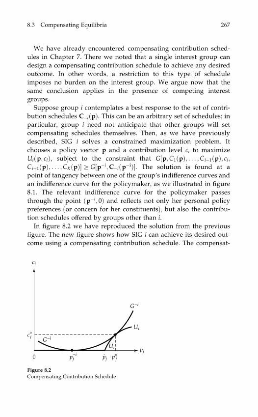
We have already encountered compensating contribution sched-

ules in Chapter 7. There we noted that a single interest group can

design a compensating contribution schedule to achieve any desired

outcome. In other words, a restriction to this type of schedule

imposes no burden on the interest group. We argue now that the

same conclusion applies in the presence of competing interest

groups.

Suppose group i contemplates a best response to the set of contri-

bution schedules C�iðpÞ. This can be an arbitrary set of schedules; in

particular, group i need not anticipate that other groups will set

compensating schedules themselves. Then, as we have previously

described, SIG i solves a constrained maximization problem. It

chooses a policy vector p and a contribution level ci to maximize

Uiðp; ciÞ, subject to the constraint that G½p;C1ðpÞ; . . . ;Ci�1ðpÞ; ci;Ciþ1ðpÞ; . . . ;CKðpÞ�bG½p�i;C�iðp�iÞ�. The solution is found at a

point of tangency between one of the group’s indifference curves and

an indifference curve for the policymaker, as we illustrated in figure

8.1. The relevant indifference curve for the policymaker passes

through the point ðp�i; 0Þ and reflects not only her personal policy

preferences (or concern for her constituents), but also the contribu-

tion schedules offered by groups other than i.

In figure 8.2 we have reproduced the solution from the previous

figure. The new figure shows how SIG i can achieve its desired out-

come using a compensating contribution schedule. The compensat-

Figure 8.2

Compensating Contribution Schedule


ing schedule, depicted by the heavy solid line, coincides with the

horizontal axis for policies pj a ppj and with the indifference curve

UiUi for policies pj > ppj. It has the same shape as the indifference

curve whenever contributions are positive. Faced with this schedule,

it is a best response for the policymaker to choose p�j . Evidently, the

SIG can always design such a compensating contribution schedule to

achieve its political objectives at no extra cost to itself.18

The fact that it is not costly for the interest groups to use compen-

sating schedules is perhaps not reason enough to focus on cases in

which they do. But the equilibria that arise when all contribution

schedules are compensating have two appealing properties. First,

these equilibria are always jointly efficient for the policymaker and

the interest groups. That is, when all of the SIGs offer compensating

schedules, the outcome is such that neither the policymaker nor any

SIG could be made better off by a different policy choice and set of

contribution levels without another SIG or the policymaker being

harmed. Efficiency is not a property shared by all equilibria of

common agency games. By using compensating schedules, the SIGs

eliminate the possibility that there will be unexploited gains in their

joint relationship with the policymaker.

Why is it that an equilibrium supported by compensating sched-

ules from all interest groups must be efficient? Intuitively, when

the contribution schedules are compensating, the SIGs confront the

policymaker with offers that accurately reflect their own evaluations

of the alternative policy options. Collectively, the offers give the

policymaker the appropriate incentive to weigh the conflicting

interests of the different interest groups.

More formally, we can prove that every compensating equilibrium

must be jointly efficient as follows. Suppose that some such equilib-

rium is not efficient. Then an alternative policy vector and list of

contributions exists, different from the equilibrium policy p� and

contributions c�, with the property that every interest group and the

politician are at least as well off under the alternative as in the equi-

librium, and at least one SIG or the politician is better off. Call the

alternative policy vector pp and the alternative vector of contributions

cc. Since, by hypothesis, group i is not worse off with policy pp and

18. A formal proof of this claim is provided by Bernheim and Whinston (1986a) for thecase of quasi-linear preferences, and extended by Dixit, Grossman, and Helpman(1997) to more general preferences.


payment cci than it is with policy p� and contribution c�i , it must be

that cci aHiðpp;U�i Þ, where Hiðp;U�

i Þ is the contribution schedule

employed by SIG i in the compensating equilibrium and U�i is its

resulting welfare level.

The fact that the policymaker chooses p� over the alternative pp in

the compensating equilibrium implies that Gðp�; c�ÞbG½pp;Hðpp;U�Þ�,where U� is the vector of equilibrium utility levels and Hð�Þ is the

vector of compensating contribution schedules. Since cci aHiðpp;U�i Þ

for every SIG i, it follows that G½pp;Hðpp;U�Þ�bGðpp; ccÞ. Finally, we

know that Gðpp; ccÞbGðp�; c�Þ, because the policymaker is by as-

sumption not worse off with policies pp and contributions cc than with

policies p� and contributions c�. These inequalities can be satisfied

only if Gðp�; c�Þ ¼ G½pp;Hðpp;U�Þ� ¼ Gðpp; ccÞ. But, if the policymaker

is indifferent between ðp�; c�Þ and ðpp; ccÞ, then there must be some SIG

i that strictly prefers ðpp; cciÞ to ðp�; c�i Þ. But SIG i could have induced

the policy choice pp with the contribution cci and an appropriately

designed contribution schedule.19 So it cannot prefer ðpp; cciÞ to

ðp�; c�i Þ. This is a contradiction. We conclude that if p� and c� are

outcomes in a compensating equilibrium, there are no alternative

policies and contributions pp and cc that make group i better off and no

group worse off.

The second reason why compensating equilibria may deserve spe-

cial attention is that these equilibria, and only these equilibria, are

what Bernheim and Whinston (1984) have termed ‘‘coalition proof.’’20

Bernheim and Whinston proposed the notion of a coalition-proof

Nash equilibrium as a refinement of the set of Nash equilibria. The

idea is that, if the players have an opportunity to engage in private

19. To see this final point, note that the policymaker is no worse off with policy p� andthe vector of contributions c� than she is with any other policy p 0 and contributionsH�iðp 0;U�Þ from the groups other than i and zero from group i; otherwise she wouldnot have chosen p� in the compensating equilibrium. But the policymaker is indiffer-ent between ðpp; ccÞ and ðp�; c�Þ, and ðpp; ccÞ is no worse for her than to choose pp and receiveH�iðpp;U�Þ from groups other than i and cci from group i, because the contributionsindicated by H�iðpp;U�Þ are no smaller than the corresponding elements of cc. It followsthat the policymaker also does not prefer any p 0 and contributions of H�iðp 0;U�Þ fromthe groups other than i and zero from i to pp and the contributions H�iðpp;U�Þ from thegroups other than i and cci from i. By appropriately designing the rest of its contribu-tion schedule, SIG i could have induced pp while paying cci.20. Peleg (1984) independently developed a similar concept, which he called a ‘‘quasi-coalitional equilibrium.’’ The proof that compensating equilibria are coalition proofand that any coalition-proof equilibrium of a common agency game can be imple-mented with compensating strategies can be found in Bernheim and Whinston (1986a).


and costless communication before the play of a game, then a subset

of them (the ‘‘coalition’’) might suggest to one another what strat-

egies they ought to pursue. These suggestions carry no commitment,

so they will be viable (if at all) only when it is indeed in the interest

of each member of the coalition to carry out its assigned action when

other members of the coalition do likewise. Bernheim and Whinston

have argued that, if every member of a coalition can better its lot

relative to some equilibrium by carrying out one such suggestion,

then the original equilibrium should not be considered stable.

Compensating equilibria are easier to characterize than other equi-

libria of political contribution games. These equilibria involve the

choice of only one item by each interest group. Each group might

choose, for example, a positive contribution for some particular

policy option. Then all other contribution levels are fixed by the joint

requirement that gifts cannot be negative and that, if positive, they

compensate for the difference in welfare under alternative options.

Moreover, it is often possible to use the efficiency property of com-

pensating equilibria to characterize what outcomes can occur.

In the remainder of this chapter we will examine the properties of

compensating equilibria in two examples. The first example focuses

on trade policy, the second on redistributive taxation. Together they

demonstrate how compensating equilibrium can be calculated in

particular applications while also providing insights into the prop-

erties of compensating equilibria that hold more generally.

8.4 Trade Policy

In this section we derive compensating equilibria of a game in which

interest groups representing different factors of production compete

for influence over a small country’s trade policy.

Consider the familiar Heckscher-Ohlin model of international

trade with two goods and two factors of production. Let the two

goods be footwear and consumer electronics, and the factors be

capital and labor. Each good is produced with constant returns to

scale and sold on a competitive world market. The small home

country faces a fixed world price of footwear equal to p�F and a fixed

world price of consumer electronics equal to 1.

The home country has an abundance of capital. Therefore, it

would import footwear (the labor-intensive good) in a free trade

equilibrium. A SIG representing the interests of labor covets a tariff


on imported footwear. Such a tariff would raise the relative domestic

price of footwear and consequently the real wage paid to labor, the

latter because labor is the factor used intensively in producing foot-

wear.21 A SIG representing the interests of capital would like a sub-

sidy to exports of consumer electronics. This policy is one that would

boost the real incomes of the capitalists. For the time being, we

ignore the world trade rules that prevent countries from subsidizing

their exports.

All individuals own either capital or labor, but not both. To make

matters simple, we adopt a particular form for an individual’s utility

function. We assume that each person has a function of the form

uðyE; yFÞ ¼ yE þ uFðyFÞ, where yE is his consumption of electronics

and yF is his consumption of footwear. With this utility function, an

individual buys footwear up to the point where the marginal utility

of shoe purchases, u 0FðyFÞ, equals the domestic relative price of foot-

wear, pF, and spends all remaining income on consumer electronics.

An individual who spends I achieves a utility level of I þ SðpFÞ, where

SðpFÞ is the consumer surplus derived from footwear purchases.22

A worker has two sources of income. He earns a wage w that

depends in equilibrium on the domestic price of footwear, pF. He

also receives a share of any tariff revenues. Tariff revenues are

tp�FmFðpFÞ, where t is the ad valorem tariff rate and mFðpFÞ is the

volume of imports, and each individual is assumed to receive the

same rebate. A typical worker also bears a per capita share of the cost

of any export subsidy. The subsidy costs are seEðpFÞ, where s is the

subsidy rate and eEðpFÞ denotes exports. Finally, the worker pays his

share of any contributions made by his interest group. We can write

the net income of a typical worker as

IL ¼ wðpFÞ þtp�

FmFðpFÞ � seEðpFÞNL þNK

� cLNL

;

where NL is the number of workers, NK is the number of capitalists,

and cL is the contribution by the labor SIG to the policymaker. The

goal of the labor SIG is to maximize UL ¼ NL½IL þ SðpFÞ�.Similarly, a capitalist earns income from her capital endowment

and she receives a share of any tariff proceeds. She helps to pay for

21. This is an implication of the well-known Stolper-Samuelson theorem: An increasein the price of a good increases the real income of the factor used intensively in pro-ducing that good, and decreases the real income of the factor used intensively in theother sector (see Stolper and Samuelson (1941)).22. Formally, SðpFÞ ¼ uFðy�

F Þ � pF y�F , when y�

F satisfies u 0Fðy�

F Þ ¼ pF.


the export subsidy and for any contributions that her interest group

makes. An individual who owns the average amount of capital, k,

has a net income of

IK ¼ rðpFÞk þtp�FmFðpFÞ � seEðpFÞ

NL þNK� cKNK

;

where rðpFÞ is the return on a unit of capital. The joint welfare of all

capitalists is UK ¼ NK½IK þ SðpFÞ�.The policymaker chooses the tariff rate t and the export subsidy

rate s to maximize a weighted sum of aggregate welfare and campaign

contributions. Aggregate welfare is NLIL þNKIK þ ðNL þNKÞSðpFÞ,while total contributions are cL þ cK. The policymaker’s objective is

G ¼ l½NLIL þNKIK þ ðNL þNKÞSðpFÞ� þ ð1� lÞðcL þ cKÞ;

with l < 12.23

We denote the (compensating) contribution schedules by HLðt; sÞand HKðt; sÞ. The two trade policies, together with the fixed interna-

tional prices, determine the domestic relative price of footwear,

pF ¼ð1þ tÞp�

F

1þ s; ð8:14Þ

which in turn determines the allocation of resources and the income

levels.

Finding a Nash equilibrium in contribution schedules might seem

a difficult task. However, we can use what we know about compen-

sating equilibria to characterize these outcomes. First, we know that

a compensating equilibrium must be jointly efficient for labor, capital,

and the politician. Joint efficiency means that G is maximized subject

to constraints on the levels of UL and UK. It is easy to see that this

requires a policy that maximizes the sum of private sector income

plus aggregate consumer surplus.24 But private sector income plus

23. For values of l > 1=2, the policymaker values the welfare of citizens higher thancampaign contributions, and so never accepts any contributions from the interestgroups.24. Let Y ¼ NLwðpFÞ þNKkrðpFÞ þ t p�

FmFðpFÞ � seEðpFÞ be private-sector income. Then

G ¼ l½Yþ ðNL þNKÞSðpFÞ� þ ð1� 2lÞðcN þ cKÞ:

If the labor and capital SIGs must achieve utility levels of UL and UK, respectively,then

cN þ cK ¼ Yþ ðNL þNKÞSðpFÞ �UL �UK;

in which case maximizing G is the same as maximizing Yþ ðNL þNKÞSðpFÞ.


aggregate consumer surplus are maximized when pF ¼ p�F , that is,

when the domestic relative price of footwear is equal to the world

relative price. Therefore, s� ¼ t� in any compensating equilibrium

(see (8.14)).

Whenever s ¼ t, all resource allocations and (gross) income levels

are the same as in free trade. Thus, the competition for influence

results in a stalemate. The labor SIG wants a high tariff and a low

export subsidy, whereas the business group wants a low tariff and a

high subsidy. Since neither policy increases the total economic pie

and there are no other groups in the economy to exploit, the equi-

librium outcome favors neither group. What is worse for the groups

is that they do not achieve this standoff costlessly. In fact, each group

must contribute positively to secure the equivalent of a free trade

outcome. If a group were to withhold its contributions, it would

suffer yet a worse fate than it does with the neutral policies.

We derive the equilibrium contributions in two steps. First, we

make use of the fact that a compensating schedule calls for a pay-

ment, if positive, that compensates for any differences in utility rela-

tive to the equilibrium utility level. In the equilibrium, the aggregate

utility of labor equals U�L ¼ NL½wðp�

FÞ þ Sðp�FÞ� � c�L. The contribution

schedule of the labor SIG thus can be written as

HLðs; tÞ

¼ max NL½wðpFÞþSðpFÞ� þNL

NLþNK½tp�

FmFðpFÞ�seEðpFÞ��U�L; 0

� �;

where pF ¼ ð1þ tÞp�F=ð1þ sÞ. The contribution schedule of the capital

SIG is analogous.

Now that we have the form of the contribution schedule, we can

find the policy that the politician would choose in the absence of con-

tributions from the capital SIG. In such circumstances, the policy-

maker would maximize

G�K ¼ l½NLIL þNKIK þ ðNL þNKÞSðpFÞ� þ ð1� lÞHLðs; tÞ;

a weighted sum of aggregate welfare and contributions from the

labor group. This maximization results in policies that imply a rela-

tive price p�KF > p�

F . Without contributions from capital, trade policy

would favor the labor SIG, which means that the domestic relative

price of footwear would be greater than the world price. This would

give the workers a real income higher than under free trade. The


policymaker can induce a domestic price of p�KF by enacting either a

tariff (t > 0), an export tax (s < 0), or a combination of the two; see

equation (8.14).

Similarly, we can calculate the policies that the politician would

set in the absence of contributions from the labor group. These poli-

cies are the ones that maximize

G�L ¼ l½NLIL þNKIK þ ðNL þNKÞSðpFÞ� þ ð1� lÞHKðs; tÞ:

In this case, the policymaker would choose policies that result in the

domestic relative price p�LF < p�

F . She could do so by enacting a sub-

sidy to exports, a subsidy to imports, or a combination of the two.

Such policies would reduce the relative price of footwear, and so

boost the real income of capital.

It is these policies, leading to p�KF and p�L

F , that the interest groups

must guard against. The labor SIG must give a sufficient contribution

to ensure that the policymaker chooses the equilibrium policies and

not ones that result in a domestic relative price of pF ¼ p�LF . This re-

quirement pins down the size of c�L. Similarly, the capital SIG must

contribute sufficiently so that the policymaker chooses the equilib-

rium policies and not ones that lead to pF ¼ p�LF . This determines c�K.

In the equilibrium, the policymaker achieves an efficient allocation

of resources and collects political tributes from both interest groups.

This outcome is typical of situations in which the policymaker cares

about aggregate welfare and all members of society are represented

by some interest group or another.25

Let us briefly consider how our conclusions would change if we

introduce a prohibition on export subsidies. Such a prohibition was

incorporated into the original articles of the General Agreement on

Tariffs and Trade (GATT) and remains a part of the trading rules

today. As the formula for domestic prices reveals, the effects of an

export subsidy (with s > 0) can be mimicked by the use of a subsidy

to imports (t < 0).26 If a prohibition on export subsidies is to have

any real effects, it must be coupled with a rule preventing import

subsidies as well. So, suppose that the political competition plays out

25. Note that, in the compensating equilibrium, factor incomes are the same as in freetrade, there is no net government revenue to redistribute, and the citizens all share inthe cost of political contributions. Thus the competition for influence leaves everyone(except the politician) worse off than in a world without influence payments.26. The equivalence between export subsidies and import subsidies is known in theinternational trade literature as the Lerner symmetry theorem.


subject to the constraints that sa 0 and tb 0. These constraints do

not alter the conclusion that the policy outcomes must be jointly

efficient for the interest groups and the policymaker. Recall that

unconstrained joint efficiency required pF ¼ p�F , or s ¼ t. The same

outcome can be achieved subject to the policy constraints, but only

if s ¼ t ¼ 0. Thus, we now have an unambiguous prediction about

the trade policies, but of course the same resource allocation as we

had without the constraints. The contributions that support the

equilibrium are not, however, the same as before. In particular, in

the absence of contributions from labor, the government could not

choose policies that reduce the domestic relative price of footwear.

Such domestic prices require an export subsidy or an import subsidy,

both of which are not feasible. Accordingly, p�LF ¼ p�

F under the new

rules of the game; that is, the policy choices are the same whether the

labor SIG contributes to the policymaker or not. In equilibrium, the

labor SIG has nothing to fear from its rival interest group, and so it

refrains from contributing.

To summarize, a rule prohibiting export subsidies and import

subsidies has no effect on the equilibrium allocation of resources and

(essentially) no effect on the policy choice. Such a rule does, however,

have distributional implications for the policymaker and the interest

groups. Since the threat of export subsidies no longer exists, the

position of the policymaker has been weakened vis-a-vis the labor

group. The labor SIG achieves higher utility, and the politician lower

welfare, when export subsidies are prohibited than when they are

allowed.

8.5 Redistributive Taxation

In this section we study the political economy of income redistribu-

tion. We assume that the policymaker’s objective function includes

as arguments the utility levels of all members of society and the total

amount of her campaign contributions. This objective function could

reflect her personal aversion to inequality—she might prefer, for

example, a situation in which all individuals have roughly the same

level of utility to one in which some individuals are very well off and

others are not—or it might be that individuals base their voting

decisions on their personal levels of well-being and the politician is

concerned about her chances of being reelected. In the latter case, the

politician’s objective function might give greater weight to certain


individuals, if for example some of them are more likely to turn out

to vote than others or if their voting behavior is more responsive

to their level of personal well-being. We write G ¼ GGðU; cÞ, where

U ¼ ðU1; . . . ;UNÞ is the vector of utility levels of the N members of

society and c ¼P

ci. Here, an individual may belong to one interest

group, several, or none. The individual i has a utility function

Uiðp; ciÞ, where p is a vector of policy outcomes and ci is the total

amount of her payments to the various SIGs of which she is a

member, which in turn contribute to the policymaker.

Interest groups are arbitrary collections of individuals. SIG 1 might

have individuals 1, 7, 12, 16, and others as members, while SIG 2 has

individuals 2, 7, 13, 15, and so on as members. Notice that in this

example, individual 7 is a member of both groups. All that we insist

on is that each SIG maximize an objective function that includes the

utility levels of all of its members as arguments. The groups offer

compensating contribution schedules to the policymaker and allo-

cate the burden of their contributions to their members in whatever

manner they choose.

This formulation has one distinguishing feature. Economic policies

affect the welfare of the citizenry, which in turn affects the policy-

maker’s welfare. But the policymaker has no personal preferences

about policy outcomes beyond their impact on her constituents.

In other words, the vector p enters GGð�Þ only indirectly through

U1ðp; c1Þ, U2ðp; c2Þ, and so on; it does not appear as a separate argu-

ment in this function.27 For now, we take p to be an arbitrary set of

feasible policies. It might include, for example, subsidies to produc-

tion, regulations on the use of certain factors, taxes or subsidies on

trade, and other policies. We assume that GGð�Þ is strictly increasing in

all of its arguments.

We are now ready to describe an important property of compen-

sating equilibria in this rather general setting. It can be shown that all

compensating equilibria are constrained Pareto efficient. That is, in

any compensating equilibrium, there exists no alternative vector of

policies among those that are feasible and no alternative vector of

contributions yielding the same total contribution with the property

that all individuals (including those who are members of SIGs and

those who are not) are at least as well off under the alternative poli-

27. Similarly, the policymaker cares about the sources of her contributions only inso-far as the distribution of payments affects the utility levels of her various constituents.


cies and contributions as in the compensating equilibrium, and at

least one individual is better off.28

This property of a compensating equilibrium is stronger than the

one we identified earlier. Here the outcome must be efficient not

only for the policymaker and the organized special interests, but also

for the polity as a whole. The key to the strengthening of our earlier

result is the assumption that GGð�Þ is increasing in each Ui. Pareto effi-

ciency is achieved now, because the policymaker values an increase

in the welfare of each and every citizen. Were the equilibrium not

efficient, it would be possible to raise the policymaker’s objective

function without harming any of the interest groups. But this would

violate the joint efficiency property of a compensating equilibrium.

Armed with this result, we can make many predictions about

economic policy. In fact, we can draw on the large literature on

economic policy that takes a normative approach. The normative

literature is meant to be prescriptive, not predictive of the outcome

of any political process. But now we can apply its findings to char-

acterize equilibria of a well-specified game of political influence.

Take, for example, a pure case of redistributive taxation. Suppose

that an individual’s utility depends on his own consumption of a

vector of goods and on his labor supply. Let goods be produced by

profit-maximizing firms that operate under constant or decreasing

returns to scale. Let there be perfect competition in all goods and

factor markets, and no externalities or other rigidities in the economy.

The economy is either closed to international trade or small in world

markets. In this setting, if lump-sum taxes and transfers are feasible,

Pareto efficiency is achieved by an appropriate set of such taxes and

transfers and without any other government intervention of any

sort.29 The absence of distortionary taxes, subsidies, and regulations

ensures economic efficiency. Only the lump-sum transfers and sub-

sidies are used in response to the groups’ political pressures, which

are reflected in their compensating contribution schedules. They give

rise to an equilibrium distribution of income.

28. This property of compensating equilibria follows almost immediately from ourearlier result that all compensating equilibria are jointly efficient for the group of SIGsand the policymaker. A formal proof of the constrained efficiency result can be foundin Dixit, Grossman, and Helpman (1997).29. The closed-economy version of this result is a corollary of the second theorem ofwelfare economics; see Samuelson (1947). Dixit (1987) extended the result to a smallopen economy. In a large economy that engages in trade, the lump-sum taxes andtransfers must be supplemented by a set of ‘‘optimal’’ tariffs and export taxes.


Many economists have noted that lump-sum taxes and transfers

are difficult to implement. They require that the policymaker have

perfect information about individuals’ preference and abilities. In

practice, the policymaker is not born with such information but

needs to gather it by surveying the population or by observing its

behavior. But if the individuals know that their tax liabilities will

depend on their verbal responses or their economic behavior, they

will have incentive to distort their words and actions in order to

reduce their burden. Accordingly, lump-sum taxes and transfers may

not be feasible. In the event, we can apply the findings of Diamond

and Mirrlees (1971) to characterize the compensating equilibria. They

have shown that when the government of a closed economy is con-

strained not to use lump-sum taxes or transfers, a Pareto efficient

equilibrium requires the use of only taxes and subsidies on consump-

tion and factor supplies, with no taxes or subsidies to output by

particular industries, and no taxes or subsidies for the use of partic-

ular factors of production.30 Once again, the normative prescriptions

of an earlier literature become predictions about the equilibrium

outcome in an influence game.

Finally, let us say a few words about the contributions that support

a compensating equilibrium in a political game of income redistribu-

tion. Here we report the findings of Dixit, Grossman, and Helpman

(1997). They show, first, that if lump-sum taxes and transfers are

feasible as policy instruments, then the competition for influence will

be very intense. Specifically, if no individual belongs to every inter-

est group and if there are at least two such organized groups, then

a member of a SIG will fare no better in the equilibrium than she

would if her group were to unilaterally renounce its political activ-

ities. In other words, the policymaker captures all of the surplus in

her relationship with the various interest groups. The policymaker

achieves the same level of political welfare in the compensating

equilibrium as she would in a setting where she could dictate not

only the allocation of resources to various economic uses, but also

the levels of campaign contributions by every group!

When the policymaker has complete freedom to fashion lump-sum

taxes and transfers, she enjoys enormous political power. This power

30. Dixit (1987) provides the extension of this result to the open economy. He showsthat efficiency requires free trade in a small economy, but a set of optimal tariffs andexport taxes in an economy that is large enough to affect its international terms oftrade.


emanates from the ability she has to cease her dealings with any SIG

at no cost to herself. For, suppose that a deviant SIG were to demand

some positive surplus from the policymaker in exchange for its con-

tribution. The policymaker could reduce the transfer to this group

(or increase the tax) by the amount of its equilibrium contribution

and redirect the funds to the members of some other SIG. Since the

SIGs all have compensating payment schedules, the policymaker

would receive back from the recipients the entire amount of the

redirected transfers as additional contributions. So the policymaker

would not lose any contributions by this change, nor would the wel-

fare of any individual be altered. Thus, the policymaker is indifferent

between dealing with the deviant group or not. For this reason, the

group cannot succeed in its attempts to share in the surplus.

When lump-sum taxes and transfers are not feasible, the SIGs may

fare better in their relationship with the policymaker. Typically, none

of them is willing to renounce its political activity in such circum-

stances, because all enjoy some surplus in the political equilibrium.

In the absence of lump-sum tools for redistribution, if any SIG were

to withhold its promised contribution, the policymaker would be

forced to resort to distortionary taxes or subsidies if she wished to

make up for the potential loss of campaign funds with greater gifts

from other groups. But this would exacerbate economic inefficien-

cies, with resultant costs to society and the policymaker. Since the

policymaker could not costlessly replace the gifts from a SIG with

gifts from the others, each group can extract surplus by the implicit

threat to withdraw from the deal. In fact, the less economically effi-

cient are the tools of redistributive politics, the better is the bargaining

position of the organized interest groups vis-a-vis the policymaker.

8.6 Competition for Influence: Good Thing or Bad Thing?

Our analysis sheds light on a controversy in the literature on interest-

group competition. Some authors, following Becker (1983), believe

that competition between interest groups is beneficial to society.

Using a reduced-form model in which the government responds to

‘‘pressures’’ from special interests, Becker showed that competition

can lead to Pareto efficient policies as the groups attempt to generate

the greatest benefit for themselves, given the cost imposed on others.

Tullock (1980) and others have argued differently. They see the rents

created by policy being dissipated by socially wasteful expenditures.

8.6 Competition for Influence: Good Thing or Bad Thing? 279

In a simple model with risk-neutral groups in which each SIG has a

probability of capturing a given rent that is proportional to the size

of its investment in ‘‘rent-seeking activities,’’ the fraction of the rent

that is dissipated increases with the number of competitors. In this

sense, competition among groups is harmful to society. Our more

complete model of intergroup competition reveals that there is some

element of truth in both of these positions.

In Dixit, Grossman, and Helpman (1997), the authors identify cir-

cumstances under which the equilibrium policies are bound to be

efficient. If the SIGs all use compensating contribution schedules, the

policymaker has no direct preferences over the policies except inso-

far as they affect her constituents’ welfare, and if the objective func-

tion of the policymaker increases, however slightly, with an increase

in the well-being of any constituent, then the competing bids for

influence must result in a choice that is Pareto efficient among the set

of feasible policies.31 This means that, given the initial set of contri-

bution levels—positive for members of some interests groups and

zero for those who are not in any SIG—there is no feasible, alterna-

tive policy vector that could make some individual better off without

making someone else worse off.

This, however, does not mean that competition between interest

groups serves the SIG members well. As we have seen, the equilib-

rium outcome is supported by a set of political contributions. Some

may regard the campaign spending funded by SIG contributions as a

waste of resources. In any case, the contributions represent a dissi-

pation of rents from the groups’ perspective, as predicted by Tullock

and others. When a fixed quantity of rents is up for grabs, it takes a

large number of competitors to generate full dissipation. But when,

as here, the quantity of rents is determined in the political equilib-

rium, the outcome can be even more dire. As mentioned previously,

Dixit et al. consider a situation in which income can be transferred

between groups without the creation of any deadweight loss. In such

circumstances, competition between two interest groups is enough to

dissipate fully the benefits from political activity. That is, each SIG

fares no better in the political equilibrium than it would if it were to

renounce entirely its efforts to curry favor.

31. Alternatively, efficiency will result even if the policymaker does not care about thewelfare of her constituents, if each citizen belongs to an interest group and none is amember of more than one group.


The highly adverse effects of competition do, however, require

some special conditions. Rents are fully dissipated only if utility can

be transferred costlessly between groups, so that the recipient’s gain

from a change in policy exactly matches the payor’s loss. If instead

there are institutional constraints or feasibility constraints that force

the policymaker to resort to redistributive instruments that generate

deadweight loss, the interest groups will be able to capture some of

the surplus in their political relationship with the policymaker.

Whether the addition of more groups to compete with an initial set

of SIGs will benefit or harm the typical group member, and whether

it will benefit or harm those who are not represented by any SIG,

depends on how the various interests align on the issues and on the

nature of the policy decisions that are subject to influence.

In this chapter, we have studied the competition among SIGs for

political influence. We modeled this competition as one in which

each of several (or many) SIGs confronts the policymaker with offers

of campaign contributions in exchange for various policies. An equi-

librium is a set of contribution schedules that are mutual best re-

sponses, considering the anticipated behavior by the policymaker.

Typically there are many equilibria of such influence games. But

the set of possible outcomes is narrowed considerably when we

place reasonable restrictions on the form of the equilibrium contri-

bution schedules. Using an assumption that the schedules are differ-

entiable when positive, we are able to characterize the set of possible

policy outcomes. With a further assumption that the schedules are

compensating, we are also able to characterize the equilibrium con-

tributions. We illustrated the general theory in several applications.

Throughout this chapter and the last, we have assumed that a

unitary policymaker has unilateral authority to enact policies. Inter-

preted literally, this assumption renders the policymaker an omnip-

otent executive. But our analysis may also apply to settings with

legislative decision making, provided that a single political party

controls a majority of votes and that the delegates succumb to strict

party discipline. When a legislature comprises members who vote

independently and pursue their own objectives, the problem of

buying influence is likely to be more complex. We turn to this prob-

lem in the next chapter.

8.6 Competition for Influence: Good Thing or Bad Thing? 281

9 Influencing a Legislature

In the last two chapters we assumed that policies are set by a single

individual or by a cohesive, well-disciplined political party. In real-

ity, of course, most policy decisions are made not by one person but

by a group of elected representatives acting as a legislative body.

Even when the legislature is controlled by a single party, the dele-

gation members do not always follow the instructions of their party

leaders. In situations with multiple, independent legislators, interest

groups face a subtle problem in deciding how best to use their

resources to influence policy choices. A SIG must decide where to

concentrate its bid for influence and what actions it should try to

affect. Should the group seek to solidify support among those legis-

lators who would be inclined to support its positions anyway, or

should it seek to win over those who might otherwise be hostile to its

views? Should it focus mostly on buying votes for bills that it likes,

or on influencing the legislators who might be deciding the bills’

contents? Is it necessary to influence those who are drafting the bills

initially, or is it enough to curry favor among those who will be in a

position to offer amendments? The answers to these questions and

others like them surely depend on the rules of the legislative process

—for example, on how the agenda is determined and on what pro-

cedures are used for introducing and dispensing with amendments.

In other words, the optimal strategy for wielding influence will vary

with the institutional setting.

Beginning with Gilligan and Krehbiel (1987, 1989) and Baron

and Ferejohn (1989), social scientists have developed formal models

of the legislative process. These models emphasize how policy out-

comes may vary with differences in procedures and differences in the

structure of the political system. Procedural variation might include,

for example, a comparison of ‘‘open rules,’’ which allow members of

the legislature to offer amendments to bills proposed to the body,

and ‘‘closed rules,’’ which prohibit such amendments. Structural

variation might entail a comparison of congressional systems, in

which members represent geographic regions and have relatively

weak party loyalty, and parliamentary systems, where parties com-

pete nationally and party loyalty is strong.1 In most of this research,

attention has been focused on the interaction between a group of

legislators who have conflicting preferences. The question has rarely

been raised of how these preferences relate to those of voters, on the

one hand, and to the actions of SIGs on the other.2

This chapter aims to include both influence activities and legis-

lative procedures in a single model, to see how the two interact in

determining policy. Our approach will be to think of contribution

offers as inducing preferences for the legislators, who then must

interact in the parliament according to the rules of the legislative

game. By taking this approach, we hope to shed light on what strat-

egies interest groups might pursue to exert their influence over a

legislature, and how the conflicts between interest groups might be

resolved. Since this analysis is considerably more complex than what

we have seen until now, we will present only a brief introduction to

some of the issues that can arise. We begin with the case of a single

interest group and then proceed to the case of competing interests.

9.1 Buying Votes

Consider a situation in which a legislature will decide a policy issue.

An organized interest group seeks to influence the decision. The

group’s preferences are represented by Uðp; cÞ ¼ WðpÞ � c, where c

now denotes the total of its campaign contributions. The group can

contribute to one or more of the members of the legislature.

The legislature has three members. We choose the number three

because it is the smallest number that allows for both legislative

1. Persson, Roland, and Tabellini (2000) have examined the budgetary process underthese alternative systems. See also Baron (1991, 1993) and Diermeier and Feddersen(1998).2. Austen-Smith and Banks (1988) and Chari, Jones, and Marimon (1997) are excep-tions. These authors have incorporated both electoral competition and legislative bar-gaining in a single model.


deliberations and majority rule. We will refer to the legislators as

L1, L2, and L3. Legislator Li seeks to maximize GLiðp; ciÞ ¼ lWLiðpÞ þð1� lÞci, which is a weighted average of his subjective evaluation of

the policy outcome and his campaign receipts. Preferences like these

may arise, for example, if legislator Li represents a district whose

aggregate welfare is WLið�Þ and he cares about the well-being of his

constituents as well as his campaign finances. In Chapter 10 we will

see how an objective function like this can be derived from purely

political objectives, such as a candidate’s desire to win an election or

a party’s wish to maximize its patronage.

In this section we follow Snyder (1991) in assuming that the SIG

has the ability to set the political agenda. That is, the SIG can pro-

pose a bill and offer contributions to some or all of the legislators in

order to encourage their support.3 The sole job of the legislature is to

ratify or reject the group’s proposal. This modeling of the legislative

process is, of course, unrealistic. But it does provide for a simple

analysis with several useful insights. In the next section we will des-

ignate one of the legislators to be the agenda setter; in such a setting

both the policy outcome and the structure of contributions may be

somewhat different from what we observe here.

The contribution-cum-legislative game plays out as follows. First,

the interest group proposes a policy level p and makes a separate

contribution offer to each legislator. It promises to contribute ci to

legislator Li if the legislator votes in favor of the bill. The voting

pits the proposed legislation against a status quo policy, which we

denote by q. If at least two of the legislators vote for the bill, then p

is implemented as policy. Otherwise, the outcome is q. Finally, the

SIG contributes to the various campaigns in accordance with its

promises.4

We begin the analysis with the second stage, which arises after

the bill has been drafted and the SIG has tendered its offers to the

members of the legislature. Consider a legislator who expects not to

3. Snyder (1991), who developed a model with many legislators, also studied the casein which the SIG must offer the same payment to any supporter of its proposed legis-lation. This constraint on SIG contributions seems artificial to us, so we will not con-sider it here.4. In principle, the SIG might also offer a contribution ci to legislator Li if Li votesagainst the proposal. However, it is fairly obvious that the SIG has no reason to paythe legislator to oppose its own proposal. We avoid the unnecessary notation andsimply observe that contributions to nonsupporters are optimally set to zero.


be pivotal: he expects the bill surely to pass or surely to fail no matter

how he votes. Such a legislator will vote in favor of the proposal if he

is offered any positive inducement to do so, and he will be indifferent

about his vote if no contribution is offered. We assume that the leg-

islator responds to such indifference by voting for whichever policy

option he prefers.

Now consider a legislator Li who anticipates that his vote will be

decisive. If Li votes in favor of the bill, it passes, and he attains utility

lWLiðpÞ þ ð1� lÞci. If he votes against the bill, it fails, and the legis-

lator’s utility is lWLiðqÞ. Clearly, Li will vote for the bill when he

expects to be pivotal if and only if lWLiðpÞ þ ð1� lÞci b lWLiðqÞ.5We turn next to the problem facing the interest group. Anticipat-

ing the behavior of the legislators, the SIG must decide what bill to

propose and what contributions to offer. For simplicity, suppose that

WðpÞ and all WLiðpÞ are single-peaked functions and that the policy

must be chosen from a range of feasible policies. Under these con-

ditions, each legislator has a unique favorite policy among those that

are feasible, and so does the SIG. Denote by p the ideal policy for the

SIG and by pLi the ideal policy for legislator Li.

If at least two of the legislators prefer p to q, the solution to the

SIG’s problem is simple. In such circumstances, the group should

propose its favorite policy and offer nothing to the legislators. The

two (or three) legislators who prefer p to q will vote in favor of the

bill, which thus becomes law. In the resulting equilibrium, the SIG

attains its optimal combination of p ¼ p and c ¼ 0.

When at least two of the legislators prefer q to p, the situation

is different. Then the group must either compromise on its policy

demands or offer contributions in exchange for support. We proceed

now to consider which legislators are targeted, how much they

receive, and what policy is proposed.

Clearly, the SIG would like to buy support for any bill p at the

minimum total cost. If a legislator Li prefers p to q, then his vote

comes for free. Otherwise a payment must be made, the size of which

depends on whether Li expects to be pivotal or not. One possibility is

that none of the legislators who prefer q to p expects to be pivotal in

5. Technically, the legislator is indifferent between the options when lWLiðpÞ þð1� lÞci ¼ lWLiðqÞ. Since the SIG could always resolve this indifference by offering abit more for the legislator’s support, a legislator who expects to be pivotal breaks anyties in favor of the proposal.


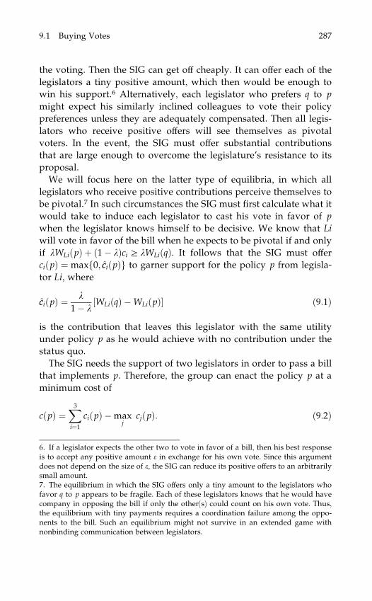
the voting. Then the SIG can get off cheaply. It can offer each of the

legislators a tiny positive amount, which then would be enough to

win his support.6 Alternatively, each legislator who prefers q to p

might expect his similarly inclined colleagues to vote their policy

preferences unless they are adequately compensated. Then all legis-

lators who receive positive offers will see themselves as pivotal

voters. In the event, the SIG must offer substantial contributions

that are large enough to overcome the legislature’s resistance to its

proposal.

We will focus here on the latter type of equilibria, in which all

legislators who receive positive contributions perceive themselves to

be pivotal.7 In such circumstances the SIG must first calculate what it

would take to induce each legislator to cast his vote in favor of p

when the legislator knows himself to be decisive. We know that Li

will vote in favor of the bill when he expects to be pivotal if and only

if lWLiðpÞ þ ð1� lÞci b lWLiðqÞ. It follows that the SIG must offer

ciðpÞ ¼ maxf0; cciðpÞg to garner support for the policy p from legisla-

tor Li, where

cciðpÞ ¼l

1� l½WLiðqÞ �WLiðpÞ� ð9:1Þ

is the contribution that leaves this legislator with the same utility

under policy p as he would achieve with no contribution under the

status quo.

The SIG needs the support of two legislators in order to pass a bill

that implements p. Therefore, the group can enact the policy p at a

minimum cost of

cðpÞ ¼X3i¼1

ciðpÞ �maxj

cjðpÞ: ð9:2Þ

6. If a legislator expects the other two to vote in favor of a bill, then his best responseis to accept any positive amount e in exchange for his own vote. Since this argumentdoes not depend on the size of e, the SIG can reduce its positive offers to an arbitrarilysmall amount.7. The equilibrium in which the SIG offers only a tiny amount to the legislators whofavor q to p appears to be fragile. Each of these legislators knows that he would havecompany in opposing the bill if only the other(s) could count on his own vote. Thus,the equilibrium with tiny payments requires a coordination failure among the oppo-nents to the bill. Such an equilibrium might not survive in an extended game withnonbinding communication between legislators.


As suggested by Riker’s ‘‘size principle,’’ the SIG achieves the lowest

cost by forming a ‘‘minimum winning coalition’’ among those mem-

bers of the legislature who are most sympathetic to p relative to the

status quo.8

We can now use the function cðpÞ to solve the broader problem

facing the interest group. The SIG seeks the feasible policy that

maximizes its utility net of contributions. Formally, the equilibrium

policy p� solves

p� ¼ arg max U½p; cðpÞ� ð9:3Þ

for p between pmin and pmax. In equilibrium, the SIG pays c�i ¼ ciðp�Þto the legislators who are induced to support the bill.

Figure 9.1 depicts the functions cciðpÞ for a case in which q < pL1 <

pL2 < pL3. In the figure, a legislator’s favorite policy pLi can be found

at the value of p for which cciðpÞ attains a minimum. In drawing the

figure, we have also assumed that cc1ðpÞ < cc2ðpÞ < cc3ðpÞ for all p < q,

while cc1ðpÞ > cc2ðpÞ > cc3ðpÞ for all p > q. In other words, not only is

the favorite policy of L3 greater than that of L2, which in turn is

greater than that of L1, but L3 has the relatively strongest pref-

erence for all policies p greater than the status quo, and L1 has the

8. See Riker (1962) for the original statement. Riker and Ordeshook (1973, Chapter 7)provide a formal discussion and some empirical evidence.

Figure 9.1

Compensation Functions for Legislators


relatively strongest preference for all policies less than the status

quo.9

Using figure 9.1, we can construct the function cðpÞ. Consider firsta policy p < q. Since all legislators prefer the status quo to any such

policy, the SIG must buy two votes to effect such an outcome. To do

so, it is least costly for the group to procure the support of legislators

L1 and L2. These two have the least distaste for policies with a small

value of p, so the cost of influencing them is less than for L3. For all

policies p < q, then, cðpÞ ¼ cc1ðpÞ þ cc2ðpÞ.Next consider a policy p between q and p2. For all such values of p,

at least two (and sometimes three) of the legislators prefer the pro-

posal to the status quo. Thus, the SIG can effect any such policy at

zero cost.

For policies to the right of p2, the SIG must offer contributions to at

least one legislator. The vote of legislator L2 is available to the SIG at

a lower cost than that of L1. Accordingly, for policies between p2 and

p3, the SIG pays cc2ðpÞ to L2, and gains the support of L3 without cost.

Finally, for policies p > p3, the SIG must contribute to two legislators

in order to enact its proposal. It chooses L2 and L3 as the least costly

to influence, so that cðpÞ ¼ cc2ðpÞ þ cc3ðpÞ. We have thus completed the

construction of cðpÞ, which is shown as the bold curve in figure 9.2.

We can now identify the equilibrium policy for different preferences

of the interest group. The SIG achieves highest utility for any given c

when p ¼ p. Thus, its indifference curves are a set of inverted U-

shaped curves, each with a peak at p ¼ p. First consider a case where

the group’s ideal policy p is far to the left of q. Then the SIG achieves

its highest utility for some policy p� between p and q, as shown in

Panel a of figure 9.3, in which UU is the SIG’s indifference curve. Here

the SIG pays contributions to legislators L1 and L2, but it also com-

promises its policy goals. The policy outcome falls somewhere be-

tween the status quo and the group’s ideal policy. Panel b of figure 9.3

illustrates a different case, where the SIG’s favorite policy is only

slightly smaller than the status quo q. Here the group contents itself

with the status quo policy. Evidently, the benefit to the group from

achieving a policy smaller than q in this situation is not worth the cost.

Now consider the case in which the group’s ideal policy lies to

the right of the status quo. We have already noted that, when p lies

9. The situation depicted in the figure applies, for example, when the utility func-tions are quadratic; that is, WLiðpÞ¼ �ðp�pLiÞ2, in which case cciðpÞ¼ ½l=ð1� lÞ��ðp�qÞðpþq�2pLiÞ. Snyder analyzes this case of quadratic utility functions in his 1991paper.


Figure 9.2

The Cost of Legislation

Figure 9.3

Equilibrium Policy without an Agenda Setter


between q and p2, the SIG can attain its favorite outcome at zero cost.

The group simply proposes its ideal policy and watches as (at least)

two of the legislators vote in favor of the bill. When the SIG’s ideal

policy exceeds p2, this strategy will not work. Then the reasoning is

similar to the case of p < q. When p > p2 by only a small amount, the

group contents itself with the policy p ¼ p2, which it can achieve at

zero cost. As the group become more extreme in its preferences, it

eventually wishes to implement a policy greater than p2. To do so, it

contributes to the campaign of legislator L2 and possibly to that of

legislator L3 as well.

Notice who are the recipients of the group’s contributions in each

case. A legislator with preferences very different from the SIG does

not receive any contributions, because the group only needs a ma-

jority of votes, and these unsympathetic legislators are too costly to

win over. Only the most sympathetic legislators are included in the

minimum winning coalition. But a legislator with preferences very

similar to those of the group does not receive contributions either.

Such a legislator is ready to support the group’s bill without any

added inducement. Rather, it is the legislators whose preferences

differ from the group by an intermediate amount who capture the

largest donations.

We can use a similar approach to analyze a situation in which one

of the legislators has an ideal policy on the opposite side of the status

quo from the favorite policies of the other two; for example, pL1 <

q < pL2 < pL3. In such circumstances, the function cðpÞ has a flat por-

tion to the right of q, just as in figure 9.2. In other words, there again

is a range of proposals p > q that will receive the support of legisla-

tors L2 and L3 without any positive contributions. But now there is a

range of policies to the left of the status quo that the SIG can imple-

ment with contributions only to L2. In any case, the main conclusions

still apply. The SIG builds a minimum winning coalition among the

legislators whose preferences are most similar to its own, and con-

tributes the most to the legislator whose preferences are neither the

most similar nor the most different.

9.2 A Legislature with an Agenda Setter

The Snyder model, while analytically convenient, gives too much

power to the interest group. Not only can the SIG use its resources to

influence the legislators’ voting behavior, but it can also dictate the


provisions of the law that stands as an alternative to the status quo.

In reality, interest groups have no such authority to introduce bills to

the legislature. But they can use their resources to influence those

who do have this authority.

In order to understand how this might work, we need a more com-

plete description of the legislative process. A useful starting point is

the elegant model of legislative bargaining formulated by Baron and

Ferejohn (1989). In this model, an ‘‘agenda setter’’ occupies center

stage. The agenda setter—who might be the chair of the relevant

committee of the U.S. Congress, or the relevant minister in a parlia-

mentary system—has the sole authority to propose new legislation.

Once the agenda setter drafts a bill, it comes to the floor for delib-

eration and a vote. At this stage the parliamentary rules dictate

whether representatives can amend the proposal and, if so, by what

means. Then the legislators vote on the bill (amended or not) to

determine whether it will replace the status quo.

We introduce an interest group into the Baron-Ferejohn frame-

work. The SIG can seek to influence the agenda setter but cannot

usurp his authority. We imagine that the SIG can offer campaign

contributions both to the agenda setter and to other members of the

legislature. First the SIG meets with the agenda setter and confronts

him with a contribution schedule. This schedule associates a dona-

tion with each bill that the agenda setter might sponsor. The agenda

setter receives the specified contribution caðpÞ if he proposes a bill

that implements p and continues to support it when it comes to a

vote. After the agenda setter has drafted a bill, the SIG can meet

privately with the remaining legislators. At these meetings, the SIG

can offer a contribution in return for a vote in favor of the proposed

legislation, or it can offer one to encourage a vote against. To keep

matters simple, we assume a closed parliamentary rule that excludes

the possibility of amendments. Thus, after all of the offers are ten-

dered, the legislators vote on the bill as originally proposed.

It is easy to see that the equilibrium of this legislative game need

not be the same as in the Snyder model. For example, suppose the

legislators’ preferences give rise to compensation functions such as

those depicted in figure 9.1, and suppose that the SIG’s ideal point p

lies well to the left of the status quo. Recall the equilibrium (illus-

trated in Panel a of figure 9.3) that arises when the SIG dictates the

content of legislation. The group chooses a policy p� to the left of

q and makes contributions to L1 and L2 to win their support. The


equilibrium policy is the one that maximizes WðpÞ � cc1ðpÞ � cc2ðpÞ,which, in view of (9.1), is the one that maximizes a weighted sum of

the welfare levels of the interest group and legislators L1 and L2.10

But now suppose that the SIG lacks agenda-setting authority and

that in fact this authority rests with legislator L3. Then clearly the

SIG cannot induce p� with contributions to L1 and L2 alone. The

agenda setter prefers the status quo to p�, and so would never

propose p� unless he were given some incentive to do so. Moreover,

once the SIG recognizes that L3 must be included in the winning

coalition, it no longer has reason to seek the support of both L1 and

L2. Accordingly, the preferences of at least one of these legislators

play no role in determining the outcome.

Let us analyze more fully the game that arises when L3 is the

agenda setter. We begin with a case in which p < q, and continue

to assume that q < pL1 < pL2 < pL3. Our first task is to identify what

policy the agenda setter would propose without any influence from

the interest group. By identifying this policy, we learn how well the

agenda setter would fare should he choose to decline the offers he

receives from the SIG. This in turn tells us how costly it will be for

the group to convince him to make a proposal more to its liking.

Were the agenda setter to receive no contributions from the SIG, he

would opt for the policy closest to pL3 that would not be defeated

by the legislature. In thinking about what bills would command a

majority, the agenda setter must consider not only the preferences of

his colleagues, but also the incentives the SIG might have to exert

pressure once a particular bill has been proposed. Surely the agenda

setter would not introduce any bill calling for a policy p > p2. Both

L1 and L2 prefer the status quo to all policies greater than p2, so both

would be inclined to vote against such a bill. Moreover, the SIG also

prefers the status quo to any such policy, so it would have no reason

to discourage the legislators’ opposition. In short, any bill with

p > p2 is bound to be defeated.

In contrast, some bills calling for a policy between q and p2 might

succeed in the legislature. Notice that legislator L2 prefers all such

policies to the status quo, and he would be inclined to join the

agenda setter in voting in favor of such proposals unless the SIG

were to offer a sufficient inducement to convince him otherwise. To

convince L2 to vote against a bill with a p between q and p2, the SIG

10. This weighted sum is given by WðpÞ þ l

1� l½WL1ðpÞ þWL2ðpÞ�.


must offer him a contribution of at least �cc2ðpÞ. As for legislator L1,

he will vote against proposals calling for any policy p between p1and p2 even without a contribution from the SIG, because he prefers

the status quo to policies in this range. But for policies p between q

and p1, the SIG must also contribute to L1 an amount of at least

�cc1ðpÞ, if the group wishes to have this legislator join in opposing

the agenda setter’s proposal. In view of these voting strategies of L1

and L2, it would cost the SIG at least �cc2ðpÞ þmaxf0;�cc1ðpÞg to

block the agenda setter’s proposal of a p between q and p2. The in-

terest group will let pass all those proposals for which the cost of

exercising its influence exceeds its comparative preference for the

status quo; in other words, a bill will succeed if and only if WðqÞ �WðpÞa�cc2ðpÞ þmaxf0;�cc1ðpÞg.

We can now identify the ‘‘best-alternative policy’’ for the agenda

setter, which we denote by p. Without contributions, he would

choose the policy between q and p2 that maximizes his own utility,

WL3ðpÞ, subject to the constraint that

WðpÞbWðqÞ þ cc2ðpÞ þminf0; cc1ðpÞg: ð9:4Þ

The constraint limits the choice to policies that actually would become

law. If the agenda setter’s favorite policy pL3 is among these, then of

course, p ¼ pL3. Otherwise, he would be forced to settle for a more

moderate policy choice.

In figure 9.4 we illustrate the determination of p for a case where

pL3 would be defeated by the opposing forces. The bold line in the

figure represents the sum cc2ðpÞ þminf0; cc1ðpÞg, while the curve UU

shows combinations of p and c that give the SIG the same utility as

under the status quo policy with contributions of zero. The constraint

(9.4) is satisfied for policies at which the UU curve lies on or above

the bold line. In the figure, these are the policies between q and the

one marked p. Since the agenda setter’s ideal exceeds all policies in

this range, he prefers p among those that could pass.

Next we consider the initial stage of the influence game. At this

stage the SIG approaches the agenda setter with a contribution offer.

We may think of the agenda setter as targeting a specific policy and

finding a contribution to go along with that policy.11 Of course, the

11. As in Chapter 7, the SIG can readily design a (continuous) contribution schedule toimplement any targeted policy. Such a schedule would provide the indicated contri-bution for the intended policy and would rapidly shrink to zero for policies differentfrom the intended one.


agenda setter can decline any offer, which would lead him to p as his

best alternative. Clearly, the SIG must compensate L3 for any loss of

political welfare relative to what he could attain by pursuing p. Thus,

the agenda setter receives c3 ¼ maxfcc3ðpÞ � cc3ðpÞ; 0g, which compen-

sates him for the difference between WL3ðpÞ and WL3ðpÞ, whenever

the difference is positive. In addition, the SIG may need to contribute

to one of the other legislators to generate additional support for the

targeted proposal. If such a contribution proves to be necessary, it

will be paid to legislator L1 for policies smaller than q, and to legis-

lator L2 for policies larger than q. Taking all of this into account, the

minimum cost to the SIG of inducing an outcome p is

cðpÞ ¼ maxfcc3ðpÞ � cc3ðpÞ; 0g þminfmaxfcc1ðpÞ; 0g;maxfcc2ðpÞ; 0gg:

The interest group targets the policy p that maximizes U½p; cðpÞ�.Figure 9.5 illustrates the solution to the group’s problem for a par-

ticular set of preferences. In the figure, the group’s indifference

curves again are inverted U-shaped curves that peak at its ideal

policy. The cost curve cðpÞ has several segments. For policies smaller

than q, the agenda setter receives positive compensation and the SIG

must also secure the support of legislator L1; so cðpÞ ¼ cc1ðpÞ þ cc3ðpÞ� cc3ðpÞ. For policies between q and p, the agenda setter must be

compensated, but L2 votes in favor without any inducement; thus

Figure 9.4

The Agenda Setter’s Best Alternative


cðpÞ ¼ cc3ðpÞ � cc3ðpÞ. For policies between p and p2, the agenda setter

requires no compensation and neither does legislator L2. So, the SIG

can induce policies in this range at virtually no cost to itself. Finally,

for policies between p2 and pL3, cðpÞ ¼ cc2ðpÞ, because L2 must be

induced to support the agenda setter’s proposal, or else he and L1

would collaborate to defeat the bill.12

The solution to the SIG’s problem is found at p�. This policy maxi-

mizes the group’s welfare, considering what it must pay to effect the

different outcomes. In general, the equilibrium will be found some-

where along the downward-sloping portion of cðpÞ to the right of p,

or possibly at the corner where p ¼ p. Thus, the equilibrium must fall

in the range between p and p.

Several observations are in order. First, the agenda setter may

receive a contribution from the interest group even if his policy

preferences differ greatly from the SIG’s. Moreover, the group’s con-

tribution to the agenda setter might well exceed that to a legislator

whose policy preferences are more similar to its own, or to a legis-

lator with intermediate preferences. In this respect, the model’s pre-

dictions are consistent with the evidence for the United States, which

shows that congressional committee members receive especially

Figure 9.5

Equilibrium Policy with an Agenda Setter

12. Note that cðpÞ would look somewhat different if p were larger than p2 (whichrequires p > p2). For example, if p were located between p2 and pL3, cðpÞ ¼ cc3ðpÞ�cc3ðpÞ for p A ½q; p2�, cðpÞ ¼ cc3ðpÞ � cc3ðpÞ þ cc2ðpÞ for p A ½p2; p�, and cðpÞ ¼ cc2ðpÞ forp A ½p; pL3�.


large contributions from interest groups that have stakes in the

policies under their control.13 Second, the equilibrium policy, if it is

to the left of the status quo, now maximizes a weighted sum of the

welfare (net of contributions) of the interest group, the agenda setter,

and the friendliest legislator, while the preferences of legislator L2

are neglected in the policy choice. This implies an outcome farther

from the SIG’s ideal than the equilibrium in the Snyder model. Third,

the interest group may pay positive contributions even though the

status quo prevails in equilibrium. If the group’s preferences are

such that p� ¼ q, the SIG must still pay the agenda setter c3 ¼ �cc3ðpÞ,or else he would propose the bill p that is even less to the group’s

liking.

Fourth, the equilibrium policy may occur to the right of q when the

SIG’s ideal policy is to the left of the status quo. For example, if

p < p2, as in figure 9.5, the cðpÞ curve has a downward-sloping seg-

ment between q and p. For a SIG favorite of p that is close enough to

the status quo, the tangency between UU and cðpÞ will fall in the

range between q and p, and contributions will go only to the agenda

setter. Alternatively, when p > p2, the cðpÞ curve has a downward-

sloping segment along which cðpÞ ¼ cc2ðpÞ þ cc3ðpÞ � cc3ðpÞ: Then the

equilibrium could occur between p2 and p, with contributions paid to

L2 and L3. In either of these cases, the best the SIG can do is to

moderate the tendencies of the agenda setter, even though the result

will be a policy that the group likes less well than the status quo. Of

course, the equilibrium policy will never exceed pL3, because all leg-

islators and the SIG would prefer pL3 to any such policy.

Notice that when the equilibrium policy falls between p2 and p, it

is the two legislators who are least sympathetic to the group’s con-

cerns that receive its financial support. Notice too that the group’s

total contributions depend on its preferences not only because they

affect the targeted choice, but also through a more subtle channel.

The further to the left is the group’s ideal policy, the more credible

will be its threats to block alternative legislation that the agenda

setter might be tempted to propose. Since �cc3ðpÞ falls as p moves to

the left, so too does the cost of inducing a given p.

We can also examine cases where the SIG’s ideal policy lies to the

right of the status quo. Again, we need to calculate the policy p that

13. See, for example, Munger (1989), Stratmann (1992), Loucks (1996), and Thompson(2000a).


the agenda setter would propose in the absence of contributions

from the interest group. This calculation will differ depending on

whether pSIG is greater or less than p2, where pSIG is the policy

greater than p that the interest group likes just as much (or as little)

as the status quo. We will describe the determination of p for the

case where pSIG < p2, and leave the other case as an exercise for the

interested reader.

In this setting, like the earlier one, the agenda setter should ignore

policies greater than p2. Legislators L1 and L2 both prefer the status

quo to all such policies and, with pSIG < p2, so does the interest

group. It follows that any such proposal would meet sure defeat.

In contrast, a proposal of any policy between q and pSIG is sure to

pass. Legislator L2 prefers these policies to the status quo and the

SIG has no reason to dissuade him from this view. Thus, L2 would

join the agenda setter in voting in favor of any such proposal. In the

middle range, where the policy lies between pSIG and p2, a proposal

will pass if the SIG has insufficient incentive to block it, but will fail

otherwise. The SIG is willing to pay up to WðqÞ �WðpÞ to block a

proposal p in this range. But it would cost the group at least

�cc2ðpÞ þmaxf0;�cc1ðpÞg to convince legislators L2 and L1 to vote

against a proposal that the former surely prefers to the status quo

and that the latter may prefer as well. Thus, for policies p between

pSIG and p2, the agenda setter can consider only those that satisfy

WðqÞ �WðpÞa�cc2ðpÞ þmaxf0;�cc1ðpÞg, which is the same constraint

as in (9.4).

Figure 9.6 illustrates how p now is determined. The figure shows

in boldface the sum �cc2ðpÞ þmaxf0;�cc1ðpÞg, which is the total con-

tribution that would be needed for the SIG to defeat a proposal p.

This is the same curve as in figure 9.4. Here, however, the SIG’s ideal

policy exceeds the status quo. Therefore, the peak of the indifference

curve UU falls to the right of q. The agenda setter can choose from

among policies at which UU lies on or above the bold line. In the

figure, the constraint is satisfied for policies between q and p, includ-

ing the end points. Since the agenda setter’s favorite policy exceeds

all of these, he chooses p when he receives no contributions.

We can now introduce the cost-of-influence curve cðpÞ and use it to

find the equilibrium policy. The cðpÞ curve has similar features to the

one depicted in figure 9.5; it is downward sloping for policies smaller

than p, equal to zero for policies between p and p2, and upward

sloping for policies greater than p2. This means that here, too, the


equilibrium policy p� falls between p and p, and that the SIG con-

tributes only to the agenda setter. The only other possibility that can

arise is that p� ¼ p. Then the interest group makes no contributions

at all, and the agenda setter proposes the largest policy that the SIG

will not block.

We emphasize one implication of the model that applies no matter

what the configuration of ideal points. That is, as the legislators’ taste

for campaign contributions grows, so too does the influence of the

SIG, while the amounts contributed become smaller. In the limit, as

the relative weight that the legislators put on campaign contributions

approaches one, the equilibrium outcome approaches the group’s

ideal point, p, and the cost of influence approaches zero. While this

point may be fairly obvious, it is nonetheless important, because it

implies that influence cannot be gauged simply by comparing the

size of a group’s stake in a policy decision to the total amount that it

actually contributes.

9.3 Multiple Interest Groups

Now we suppose that there are two interest groups that wish to

influence the legislature. These groups may share the same bias in

their policy preferences relative to the status quo, or they may wish

Figure 9.6

The Agenda Setter’s Best Alternative p When p > q


to push the policy in opposite directions. We represent the groups’

preferences by Uiðp; ciÞ ¼ WiðpÞ � ci, where ci ¼P3

j¼1 cij is the aggre-

gate contribution by SIG i to the three legislators for i ¼ 1; 2, and cijis the contribution of SIG i to legislator Lj. We assume that W1ð�Þand W2ð�Þ are single-peaked functions with peaks at p1 and p2,

respectively.

The influence game is played as before. First, each SIG offers a

contribution schedule to the agenda setter, whom we take to be leg-

islator L3. Each such schedule associates a contribution pledge with

every policy the agenda setter might propose. To receive the prom-

ised contributions, the agenda setter must support his own bill when

it comes to the floor for a vote. After a bill has been drafted, the two

SIGs approach the remaining legislators. At this stage a SIG may

offer a legislator something to vote in favor of the bill or something

to oppose it. The proposed legislation is implemented if and only if it

captures majority support.14

Consider first the subgame that arises after a proposal has been

made. An important observation about this subgame is that, when

the groups disagree about the desirability of the proposed legisla-

tion, an equilibrium with pure strategies may fail to exist. To see

why this is so, let SIG 1 be the group that favors the proposal p,

and let SIG 2 be the one that prefers the status quo. Now define

D1 ¼ W1ðpÞ �W1ðqÞ to be the maximum amount that SIG 1 would be

willing to pay to induce an outcome of p rather than q. Similarly,

define �DD2 ¼ W2ðqÞ �W2ðpÞ ¼ �D2 to be the most that SIG 2 would

pay for the status quo. For the purposes of this example, we assume

that D1 > �DD2 > 0 and also that legislators L1 and L2 care much more

about their campaign finances than the policy issue at hand.15

Let us entertain the possibility that SIG 1 offers a contribution only

to L1. It promises some c11 > 0 to L1 if he votes in favor of the bill,

but leaves L2 to vote as he wishes. In the event, SIG 2 can defeat the

proposal by offering a tiny gift to L2 plus a contribution to L1 that

slightly exceeds the bid of SIG 1. The most that SIG 2 is willing to

14. Helpman and Persson (1998) have studied an alternative model of SIG influenceon legislatures. In their model, each of three interest groups is allied with a differentlegislator, and the groups may contribute only to their allies. Each legislator shares thepolicy preferences of its allied group. The campaign contributions can be conditionedon a legislator’s vote of yea or nay, but not on the details of the agenda setter’s pro-posal.15. Formally, we take l ¼ 0, so that GL1 ¼ c11 þ c21 and GL2 ¼ c12 þ c22.


offer to L1 to vote against p is �DD2. So SIG 1 must offer at least this

amount to secure the bill’s passage. But if c11 ¼ �DD2 and c12 ¼ 0, SIG 2

has no reason to make a positive offer to legislator L2. Although such

an offer will win the legislator’s vote, that single vote would not be

enough to defeat the proposal. Accordingly, SIG 2 does better by

accepting defeat and conserving its resources. Now, if c22 ¼ 0, SIG 1

would be tempted to buy the vote of L2 rather than that of L1. Thus,

there can be no pure-strategy equilibrium in which SIG 1 contributes

only to L1.

But it is also impossible that SIG 1 contributes to both legislators in

a pure-strategy equilibrium. If c11 > 0 and c12 > 0, and if one of the

legislators votes against the bill, it means that SIG 2 has promised

him something more than what SIG 1 has offered. But SIG 2 has no

reason to contribute anything, because it cannot engineer the defeat

of the bill. Alternatively, if c11 > 0 and c12 > 0, and both legislators

vote in favor of the bill, then SIG 1 should eliminate its contribution

to one of the legislators. The bill would still pass, and the total cost to

the group would be reduced. We conclude that there are no pairs of

offers ðc11; c12Þ and ðc21; c22Þ that constitute a Nash equilibrium.

The nonexistence of a pure-strategy equilibrium reflects the inter-

play of two conflicting forces. On the one hand, if SIG 1 surely will

contribute to only one legislator, then the rival group can buy the

support of the other relatively cheaply. This makes the competition

for the sympathies of the contested legislator quite intense. On the

other hand, if SIG 1 contributes to both legislators, it purchases more

influence than it needs.

One way to resolve the existence problem is to assume that the

efforts to buy influence occur sequentially. Groseclose and Snyder

(1996) have considered one possible sequence of moves. They assume

that the interest group favoring change has the opportunity to move

first. Only after this group has tendered its offers does the one that

prefers the status quo have a chance to respond. With this sequenc-

ing of offers, a pure-strategy equilibrium exists, and it has an in-

triguing property. In particular, the SIG that moves first will often

buy more votes than it needs to ensure passage of the bill. Suppose,

for example, that �DD2 ¼ 3, D1 > 6, and that (contrary to what we have

assumed here) the legislature has five members. If SIG 1 buys only

two votes in addition to the agenda setter, it must offer at least three

to each of its prospective allies. Otherwise SIG 2 can offer a small

amount to each of the legislators that does not receive an offer from


SIG 1 and a bit more than SIG 1 does for a third and deciding vote.

The total cost to SIG 1 of buying exactly two votes besides the

agenda setter is 6. But SIG 1 can limit its outlay to four by instead

offering a contribution of one to each of the four legislators. Its rival

would have no incentive to respond, because it would need to buy at

least three votes to block the legislation, and the cost of doing so

would exceed its willingness to pay. Groseclose and Snyder offer

their model as a reason for ‘‘buying supermajorities.’’16

An equilibrium with pure strategies also exists in our model with a

different sequence of moves. Suppose, for example, that the SIGs

first make simultaneous offers to legislator L1 and only later make

simultaneous offers to L2. Then, in our example with D1 > �DD2 > 0, the

equilibrium has all contributions by SIG 1 close to zero. SIG 2 has no

reason to offer anything to L1, because it anticipates that it will be

outbid anyway for the support of L2. And given that c21 ¼ 0, it is a

best response for SIG 1 to offer only a tiny amount to L1 to ensure

that he votes in favor of the bill. Then, with the issue already decided,

neither group contributes anything to L2.

However, to impose a sequence of moves seems artificial here.

Why should one SIG have the ability to preempt the other in making

offers to the legislators? What is to stop the other group from

approaching the legislators at the same time? And what forces the

groups to approach some particular legislator first, rather than

another? Why wouldn’t a group approach L2 first, if by doing so it

could achieve a better outcome? Inevitably, the sequencing of offers

in a model of legislative influence introduces unjustifiable restric-

tions on the groups’ political efforts.

9.3.1 Randomized Offers

We prefer an alternative resolution of the existence problem, one that

allows the groups to randomize their contribution offers. When each

side makes random offers, neither knows for sure what bids its rival

will make. So each must imagine a set of possible offers by its rival

and attach a probability to each one. In an equilibrium, each side

makes an offer that maximizes its expected utility. It follows that a

group will randomize only among strategies that yield the same

16. See also Diermeier and Myerson (1999) for an application of this approach to theinternal organization of legislatures.


expected utility. A mixed-strategy equilibrium arises when each SIG

randomizes among equally attractive offers, and it is these alter-

natives that its rival regards as the set of possibilities. By introducing

uncertainty about the rival’s intentions, we are able to resolve the

problem of nonexistence of a pure-strategy equilibrium without hav-

ing to resort to arbitrary restrictions on the sequence of offers.

Let us consider anew the voting stage of the legislative game. At

this stage, the agenda setter has already proposed a bill p, which he

intends to support in order to collect his promised contributions. The

bill will become law if either legislator L1 or L2 joins the agenda set-

ter in voting for the bill, but it will be defeated if both vote against.

For simplicity, we continue to assume that L1 and L2 care over-

whelmingly about campaign contributions and place only a negligi-

ble weight on the particular policy issue at hand.17 Each SIG bids for

the support of the two undecided legislators, but formulates its

strategy while being uncertain about how its rival will respond.

For concreteness, we suppose that SIG 1 favors the proposed leg-

islation, while SIG 2 may feel similarly or prefer the status quo.18 It is

convenient to distinguish three situations, which are: (i) D1 > �DD2=2

> 0; (ii) �DD2=2 > D1 > 0; and (iii) D1 > 0 > �DD2. In (i), the amount that

SIG 1 is willing to pay for the bill exceeds one-half of what SIG 2 is

willing to pay to block it. In (ii), the opposite is true. Finally, in (iii),

the groups are united in their support for the proposed bill. We

consider each of these possibilities in turn.

Case (i): D1 ID2/2I 0

In this case, SIG 1 offers a contribution to either L1 or L2, but never to

both. It randomizes its offer so that the probability of a bid smaller

than or equal to c1 is given by

F1ðc1Þ ¼c1

�DD2 � c1: ð9:5Þ

17. This simplifying assumption makes the analysis more transparent. While it isimportant for us to allow the agenda setter to have policy preferences, the assumptionthat other legislators have little direct concern for the outcome may be a good approxi-mation for many issues. Many legislators serve on committees that have jurisdiction inthe areas of greatest interest to them. Accordingly, they play a role in formulatinglegislation in these areas, while they act only as floor voters on issues that concernthem less.18. The scenarios that may arise when SIG 1 prefers the status quo are analogous tothose described here.


The group targets its offer to either L1 or L2 with equal probability,

and, of course, it links the gift to a vote in favor of the proposal. SIG

1 bids for only one vote, because that is all it needs (in addition to the

agenda setter’s vote) to ensure passage of the bill.

SIG 2, in contrast, needs two votes to defeat the proposal. With

probability 1� �DD2=2D1 it offers nothing to either legislator, thereby

conceding the issue to its rival. Otherwise, it offers equal positive

sums to L1 and L2. The probability that its common offer to L1 and L2

is less than or equal to c2 is given by

F2ðc2Þ ¼D1 � 1

2�DD2

D1 � c2; ð9:6Þ

for c2 a �DD2=2.

To show that these are equilibrium strategies, we must establish

that they are best responses. That is, there can be no opportunity

for either group to benefit from acting differently, when the other

behaves according to the equilibrium prescription.

Consider first the choice by SIG 1, when it anticipates the indicated

response by SIG 2. If SIG 1 were to make a positive offer to both L1

and L2, the lesser of these offers conceivably would be accepted but

would never improve the prospects for the bill. This is because SIG 2

tenders equal bids to L1 and L2, so the smaller offer by SIG 1 can only

succeed in buying a vote when the larger one does so as well. Thus,

SIG 1 will not deviate to a pair of positive offers. Moreover, SIG 1

does not wish to offer either legislator anything more than �DD2=2,

because any such offer would exceed the maximum amount that

SIG 2 might bid. It remains to show only that SIG 1 is willing to

randomize among positive bids between 0 and �DD2=2. For this to be

true, the group must not prefer to take a specific one of these actions;

that is, it must be indifferent among all of the alternatives.

Let x be one of its possible bids. For argument’s sake, let it be L1

who receives the offer. If x > c2, L1 will vote in favor of the bill, and

the bill will pass. If x < c2; he will vote against it, and the bill will

fail.19 Accordingly, when SIG 1 bids x, the bill passes with probabil-

ity ðD1 � 12�DD2Þ=ðD1 � xÞ, in view of the distribution of offers that is

19. Note that SIG 2 chooses from a continuous distribution that has no finite proba-bility attached to any positive offer. Since SIG 1 does not bid zero, the chance that theoffer from SIG 2 will be exactly the same as the offer from SIG 1 is virtually zero, andthus this outcome can safely be ignored.


given in (9.6). When the proposed legislation passes, SIG 1 achieves

utility net of contributions of W1ðpÞ � x. When it fails, the group’s

utility is W1ðqÞ, since no contributions are paid to L1 in this case. All

told, the group’s expected utility amounts to

E½U1jx; 0� ¼D1 � 1

2�DD2

D1 � x

� �½W1ðpÞ � x� þ 1�

D1 � 12�DD2

D1 � x

� �W1ðqÞ

¼ W1ðqÞ þ D1 � 12�DD2; ð9:7Þ

where E½U1jx; 0� denotes the expected utility of SIG 1 when it offers

x to L1 and zero to L2. In deriving the second line of (9.7), we have

made use of the definition of D1 ¼ W1ðpÞ �W1ðqÞ.Notice that E½U1jx; 0� does not depend on x. Given the equilibrium

strategy of SIG 2, SIG 1 achieves the same expected utility for any

positive contribution level less than or equal to �DD2=2. Moreover,

E½U1jx; 0� ¼ E½U1j0; x�, so the group also is indifferent between

making an offer to L1 and making one to L2. Therefore, the SIG is

willing to randomize in the manner indicated.20

Now consider the problem facing SIG 2 when it anticipates the

equilibrium behavior of SIG 1. This group, too, has no reason to offer

either legislator anything more than �DD2=2, given that its rival has no

intention of doing so. Since the group expects SIG 1 to target only

one legislator, its own offer to the other legislator is bound to be the

highest. But SIG 2 does not know which legislator its rival intends to

target, so it cannot concentrate its effort on winning the vote of the

single, contested legislator.

Suppose SIG 2 contemplates offers of y21 to L1 and y22 to L2. With

a probability of one-half, L1 will also receive an offer from SIG 1.

If this happens, the group’s own offer to this legislator will exceed

that from SIG 1 with probability y21=ð�DD2 � y21Þ, in view of (9.5). In

the event, SIG 2 will succeed in defeating the bill and will achieve a

utility of W2ðqÞ � y21 � y22. If instead L1 receives an offer from SIG 1

that exceeds the offer from SIG 2, the bill will pass by a vote of two to

20. We must also check that SIG 1 does not wish to offer zero with some positiveprobability. If it were to offer zero, there would be a positive probability that thecompeting offers would be the same. We need to specify how the (indifferent) legisla-tor L1 would vote under such circumstances. However, as long as there is some smallchance that an indifferent legislator would vote against the proposal, SIG 1 realizesstrictly lower expected utility with this action than it does by making a strictly positivebid.


one. Then SIG 2 still must make good on its pledge to L2, so its utility

level will be W2ðpÞ � y22.

Similarly, with a probability of one-half, only L2 will receive an

offer from SIG 1. If this occurs, we must compare the size of the offer

to the bid of y22 from SIG 2. If y22 is greater than the offer from SIG 1,

which happens with probability y22=ð�DD2 � y22Þ, the bill is defeated.

Otherwise, it succeeds. The utility of SIG 2 is W2ðqÞ � y21 � y22 when

the proposed legislation passes, and W2ðpÞ � y21 when it fails.

Considering the likelihood of each of these outcomes, we can cal-

culate the expected utility of SIG 2 when it offers y21 to L1 and y22 to

L2. We find that

E½U2jy21; y22� ¼1

2

y21�DD2 � y21

!½W2ðqÞ � y21 � y22�

þ 1

21�

y21�DD2 � y21

� �½W2ðpÞ � y22�

þ 1

2

y22�DD2 � y22

� �½W2ðqÞ � y21 � y22�

þ 1

21�

y22�DD2 � y22

� �½W2ðpÞ � y21�

¼ W2ðpÞ; ð9:8Þ

where the derivation of the second equality makes use of the defini-

tion of �DD2 ¼ W2ðqÞ �W2ðpÞ. Observe that E½U2jy21; y22� does not

depend on y21 or y22. Thus, given the equilibrium strategy of SIG 1,

SIG 2 achieves the same expected utility for any pair of offers to

the two legislators with the property that each bid is less than or

equal to �DD2=2. SIG 2, like its counterpart, is willing to randomize in

the manner indicated.

In the resulting equilibrium, the expected utility of SIG 2 is the

same as if it had no opportunity to bid for votes. In competing for

influence, the group raises its bids to the point where it leaves itself

with no political surplus. SIG 1, in contrast, does realize a surplus. Its

expected utility of EU1 ¼ W1ðqÞ þ D1 � 12�DD2 exceeds what it would be

if the group were not involved in the influence game.

Notice that the policy outcome is random. The deliberative process

yields the policy p when the bid by SIG 1 for the contested legislator

happens to be the largest. Otherwise, the outcome is q. The proba-


bility of each outcome is readily calculated, and depends on the stake

that each interest group has in the policy decision.21

Case (ii): D2/2ID1 I 0

Next consider the case where �DD2=2 > D1 > 0; that is, the proposal p is

such that what SIG 2 is willing to pay to preserve the status quo

exceeds twice what SIG 1 is willing to pay for the proposed policy.

Under these conditions, SIG 1 offers D1 to L1 and nothing to L2 with

probability z, and nothing to L1 and D1 to L2 with probability 1� z.

The value of z is not uniquely determined; it can take any value

between 1� D1=�DD2 and D1=�DD2. But, no matter what the value of z is,

the outcome is the same. SIG 2 offers a bit more than D1 to each of

L1 and L2 and the legislature rejects the proposed legislation with

probability one.

Again, let us verify that these are equilibrium strategies. For SIG 1

the matter is simple. A larger offer would ensure the bill’s passage,

but at a cost that exceeds its value to the group. A smaller offer

would make no difference at all. Thus, SIG 1 can find no alternative

strategy that yields a better outcome than the indicated strategy.

The problem facing SIG 2 is that it does not know which legislator

will be targeted by its rival. By pursuing the indicated strategy, it

defeats the bill for sure. An alternative would be to offer something

less to one of the legislators, and accept a risk that the bill might

pass. If the group were to offer something less than D1 to L1, it

should offer that legislator only a tiny amount. Such a bid would

suffice if the offer from SIG 1 happened to go to L2, and would be no

worse than any other losing offer, otherwise. By offering D1 to L2

and virtually nothing to L1, SIG 2 achieves an expected utility of

z½W2ðpÞ � D1� þ ð1� zÞ½W2ðqÞ � D1�. But when zbD1=�DD2, this is less

than the expected utility of W2ðqÞ � 2D1 that it achieves by pursuing

the indicated strategy. Similarly, it might offer D1 to L1 and a tiny

amount to L2, thereby achieving expected welfare of z½W2ðqÞ � D1� þ

21. When SIG 1 bids x, the probability that its bid exceeds that by SIG 2 is F2ðxÞ.Considering the distribution of bids by SIG 1, we can calculate the unconditionalprobability of the bill’s passage. We find, using (9.5) and (9.6), that

Pr½p succeeds� ¼D1 � 1

2D2

D1 � D2

1þ D2

D1 � D2

logD1

2D1 � D2

� �� if D1 0D2

34 if D1 ¼ D2

8><>: :


ð1� zÞ½W2ðpÞ � D1�. Again, this is less than the expected utility asso-

ciated with its equilibrium strategy when za 1� D1=�DD2.

With �DD2=2 > D1 > 0, the bill is doomed to fail. The group that pre-

fers the status quo buys influence from each of the uncommitted

legislators and does so at a price that leaves the group favoring the

bill with no room to respond.22

Case (iii): D1 I 0I �DD2

The final case arises when both SIGs stand behind the proposed leg-

islation. In such circumstances, it would take only a tiny bid from

one of the groups to convince an indifferent legislator to vote in favor

of the bill. And neither group wishes to promote a different outcome.

In this case the proposal passes for sure, and does so at virtually no

cost to the SIGs.23

Let us pause to recapitulate. We have seen that when the agenda

setter proposes a policy that both groups prefer to the status quo, the

bill passes for sure and the groups contribute (virtually) nothing to

the uncommitted legislators. When the agenda setter instead pro-

poses a policy that one group favors and the other does not, the

outcome depends on the intensities of their conflicting preferences. If

the group that favors the bill stands to gain more than one-half of

what the other stands to lose, the groups randomize their offers and

the bill passes with some positive probability. The probability that

the bill will pass is close to zero when �DD2 is near 2D1; and close to one

when �DD2 is small. If the agenda setter proposes a policy that would

harm a group by more than twice what the other stands to gain, the

influence game spells sure defeat for the bill. The group that opposes

the legislation offers each legislator a bit more than the other’s maxi-

mum willingness to pay, thereby guaranteeing that its rival cannot

profitably buy the needed vote.

22. In case (ii), there also exists a pure-strategy equilibrium. In this equilibrium, SIG 1offers D1 to both legislators and SIG 2 offers a bit more than this to each one. Thisequilibrium is discussed in Prat and Rustichini (1999), who consider, more generally,conditions for the existence of efficient, pure-strategy equilibria in games with severalprincipals and several agents. The pure-strategy equilibrium has the same outcome(the bill is defeated) and the same ex post contributions (SIG 2 pays D1 to L1 and L2) asthe mixed-strategy equilibrium, so it is not necessary for us to choose between them.23. Actually, a free-rider problem exists here, because each group prefers that theother pay the contribution. But the required bid is so small that we may as well over-look this technical problem.


9.3.2 Competing for Influence at the Proposal Stage

Now we return to the initial stage of the game, when the interest

groups seek to influence the agenda setter’s decision. The important

thing to notice is that this game has exactly the same form as the one

we studied in Chapter 8. In particular, there are two interest groups

that wish to influence a politician’s decision in a setting where the

politician has preferences over the policy outcomes but also values

contributions. We can use the results from Chapter 8 to analyze the

proposal stage of the legislative game.

In the previous section we described how events would unfold

following any proposal by the agenda setter. We know from there

the chance that any bill has of becoming law and the expected con-

tributions that each SIG will pay in the run-up to the floor vote. Let

WWiðpÞ be the expected utility for SIG i, net of expected contributions

to L1 and L2, that results when the agenda setter proposes the policy

p. The problem facing SIG 1 is to design a contribution schedule

c13ðpÞ that maximizes U1 ¼ WW1ðpÞ � c13ðpÞ. The group pledges a

contribution c13ðpÞ to the agenda setter when he proposes a bill p and

later supports it in the roll-call vote. Similarly, SIG 2 designs a con-

tribution schedule c23ðpÞ in order to maximize U2 ¼ WW2ðpÞ � c23ðpÞ.An equilibrium consists as usual of a pair of schedules, each of which

is a best response to the other when the groups correctly anticipate

the behavior of the agenda setter and the competition for votes that

would ensue after any proposal.

Recall that the agenda setter seeks to maximize the expectation of

GL3ðp; cL3Þ ¼ l3WL3ðpÞ þ ð1� l3Þðc13 þ c23Þ. The agenda setter is likely

to care about the policy outcome (l3 > 0), because legislators typi-

cally serve on committees that have jurisdiction over issues of direct

concern to their constituents. Still, it is easiest to understand the

competitive process if we begin with the opposite assumption. That

is, we take l3 ¼ 0 for now, so that the agenda setter focuses only on

maximizing his total contributions. We will return to the more real-

istic case with l3 > 0 later in the section.

Let us review the net expected welfare that each group achieves

under the various policy proposals. Figure 9.7 proves useful for this

purpose. The figure depicts a situation in which the interest groups

have favorite policies that lie on the same side of the status quo. The

curve labeled D1 shows the amount that SIG 1 would be willing to

pay to have the policy p instead of the status quo, q. This curve


reaches a peak at p1, the group’s ideal policy. It returns to zero at p1,

which is the policy that gives SIG 1 the same utility as the status quo.

For p < p1, D1 < 0.

The curve labeled 12�DD2 plots one-half of the amount that SIG 2

would be willing to pay to preserve the status quo. This amount is

negative for policies that the group prefers to the status quo, that is,

those between p2 and q. Among these is p2, the group’s favorite

policy. We have identified the policy pD for which D1 ¼ 12�DD2. Recall

that SIG 2 will engineer the defeat of any legislation that has �DD2 > 0

and 12�DD2 > D1. Thus, bills calling for p < pD have no chance of legis-

lative success.

The figure allows us to identify five ranges of policies. (i) For

p < p1, both groups oppose the bill, which is defeated at virtually

no cost to either one. Then WW1ðpÞ ¼ W1ðqÞ and WW2ðpÞ ¼ W2ðqÞ. (ii)For p1 a pa pD, the bill is defeated, but SIG 2 must pay 2D1 ¼2½W1ðpÞ �W1ðqÞ� to engineer its defeat. Then WW1ðpÞ ¼ W1ðqÞ and

WW2ðpÞ ¼ W2ðqÞ � 2½W1ðpÞ �W1ðqÞ�. (iii) For pD a pa p2, the SIGs con-

test the bill, which passes with some positive probability. From (9.7),

WW1ðpÞ ¼ W1ðpÞ � 12 ½W2ðqÞ �W2ðpÞ�, while from (9.8), WW2ðpÞ ¼ W2ðpÞ.

(iv) For p2 a pa q, both groups favor the bill, which passes at virtu-

ally no cost to the groups. Then WW1ðpÞ ¼ W1ðpÞ and WW2ðpÞ ¼ W2ðpÞ.

Figure 9.7

Regions of Conflict and Nonconflict between the SIGs


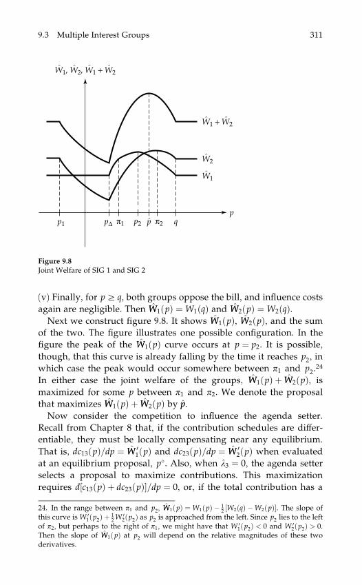
(v) Finally, for pb q, both groups oppose the bill, and influence costs

again are negligible. Then WW1ðpÞ ¼ W1ðqÞ and WW2ðpÞ ¼ W2ðqÞ.Next we construct figure 9.8. It shows WW1ðpÞ, WW2ðpÞ, and the sum

of the two. The figure illustrates one possible configuration. In the

figure the peak of the WW1ðpÞ curve occurs at p ¼ p2. It is possible,

though, that this curve is already falling by the time it reaches p2, in

which case the peak would occur somewhere between p1 and p2.24

In either case the joint welfare of the groups, WW1ðpÞ þ WW2ðpÞ, is

maximized for some p between p1 and p2. We denote the proposal

that maximizes WW1ðpÞ þ WW2ðpÞ by pp.

Now consider the competition to influence the agenda setter.

Recall from Chapter 8 that, if the contribution schedules are differ-

entiable, they must be locally compensating near any equilibrium.

That is, dc13ðpÞ=dp ¼ WW 01ðpÞ and dc23ðpÞ=dp ¼ WW 0

2ðpÞ when evaluated

at an equilibrium proposal, p�. Also, when l3 ¼ 0, the agenda setter

selects a proposal to maximize contributions. This maximization

requires d½c13ðpÞ þ dc23ðpÞ�=dp ¼ 0, or, if the total contribution has a

Figure 9.8

Joint Welfare of SIG 1 and SIG 2

24. In the range between p1 and p2, WW1ðpÞ ¼ W1ðpÞ � 12 ½W2ðqÞ �W2ðpÞ�. The slope of

this curve is W 01ðp2Þ þ 1

2W02ðp2Þ as p2 is approached from the left. Since p2 lies to the left

of p2, but perhaps to the right of p1, we might have that W 01ðp2Þ < 0 and W 0

2ðp2Þ > 0.Then the slope of WW1ðpÞ at p2 will depend on the relative magnitudes of these twoderivatives.


kink at some p, then d½c13ðpÞ þ dc23ðpÞ�=dp > 0 to the left of the kink

and d½c13ðpÞ þ dc23ðpÞ�=dp < 0 to the right of the kink.25 Together,

these observations imply that an equilibrium proposal must occur

where WW 01ðpÞ þ WW 0

2ðpÞ ¼ 0 or where WW1ðpÞ þ WW2ðpÞ has an upward

kink. In other words, an equilibrium proposal achieves a local maxi-

mum of the joint welfare of the two groups.

In figure 9.8 the joint welfare of SIG 1 and SIG 2 has local maxima

at pa p1, at pb q, and at p ¼ pp. However, no proposal of a policy

pa p1 or pb q can emerge as an equilibrium of the influence game.

To see this, suppose to the contrary that p is an equilibrium proposal

for some pa p1 or pb q. Since neither group prefers any such p to the

status quo policy, the policy outcome would be the status quo. Then

SIG 1 achieves expected welfare of W1ðqÞ, which is the worst possible

outcome for this group. It follows that SIG 1 would not contribute

positively to encourage the agenda setter to make such a proposal.

But if c�13ðpÞ ¼ 0, SIG 2 could offer the agenda setter a tiny amount to

propose its favorite policy p2, and the agenda setter would readily

oblige. Since SIG 2 prefers this outcome to the status quo, it would

never design a contribution schedule to induce the proposal p.

The unique equilibrium proposal is pp, the proposal that maximizes

WW1 þ WW2. For the example illustrated in figure 9.8, neither interest

group contributes anything to L1 or to L2 when the agenda setter

proposes pp. This is because p2 < pp < p2, so both groups prefer the

proposed policy to the status quo. The proposal pp, which passes the

legislature with probability one, maximizes the sum of the groups’ ex

ante utilities.26 The agenda setter is the only legislator who receives

campaign contributions in this case.27

25. Such a kink might occur at p2, if WW1ðpÞ slopes sharply downward to the right ofthat point.26. This statement presumes that W1ðpÞ þW2ðpÞ has a unique local maximum, as itmust when both functions are concave. This is true of the functions that underlie figure9.8.27. If we further assume that both groups use compensating contribution schedules, wecan calculate their equilibrium contributions. Were SIG 1 to be inactive at the proposalstage, SIG 2 would induce the agenda setter to set p�1 ¼ p2, and would pay virtuallynothing to L3. This would yield SIG 2 a utility of W2ðp2Þ. Therefore, according to theanalysis presented in Chapter 8, SIG 1 pays c�13 ¼ W2ðp2Þ �W2ð ppÞ to the agenda setter ina compensating equilibrium. Similarly, if SIG 2 were to be inactive at the proposal stage,SIG 1 would induce the agenda setter to set p�2 ¼ p2 for the case illustrated in figure 9.8.The group prefers this policy to its overall ideal, because the latter would requiregreater contributions in the second stage and its legislative prospects would remaindim. The contributions from SIG 2 to the agenda setter must compensate for the sur-plus that SIG 1 otherwise could achieve. Therefore, c�23 ¼ W1ðp2Þ �W1ð ppÞ.


As we have indicated, it is also possible that WW1ð�Þ peaks at a pro-

posal between p1 and p2. Then the joint-welfare-maximizing proposal

pp may fall between p1 and p2. Such a pp again would be the unique

equilibrium proposal when the agenda setter seeks to maximize

contributions. In such a case, WW 01ðpÞ þ WW 0

2ðpÞ ¼ 0 implies W 01ðpÞ þ

32W

02ðpÞ ¼ 0, considering that WW1ðpÞ ¼ W1ðpÞ � 1

2 ½W2ðqÞ �W2ðpÞ� andWW2ðpÞ ¼ W2ðpÞ for proposals in this range. So the equilibrium pro-

posal in this case is not the one that maximizes the sum W1ðpÞ þW2ðpÞ, but rather one that puts more weight on the policy prefer-

ences of SIG 2. Of course, SIG 2 pays for this privilege, not only to

the agenda setter but also to the remaining legislators. In fact, at the

voting stage, SIG 2 opposes the proposed legislation, and offers a

random amount to L1 and L2 in an effort to engineer its defeat. The

bill’s fate remains uncertain, which means that there is a positive

probability that the status quo will persist. Because the inefficient

status quo prevails with positive probability, and because the pro-

posed alternative does not maximize W1ðpÞ þW2ðpÞ, the equilibrium

outcome is not jointly efficient for the interest groups and the

legislators.

Now that we understand the political pressures on the agenda

setter, we can allow for his policy preferences. The agenda setter

chooses the proposal that maximizes GL3 ¼ l3WWL3ðpÞ þ ð1� l3Þ �½c13ðpÞ þ c23ðpÞ� where WWL3ðpÞ is his expected welfare in the voting

stage. Observe that the agenda setter must consider not only whether

a policy meets his political objectives, but also whether it has a rea-

sonable chance to succeed. Thus,

WWL3ðpÞ ¼ Pr½p succeeds� �WL3ðpÞ þ Pr½p fails� �WL3ðqÞ:

When the contribution schedules are locally compensating, the

candidates for equilibrium are those proposals that achieve a local

maximum of l3WWL3ðpÞ þ ð1� l3Þ½WW1ðpÞ þ WW2ðpÞ�.Take, for example, a case where the agenda setter has a favorite

policy of pL3 and single-peaked policy preferences. Consider the

proposal pp that maximizes WW1ðpÞ þ WW2ðpÞ. If p2 < pp < p2, as in figure

9.8, then the proposal pp and others close to it would succeed in the

legislature with probability one. Then, if pL3 < pp, there is an equilib-

rium in which the agenda setter proposes a policy to the left of pp,

whereas if pL3 > pp, there is an equilibrium in which the agenda setter

proposes a policy to the right of pp. Alternatively, ppmight fall between

p1 and p2. Then the success of pp and other similar proposals is not


ensured. Proposals to the right of pp stand a better chance of success

than pp itself, whereas those to the left of pp are more likely to fail. If

pL3 > pp, both the agenda setter’s preferences and the legislative real-

ties point to his choosing something to the right of pp. But if pL3 < pp,

these forces push in opposite directions, and it is not clear which one

is stronger.

All of this may be clearer in the following example.

9.3.3 The Scale of a Public Project

Imagine a legislature that must decide whether to proceed with an

important public project, and if so, at what scale. There are two

interest groups in society. One stands much to gain from the project,

while the other would also benefit from the undertaking but to a

lesser extent. For SIG 1, W1ðpÞ ¼ 36p� 12 p

2, where W1ðpÞ represents

the group’s utility from a project of size p net of its share of the con-

struction cost. As for SIG 2, W2ðpÞ ¼ 6p� 12 p

2. With these prefer-

ences, p1 ¼ 36 and p2 ¼ 6. Of course, the groups seek to maximize

their welfare net of any contributions, which are c1 and c2, respec-

tively. The project has no other sources of funding, so the status quo

is q ¼ 0.

Both groups prefer small projects to the status quo. Since legis-

lators L1 and L2 care only about contributions, any bill calling for

p < 12 would be passed in the legislature at virtually no cost to the

groups. But SIG 2 would oppose any project with p > p2 ¼ 12, as can

be seen in figure 9.9. Thus, for any p < p1 ¼ 72, there would be con-

flict between the groups. The conflict would be resolved in favor of

SIG 2, if �DD2 > 2D1. This spells sure defeat for any bill calling for

p > pD ¼ 52. For proposed projects with scales between 12 and 52,

the groups would randomize their offers, leaving the legislative

prospects for any such bill uncertain. The probability of passage

declines as the proposed scale grows larger in this range.

Now consider the groups’ efforts to influence the agenda setter.

Suppose first that the agenda setter cares only about campaign

contributions. For 12a pa 52, the expected welfare for SIG 1 net of

contributions is WW1ðpÞ ¼ W1ðpÞ � 12 ½W2ðqÞ �W2ðpÞ�. In this range,

WW2ðpÞ ¼ W2ðpÞ. Thus, WW1ðpÞ þ WW2ðpÞ ¼ W1ðpÞ þ 32W2ðpÞ ¼ 45p� 5

4 p2,

in view of the fact that q ¼ 0 implies W2ðqÞ ¼ 0. This function—which

represents the joint welfare of the SIGs at the voting stage—reaches a

maximum at p ¼ 18. So this is the equilibrium proposal as we saw in


the previous section. The agenda setter determines his proposal in

response to the opposing incentives provided by the two interest

groups. The agenda setter could obtain more contributions from SIG

1 by increasing the scale of the project, and more from SIG 2 by

scaling it back. On the margin, the offsetting incentives balance, and

the agenda setter maximizes his contributions by proposing p ¼ 18.

Once the equilibrium bill has been drafted, the objectives of the

two SIGs conflict. SIG 1 would like to see the bill passed by the leg-

islature, whereas SIG 2 prefers the status quo. In the equilibrium, the

groups randomize their contribution offers to L1 and L2. SIG 1 offers

a contribution to only one of these legislators, hoping to encourage a

single additional positive vote. The group targets L1 and L2 with

equal probability, and offers a positive contribution that is no more

than �DD2=2 ¼ 27. SIG 2 offers the same contribution to both legislators,

but the offers may be zero. In fact, the group makes no (positive)

offers with probability 1� �DD2=2D1 ¼ 17=18. Using the equation in

footnote 21, we can calculate the probability that the bill will pass.

We find that it does so with a probability of almost 98 percent.

If we further assume that the two groups design compensating

contribution schedules, we can calculate the (actual or expected)

contribution that each makes to the three legislators. In a compen-

sating equilibrium, SIG 1 pays the agenda setter c13 ¼ 261. This is the

Figure 9.9

Conflicting SIG Tastes for a Public Project


difference between the group’s expected welfare of WW1ð18Þ ¼ 459 at

the start of the voting phase and the expected welfare of WW1ð6Þ ¼ 198

that it would achieve if the proposal were instead p�1 ¼ 6. A project

of size 6 maximizes WW2ðpÞ and therefore is the one that SIG 2 would

pick if SIG 1 did not participate in the first-stage game. Similarly, SIG

2 pays the agenda setter c23 ¼ 128 in the compensating equilibrium.

This is the difference between its expected welfare of WW2ð18Þ ¼ �54

and the lower expected welfare of WW2ð26Þ ¼ �182 it would suffer if

SIG 1 were to induce a proposal of p�2 ¼ 26.

At the voting stage, SIG 1 pays an expected contribution of 382,

which goes to either L1 or L2 with equal probability. SIG 2 pays

expected contributions totaling approximately 1.2. Half of this sum

goes to each of L1 and L2.28

Now suppose the agenda setter has policy preferences of his own.

We take WL3ðpÞ ¼ 24p� 12 p

2, so that the agenda setter has an ideal

project of pL3 ¼ 24. Let the agenda setter place equal weight on the

policy outcome and campaign contributions, that is, l3 ¼ 12.

Without contributions, the agenda setter would propose pF 22:5,

which is the policy that maximizes WWL3ðpÞ. This proposal is a bit less

than his personal favorite of p ¼ 24, because he recognizes that the

smaller project has a better chance of succeeding in the legislature.

But the joint influence of SIG 1 and SIG 2 causes the agenda setter to

propose a project even smaller than this. The equilibrium proposal is

the one that maximizes l3WWL3ðpÞ þ ð1� l3Þ½WW1ðpÞ þ WW2ðpÞ�. We cal-

culate that p� F 19:3 and that this proposal passes in the legislature

with a probability of approximately 97 percent.

In this example, the equilibrium proposal by an agenda setter who

himself covets a project of p ¼ 24 is larger than the proposal that

would be made by an agenda setter who does not care about the size

of the project at all. This is not surprising, because the agenda setter’s

ideal scale exceeds the size of the project that would be proposed by

an agenda setter who sought only contributions. It is worth empha-

sizing, though, that the equilibrium proposal need not fall between

the agenda setter’s own ideal policy and the proposal that would

result were the agenda setter not to care about the policy outcome.

Take, for example, a case where the agenda setter’s policy preferences

are given by WL3ðpÞ ¼ 18:1p� 12 p

2. In this case, his favorite project is

28. These expected contributions can be calculated using the distribution functions ofthe offers, (9.5) and (9.6), recognizing that the contributions are paid only when agroup’s offer to L1 or L2 is the largest.


pL3 ¼ 18:1, which exceeds the size of the equilibrium proposal that

results when lL3 ¼ 0. But the equilibrium proposal is p� ¼ 17:8. The

equilibrium proposal does not lie between 18 and 18.1, but it does

lie between 18 and the proposal that the agenda setter would make if

he encountered no bids for influence. The proposal that maximizes

WWL3ðpÞ has pF 17:4, a scale that is smaller than the agenda setter’s

ideal, because he factors in the legislative realities. The contribution

offers cause him to propose a project slightly bigger than this, but not

so big as the one that would result were his own preferences to play

no role.

In this chapter, we have extended the analysis of influence seeking

by SIGs to settings in which policy decisions are made by groups of

policymakers acting as a legislature. If party discipline is strong, so

that individual legislators invariably vote with their party leaders,

then a legislature can be regarded as a single actor, and the analysis

presented in Chapters 7 and 8 applies. But in many polities, party

dictums are not inviolable. Then a SIG that wishes to influence policy

must consider the legislative process. It may wish, for example, to

curry favor with those who will decide the contents of a bill, instead

of or in addition to those who will determine its fate.

We have illustrated how a legislature may be influenced by special

interests, using one particularly simple specification of the legislative

process. In this specification, an agenda setter determines the content

of a bill, which then stands in opposition to a given status quo. This

example mostly is meant to point the way forward. Different legis-

latures follow a variety of rules for determining what bills are

reported to the floor, how amendments are offered, and how the

voting proceeds. Further research is needed to understand how these

different rules affect the influence of special interests and to identify

which rules best serve the general public.


10 Contributions andElections

The previous three chapters focused on campaign contributions. We

have tried to capture the tension that many elected officials feel be-

tween serving their constituents and raising vitally needed campaign

funds. Our approach has been to include policy outcomes and cam-

paign contributions as separate arguments in the policymaker’s objec-

tive function. In so doing, we have treated the politicians’ motivations

in reduced form, with an allusion to electoral considerations but

without a full-fledged model of voting behavior and rival candidates.

While useful for highlighting the interaction between politicians

and interest groups, the reduced-form approach has several short-

comings. It does not allow one to say anything about how policy out-

comes matter to a politician who is driven by a desire to be reelected.

Nor can it shed any light on what determines the perceived trade-off

between policies and money. Moreover, it is not at all clear that a

policymaker’s concern for policies or her taste for contributions is

invariant to the electoral context. Voters may be more forgiving of a

politician who advocates certain policies if they expect her rival

would do the same or worse. Campaign resources may be more

valuable to an unknown or unpopular candidate than to one who is

already well liked or one who faces a weak opponent. None of these

considerations can be addressed in a model that puts voting behav-

ior off to the side.

There is another reason why we may wish to study campaign

giving and voting together. Until now, we have considered only one

of the possible motivations that interest groups have for contributing

to political campaigns.1 We have focused exclusively on the influence

1. Actually, in Chapter 5 we also discussed the use of campaign giving as a means togain access to a less than perfectly informed policymaker and as a way for a group tosignal its private information.

motive, according to which groups give to candidates or parties in the

hope of influencing their positions and the policies they enact. Some

political scientists question the importance of this explanation for

campaign giving, attributing instead an electoral motive to virtually

all contributors.2 According to this view, SIGs regard the positions

and intentions of most politicians as inviable. They contribute to the

candidates whose positions they like so as to enhance their prospects

for winning the election. In order to understand the conditions under

which each of the motives for campaign giving is operative, and to

assess whether they work in tandem or in conflict, we need a model

in which the relationship between campaign spending and election

outcomes is made explicit.

In this chapter we will modify our earlier modeling of electoral

competition to allow a role for campaign spending. As before, we

examine a single electoral contest between two political parties. The

election will determine the outcome of some fixed and some pliable

policy issues. The parties’ stances on the fixed issues are given from

the outset, but the parties take positions on the pliable issues to fur-

ther their electoral objectives. By adopting a certain position, a party

commits to carry out the indicated policies if it should win the elec-

tion. Strategic voters, as before, consider only the pair of platforms

when deciding how to cast their ballots. But we introduce a second

category of impressionable voters who pay heed to campaign adver-

tising. These voters are the targets of the campaign spending, which

is funded by donations from interest groups. A group may tie its

donation to the positions that a party takes or grant the donation

unconditionally. In this sense, a SIG may be guided by either an

influence motive or an electoral motive (or both) in determining the

size of its campaign gift.

The analysis in this chapter serves several purposes. It provides a

rigorous underpinning for the reduced-form approach that we used

2. As we have noted before, many SIGs contribute primarily to politicians who arepredisposed to their own positions. Some take this observation as evidence that cam-paign gifts are not meant to curry favor. But other evidence—of especially large con-tributions by certain industries to members of certain committees, of contributions bythe same PAC to opposing candidates and parties, and of changes in giving when arepresentatitive is transferred to a new committee—points in the opposite direction.Moreover, gifts to like-minded politicians may have influence as their motive, if theyare intended not to buy a vote but rather to encourage the recipient to play an activerole in drafting or amending a bill, or perhaps to engage in log-rolling with otherrepresentatives who are not similarly inclined.

320 Contributions and Elections

in Chapters 7 through 9, and it allows us to examine the determinants

of a politician’s willingness to trade off welfare for contributions. The

expanded framework also enables us to weigh the different motives

that interest groups have for engaging in campaign giving. Finally, it

provides explanations for two common observations about political

giving: namely, many SIGs contribute to both contestants in the

same election, and patterns of giving are heavily skewed toward

favorites relative to underdogs.3

10.1 Electoral Competition with Campaign Spending

Recall the electoral model of Chapters 2 and 3.4 There are two

political parties, each with fixed positions on some set of issues. The

parties choose their positions on the remaining issues so as to maxi-

mize their chances of winning a majority of the votes. The parties

are committed to carry out their platforms in the event they emerge

victorious. Voters belong to identifiable groups, indexed by j. The

members of group j share a common interest in the pliable issues but

hold different views on the fixed issues.

10.1.1 The Voters

We extend the earlier model to include two categories of voters.

Strategic voters understand the political environment and the impli-

cations of their votes. Each such voter recognizes that his vote will

increase slightly the subjective probability that the party he has

named will be victorious. A voter’s uncertainty reflects his imperfect

information about the aggregate popularity of the two parties. By

voting for the party whose platform he prefers, a strategic voter

slightly raises his expected welfare. This is a dominant strategy for

him.

Impressionable voters, in contrast, are receptive to the messages of

the political campaign. Perhaps these voters do not deem it worth-

3. Snyder (1990) has presented evidence that, in open-seat races for the U.S. Congress,campaign spending varies in proportion to a candidate’s probability of being elected.The often noted bias in contributions toward incumbent candidates can also be un-derstood in these terms, once we recognize that most incumbents are heavily favoredin their bids for reelection.4. We used a similar model in Chapter 6, except that there we assumed voters areunsure of the connection between the policy variable and their own welfare.


while to make the calculations necessary for strategic voting. Or

perhaps the campaign ads provide them with bits of credible evi-

dence about a party’s competence or its rival’s incompetence. In any

case, we assume that impressionable voters respond to campaign

spending.5 The more a party spends (holding constant the spending

of its rival), the greater is its share of the impressionable votes.6

Let us focus first on the behavior of strategic voters. This discus-

sion should be familiar by now.7 The strategic voter i in group j has

the utility function ujðpkÞ þ vkij, where pk is the vector of pliable

policy outcomes and vkij is the voter’s utility from the fixed positions

of party k, k ¼ A;B. Note that the first component depends only on

the group to which the individual belongs, whereas the second

component varies across individuals in the same group. We again let

vij ¼ vBij � vA

ij denote the relative preference of voter i in group j for

the fixed positions of party B. We assume that vij has the same uni-

form distribution in all interest groups, with a mean of b=f and a

density of f . The mean of the distribution indicates which party’s

ideology is more popular among strategic voters and by how much.

Specifically, the greater is b, the greater is the fraction of strategic

voters that prefer the fixed policy positions of party B.

The strategic voter i in group j votes for party A if and only if

vij a ujðpAÞ � ujðpBÞ. Considering that vij is distributed uniformly

5. The available evidence supports the view that campaign spending wins votes.Jacobson (1980, 1985) has argued that in U.S. congressional elections, campaignspending is effective only for challengers, not for incumbents. But after controlling forthe quality of challengers and the endogeneity of various regressors, Green and Krasno(1988) found significant marginal vote gains from spending for both challengers andincumbents. More recently, Gerber (1998) has produced additional evidence for U.S.senatorial races that supports the Green-Krasno position.6. We follow Baron (1994) in treating the productivity of campaign spending inreduced form. In contrast, Austen-Smith (1987) has modeled informative advertisingthat reduces voters’ uncertainty about the candidates’ positions. Potters, Sloof, andvan Winden (1997) and Prat (2001) study models in which campaign spending isindirectly informative. In Prat’s model, for example, the SIGs have better informationthan voters about the competence of the incumbent candidate. The level of his cam-paign spending signals his competence, because the SIGs are more willing to contrib-ute to the incumbent the better they regard his chances of being reelected. Prat doesnot allow for contributions to the challenger, but a suitably extended version of hismodel could be used to justify our treatment of the effectiveness of campaign spendingin a setting with only strategic voters.7. We highlight one difference from Chapters 3 and 6. There we assumed that a voter’sutility from the pliable policy declines with the square of the difference between thatpolicy and the voter’s ideal policy level. Here, as in Chapter 2, we allow for a vector ofpliable policies and do not impose any functional form on the utility function.


with mean b=f and density f , this implies that a fraction

sSj ¼ 12 � bþ f ½ujðpAÞ � ujðpBÞ�

of the strategic voters in group j vote for party A. Notice that if

pA ¼ pB, then sSj ¼ 12 � b; when pliable platforms are the same, the

votes divide according to the popularity of the parties. We assume

that f is small enough that sSj falls between zero and one for all fea-

sible policy options.

We can take a weighted sum of the vote shares in the various

groups to compute the fraction of all strategic votes that go to party

A. The appropriate weights are the shares of each group in the total

number of strategic voters. Let Nj be the number (measure) of voters

in group j and let N ¼P

j Nj be the total size of the electorate. We

treat the fraction of strategic voters in each group as exogenous and

common to the groups; for future reference, we denote it by m.8

Forming the weighted sum, we find that the fraction of the strategic

votes cast for party A is

sS ¼ 12 � bþ f ½uðpAÞ � uðpBÞ�; ð10:1Þ

where uðpkÞ ¼P

j NjujðpkÞ=N is the average utility component asso-

ciated with the pliable policies of party k in the population of all

strategic voters.

Now consider the impressionable voters. These individuals account

for a fraction 1� m of the members of each group. For simplicity, we

do not derive the voting behavior of these individuals from first

principles. Rather, we assume that the fraction of them who vote for

each party reflects the popularity of the fixed positions of each party

and the difference in campaign spending. A fraction

sIj ¼ 12 � bþ eðcA � cBÞ

of the impressionable voters in group j votes for party A when this

party spends cA on the campaign and its rival spends cB. Implicit in

this specification is the assumption that, all else being equal, the

parties enjoy the same popularity among impressionable voters as

they do among strategic voters. Since the same fraction of impres-

8. It would be straightforward to allow the fraction of strategic voters to vary bygroup. This would introduce an additional bias in policies that is similar to the biascaused by differential turnout, as discussed in Chapter 3, Section 3.1. Here we wish toemphasize the role of competing campaign contributions, which is easier to see whenthe fraction of impressionable voters is the same in every group.


sionable voters votes for party A in every group, we have that

sI ¼ 12 � bþ eðcA � cBÞ; ð10:2Þ

where sI is party A’s vote share among all impressionable voters.

Finally, we can weight sS and sI respectively by the shares of stra-

tegic and impressionable voters in the voting population, and sum

the two terms. This gives the overall share of the votes that goes to

party A. Using (10.1) and (10.2), we have

s ¼ 12 � bþ m f ½uðpAÞ � uðpBÞ� þ ð1� mÞeðcA � cBÞ; ð10:3Þ

where s is the total vote share for party A.

10.1.2 The Parties

Each party must announce its positions on the pliable issues before

it learns the relative popularity of its fixed positions. That is, at the

time that pA and pB are chosen, each party regards b as the future

realization of a random variable ~bb. Ex ante, b can be positive or neg-

ative, so that even if the pliable platforms converge, each party has a

chance to win a majority. We again use Fbð�Þ to denote the distribu-

tion of ~bb as perceived by the parties at the time they adopt their

positions. Each party sets its platform to maximize its chance of

winning a majority, in light of its prior beliefs about the distribution

of ~bb.

To establish a benchmark, let us first consider a setting with m ¼ 1,

so that all voters are strategic. In this case the parties have no pro-

ductive use for campaign funds. Party A chooses pA to maximize

the probability that s > 12, which is Fbf f ½uðpAÞ � uðpBÞ�g. Since Fbð�Þ

is an increasing function, the party maximizes its prospects for a

victory by choosing the platform that maximizes uðpÞ. Similarly,

party B chooses pB to maximize the probability that s < 12, which is

1� Fbf f ½uðpAÞ � uðpBÞ�g. This party too sets its pliable platform to

maximize the welfare of the average voter. Thus, the pliable policies

that emerge are the same no matter which party wins the election.

Without impressionable voters, our model predicts a pliable policy

outcome that is not biased toward the preferences of any group.

When m < 1, campaign spending produces votes. Therefore, the

parties do not ignore their campaign finances when choosing their

pliable positions. Recall that the SIGs may link their contributions to

the policy platforms. Let CAj ðpAÞ be the contribution schedule offered


by SIG j to party A as a function of that party’s campaign announce-

ments. Similarly, let CBj ðpBÞ be the offer by SIG j to party B. The

party’s total contributions are

cA ¼Xj

CAj ðpAÞ ð10:4Þ

and

cB ¼Xj

CBj ðpBÞ; ð10:5Þ

respectively. Substituting (10.4) and (10.5) into (10.3), we can compute

the objective of each party. For party A, the probability that s > 12 is

greatest when the party adopts the pliable platform that maximizes

GA ¼ m fuðpAÞ þ ð1� mÞeXj

CAj ðp

AÞ: ð10:6Þ

For party B, the optimal platform is the one that maximizes the

probability that s < 12, which implies that the party should maximize

GB ¼ m fuðpBÞ þ ð1� mÞeXj

CBj ðp

BÞ: ð10:7Þ

Notice that the parties have similar objectives, namely, to maxi-

mize a weighted sum of campaign contributions and the welfare of

strategic voters. Of course, this objective is exactly what we took to

be the policymaker’s welfare function in Chapters 7 and 8. Here the

incentives in the electoral contest determine the relative weights. The

parties attach a greater weight to welfare, the greater is the fraction

of strategic voters (the larger is m) and the more narrow is the range

of their views on the ideological issue (the larger is f ). This is intuitive.

The strategic voters are the ones who compare the pliable positions

when deciding how to vote. The more numerous they are, the more

attention their preferences will receive from the competing parties.

Also, when their ideological perspectives are diverse, there are rela-

tively few of them who will change their votes in response to a

given change in a party’s position. Then the parties have relatively

little incentive to cater to their interests in setting their platforms.

The weight on campaign contributions increases with the fraction of

impressionable voters and with the effectiveness of campaign spend-

ing. When e is large, a small increase in spending can be used to win


over a large number of impressionable voters. In such circumstances,

campaign finances weigh heavily in the strategies of the two parties.

10.1.3 The Interest Groups

The organized interest groups promote the policy objectives of their

members. As in Chapter 6, the leaders of a SIG might have either a

narrow mandate to pursue only their members’ common objectives

in regard to the pliable policies or a broader mandate to pursue total

welfare from both the fixed and pliable policies. Here, to keep matters

simple, we suppose that the mandate is narrow. We take the objective

function for the leaders of an organized SIG j to be E½Njujð~ppÞ� � cj,

where cj ¼ cAj þ cBj is the sum total of the group’s campaign contri-

butions and ~pp is the vector of policies enacted by the party that wins.

The expectation reflects the group’s uncertainty about who will win

the election.

The SIGs formulate their contribution offers before the policy posi-

tions have been chosen. This means that the contribution schedules

are designed before the relative popularity of the parties is known.

Each SIG takes the contribution schedules of its rivals as given. It

forms an expectation of the probability that each party will win the

election and calculates its optimal contributions accordingly.

The SIGs anticipate the pliable positions that the parties will

choose in response to any contribution schedule they might design,

and given the schedules they expect their rivals to offer. With this

anticipation, a group can calculate the implied probabilities of a

victory by each side. Specifically, the SIG knows that party A will

win a majority if and only if the realization of ~bb is such that s > 12.

This happens with probability FbðDÞ, where from (10.6) and (10.7),

D ¼ GA � GB ¼ m f ½uðpAÞ � uðpBÞ� þ ð1� mÞeðcA � cBÞ: ð10:8Þ

So, in evaluating its objective function, the group attaches a proba-

bility FbðDÞ to the event that p ¼ pA, and a probability 1� FbðDÞ to

the event that p ¼ pB. Accordingly, we can rewrite its objective

function as

Uj ¼ FbðDÞNjujðpAÞ þ ½1� FbðDÞ�NjujðpBÞ � cAj � cBj : ð10:9Þ

We can approach the problem facing SIG j as we did in Chapter 8.

First, the leaders of a SIG contemplate what pliable platforms would


be best for their members, considering the incentives facing the polit-

ical parties. Then they consider what platforms would result in the

absence of any contributions of their own. Finally, they design a pair

of contribution schedules to implement their preferred positions,

bearing in mind the constraints imposed by the fact that a party need

not accept the group’s offer of support. Notice that a SIG may well

choose to contribute to both sides in the election. Since there is a

positive probability that either platform will be enacted, the SIG has

reason to try to influence the positions taken by both parties.

In order to proceed, we need some additional notation. Let pA�j and

pB�j be the platforms that the two parties would adopt in the absence

of any contributions from SIG j. These are the platforms that maxi-

mize GA and GB respectively, but with CAj ðpAÞ and CB

j ðpBÞ set iden-tically equal to zero. Now let GA

�j and GB�j denote the levels of GA and

GB that the parties would achieve under these circumstances.9 The

problem facing SIG j is to select policies pAj and pB

j and contribution

levels cAj and cBj to maximize its objective in (10.9), subject to the

constraints that GA bGA�j and GB bGB

�j.

We will be interested in whether the constraints GA bGA�j and

GB bGB�j are binding in equilibrium. If GA ¼ GA

�j; it means that party

A is just indifferent between announcing the platform pAj preferred

by SIG j (preferred, that is, in light of the offers to party A by other

interest groups) and ignoring the group’s offer altogether. The party’s

indifference implies that it has the same probability of victory when

the offer is accepted as when it is declined. Accordingly, the gift from

SIG j does not improve the party’s electoral prospects under such

circumstances. Then the motivation for SIG j in giving to party A

could only be to influence its policy positions. If GA ¼ GA�j in the

equilibrium, we will say that SIG j has exercised only an influence

motive for contributing to party A.

In contrast, when GA > GA�j in equilibrium, it means that SIG j is

giving to party A more than the minimal amount needed to influence

9. More formally,

p k�j ¼ arg max

pm fuðpÞ þ ð1� mÞe

Xljl0j

Ckl ðpÞ

and

Gk�j ¼ m f uðp k

�jÞ þ ð1� mÞ fXljl0j

Ckl ðp k

�jÞ

for k ¼ A;B.


its platform. The only reason the group could have for such gener-

osity is to enhance the party’s prospects for electoral success. In case

of a nonbinding constraint, we will say that the interest group has

exercised an electoral motive for campaign giving.

An equilibrium arises when the pair of contribution schedules for

each organized SIG are mutual best responses in light of the antici-

pated outcome at the platform-setting stage. The platform choices

must also be best responses to the contribution schedules.

10.2 One Interest Group

In this section we examine electoral competition in a setting in which

only a single interest group is politically organized. First, we hypoth-

esize that the group gives only to influence the parties’ positions and

derive some of the implications that follow from this assumption.

Then we alter the game so that the group has no chance to exert

influence. This allows us to examine a pure electoral motive for

campaign giving. Finally, we study the general case in which a

group may contribute for either or both reasons. We ask, When does

each motive operate, and what effect do the optimal contributions

have on the policy positions and the election odds?

10.2.1 The Influence Motive

Suppose there is only one active interest group, denoted by j. The

group can contribute to one or both of the political parties. In this

section, we hypothesize that only the influence motive operates. That

is, the SIG gives to each party, if anything, exactly what is needed to

induce the party to choose the prescribed platform. We will examine

the validity of this hypothesis in Section 10.2.3 below.

When only one SIG contributes to the political parties, they have no

alternative sources of campaign funding. This makes it easy to com-

pute pA�j and pB

�j, the positions that each would take in the absence of

contributions from the group. If SIG j were to offer nothing to party

A, the party would maximize its probability of winning by choosing

pA to maximize uðpÞ. Party B would likewise announce the platform

that maximizes uðpÞ. So pA�j ¼ pB

�j ¼ p�, where p� denotes the policy

vector that maximizes the welfare of the average strategic voter.

These best alternatives give the parties reservation utility levels of

GA�j ¼ GB

�j ¼ m fuðp�Þ.


If the interest group wishes to have a party take a position differ-

ent from p�, it must compensate the party for the loss of votes that

such an announcement would imply. To make party A indifferent

between announcing p� and some other platform pA, the group must

contribute

cAj ¼ m f

ð1� mÞe ½uðp�Þ � uðpAÞ�: ð10:10Þ

Similarly, an announcement of pB by party B would cost the group

cBj ¼ m f

ð1� mÞe ½uðp�Þ � uðpBÞ�: ð10:11Þ

In each case, the contribution leaves the party with the same chance

of winning the election as it would have without any campaign

spending. But if spending by both parties were zero, they would

choose identical pliable platforms of p�, and party A would win the

election with probability Fbð0Þ. It follows that this too is the proba-

bility of an electoral victory by party A no matter what pair of plat-

forms the SIG decides to pursue.

The problem facing the leaders of the SIG is to choose pA and pB to

maximize the members’ expected welfare from the pliable policy

outcome net of campaign contributions. Using (10.10) and (10.11), we

can rewrite the organization’s objective function, (10.9), as

Fbð0ÞNjujðpAÞ þ ½1� Fbð0Þ�NjujðpBÞ � m f

ð1� mÞe ½2uðp�Þ � uðpAÞ � uðpBÞ�:

Then the solution implies

pA ¼ arg maxp

Fbð0ÞNjujðpÞ þm f

ð1� mÞe uðpÞ� �

ð10:12Þ

and

pB ¼ arg maxp

½1� Fbð0Þ�NjujðpÞ þm f

ð1� mÞe uðpÞ� �

: ð10:13Þ

The SIG induces each party to announce a platform that maximizes

a weighted sum of the members’ aggregate welfare from the pliable

policies, NjujðpÞ, and the utility component for the average strategic

voter, uðpÞ. The relative weight that either party attaches to SIG

members depends on the ex ante probability that the party will

prove to be the more popular, Fbð0Þ for party A and 1� Fbð0Þ for


party B. The more popular a party is likely to be, the greater is the

bias in its pliable platform.

The influence motive inclines the SIG to give to both political

parties. Since even the underdog may emerge as the winner of the

election, the SIG has reason to guard itself against the possibility that

this party’s platform will become the law. The group must pay to

influence each platform. But the cost to the group of inducing a small

departure from a party’s best alternative is quite small. This follows

from the fact that the best alternative positions maximize uðpÞ. By the

properties of a maximum, a small departure from p� does not reduce

uðpÞ by very much and so does not cost a party many votes. There-

fore, the compensation that is needed for the SIG to buy the first bit

of influence is negligible.

Although the SIG exerts its influence on both platforms, it does not

contribute equally to the two parties. Rather, it gives more to the

party that is more likely to win the election. This can be seen by

comparing (10.12) and (10.13). The comparison shows that the front-

runner ultimately gives relatively more weight to SIG members and

less weight to strategic voters. In order to induce the front-runner to

pay less attention to the interests of strategic voters, the SIG must

give more to this party by way of compensation (see equations

(10.10) and (10.11)).

It is easy to understand why an influence-motivated SIG would

give more generously to the electoral favorite. Political contributions

are an investment that pays off for the SIG only if the recipient wins

the election. Since the electoral favorite has a better chance of win-

ning, an investment in this party is more likely to yield a positive

return. Accordingly, the SIG invests more to influence the favorite

than the underdog. This prediction of the model is consistent with

the evidence on campaign giving presented by Snyder (1990). It also

helps to explain why incumbents, who typically are heavily favored

in their bids for reelection, often raise more in contributions from

interest groups than their opponents do.

Let us conclude this section with some observations about the

extent of the bias in the pliable policies. If only an influence motive

operates, then with probability Fbð0Þ the realized policy outcome

is pA and with probability 1� Fbð0Þ it is pB, where pA and pB are

given in (10.12) and (10.13), respectively. In either case the size of the

policy bias is larger, the greater is the effectiveness of campaign

spending, the greater is the fraction of impressionable voters, and the


greater is the dispersion of views on the ideological issues. When

campaign spending is more effective, the parties are more willing

to trade off popular positions on the pliable policies for increased

campaign funding. This makes influence cheaper to buy. Similarly,

an increase in the fraction of impressionable voters raises the party’s

demands for campaign funds and lowers the price of influence. A

large spread of views on the fixed issues means a low sensitivity

of the vote totals to a change in the pliable policies, and thus a low

political cost to the parties of departing from p�. Again, this reduces

the price of influence.

10.2.2 A Pure Electoral Motive

In this section, we begin to investigate the electoral motive for cam-

paign giving. In order to best understand what is different about this

alternative reason for contributing, we make a temporary modifica-

tion to our model. For the time being, we assume that the SIG can

offer contributions to the parties only after they have announced

their positions on the pliable issues. With this timing, there is no

possibility for the SIG to influence the parties’ platforms. Rather, the

SIG can only hope to alter the probabilities that either side will win

the election.10

Consider first the incentives facing the leaders of the interest

group. By the time they must decide on their contributions, they will

know the parties’ positions on the pliable issues. The leaders will

know that if they contribute cAj to party A and cBj to party B, then

party A will win a majority of the votes if and only if b < D, where D

is given in (10.8). This will happen with probability FbðDÞ. The leaderschoose the group’s contributions to maximize the members’ expected

welfare from the pliable policies net of the payments; that is, they

maximize Uj given in (10.9).

It is obvious that, unlike the influence-motivated SIG, the elector-

ally motivated SIG contributes to at most one party. If it contributes

to party A, it increases D and thus the probability that party A will

win the election. If it contributes to party B, it does just the opposite.

But the leaders will only wish to further the electoral prospects of

10. Austen-Smith (1987) and Magee, Brock, and Young (1989) have studied models ofelectorally motivated campaign contributions in which the order of moves is as speci-fied here. Austen-Smith investigated the provision of public goods, whereas Mageeet al. focused on the determination of trade policies.


one party, namely the one whose pliable positions the members

prefer. Therefore, only this party is a candidate to receive the group’s

electorally motivated gifts.

Suppose, for concreteness, that ujðpAÞ > ujðpBÞ. Will SIG j neces-

sarily contribute to party A? The answer is no. The group perceives

a marginal benefit from its first dollar of contribution equal to

F 0bðD0Þð1� mÞeNj½ujðpAÞ � ujðpBÞ�, where D0 ¼ m f ½uðpAÞ � uðpBÞ�. This

benefit reflects the marginal effectiveness of the first bit of campaign

spending by party A in improving its chances of victory, and also

the extent of the members’ preference for pA over pB. The cost of

the dollar of contributions is, of course, one. The group will make a

positive contribution if the marginal benefit exceeds the marginal

cost, or if11

F 0bðD0Þð1� mÞeNj½ujðpAÞ � ujðpBÞ� > 1: ð10:14Þ

But there is no guarantee that this condition will be satisfied. More-

over, it can never be satisfied if the parties’ pliable positions are the

same. An electoral motive is more likely to operate the greater is the

difference in the group’s evaluation of the parties’ positions and

the more productive is campaign spending in generating votes.

If inequality (10.14) is satisfied, SIG j will contribute to party A.

The size of its gift will be such that the marginal benefit of the last

dollar of contribution matches the marginal cost, or

F 0bðDÞð1� mÞeNj½ujðpAÞ � ujðpBÞ� ¼ 1: ð10:15Þ

Similarly, if F 0bðD0Þð1� mÞeNj½ujðpBÞ � ujðpAÞ� > 1, the group will con-

tribute to party B, and cBj will be chosen so that

F 0bðDÞð1� mÞeNj½ujðpBÞ � ujðpAÞ� ¼ 1:

To summarize, there are two important lessons to take from the

discussion up to this point. First, when an electoral motive operates,

it generates giving to only one political party. Second, such a motive

11. This is a sufficient condition for positive contribution by SIG j, but it is not a nec-essary condition. It is possible that SIG j would not benefit from a small contributionto party A but would benefit from a larger one. However, if F 0

bð�Þ is single-peaked andthe value of D0 lies to the right of that peak, then (10.14) will be necessary and suffi-cient for a positive contribution. Our discussion focuses on this case and also assumesthat the contribution does not bring a party’s probability of election to one. But themain result discussed in this section—that equilibrium platforms converge and equi-librium contributions are zero—holds for all distribution functions Fbð�Þ and allparameter values.


is more likely to operate the greater is the group’s relative preference

for the pliable positions of one party over those of the other.

Now we consider the competition between the two parties. Each

party sets a platform in anticipation of the possible gift it might

receive from the interest group and that which its rival might get.

That is, the parties understand how the SIG will respond to any pair

of platform announcements. We seek a pair of pliable platforms that

are mutual best responses.

A first observation follows from the fact that the parties are

engaged in a zero-sum game. Party A knows that, if it adopts the

same pliable positions as those of its rival, the SIG will have no

incentive to give to either party. In the event, party A will win the

election with probability Fbð0Þ. Since the party can assure itself of at

least this chance of winning by mimicking the positions of its rival, it

would never accept a smaller probability than this in any equilib-

rium. By the same token, party B knows that it, too, can mimic the

positions of its rival, and thereby eliminate the group’s incentive for

electoral giving. Then its probability of a victory would be 1� Fbð0Þ.This party will not accept a probability of its own victory smaller

than this. Putting these observations together, it follows that the

probability of a victory by party A must be exactly equal to Fbð0Þ inany pure-strategy equilibrium.

The fact that the probability of a victory by party A must equal

Fbð0Þ limits the possible configurations of platforms and contribu-

tions in any equilibrium. One possibility is that pliable platforms are

the same (pA ¼ pB) and the interest group contributes to neither

party. The other possibility is that the platforms differ, but the con-

tributions by the SIG are of just the right size to ensure that D ¼ 0.

Let us hypothesize that pA and pB are equilibrium platforms with

pA 0pB, and that SIG j contributes to party A. The first-order con-

dition (10.15) gives the size of the group’s contribution. The second-

order condition—which ensures that the group’s giving achieves a

maximum of its objective function and not a minimum—implies that

F 00b ðDÞ < 0. We will now show that, under these conditions, party B

can increase its probability of victory by shifting its pliable platform

in a direction favorable to the members of the interest group. Of

course, this contradicts the assumption that pA and pB are equilib-

rium platforms.

Any change in pB that increases ujðpBÞ reduces the size of the gap,

ujðpAÞ � ujðpBÞ, that motivates the SIG’s giving. From the first-order


condition (10.15) and the fact that F 00b ðDÞ < 0, this implies a fall in D.

But the probability of victory by party B is 1� FbðDÞ, and Fbð�Þ is an

increasing function, so the deviation improves the party’s electoral

prospects. Since this contradicts the hypothesis that pA and pB are

equilibrium platforms, we conclude that there can be no equilibrium

with pA 0pB and cAj > 0. We can similarly rule out any equilibrium

with pA 0pB and cBj > 0 by considering deviations by party A. The

only remaining possibility, given that D must equal zero, is that

pA ¼ pB and cAj ¼ cBj ¼ 0. In other words, the equilibrium must have

convergence of the parties’ pliable positions and no electorally moti-

vated campaign contributions.

We note in passing that the equilibrium platforms may or may not

coincide with the policies that maximize the welfare of the average

strategic voter. Consider, for example, a situation in which campaign

advertising is very ineffective (e is small) and the fraction of impres-

sionable voters is small (m is close to one). Then the interest group may

not be willing to contribute to a party even if it takes as its pliable

position the group’s favorite policies. In this case the equilibrium will

have pA ¼ pB ¼ p�. Now consider the opposite situation in which

campaign spending is very effective (e is large) and the fraction of

impressionable voters is large (m is close to zero). Then, if party Awere

to announce the welfare-maximizing policies p� as its pliable plat-

form, the best response by party B would be to announce a platform

that caters more to the interest group. Such a platform would induce

positive contributions from SIG j. The combined effect of the differ-

ent positions and the positive contributions would be such as to im-

prove the party’s electoral odds.12 In this case, the equilibrium still

has pA ¼ pB, but the common platforms are biased toward the inter-

ests of the SIG members as compared to the benchmark outcome.

10.2.3 A Choice of Motives

Now we return to the timing previously described. The SIG once

again may contribute to the parties before they announce their pli-

12. For example, if

F 0bð0Þð1� mÞeNj½ujðp�

j Þ � ujðp�Þ� > 1

where p�j is the vector of pliable policies that maximizes ujð�Þ, then party B could an-

nounce the platform p�j in response to party A’s announcement of p�, and thereby in-

duce contributions from SIG j that would increase its probability of a victory above1� Fbð0Þ.


able positions. This time, however, we do not insist that they give

only what is needed to influence the platform choices. The group

may choose to give more than this amount to affect the election odds,

and it may even elect to provide its support with no strings attached.

In short, we leave the size and nature of the contributions entirely up

to the interest group.

Before we begin the formal analysis, let us indicate how the influ-

ence motive and the electoral motive might interact. If only the

influence motive operates, the group contributes equally to the two

parties unless one of them has a better ex ante chance of winning the

election. Any ex ante advantage that a party has must reflect the

greater (expected) popularity of its fixed positions. When such an

advantage does exist, the group gives more generously to the ex ante

favorite and, in return, it induces the party to take pliable positions

more to its liking. Now recall that the electoral motive can operate

only when the parties’ pliable positions differ. If the competitive

forces in an election cause convergence in the parties’ pliable plat-

forms, they eradicate this motive for giving. Influence-motivated

contributions can create the difference in positions needed for the

electoral motive to operate. And the electorally motivated contribu-

tions can tilt the election odds further in the front-runner’s direction,

so that it becomes an even more attractive target for the group’s

influence-motivated giving. In short, we will find that the two

motives for campaign giving can reinforce one another.

Let us turn to the formal analysis. Consider the problem facing the

leaders of the SIG, who must design a pair of contribution schedules

to maximize their members’ expected utility from the pliable policies

net of the political payoffs. Recall how we solved such problems

before. We imagined that the SIG chooses the policies and level of

contributions, but subject to constraints. Here we can envision the

group choosing pA, pB, cAj , and cBj , subject to the constraints that each

party must be left with at least as good a chance of victory as it

would have if its contribution was zero and its pliable position was

p�. We can write the leaders’ problem as

maxpA; pB; cA

j; cB

j

FbðDÞNjujðpAÞ þ ½1� FbðDÞ�NjujðpBÞ � cAj � cBj

subject to

cAj bm f

ð1� mÞe ½uðp�Þ � uðpAÞ�


and

cBj bm f

ð1� mÞe ½uðp�Þ � uðpBÞ�;

where D ¼ m f ½ujðpAÞ � ujðpBÞ� þ ð1� mÞeðcAj � cBj Þ.Suppose, for concreteness, that Fbð0Þ > 1

2. In other words, if the

parties were to adopt the same pliable positions and spend similarly

on their campaigns, then party A would have the better chance of

winning the election. In this sense, party A is the ex ante favorite. We

will now show that, under certain mild restrictions on the distribu-

tion of ~bb, only party A is a candidate to receive electorally motivated

contributions.

We restrict the distribution of ~bb by assuming that, for all values of

b, FbðbÞ þ Fbð�bÞ > 1.13 This restriction is satisfied, for example, by all

single-peaked distribution functions that are symmetric about their

means. The restriction implies that, were party A to gain a further

electoral advantage from the combined effects of the contributions

and positions (i.e., D ¼ d > 0), it would have a better chance of vic-

tory than party B would have were that party to capture the same net

advantage due to contributions and positions (i.e., D ¼ �d < 0).

To see that party B can never receive electorally motivated contri-

butions, first observe that the group never gives extra contributions

to both parties. Were it the case that cAj > m f ½ujðp�Þ � ujðpAÞ�=ð1� mÞeand cBj > m f ½ujðp�Þ � ujðpBÞ�=ð1� mÞe, the SIG could cut both cAj and

cBj by the same amount while leaving the positions unchanged. This

would not change the probability of a victory for either side and thus

is bound to increase the expected welfare of the group’s members. It

follows that at least one of the constraints must hold as an equality.

Now suppose that the leaders of the SIG were to contemplate

giving an extra contribution only to party B. We will argue that they

could design a different strategy that yields a higher value of their

objective function. To this end, let cBj > m f ½ujðp�Þ � ujðpBÞ�=ð1� mÞebe the contribution the group contemplates giving to party B, and

let cAj ¼ m f ½ujðp�Þ � ujðpAÞ�=ð1� mÞe be the one intended for party A,

with pB and pA as the associated positions. Since the group would

only wish to help party B if it expected that party to announce a

13. If we were to assume that Fbð0Þ < 12, so that party B was the ex ante favorite, then

our restriction on the distribution of ~bb would be that FbðbÞ þ Fbð�bÞ < 1. The interpre-tation of the restriction would be the same as that given in the text.


position more to its liking, it must be that ujðpBÞ > ujðpAÞ. Now

consider the following change in strategy. Let the group contribute

to party A what it had contemplated giving to party B, while induc-

ing that party to take position pB instead of pA. At the same time, let

it contribute to party B what it had contemplated giving to party A,

so that it induces party B to announce position pA instead of pB.

In other words, let the group swap the contemplated contribution

schedules, offering to party A what it had thought to offer to party B,

and vice versa. The new contribution levels and positions do not

violate either of the constraints on the minimum sizes of the con-

tributions. The total amount of contributions is the same as the group

had contemplated. And, because FbðDÞ > 1� Fbð�DÞ, the group

would increase the probability of attaining its more preferred out-

come ðpBÞ while reducing the probability of attaining its less pre-

ferred outcome (pA). Thus, the proposed change in strategy would

improve the value of the leaders’ objective function. It follows that

the contemplated offer of an extra contribution to party B could not

have been optimal.

Now that we know that only party A is a candidate to receive

electorally motivated contributions, two questions remain. First, when

does the party actually receive such contributions? Second, in cases

where the SIG contributes to party A to further its electoral pros-

pects, does it also contribute to party B for purposes of influence?

To answer these questions, it is helpful to reformulate the SIG’s

problem. We define cAIj as the size of the contribution that is needed

to induce party A to adopt the position pA, and cAEj as the residual

contribution.14 Using this new notation, we can write the probability

of a victory for party A as Fb½ð1� mÞecAEj �, because the combined

effect of the influence-motivated contributions to both parties and

the induced platform announcements leaves the election odds the

same as they would be without any contributions. Only the elector-

ally motivated contributions improve the prospects for party A. The

problem facing the SIG can now be written as

maxpA;pB; cAE

j

Fb½ð1� mÞecAEj �NjujðpAÞ þ f1� Fb½ð1� mÞecAEj �gNjujðpBÞ

� m f

ð1� mÞe ½2uðp�Þ � ujðpAÞ � ujðpBÞ� � cAEj :

14. More formally, cAIj ðpAÞ ¼ m f ½uðp�Þ � uðpAÞ�=ð1� mÞe and cAEj ¼ cAj � cAIj .


Our questions become: When does the SIG choose cAEj > 0? And

when is the optimal pB different from p�?

For cAEj > 0, it is sufficient that the expected benefit from the first

dollar of extra contributions exceeds the cost. The marginal benefit of

the first bit of electorally motivated giving is

ð1� mÞeF 0bð0ÞNj½ujðppAÞ � ujðppBÞ�;

where ppA and ppB are the platforms defined by (10.12) and (10.13), or

the platforms that would be chosen in the absence of any electorally

motivated contributions. The marginal cost of the extra gift is one.

Thus, the SIG will give to party A to further its electoral prospects if

its gift would have a sufficiently large impact on the likely election

outcome and if the platforms that resulted from its influence activ-

ities were sufficiently different. The SIG is more likely to pursue an

electoral motive the larger is the fraction of impressionable voters

and the greater is the efficacy of campaign spending. The larger is

ð1� mÞe, the greater is the impact that extra contributions from the

SIG have on the election odds, and the more different is ppA from ppB.

It is not clear, however, whether we are more likely to observe elec-

torally motivated contributions in a close election race or in a lop-

sided contest. The more lopsided is the election, the greater will be

the induced difference between the platforms of the two parties. But

if the election odds are already quite uneven, it may be difficult for

the SIG to add much to the chances of a victory by the front-runner.

Even if the SIG contributes something extra to party A to help its

bid for election, it will still contribute to party B unless a victory by

party A becomes a virtual certainty. To see that cBj > 0 even when

cAEj > 0, note that the SIG chooses pB to maximize

f1� Fb½ð1� mÞecAEj Þ�gNjujðpÞ þm f

ð1� mÞe uðpÞ:

As long as Fb½ð1� mÞecAEj � < 1, the solution does not have pB ¼ p�.

Since pB 0p�, it must be that cBj > 0, because a positive contribution

is needed to induce party B to take pliable positions different from

the ones that maximize the welfare of the average strategic voter.

We conclude that the pattern of giving is qualitatively the same no

matter whether an electoral motive is present or not. In either case,

the SIG contributes to both contestants, but it reserves its larger

contribution for the party whose fixed positions are expected to be


more popular. With the larger contribution, the group buys greater

influence from the electoral favorite. Its electorally motivated con-

tributions, if any, add to the party’s initial advantage. Overall, the

contributions bias the policy outcome away from the public interest,

both by influencing the parties’ positions and perhaps by tilting the

election odds.

10.3 Multiple Interest Groups

Now we consider an election with many potential contributors. We

will find that the greater the number of contributing interest groups,

the weaker is the incentive any one of them has to pursue an elec-

toral motive for giving. In fact, when the number of SIGs grows

sufficiently large, the electoral motive vanishes entirely. The SIGs do,

however, continue to contribute to influence the parties’ platforms.

When there are many interest groups, there is no clear-cut connec-

tion between a party’s ex ante prospects of victory and the extent of

its catering to special interests. In equilibrium, the SIGs collectively

purchase greater influence from the party that they view as more

likely to win the election. But the ultimate electoral favorite need

not be the party that had an initial advantage in popularity. Rather, a

party may become the favorite due to the size of its campaign war

chest. The expectation that some party will prove a better fund raiser

than its rival can become a self-fulfilling prophecy in a game with

many independent contributors.

We consider the problem facing a SIG j, which is one of several

(or many) different organized interest groups. The group’s objective

function is given by equation (10.9). It chooses platforms, pAj and pB

j ,

and contribution levels, cAj and cBj , to maximize this function, subject

to the constraints that GA bGA�j and GB bGB

�j. In so doing, the group

takes the contribution schedules of all other SIGs as given. In an

equilibrium, the choices by each group are best responses to the

schedules put forth by the others, and the platforms selected by the

different SIGs coincide.

If an electoral motive operates for SIG j, then GA > GA�j or

GB > GB�j (but not both). Suppose that SIG j does happen to give to

party A beyond what is needed to curry favor. Then its contribution

to this party will be governed by a first-order condition, namely

F 0bðDÞeð1� mÞNj½ujðpAÞ � ujðpBÞ� ¼ 1; ð10:16Þ


where

D ¼ m f ½ujðpAÞ � ujðpBÞ� þ ð1� mÞeXk

ðcAk � cBk Þ" #

:

This condition equates the expected marginal benefit from the last

dollar given to party A with the marginal cost. The marginal benefit

reflects the effectiveness of the dollar in improving the party’s chance

of winning, and also the SIG’s relative preference for the pliable

platform of party A relative to that of party B. The marginal cost is

one.

Now suppose that some other SIG, say SIG m, also makes elector-

ally motivated contributions to party A. Then its contribution too

must satisfy a first-order condition of the form

F 0bðDÞeð1� mÞNm½umðpAÞ � umðpBÞ� ¼ 1: ð10:17Þ

But notice that (10.16) and (10.17) together imply

Nj½ujðpAÞ � ujðpBÞ� ¼ Nm½umðpAÞ � umðpBÞ�: ð10:18Þ

That is, if two interest groups make electorally motivated contribu-

tions to the same political party, they must share exactly the same

relative preference for the party’s pliable positions. It would be quite

a coincidence for equation (10.18) to be satisfied for two groups with

different preferences. We conclude that it is unlikely that an electoral

motive will operate for more than one interest group contributing to

a given party.

The reason why multiple groups are unlikely to make electorally

motivated contributions to the same party has to do with the oppor-

tunity that each group has to take a free ride. All of the SIGs that

prefer pA to pB would like to see the probability of a victory by party

A increased. But all would also like to see others pay for any im-

provement in the election odds, rather than having to pay for it

themselves. In equilibrium, only the group that stands to gain the

most from the victory by party A (if any) purchases the public good

that benefits them all.

The first-order condition (10.16) also suggests why it is unlikely

that a small interest group would pursue an electoral motive for

campaign giving. For given values of e, m, and F 0bðDÞ, this condition

cannot be satisfied as Nj becomes small unless the difference in the

group’s evaluation of the two platforms grows large. A small interest


group has relatively little to gain from boosting the electoral success

of its preferred party. When all groups are small, none of them will

have a sufficient incentive to pursue an electoral motive for giving.

Next we examine the behavior of a SIG j whose only motivation

for giving is to influence the parties’ platforms. Such a group satisfies

the pair of constraints on its contributions and platform choices with

equality. Therefore, each party has the same chance of winning the

election when it accepts a gift from SIG j as it would without the

contribution. The SIG takes the probability of a victory by each party

as given, because it knows that its own contribution makes no dif-

ference to the electoral odds. For SIG j, the perceived probability of

victory by party A is FbðGA�j � GB

�jÞ. The problem facing the leaders

of the group is to choose a pair of platforms, pAj and pB

j , and a pair of

contributions, cAj and cBj , to maximize

FbðGA�j � GB

�jÞNjujðpAÞ þ ½1� FbðGA�j � GB

�jÞ�NjujðpBÞ � cAj � cBj

subject to the constraints that

m fuðpAÞ þ ð1� mÞe�cAj þ

Xm0j

CAmðpAÞ

�¼ GA

�j

and

m fuðpBÞ þ ð1� mÞe�cBj þ

Xm0j

CBmðp

BÞ�¼ GB

�j:

The solution to this problem implies

pAj ¼ arg max

pAFbðGA

�j � GB�jÞNjujðpAÞ

� 1

ð1� mÞe ½GA�j � m fuðpAÞ� þ

Xmjm0j

CAmðpAÞ ð10:19Þ

and

pBj ¼ arg max

pB½1� FbðGA

�j � GB�jÞ�NjujðpBÞ

� 1

ð1� mÞe ½GB�j � m f uðpAÞ� þ

Xmjm0j

CBmðp

BÞ: ð10:20Þ

Notice that we cannot conclude from these equations, as we did in

discussing the case of a single SIG, that SIG j buys more influence


from the party that is the ex ante favorite to win the election. To

draw such a conclusion, we would need to be able to argue that

party A puts relatively more weight on the group’s preferences if and

only if Fbð0Þ > 12. But this argument cannot be made, for two reasons.

First, the contribution schedules offered by groups other than SIG j

affect the incentives facing this interest group. Notice the terms fol-

lowing the summation signs in (10.19) and (10.20). These terms need

not be identical, and they can have different impacts on the group’s

choice of pAj and pB

j . Second, the party that is more popular ex ante

need not be the one that ultimately has the better chance of winning

the election. If, for example, Fbð0Þ > 12, this does not imply that

FbðGA�j � GB

�jÞ > 12. If SIG j expects that the other SIGs would give

more generously to party B than to party A in the absence of its own

contributions, this could outweigh the initial advantage that it sees

for party A as a result of its greater ex ante popularity.15

Of course, a similar argument applies for every interest group. In

equilibrium, all groups must share the same expectations about the

election odds, and their incentives must be such that all ‘‘choose’’ the

same pair of pliable platforms. If the groups all regard party B as

more likely to win the election, they may collectively contribute more

to this party than to party A, thereby making party B the electoral

favorite. In other words, the uncoordinated contribution decisions of

all the interest groups can create a self-fulfilling prophecy.

In fact, there is nothing to pin down the groups’ equilibrium

expectations about which party is more likely to win the election and

how much better its chances are. In one equilibrium, the groups’

contribution schedules justify a common belief that party A is quite

likely to prove victorious. In another equilibrium, a different set of

schedules justifies a belief that a victory by party A is only slightly

more likely than one by party B. In still another equilibrium, it is

party B that is regarded as the likely winner. Indeed, there are many

equilibria, each with different election odds and a different pair of

pliable policy platforms.

Despite the multiplicity of equilibria, there are remarks we can

make about the equilibrium platforms for the case in which all in-

15. From the definitions of GA�j and GB

�j, we have

GA�j � GB

�j ¼ m f ½uðpA�jÞ � uðpB

�jÞ� þ ð1� mÞeXm0j

½CAm ðp

A�jÞ � CB

mðpB�jÞ�:

It is possible to have FbðGA�j � GB

�jÞ < 12 with Fbð0Þ > 1

2 if, for example,P

m0j CBmðpB

�jÞ ismuch larger than

Pm0j C

Am ðpA

�jÞ.


fluence groups give only to influence the parties’ positions. Suppose

that all of the groups employ differentiable contribution schedules

and that their welfare levels are concave functions of the pliable

policy vector. With concavity, the platforms described by (10.19) and

(10.20) are ones that satisfy a set of first-order conditions with

equality. Using, for example, the first-order condition that deter-

mines pAjk , the kth component of the vector of positions that SIG j

selects for party A, we have

FbðGA�j � GB

�jÞNj

qujðpAj Þ

qpAjk

þ m f

ð1� mÞequðpAÞqpA

jk

þX

mjm0j

qCAmðpA

j ÞqpA

jk

¼ 0:

ð10:21Þ

Moreover, in equilibrium, the platform that SIG j induces party A to

choose must coincide with the one that every other SIG chooses, and

it must be among those in the party’s best-response set. The optimal

choice of platform by party A maximizes its probability of winning

the election. From this, we know that pAk (the kth element of the

party’s platform pA) satisfies

m fquðpAÞqpA

k

þ ð1� mÞeXm

qCAmðpAÞqpA

k

¼ 0: ð10:22Þ

Combining (10.21) and (10.22), and using the fact that in equilibrium

pAk ¼ pA

jk and GA�j � GB

�j ¼ GA � GB, we find that

qCAj ðpAÞqpA

k

¼ FbðGA � GBÞNj

qujðpAÞqpA

jk

: ð10:23Þ

Equation (10.23) implies that the contribution schedule that SIG j

offers to party A is locally compensating in light of the equilibrium

election odds. It says that the change in the group’s contribution for

a small change in the party’s position matches the effect of that

change on the group members’ expected welfare from the pliable

policies. It has a similar interpretation as equation (8.1) in Chapter 8,

except that here the utility change must be multiplied by the proba-

bility that party A will win the election. Of course, the group’s con-

tribution offer to party B also is locally compensating in the same

sense.

When all groups employ differentiable contribution schedules and

pursue only an influence motive for giving, all of the equilibrium


bids must be locally compensating. We can use this fact and (10.23)

to rewrite equation (10.22) as

m fquðpAÞqpA

k

þ ð1� mÞeFbðGA � GBÞXm

qNmumðpAÞqpA

k

¼ 0:

Evidently, party A then chooses the pliable platform that maximizes

a weighted sum of the aggregate welfare of strategic voters and the

combined welfare of interest-group members. The platform for party

B maximizes a similar weighted sum, except that it is the likelihood

of an electoral victory for this party, 1� FbðGA � GBÞ, that enters theweight on the second term. Thus, the real indeterminacy of equilib-

rium concerns only the likelihood of an electoral victory by each

side. Once we posit expectations about the electoral odds, the model

predicts a unique pair of equilibrium platforms.

In this chapter, we have incorporated campaign contributions in a

model of electoral competition. Competing political parties face a

fundamental trade-off. They can adopt pliable positions to maximize

their appeal to strategic voters or they can cater to special interests so

as to attract campaign funding. In equilibrium, the parties act as if

they were intending to maximize a weighted average of campaign

contributions and the aggregate welfare of strategic voters. Thus, the

analysis provides the underpinnings for the reduced-form approach

that we used in the earlier chapters.

In the framework of this chapter, it is possible to distinguish two

distinct motives that SIGs may have for their campaign contribu-

tions. An interest group might contribute in order to influence a

party’s positions or to improve a party’s chances of winning the

election. Whereas the influence motive will operate in almost all set-

tings, an active electoral motive requires special conditions. Typi-

cally, the electoral motive will operate for at most one group that

gives to a given party. And if there are many different interest

groups, each with a relatively small stake in the policy outcome, then

no group will perceive it worthwhile to give to a party so as to im-

prove its electoral prospects.

Groups that are after influence have reason to contribute to both

political parties. But their incentive is to curry more favor with the

party that they believe has the better chance of winning the election.

Thus, good prospects attract contributions. At the same time, the


spending financed by the contributions improves a party’s prospects.

As in other contexts, this positive feedback mechanism creates the

possibility of a self-fulfilling prophecy and implies the existence of

multiple equilibria. A party that is expected to win may attract the

contributions that make its victory more likely. Collectively, the in-

terest groups induce the electoral favorite to cater more heavily to

special interests.


References

Aldrich, John H. (1993). Rational choice and turnout. American Journal of Political

Science, 37, 246–278.

Alesina, Alberto (1988). Credibility and policy convergence in a two-party system withrational voters. American Economic Review, 78, 796–805.

Ansolabehere, Stephen D., and James M. Snyder, Jr. (1996). Party platform choice insingle-member-district and party-list systems. Mimeo.

Austen-Smith, David (1984). Two-party competition with many constituencies. Mathe-matical Social Sciences, 7, 177–198.

Austen-Smith, David (1987). Interest groups, campaign contributions and probabilisticvoting. Public Choice, 54, 123–139.

Austen-Smith, David (1995). Campaign contributions and access. American Political

Science Review, 89, 566–581.

Austen-Smith, David, and Jeffrey S. Banks (1988). Elections, coalitions, and legislativeoutcomes. American Political Science Review, 82, 405–422.

Austen-Smith, David, and John R. Wright (1994). Counteractive lobbying. American

Journal of Political Science, 38, 25–44.

Baldwin, Robert E., and Christopher S. Magee (2000). Explaining Congressional Voting

on Trade Bills in the 1990’s: From NAFTA Approval to Fast-Track Defeat. Washington,D.C.: Institute for International Economics.

Ball, Richard J. (1995). Interest groups, influence and welfare. Economics and Politics, 7,119–146.

Banerjee, Abhijit, and Rohini Somanathan (2001). A simple model of voice. QuarterlyJournal of Economics, 116, 189–228.

Baron, David P. (1991). A spatial bargaining theory of government formation in par-liamentary systems. American Political Science Review, 85, 137–164.

Baron, David P. (1993). Government formation and endogenous parties. American

Political Science Review, 87, 34–47.

Baron, David P. (1994). Electoral competition with informed and uninformed voters.American Political Science Review, 88, 33–47.

Baron, David P., and John A. Ferejohn (1989). Bargaining in legislatures. American

Political Science Review, 83, 1181–1206.

Battaglini, Marco (2000). Multiple referrals and multidimensional cheap talk. Discus-sion Paper No. 1295. Evanston, Ill.: Northwestern University, Center for MathematicalStudies in Economics and Management Science.

Bauer, Raymond, Ithiel de Sola Pool, and Lewis A. Dexter (1963). American Business

and Public Policy. New York: Atherton Press.

Baumgartner, Frank R., and Beth L. Leech (1998). Basic Interests: The Importance ofGroups in Politics and in Political Science. Princeton, N.J.: Princeton University Press.

Becker, Gary S. (1983). A theory of competition among pressure groups for politicalinfluence. Quarterly Journal of Economics, 98, 371–400.

Bernheim, B. Douglas, and Michael D. Whinston (1984). Coalition-proof Nash equilib-rium. Discussion Paper No. 1075. Cambridge, Mass.: Harvard University, HarvardInstitute of Economic Research.

Bernheim, B. Douglas, and Michael D. Whinston (1986a). Menu auctions, resource al-location, and economic influence. Quarterly Journal of Economics, 101, 1–31.

Bernheim, B. Douglas, and Michael D. Whinston (1986b). Common agency. Econo-metrica, 54, 923–942.

Berry, Jeffrey (1977). Lobbying for the People: The Political Behavior of Public Interest

Groups. Princeton, N.J.: Princeton University Press.

Besley, Timothy, and Stephen Coate (1997). An economic model of representativedemocracy. Quarterly Journal of Economics, 112, 85–114.

Binmore, Kenneth G., Ariel Rubinstein, and Asher Wolinski (1986). The Nash bar-gaining solution in economic modelling. Rand Journal of Economics, 17, 176–188.

Birnbaum, Jeffrey H. (1992). The Lobbyists: How Influence Peddlers Get Their Way inWashington. New York: Times Books.

Birnbaum, Jeffrey H., and Alan S. Murray (1987). Showdown at Gucci Gulch: Lawmakers,Lobbyists and the Unlikely Triumph of Tax Reform. New York: Random House.

Bronars, Stephen G., and John R. Lott Jr. (1997). Do campaign donations alter how apolitician votes? Or, do donors support candidates who value the same things theydo? Journal of Law and Economics, 40, 317–350.

Calvert, Randall L. (1986). Models of Imperfect Information in Politics. Chur, Switzerland:Harwood Academic Publishers.

Center for Responsive Politics (1999). Influence, Inc. Washington, D.C.: Center forResponsive Politics.

Chappell, Henry W., Jr. (1981). Campaign contributions and voting on the cargo pref-erence bill: A comparison of simultaneous models. Public Choice, 36, 301–312.

Chari, V. V., Larry E. Jones, and Ramon Marimon (1997). The economics of split ticketvoting in representative democracies. American Economic Review, 87, 957–976.

Cho, In-Koo, and David Kreps (1987). Signaling games and stable equilibria. QuarterlyJournal of Economics, 102, 179–221.

348 References

Coleman, James S. (1990). Foundations of Social Theory. Cambridge, Mass.: HarvardUniversity Press.

Corrado, Anthony, Thomas E. Mann, Daniel R. Ortiz, Trevor Potter, and Frank J. Sorauf(eds.) (1997). Campaign Finance Reform. Washington, D.C.: Brookings Institution.

Coughlin, Peter J. (1990). Majority rule and election models. Journal of Economic Surveys,3, 157–188.

Coughlin, Peter J., Dennis C. Mueller, and Peter Murrell (1990). A model of electoralcompetition with interest groups. Economics Letters, 32, 307–311.

Cox, Gary W. (1997). Making Votes Count. Cambridge, England: Cambridge UniversityPress.

Crawford, Vincent P., and Joel Sobel (1982). Strategic information transmission. Econ-ometrica, 50, 1431–1451.

Denzau, Arthur T., and Michael C. Munger (1986). Legislators and interest groups:How unorganized interests get represented. American Political Science Review, 80, 89–106.

Dexter, Lewis A. (1969). How Organizations Are Represented in Washington. Indianapolis:Bobbs-Merrill.

Diamond, Peter A., and James A. Mirrlees (1971). Optimal taxation and public pro-duction: I. Production efficiency. American Economic Review, 61, 8–27.

Diermeier, Daniel, and Timothy J. Feddersen (1998). Comparing constitutions: Cohe-sion and distribution in legislatures. European Economic Review, 42 (Papers and Pro-ceedings), 665–672.

Diermeier, Daniel, and Roger B. Myerson (1999). Bicameralism and its consequencesfor the internal organization of legislatures. American Economic Review, 89, 1182–1196.

Dixit, Avinash (1987). Strategic aspects of trade policy, in Truman Bewly (ed.),Advances in Economic Theory: Fifth World Congress. Cambridge, England: CambridgeUniversity Press.

Dixit, Avinash, Gene M. Grossman, and Elhanan Helpman (1997). Common agencyand coordination: General theory and application to government policymaking. Journalof Political Economy, 105, 752–769.

Dixit, Avinash, and John Londregan (1996). The determinants of success of specialinterests in redistributive politics. Journal of Politics, 58, 1132–1155.

Downs, Anthony (1957). An Economic Theory of Democracy. New York: Harper andRow.

Drazen, Allan (2000). Political Economy in Macroeconomics. Princeton, N.J.: PrincetonUniversity Press.

Durden, Garey C., Jason F. Shogren, and Jonathan I. Silberman (1991). The effects ofinterest group pressure on coal strip-mining legislation. Social Science Quarterly, 72,237–250.

Elster, Jon (1989). Social norms and economic theory. Journal of Economic Perspectives, 4,99–117.

References 349

Epstein, David, and Sharyn O’Halloran (1994). Administrative procedures, informa-tion and agency discretion. American Journal of Political Science, 38, 697–722.

Evans, Diana M. (1986). PAC contributions and roll-call voting: Conditional power, inA. J. Cigler and B. A. Loomis (eds.), Interest Group Politics, 2nd ed. Washington, D.C.:Congressional Quarterly.

Fair, Ray C. (1978). The effect of economic events on votes for president. Review of

Economics and Statistics, 60, 159–173.

Fallows, Susan E. (1980). Technical staffing for congress: The myth of expertise. Ph.D.Dissertation, Cornell University.

Farrell, Joseph (1993). Meaning and credibility in cheap talk games. Games and Eco-nomic Behavior, 5, 514–531.

Farrell, Joseph, and Matthew Rabin (1996). Cheap talk. Journal of Economic Perspectives,10, 103–118.

Feddersen, Timothy J., and Wolfgang Pesendorfer (1996). The swing voter’s curse.American Economic Review, 86, 408–424.

Feddersen, Timothy J., Itai Sened, and Stephen G. Wright (1990). Rational voting andcandidate entry under plurality rule. American Journal of Political Science, 34, 1005–1016.

Feldstein, Paul J., and Glenn Melnick (1984). Congressional voting behavior on hospitallegislation: An exploratory study. Journal of Health Politics, Policy and Law, 8, 686–701.

Filer, John, Lawrence Kenny, and Rebecca B. Morton (1993). Redistribution, incomeand voting. American Journal of Political Science, 37, 63–87.

Fleisher, Richard (1993). PAC contributions and congressional voting on national de-fense. Legislative Studies Quarterly, 18, 391–409.

Fudenberg, Drew, and Jean Tirole (1991). Game Theory. Cambridge, Mass.: MIT Press.

Gawande, Kishore, and Usree Bandyopadhyay (2000). Is protection for sale? Evidenceon the Grossman-Helpman theory of endogenous protection. Reveiw of Economcs andStatistics, 82, 139–152.

Gerber, Alan (1998). Estimating the effect of campaign spending on Senate electionoutcomes using instrumental variables. American Political Science Review, 92, 401–411.

Gilligan, Thomas W., and Keith Krehbiel (1987). Collective decision-making andstanding committees: An informational rationale for restrictive amendment proce-dures. Journal of Law, Economics, and Organization, 3, 145–193.

Gilligan, Thomas W., and Keith Krehbiel (1989). Asymmetric information and legisla-tive rules with a heterogeneous committee. American Journal of Political Science, 33, 459–490.

Goldberg, Pinelopi K., and Giovanni Maggi (1999). Protection for sale: An empiricalinvestigation. American Economic Review, 89, 1135–1155.

Green, Donald P., and Jonathan S. Krasno (1988). Salvation for the spendthrift incum-bent: Reestimating the effects of campaign spending in House elections. American


350 References

Groseclose, Tim, and James M. Snyder (1996). Buying supermajorities. American Polit-

ical Science Review, 90, 303–315.

Grossman, Gene M., and Elhanan Helpman (1996a). Competing for endorsements.Discussion Paper in Economics No. 182. Princeton, N.J.: Princeton University, Wood-row Wilson School.

Grossman, Gene M., and Elhanan Helpman (1996b). Electoral competition and specialinterest politics. Review of Economic Studies, 63, 265–286.

Grossman, Gene M., and Elhanan Helpman (1999). Competing for endorsements.American Economic Review, 89, 501–524.

Hansen, John M. (1991). Gaining Access: Congress and the Farm Lobby, 1919–1981.Chicago: University of Chicago Press.

Hayes, Michael T. (1981). Lobbyists and Legislators. New Brunswick, N.J.: Rutgers Uni-versity Press.

Heinz, John P., Edward O. Laumann, Robert L. Nelson, and Robert H. Salisbury(1993). The Hollow Core: Private Interests in National Policymaking. Cambridge, Mass.:Harvard University Press.

Helpman, Elhanan, and Torsten Persson (1998). Lobbying and legislative bargaining.NBER Working Paper No. 6589.

Hinich, Melvin J., and Michel C. Munger (1997). Analytical Politics. Cambridge,England: Cambridge University Press.

Hinich, Melvin J., and Peter C. Ordeshook (1974). The electoral college: A spatialanalysis. Political Methodology, 1, 1–29.

Hotelling, Harold (1929). Stability in competition. Economic Journal, 39, 41–57.

Jacobson, Gary C. (1980). Money in Congressional Elections. New Haven, Conn.: YaleUniversity Press.

Jacobson, Gary C. (1985). Money and votes reconsidered: Congressional elections,1972–1982. Public Choice, 47, 7–62.

Johnson, Linda L. (1985). The effectiveness of savings and loan political action com-mittees. Public Choice, 46, 289–304.

Kandori, Michihiro (1992). Social norms and community enforcement. Review of Eco-nomic Studies, 59, 63–80.

Kau, James B., Donald Keenan, and Paul H. Rubin (1982). A general equilibrium modelof congressional voting. Quarterly Journal of Economics, 97, 271–293.

Knack, Stephen (1992). Civic norms, social sanctions, and voter turnout. Rationality and

Society, 4, 133–156.

Kramer, Gerald H. (1978). Existence of electoral equilibrium, in Peter C. Ordeshook(ed.), Game Theory and Political Science. New York: New York University Press.

Krishna, Vijay, and John Morgan (2001). A model of expertise. Quarterly Journal of

Economics, 116, 747–775.

References 351

Krozner, Randall S., and Thomas Stratmann (1998). Interest group competition and theorganization of Congress: Theory and evidence from financial services’ political actioncommittees. American Economic Review, 88, 1163–1187.

Langbein, Laura I., and Mark A. Lotwis (1990). The political efficacy of lobbyingand money: Gun control in the U.S. House, 1986. Legislative Studies Quarterly, 15,413–440.

Ledyard, John D. (1982). The paradox of voting and candidate competition, inG. Horwich and J. Quirk (eds.), Essays in Contemporary Fields of Economics. WestLafayette, Ind.: Purdue University Press.

Ledyard, John D. (1984). The pure theory of large two candidate elections. Public

Choice, 44, 7–41.

Leighley, Jan E., and Jonathan Nagler (1992). Individual and systematic influence onturnout: Who votes? 1984. Journal of Politics, 54, 718–740.

Lindbeck, Assar, and Jorgen W. Weibull (1987). Balanced-budget redistribution as theoutcome of political competition. Public Choice, 52, 273–297.

Lipman, Barton L., and Duane J. Seppi (1995). Robust inference in communicationgames with partial provability. Journal of Economic Theory, 66, 370–405.

Lohmann, Suzanne (1993). A signaling model of informative and manipulative politi-cal action. American Political Science Review, 87, 319–333.

Lohmann, Suzanne (1994). Information aggregation through costly political action.American Economic Review, 84, 518–530.

Lohmann, Suzanne (1995). Information, access, and contributions: A signaling modelof lobbying. Public Choice, 85, 267–284.

Lohmann, Suzanne (1998). An information rationale for the power of special interests.American Political Science Review, 92, 809–827.

Loucks, Christine (1996). Finance industry PAC contributions to U.S. senators. PublicChoice, 89, 210–219.

Magee, Stephen P., William A. Brock, and Leslie Young (1989). Black Hole Tariffs and

Endogenous Policy Theory: Political Economy in General Equilibrium. Cambridge, England:Cambridge University Press.

Magelby, David B., and Candice J. Nelson (1990). The Money Chase: Congressional

Campaign Finance Reform. Washington, D.C.: Brookings Institution.

McCarty, Nolan M., and Keith T. Poole (1998). An empirical spatial model of con-gressional campaigns. Political Analysis, 7, 1–30.

McKelvey, Richard D., and Richard Wendell (1976). Voting equilibria in multidimen-sional choice spaces. Mathematics in Operations Research, 1, 144–158.

Milbrath, Lester M. (1963). The Washington Lobbyists. Chicago: Rand McNally.

Milgrom, Paul, and John Roberts (1986). Relying on the information of interested par-ties. Rand Journal of Economics, 17, 18–32.

Morton, Rebecca B. (1991). Groups in rational turnout models. American Journal ofPolitical Science, 35, 758–776.

352 References

Morton, Rebecca B. (1993). A group majority voting model of public good provision.Social Choice and Welfare, 4, 117–131.

Morton, Rebecca B., and Roger Myerson (1992). Campaign spending with impression-able voters. CMSEMSWorking Paper No. 1023. Evanston, Ill.: Northwestern University.

Munger, Michael C. (1989). A simple test of the thesis that committee jurisdictionsshape corporate PAC contributions. Public Choice, 62, 181–186.

Nash, John F. (1950). The bargaining problem. Econometrica, 18, 155–162.

Nownes, Anthony J., and Patricia Freeman (1998). Interest group activity in the States.Journal of Politics, 60, 86–112.

Olson, Mancur (1965). The Logic of Collective Action. Cambridge, Mass.: Harvard Uni-versity Press.

Osborne, Martin J. (1995). Spacial models of political competition under plurality rule:A survey of some explanations of the number of candidates and the positions theytake. Canadian Journal of Economics, 28, 261–301.

Osborne, Martin J., and Ariel Rubinstein (1990). Bargaining and Markets. New York:Academic Press.

Osborne, Martin J., and Al Slivinski (1996). A model of political competition with citi-zen candidates. Quarterly Journal of Economics, 111, 65–96.

Owens, John E. (1986). The impact of campaign contributions on legislative outcomesin Congress: Evidence from a House committee. Political Studies, 34, 285–295.

Palfrey, Thomas R., and Howard Rosenthal (1983). A strategic calculus of voting.Public Choice, 41, 7–53.

Palfrey, Thomas R., and Howard Rosenthal (1985). Voter participation and strategicuncertainty. American Political Science Review, 79, 62–78.

Peleg, Bezalel (1984). Quasi-coalition equilibria. Part I. Definitions and preliminaryresults. Research Memorandum No. 59. Jerusalem: Hebrew University of Jerusalem,Center for Research in Mathematics and Game Theory.

Persson, Torsten, Gerard Roland, and Guido Tabellini (2000). Comparative politics andpublic finance. Journal of Political Economy, 108, 1121–1161.

Persson, Torsten, and Guido Tabellini (2000). Political Economics: Explaining EconomicPolicy. Cambridge, Mass.: MIT Press.

Plott, Charles R. (1967). A notion of equilibrium and its possibility under majority rule.American Economic Review, 57, 787–806.

Poole, Keith T., and Thomas Romer (1985). Patterns of PAC contributions to the 1980campaigns for the U.S. House of Representatives. Public Choice, 47, 63–111.

Potters, Jan, Randolph Sloof, and Frans van Winden (1997). Campaign expenditures,contributions and direct endorsements. European Journal of Political Economy, 13, 1–31.

Potters, Jan, and Frans van Winden (1992). Lobbying and asymmetric information.Public Choice, 74, 269–292.

Prat, Andrea (2001). Campaign spending with office-seeking politicians, rational votersand multiple lobbies. Journal of Economic Theory (forthcoming).

References 353

Prat, Andrea, and Aldo Rustichini (1999). Games played through agents. Tilburg, theNetherlands: Tilburg University, Center for Economic Research.

Riker, H. William (1962). A Theory of Political Coalitions. New Haven, Conn.: Yale Uni-versity Press.

Riker, H. William, and Peter C. Ordeshook (1968). A theory of the calculus of voting.American Political Science Review, 62, 25–42.

Riker, H. William, and Peter C. Ordeshook (1973). An Introduction to Positive Political

Theory. Englewood Cliffs, N.J.: Prentice-Hall.

Roemer, John E. (1994). A theory of policy differentiation in single issue electoralpolitics. Social Choice and Welfare, 11, 355–380.

Romer, Thomas, and Howard Rosenthal (1979). Political resource allocation, controlledagendas, and the status quo. Public Choice, 33, 27–44.

Sabato, Larry J. (1981). The Rise of the Political Consultants. New York: Basic Books.

Saltzman, Gregory M. (1987). Congressional voting on labor issues: The role of PACs.Industrial and Labor Relations Review, 40, 163–179.

Samuelson, Paul A. (1947). Foundations of Economic Analysis. Cambridge, Mass.: Har-vard University Press.

Schlozman, Kay L., and John T. Tierney (1986). Organized Interests and AmericanDemocracy. New York: Harper and Row.

Schram, Martin (1995). Speaking Freely. Washington, D.C.: Center for ResponsivePolitics.

Shachar, Ron, and Barry Nalebuff (1999). Follow the leader: Theory and evidence onpolitical participation. American Economic Review, 89, 525–547.

Sheets, Tara E., ed. (2000). Encyclopedia of Associations, 36th edition: Volume 1, National

Organizations of the U.S. Detroit: The Gale Group.

Shepsle, Kenneth A. (1979). Institutional arrangements and equilibrium in multi-dimensional voting models. American Journal of Political Science, 23, 27–60.

Shepsle, Kenneth A. (1991). Models of Multiparty Electoral Competition. Chur, Switzer-land: Harwood Academic Publishers.

Shepsle, Kenneth A., and Barry Weingast (1981). Structure-induced equilibrium andlegislative choice. Public Choice, 37, 503–519.

Smith, Hedrick (1988). The Power Game: How Washington Works. New York: RandomHouse.

Smith, Richard A. (1995). Interest group influence in the U.S. Congress. Legislative

Studies Quarterly, 20, 89–139.

Snyder, James M., Jr. (1990). Campaign contributions as investments: The U.S. Houseof Representatives, 1980–1986. Journal of Political Economy, 98, 1195–1227.

Snyder, James M., Jr. (1991). On buying legislatures. Economics and Politics, 3, 93–109.

Stern, Philip M. (1992). Still the Best Congress Money Can Buy. Washington, D.C.:Regnery Publishing, Inc.

354 References

Stole, Lars (1991). Essays on the Economics of Contracts. Ph.D. diss., MassachusettsInstitute of Technology, Cambridge, Mass.

Stolper, Wolfgang F., and Paul A. Samuelson (1941). Protection and real wages. Reviewof Economic Studies, 9, 58–73.

Stratmann, Thomas (1992). Are contributors rational? Untangling strategies of politicalaction committees. Journal of Political Economy, 100, 647–664.

Stratmann, Thomas (1998). The market for congressional votes: Is timing of contribu-tions everything? Journal of Law and Economics, 41, 85–113.

Stratmann, Thomas, and Randall S. Krozner (1998). Interest group competition and theorganization of congress: Theory and evidence from financial services political actioncommittees. American Economic Review, 88, 1163–1187.

Stromberg, David (1998). Mass-media competition, political competition, and publicpolicy. Mimeo. Department of Economics, Princeton University.

Sutton, John (1998). Technology and Market Structure: Theory and History. Cambridge,Mass.: MIT Press.

Thompson, Caroline (2000a). Self-selection or cultivation? Industry loyalties andcongressional committees. Unpublished paper, Department of Economics, PrincetonUniversity.

Thompson, Caroline (2000b). Paying tribute: Candidate giving to political parties.Unpublished paper, Department of Economics, Princeton University.

Truman, David B. (1951). The Governmental Process: Political Interests and Public Opinion.New York: Knopf.

Tullock, Gordon (1967). Towards a Mathematics of Politics. Ann Arbor: University ofMichigan Press.

Tullock, Gordon (1980). Efficient rent seeking, in J. M. Buchanan, R. D. Tollison, andG. Tullock (eds.), Toward a Theory of the Rent-Seeking Society. College Station: TexasA&M Press.

Uhlaner, Carole J. (1989). Rational turnout: The neglected role of groups. American


Vesenka, Mary H. (1989). Economic interests and ideological conviction: A note onPACs and agriculture acts. Journal of Economic Behavior and Organization, 12, 259–263.

Walker, Jack L., Jr. (1991). Mobilizing Interest Groups in America. Ann Arbor: Universityof Michigan Press.

Welch, William P. (1980). Allocation of political monies: Economic interest groups.Public Choice, 20, 83–97.

Welch, William P. (1982). Campaign contributions and legislative voting: Milk moneyand dairy price supports. Western Political Quarterly, 35, 478–495.

Wittman, Donald A. (1983). Candidate motivations: A synthesis of alternatives. Amer-

ican Political Science Review, 77, 142–157.

Wolfinger, Raymond E., and Steven J. Rosenstone (1980). Who Votes? New Haven,Conn.: Yale University Press.

References 355

Index

Access costs, 11, 26, 144, 171–183bias and, 28, 172–183for groups with known bias, 172–175for groups with unknown bias, 176–183

as signals of interest group preferences,180–184

Advertising. See Issue advertising; Votereducation

Advocacy lobbying, 157–161. See alsoLobbying

Agency, common, 248–256. See alsoPrincipal-agent relationship

Agenda setters, 18, 35, 43in legislative bargaining, 291–299

Aldrich, J. H., 76nAlesina, A., 59Altruism, 14Annenberg Public Policy Center, 7Ansolabehere, S., 66, 71nAusten-Smith, D., 66, 180, 183, 284n,

322n, 331n

Babbling equilibrium, 109–110, 113, 117,118, 141, 151

for voter education, 198, 204Baldwin, R. E., 12, 13nBall, R., 166n, 229nBandyopadhyay, U., 16Banerjee, A., 148nBanks, J., 284nBargainingin influence buying, 243–246legislative. See Legislative bargaining

Baron, D. P., 43n, 188n, 283, 292, 322nBattaglini, M., 133, 134n, 137–138Bauer, R., 171n

Baumgartner, F. R., 3, 4nBayesian equilibrium, 15n, 108nBayes’ rule, 108n, 139n, 197Becker, G. S., 279nBernheim, B. D., 232n, 249, 268n, 269,

270Berry, J., 4, 8Besley, T., 61, 62Best-response set, 250–251in influence buying, 237Bias, 23–26access costs and, 28, 172–183credibility and, 23–26like, 25, 121–130, 153–155with multiple lobbies, 120–138opposite, 25, 121, 130–133, 155–156in pliable party platforms, 330–331with single lobby, 106–113unknown, 156–161Birnbaum, J. H., 5Broad mandatesby interest groups, 193–194voter education and, 202, 216–223Brock, W. A., 331nBronars, S. G., 13nBudget allocation, 233–235

Calculus of voting, 77, 84–85Calvert, R. L., 41Campaign contributions, 8–13, 30–38,

319–345for access, 11, 144, 171–183. See also

Access costsfor credibility, 11–12effects of, 11–13electoral motive for, 37–38, 319–320,

328, 331–339, 340–341

Campaign contributions (cont.)growth in, 9impressionable voters and, 320, 321–

324, 325–326influence motive for, 12–13, 31, 37–38,

319–320, 327, 328–331, 334–339, 341–345

from multiple interest groups, 339–345pliable party platforms and, 324–327regulation of, 9–11soft money, 10to state party organizations, 9–10strategic voters and, 320, 321, 322–323,

325Candidates. See PoliticiansCenter for Responsive Politics, 6Chappell, H. W., Jr., 13nChari, V., 284nCheap-talk game, 109–110, 138Cho, I.-K., 163nCoalition-proof equilibrium, 269–270Coate, S., 61, 62Coelho, Tony, 6Common agency, 248–256contribution schedules for, 251–252,

253–256equilibrium for, 252Compensating contribution function,

232, 232nin influence buying, 232Compensating contribution schedulesfor competing interest groups, 266–

270definition of, 266local, 253–256for single interest group, 232Compensating equilibrium, 33–34, 266–

270coalition-proof, 269–270definition of, 266in influence buying, 236–237joint efficiency of, 244, 268–269Pareto-efficient, 276–278in redistributive taxation, 275–279in trade policy, 270–275Condorcet winner, 43, 49, 56, 66Congressional representatives. See

PoliticiansConstrained Pareto efficiency, 276–278Contribution function, 228–229, 237compensating, 232, 232n

Contribution schedulesin common agency game, 251–256compensating, 232, 232n, 266–270. See

also Compensating contributionschedules

differentiable, 253–256, 266for interest group competition, 248–

249locally compensating, 253–256Nash equilibrium in, 272–274for one-dimensional policy choice, 229–

232Corrado, A., 9n, 10Coughlin, P. J., 41, 97nCox, G. W., 68Crawford, V. P., 24, 112, 141, 142, 197,

199Credibilitybuying of, 11–12endorsements and, 210–212lobbying costs and, 161–170of lobbyists, 105–118voter assessment of, 186voter education and, 186–194, 195–199,

202–204

Democracydirect, 42–53. See also Direct democracyDownsian model of, 18representative, 53–64. See also

Representative democracyDemonstrations, protest, 8Denzau, A. T., 188n, 249nde Sola Pool, I., 171nDexter, L. A., 171nDiermeier, D., 284n, 302nDifferentiable contribution schedules,

253–256, 266Direct democracy, 42–53with agenda setters, 42–45median voter in, 42–45multidimensional policy in, 50–52sincere voting in, 45, 46–48, 49strategic voting in, 45, 46, 48, 49structure-induced equilibrium for, 52without agenda setters, 45–48Dixit, A., 96, 98, 268n, 277n, 278, 280Downey, Thomas, 11Downs, A., 18, 54, 76Downsian model, 18, 54–58Durden, G. C., 13n

358 Index

Education. See Voter educationElection-oriented politicians, 66–67Electionscampaign contributions in. SeeCampaign contributions

of endogenous candidates, 59–64legislative, 64–73. See also Legislativeelections

runoff, 46turnout in, 19–20, 76–87. See also Voterparticipation

Electoral motive, for campaigncontributions, 37–38, 319–320, 328,331–339, 340–341

Elster, J., 82Emissions tax problem, 238–243Encyclopedia of Associations, 2, 3Endogenous lobbying costs, 26, 144,

161–170credibility and, 161–170with dichotomous information, 161–164with multiple states of nature, 164–168

Endorsement equilibrium, 211–212Endorsements, 7, 30, 187, 210–212credibility and, 210–212by interest groups, 187

Epstein, D., 229nEquilibriumbabbling, 109–110, 113, 117, 118, 141,151, 198, 204

Bayesian, 15n, 108ncoalition-proof, 269–270common agency, 252–256compensating, 33–34, 266–270. See alsoCompensating equilibrium

contribution, 236–237definition of, 15efficiency of, 31with endogenous entry, 59–61endorsement, 211–212ex ante welfare and, 113n, 118–120, 142full-revelation, 124–125, 134n, 137–138,139–141, 162–163

information and, 20–21mixed-strategy, 56n, 78–81, 149–150Nash, 44n, 45, 55, 65, 66, 78, 269–270,272–274

partial-revelation, 133partition, 24–25, 29, 113, 118, 119, 126–130, 141–142, 197, 198, 203–204

properties of, 140–142

pure-strategy, 56, 62–64, 78, 308nseparating, 163structure-induced, 52symmetric, 78–812-partition, 117, 118, 123, 126–130, 131,

141, 151–152, 198, 203–204, 218–2203-partition, 118, 126, 128–129, 132–133,

152uniqueness of, 142Equilibrium policywith agenda setter, 291–299without agenda setter, 289–291Evans, D. M., 13nExogenous lobbying costs, 26, 143–144with like biases, 153–155with opposite biases, 155–156for single lobby, 145–152with continuous information, 150–152with dichotomous information, 145–150

for two lobbies, 152–161

Fair, R. C., 70nFarrell, J., 110Feddersen, T., 59, 61, 190n, 217n, 284nFederal Election Campaign Act of 1974,

2, 8, 10Federal Election Committee, 9–10Federalist Papers, The, 4Feldstein, P. J., 13nFerejohn, J. A., 43n, 283, 292Filer, J., 86nFixed positions, 19, 69–73, 89–95knowledge asymmetries and, 89–95partisanship and, 21–22, 95–99Fleisher, R., 13nFreeman, P., 4, 5, 8Free riders, 103, 308nFudenberg, D., 108nFull-revelation equilibrium, 124–125,

134n, 137–138, 139–141, 162–163

Gawande, K., 16Gerber, A., 322nGilligan, T. W., 283Goldberg, P. K., 16Green, D. P., 322nGroseclose, T., 301Grossman, G. M., 188n, 211, 268n, 277n,

278, 280Group norms, voting and, 20Group-participation models, 84

Index 359

Hansen, J. M., 11Heckscher-Ohlin model, of international

trade, 270Heinz, J. P., 4, 5Helpman, E., 188n, 211, 268n, 277n, 278,

280, 300nHinich, M. J., 49, 66Hotelling, H., 54

Impressionable voters, 320, 321–324,325–326

Income redistribution, 275–279compensating equilibria for, 278Industry regulation and protection,

influence buying for, 238–243Influence, competition for, 32, 247–281.

See also Interest group competitionInfluence, Inc., 6Influence buying, 12–13, 31, 37–38, 225–

246bargaining in, 243–246best-response set in, 237for budget allocation, 233–235compensating contribution function in,

232, 232nimplicit vs. explicit, 228with incumbent politician, 225–246for industry regulation and protection,

238–243legislative, 283–317. See also Legislative

bargainingwith multiple policy instruments, 235–

237with one-dimensional policy choice,

226–232policy vector in, 235, 237Influence motive, for campaign

contributions, 12–13, 31, 37–38, 319–320, 327, 328–331, 334–339, 341–345

Informationbias and, 18–30, 23–26continuous, 113–118costs of, 26–28. See also Lobbying costscredibility of, 23–26, 105–118dissemination of, 20–21, 28–30, 104,

107–118. See also Lobbyingfixed vs. pliable positions and, 89–95multidimensional policy and, 133–138Information asymmetriesin principal-agent relationships, 229nvoter participation and, 88–95

Informative lobbying, 107–118, 185–222.See also Lobbying; Voter education

Interest group competitionadvantages and disadvantages of, 279–

281for income redistribution policy, 275–279for legislative influence, 299–317. See

also Legislative bargainingfor minimum wage policy, 256–265for trade policy, 270–275Issue advertising, 7. See also Voter

educationcredibility of, 195–199. See also

Credibilityfor interest group members, 212timing of, 194–209

Jacobson, G. C., 322nJohnson, L. L., 13nJones, L. E., 284n

Kandori, M., 82, 83, 84Kau, J. B., 13nKeenan, D., 13nKenney, L., 86nKnack, S., 83Knowledge asymmetriesin principal-agent relationships, 229nvoter participation and, 88–95Kramer, G. H., 56nKrasno, J. S., 322nKrehbiel, K., 283Kreps, D., 163nKrishna, V., 120–121, 125, 126n, 129, 130,

133Krozner, R., 13n

Langbein, L. I., 13nLedyard, J., 77, 78Leech, B., 3, 4nLegislative bargaining, 283–317with agenda setter, 291–299Baron-Ferejohn model of, 292–299best-alternative policy in, 294–295minimum winning coalition in, 288–291by multiple groups, 299–317project scale and, 314–317at proposal stage, 309–314randomized, 301–302sequential, 301–302by single group, 284–291

360 Index

Snyder model of, 285–291without agenda setter, 284–291

Legislative elections, 64–73. See alsoElections

campaign contributions for. SeeCampaign contributions

for proportional representation, 68–73for single-member districts, 65–68

Legislative process, models of, 283–284Legislators. See PoliticiansLeighley, J. E., 86nLerner symmetry theorem, 274nLike bias, 25, 121–130lobbying costs and, 153–155

Lindbeck, A., 72nLipman, B. L., 120nLobbying, 4–13, 103–142advocacy, 157–161bias in, 106–113. See also Biasas cheap talk, 109–110, 138definition of, 104ex ante welfare and, 113n, 118–120expenditures on, 6–7informative, 107–118, 185–222. See alsoVoter education

of legislative bodies, 34–36multi-group, 120–138persuasiveness of, 105–118private messages in, 123–125public messages in, 125–130scale of, 6secret messages in, 122–123single-group, 105–120for voter education, 185–222. See alsoVoter education

Lobbying costs, 26–28, 143–184access, 11, 26, 28, 144, 171–183. See alsoAccess costs

endogenous, 26, 144, 161–170. See alsoEndogenous lobbying costs

exogenous, 26, 143–161. See alsoExogenous lobbying costs

minimum, 166–168with multiple interest groups, 168–170

partition equilibrium and, 150–152with unknown biases, 156–161

Lobbying Disclosure Act of 1995, 6Lobbying equilibria. See EquilibriumLobbyistscredibility of, 105–118. See alsoCredibility

as information sourcesfor legislators, 5–6for organization members, 7–8for public, 6–7

numbers of, 6Locally compensating contribution

schedule, 253–256Logic of collective action, 103Lohmann, S., 95n, 156, 168, 170, 172nLondregan, J., 96, 98Lott, J. R., Jr., 13nLotwis, M. A., 13nLoucks, C., 13n, 297n

Madison, James, 4Magee, C., 12, 13n, 331nMaggi, G., 16Mandates, narrow vs. broad, 193–194Marimon, R., 284nMcCarty, N. M., 174nMcKelvey, R., 51Media, issue advertising in. See Issue

advertisingMedian voter theorem, 17–18, 42–44Melnick, G., 13nMilbrath, L. M., 4, 11Milgrom, P., 120nMinimum wage issue, 32–33, 256–265Minimum winning coalition, 35, 288–

291Mitchell, George, 11Mixed-strategy equilibrium, 56n, 78–81,

149–150Monotonic equilibrium, 126naccess costs and, 180Morgan, J., 120–121, 125, 126n, 129, 130,

133Morton, R. B., 84, 85, 86nMueller, D. C., 97nMultidimensional policy, 50–52, 133–

138Multipeaked preferences, 48–49Munger, M. C., 13n, 49, 188n, 249n, 297nMurray, A., 5Murrell, P., 97nMyerson, R. B., 302n

Nagler, J., 86nNalebuff, B., 84, 85nNarrow mandatesby interest groups, 193–194voter education and, 193–215

Index 361

Nash, J. F., 243Nash equilibrium, 44n, 45, 55, 65, 78coalition-proof, 269–270in contribution schedules, 272–274Nonconnected political action

committees, 9Non-single-peaked preferences, 48–49Nownes, A. J., 4, 5, 8

O’Halloran, S., 229nOlson, M., 103Opposite bias, 25, 121, 130–133lobbying costs and, 155–156Ordeshook, P. C., 66, 76, 82, 288nOsborne, M. J., 41, 44n, 61, 67, 243nOwens, J. E., 13n

Palfrey, T., 78, 79, 81, 82Paradox of voting, 77–82Pareto efficiency, 276–278Partial-revelation equilibrium, 133, 141Partisanship, 21–22voter turnout and, 95–99Partition equilibrium, 24–25, 29, 113,

118, 119, 126–130, 141–142, 197lobbying costs and, 150–152monotonic, 126nfor voter education, 198, 203–204Party-list system, 68Party platformselection- vs. policy-motivated

politicians and, 65–68fixed vs. pliable, 19, 69–73, 89–95, 97–

99. See also Fixed positions; Pliablepositions

Peleg, B., 269nPenny, Tim, 13Persson, T., 284n, 300nPesendorfer, W., 190n, 217nPliable positions, 19, 21, 22, 69–73bias in, 330–331campaign contributions and, 324–327knowledge asymmetries and, 89–95partisanship and, 22, 95–99voter turnout and, 89–95Plott, C. R., 51Plurality rule, 43Policy, multidimensional, 50–52, 133–

138Policy issues. See also Party platformsvoter understanding of, 88–95Policy-motivated politicians, 67

Policy preferencesnon-single-peaked, 48–49single-peaked, 17, 48–49, 56Policy vectorin common agency game, 251–256in influence buying, 235, 237Political action committees, 2, 8–13campaign contributions by, 9–13. See

also Campaign contributionscorporate, 9definition of, 2nonconnected, 9numbers of, 2Political influence, buying of. See

Influence buyingPolitical moderates, 98Political partiescampaign contributions to. See

Campaign contributionsplatforms of. See Party platformsPoliticiansaccess fees of, 11, 28, 144, 171–183. See

also Access costsas common agents, 248–256. See also

Common agencycontributions to. See Campaign

contributionselection-oriented, 66–67endogenous, 59–64endorsements of. See Endorsementswith policy commitments, 59–61without policy commitments, 61–64policy-motivated, 67Pollution tax problem, 238–243Poole, K. T., 174nPotters, J., 148, 322nPrat, A., 322nPresidential candidates. See PoliticiansPrincipal-agent relationship, 229, 248–

256. See also Common agencyPrivate messages, 123–125Proportional representation, legislative

elections for, 68–73Protests and demonstrations, 8Proxmire, William, 12Public messages, 125–130Public spending, allocation of, 233–235Pure-strategy equilibrium, 56, 62–64, 78,

308n

Rabin, M., 110nRational ignorance, of voters, 185

362 Index

Redistributive taxation, 275–279Repeated-game theory, 82–83Representative democracy, 53–64Downsian model of, 18, 54–56, 57–58endogenous candidates in, 59–64legislative bargaining in, 283–317. Seealso Legislative bargaining

Riker, H. W., 76, 82, 288nRiker’s size principle, 288Roberts, J., 120nRoemer, J. E., 58nRoland, G., 284nRomer, T., 43n, 174nRosenthal, H., 43n, 78, 79, 81, 82Rubin, P. H., 13nRubinstein, A., 243nRunoff elections, in direct democracy, 46

Sabato, L. J., 171nSaltzman, G. M., 13nSamuelson, P. A., 271n, 277nScholzman, K. L., 3, 4, 7, 8, 23nSchram, M., 11, 13Secret messages, 122–123Self-interest, as motivation, 14Senators. See PoliticiansSeparating equilibria, 163Seppi, D. J., 120nShachar, R., 84, 85nShepsle, K. A., 52, 53Shogren, J. F., 13nSilberman, J. I., 13nSincere voting, 18, 45in direct democracy, 45, 46–48, 49

Single-member districts, legislativeelections in, 65–68

Single-peaked preferences, 17, 42, 48–49

Slivinski, A., 61Sloof, R., 322nSmith, H., 5, 6nSnyder, J. M., 66, 71n, 285, 289n, 292,

301, 321nSnyder model, of legislative bargaining,

285–291Sobel, J., 24, 112, 141, 142, 197, 199Social norm(s)definition of, 20, 82enforcement of, 83–84voting as, 20, 82–86

Soft money, 10Somanathan, R., 148n

State party organizations, contributionsto, 9–10. See also Campaigncontributions

Stern, P., 12Stole, L., 249Stolper, W., 271nStolper-Samuelson theorem, 271nStrategic information transmission, 112Strategic interaction, equilibrium with,

15Strategic voting, 18, 45–46in direct democracy, 45–49Stratmann, T., 13n, 297nStromberg, D., 88nStructure-induced equilibrium, 52Sutton, J., 56nSwing voters, 18, 98Symmetric equilibrium, 78–81Systemic mistakes, avoidance of, 14–15

Tabellini, G., 284nTaxation, redistributive, 275–279Thompson, C., 13n, 227n, 297n3-partition equilibrium, 118, 126, 128–

129, 132–133, 152Tierney, J. T., 3, 4, 7, 8, 23nTirole, J., 108nTrade associations, 3Trade policy, 270–275Truman, D. B., 11Tullock, G., 52, 76, 279nTurnout, 19–20, 76–78. See also Voter

participation2-partition equilibrium, 117, 123, 126–

130, 131, 141lobbying costs and, 151–152for voter education, 198, 203–204, 218–

220

Uhlaner, C. J., 84Unique equilibrium outcome, 43–44Unknown biases, lobbying costs and,

156–161

van Winden, F., 148, 322nVesenka, M. H., 13nVote buying. See Campaign

contributions; Influence buyingVoter(s), 41–73in direct democracy, 42–53impressionable, 320, 321–324, 325–326median, 17–18, 42–44

Index 363

Voter(s)rational ignorance of, 185–186swing, 22, 98Voter education, 7, 185–222beneficiaries of, 199–201broad mandates and, 216–223credibility and, 186–194, 195–199, 202–

204endorsements and, 187, 210–212for interest group members, 7–8, 186–

187, 188–191, 191, 193–194, 212–215interparty competition and, 204–208,

214–215narrow mandates and, 193–215timing of, 187, 194–209Voter knowledge, 88–95Voter participation, 19–20, 76–87calculus of voting and, 77consumption benefits of, 28group-participation models of, 84–86knowledge asymmetries and, 88–95paradox of voting and, 77–82partisanship and, 95–99policy consequences of, 86–87rates of, 76as social norm, 20, 82–86Voting. See also Voter participationcalculus of, 77, 84–85paradox of, 77–82sincere, 18, 45, 46–48, 49single- vs. non-single-peaked

preferences in, 48–49strategic, 18, 45–49, 320, 321, 322–323,

325Voting behavior, models of, 17–19Voting groups, 75–99

Walker, J. L., 4Washington Representatives, 2Weibull, J. W., 72nWeingast, B., 52, 53Welch, W. P., 13n, 174nWelfareaggregate, 239, 256ex ante, 106, 113n, 118–120, 142, 163–

164voter education and, 200–201Wendell, R., 51Whinston, M., 232n, 249, 268n, 269, 270Wittman, D., 58n

Young, L., 331n

364 Index

Special Interest Politics

Documents

Transcript of Special Interest Politics