THE DEVELOPMENT OF A WEIGHTED DIRECTED GRAPH

MODEL FOR DYNAMIC SYSTEMS AND APPLICATION OF

DIJKSTRA’S ALGORITHM TO SOLVE OPTIMAL CONTROL

PROBLEMS

Philani Biyela

[BSc. Chemical Engineering, UKZN]

A thesis submitted in fulfilment of the requirements of the degree

Masters of Science (MSc.) in Chemical Engineering,

College of Agriculture, Engineering and Science

University of KwaZulu-Natal

August 2017

Supervisor: Professor Randhir Rawatlal

ii

ABSTRACT

Optimal control problems are frequently encountered in chemical engineering process control

applications as a result of the drive for more regulatory compliant, efficient and economical operation

of chemical processes. Despite the significant advancements that have been made in Optimal Control

Theory and the development of methods to solve this class of optimization problems, limitations in their

applicability to non-linear systems inherent in chemical process unit operations still remains a

challenge, particularly in determining a globally optimal solution and solutions to systems that contain

state constraints.

The objective of this thesis was to develop a method for modelling a chemical process based dynamic

system as a graph so that an optimal control problem based on the system can be solved as a shortest

path graph search problem by applying Dijkstra’s Algorithm. Dijkstra’s algorithm was selected as it is

proven to be a robust and global optimal solution based algorithm for solving the shortest path graph

search problem in various applications. In the developed approach, the chemical process dynamic

system was modelled as a weighted directed graph and the continuous optimal control problem was

reformulated as graph search problem by applying appropriate finite discretization and graph theoretic

modelling techniques. The objective functional and constraints of an optimal control problem were

successfully incorporated into the developed weighted directed graph model and the graph was

optimized to represent the optimal transitions between the states of the dynamic system, resulting in an

Optimal State Transition Graph (OST Graph). The optimal control solution for shifting the system from

an initial state to every other achievable state for the dynamic system was determined by applying

Dijkstra’s Algorithm to the OST Graph.

The developed OST Graph-Dijkstra’s Algorithm optimal control solution approach successfully solved

optimal control problems for a linear nuclear reactor system, a non-linear jacketed continuous stirred

tank reactor system and a non-linear non-adiabatic batch reactor system. The optimal control solutions

obtained by the developed approach were compared with solutions obtained by the variational calculus,

Iterative Dynamic Programming and the globally optimal value-iteration based Dynamic Programming

optimal control solution approaches. Results revealed that the developed OST Graph-Dijkstra’s

Algorithm approach provided a 14.74% improvement in the optimality of the optimal control solution

compared to the variational calculus solution approach, a 0.39% improvement compared to the Iterative

Dynamic Programming approach and the exact same solution as the value–iteration Dynamic

Programming approach. The computational runtimes for optimal control solutions determined by the

OST Graph-Dijkstra’s Algorithm approach were 1 hr 58 min 33.19 s for the nuclear reactor system, 2

min 25.81s for the jacketed reactor system and 8.91s for the batch reactor system. It was concluded

from this work that the proposed method is a promising approach for solving optimal control problems

for chemical process-based dynamic systems.

iii

As the candidate’s Supervisor I agree to the submission of this thesis:

________________________

Prof. R. Rawatlal

DECLARATION

I, Philani Biyela, declare that

1. The research reported in this thesis, except where otherwise indicated, is my original research.

2. This thesis has not been submitted for any degree or examination at any other university.

3. This thesis does not contain other persons’ data, pictures, graphs or other information, unless

specifically acknowledged as being sourced from other persons.

4. This thesis does not contain other persons' writing, unless specifically acknowledged as being

sourced from other researchers. Where other written sources have been quoted, then:

i. Their words have been re-written but the general information attributed to them has been

referenced

ii. Where their exact words have been used, then their writing has been placed in italics and

inside quotation marks, and referenced.

5. This thesis does not contain text, graphics or tables copied and pasted from the Internet, unless

specifically acknowledged, and the source being detailed in the thesis and in the References

sections.

Signed:

Date: 27/02/2018

iv

ACKNOWLEDGEMENTS

I would like to acknowledge the following people:

• My God for giving me the strength to overcome all challenges encountered during this

research investigation

• My supervisor Professor Randhir Rawatlal for all his assistance, guidance and support during

this research

• The National Research Foundation through the NRF Freestanding, Innovation and Scarce

Skills Masters and Doctoral Programme for financial support for this project

• My father Mr. M. Biyela, my later mother Mrs V. Biyela, my siblings Mr T. Biyela, Miss M

Biyela and Miss T Biyela for their motivation and support

• My colleagues at the UKZN Chemical Engineering Department, Mr. S. Nkwanyana, Mr. M

Khama , Mr. F. Chikava, Mr. D. Rajcoomar, Mr. E. Gande, Mr. Z. Lubimbi and Miss L C

Thakalekoala for their support

v

CONTENTS Abstract ................................................................................................................................................... ii

Declaration ............................................................................................................................................. iii

Acknowledgements ................................................................................................................................ iv

List of Figures ...................................................................................................................................... viii

List of Tables .......................................................................................................................................... x

1 Introduction ..................................................................................................................................... 1

1.1 Optimal Control and Trajectory Optimization ........................................................................ 1

1.2 Techniques for solving optimal control problems and their limitations ................................. 4

1.3 Graph theory based trajectory optimization ............................................................................ 7

1.4 Shortest path graph algorithms ............................................................................................... 9

1.5 Closing Remarks ................................................................................................................... 10

2 Literature Review .......................................................................................................................... 11

2.1 Graph theoretical modelling of discrete systems .................................................................. 11

2.1.1 Early Developments ...................................................................................................... 11

2.1.2 Common Engineering Applications .............................................................................. 12

2.2 Fundamental graph search algorithms .................................................................................. 13

2.2.1 Breadth-first Search ...................................................................................................... 14

2.2.2 Depth-first Search ......................................................................................................... 15

2.3 Shortest path graph search .................................................................................................... 16

2.3.1 Shortest path graph algorithm methods......................................................................... 17

2.3.2 Shortest Path Algorithms used in current practice ........................................................ 18

2.4 Shortest path based approaches to optimal control based trajectory optimization................ 20

2.5 Summary ..................................................................................................................................... 22

3 Thesis Objectives .......................................................................................................................... 23

4 modelling the optimal control problem as a graph search problem .............................................. 26

4.1 The optimal control problem ................................................................................................. 26

4.1.1 The continuous-time formulation .................................................................................. 26

4.1.2 The discrete-time formulation ....................................................................................... 28

vi

4.1.3 The optimal control solution ......................................................................................... 29

4.2 The weighted directed graph ................................................................................................. 33

4.2.1 Introduction ................................................................................................................... 33

4.2.2 Shortest paths in weighted directed graphs ................................................................... 34

4.3 Modelling the dynamic control system as a graph of optimal state transitions .................... 35

4.3.1 Modelling the dynamic system state space as a vertex set ............................................ 35

4.3.2 Modelling the state transitions as directed edges .......................................................... 36

4.3.3 Modelling the transition time, control action and objective functional as an edge weight

function 37

4.3.4 Evaluation and optimization of the edge weights ......................................................... 38

4.4 Determining an optimal control solution by Dijkstra’s Algorithm ....................................... 45

4.4.1 Representing the OST Graph as an adjacency-list ........................................................ 45

4.4.2 Dijkstra’s Algorithm ..................................................................................................... 45

4.4.3 Determining the optimal control solution by applying Dijkstra’s algorithm to the OST

Graph 49

4.5 Case Study: Graph theoretical modelling of single component equilibrium system ............ 50

5 Simulation Results and Discussion ............................................................................................... 53

5.1 Simulation Conditions .......................................................................................................... 53

5.2 Optimal Control of a Linear Nuclear Reactor System .......................................................... 54

5.2.1 Modelling the dynamic system as an optimal state transition graph ............................. 54

5.2.2 Analysis of the computational performance for generating the OST Graph and applying

Dikstra’s algorithm ....................................................................................................................... 56

5.2.3 Analysis of optimal control solutions determined by Dijksra’s Algorithm .................. 59

5.2.4 Comparison with Iterative Dynamic Programming approach ....................................... 60

5.3 Non-linear Jacketed Continuous Stirred Tank Reactor ......................................................... 62

5.3.1 Modelling the dynamic system as an optimal state transition graph ............................. 63

5.3.2 Comparison with Calculus of Variations approach ...................................................... 64

5.3.3 Comparison with Value-Iteration based Dynamic Programming ................................. 68

6 OST Graph Resolution Analysis for the Optimal Control of a Non-adiabatic Batch Reactor System

72

vii

6.1 Batch reactors in industry ..................................................................................................... 72

6.2 The control of batch reactor systems .................................................................................... 72

6.3 Process Description ............................................................................................................... 73

6.3.1 Reaction Kinetics .......................................................................................................... 73

6.3.2 The jacketed batch reactor system ................................................................................ 74

6.3.3 Batch temperature control ............................................................................................. 75

6.4 Modelling of the non-adiabatic batch reactor system ........................................................... 76

6.4.1 Material Balance ........................................................................................................... 76

6.4.2 Energy Balance ............................................................................................................. 77

6.5 Modelling the jacketed batch reactor system as an optimal state transition graph ............... 79

6.5.1 Discretization of the system equations .......................................................................... 79

6.5.2 Generating the graph of the dynamic system state space .............................................. 80

6.6 Optimal control for the minimum batch reaction time .......................................................... 81

6.6.1 The maximum-rate curve .............................................................................................. 82

6.6.2 Computation and analysis of the optimal control solution ............................................ 83

6.7 Optimal control for batch cycle water utility cost ................................................................. 91

6.7.1 Defining the performance index.................................................................................... 91

6.7.2 Selection of the discrete state space resolution ............................................................. 92

7 Conclusions ................................................................................................................................... 96

8 Recommendations ......................................................................................................................... 98

9 References ..................................................................................................................................... 99

Appendix A: Tables of Simulation Results ......................................................................................... 109

viii

LIST OF FIGURES

Chapter 1:

Figure 1.1: A heated batch reactor system where the reactor temperature is controlled over time ........ 3

Figure 1.2: Optimal control temperature profile for a heated reactor system ......................................... 3

Figure 1.3: Optimal control solution strategies ....................................................................................... 5

Figure 1.4: Graphical representation of vertices and edges in an undirected (left) and directed (right)

graph ....................................................................................................................................................... 7

Figure 1.5: Map showing graph theoretic representation of air networks between airports in India

(obtained from www. mapsofindia.com Accessed 13/08/2016) ............................................................. 8

Chapter 2:

Figure 2.1: Graph theoretical model of the Seven Bridges of Königsberg ........................................... 11

Chapter 4:

Figure 4.1: Optimal control solution trajectories for x1 vs t and x2 vs t ................................................ 30

Figure 4.2: Optimal control solution state space trajectory x1 vs x2 ..................................................... 31

Figure 4.3: Optimal control trajectory u vs t ......................................................................................... 32

Figure 4.4: Optimal state space trajectory on a discrete state space ..................................................... 32

Figure 4.5: Sequence of discrete state space point that result in a discrete optimal state space trajectory

.............................................................................................................................................................. 33

Figure 4.6: (a) A directed graph with 5 vertices and 7 edges (b) A weighted directed graph with 5

vertices and 7 edges .............................................................................................................................. 33

Figure 4.7: Graphical Representation of state vertex neighbourhood structure .................................... 37

Figure 4.8: Graphical representation for the optimization of a Type A system .................................... 43

Figure 4.9: Graphical representation for the optimization of a Type B system .................................... 44

Figure 4.10: (a) A two-array based adjacency-list representation of the weighted directed graph in

Figure 4.1. (b) An object based adjacency-list representation of the weighted directed graph in Figure

4.1. ........................................................................................................................................................ 47

Figure 4.11: A generalization of Dijkstra's algorithm with a priority queue ........................................ 47

Figure 4.12: Schematic of a basic single component phase equilibrium system .................................. 51

Figure 4.13: Basic representation of vertices and edges for a two dimensional temperature/pressure

system ................................................................................................................................................... 51

Figure 4.14: Phase diagram representing the single component H2O system state space indicating a

hypothetical path through from initial state A to final state C .............................................................. 52

ix

Figure 4.15: Graphical representation of an arbitrary system state transition path through a temperature,

pressure system ..................................................................................................................................... 52

Chapter 5:

Figure 5.1: Plot of overall system state transition trajectory paths on an optimal state transition vector

field. ...................................................................................................................................................... 60

Figure 5.2: A graphical representation of the state transition trajectories on a cumulative cost to state

surface plot ............................................................................................................................................ 60

Figure 5.3: State space trajectories for the optimal control solutions obtained by the OST Graph-

Dijkstra’s Algorithm and Iterative Dynamic Programming methods ................................................... 61

Figure 5.4: Optimal control policies obtained by the OST Graph-Dijkstra’s Algorithm and Iterative

Dynamic Programming methods .......................................................................................................... 62

Figure 5.5: Optimal state space trajectories generated by Calculus of Variations and by Dijkstra’s

algorithm ............................................................................................................................................... 67

Figure 5.6: Optimal control trajectories generated by Calculus of Variations and Dijkstra's algorithm

approach ................................................................................................................................................ 67

Figure 5.7: Optimal state space trajectories generated by the Dynamic Programming vs Dijkstra's

algorithm approach ............................................................................................................................... 70

Figure 5.8: Optimal control policy generated by the Dynamic Programming and Dijkstra's algorithm

approach ................................................................................................................................................ 70

Chapter 6:

Figure 6.1: Schematic of split-range temperature control of a jacketed batch reactor (Luyben, 2007) 75

Figure 6.2: State space of equilibrium reaction with iso-rate lines and target final state ..................... 82

Figure 6.3: State space of equilibrium reaction system with maximum-rate curve .............................. 83

Figure 6.4: Plot showing comparison between gradient of Max-Rate curve in batch reactor operational

region and the minimum possible gradient of edges generated by various discrete state space resolutions

.............................................................................................................................................................. 86

Figure 6.5: Plot of optimal state space trajectories obtained at different OST Graph discrete state space

resolutions ............................................................................................................................................. 89

Figure 6.6: Optimal reactor temperature profiles for the different discrete state space resolutions ..... 90

Figure 6.7: Optimal coolant flowrate as a function of time for the different discrete state space

resolutions ............................................................................................................................................. 90

Figure 6.8: Plot of the state space trajectory for state space resolution R3........................................... 91

x

Figure 6.9: Plot of optimal state space trajectories for the water utility optimal control problem at

different discrete state space resolutions ............................................................................................... 93

Figure 6.10: Optimal reactor temperature profiles for the batch water utility cost optimal control

problem at different discrete state space resolutions ............................................................................. 94

Figure 6.11: Optimal coolant flowrate as a function of time for the batch water utility cost optimal

control problem at different discrete state space resolutions ................................................................ 95

LIST OF TABLES

Chapter 5:

Table 5.1: Specifications for PC used for simulations .......................................................................... 53

Table 5.2: Characteristics of OST Graphs generated at different state space resolutions..................... 57

Table 5.3: Optimal control solution performance and minimum objective functional obtained at

different state space resolutions ............................................................................................................ 58

Table 5.4: Results of the performance cost and solution runtime ......................................................... 71

Chapter 6:

Table 6.1: Parameters for jacketed batch reactor system model ........................................................... 74

Table 6.2: Results for investigation on OST Graph state space resolution ........................................... 85

Table 6.3: Optimal control solution performance results for the different discrete state space resolutions

.............................................................................................................................................................. 87

Table 6.4: Optimal control solution computational performance results for the different discrete state

space resolutions ................................................................................................................................... 92

Table 6.5: Optimal control solution results for the different discrete state space resolutions .............. 93

1

1 INTRODUCTION

The drive for the profitable operation of chemical production process plants while adhering to tighter

specifications in operational safety and environmental regulations has resulted in optimal control

problems being frequently encountered in the optimization of various automated process systems found

in the chemical industry (Lapidus and Luus, 1967). Optimal control is key to achieving higher standards

in product quality and yield, and consistent effective operation of large-scale process plants and in

practice applied to various unit operations (Kameswaran and Biegler, 2006; Upreti, 2004). Typical

chemical operations in which optimal control has successfully been applied in literature and practice

include continuous and batch reactor systems, heat exchanger networks, distillation systems and

chemical separation units (Raghunathan et al., 2004; Nagy and Braatz, 2004; Luus and Hennessy, 1999;

Boyaci et al., 1996). The application areas for which optimal control been applied within these systems

include real-time based model predictive control, process start-up and shutdown, transitioning between

process operating conditions and the development of off-line optimal operating profiles to be used by a

process’s existing control system mechanisms (Lee et al., 1997; McAuley and MacGregor, 1992).

Optimal control is generally applied in multiple disciplines that include aerospace, automotive, and

microeconomics. The contributions made within these respective fields towards the development of

optimal control solution approaches along with their demand for effective optimal control solution

strategies has resulted in significant advancements being made overall towards optimal control solution

methods that are robust, reliable and possess the flexibility to be applied in a variety of contexts

(Geering, 2011; Burghes and Graham, 2004).

1.1 Optimal Control and Trajectory Optimization

The general aim of an optimal control is to optimize the performance of a dynamic system that is

changing over time (or any other independent variable) with respect to a specified desired performance

criterion while adhering to the system constraints. The optimal control problem occurs when it is

required to determine the control input needed to achieve the desired optimal system performance,

where the performance criterion is mathematically known as the objective functional. The solution of

the optimal control problem is the control input sequence that minimizes or maximises this specified

objective functional. The objective functional is also generally known as the performance index. In the

context of chemical process based dynamic systems, the performance index can be an optimization

criterion such as batch processing time, product yield, energy usage, waste production and many others

depending on the type of system that is being optimized.

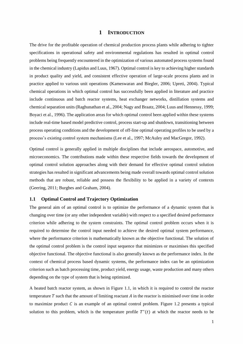
A heated batch reactor system, as shown in Figure 1.1, in which it is required to control the reactor

temperature 𝑇 such that the amount of limiting reactant 𝐴 in the reactor is minimised over time in order

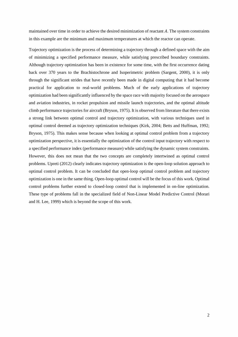
to maximize product 𝐶 is an example of an optimal control problem. Figure 1.2 presents a typical

solution to this problem, which is the temperature profile 𝑇∗(𝑡) at which the reactor needs to be

2

maintained over time in order to achieve the desired minimization of reactant 𝐴. The system constraints

in this example are the minimum and maximum temperatures at which the reactor can operate.

Trajectory optimization is the process of determining a trajectory through a defined space with the aim

of minimizing a specified performance measure, while satisfying prescribed boundary constraints.

Although trajectory optimization has been in existence for some time, with the first occurrence dating

back over 370 years to the Brachistochrone and Isoperimetric problem (Sargent, 2000), it is only

through the significant strides that have recently been made in digital computing that it had become

practical for application to real-world problems. Much of the early applications of trajectory

optimization had been significantly influenced by the space race with majority focused on the aerospace

and aviation industries, in rocket propulsion and missile launch trajectories, and the optimal altitude

climb performance trajectories for aircraft (Bryson, 1975). It is observed from literature that there exists

a strong link between optimal control and trajectory optimization, with various techniques used in

optimal control deemed as trajectory optimization techniques (Kirk, 2004; Betts and Huffman, 1992;

Bryson, 1975). This makes sense because when looking at optimal control problem from a trajectory

optimization perspective, it is essentially the optimization of the control input trajectory with respect to

a specified performance index (performance measure) while satisfying the dynamic system constraints.

However, this does not mean that the two concepts are completely intertwined as optimal control

problems. Upreti (2012) clearly indicates trajectory optimization is the open-loop solution approach to

optimal control problem. It can be concluded that open-loop optimal control problem and trajectory

optimization is one in the same thing. Open-loop optimal control will be the focus of this work. Optimal

control problems further extend to closed-loop control that is implemented in on-line optimization.

These type of problems fall in the specialized field of Non-Linear Model Predictive Control (Morari

and H. Lee, 1999) which is beyond the scope of this work.

3

Figure 1.1: A heated batch reactor system where the reactor temperature is controlled over time

Figure 1.2: Optimal control temperature profile for a heated reactor system

𝐴 + 𝐵 → 𝐶

𝑇(𝑡)

𝑇∗(𝑡)

𝑇𝑖𝑚𝑒 (𝑡)

𝑇 (

𝐾)

𝑇𝑚𝑎𝑥

𝑇𝑚𝑖𝑛

4

1.2 Techniques for solving optimal control problems and their limitations

Optimal control problems are solved through a model based approach where the dynamic system

behaviour is modelled by Differential-Algebraic Equations (DAEs) that are utilised to solve the

optimization problem of determining control input trajectory functions that minimize/maximize a

specified performance index. When applied to chemical process systems, the DAEs consist of Ordinary

Differential Equations (ODEs) for material and energy balances, and equations describing relevant

physical and thermodynamic relations. Ideally, the aim of solving the optimal control problem is to

obtain the optimal controls expressed as explicit functions of the system state (temperature, pressure,

flowrate etc.). It is possible to obtain these functions for linear systems through analytical methods that

are based on the calculus of variations, however they are very difficult to achieve for non-linear systems

that possess constraints as inherent in majority of process engineering applications (Dadebo and

Mcauley, 1995; Bequette, 1991). Numerical techniques present a suitable alternative to the analytical

approach as they effectively allow for the optimal control of more complex nonlinear systems to be

solved for, however these are Initial Value Problem based and need the initial system conditions to be

specified. As a result, the solution obtained is limited in application to this specified initial system state.

If the system initial state changes, a new optimal control will need to be solved for numerically (Upreti,

2012). This is due to optimal control trajectories of the numerical solution not being a function of the

system state any more, unlike the analytical case. These are often called open-loop controls because

when applied, they do not account for the disturbances that may occur to the system.

Significant advancements have been made in the theory and the mathematical development of

numerical methods for solving optimal control problems but the available solution strategies still

possess limitations. These limitations include:

• The solutions obtained not guaranteed as globally optimal

• The applicability of approaches being dependent on the nature and characteristics of the

systems to which they are implemented

• The inability to successfully determine a solution for systems that are highly non-linear and

that possess inherent characteristics such as discontinuities and constraints in the DAEs that

describe the system

• The computational power and computation time required to determine a solution being

unrealistic for real-world problem implementation.

A classification of the currently developed optimal control solution strategies are presented in Figure

1.3. These are broken down to indirect, direct, enumeration and search based methods.

5

Figure 1.3: Optimal control solution strategies

The indirect method, also known as the variational approach, is one of the earliest developed approaches

for solving the optimal control problem. It is based on the first order conditions necessary for optimality

obtained from the calculus of variations which results in a Two-Point Boundary Value Problem

(TPBVP) that is usually solved by mathematical methods that include single shooting, invariant

embedding, multiple shooting or the collocation of finite elements. The variational approach has been

extensively applied to chemical process engineering based optimal control problems, however it can

only be effectively applied to simple systems that are continuous and fully differentiable. Problems of

this nature are not frequently encountered in the dynamic modelling of chemical processes (Lee et al.,

1999). Problems that contain inequality constraints are also difficult to solve using the variational

approach as these require the selection of suitable guesses for the state and adjoint variables of the

resulting TPBVP, making the TPBVP much more difficult to solve (Sargent, 2000).

In the direct method, the optimal control problem is transformed into a finite dimensional Non-Linear

Programming (NLP) problem that is then solved by applying developed state-of-the art NLP solvers.

These methods are divided into sequential, simultaneous and multiple shooting strategies. The

sequential approach involves the discretization of the system control variables and further representing

them as piecewise polynomials, with the optimal control being determined by optimizing the

coefficients of these polynomials. Sequential solution strategies are relatively simple to construct and

apply as they contain the components of existing reliable DAE and NLP solvers (eg. DASSL, SASOLV,

DAEPACK, NPSOL, SNOPT). Their structure however requires the iterative execution of intensive

optimization processes that result in a significant amount of computations being required to determine

a solution. The sequential approach is also well known to be very limited in application to unstable

systems (Biegler et al., 2002; Ascher and Petzold, 1998).

These limitations are overcome by applying the simultaneous approach where both the state and control

variables are discretized across the time domain through the collocation of finite elements. This

Optimal

Control

Indirect

(variational) Direct (NLP)

Enumeration Evolutionary

Search

• Analytical

• Numerical

(Single shooting,

multiple

shooting,

collocation)

• Sequential

• Simultaneous

• Multiple

Shooting

• Dynamic

Programming

• Iterative

Dynamic

Programming

(IDP)

• Genetic

Algorithms

• Evolutionary

Algorithms

6

approach allows for more accurate solutions to be obtained even for unstable systems while being less

computationally intensive. Coupling the model of the DAE system with the optimization problem

results in the DAE being solved for once, at the optimal point. This avoids the evaluation of intermediate

solutions that my not exist or may require excess computational effort. The state and control variable

discretization and DAE Model/Optimization problem coupling however results in very large-scale NLP

problems that require specialized Sequential Quadratic Programming (SQP) based optimization

strategies to be solved. The application of these strategies is more suited for problems in which the

number of control variables are significantly larger than the number of state variables, which is often

not the case in many dynamic processes, particularly in the context of chemical processes (Betts and

Frank, 1994; Betts and Huffman, 1992).

The multiple shooting method is termed to lie in between the sequential and simultaneous approaches,

possessing some advantages from both these methods. In addition to the control variable

parameterization like in the sequential approach, the time domain for the system is discretized into finite

time elements. This allows the DAE to be integrated separately in each element thus eliminating the

requirement for repeated evaluation of the DAE over the entire time domain when optimizing the

control variable polynomial parameters like in the case of the sequential approach. This results in

reduced computation time even for large scale problems, however this approach is unsuccessful in

providing a solution for problems with inequality constraints that lie between the grid points that are a

result of the time domain discretization (Bock and Plitt, 1984). Overall, due to the nonlinear, multimodal

and discontinuous nature of chemical process engineering systems, indirect methods are frequently

known to provide the locally optimum result dynamic optimization problems.

Dynamic Programming is a popular enumeration based optimization approach that is based on the

Bellman principle for optimality, where the optimization problem is solved by breaking it down into

local sub-problems (Bellman, 1954). This approach guarantees the calculation of the global optimal

control solution when neglecting approximation errors that are a result of the modelling and

discretization of the system state space (van Berkel et al., 2015). The numerical framework of Dynamic

Programming allows for effective implementation for systems that have non-linear dynamics and

possess non-continuous constraints. The application of Dynamic Programming, however, is limited to

low dimensional problems due to exponential increase in computation time as the dimensions of the

dynamic systems increases (Bertsekas, 2007).

Evolutionary search algorithms on the other hand are stochastic based optimization methods that mimic

mechanisms found in natural genetics such as reproduction, mutation and genetic crossing over

(Goldberg, 1989). This class of algorithms are further subdivided into Genetic Algorithms (GA) and

Evolutionary Algorithms (EA) and follow a two-step process for optimization that includes 1) the

randomly generating a population of points that serve as optimal solution candidates and 2) applying

7

the above-mentioned evolutionary operations to “evolve” these candidates towards an optimal solution

(Michalewicz et al., 1992). This approach offers a higher probability of finding a globally optimal

solution to an optimal control problem as compared to the direct and indirect approaches and is

relatively easy to implement. The global optimum search undertaken by the Genetic and Evolutionary

Algorithms is based on probabilistic transition rules that results in a significantly larger computation

time being required than the direct and indirect method approaches (Lee et al., 1999).

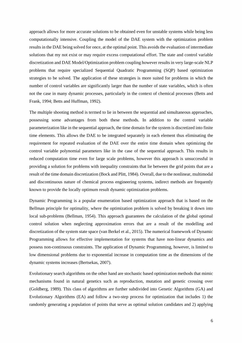
1.3 Graph theory based trajectory optimization

Graphs are simple geometric structures consisting of vertices and edges that connect them. A basic

undirected and directed graph is presented Figure 1.4. This simple diagrammatic representation makes

graphs a very useful for modelling complex systems (Bondy et al., 1976). It is fair to say that graph

theory, the field behind the development, representation, characterization and analysis of graphs is well

established; with extensive work being done since the introduction of the concept in the 17th century

through Leonhard Euler’s (1736) work on the Königsberg Bridges Problem (Gross and Yellen, 2004).

Just like trajectory optimization, the application of graph theoretic solution approaches to practical

problems has only been recently adopted through the advent of the digital computer. This has seen graph

theory being actively applied in chemistry (modelling of molecular structures), engineering, computer

science (algorithm development), economics, operations research (scheduling) and many others

(Dharwadker and Pirzada, 2007; Bales and Johnson, 2006; Mackaness and Beard, 1993).

Figure 1.4: Graphical representation of vertices and edges in an undirected (left) and directed (right)

graph

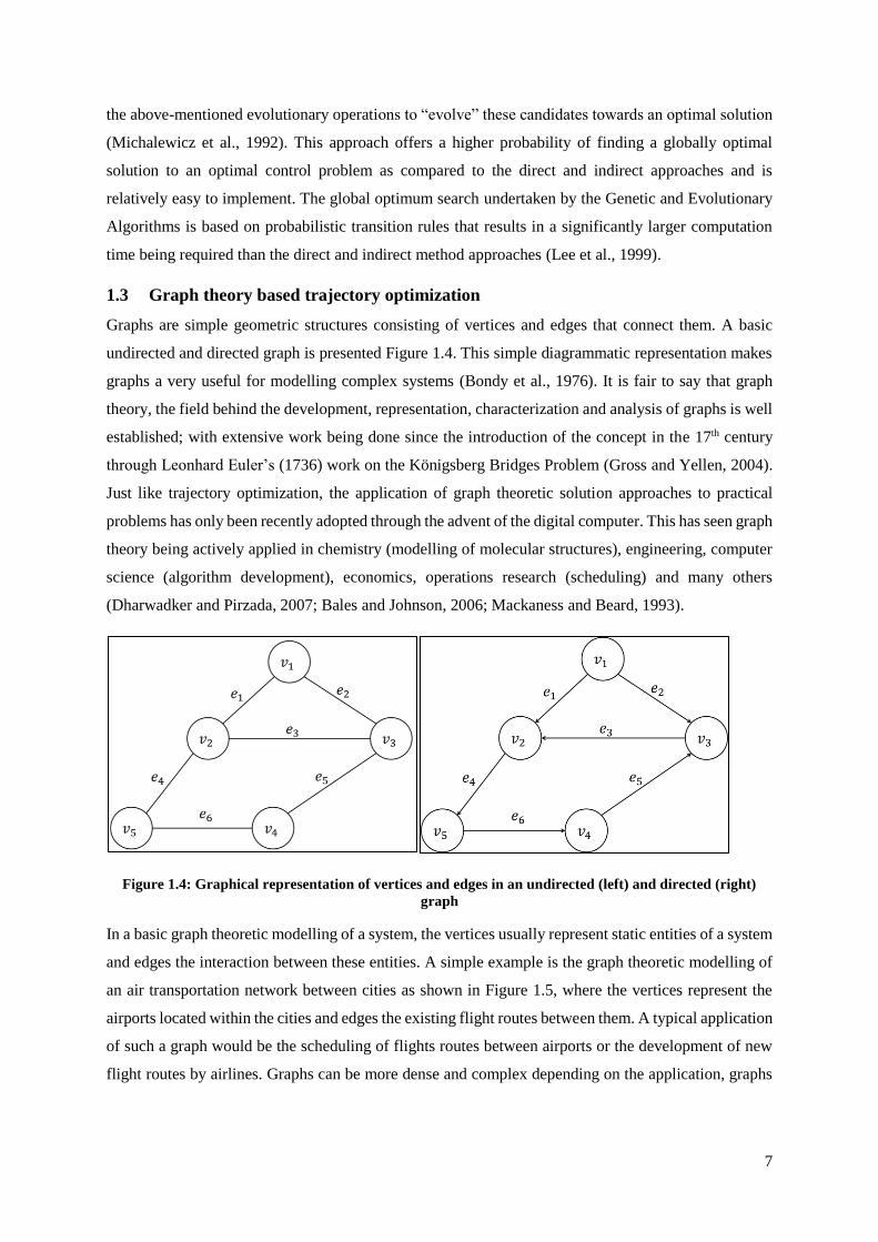
In a basic graph theoretic modelling of a system, the vertices usually represent static entities of a system

and edges the interaction between these entities. A simple example is the graph theoretic modelling of

an air transportation network between cities as shown in Figure 1.5, where the vertices represent the

airports located within the cities and edges the existing flight routes between them. A typical application

of such a graph would be the scheduling of flights routes between airports or the development of new

flight routes by airlines. Graphs can be more dense and complex depending on the application, graphs

8

can be more complex as in the modelling of large-scale systems such as communication and

transportation networks (Bhattacharya and Başar, 2010; Bales and Johnson, 2006).

Graph theoretical concepts have been extensively applied in solving trajectory optimization problems

that appear in a wide variety of contexts. Some examples of such problems include the travelling

salesman problem, the shortest spanning tree problem and locating the shortest path between two points,

with these successfully applied in operations research, navigation systems and game theory, where

systems are modelled as graphs (Shirinivas et al., 2010). Mathematics and computer science have

contributed significantly over the recent years to the numerous algorithms available for solving graph

theoretic based trajectory optimization problems. However, unlike the trajectory optimization

techniques described above, these algorithms are not intended for continuous systems and are limited

to discrete systems where the graph elements represent defined static entities. Graph theoretic

approaches have previously been applied in modelling linear control systems but are mainly intended

for graphical analysis and deriving system structural properties such as controllability, observability,

solvability and symbolical analysis (Boukhobza et al., 2006; Reinschke and Wiedemann, 1997;

Reinschke, 1994). There still remains a gap in the graph theoretical modelling of non-linear systems.

Figure 1.5: Map showing graph theoretic representation of air networks between airports in India

(obtained from www. mapsofindia.com Accessed 13/08/2016)

9

1.4 Shortest path graph algorithms

The shortest path graph search problem can be observed as a discrete trajectory optimization problem.

Depending on the application, the problem may require the computation of the shortest paths from a

source vertex to every other vertex (one-to-all) or from every vertex to every other vertex (all-to-all) in

a graph. In some instances, it can only be necessary to compute shortest paths from a source vertex to

a single destination vertex (one-to-one). Numerous real-world routing problems are modelled such that

the vertices are associated with a particular state, process or location and the edges linking these to

contain a cost (representing distance, weight, time or any desired quantified metric) for travelling across

each edge. Determining the shortest paths in such a context can provide the best route for navigating

from one point to another in the system. One common instance of this is in Global Positioning System

(GPS) based route navigation where weighted directed graph models represent road networks with

vertices representing intersections and the edges the roads between them, with edge weights

representing their respective total road distances. Implementing a shortest path graph search algorithm

to determine the distance between a specific start and end city essentially determines the minimum

cumulative cost in distance between these two points.

Graph theoretic computation of shortest paths is well known to be a computationally intensive task,

particularly for problems that involve dense graphs with a large number of vertices and edges as often

seen when solving problems relating transportation and network analysis (Zhan and Noon, 2000). As a

result, majority of algorithm development for solving these problems is geared towards high

performance algorithms that obtain optimal shortest path solutions while reducing computation time.

This is necessary to allow for problem solving and analysis in graphs that contain hundreds of thousands

or even millions of vertices as frequently encountered in the modelling of real world systems.

The most common shortest path graph search algorithms apply a graph labelling procedure where

vertices in the graph network are labelled and updated during the search for the shortest path from a

specified source (Gillian, 1997). Graph labelling methods are categorized into two groups: label-setting

and label-correcting. Both these methods follow an iterative procedure in the labelling of the vertices,

however they differ in the manner at which shortest path distances associated with each vertex are

updated at each iteration. Theoretically, label-correcting and label-setting methods are both expected to

perform equivalently in computing the one-to-all and all-to-all shortest paths, however the label-setting

approach is expected to be more efficient for computing the one-to-one shortest path (Zhan and Noon,

2000). It cannot be concluded on which approach universally outperforms the other as the effectiveness

in computation is dependent on various other factors that include the structure of the graph network to

which the algorithm is being implemented and the data structure used for storing and labelling the

vertices when the search is conducted.

10

This work focuses on the application of Dijkstra’s Algorithm (Dijkstra, 1959), a label-setting based

algorithm that guarantees the optimal solution for the shortest paths for the one-to-all shortest path

problem. It also relatively easy to extended for implementation to the ono-to-one and all-to-all based

problems (Cormen et al., 2009).

1.5 Closing Remarks

In practice, shortest graph search algorithms are a powerful tool for trajectory optimization of graph

theoretically modelled discrete systems. These algorithms in combination with the elegant

representation of entities and relationships that can be achieved through graph theoretic modelling along

with the continued increase in computational processing power present a promising opportunity for the

successful development of graph theoretic search approach for determining the optimal control of

chemical process systems modelled by DAEs. Graph theoretic approaches for optimization of DAEs

based systems have not yet been widely adopted in practice. This is largely due to a multitude of tools

and packages that have already been developed, particularly for NLP based approaches. These are state

of the art and generally require in depth knowledge of NLP approaches for effective application, which

can be a limiting factor for certain applications.

Successfully developing a shortest path graph search based approach for solving optimal control

problems however will require effective graph theoretical modelling of the dynamic system. The graph

theoretic model must also be such that it contains all the elements of the optimal control problem.

Therefore, the major focus of this work involves applying graph theoretical modelling principles to

effectively translate the optimal control problem for a dynamic system governed by DAEs into a shortest

graph search problem such that the solution obtained is an optimal control input trajectory that can

directly be applied to the system.

11

2 LITERATURE REVIEW

2.1 Graph theoretical modelling of discrete systems

Graphs provide a robust simplistic framework for modelling the relations and dynamics that exist in

natural and man-made systems. This has resulted in graph theoretic modelling being applied to many

practical problems across a wide diversity of fields. The expansive growth of graph theoretical

modelling over the past few decades due to the continued increase in computational processing ability,

better availability of data and interdisciplinary collaborations has made it realistically possible to model

and solve problems for more complex real-world systems that possess thousands or even up to millions

of interactions between their respective elements.

2.1.1 Early Developments

2.1.1.1 Traversability

The first instance of graph theoretical modelling is traced back to Euler’s work on the Seven Bridges

of Konigsberg problem that aimed to determine a path through the city of Konigsberg that crossed each

of the seven bridges that connected two large islands with two mainland parts of the city only once.

Attempting to solve this problem subsequently led to Euler producing a paper on “The solution of a

problem relating to geometry of position” (1736) where he theoretically proved that the problem had

no solution. Euler did not explicitly use graph theoretical modelling when he attempted to solve the

problem but reformulated it to a problem of finding a sequence of eight letters representing the path

across the bridges where the number of times the letter pairs representing regions connected by the

bridges were adjacent, corresponded with the number of bridges connecting the regions. Thus in his

work, he proved that no such sequence exists, hence proving the non-existence of a solution for the

problem. The first usage of graph theory for solving this problem is attributed to Rouse Ball (1892) who

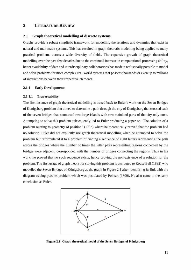
modelled the Seven Bridges of Königsberg as the graph in Figure 2.1 after identifying its link with the

diagram-tracing puzzles problem which was postulated by Poinsot (1809). He also came to the same

conclusion as Euler.

Figure 2.1: Graph theoretical model of the Seven Bridges of Königsberg

12

2.1.1.2 Chemical Trees

A tree is defined as a connected graph without cycles and first appeared in Kirchhoff’s work in the

application of graph theoretical ideas in determining currents in electrical networks (1824-1827). Over

a century after Euler’s work on the bridges of Königsberg problem Sylvester (1878), Cayley (1879,

1874), PòPolya (1987) and a few others (Read, 1963; Harary, 1955; Otter, 1948) contributed to

significant developments in applying trees to solve problems that involved enumeration of chemical

molecules.

The graph theoretic representation of chemical molecules first occurred in the graphic formulae

representation of molecules which led to the explanation of isomerism. Cayley (1874) later applied tree-

counting methods to enumerated isomers for alkanes of up to 11 carbon atoms and other molecules.

Little progress however was made in the numeration of isomers until the 1930’s through PòPolya’s

work that applied permutation based principles for solving the isomer-counting problem for several

families of molecules.

2.1.1.3 The Four-Colour Problem

The four-color problem can be attributed to many developments in graph theoretical modelling. Its first

mention dates back to 1952 when Francis Guthrie tried to determine whether it is possible for every

map to be coloured with just four colours such that no countries that share the same border have the

same colour. Kempe (1879) presented the first solution to the problem resulting in a proof called the

four-color theorem where he showed that every map had to contain a country with at most 5 neighbours

in order for a map to be coloured with four colours such that no countries with the same colour share a

border. Heawood (1949) later proved that Kempe’s theorem was incorrect, further deducing the five-

colour theorem and extending the problem to other surfaces. Birkhoff’s (1912) major contribution in

the investigation of the number of ways in which a map can be coloured for an arbitrary number of

colours led to Franklin (1922) deducing the four-colour theorem to be true for maps with up to 25

regions. Appel and Haken (1989) eventually confirmed the four-colour theorem by providing a

computer-assisted proof resulting in the four-colour theorem being the first major theorem to be proved

with the aid of a computer. The graph colouring techniques developed for proving these theorems have

found more modern applications that include time table scheduling, computer network security and the

assignment of frequencies in Global System for Mobile Communications (GSM) mobile phone

networks (Chachra et al., 1979).

2.1.2 Common Engineering Applications

In electrical systems analysis, graph theoretical modelling has been successfully applied in the analysis

of interactions between resistors, voltage supplies, capacitors and other elements that may exist in

electrical networks by modelling these as a directed graph. One of the earliest implementations of graph

theory in electrical systems analysis can be traced back to the work of Kirchoff (1845) where he

13

developed rules that govern the flow of current in a network of wires. These include the deductions that

the algebraic sum of the current flowing through the network junction and the sum of the potential

difference around a closed circuit in the network both being equal to zero. These rules formed the basis

for the deduction that it isn’t necessary for an exhaustive examination of an entire circuit in order to

determine the current for all its constituent wires, which lead to the development of a method for

identifying the set of fundamental circuits necessary for the current of all wires in a circuit. These

methods are still used today. Further detailed review for applications of graph theory in electrical

engineering systems can be found in Stagg and El-Abiad (1968), Swamy and Thulsiraman (1981), and

Berdewad and Deo (2014).

Graph theoretic models are extensively utilized in the industrial engineering field, most commonly in

project planning through the mapping of precedence relationships between activities and events

required for the completion of a project (Foulds, 2012). The two common modelling approaches include

the activity-oriented and event-oriented directed graphs, which differ in the manner at which the

precedence relationships are abstracted into graph theoretical elements, where vertices are used to

represent activities and events for the activity-oriented and event-oriented methods respectively. The

event-oriented approach however is rather more popular compared to the activity-oriented approach as

the activities that result in the vertex modelled events are modelled as the edges with their respective

durations further modelled as edge weights, as a result providing the advantage of planning solutions

being more effectively solved for by computer (Robinson and Foulds, 1980). The application of graph

theoretic approaches for the Critical Path Method (CPM) and Program Evaluation and Review

Technique (PERT) project scheduling methods is presented in further detail by Hindelang and Muth

(979) and Robinson and Folds (1980). Beyond project activity scheduling, directed graphs have also

been useful in resource allocation and optimization problems that arise in the industrial engineering

context, with the most common problem being that which requires the minimization of workstations

required to complete tasks that are to be distributed across them without violating any existing

constraints (Gross and Yellen, 2004).

2.2 Fundamental graph search algorithms

Solving problems for practical systems that are modelled as graphs often requires the analysis of the

underlying graph model and evaluating it for desired properties. Graphs that arise from the modelling

of practical problems are usually large and complex. This makes it relatively important that algorithms

developed for achieving the desired analysis are efficient, suitable for implementation on a digital

computer and provide the necessary results within a time frame that is feasible enough to implement

them. The characteristics for measuring algorithm performance are its completeness, optimality,

computational time complexity and computational space complexity. The completeness of an algorithm

is a measure of whether it is guaranteed to determine a solution to the problem if it exists, while an

algorithm’s optimality is an indicator of whether it is able to determine an optimal solution. The

14

computational time and space complexity is the measure of the number of elementary instructions

(executed by the algorithm during its runtime) and the working memory required for the algorithm to

determine a solution respectively. The time complexity of an algorithm is specified using the O-notation

eg, 𝑂(𝑛). The measurement of algorithm time complexity using O-notation is described in extensive

detail by Cormen et al. (2009). Ideally, an effective algorithm is complete and is able to obtain the

optimal solution at the least possible computational time and space complexity. This generally is not

the case for many of the algorithms dedicated towards complex graph theory based problems.

Graph search algorithms are a set of algorithms that usually aim to find a certain vertex within a graph

that represents a certain property of the graph theoretically modelled system and are generally used to

solve theoretical and practical Discrete Optimization Problems (DOP) related to graphs representing

discrete systems. Some common examples of these include the motion planning of robots, systems

control and logistics (Kumar et al., 1994). The two main fundamental algorithms for graph theoretic

search are Breadth-first Search (BFS) and Depth-first Search (DFS), first published by Moore (1959)

and Tarjan (1976) respectively with later developed graph search algorithms usually being the result of

a modification of these to improve their computational efficiency, the optimality of solution or suit a

particular application.

2.2.1 Breadth-first Search

The Breadth-first Search algorithm is an uninformed graph search strategy that systematically traverses

a graph by evaluating all the neighbours of a given vertex first before proceeding to the neighbours of

its neighbours. Eventually every vertex that is reachable from a specified source vertex is discovered,

resulting in a breadth-first tree containing all the reachable vertices with source vertex as the root

(Cormen et al., 2009). BFS was first discovered by Moore (1959) in finding paths through mazes and

also independently discovered by Lee (1961) in routing wires on electrical circuit boards. The main

usage of the BFS algorithm is in determining the shortest path (in terms smallest number of edges) from

a specified source vertex to every other reachable vertex in the graph and is known for the simplicity it

provides in determining this solution in various applications (Kadhim et al., 2016). BFS is complete,

however the paths to the target vertices are only optimal for graphs were all the edges connecting the

vertices are have no edge costs and in graphs where the edge costs are a non-decreasing function of the

target vertices’ depth from the source vertex. In its implementation, BFS requires the storage of every

vertex that is reached in the search, making it significantly memory intensive relative to other graph

search algorithms. This results in space complexity being the major constraint in its applicability to

large an complex graphs (Russell and Norvig 2002).

Breadth-first Search was initially intended to solve maze-based problems for determining the shortest

path from an entry point to an exit point in a maze. However over the years, BFS has also been utilized

for solving several other problems that include determining the shortest path between two nodes, the

15

serialization and deserialization of data and the computation of maximum flow in a flow network

through the Ford-Fulkerson method (Kadhim et al., 2016).

The progressive advancements made in computational processing and memory handling methods,

particularly in parallel processing and distributed memory architecture, have resulted in significant

work being done in order to improve effectiveness of the BFS algorithm in solving problems for large

and dense graphs. The most recent developments in this domain include notable work in Graphical

Process Unit (GPU) based BFS parallelization that includes the Nvidia GPU and CUBA based

implementation of BFS by Harish and Narayanan (2007), and the GpSM GPU massive architecture

method used for sub-graph matching introduced by Tran et al. (2015). These approaches accelerate the

Depth-first search process by taking advantage of the strong parallel processing ability of current GPUs.

Distributed memory architecture based techniques have also been employed to overcome the scalability

problems that come with the parallel processing of BFS in large graphs. The most significant

contributions in this domain are the fast Partitioned Global Address Space (PGAS) parallel

programming model for graph algorithms that Cong et al. (2010) developed by improving the memory

access locality and the efficient versions of BFS proposed by Checconi et al. (2012) on the IBM Blue

Gene/P and Blue Gene/O supercomputer architectures. High performance in terms of computational

runtime was achieved on a massively large and dense graph by employing various distributed memory

techniques that include bitmap storage, removal of redundant predecessor map updates, compression

and more efficient representation of the graph elements. Parallelized BFS algorithms have been

successfully applied in algorithms for planarity testing, determining of minimum spanning trees and

assessing graph connectivity (Savage and Ja’Ja’ 1981; Ja’Ja’ and Simon 1982). Implementing these by

utilizing supercomputer architectures makes the application of these BFS based algorithms to graphs

that model complex “big data” applications such as social network analysis, biological systems and data

mining (Lu et al., 2014).

2.2.2 Depth-first Search

The first occurrence of the Depth-first Search strategy was in investigations performed by Lucas (1882)

and Tarry (1895) in the exploration of a maze, with the fundamental properties of DFS only being later

developed and defined by Hopcroft and Tarjan (1973, 1974) in their work on DFS and Depth-first Trees.

The idea behind the DFS strategy is that it explores the graph by repeatedly selecting the first incident

edge of the most recently reached vertex, thus going deeper in the graph until a vertex that does not

have any further unvisited neighbouring vertices to be explored is reached. Upon reaching this ”dead

end” vertex, the search then undertakes a backtracking procedure where it returns to the most recently

reached vertex whose neighbouring vertices have not yet been explored and continues to perform the

Depth-first search (Cormen et al., 2009; Gross and Yellen, 2004; Tarjan, 1976). This process continues

until all vertices reachable from a specified source vertex are reached, resulting in a depth-first tree.

16

DFS has been widely recognized as a powerful technique for solving various graph problems and has

been generally used in algorithms for identifying spanning trees (Reif, 1985; Tarjan, 1976),

isomorphism (Ullmann, 1976) and fundamental cycles in graphs (Bongiovanni and Petreschi, 1989).

DFS is also extensively used in Artificial Intelligence for solving problems in decision making, planning

and in expert systems (Russell and Norvig, 2002). The success of DFS however in determining a

solution is highly dependent on the structure of the graph as it is susceptible to non-termination issues,

particularly the exploration of infinite loops that result in certain vertices in the graph not being reached

and a solution not being determined. A vertex checking modification is usually used to avoid the infinite

loops problem, however the Depth-first exploration of the redundant paths that result in infinite loops

prior to detection, particularly in exceptionally large sized graphs, still remains an issue (Russell and

Norvig, 2002). DFS is complete when implemented such that it avoids repeated states and redundant

paths when applied to a finite graph as this results in every vertex from a specified source vertex will

be reached (Cormen et al., 2009). DFS however has no distinct advantage over BFS in terms of time

complexity and optimality when applied to a finite graph. This is due to the time complexity of DFS

being determined by the number of vertices and edges of the graph. The DFS approach however can be

highly computationally inefficient when applied to the unique graph search problem that requires the

determination of a path from a specified source vertex to a specified destination vertex in the graph.

This is because the search might traverse the entire graph in one DFS path, only to find that it doesn’t

lead to the desired path before backtracking and searching other DFS paths. This issue was resolved by

the development of the Iterative Deepening Depth-first Search (IDDFS) by Korf (1985), an approach

that is a combination of the BFS and DFS that utilizes the optimality of BFS and the space complexity

efficiency of DFS.

DFS can be applied using parallel programming techniques. Parallelized DFS was first developed by

Rao and Kumar (1987a, 1987b) and further implemented in directed graphs by (Aggarwal et al., 1989).

DFS is highly sequential search approach (Korf, 1985) and the application of parallel implementations

can only provide significant improvements in computational performance through the exploitation of

structure of the graph that has to be known prior to implementation (Freeman, 1991).

2.3 Shortest path graph search

Efficient route planning is essential and plays a significant role in research, business and many

industries. Typical examples where route planning has proved to be critical in industry include network

cabling, the design and operation of electricity and water supply networks, and the scheduling of

projects (Sadavare and Kulkarni, 2012). Determining shortest paths plays a significant role in

optimization within these systems, with the most common type being the one-to-one shortest path

problem that requires a path from a specified starting point to a desired destination that results in the

least cumulative cost. Advances made in graph theoretical modelling and developments in graph search

algorithms have made the graph theoretic approach more viable in fulfilling the need for procedures

17

that are more efficient in providing solutions to these problems in order to achieve better optimized

operation of these systems. This has resulted resulting in shortest path graph search algorithms being

among a small group of efficient algorithms dedicated to handling this class of problems.

2.3.1 Shortest path graph algorithm methods

Mathematical research into the shortest path problem is observed to have started relatively late when

compared to graph theory based combination problems like the minimum spanning tree. Path

optimization problems only became a major interest in the early 1950’s and were studied for solving

alternate routing problems encountered in freeway usage by Trueblood (1952). His approaches were

based on the classical work of Wiener (1873), Lucas (1882) and Tarry (1895) on graph theoretic

approaches for search through a maze. The approaches developed in this time were divided into matrix

based methods, linear programming and enumeration.

2.3.1.1 Matrix manipulation methods

Matrix manipulation based methods were developed and applied in studying relations between entities

in networks. An example is determining a relation between two entities in a graph theoretic

representation of a network by determining whether they are reachable from each other. This was

achieved by representing a directed graph model of the system/network as a matrix and performing

iterative matrix products to determine the existence of a path between two specified points/entities.

Notable work in this area includes studies conducted by Luce (1950), Lunts (1952) and Shimbel (1951,

1953, 1954).

Shimbel (1951, 1953, 1954) whose interest in matrix methods was motivated by their application in

communication between neural nets, extended the matrix methods he had developed to determine unit

length paths. His approach (Shimbel, 1954) is observed to be similar to the Bellman-Ford algorithm but

observed to possess a much larger computational time complexity of 𝑂(𝑛4) in determining the distances

between all pairs of vertices in a graph. Even though matrix based approaches present a promising

approach for determining shortest paths, they still possess attributes that made them unsuitable for many

applications. These included the matrix products being computationally intensive which makes them

impractical for application to large systems and their limitation in only being able to determine shortest

paths for graphs of unit length edge weights. An improvement on the computational complexity of

Shimbel’s method was made by Leyzorek et al. (1957) of the Case Institute of Technology resulting in

the all pairs shortest path problem being solved in a time of 𝑂(𝑛3 log 𝑛). This improvement can only

be observed when applied to graphs with a large number of vertices and edges, still making the matrix

approach highly impractical.

2.3.1.2 Linear programming based method

Orden (1956) observed that the shortest path problem can be solved through linear programming by

showing that it is a special case of a transhipment problem. A procedure for applying the simplex

18

method to solving this problem was later presented by Dantzig (1957) where he illustrated its validity

by solving the problem of transporting a package between cities in a real-world road network. A similar

approach was presented also proposed by Bock and Cameron (1958), however it was later shown by

Edmonds (1970) that simplex based approaches to the shortest path problem take exponential

computation time (computations required increases exponential with number of points/vertices),

proving them to be highly impractical for many real-world applications.

2.3.1.3 Enumeration based methods

The first instance of the application of enumeration based search in the solving of the shortest path

problem is in Ford's (1956) method for finding the shortest path from a specified source vertex 𝑣0 to

destination vertex 𝑣𝑁 in a graph containing vertices 𝑣0 … 𝑣𝑁. Ford’s method achieved this by first

assigning the distances of all vertices in the directed graph from the specified initial vertex to infinity

and then scanning all the graph vertices and updating the distances to the destination vertices. The

distances were updated by locally comparing the distances of respective neighbouring vertices from the

source vertex 𝑣0 and updating them if their difference was greater than the weight of the edge

connecting them. This approach has been proven to be complete, however it was shown by Johnson

(1973) that it takes exponential time, making it impractical for determining shortest paths dense graphs

(graphs with a significantly large of number of edges).

After successfully developing and publishing several papers on Dynamic Programming, Bellman

(1958) developed a functional equation approach that turned out to be similar to that which was

presented by Shimbel (1954). As opposed to Shimbel's (1951) matrix manipulation approach, Bellman's

(1958) approach was enumerative and iterative, possessing a computational time complexity of 𝑂(𝑉3)

where 𝑉 was the number of vertices. Accounting for the time complexity, Bellman (1958)

recommended his approach to be feasible for graphs that contained 50-100 vertices (V=50-100).

Dantzig (1960) presented an algorithm for evaluating the shortest path between a source and a target

vertex in graphs with non-negative edge weights with a computation time of 𝑂(𝑉2 log 𝑉), an

improvement in computation time from Bellman's (1958) approach. Dijkstra's (1959) presented

Dijkstra’s Algorithm which, like Dantzig's (1960) algorithm, determined the shortest path from a source

vertex to every other vertex in a non-negative weighted graph. Dijkstra’s Algorithm however was much

easier to implement and had a much reduced computational complexity of 𝑂(𝑉2) however much

reduced computational time complexities were later achieved through more efficient data structures.

2.3.2 Shortest Path Algorithms used in current practice

The current well known well known and frequently used shortest path graph search algorithms in

practice include Dijkstra’s Algorithm (Dijkstra, 1959), the Floyd-Warshall Algorithm (Floyd, 1962)

and the Bellman-Ford Algorithm (Ford, 1956; Bellman, 1958; E. F. Moore, 1959). These are a result of

19

a combination of elements from original that was work done in the development methods for solving

the single-source and all-pairs shortest path problems.

2.3.2.1 Dijkstra’s Algorithm

Dijkstra’s Algorithm is graph one of the most robust shortest path graph search algorithms in practice

for the single source shortest path problem. Current implementations still remain largely similar to that

which was presented by Dijkstra (1959), however over the past few decades, improvements have been

made in the computation time complexity of the original algorithm through the utilization of more

efficient data structures for scanning and storage of vertices contained in the graph state space. The

most commonly used data structures for implementing Dijkstra’s Algorithm are the Binary Heap that

was developed by Vuillemin (1978) and the Fibonacci Heap which was introduced by Fredman and

Tarjan (1987). The binary heap data structure is generally more preferred due to its ease of

implementation. The binary heap and Fibonacci heap are observed to result in an improved computation

complexity of 𝑂(𝐸 log 𝑉) and 𝑂(𝐸 + 𝑉 log 𝑉) respectively as compared to the 𝑂(𝑉2) of the original

algorithm. Theoretically, the Fibonacci heap is meant to result in a much improved algorithm runtime

however the difference in performance can only be observed in significantly dense graphs (Goldberg

and Tarjan,1996). More efficient implementations of Dijkstra’s algorithm were further studied and

developed, the most notable being an algorithm presented by Ahuja et al. (1990) through the

development and implementation of the Redistributive Heap data structure, and the algorithm by

Thorup (2004) that achieved a runtime of 𝑂(𝐸 + 𝑉 log(log 𝑉)) using Fibonacci heap based integer

priority queues.

2.3.2.2 Bellman- Ford Algorithm

The Bellman-Ford algorithm is a single source shortest path algorithm that was first introduced by

Lawler (1976) and is a result of previous work by Ford (1956), Bellman (1958) and Moore (1959). A

similar algorithm was presented by Tarjan (1983) however he had not given it a name. Bellman-Ford

has a computational complexity of 𝑂(𝐸𝑉) and is much slower than Dijkstra’s algorithm in determining

shortest paths. This is due to Bellman-Ford algorithm’s iterative structure that iterates through a graph

with 𝑉 vertices 𝑉 amount of times while processing all of the edges in the graph in order to update the

distances of all the graph vertices from the source vertex with each iteration (Cormen et al., 2009). The

Bellman-Ford approach provides more versatility compared to Dijkstra’s algorithm because of its

ability to determine the shortest paths in graphs with negative edge weights, making the algorithm very

useful in various applications where systems are modelled with negative and positive edge weights. The

Bellman-Ford algorithm, however, cannot determine the shortest path for graphs that contain negative

cycles but the algorithm can be used to detect them.

Notable improvements that have been made to the Bellman-Ford algorithm in order to improve its

computation time complexity include Yen's (1970) approaches that involved modifying the iterative

20

vertex distance processing and updating procedure. These improvements include skipping the

evaluation of edges for vertices whose distance from the source hadn’t changed from the previous

iteration, partitioning the graph into two directed graphs with no negative cycles and alternating the

iterations for processing the vertex distances between these two graphs. These modifications resulted

the algorithm time complexity being reduced to 𝑂(𝑉3/4). The most recent improvement is by Bannister

and Eppstein (2012) who modified Yen's (1970) approach by random permutation of the graph vertices

and using the resulting the random to process the vertices in each iteration. This results in an improved

computation time of 𝑉3/6 + 𝑂(𝑉3).

2.3.2.3 The Floyd-Warshall Algorithm

The Floyd-Warshall algorithm is an all-pairs shortest path graph search algorithm that determines the

shortest path between every pair of vertices in a weighted directed graph. The algorithm was first

published by Floyd (1962) who based it on Warshall's (1962) theorem for determining the transitive

closure of Boolean matrices. Just like the Bellman-Ford algorithm, Floyd-Warshall is able to determine

the shortest path in graphs that have both negative and positive edge weights but cannot determine

shortest path solutions in graphs that contain negative cycles. It is a much slower algorithm as compared

to Dijkstra’s and the Bellman-Ford algorithm with a time complexity of 𝑂(𝑉3), however several

researchers have presented modifications for improving computation complexity. Fredman (1976) was

able to reduce the computational time complexity to 𝑂(𝑉3(log log 𝑉 / log 𝑉)1/3) by introducing a

vertex pre-processing procedure that reduces the number of comparisons that need to be made between

current and previous all-pair path distances in each iteration. Han (2008) recently provided an algorithm

with a reduced running time of 𝑂(𝑉3(log log 𝑉 / log 𝑉)5/4) through a traditional lookup table technique

that involved the construction of many tables in order to maximise the improvement in computation

time that lookup tables present.

2.4 Shortest path based approaches to optimal control based trajectory optimization

The application of shortest path algorithms as an alternative to solving optimal trajectory problems

based on a specified cost function is a concept that has been recently explored and implemented. The

earliest work presenting this approach was by Tsitsiklis (1995) where he showed that the deterministic

optimal control problem can be solved by applying Dijkstra-like algorithms. In his work, Tsitsiklis

(1995) developed a method for applying serial and parallel shortest path algorithms for solving the

optimal control problem of navigating a car out of a specified region in a defined system state space

while minimising a specified cost functional. This was achieved by discretizing the resulting continuous

Hamilton-Jacobi equation that arises from the system differential equations and cost functional through

finite element discretization such that it can be solved by one-pass algorithms as opposed to traditional

iterative approaches. The developed approach was successful in determining a solution for the optimal

path through a state space with obstacles with the Dijkstra-like algorithm providing the best

21

computation time when compared to the Gauss-Seidel based iterative approach and the Dial-like

parallel shortest path approach. The methods for extracting the optimal control input for the car’s

resulting optimal trajectory through the system state space, however, is not explicitly presented in this

work. Tsitsiklis (1995) also confirmed that the developed shortest path approaches are only applicable

to problems where the cost functional was independent of the control variable, making them limited in

application to many real-world optimal control problems where the cost functional is dependent on the

control. Polymenakos et al. (1998) followed up on this work by developing more computationally

efficient parallel processing based label-correcting algorithms for solving the problem presented by

Tsitsiklis (1995). These algorithms reported to be superior to the Dijkstra-like approach presented by

Tsitsiklis (1995) however further development would be needed to be done for them to be implemented

in systems where the cost functional is explicitly a function of the control input.

Junge and Osinga (2004) formulated a graph theoretic set oriented approach for modelling a

Differential-Algebraic Equation (DAE) based discrete-time non-linear control system as a weighted

directed graph in order to solve the optimal control problem to as a shortest path problem from an initial

state to a desired final state. This approach successfully accommodated cost functionals that were

dependent on the control, with the framework also allowing for the successful retrieval of state and

control input trajectories from the calculated shortest path. It was further reported however that the state

and control trajectory solutions were not the true solution to the problem but were “pseudo-trajectories”

that can be used as a good initial guess for solving the problem via the traditional local optimal control

solution based iterative methods.

Further notable work in the application of Dijkstra’s shortest path algorithm for solving optimal control

problems include the work of Rippel et al. (2005) who developed a method for applying shortest path

algorithms for generating three dimensional optimal flight trajectories. Rippel et al. (2005) achieved

this by approximating the map of the flight region of interest as a finite weighted directed graph through

grid-based discretization making it possible to determine the optimal flight route from the plane’s

departure point to the destination point by utilizing a shortest path algorithm. The edge weights of the

generated graph represented the cost of discrete movements from one point to another on the map and

was based on factors that included time, altitude and riding qualities, which were selected as the criteria

that influences the efficiency of the flight mission. The finite graph of the flight space was generated

from a Digital Terrain Map rather than a differential equation representation of the system. This work

also proposed a few adaptations that could be made to the graph theoretic modelling of the terrain in

order to reduce computation time in order to make the approach feasible for application on-board a

flight. Yershov and LaValle (2011) were also successful in implementing Dijkstra’s algorithm in

determining shortest paths through multi-dimensional spaces containing obstacles. Their approach

however was intended for determining optimal robotic navigation routes without emphasis on

determining the control input policy for generating the resulting navigation paths. These two approaches

22

show that applying shortest path algorithms for solving optimal control problems is possible in practice

however they lacked the ability to accommodate the dynamic aspects of systems described by DAE’s

thus limiting their application to systems modelled by these equations.

2.5 Summary

It can be deduced from this review that shortest path based methods present a viable alternative for

solving the optimal control problem. This is due to their completeness, ability to determine the optimal

solution and more efficient time and space complexities in solving the shortest path search problem.

Previous work presented by Tsitsiklis (1995), Junge and Osinga (2004) have proven that graph

theoretical modelling of non-linear control system dynamics like those frequently observed in chemical

processing is possible. There still remains gap for development of graph theoretic modelling approaches

that allow a complete optimal control solution to be determined from one-pass shortest path algorithms

(like Dijkstra’s algorithm), particularly for systems where the cost functional is a function of the input

trajectory as frequently observed in chemical process based problems.

23

3 THESIS OBJECTIVES

The primary objective of this work was to develop a method for representing a continuum based non-

linear chemical process dynamic control system modelled by Differential Algebraic Equations (DAE’s)

as a graph so as to access the robust and efficient optimisation methods available in the field of graph

theory. The resulting graph model of the dynamic system needed to be developed such that it was

possible to solve the optimal control problem for shifting the system from a specified initial state to a

final state while minimizing a specified objective functional by applying a shortest path algorithm to

the graph.

The general optimal control problem consists of a DAE based model for the dynamic system of interest,

an objective functional representing the performance criterion to be optimized and a set of system

constraints that need to be satisfied by the optimal control solution. The generated dynamic system

graph model needed to contain all these elements to ensure that a complete optimal control solution was

obtained when solving by a shortest path algorithm.

Despite the extensive research conducted in understanding optimal control problems and developing

methodologies for solving them, there are general challenges encountered when solving for various

dynamic process-based systems. These include the ability to solve for systems with strong non-linear

behaviour, handling inequality constraints, the ability to obtain a solution that is globally optimal and

guaranteeing computational runtimes that are suitable for real-world implementation. These factors

have posed limitations in the ability to solve chemical process-based optimal control problems (Upreti,

2004).

Shortest path algorithms have proven to be effective in determining optimal trajectories when applied

to even the most dense and complex graphs. It is also clear from the literature review that the advances

made in discrete modelling and set theory have made it much more possible to model dynamic systems

described by DAE’s as graphs, including non-linear systems that have constraints. This makes it very

possible to develop a method for effectively abstracting the components of a dynamic control system

into a discrete graph theoretic model such that an optimal control problem can be solved via a shortest

path algorithm. The literature review shows that shortest path algorithms are very useful tools for

solving many real-world trajectory optimization problems, however, for systems described by DAE’s,

their applicability has been limited to ideal problems that are not representative of the type encountered

in more practical chemical process based problems. This limitation is due to the manner in which

dynamic systems have been modelled as graphs and this work aims to develop an approach that is able

to go beyond it.

The purpose of this work was to show that it is possible to transform a dynamic control system modelled

by a set of continuum based DAE’s and with constraints into a graph, and to solve optimal control

24

problems based on the dynamic system as a shortest path graph search problem at a suitable

computational runtime. In order to achieve this the following objectives needed to be met:

• The development of a method for modelling the discrete control dynamics of the continuous

dynamic control system as a weighted directed graph through the application of finite

discretization techniques

• Reformulation of the optimal control problem into a graph search problem by incorporating the

objective functional and the dynamic system constraints into the weighted directed graph model

of the dynamic control system

• Development of a method that makes it possible for an optimal control solution that minimises

a specified objective functional and satisfies the system constraints to be determined by

applying Dijkstra’s Algorithm to solve for a shortest path in the generated graph model of the

dynamic system

• Application of the developed approach to solving optimal control problems presented in

literature and comparing the solutions obtained with optimal control solution methods generally

used in practice.

The first step in this work involved the finite discretization of the DAE based dynamic system model

and the development of a method for modelling it as a finite directed graph. This needed to be done

such that the state variables, control variables and constraints of the dynamic system were all considered

in the resulting developed graph model of the dynamic system. Once the method for modelling the

dynamic system as a graph was developed, the next step was to develop a method to incorporate the

optimal control objective functional into the graph model. When modelling the objective functional, it

was important that the approach was able to accommodate cost functionals that were a function of the

control variable as this is common in majority of optimal control problems for chemical process systems

in practice. Due to the discrete nature of the graph model, a localized approach needed to be considered

for modelling the costs such that the cost of a particular path between two points within the state space

of the dynamic system equalled the sum of the transitional costs of the discrete state transitions that

made up the path. The evaluated costs for the discrete transitions between local (neighbouring) states

also needed to be minimized such that the sum of discrete transitional costs for the shortest path between

two states resulted in a minimum value for objective functional.

In the computational implementation aspect of the graph model, factors that would needed to be

considered and investigated for the development of the dynamic system graph model, was the

computational memory and runtime required to generate the graph. The aim was to develop a graph

generation procedure that required the least memory and runtime. The computational representation of

the graph also needed to be such that it was possible for the optimal control solution to be obtained from

a shortest path determined in the graph. These aims were to be achieved by finding a more effective

25

way of computationally representing the graph vertices and edges through existing data structures and

determining an effective way of evaluating the edge weights.

Once the graph model that successfully represents the optimal control problem was developed,

Dijkstra’s algorithm would be applied to the graph to determine the shortest path from a specified

starting vertex to a destination vertex. This aim was for the determined shortest path to be the equivalent

to solving the fixed final state optimal control problem of determining the optimal trajectory for shifting

the system from an initial state to a desired final state. Dijkstra’s algorithm has generally been widely

accepted as the algorithm of choice for solving the shortest path problem in graphs with non-negative

edge weights. This is due to its ease of implementation, the robustness it provides in always determining

the optimal solution to the shortest path problem and the significantly reduced computational

complexity when compared to other shortest path algorithms. In order to apply Dijkstra’s algorithm to

the developed graph model needed to be such that it had non-negative edge weights.

Once a satisfactory method for modelling the dynamic control system as a weighted directed graph and

obtaining the solution for an optimal control problem by Dijkstra’s algorithm was developed,

simulations were to be conducted by applying the method to solving chemical process based fixed final

state optimal control problems that had presented in literature. The obtained solutions are investigated

to compare the solutions obtained by the developed graph search approach with the existing calculus of

variations, value iteration based dynamic programming and iterative dynamic programming approaches

in order to evaluate its performance. The factors that influenced the optimality of the optimal control

problem solution determined by the developed approach were further investigated by applying it to

solve optimal control problems on a novel non-adiabatic batch reactor based chemical process dynamic

system.

26

4 MODELLING THE OPTIMAL CONTROL PROBLEM AS A GRAPH SEARCH

PROBLEM

The method for representing the optimal control problem as shortest path graph search problem that can

be solved by applying Dijkstra’s algorithm is developed here. The graph model is developed such that

it represents all the elements of the optimal control problem that include the dynamics of the system to

be optimised, the objective functional that needs to be minimised and the various constraints for the

defined problem. It is demonstrated that the state transitions that occur in a dynamic system can be

represented as a directed graph through the application of finite discretization, and modelling the

dynamic system states and the transitions between these states as graph theoretic elements (i.e. vertices

and edges). It is further demonstrated that a cost for the each of the state transitions can be derived from

the objective functional of the optimal control problem and can be modelled as the graph edge weights.

The method development also shows that it is possible to modify the weighted directed graph of state

transitions to model the control and change in time associated with the state transitions by appropriately

defining an edge weight function for the edge weights. The resulting graph model provides a basis that

allows for the optimal control solution to an optimal control problem to be determined by applying well-

established graph search algorithms.

4.1 The optimal control problem

The goal of the optimal control problem is to determine an admissible control that optimises a specified

objective functional for a defined dynamic system, while satisfying the system constraints (Kirk, 2004).

The general formulation of the optimal control problem consists of a mathematical model of the

dynamic system that is to be controlled, a set of constraints that need to be satisfied by the system

dynamics and the specification of the optimization criterion. There exists a continuous-time and a

discrete-time formulation the problem, with the discrete-time formulation being the discretization of

the continuous-time formulation. Since graphs are useful in modelling discrete systems, the discrete-

time formulation is needed to develop a graph theoretic formulation of the optimal control problem.

4.1.1 The continuous-time formulation

In the continuous-time formulation of the optimal control problem, the dynamic system is described by

a set of differential equations

𝑑𝒙

𝑑𝑡= 𝒇(𝒙(𝑡), 𝒖(𝑡), 𝑡), 𝑡 ∈ [𝑡0, 𝑡𝑓]

(4.1)

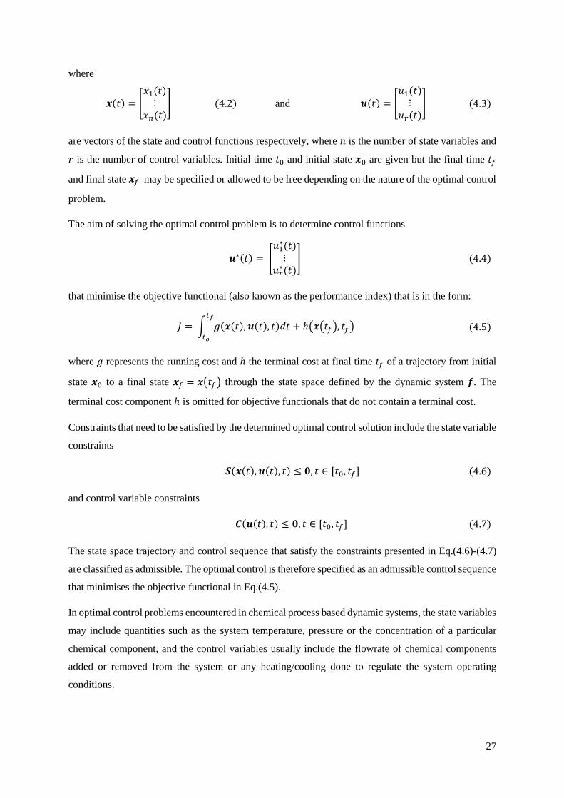
27

where

𝒙(𝑡) = [𝑥1(𝑡)

⋮𝑥𝑛(𝑡)

] (4.2) and 𝒖(𝑡) = [𝑢1(𝑡)

⋮𝑢𝑟(𝑡)

] (4.3)

are vectors of the state and control functions respectively, where 𝑛 is the number of state variables and

𝑟 is the number of control variables. Initial time 𝑡0 and initial state 𝒙0 are given but the final time 𝑡𝑓

and final state 𝒙𝑓 may be specified or allowed to be free depending on the nature of the optimal control

problem.

The aim of solving the optimal control problem is to determine control functions

that minimise the objective functional (also known as the performance index) that is in the form:

where 𝑔 represents the running cost and ℎ the terminal cost at final time 𝑡𝑓 of a trajectory from initial

state 𝒙0 to a final state 𝒙𝑓 = 𝒙(𝑡𝑓) through the state space defined by the dynamic system 𝒇. The

terminal cost component ℎ is omitted for objective functionals that do not contain a terminal cost.

Constraints that need to be satisfied by the determined optimal control solution include the state variable

constraints

𝑺(𝒙(𝑡), 𝒖(𝑡), 𝑡) ≤ 𝟎, 𝑡 ∈ [𝑡0, 𝑡𝑓] (4.6)

and control variable constraints

𝑪(𝒖(𝑡), 𝑡) ≤ 𝟎, 𝑡 ∈ [𝑡0, 𝑡𝑓] (4.7)

The state space trajectory and control sequence that satisfy the constraints presented in Eq.(4.6)-(4.7)

are classified as admissible. The optimal control is therefore specified as an admissible control sequence

that minimises the objective functional in Eq.(4.5).

In optimal control problems encountered in chemical process based dynamic systems, the state variables

may include quantities such as the system temperature, pressure or the concentration of a particular

chemical component, and the control variables usually include the flowrate of chemical components

added or removed from the system or any heating/cooling done to regulate the system operating

conditions.

𝒖∗(𝑡) = [𝑢1

∗(𝑡)⋮

𝑢𝑟∗(𝑡)

] (4.4)

𝐽 = ∫ 𝑔(𝒙(𝑡), 𝒖(𝑡), 𝑡)𝑑𝑡𝑡𝑓

𝑡𝑜

+ ℎ(𝒙(𝑡𝑓), 𝑡𝑓) (4.5)

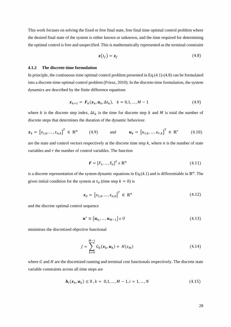
28

This work focuses on solving the fixed or free final state, free final time optimal control problem where

the desired final state of the system is either known or unknown, and the time required for determining

the optimal control is free and unspecified. This is mathematically represented as the terminal constraint

𝒙(𝑡𝑓) = 𝒙𝑓 (4.8)

4.1.2 The discrete-time formulation

In principle, the continuous-time optimal control problem presented in Eq.(4.1)-(4.8) can be formulated

into a discrete-time optimal control problem (Friesz, 2010). In the discrete-time formulation, the system

dynamics are described by the finite difference equations

where 𝑘 is the discrete step index, Δ𝑡𝑘 is the time for discrete step 𝑘 and 𝑀 is total the number of

discrete steps that determines the duration of the dynamic behaviour.

𝒙𝑘 = [𝑥1,𝑘, … , 𝑥𝑛,𝑘]𝑇

∈ ℝ𝑛 (4.9) and 𝒖𝑘 = [𝑢1,𝑘, … , 𝑢𝑟,𝑘]𝑇

∈ ℝ𝑟 (4.10)

are the state and control vectors respectively at the discrete time step 𝑘, where 𝑛 is the number of state

variables and 𝑟 the number of control variables. The function

is a discrete representation of the system dynamic equations in Eq.(4.1) and is differentiable in ℝ𝑛. The

given initial condition for the system at 𝑡0 (time step 𝑘 = 0) is

and the discrete optimal control sequence

minimises the discretized objective functional

where 𝐺 and 𝐻 are the discretized running and terminal cost functionals respectively. The discrete state

variable constraints across all time steps are

𝒙𝑘+1 = 𝑭𝑘(𝒙𝑘, 𝒖𝑘 , Δ𝑡𝑘), 𝑘 = 0,1, … , 𝑀 − 1 (4.9)

𝑭 = [𝐹1, … , 𝐹𝑛]𝑇 𝜖 ℝ𝑛 (4.11)

𝒙0 = [𝑥1,0, … , 𝑥𝑛,0]𝑇

∈ ℝ𝑛 (4.12)

𝒖∗ ≡ {𝒖0,, … , 𝒖𝑀−1} 𝜖 𝑈 (4.13)

𝐽 = ∑ 𝐺𝑘(𝒙𝑘, 𝒖𝑘)

𝑀−1

𝑘=0

+ 𝐻(𝑥𝑀) (4.14)

𝒉𝑖(𝒙𝑘 , 𝒖𝑘) ≤ 0 , 𝑘 = 0,1, … , 𝑀 − 1, 𝑖 = 1, … , 𝑁 (4.15)

29

where 𝒉𝑖, 𝑖 = 1, … , 𝑁 are given real valued functions in ℝ𝑛 × ℝ𝑟 and the control variable constraints

are addressed by defining a set of feasible controls

that can be applied to the system at time step 𝑘 where 𝑎𝑖 and 𝑏𝑖 are real numbers for given constraints

on the control input for each control variable 𝑢𝑖. It is noted that 𝑈 is a compact and convex subset of

ℝ𝑟.

A feasible control sequence

that results in the discrete state trajectory

when substituted to the finite difference equation in Eq.(4.9) while satisfying the initial condition in

Eq.(4.12) and Eq.(4.15)-(4.16) is termed an admissible control. The discrete optimal control 𝒖∗ is

therefore an admissible control that minimises the discrete objective functional in Eq.(4.14)

The terminal boundary condition for the fixed final state problem expressed as

where 𝑀 is free and determined by the discrete time steps taken by the optimal control solution to make

the system reach the desired final state 𝒙𝑀.

4.1.3 The optimal control solution

The objective of optimal control problem (see in 4.2.1) is to determine the optimal control action 𝒖∗(𝑡)

that results in the minimum objective functional 𝐽∗. Applying 𝒖∗(𝑡) to the system by substituting the

function into the differential equations for the dynamic system and integrating results in the optimal

state space trajectory 𝒙∗(𝑡).

Taking the two state variable optimal control problem from Kirk (2004), Example 5.1-1 (pages 198-

202), with dynamic system equations

𝑈 = {𝒖𝑘 = [𝑢1,𝑘, … , 𝑢𝑟,𝑘]𝑇

∈ ℝ𝑟: 𝑎𝑖 ≤ 𝑢𝑖,𝑘 ≤ 𝑏𝑖 , 𝑖 = 1, … , 𝑟, 𝑘 = 0,1, … , 𝑀 − 1} (4.16)

𝒖 ≡ {𝒖0,, … , 𝒖𝑀−1} 𝜖 𝑈 (4.17)

𝑿 ≡ {𝒙𝟏, … , 𝒙𝑴} (4.18)

𝒙𝑀 = 𝒙𝑓 (4.19)

𝑑𝑥1

𝑑𝑡= 𝑥2 (4.20)

𝑑𝑥2

𝑑𝑡= −𝑥2 + 𝑢 (4.21)

30

and the objective functional

with boundary constraints

𝒙𝟎 = [0, 0] (4.23) and 𝒙𝑭 = [5 , 2] (4.24)

The plots of the optimal control solution trajectories 𝑥1 𝑣𝑠 𝑡, 𝑥2 vs 𝑡, 𝑥1 𝑣𝑠 𝑥2 and optimal control 𝑢 vs 𝑡

for this problem are presented in Figure 4.1-4.3

Figure 4.1: Optimal control solution trajectories for x1 vs t and x2 vs t

The optimal state space trajectory in Figure 4.2 can be discretized by representing the state space as a

set of discrete state points and defining the discrete optimal state trajectory as a sequence of discrete

transitions through these points, from initial point 𝒙𝟎 = [0, 0] to final point 𝒙𝑭 = [5 , 2]. This trajectory

can be redefined as the discrete shortest path, with respect to the objective functional 𝐽, taken by the

system through the state space from 𝒙𝟎 to 𝒙𝑭. This is presented graphically in Figure 4.4. Plotting a set

of discrete points that lie in this shortest path trajectory (see Figure 4.5), the shortest state space path

from 𝒙𝟎 to 𝒙𝑭 can be approximated as the discrete path

𝐽 = 0.5 ∫1

2𝑢2𝑑𝑡

𝑡𝑓

0

(4.22)

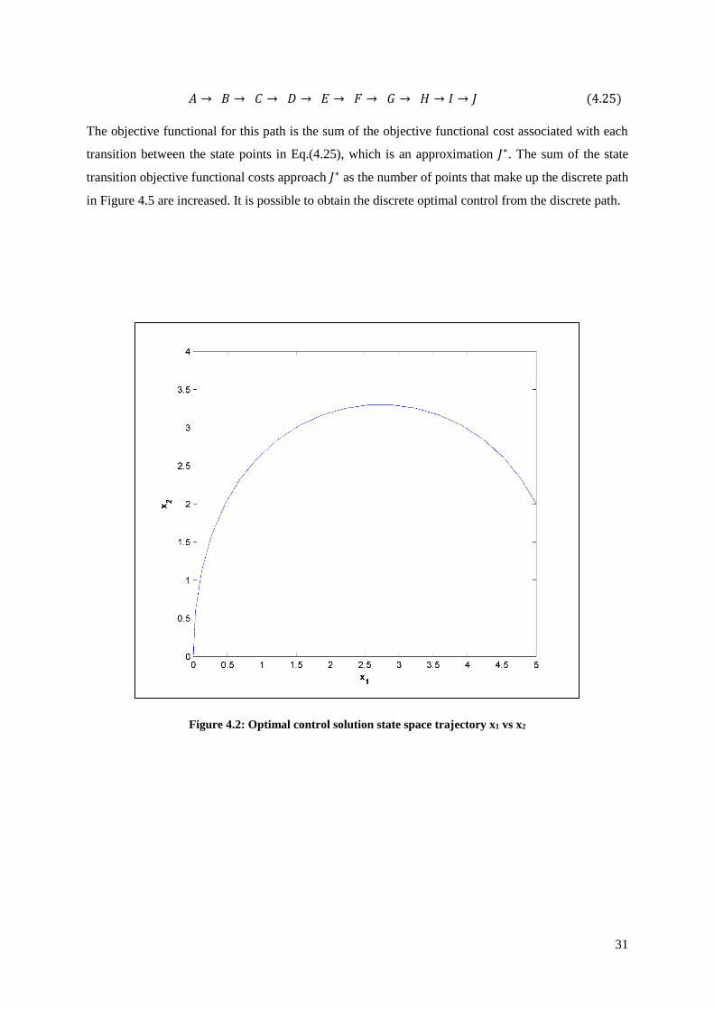
31

The objective functional for this path is the sum of the objective functional cost associated with each

transition between the state points in Eq.(4.25), which is an approximation 𝐽∗. The sum of the state

transition objective functional costs approach 𝐽∗ as the number of points that make up the discrete path

in Figure 4.5 are increased. It is possible to obtain the discrete optimal control from the discrete path.

Figure 4.2: Optimal control solution state space trajectory x1 vs x2

𝐴 → 𝐵 → 𝐶 → 𝐷 → 𝐸 → 𝐹 → 𝐺 → 𝐻 → 𝐼 → 𝐽 (4.25)

32

Figure 4.3: Optimal control trajectory u vs t

Figure 4.4: Optimal state space trajectory on a discrete state space

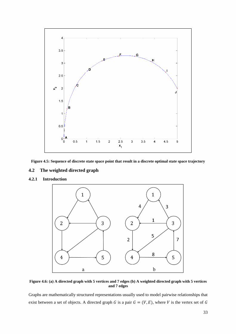
33

Figure 4.5: Sequence of discrete state space point that result in a discrete optimal state space trajectory

4.2 The weighted directed graph

4.2.1 Introduction

Figure 4.6: (a) A directed graph with 5 vertices and 7 edges (b) A weighted directed graph with 5 vertices

and 7 edges

Graphs are mathematically structured representations usually used to model pairwise relationships that

exist between a set of objects. A directed graph 𝐺 is a pair 𝐺 = (𝑉, 𝐸), where 𝑉 is the vertex set of 𝐺

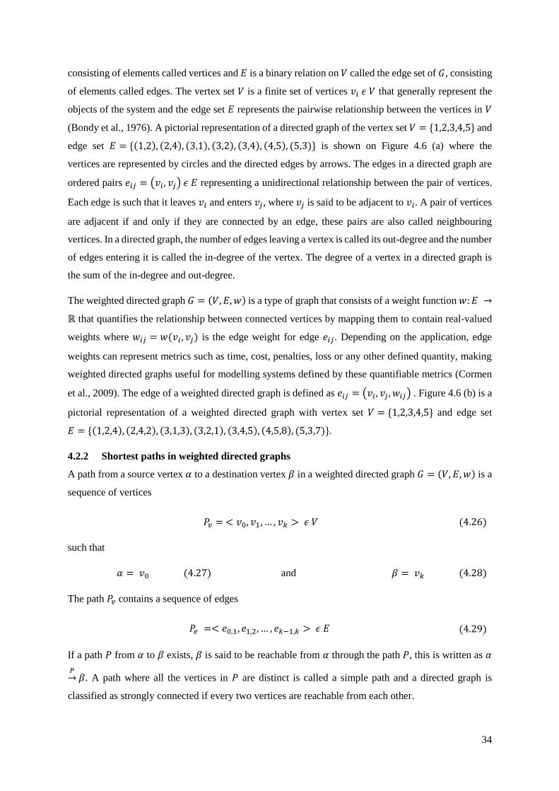
34

consisting of elements called vertices and 𝐸 is a binary relation on 𝑉 called the edge set of 𝐺, consisting

of elements called edges. The vertex set 𝑉 is a finite set of vertices 𝑣𝑖 𝜖 𝑉 that generally represent the

objects of the system and the edge set 𝐸 represents the pairwise relationship between the vertices in 𝑉

(Bondy et al., 1976). A pictorial representation of a directed graph of the vertex set 𝑉 = {1,2,3,4,5} and

edge set 𝐸 = {(1,2), (2,4), (3,1), (3,2), (3,4), (4,5), (5,3)} is shown on Figure 4.6 (a) where the

vertices are represented by circles and the directed edges by arrows. The edges in a directed graph are

ordered pairs 𝑒𝑖𝑗 = (𝑣𝑖, 𝑣𝑗) 𝜖 𝐸 representing a unidirectional relationship between the pair of vertices.

Each edge is such that it leaves 𝑣𝑖 and enters 𝑣𝑗, where 𝑣𝑗 is said to be adjacent to 𝑣𝑖. A pair of vertices

are adjacent if and only if they are connected by an edge, these pairs are also called neighbouring

vertices. In a directed graph, the number of edges leaving a vertex is called its out-degree and the number

of edges entering it is called the in-degree of the vertex. The degree of a vertex in a directed graph is

the sum of the in-degree and out-degree.

The weighted directed graph 𝐺 = (𝑉, 𝐸, 𝑤) is a type of graph that consists of a weight function 𝑤: 𝐸 →

ℝ that quantifies the relationship between connected vertices by mapping them to contain real-valued

weights where 𝑤𝑖𝑗 = 𝑤(𝑣𝑖 , 𝑣𝑗) is the edge weight for edge 𝑒𝑖𝑗. Depending on the application, edge

weights can represent metrics such as time, cost, penalties, loss or any other defined quantity, making

weighted directed graphs useful for modelling systems defined by these quantifiable metrics (Cormen

et al., 2009). The edge of a weighted directed graph is defined as 𝑒𝑖𝑗 = (𝑣𝑖, 𝑣𝑗 , 𝑤𝑖𝑗) . Figure 4.6 (b) is a

pictorial representation of a weighted directed graph with vertex set 𝑉 = {1,2,3,4,5} and edge set

𝐸 = {(1,2,4), (2,4,2), (3,1,3), (3,2,1), (3,4,5), (4,5,8), (5,3,7)}.

4.2.2 Shortest paths in weighted directed graphs

A path from a source vertex 𝛼 to a destination vertex 𝛽 in a weighted directed graph 𝐺 = (𝑉, 𝐸, 𝑤) is a

sequence of vertices

such that

𝛼 = 𝑣0 (4.27) and 𝛽 = 𝑣𝑘 (4.28)

The path 𝑃𝑣 contains a sequence of edges

If a path 𝑃 from 𝛼 to 𝛽 exists, 𝛽 is said to be reachable from 𝛼 through the path 𝑃, this is written as 𝛼

𝑃→ 𝛽. A path where all the vertices in 𝑃 are distinct is called a simple path and a directed graph is

classified as strongly connected if every two vertices are reachable from each other.

𝑃𝑣 = < 𝑣0, 𝑣1, … , 𝑣𝑘 > 𝜖 𝑉 (4.26)

𝑃𝑒 =< 𝑒0,1, 𝑒1,2, … , 𝑒𝑘−1,𝑘 > 𝜖 𝐸 (4.29)

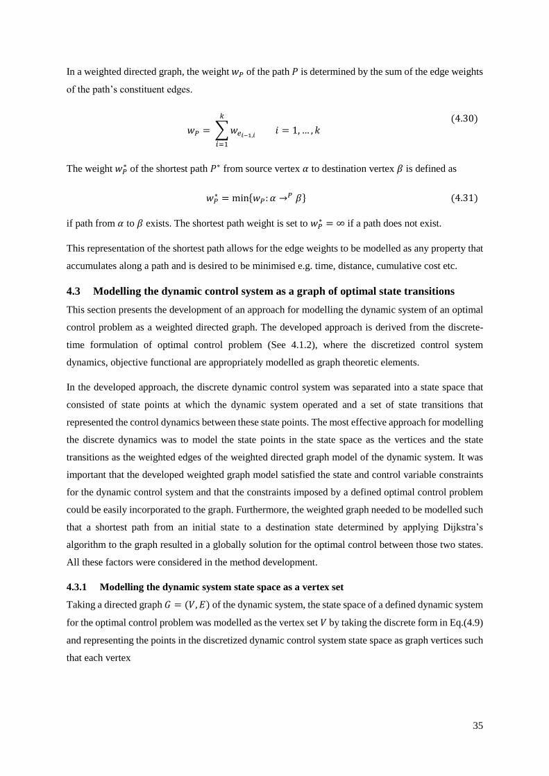
35

In a weighted directed graph, the weight 𝑤𝑃 of the path 𝑃 is determined by the sum of the edge weights

of the path’s constituent edges.

The weight 𝑤𝑃∗ of the shortest path 𝑃∗ from source vertex 𝛼 to destination vertex 𝛽 is defined as

if path from 𝛼 to 𝛽 exists. The shortest path weight is set to 𝑤𝑃∗ = ∞ if a path does not exist.

This representation of the shortest path allows for the edge weights to be modelled as any property that

accumulates along a path and is desired to be minimised e.g. time, distance, cumulative cost etc.

4.3 Modelling the dynamic control system as a graph of optimal state transitions

This section presents the development of an approach for modelling the dynamic system of an optimal

control problem as a weighted directed graph. The developed approach is derived from the discrete-

time formulation of optimal control problem (See 4.1.2), where the discretized control system

dynamics, objective functional are appropriately modelled as graph theoretic elements.

In the developed approach, the discrete dynamic control system was separated into a state space that

consisted of state points at which the dynamic system operated and a set of state transitions that

represented the control dynamics between these state points. The most effective approach for modelling

the discrete dynamics was to model the state points in the state space as the vertices and the state

transitions as the weighted edges of the weighted directed graph model of the dynamic system. It was

important that the developed weighted graph model satisfied the state and control variable constraints

for the dynamic control system and that the constraints imposed by a defined optimal control problem

could be easily incorporated to the graph. Furthermore, the weighted graph needed to be modelled such

that a shortest path from an initial state to a destination state determined by applying Dijkstra’s

algorithm to the graph resulted in a globally solution for the optimal control between those two states.

All these factors were considered in the method development.

4.3.1 Modelling the dynamic system state space as a vertex set

Taking a directed graph 𝐺 = (𝑉, 𝐸) of the dynamic system, the state space of a defined dynamic system

for the optimal control problem was modelled as the vertex set 𝑉 by taking the discrete form in Eq.(4.9)

and representing the points in the discretized dynamic control system state space as graph vertices such

that each vertex

𝑤𝑃 = ∑ 𝑤𝑒𝑖−1,𝑖

𝑘

𝑖=1

𝑖 = 1, … , 𝑘 (4.30)

𝑤𝑃∗ = min{𝑤𝑃: 𝛼 →𝑃 𝛽} (4.31)

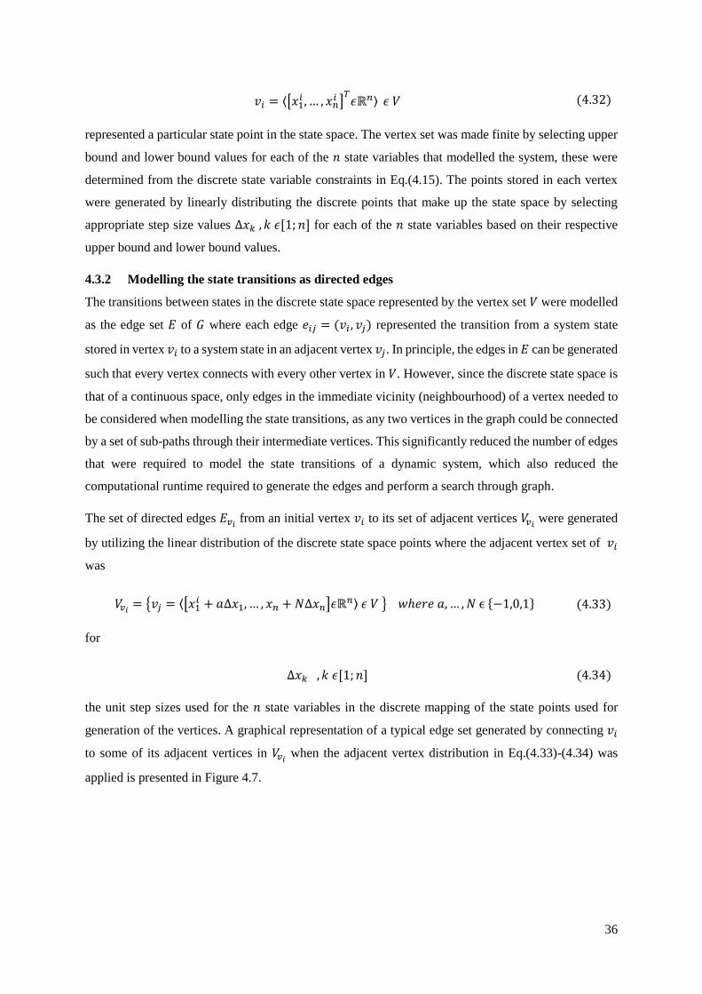
36

represented a particular state point in the state space. The vertex set was made finite by selecting upper

bound and lower bound values for each of the 𝑛 state variables that modelled the system, these were

determined from the discrete state variable constraints in Eq.(4.15). The points stored in each vertex

were generated by linearly distributing the discrete points that make up the state space by selecting

appropriate step size values Δ𝑥𝑘 , 𝑘 𝜖[1; 𝑛] for each of the 𝑛 state variables based on their respective

upper bound and lower bound values.

4.3.2 Modelling the state transitions as directed edges

The transitions between states in the discrete state space represented by the vertex set 𝑉 were modelled

as the edge set 𝐸 of 𝐺 where each edge 𝑒𝑖𝑗 = (𝑣𝑖 , 𝑣𝑗) represented the transition from a system state

stored in vertex 𝑣𝑖 to a system state in an adjacent vertex 𝑣𝑗. In principle, the edges in 𝐸 can be generated

such that every vertex connects with every other vertex in 𝑉. However, since the discrete state space is

that of a continuous space, only edges in the immediate vicinity (neighbourhood) of a vertex needed to

be considered when modelling the state transitions, as any two vertices in the graph could be connected

by a set of sub-paths through their intermediate vertices. This significantly reduced the number of edges

that were required to model the state transitions of a dynamic system, which also reduced the

computational runtime required to generate the edges and perform a search through graph.

The set of directed edges 𝐸𝑣𝑖 from an initial vertex 𝑣𝑖 to its set of adjacent vertices 𝑉𝑣𝑖

were generated

by utilizing the linear distribution of the discrete state space points where the adjacent vertex set of 𝑣𝑖

was

for

the unit step sizes used for the 𝑛 state variables in the discrete mapping of the state points used for

generation of the vertices. A graphical representation of a typical edge set generated by connecting 𝑣𝑖

to some of its adjacent vertices in 𝑉𝑣𝑖 when the adjacent vertex distribution in Eq.(4.33)-(4.34) was

applied is presented in Figure 4.7.

𝑣𝑖 = ⟨[𝑥1𝑖 , … , 𝑥𝑛

𝑖 ]𝑇

𝜖ℝ𝑛⟩ 𝜖 𝑉 (4.32)

𝑉𝑣𝑖= {𝑣𝑗 = ⟨[𝑥1

𝑖 + 𝑎∆𝑥1, … , 𝑥𝑛 + 𝑁∆𝑥𝑛]𝜖ℝ𝑛⟩ 𝜖 𝑉 } 𝑤ℎ𝑒𝑟𝑒 𝑎, … , 𝑁 ϵ {−1,0,1} (4.33)

Δ𝑥𝑘 , 𝑘 𝜖[1; 𝑛] (4.34)

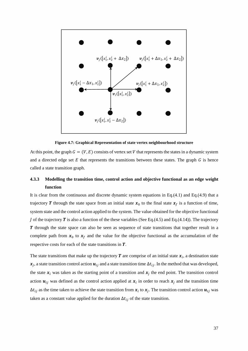
37

Figure 4.7: Graphical Representation of state vertex neighbourhood structure

At this point, the graph 𝐺 = (𝑉, 𝐸) consists of vertex set 𝑉 that represents the states in a dynamic system

and a directed edge set 𝐸 that represents the transitions between these states. The graph 𝐺 is hence

called a state transition graph.

4.3.3 Modelling the transition time, control action and objective functional as an edge weight

function

It is clear from the continuous and discrete dynamic system equations in Eq.(4.1) and Eq.(4.9) that a

trajectory 𝑻 through the state space from an initial state 𝒙0 to the final state 𝒙𝑓 is a function of time,

system state and the control action applied to the system. The value obtained for the objective functional

𝐽 of the trajectory 𝑻 is also a function of the these variables (See Eq.(4.5) and Eq.(4.14)). The trajectory

𝑻 through the state space can also be seen as sequence of state transitions that together result in a

complete path from 𝒙0 to 𝒙𝑓 and the value for the objective functional as the accumulation of the

respective costs for each of the state transitions in 𝑻.

The state transitions that make up the trajectory 𝑻 are comprise of an initial state 𝒙𝑖, a destination state

𝒙𝑗, a state transition control action 𝒖𝑖𝑗 and a state transition time Δ𝑡𝑖𝑗. In the method that was developed,

the state 𝒙𝑖 was taken as the starting point of a transition and 𝒙𝑗 the end point. The transition control

action 𝒖𝑖𝑗 was defined as the control action applied at 𝒙𝑖 in order to reach 𝒙𝑗 and the transition time

Δ𝑡𝑖𝑗 as the time taken to achieve the state transition from 𝒙𝑖 to 𝒙𝑗. The transition control action 𝒖𝑖𝑗 was

taken as a constant value applied for the duration Δ𝑡𝑖𝑗 of the state transition.

𝒗𝑖⟨[𝑥1𝑖 , 𝑥2

𝑖 ]⟩

𝒗𝑗⟨[𝑥1𝑖 + ∆𝑥1, 𝑥2

𝑖 ]⟩

𝒗𝑗⟨[𝑥1𝑖 , 𝑥2

𝑖 + ∆𝑥2]⟩

𝒗𝑗⟨[𝑥1𝑖 − ∆𝑥1, 𝑥2

𝑖 ]⟩

𝒗𝑗⟨[𝑥1𝑖 , 𝑥2

𝑖 − ∆𝑥2]⟩

𝒗𝑗⟨[𝑥1𝑖 + ∆𝑥1, 𝑥2

𝑖 + ∆𝑥2]⟩

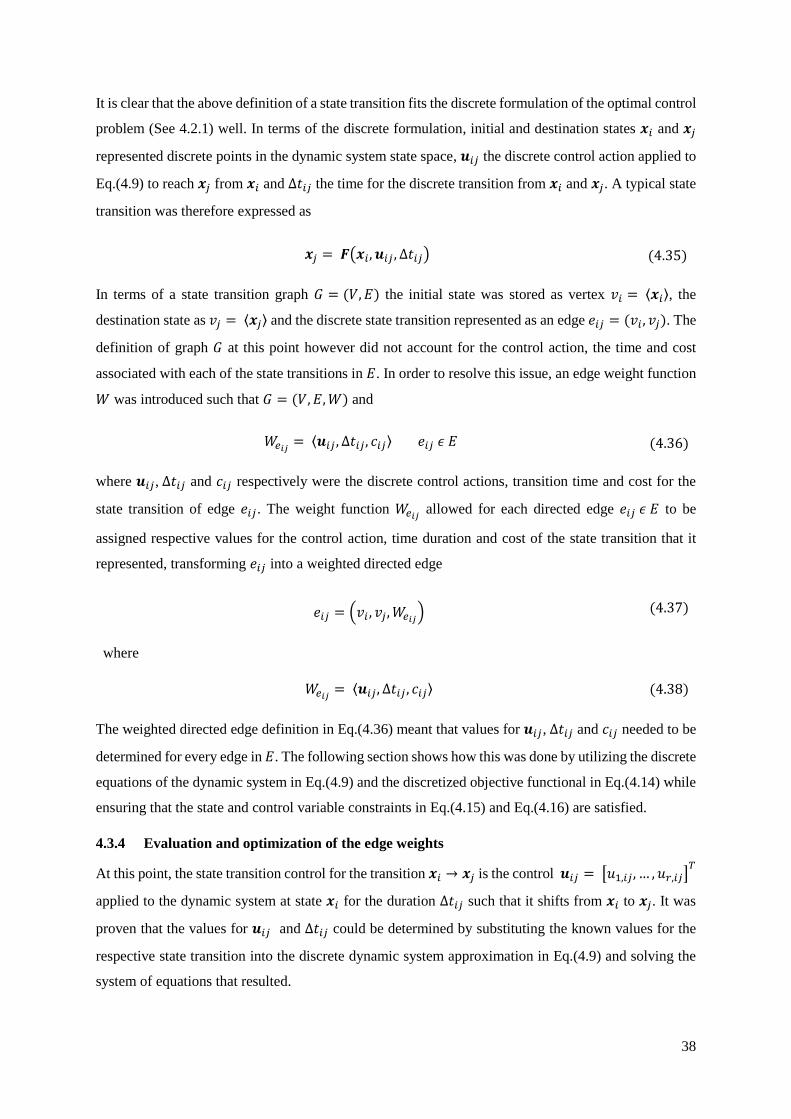
38

It is clear that the above definition of a state transition fits the discrete formulation of the optimal control

problem (See 4.2.1) well. In terms of the discrete formulation, initial and destination states 𝒙𝑖 and 𝒙𝑗

represented discrete points in the dynamic system state space, 𝒖𝑖𝑗 the discrete control action applied to

Eq.(4.9) to reach 𝒙𝑗 from 𝒙𝑖 and Δ𝑡𝑖𝑗 the time for the discrete transition from 𝒙𝑖 and 𝒙𝑗. A typical state

transition was therefore expressed as

In terms of a state transition graph 𝐺 = (𝑉, 𝐸) the initial state was stored as vertex 𝑣𝑖 = ⟨𝒙𝑖⟩, the

destination state as 𝑣𝑗 = ⟨𝒙𝑗⟩ and the discrete state transition represented as an edge 𝑒𝑖𝑗 = (𝑣𝑖 , 𝑣𝑗). The

definition of graph 𝐺 at this point however did not account for the control action, the time and cost

associated with each of the state transitions in 𝐸. In order to resolve this issue, an edge weight function

𝑊 was introduced such that 𝐺 = (𝑉, 𝐸, 𝑊) and

where 𝒖𝑖𝑗, Δ𝑡𝑖𝑗 and 𝑐𝑖𝑗 respectively were the discrete control actions, transition time and cost for the

state transition of edge 𝑒𝑖𝑗. The weight function 𝑊𝑒𝑖𝑗 allowed for each directed edge 𝑒𝑖𝑗 𝜖 𝐸 to be

assigned respective values for the control action, time duration and cost of the state transition that it

represented, transforming 𝑒𝑖𝑗 into a weighted directed edge

The weighted directed edge definition in Eq.(4.36) meant that values for 𝒖𝑖𝑗, Δ𝑡𝑖𝑗 and 𝑐𝑖𝑗 needed to be

determined for every edge in 𝐸. The following section shows how this was done by utilizing the discrete

equations of the dynamic system in Eq.(4.9) and the discretized objective functional in Eq.(4.14) while

ensuring that the state and control variable constraints in Eq.(4.15) and Eq.(4.16) are satisfied.

4.3.4 Evaluation and optimization of the edge weights

At this point, the state transition control for the transition 𝒙𝑖 → 𝒙𝑗 is the control 𝒖𝑖𝑗 = [𝑢1,𝑖𝑗, … , 𝑢𝑟,𝑖𝑗]𝑇

applied to the dynamic system at state 𝒙𝑖 for the duration Δ𝑡𝑖𝑗 such that it shifts from 𝒙𝑖 to 𝒙𝑗. It was

proven that the values for 𝒖𝑖𝑗 and Δ𝑡𝑖𝑗 could be determined by substituting the known values for the

respective state transition into the discrete dynamic system approximation in Eq.(4.9) and solving the

system of equations that resulted.

𝒙𝑗 = 𝑭(𝒙𝑖, 𝒖𝑖𝑗 , Δ𝑡𝑖𝑗) (4.35)

𝑊𝑒𝑖𝑗= ⟨𝒖𝑖𝑗 , Δ𝑡𝑖𝑗, 𝑐𝑖𝑗⟩ 𝑒𝑖𝑗 𝜖 𝐸 (4.36)

𝑒𝑖𝑗 = (𝑣𝑖 , 𝑣𝑗, 𝑊𝑒𝑖𝑗)

where

(4.37)

𝑊𝑒𝑖𝑗= ⟨𝒖𝑖𝑗, Δ𝑡𝑖𝑗 , 𝑐𝑖𝑗⟩ (4.38)

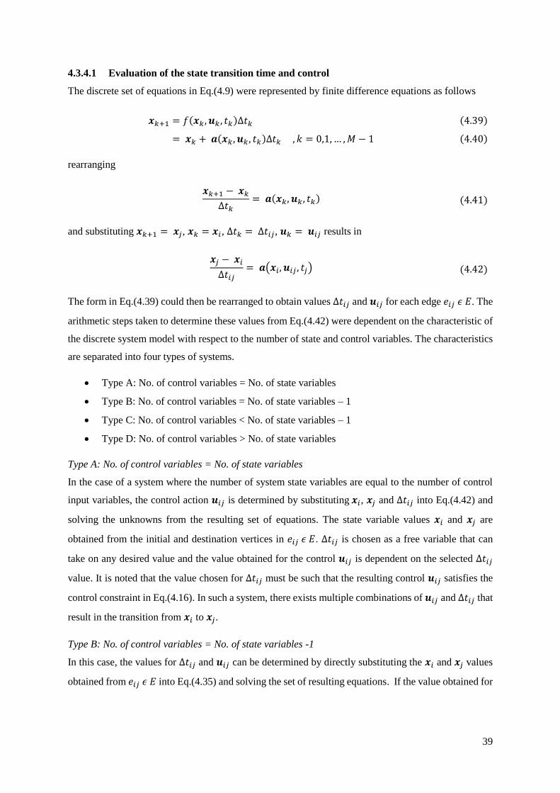
39

4.3.4.1 Evaluation of the state transition time and control

The discrete set of equations in Eq.(4.9) were represented by finite difference equations as follows

rearranging

and substituting 𝒙𝑘+1 = 𝒙𝑗, 𝒙𝑘 = 𝒙𝑖, Δ𝑡𝑘 = Δ𝑡𝑖𝑗, 𝒖𝑘 = 𝒖𝑖𝑗 results in

The form in Eq.(4.39) could then be rearranged to obtain values Δ𝑡𝑖𝑗 and 𝒖𝑖𝑗 for each edge 𝑒𝑖𝑗 𝜖 𝐸. The

arithmetic steps taken to determine these values from Eq.(4.42) were dependent on the characteristic of

the discrete system model with respect to the number of state and control variables. The characteristics

are separated into four types of systems.

• Type A: No. of control variables = No. of state variables

• Type B: No. of control variables = No. of state variables – 1

• Type C: No. of control variables < No. of state variables – 1

• Type D: No. of control variables > No. of state variables

Type A: No. of control variables = No. of state variables

In the case of a system where the number of system state variables are equal to the number of control

input variables, the control action 𝒖𝑖𝑗 is determined by substituting 𝒙𝑖, 𝒙𝑗 and Δ𝑡𝑖𝑗 into Eq.(4.42) and

solving the unknowns from the resulting set of equations. The state variable values 𝒙𝑖 and 𝒙𝑗 are

obtained from the initial and destination vertices in 𝑒𝑖𝑗 𝜖 𝐸. Δ𝑡𝑖𝑗 is chosen as a free variable that can

take on any desired value and the value obtained for the control 𝒖𝑖𝑗 is dependent on the selected Δ𝑡𝑖𝑗

value. It is noted that the value chosen for Δ𝑡𝑖𝑗 must be such that the resulting control 𝒖𝑖𝑗 satisfies the

control constraint in Eq.(4.16). In such a system, there exists multiple combinations of 𝒖𝑖𝑗 and Δ𝑡𝑖𝑗 that

result in the transition from 𝒙𝑖 to 𝒙𝑗.

Type B: No. of control variables = No. of state variables -1

In this case, the values for Δ𝑡𝑖𝑗 and 𝒖𝑖𝑗 can be determined by directly substituting the 𝒙𝑖 and 𝒙𝑗 values

obtained from 𝑒𝑖𝑗 𝜖 𝐸 into Eq.(4.35) and solving the set of resulting equations. If the value obtained for

𝒙𝑘+1 = 𝑓(𝒙𝑘 , 𝒖𝑘 , 𝑡𝑘)Δ𝑡𝑘

= 𝒙𝑘 + 𝒂(𝒙𝑘 , 𝒖𝑘 , 𝑡𝑘)Δ𝑡𝑘 , 𝑘 = 0,1, … , 𝑀 − 1

(4.39)

(4.40)

𝒙𝑘+1 − 𝒙𝑘

Δ𝑡𝑘= 𝒂(𝒙𝑘, 𝒖𝑘 , 𝑡𝑘) (4.41)

𝒙𝑗 − 𝒙𝑖

Δ𝑡𝑖𝑗= 𝒂(𝒙𝑖, 𝒖𝑖𝑗 , 𝑡𝑗) (4.42)

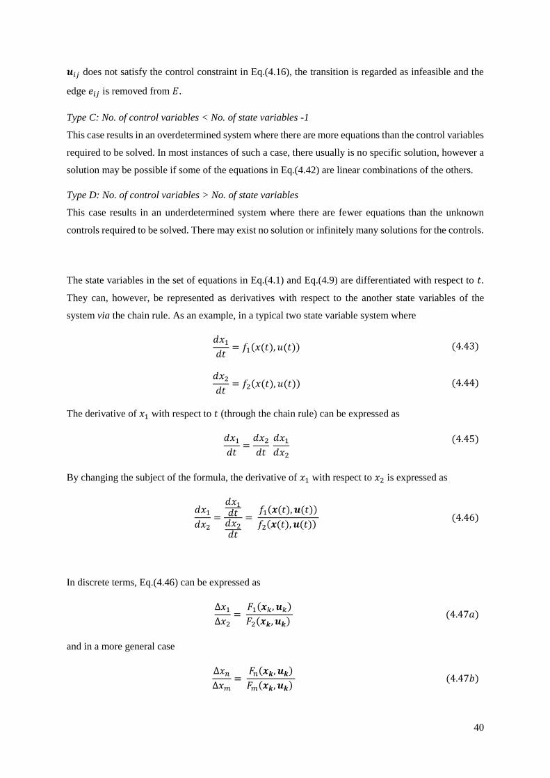
40

𝒖𝑖𝑗 does not satisfy the control constraint in Eq.(4.16), the transition is regarded as infeasible and the

edge 𝑒𝑖𝑗 is removed from 𝐸.

Type C: No. of control variables < No. of state variables -1

This case results in an overdetermined system where there are more equations than the control variables

required to be solved. In most instances of such a case, there usually is no specific solution, however a

solution may be possible if some of the equations in Eq.(4.42) are linear combinations of the others.

Type D: No. of control variables > No. of state variables

This case results in an underdetermined system where there are fewer equations than the unknown

controls required to be solved. There may exist no solution or infinitely many solutions for the controls.

The state variables in the set of equations in Eq.(4.1) and Eq.(4.9) are differentiated with respect to 𝑡.

They can, however, be represented as derivatives with respect to the another state variables of the

system via the chain rule. As an example, in a typical two state variable system where

𝑑𝑥1

𝑑𝑡= 𝑓1(𝑥(𝑡), 𝑢(𝑡)) (4.43)

𝑑𝑥2

𝑑𝑡= 𝑓2(𝑥(𝑡), 𝑢(𝑡)) (4.44)

The derivative of 𝑥1 with respect to 𝑡 (through the chain rule) can be expressed as

𝑑𝑥1

𝑑𝑡=

𝑑𝑥2

𝑑𝑡 𝑑𝑥1

𝑑𝑥2

(4.45)

By changing the subject of the formula, the derivative of 𝑥1 with respect to 𝑥2 is expressed as

𝑑𝑥1

𝑑𝑥2=

𝑑𝑥1𝑑𝑡

𝑑𝑥2𝑑𝑡

= 𝑓1(𝒙(𝑡), 𝒖(𝑡))

𝑓2(𝒙(𝑡), 𝒖(𝑡)) (4.46)

In discrete terms, Eq.(4.46) can be expressed as

Δ𝑥1

Δ𝑥2=

𝐹1(𝒙𝑘, 𝒖𝑘)

𝐹2(𝒙𝒌, 𝒖𝒌) (4.47𝑎)

and in a more general case

Δ𝑥𝑛

Δ𝑥𝑚=

𝐹𝑛(𝒙𝒌, 𝒖𝒌)

𝐹𝑚(𝒙𝒌, 𝒖𝒌) (4.47𝑏)

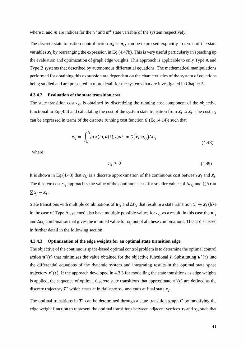
41

where 𝑛 and 𝑚 are indices for the nth and mth state variable of the system respectively.

The discrete state transition control action 𝒖𝒌 = 𝒖𝑖𝑗 can be expressed explicitly in terms of the state

variables 𝒙𝑘 by rearranging the expression in Eq.(4.47b). This is very useful particularly in speeding up

the evaluation and optimization of graph edge weights. This approach is applicable to only Type A and

Type B systems that described by autonomous differential equations. The mathematical manipulations

performed for obtaining this expression are dependent on the characteristics of the system of equations

being studied and are presented in more detail for the systems that are investigated in Chapter 5.

4.3.4.2 Evaluation of the state transition cost

The state transition cost 𝑐𝑖𝑗 is obtained by discretizing the running cost component of the objective

functional in Eq.(4.5) and calculating the cost of the system state transition from 𝒙𝑖 to 𝒙𝑗. The cost 𝑐𝑖𝑗

can be expressed in terms of the discrete running cost function 𝐺 (Eq.(4.14)) such that

It is shown in Eq.(4.48) that 𝑐𝑖𝑗 is a discrete approximation of the continuous cost between 𝒙𝑖 and 𝒙𝑗.

The discrete cost 𝑐𝑖𝑗 approaches the value of the continuous cost for smaller values of Δ𝑡𝑖𝑗 and ∑ Δ𝒙 =

∑ 𝒙𝑗 − 𝒙𝑖 .

State transitions with multiple combinations of 𝒖𝑖𝑗 and Δ𝑡𝑖𝑗 that result in a state transition 𝒙𝑖 → 𝒙𝑗 (like

in the case of Type A systems) also have multiple possible values for 𝑐𝑖𝑗 as a result. In this case the 𝒖𝑖𝑗

and Δ𝑡𝑖𝑗 combination that gives the minimal value for 𝑐𝑖𝑗 out of all these combinations. This is discussed

in further detail in the following section.

4.3.4.3 Optimization of the edge weights for an optimal state transition edge

The objective of the continuous space-based optimal control problem is to determine the optimal control

action 𝒖∗(𝑡) that minimises the value obtained for the objective functional 𝐽. Substituting 𝒖∗(𝑡) into

the differential equations of the dynamic system and integrating results in the optimal state space

trajectory 𝒙∗(𝑡). If the approach developed in 4.3.3 for modelling the state transitions as edge weights

is applied, the sequence of optimal discrete state transitions that approximate 𝒙∗(𝑡) are defined as the

discrete trajectory 𝑻∗ which starts at initial state 𝒙0 and ends at final state 𝒙𝑓.

The optimal transitions in 𝑻∗ can be determined through a state transition graph 𝐺 by modifying the

edge weight function to represent the optimal transitions between adjacent vertices 𝒙𝑖 and 𝒙𝑗, such that

𝑐𝑖𝑗 = ∫ 𝑔(𝒙(𝑡), 𝒖(𝑡), 𝑡)𝑑𝑡𝑡𝒋

𝑡𝑖

≈ 𝐺(𝒙𝑖 , 𝒖𝑖𝑗)Δ𝑡𝑖𝑗

where

(4.48)

𝑐𝑖𝑗 ≥ 0 (4.49)

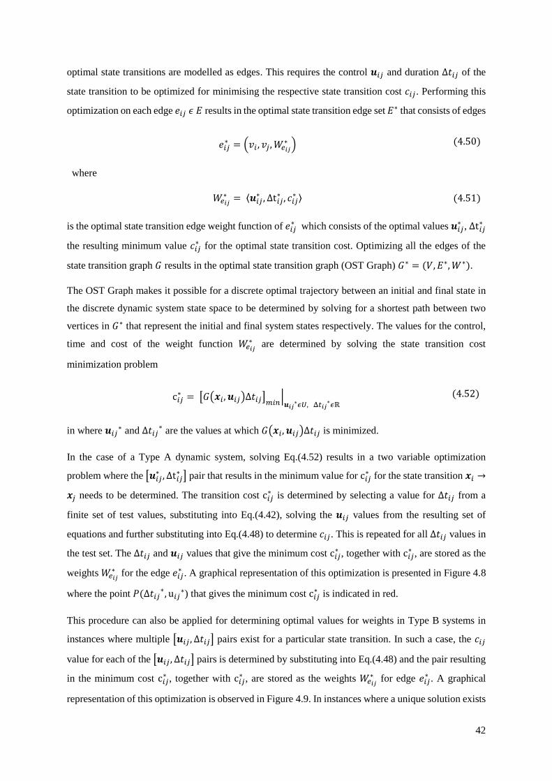
42

optimal state transitions are modelled as edges. This requires the control 𝒖𝑖𝑗 and duration Δ𝑡𝑖𝑗 of the

state transition to be optimized for minimising the respective state transition cost 𝑐𝑖𝑗. Performing this

optimization on each edge 𝑒𝑖𝑗 𝜖 𝐸 results in the optimal state transition edge set 𝐸∗ that consists of edges

is the optimal state transition edge weight function of 𝑒𝑖𝑗∗ which consists of the optimal values 𝒖𝑖𝑗

∗ , Δt𝑖𝑗∗

the resulting minimum value 𝑐𝑖𝑗∗ for the optimal state transition cost. Optimizing all the edges of the

state transition graph 𝐺 results in the optimal state transition graph (OST Graph) 𝐺∗ = (𝑉, 𝐸∗, 𝑊∗).

The OST Graph makes it possible for a discrete optimal trajectory between an initial and final state in

the discrete dynamic system state space to be determined by solving for a shortest path between two

vertices in 𝐺∗ that represent the initial and final system states respectively. The values for the control,

time and cost of the weight function 𝑊𝑒𝑖𝑗∗ are determined by solving the state transition cost

minimization problem

in where 𝒖𝑖𝑗∗ and Δ𝑡𝑖𝑗

∗ are the values at which 𝐺(𝒙𝑖, 𝒖𝑖𝑗)Δ𝑡𝑖𝑗 is minimized.

In the case of a Type A dynamic system, solving Eq.(4.52) results in a two variable optimization

problem where the [𝒖𝑖𝑗∗ , Δt𝑖𝑗

∗ ] pair that results in the minimum value for c𝑖𝑗∗ for the state transition 𝒙𝑖 →

𝒙𝑗 needs to be determined. The transition cost c𝑖𝑗∗ is determined by selecting a value for Δ𝑡𝑖𝑗 from a

finite set of test values, substituting into Eq.(4.42), solving the 𝒖𝑖𝑗 values from the resulting set of

equations and further substituting into Eq.(4.48) to determine 𝑐𝑖𝑗. This is repeated for all Δ𝑡𝑖𝑗 values in

the test set. The Δ𝑡𝑖𝑗 and 𝒖𝑖𝑗 values that give the minimum cost c𝑖𝑗∗ , together with c𝑖𝑗

∗ , are stored as the

weights 𝑊𝑒𝑖𝑗∗ for the edge 𝑒𝑖𝑗

∗ . A graphical representation of this optimization is presented in Figure 4.8

where the point 𝑃(Δ𝑡𝑖𝑗∗, u𝑖𝑗

∗) that gives the minimum cost c𝑖𝑗∗ is indicated in red.

This procedure can also be applied for determining optimal values for weights in Type B systems in

instances where multiple [𝒖𝑖𝑗 , Δ𝑡𝑖𝑗] pairs exist for a particular state transition. In such a case, the 𝑐𝑖𝑗

value for each of the [𝒖𝑖𝑗 , Δ𝑡𝑖𝑗] pairs is determined by substituting into Eq.(4.48) and the pair resulting

in the minimum cost c𝑖𝑗∗ , together with c𝑖𝑗

∗ , are stored as the weights 𝑊𝑒𝑖𝑗∗ for edge 𝑒𝑖𝑗

∗ . A graphical

representation of this optimization is observed in Figure 4.9. In instances where a unique solution exists

𝑒𝑖𝑗∗ = (𝑣𝑖 , 𝑣𝑗, 𝑊𝑒𝑖𝑗

∗ )

where

(4.50)

𝑊𝑒𝑖𝑗∗ = ⟨𝒖𝑖𝑗

∗ , Δt𝑖𝑗∗ , 𝑐𝑖𝑗

∗ ⟩ (4.51)

c𝑖𝑗∗ = [𝐺(𝒙𝑖, 𝒖𝑖𝑗)Δ𝑡𝑖𝑗]

𝑚𝑖𝑛|𝒖𝑖𝑗

∗𝜖𝑈, Δ𝑡𝑖𝑗∗𝜖ℝ

(4.52)

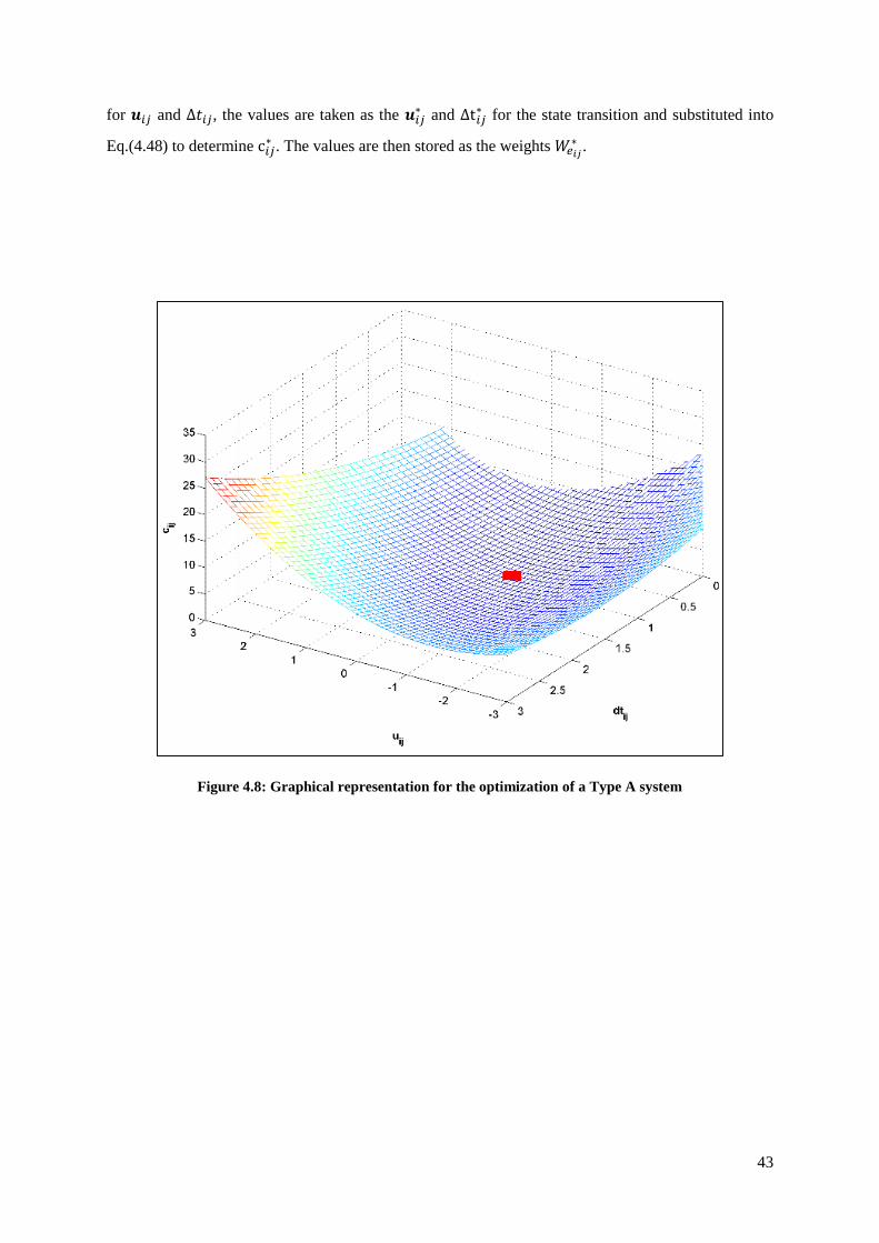
43

for 𝒖𝑖𝑗 and Δ𝑡𝑖𝑗, the values are taken as the 𝒖𝑖𝑗∗ and Δt𝑖𝑗

∗ for the state transition and substituted into

Eq.(4.48) to determine c𝑖𝑗∗ . The values are then stored as the weights 𝑊𝑒𝑖𝑗

∗ .

Figure 4.8: Graphical representation for the optimization of a Type A system

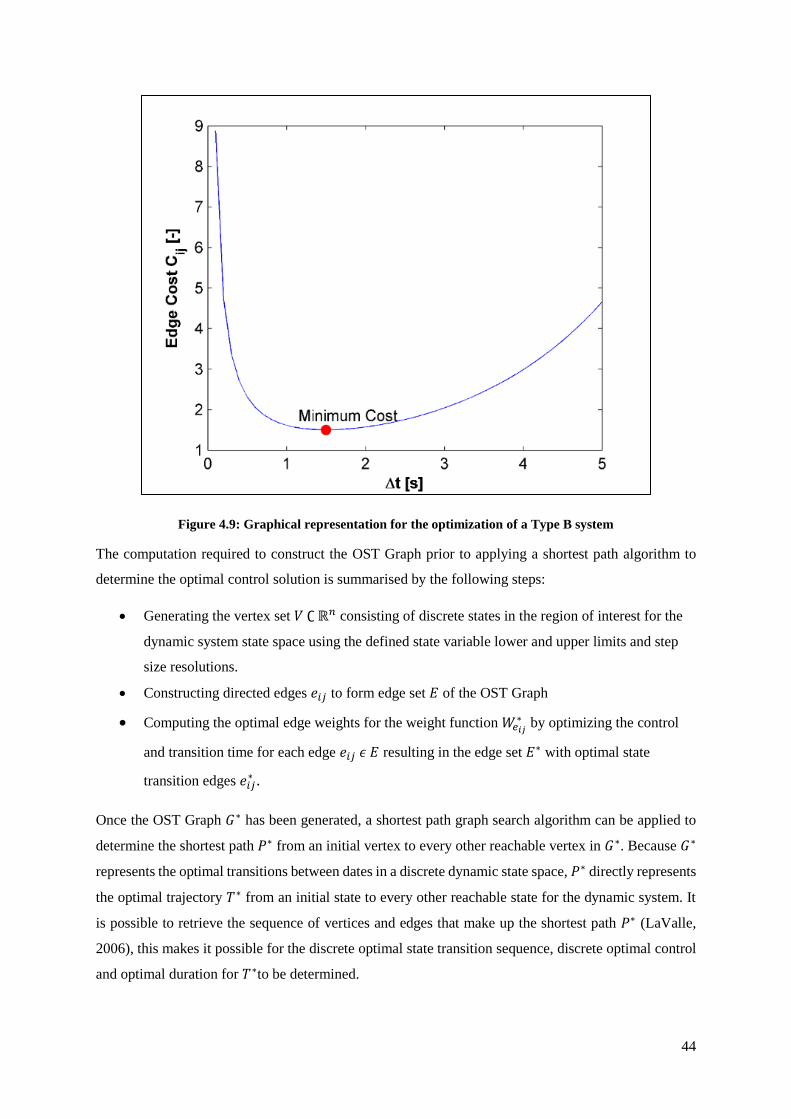
44

Figure 4.9: Graphical representation for the optimization of a Type B system

The computation required to construct the OST Graph prior to applying a shortest path algorithm to

determine the optimal control solution is summarised by the following steps:

• Generating the vertex set 𝑉 ∁ ℝ𝑛 consisting of discrete states in the region of interest for the

dynamic system state space using the defined state variable lower and upper limits and step

size resolutions.

• Constructing directed edges 𝑒𝑖𝑗 to form edge set 𝐸 of the OST Graph

• Computing the optimal edge weights for the weight function 𝑊𝑒𝑖𝑗∗ by optimizing the control

and transition time for each edge 𝑒𝑖𝑗 𝜖 𝐸 resulting in the edge set 𝐸∗ with optimal state

transition edges 𝑒𝑖𝑗∗ .

Once the OST Graph 𝐺∗ has been generated, a shortest path graph search algorithm can be applied to

determine the shortest path 𝑃∗ from an initial vertex to every other reachable vertex in 𝐺∗. Because 𝐺∗

represents the optimal transitions between dates in a discrete dynamic state space, 𝑃∗ directly represents

the optimal trajectory 𝑇∗ from an initial state to every other reachable state for the dynamic system. It

is possible to retrieve the sequence of vertices and edges that make up the shortest path 𝑃∗ (LaValle,

2006), this makes it possible for the discrete optimal state transition sequence, discrete optimal control

and optimal duration for 𝑇∗to be determined.

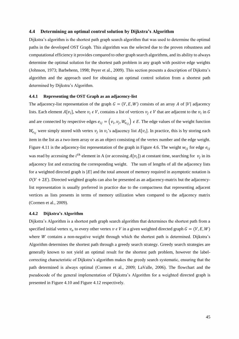
45

4.4 Determining an optimal control solution by Dijkstra’s Algorithm

Dijkstra’s algorithm is the shortest path graph search algorithm that was used to determine the optimal

paths in the developed OST Graph. This algorithm was the selected due to the proven robustness and

computational efficiency it provides compared to other graph search algorithms, and its ability to always

determine the optimal solution for the shortest path problem in any graph with positive edge weights

(Johnson, 1973; Barbehenn, 1998; Peyer et al., 2009). This section presents a description of Dijkstra’s

algorithm and the approach used for obtaining an optimal control solution from a shortest path

determined by Dijkstra’s Algorithm.

4.4.1 Representing the OST Graph as an adjacency-list

The adjacency-list representation of the graph 𝐺 = (𝑉, 𝐸, 𝑊) consists of an array 𝐴 of |𝑉| adjacency

lists. Each element 𝐴[𝑣𝑖], where 𝑣𝑖 𝜖 𝑉, contains a list of vertices 𝑣𝑗 𝜖 𝑉 that are adjacent to the 𝑣𝑖 in 𝐺

and are connected by respective edges 𝑒𝑖𝑗 = (𝑣𝑖 , 𝑣𝑗, 𝑊𝑒𝑖𝑗) 𝜖 𝐸. The edge values of the weight function

𝑊𝑒𝑖𝑗 were simply stored with vertex 𝑣𝑗 in 𝑣𝑖’s adjacency list 𝐴[𝑣𝑖]. In practice, this is by storing each

item in the list as a two-item array or as an object consisting of the vertex number and the edge weight.

Figure 4.11 is the adjacency-list representation of the graph in Figure 4.6. The weight 𝑤𝑖𝑗 for edge 𝑒𝑖𝑗

was read by accessing the 𝑖𝑡ℎ element in A (or accessing 𝐴[𝑣𝑖]) at constant time, searching for 𝑣𝑗 in its

adjacency list and extracting the corresponding weight. The sum of lengths of all the adjacency lists

for a weighted directed graph is |𝐸| and the total amount of memory required in asymptotic notation is

𝑂(𝑉 + 2𝐸). Directed weighted graphs can also be presented as an adjacency-matrix but the adjacency-

list representation is usually preferred in practice due to the compactness that representing adjacent

vertices as lists presents in terms of memory utilization when compared to the adjacency matrix

(Cormen et al., 2009).

4.4.2 Dijkstra’s Algorithm

Dijkstra’s Algorithm is a shortest path graph search algorithm that determines the shortest path from a

specified initial vertex 𝑣𝑜 to every other vertex 𝑣 𝜖 𝑉 in a given weighted directed graph 𝐺 = (𝑉, 𝐸, 𝑊)

where 𝑊 contains a non-negative weight through which the shortest path is determined. Dijkstra’s

Algorithm determines the shortest path through a greedy search strategy. Greedy search strategies are

generally known to not yield an optimal result for the shortest path problem, however the label-

correcting characteristic of Dijkstra’s algorithm makes the greedy search systematic, ensuring that the

path determined is always optimal (Cormen et al., 2009; LaValle, 2006). The flowchart and the

pseudocode of the general implementation of Dijkstra’s Algorithm for a weighted directed graph is

presented in Figure 4.10 and Figure 4.12 respectively.

46

Figure 4.10: Flowchart of Dijkstra's Algorithm

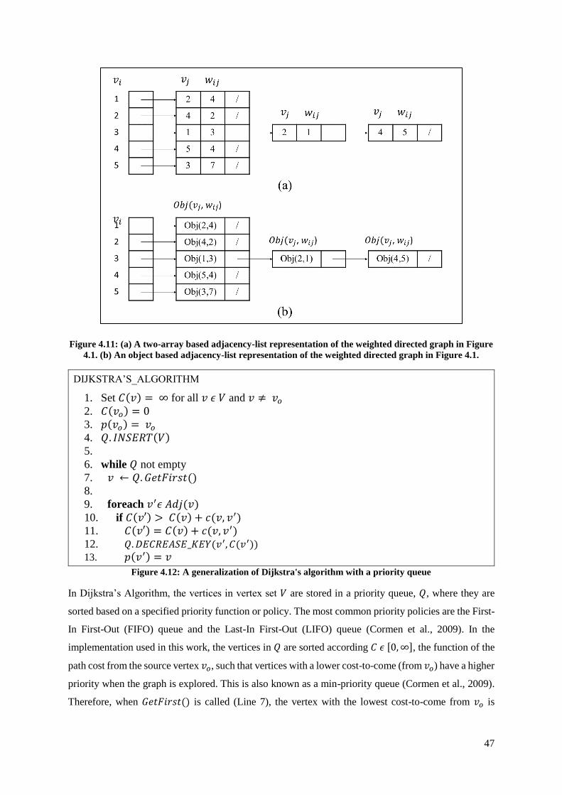
47

Figure 4.11: (a) A two-array based adjacency-list representation of the weighted directed graph in Figure

4.1. (b) An object based adjacency-list representation of the weighted directed graph in Figure 4.1.

DIJKSTRA’S_ALGORITHM

1. Set 𝐶(𝑣) = ∞ for all 𝑣 𝜖 𝑉 and 𝑣 ≠ 𝑣𝑜

2. 𝐶(𝑣𝑜) = 0

3. 𝑝(𝑣𝑜) = 𝑣𝑜

4. 𝑄. 𝐼𝑁𝑆𝐸𝑅𝑇(𝑉)

5. 6. while 𝑄 not empty

7. 𝑣 ← 𝑄. 𝐺𝑒𝑡𝐹𝑖𝑟𝑠𝑡()

8. 9. foreach 𝑣′𝜖 𝐴𝑑𝑗(𝑣)

10. if 𝐶(𝑣′) > 𝐶(𝑣) + 𝑐(𝑣, 𝑣′)

11. 𝐶(𝑣′) = 𝐶(𝑣) + 𝑐(𝑣, 𝑣′)

12. 𝑄. 𝐷𝐸𝐶𝑅𝐸𝐴𝑆𝐸_𝐾𝐸𝑌(𝑣′, 𝐶(𝑣′))

13. 𝑝(𝑣′) = 𝑣

Figure 4.12: A generalization of Dijkstra's algorithm with a priority queue

In Dijkstra’s Algorithm, the vertices in vertex set 𝑉 are stored in a priority queue, 𝑄, where they are

sorted based on a specified priority function or policy. The most common priority policies are the First-

In First-Out (FIFO) queue and the Last-In First-Out (LIFO) queue (Cormen et al., 2009). In the

implementation used in this work, the vertices in 𝑄 are sorted according 𝐶 𝜖 [0, ∞], the function of the

path cost from the source vertex 𝑣𝑜, such that vertices with a lower cost-to-come (from 𝑣𝑜) have a higher

priority when the graph is explored. This is also known as a min-priority queue (Cormen et al., 2009).

Therefore, when 𝐺𝑒𝑡𝐹𝑖𝑟𝑠𝑡() is called (Line 7), the vertex with the lowest cost-to-come from 𝑣𝑜 is

48

selected. The min-priority queue 𝑄 is initialized to only to contain all the vertices in 𝑉 prior to the

exploration and the computation of the path cost (from 𝑣𝑜) for all the vertices in the graph.

The computation of the shortest path costs is done through the execution of a while loop that terminates

only when 𝑄 is empty i.e. when all the vertices in 𝐺 have been explored. In each while loop iteration,

the vertex 𝑣 with the lowest cost-to-come 𝐶(𝑣) is removed from 𝑄 via the 𝐺𝑒𝑡𝐹𝑖𝑟𝑠𝑡() operation and

the cost-to-come 𝐶(𝑣′) of the adjacent vertices of 𝑣, 𝑣′𝜖 𝐴𝑑𝑗(𝑣), is evaluated and compared.

The path cost 𝐶(𝑣) for 𝑣 𝜖 𝑉, 𝑣 ≠ 𝑣𝑜 is computed incrementally as the while loop is executed. At each

while loop iteration, whenever an adjacent vertex 𝑣′ is reached through the exploration of vertex 𝑣, the

path cost (from 𝑣𝑜) for 𝑣′ is computed by 𝐶(𝑣) + 𝑐(𝑣, 𝑣′) where 𝑐(𝑣, 𝑣′) is the function that represents

the transition cost from 𝑣 to adjacent vertex 𝑣′. The value determined is compared with the existing

path cost 𝐶(𝑣′) and if the computed value is less than 𝐶(𝑣′), the path cost to 𝑣′ is updated by 𝐶(𝑣′) =

𝐶(𝑣) + 𝑐(𝑣, 𝑣′). The cost 𝐶(𝑣′) for 𝑣′ in 𝑄 is then updated via the 𝐷𝐸𝐶𝑅𝐸𝐴𝑆𝐸_𝐾𝐸𝑌(𝑣, 𝑣’) operation

and vertex 𝑣 is then stored as the predecessor of 𝑣′ (Line 12). After updating the cost 𝐶(𝑣′) for vertex

𝑣′ in 𝑄, the 𝐷𝐸𝐶𝑅𝐸𝐴𝑆𝐸_𝐾𝐸𝑌 operation also sorts the priority queue such that the vertex with the

minimum value 𝐶(𝑣) is the next accessible vertex when the 𝐺𝑒𝑡𝐹𝑖𝑟𝑠𝑡() operation is called in the next

loop iteration. Here, 𝐶(𝑣′) represents the lowest path cost known so far, which can be further updated

if a lower path cost is determined in future iterations. The cost-to-come 𝐶(𝑣) for all the vertices in

vertex set 𝑉 is initialized to infinity (Line 1), which updated when a lower value for 𝐶(𝑣) is determined

iterative computation through the graph.

It is only when all the vertices in 𝑉 have been explored and the min-priority queue 𝑄 is empty that the

cost-to-come for each vertex 𝑣 𝜖 𝑉 has an optimal value 𝐶∗(𝑣) for the optimal path 𝑃∗ (see 4.3.3) from

source vertex 𝑣𝑜. This optimal cost is equivalent to the summation of the edge costs 𝑐(𝑣, 𝑣′) in the path

𝑃∗ that is computed by Dijkstra’s algorithm. Therefore, 𝐶∗(𝑣𝐹) = ∞, 𝑣𝐹 𝜖 𝑉 for a selected destination

vertex 𝑣𝐹 implies that a path from 𝑣𝑜 to 𝑣𝐹 does not exist.

The sequence of vertices and of the optimal path 𝑃∗(𝑣𝑜, 𝑣𝐹) from 𝑣𝑜 to a selected destination vertex 𝑣𝐹

is determined by simply tracing the predecessor vertex pointers 𝑝(𝑣) from the selected final vertex 𝑣𝐹

back to the initial state 𝑣𝑜, resulting in the optimal path 𝑃∗(𝑣𝑜, 𝑣𝐹) = < 𝑣𝑜, … , 𝑣𝐹 >

Dijkstra’s algorithm guarantees the globally optimal result for the shortest path from a specified source

vertex and is known to provide the best computational runtime compared to other search algorithms if

correctly implemented (Peyer et al., 2009). An asymptotic running time of 𝑂(𝑉2) is achieved if the

vertices are stored as an array, however implementing a min-priority queue through a Binary min-heap

data structure improves this to 𝑂((𝑉 + 𝐸) log 𝑉). A further improved running time of 𝑂(𝑉 log 𝑉 + 𝐸)

can be obtained by implementing a Fibonacci heap however this improvement can be observed when

implemented on significantly dense graphs where 𝐸 ≫ 𝑣2 (Goldberg and Tarjan 1996).

49

4.4.3 Determining the optimal control solution by applying Dijkstra’s algorithm to the OST

Graph

The shortest path 𝑃∗(𝑣𝑜, 𝑣𝐹) in the OST Graph 𝐺∗ = (𝑉, 𝐸∗, 𝑊∗) is determined when Dijkstra’s

algorithm is applied to 𝐺∗ and a desired final vertex 𝑣𝐹 is selected. The optimal cost 𝐶∗(𝑣𝐹) for

𝑃∗(𝑣𝑜, 𝑣𝐹) can be expressed as

where 𝑖 = 0, … , 𝐹 is the sequence of vertices in the vertex set 𝑉 with 0 and 𝐹 representing the initial

and final vertex respectively.

As a result of the method developed for modelling a dynamic system as a graph of optimal state

transitions, 𝑃∗(𝑣𝑜, 𝑣𝐹) is can be said to be equivalent to 𝑇∗ = < 𝒙𝑜, … , 𝒙𝐹 > the optimal state space

trajectory solution of the discretized optimal control problem for shifting the system from initial state

𝒙𝑜 to a final state 𝒙𝐹.

The minimum value for the objective functional of the discrete optimal control problem solution can be

expressed as

where 𝐻(𝒙𝐹) is the specified terminal cost at state 𝒙𝐹.

The shortest path 𝑃∗(𝑣𝑜, 𝑣𝐹) can also be represented as a sequence of edges 𝑃∗(𝑣𝑜, 𝑣𝐹) =<

𝑒0,𝑖∗ , … , 𝑒𝑖,𝐹

∗ > where 𝑖 represents a vertex 𝑣𝑖𝜖𝑉. Utilizing this representation, the total time for the 𝑇∗

and hence the optimal control solution can be expressed as

where Δ𝑡𝑒𝑖−1,𝑖∗

∗ is the optimal state transition time for an edge 𝑒𝑖−1,𝑖∗ and 𝑖 = 1, … , 𝐹 is the sequence of

vertices 𝑃∗(𝑣𝑜, 𝑣𝐹).

The discrete solution of the optimal control is the control sequence

where 𝒖𝑒𝑖−1,𝑖∗

∗ is the control for edge 𝑒𝑖−1,𝑖∗ .

The cumulative cost 𝐽∗ of the shortest path 𝑃∗(𝑣𝑜, 𝑣𝐹) from initial state 𝑣0 to final state 𝑣𝐹 in 𝐺∗ (see

Eq.(4.54)) and the sequence of control actions in Eq.(4.56), provide the minimum value of the objective

𝐶∗(𝑣𝐹) = ∑ 𝑐(𝑣𝑖−1, 𝑣𝐹)

𝐹

𝑖=1

(4.53)

𝐽∗ = 𝐶∗(𝑣𝐹) + 𝐻(𝒙𝐹) (4.54)

𝑡∗ = Δ𝑡𝑒𝑜,𝑖∗

∗ + ⋯ + Δ𝑡𝑒𝑖−1,𝐹∗

∗ = ∑ Δ𝑡𝑒𝑖−1,𝑖∗

∗

𝐹

𝑖=1

𝑖 = 1, … , 𝐹 (4.55)

𝒖𝑣0,𝑣𝐹∗ = < 𝒖𝑒𝑜,𝑖

∗∗ , … , 𝒖𝑒𝑖−1,𝑗

∗∗ , … , 𝒖𝑒𝑖−1,𝐹

∗∗ > , 𝑖 𝜖 [1, … 𝐹] (4.56)

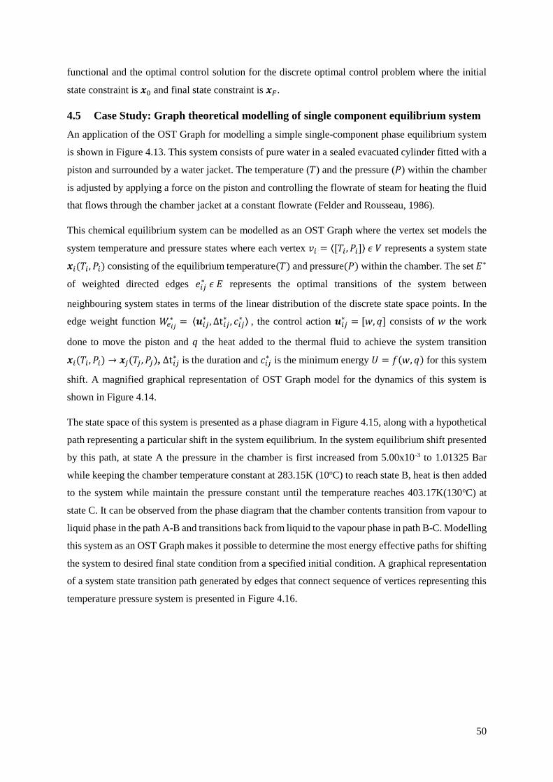
50

functional and the optimal control solution for the discrete optimal control problem where the initial

state constraint is 𝒙0 and final state constraint is 𝒙𝐹.

4.5 Case Study: Graph theoretical modelling of single component equilibrium system

An application of the OST Graph for modelling a simple single-component phase equilibrium system

is shown in Figure 4.13. This system consists of pure water in a sealed evacuated cylinder fitted with a

piston and surrounded by a water jacket. The temperature (𝑇) and the pressure (𝑃) within the chamber

is adjusted by applying a force on the piston and controlling the flowrate of steam for heating the fluid

that flows through the chamber jacket at a constant flowrate (Felder and Rousseau, 1986).

This chemical equilibrium system can be modelled as an OST Graph where the vertex set models the

system temperature and pressure states where each vertex 𝑣𝑖 = ⟨[𝑇𝑖, 𝑃𝑖]⟩ 𝜖 𝑉 represents a system state

𝒙𝑖(𝑇𝑖 , 𝑃𝑖) consisting of the equilibrium temperature(𝑇) and pressure(𝑃) within the chamber. The set 𝐸∗

of weighted directed edges 𝑒𝑖𝑗∗ 𝜖 𝐸 represents the optimal transitions of the system between

neighbouring system states in terms of the linear distribution of the discrete state space points. In the

edge weight function 𝑊𝑒𝑖𝑗∗ = ⟨𝒖𝑖𝑗

∗ , Δt𝑖𝑗∗ , 𝑐𝑖𝑗

∗ ⟩ , the control action 𝒖𝑖𝑗∗ = [𝑤, 𝑞] consists of 𝑤 the work

done to move the piston and 𝑞 the heat added to the thermal fluid to achieve the system transition

𝒙𝑖(𝑇𝑖 , 𝑃𝑖) → 𝒙𝑗(𝑇𝑗, 𝑃𝑗), Δt𝑖𝑗∗ is the duration and 𝑐𝑖𝑗

∗ is the minimum energy 𝑈 = 𝑓(𝑤, 𝑞) for this system

shift. A magnified graphical representation of OST Graph model for the dynamics of this system is

shown in Figure 4.14.

The state space of this system is presented as a phase diagram in Figure 4.15, along with a hypothetical

path representing a particular shift in the system equilibrium. In the system equilibrium shift presented

by this path, at state A the pressure in the chamber is first increased from 5.00x10-3 to 1.01325 Bar

while keeping the chamber temperature constant at 283.15K (10oC) to reach state B, heat is then added

to the system while maintain the pressure constant until the temperature reaches 403.17K(130oC) at

state C. It can be observed from the phase diagram that the chamber contents transition from vapour to

liquid phase in the path A-B and transitions back from liquid to the vapour phase in path B-C. Modelling

this system as an OST Graph makes it possible to determine the most energy effective paths for shifting

the system to desired final state condition from a specified initial condition. A graphical representation

of a system state transition path generated by edges that connect sequence of vertices representing this

temperature pressure system is presented in Figure 4.16.

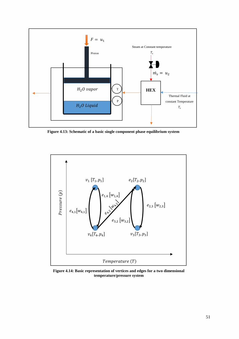
51

𝑣1 [𝑇1, 𝑝1]

𝑣4[𝑇4, 𝑝4]

𝑒2[𝑇2, 𝑝2]

𝑣3[𝑇3, 𝑝3]

𝑇𝑒𝑚𝑝𝑒𝑟𝑎𝑡𝑢𝑟𝑒 (𝑇)

𝑃𝑟𝑒

𝑠𝑠𝑢

𝑟𝑒 (

𝑝)

𝑒4,1[𝑤4,1]

𝑒1,4 [𝑤1,4]

𝑒2,3 [𝑤2,3]

𝑒3,2 [𝑤3,2]

𝑚𝑠ሶ = 𝑢2

𝐻2𝑂 𝑣𝑎𝑝𝑜𝑟

𝐻2𝑂 𝐿𝑖𝑞𝑢𝑖𝑑

HEX

𝐹 = 𝑢1

T

P

Steam at Constant temperature

𝑇𝑠

Thermal Fluid at

constant Temperature

𝑇𝑠

Piston

Figure 4.13: Schematic of a basic single component phase equilibrium system

Figure 4.14: Basic representation of vertices and edges for a two dimensional

temperature/pressure system

52

Figure 4.15: Phase diagram representing the single component H2O system state space indicating a

hypothetical path through from initial state A to final state C

Figure 4.16: Graphical representation of an arbitrary system state transition path through a

temperature, pressure system

𝑤2,3

𝑤5,6 𝑣2 𝑣3

𝑣4

𝑣5

𝑣6

𝑣7

𝑃𝑟𝑒

𝑠𝑠𝑢

𝑟𝑒 (

𝑃)

𝑇𝑒𝑚𝑝𝑒𝑟𝑎𝑡𝑢𝑟𝑒 (𝑇)

State vertex 𝑣𝑖[𝑇𝑖, 𝑃𝑖]

Optimal Path

Legend

Edge 𝑒𝑖𝑗∗

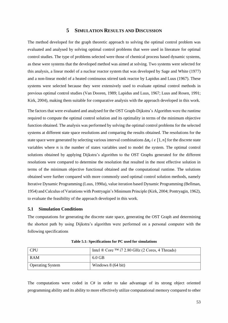
53

5 SIMULATION RESULTS AND DISCUSSION

The method developed for the graph theoretic approach to solving the optimal control problem was

evaluated and analysed by solving optimal control problems that were used in literature for optimal

control studies. The type of problems selected were those of chemical process based dynamic systems,

as these were systems that the developed method was aimed at solving. Two systems were selected for

this analysis, a linear model of a nuclear reactor system that was developed by Sage and White (1977)

and a non-linear model of a heated continuous stirred tank reactor by Lapidus and Luus (1967). These

systems were selected because they were extensively used to evaluate optimal control methods in

previous optimal control studies (Van Dooren, 1989; Lapidus and Luus, 1967; Luus and Rosen, 1991;

Kirk, 2004), making them suitable for comparative analysis with the approach developed in this work.

The factors that were evaluated and analysed for the OST Graph-Dijkstra’s Algorithm were the runtime

required to compute the optimal control solution and its optimality in terms of the minimum objective

function obtained. The analysis was performed by solving the optimal control problems for the selected

systems at different state space resolutions and comparing the results obtained. The resolutions for the

state space were generated by selecting various interval combinations Δ𝒙𝒊 𝑖 𝜖 [1, 𝑛] for the discrete state

variables where 𝑛 is the number of states variables used to model the system. The optimal control

solutions obtained by applying Dijkstra’s algorithm to the OST Graphs generated for the different

resolutions were compared to determine the resolution that resulted in the most effective solution in

terms of the minimum objective functional obtained and the computational runtime. The solutions

obtained were further compared with more commonly used optimal control solution methods, namely

Iterative Dynamic Programming (Luus, 1990a), value iteration based Dynamic Programming (Bellman,

1954) and Calculus of Variations with Pontryagin’s Minimum Principle (Kirk, 2004; Pontryagin, 1962),

to evaluate the feasibility of the approach developed in this work.

5.1 Simulation Conditions

The computations for generating the discrete state space, generating the OST Graph and determining

the shortest path by using Dijkstra’s algorithm were performed on a personal computer with the

following specifications

Table 5.1: Specifications for PC used for simulations

CPU Intel ® Core ™ i7 2.80 GHz (2 Cores, 4 Threads)

RAM 6.0 GB

Operating System Windows 8 (64 bit)

The computations were coded in C# in order to take advantage of its strong object oriented

programming ability and its ability to more effectively utilize computational memory compared to other

54

high level programming languages. The simulations were coded to run on a single processor thread and

standard computational conditions were maintained for all the simulations by ensuring that each

simulation was the only running application in the process stack beside the general background

processes of the operating system. The operating system background processes were also monitored

during the course of each simulation to ensure that no CPU/RAM intensive operating system based

processes interfered with the execution of the computations. The simulation for each resolution was

performed 3 times and the average computation time was recorded.

5.2 Optimal Control of a Linear Nuclear Reactor System

The linear model of a nuclear reactor system developed by Sage and White (1977) was initially used to

evaluate the performance of the OST Graph-Dijksra’s Algorithm approach. This system was used by

Van Dooren (1989) in order to evaluate a Chebychev technique and also used by Luus and Rosen (1991)

to evaluate the Iterative Dynamic Programming (IDP) approach. The optimal control problem for the

nuclear reactor system included the following set of differential equations

where 𝑥1 and 𝑥2 are the state variables for the neutron density and precursor nuclide concentration

respectively, and the control variable 𝑢 is the system’s reactivity. The objective functional to be

minimised is defined by

which a function of the system’s reactivity 𝑢. The general aim of the control problem is to shift the

conditions in the nuclear reactor system from an initial state to a desired final state while minimizing

its reactivity in order to ensure safe operation.

5.2.1 Modelling the dynamic system as an optimal state transition graph

In order to model the dynamics of the nuclear reactor system as an OST Graph, Eq.(5.1) and Eq.(5.2)

were discretized using forward difference discretization and represented in terms of a typical state

transition 𝒙𝑖 → 𝒙𝑗, resulting in the following set of finite difference equations

𝑑𝑥1

𝑑𝑡= 1000(𝑢 − 0.0064)𝑥1 + 0.1𝑥2 (5.1)

𝑑𝑥2

𝑑𝑡= 6.4𝑥1 − 0.1𝑥2 (5.2)

𝐽 = 0.5 ∫ 𝑢2𝑑𝑡𝑡𝑓

0

(5.3)

𝑥𝑗,1 − 𝑥𝑖,1

Δ𝑡𝑖𝑗= 1000(𝑢𝑖𝑗 − 0.0064)𝑥𝑗,1 + 0.1𝑥𝑗,2

(5.4)

55

The objective functional in Eq.(5.3) was also discretized to determine the state transition cost which

was expressed as

As this is a Type B problem (4.4.4), with 𝒙𝑖 and 𝒙𝑗 being known, the following expressions of the

optimal state transition control 𝑢𝑖𝑗∗ and optimal state transition time Δ𝑡𝑖𝑗

∗ in terms of 𝒙𝑖 and 𝒙𝑗 were

determined by manipulating finite differential equations Eq.(5.4) and Eq.(5.5)

where Eq.(5.7) was determined by taking the reciprocal of Eq.(5.5) and Eq.(5.6), and Eq.(5.8) by

changing the subject of the formula in Eq.(5.6). The optimal state transition cost c𝑖𝑗∗ for the state

transitions was expressed as

The OST Graph for this system was generated using the procedure outlined in 4.4. The graph was

defined as

where the vertices in vertex set 𝑉 and the edge weight function 𝑊∗ for the edges 𝑒𝑖𝑗∗ 𝜖 𝐸∗ were expressed

as

𝑣𝑖 = [𝑥1,𝑖, 𝑥2,𝑖] 𝜖 𝑉 (5.11) and 𝑊𝑒𝑖𝑗∗ = ⟨𝑢𝑖𝑗

∗ , Δt𝑖𝑗∗ , 𝑐𝑖𝑗

∗ ⟩, 𝑒𝑖𝑗∗ 𝜖 𝐸∗ (5.12)

The vertex set 𝑉 modelled a two dimensional state space of points which was developed by an upper

and lower bound for the for the state variables and respective interval steps Δ𝑥𝑖, these were then

represented as vertices using the expression in Eq.(5.11). The following constraints were used to

generate the state space and edge weights for the OST Graph

𝑥𝑗,2 − 𝑥𝑖,2

Δ𝑡𝑖𝑗= 6.4𝑥𝑗,1 − 0.1𝑥𝑗,2 (5.5)

𝑐𝑖𝑗 = 0.5 𝑢𝑖𝑗2Δ𝑡𝑖𝑗 (5.6)

𝑢𝑖𝑗∗ =

𝑥𝑗,1 − 𝑥𝑖,1

𝑥𝑗,2 − 𝑥𝑖,2(6.4𝑥𝑗,1 − 0.1𝑥𝑗,2) − 0.1𝑥𝑗,2

1000𝑥𝑗,1+ 0.0064

(5.7)

Δ𝑡𝑖𝑗∗ =

6.4𝑥𝑗,1 − 0.1𝑥𝑗,2

𝑥𝑗,2 − 𝑥𝑖,2 (5.8)

𝑐𝑖𝑗∗ = 0.5𝑢𝑖𝑗

∗ 2Δ𝑡𝑖𝑗

∗ (5.9)

𝐺∗ = (𝑉, 𝐸∗, 𝑊∗) (5.10)

56

The state transitions that resulted in system states and edge weights that are not within these boundaries

are classified as inadmissible and their respective edges are omitted from 𝐸∗.

5.2.2 Analysis of the computational performance for generating the OST Graph and applying

Dikstra’s algorithm

An analysis was first performed on the computational runtime and optimality for the solutions obtained

by the OST Graph-Dijkstra’s Algorithm method at different discrete state space resolutions. This was

to evaluate whether it was computationally feasible to pursue such an approach in terms of the

computational runtime required to obtain a solution and the quality of the solution. The optimal control

problem for which the analysis was performed was of shifting the nuclear reactor system from an initial

state 𝒙𝟎 = [0.5, 32.0] to final state 𝒙𝑭 = [2.7 , 36.5] while ensuring the constraints in Eq.(5.13)-(5.16)

were satisfied. OST Graphs for various discrete state space resolutions were generated and Dijkstra’s

Algorithm was applied to determine the cost of the shortest path from 𝑣0 = ⟨𝒙𝟎⟩ to 𝑣𝐹 = ⟨𝒙𝑭⟩, an

equivalent to the minimum objective functional of the optimal trajectory from 𝒙𝟎 to 𝒙𝑭 in the discrete

state space.

The results from Table 5.2 showed that the number of vertices together with the number of edges of the

generated graphs increased as the values for the [Δ𝑥1, Δ𝑥2] increments were decreased. This was

expected as a finer resolution resulted in more points in the discrete state space and a larger number of

state transitions that needed to be modelled by the graph. The number of generated edges though was

not proportional to the number of vertices, as was observed when comparing R6 and R8. This was due

to edges with weights that do not satisfy the optimal problem constraints in Eq.(5.15)-(5.16) being

omitted from the edge set when the OST Graphs were generated. The variations in the number of graph

edges in proportion to the vertices for the generated graphs were observed in the average vertex degree

for the different graphs. The average vertex degree is an indication of the average number of edges

entering and leaving the vertices in the graph. Ideally, this measure is constant and independent of the

resolutions used for the generated graphs, however, some of the graphs were observed to have lower

average vertex degrees. This is due to the state transition edges that were omitted from the graph edge

set for not satisfying the constraints for the transitions at the different resolutions. The average vertex

degree is therefore an indirect indicator of graph connectivity and how well the optimal state transitions

in discrete state space satisfied the state transition constraints. It was also observed from Table 5.2 that

the average vertex degree for the generated graphs were dependent on the Δ𝑥1

Δ𝑥2 ratio of the discrete state

0.5 ≤ 𝑥1 ≤ 5.0 (5.13)

32.0 ≤ 𝑥2 ≤ 37.0 (5.14)

Δ𝑡𝑖𝑗∗ ≥ 0 (5.15)

0 ≤ 𝑢𝑖𝑗∗ ≤ 0.02 (5.16)

57

space resolutions where a lower Δ𝑥1

Δ𝑥2 ratio resulted in a higher average vertex degree. This indicated that

the successfully representing the discrete dynamic system state space as an OST Graph was dependent

on the selected Δ𝒙𝒊 increments that were selected for the resolution.

OST Graphs for all the selected resolutions were successfully generated except for R9, which was not

completely generated because the computational memory required to generate the graph elements and

to optimize the edge weights, exceeded the available PC RAM. The results in Table 5.2 show that the

memory required to store the OST Graph increased accordingly with the number of edges contained in

the edge set of the graph. The values for “Memory required to store OST Graph” stipulated in this table

are of the memory needed to ‘store’ the OST Graph, excluding the memory that was required to perform

the necessary computations for generating the graph. However, they serve as a good indicator of how

significantly the memory required to store the OST Graph increased the as the state space resolution

became finer.

Table 5.2: Characteristics of OST Graphs generated at different state space resolutions

Resolution

No. 𝚫𝒙𝟏 𝚫𝒙𝟐

𝚫𝒙𝟏

𝚫𝒙𝟐

Number of

Vertices

Number

of

Edges

Average

Vertex

Degree

Memory

Required

to Store

OST

Graph

(KB)

R1 0.1 0.1 1 2 346 6 261 5.34 455

R2 0.1 0.01 10 23 046 45 000 3.91 3 508

R3 0.1 0.001 100 23 0046 450 000 3.91 36 384

R4 0.01 0.1 0.1 23 001 66 925 5.82 5 609

R5 0.01 0.01 1 225 951 510 194 4.52 41 358

R6 0.01 0.001 10 2 255 451 4 482 902 3.98 381 475

R7 0.001 0.1 0.01 229 551 669 045 5.83 52 601

R8 0.001 0.01 0.1 2 255 001 6 691 525 5.93 549 682

R9 0.001 0.001 1 22 509 501 - - -

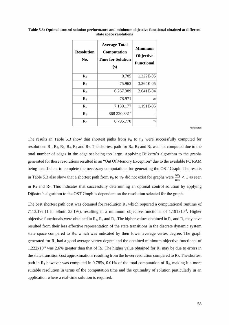
58

Table 5.3: Optimal control solution performance and minimum objective functional obtained at different

state space resolutions

Resolution

No.

Average Total

Computation

Time for Solution

(s)

Minimum

Objective

Functional

R1 0.785 1.222E-05

R2 75.963 3.364E-05

R3 6 267.389 2.641E-04

R4 78.971 ∞

R5 7 139.177 1.191E-05

R6 868 220.831* -

R7 6 795.770 ∞

*estimated

The results in Table 5.3 show that shortest paths from 𝑣0 to 𝑣𝐹 were successfully computed for

resolutions R1, R2, R3, R4, R5 and R7. The shortest path for R6, R8 and R9 was not computed due to the

total number of edges in the edge set being too large. Applying Dijkstra’s algorithm to the graphs

generated for these resolutions resulted in an “Out Of Memory Exception” due to the available PC RAM

being insufficient to complete the necessary computations for generating the OST Graph. The results

in Table 5.3 also show that a shortest path from 𝑣0 to 𝑣𝐹 did not exist for graphs were Δ𝑥1

Δ𝑥2< 1 as seen

in R4 and R7. This indicates that successfully determining an optimal control solution by applying

Dijkstra’s algorithm to the OST Graph is dependent on the resolution selected for the graph.

The best shortest path cost was obtained for resolution R5 which required a computational runtime of

7113.19s (1 hr 58min 33.19s), resulting in a minimum objective functional of 1.191x10-5. Higher

objective functionals were obtained in R1, R2 and R3. The higher values obtained in R2 and R3 may have

resulted from their less effective representation of the state transitions in the discrete dynamic system

state space compared to R5, which was indicated by their lower average vertex degree. The graph

generated for R1 had a good average vertex degree and the obtained minimum objective functional of

1.222x10-5 was 2.6% greater than that of R5. The higher value obtained for R1 may be due to errors in

the state transition cost approximations resulting from the lower resolution compared to R5. The shortest

path in R1 however was computed in 0.785s, 0.01% of the total computation of R5, making it a more

suitable resolution in terms of the computation time and the optimality of solution particularly in an

application where a real-time solution is required.

59

5.2.3 Analysis of optimal control solutions determined by Dijksra’s Algorithm

The state space trajectory of the optimal control solution determined by applying Dijkstra’s algorithm

to R5 was plotted with trajectories that were obtained by applying the Depth-First Search (Alternate

Path A) and Best-First Search (Alternate path B) graph search algorithms to determine the shortest path

from 𝑣0 = ⟨𝒙𝟎⟩ to 𝑣𝐹 = ⟨𝒙𝑭⟩ in R5. All the trajectories were plotted on a Poincare plot with an optimal

path vector field that indicated the general optimal path direction across the system state space as shown

in Figure 5.1. This field represents a greedy strategy where each vector represents the magnitude and

direction of the most optimal transition from a vertex. The vectors were generated at each state point

on a state space grid, at state point increments Δ𝑥1= Δ𝑥2= 0.1. Increments of 0.1 were selected instead

of 0.01 because the vectors for 0.01 increments were not sufficiently visible for analysis. The total cost

(objective functional) of each path is equivalent to the line integral along the path is taken across the

vector field.

It is observed from this plot that the path generated by Dijkstra’s algorithm initially followed a direction

that favoured the direction indicated by the optimal transition direction vectors, however it was

observed that it later deviated from the direction indicated by these vectors and tended towards the

direction of the final state. The Depth-First Search (DFS) algorithm determineed a more direct shortest

path from the initial state to the final state but the total path cost was greater than that of the shortest

path determined by Dijkstra’s algorithm. This was expected as majority of the DFS path was in a

direction that opposed the direction of the optimal transition vectors. The Best-First Search (BFSH)

algorithm is a greedy approach that always selects the adjacent vertex with the lowest state transition

cost at each stage of the path search. It is observed in Figure 5.1 that the BFSH path was initially along

the direction indicated by the optimal transition vectors, this made sense from a greedy search

perspective however this later resulted in a much greater cost being incurred to reach the specified final

system state at a later stage of the search. In this graph, it was therefore more effective for the shortest

path to deviate from the direction of the optimal transition vectors at an earlier stage in order to obtain

a globally optimal shortest path cost. Dijkstra’s algorithm was able to determine such a path because it

is an algorithm that is greedy at a global basis where the vertex with the lowest overall path cost is

selected at each stage of the search, which resulted in a globally optimal solution. Algorithms that are

greedy on a local basis (like BFSH) generally do not result in a globally optimal solution. It was further

concluded from this analysis that even though the generated graph is an OST Graph the optimality of a

path between two vertices, and hence the state space trajectory between two states in the discrete state

space, is dependent on the ability of the applied algorithm to determine the globally optimal solution.

A three dimensional view of these trajectories on a surface plot representing the optimal cost to state is

presented in Figure 5.2.

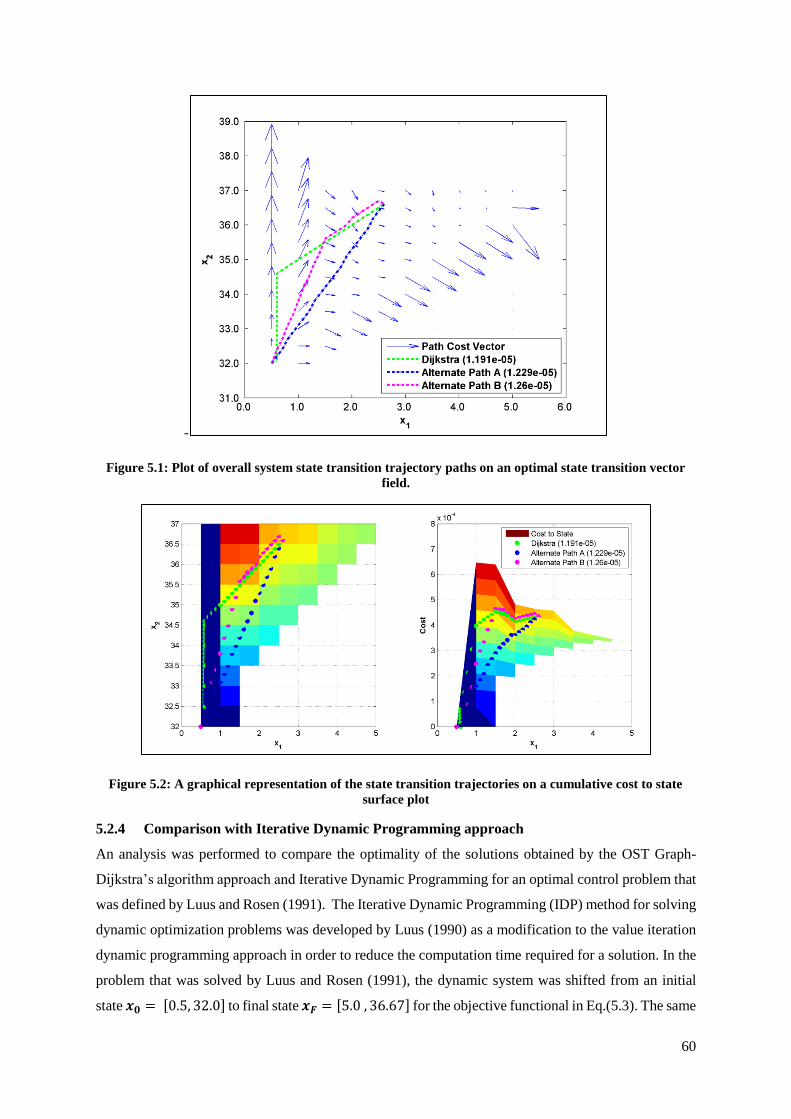
60

-

Figure 5.1: Plot of overall system state transition trajectory paths on an optimal state transition vector

field.

Figure 5.2: A graphical representation of the state transition trajectories on a cumulative cost to state

surface plot

5.2.4 Comparison with Iterative Dynamic Programming approach

An analysis was performed to compare the optimality of the solutions obtained by the OST Graph-

Dijkstra’s algorithm approach and Iterative Dynamic Programming for an optimal control problem that

was defined by Luus and Rosen (1991). The Iterative Dynamic Programming (IDP) method for solving

dynamic optimization problems was developed by Luus (1990) as a modification to the value iteration

dynamic programming approach in order to reduce the computation time required for a solution. In the

problem that was solved by Luus and Rosen (1991), the dynamic system was shifted from an initial

state 𝒙𝟎 = [0.5, 32.0] to final state 𝒙𝑭 = [5.0 , 36.67] for the objective functional in Eq.(5.3). The same

61

problem was solved by applying the OST Graph-Dijkstra’s algorithm approach to compare the solution

that would be obtained with that which was published by Luus and Rosen (1991).

The OST Graph-Dijkstra’s algorithm solution for this problem was determined by applying Dijkstra’s

algorithm to compute the shortest path from 𝑣0 = ⟨𝒙𝟎⟩ to 𝑣𝐹 = ⟨𝒙𝑭⟩ in the OST Graph that was

generated for discrete state space resolution R5, the resolution which provided the best optimal control

result was for the analysis in 5.1.2. The state space trajectory and optimal control from the computed

shortest path was plotted together with the state trajectory and optimal control solution published by

Luus and Rosen (1991) in Figure 5.3 and Figure 5.4 respectively. The minimum value for the objective

functional obtained by Dijkstra’s algorithm was 1.766x10-5, 0.39% lower than the value of 1.773x10-5

that was obtained by IDP. The state space paths in Figure 5.3 show that the state space trajectories for

the two solution methods were similar. The OST Graph-Dijkstra’s algorithm approach solution

trajectory showed to have taken a slight deviation from the IDP solution trajectory, which resulted in

the lower minimum objective functional cost. The optimal control plots in Figure 5.4 show that the

optimal control determined by the OST Graph-Dijkstra’s algorithm approach had resulted in the system

taking a greater time to shift from 𝒙𝟎 to 𝒙𝑭 compared to the optimal control that was determined by

IDP. Overall, these results clearly indicated that the approach developed in this work was able to

determine an optimal control solution that were comparable to IDP.

Figure 5.3: State space trajectories for the optimal control solutions obtained by the OST Graph-

Dijkstra’s Algorithm and Iterative Dynamic Programming methods

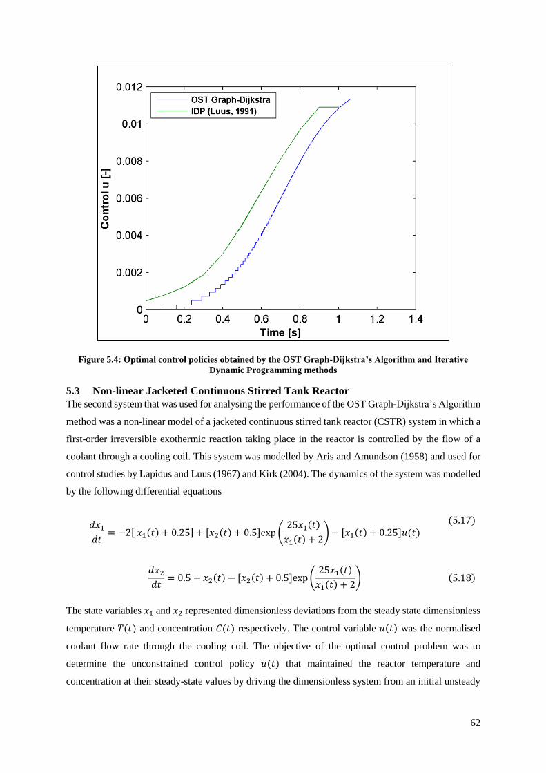
62

Figure 5.4: Optimal control policies obtained by the OST Graph-Dijkstra’s Algorithm and Iterative

Dynamic Programming methods

5.3 Non-linear Jacketed Continuous Stirred Tank Reactor

The second system that was used for analysing the performance of the OST Graph-Dijkstra’s Algorithm

method was a non-linear model of a jacketed continuous stirred tank reactor (CSTR) system in which a

first-order irreversible exothermic reaction taking place in the reactor is controlled by the flow of a

coolant through a cooling coil. This system was modelled by Aris and Amundson (1958) and used for

control studies by Lapidus and Luus (1967) and Kirk (2004). The dynamics of the system was modelled

by the following differential equations

The state variables 𝑥1 and 𝑥2 represented dimensionless deviations from the steady state dimensionless

temperature 𝑇(𝑡) and concentration 𝐶(𝑡) respectively. The control variable 𝑢(𝑡) was the normalised

coolant flow rate through the cooling coil. The objective of the optimal control problem was to

determine the unconstrained control policy 𝑢(𝑡) that maintained the reactor temperature and

concentration at their steady-state values by driving the dimensionless system from an initial unsteady

𝑑𝑥1

𝑑𝑡= −2[ 𝑥1(𝑡) + 0.25] + [𝑥2(𝑡) + 0.5]exp (

25𝑥1(𝑡)

𝑥1(𝑡) + 2) − [𝑥1(𝑡) + 0.25]𝑢(𝑡)

(5.17)

𝑑𝑥2

𝑑𝑡= 0.5 − 𝑥2(𝑡) − [𝑥2(𝑡) + 0.5]exp (

25𝑥1(𝑡)

𝑥1(𝑡) + 2) (5.18)

63

state towards the origin (steady state) without expending a large amount of coolant (control effort). The

objective functional to be minimised was expressed as

where the control input weight factor of R= 0.1 was selected. Minimization of the objective functional

in Eq.(5.19) indicated that the objective was to maintain the temperature and concentration of reactant

in the reactor close to their steady-state values while minimizing the amount of cooling water needed

to do so. This optimal control problem is known as a fixed-final state, free final time problem. An

investigation that was performed by Luus and Cormack (1972) on the characteristics of this system

showed that there existed multiple locally optimal solutions when optimal control problems for this

system were solved by the calculus of variations, making it difficult for a globally optimal solution to

be determined.

5.3.1 Modelling the dynamic system as an optimal state transition graph

The set of forward difference equations, derived from Eq.(5.17) and Eq.(5.18), that were used to

represent a state transition 𝒙𝑖 → 𝒙𝑗 of the CSTR system were expressed as

The discrete objective functional for the state transition cost of the transition 𝒙𝑖 → 𝒙𝑗 derived from

Eq.(5.19) was expressed as

This was a Type B system (4.4.4) where 𝒙𝑖 and 𝒙𝑗 are known. The optimal state transition control 𝑢𝑖𝑗∗

and optimal state transition time Δ𝑡𝑖𝑗∗ were determined in terms of the known initial and final states 𝒙𝑖

and 𝒙𝑗 by manipulating of the discrete state transition equations Eq.(5.20) and Eq.(5.21) which resulted

in the following expression for the state transition control

𝐽 = ∫ (𝑥12(𝑡) + 𝑥2

2(𝑡) + 𝑅𝑢2) 𝑑𝑡𝑡𝑓

0

(5.19)

𝑥𝑗,1 − 𝑥𝑖,1

Δ𝑡𝑖𝑗= −2( 𝑥𝑗,1 + 0.25) + (𝑥𝑗,2 + 0.5)exp (

25𝑥𝑗,1

𝑥𝑗,1 + 2) − (𝑥𝑗,1 + 0.25)𝑢𝑖𝑗

(5.20)

𝑥𝑗,2 − 𝑥𝑖,2

Δ𝑡𝑖𝑗= 0.5 − 𝑥𝑗,2 − (𝑥𝑗,2 + 0.5)exp (

25𝑥𝑗,1

𝑥𝑗,1 + 2)

(5.21)

𝑐𝑖𝑗 = (𝑥1,𝑖2 + 𝑥2,𝑖

2 + 𝑅 𝑢𝑖𝑗2 )Δ𝑡𝑖𝑗 (5.22)

𝑢𝑖𝑗∗ =

𝐴 − 𝐶𝐷

𝐵 (5.23)

𝐴 = −2( 𝑥𝑗,1 + 0.25) + (𝑥𝑗,2 + 0.5)exp (25𝑥𝑗,1

𝑥𝑗,1 + 2) (5.24)

64

and the following expression for the state transition time

Eq.(5.23) was determined by taking the reciprocal of Eq.(5.20) and Eq.(5.21), and Eq.(5.28) by

changing the subject of the formula in Eq.(5.21). The optimal state transition cost was expressed as

The OST Graph 𝐺∗ = (𝑉, 𝐸∗, 𝑊∗) was generated by the procedure outlined in 4.4 where the vertices in

vertex set 𝑉 and the weights of the edges in 𝐸∗ were expressed as

𝑣𝑖 = [𝑥1,𝑖, 𝑥2,𝑖] 𝜖 𝑉 (5.23) and 𝑊𝑒𝑖𝑗∗ = ⟨𝑢𝑖𝑗

∗ , Δt𝑖𝑗∗ , 𝑐𝑖𝑗

∗ ⟩, 𝑒𝑖𝑗∗ 𝜖 𝐸∗ (5.34)

The following constraints were applied to the generated graph.

5.3.2 Comparison with Calculus of Variations approach

An analysis was performed to compare the optimality of the OST Graph-Dijkstra’s algorithm approach

with the calculus of variations approach to solving the optimal control problem. The optimal control

problem used to compare these two methods involved shifting the stirred tank reactor system from

initial state 𝒙𝟎 = [0.09,0.09] to final state 𝒙𝑭 = [0.001,0.001], a final state that is relatively close to

the steady state operating point.

The Variational Calculus based solution was evaluated by applying the Calculus of Variations to

determine necessary conditions for optimality and solving the resulting set of equations as a Boundary

Value Problem (BVP). The resulting equations were too complex to be solved analytically and were

solved numerically by utilizing the bvp4c MATLAB™ solver, an effective ODE solver dedicated for

boundary value problems. Shampine et al. (2000) is an excellent reference for using bvp4c. The

𝐵 = 𝑥𝑗,1 + 0.25 (5.25)

𝐶 = 0.5 − 𝑥𝑗,2 − (𝑥𝑗,2 + 0.5)exp (25𝑥𝑗,1

𝑥𝑗,1 + 2) (5.26)

𝐷 = 𝑥𝑗,1 − 𝑥𝑖,1

𝑥𝑗,2 − 𝑥𝑖,2 (5.27)

Δ𝑡𝑖𝑗∗ =

𝑥𝑗,2 − 𝑥𝑖,2

0.5 − 𝑥𝑗,2 − (𝑥𝑗,2 + 0.5)exp (25𝑥𝑗,1

𝑥𝑗,1 + 2)

(5.28)

𝑐𝑖𝑗∗ = (𝑥1,𝑖

2 + 𝑥2,𝑖2 + 𝑅 𝑢𝑖𝑗

∗ 2)Δ𝑡𝑖𝑗

∗ (5.22)

−0.10 ≤ 𝑥1 ≤ 0.10 (5.25)

−0.05 ≤ 𝑥2 ≤ 0.10 (5.26)

Δ𝑡𝑖𝑗∗ ≥ 0 (5.27)

0 ≤ 𝑢𝑖𝑗∗ ≤ 7.0 (5.28)

65

necessary conditions for optimality that were determined by applying the calculus of variations resulted

in the following set of equations

where Eq.(5.29) and Eq.(5.30) are known as the costate equations (Kirk, 2004). Rearranging the

algebraic relation in Eq.(5.31) resulted in the following expression

for the control 𝑢 in terms of the state and costates. Substituting Eq.(5.32) into Eq.(5.17) and Eq.(5.29)

resulted in a set of four first-order ordinary differential equations (ODE’s): 𝑑𝑥1

𝑑𝑡,

𝑑𝑥2

𝑑𝑡,

𝑑𝑝1

𝑑𝑡and

𝑑𝑝2

𝑑𝑡. Solving

the BVP for these equations required four boundary conditions. These were expressed as

where 𝑡𝑓 is the final time that represents the duration of the determined optimal control solution. Since

this was a free final time problem, 𝑡𝑓 was also an unknown variable and a fifth boundary condition was

required. The boundary condition for 𝑡𝑓 was expressed as

and was also determined from the necessary conditions of optimality from the calculus of variations

(Kirk,2004). The four ODE’s, five boundary conditions and an initial guess for the solution in the form

of a mesh were provided as the input for the bvp4c method and the solution was determined.

𝑑𝑝1

𝑑𝑡= −2𝑥1(𝑡) + 2𝑝1(𝑡) − 𝑝1(𝑡)(𝑥2(𝑡) + 0.5) (

50𝑥1(𝑡)

(𝑥1(𝑡) + 2)2) exp (25𝑥1(𝑡)

𝑥1(𝑡) + 2)

+ 𝑝1(𝑡)𝑢(𝑡) + 𝑝2(𝑡)(𝑥2(𝑡) + 0.5) (50𝑥1(𝑡)

(𝑥1(𝑡) + 2)2) exp (25𝑥1(𝑡)

𝑥1(𝑡) + 2)

(5.29)

𝑑𝑝2

𝑑𝑡= −2𝑥2(𝑡) − 𝑝1(𝑡) exp (

25𝑥1(𝑡)

𝑥1(𝑡) + 2) + 𝑝2(𝑡) (1 + exp (

25𝑥1(𝑡)

𝑥1(𝑡) + 2)) (5.30)

2𝑅𝑢(𝑡) − 𝑝1(𝑡)(𝑥1(𝑡) + 0.25) = 0 (5.31)

𝑢(𝑡) =𝑝1(𝑡)(𝑥1(𝑡) + 0.25)

2𝑅 (5.32)

𝑥1(0) = 0.09 , 𝑥2(0) = 0.09 , 𝑥1(𝑡𝑓) = 0.001, 𝑥2(𝑡𝑓) = 0.001 (5.33)

𝑥12(𝑡𝑓) + 𝑥2

2(𝑡𝑓) + 𝑅 (𝑝1(𝑡𝑓)(𝑥1(𝑡𝑓) + 0.25)

2𝑅)

2

+ 𝑝1(𝑡𝑓) (−2( 𝑥1(𝑡𝑓) + 0.25) + (𝑥2(𝑡𝑓) + 0.5)exp (25𝑥1(𝑡𝑓)

𝑥1(𝑡𝑓) + 2)

− (𝑥1(𝑡𝑓) + 0.25) (𝑝1(𝑡𝑓)(𝑥1(𝑡𝑓) + 0.25)

2𝑅) )

+ 𝑝2(𝑡𝑓) (0.5 − 𝑥2(𝑡) − (𝑥2(𝑡𝑓) + 0.5)exp (25𝑥1(𝑡𝑓)

𝑥1(𝑡𝑓) + 2)) = 0

(5.34)

66

The OST Graph that was used for the OST Graph-Dijkstra’s Algorithm approach was generated by

selecting the state space intervals Δ𝑥1, Δ𝑥2 = 5 x 10−4, which together with the constraints in

Eq.(5.25)-(5.28) resulted in an OST Graph of 120701 vertices, 357429 edges and an average vertex

degree of 5.92. The high vertex degree indicated that the generated graph provided a good representation

of the system dynamics.

The optimal state space trajectories that were determined by the OST Graph-Dijkstra’s Algorithm

approach and the calculus of variations approach were plotted in Figure 5.5, and their respective optimal

control solutions were plotted in Figure 5.6. The solution determined by the OST Graph-Dijkstra’s

Algorithm approach resulted in a lower minimum objective functional of 𝐽∗= 0.1545 compared to 𝐽∗=

0.1812 which was obtained by the variational calculus approach. The plots of the optimal controls in

Figure 5.6 show that the variational calculus solution resulted an optimal control that allowed for the

final state to be reached at a much shorter duration of 0.2755s compared to the 0.5567s of the OST

Graph-Dijkstra’s Algorithm solution. Integrating the control curves to determine the total normalized

coolant used showed that the solution determined by the OST Graph-Dijkstra’s Algorithm approach

resulted in a lower total coolant utilization of 0.5508 compared to 0.5756 obtained for the variational

calculus approach. These results indicated that there existed a trade-off between the time taken to reach

the final state and the amount of coolant used, where a shorter system transition time resulted in more

coolant being used. In Figure 5.6, the state space trajectory of the solution determined by the OST

Graph-Dijkstra’s Algorithm approach was observed to take on a more direct path from initial the state

to the final state the state space as compared to that which was determined by the calculus of variations

based solution. This resulted in a lower overall path cost due to deviation from steady state as compared

to the variational calculus approach.

It can be concluded from the results obtained in this comparison that the OST Graph-Dijkstra’s

Algorithm approach was able to produce an optimal control solution that was 14.74% more optimal

than the numerically solved Calculus of Variation approach.

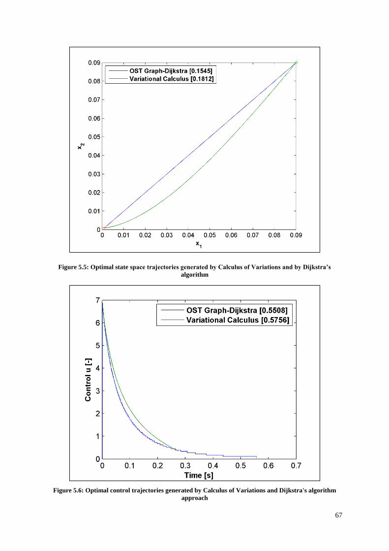
67

Figure 5.5: Optimal state space trajectories generated by Calculus of Variations and by Dijkstra’s

algorithm

Figure 5.6: Optimal control trajectories generated by Calculus of Variations and Dijkstra's algorithm

approach

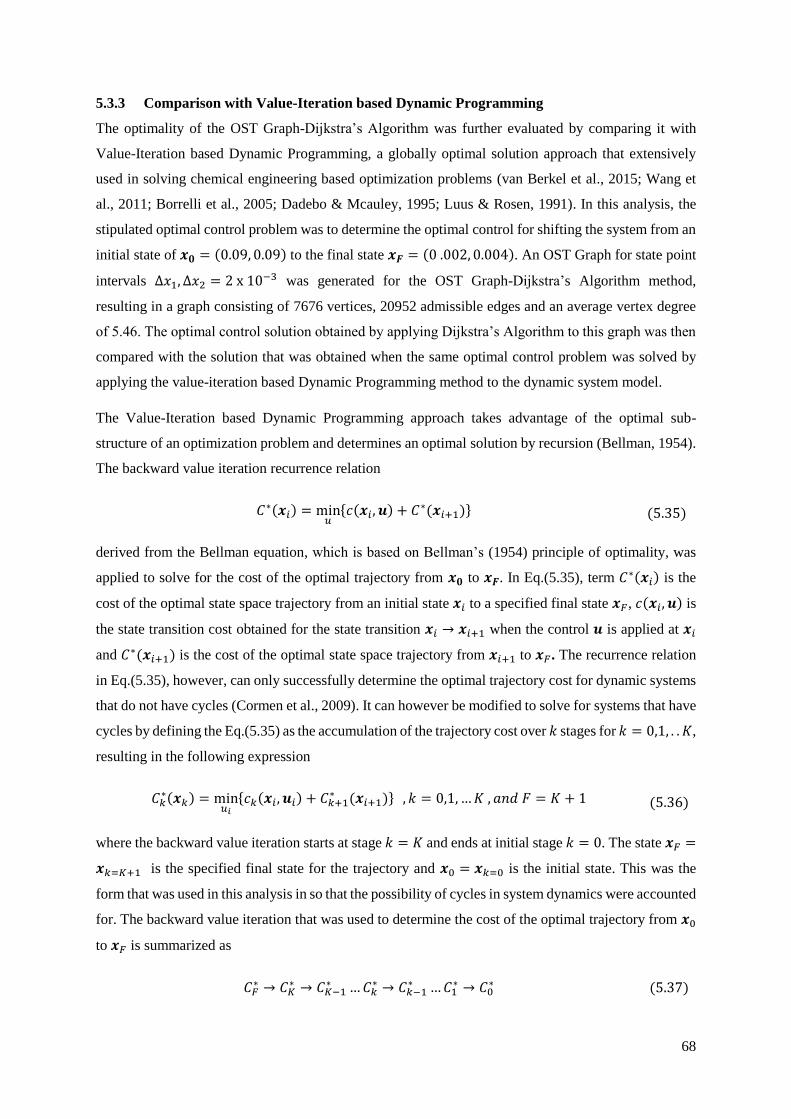
68

5.3.3 Comparison with Value-Iteration based Dynamic Programming

The optimality of the OST Graph-Dijkstra’s Algorithm was further evaluated by comparing it with

Value-Iteration based Dynamic Programming, a globally optimal solution approach that extensively

used in solving chemical engineering based optimization problems (van Berkel et al., 2015; Wang et

al., 2011; Borrelli et al., 2005; Dadebo & Mcauley, 1995; Luus & Rosen, 1991). In this analysis, the

stipulated optimal control problem was to determine the optimal control for shifting the system from an

initial state of 𝒙𝟎 = (0.09, 0.09) to the final state 𝒙𝑭 = (0 .002, 0.004). An OST Graph for state point

intervals Δ𝑥1, Δ𝑥2 = 2 x 10−3 was generated for the OST Graph-Dijkstra’s Algorithm method,

resulting in a graph consisting of 7676 vertices, 20952 admissible edges and an average vertex degree

of 5.46. The optimal control solution obtained by applying Dijkstra’s Algorithm to this graph was then

compared with the solution that was obtained when the same optimal control problem was solved by

applying the value-iteration based Dynamic Programming method to the dynamic system model.

The Value-Iteration based Dynamic Programming approach takes advantage of the optimal sub-

structure of an optimization problem and determines an optimal solution by recursion (Bellman, 1954).

The backward value iteration recurrence relation

derived from the Bellman equation, which is based on Bellman’s (1954) principle of optimality, was

applied to solve for the cost of the optimal trajectory from 𝒙𝟎 to 𝒙𝑭. In Eq.(5.35), term 𝐶∗(𝒙𝑖) is the

cost of the optimal state space trajectory from an initial state 𝒙𝑖 to a specified final state 𝒙𝐹, 𝑐(𝒙𝑖, 𝒖) is

the state transition cost obtained for the state transition 𝒙𝑖 → 𝒙𝑖+1 when the control 𝒖 is applied at 𝒙𝑖

and 𝐶∗(𝒙𝑖+1) is the cost of the optimal state space trajectory from 𝒙𝑖+1 to 𝒙𝐹. The recurrence relation

in Eq.(5.35), however, can only successfully determine the optimal trajectory cost for dynamic systems

that do not have cycles (Cormen et al., 2009). It can however be modified to solve for systems that have

cycles by defining the Eq.(5.35) as the accumulation of the trajectory cost over 𝑘 stages for 𝑘 = 0,1, . . 𝐾,

resulting in the following expression

where the backward value iteration starts at stage 𝑘 = 𝐾 and ends at initial stage 𝑘 = 0. The state 𝒙𝐹 =

𝒙𝑘=𝐾+1 is the specified final state for the trajectory and 𝒙0 = 𝒙𝑘=0 is the initial state. This was the

form that was used in this analysis in so that the possibility of cycles in system dynamics were accounted

for. The backward value iteration that was used to determine the cost of the optimal trajectory from 𝒙0

to 𝒙𝐹 is summarized as

𝐶∗(𝒙𝑖) = min𝑢

{𝑐(𝒙𝑖, 𝒖) + 𝐶∗(𝒙𝑖+1)} (5.35)

𝐶𝑘∗(𝒙𝑘) = min

𝑢𝑖

{𝑐𝑘(𝒙𝑖, 𝒖𝑖) + 𝐶𝑘+1∗ (𝒙𝑖+1)} , 𝑘 = 0,1, … 𝐾 , 𝑎𝑛𝑑 𝐹 = 𝐾 + 1 (5.36)

𝐶𝐹∗ → 𝐶𝐾

∗ → 𝐶𝐾−1∗ … 𝐶𝑘

∗ → 𝐶𝑘−1∗ … 𝐶1

∗ → 𝐶0∗ (5.37)

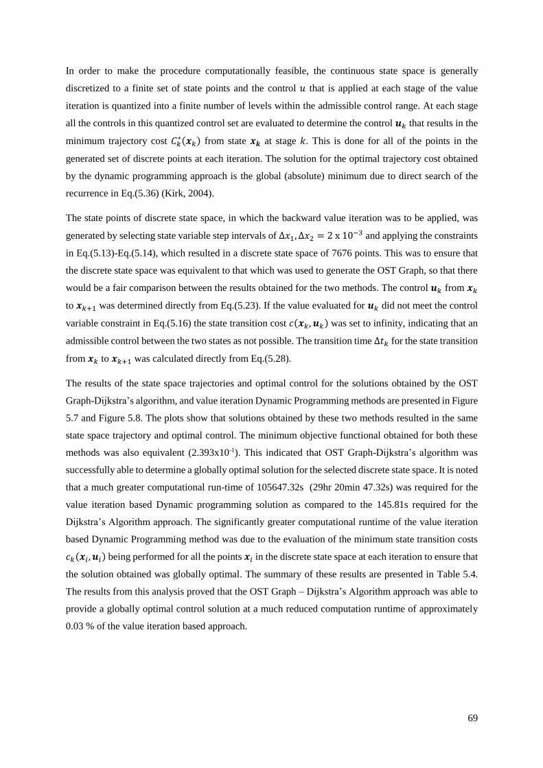
69

In order to make the procedure computationally feasible, the continuous state space is generally

discretized to a finite set of state points and the control 𝑢 that is applied at each stage of the value

iteration is quantized into a finite number of levels within the admissible control range. At each stage

all the controls in this quantized control set are evaluated to determine the control 𝒖𝑘 that results in the

minimum trajectory cost 𝐶𝑘∗(𝒙𝑘) from state 𝒙𝒌 at stage 𝑘. This is done for all of the points in the

generated set of discrete points at each iteration. The solution for the optimal trajectory cost obtained

by the dynamic programming approach is the global (absolute) minimum due to direct search of the

recurrence in Eq.(5.36) (Kirk, 2004).

The state points of discrete state space, in which the backward value iteration was to be applied, was

generated by selecting state variable step intervals of Δ𝑥1, Δ𝑥2 = 2 x 10−3 and applying the constraints

in Eq.(5.13)-Eq.(5.14), which resulted in a discrete state space of 7676 points. This was to ensure that

the discrete state space was equivalent to that which was used to generate the OST Graph, so that there

would be a fair comparison between the results obtained for the two methods. The control 𝒖𝑘 from 𝒙𝑘

to 𝒙𝑘+1 was determined directly from Eq.(5.23). If the value evaluated for 𝒖𝑘 did not meet the control

variable constraint in Eq.(5.16) the state transition cost 𝑐(𝒙𝑘, 𝒖𝑘) was set to infinity, indicating that an

admissible control between the two states as not possible. The transition time Δ𝑡𝑘 for the state transition

from 𝒙𝑘 to 𝒙𝑘+1 was calculated directly from Eq.(5.28).

The results of the state space trajectories and optimal control for the solutions obtained by the OST

Graph-Dijkstra’s algorithm, and value iteration Dynamic Programming methods are presented in Figure

5.7 and Figure 5.8. The plots show that solutions obtained by these two methods resulted in the same

state space trajectory and optimal control. The minimum objective functional obtained for both these

methods was also equivalent (2.393x10-1). This indicated that OST Graph-Dijkstra’s algorithm was

successfully able to determine a globally optimal solution for the selected discrete state space. It is noted

that a much greater computational run-time of 105647.32s (29hr 20min 47.32s) was required for the

value iteration based Dynamic programming solution as compared to the 145.81s required for the

Dijkstra’s Algorithm approach. The significantly greater computational runtime of the value iteration

based Dynamic Programming method was due to the evaluation of the minimum state transition costs

𝑐𝑘(𝒙𝑖, 𝒖𝑖) being performed for all the points 𝒙𝑖 in the discrete state space at each iteration to ensure that

the solution obtained was globally optimal. The summary of these results are presented in Table 5.4.

The results from this analysis proved that the OST Graph – Dijkstra’s Algorithm approach was able to

provide a globally optimal control solution at a much reduced computation runtime of approximately

0.03 % of the value iteration based approach.

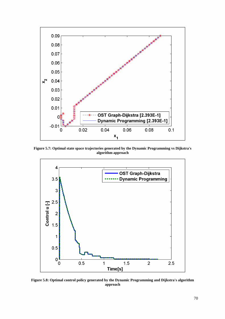
70

Figure 5.7: Optimal state space trajectories generated by the Dynamic Programming vs Dijkstra's

algorithm approach

Figure 5.8: Optimal control policy generated by the Dynamic Programming and Dijkstra's algorithm

approach

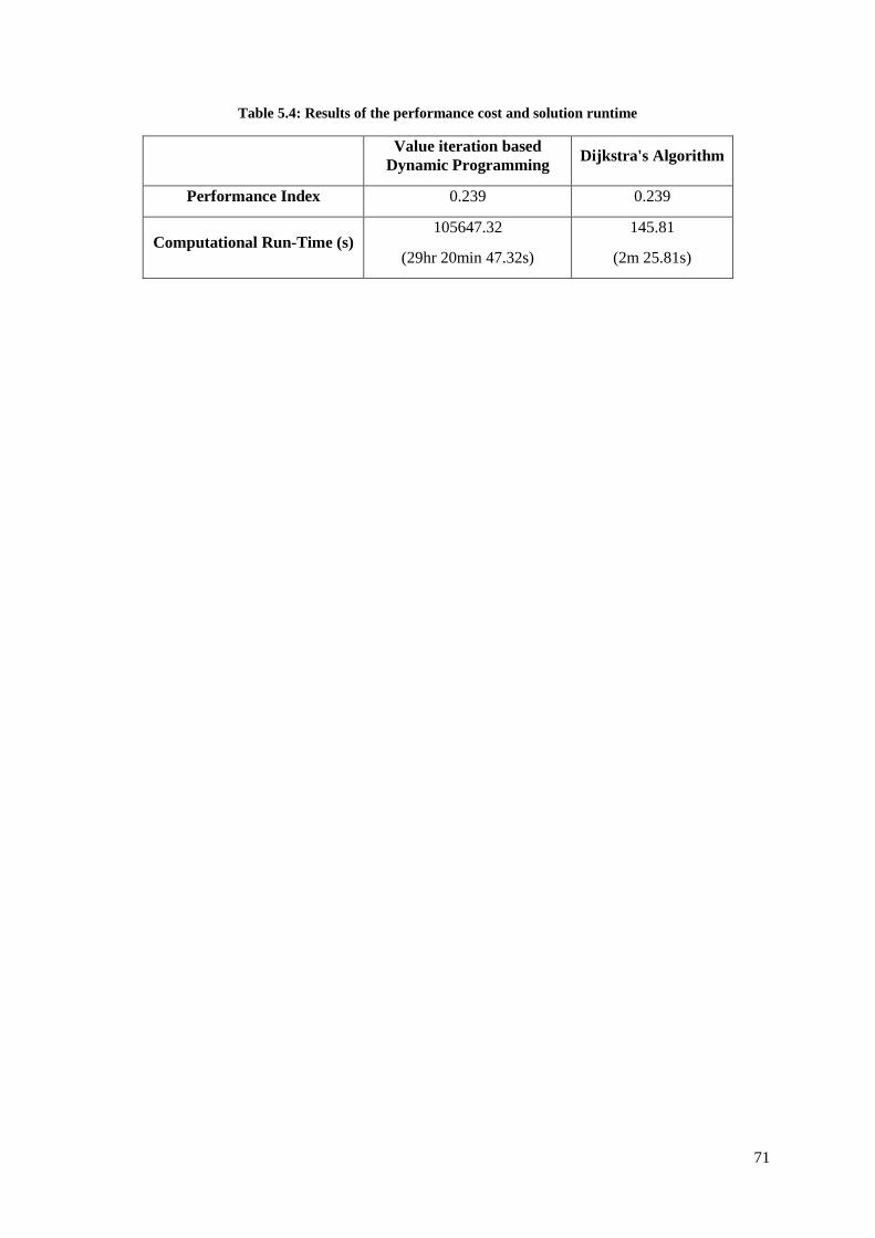
71

Table 5.4: Results of the performance cost and solution runtime

Value iteration based

Dynamic Programming Dijkstra's Algorithm

Performance Index 0.239 0.239

Computational Run-Time (s) 105647.32

(29hr 20min 47.32s)

145.81

(2m 25.81s)

72

6 OST GRAPH RESOLUTION ANALYSIS FOR THE OPTIMAL CONTROL OF A

NON-ADIABATIC BATCH REACTOR SYSTEM

6.1 Batch reactors in industry

In industry, batch processes are generally used in the production of valuable products that result from

complex reaction mechanisms where the reaction pattern is usually controlled by adjustment of the

reaction temperature. These batch reaction processes are common in the pharmaceutical,

microelectronics, food and wine industries (Nagy and Braatz, 2004; Caccavale et al., 2010). As opposed

to continuous reactors that are typically used in large-scale production processes, batch reactors are

frequently used in situations where production rates are relatively low. However, they are also still

widely used in situations where production rates are fairly high due to the kinetic advantages they

exhibit for certain reaction systems. This is often observed in polymerization and fermentation

processes. Batch reactor systems are also known to provide flexibility in production as it is possible for

a single reactor vessel to produce a number of different products under a variety of conditions, making

them very useful in industrial chemical production (Cuthrell and Biegler, 1989; Luyben, 2007).

6.2 The control of batch reactor systems

The control of batch reactor systems is difficult compared to continuous systems because of the

intrinsically unsteady state and nonlinear nature of batch processes, as a result, they require specialized

control systems that can effectively handle process nonlinearity(Luyben, 2007). The control of batch

reactor processes is usually achieved through feedback control where the reactor temperature is initially

ramped up to an optimal reaction temperature and is maintained there until the desired conversion is

achieved (Luus and Okongwu, 1999; Luyben, 2007).

The variations that occur in the process time constants and gains due to the significant changes that

occur in the process variable values make controller tuning a major issue for batch reactor process

control. Controller gain scheduling is an approach that is generally used to resolve this issue, where the

controller tuning constants are changed over time to accommodate the large changes in the process

variable values. Determining how the tuning constants should change, however remains a difficult task

(Cardello and San, 1987; Méndez et al., 2006; Luyben, 2007).

Control optimization has been successfully applied in many batch reactor based processes and interest

in this area of batch process operation continues to grow as batch reactor systems become more complex

(Rippin, 1983; Terwiesch et al., 1994; Bhatia and Biegler, 1997; Luus and Okongwu, 1999; Nagy and

Braatz, 2004). The most frequently used approach for batch reactor optimal control is the open-loop

optimization approach where the optimal control problem is solved for a mathematical model of the

batch reactor system in an offline basis. The optimal control of the determined solution for optimization

is then applied to the reactor system as a series of control inputs over time. Optimal control solution

73

methods that have been successfully used for this approach include Sequential Dynamic Programming

(Logsdon and Biegler, 1993) and Iterative Dynamic Programming (Luus, 1994; Bojkov and Luus,

1996). The highly nonlinear nature of typical batch reactors systems makes it very difficult for optimal

temperature solutions to be obtained by using Pontryagin’s Minimum principle (Wen and Yen, 1977;

Luus, 1978).

The majority of the developments in the area of batch reactor optimal control focus on obtaining the

theoretical optimal temperature profile (or trajectory) where the reactor temperature is taken as the

control variable. Optimal temperature profiles provide information on the reactor operation temperature

ranges and the upper limits for expected reactor yield (Luus and Okongwu, 1999), which is valuable

for reactor design and operation. The obtained temperature profiles, however, cannot be directly applied

as actual control of the reactor, particularly in instances where the profile consists of rapid changes in

temperature.

An alternative approach towards more practical optimal control solutions involves formulating the

optimal control problem where physical elements such as the flow rate of heating and cooling fluids are

used as control variables. This has been successfully applied by Luus and Okongwu (1999) in the

control of elementary reaction based batch reactor systems using the Iterative Dynamic Programming

method. This chapter investigates the practical optimal control of a batch reactor system through the

developed OST Graph- Dijkstra’s Algorithm method. It was also observed in 5.1.2 that the quality of

optimal control solution obtained by the OST Graph-Dijkstra’s algorithm approach is heavily dependent

on resolution of the discrete state space from which the OST Graph is generated.

A more in-depth analysis was performed to determine the relationship between the discrete state space

resolution and the quality of the optimal control solution obtained for the developed batch reactor

system model in order to determine the necessary criteria that a selected discrete state space resolution

must satisfy for good optimal control solution to be obtained.

6.3 Process Description

6.3.1 Reaction Kinetics

An elementary liquid phase, first order reversible exothermic reaction occurring in a batch reactor

system is considered, where the chemical reaction is described by

The first order kinetics for this reversible reactions are

𝐴 ⇌𝑘2

𝑘1 𝐵 Δ𝐻𝑅𝑥𝑛 = −5.5 𝑘𝐽/𝑚𝑜𝑙 (6.1)

𝑟𝐴 = 𝑘1(𝐶𝐴 − 𝐶𝐵/𝐾𝑒) (6.2)

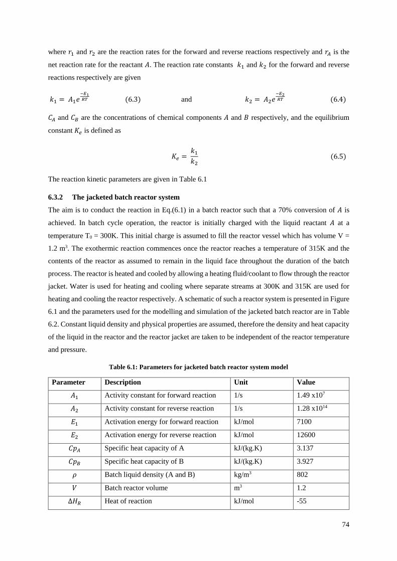
74

where 𝑟1 and 𝑟2 are the reaction rates for the forward and reverse reactions respectively and 𝑟𝐴 is the

net reaction rate for the reactant 𝐴. The reaction rate constants 𝑘1 and 𝑘2 for the forward and reverse

reactions respectively are given

𝑘1 = 𝐴1𝑒−𝐸1𝑅𝑇 (6.3) and 𝑘2 = 𝐴2𝑒

−𝐸2𝑅𝑇 (6.4)

𝐶𝐴 and 𝐶𝐵 are the concentrations of chemical components 𝐴 and 𝐵 respectively, and the equilibrium

constant 𝐾𝑒 is defined as

The reaction kinetic parameters are given in Table 6.1

6.3.2 The jacketed batch reactor system

The aim is to conduct the reaction in Eq.(6.1) in a batch reactor such that a 70% conversion of 𝐴 is

achieved. In batch cycle operation, the reactor is initially charged with the liquid reactant 𝐴 at a

temperature T0 = 300K. This initial charge is assumed to fill the reactor vessel which has volume V =

1.2 m3. The exothermic reaction commences once the reactor reaches a temperature of 315K and the

contents of the reactor as assumed to remain in the liquid face throughout the duration of the batch

process. The reactor is heated and cooled by allowing a heating fluid/coolant to flow through the reactor

jacket. Water is used for heating and cooling where separate streams at 300K and 315K are used for

heating and cooling the reactor respectively. A schematic of such a reactor system is presented in Figure

6.1 and the parameters used for the modelling and simulation of the jacketed batch reactor are in Table

6.2. Constant liquid density and physical properties are assumed, therefore the density and heat capacity

of the liquid in the reactor and the reactor jacket are taken to be independent of the reactor temperature

and pressure.

Table 6.1: Parameters for jacketed batch reactor system model

Parameter Description Unit Value

𝐴1 Activity constant for forward reaction 1/s 1.49 x107

𝐴2 Activity constant for reverse reaction 1/s 1.28 x1014

𝐸1 Activation energy for forward reaction kJ/mol 7100

𝐸2 Activation energy for reverse reaction kJ/mol 12600

𝐶𝑝𝐴 Specific heat capacity of A kJ/(kg.K) 3.137

𝐶𝑝𝐵 Specific heat capacity of B kJ/(kg.K) 3.927

𝜌 Batch liquid density (A and B) kg/m3 802

𝑉 Batch reactor volume m3 1.2

Δ𝐻𝑅 Heat of reaction kJ/mol -55

𝐾𝑒 = 𝑘1

𝑘2 (6.5)

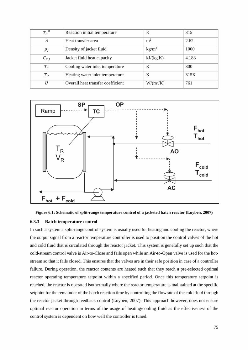
75

𝑇𝑅𝑜 Reaction initial temperature K 315

𝐴 Heat transfer area m2 2.62

𝜌𝐽 Density of jacket fluid kg/m3 1000

𝐶𝑃,𝐽 Jacket fluid heat capacity kJ/(kg.K) 4.183

𝑇𝐶 Cooling water inlet temperature K 300

𝑇𝐻 Heating water inlet temperature K 315K

𝑈 Overall heat transfer coefficient W/(m2/K) 761

Figure 6.1: Schematic of split-range temperature control of a jacketed batch reactor (Luyben, 2007)

6.3.3 Batch temperature control

In such a system a split-range control system is usually used for heating and cooling the reactor, where

the output signal from a reactor temperature controller is used to position the control valves of the hot

and cold fluid that is circulated through the reactor jacket. This system is generally set up such that the

cold-stream control valve is Air-to-Close and fails open while an Air-to-Open valve is used for the hot-

stream so that it fails closed. This ensures that the valves are in their safe position in case of a controller

failure. During operation, the reactor contents are heated such that they reach a pre-selected optimal

reactor operating temperature setpoint within a specified period. Once this temperature setpoint is

reached, the reactor is operated isothermally where the reactor temperature is maintained at the specific

setpoint for the remainder of the batch reaction time by controlling the flowrate of the cold fluid through

the reactor jacket through feedback control (Luyben, 2007). This approach however, does not ensure

optimal reactor operation in terms of the usage of heating/cooling fluid as the effectiveness of the

control system is dependent on how well the controller is tuned.

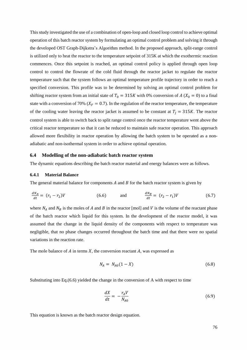
76

This study investigated the use of a combination of open-loop and closed loop control to achieve optimal

operation of this batch reactor system by formulating an optimal control problem and solving it through

the developed OST Graph-Dijkstra’s Algorithm method. In the proposed approach, split-range control

is utilized only to heat the reactor to the temperature setpoint of 315K at which the exothermic reaction

commences. Once this setpoint is reached, an optimal control policy is applied through open loop

control to control the flowrate of the cold fluid through the reactor jacket to regulate the reactor

temperature such that the system follows an optimal temperature profile trajectory in order to reach a

specified conversion. This profile was to be determined by solving an optimal control problem for

shifting reactor system from an initial state of 𝑇0 = 315𝐾 with 0% conversion of 𝐴 (𝑋0 = 0) to a final

state with a conversion of 70% (𝑋𝐹 = 0.7). In the regulation of the reactor temperature, the temperature

of the cooling water leaving the reactor jacket is assumed to be constant at 𝑇𝐽 = 315𝐾. The reactor

control system is able to switch back to split range control once the reactor temperature went above the

critical reactor temperature so that it can be reduced to maintain safe reactor operation. This approach

allowed more flexibility in reactor operation by allowing the batch system to be operated as a non-

adiabatic and non-isothermal system in order to achieve optimal operation.

6.4 Modelling of the non-adiabatic batch reactor system

The dynamic equations describing the batch reactor material and energy balances were as follows.

6.4.1 Material Balance

The general material balance for components 𝐴 and 𝐵 for the batch reactor system is given by

𝑑𝑁𝐴

𝑑𝑡= (𝑟1 − 𝑟2)𝑉 (6.6) and

𝑑𝑁𝐵

𝑑𝑡= (𝑟2 − 𝑟1)𝑉 (6.7)

where 𝑁𝐴 and 𝑁𝐵 is the moles of 𝐴 and 𝐵 in the reactor [mol] and 𝑉 is the volume of the reactant phase

of the batch reactor which liquid for this system. In the development of the reactor model, it was

assumed that the change in the liquid density of the components with respect to temperature was

negligible, that no phase changes occurred throughout the batch time and that there were no spatial

variations in the reaction rate.

The mole balance of 𝐴 in terms 𝑋, the conversion reactant 𝐴, was expressed as

Substituting into Eq.(6.6) yielded the change in the conversion of A with respect to time

This equation is known as the batch reactor design equation.

𝑁𝐴 = 𝑁𝐴0(1 − 𝑋)

(6.8)

𝑑𝑋

𝑑𝑡= −

𝑟𝐴𝑉

𝑁𝐴0

(6.9)

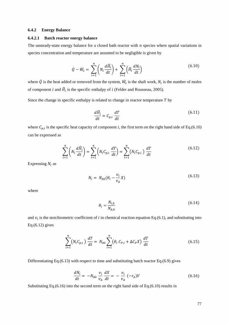
77

6.4.2 Energy Balance

6.4.2.1 Batch reactor energy balance

The unsteady-state energy balance for a closed bath reactor with 𝑛 species where spatial variations in

species concentration and temperature are assumed to be negligible is given by

where 𝑄ሶ is the heat added or removed from the system, 𝑊ሶ𝑠 is the shaft work, 𝑁𝑖 is the number of moles

of component 𝑖 and �̂�𝑖 is the specific enthalpy of 𝑖 (Felder and Rousseau, 2005).

Since the change in specific enthalpy is related to change in reactor temperature 𝑇 by

where 𝐶𝑝,𝑖 is the specific heat capacity of component 𝑖, the first term on the right hand side of Eq.(6.10)

can be expressed as

Expressing 𝑁𝑖 as

where

and 𝑣𝑖 is the stoichiometric coefficient of 𝑖 in chemical reaction equation Eq.(6.1), and substituting into

Eq.(6.12) gives

Differentiating Eq.(6.13) with respect to time and substituting batch reactor Eq.(6.9) gives

Substituting Eq.(6.16) into the second term on the right hand side of Eq.(6.10) results in

𝑄ሶ − 𝑊ሶ𝑠 = ∑ (𝑁𝑖

𝑑�̂�𝑖

𝑑𝑡)

𝑛

𝑖=1

+ ∑ (�̂�𝑖

𝑑𝑁𝑖

𝑑𝑡)

𝑛

𝑖=1

(6.10)

𝑑�̂�𝑖

𝑑𝑡= 𝐶𝑝,𝑖

𝑑𝑇

𝑑𝑡

(6.11)

∑ (𝑁𝑖

𝑑�̂�𝑖

𝑑𝑡)

𝑛

𝑖=1

= ∑ (𝑁𝑖𝐶𝑝,𝑖 𝑑𝑇

𝑑𝑡)

𝑛

𝑖=1

= ∑(𝑁𝑖𝐶𝑝,𝑖 )

𝑛

𝑖=1

𝑑𝑇

𝑑𝑡

(6.12)

𝑁𝑖 = 𝑁𝐴0(𝜃𝑖 −𝑣𝑖

𝑣𝐴𝑋) (6.13)

𝜃𝑖 =𝑁𝑖,0

𝑁𝐴,0

(6.14)

∑(𝑁𝑖𝐶𝑝,𝑖 )

𝑛

𝑖=1

𝑑𝑇

𝑑𝑡= 𝑁𝐴0 ∑(𝜃𝑖 𝐶𝑃,𝑖 + Δ𝐶𝑃𝑋)

𝑛

𝑖=1

𝑑𝑇

𝑑𝑡

(6.15)

𝑑𝑁𝑖

𝑑𝑡= −𝑁𝐴0

𝑣𝑖

𝑣𝐴 𝑑𝑋

𝑑𝑡= −

𝑣𝑖

𝑣𝐴 (−𝑟𝐴)𝑉 (6.16)

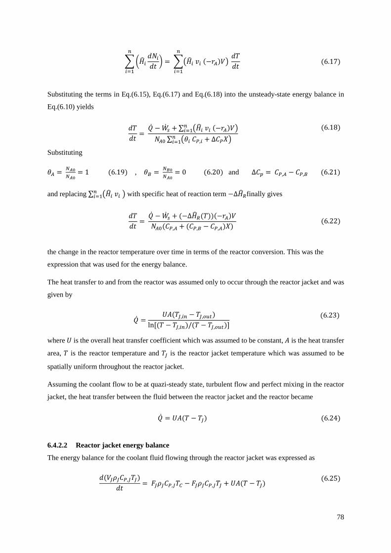
78

Substituting the terms in Eq.(6.15), Eq.(6.17) and Eq.(6.18) into the unsteady-state energy balance in

Eq.(6.10) yields

Substituting

𝜃𝐴 = 𝑁𝐴0

𝑁𝐴0= 1 (6.19) , 𝜃𝐵 =

𝑁𝐵0

𝑁𝐴0= 0 (6.20) and Δ𝐶𝑝 = 𝐶𝑃,𝐴 − 𝐶𝑃,𝐵 (6.21)

and replacing ∑ (�̂�𝑖 𝑣𝑖 )𝑛𝑖=1 with specific heat of reaction term −Δ�̂�𝑅finally gives

the change in the reactor temperature over time in terms of the reactor conversion. This was the

expression that was used for the energy balance.

The heat transfer to and from the reactor was assumed only to occur through the reactor jacket and was

given by

where 𝑈 is the overall heat transfer coefficient which was assumed to be constant, 𝐴 is the heat transfer

area, 𝑇 is the reactor temperature and 𝑇𝐽 is the reactor jacket temperature which was assumed to be

spatially uniform throughout the reactor jacket.

Assuming the coolant flow to be at quazi-steady state, turbulent flow and perfect mixing in the reactor

jacket, the heat transfer between the fluid between the reactor jacket and the reactor became

6.4.2.2 Reactor jacket energy balance

The energy balance for the coolant fluid flowing through the reactor jacket was expressed as

∑ (�̂�𝑖

𝑑𝑁𝑖

𝑑𝑡)

𝑛

𝑖=1

= ∑(�̂�𝑖 𝑣𝑖 (−𝑟𝐴)𝑉)

𝑛

𝑖=1

𝑑𝑇

𝑑𝑡

(6.17)

𝑑𝑇

𝑑𝑡=

𝑄ሶ − 𝑊ሶ𝑠 + ∑ (�̂�𝑖 𝑣𝑖 (−𝑟𝐴)𝑉)𝑛

𝑖=1

𝑁𝐴0 ∑ (𝜃𝑖 𝐶𝑃,𝑖 + Δ𝐶𝑃𝑋)𝑛𝑖=1

(6.18)

𝑑𝑇

𝑑𝑡=

𝑄ሶ − 𝑊ሶ𝑠 + (−Δ�̂�𝑅(𝑇))(−𝑟𝐴)𝑉

𝑁𝐴0(𝐶𝑃,𝐴 + (𝐶𝑃,𝐵 − 𝐶𝑃,𝐴)𝑋)

(6.22)

𝑄ሶ =𝑈𝐴(𝑇𝐽,𝑖𝑛 − 𝑇𝐽,𝑜𝑢𝑡)

ln [(𝑇 − 𝑇𝐽,𝑖𝑛)/(𝑇 − 𝑇𝐽,𝑜𝑢𝑡)]

(6.23)

𝑄ሶ = 𝑈𝐴(𝑇 − 𝑇𝐽)

(6.24)

𝑑(𝑉𝐽𝜌𝐽𝐶𝑃,𝐽𝑇𝐽)

𝑑𝑡= 𝐹𝐽𝜌𝐽𝐶𝑃,𝐽𝑇𝐶 − 𝐹𝐽𝜌𝐽𝐶𝑃,𝐽𝑇𝐽 + 𝑈𝐴(𝑇 − 𝑇𝐽)

(6.25)

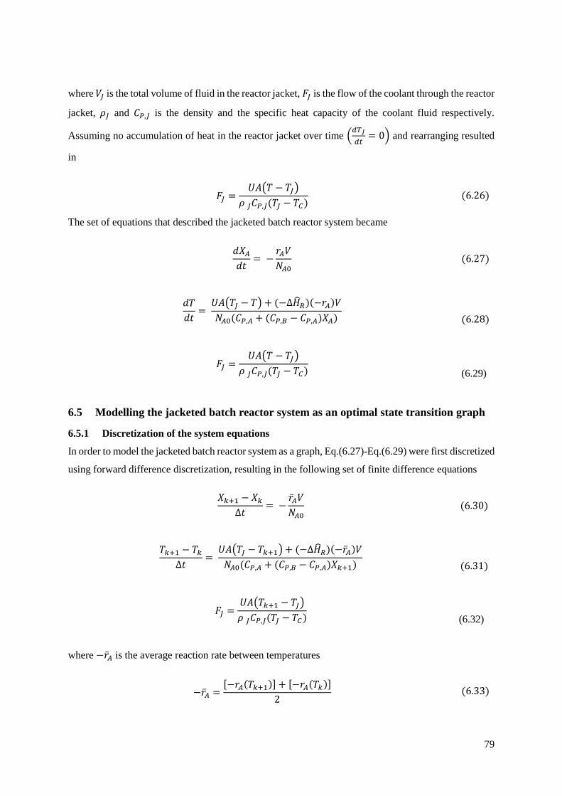
79

where 𝑉𝐽 is the total volume of fluid in the reactor jacket, 𝐹𝐽 is the flow of the coolant through the reactor

jacket, 𝜌𝐽 and 𝐶𝑃,𝐽 is the density and the specific heat capacity of the coolant fluid respectively.

Assuming no accumulation of heat in the reactor jacket over time (𝑑𝑇𝐽

𝑑𝑡= 0) and rearranging resulted

in

The set of equations that described the jacketed batch reactor system became

6.5 Modelling the jacketed batch reactor system as an optimal state transition graph

6.5.1 Discretization of the system equations

In order to model the jacketed batch reactor system as a graph, Eq.(6.27)-Eq.(6.29) were first discretized

using forward difference discretization, resulting in the following set of finite difference equations

where −�̅�𝐴 is the average reaction rate between temperatures

𝐹𝐽 =𝑈𝐴(𝑇 − 𝑇𝐽)

𝜌 𝐽𝐶𝑃,𝐽(𝑇𝐽 − 𝑇𝐶) (6.26)

𝑑𝑋𝐴

𝑑𝑡= −

𝑟𝐴𝑉

𝑁𝐴0

(6.27)

𝑑𝑇

𝑑𝑡=

𝑈𝐴(𝑇𝐽 − 𝑇) + (−Δ�̂�𝑅)(−𝑟𝐴)𝑉

𝑁𝐴0(𝐶𝑃,𝐴 + (𝐶𝑃,𝐵 − 𝐶𝑃,𝐴)𝑋𝐴)

(6.28)

𝐹𝐽 =𝑈𝐴(𝑇 − 𝑇𝐽)

𝜌 𝐽𝐶𝑃,𝐽(𝑇𝐽 − 𝑇𝐶)

(6.29)

𝑋𝑘+1 − 𝑋𝑘

Δ𝑡= −

�̅�𝐴𝑉

𝑁𝐴0

(6.30)

𝑇𝑘+1 − 𝑇𝑘

Δ𝑡=

𝑈𝐴(𝑇𝐽 − 𝑇𝑘+1) + (−Δ�̂�𝑅)(−�̅�𝐴)𝑉

𝑁𝐴0(𝐶𝑃,𝐴 + (𝐶𝑃,𝐵 − 𝐶𝑃,𝐴)𝑋𝑘+1)

(6.31)

𝐹𝐽 =𝑈𝐴(𝑇𝑘+1 − 𝑇𝐽)

𝜌 𝐽𝐶𝑃,𝐽(𝑇𝐽 − 𝑇𝐶)

(6.32)

−�̅�𝐴 =[−𝑟𝐴(𝑇𝑘+1)] + [−𝑟𝐴(𝑇𝑘)]

2

(6.33)

80

The discretized system state equations Eq.(6.30)-(6.33) in terms of the state transition 𝒙𝑖 → 𝒙𝑗 were

expressed as

where 𝑋𝑖 and 𝑇𝑖 are the conversion and temperature at vertex 𝑣𝑖, 𝑋𝑗 and 𝑇𝑗 is the conversion and

temperature at vertex 𝑣𝑗. 𝑇𝐽,𝑖𝑗 and 𝐹𝐽,𝑖𝑗 is the jacket side temperature and coolant flowrate that results in

the state transition.

6.5.2 Generating the graph of the dynamic system state space

The vertices, edges and edge weight function for OST Graph 𝐺 = (𝑉, 𝐸∗, 𝑊∗) of the jacketed batch

reactor system discrete dynamics were expressed as

The vertex set 𝑉 modelled a two dimensional discrete state space of points that were generated by

setting an upper and lower bound for the reactor temperature and the conversion of 𝐴, and selecting

values for the respective Δ𝑇 and Δ𝑋 step intervals. The vertices in 𝑉, optimal state transition edges 𝑒𝑖𝑗∗

and their respective optimal state transition weight function 𝑊𝑒𝑖𝑗∗ were generated through the procedure

in 4.4. In this system, the flow rate of the cooling fluid was taken as the only control variable thus

The constraints that were applied in generating the discrete state space and evaluating the optimal

weights for the OST Graph were

𝑋𝑗 − 𝑋𝑖

Δ𝑡= −

�̅�𝐴𝑉

𝑁𝐴0

(6.34)

𝑇𝑗 − 𝑇𝑖

Δ𝑡=

𝑈𝐴(𝑇𝐽,𝑖𝑗 − 𝑇𝑗) + (−Δ�̂�𝑅)(−�̅�𝐴)𝑉

𝑁𝐴0(𝐶𝑃,𝐴 + (𝐶𝑃,𝐵 − 𝐶𝑃,𝐴)𝑋𝑗)

(6.35)

𝐹𝐽,𝑖𝑗 = 𝒖𝑖𝑗 =𝑈𝐴(𝑇𝑗 − 𝑇𝐽,𝑖𝑗)

𝜌 𝐽𝐶𝑃,𝐽(𝑇𝐽,𝑖𝑗 − 𝑇𝐶) (6.36)

−�̅�𝐴 =[−𝑟𝐴(𝑇𝑗)] + [−𝑟𝐴(𝑇𝑖)]

2 (6.37)

𝑣𝑖 = [𝑇𝑖, 𝑋𝑖] 𝜖 𝑉 (6.38)

𝑒𝑖𝑗∗ = (𝑣𝑖 , 𝑣𝑗, 𝑤𝑖𝑗

∗ , 𝒖𝑖𝑗∗ , Δ𝑡𝑖𝑗

∗ ) 𝜖 𝐸∗

(6.39)

𝑊𝑒𝑖𝑗∗ = ⟨𝑢𝑖𝑗

∗ , Δt𝑖𝑗∗ , 𝑐𝑖𝑗

∗ ⟩ (6.40)

𝒖𝑖𝑗∗ = 𝑢𝑖𝑗

∗ = 𝐹𝐽,𝑖𝑗∗ (6.41)

0 ≤ 𝑋 ≤ 1.0 (6.42)

300 ≤ 𝑇 ≤ 360 𝐾 (6.43)

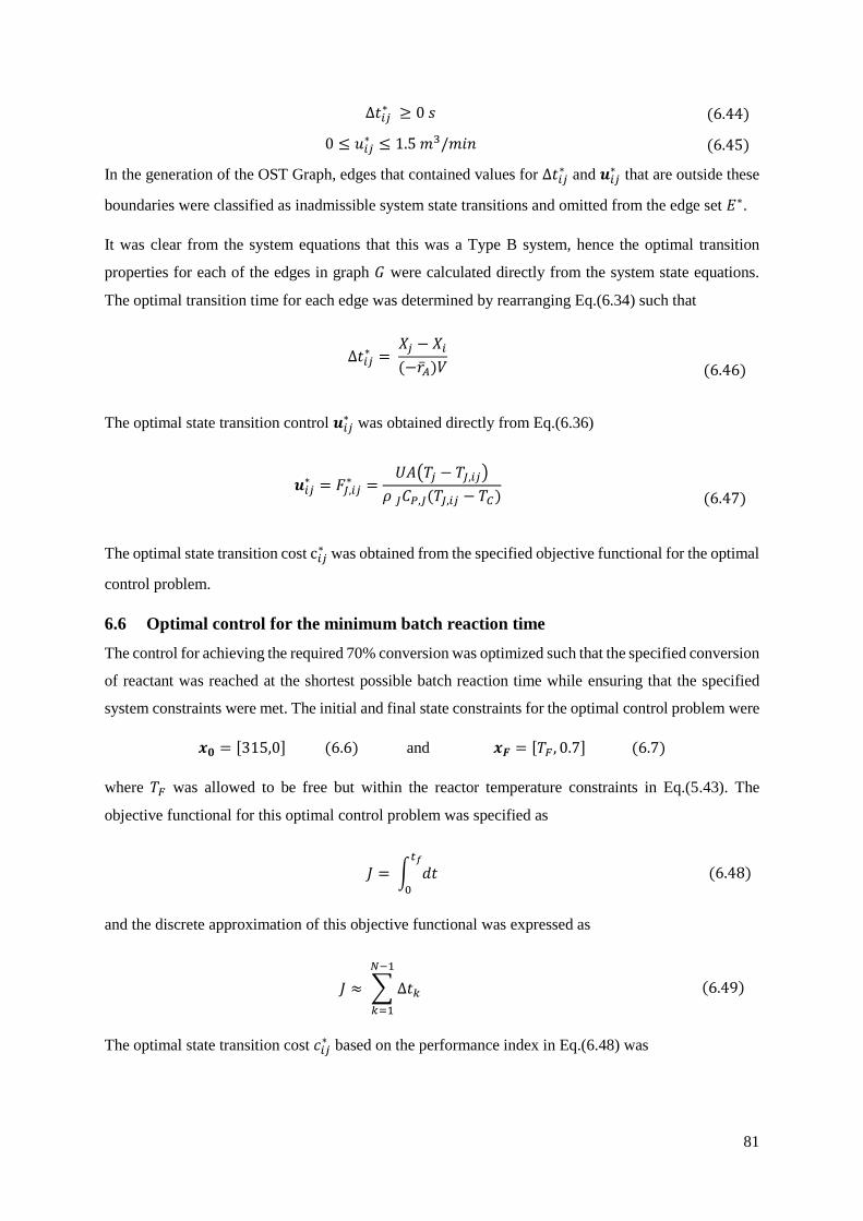
81

In the generation of the OST Graph, edges that contained values for Δ𝑡𝑖𝑗∗ and 𝒖𝑖𝑗

∗ that are outside these

boundaries were classified as inadmissible system state transitions and omitted from the edge set 𝐸∗.

It was clear from the system equations that this was a Type B system, hence the optimal transition

properties for each of the edges in graph 𝐺 were calculated directly from the system state equations.

The optimal transition time for each edge was determined by rearranging Eq.(6.34) such that

The optimal state transition control 𝒖𝑖𝑗∗ was obtained directly from Eq.(6.36)

The optimal state transition cost c𝑖𝑗∗ was obtained from the specified objective functional for the optimal

control problem.

6.6 Optimal control for the minimum batch reaction time

The control for achieving the required 70% conversion was optimized such that the specified conversion

of reactant was reached at the shortest possible batch reaction time while ensuring that the specified

system constraints were met. The initial and final state constraints for the optimal control problem were

𝒙𝟎 = [315,0] (6.6) and 𝒙𝑭 = [𝑇𝐹 , 0.7] (6.7)

where 𝑇𝐹 was allowed to be free but within the reactor temperature constraints in Eq.(5.43). The

objective functional for this optimal control problem was specified as

and the discrete approximation of this objective functional was expressed as

The optimal state transition cost 𝑐𝑖𝑗∗ based on the performance index in Eq.(6.48) was

Δ𝑡𝑖𝑗∗ ≥ 0 𝑠 (6.44)

0 ≤ 𝑢𝑖𝑗∗ ≤ 1.5 𝑚3/𝑚𝑖𝑛 (6.45)

Δ𝑡𝑖𝑗∗ =

𝑋𝑗 − 𝑋𝑖

(−�̅�𝐴)𝑉

(6.46)

𝒖𝑖𝑗∗ = 𝐹𝐽,𝑖𝑗

∗ =𝑈𝐴(𝑇𝑗 − 𝑇𝐽,𝑖𝑗)

𝜌 𝐽𝐶𝑃,𝐽(𝑇𝐽,𝑖𝑗 − 𝑇𝐶)

(6.47)

𝐽 = ∫ 𝑑𝑡𝑡𝑓

0

(6.48)

𝐽 ≈ ∑ Δ𝑡𝑘

𝑁−1

𝑘=1

(6.49)

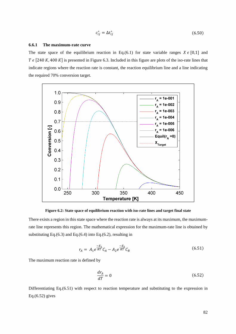
82

6.6.1 The maximum-rate curve

The state space of the equilibrium reaction in Eq.(6.1) for state variable ranges 𝑋 𝜖 [0,1] and

𝑇 𝜖 [240 𝐾, 400 𝐾] is presented in Figure 6.3. Included in this figure are plots of the iso-rate lines that

indicate regions where the reaction rate is constant, the reaction equilibrium line and a line indicating

the required 70% conversion target.

Figure 6.2: State space of equilibrium reaction with iso-rate lines and target final state

There exists a region in this state space where the reaction rate is always at its maximum, the maximum-

rate line represents this region. The mathematical expression for the maximum-rate line is obtained by

substituting Eq.(6.3) and Eq.(6.4) into Eq.(6.2), resulting in

The maximum reaction rate is defined by

Differentiating Eq.(6.51) with respect to reaction temperature and substituting to the expression in

Eq.(6.52) gives

𝑐𝑖𝑗∗ = Δ𝑡𝑖𝑗

∗ (6.50)

𝑟𝐴 = 𝐴1𝑒−𝐸1𝑅𝑇 𝐶𝐴 − 𝐴2𝑒

−𝐸2𝑅𝑇 𝐶𝐵 (6.51)

𝑑𝑟𝐴

𝑑𝑇= 0 (6.52)

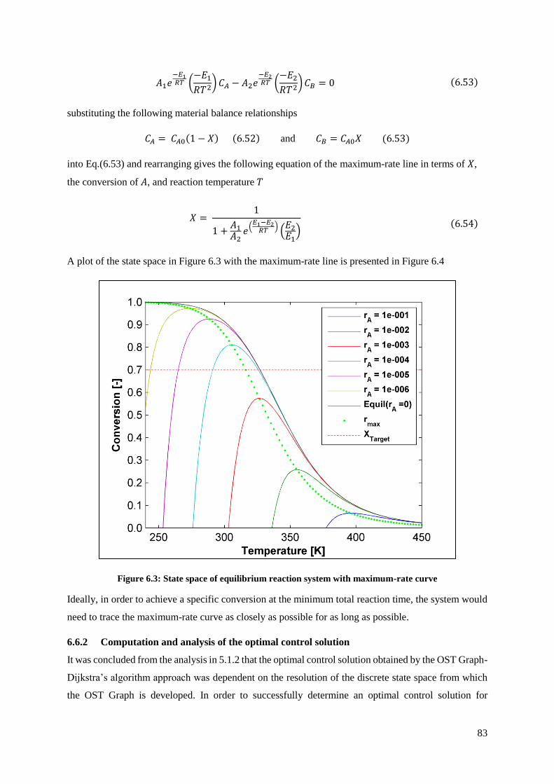
83

substituting the following material balance relationships

𝐶𝐴 = 𝐶𝐴0(1 − 𝑋) (6.52) and 𝐶𝐵 = 𝐶𝐴0𝑋 (6.53)

into Eq.(6.53) and rearranging gives the following equation of the maximum-rate line in terms of 𝑋,

the conversion of 𝐴, and reaction temperature 𝑇

A plot of the state space in Figure 6.3 with the maximum-rate line is presented in Figure 6.4

Figure 6.3: State space of equilibrium reaction system with maximum-rate curve

Ideally, in order to achieve a specific conversion at the minimum total reaction time, the system would

need to trace the maximum-rate curve as closely as possible for as long as possible.

6.6.2 Computation and analysis of the optimal control solution

It was concluded from the analysis in 5.1.2 that the optimal control solution obtained by the OST Graph-

Dijkstra’s algorithm approach was dependent on the resolution of the discrete state space from which

the OST Graph is developed. In order to successfully determine an optimal control solution for

𝐴1𝑒−𝐸1𝑅𝑇 (

−𝐸1

𝑅𝑇2) 𝐶𝐴 − 𝐴2𝑒

−𝐸2𝑅𝑇 (

−𝐸2

𝑅𝑇2) 𝐶𝐵 = 0 (6.53)

𝑋 = 1

1 +𝐴1𝐴2

𝑒(

𝐸1−𝐸2𝑅𝑇

)(

𝐸2𝐸1

)

(6.54)

84

achieving a conversion 𝑋 = 0.7 at the minimum batch reaction time, the resolution for the discrete state

space from which the OST Graph was developed needed be selected such that

• State space trajectories from the initial state 𝒙𝟎 = [300,0] to final states 𝒙𝑭 = [𝑇𝐹, 0.7],

where 𝑇𝐹 is a free variable, existed.

• The discrete state space resulted in an OST Graph with a reasonable number of edges

and vertices to allow for an optimal control solution to be determined by Dijkstra’s

algorithm in a computation time that was reasonable for realistic implementation

• The resultant optimal control solution satisfied the batch reactor system constraints and

could be practically implemented to the batch reactor system through open loop control

An investigation was conducted to determine a discrete state space resolution that effectively satisfied

the above listed criteria. This was done by

• Selecting state variable interval pairs [Δ𝑇, Δ𝑋] for discrete state space grid resolutions

• Generating OST Graphs for the respective resolutions to model the optimal state transition

dynamics between the points in the respective discrete state spaces and,

• Applying Dijkstra’s Algorithm to determine the shortest path from the initial vertex

𝑣0⟨𝒙𝟎 = [315,0]⟩ to every other reachable vertex 𝑣𝐹⟨𝒙𝑭 = [𝑇𝐹 , 0.7]⟩ for each of the generated

OST Graphs. This gave multiple shortest path solutions for each OST Graph as there existed

multiple states for which 𝑋= 0.7, at various final reactor temperatures.

• Selecting the optimal final vertex 𝑣𝐹∗⟨𝒙𝑭

∗ = [𝑇𝐹∗, 0.7]⟩ that gave the shortest path cost 𝐶∗(𝑣𝐹

∗)

from 𝑣0 for each OST Graph

• The optimal control solutions from the shortest paths that resulted in the costs 𝐶∗(𝑣𝐹∗) for each

of the OST Graphs were then analysed to determine whether an optimal control solution existed

and compared to determine the OST Graph resolution that provided the best result

The simulations for generating the discrete state space, modelling the dynamics as an the OST Graph

and determining the optimal path by applying Dijkstra’s Algorithm were conducted in the simulation

conditions specified in section 5.1. The upper and lower limits of 𝑇𝜖[240 𝐾, 400 𝐾] and 𝑋𝜖[0 − 1]

were used for generating the discrete state spaces. The table of results for the investigation of the

solution feasibility for the different state space resolutions is presented in Table 6.2.

The results in Table 6.2 show that OST Graphs that were generated for the various discrete state space

resolutions had significantly low average node degrees. The low average node degrees were a result of

the nature of the dynamic system. Due to the forward reaction being exothermic and the reverse reaction

being endothermic, a change in the temperature of the reactor system always resulted in a change in the

conversion and a change in the conversion always resulted in a change in the reactor temperature.

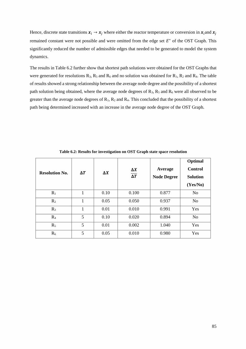
85

Hence, discrete state transitions 𝒙𝑖 → 𝒙𝑗 where either the reactor temperature or conversion in 𝒙𝑖and 𝒙𝑗

remained constant were not possible and were omitted from the edge set 𝐸∗ of the OST Graph. This

significantly reduced the number of admissible edges that needed to be generated to model the system

dynamics.

The results in Table 6.2 further show that shortest path solutions were obtained for the OST Graphs that

were generated for resolutions R3, R5 and R6 and no solution was obtained for R1, R2 and R4. The table

of results showed a strong relationship between the average node degree and the possibility of a shortest

path solution being obtained, where the average node degrees of R3, R5 and R6 were all observed to be

greater than the average node degrees of R1, R2 and R4. This concluded that the possibility of a shortest

path being determined increased with an increase in the average node degree of the OST Graph.

Table 6.2: Results for investigation on OST Graph state space resolution

Resolution No. 𝚫𝑻 𝚫𝑿 𝚫𝑿

𝚫𝑻

Average

Node Degree

Optimal

Control

Solution

(Yes/No)

R1 1 0.10 0.100 0.877 No

R2 1 0.05 0.050 0.937 No

R3 1 0.01 0.010 0.991 Yes

R4 5 0.10 0.020 0.894 No

R5 5 0.01 0.002 1.040 Yes

R6 5 0.05 0.010 0.980 Yes

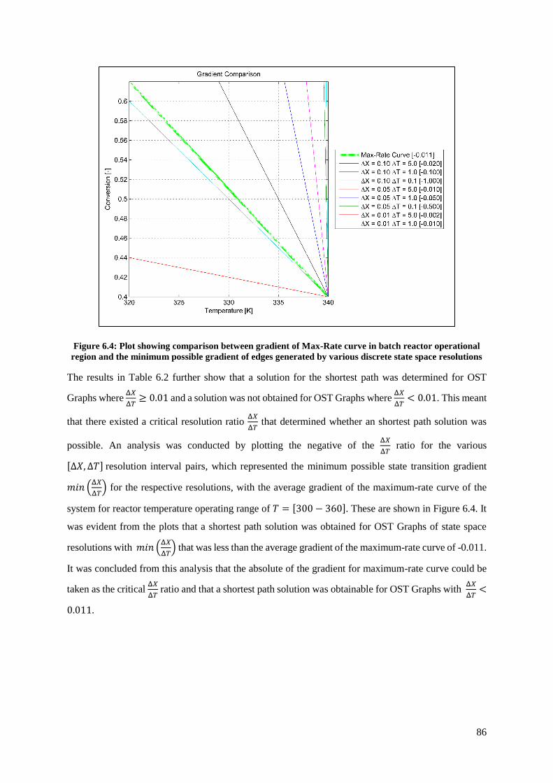
86

Figure 6.4: Plot showing comparison between gradient of Max-Rate curve in batch reactor operational

region and the minimum possible gradient of edges generated by various discrete state space resolutions

The results in Table 6.2 further show that a solution for the shortest path was determined for OST

Graphs where Δ𝑋

Δ𝑇≥ 0.01 and a solution was not obtained for OST Graphs where

Δ𝑋

Δ𝑇< 0.01. This meant

that there existed a critical resolution ratio Δ𝑋

Δ𝑇 that determined whether an shortest path solution was

possible. An analysis was conducted by plotting the negative of the Δ𝑋

Δ𝑇 ratio for the various

[Δ𝑋, Δ𝑇] resolution interval pairs, which represented the minimum possible state transition gradient

𝑚𝑖𝑛 (Δ𝑋

Δ𝑇) for the respective resolutions, with the average gradient of the maximum-rate curve of the

system for reactor temperature operating range of 𝑇 = [300 − 360]. These are shown in Figure 6.4. It

was evident from the plots that a shortest path solution was obtained for OST Graphs of state space

resolutions with 𝑚𝑖𝑛 (Δ𝑋

Δ𝑇) that was less than the average gradient of the maximum-rate curve of -0.011.

It was concluded from this analysis that the absolute of the gradient for maximum-rate curve could be

taken as the critical Δ𝑋

Δ𝑇 ratio and that a shortest path solution was obtainable for OST Graphs with

Δ𝑋

Δ𝑇<

0.011.

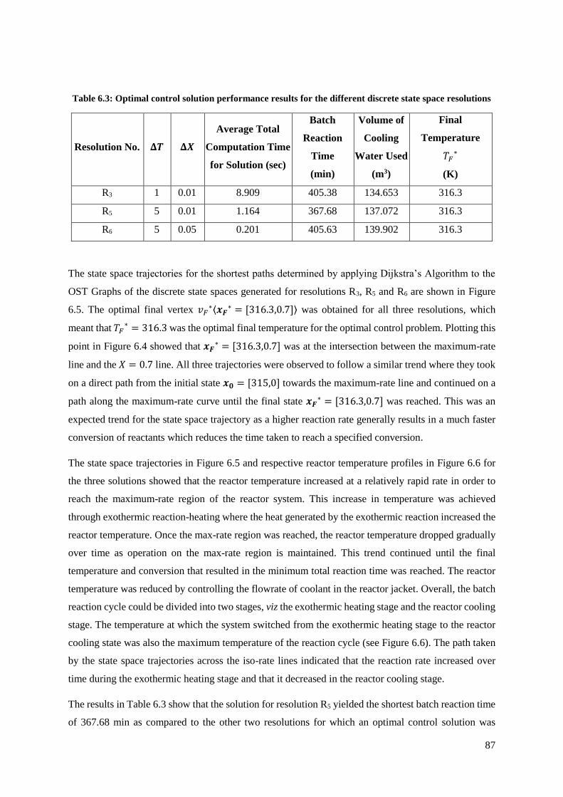
87

Table 6.3: Optimal control solution performance results for the different discrete state space resolutions

Resolution No. 𝚫𝑻 𝚫𝑿

Average Total

Computation Time

for Solution (sec)

Batch

Reaction

Time

(min)

Volume of

Cooling

Water Used

(m3)

Final

Temperature

𝑇𝐹∗

(K)

R3 1 0.01 8.909 405.38 134.653 316.3

R5 5 0.01 1.164 367.68 137.072 316.3

R6 5 0.05 0.201 405.63 139.902 316.3

The state space trajectories for the shortest paths determined by applying Dijkstra’s Algorithm to the

OST Graphs of the discrete state spaces generated for resolutions R3, R5 and R6 are shown in Figure

6.5. The optimal final vertex 𝑣𝐹∗⟨𝒙𝑭

∗ = [316.3,0.7]⟩ was obtained for all three resolutions, which

meant that 𝑇𝐹∗ = 316.3 was the optimal final temperature for the optimal control problem. Plotting this

point in Figure 6.4 showed that 𝒙𝑭∗ = [316.3,0.7] was at the intersection between the maximum-rate

line and the 𝑋 = 0.7 line. All three trajectories were observed to follow a similar trend where they took

on a direct path from the initial state 𝒙𝟎 = [315,0] towards the maximum-rate line and continued on a

path along the maximum-rate curve until the final state 𝒙𝑭∗ = [316.3,0.7] was reached. This was an

expected trend for the state space trajectory as a higher reaction rate generally results in a much faster

conversion of reactants which reduces the time taken to reach a specified conversion.

The state space trajectories in Figure 6.5 and respective reactor temperature profiles in Figure 6.6 for

the three solutions showed that the reactor temperature increased at a relatively rapid rate in order to

reach the maximum-rate region of the reactor system. This increase in temperature was achieved

through exothermic reaction-heating where the heat generated by the exothermic reaction increased the

reactor temperature. Once the max-rate region was reached, the reactor temperature dropped gradually

over time as operation on the max-rate region is maintained. This trend continued until the final

temperature and conversion that resulted in the minimum total reaction time was reached. The reactor

temperature was reduced by controlling the flowrate of coolant in the reactor jacket. Overall, the batch

reaction cycle could be divided into two stages, viz the exothermic heating stage and the reactor cooling

stage. The temperature at which the system switched from the exothermic heating stage to the reactor

cooling state was also the maximum temperature of the reaction cycle (see Figure 6.6). The path taken

by the state space trajectories across the iso-rate lines indicated that the reaction rate increased over

time during the exothermic heating stage and that it decreased in the reactor cooling stage.

The results in Table 6.3 show that the solution for resolution R5 yielded the shortest batch reaction time

of 367.68 min as compared to the other two resolutions for which an optimal control solution was

88

determined. This was a result of the trajectory solution for R5 taking a much shorter time to reach the

max-rate region and a greater proportion of the total reaction cycle time being spent in the reactor

cooling stage of the batch reaction cycle when compared to R3 and R6. This was further observed in

Figure 6.5 and Figure 6.6. The solutions obtained for resolutions R3 and R6 both had a similar proportion

of the total reaction cycle time being spent in the exothermic heating and reactor cooling stage but the

former resulted in a slightly improved reaction cycle time. This was due the R3 being much finer

resolution which allowed the solution of its state space trajectory to follow the maximum-rate line more

effectively (see Figure 6.5).

The plots of control over time in Figure 6.7 for the optimal control solutions obtained for R3, R5 and R6

resulted in similar trends for the reactor coolant flowrate. Initially, the coolant flowrate increased rapidly

over time when the reactor operated in the exothermic heating stage to a maximum flowrate that was

reached at the maximum reaction temperature. The flowrate was then dropped gradually over time for

the reactor cooling stage until the final system state is reached. The rapid increase in the coolant flowrate

for the exothermic heating stage regulated the increase in the rate at which heat was generated by the

increase in the reaction rate as the system approached the maximum rate region. The gradual

temperature drop experienced in the reactor cooling stage was due to the decrease in the rate of reaction

and heat generation that took place over time as the concentration of 𝐴 decreased.

When selecting the discrete state space resolution for the specified batch reaction time optimization

optimal control problem, the preferred resolution was that which had a solution with the lowest reaction

cycle time. However the physical limitations of the system also needed to be accounted for, which, in

the context of the designed jacketed batch reactor system, was the specified reaction temperature limit

of 360K and the allowed maximum coolant flowrate of 1.5 m3/min.

It is clear that the resolution R5 provided an optimal solution with respect to batch reaction time.

However the optimal state space trajectories presented in Figure 6.4 and the reactor temperature profile

in Figure 6.5 show that the state space trajectory obtained for this resolution resulted in a reactor

temperature that exceeded the 360K critical reaction temperature limit. Applying this solution to the

designed batch reactor system would trigger the split-range temperature controller to reduce the reactor

temperature back to safe operating conditions, thus disrupting the intended optimal trajectory of the

system state through the state space and resulting in non-optimal operation. Solutions obtained for

resolutions R3 and R6 resulted in a much greater reaction cycle time when compared to R5 but satisfied

the reaction temperature limit requirement. The solution for resolution R3 had a greater batch reaction

time and used less cooling water when compared to R5 as shown in Table 6.3. The batch reaction time

obtained for R3 was 9.3% greater and the total water usage was 1.76% less than that which was obtained

for R5. R5 provided a much better computational performance when compared to R3 due to the fewer

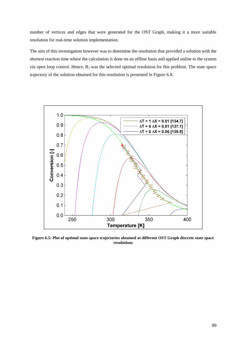
89

number of vertices and edges that were generated for the OST Graph, making it a more suitable

resolution for real-time solution implementation.

The aim of this investigation however was to determine the resolution that provided a solution with the

shortest reaction time where the calculation is done on an offline basis and applied online to the system

via open loop control. Hence, R3 was the selected optimal resolution for this problem. The state space

trajectory of the solution obtained for this resolution is presented in Figure 6.8.

Figure 6.5: Plot of optimal state space trajectories obtained at different OST Graph discrete state space

resolutions

90

Figure 6.6: Optimal reactor temperature profiles for the different discrete state space resolutions

Figure 6.7: Optimal coolant flowrate as a function of time for the different discrete state space resolutions

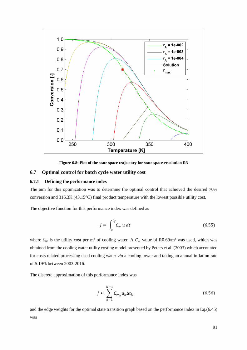
91

Figure 6.8: Plot of the state space trajectory for state space resolution R3

6.7 Optimal control for batch cycle water utility cost

6.7.1 Defining the performance index

The aim for this optimization was to determine the optimal control that achieved the desired 70%

conversion and 316.3K (43.15°C) final product temperature with the lowest possible utility cost.

The objective function for this performance index was defined as

where 𝐶𝑤 is the utility cost per m3 of cooling water. A 𝐶𝑤 value of R0.69/m3 was used, which was

obtained from the cooling water utility costing model presented by Peters et al. (2003) which accounted

for costs related processing used cooling water via a cooling tower and taking an annual inflation rate

of 5.19% between 2003-2016.

The discrete approximation of this performance index was

and the edge weights for the optimal state transition graph based on the performance index in Eq.(6.45)

was

𝐽 = ∫ 𝐶𝑤 𝑢 𝑑𝑡𝑡𝑓

0

(6.55)

𝐽 ≈ ∑ 𝐶𝑤𝑘𝑢𝑘Δ𝑡𝑘

𝑁−1

𝑘=1

(6.56)

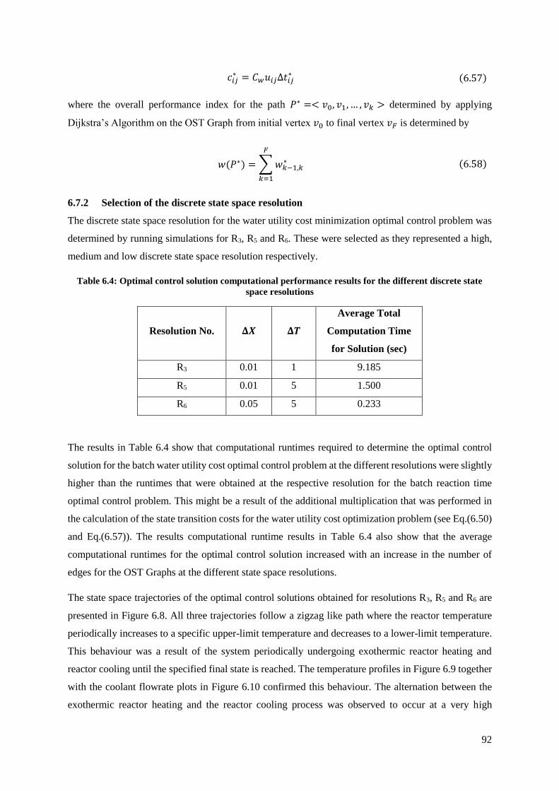
92

where the overall performance index for the path 𝑃∗ =< 𝑣0, 𝑣1, … , 𝑣𝑘 > determined by applying

Dijkstra’s Algorithm on the OST Graph from initial vertex 𝑣0 to final vertex 𝑣𝐹 is determined by

6.7.2 Selection of the discrete state space resolution

The discrete state space resolution for the water utility cost minimization optimal control problem was

determined by running simulations for R3, R5 and R6. These were selected as they represented a high,

medium and low discrete state space resolution respectively.

Table 6.4: Optimal control solution computational performance results for the different discrete state

space resolutions

Resolution No. 𝚫𝑿 𝚫𝑻

Average Total

Computation Time

for Solution (sec)

R3 0.01 1 9.185

R5 0.01 5 1.500

R6 0.05 5 0.233

The results in Table 6.4 show that computational runtimes required to determine the optimal control

solution for the batch water utility cost optimal control problem at the different resolutions were slightly

higher than the runtimes that were obtained at the respective resolution for the batch reaction time

optimal control problem. This might be a result of the additional multiplication that was performed in

the calculation of the state transition costs for the water utility cost optimization problem (see Eq.(6.50)

and Eq.(6.57)). The results computational runtime results in Table 6.4 also show that the average

computational runtimes for the optimal control solution increased with an increase in the number of

edges for the OST Graphs at the different state space resolutions.

The state space trajectories of the optimal control solutions obtained for resolutions R3, R5 and R6 are

presented in Figure 6.8. All three trajectories follow a zigzag like path where the reactor temperature

periodically increases to a specific upper-limit temperature and decreases to a lower-limit temperature.

This behaviour was a result of the system periodically undergoing exothermic reactor heating and

reactor cooling until the specified final state is reached. The temperature profiles in Figure 6.9 together

with the coolant flowrate plots in Figure 6.10 confirmed this behaviour. The alternation between the

exothermic reactor heating and the reactor cooling process was observed to occur at a very high

𝑐𝑖𝑗∗ = 𝐶𝑤𝑢𝑖𝑗Δ𝑡𝑖𝑗

∗ (6.57)

𝑤(𝑃∗) = ∑ 𝑤𝑘−1,𝑘∗

𝐹

𝑘=1

(6.58)

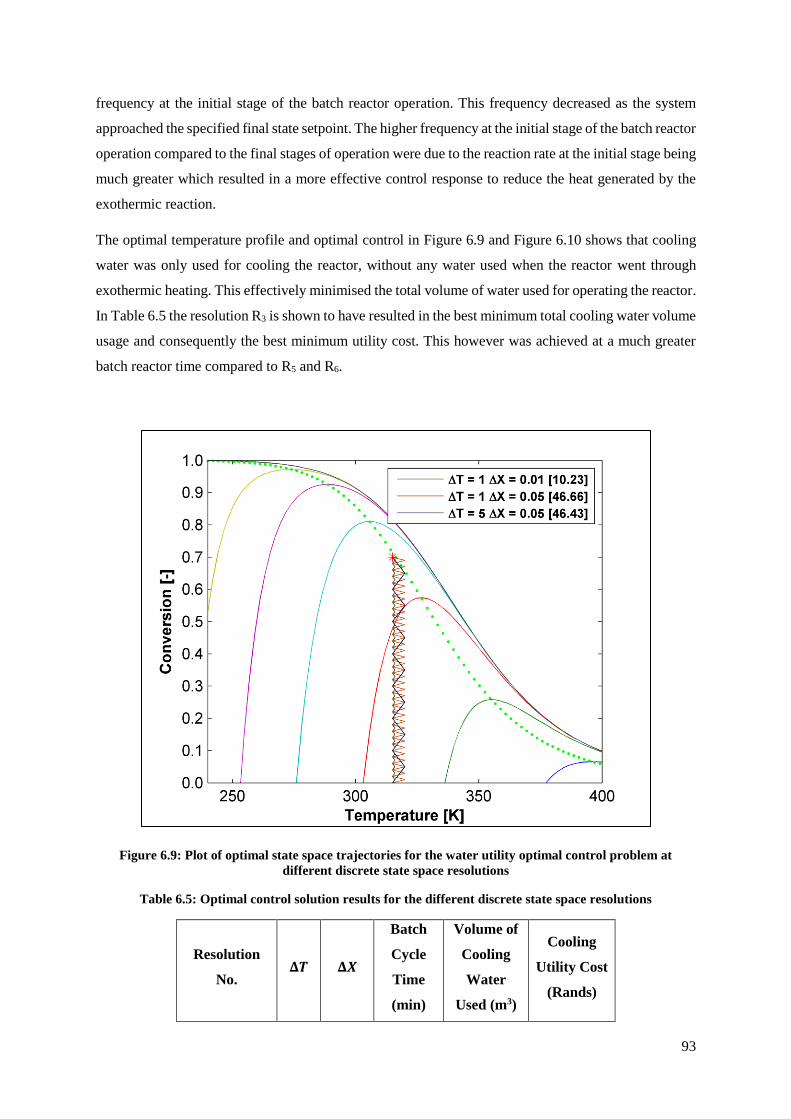
93

frequency at the initial stage of the batch reactor operation. This frequency decreased as the system

approached the specified final state setpoint. The higher frequency at the initial stage of the batch reactor

operation compared to the final stages of operation were due to the reaction rate at the initial stage being

much greater which resulted in a more effective control response to reduce the heat generated by the

exothermic reaction.

The optimal temperature profile and optimal control in Figure 6.9 and Figure 6.10 shows that cooling

water was only used for cooling the reactor, without any water used when the reactor went through

exothermic heating. This effectively minimised the total volume of water used for operating the reactor.

In Table 6.5 the resolution R3 is shown to have resulted in the best minimum total cooling water volume

usage and consequently the best minimum utility cost. This however was achieved at a much greater

batch reactor time compared to R5 and R6.

Figure 6.9: Plot of optimal state space trajectories for the water utility optimal control problem at

different discrete state space resolutions

Table 6.5: Optimal control solution results for the different discrete state space resolutions

Resolution

No. 𝚫𝑻 𝚫𝑿

Batch

Cycle

Time

(min)

Volume of

Cooling

Water

Used (m3)

Cooling

Utility Cost

(Rands)

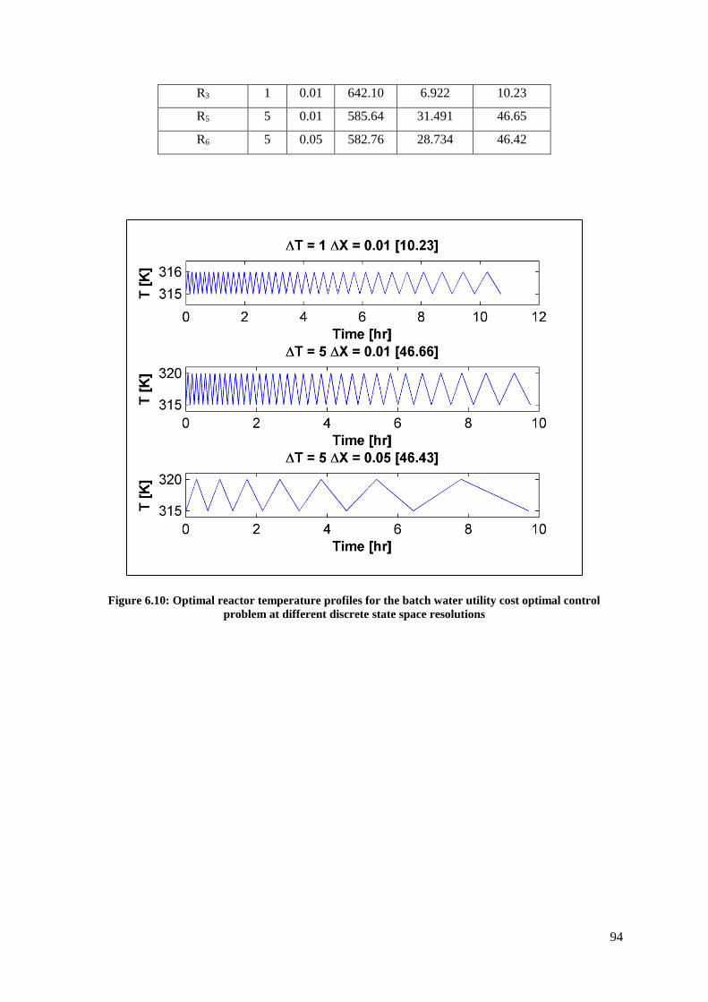
94

R3 1 0.01 642.10 6.922 10.23

R5 5 0.01 585.64 31.491 46.65

R6 5 0.05 582.76 28.734 46.42

Figure 6.10: Optimal reactor temperature profiles for the batch water utility cost optimal control

problem at different discrete state space resolutions

95

Figure 6.11: Optimal coolant flowrate as a function of time for the batch water utility cost optimal control

problem at different discrete state space resolutions

96

7 CONCLUSIONS

In this work, it was shown that it is possible to model a chemical process-based dynamic system as

weighted directed graph and that applying Dijkstra’s algorithm to the graph can

solve optimal control problems based on the dynamic system. An approach was successfully developed

for modelling the dynamic system as a weighted directed graph by defining an operating region for the

system dynamics, representing it as a discrete state space of points, and representing these state points

as graph vertices and the transition between the state points as weighted edges. The weighted edges

successfully represented the transition time, control input and state transition cost (based on the

objective functional of the defined problem) associated with each transition through the specification

of an edge weight function.

The optimal control problem was successfully reformulated into a shortest path graph search problem

by incorporating the objective functional to be represented by the state transition cost edge weight and

optimizing the edge weights. A method was developed for optimizing the state transitions across the

state space such that the transition time and control inputs stored in each edge weight were of the optimal

possible state transition for the defined objective functional, resulting in the Optimal State Transition

Graph (OST Graph). Applying Dijkstra’s algorithm to an OST Graph determined shortest paths from

an initial vertex to every other vertex in the graph. These shortest paths represented the optimal

trajectories from an initial state to every other state in the dynamic system state space. The optimal

control for these optimal trajectories was determined by extracting the discrete controls from the

sequence of edges that resulted in the respective optimal paths. It hence was concluded that an optimal

control problem could be solved as a shortest path graph search problem.

The results from the tests that were made for comparing the OST Graph-Dijkstra’s Algorithm approach

with the calculus of variations, iterative dynamic programming and value iteration based dynamic

programming approach showed that the developed method successfully determined solutions to optimal

control problems for systems described by non-linear DAE’s. This included problems that were non-

linear and with constraints. The OST Graph-Dijkstra’s Algorithm approach proved to be finite in nature

thus guaranteeing convergence with a globally optimal solution being successfully determined as a

result of the global nature of Dijkstra’s algorithm. It is noted, however, that the solution was globally

optimal subject to the discretization applied when developing the optimal transition graph.

The results for simulation and control optimization of a linear nuclear reactor system showed that the

OST Graph- Dijkstra’s algorithm approach obtained a solution that was 0.39% more optimal than the

Iterative Dynamic Programming approach. The results from the simulation and control optimization of

a more complex non-linear jacketed continuous stirred reactor system showed that optimal control

solution obtained by OST Graph-Dijkstra’s algorithm approach provided a 14.74% improvement in the

minimization of the objective functional compared to the calculus of variations approach. In a

97

simulation that was further done on this system, the OST Graph-Dijkstra’s Algorithm approach obtained

the same minimum objective functional as the globally optimal solution based value-iteration Dynamic

Programming approach which confirmed that the developed approach determined a globally optimal

control solution. It is noted, however, that the solution was globally optimal subject to the discretization

that was applied in these approaches. The OST Graph determined an optimal control solution in a

computational runtime of 2 min 25.81s compared to the runtime of 29 hr 20 min 47.32s that was

required by the value-iteration based dynamic programming approach.

The analysis of simulations of the OST Graph-Dijkstra’s Algorithm approach showed that the

optimality of the minimum objective functional for an obtained solution is dependent on the state

variable increments used in defining the discrete state space resolution from which the OST Graph was

generated. It therefore could be concluded that the discrete state space resolution for the OST Graph

would need also to be optimized in order to obtain better optimality in the optimal control solutions.

The computations in this work were successfully performed on a personal computer and the solutions

were obtained at computational runtimes that were suitable for implementation, where an optimal

control solution could be determined from the model of the dynamic system and then applied as an

open-loop control. The number of vertices and edges, however, are expected to increase exponentially

with the number of state variables. This will result in much larger OST Graphs being generated as the

dimensions of the system state space increases, subsequently resulting in the computational runtime and

computational memory being required to determine an optimal path through the graph being

impractical. It should be noted that this issue is not particular to the approach presented here, but is a

general problem in optimal control theory.

98

8 RECOMMENDATIONS

It should be noted that there still remains much room for improvement in the developed approach to

solving optimal control problems. At the current stage of development, the computational runtime time

required to obtain an optimal control solution for the studied systems makes it more suitable for the

optimal control policy to be determined in an offline based simulation and then being applied to the

physical system after the control policy has been fully determined.

The saturation in the computer’s volatile memory (RAM) when generating the OST Graph can be

resolved by retaining only the previous and present states of the system for each respective computation

of the optimal state transition edge weights (for time, control and cost), and storing the values obtained

into physical (swap) memory. This approach is expected to significantly increase the number of states

and state transitions for which the OST Graph model can be generated, however, this would

significantly increase the computation time required to compute the optimal state transition graph due

to physical memory being much slower for the computational processor to access than volatile memory.

This approach can also be applied in the calculation of the shortest path by Dijkstra’s algorithm but may

result in computational runtimes that are impractical for implementation if the number of vertices and

edges for the OST Graph are too large.

Computational acceleration methods such as parallel processing and utilizing more efficient data

structures to represent the graph vertices and edges provide much room for improvement in terms of

required system memory and number of computations required for determining optimal control policies.

Parallel processing can be applied in the generation of the OST Graph by partitioning the total number

of graph vertices over 𝑛 processors and computing their respective optimal state transition edge weights

(for time, control and cost) independently. This is possible because the edge weights are only dependent

on the initial and final state of the respective transitions that they represent. Utilizing these techniques

provide great potential for making the real-time implementation of the developed method feasible.

Dijkstra’s algorithm is a highly sequential algorithm which makes it difficult to parallelize. Attempts to

parallelize the algorithm have proven to provide minimal improvement in computational runtime

(Jasika et al., 2012; Crauser et al., 1998). The alternatives for improving performance for the shortest

path search include Bidirectional Dijkstra’s Algorithm and the heuristic based A* algorithm which have

proven to result in considerable reduction in the computation time (Russell & Norvig, 2002).

99

9 REFERENCES

Aggarwal, A., Anderson, R.J. & Kao, M.-Y. 1989. Parallel depth-first search in general directed graphs.

In Proceedings of the twenty-first annual ACM symposium on Theory of computing. 297–308.

Ahuja, R.K., Mehlhorn, K., Orlin, J. & Tarjan, R.E. 1990. Faster algorithms for the shortest path

problem. Journal of the ACM (JACM), 37(2): 213–223.

Appel, K.I. & Haken, W. 1989. Every planar map is four colorable. American Mathematical Society

Providence.

Aris, R. & Amundson, N.R. 1958. An analysis of chemical reactor stability and control—I: The

possibility of local control, with perfect or imperfect control mechanisms. Chemical Engineering

Science, 7(3): 121–131.

Ascher, U.M. & Petzold, L.R. 1998. Computer Methods for Ordinary Differential Equations and

Differential-Algebraic Equations. Siam.

Bales, M.E. & Johnson, S.B. 2006. Graph theoretic modeling of large-scale semantic networks. Journal

of Biomedical Informatics, 39(4): 451–464.

Ball, W.W.R. 1892. Mathematical recreations and problems of past and present times. Macmillan and

Company.

Bannister, M.J. & Eppstein, D. 2012. Randomized speedup of the bellman-ford algorithm. In

Proceedings of the Meeting on Analytic Algorithmics and Combinatorics. 41–47.

Barbehenn, M. 1998. A note on the complexity of Dijkstra’s algorithm for graphs with weighted

vertices. IEEE Transactions on Computers, 47(2): 263.

Bellman, R. 1958. On a routing problem. Quarterly of applied mathematics: 87–90.

Bellman, R. 1954. The Theory of Dynamic Programming. Bulletin of the American Mathematical

Society, 60(6): 503–515.

Bequette, B.W. 1991. Nonlinear control of chemical processes: A review. Ind. Eng. Chem. Res., 30(7):

1391–1413.

Berdewad, O.K. & Deo, S.D. 2014. Graph Theory and its Application in Social Networking.

van Berkel, K., de Jager, B., Hofman, T. & Steinbuch, M. 2015. Implementation of dynamic

programming for optimal control problems with continuous states. IEEE Transactions on Control

Systems Technology, 23(3): 1172–1179.

van Berkel, K., de Jager, B., Hofman, T. & Steinbuch, M. 2015. Implementation of Dynamic

100

Programming for Optimal Control Problems With Continuous States. Ieee Transactions on

Control Systems Technology, 23(3): 1172–1179.

Bertsekas, D.P. 2007. Dynamic Programming and Optimal Control. Belmont, Massachusetts: Athena

Scientific.

Betts, J.T. & Frank, P.D. 1994. A sparse nonlinear optimization algorithm. Journal of Optimization

Theory and Applications, 82(3): 519–541.

Betts, J.T. & Huffman, W.P. 1992. Application of sparse nonlinear-programming to trajectory

optimization. Journal of Guidance Control Dynamics, 15(1): 198–205.

Bhatia, T.K. & Biegler, L.T. 1997. Dynamic optimization for batch design and scheduling with process

model uncertainty. Industrial & engineering chemistry research, 36(9): 3708–3717.

Bhattacharya, S. & Başar, T. 2010. Graph-theoretic approach for connectivity maintenance in mobile

networks in the presence of a jammer. In Proceedings of the IEEE Conference on Decision and

Control. 3560–3565.

Biegler, L.T., Cervantes, A.M. & Wächter, A. 2002. Advances in simultaneous strategies for dynamic

process optimization. Chemical engineering science, 57(4): 575–593.

Birkhoff, G.D. 1912. A determinant formula for the number of ways of coloring a map. The Annals of

Mathematics, 14(1/4): 42–46.

Bock, F. & Cameron, S. 1958. Allocation of network traffic demand by instant determination of

optimum paths. In Operations Research. 633–634.

Bock, H.G. & Plitt, K.-J. 1984. A multiple shooting algorithm for direct solution of optimal control

problems. IFAC Proceedings Volumes, 17(2): 1603–1608.

Bojkov, B. & Luus, R. 1996. Optimal control of nonlinear systems with unspecified final times.

Chemical Engineering Science, 51(6): 905–919.

Bondy, J.A., Muty, U.S.R. & Murty, U. 1976. Graph Theory With Applications. London: Macmillan.

Bongiovanni, G. & Petreschi, R. 1989. Parallel-depth search for acyclic digraphs. Journal of Parallel

and Distributed Computing, 7(2): 383–390.

Borrelli, F., Baotic, M., Bemporad, A. & Morari, M. 2005. Dynamic programming for constrained

optimal control of discrete-time linear hybrid systems. Automatica, 41(Copyright 2006, IEE):

1709–1721.

Boukhobza, T., Hamelin, F. & Sauter, D. 2006. Observability of structured linear systems in descriptor

form: A graph-theoretic approach. Automatica, 42(4): 629–635.

101

Boyaci, C., Uztürk, D., Konukman, A.E. \cS & Akman, U. 1996. Dynamics and optimal control of

flexible heat-exchanger networks. Computers & chemical engineering, 20: S775--S780.

Bryson, A.E. 1975. HO. Applied Optimal Control. Optimization estimation and control Halsted Press.

Burghes, D.N. & Graham, A. 2004. Control and optimal control theories with applications. Elsevier.

Caccavale, F., Iamarino, M., Pierri, F. & Tufano, V. 2010. Control and monitoring of chemical batch

reactors. Springer Science & Business Media.

Cardello, R. & San, K.-Y. 1987. Application of gain scheduling to the control of batch bioreactors. In

American Control Conference, 1987. 682–686.

Cayley, A. 1874. On the mathematical theory of isomers. Philosophical magazine, 67(5): 444–446.

Cayley, P. 1879. On the colouring of maps. In Proceedings of the Royal Geographical Society and

Monthly Record of Geography. 259–261.

Chachra, V., Chare, P.M. & Moore, J.M. 1979. Applications of Graph Theory Algorithms. Bernoulli,

1(4): 244–252.

Checconi, F., Petrini, F., Willcock, J., Lumsdaine, A., Choudhury, A.R. & Sabharwal, Y. 2012.

Breaking the speed and scalability barriers for graph exploration on distributed-memory machines.

In High Performance Computing, Networking, Storage and Analysis (SC), 2012 International

Conference for. 1–12.

Cong, G., Almasi, G. & Saraswat, V. 2010. Fast PGAS implementation of distributed graph algorithms.

In Proceedings of the 2010 ACM/IEEE International Conference for High Performance

Computing, Networking, Storage and Analysis. 1–11.

Cormen, T.H., Leiserson, C.E., Rivest, R.L. & Stein, C. 2009. Introduction to Algorithms, Third

Edition. 3rd ed. The MIT Press.

Crauser, A., Mehlhorn, K., Meyer, U. & Sanders, P. 1998. A parallelization of Dijkstra’s shortest path

algorithm. Mathematical Foundations of Computer Science 1998: 722–731.

Cuthrell, J.E. & Biegler, L.T. 1989. Simultaneous optimization and solution methods for batch reactor

profiles. Computers & Chemical Engineering, 13(1/2): 49–62.

Dadebo, S.A. & Mcauley, K.B. 1995. Dynamic optimization of constrained chemical engineering

problems using dynamic programming. Computers & Chemical Engineering, 19(5): 513–525.

Dantzig, G.B. 1957. Discrete-variable extremum problems. Operations research, 5(2): 266–288.

Dantzig, G.B. 1960. On the shortest route through a network. Management Science, 6(2): 187–190.

102

Dharwadker, A. & Pirzada, S. 2007. Applications of graph theory. Journal of the Korean Society for

Industrial and Applied Mathematics, 11(4).

Dijkstra, E.W. 1959. A note on two problems in connexion with graphs. Numerische Mathematik, 1(1):

269–271.

Van Dooren, R. 1989. A chebyshev technique applied to a controlled nuclear reactor system. Optimal

Control Applications and Methods, 10(3): 285–291.

Edmonds, J. 1970. Exponential growth of the simplex method for shortest path problems. manuscript

[University of Waterloo, Waterloo, Ontario].

Euler, L. 1736. The seven bridges of Konigsberg. Wm. Benton.

Fei-Yue Wang, Ning Jin, Derong Liu & Qinglai Wei. 2011. Adaptive Dynamic Programming for Finite-

Horizon Optimal Control of Discrete-Time Nonlinear Systems With ε-Error Bound. IEEE

Transactions on Neural Networks, 22(1): 24–36.

Felder, R.M. & Rousseau, R.W. 2005. Elementary Principles Of Chemical Processes - Solutions

Manual II. New York: Wiley.

Floyd, R.W. 1962. Algorithm 97: shortest path. Communications of the ACM, 5(6): 345.

Ford, L.R. 1956. Network flow theory.

Foulds, L.R. 2012. Graph theory applications. Springer Science & Business Media.

Franklin, P. 1922. The four color problem. American Journal of Mathematics, 44(3): 225–236.

Fredman, M.L. 1976. New bounds on the complexity of the shortest path problem. SIAM Journal on

Computing, 5(1): 83–89.

Fredman, M.L. & Tarjan, R.E. 1987. Fibonacci heaps and their uses in improved network optimization

algorithms. Journal of the ACM (JACM), 34(3): 596–615.

Freeman, J. 1991. Parallel algorithms for depth-first search.

Friesz, T.L. 2010. Dynamic optimization and differential games. Springer Science & Business Media.

Geering, H. 2011. Optimal Control with Engineering Applications.

Goldberg, A. & Tarjan, R. 1996. Expected performance of Dijkstra’s shortest path algorithm. NEC

Research Institute Report.

Goldberg, D.E. 1989. Genetic algorithms in search, optimization, and machine learning, 1989. Reading:

Addison-Wesley.

103

Gross, J.L. & Yellen, J. 2004. Handbook of graph theory. CRC press.

Han, Y. 2008. An O (n 3 (log log n/log n) 5/4) Time Algorithm for All Pairs Shortest Path. Algorithmica,

51(4): 428–434.

Harary, F. 1955. The number of linear, directed, rooted, and connected graphs. Transactions of the

American Mathematical Society, 78(2): 445–463.

Harish, P. & Narayanan, P.J. 2007. Accelerating large graph algorithms on the GPU using CUDA. In

International Conference on High-Performance Computing. 197–208.

Heawood, P.J. 1949. Map-Colour Theorem. Proceedings of the London Mathematical Society, 2(1):

161–175.

Hindelang, T.J. & Muth, J.F. 1979. A dynamic programming algorithm for decision CPM networks.

Operations Research, 27(2): 225–241.

Hopcroft, J. & Tarjan, R. 1974. Efficient planarity testing. Journal of the ACM (JACM), 21(4): 549–

568.

Hopcroft, J.E. & Tarjan, R.E. 1973. AV log V algorithm for isomorphism of triconnected planar graphs.

Journal of Computer and System Sciences, 7(3): 323–331.

Ja’Ja’, J. & Simon, J. 1982. Parallel algorithms in graph theory: Planarity testing. SIAM Journal on

Computing, 11(2): 314–328.

Jasika, N., Alispahic, N., Elma, A., Ilvana, K., Elma, L. & Nosovic, N. 2012. Dijkstra’s shortest path

algorithm serial and parallel execution performance analysis. In 2012 Proceedings of the 35th

International Convention MIPRO. 1811–1815.

Johnson, D.B. 1973. A note on Dijkstra’s shortest path algorithm. Journal of the ACM (JACM), 20(3):

385–388.

Junge, O. & Osinga, H.M. 2004. A set oriented approach to global optimal control. ESAIM: Control,

optimisation and calculus of variations, 10(2): 259–270.

Kadhim, H.A., AlAwadi, A.H. & Sarvghadi, M.A. 2016. Experimental Study of Parallelizing Breadth

First Search (BFS) Algorithms. Research Journal of Applied Sciences, Engineering and

Technology, 12(4): 465–472.

Kameswaran, S. & Biegler, L.T. 2006. Simultaneous dynamic optimization strategies: Recent advances

and challenges. Computers & Chemical Engineering, 30(10): 1560–1575.

Kempe, A.B. 1879. On the geographical problem of the four colours. American journal of mathematics,

2(3): 193–200.

104

Kirk, D.E. 2004. Optimal control theory: an introduction. Courier Corporation.

Korf, R.E. 1985. Depth-first iterative-deepening. An optimal admissible tree search. Artificial

Intelligence, 27(1): 97–109.

Kumar, V., Grama, A., Gupta, A. & Karypis, G. 1994. Introduction to parallel computing: design and

analysis of algorithms. Benjamin/Cummings Redwood City, CA.

Kumar, V. & Rao, V.N. 1987. Parallel depth first search. Part II. analysis. International Journal of

Parallel Programming, 16(6): 501–519.

L.~S.~Pontryagin. 1962. Mathematical Theory of Optimal Processes. CRC Press.

Lapidus, L. & Luus, R. 1967. Optimal control of engineering processes.

LaValle, S. 2006. Planning algorithms. Cambridge university press.

Lawler, E.L. 1976. Combinatorial Optimization: Networks and Matroids. New York: Holt, Rinehart

and Winston.

Lee, C.Y. 1961. An Algorithm for Path Connections and Its Applications. Electronic Computers, IRE

Transactions on, EC-10(3): 1389–1401.

Lee, M.H., Han, C. & Chang, K.S. 1999. Dynamic optimization of a continuous polymer reactor using

a modified differential evolution algorithm. Ind. Eng. Chem. Res., 38(12): 4825–4831.

Lee, M.H., Han, C. & Chang, K.S. 1997. Hierarchical time-optimal control of a continuous co-

polymerization reactor during start-up or grade change operation using genetic algorithms U : J ,,

mln ". Computers & Chemical Engineering, 21(1990): S1037–S1042.

Leyzorek, M., Gray, R.S., Johnson, A.A., Ladew, W.C., Meaker Jr, S.R., Petry, R.M. & Seitz, R.N.

1957. Investigation of Model Techniques--First Annual Report--6 June 1956--1 July 1957--A

Study of Model Techniques for Communication Systems. Case Institute of Technology,

Cleveland, Ohio.

Logsdon, J.S. & Biegler, L.T. 1993. A relaxed reduced space SQP strategy for dynamic optimization

problems. Computers & chemical engineering, 17(4): 367–372.

Lu, H., Tan, G., Chen, M. & Sun, N. 2014. Reducing Communication in Parallel Breadth-First Search

on Distributed Memory Systems. In Computational Science and Engineering (CSE), 2014 IEEE

17th International Conference on. 1261–1268.

Lucas, É. 1882. Récréations mathématiques. Gauthier-Villars.

Luce, R.D. 1950. Connectivity and generalized cliques in sociometric group structure. Psychometrika,

105

15(2): 169–190.

Lunts, A.G. 1952. Algebraic methods of analysis and synthesis of relay contact networks. Izvestiya

Rossiiskoi Akademii Nauk. Seriya Matematicheskaya, 16(5): 405–426.

Luus, R. 1990a. Application of dynamic programming to high-dimensional non-linear optimal control

problems. International Journal of Control, 52(1): 239–250.

Luus, R. 1978. On the optimization of oil shale pyrolysis. Chemical Engineering Science, 33(10): 1403–

1404.

Luus, R. 1990b. Optimal control by dynamic programming using systematic reduction in grid size.

International Journal of Control, 51(5): 995–1013.

Luus, R. 1994. Optimal control of batch reactors by iterative dynamic programming. Journal of Process

Control, 4(4): 218–226.

Luus, R. & Cormack, D.E. 1972. Multiplicity of solutions resulting from the use of variational methods

in optimal control problems. The Canadian Journal of Chemical Engineering, 50(2): 309–311.

Luus, R. & Hennessy, D. 1999. Optimization of fed-batch reactors by the Luus-Jaakola optimization

procedure. Industrial & engineering chemistry research, 38(5): 1948–1955.

Luus, R. & Okongwu, O.N. 1999. Towards practical optimal control of batch reactors. Chemical

engineering journal, 75(1): 1–9.

Luus, R. & Rosen, O. 1991. Application of dynamic programming to final state constrained optimal

control problems. Industrial & Engineering Chemistry Research, 30(7): 1525–1530.

Luyben, W.L. 2007. Chemical reactor design and control. John Wiley & Sons.

Mackaness, W.A. & Beard, K.M. 1993. Use of graph theory to support map generalization.

Cartography and Geographic Information Systems, 20(4): 210–221.

McAuley, K.B. & MacGregor, J.F. 1992. Optimal grade transitions in a gas phase polyethylene reactor.

AIChE Journal, 38(10): 1564–1576.

Méndez, C.A., Cerdá, J., Grossmann, I.E., Harjunkoski, I. & Fahl, M. 2006. State-of-the-art review of

optimization methods for short-term scheduling of batch processes. Computers & Chemical

Engineering, 30(6): 913–946.

Michalewicz, Z., Janikow, C.Z. & Krawczyk, J.B. 1992. A modified genetic algorithm for optimal

control problems. Computers & Mathematics with Applications, 23(12): 83–94.

Moore, E.. 1959. The shortest path through a maze, in: Proceedings of an International Symposium on

106

the Theory of Switching, 2–5 April 1957, Part II. Cambridge, Massachusetts: Harvard University

Press.

Moore, E.F. 1959. The shortest path through a maze. Bell Telephone System.

Morari, M. & H. Lee, J. 1999. Model predictive control: past, present and future. Computers &

Chemical Engineering, 23(4): 667–682.

Nagy, Z.K. & Braatz, R.D. 2004. Open-loop and closed-loop robust optimal control of batch processes

using distributional and worst-case analysis. Journal of process control, 14(4): 411–422.

Orden, A. 1956. The transhipment problem. Management Science, 2(3): 276–285.

Otter, R. 1948. The number of trees. Annals of Mathematics: 583–599.

Peters, M.S., Timmerhaus, K.D. & West, R.E. 2003. Plant design and economics for chemical

engineers. New York: McGraw-Hill.

Peyer, S., Rautenbach, D. & Vygen, J. 2009. A generalization of Dijkstra’s shortest path algorithm with

applications to VLSI routing. Journal of Discrete Algorithms, 7(4): 377–390.

Poinsot, L. 1809. Memoire sur les polygones et les polyedres.—{\guillemotleft}J. de 1’Ecole

Polytechnique{\guillemotright}, 1810, 4, 16—48. Прочитано в июле.

Polymenakos, L.C., Bertsekas, D.P. & Tsitsiklis, J.N. 1998. Implementation of efficient algorithms for

globally optimal trajectories. IEEE Transactions on Automatic Control, 43(2): 278–283.

PóPolya, G. 1987. Combinatorial Enumeration of Groups, Graphs, and Chemical Compounds

(translated by RC Read).

Raghunathan, A.U., Diaz, M.S. & Biegler, L.T. 2004. An MPEC formulation for dynamic optimization

of distillation operations. Computers & chemical engineering, 28(10): 2037–2052.

Rao, V.N. & Kumar, V. 1987. Parallel depth first search. Part I. implementation. International Journal

of Parallel Programming, 16(6): 479–499.

Read, R.C. 1963. On the number of self-complementary graphs and digraphs. Journal of the London

Mathematical Society, 1(1): 99–104.

Reif, J.H. 1985. Depth-first search is inherently sequential. Information Processing Letters, 20(5): 229–

234.

Reinschke, K.J. 1994. Graph-theoretic approach to symbolic analysis of linear descriptor systems.

Linear Algebra and Its Applications, 197–198(C): 217–244.

Reinschke, K.J. & Wiedemann, G. 1997. Digraph characterization of structural controllability for linear

107

descriptor systems. Linear Algebra and its Applications, 266: 199–217.

Rippel, E., Bar-Gill, A. & Shimkin, N. 2005. Fast Graph-Search Algorithms for General-Aviation Flight

Trajectory Generation. Journal of Guidance, Control, and Dynamics, 28(4): 801–811.

Rippin, D.W.T. 1983. Simulation of single-and multiproduct batch chemical plants for optimal design

and operation. Computers & Chemical Engineering, 7(3): 137–156.

Robinson, D.F. & Foulds, L.R. 1980. Digraphs: theory and techniques. Gordon & Breach Science Pub.

Russell, S. & Norvig, P. 2002. Artificial Intelligence: A Modern Approach (2nd Edition). Prentice hall

Upper Saddle River.

Sadavare, A.B. & Kulkarni, R. V. 2012. A review of Application of Graph Theory for Network.

International Journal of Computer Science and Information Technologies, 3(6): 5296–5300.

Sage, A.P. 2002. Optimum Systems Control. Vol. 2. Englewood Cliffs, New Jersey: Prentice-Hall.

Sargent, R.W.H. 2000. Optimal control. Journal of Computational and Applied Mathematics, 124(1–

2): 361–371.

Savage, C. & Ja’Ja’, J. 1981. Fast, efficient parallel algorithms for some graph problems. SIAM Journal

on Computing, 10(4): 682–691.

Shampine, L.F., Kierzenka, J. & Reichelt, M.W. 2000. Solving boundary value problems for ordinary

differential equations in MATLAB with bvp4c. Tutorial notes, 2000: 1–27.

Shimbel, A. 1951. Applications of matrix algebra to communication nets. Bulletin of Mathematical

Biology, 13(3): 165–178.

Shimbel, A. 1953. Structural parameters of communication networks. The bulletin of mathematical

biophysics, 15(4): 501–507.

Shimbel, A. 1954. Structure in communication nets. In Proceedings of the symposium on information

networks.

Shirinivas, S.G., Vetrivel, S. & Elango, N.M. 2010. Applications of graph theory in computer science

an overview. International Journal of Engineering Science and Technology, 2(9): 4610–4621.

Stagg, G.W. & El-Abiad, A.H. 1968. Computer methods in power system analysis. McGraw-Hill.

Swamy, M.N.S. & Thulasiraman, K. 1981. Graphs, networks, and algorithms. John Wiley & Sons.

Sylvester, J.J. 1878. Chemistry and algebra. Nature, 17(432): 284.

Tarjan, R.E. 1983. Data structures and network algorithms. Siam.

108

Tarjan, R.E. 1976. Edge-disjoint spanning trees and depth-first search. Acta Informatica, 6(2): 171–

185.

Tarry, G. 1895. Le probl`eme des labyrinthes. Nouvelles Annales de Math´e-matiques, 3(14): 187–190.

Terwiesch, P., Agarwal, M. & Rippin, D.W.T. 1994. Batch unit optimization with imperfect modelling:

a survey. Journal of Process Control, 4(4): 238–258.

Thorup, M. 2004. Integer Priority Queues with Decrease Key in Constant Time and the Single Source

Shortest Paths Problem. J. Comput. Syst. Sci., 69(3): 330–353.

Tran, H.-N., Kim, J. & He, B. 2015. Fast subgraph matching on large graphs using graphics processors.

In International Conference on Database Systems for Advanced Applications. 299–315.

Trueblood, D.L. 1952. Effect of travel time and distance on freeway usage. Highway Research Board

Bulletin, (61).

Tsitsiklis, J.N. 1995. Efficient Algorithms for Globally Optimal Trajectories. IEEE Transactions on

Automatic Control, 40(9): 1528–1538.

Ullmann, J.R. 1976. An Algorithm for Subgraph Isomorphism. Journal of the ACM, 23(1): 31–42.

Upreti, S.R. 2004. A new robust technique for optimal control of chemical engineering processes.

Computers and Chemical Engineering, 28(8): 1325–1336.

Upreti, S.R. 2012. Optimal Control for Chemical Engineers. London: CRC Press.

Vuillemin, J. 1978. A data structure for manipulating priority queues. Communications of the ACM,

21(4): 309–315.

Warshall, S. 1962. A theorem on boolean matrices. Journal of the ACM (JACM), 9(1): 11–12.

Wen, C.S. & Yen, T.F. 1977. Optimization of oil shale pyrolysis. Chemical Engineering Science, 32(3):

346–349.

Wiener, C. 1873. Ueber eine Aufgabe aus der Geometria situs. Mathematische Annalen, 6(1): 29–30.

Yen, J.Y. 1970. An algorithm for finding shortest routes from all source nodes to a given destination in

general networks. Quarterly of Applied Mathematics: 526–530.

Yershov, D.S. & LaValle, S.M. 2011. Simplicial Dijkstra and A* algorithms for optimal feedback

planning. IEEE International Conference on Intelligent Robots and Systems: 3862–3867.

Zhan, F.B. & Noon, C.E. 2000. A Comparison Between Label-Setting and Label-Correcting Algorithms

for Computing One-to-One Shortest Paths. Information Systems, 4(2): 1–11.

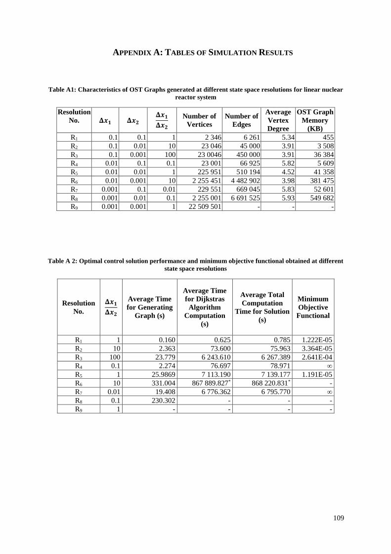
109

APPENDIX A: TABLES OF SIMULATION RESULTS

Table A1: Characteristics of OST Graphs generated at different state space resolutions for linear nuclear

reactor system

Resolution

No.

𝚫𝒙𝟏 𝚫𝒙𝟐 𝚫𝒙𝟏

𝚫𝒙𝟐

Number of

Vertices

Number of

Edges

Average

Vertex

Degree

OST Graph

Memory

(KB)

R1 0.1 0.1 1 2 346 6 261 5.34 455

R2 0.1 0.01 10 23 046 45 000 3.91 3 508

R3 0.1 0.001 100 23 0046 450 000 3.91 36 384

R4 0.01 0.1 0.1 23 001 66 925 5.82 5 609

R5 0.01 0.01 1 225 951 510 194 4.52 41 358

R6 0.01 0.001 10 2 255 451 4 482 902 3.98 381 475

R7 0.001 0.1 0.01 229 551 669 045 5.83 52 601

R8 0.001 0.01 0.1 2 255 001 6 691 525 5.93 549 682

R9 0.001 0.001 1 22 509 501 - - -

Table A 2: Optimal control solution performance and minimum objective functional obtained at different

state space resolutions

Resolution

No.

𝚫𝒙𝟏

𝚫𝒙𝟐

Average Time

for Generating

Graph (s)

Average Time

for Dijkstras

Algorithm

Computation

(s)

Average Total

Computation

Time for Solution

(s)

Minimum

Objective

Functional

R1 1 0.160 0.625 0.785 1.222E-05

R2 10 2.363 73.600 75.963 3.364E-05

R3 100 23.779 6 243.610 6 267.389 2.641E-04

R4 0.1 2.274 76.697 78.971 ∞

R5 1 25.9869 7 113.190 7 139.177 1.191E-05

R6 10 331.004 867 889.827* 868 220.831* -

R7 0.01 19.408 6 776.362 6 795.770 ∞

R8 0.1 230.302 - - -

R9 1 - - - -

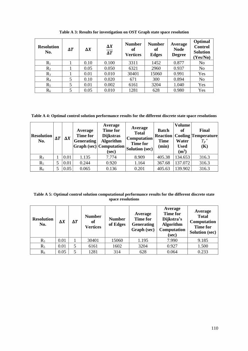
110

Table A 3: Results for investigation on OST Graph state space resolution

Resolution

No. 𝚫𝑻 𝚫𝑿

𝚫𝑿

𝚫𝑻

Number

of

Vertices

Number

of

Edges

Average

Node

Degree

Optimal

Control

Solution

(Yes/No)

R1 1 0.10 0.100 3311 1452 0.877 No

R2 1 0.05 0.050 6321 2960 0.937 No

R3 1 0.01 0.010 30401 15060 0.991 Yes

R4 5 0.10 0.020 671 300 0.894 No

R5 5 0.01 0.002 6161 3204 1.040 Yes

R6 5 0.05 0.010 1281 628 0.980 Yes

Table A 4: Optimal control solution performance results for the different discrete state space resolutions

Resolution

No. 𝚫𝑻 𝚫𝑿

Average

Time for

Generating

Graph (sec)

Average

Time for

Dijkstras

Algorithm

Computation

(sec)

Average

Total

Computation

Time for

Solution (sec)

Batch

Reaction

Time

(min)

Volume

of

Cooling

Water

Used

(m3)

Final

Temperature

𝑇𝐹∗

(K)

R3 1 0.01 1.135 7.774 8.909 405.38 134.653 316.3

R5 5 0.01 0.244 0.920 1.164 367.68 137.072 316.3

R6 5 0.05 0.065 0.136 0.201 405.63 139.902 316.3

Table A 5: Optimal control solution computational performance results for the different discrete state

space resolutions

Resolution

No. 𝚫𝑿 𝚫𝑻

Number

of

Vertices

Number

of Edges

Average

Time for

Generating

Graph (sec)

Average

Time for

Dijkstra’s

Algorithm

Computation

(sec)

Average

Total

Computation

Time for

Solution (sec)

R3 0.01 1 30401 15060 1.195 7.990 9.185

R5 0.01 5 6161 1602 3204 0.927 1.500

R6 0.05 5 1281 314 628 0.064 0.233