Package 'SpaDES.tools'

Package ‘SpaDES.tools’February 3, 2022

Type Package

Title Additional Tools for Developing Spatially Explicit DiscreteEvent Simulation (SpaDES) Models

Description Provides GIS and map utilities, plus additional modeling tools fordeveloping cellular automata, dynamic raster models, and agent based modelsin 'SpaDES'.Included are various methods for spatial spreading, spatial agents, GISoperations, random map generation, and others.See '?SpaDES.tools' for an categorized overview of these additional tools.

URL https://spades-tools.predictiveecology.org,

https://github.com/PredictiveEcology/SpaDES.tools

Date 2022-02-01

Version 0.3.10

Depends R (>= 4.0)

Imports backports, checkmate (>= 1.8.2), CircStats (>= 0.2-4),data.table (>= 1.10.4), fastmatch (>= 1.1-0), fpCompare (>=0.2.1), magrittr, methods, parallel, quickPlot, raster (>=2.5-8), Rcpp (>= 0.12.12), Require, rgeos, sp (>= 1.2-4), stats

Suggests animation, bit (>= 1.1-12), DBI, DEoptim (>= 2.2-4), dplyr,dqrng, fasterize, ff (>= 2.2-13), ffbase (>= 0.12.3),gdalUtils, googledrive, knitr, mgcv, RandomFields (>= 3.1.24),RColorBrewer (>= 1.1-2), rmarkdown, sf, testthat (>= 1.0.2),covr

Encoding UTF-8

Language en-CA

LinkingTo Rcpp

License GPL-3

BugReports https://github.com/PredictiveEcology/SpaDES.tools/issues

ByteCompile yes

1

https://spades-tools.predictiveecology.org


https://github.com/PredictiveEcology/SpaDES.tools/issues

2 R topics documented:

Collate 'RcppExports.R' 'heading.R' 'SELES.R''distanceFromEachPoint.R' 'environment.R' 'helpers.R''initialize.R' 'mapReduce.R' 'mergeRaster.R' 'movement.R''neighbourhood.R' 'numerical-comparisons.R' 'probability.R''resample.R' 'rings.R' 'spades-tools-deprecated.R''spades-tools-package.R' 'splitRaster.R' 'spread.R' 'spread2.R''spread3.R' 'studyArea.R' 'zzz.R'

RoxygenNote 7.1.2

NeedsCompilation yes

Author Alex M Chubaty [aut, cre] (<https://orcid.org/0000-0001-7146-8135>),Eliot J B McIntire [aut] (<https://orcid.org/0000-0002-6914-8316>),Yong Luo [ctb],Steve Cumming [ctb],Jean Marchal [ctb],Her Majesty the Queen in Right of Canada, as represented by theMinister of Natural Resources Canada [cph]

Maintainer Alex M Chubaty <[email protected]>

Repository CRAN

Date/Publication 2022-02-03 07:50:13 UTC

R topics documented:SpaDES.tools-package . . . . . . . . . . . . . . . . . . . . . . . . . . . . . . . . . . . 3.pointDistance . . . . . . . . . . . . . . . . . . . . . . . . . . . . . . . . . . . . . . . . 5adj . . . . . . . . . . . . . . . . . . . . . . . . . . . . . . . . . . . . . . . . . . . . . . 6agentLocation . . . . . . . . . . . . . . . . . . . . . . . . . . . . . . . . . . . . . . . . 8cir . . . . . . . . . . . . . . . . . . . . . . . . . . . . . . . . . . . . . . . . . . . . . . 9cirSpecialQuick . . . . . . . . . . . . . . . . . . . . . . . . . . . . . . . . . . . . . . . 12distanceFromEachPoint . . . . . . . . . . . . . . . . . . . . . . . . . . . . . . . . . . . 13duplicatedInt . . . . . . . . . . . . . . . . . . . . . . . . . . . . . . . . . . . . . . . . 16dwrpnorm2 . . . . . . . . . . . . . . . . . . . . . . . . . . . . . . . . . . . . . . . . . 17fastCrop . . . . . . . . . . . . . . . . . . . . . . . . . . . . . . . . . . . . . . . . . . . 18gaussMap . . . . . . . . . . . . . . . . . . . . . . . . . . . . . . . . . . . . . . . . . . 18heading . . . . . . . . . . . . . . . . . . . . . . . . . . . . . . . . . . . . . . . . . . . 20initiateAgents . . . . . . . . . . . . . . . . . . . . . . . . . . . . . . . . . . . . . . . . 21inRange . . . . . . . . . . . . . . . . . . . . . . . . . . . . . . . . . . . . . . . . . . . 23mergeRaster . . . . . . . . . . . . . . . . . . . . . . . . . . . . . . . . . . . . . . . . . 24middlePixel . . . . . . . . . . . . . . . . . . . . . . . . . . . . . . . . . . . . . . . . . 27move . . . . . . . . . . . . . . . . . . . . . . . . . . . . . . . . . . . . . . . . . . . . . 27numAgents . . . . . . . . . . . . . . . . . . . . . . . . . . . . . . . . . . . . . . . . . 29patchSize . . . . . . . . . . . . . . . . . . . . . . . . . . . . . . . . . . . . . . . . . . 29probInit . . . . . . . . . . . . . . . . . . . . . . . . . . . . . . . . . . . . . . . . . . . 30randomPolygons . . . . . . . . . . . . . . . . . . . . . . . . . . . . . . . . . . . . . . 31randomStudyArea . . . . . . . . . . . . . . . . . . . . . . . . . . . . . . . . . . . . . . 32rasterizeReduced . . . . . . . . . . . . . . . . . . . . . . . . . . . . . . . . . . . . . . 33rings . . . . . . . . . . . . . . . . . . . . . . . . . . . . . . . . . . . . . . . . . . . . . 34

https://orcid.org/0000-0001-7146-8135

https://orcid.org/0000-0002-6914-8316

SpaDES.tools-package 3

runifC . . . . . . . . . . . . . . . . . . . . . . . . . . . . . . . . . . . . . . . . . . . . 37specificNumPerPatch . . . . . . . . . . . . . . . . . . . . . . . . . . . . . . . . . . . . 37spokes . . . . . . . . . . . . . . . . . . . . . . . . . . . . . . . . . . . . . . . . . . . . 38spread . . . . . . . . . . . . . . . . . . . . . . . . . . . . . . . . . . . . . . . . . . . . 41spread2 . . . . . . . . . . . . . . . . . . . . . . . . . . . . . . . . . . . . . . . . . . . 52spread3 . . . . . . . . . . . . . . . . . . . . . . . . . . . . . . . . . . . . . . . . . . . 60testEquivalentMetadata . . . . . . . . . . . . . . . . . . . . . . . . . . . . . . . . . . . 64transitions . . . . . . . . . . . . . . . . . . . . . . . . . . . . . . . . . . . . . . . . . . 65wrap . . . . . . . . . . . . . . . . . . . . . . . . . . . . . . . . . . . . . . . . . . . . . 66

Index 68

SpaDES.tools-package Categorized overview of the SpaDES.tools package

Description

1 Spatial spreading/distances methods

Spatial contagion is a key phenomenon for spatially explicit simulation models. Contagion can bemodelled using discrete approaches or continuous approaches. Several functions assist with these:

adj An optimized (i.e., faster) version of adjacentcir Identify pixels in a circle around a SpatialPoints* objectdirectionFromEachPoint Fast calculation of direction and distance surfacesdistanceFromEachPoint Fast calculation of distance surfacesrings Identify rings around focal cells (e.g., buffers and donuts)spokes TO DO: need descriptionspread Contagious cellular automatawrap Create a torus from a grid

2 Spatial agent methods

Agents have several methods and functions specific to them:

crw Simple correlated random walk functionheading Determines the heading between SpatialPoints*makeLines Makes SpatialLines object for, e.g., drawing arrowsmove A meta function that can currently only take "crw"specificNumPerPatch Initiate a specific number of agents per patch

4 SpaDES.tools-package

3 GIS operations

In addition to the vast amount of GIS operations available in R (mostly from contributed pack-ages such as sp, raster, maps, maptools and many others), we provide the following GIS-relatedfunctions:

equalExtent Assess whether a list of extents are all equal

4 Map-reduce - type operations

These functions convert between reduced and mapped representations of the same data. This al-lows compact representation of, e.g., rasters that have many individual pixels that share identicalinformation.

rasterizeReduced Convert reduced representation to full raster

5 Random Map Generation

It is often useful to build dummy maps with which to build simulation models before all data areavailable. These dummy maps can later be replaced with actual data maps.

gaussMap Creates a random map using Gaussian random fieldsrandomPolygons Creates a random polygon with specified number of classes

6 SELES-type approach to simulation

These functions are essentially skeletons and are not fully implemented. They are intended to maketranslations from SELES. You must know how to use SELES for these to be useful:

agentLocation Agent locationinitiateAgents Initiate agents into a SpatialPointsDataFramenumAgents Number of agentsprobInit Probability of initiating an agent or eventtransitions Transition probability

7 Package options

SpaDES packages use the following options to configure behaviour:

• spades.lowMemory: If true, some functions will use more memory efficient (but slower)algorithms. Default FALSE.

Author(s)

Maintainer: Alex M Chubaty <[email protected]> (ORCID)

Authors:

http://www.gowlland.ca/

https://orcid.org/0000-0001-7146-8135

.pointDistance 5

• Eliot J B McIntire <[email protected]> (ORCID)

Other contributors:

• Yong Luo <[email protected]> [contributor]

• Steve Cumming <[email protected]> [contributor]

• Jean Marchal <[email protected]> [contributor]

• Her Majesty the Queen in Right of Canada, as represented by the Minister of Natural Re-sources Canada [copyright holder]

See Also

Useful links:

• https://spades-tools.predictiveecology.org

• https://github.com/PredictiveEcology/SpaDES.tools

• Report bugs at https://github.com/PredictiveEcology/SpaDES.tools/issues

.pointDistance Alternative point distance (and direction) calculations

Description

These have been written with speed in mind.

Usage

.pointDistance(from,to,angles = NA,maxDistance = NA_real_,otherFromCols = FALSE

)

Arguments

from TODO: description needed

to TODO: description needed

angles TODO: description needed

maxDistance TODO: description needed

otherFromCols TODO: description needed

https://orcid.org/0000-0002-6914-8316

https://spades-tools.predictiveecology.org


https://github.com/PredictiveEcology/SpaDES.tools/issues

6 adj

adj Fast ‘adjacent‘ function, and Just In Time compiled version

Description

Faster function for determining the cells of the 4, 8 or bishop neighbours of the cells. This is ahybrid function that uses matrix for small numbers of loci (<1e4) and data.table for larger numbersof loci

Usage

adj(x = NULL,cells,directions = 8,sort = FALSE,pairs = TRUE,include = FALSE,target = NULL,numCol = NULL,numCell = NULL,match.adjacent = FALSE,cutoff.for.data.table = 2000,torus = FALSE,id = NULL,numNeighs = NULL,returnDT = FALSE

)

Arguments

x Raster* object for which adjacency will be calculated.

cells vector of cell numbers for which adjacent cells should be found. Cell numbersstart with 1 in the upper-left corner and increase from left to right and from topto bottom.

directions the number of directions in which cells should be connected: 4 (rook’s case), 8(queen’s case), or "bishop" to connect cells with one-cell diagonal moves. Ora neighbourhood matrix (see Details).

sort logical. Whether the outputs should be sorted or not, using cell ids of the fromcells (and to cells, if match.adjacent is TRUE).

pairs logical. If TRUE, a matrix of pairs of adjacent cells is returned. If FALSE, a vectorof cells adjacent to cells is returned

include logical. Should the focal cells be included in the result?

target a vector of cells that can be spread to. This is the inverse of a mask.

adj 7

numCol numeric indicating number of columns in the raster. Using this with numCell isa bit faster execution time.

numCell numeric indicating number of cells in the raster. Using this with numCol is a bitfaster execution time.

match.adjacent logical. Should the returned object be the same as raster::adjacent. DefaultFALSE, which is faster.

cutoff.for.data.table

numeric. If the number of cells is above this value, the function uses data.tablewhich is faster with large numbers of cells. Default is 5000, which appears tobe the turning point where data.table becomes faster.

torus Logical. Should the spread event wrap around to the other side of the raster?Default is FALSE.

id numeric If not NULL (default), then function will return "id" column.

numNeighs A numeric scalar, indicating how many neighbours to return. Must be less thanor equal to directions; which neighbours are random with equal probabilities.

returnDT A logical. If TRUE, then the function will return the result as a data.table, ifthe internals used data.table, i.e., if number of cells is greater than cutoff.for.data.table.User should be warned that this will therefore cause the output format to changedepending cutoff.for.data.table. This will be faster for situations wherecutoff.for.data.table = TRUE.

Details

Between 4x (large number loci) to 200x (small number loci) speed gains over adjacent in rasterpackage. There is some extra speed gain if NumCol and NumCells are passed rather than a raster.Efficiency gains come from: 1. use data.table internally - no need to remove NAs becausewrapped or outside points are just removed directly with data.table - use data.table to sort and fastselect (though not fastest possible) 2. don’t make intermediate objects; just put calculation intoreturn statement

The steps used in the algorithm are: 1. Calculate indices of neighbouring cells 2. Remove "to" cellsthat are - <1 or >numCells (i.e., they are above or below raster), using a single modulo calculation- where the modulo of "to" cells is equal to 1 if "from" cells are 0 (wrapped right to left) - or wherethe modulo of the "to" cells is equal to 0 if "from" cells are 1 (wrapped left to right)

Value

Either a matrix (if more than 1 column, i.e., pairs = TRUE, and/or id is provided), a vector (ifonly one column), or a data.table (if cutoff.for.data.table is less than length(cells) andreturnDT is TRUE. To get a consistent output, say a matrix, it would be wise to test the output forits class. The variable output is done to minimize coercion to maintain speed. The columns will beone or more of id, from, to.

Author(s)

Eliot McIntire

8 agentLocation

See Also

adjacent

Examples

library(raster)a <- raster(extent(0, 1000, 0, 1000), res = 1)sam <- sample(1:length(a), 1e4)numCol <- ncol(a)numCell <- ncell(a)adj.new <- adj(numCol = numCol, numCell = numCell, cells = sam, directions = 8)adj.new <- adj(numCol = numCol, numCell = numCell, cells = sam, directions = 8,

include = TRUE)

agentLocation SELES - Agent Location at initiation

Description

Sets the the location of the initiating agents. NOT YET FULLY IMPLEMENTED.

A SELES-like function to maintain conceptual backwards compatibility with that simulation tool.This is intended to ease transitions from SELES.

You must know how to use SELES for these to be useful.

Usage

agentLocation(map)

Arguments

map A SpatialPoints*, SpatialPolygons*, or Raster* object.

Value

Object of same class as provided as input. If a Raster*, then zeros are converted to NA.

Author(s)

Eliot McIntire


cir 9

cir Identify pixels in a circle or ring (donut) around an object.

Description

Identify the pixels and coordinates that are at a (set of) buffer distance(s) of the objects passedinto coords. This is similar to rgeos::gBuffer but much faster and without the geo referencinginformation. In other words, it can be used for similar problems, but where speed is important. Thiscode is substantially adapted from PlotRegionHighlighter::createCircle.

Usage

cir(landscape,coords,loci,maxRadius = ncol(landscape)/4,minRadius = maxRadius,allowOverlap = TRUE,allowDuplicates = FALSE,includeBehavior = "includePixels",returnDistances = FALSE,angles = NA_real_,returnAngles = FALSE,returnIndices = TRUE,closest = FALSE,simplify = TRUE

)

Arguments

landscape Raster on which the circles are built.

coords Either a matrix with 2 (or 3) columns, x and y (and id), representing the coordi-nates (and an associated id, like cell index), or a SpatialPoints* object aroundwhich to make circles. Must be same coordinate system as the landscape argu-ment. Default is missing, meaning it uses the default to loci

loci Numeric. An alternative to coords. These are the indices on landscape toinitiate this function. See coords. Default is one point in centre of landscape..

maxRadius Numeric vector of length 1 or same length as coords

minRadius Numeric vector of length 1 or same length as coords. Default is maxRadius,meaning return all cells that are touched by the narrow ring at that exact radius.If smaller than maxRadius, then this will create a buffer or donut or ring.

allowOverlap Logical. Should duplicates across id be removed or kept. Default TRUE.

10 cir

allowDuplicates

Logical. Should duplicates within id be removed or kept. Default FALSE. Thisis useful if the actual x, y coordinates are desired, rather than the cell indices.This will increase the size of the returned object.

includeBehavior

Character string. Currently accepts only "includePixels", the default, and "ex-cludePixels". See details.

returnDistances

Logical. If TRUE, then a column will be added to the returned data.table thatreports the distance from coords to every point that was in the circle/donutsurrounding coords. Default FALSE, which is faster.

angles Numeric. Optional vector of angles, in radians, to use. This will create "spokes"outward from coords. Default is NA, meaning, use internally derived angles thatwill "fill" the circle.

returnAngles Logical. If TRUE, then a column will be added to the returned data.table thatreports the angle from coords to every point that was in the circle/donut sur-rounding coords. Default FALSE.

returnIndices Logical or numeric. If 1 or TRUE, will return a data.table with indices andvalues of successful spread events. If 2, it will simply return a vector of pixelindices of all cells that were touched. This will be the fastest option. If FALSE,then it will return a raster with values. See Details.

closest Logical. When determining non-overlapping circles, should the function givepreference to the closest loci or the first one (much faster). Default is FALSE,meaning the faster, though maybe not desired behaviour.

simplify logical. If TRUE, then all duplicate pixels are removed. This means that somex, y combinations will disappear.

Details

This function identifies all the pixels as defined by a donut with inner radius minRadius and outerradius of maxRadius. The includeBehavior defines whether the cells that intersect the radii butwhose centres are not inside the donut are included includePixels or not excludePixels in thereturned pixels identified. If this is excludePixels, and if a minRadius and maxRadius are equal,this will return no pixels.

Value

A matrix with 4 columns, id, indices, x, y. The x and y indicate the exact coordinates of theindices (i.e., cell number) of the landscape associated with the ring or circle being identified bythis function.

See Also

rings which uses spread internally. cir tends to be faster when there are few starting points,rings tends to be faster when there are many starting points. cir scales with maxRadius ^ 2 andcoords. Another difference between the two functions is that rings takes the centre of the pixel asthe centre of a circle, whereas cir takes the exact coordinates. See example. For the specific case ofcreating distance surfaces from specific points, see distanceFromEachPoint, which is often faster.For the more general GIS buffering, see rgeos::gBuffer.

cir 11

Examples

library(data.table)library(sp)library(raster)library(quickPlot)

set.seed(1462)

if (require(RandomFields)) {# circle centredras <- raster(extent(0, 15, 0, 15), res = 1, val = 0)middleCircle <- cir(ras)ras[middleCircle[, "indices"]] <- 1circlePoints <- SpatialPoints(middleCircle[, c("x", "y")])if (interactive()) {clearPlot()Plot(ras)Plot(circlePoints, addTo = "ras")

}

# circles non centredras <- randomPolygons(ras, numTypes = 4)n <- 2agent <- SpatialPoints(coords = cbind(x = stats::runif(n, xmin(ras), xmax(ras)),

y = stats::runif(n, xmin(ras), xmax(ras))))

cirs <- cir(ras, agent, maxRadius = 15, simplify = TRUE) ## TODO: empty with some seeds! e.g. 1642cirsSP <- SpatialPoints(coords = cirs[, c("x", "y")]) ## TODO: error with some seeds! e.g. 1642cirsRas <- raster(ras)cirsRas[] <- 0cirsRas[cirs[, "indices"]] <- 1

if (interactive()) {clearPlot()Plot(ras)Plot(cirsRas, addTo = "ras", cols = c("transparent", "#00000055"))Plot(agent, addTo = "ras")Plot(cirsSP, addTo = "ras")

}

# Example comparing rings and cira <- raster(extent(0, 30, 0, 30), res = 1)hab <- gaussMap(a, speedup = 1) # if raster is large (>1e6 pixels) use speedup > 1radius <- 4n <- 2coords <- SpatialPoints(coords = cbind(x = stats::runif(n, xmin(hab), xmax(hab)),

y = stats::runif(n, xmin(hab), xmax(hab))))

# cirscirs <- cir(hab, coords, maxRadius = rep(radius, length(coords)), simplify = TRUE)

# rings

12 cirSpecialQuick

loci <- cellFromXY(hab, coordinates(coords))cirs2 <- rings(hab, loci, maxRadius = radius, minRadius = radius - 1, returnIndices = TRUE)

# Plot bothras1 <- raster(hab)ras1[] <- 0ras1[cirs[, "indices"]] <- cirs[, "id"]

ras2 <- raster(hab)ras2[] <- 0ras2[cirs2$indices] <- cirs2$idif (interactive()) {

clearPlot()Plot(ras1, ras2)

}

a <- raster(extent(0, 100, 0, 100), res = 1)hab <- gaussMap(a, speedup = 1)cirs <- cir(hab, coords, maxRadius = 44, minRadius = 0)ras1 <- raster(hab)ras1[] <- 0cirsOverlap <- data.table(cirs)[, list(sumIDs = sum(id)), by = indices]ras1[cirsOverlap$indices] <- cirsOverlap$sumIDsif (interactive()) {

clearPlot()Plot(ras1)

}

# Provide a specific set of anglesras <- raster(extent(0, 330, 0, 330), res = 1)ras[] <- 0n <- 2coords <- cbind(x = stats::runif(n, xmin(ras), xmax(ras)),

y = stats::runif(n, xmin(ras), xmax(ras)))circ <- cir(ras, coords, angles = seq(0, 2 * pi, length.out = 21),

maxRadius = 200, minRadius = 0, returnIndices = FALSE,allowOverlap = TRUE, returnAngles = TRUE)

}

cirSpecialQuick This is a very fast version of cir with allowOverlap= TRUE, allowDuplicates = FALSE, returnIndices =TRUE, returnDistances = TRUE, and includeBehavior ="excludePixels". It is used inside spread2, when asymmetryis active. The basic algorithm is to run cir just once, then add to thex,y coordinates of every locus.

Description

This is a very fast version of cir with allowOverlap = TRUE, allowDuplicates = FALSE, returnIndices= TRUE, returnDistances = TRUE, and includeBehavior = "excludePixels". It is used inside

distanceFromEachPoint 13

spread2, when asymmetry is active. The basic algorithm is to run cir just once, then add to thex,y coordinates of every locus.

Usage

.cirSpecialQuick(landscape, loci, maxRadius, minRadius)

Arguments





distanceFromEachPoint Calculate distances and directions between many points and manygrid cells

Description

This is a modification of distanceFromPoints for the case of many points. This version can of-ten be faster for a single point because it does not return a RasterLayer. This is different thandistanceFromPoints because it does not take the minimum distance from the set of points to allcells. Rather this returns the every pair-wise point distance. As a result, this can be used for doinginverse distance weightings, seed rain, cumulative effects of distance-based processes etc. If mem-ory limitation is an issue, maxDistance will keep memory use down, but with the consequences thatthere will be a maximum distance returned. This function has the potential to use a lot of memoryif there are a lot of from and to points.

Usage

distanceFromEachPoint(from,to = NULL,landscape,angles = NA_real_,maxDistance = NA_real_,cumulativeFn = NULL,distFn = function(dist) 1/(1 + dist),cl,...

)

14 distanceFromEachPoint

Arguments

from Numeric matrix with 2 or 3 or more columns. They must include x and y, rep-resenting x and y coordinates of "from" cell. If there is a column named "id",it will be "id" from to, i.e,. specific pair distances. All other columns will beincluded in the return value of the function.

to Numeric matrix with 2 or 3 columns (or optionally more, all of which will bereturned), x and y, representing x and y coordinates of "to" cells, and optional"id" which will be matched with "id" from from. Default is all cells.

landscape RasterLayer. optional. This is only used if to is NULL, in which case all cellsare considered to.

angles Logical. If TRUE, then the function will return angles in radians, as well asdistances.

maxDistance Numeric in units of number of cells. The algorithm will build the whole surface(from from to to), but will remove all distances that are above this distance.Using this will keep memory use down.

cumulativeFn A function that can be used to incrementally accumulate values in each to loca-tion, as the function iterates through each from. See Details.

distFn A function. This can be a function of landscape, fromCell (single integervalue of a from pixel), toCells (integer vector value of all the to pixel indices),and dist. If cumulativeFn is supplied, this will be used to convert the distancesto some other set of units that will be accumulated by the cumulativeFn. SeeDetails and examples.

cl A cluster object. Optional. This would generally be created using parallel::makeClusteror equivalent. This is an alternative way, instead of beginCluster(), to use par-allelism for this function, allowing for more control over cluster use.

... Any additional objects needed for distFn.

Details

This function is cluster aware. If there is a cluster running, it will use it. To start a cluster usebeginCluster, with N being the number of cores to use. See examples in SpaDES.core::experiment.

If the user requires an id (indicating the from cell for each to cell) to be returned with the function,the user must add an identifier to the from matrix, such as "id". Otherwise, the function will onlyreturn the coordinates and distances.

distanceFromEachPoint calls .pointDistance, which is not intended to be called directly by theuser.

This function has the potential to return a very large object, as it is doing pairwise distances (andoptionally directions) between from and to. If there are memory limitations because there aremany from and many to points, then cumulativeFn and distFn can be used. These two functionstogether will be used iteratively through the from points. The distFn should be a transformationof distances to be used by the cumulativeFn function. For example, if distFn is 1 / (1+x), thedefault, and cumulativeFn is `+`, then it will do a sum of inverse distance weights. See examples.

distanceFromEachPoint 15

Value

A sorted matrix on id with same number of rows as to, but with one extra column, "dists",indicating the distance between from and to.

See Also

rings, cir, distanceFromPoints, which can all be made to do the same thing, under specificcombinations of arguments. But each has different primary use cases. Each is also faster underdifferent conditions. For instance, if maxDistance is relatively small compared to the number ofcells in the landscape, then cir will likely be faster. If a minimum distance from all cells in thelandscape to any cell in from, then distanceFromPoints will be fastest. This function scales bestwhen there are many to points or all cells are used to = NULL (which is default).

Examples

library(raster)library(quickPlot)

n <- 2distRas <- raster(extent(0, 40, 0, 40), res = 1)coords <- cbind(x = round(runif(n, xmin(distRas), xmax(distRas))) + 0.5,

y = round(runif(n, xmin(distRas), xmax(distRas))) + 0.5)

# inverse distance weightsdists1 <- distanceFromEachPoint(coords, landscape = distRas)indices <- cellFromXY(distRas, dists1[, c("x", "y")])invDist <- tapply(dists1[, "dists"], indices, function(x) sum(1 / (1 + x))) # idw functiondistRas[] <- as.vector(invDist)if (interactive()) {

clearPlot()Plot(distRas)

}

# With iterative summing via cumulativeFn to keep memory use low, with same resultdists1 <- distanceFromEachPoint(coords[, c("x", "y"), drop = FALSE],

landscape = distRas, cumulativeFn = `+`)idwRaster <- raster(distRas)idwRaster[] <- dists1[, "dists"]if (interactive()) Plot(idwRaster)

all(idwRaster[] == distRas[]) # TRUE

# A more complex example of cumulative inverse distance sums, weighted by the value# of the origin cellras <- raster(extent(0, 34, 0, 34), res = 1, val = 0)rp <- randomPolygons(ras, numTypes = 10) ^ 2n <- 15cells <- sample(ncell(ras), n)coords <- xyFromCell(ras, cells)distFn <- function(landscape, fromCell, dist) landscape[fromCell] / (1 + dist)

16 duplicatedInt

#beginCluster(3) # can do paralleldists1 <- distanceFromEachPoint(coords[, c("x", "y"), drop = FALSE],

landscape = rp, distFn = distFn, cumulativeFn = `+`)#endCluster() # if beginCluster was run

idwRaster <- raster(ras)idwRaster[] <- dists1[, "dists"]if (interactive()) {

clearPlot()Plot(rp, idwRaster)sp1 <- SpatialPoints(coords)Plot(sp1, addTo = "rp")Plot(sp1, addTo = "idwRaster")

}

# On linux; can use numeric passed to cl; will use mclapply with mc.cores = clif (identical(Sys.info()["sysname"], "Linux")) {

dists1 <- distanceFromEachPoint(coords[, c("x", "y"), drop = FALSE],landscape = rp, distFn = distFn,cumulativeFn = `+`, cl = 2)

}

duplicatedInt Rcpp duplicated on integers using Rcpp Sugar

Description

.duplicatedInt does same as duplicated in R, but only on integers, and faster. It uses Rcppsugar

Usage

duplicatedInt(x)

Arguments

x Integer Vector

Value

A logical vector, as per duplicated

dwrpnorm2 17

dwrpnorm2 Vectorized wrapped normal density function

Description

This is a modified version of dwrpnorm found in CircStats to allow for multiple angles at once(i.e., vectorized on theta and mu).

Usage

dwrpnorm2(theta, mu, rho, sd = 1, acc = 1e-05, tol = acc)

Arguments

theta value at which to evaluate the density function, measured in radians.

mu mean direction of distribution, measured in radians.

rho mean resultant length of distribution.

sd different way of select rho, see details below.

acc parameter defining the accuracy of the estimation of the density. Terms areadded to the infinite summation that defines the density function until successiveestimates are within acc of each other.

tol the same as acc.

Author(s)

Eliot McIntire

Examples

# Values for which to evaluate densitytheta <- c(1:500) * 2 * pi / 500# Compute wrapped normal density functiondensity <- c(1:500)for(i in 1:500) density[i] <- dwrpnorm2(theta[i], pi, .75)if (interactive()) plot(theta, density)# Approximate area under density curvesum(density * 2 * pi / 500)

18 gaussMap

fastCrop fastCrop is a wrapper around velox::VeloxRaster_crop, thoughraster::crop is faster under many tests.

Description

fastCrop is a wrapper around velox::VeloxRaster_crop, though raster::crop is faster undermany tests.

Usage

fastCrop(x, y, ...)

Arguments

x Raster to crop

y Extent object, or any object from which an Extent object can be extracted (seeDetails)

... Additional arguments as for writeRaster

See Also

velox::VeloxRaster_crop

gaussMap Produce a raster of a random Gaussian process.

Description

This is a wrapper for the RFsimulate function in the RandomFields package. The main addition isthe speedup argument which allows for faster map generation. A speedup of 1 is normal and willget progressively faster as the number increases, at the expense of coarser pixel resolution of thepattern generated.

Usage

gaussMap(x,scale = 10,var = 1,speedup = 1,method = "RMexp",alpha = 1,inMemory = FALSE,...

)

gaussMap 19

Arguments

x A spatial object (e.g., a RasterLayer).

scale The spatial scale in map units of the Gaussian pattern.

var Spatial variance.

speedup An numeric value indicating how much faster than ’normal’ to generate maps.It may be necessary to give a value larger than 1 for large maps. Default is 1.

method The type of model used to produce the Gaussian pattern. Should be one of"RMgauss" (Gaussian covariance model), "RMstable" (the stable powered ex-ponential model), or the default, "RMexp" (exponential covariance model).

alpha A required parameter of the ’RMstable’ model. Should be in the interval [0,2]to provide a valid covariance function. Default is 1.

inMemory Should the RasterLayer be forced to be in memory? Default FALSE.

... Additional arguments to raster.

Value

A raster map with same extent as x, with a Gaussian random pattern.

See Also

RFsimulate and extent

Examples

## Not run:if (require(RandomFields)) {

library(raster)nx <- ny <- 100Lr <- raster(nrows = ny, ncols = nx, xmn = -nx/2, xmx = nx/2, ymn = -ny/2, ymx = ny/2)speedup <- max(1, nx/5e2)map1 <- gaussMap(r, scale = 300, var = 0.03, speedup = speedup, inMemory = TRUE)if (interactive()) Plot(map1)

# with non-default methodmap1 <- gaussMap(r, scale = 300, var = 0.03, method = "RMgauss")

}

## End(Not run)

20 heading

heading Heading between spatial points.

Description

Determines the heading between spatial points.

Usage

heading(from, to)

## S4 method for signature 'SpatialPoints,SpatialPoints'heading(from, to)

## S4 method for signature 'matrix,matrix'heading(from, to)

## S4 method for signature 'matrix,SpatialPoints'heading(from, to)

## S4 method for signature 'SpatialPoints,matrix'heading(from, to)

Arguments

from The starting position; an object of class SpatialPoints.

to The ending position; an object of class SpatialPoints.

Value

The heading between the points, in degrees.

Author(s)

Eliot McIntire

Examples

library(sp)N <- 10L # number of agentsx1 <- stats::runif(N, -50, 50) # previous X locationy1 <- stats::runif(N, -50, 50) # previous Y locationx0 <- stats::rnorm(N, x1, 5) # current X locationy0 <- stats::rnorm(N, y1, 5) # current Y location

# using SpatialPointsprev <- SpatialPoints(cbind(x = x1, y = y1))curr <- SpatialPoints(cbind(x = x0, y = y0))

initiateAgents 21

heading(prev, curr)

# using matrixprev <- matrix(c(x1, y1), ncol = 2, dimnames = list(NULL, c("x","y")))curr <- matrix(c(x0, y0), ncol = 2, dimnames = list(NULL, c("x","y")))heading(prev, curr)

#using bothprev <- SpatialPoints(cbind(x = x1, y = y1))curr <- matrix(c(x0, y0), ncol = 2, dimnames = list(NULL, c("x","y")))heading(prev, curr)

prev <- matrix(c(x1, y1), ncol = 2, dimnames = list(NULL, c("x","y")))curr <- SpatialPoints(cbind(x = x0, y = y0))heading(prev, curr)

initiateAgents SELES - Initiate agents

Description

Sets the the number of agents to initiate. THIS IS NOT FULLY IMPLEMENTED.



Usage

initiateAgents(map, numAgents, probInit, asSpatialPoints = TRUE, indices)

## S4 method for signature 'Raster,missing,missing,ANY,missing'initiateAgents(map, numAgents, probInit, asSpatialPoints)

## S4 method for signature 'Raster,missing,Raster,ANY,missing'initiateAgents(map, probInit, asSpatialPoints)

## S4 method for signature 'Raster,numeric,missing,ANY,missing'initiateAgents(map, numAgents, probInit, asSpatialPoints = TRUE, indices)

## S4 method for signature 'Raster,numeric,Raster,ANY,missing'initiateAgents(map, numAgents, probInit, asSpatialPoints)

## S4 method for signature 'Raster,missing,missing,ANY,numeric'initiateAgents(map, numAgents, probInit, asSpatialPoints = TRUE, indices)


22 initiateAgents

Arguments

map RasterLayer with extent and resolution of desired return object

numAgents numeric resulting from a call to numAgents

probInit a Raster resulting from a probInit callasSpatialPoints

logical. Should returned object be RasterLayer or SpatialPointsDataFrame(default)

indices numeric. Indices of where agents should start

Value

A SpatialPointsDataFrame, with each row representing an individual agent

Author(s)

Eliot McIntire

Examples

if (require(RandomFields)) {library(magrittr)library(raster)library(quickPlot)

map <- raster(xmn = 0, xmx = 10, ymn = 0, ymx = 10, val = 0, res = 1)map <- gaussMap(map, scale = 1, var = 4, speedup = 1)pr <- probInit(map, p = (map/maxValue(map))^2)agents <- initiateAgents(map, 100, pr)if (interactive()) {

clearPlot()Plot(map)Plot(agents, addTo = "map")

}# Test that they are indeed selecting according to probabilities in prlibrary(data.table)dt1 <- data.table(table(round(map[agents], 0)))setnames(dt1, old = "N", new = "count")dt2 <- data.table(table(round(map[], 0)))setnames(dt2, old = "N", new = "available")dt <-dt1[dt2, on = "V1"] # join the counts and available data.tablessetnames(dt, old = "V1", new = "mapValue")dt[, selection := count/available]dt[is.na(selection), selection := 0]if (interactive())

with(dt, {plot(mapValue, selection)})#'# Note, can also produce a Raster representing agents,# then the number of points produced can't be more than# the number of pixels:agentsRas <- initiateAgents(map, 30, pr, asSpatialPoints = FALSE)

inRange 23

if (interactive()) Plot(agentsRas)#'if (require(dplyr) && getRversion() >= 3.4) {

# Check that the agents are more often at the higher probability areas based on prif (utils::packageVersion("raster") >= "2.8-11") {out <- data.frame(stats::na.omit(crosstab(agentsRas, map)), table(round(map[]))) %>%

dplyr::mutate(selectionRatio = Freq / Freq.1) %>%dplyr::select(-layer.1, -Var1) %>%dplyr::rename(Present = Freq, Avail = Freq.1, Type = layer.2)

} else {out <- data.frame(stats::na.omit(crosstab(agentsRas, map)), table(round(map[]))) %>%

dplyr::mutate(selectionRatio = Freq/Freq.1) %>%dplyr::select(-Var1, -Var1.1) %>%dplyr::rename(Present = Freq, Avail = Freq.1, Type = Var2)

}out

}}

inRange Test whether a number lies within range [a,b]

Description

Default values of a=0; b=1 allow for quick test if x is a probability.

Usage

inRange(x, a = 0, b = 1)

Arguments

x values to be testeda lower bound (default 0)b upper bound (default 1)

Value

Logical vectors. NA values in x are retained.

Author(s)

Alex Chubaty

Examples

set.seed(100)x <- stats::rnorm(4) # -0.50219235 0.13153117 -0.07891709 0.88678481inRange(x, 0, 1)

24 mergeRaster

mergeRaster Split and re-merge RasterLayer(s)

Description

splitRaster divides up a raster into an arbitrary number of pieces (tiles). Split rasters can berecombined using do.call(merge,y) or mergeRaster(y), where y <-splitRaster(x).

Usage

mergeRaster(x, fun = NULL)

## S4 method for signature 'list'mergeRaster(x, fun = NULL)

splitRaster(r,nx = 1,ny = 1,buffer = c(0, 0),path = NA,cl,rType = "FLT4S",fExt = ".grd"

)

## S4 method for signature 'RasterLayer'splitRaster(r,nx = 1,ny = 1,buffer = c(0, 0),path = NA,cl,rType = "FLT4S",fExt = ".grd"

)

Arguments

x A list of split raster tiles (i.e., from splitRaster).

fun Function (e.g. mean, min, or max that accepts a na.rm argument. The default ismean.

r The raster to be split.

nx The number of tiles to make along the x-axis.

ny The number of tiles to make along the y-axis.

mergeRaster 25

buffer Numeric vector of length 2 giving the size of the buffer along the x and y axes.If these values less than or equal to 1 are used, this is interpreted as the numberof pixels (cells) to use as a buffer. Values between 0 and 1 are interpreted asproportions of the number of pixels in each tile (rounded up to an integer value).Default is c(0,0), which means no buffer.

path Character specifying the directory to which the split tiles will be saved. If miss-ing, the function will write to memory.

cl A cluster object. Optional. This would generally be created using parallel::makeClusteror equivalent. This is an alternative way, instead of beginCluster(), to use par-allelism for this function, allowing for more control over cluster use.

rType Data type of the split rasters. Defaults to FLT4S.

fExt file extension (e.g., ".grd" or ".tif") specifying the file format.

Details

mergeRaster differs from merge in how overlapping tile regions are handled: merge retains thevalues of the first raster in the list. This has the consequence of retaining the values from thebuffered region in the first tile in place of the values from the neighbouring tile. On the other hand,mergeRaster retains the values of the tile region, over the values in any buffered regions. This isuseful for reducing edge effects when performing raster operations involving contagious processes.To use the average of cell values, or do another computation, use mosaic. mergeRaster is alsofaster than merge. mergeRaster also differs from mosaic in speed and ability to take a raster list.It can, however, use the average of cell values, or do other computations. At last, mergeRastercan also merge tiles of a split raster that were resampled and, therefore, could have had differentchanges in the buffer sizes on each side of the raster. If the user resamples the tiles and the newresolution is not a multiple of the original one, mergeRaster will use mosaic with the max functionto merge the tiles with a message. The user can also pass the function to be used when mosaic istriggered.

This function is parallel-aware, using the same mechanism as used in raster. Specifically, if youstart a cluster using beginCluster, then this function will automatically use that cluster. It is alwaysa good idea to stop the cluster when finished, using endCluster.

Value

mergeRaster returns a RasterLayer object.

splitRaster returns a list (length nx*ny) of cropped raster tiles.

Author(s)

Yong Luo, Alex Chubaty, Tati Micheletti & Ian Eddy

Alex Chubaty and Yong Luo

See Also

merge, mosaic

do.call, merge.

26 mergeRaster

Examples

library(raster)library(Require)

# an example with dimensions:# nrow: 77# ncol: 101# nlayers: 3b <- brick(system.file("external/rlogo.grd", package = "raster"))r <- b[[1]] # use first layer onlynx <- 1ny <- 2

tmpdir <- checkPath(file.path(tempdir(), "splitRaster-example"), create = TRUE)

y0 <- splitRaster(r, nx, ny, path = file.path(tmpdir, "y0")) # no buffer

# buffer: 10 pixels along both axesy1 <- splitRaster(r, nx, ny, c(10, 10), path = file.path(tmpdir, "y1"))

# buffer: half the width and length of each tiley2 <- splitRaster(r, nx, ny, c(0.5, 0.5), path = file.path(tmpdir, "y2"))

# parallel croppingif (interactive()) {

n <- pmin(parallel::detectCores(), 4) # use up to 4 coresbeginCluster(n)y3 <- splitRaster(r, nx, ny, c(0.7, 0.7), path = file.path(tmpdir, "y3"))endCluster()

}

# the original raster:if (interactive()) plot(r) # may require a call to `dev()` if using RStudio

# the split raster:layout(mat = matrix(seq_len(nx * ny), ncol = nx, nrow = ny))plotOrder <- c(4, 8, 12, 3, 7, 11, 2, 6, 10, 1, 5, 9)if (interactive()) invisible(lapply(y0[plotOrder], plot))

# can be recombined using `raster::merge`m0 <- do.call(merge, y0)all.equal(m0, r) ## TRUE

m1 <- do.call(merge, y1)all.equal(m1, r) ## TRUE

m2 <- do.call(merge, y2)all.equal(m2, r) ## TRUE

# or recombine using mergeRastern0 <- mergeRaster(y0)all.equal(n0, r) ## TRUE

middlePixel 27

n1 <- mergeRaster(y1)all.equal(n1, r) ## TRUE

n2 <- mergeRaster(y2)all.equal(n2, r) ## TRUE

unlink(tmpdir, recursive = TRUE)

middlePixel Return the (approximate) middle pixel on a raster

Description

This calculation is slightly different depending on whether the nrow(ras) and ncol(ras) are evenor odd. It will return the exact middle pixel if these are odd, and the pixel just left and/or above themiddle pixel if either dimension is even, respectively.

Usage

middlePixel(ras)

Arguments

ras A Raster

move Move

Description

Wrapper for selecting different animal movement methods.

This version uses just turn angles and step lengths to define the correlated random walk.

Usage

move(hypothesis = "crw", ...)

crw(agent, extent, stepLength, stddev, lonlat, torus = FALSE)

## S4 method for signature 'SpatialPointsDataFrame'crw(agent, extent, stepLength, stddev, lonlat, torus = FALSE)

## S4 method for signature 'SpatialPoints'crw(agent, extent, stepLength, stddev, lonlat, torus = FALSE)

28 move

Arguments

hypothesis Character vector, length one, indicating which movement hypothesis/method totest/use. Currently defaults to ’crw’ (correlated random walk) using crw.

... arguments passed to the function in hypothesis

agent A SpatialPoints* object. If a SpatialPointsDataFrame, 2 of the columnsmust be x1 and y1, indicating the previous location. If a SpatialPoints object,then x1 and y1 will be assigned randomly.

extent An optional Extent object that will be used for torus.

stepLength Numeric vector of length 1 or number of agents describing step length.

stddev Numeric vector of length 1 or number of agents describing standard deviationof wrapped normal turn angles.

lonlat Logical. If TRUE, coordinates should be in degrees. If FALSE coordinates repre-sent planar (’Euclidean’) space (e.g. units of meters)

torus Logical. Should the movement be wrapped to the opposite side of the map, asdetermined by the extent argument. Default FALSE.

Details

This simple version of a correlated random walk is largely the version that was presented in Turchin1998, but it was also used with bias modifications in McIntire, Schultz, Crone 2007.

Value

A SpatialPointsDataFrame object with updated spatial position defined by a single occurrence ofstep length(s) and turn angle(s).

Author(s)

Eliot McIntire

Eliot McIntire

References

Turchin, P. 1998. Quantitative analysis of movement: measuring and modeling population redistri-bution in animals and plants. Sinauer Associates, Sunderland, MA.

McIntire, E. J. B., C. B. Schultz, and E. E. Crone. 2007. Designing a network for butterfly habitatrestoration: where individuals, populations and landscapes interact. Journal of Applied Ecology44:725-736.

See Also

pointDistance

numAgents 29

numAgents SELES - Number of Agents to initiate

Description

Sets the the number of agents to initiate. THIS IS NOT YET FULLY IMPLEMENTED.



Usage

numAgents(N, probInit)

Arguments

N Number of agents to initiate (integer scalar).

probInit Probability of initializing an agent at the location.

Value

A numeric, indicating number of agents to start

Author(s)

Eliot McIntire

patchSize Patch size

Description

Patch size

Usage

patchSize(patches)

Arguments

patches Number of patches.


30 probInit

probInit SELES - Probability of Initiation

Description

Describes the probability of initiation of agents or events. THIS IS NOT FULLY IMPLEMENTED.



Usage

probInit(map, p = NULL, absolute = NULL)

Arguments

map A spatialObjects object. Currently, only provides CRS and, if p is not araster, then all the raster dimensions.

p probability, provided as a numeric or raster

absolute logical. Is p absolute probabilities or relative?

Value

A RasterLayer with probabilities of initialization. There are several combinations of inputs possi-ble and they each result in different behaviours.

If p is numeric or Raster and between 0 and 1, it is treated as an absolute probability, and a mapwill be produced with the p value(s) everywhere.

If p is numeric or Raster and not between 0 and 1, it is treated as a relative probability, and a mapwill be produced with p/max(p) value(s) everywhere.

If absolute is provided, it will override the previous statements, unless absolute = TRUE and p isnot between 0 and 1 (i.e., is not a probability).

Author(s)

Eliot McIntire


randomPolygons 31

randomPolygons Produce a RasterLayer of random polygons

Description

These are built with the spread function internally.

Produces a SpatialPolygons object with 1 feature that will have approximately an area equal toarea (expecting area in hectares), #’ and a centre at approximately x.

Usage

randomPolygons(ras = raster(extent(0, 15, 0, 15), res = 1, vals = 0),numTypes = 2,...

)

randomPolygon(x, hectares, area)

## S3 method for class 'SpatialPoints'randomPolygon(x, hectares, area)

## S3 method for class 'matrix'randomPolygon(x, hectares, area)

## S3 method for class 'SpatialPolygons'randomPolygon(x, hectares, area)

Arguments

ras A raster that whose extent will be used for the random polygons.

numTypes Numeric value. The number of unique polygon types to use.

... Other arguments passed to spread. No known uses currently.

x Either a SpatialPoints, SpatialPolygons, or matrix with two dimensions,1 row, with the approximate centre of the new random polygon to create. Ifmatrix, then longitude and latitude are assumed (epsg:4326)

hectares Deprecated. Use area in meters squared.

area A numeric, the approximate area in meters squared of the random polygon.

Value

A map of extent ext with random polygons.

A SpatialPolygons object, with approximately the area request, centred approximately at thecoordinates requested, in the projection of x

32 randomStudyArea

See Also

spread, raster, randomPolygons

gaussMap and randomPolygons

Examples

library(quickPlot)

set.seed(1234)Ras <- randomPolygons(numTypes = 5)if (interactive()) {

clearPlot()Plot(Ras, cols = c("yellow", "dark green", "blue", "dark red"))

}

library(raster)# more complex patterning, with a range of patch sizesa <- randomPolygons(numTypes = 400, raster(extent(0, 50, 0, 50), res = 1, vals = 0))a[a < 320] <- 0a[a >= 320] <- 1suppressWarnings(clumped <- clump(a)) # warning sometimes occurs, but not importantaHist <- hist(table(getValues(clumped)), plot = FALSE)if (interactive()) {

clearPlot()Plot(a)Plot(aHist)

}

library(raster)b <- SpatialPoints(cbind(-110, 59))crs(b) <- sp::CRS("+init=epsg:4326")a <- randomPolygon(b, area = 1e6)if (interactive()) {

plot(a)points(b, pch = 19)

}

randomStudyArea Create default study areas for use with SpaDES modules

Description

Create default study areas for use with SpaDES modules

Usage

randomStudyArea(center = NULL, size = 10000, seed = NULL)

rasterizeReduced 33

Arguments

center SpatialPoints object specifying a set of coordinates and a projection. Defaultis an area in southern Alberta, Canada.

size Numeric specifying the approximate size of the area in m^2. Default 1e4.

seed Numeric indicating the random seed to set internally (useful for ensuring thesame study area is produced each time).

Value

SpatalPolygonsDataFrame

rasterizeReduced Convert reduced representation to full raster

Description

Convert reduced representation to full raster

Usage

rasterizeReduced(reduced,fullRaster,newRasterCols,mapcode = names(fullRaster),...

)

Arguments

reduced data.frame or data.table that has at least one column of codes that are rep-resented in the fullRaster.

fullRaster RasterLayer of codes used in reduced that represents a spatial representationof the data.

newRasterCols Character vector, length 1 or more, with the name(s) of the column(s) in reducedwhose value will be returned as a Raster or list of Rasters.

mapcode a character, length 1, with the name of the column in reduced that is representedin fullRaster.

... Other arguments. None used yet.

Value

A RasterLayer or list of RasterLayer of with same dimensions as fullRaster representingnewRasterCols spatially, according to the join between the mapcode contained within reducedand fullRaster

34 rings

Author(s)

Eliot McIntire

See Also

raster

Examples

library(data.table)library(raster)library(quickPlot)

ras <- raster(extent(0, 15, 0, 15), res = 1)fullRas <- randomPolygons(ras, numTypes = 2)names(fullRas) <- "mapcodeAll"uniqueComms <- unique(fullRas)reducedDT <- data.table(mapcodeAll = uniqueComms,

communities = sample(1:1000, length(uniqueComms)),biomass = rnbinom(length(uniqueComms), mu = 4000, 0.4))

biomass <- rasterizeReduced(reducedDT, fullRas, "biomass")

# The default key is the layer name of the fullRas, so rekey incase of miskeysetkey(reducedDT, biomass)

communities <- rasterizeReduced(reducedDT, fullRas, "communities")setColors(communities) <- c("blue", "orange", "red")if (interactive()) {

clearPlot()Plot(biomass, communities, fullRas)

}

rings Identifies all cells within a ring around the focal cells

Description

Identifies the cell numbers of all cells within a ring defined by minimum and maximum distancesfrom focal cells. Uses spread under the hood, with specific values set. Under many situations, thiswill be faster than using rgeos::gBuffer twice (once for smaller ring and once for larger ring, thenremoving the smaller ring cells).

Usage

rings(landscape,loci = NA_real_,id = FALSE,minRadius = 2,

rings 35

maxRadius = 5,allowOverlap = FALSE,returnIndices = FALSE,returnDistances = TRUE,...

)

## S4 method for signature 'RasterLayer'rings(landscape,loci = NA_real_,id = FALSE,minRadius = 2,maxRadius = 5,allowOverlap = FALSE,returnIndices = FALSE,returnDistances = TRUE,...

)

Arguments

landscape A RasterLayer object. This defines the possible locations for spreading eventsto start and spread into. This can also be used as part of stopRule.

loci A vector of locations in landscape. These should be cell indices. If user has xand y coordinates, these can be converted with cellFromXY.

id Logical. If TRUE, returns a raster of events ids. If FALSE, returns a raster ofiteration numbers, i.e., the spread history of one or more events. NOTE: this isoverridden if returnIndices is TRUE or 1 or 2.

minRadius Numeric. Minimum radius to be included in the ring. Note: this is inclusive,i.e., >=.

maxRadius Numeric. Maximum radius to be included in the ring. Note: this is inclusive,i.e., <=.

allowOverlap Logical. If TRUE, then individual events can overlap with one another, i.e., theydo not interact (this is slower than if allowOverlap = FALSE). Default is FALSE.


returnDistances

Logical. Should the function include a column with the individual cell distancesfrom the locus where that event started. Default is FALSE. See Details.

... Any other argument passed to spread

Value

This will return a data.table with columns as described in spread when returnIndices = TRUE.

36 rings

Author(s)

Eliot McIntire

See Also

cir which uses a different algorithm. cir tends to be faster when there are few starting points,rings tends to be faster when there are many starting points. Another difference between the twofunctions is that rings takes the centre of the pixel as the centre of a circle, whereas cir takes theexact coordinates. See example.

rgeos::gBuffer

Examples


# Make random forest cover mapemptyRas <- raster(extent(0, 1e2, 0, 1e2), res = 1)

# start from two cells near middleloci <- (ncell(emptyRas) / 2 - ncol(emptyRas)) / 2 + c(-3, 3)

# Allow overlap## TODO: need to fix a bug when allowOverlap = TRUE# emptyRas[] <- 0# rngs <- rings(emptyRas, loci = loci, allowOverlap = TRUE, returnIndices = TRUE)# # Make a raster that adds together all id in a cell# wOverlap <- rngs[, list(sumEventID = sum(id)), by = "indices"]# emptyRas[wOverlap$indices] <- wOverlap$sumEventID# if (interactive()) {# clearPlot()# Plot(emptyRas)# }

# No overlap is default, occurs randomlyemptyRas[] <- 0rngs <- rings(emptyRas, loci = loci, minRadius = 7, maxRadius = 9, returnIndices = TRUE)emptyRas[rngs$indices] <- rngs$idif (interactive()) {

clearPlot()Plot(emptyRas)

}

# Variable ring widths, including centre cell for smaller oneemptyRas[] <- 0rngs <- rings(emptyRas, loci = loci, minRadius = c(0, 7), maxRadius = c(8, 18),

returnIndices = TRUE)emptyRas[rngs$indices] <- rngs$idif (interactive()) {

clearPlot()Plot(emptyRas)

runifC 37

}

runifC Rcpp Sugar version of runif

Description

Slightly faster than runif, and used a lot

Usage

runifC(N)

Arguments

N Integer Vector

Value

A vector of uniform random numbers as per runif

specificNumPerPatch Initiate a specific number of agents in a map of patches

Description

Instantiate a specific number of agents per patch. The user can either supply a table of how many toinitiate in each patch, linked by a column in that table called pops.

Usage

specificNumPerPatch(patches, numPerPatchTable = NULL, numPerPatchMap = NULL)

Arguments

patches RasterLayer of patches, with some sort of a patch id.numPerPatchTable

A data.frame or data.table with a column named pops that matches thepatches patch ids, and a second column num.in.pop with population size ineach patch.

numPerPatchMap A RasterLayer exactly the same as patches but with agent numbers ratherthan ids as the cell values per patch.

Value

A raster with 0s and 1s, where the 1s indicate starting locations of agents following the numbersabove.

38 spokes

Examples


set.seed(1234)Ntypes <- 4ras <- randomPolygons(numTypes = Ntypes)if (interactive()) {

clearPlot()Plot(ras)

}

# Use numPerPatchTablepatchDT <- data.table(pops = 1:Ntypes, num.in.pop = c(1, 3, 5, 7))rasAgents <- specificNumPerPatch(ras, patchDT)rasAgents[is.na(rasAgents)] <- 0

if (require(testthat))expect_true(all(unname(table(ras[rasAgents])) == patchDT$num.in.pop))

# Use numPerPatchMaprasPatches <- rasfor (i in 1:Ntypes) {

rasPatches[rasPatches==i] <- patchDT$num.in.pop[i]}if (interactive()) {

clearPlot()Plot(ras, rasPatches)

}rasAgents <- specificNumPerPatch(ras, numPerPatchMap = rasPatches)rasAgents[is.na(rasAgents)] <- 0if (interactive()) {

clearPlot()Plot(rasAgents)

}

spokes Identify outward radiating spokes from initial points

Description

This is a generalized version of a notion of a viewshed. The main difference is that there can bemany "viewpoints".

Usage

spokes(

spokes 39

landscape,coords,loci,maxRadius = ncol(landscape)/4,minRadius = maxRadius,allowOverlap = TRUE,stopRule = NULL,includeBehavior = "includePixels",returnDistances = FALSE,angles = NA_real_,nAngles = NA_real_,returnAngles = FALSE,returnIndices = TRUE,...

)

## S4 method for signature 'RasterLayer,SpatialPoints,missing'spokes(landscape,coords,loci,maxRadius = ncol(landscape)/4,minRadius = maxRadius,allowOverlap = TRUE,stopRule = NULL,includeBehavior = "includePixels",returnDistances = FALSE,angles = NA_real_,nAngles = NA_real_,returnAngles = FALSE,returnIndices = TRUE,...

)

Arguments


coords Either a matrix with 2 (or 3) columns, x and y (and id), representing the coordi-nates (and an associated id, like cell index), or a SpatialPoints* object aroundwhich to make circles. Must be same coordinate system as the landscape argu-ment. Default is missing, meaning it uses the default to loci




40 spokes

allowOverlap Logical. Should duplicates across id be removed or kept. Default TRUE.

stopRule A function. If the spokes are to stop. This can be a function of landscape,fromCell, toCell, x (distance from coords cell), or any other named argumentpassed into the ... of this function. See examples.

includeBehavior

Character string. Currently accepts only "includePixels", the default, and "ex-cludePixels". See details.

returnDistances

Logical. If TRUE, then a column will be added to the returned data.table thatreports the distance from coords to every point that was in the circle/donutsurrounding coords. Default FALSE, which is faster.

angles Numeric. Optional vector of angles, in radians, to use. This will create "spokes"outward from coords. Default is NA, meaning, use internally derived angles thatwill "fill" the circle.

nAngles Numeric, length one. Alternative to angles. If provided, the function will createa sequence of angles from 0 to 2*pi, with a length nAngles, and not including2*pi. Will not be used if angles is provided, and will show warning of both aregiven.

returnAngles Logical. If TRUE, then a column will be added to the returned data.table thatreports the angle from coords to every point that was in the circle/donut sur-rounding coords. Default FALSE.


... Objects to be used by stopRule(). See examples.

Value

A matrix containing columns id (representing the row numbers of coords), angles (from coords toeach point along the spokes), x and y coordinates of each point along the spokes, the correspondingindices on the landscape Raster, dists (the distances between each coords and each point alongthe spokes), and stop, indicating if it was a point that caused a spoke to stop going outwards due tostopRule.

Author(s)

Eliot McIntire

Examples

library(sp)library(raster)library(quickPlot)

set.seed(1234)

ras <- raster(extent(0, 10, 0, 10), res = 1, val = 0)

spread 41

rp <- randomPolygons(ras, numTypes = 10)

clearPlot()Plot(rp)

angles <- seq(0, pi * 2, length.out = 17)angles <- angles[-length(angles)]n <- 2loci <- sample(ncell(rp), n)coords <- SpatialPoints(xyFromCell(rp, loci))stopRule <- function(landscape) landscape < 3d2 <- spokes(rp, coords = coords, stopRule = stopRule,

minRadius = 0, maxRadius = 50,returnAngles = TRUE, returnDistances = TRUE,allowOverlap = TRUE, angles = angles, returnIndices = TRUE)

# Assign values to the "patches" that were in the viewshed of a rayrasB <- raster(ras)rasB[] <- 0rasB[d2[d2[, "stop"] == 1, "indices"]] <- 1

Plot(rasB, addTo = "rp", zero.color = "transparent", cols = "red")

if (NROW(d2) > 0) {sp1 <- SpatialPoints(d2[, c("x", "y")])Plot(sp1, addTo = "rp", pch = 19, size = 5, speedup = 0.1)

}Plot(coords, addTo = "rp", pch = 19, size = 6, cols = "blue", speedup = 0.1)

clearPlot()

spread Simulate a spread process on a landscape.

Description

This can be used to simulate fires, seed dispersal, calculation of iterative, concentric landscapevalues (symmetric or asymmetric) and many other things. Essentially, it starts from a collection ofcells (loci) and spreads to neighbours, according to the directions and spreadProb arguments.This can become quite general, if spreadProb is 1 as it will expand from every loci until all cellsin the landscape have been covered. With id set to TRUE, the resulting map will be classified bythe index of the cell where that event propagated from. This can be used to examine things like firesize distributions. NOTE: See also spread2, which is more robust and can be used to build customfunctions. However, under some conditions, this spread function is faster. The two functions canaccomplish many of the same things, and key differences are internal.

Usage

spread(

42 spread

landscape,loci = NA_real_,spreadProb = 0.23,persistence = 0,mask = NA,maxSize = 100000000L,directions = 8L,iterations = 1000000L,lowMemory = NULL,returnIndices = FALSE,returnDistances = FALSE,mapID = NULL,id = FALSE,plot.it = FALSE,spreadProbLater = NA_real_,spreadState = NA,circle = FALSE,circleMaxRadius = NA_real_,stopRule = NA,stopRuleBehavior = "includeRing",allowOverlap = FALSE,asymmetry = NA_real_,asymmetryAngle = NA_real_,quick = FALSE,neighProbs = NULL,exactSizes = FALSE,relativeSpreadProb = FALSE,...

)

## S4 method for signature 'RasterLayer'spread(landscape,loci = NA_real_,spreadProb = 0.23,persistence = 0,mask = NA,maxSize = 100000000L,directions = 8L,iterations = 1000000L,lowMemory = NULL,returnIndices = FALSE,returnDistances = FALSE,mapID = NULL,id = FALSE,plot.it = FALSE,spreadProbLater = NA_real_,spreadState = NA,

spread 43

circle = FALSE,circleMaxRadius = NA_real_,stopRule = NA,stopRuleBehavior = "includeRing",allowOverlap = FALSE,asymmetry = NA_real_,asymmetryAngle = NA_real_,quick = FALSE,neighProbs = NULL,exactSizes = FALSE,relativeSpreadProb = FALSE,...

)

Arguments

landscape A RasterLayer object. This defines the possible locations for spreading eventsto start and spread into. This can also be used as part of stopRule.

loci A vector of locations in landscape. These should be cell indices. If user has xand y coordinates, these can be converted with cellFromXY.

spreadProb Numeric, or RasterLayer. If numeric of length 1, then this is the global prob-ability of spreading into each cell from a neighbour. If a raster (or a vectorof length ncell(landscape), resolution and extent of landscape), then thiswill be the cell-specific probability. Default is 0.23. If a spreadProbLateris provided, then this is only used for the first iteration. Also called "escapeprobability". See section on "Breaking out of spread events".

persistence A length 1 probability that an active cell will continue to burn, per time step.

mask non-NULL, a RasterLayer object congruent with landscape whose elementsare 0,1, where 1 indicates "cannot spread to". Currently not implemented, butidentical behaviour can be achieved if spreadProb has zeros in all unspreadablelocations.

maxSize Numeric. Maximum number of cells for a single or all events to be spread.Recycled to match loci length, if it is not as long as loci. See section onBreaking out of spread events.

directions The number of adjacent cells in which to look; default is 8 (Queen case). Canonly be 4 or 8.

iterations Number of iterations to spread. Leaving this NULL allows the spread to continueuntil stops spreading itself (i.e., exhausts itself).

lowMemory Deprecated.


returnDistances


44 spread

mapID Deprecated. Use id.

id Logical. If TRUE, returns a raster of events ids. If FALSE, returns a raster ofiteration numbers, i.e., the spread history of one or more events. NOTE: this isoverridden if returnIndices is TRUE or 1 or 2.

plot.it If TRUE, then plot the raster at every iteration, so one can watch the spread eventgrow.

spreadProbLater

Numeric, or RasterLayer. If provided, then this will become the spreadProbafter the first iteration. See Details.

spreadState data.table. This should be the output of a previous call to spread, wherereturnIndices was TRUE. Default NA, meaning the spread is starting from loci.See Details.

circle Logical. If TRUE, then outward spread will be by equidistant rings, rather thansolely by adjacent cells (via directions arg.). Default is FALSE. Using circle= TRUE can be dramatically slower for large problems. Note, this should usuallybe used with spreadProb = 1.

circleMaxRadius

Numeric. A further way to stop the outward spread of events. If circle isTRUE, then it will grow to this maximum radius. See section on Breaking outof spread events. Default is NA.

stopRule A function which will be used to assess whether each individual cluster shouldstop growing. This function can be an argument of "landscape", "id", "cells",and any other named vectors, a named list of named vectors, or a named data.framewith column names passed to spread in the .... Default NA, meaning thatspreading will not stop as a function of the landscape. See section on "Breakingout of spread events" and examples.

stopRuleBehavior

Character. Can be one of "includePixel", "excludePixel", "includeRing",or "excludeRing". If stopRule contains a function, this argument is used de-termine what to do with the cell(s) that caused the rule to be TRUE. See details.Default is "includeRing" which means to accept the entire ring of cells thatcaused the rule to be TRUE.

allowOverlap Logical. If TRUE, then individual events can overlap with one another, i.e., theydo not interact (this is slower than if allowOverlap = FALSE). Default is FALSE.

asymmetry A numeric indicating the ratio of the asymmetry to be used. Default is NA,indicating no asymmetry. See details. This is still experimental. Use withcaution.

asymmetryAngle A numeric indicating the angle in degrees (0 is "up", as in North on a map), thatdescribes which way the asymmetry is.

quick Logical. If TRUE, then several potentially time consuming checking (such asinRange) will be skipped. This should only be used if there is no concern aboutchecking to ensure that inputs are legal.

neighProbs A numeric vector, whose sum is 1. It indicates the probabilities an individualspread iteration spreading to 1:length(neighProbs) neighbours.

spread 45

exactSizes Logical. If TRUE, then the maxSize will be treated as exact sizes, i.e., the spreadevents will continue until they are floor(maxSize). This is overridden byiterations, but if iterations is run, and individual events haven’t reachedmaxSize, then the returned data.table will still have at least one active cellper event that did not achieve maxSize, so that the events can continue if passedinto spread with spreadState.

relativeSpreadProb

Logical. If TRUE, then spreadProb will be rescaled *within* the directionsneighbours, such that the sum of the probabilities of all neighbours will be 1.Default FALSE, unless spreadProb values are not contained between 0 and 1,which will force relativeSpreadProb to be TRUE.

... Additional named vectors or named list of named vectors required for stopRule.These vectors should be as long as required e.g., length loci if there is one valueper event.

Details

For large rasters, a combination of lowMemory = TRUE and returnIndices = TRUE or returnIndices= 2 will be fastest and use the least amount of memory.

This function can be interrupted before all active cells are exhausted if the iterations value isreached before there are no more active cells to spread into. If this is desired, returnIndicesshould be TRUE and the output of this call can be passed subsequently as an input to this same func-tion. This is intended to be used for situations where external events happen during a spread event,or where one or more arguments to the spread function change before a spread event is completed.For example, if it is desired that the spreadProb change before a spread event is completed because,for example, a fire is spreading, and a new set of conditions arise due to a change in weather.

asymmetry is currently used to modify the spreadProb in the following way. First for each ac-tive cell, spreadProb is converted into a length 2 numeric of Low and High spread probabilities forthat cell: spreadProbsLH <-(spreadProb*2) // (asymmetry+1)*c(1,asymmetry), whose ratiois equal to asymmetry. Then, using asymmetryAngle, the angle between the initial starting pointof the event and all potential cells is found. These are converted into a proportion of the angle from-asymmetryAngle to asymmetryAngle using: angleQuality <-(cos(angles -rad(asymmetryAngle))+1)/2

These are then converted to multiple spreadProbs by spreadProbs <-lowSpreadProb+(angleQuality* diff(spreadProbsLH)) To maintain an expected spreadProb that is the same as the asymmet-ric spreadProbs, these are then rescaled so that the mean of the asymmetric spreadProbs is alwaysequal to spreadProb at every iteration: spreadProbs <-spreadProbs -diff(c(spreadProb,mean(spreadProbs)))

Value

Either a RasterLayer indicating the spread of the process in the landscape or a data.table ifreturnIndices is TRUE. If a RasterLayer, then it represents every cell in which a successfulspread event occurred. For the case of, say, a fire this would represent every cell that burned. IfallowOverlap is TRUE, This RasterLayer will represent the sum of the individual event ids (whichare numerics seq_along(loci). This will generally be of minimal use because it won’t be possibleto distinguish if event 2 overlapped with event 5 or if it was just event 7.

If returnIndices is TRUE, then this function returns a data.table with columns:

id an arbitrary ID 1:length(loci) identifying unique clusters of spread events, i.e., all cells that have been spread into that have a common initial cell.

46 spread

initialLocus the initial cell number of that particular spread event.indices The cell indices of cells that have been touched by the spread algorithm.active a logical indicating whether the cell is active (i.e., could still be a source for spreading) or not (no spreading will occur from these cells).

This will generally be more useful when allowOverlap is TRUE.

Breaking out of spread events

There are 4 ways for the spread to "stop" spreading. Here, each "event" is defined as all cells that arespawned from a single starting loci. So, one spread call can have multiple spreading "events". Theways outlines below are all acting at all times, i.e., they are not mutually exclusive. Therefore, itis the user’s responsibility to make sure the different rules are interacting with each other correctly.Using spreadProb or maxSize are computationally fastest, sometimes dramatically so.

spreadProb Probabilistically, if spreadProb is low enough, active spreading events will stop. In practice, active spreading events will stop. In practice, this number generally should be below 0.3 to actually see an event stopmaxSize This is the number of cells that are "successfully" turned on during a spreading event. This can be vectorized, one value for each eventcircleMaxRadius If circle is TRUE, then this will be the maximum radius reached, and then the event will stop. This is vectorized, and if length is >1, it will be matched in the order of locistopRule This is a function that can use "landscape", "id", "cells", or any named vector passed into spread in the .... This can take on relatively complex functions. Passing in, say, a RasterLayer to spread can access the individual values on that arbitrary RasterLayer using "cells". These will be calculated within all the cells of the individual event (equivalent to a "group_by(event)" in dplyr. So, sum(arbitraryRaster[cells]) would sum up all the raster values on the arbitraryRaster raster that are overlaid by the individual event. This can then be used in a logical statement. See examples. To confirm the cause of stopping, the user can assess the values after the function has finished.

The spread function does not return the result of this stopRule. If, say, an event has both circleMaxRadiusand stopRule, and it is the circleMaxRadius that caused the event spreading to stop, there will beno indicator returned from this function that indicates which rule caused the stop.

stopRule has many use cases. One common use case is evaluating a neighbourhood around a focalset of points. This provides, therefore, an alternative to the buffer function or focal function. Inboth of those cases, the window/buffer size must be an input to the function. Here, the resultingsize can be emergent based on the incremental growing and calculating of the landscape valuesunderlying the spreading event.

stopRuleBehavior

This determines how the stopRule should be implemented. Because spreading occurs outwardsin concentric circles or shapes, one cell width at a time, there are 4 possible ways to interpret thelogical inequality defined in stopRule. In order of number of cells included in resulting events,from most cells to fewest cells:

"includeRing" Will include the entire ring of cells that, as a group, caused stopRule to be TRUE."includePixel" Working backwards from the entire ring that caused the stopRule to be TRUE, this will iteratively random cells in the final ring until the stopRule is FALSE. This will add back the last removed cell and include it in the return result for that event."excludePixel" Like "includePixel", but it will not add back the cell that causes stopRule to be TRUE"excludeRing" Analogous to "excludePixel", but for the entire final ring of cells added. This will exclude the entire ring of cells that caused the stopRule to be TRUE

Author(s)

Eliot McIntire and Steve Cumming

spread 47

See Also

spread2 for a different implementation of the same algorithm. It is more robust, meaning, therewill be fewer unexplainable errors, and the behaviour has been better tested, so it is more likelyto be exactly as described under all argument combinations. Also, rings which uses spread butwith specific argument values selected for a specific purpose. distanceFromPoints. cir to create"circles"; it is fast for many small problems.

Examples

library(raster)library(RColorBrewer)library(quickPlot)

# Make random forest cover mapset.seed(123)emptyRas <- raster(extent(0, 1e2, 0, 1e2), res = 1)hab <- randomPolygons(emptyRas, numTypes = 40)names(hab) <- "hab"mask <- raster(emptyRas)mask <- setValues(mask, 0)mask[1:5000] <- 1numCol <- ncol(emptyRas)numCell <- ncell(emptyRas)directions <- 8

# Can use transparent as a coloursetColors(hab) <- paste(c("transparent", brewer.pal(8, "Greys")))

# note speedup is equivalent to making pyramids, so, some details are lostclearPlot()Plot(hab, speedup = 3)

# initiate 10 firesstartCells <- as.integer(sample(1:ncell(emptyRas), 100))fires <- spread(hab, loci = startCells, 0.235, persistence = 0, numNeighs = 2,

mask = NULL, maxSize = 1e8, directions = 8, iterations = 1e6, id = TRUE)

#set colours of raster, including a transparent layer for zerossetColors(fires, 10) <- c("transparent", brewer.pal(8, "Reds")[5:8])Plot(fires)Plot(fires, addTo = "hab")

#alternatively, set colours using cols= in the Plot functionclearPlot()Plot(hab)Plot(fires) # default colour range makes zero transparent.

# Instead, to give a colour to the zero values, use \code{zero.color=}Plot(fires, addTo = "hab",

cols = colorRampPalette(c("orange", "darkred"))(10), zero.color = "transparent")

hab2 <- hab

48 spread

Plot(hab2)Plot(fires, addTo = "hab2", zero.color = "transparent",

cols = colorRampPalette(c("orange", "darkred"))(10))# or overplot the original (NOTE: legend stays at original values)Plot(fires, cols = topo.colors(10), new = TRUE, zero.color = "white")

##------------------------------------------------------------------------------## Continue event by passing interrupted object into spreadState##------------------------------------------------------------------------------

## Interrupt a spread event using iterations - need `returnIndices = TRUE` to## use outputs as new inputs in next iterationfires <- spread(hab, loci = as.integer(sample(1:ncell(hab), 10)),

returnIndices = TRUE, 0.235, 0, NULL, 1e8, 8, iterations = 3, id = TRUE)fires[, list(size = length(initialLocus)), by = id] # See sizes of fires

fires2 <- spread(hab, loci = NA_real_, returnIndices = TRUE, 0.235, 0, NULL,1e8, 8, iterations = 2, id = TRUE, spreadState = fires)

# NOTE events are assigned arbitrary IDs, starting at 1

## Add new fires to the already burning firesfires3 <- spread(hab, loci = as.integer(sample(1:ncell(hab), 10)),

returnIndices = TRUE, 0.235, 0, NULL, 1e8, 8, iterations = 1,id = TRUE, spreadState = fires)

fires3[, list(size = length(initialLocus)), by = id] # See sizes of fires# NOTE old ids are maintained, new events get ids begining above previous# maximum (e.g., new fires 11 to 20 here)

## Use data.table and loci...fires <- spread(hab, loci = as.integer(sample(1:ncell(hab), 10)),

returnIndices = TRUE, 0.235, 0, NULL, 1e8, 8, iterations = 2, id = TRUE)fullRas <- raster(hab)fullRas[] <- 1:ncell(hab)burned <- fires[active == FALSE]burnedMap <- rasterizeReduced(burned, fullRas, "id", "indices")

clearPlot()Plot(burnedMap, new = TRUE)

###################### stopRule examples####################

# examples with stopRule, which means that the eventual size is driven by the values on the raster# passed in to the landscape argumentset.seed(1234)stopRule1 <- function(landscape) sum(landscape) > 50stopRuleA <- spread(hab, loci = as.integer(sample(1:ncell(hab), 10)), 1, 0, NULL,

maxSize = 1e6, 8, 1e6, id = TRUE, circle = TRUE, stopRule = stopRule1)

set.seed(1234)stopRule2 <- function(landscape) sum(landscape) > 100# using stopRuleBehavior = "excludePixel"

spread 49

stopRuleB <- spread(hab, loci = as.integer(sample(1:ncell(hab), 10)), 1, 0, NULL,maxSize = 1e6, 8, 1e6, id = TRUE, circle = TRUE, stopRule = stopRule2,stopRuleBehavior = "excludePixel")

# using stopRuleBehavior = "includeRing", means that end result is slightly larger patches, as a# complete "iteration" of the spread algorithm is used.set.seed(1234)stopRuleBNotExact <- spread(hab, loci = as.integer(sample(1:ncell(hab), 10)), 1, 0,

NULL, maxSize = 1e6, 8, 1e6, id = TRUE, circle = TRUE,stopRule = stopRule2)

clearPlot()Plot(stopRuleA, stopRuleB, stopRuleBNotExact)

# Test that the stopRules work# stopRuleA was not exact, so each value will "overshoot" the stopRule, here it was hab>50foo <- cbind(vals = hab[stopRuleA], id = stopRuleA[stopRuleA > 0]);tapply(foo[, "vals"], foo[, "id"], sum) # Correct ... all are above 50

# stopRuleB was exact, so each value will be as close as possible while rule still is TRUE# Because we have discrete cells, these numbers will always slightly under the rulefoo <- cbind(vals = hab[stopRuleB], id = stopRuleB[stopRuleB > 0]);tapply(foo[, "vals"], foo[, "id"], sum) # Correct ... all are above 50

# stopRuleB_notExact will overshootfoo <- cbind(vals = hab[stopRuleBNotExact], id = stopRuleBNotExact[stopRuleBNotExact > 0]);tapply(foo[, "vals"], foo[, "id"], sum) # Correct ... all are above 50

# Cellular automata shapes# Diamonds - can make them with: a boolean raster, directions = 4,# stopRule in place, spreadProb = 1diamonds <- spread(hab > 0, spreadProb = 1, directions = 4, id = TRUE, stopRule = stopRule2)

clearPlot()Plot(diamonds)

# Squares - can make them with: a boolean raster, directions = 8,# stopRule in place, spreadProb = 1squares <- spread(hab > 0, spreadProb = 1, directions = 8, id = TRUE, stopRule = stopRule2)Plot(squares)

# Interference shapes - can make them with: a boolean raster, directions = 8,# stopRule in place, spreadProb = 1stopRule2 <- function(landscape) sum(landscape) > 200squashedDiamonds <- spread(hab > 0, spreadProb = 1,

loci = (ncell(hab) - ncol(hab)) / 2 + c(4, -4),directions = 4, id = TRUE, stopRule = stopRule2)

clearPlot()Plot(squashedDiamonds)

# Circles with spreadProb < 1 will give "more" circular shapes, but definitely not circlesstopRule2 <- function(landscape) sum(landscape) > 200seed <- sample(1e4, 1)set.seed(seed)

50 spread

circlish <- spread(hab > 0, spreadProb = 0.23,loci = (ncell(hab) - ncol(hab)) / 2 + c(4, -4),directions = 8, id = TRUE, circle = TRUE)#, stopRule = stopRule2)

set.seed(seed)regularCA <- spread(hab > 0, spreadProb = 0.23,

loci = (ncell(hab) - ncol(hab)) / 2 + c(4, -4),directions = 8, id = TRUE)#, stopRule = stopRule2)

clearPlot()Plot(circlish, regularCA)

##################### complex stopRule####################

initialLoci <- sample(seq_len(ncell(hab)), 2)endSizes <- seq_along(initialLoci) * 200

# Can be a function of landscape, id, and/or any other named# variable passed into spreadstopRule3 <- function(landscape, id, endSizes) sum(landscape) > endSizes[id]

twoCirclesDiffSize <- spread(hab, spreadProb = 1, loci = initialLoci, circle = TRUE,directions = 8, id = TRUE, stopRule = stopRule3,endSizes = endSizes, stopRuleBehavior = "excludePixel")

# or using named list of named elements:twoCirclesDiffSize2 <- spread(hab, spreadProb = 1, loci = initialLoci, circle = TRUE,

directions = 8, id = TRUE, stopRule = stopRule3,vars = list(endSizes = endSizes), stopRuleBehavior = "excludePixel")

identical(twoCirclesDiffSize, twoCirclesDiffSize2) ## TRUE

clearPlot()Plot(twoCirclesDiffSize)

cirs <- getValues(twoCirclesDiffSize)vals <- tapply(hab[twoCirclesDiffSize], cirs[cirs > 0], sum)

# Stop if sum of landscape is big or mean of quality is too smallquality <- raster(hab)quality[] <- runif(ncell(quality), 0, 1)stopRule4 <- function(landscape, quality, cells) {

(sum(landscape) > 20) | (mean(quality[cells]) < 0.3)}

twoCirclesDiffSize <- spread(hab, spreadProb = 1, loci = initialLoci, circle = TRUE,directions = 8, id = TRUE, stopRule = stopRule4,quality = quality, stopRuleBehavior = "excludePixel")

############### allowOverlap##############

spread 51

## TODO: fix error when allowOverlap = TRUE# set.seed(3113)# initialLoci <- as.integer(sample(1:ncell(hab), 10))## # using "landscape", "id", and a variable passed in# maxVal <- rep(500, length(initialLoci))## # define stopRule# stopRule2 <- function(landscape, id, maxVal) sum(landscape) > maxVal[id]# circs <- spread(hab, spreadProb = 1, circle = TRUE, loci = initialLoci, stopRule = stopRule2,# id = TRUE, allowOverlap = TRUE, stopRuleBehavior = "includeRing",# maxVal = maxVal, returnIndices = TRUE)# (vals <- tapply(hab[circs$indices], circs$id, sum))# vals <= maxVal ## all TRUE# overlapEvents <- raster(hab)# overlapEvents[] <- 0# toMap <- circs[, sum(id), by = indices]# overlapEvents[toMap$indices] <- toMap$V1## clearPlot()# Plot(overlapEvents)

## Using alternative algorithm, not probabilistic diffusion## Will give exactly correct sizes, yet still with variability## within the spreading (i.e., cells with and without successes)seed <- sample(1e6, 1)set.seed(seed)startCells <- startCells[1:4]maxSizes <- rexp(length(startCells), rate = 1 / 500)fires <- spread(hab, loci = startCells, 1, persistence = 0,

neighProbs = c(0.5, 0.5, 0.5) / 1.5,mask = NULL, maxSize = maxSizes, directions = 8,iterations = 1e6, id = TRUE, plot.it = FALSE, exactSizes = TRUE);

all(table(fires[fires > 0][]) == floor(maxSizes))

dev()clearPlot()Plot(fires, new = TRUE, cols = c("red", "yellow"), zero.color = "white")Plot(hist(table(fires[][fires[] > 0])), title = "fire size distribution")

## Example with relativeSpreadProb ... i.e., a relative probability spreadProb## (shown here because because spreadProb raster is not a probability).## Here, we force the events to grow, choosing always 2 neighbours,## according to the relative probabilities contained on hab layer.#### Note: `neighProbs = c(0,1)` forces each active pixel to move to 2 new pixels## (`prob = 0` for 1 neighbour, `prob = 1` for 2 neighbours)#### Note: set hab3 to be very distinct probability differences, to detect spread## differenceshab3 <- (hab < 20) * 200 + 1seed <- 643503set.seed(seed)

52 spread2

sam <- sample(which(hab3[] == 1), 1)set.seed(seed)events1 <- spread(hab3, spreadProb = hab3, loci = sam, directions = 8,

neighProbs = c(0, 1), maxSize = c(70), exactSizes = TRUE)

# Compare to absolute probability versionset.seed(seed)events2 <- spread(hab3, id = TRUE, loci = sam, directions = 8,

neighProbs = c(0, 1), maxSize = c(70), exactSizes = TRUE)

clearPlot()Plot(events1, new = TRUE, cols = c("red", "yellow"), zero.color = "white")Plot(events2, new = TRUE, cols = c("red", "yellow"), zero.color = "white")Plot(hist(table(events1[][events1[] > 0]), breaks = 30), title = "Event size distribution")# Check that events1 resulted in higher hab3 pixels overall

# Compare outputs -- should be more high value hab pixels spread to in event1# (randomness may prevent this in all cases)hab3[events1[] > 0]hab3[events2[] > 0]

sum(hab3[events1[] > 0]) >= sum(hab3[events2[] > 0]) ## should be usually TRUE

spread2 Simulate a contagious spread process on a landscape, with data.tableinternals

Description

This can be used to simulate fires, seed dispersal, calculation of iterative, concentric, symmetric(currently) landscape values and many other things. Essentially, it starts from a collection of cells(start, called "events") and spreads to neighbours, according to the directions and spreadProbwith modifications due to other arguments. NOTE: the spread function is similar, but sometimesslightly faster, but less robust, and more difficult to use iteratively.

Usage

spread2(landscape,start = ncell(landscape)/2 - ncol(landscape)/2,spreadProb = 0.23,persistProb = NA_real_,asRaster = TRUE,maxSize,exactSize,directions = 8L,iterations = 1000000L,returnDistances = FALSE,returnDirections = FALSE,

spread2 53

returnFrom = FALSE,maxRetriesPerID = 10,spreadProbRel = NA_real_,plot.it = FALSE,circle = FALSE,asymmetry = NA_real_,asymmetryAngle = NA_real_,allowOverlap = 0,neighProbs = NA_real_,skipChecks = FALSE

)

Arguments

landscape Required. A RasterLayer object. This defines the possible locations for spread-ing events to start and spread2 into. Required.

start Required. Either a vector of pixel numbers to initiate spreading, or a data.tablethat is the output of a previous spread2. If a vector, they should be cell in-dices (pixels) on the landscape. If user has x and y coordinates, these can beconverted with cellFromXY.

spreadProb Numeric of length 1 or length ncell(landscape) or a RasterLayer that isthe identical dimensions as landscape. If numeric of length 1, then this is theglobal (absolute) probability of spreading into each cell from a neighbour. Ifa numeric of length ncell(landscape) or a raster, then this must be the cell-specific (absolute) probability of a "receiving" potential cell. Default is 0.23.If relative probabilities are required, use spreadProbRel. If used together, thenthe relative probabilities will be re-scaled so that the mean relative probabilityof potential neighbours is equal to the mean of spreadProb of the potentialneighbours.

persistProb Numeric of length 1 or RasterLayer. If numeric of length 1, then this is theglobal (absolute) probability of cell continuing to burn per time step. If a raster,then this must be the cell-specific (absolute) probability of a fire persisting. De-fault is NA, which is the same as 0, i.e. a cell only burns for one time step.

asRaster Logical, length 1. If TRUE, the function will return a Raster where raster nonNA values indicate the cells that were "active", and the value is the initial startingpixel.

maxSize Numeric. Maximum number of cells for a single or all events to be spread2.Recycled to match start length, if it is not as long as start. This will be over-ridden if exactSize also provided. See section on Breaking out of spread2events.

exactSize Numeric vector, length 1 or length(start). Similar to maxSize, but these willbe the exact final sizes of the events. i.e., the spread2 events will continue untilthey are floor(exactSize). This will override maxSize if both provided. SeeDetails.

directions The number adjacent cells in which to look; default is 8 (Queen case). Can onlybe 4 or 8.

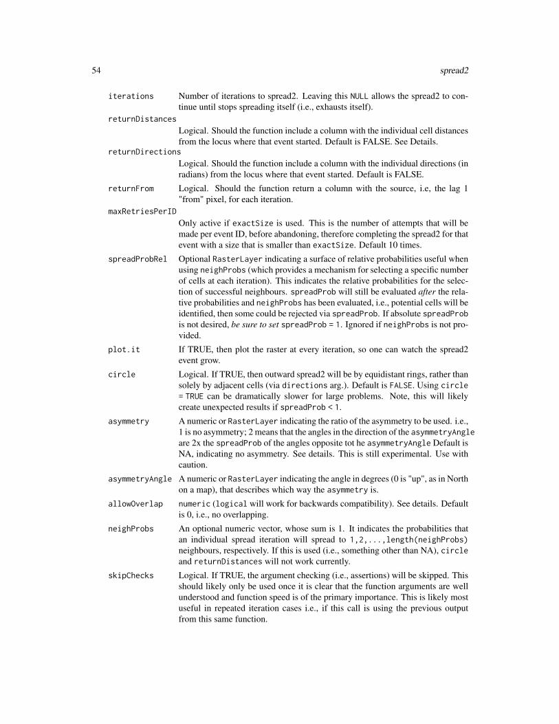
54 spread2

iterations Number of iterations to spread2. Leaving this NULL allows the spread2 to con-tinue until stops spreading itself (i.e., exhausts itself).

returnDistances


returnDirections

Logical. Should the function include a column with the individual directions (inradians) from the locus where that event started. Default is FALSE.

returnFrom Logical. Should the function return a column with the source, i.e, the lag 1"from" pixel, for each iteration.

maxRetriesPerID

Only active if exactSize is used. This is the number of attempts that will bemade per event ID, before abandoning, therefore completing the spread2 for thatevent with a size that is smaller than exactSize. Default 10 times.

spreadProbRel Optional RasterLayer indicating a surface of relative probabilities useful whenusing neighProbs (which provides a mechanism for selecting a specific numberof cells at each iteration). This indicates the relative probabilities for the selec-tion of successful neighbours. spreadProb will still be evaluated after the rela-tive probabilities and neighProbs has been evaluated, i.e., potential cells will beidentified, then some could be rejected via spreadProb. If absolute spreadProbis not desired, be sure to set spreadProb = 1. Ignored if neighProbs is not pro-vided.

plot.it If TRUE, then plot the raster at every iteration, so one can watch the spread2event grow.

circle Logical. If TRUE, then outward spread2 will be by equidistant rings, rather thansolely by adjacent cells (via directions arg.). Default is FALSE. Using circle= TRUE can be dramatically slower for large problems. Note, this will likelycreate unexpected results if spreadProb < 1.

asymmetry A numeric or RasterLayer indicating the ratio of the asymmetry to be used. i.e.,1 is no asymmetry; 2 means that the angles in the direction of the asymmetryAngleare 2x the spreadProb of the angles opposite tot he asymmetryAngle Default isNA, indicating no asymmetry. See details. This is still experimental. Use withcaution.

asymmetryAngle A numeric or RasterLayer indicating the angle in degrees (0 is "up", as in Northon a map), that describes which way the asymmetry is.

allowOverlap numeric (logical will work for backwards compatibility). See details. Defaultis 0, i.e., no overlapping.

neighProbs An optional numeric vector, whose sum is 1. It indicates the probabilities thatan individual spread iteration will spread to 1,2,...,length(neighProbs)neighbours, respectively. If this is used (i.e., something other than NA), circleand returnDistances will not work currently.

skipChecks Logical. If TRUE, the argument checking (i.e., assertions) will be skipped. Thisshould likely only be used once it is clear that the function arguments are wellunderstood and function speed is of the primary importance. This is likely mostuseful in repeated iteration cases i.e., if this call is using the previous outputfrom this same function.

spread2 55

Details

There are 2 main underlying algorithms for active cells to "spread" to nearby cells (adjacent cells):spreadProb and neighProb. Using spreadProb, every "active" pixel will assess all neighbours(either 4 or 8, depending on directions), and will "activate" whichever neighbours successfullypass independent calls to runif(1,0,1)<spreadProb. The algorithm will iterate again and again,each time starting from the newly "activated" cells. Several built-in decisions are as follows. 1.no active cell can active a cell that was already activated by the same event (i.e., "it won’t gobackwards"). 2. If allowOverlap is FALSE, then the previous rule will also apply, regardless ofwhich "event" caused the pixels to be previously active.

This function can be interrupted before all active cells are exhausted if the iterations value isreached before there are no more active cells to spread2 into. The interrupted output (a data.table)can be passed subsequently as an input to this same function (as start). This is intended to be usedfor situations where external events happen during a spread2 event, or where one or more argumentsto the spread2 function change before a spread2 event is completed. For example, if it is desiredthat the spreadProb change before a spread2 event is completed because, for example, a fire isspreading, and a new set of conditions arise due to a change in weather.

asymmetry here is slightly different than in the spread function, so that it can deal with a RasterLayerof asymmetryAngle. Here, the spreadProb values of a given set of neighbours around each activepixel are adjusted to create adjustedSpreadProb which is calculated maintain the following twoqualities:

mean(spreadProb) = mean(ajustedSpreadProb)

andmax(spreadProb)/min(spreadProb) = asymmetry

along the axis of asymmetryAngle. NOTE: this means that the 8 neighbours around an active cellmay not fulfill the preceeding equality if asymmetryAngle is not exactly one of the 8 angles of the8 neighbours. This means that

max(spreadProb)/min(spreadProb)

will generally be less than asymmetry, for the 8 neighbours. The exact adjustment to the spreadProbis calculated with:

angleQuality < −(cos(angles− rad(asymmetryAngle)) + 1)/2

which is multiplied to get an angle-adjusted spreadProb:

spreadProbAdj < −actualSpreadProb ∗ angleQuality

which is then rescaled:

adjustedSpreadProb = (spreadProbAdj −min(spreadProbAdj)) ∗ par2 + par1

, where par1 and par2 are parameters calculated internally to make the 2 conditions above true.

If exactSize or maxSize are used, then spreading will continue and stop before or at maxSize orat exactSize. If iterations is specified, then the function will end, and the returned data.tablewill still may (if maxSize) or will (if exactSize) have at least one active cell per event that didnot already achieve maxSize or exactSize. This will be very useful to build new, customizedhigher-level wrapper functions that iteratively call spread2.

56 spread2

Value

Either a data.table (asRaster=FALSE) or a RasterLayer (asRaster=TRUE, the default). Thedata.table will have one attribute named spreadState, which is a list containing a data.tableof current cluster-level information about the spread events. If asRaster=TRUE, then the data.table(with its spreadState attribute) will be attached to the Raster as an attribute named pixel as itprovides pixel-level information about the spread events.

The RasterLayer represents every cell in which a successful spread2 event occurred. For the caseof, say, a fire this would represent every cell that burned. If allowOverlap is TRUE, the return willalways be a data.table.

If asRaster is FALSE, then this function returns a data.table with 3 (or 4 if returnFrom is TRUE)columns:

initialPixels the initial cell number of that particular spread2 event.pixels The cell indices of cells that have been touched by the spread2 algorithm.state a logical indicating whether the cell is active (i.e., could still be a source for spreading) or not (no spreading will occur from these cells).from The pixel indices that were the immediately preceeding "source" for each pixels, i.e., the lag 1 pixels. Only returned if returnFrom is TRUE

The attribute saved with the name "spreadState" (e.g., attr(output,"spreadState")) includes adata.table with columns:

id An arbitrary code, from 1 to length(start) for each "event".initialPixels the initial cell number of that particular spread2 event.numRetries The number of re-starts the event did because it got stuck (normally only because exactSize was used and was not achieved.maxSize The number of pixels that were provided as inputs via maxSize or exactSize.size The current size, in pixels, of each event.

and several other objects that provide significant speed ups in iterative calls to spread2. If the userruns spread2 iteratively, there will likely be significant speed gains if the data.table passed in tostart should have the attribute attached, or re-attached if it was lost, e.g., via setattr(outInput,"spreadState",attr(out,"spreadState")),where out is the returned data.table from the previous call to spread2, and outInput is the mod-ified data.table. Currently, the modified data.table must have the same order as out.

Breaking out of spread2 events

There are 3 ways for the spread2 to "stop" spreading. Here, each "event" is defined as all cellsthat are spawned from each unique start location. The ways outlined below are all acting at alltimes, i.e., they are not mutually exclusive. Therefore, it is the user’s responsibility to make surethe different rules are interacting with each other correctly.

spreadProb Probabilistically, if spreadProb is low enough, active spreading events will stop. In practice, this number generally should be below 0.3 to actually see an event stopmaxSize This is the number of cells that are "successfully" turned on during a spreading event. spreadProb will still be active, so, it is possible that the end size of each event is smaller than maxSize, but they will not be greater than maxSizeexactSize This is the number of cells that are "successfully" turned on during a spreading event. This will override an event that stops probabilistically via spreadProb, but forcing its last set of active cells to try again to find neighbours. It will try maxRetriesPerID times per event, before giving up. During those maxRetriesPerID times, it will try to "jump" up to 4 cells outwards from each of the active cells, every 5 retries.iterations This is a hard cap on the number of internal iterations to complete before returning the current state of the system as a data.table.

spread2 57

Building custom spreading events

This function can be used iteratively, with relatively little overhead compared to using it non-iteratively. In general, this function can be called with arguments set as user needs, and with speci-fying iterations = 1 (say). This means that the function will spread outwards 1 iteration, then stop.The returned object will be a data.table or RasterLayer that can be passed immediately backas the start argument into a subsequent call to spread2. This means that every argument can beupdated at each iteration.

When using this function iteratively, there are several things to keep in mind. The output will likelybe sorted differently than the input (i.e., the order of start, if a vector, may not be the same orderas that returned). This means that when passing the same object back into the next iteration ofthe function call, maxSize or exactSize may not be in the same order. To get the same order,the easiest thing to do is sort the initial start objects by their pixel location, increasing. Then, ofcourse, sorting any vectorized arguments (e.g., maxSize) accordingly.

NOTE: the data.table or RasterLayer should not use be altered when passed back into spread2.

allowOverlap

If 1 (or TRUE), then individual events can overlap with one another, i.e., allow overlap betweenevents. If 2 (or NA), then each pixel is essentially independent, allowing overlap between and withinevents. This likely requires a user to intervene as it is possible to spread back onto itself. If 3(did not exist previously), individual events can overlap, and there can be overlap within an event,but only within an iteration, i.e., once an iteration is finished, and a pixel was activated, then thespreading will not return onto these pixels. If 0 (or FALSE), then once a pixel is activated, it cannotbe re-activated, within or between event. This allows events to not interfere with one another i.e.,they do not interact (this is slower than if allowOverlap = FALSE). Default is 0. In the case of 2 or3, this would be, perhaps, useful for dispersal of, say, insect swarms.

Note

exactSize may not be achieved if there aren’t enough cells in the map. Also, exactSize maynot be achieved because the active cells are "stuck", i.e., they have no unactivated cells to move to;or the spreadProb is low. In the latter two cases, the algorithm will retry again, but it will onlyre-try from the last iterations active cells. The algorithm will only retry 10 times before quitting.Currently, there will also be an attempt to "jump" up to four cells away from the active cells to tryto continue spreading.

A common way to use this function is to build wrappers around this, followed by iterative calls in awhile loop. See example.

Author(s)

Eliot McIntire and Steve Cumming

See Also

spread for a different implementation of the same algorithm. spread is less robust but it is oftenslightly faster.

58 spread2

Examples


data.table::setDTthreads(1)

a <- raster(extent(0, 10, 0, 10), res = 1)sams <- sort(sample(ncell(a), 3))

# Simple use -- similar to spread(...)out <- spread2(a, start = sams, 0.225)if (interactive()) {

clearPlot()Plot(out)

}

# Use maxSize -- this gives an upper limitmaxSizes <- sort(sample(1:10, size = length(sams)))out <- spread2(a, start = sams, 0.225, maxSize = maxSizes, asRaster = FALSE)# check TRUE using data.table .Nout[, .N, by = "initialPixels"]$N <= maxSizes

# Use exactSize -- gives an exact size, if there is enough space on the RasterexactSizes <- maxSizesout <- spread2(a, start = sams, spreadProb = 0.225,

exactSize = exactSizes, asRaster = FALSE)out[, .N, by = "initialPixels"]$N == maxSizes # should be TRUE TRUE TRUE

# Use exactSize -- but where it can't be achievedexactSizes <- sort(sample(100:110, size = length(sams)))out <- spread2(a, start = sams, 1, exactSize = exactSizes)

# Iterative calling -- create a function with a high escape probabilityspreadWithEscape <- function(ras, start, escapeProb, spreadProb) {

out <- spread2(ras, start = sams, spreadProb = escapeProb, asRaster = FALSE)while (any(out$state == "sourceActive")) {# pass in previous output as startout <- spread2(ras, start = out, spreadProb = spreadProb,

asRaster = FALSE, skipChecks = TRUE) # skipChecks for speed}out

}

set.seed(421)out1 <- spreadWithEscape(a, sams, escapeProb = 0.25, spreadProb = 0.225)set.seed(421)out2 <- spread2(a, sams, 0.225, asRaster = FALSE)# The one with high escape probability is larger (most of the time)NROW(out1) > NROW(out2)

## Use neighProbs, with a spreadProb that is a RasterLayer

spread2 59

# Create a raster of different values, which will be the relative probabilities# i.e., they are rescaled to relative probabilities within the 8 neighbour choices.# The neighProbs below means 70% of the time, 1 neighbour will be chosen,# 30% of the time 2 neighbours.# The cells with spreadProb of 5 are 5 times more likely than cells with 1 to be chosen,# when they are both within the 8 neighbourssp <- raster(extent(0, 3, 0, 3), res = 1, vals = 1:9) #small raster, simple values# Check neighProbs workedout <- list()

# enough replicates to see stabilized probabilitiesfor (i in 1:100) {

out[[i]] <- spread2(sp, spreadProbRel = sp, spreadProb = 1,start = 5, iterations = 1,neighProbs = c(1), asRaster = FALSE)

}out <- data.table::rbindlist(out)[pixels != 5] # remove starting celltable(sp[out$pixels])# should be non-significant -- note no 5 because that was the starting cell# This tests whether the null model is true ... there should be proportions# equivalent to 1:2:3:4:6:7:8:9 ... i.e,. cell 9 should have 9x as many events# spread to it as cell 1. This comes from sp object above which is providing# the relative spread probabilitieskeep <- c(1:4, 6:9)chisq.test(keep, unname(tabulate(sp[out$pixels], 9)[keep]), simulate.p.value = TRUE)

## Example showing asymmetrysams <- ncell(a) / 4 - ncol(a) / 4 * 3circs <- spread2(a, spreadProb = 0.213, start = sams,

asymmetry = 2, asymmetryAngle = 135,asRaster = TRUE)

## ADVANCED: Estimate spreadProb when using asymmetry, such that the expected## event size is the same as without using asymmetry## Not run:

if (interactive()) {ras <- raster(a)ras[] <- 1

n <- 100sizes <- integer(n)for (i in 1:n) {

circs <- spread2(ras, spreadProb = 0.225,start = round(ncell(ras) / 4 - ncol(ras) / 4 * 3),asRaster = FALSE)

sizes[i] <- circs[, .N]}goalSize <- mean(sizes)

library(parallel)library(DEoptim)

cl <- makeCluster(pmin(10, detectCores() - 2)) # need 10 cores for 10 populations in DEoptimparallel::clusterEvalQ(cl, {

60 spread3

library(SpaDES.tools)library(raster)library(fpCompare)

})

objFn <- function(sp, n = 20, ras, goalSize) {sizes <- integer(n)for (i in 1:n) {circs <- spread2(ras, spreadProb = sp, start = ncell(ras) / 4 - ncol(ras) / 4 * 3,

asymmetry = 2, asymmetryAngle = 135,asRaster = FALSE)

sizes[i] <- circs[, .N]}abs(mean(sizes) - goalSize)

}aa <- DEoptim(objFn, lower = 0.2, upper = 0.23,

control = DEoptim.control(cluster = cl, NP = 10, VTR = 0.02,initialpop = as.matrix(rnorm(10, 0.213, 0.001))),

ras = a, goalSize = goalSize)

# The value of spreadProb that will give the same expected event sizes to spreadProb = 0.225 is:sp <- aa$optim$bestmemcircs <- spread2(ras, spreadProb = sp, start = ncell(ras) / 4 - ncol(ras) / 4 * 3,

asymmetry = 2, asymmetryAngle = 135, asRaster = FALSE)

stopCluster(cl)}

## End(Not run)

spread3 An alternative spread function, conceived for insects

Description

This is built with spread2 and is still experimental. This one differs from other attempts in thatit treats the advection and dispersal as mathematical vectors that are added together. They are"rounded" to pixel centres.

Usage

spread3(start,rasQuality,rasAbundance,advectionDir,advectionMag,meanDist,dispersalKernel = "exponential",

spread3 61

sdDist = 1,plot.it = 2,minNumAgents = 50,verbose = getOption("LandR.verbose", 0),saveStack = NULL,skipChecks = FALSE

)

Arguments

start Raster indices from which to initiate dispersal

rasQuality A raster with habitat quality. Currently, must be scaled from 0 to 1, i.e., a prob-ability of "settling"

rasAbundance A raster where each pixel represents the number of "agents" or pseudo-agentscontained. This number of agents, will be spread horizontally, and distributedfrom each pixel that contains a non-zero non NA value.

advectionDir A single number or RasterLayer in degrees from North = 0 (though it willuse radians if all values are abs(advectionDir) > 2 * pi). This indicates thedirection of advective forcing (i.e., wind).

advectionMag A single number or RasterLayer in distance units of the rasQuality, e.g.,meters, indicating the relative forcing that will occur. It is imposed on the to-tal event, i.e., if the meanDist is 10000, and advectionMag is 5000, then theexpected distance (i.e., 63% of agents) will have settled by 15000 map units.

meanDist A single number indicating the mean distance parameter in map units (not pix-els), for a negative exponential distribution dispersal kernel (e.g., dexp). Thiswill mean that 63 settled at this meanDist (still experimental)

dispersalKernel

One of either "exponential" or "weibull". If

sdDist A single number indicating the sd parameter of a two-parameter dispersalKernel.Defaults to 1, which is the same as the exponential distribution.

plot.it Numeric. With increasing numbers above 0, there will be plots produced duringiterations. Currently, only 0, 1, or 2+ are distinct.

minNumAgents Single numeric indicating the minimum number of agents to consider all dis-persing finished. Default is 50

verbose Numeric. With increasing numbers above 0, there will be more messages pro-duced. Currently, only 0, 1, or 2+ are distinct.

saveStack If provided as a character string, it will save each iteration as part of a rasterStackto disk upon exit.

skipChecks Logical. If TRUE, assertions will be skipped (faster, but could miss problems)

Value

A data.table with all information used during the spreading

62 spread3

Examples

## these tests are fairly heavy, so don't run during automated testsif (interactive() && require("RandomFields")) {

########################################################## Simple case, no variation in rasQuality, numeric advectionDir and advectionMag#########################################################library(raster)library(quickPlot)maxDim <- 10000ras <- raster::raster(extent(c(0, maxDim, 0, maxDim)), res = 100, vals = 0)rasQuality <- raster(ras)rasQuality[] <- 1rasAbundance <- raster(rasQuality)rasAbundance[] <- 0# startPixel <- middlePixel(rasAbundance)startPixel <- sample(seq(ncell(rasAbundance)), 30)rasAbundance[startPixel] <- 1000advectionDir <- 70advectionMag <- 4 * res(rasAbundance)[1]meanDist <- 2600

if (interactive()) {# Test the dispersal kernel -- create a functionplotDispersalKernel <- function(out, meanAdvectionMag) {

out[, disGroup := round(distance / 100) * 100]freqs <- out[, .N, by = "disGroup"]freqs[, `:=`(cumSum = cumsum(N), N = N)]Plot(freqs$disGroup, freqs$cumSum, addTo = "CumulativeNumberSettled",

title = "Cumulative Number Settled") # can plot the distance X numberabline(v = meanAdvectionMag + meanDist)newTitle <- "Number Settled By Distance"Plot(freqs$disGroup, freqs$N, addTo = gsub(" ", "", newTitle),

title = newTitle) # can plot the distance X numberabline(v = meanAdvectionMag + meanDist)# should be 0.63:freqs[disGroup == meanAdvectionMag + meanDist, cumSum] / tail(freqs,1)[, cumSum]mtext(side = 3, paste("Average habitat quality: ",

round(mean(rasQuality[], na.rm = TRUE), 2)),outer = TRUE, line = -2, cex = 2)

}dev() # don't use Rstudio windows, which is very slowclearPlot()out <- spread3(rasAbundance = rasAbundance,

rasQuality = rasQuality,advectionDir = advectionDir,advectionMag = advectionMag,meanDist = meanDist, verbose = 2,plot.it = 2)

plotDispersalKernel(out, advectionMag)}

spread3 63

############################################################ The case of variable quality raster#########################################################if (require(sf) && require(fasterize)) {

library(SpaDES.tools) # for gaussMapa <- randomStudyArea(size = 1e9)ras <- raster(extent(a), res = 100)mask <- fasterize(st_as_sf(a), ras) # faster than raster::rasterizerasQuality <- gaussMap(ras)crs(rasQuality) <- crs(a)rasQuality[is.na(mask)] <- NA# rescale so min is 0.75 and max is 1rasQuality[] <- rasQuality[] / (maxValue(rasQuality) * 4 ) + 1/4rasAbundance <- raster(rasQuality)rasAbundance[] <- 0startPixel <- sample(seq(ncell(rasAbundance)), 300)rasAbundance[startPixel] <- 1000advectionDir <- 75advectionMag <- 4 * res(rasAbundance)[1]meanDist <- 2600clearPlot()out <- spread3(rasAbundance = rasAbundance,

rasQuality = rasQuality,advectionDir = advectionDir,advectionMag = advectionMag,meanDist = meanDist, verbose = 2,plot.it = 1)

if (interactive()) {plotDispersalKernel(out, advectionMag)

}}

################################################################################## The case of variable quality raster, raster for advectionDir & advectionMag###############################################################################library(raster)library(quickPlot)library(SpaDES.tools)maxDim <- 10000ras <- raster(extent(c(0, maxDim, 0, maxDim)), res = 100, vals = 0)rasQuality <- raster(ras)rasQuality[] <- 1rasAbundance <- raster(rasQuality)rasAbundance[] <- NA# startPixel <- middlePixel(rasAbundance)startPixel <- sample(seq(ncell(rasAbundance)), 25)rasAbundance[startPixel] <- 1000

# raster for advectionDiradvectionDir <- gaussMap(ras)crs(advectionDir) <- crs(rasQuality)# rescale so min is 0.75 and max is 1advectionDir[] <- advectionDir[] / (maxValue(advectionDir)) * 180

64 testEquivalentMetadata

# raster for advectionMagadvectionMag <- gaussMap(ras)crs(advectionMag) <- crs(rasQuality)# rescale so min is 0.75 and max is 1advectionMag[] <- advectionMag[] / (maxValue(advectionMag)) * 600

out <- spread3(rasAbundance = rasAbundance,rasQuality = rasQuality,advectionDir = advectionDir,advectionMag = advectionMag,meanDist = meanDist, verbose = 2,plot.it = 1)

if (interactive()) {dev() # don't use Rstudio windows, which is very slowclearPlot()Plot(advectionDir, title = "Wind direction", cols = "Reds")Plot(advectionMag, title = "Wind speed", cols = "Blues")plotDispersalKernel(out, mean(advectionMag[]))Plot(rasAbundance, addTo = "rasAbundance", cols = "black", title = "")

}

########################################## save iterations to a stack to make animated GIF########################################tmpStack <- raster::rasterTmpFile("stackToAnimate")out <- spread3(rasAbundance = rasAbundance,

rasQuality = rasQuality,advectionDir = advectionDir,advectionMag = advectionMag,meanDist = 2600, verbose = 2,plot.it = 0, saveStack = tmpStack)

## This animates the series of images into an animated GIFif (require(animation, quietly = TRUE)) {

out2 <- raster::stack(tmpStack)gifName <- file.path(tempdir(), "animation.gif")saveGIF(interval = 0.1, movie.name = gifName, expr = {

for (i in seq(numLayers(out2))) plot(out2[[i]])})

}}

testEquivalentMetadata

Test that metadata of 2 or more objects is the same

transitions 65

Description

Currently, only Raster class has a useful method. Defaults to all(sapply(list(...)[-1],function(x)identical(list(...)[1],x)))

Usage

testEquivalentMetadata(...)

Arguments

... 2 or more of the same type of object to test for equivalent metadata

transitions SELES - Transitioning to next time step

Description

Describes the probability of an agent successfully persisting until next time step. THIS IS NOTYET FULLY IMPLEMENTED.



Usage

transitions(p, agent)

Arguments

p realized probability of persisting (i.e., either 0 or 1).

agent SpatialPoints* object.

Value

Returns new SpatialPoints* object with potentially fewer agents.

Author(s)

Eliot McIntire


66 wrap

wrap Wrap coordinates or pixels in a torus-like fashion

Description

Generally useful for model development purposes.

Usage

wrap(X, bounds, withHeading)

## S4 method for signature 'matrix,Extent,missing'wrap(X, bounds)

## S4 method for signature 'SpatialPoints,ANY,missing'wrap(X, bounds)

## S4 method for signature 'matrix,Raster,missing'wrap(X, bounds)

## S4 method for signature 'matrix,Raster,missing'wrap(X, bounds)

## S4 method for signature 'matrix,matrix,missing'wrap(X, bounds)

## S4 method for signature 'SpatialPointsDataFrame,Extent,logical'wrap(X, bounds, withHeading)

## S4 method for signature 'SpatialPointsDataFrame,Raster,logical'wrap(X, bounds, withHeading)

## S4 method for signature 'SpatialPointsDataFrame,matrix,logical'wrap(X, bounds, withHeading)

Arguments

X A SpatialPoints* object, or matrix of coordinates.

bounds Either a Raster*, Extent, or bbox object defining bounds to wrap around.

withHeading logical. If TRUE, the previous points must be wrapped also so that the subsequentheading calculation will work. Default FALSE. See details.

Details

If withHeading used, then X must be a SpatialPointsDataFrame that contains two columns, x1and y1, with the immediately previous agent locations.

wrap 67

Value

Object of the same class as X, but with coordinates updated to reflect the wrapping.

Author(s)

Eliot McIntire

Examples


xrange <- yrange <- c(-50, 50)hab <- raster(extent(c(xrange, yrange)))hab[] <- 0

# initialize agentsN <- 10

# previous pointsx1 <- rep(0, N)y1 <- rep(0, N)# initial pointsstarts <- cbind(x = stats::runif(N, xrange[1], xrange[2]),

y = stats::runif(N, yrange[1], yrange[2]))

# create the agent objectagent <- SpatialPointsDataFrame(coords = starts, data = data.frame(x1, y1))

ln <- rlnorm(N, 1, 0.02) # log normal step lengthsd <- 30 # could be specified globally in params

if (interactive()) {clearPlot()Plot(hab, zero.color = "white", axes = "L")

}for (i in 1:10) {

agent <- crw(agent = agent, extent = extent(hab), stepLength = ln,stddev = sd, lonlat = FALSE, torus = TRUE)

if (interactive()) Plot(agent, addTo = "hab", axes = TRUE)}

Index

.cirSpecialQuick (cirSpecialQuick), 12

.pointDistance, 5

adj, 3, 6adjacent, 3, 8agentLocation, 4, 8

beginCluster, 14, 25buffer, 46

cellFromXY, 35, 43, 53cir, 3, 9, 15, 36, 47cirSpecialQuick, 12crw, 3crw (move), 27crw,SpatialPoints-method (move), 27crw,SpatialPointsDataFrame-method

(move), 27

directionFromEachPoint, 3distanceFromEachPoint, 3, 10, 13distanceFromPoints, 13, 15, 47do.call, 25duplicatedInt, 16dwrpnorm, 17dwrpnorm2, 17

endCluster, 25equalExtent, 4extent, 19

fastCrop, 18focal, 46

gaussMap, 4, 18, 32

heading, 3, 20heading,matrix,matrix-method (heading),

20heading,matrix,SpatialPoints-method

(heading), 20

heading,SpatialPoints,matrix-method(heading), 20

heading,SpatialPoints,SpatialPoints-method(heading), 20

initiateAgents, 4, 21initiateAgents,Raster,missing,missing,ANY,missing-method

(initiateAgents), 21initiateAgents,Raster,missing,missing,ANY,numeric-method

(initiateAgents), 21initiateAgents,Raster,missing,Raster,ANY,missing-method

(initiateAgents), 21initiateAgents,Raster,numeric,missing,ANY,missing-method

(initiateAgents), 21initiateAgents,Raster,numeric,Raster,ANY,missing-method

(initiateAgents), 21inRange, 23

makeLines, 3merge, 25mergeRaster, 24mergeRaster,list-method (mergeRaster),

24middlePixel, 27mosaic, 25move, 3, 27

numAgents, 4, 22, 29

options, 4

patchSize, 29pointDistance, 28pointDistance (.pointDistance), 5probInit, 4, 22, 30

randomPolygon (randomPolygons), 31randomPolygons, 4, 31, 32randomStudyArea, 32raster, 32, 34rasterizeReduced, 4, 33

68

INDEX 69

rings, 3, 10, 15, 34, 47rings,RasterLayer-method (rings), 34runifC, 37

SpaDES.tools (SpaDES.tools-package), 3SpaDES.tools-package, 3SpatialPoints*, 3specificNumPerPatch, 3, 37splitRaster (mergeRaster), 24splitRaster,RasterLayer-method

(mergeRaster), 24spokes, 3, 38spokes,RasterLayer,SpatialPoints,missing-method

(spokes), 38spread, 3, 31, 32, 34, 41, 57spread,RasterLayer-method (spread), 41spread2, 41, 47, 52, 60spread3, 60

testEquivalentMetadata, 64transitions, 4, 65

wrap, 3, 66wrap,matrix,Extent,missing-method

(wrap), 66wrap,matrix,matrix,missing-method

(wrap), 66wrap,matrix,Raster,missing-method

(wrap), 66wrap,SpatialPoints,ANY,missing-method

(wrap), 66wrap,SpatialPointsDataFrame,Extent,logical-method

(wrap), 66wrap,SpatialPointsDataFrame,matrix,logical-method

(wrap), 66wrap,SpatialPointsDataFrame,Raster,logical-method

(wrap), 66writeRaster, 18

Package 'SpaDES.tools'

Documents

Transcript of Package 'SpaDES.tools'