An Empirical Bayes Approach to Shrinkage Estimation ... - arXiv

An Empirical Bayes Approach to ShrinkageEstimation on the Manifold of Symmetric

Positive-Definite Matrices∗†

Chun-Hao Yang1, Hani Doss1 and Baba C. Vemuri21Department of Statistics

2Department of Computer Information Science & EngineeringUniversity of Florida

October 28, 2020

Abstract

The James-Stein estimator is an estimator of the multivariate normal mean anddominates the maximum likelihood estimator (MLE) under squared error loss. Theoriginal work inspired great interest in developing shrinkage estimators for a varietyof problems. Nonetheless, research on shrinkage estimation for manifold-valued datais scarce. In this paper, we propose shrinkage estimators for the parameters of theLog-Normal distribution defined on the manifold of N ×N symmetric positive-definitematrices. For this manifold, we choose the Log-Euclidean metric as its Riemannianmetric since it is easy to compute and is widely used in applications. By using theLog-Euclidean distance in the loss function, we derive a shrinkage estimator in an ana-lytic form and show that it is asymptotically optimal within a large class of estimatorsincluding the MLE, which is the sample Frechet mean of the data. We demonstratethe performance of the proposed shrinkage estimator via several simulated data exper-iments. Furthermore, we apply the shrinkage estimator to perform statistical inferencein diffusion magnetic resonance imaging problems.

Keywords: Stein’s unbiased risk estimate, Frechet mean, Tweedie’s estimator

∗This research was in part funded by the NSF grants IIS-1525431 and IIS-1724174 to Vemuri.†This manuscript has been submitted to a journal.

1

arX

iv:2

007.

0215

3v3

[m

ath.

ST]

27

Oct

202

0

1 Introduction

Symmetric positive-definite (SPD) matrices are common in applications of science and en-

gineering. In computer vision problems, they are encountered in the form of covariance

matrices, e.g. region covariance descriptor (Tuzel et al. 2006), and in diffusion magnetic

resonance imaging, SPD matrices manifest themselves as diffusion tensors which are used

to model the diffusion of water molecules (Basser et al. 1994) and as Cauchy deformation

tensors in morphometry to model the deformations (see Frackowiak et al. (2004, Ch. 36)).

Many other applications can be found in Cherian & Sra (2016). In such applications, the

statistical analysis of data must perform geometry-aware computations, i.e. employ methods

that take into account the nonlinear geometry of the data space. In most data analysis

applications, it is useful to describe the entire dataset with a few summary statistics. For

data residing in Euclidean space, this may simply be the sample mean, and for data resid-

ing in non-Euclidean spaces, e.g. Riemannian manifolds, the corresponding statistic is the

sample Frechet mean (FM) (Frechet 1948). The sample FM also plays an important role in

different statistical inference methods, e.g. principal geodesic analysis (Fletcher et al. 2003),

clustering algorithms, etc. If M is a metric space with metric d, and x1, . . . , xn ∈ M , the

sample FM is defined by x = arg minm∑n

i=1 d2(xi,m). For Riemannian manifolds, the dis-

tance is usually chosen to be the intrinsic distance induced by the Riemannian metric. Then,

the above optimization problem can be solved by Riemannian gradient descent algorithms

(Pennec 2006, Groisser 2004, Afsari 2011, Moakher 2005). However, Riemannian gradient

descent algorithms are usually computationally expensive, and efficient recursive algorithms

for computing the sample FM have been presented in the literature for various Riemannian

manifolds by Sturm (2003), Ho et al. (2013), Salehian et al. (2015), Chakraborty & Vemuri

(2015), Lim & Palfia (2014) and Chakraborty & Vemuri (2019).

In Rp with the Euclidean metric, the sample FM is just the ordinary sample mean.

Consider a set of normally distributed random variables X1, . . . , Xn. The sample mean

X = n−1∑n

i=1Xi is the maximum likelihood estimator (MLE) for the mean of the underlying

normal distribution, and the James-Stein (shrinkage) estimator (James & Stein 1962) was

shown to be better (under squared error loss) than the MLE when p > 2 and the covariance

2

matrix of the underlying normal distribution is assumed to be known. Inspired by this result,

the goal of this paper is to develop shrinkage estimators for data residing in PN , the space

of N ×N SPD matrices.

For the model Xiind∼ N(µi, σ

2) where p > 2 and σ2 is known, the MLE of µ = [µ1, . . . , µp]T

is µMLE = [X1, . . . , Xp]T and it is natural to ask whether the MLE is admissible. Stein (1956)

gave a negative answer to this question and provided a class of estimators for µ that dominate

the MLE. Subsequently, James & Stein (1962) proposed the estimator(1− (p− 2)σ2

‖X‖2

)X (1)

where X = [X1, . . . , Xp]T , which was later referred to as the James-Stein (shrinkage) esti-

mator.

Ever since the work reported in James & Stein (1962), generalizations or variants of

this shrinkage estimator have been developed in a variety of settings. A few directions

for generalization are as follows. First, instead of estimating the means of many normal

distributions, carry out the simultaneous estimation of parameters (e.g. the mean or the scale

parameter) of other distributions, e.g. Poisson, Gamma, etc.; see Johnson (1971), Fienberg

& Holland (1973), Clevenson & Zidek (1975), Tsui (1981), Tsui & Press (1982), Brandwein

& Strawderman (1990) and Brandwein & Strawderman (1991). More recent works include

Xie et al. (2012), Xie et al. (2016), Jing et al. (2016), Kong et al. (2017), Muandet et al.

(2016), Hansen (2016), and Feldman et al. (2014). Second, since the MLE of the mean of a

normal distribution is also the best translation-equivariant estimator but is inadmissible, an

interesting question to ask is, when is the best translation-equivariant estimator admissible?

This problem was studied extensively in Stein (1959) and Brown (1966).

Besides estimation of the mean of different distributions, estimation of the covariance ma-

trix (or the precision matrix) of a multivariate normal distribution is an important problem in

statistics, finance, engineering and many other fields. The usual estimator, namely the sam-

ple covariance matrix, performs poorly in high-dimensional problems and many researchers

have endeavored to improve covariance estimation by applying the concept of shrinkage in

this context (Stein 1975, Haff 1991, Daniels & Kass 2001, Ledoit & Wolf 2003, Daniels &

Kass 2001, Ledoit & Wolf 2012, Donoho et al. 2018). Note that there is a vast literature

3

on covariance estimation and we only cited a few references here. For a thorough literature

review, we refer the interested reader to Donoho et al. (2018).

In order to understand shrinkage estimation fully, one must understand why the process

of shrinkage improves estimation. In this context, Efron and Morris presented a series

of works to provide an empirical Bayes interpretation by modifying the original James-

Stein estimator to suit different problems (Efron & Morris 1971, 1972b,a, 1973b,a). The

empirical Bayes approach to designing a shrinkage estimator can be described as follows.

First, reformulate the model as a Bayesian model, i.e. place a prior on the parameters.

Then, the hyper-parameters of the prior are estimated from the data. Efron & Morris

(1973b) presented several examples of different shrinkage estimators developed within this

empirical Bayes framework. An alternative, non-Bayesian, geometric interpretation to Stein

shrinkage estimation was presented by Brown & Zhao (2012).

In all the works cited above, the domain of the data has invariably been a vector space

and, as mentioned earlier, many applications naturally encounter data residing in non-

Euclidean spaces. Hence, generalizing shrinkage estimation to non-Euclidean spaces is a

worthwhile pursuit. In this paper, we focus on shrinkage estimation for the Riemannian

manifold PN . We assume that the observed SPD matrices are drawn from a Log-Normal

distribution defined on PN (Schwartzman 2016) and we are interested in estimating the

mean and the covariance matrix of this distribution. We derive shrinkage estimators for the

parameters of the Log-Normal distribution using an empirical Bayes framework (Xie et al.

2012), which is described in detail subsequently, and show that the proposed estimator is

asymptotically optimal within a class of estimators including the MLE. We describe sim-

ulated data experiments which demonstrate that the proposed shrinkage estimator of the

mean of the Log-Normal distribution is better (in terms of risk) than the sample FM, which

is the MLE, and the shrinkage estimator proposed by Yang & Vemuri (2019). Further, we

also apply the shrinkage estimator to find group differences between patients with Parkin-

son’s disease and controls (normal subjects) from their respective brain scans acquired using

diffusion magnetic resonance images (dMRIs).

The rest of this paper is organized as follows. In section 2, we present relevant material on

the Riemannian geometry of PN and shrinkage estimation. The main theoretical results are

4

stated in section 3 with the proofs of the theorems relegated to the supplement. In section 4,

we demonstrate how the proposed shrinkage estimators perform via several synthetic data

examples and present applications to (real data) diffusion tensor imaging (DTI), a clinically

popular version of dMRI. Specifically, we apply the proposed shrinkage estimator to the

estimation of the brain atlases (templates) of patients with Parkinson’s disease and a control

group and identify the regions of the brain where the two groups differ significantly. Finally,

in section 5 we discuss our contributions and present some future research directions.

2 Preliminaries

In this section, we briefly review the commonly used Log-Euclidean metric for PN (Arsigny

et al. 2007) and the concept of Stein’s unbiased risk estimate, which will form the framework

for deriving the shrinkage estimators.

2.1 Riemannian Geometry of PN

In this work, we endow the manifold PN with the Log-Euclidean metric proposed by Arsigny

et al. (2007). We note that there is another commonly used Riemannian metric on PN ,

called the affine-invariant metric (see Terras (2016, Ch. 1) for its introduction and Lenglet,

Rousson, Deriche & Faugeras (2006) and Moakher (2005) for its applications). The affine-

invariant metric is computationally more expensive and in some applications it provides

results that are indistinguishable from those obtained under the Log-Euclidean metric as

demonstrated in Arsigny et al. (2007) and Schwartzman (2016). Based on this reasoning, we

choose to work with the Log-Euclidean metric. For other metrics on PN used in a variety of

applications, we refer the reader to a recent survey (Feragen & Fuster 2017).

The Log-Euclidean metric is a bi-invariant Riemannian metric on the abelian Lie group

(PN ,�) where X � Y = exp(logX + log Y ). The intrinsic distance dLE : PN × PN → R

induced by the Log-Euclidean metric has a very simple form, namely

dLE(X, Y ) = ‖logX − log Y ‖

5

where ‖ · ‖ is the Frobenius norm. Consider the map vec : Sym(N)→ RN(N+1)

2 defined by

vec(Y ) =[y11, . . . , ynn,

√2(yij)i<j

]T(Schwartzman 2016). This map is actually an isomorphism between Sym(N) and R

N(N+1)2 .

To make the notation more concise, for X ∈ PN , we denote X = vec(logX) ∈ RN(N+1)

2 .

From the definition of vec, we see that dLE(X, Y ) = ‖X − Y ‖.

Given X1, . . . , Xn ∈ PN , we denote the sample FM with respect to the two intrinsic

distances given above by

X = arg minM∈PN

n−1

n∑i=1

d2LE(Xi,M) = exp

(n−1

n∑i=1

logXi

). (2)

2.2 The Log-Normal Distribution on PN

In this work, we assume that the observed SPD matrices follow the Log-Normal distribution

introduced by Schwartzman (2006), which can be viewed as a generalization of the Log-

Normal distribution on R+ to PN . The definition of the Log-Normal distribution is stated

as follows.

Definition 1 Let X be a PN -valued random variable. We say X follows a Log-Normal

distribution with mean M ∈ PN and covariance matrix Σ ∈ PN(N+1)/2, or X ∼ LN(M,Σ), if

X ∼ N(M,Σ).

From the definition, it is easy to see that E logX = logM and E‖logX − logM‖2 =

E‖X − M‖2 = tr(Σ). Some important results regarding this distribution were obtained

in Schwartzman (2016). The following proposition for the MLEs of the parameters will be

useful subsequently in this work.

Proposition 1 Let X1, . . . , Xniid∼ LN(M,Σ). Then, the MLEs of M and Σ are MMLE = X

and ΣMLE = n−1∑n

i=1

(Xi −

˜MMLE

)(Xi −

˜MMLE

)T. The MLE of M is the sample FM

under the Log-Euclidean metric.

2.3 Bayesian Formulation of Shrinkage Estimation in Rp

As discussed earlier, the James-Stein estimator originated from the problem of simultane-

ous estimation of multiple means of (univariate) normal distributions. The derivation relied

6

heavily on the properties of the univariate normal distribution. Later on, Efron & Mor-

ris (1973b) gave an empirical Bayes interpretation for the James-Stein estimator, which is

presented by considering the hierarchical model

Xi|θiind∼ N(θi, A), i = 1, . . . , p,

θiiid∼ N(µ, λ),

where A is known and µ and λ are unknown. The posterior mean for θi is

θλ,µi =λ

λ+ AXi +

A

λ+ Aµ. (3)

The parametric empirical Bayes method for estimating the θi’s consists of first estimating

the prior parameters λ and µ and then substituting them into (3). The prior parameters λ

and µ can be estimated by the MLE. For the special case of µ = 0, this method produces

an estimator similar to the James-Stein estimator (1). Although this estimator is derived

in an (empirical) Bayesian framework, it is of interest to determine whether it has good

frequentist properties. For example, if we specify a loss function L and consider the induced

risk function R, one would like to determine whether the estimator has uniformly smallest

risk within a reasonable class of estimators. In (3), the optimal choice of λ and µ is

(λopt, µopt

)= arg min

λ,µR(θλ,µ,θ),

where θ = [θ1, . . . , θp]T , θ

λ,µ= [θλ,µ1 , . . . , θλ,µp ]T , and λopt and µopt depend on θ, which is

unknown. Instead of minimizing the risk function directly, we will minimize Stein’s unbiased

risk estimate (SURE) (Stein 1981), denoted by SURE(λ, µ), which satisfiesEθ [SURE(λ, µ)] =

R(θλ,µ,θ). Thus, we will use

(λSURE, µSURE

)= arg min

λ,µSURE(λ, µ).

The challenging part of this endeavor is to derive SURE, which depends heavily on the risk

function and the underlying distribution of the data. This approach has been used to derive

estimators for many models. For example, Xie et al. (2012) derived the (asymptotically)

optimal shrinkage estimator for a heteroscedastic hierarchical model, and their result is

further generalized in Jing et al. (2016) and Kong et al. (2017).

7

3 An Empirical Bayes Shrinkage Estimator for Log-

Normal Distributions

In this section, we consider the model

Xijind∼ LN(Mi,Σi), i = 1, . . . , p, j = 1, . . . , n,

and develop shrinkage estimators for the mean M = [M1, . . . ,Mp] and the covariance matrix

Σ = [Σ1, . . . ,Σp]. These Xij’s are PN -valued random matrices. For completeness, we first

briefly review the shrinkage estimator proposed by Yang & Vemuri (2019) for M assuming

Σi = AiI, where the Ai’s are known positive numbers and I is the identity matrix. The

assumption on Σ is useful when n is small since for small sample sizes the MLE for Σ is

very unstable. Next, we present estimators for both M and Σ. Besides presenting these

estimators, we establish asymptotic optimality results for the proposed estimators. To be

more precise, we show that the proposed estimators are asymptotically optimal within a

large class of estimators containing the MLE.

Another related interesting problem often encountered in practice involves group testing

and estimating the “difference” between the two given groups. Consider the model

Xijind∼ LN(M

(1)i ,Σ

(1)i ), i = 1, . . . , p, j = 1, . . . , nx,

Yijind∼ LN(M

(2)i ,Σ

(2)i ), i = 1, . . . , p, j = 1, . . . , ny,

where the Xij’s and Yij’s are independent. We want to estimate the differences between

M(1)i and M

(2)i for i = 1, . . . , p and select the i’s for which the differences are large. However,

the selected estimates tend to overestimate the corresponding true differences. The bias

introduced by the selection process is termed by selection bias (Dawid 1994). The selection

bias originates from the fact that there are two possible reasons for the selected differences

to be large: (i) the true differences are large and (ii) the random errors contained in the

estimates are large. Tweedie’s formula (Efron 2011), which we discuss and briefly review

in section 3.3, deals with precisely this selection bias, in the context of the normal means

problem. In this work, we apply an analogue of Tweedie’s formula designed for the context

of SPD matrices.

8

3.1 An Estimator of M When Σ is Known

For completeness, we briefly review the work of Yang & Vemuri (2019) where the authors

presented the estimator for M assuming that Σi = AiI where the Ai’s are known positive

numbers. Under this assumption, they considered the class of estimators given by

Mλ,µi = exp

(nλ

nλ+ Ailog Xi +

Ainλ+ Ai

log µ

), (4)

where µ ∈ PN , λ > 0, and Xi is the sample FM of Xi1, . . . , Xin. Using the Log-Euclidean

distance as the loss function L(M ,M) = p−1∑p

i=1 d2LE(Mi,Mi), they showed that the SURE

for the corresponding risk function R(M ,M ) = EL(M ,M ) is given by

SURE(λ, µ) =1

p

p∑i=1

Ai(nλ+ Ai)2

(Ai‖log Xi − log µ‖2 +

q(n2λ2 − A2i )

n

).

Hence, λ and µ can be estimated by(λSURE, µSURE

)= arg min

λ,µSURE(λ, µ). (5)

Their shrinkage estimator for Mi is given by

MSUREi = exp

(nλSURE

nλSURE + Ailog Xi +

Ai

nλSURE + Ailog µSURE

). (6)

They also presented the following two theorems showing the asymptotic optimality of the

shrinkage estimator.

Theorem 1 Assume the following conditions:

(i) lim supp→∞ p−1∑p

i=1A2i <∞,

(ii) lim supp→∞ p−1∑p

i=1Ai‖logMi‖2 <∞,

(iii) lim supp→∞ p−1∑p

i=1 ‖logMi‖2+δ <∞ for some δ > 0.

Then,

supλ>0,‖logµ‖<maxi ‖log Xi‖

|SURE(λ, µ)− L(Mλ,µ,M)| prob−→ 0 as p→∞.

Theorem 2 If assumptions (i), (ii) and (iii) in Theorem 1 hold, then

limp→∞

[R(MSURE

,M )−R(Mλ,µ,M )] ≤ 0.

9

3.2 Estimators for M and Σ

In Yang & Vemuri (2019), the covariance matrices of the underlying distributions were

assumed to be known to simplify the derivation. In real applications however, the covariance

matrices are rarely known, and in practice they must be estimated. In this paper, we consider

the general case of unknown covariance matrices which is more challenging and pertinent in

real applications. Let

Xij|(Mi,Σi)ind∼ LN(Mi,Σi)

Mi|Σiind∼ LN(µ, λ−1Σi)

Σiiid∼ Inv-Wishart(Ψ, ν),

(7)

for i = 1, . . . , p and j = 1, . . . , n. The prior for (Mi,Σi) is called the Log-Normal-Inverse-

Wishart (LNIW) prior, and it is motivated by the normal-inverse-Wishart prior in the Eu-

clidean space setting. We would like to emphasize that the main reason for choosing the

LNIW prior over others is the property of conjugacy which leads to a closed-form expression

for our estimators. Let

Xi = exp

(n−1

n∑j=1

logXij

)and Si =

n∑j=1

(Xij − ˜Xi

)(Xij − ˜Xi

)T. (8)

Then the posterior distributions of Mi and Σi are given by

Mi|({Xij}i,j, {Σi}pi=1

)∼ LN

(exp

(n log Xi + λ log µ

λ+ n

), (λ+ n)−1Σi

)Σi|Si ∼ Inv-Wishart(Ψ + Si, ν + n− 1),

and the posterior means for Mi and Σi are given by

Mi = exp(n log Xi + λ log µ

λ+ n

)and Σi =

Ψ + Siν + n− q − 2

. (9)

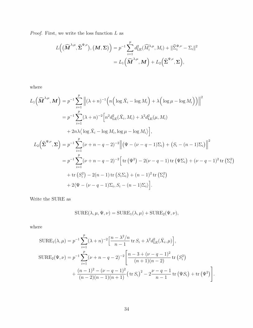
Consider the loss function

L((M , Σ), (M ,Σ)

)= p−1

p∑i=1

d2LE(Mi,Mi) + p−1

p∑i=1

‖Σi − Σi‖2

= L1(M ,M ) + L2(Σ,Σ).

10

Its induced risk function is given by

R((M , Σ), (M ,Σ)

)= p−1

p∑i=1

Ed2LE(Mi,Mi) + E‖Σi − Σi‖2

= p−1(λ+ n)−2

p∑i=1

[ntrΣi + λ2d2

LE(µ,Mi)]

+ p−1

p∑i=1

(ν + n− q − 2)−2[(n− 1 + (ν − q − 1)2

)tr(Σ2

i )

− 2(ν − q − 1)tr(ΨΣi) + (n− 1)(trΣi)2 + tr(Ψ2)

]with the detailed derivation given in the supplemental material. The SURE for this risk

function is

SURE(λ,Ψ, ν, µ) = p−1

{p∑i=1

(λ+ n)−2[n− λ2/n

n− 1trSi + λ2d2

LE(Xi, µ)]

+ (ν + n− q − 2)−2[n− 3 + (ν − q − 1)2

(n+ 1)(n− 2)tr(S2

i )

+(n− 1)2 − (ν − q − 1)2

(n− 1)(n+ 1)(n− 2)

(trSi

)2 − 2ν − q − 1

n− 1tr(ΨSi) + tr(Ψ2)

]}with the detailed derivation given in the supplemental material.

The hyperparameter vector (λ,Ψ, ν, µ) is estimated by minimizing SURE(λ,Ψ, ν, µ), and

the resulting shrinkage estimators of Mi and Σi are obtained by plugging in the minimizing

vector into (9). Note that this is a non-convex optimization problem and for such problems,

the convergence relies heavily on the choice of the initialization. We suggest the following

initialization, which is discussed in the supplemental material:

µ0 = exp

(p−1

p∑i=1

log Xi

)

λ0 =np−1

∑pi=1 d

2LE(Xi, µ0)

np(n−1)

∑pi=1 trSi − p−1

∑pi=1 d

2LE(Xi, µ0)

ν0 =q + 1

n−q−2p2q(n−1)

tr[(∑p

i=1 Si)(∑p

i=1 S−1i

)]− 1

+ q + 1

Ψ0 =ν0 − q − 1

p(n− 1)

p∑i=1

Si.

In all our experiments, the algorithm converged in less than 20 iterations with the suggested

initialization. This concludes the description of our estimators of the unknown means and

11

covariance matrices. Theorem 5 below states that SURE(λ,Ψ, ν, µ) approximates the true

loss L((M

λ,µ, Σ

Ψ,ν),(M ,Σ

))well in the sense that the difference between the two random

variables converges to 0 in probability as p→∞. Additionally, Theorem 6 below shows that

the estimators of M and Σ obtained by minimizing SURE(λ,Ψ, ν, µ) are asymptotically

optimal in the class of estimators of the form (9).



i=1

(tr Σi

)4<∞,


i=1 MTi ΣiMi <∞,



Then

supλ>0,ν>q+1,‖Ψ‖≤max1≤i≤p ‖Si‖,‖log µ‖≤max1≤i≤p ‖log Xi‖

∣∣∣SURE(λ,Ψ, ν, µ)−L((M

λ,µ, Σ

Ψ,ν), (M ,Σ)

)∣∣∣ prob−→ 0 as p→∞.

Note that the optimization has some constraints. However, in practice, with proper

initialization as suggested earlier, the constraints on Ψ and µ can be safely ignored. The

reason is that, for Ψ and µ far from Si’s and Xi respectively, the value of SURE will be large.

The constraints on λ and ν can easily be handled by standard constrained optimization

algorithms, e.g. L-BFGS-B (Byrd et al. 1995).

Theorem 4 If assumptions (i), (ii), and (iii) in Theorem 5 hold, then

limp→∞

[R((M

SURE, Σ

SURE), (M ,Σ)

)−R

((M

λ,µ, Σ

Ψ,ν), (M ,Σ)

)]≤ 0.

Note that in all the above theorems, we consider the asymptotic regime p → ∞ while

the size of the SPD matrix N is held fixed. The main reason for fixing the size of the SPD

matrix is that in our application, namely the DTI analysis, the size of the diffusion tensors

is always 3× 3, because the diffusion magnetic resonance images are 3-dimensional images.

However, the number of voxels p can increase as they are determined by the resolution of

the acquired image which can increase due to advances in medical imaging technology. This

12

is different from the usual high dimensional covariance matrix estimation problem in which

the size of the covariance matrix is allowed to grow.

Remark: The proofs of Theorems 1 and 2 in Yang & Vemuri (2019) use arguments

similar to those that already exist in the literature, and in that sense they are not very

difficult. In contrast, the proofs of our Theorems 5 and 6 above do not proceed along

familiar lines. Indeed, they are rather complicated, the difficulty being that bounding the

moments of Wishart matrices or the moments of trace of Wishart matrices is nontrivial

when the orders of the required moments are higher than two. We present these proofs in

the supplementary document.

3.3 Tweedie’s Formula for F Statistics

One of the motivations for the development of our approach for estimating M and Σ is a

problem in neuroimaging involving detection of differences between a patient group and a

control group. The problem can be stated as follows. There are nx patients in a disease

group and ny normal subjects in a control group. We consider a region of the brain image

consisting of p voxels. As explained in section 4.2, the local diffusional property of water

molecules in the human brain is of clinical importance and it is common to capture this

diffusional property at each voxel in the diffusion magnetic resonance image (dMRI) via a

zero-mean Gaussian with a 3×3 covariance matrix. Using any of the existing state-of-the-art

dMRI analysis techniques, it is possible to estimate, from each patient image, the diffusion

tensor Mi corresponding to voxel i, for i = 1, . . . , p. Let M(1)i and M

(2)i denote the diffusion

tensors corresponding to voxel i for the disease and control groups respectively. The goal is

to identify the indices i for which the difference between M(1)i and M

(2)i is large. The model

we consider is

Xijind∼ LN(M

(1)i ,Σi), i = 1, . . . , p, j = 1, . . . , nx,

Yijind∼ LN(M

(2)i ,Σi), i = 1, . . . , p, j = 1, . . . , ny.

In this work, we compute the Hotelling T 2 statistic for each i = 1, . . . , p as a measure of

the difference between M(1)i and M

(2)i . The Hotelling T 2 statistic for SPD matrices has been

13

proposed by Schwartzman et al. (2010) and is given by

t2i =(˜Xi − ˜Yi)T[( 1

nx+

1

ny

)Si

]−1(˜Xi − ˜Yi) (10)

where Xi and Yi are the FMs of {Xij}j and {Yij}j and Si = (nx + ny − 2)−1(S

(1)i + S

(2)i

)is

the pooled estimate of Σi where S(1)i and S

(2)i are computed using (8). Since the Xij’s and

Yij’s are Log-normally distributed, one can easily verify that the sampling distribution of t2i

is given byν − q − 1

νqt2i

ind∼ Fq,ν−q−1,λi

where ν = nx + ny − 2 is a degrees of freedom parameter (recall that q = N(N + 1)/2).

Note that we make the assumption that the covariance matrices for the two groups are the

same, i.e. Σ(1)i = Σ

(2)i = Σi. Similar results can be obtained for the unequal covariance

case, but with more complicated expressions for the T 2 statistics and the degrees of freedom

parameters. The λi’s are the non-centrality parameters for the non-central F distribution

and are given by

λi =( 1

nx+

1

ny

)(M

(1)i − M

(2)i

)TΣ−1i

(M

(1)i − M

(2)i

).

These non-centrality parameters can be interpreted as the (squared) differences between M(1)i

and M(2)i , and they are the parameters we would like to estimate using the statistics (10)

computed from the data. Then, based on the estimates λi, we select those i’s with large

estimates, say the largest 1% of all λi. However, the process of selection from the computed

estimates introduces a selection bias (Dawid 1994). The selection bias comes from the fact

that it is possible to select some indices i’s for which the actual λi’s are not large but the

random errors are large, so that the estimates λi are pushed away from the true parameters

λi. There are several ways to correct this selection bias, and Efron (2011) proposed to use

Tweedie’s formula for such a purpose.

Tweedie’s formula was first proposed by Robbins (1956), and we review this formula

here in the context of the classical normal means problem, which is stated as follows. We

observe Ziind∼ N(µi, σ

2), i = 1, . . . , p, where the µi’s are unknown and σ2 is known, and the

goal is to estimate the µi’s. In the empirical Bayes approach to this problem we assume

that µi’s are iid according to some distribution G. The marginal density of the Zi’s is then

14

f(z) =∫φσ(z − µ) dG(µ), where φσ is the density of the N(0, σ2) distribution. With this

notation, if G is known (so that f is known), the best estimator of µi (under squared error

loss) is the so-called Tweedie estimator given by

µi = Zi + σ2f′(Zi)

f(Zi).

A feature of this estimator is that it depends on G only through f , and this is desirable

because it is fairly easy to estimate f from the Zi’s (so we don’t need to specify G). Another

interesting observation about this estimator is that µi is shrinking the MLE µMLEi = Zi and

can be viewed as a generalization of the James-Stein estimator, which assumes µiiid∼ N(0, λ)

with unknown λ. The Tweedie estimator can be generalized to exponential families. Suppose

that Zi|ηiind∼ fηi(z) = exp(ηiz − φ(ηi))f0(z), and the prior for φ is G. Then the Tweedie

estimator for ηi is

ηi = l′(Zi)− l′0(Zi),

where l(z) = log∫fη(z) dG(η) is the log of the marginal likelihood of the Zi’s and l0(z) =

log f0(z).

Although this formula is elegant and useful, it applies only to exponential families. Re-

cently, Du & Hu (2020) derived a Tweedie-type formula for non-central χ2 statistics, for

situations where one is interested in estimating the non-centrality parameters. Suppose

Zi|λiind∼ χ2

ν,λiand λi

iid∼ G. Then,

E(λi|Zi) =[(Zi − ν + 4) + 2Zi

( 2l′′ν(Zi)

1 + 2l′ν(Zi)+ l′ν(Zi)

)](1 + 2l′ν(Zi)

), (11)

where lν(·) is the marginal log-likelihood of the Zi’s (see Theorem 1 in Du & Hu (2020)).

For our situation, if we define Zi = [(ν − q − 1)/νq]t2i , then

Zi|λiind∼ Fq,ν−q−1,λi

(recall that ν = nx +ny− 2). Assume that the λi’s are iid according to some distribution G.

We would now like to address the problem of how to obtain an empirical Bayes estimate of λi.

Let Φν1,ν2,λ be the cumulative distribution function (cdf) of the non-central F distribution,

Fν1,ν2,λ, and let Φν,λ be the cdf of the non-central χ2 distribution, χ2ν,λ. Then the transformed

variable Yi = Φ−1ν1,λi

(Φν1,ν2,λi(Zi)) follows a non-central χ2 distribution with degrees of freedom

15

parameter ν1 and non-centrality parameter λi, and we note that when ν2 is large, Φν1,ν2,λi and

Φν1,λi are nearly equal, so that this quantile transformation is nearly the identity. However,

the transformation depends on λi, which is the parameter to be estimated, so we propose

the following iterative algorithm for estimating E(λi|Zi). Let λ(t)i be the estimate of λi at

the t-th iteration. Then, our iterative update of λi is given by

λ(t+1)i =

[(Y

(t)i − ν1 + 4) + 2Y

(t)i

( 2l′′ν1(Y(t)i )

1 + 2l′ν1(Y(t)i )

+ l′ν1(Y(t)i ))](

1 + 2l′ν1(Y(t)i )),

where Y(t)i = Φ−1

ν1,λ(t)i

(Φν1,ν2,λ

(t)i

(Zi)), ν1 = q, and ν2 = ν − q − 1. Now the marginal log-

likelihood lν1(y) is not available since the prior G for λi is unknown. There are several

ways to estimate the marginal density of the Y(t)i ’s. One of these is through kernel density

estimation. However, the iterative formula involves the first and second derivatives of the

marginal log-likelihood, and estimates of the derivatives of a density produced through kernel

methods are notoriously unstable (see Chapter 3 of Silverman (1986)). There exist different

approaches to deal with this problem (see Sasaki et al. (2016) and Shen & Ghosal (2017)).

Here we follow Efron (2011) and postulate that lν1 is well approximated by a polynomial of

degree K, and write lν1(y) =∑K

k=0 βkyk. The coefficients βk, k = 1, . . . , K, can be estimated

via Lindsey’s method (Efron & Tibshirani 1996), which is a Poisson regression technique for

(parametric) density estimation; the coefficient β0 is determined by the requirement that

fν1(y) = exp(lν1(y)) integrates to 1. The advantage of Lindsey’s method over methods

that use kernel density estimation is that it does not require us to estimate the derivatives

separately, since l′ν1(y) =∑K

k=1 kβkyk−1 and l′′ν1(y) =

∑Kk=2 k(k−1)βky

k−2. In our experience,

with l′ν1 and l′′ν1 estimated in this way, if we initialize the scheme by setting λ(0)i to be the

estimate of λi given by Du & Hu (2020) procedure, then the algorithm converges in less than

10 iterations.

4 Experimental Results

In this section, we describe the performance of our methods on two synthetic data sets and

on two sets of real data acquired using diffusion magnetic resonance brain scans of normal

(control) subjects and patients with Parkinson’s disease. For the synthetic data experi-

16

ments, we show that (i) the proposed shrinkage estimator for the FM (SURE.Full-FM; with

simultaneous estimation of the covariance matrices) outperforms the sample FM (FM.LE)

and the shrinkage estimator proposed by Yang & Vemuri (2019) (SURE-FM; with fixed co-

variance matrices) (section 4.1.1); (ii) the shrinkage estimates of the differences capture the

regions that are significantly different between two groups of SPD matrix-valued images

(section 4.1.2). For the real data experiments, we demonstrate that (iii) the SURE.Full-

FM provides improvement over the two competing estimators (FM.LE, and SURE-FM) for

computing an atlas (templates) of diffusion tensor images acquired from human brains (sec-

tion 4.2.1); (iv) the proposed shrinkage estimator for detecting group differences is able to

identify the regions that are different between patients with Parkinson’s disease and control

subjects (section 4.2.2). Details of these experiments will be presented subsequently.

4.1 Synthetic Data Experiments

We present two synthetic data experiments here to show that the proposed shrinkage esti-

mator, SURE.Full-FM, outperforms the sample FM and SURE-FM and that the shrinkage

estimates of the group differences can accurately localize the regions that are significantly

different between the two groups.

4.1.1 Comparison Between SURE.Full-FM and Competing Estimators

Using generated noisy SPD fields (P3) as data, here we present performance comparisons of

four estimators of M : (i) SURE.Full-FM, which is the proposed shrinkage estimator, (ii)

SURE-FM proposed by Yang & Vemuri (2019) which assumes known covariance matrices

and (iii) the MLE, which is denoted by FM.LE, since by proposition 1 it is the FM based on

the Log-Euclidean metric. The synthetic data are generated according to (7). Specifically,

we set µ = I3, Ψ = I6, and n = 10, and we vary the variance λ and the degree of freedom ν of

the prior distribution as follows: λ = 10, 50, and ν = 15, 30. Figure 1 depicts the relationship

between the average loss (averaged over m = 1000 replications) and the dimension p under

varying conditions for the four estimators. Note that since the covariance matrices Σi’s are

unknown in our synthetic experiment and (n − 1)−1Si is an unbiased estimate for Σi, the

17

Ai’s in (6) can be unbiasedly estimated by [(n− 1)q]−1 trSi.

0.02

0.04

0.06

0.08

Aver

age

Loss

= 10.0

EstimatorFM.LE (MLE)

SURE-FM

SURE.Full-FM

= 50.0

=15.0

0 50 100 150 200

0.01

0.02

0 50 100 150 200Spatial Dimension (p)

=30.0

Figure 1: Average loss for the three estimators. Results for varying λ and degree of freedom

ν are shown across the columns and rows, respectively. Note that in the bottom two panels,

the line corresponding to FM.LE is essentially the same as the SURE.FM, but is barely

visible.

As is evident from Figure 1, for large λ the gains from using SURE.Full-FM are greater.

This observation is in accordance with our intuition, which is that for large λ, the Mi’s are

clustered, and it is beneficial to shrink the MLEs of the Mi’s towards a common value. The

main difference between SURE-FM and SURE.Full-FM is that the former requires knowledge

of the Σi’s and in general such information is not available, and estimates for the Σi’s are

needed to compute the SURE-FM. Hence the performance of SURE-FM depends heavily on

how good the estimates for the Σi’s are. In our synthetic data experiment, we consider the

unbiased estimate Ai = [(n− 1)q]−1 trSi for SURE-FM. In this case, the prior mean for Σi

is E(Σi) = (ν− q−1)−1Iq for which the assumption Σi = AiI seems reasonable. For large ν,

the Ai’s are closer to zero, which results in a smaller shrinkage effect (this can be observed

in Figure 1, where we see that SURE-FM is almost identical to FM.LE for ν = 30). Note

that even if the assumption Σi = AiI is not severely violated, our estimator still outperforms

18

SURE-FM by a large margin.

On the other hand, we can fix λ and ν to see how different choices of µ and Ψ affect the

performance of our shrinkage estimator SURE.Full-FM. To do this, we fix n = 10, λ = 10,

and ν = 15 (so that we can compare with the top-left panel of Figure 1). We consider

µ = diag(2, 0.5, 0.5) and Ψij = 0.5|i−j|. The result is shown in Figure 2. The top-left panel

of Figure 1 shows that when µ = I and Ψ = I, there is no difference between SURE-FM and

SURE.Full-FM, but Figure 2 shows that when one of µ and Ψ is not identity, our shrinkage

estimator outperforms SURE-FM. For different choices of λ and ν, the improvement will be

more significant, following the trend we observed in Figure 1.

0 50 100 150 200

0.04

0.05

0.06

0.07

Aver

age

Loss

= diag(2, 0.5, 0.5), = I6

EstimatorFM.LE (MLE)

SURE-FM

SURE.Full-FM

0 50 100 150 200Spatial Dimension (p)

= I3, = [0.5|i j|]i, j

Figure 2: Average losses for the four estimators. The left panel assumes µ = diag(2, 0.5, 0.5)

and Ψ = I and the right panel assumes µ = I and Ψij = 0.5|i−j|.

4.1.2 Differences Between Two Groups of SPD-Valued Images

In this subsection, we demonstrate the method proposed in section 3.3 for evaluating the

difference between two groups of SPD-valued images. For this synthetic data experiment, we

use P2, the manifold of 2× 2 SPD matrices, since it is easy to visualize these matrices. For

the visualization, we represent each 2×2 SPD matrix of the SPD-valued image by an ellipse

with the two eigenvectors as the axes of the ellipse and the two eigenvalues as the width and

height along the corresponding axes respectively. The data are generated as follows. Given

19

nk, M(k)i , σ2

i , k = 1, 2, i = 1, . . . , p, generate

Xijind∼ LN(M

(1)i , σ2

i I), j = 1, . . . , n1,

Yijind∼ LN(M

(2)i , σ2

i I), j = 1, . . . , n2.

We generate n1 = n2 = 30 P2-valued images for the two groups, and the size of each P2-

valued image is 20 × 20, which gives p = 20 × 20 = 400. For the variances σj, we consider

a low variance scenario σiiid∼ U(0.1, 0.3) and a high variance scenario σi

iid∼ U(0.3, 0.8). The

means M(k)i are depicted visually in Figure 3 (in the form of images with ellipses instead of

gray values at each pixel), and the region in which the means are different is the top-right

corner, containing a quarter of the pixels; this is the ‘ground truth’ data.

(a) Group 1 (b) Group 2

Figure 3: The mean P2-valued images M(k)i , k = 1, 2, used to generate random P2-valued

images for the two groups. The vertical ellipse represents the matrix diag(0.3, 1) and the

horizontal ellipse represents the matrix diag(1, 0.3).

As described in section 3.3, we first compute the Hotelling T 2 statistic from {Xij}n1j=1 and

{Yij}n2j=1 for each i and transform each of them to the F statistic. Now we have p non-central

F statistics, fiind∼ Fν1,ν2,λi , i = 1, . . . , p, where ν1 = q = 3, and ν2 = n1 + n2 − 2 − q − 1 =

n1+n2−6. With the resulting F statistics, we can apply the algorithm described in section 3.3

to estimate the non-centrality parameters (at each location), and for the estimation of the

marginal log likelihood, we adopt Lindsey’s method to fit a polynomial of degree K = 5 to the

20

log-likelihood lν1 . We have experimented using different values of K, and we found that the

results are robust to changes in K, at least for relatively small K. In our experiments, we set

n1 = n2 = 30. As we can see from Figure 3, we expect the method to yield large values on the

top-right corner of the image and small values for the rest of the matrix-valued image (field).

We compare the proposed estimator λTweediei to the estimator λMOM

i = max(ν1(ν2−2)

ν2fi−ν1, 0

),

which is obtained by the method of moments (MOM) and truncated at 0, and also compare

them for different σ2i ’s. Note that we choose to compare with the MOM estimator instead

of the MLE for two reasons: (i) the MLE for the non-centrality parameter of non-central

F distribution is expensive to compute, and (ii) the MOM is commonly used as a standard

for comparison, see for example Kubokawa et al. (1993). As we can see from the results,

there are more black spots (which indicate no difference) in the top-right corner for the

MOM estimates than the Tweedie-adjusted estimates. These show that the Tweedie-adjusted

estimator allows us to capture the true region of difference better than the MOM estimator

does, especially for large σ2i ’s. This is due to the presence of the shrinkage effect in Tweedie’s

formula.

4.2 Real Data Experiments

In this section, we present two real data experiments involving dMRI data sets. The diffu-

sion MRI data used here is available for public access via https://pdbp.ninds.nih.gov/

our-data. dMRI is a diagnostic imaging technique that allows one to non-invasively probe

the axonal fiber connectivity in the body by making the magnetic resonance signal sensitive

to water diffusion through the tissue being imaged. In dMRI, the water diffusion is fully char-

acterized by the probability density function (PDF) of the displacement of water molecules,

called the ensemble average propagator (EAP) (Callaghan 1993). A simple model that has

been widely used to describe the displacement of water molecules is a zero mean Gaussian;

its covariance matrix defines the diffusion tensor and characterizes the diffusivity functional

locally. The diffusion tensors are 3 × 3 SPD matrices and hence have 6 unique entries that

need to be determined. Thus, the diffusion imaging technique employed in this case involves

the application of at least 6 diffusion sensitizing magnetic gradients for acquisition of full

3D MR images (Basser et al. 1994). This dMRI technique is called diffusion tensor imaging

21

https://pdbp.ninds.nih.gov/our-data

https://pdbp.ninds.nih.gov/our-data

0.0 2.5 5.0 7.5 10.0 12.5 15.0 17.50.0

2.5

5.0

7.5

10.0

12.5

15.0

17.5

20

40

60

80

100

(a) λTweedie, σiiid∼ U(0.1, 0.3)

0.0 2.5 5.0 7.5 10.0 12.5 15.0 17.50.0

2.5

5.0

7.5

10.0

12.5

15.0

17.5

0

2

4

6

8

10

(b) λTweedie, σiiid∼ U(0.3, 0.8)

0.0 2.5 5.0 7.5 10.0 12.5 15.0 17.50.0

2.5

5.0

7.5

10.0

12.5

15.0

17.5

0

20

40

60

80

100

120

(c) λMOM, σiiid∼ U(0.1, 0.3)

0.0 2.5 5.0 7.5 10.0 12.5 15.0 17.50.0

2.5

5.0

7.5

10.0

12.5

15.0

17.5

0

2

4

6

8

10

12

(d) λMOM, σiiid∼ U(0.3, 0.8)

Figure 4: Comparison between the proposed shrinkage estimates and MOM estimates of the

non-centrality parameters.

(DTI). Some practical techniques for estimating the diffusion tensors and population mean

of diffusion tensors accurately can be found in Wang & Vemuri (2004), Chefd’Hotel et al.

(2004), Fletcher & Joshi (2004), Alexander (2005), Zhou et al. (2008), Lenglet, Rousson &

Deriche (2006), and Dryden et al. (2009).

DTI has been the de facto non-invasive dMRI diagnostic imaging technique of choice in

the clinic for a variety of neurological ailments. After fitting/estimating the diffusion tensors

at each voxel, scalar-valued or vector-valued measures are derived from the diffusion tensors

for further analysis. For instance, fractional anisotropy (FA) is a scalar-valued function

of the eigenvalues of the diffusion tensor and it was found that FA was reduced in the

22

neuro-anatomical structure called the Substantia Nigra in patients with Parkinson’s disease

compared to control subjects (Vaillancourt et al. 2009). In Schwartzman et al. (2008), the

authors proposed to use the principal direction, which is the eigenvector corresponding to

the largest eigenvalue of the diffusion tensor, to represent the entire tensor; the principal

direction contains directional information that any scalar measures such as the FA does not

and hence, might be able to capture some subtle differences in the anatomical structure of

the brain. In this work, we use the full diffusion tensor which captures both the eigen-values

and eigen-vectors, in order to assess the changes caused by pathologies to the underlying

tissue micro-architecture revealed via dMRI.

4.2.1 Estimation of the Motor Sensory Tracts of Patients with Parkinson’s Dis-

ease

In this section, we demonstrate the performance of SURE.Full-FM on the dMRI scans of

human brain data acquired from 50 patients with Parkinson’s disease and 44 control (normal)

subjects. The diffusion MRI acquisition parameters were as follows: repetition time =

7748ms, echo time = 86ms, flip angle = 90◦, number of diffusion gradients = 64, field of

view = 224 × 224 mm, in-plane resolution = 2 mm isotropic, slice-thickness = 2 mm, and

SENSE factor = 2. All the dMRI data were pre-registered into a common coordinate frame

prior to any further data processing.

The motor sensory area fiber tracts (M1 fiber tracts) are extracted from each patient

of the two groups using the FSL software (Behrens et al. 2007). The size (length) of each

tract is 33 voxels for the left hemisphere tract and 34 voxels for the right hemisphere tract,

respectively. Diffusion tensors are then fitted to each of the voxels along each of the tracts to

obtain p = 33 (p = 34) 3× 3 SPD matrices. We then compute the Log-Euclidean FM tract

for each group. The FM tract here also has 33 (34) diffusion tensors along the tract. We

will use these FMs computed from the full population of each group as the ‘ground truth’;

thus, the underlying distribution in this experiment is the empirical distribution formed by

the observed data, i.e. the 33 (34) SPD matrices. Then, we randomly draw a subsample of

size n = 10, 20, 50, 100 (with replacement) respectively from each group and compute the

SURE.Full-FM (our proposed estimator) and the three competing estimators (FM.LE and

23

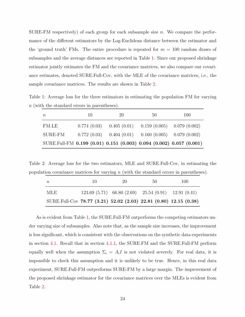
SURE-FM respectively) of each group for each subsample size n. We compare the perfor-

mance of the different estimators by the Log-Euclidean distance between the estimator and

the ‘ground truth’ FMs. The entire procedure is repeated for m = 100 random draws of

subsamples and the average distances are reported in Table 1. Since our proposed shrinkage

estimator jointly estimates the FM and the covariance matrices, we also compare our covari-

ance estimates, denoted SURE.Full-Cov, with the MLE of the covariance matrices, i.e., the

sample covariance matrices. The results are shown in Table 2.

Table 1: Average loss for the three estimators in estimating the population FM for varying

n (with the standard errors in parentheses).

n 10 20 50 100

FM.LE 0.774 (0.03) 0.405 (0.01) 0.159 (0.005) 0.079 (0.002)

SURE-FM 0.772 (0.03) 0.404 (0.01) 0.160 (0.005) 0.079 (0.002)

SURE.Full-FM 0.199 (0.01) 0.151 (0.003) 0.094 (0.002) 0.057 (0.001)

Table 2: Average loss for the two estimators, MLE and SURE.Full-Cov, in estimating the

population covariance matrices for varying n (with the standard errors in parentheses).

n 10 20 50 100

MLE 123.69 (5.71) 66.80 (2.69) 25.54 (0.91) 12.91 (0.41)

SURE.Full-Cov 78.77 (3.21) 52.02 (2.03) 22.81 (0.80) 12.15 (0.38)

As is evident from Table 1, the SURE.Full-FM outperforms the competing estimators un-

der varying size of subsamples. Also note that, as the sample size increases, the improvement

is less significant, which is consistent with the observations on the synthetic data experiments

in section 4.1. Recall that in section 4.1.1, the SURE.FM and the SURE.Full-FM perform

equally well when the assumption Σi = AiI is not violated severely. For real data, it is

impossible to check this assumption and it is unlikely to be true. Hence, in this real data

experiment, SURE.Full-FM outperforms SURE-FM by a large margin. The improvement of

the proposed shrinkage estimator for the covariance matrices over the MLEs is evident from

Table 2.

24

4.2.2 Tweedie-Adjusted Estimator as an Imaging Biomarker

Finally, we apply the shrinkage estimator proposed in section 3.3 to identify the regions that

are significantly distinct in diffusional properties (as captured via diffusion tensors) between

patients with Parkinson’s disease and control subjects. In this experiment, the dataset

consists of DTI scans of 46 patients with Parkinson’s disease and 24 control subjects. To

identify the differences between the two groups, we use the DTI of the whole brain, which

contains p = 112×112×60 voxels, without pre-selecting any region of interest. The diffusion

tensors are fitted at each voxel across the whole brain volume. The goal of this experiment

is to see if we are able to automatically identify the regions capturing the large differences

between the Parkinson’s disease group and control groups and qualitatively validate our

findings against what is expected by expert neurologists. In this context, Prodoehl et al.

(2013) observed that the region most affected by Parkinson’s disease is the Substantia Nigra,

which is contained in the Basal Ganglia region of the human brain.

After computing both the Tweedie-adjusted estimates and the MOM estimates of the non-

centrality parameters, we select voxels with the largest 1% estimates of the non-centrality

parameters and mark those voxels in bright red. (Note that there are other ways to determine

the threshold for the selection, for example by using the false discovery rate (FDR) in

hypothesis testing problems. However, this is beyond the scope of this paper and we refer

the reader to Schwartzman (2008) for interesting work on FDR analysis for DTI datasets.)

These voxels are where the large differences between Parkinson’s disease group and control

group are observed. The results are shown in Figure 5. For a better visualization, we

threshold the estimates by the top 1%. Note that, to take into account the spatial structure,

we apply a 4×4×4 average mask to smooth the result. This smoothing may also be achieved

by incorporating spatial regularization term in the expression for SURE (??). However, the

ensuing analysis becomes much more complicated and will be addressed in our future work.

From the results, we can see that the shrinkage effect of our Tweedie-adjusted estimate

successfully corrects the selection bias and produces more accurate identification of the af-

fected regions. Our method is able to capture the Substantia Nigra, which is the region

known to be affected by Parkinson’s disease. Notably, our method did not point to the ap-

25

parently spurious and isolated regions selected by the MOM estimator (the tiny red spots in

Figure 5(a)). We also mention that the past research using FA-based analysis did not re-

port the Internal Capsule as a region affected by Parkinson’s disease. We suspect that this

discrepancy is due to the fact that FA discards the directional information of the diffusion

tensors while we use the full diffusion tensor which contains the directional information.

We plan to conduct a large-scale experiment in our future work to see if this observation

continues to hold.

(a) MOM estimates (b) Tweedie-adjusted estimates

Figure 5: Differences between Parkinson’s disease and control groups are superimposed on

dMRI scans of a randomly-chosen Parkinson’s disease patient and indicated in red.

5 Discussion and Conclusions

In this work, we presented shrinkage estimators for the mean and covariance of the Log-

Normal distribution defined on the manifold PN of N×N SPD matrices. We also showed that

the proposed shrinkage estimators are asymptotically optimal in a large class of estimators

including the MLE. The proposed shrinkage estimators are in closed form and resemble

(in form) the James-Stein estimator in Euclidean space Rp. We demonstrated that the

proposed shrinkage estimators outperform the MLE via several synthetic data examples

and real data experiments using diffusion tensor MRI datasets. The improvements of the

proposed shrinkage estimators are significant especially in the small sample size scenarios,

which is very pertinent to medical imaging applications.

26

Our work reported here is however based on the Log-Euclidean metric, and one of the

drawbacks of this metric is that it is not affine (GL) invariant, which is a desired property

in some applications. Unfortunately, the derivation of the shrinkage estimators under the

GL-invariant metric is challenging due to the fact that there is no closed-form expression

for some elementary quantities such as the sample FM which makes it almost impossible to

derive the corresponding SURE. Our future research efforts will focus on developing a general

framework for designing shrinkage estimators that are applicable to general Riemannian

manifolds.

For applications in localizing the regions of the brain where the two groups differ, our

approach already works well, but it can potentially be improved if we take into account the

fact that neighboring voxels within a region are close under some measure of similarity. For

instance, M(k)i and M

(k)j should be close if voxels i and j are close. Currently, our approach

is to apply a spatial smoother to the Tweedie-adjusted estimates. Instead, the improvement

can be achieved by imposing regularization constraints, e.g. a spatial process prior, in the

proposed framework. However, the ensuing analysis becomes rather complicated and will be

the focus of our future efforts.

27

Supplement to “An Empirical BayesApproach to Shrinkage Estimation on theManifold of Symmetric Positive-Definite

Matrices”

Abstract

In this supplement, we provide the technical details in section 3.2 of the main paper,

including the derivation of the risk function and the SURE, the proofs for Theorem

5 and 6, and the implementation details for minimizing SURE. The notation used in

this supplement is the same as in the main paper.

1 Preliminary

Before presenting the proofs, we review the following elementary results for both multivariate

normal distributions and Wishart distributions which are use extensively in the proofs. Let

X ∼ Np(µ,Σ). Then

E‖X − c‖2 = tr Σ + ‖µ− c‖2

E‖X − c‖4 = (tr Σ)2 + 2 tr(Σ2) + 4(µ− c)TΣ(µ− c) + 2‖µ− c‖2 tr Σ + ‖µ− c‖4

where c ∈ Rp. For X ∼ LN(M,Σ),

Ed2LE(X,C) = tr Σ + d2

LE(M,C)

Ed4LE(X,C) = (tr Σ)2 + 2 tr(Σ2) + 4(M − C)TΣ(M − C) + 2d2

LE(M,C) tr Σ + d4LE(M,C)

where C ∈ PN . These results can be easily obtained from the definition of the Log-Normal

distribution.

Let Y be a p×p symmetric matrix with eigenvalues λ1, . . . , λp and let κ = (k1, . . . , kp) be

a (non-increasing) partition of a positive integer k, i.e. k1 ≥ k2 ≥, . . . ,≥ kp and∑p

i=1 ki = k

where the ki’s are non-negative integers. The zonal polynomial of Y corresponding to κ,

denoted by Cκ(Y ), is a symmetric, homogeneous polynomial of degree k in the eigenvalues

28

λ1, . . . , λp. One of the properties of the zonal polynomials is that(

trY)k

=∑

κCκ(Y ). For

a more precise definition of the zonal polynomial and its calculations, we refer the readers

to Ch. 7 of Muirhead (1982). The following lemma is essential in our work.

Lemma 1 (Muirhead (1982), Corollary 7.2.4) If Y is positive definite, then Cκ(Y ) > 0 for

all partitions κ.

The jth elementary symmetric function of Y , denoted by trj Y , is the sum of all principal

minors of order j of the matrix Y . For the case of j = 1, tr1 Y =∑p

i=1 λi = trY , and for the

case of j = 2, tr2 Y =∑

i<j λiλj. The definition gives rise to the following identities which

are useful in the proofs

(trY )2 = tr(Y 2) + 2 tr2 Y (12)

(trY )4 = (tr(Y 2))2 + 4 tr(Y 2) tr2 Y + 4(tr2 Y )2

= tr(Y 4) + 2 tr2 Y2 + 2(tr2 Y )(trY )2 (13)

For S ∼Wishartp(Σ, ν), the kth moment, k = 0, 1, 2, . . . of trS is given by

E(trS)k = 2k∑κ

(ν2

)κCκ(Σ) (14)

where

(a)κ =

p∏i=1

(a− i− 1

2

)ki

is called the generalized hypergeometric coefficient and

(a)ki = a(a+ 1) . . . (a+ ki − 1), (a)0 = 1

(Gupta & Nagar (2000), Theorem 3.3.23). Next, we review some elementary results for the

Wishart distribution:

ES = νΣ

ES2 = ν(ν + 1)Σ2 + ν(tr Σ)Σ

E trk S = ν(ν − 1) · · · (ν − k + 1) trk Σ

E(trS)2 = ν(ν + 2)(tr Σ)2 − 4ν tr2 Σ = ν2(tr Σ)2 + 2ν tr(Σ2).

These results can be found in Gupta & Nagar (2000)(p. 99 and p. 106).

29

2 Derivation of the Risk Function and the SURE

Recall that the loss function is L((M , Σ), (M ,Σ)

)= p−1

∑pi=1 d

2LE(Mi,Mi)+p−1

∑pi=1 ‖Σi−

Σi‖2 = L1(M ,M ) + L2(Σ,Σ). Write R((M , Σ), (M ,Σ)

)= EL1(M ,M ) + EL2(Σ,Σ) =

R1(M ,M ) +R2(Σ,Σ). Then

R1(M ,M ) = p−1

p∑i=1

Ed2LE(Mi,Mi)

= p−1

p∑i=1

[ n2

(λ+ n)2Ed2

LE(Xi,Mi) +λ2

(λ+ n)2d2

LE(µ,Mi)]

= p−1(λ+ n)−2

p∑i=1

[ntrΣi + λ2d2

LE(µ,Mi)]

and

R2(Σ,Σ) = p−1

p∑i=1

(ν + n− q − 2)−2E‖(Ψ− (ν − q − 1)Σi) + (Si − (n− 1)Σi)‖2

= p−1

p∑i=1

(ν + n− q − 2)−2[E tr(S2

i )− 2(n− 1)E tr(SiΣi) + (n− 1)2 tr(Σ2i )

+ tr(Ψ2)− 2(ν − q − 1) tr(ΨΣi) + (ν − q − 1)2 tr(Σ2i )]

= p−1

p∑i=1

(ν + n− q − 2)−2[n(n− 1) tr(Σ2

i ) + (n− 1)(tr Σi)2 − 2(n− 1)2 tr(Σ2

i )

+ (n− 1)2 tr(Σ2i ) + tr(Ψ2)− 2(ν − q − 1) tr(ΨΣi) + (ν − q − 1)2 tr(Σ2

i )]

= p−1

p∑i=1

(ν + n− q − 2)−2[(n− 1 + (ν − q − 1)2

)tr(Σ2

i )

− 2(ν − q − 1)tr(ΨΣi) + (n− 1)(trΣi)2 + tr(Ψ2)

].

To obtain the SURE for this risk function, we first have to find unbiased estimates of the

quantities tr Σi, d2LE(µ,Mi), tr(Σ2

i ), tr(ΨΣi), and (tr Σi)2. With the results provided in

30

Section 1, it is easy to verify the following equations:

tr Σi = E((n− 1)−1 trSi

)tr(ΨΣi) = E

((n− 1)−1 tr(ΨSi)

)(tr Σi)

2 = E( n(trSi)

2 − 2 trS2i

(n− 1)(n+ 1)(n− 2)

)tr Σ2

i = E((n− 1) trS2

i − (trSi)2

(n− 1)(n+ 1)(n− 2)

)d2

LE(µ,Mi) = E(d2

LE(Xi, µ)− trSin(n− 1)

).

Plugging the above unbiased estimates into the risk function we obtain

SURE(λ,Ψ, ν, µ) = p−1

p∑i=1

{(λ+ n)−2

[ n

n− 1trSi + λ2d2

LE(Xi, µ)− λ2

n(n− 1)trSi

]+ (ν + n− q − 2)−2

[(n− 1 + (ν − q − 1)2)

((n− 1) trS2i − (trSi)

2

(n− 1)(n+ 1)(n− 2)

)+n(trSi)

2 − 2 trS2i

(n+ 1)(n− 2)− 2

ν − q − 1


]}

= p−1

{p∑i=1

(λ+ n)−2[n− λ2/n

n− 1trSi + λ2d2

LE(Xi, µ)]

+ (ν + n− q − 2)−2[n− 3 + (ν − q − 1)2

(n+ 1)(n− 2)tr(S2

i )

+(n− 1)2 − (ν − q − 1)2

(n− 1)(n+ 1)(n− 2)

(trSi

)2 − 2ν − q − 1


]}.

3 Proofs of the Theorems

The following lemmas are essential for proving Theorem 5.

Lemma 2 (Xie et al. 2012) Let Xiind∼ N(θi, Ai). Assume the following conditions:


i=1A2i <∞,


i=1Aiθ2i <∞,


i=1 |θi|2+δ <∞ for some δ > 0.

Then E(

max1≤i≤pX2i

)= O(p2/(2+δ∗)) where δ∗ = min(1, δ).

31

The next lemma is an extension of the previous lemma to Log-Normal distributions.

Lemma 3 Let Xiind∼ LN(Mi,Σi) on PN and q = N(N + 1)/2. Assume the following

conditions:


i=1

(tr Σi

)2<∞,


i=1 MTi ΣiMi <∞,



Then E(

max1≤i≤p ‖ logXi‖2)

= O(p2/(2+δ∗)) where δ∗ = min(1, δ).

Proof. Write Yi = Xi and µi = Mi. Then ‖Yi‖2 = ‖ logXi‖2. From the definition of the

Log-Normal distribution, Yiind∼ Nq(µi,Σi). Since for j = 1, . . . , q

p∑i=1

Σ2i,jj <

p∑i=1

(tr Σi

)2

p∑i=1

Σi,jjµ2i,j <

p∑i=1

µTi Σiµi =

p∑i=1

MTi ΣiMi

p∑i=1

|µi,j|2+δ <

p∑i=1

‖µi‖2+δ =

p∑i=1

‖logMi‖2+δ,

by Lemma 2, we have E(max1≤i≤,p Y2i,j) = O(p2/(2+δ∗)). Then

E(

max1≤i≤p

‖ logXi‖2)

= E(

max1≤i≤p

‖Yi‖2)

≤ E( q∑j=1

max1≤i≤p

Y 2i,j

)=

q∑j=1

E(

max1≤i≤p

Y 2i,j

)= O(p2/(2+δ∗))

which concludes the proof.

Lemma 4 Let Siind∼ Wishart(Σi, ν) where the Σi’s are q × q symmetric positive-definite

matrices. If lim supp→∞ p−1∑p

i=1(tr Σi)4 <∞, then E(max1≤i≤p ‖Si‖2) = O(q2p1/2(log p)2 +

q2p1/2(log q)2).

Proof. Write Si = XiXTi where Xi

ind∼ Nq(0,Σi). Then ‖Si‖2 = ‖Xi‖4. From Lemma 2,

we have E(max1≤j≤qX2i,j) = O(p2/3) and E(max1≤i≤p,1≤j≤qX

2i,j) = O(q2/3p2/3). Let Xi,j =

Σ1/2i,j Zi,j where Zi,j

iid∼ N(0, 1). Then X4i,j = Σ2

i,jjZi,j and

max1≤i≤p,1≤j≤q

X4i,j ≤ max

1≤i≤p,q≤j≤qΣ2i,jj · max

1≤i≤p,1≤j≤qZi,j.

32

Since


Σ4i,jj < max

1≤i≤ptr(Σi)

4 <

p∑i=1

tr(Σi)4 = O(p)

implies max1≤i≤p,1≤j≤q Σ2i,jj = O(p1/2) and

E(


Z4i,j

)= O((log p+ log q)2),

we have

E(


X4i,j

)≤ max

1≤i≤p,q≤j≤qΣ2i,jjE

(max

1≤i≤p,1≤j≤qZi,j

)= O(p1/2(log p+ log q)2).

Then

E(

max1≤i≤p

‖Si‖2)

= E(

max1≤i≤p

‖Xi‖4)

= E

[max1≤i≤p

(q∑j=1

X2i,j

)2]

= E

[max1≤i≤p

(q∑j=1

X4i,j +

∑j 6=k

X2i,jX

2i,k

)]

≤ qE(


X4i,j

)+ q(q − 1)E

(max

1≤i≤p,1≤j≤qX4i,j

)≤ q2O(p1/2(log p+ log q)2)

= O(q2p1/2(log p)2 + q2p1/2(log q)2)



i=1

(tr Σi

)4<∞,


i=1 MTi ΣiMi <∞,



Then

supλ>0,ν>q+1,‖Ψ‖≤max1≤i≤p ‖Si‖,‖ log µ‖≤max1≤i≤p ‖ log Xi‖

∣∣∣SURE(λ,Ψ, ν, µ)−L((M

λ,µ, Σ

Ψ,ν),(M ,Σ

))∣∣∣ prob−→ 0 as p→∞.

33

Proof. First, we write the loss function L as

L((M

λ,µ, Σ

Ψ,ν),(M ,Σ

))= p−1

p∑i=1

d2LE(Mλ,µ

i ,Mi) + ‖ΣΨ,νi − Σi‖2

= L1

(M

λ,µ,M

)+ L2

(Σ

Ψ,ν,Σ),

where

L1

(M

λ,µ,M

)= p−1

p∑i=1

∥∥∥(λ+ n)−1(n(

log Xi − logMi

)+ λ(

log µ− logMi

))∥∥∥2

= p−1

p∑i=1

(λ+ n)−2[n2d2

LE(Xi,Mi) + λ2d2LE(µ,Mi)

+ 2nλ⟨

log Xi − logMi, log µ− logMi

⟩],

L2

(Σ

Ψ,ν,Σ)

= p−1

p∑i=1

(ν + n− q − 2)−2∥∥∥(Ψ− (ν − q − 1)Σi

)+(Si − (n− 1)Σi

)∥∥∥2

= p−1

p∑i=1

(ν + n− q − 2)−2[

tr(Ψ2)− 2(ν − q − 1) tr

(ΨΣi

)+ (ν − q − 1)2 tr

(Σ2i

)+ tr

(S2i

)− 2(n− 1) tr

(SiΣi

)+ (n− 1)2 tr

(Σ2i

)+ 2〈Ψ− (ν − q − 1)Σi, Si − (n− 1)Σi〉

].

Write the SURE as

SURE(λ, µ,Ψ, ν) = SURE1(λ, µ) + SURE2(Ψ, ν),

where

SURE1(λ, µ) = p−1

p∑i=1

(λ+ n)−2[n− λ2/n

n− 1trSi + λ2d2

LE(Xi, µ)],

SURE2(Ψ, ν) = p−1

p∑i=1

(ν + n− q − 2)−2

[n− 3 + (ν − q − 1)2

(n+ 1)(n− 2)tr(S2i

)+

(n− 1)2 − (ν − q − 1)2

(n− 2)(n− 1)(n+ 1)

(trSi

)2 − 2ν − q − 1

n− 1tr(ΨSi

)+ tr

(Ψ2)].

34

Since

supλ>0,ν>q+1,‖Ψ‖≤max1≤i≤p ‖Si‖,‖ log µ‖≤max1≤i≤p ‖ log Xi‖

∣∣∣SURE(λ,Ψ, ν, µ)− L((M

λ,µ, Σ

Ψ,ν),(M ,Σ

))∣∣∣ ≤sup

λ>0,‖ log µ‖≤max1≤i≤p ‖ log Xi‖

∣∣SURE1(λ, µ)− L1

(M

λ,µ,M

)∣∣+ sup

ν>q+1,‖Ψ‖≤max1≤i≤p ‖Si‖

∣∣SURE2(Ψ, ν)− L2

(Σ

Ψ,ν,Σ)∣∣,

it suffices to show the two terms on the right-hand side converge to 0 in probability. For the

first term,

|SURE1(λ, µ)− L1

(M

λ,µ,M

)| =

∣∣∣∣∣p−1

p∑i=1

(λ+ n)−2

[n

n− 1trSi − n2d2

LE(Xi,Mi)

+ λ2( trSin(n− 1)

+ d2LE(Xi, µ)− d2

LE(Mi, µ))

+ 2nλ⟨

log Xi − logMi, log µ− logMi

⟩]∣∣∣∣∣≤

∣∣∣∣∣p−1

p∑i=1

(λ+ n)−2( n

n− 1trSi − n2d2

LE(Xi,Mi))∣∣∣∣∣ (15)

+

∣∣∣∣∣p−1

p∑i=1

λ2

(λ+ n)2

( trSin(n− 1)


LE(Mi, µ))∣∣∣∣∣

(16)

+

∣∣∣∣∣p−1

p∑i=1

2nλ

(λ+ n)2

⟨log Xi − logMi, log µ− logMi

⟩∣∣∣∣∣.(17)

We will now prove the convergence of each of the three terms individually.

35

For (15), from assumption (i), we have

Var

(p−1

p∑i=1

( n

n− 1trSi − n2d2

LE(Xi,Mi)))

=1

pp−1

p∑i=1

Var( n

n− 1trSi − n2d2

LE(Xi,Mi))

=1

pp−1

p∑i=1

E( n

n− 1trSi − n2d2

LE(Xi,Mi))2

=n2

pp−1

p∑i=1

[E( trSi)2

(n− 1)2+ n2Ed4

LE(Xi,Mi)− 2n

n− 1E(

trSi)Ed2

LE(Xi,Mi)]

=n2

pp−1

p∑i=1

[n+ 1

n− 1

(tr Σi

)2+ 4

tr2 Σi

n− 1+(

tr Σi

)2+ 2 tr

(Σ2i

)− 2(

tr Σi

)2]

=n2

pp−1

p∑i=1

[ 2

n− 1

(tr Σi

)2+

4

n− 1tr2 Σi + 2 tr

(Σ2i

)] p→∞−→ 0.

Then, by Markov’s inequality,∣∣∣∣∣p−1

p∑i=1

( n

n− 1trSi − n2d2

LE(Xi,Mi))∣∣∣∣∣ prob−→ 0 as p→∞.

Thus

supλ>0

∣∣∣∣∣p−1

p∑i=1

(λ+ n)−2( n

n− 1trSi − n2d2

LE(Xi,Mi))∣∣∣∣∣

=(

supλ>0

(λ+ n)−2)∣∣∣∣∣p−1

p∑i=1

( n

n− 1trSi − n2d2

LE(Xi,Mi))∣∣∣∣∣

=1

n2

∣∣∣∣∣p−1

p∑i=1

( n

n− 1trSi − n2d2

LE(Xi,Mi))∣∣∣∣∣ prob−→ 0 as p→∞. (18)

Remark 1 By the identity (12), assumption (i) implies lim supp→∞ p−1∑p

i=1 tr(Σ2i

)< ∞

and lim supp→∞ p−1∑p

i=1 tr2 Σi <∞.

36

For (16),

supλ>0,‖ log µ‖≤max1≤i≤p ‖ log Xi‖

∣∣∣∣∣p−1

p∑i=1

λ2

(λ+ n)2

( trSin(n− 1)


LE(Mi, µ))∣∣∣∣∣

= supλ>0,‖ log µ‖≤max1≤i≤p ‖ log Xi‖

∣∣∣∣∣p−1

p∑i=1

λ2

(λ+ n)2

( trSin(n− 1)

+ ‖ log Xi‖2 − ‖ logMi‖2

+ 2〈log Xi − logMi, log µ〉)∣∣∣∣∣

≤ supλ>0

∣∣∣∣∣p−1

p∑i=1

λ2

(λ+ n)2

( trSin(n− 1)

+ ‖ log Xi‖2 − ‖ logMi‖2)∣∣∣∣∣

+ supλ>0,‖ logµ‖≤max1≤i≤p ‖ log Xi‖

∣∣∣∣∣p−1 2λ2

(λ+ n)2

⟨ p∑i=1

log Xi − logMi, log µ⟩∣∣∣∣∣

≤(

supλ>0

λ2

(λ+ n)2

)∣∣∣∣∣p−1

p∑i=1

( trSin(n− 1)

+ ‖ log Xi‖2 − ‖ logMi‖2)∣∣∣∣∣

+ supλ>0,‖ log µ‖≤max1≤i≤p ‖ log Xi‖

∣∣∣∣∣p−1 2λ2

(λ+ n)2‖log µ‖

∥∥∥∥∥p∑i=1

(log Xi − logMi

)∥∥∥∥∥∣∣∣∣∣

(By Cauchy’s inequality)

≤

∣∣∣∣∣p−1

p∑i=1

( trSin(n− 1)

+ ‖ log Xi‖2 − ‖ logMi‖2)∣∣∣∣∣

+

∣∣∣∣∣p−1 max1≤i≤p

‖ log Xi‖

∥∥∥∥∥p∑i=1

(log Xi − logMi

)∥∥∥∥∥∣∣∣∣∣

37

Since by assumptions (i) and (ii),

Var

(p−1

p∑i=1

( trSin(n− 1)

+ ‖ log Xi‖2 − ‖ logMi‖2))

= p−2

p∑i=1

Var( trSin(n− 1)

+ ‖ log Xi‖2 − ‖ logMi‖2)

= p−2

p∑i=1

E( trSin(n− 1)

+ ‖ log Xi‖2 − ‖ logMi‖2)2

= p−2

p∑i=1

[(n+ 1

n2(n− 1)

(tr Σi

)2 − 4

n2(n− 1)tr2 Σi

)(+

(tr Σi

)2

n2+

2 tr(Σ2i

)n2

+4

nMT

i ΣiMi +2

n‖ logMi‖2 tr Σi + ‖ logMi‖4

)+ ‖ logMi‖4

+2

ntr Σi

( 1

ntr Σi + ‖ logMi‖2

)− 2( 1

ntr Σi + ‖ logMi‖2

)‖ logMi‖2 − 2

ntr Σi‖ logMi‖2

]

= p−2

p∑i=1

[4n− 2

n2(n− 1)

(tr Σi

)2 − 4

n2(n− 1)tr2 Σi +

2

ntr(Σ2i

)+

4

nMT

i ΣiMi

]p→∞−→ 0,

we have ∣∣∣∣∣p−1

p∑i=1

( trSin(n− 1)

+ ‖ log Xi‖2 − ‖ logMi‖2)∣∣∣∣∣ prob−→ 0 as p→∞

by Markov’s inequality. Since by Lemma 3,

E

[2

pmax1≤i≤p

‖ log Xi‖

∥∥∥∥∥p∑i=1

(log Xi − logMi

)∥∥∥∥∥]

≤ 2

p

[E(

max1≤i≤p

‖ log Xi‖2)E

∥∥∥∥∥p∑i=1

(log Xi − logMi

)∥∥∥∥∥2]1/2

= O(p−1)×O(p1/(2+δ∗))×O(p1/2)

= O(p−δ∗/(4+2δ∗)),

we have

supλ>0,‖ logµ‖≤max1≤i≤p ‖ log Xi‖

∣∣∣∣∣p−1

p∑i=1

λ2

(λ+ n)2

( trSin(n− 1)


LE(Mi, µ))∣∣∣∣∣ prob−→ 0

as p→∞. (19)

38

For (17), we have


∣∣∣∣∣p−1

p∑i=1

2nλ

(λ+ n)2


⟩∣∣∣∣∣≤ sup

λ>0

∣∣∣∣∣p−1 2nλ

(λ+ n)2max1≤i≤p

‖ log Xi‖

∥∥∥∥∥p∑i=1

(log Xi − logMi

)∥∥∥∥∥∣∣∣∣∣

+ supλ>0

∣∣∣∣∣p−1

p∑i=1

2nλ

(λ+ n)2

⟨log Xi − logMi, logMi

⟩∣∣∣∣∣=

∣∣∣∣∣ 1

2pmax1≤i≤p

‖ log Xi‖

∥∥∥∥∥p∑i=1

(log Xi − logMi

)∥∥∥∥∥∣∣∣∣∣+

∣∣∣∣∣ 1

2p

p∑i=1


⟩∣∣∣∣∣since supλ>0 2nλ/(λ+ n)2 = 1/2. By assumption (ii), we have

Var

[p−1

p∑i=1


⟩]

= p−2

p∑i=1

E⟨

log Xi − logMi, logMi

⟩2

= p−2

p∑i=1

EMTi

[( ˜X i − Mi

)( ˜X i − Mi

)T]Mi

= p−2

p∑i=1

1

nMT

i ΣiMip→∞−→ 0

and again by Markov’s inequality,∣∣∣∣∣ 1

2p

p∑i=1


⟩∣∣∣∣∣ prob−→ 0 as p→∞.

Thus,


∣∣∣∣∣p−1

p∑i=1

2nλ

(λ+ n)2


⟩∣∣∣∣∣ prob−→ 0 as p→∞.

(20)

Combining (18), (19), and (20), we have


∣∣SURE1(λ, µ)− L1

(M

λ,µ,M

)∣∣ prob−→ 0 as p→∞. (21)

39

For the second term, we have

|SURE2(Ψ, ν)− L2

(Σ

Ψ,ν,Σ)|

=

∣∣∣∣∣p−1

p∑i=1

(ν + n− q − 2)−2

[2(ν − q − 1)

(tr(ΨSi)

n− 1− tr(ΨΣi)

)+

(n− 1)2 − (ν − q − 1)2

(n+ 1)(n− 2)(n− 1)(trSi)

2 − (n− 1)2 − (ν − q − 1)2

(n+ 1)(n− 2)tr(S2

i )

+ 2(n− 1) tr(SiΣi)−((n− 1)2 + (ν − q − 1)2

)tr(Σ2

i )

− 2⟨Ψ− (ν − q − 1)Σi, Si − (n− 1)Σi

⟩]∣∣∣∣∣≤

∣∣∣∣∣p−1

p∑i=1

2(ν − q − 1)(n− 1)

(ν + n− q − 2)2〈Ψ, Si − (n− 1) tr Σi〉

∣∣∣∣∣ (22)

+

∣∣∣∣∣p−1

p∑i=1

C(ν)[(trSi)

2 − (n− 1)2(tr Σi)2 − 2(n− 1) tr(Σ2

i )]∣∣∣∣∣ (23)

+

∣∣∣∣∣p−1

p∑i=1

(n− 1)C(ν)[

tr(S2i )− (n− 1)(tr Σi)

2 − n(n− 1) tr(Σ2i )]∣∣∣∣∣ (24)

+

∣∣∣∣∣p−1

p∑i=1

2(n− 1)[

tr(SiΣi)− (n− 1) tr(Σ2i )]∣∣∣∣∣ (25)

+

∣∣∣∣∣p−1

p∑i=1

2⟨Ψ− (ν − q − 1)Σi, Si − (n− 1)Σi

⟩(ν + n− q − 2)2

∣∣∣∣∣. (26)

where

C(ν) = (ν + n− q − 2)−2 (n− 1)2 − (ν − q − 1)2

(n+ 1)(n− 2)(n− 1).

Note that supν>q−1C(ν) = [(n+ 1)(n− 2)(n− 1)]−1.

For (22), by Lemma 4, we have

supν>q+1,‖Ψ‖≤max1≤i≤p ‖Si‖

∣∣∣∣∣p−1

p∑i=1

2(ν − q − 1)(n− 1)

(ν + n− q − 2)2

⟨Ψ, Si − (n− 1)Σi

⟩∣∣∣∣∣≤ sup

ν>q+1

(2(ν − q − 1)(n− 1)

(ν + n− q − 2)2p−1 max

1≤i≤p‖Si‖

∥∥∥∥∥p∑i=1

Si − (n− 1)Σi

∥∥∥∥∥)

=2(n− 1)2

(n− 2)2

(p−1 max

1≤i≤p‖Si‖

∥∥∥∥∥p∑i=1

Si − (n− 1)Σi

∥∥∥∥∥)

40

and

E

[1

pmax1≤i≤p

‖Si‖

∥∥∥∥∥p∑i=1

Si − (n− 1)Σi

∥∥∥∥∥]

≤ 1

p

[E(

maxi≤i≤p

‖Si‖2)E

∥∥∥∥∥p∑i=1

Si − (n− 1)Σi

∥∥∥∥∥2]1/2

= O(p−1)×O(qp1/4 log p+ qp1/4 log q)×O(p1/2)

= O(p−1/4 log p) = o(1).

Hence, we have


∣∣∣∣∣p−1

p∑i=1

2(ν − q − 1)(n− 1)

(ν + n− q − 2)2

⟨Ψ, Si − (n− 1)Σi

⟩∣∣∣∣∣ prob−→ 0 as p→∞.

(27)

For (23), we have

supν>q+1

∣∣∣∣∣p−1

p∑i=1

C(ν)[(trSi)

2 − (n− 1)2(tr Σi)2 − 2(n− 1) tr(Σ2

i )]∣∣∣∣∣

=1

(n+ 1)(n− 2)(n− 1)

∣∣∣∣∣p−1

p∑i=1

[(trSi)

2 − (n− 1)2(tr Σi)2 − 2(n− 1) tr(Σ2

i )]∣∣∣∣∣

and

Var

[p−1

p∑i=1

[(trSi)

2 − (n− 1)2(tr Σi)2 − 2(n− 1) tr(Σ2

i )]]

= p−2

p∑i=1

Var(

(trSi)2 − (n− 1)2(tr Σi)

2 − 2(n− 1) tr(Σ2i ))

= p−2

p∑i=1

E(

(trSi)2 − (n− 1)2(tr Σi)

2 − 2(n− 1) tr(Σ2i ))2

= p−2

p∑i=1

[E(trSi)

4 −(

(n− 1)2(tr Σi)2 + 2(n− 1) tr(Σ2

i ))2]

= p−2

p∑i=1

[24∑κ

(n− 1

2

)κCκ(Σi)− (n− 1)4(tr Σi)

4

− 4(n− 1)3(tr Σi)2 tr(Σ2

i )− 4(n− 1)2(

tr(Σ2i ))2]p→∞−→ 0 (by (13)).

By Markov’s inequality, we have∣∣∣∣∣p−1

p∑i=1

[(trSi)

2 − (n− 1)2(tr Σi)2 − 2(n− 1) tr(Σ2

i )]∣∣∣∣∣ prob−→ 0 as p→∞. (28)

41

Remark 2 By Lemma 1, assumption (i) implies lim supp→∞ p−1∑p

i=1 Cκ(Σi) < ∞ for all

partitions κ = (k1, . . . , kq) with∑q

j=1 kj ≤ 4.

For (24), we have

supν>q+1

∣∣∣∣∣p−1

p∑i=1

(n− 1)C(ν)[

tr(S2i )− (n− 1)(tr Σi)

2 − n(n− 1) tr(Σ2i )]∣∣∣∣∣

=1

(n+ 1)(n− 2)

∣∣∣∣∣p−1

p∑i=1

[tr(S2

i )− (n− 1)(tr Σi)2 − n(n− 1) tr(Σ2

i )]∣∣∣∣∣

and

Var

[p−1

p∑i=1

[tr(S2

i )− (n− 1)(tr Σi)2 − n(n− 1) tr(Σ2

i )]]

= p−2

p∑i=1

Var(

tr(S2i )− (n− 1)(tr Σi)

2 − n(n− 1) tr(Σ2i ))

= p−2

p∑i=1

E(

tr(S2i )− (n− 1)(tr Σi)

2 − n(n− 1) tr(Σ2i ))2

= p−2

p∑i=1

[E(tr(S2

i ))2 −

((n− 1)(tr Σi)

2 + n(n− 1) tr(Σ2i ))2]

≤ p−2

p∑i=1

[E(trSi)

4 − (n− 1)2(tr Σi)4

− 2n(n− 1)2(tr Σi)2 tr(Σ2

i )− n2(n− 1)2(

tr(Σ2i ))2]p→∞−→ 0 (by (13)).


p∑i=1

[tr(S2

i )− (n− 1)(tr Σi)2 − n(n− 1) tr(Σ2

i )]∣∣∣∣∣ prob−→ 0 as p→∞. (29)

For (25), by Cauchy’s inequality, we have∣∣∣∣∣p−1

p∑i=1

2(n− 1)[

tr(SiΣi)− (n− 1) tr(Σ2i )]∣∣∣∣∣ =

∣∣∣∣∣p−1

p∑i=1

2(n− 1)〈Σi, Si − (n− 1)Σi〉

∣∣∣∣∣≤ 2(n− 1)p−1

p∑i=1

|〈Σi, Si − (n− 1)Σi〉|

≤ 2(n− 1)p−1

p∑i=1

‖Σi‖‖Si − (n− 1)Σi‖.

42

Then

Var

(2(n− 1)p−1

p∑i=1

‖Σi‖‖Si − (n− 1)Σi‖

)

=4(n− 1)2

pp−1

p∑i=1

Var(‖Σi‖‖Si − (n− 1)Σi‖

)≤ 4(n− 1)2

pp−1

p∑i=1

E(‖Σi‖2‖Si − (n− 1)Σi‖2

)=

4(n− 1)2

pp−1

p∑i=1

tr(Σ2i )[E tr(S2

i )− 2(n− 1)E tr(SiΣi) + (n− 1)2 tr(Σ2i )]

=4(n− 1)2

pp−1

p∑i=1

tr(Σ2i )[n(n− 1) tr(Σ2

i ) + (n− 1)(tr Σi)2 − 2(n− 1)2 tr(Σ2

i ) + (n− 1)2 tr(Σ2i )]

=4(n− 1)3

pp−1

p∑i=1

(tr(Σ2

i ))2

+ tr(Σ2i )(tr Σi)

2 p→∞−→ 0.


p∑i=1

2(n− 1)[

tr(SiΣi)− (n− 1) tr(Σ2i )]∣∣∣∣∣ prob−→ 0 as p→∞. (30)

For (26), we have


∣∣∣∣∣p−1

p∑i=1

2⟨Ψ− (ν − q − 1)Σi, Si − (n− 1)Σi

⟩(ν + n− q − 2)2

∣∣∣∣∣≤ sup

ν>q+1,‖Ψ‖≤max1≤i≤p ‖Si‖

∣∣∣∣∣p−1

p∑i=1

2⟨Ψ, Si − (n− 1)Σi

⟩(ν + n− q − 2)2

∣∣∣∣∣+ sup

ν>q+1

∣∣∣∣∣p−1

p∑i=1

2(ν − q − 1)⟨Σi, Si − (n− 1)Σi

⟩(ν + n− q − 2)2

∣∣∣∣∣≤ sup‖Ψ‖≤max1≤i≤p ‖Si‖

∣∣∣∣∣p−1

p∑i=1

2⟨Ψ, Si − (n− 1)Σi

⟩∣∣∣∣∣+

∣∣∣∣∣p−1

p∑i=1

2⟨Σi, Si − (n− 1)Σi

⟩∣∣∣∣∣.

43

Since by assumption (i)

Var

(p−1

p∑i=1

2⟨Σi, Si − (n− 1)Σi

⟩)

=1

p2

p∑i=1

E[〈Σi, Si − (n− 1)Σi〉2

]≤ 1

p2

p∑i=1

E[‖Σi‖2‖Si − (n− 1)Σi‖2

]=

1

p2

p∑i=1

‖Σi‖2E[

tr(S2i )− 2(n− 1) tr(SiΣi) + (n− 1)2 tr(Σ2

i )]

=1

p2

p∑i=1

tr(Σ2i )[(n− 1) tr(Σ2

i ) + (n− 1)(tr Σi)2]

≤ n− 1

p2

p∑i=1

(tr Σi)4 p→∞−→ 0,

by Markov’s inequality, we have∣∣∣∣∣p−1

p∑i=1

2⟨Σi, Si − (n− 1)Σi

⟩∣∣∣∣∣ prob−→ 0 as p→∞.

Similarly, we have

sup‖Ψ‖≤max1≤i≤p ‖Si‖

∣∣∣∣∣p−1

p∑i=1

2⟨Ψ, Si − (n− 1)Σi

⟩∣∣∣∣∣ ≤ 2

pmax1≤i≤p

‖Si‖

∥∥∥∥∥p∑i=1

Si − (n− 1)Σi

∥∥∥∥∥and

E

[2

pmax1≤i≤p

‖Si‖

∥∥∥∥∥p∑i=1

Si − (n− 1)Σi

∥∥∥∥∥]

= o(1).

Hence, we have


∣∣∣∣∣p−1

p∑i=1

2⟨Ψ− (ν − q − 1)Σi, Si − (n− 1)Σi

⟩(ν + n− q − 2)2

∣∣∣∣∣ prob−→ 0 as p→∞.

(31)

Combining (27), (28), (29), (30), and (31), we have


∣∣SURE2(ν,Ψ)− L2

(Σν,Ψ,Σ)∣∣ prob−→ 0 as p→∞. (32)

The proof is concluded by (21) and (32).

44

Theorem 6 If assumptions (i), (ii), and (iii) in Theorem 5 hold, then

limp→∞

[R((M

SURE, Σ

SURE),(M ,Σ

))−R

((M

λ,µ, Σ

Ψ,ν),(M ,Σ

))]≤ 0.

Proof. Since

L((M

SURE, Σ

SURE),(M ,Σ

))− L

((M

λ,µ, Σ

Ψ,ν),(M ,Σ

))= L

((M

SURE, Σ

SURE),(M ,Σ

))− SURE(λSURE, µSURE, ΨSURE, νSURE)

+ SURE(λSURE, µSURE, ΨSURE, νSURE)− SURE(λ, µ,Ψ, ν)

+ SURE(λ, µ,Ψ, ν)− L((M

λ,µ, Σ

Ψ,ν),(M ,Σ

))≤ sup

λ,µ,Ψ,ν

∣∣∣L((Mλ,µ, Σ

Ψ,ν),(M ,Σ

))− SURE(λ, µ,Ψ, ν)

∣∣∣+ 0

+ supλ,µ,Ψ,ν

∣∣∣L((Mλ,µ, Σ

Ψ,ν),(M ,Σ


∣∣∣= 2 sup

λ,µ,Ψ,ν

∣∣∣L((Mλ,µ, Σ

Ψ,ν),(M ,Σ


∣∣∣,from Theorem 5, we have

limp→∞

[L((M

SURE, Σ

SURE),(M ,Σ

))− L

((M

λ,µ, Σ

Ψ,ν),(M ,Σ

))]≤ 0.

Hence, by dominated convergence, we have

limp→∞

[R((M

SURE, Σ

SURE),(M ,Σ

))−R

((M

λ,µ, Σ

Ψ,ν),(M ,Σ

))]= lim

p→∞E[L((M

SURE, Σ

SURE),(M ,Σ

))− L

((M

λ,µ, Σ

Ψ,ν),(M ,Σ

))]= E

{limp→∞

[L((M

SURE, Σ

SURE),(M ,Σ

))− L

((M

λ,µ, Σ

Ψ,ν),(M ,Σ

))]}≤ 0.

45

4 Implementation Details

Note that to find the shrinkage estimators (Mλ,µ, Σ

Ψ,ν), we need to solve the optimization

problem

minλ,µ,Ψ,ν

SURE(λ, µ,Ψ, ν)

which is a non-convex optimization problem. Hence the solution depends heavily on the

initialization of the minimization algorithm. In this section, we provide a way to choose the

initialization so that, in our experiments, the algorithm converges successfully in less than

10 iterations. We can compute the marginal expectations

ELE(XLEi

)= ELE

Mi

[ELEX

(XLEi |Mi

)]= ELE

Mi[Mi] = µ (33)

Ed2LE(XLE

i , µ) = EΣi

{EMi

[EX(d2

LE(XLEi , µ)|Mi,Σi

)|Σi

]}= EΣi

[(1/n+ 1/λ

)tr Σi

]=

(1

n+

1

λ

)tr Ψ

ν − q − 1(34)

E(Si) = EΣi[ESi

(Si|Σi)] = EΣi[(n− 1)Σi] =

n− 1

ν − q − 1Ψ (35)

E(S−1i ) = EΣi

[ESi(S−1

i |Σi)] = EΣi

[ Σ−1i

n− q − 2

]=

ν

n− q − 2Ψ−1 (36)

where ELE(·) denotes the Frechet expectation with respect to the Log-Euclidean metric, i.e.

ELE(X) = exp(E(logX)). Thus the hyperparameters can be written as

µ = ELE(XLEi

)λ =

nEd2LE(XLE

i , µ)nn−1

E(trSi)− Ed2LE(XLE

i , µ)(by (34) and (35))

ν =q + 1

n−q−2q(n−1)

tr(E(Si)E(S−1i ))− 1

+ q + 1 (by (35) and (36))

Ψ =ν − q − 1

n− 1E(Si) (by (35))

46

and an initialization of the hyperparameters can be obtained by replacing the (Frechet)

expectations with the corresponding sample (Frechet) means, i.e.

µ0 = exp

(p−1

p∑i=1

log XLEi

)

λ0 =np−1

∑pi=1 d

2LE(XLE

i , µ0)n

p(n−1)

∑pi=1 trSi − p−1

∑pi=1 d

2LE(XLE

i , µ0)

ν0 =q + 1

n−q−2p2q(n−1)

tr[(∑p

i=1 Si)(∑p

i=1 S−1i )]− 1

+ q + 1

Ψ0 =ν0 − q − 1

p(n− 1)

p∑i=1

Si.

Note that these initial values can also be viewed as empirical Bayes estimates for µ, λ, ν, and

Ψ obtained by matching moments. However these estimates do not possess the asymptotic

optimality as stated in Theorem 5 and Theorem 6 since they are not obtained by minimizing

an estimate of the risk function.

References

Afsari, B. (2011), ‘Riemannian Lp center of mass: Existence, uniqueness, and convexity’,

Proceedings of the American Mathematical Society 139(02), 655–655.

URL: http://www.ams.org/jourcgi/jour-getitem?pii=S0002-9939-2010-10541-5

Alexander, D. C. (2005), ‘Multiple-fiber reconstruction algorithms for diffusion MRI’, White

Matter in Cognitive Neuroscience: Advances in Diffusion Tensor Imaging and Its Appli-

cations 1064, 113–133.

Arsigny, V., Fillard, P., Pennec, X. & Ayache, N. (2007), ‘Geometric means in a novel

vector space structure on symmetric positive-definite matrices’, SIAM Journal on Matrix

Analysis and Applications 29(1), 328–347.

Basser, P. J., Mattiello, J. & LeBihan, D. (1994), ‘MR diffusion tensor spectroscopy and

imaging’, Biophysical Journal 66(1), 259–267.

47

Behrens, T. E., Berg, H. J., Jbabdi, S., Rushworth, M. F. & Woolrich, M. W. (2007),

‘Probabilistic diffusion tractography with multiple fibre orientations: What can we gain?’,

Neuroimage 34(1), 144–155.

Brandwein, A. C. & Strawderman, W. E. (1990), ‘Stein estimation: The spherically sym-

metric case’, Statistical Science 5(3), 356–369.

Brandwein, A. C. & Strawderman, W. E. (1991), ‘Generalizations of James-Stein estimators

under spherical symmetry’, The Annals of Statistics 19(3), 1639–1650.

Brown, L. D. (1966), ‘On the admissibility of invariant estimators of one or more location

parameters’, The Annals of Mathematical Statistics 37(5), 1087–1136.

Brown, L. D. & Zhao, L. H. (2012), ‘A geometrical explanation of Stein shrinkage’, Statistical

Science 27(1), 24–30.

Byrd, R. H., Lu, P., Nocedal, J. & Zhu, C. (1995), ‘A limited memory algorithm for bound

constrained optimization’, SIAM Journal on Scientific Computing 16(5), 1190–1208.

Callaghan, P. T. (1993), Principles of Nuclear Magnetic Resonance Microscopy, Oxford

University Press.

Chakraborty, R. & Vemuri, B. C. (2015), Recursive Frechet mean computation on the Grass-

mannian and its applications to computer vision, in ‘Proceedings of the IEEE International

Conference on Computer Vision’, pp. 4229–4237.

Chakraborty, R. & Vemuri, B. C. (2019), ‘Statistics on the Stiefel manifold: Theory and

applications’, The Annals of Statistics 47(1), 415–438.

Chefd’Hotel, C., Tschumperle, D., Deriche, R. & Faugeras, O. (2004), ‘Regularizing flows

for constrained matrix-valued images’, Journal of Mathematical Imaging and Vision 20(1-

2), 147–162.

Cherian, A. & Sra, S. (2016), Positive definite matrices: data representation and applications

to computer vision, in ‘Algorithmic Advances in Riemannian Geometry and Applications’,

Springer, pp. 93–114.

48

Clevenson, M. L. & Zidek, J. V. (1975), ‘Simultaneous estimation of the means of indepen-

dent Poisson laws’, Journal of the American Statistical Association 70(351a), 698–705.

Daniels, M. J. & Kass, R. E. (2001), ‘Shrinkage estimators for covariance matrices’, Biomet-

rics 57(4), 1173–1184.

Dawid, A. P. (1994), ‘Selection paradoxes of Bayesian inference’, Multivariate Analysis and

Its Applications (Hong Kong, 1992). IMS Lecture Notes Monograph Series. 24, 211–220.

Donoho, D. L., Gavish, M. & Johnstone, I. M. (2018), ‘Optimal shrinkage of eigenvalues in

the spiked covariance model’, The Annals of Statistics 46(4), 1742–1778.

Dryden, I. L., Koloydenko, A. & Zhou, D. (2009), ‘Non-Euclidean statistics for covariance

matrices, with applications to diffusion tensor imaging’, The Annals of Applied Statistics

3(3), 1102–1123.

Du, L. & Hu, I. (2020), ‘An empirical bayes method for chi-squared data’, Journal of the

American Statistical Association 0(0), 1–14.

URL: https://doi.org/10.1080/01621459.2020.1777137

Efron, B. (2011), ‘Tweedie’s formula and selection bias’, Journal of the American Statistical

Association 106(496), 1602–1614.

Efron, B. & Morris, C. (1971), ‘Limiting the risk of Bayes and empirical Bayes estimators,

part I: The Bayes case’, Journal of the American Statistical Association 66(336), 807–815.

Efron, B. & Morris, C. (1972a), ‘Empirical Bayes on vector observations: An extension of

Stein’s method’, Biometrika 59(2), 335–347.

Efron, B. & Morris, C. (1972b), ‘Limiting the risk of Bayes and empirical Bayes estima-

tors, part II: The empirical Bayes case’, Journal of the American Statistical Association

67(337), 130–139.

Efron, B. & Morris, C. (1973a), ‘Combining possibly related estimation problems’, Journal

of the Royal Statistical Society: Series B 35(3), 379–402.

49

Efron, B. & Morris, C. (1973b), ‘Stein’s estimation rule and its competitors: An empirical

Bayes approach’, Journal of the American Statistical Association 68(341), 117–130.

Efron, B. & Tibshirani, R. (1996), ‘Using specially designed exponential families for density

estimation’, The Annals of Statistics 24(6), 2431–2461.

Feldman, S., Gupta, M. R. & Frigyik, B. A. (2014), ‘Revisiting Stein’s paradox: multi-task

averaging’, The Journal of Machine Learning Research 15(1), 3441–3482.

Feragen, A. & Fuster, A. (2017), Geometries and interpolations for symmetric positive defi-

nite matrices, in ‘Modeling, Analysis, and Visualization of Anisotropy’, Springer, pp. 85–

113.

Fienberg, S. E. & Holland, P. W. (1973), ‘Simultaneous estimation of multinomial cell prob-

abilities’, Journal of the American Statistical Association 68(343), 683–691.

Fletcher, P. T. & Joshi, S. (2004), Principal geodesic analysis on symmetric spaces: Statis-

tics of diffusion tensors, in ‘Computer Vision and Mathematical Methods in Medical and

Biomedical Image Analysis’, Springer, pp. 87–98.

Fletcher, P. T., Joshi, S., Lu, C. & Pizer, S. M. (2003), Gaussian distributions on Lie groups

and their application to statistical shape analysis, in ‘Biennial International Conference

on Information Processing in Medical Imaging’, Springer, pp. 450–462.

Frackowiak, R. S. J., Friston, K. J., Frith, C. D., Dolan, R. J., Price, C. J., Zeki, S.,

Ashburner, J. T. & Penn, W. D. (2004), Human Brain Function, Elsevier.

Frechet, M. (1948), ‘Les elements aleatoires de nature quelconque dans un espace distancie’,

Annales de l’Institut Henri Poincare 10(4), 215–310.

Groisser, D. (2004), ‘Newton’s method, zeroes of vector fields, and the Riemannian center

of mass’, Advances in Applied Mathematics 33(1), 95–135.

Gupta, A. K. & Nagar, D. K. (2000), Matrix Variate Distributions, Chapman and Hall/CRC.

Haff, L. R. (1991), ‘The variational form of certain Bayes estimators’, The Annals of Statistics

19(3), 1163–1190.

50

Hansen, B. E. (2016), ‘Efficient shrinkage in parametric models’, Journal of Econometrics

190(1), 115–132.

Ho, J., Cheng, G., Salehian, H. & Vemuri, B. (2013), Recursive Karcher expectation estima-

tors and geometric law of large numbers, in ‘Artificial Intelligence and Statistics’, PMLR,

pp. 325–332.

James, W. & Stein, C. (1962), Estimation with quadratic loss, in ‘Proceedings of the Fourth

Berkeley Symposium on Mathematical Statistics and Probability’, Vol. 1, University of

California Press, pp. 361–379.

Jing, B.-Y., Li, Z., Pan, G. & Zhou, W. (2016), ‘On SURE-type double shrinkage estimation’,

Journal of the American Statistical Association 111(516), 1696–1704.

Johnson, B. M. (1971), ‘On the admissible estimators for certain fixed sample binomial

problems’, The Annals of Mathematical Statistics 42(5), 1579–1587.

Kong, X., Liu, Z., Zhao, P. & Zhou, W. (2017), ‘SURE estimates under dependence and

heteroscedasticity’, Journal of Multivariate Analysis 161, 1–11.

Kubokawa, T., Robert, C. P. & Saleh, A. K. M. E. (1993), ‘Estimation of noncentral-

ity parameters’, The Canadian Journal of Statistics/La Revue Canadienne de Statistique

21(1), 45–57.

Ledoit, O. & Wolf, M. (2003), ‘Improved estimation of the covariance matrix of stock returns

with an application to portfolio selection’, Journal of Empirical Finance 10(5), 603–621.

Ledoit, O. & Wolf, M. (2012), ‘Nonlinear shrinkage estimation of large-dimensional covari-

ance matrices’, The Annals of Statistics 40(2), 1024–1060.

Lenglet, C., Rousson, M. & Deriche, R. (2006), ‘DTI segmentation by statistical surface

evolution’, IEEE Transactions on Medical Imaging 25(6), 685–700.

Lenglet, C., Rousson, M., Deriche, R. & Faugeras, O. (2006), ‘Statistics on the manifold

of multivariate normal distributions: Theory and application to diffusion tensor MRI

processing’, Journal of Mathematical Imaging and Vision 25(3), 423–444.

51

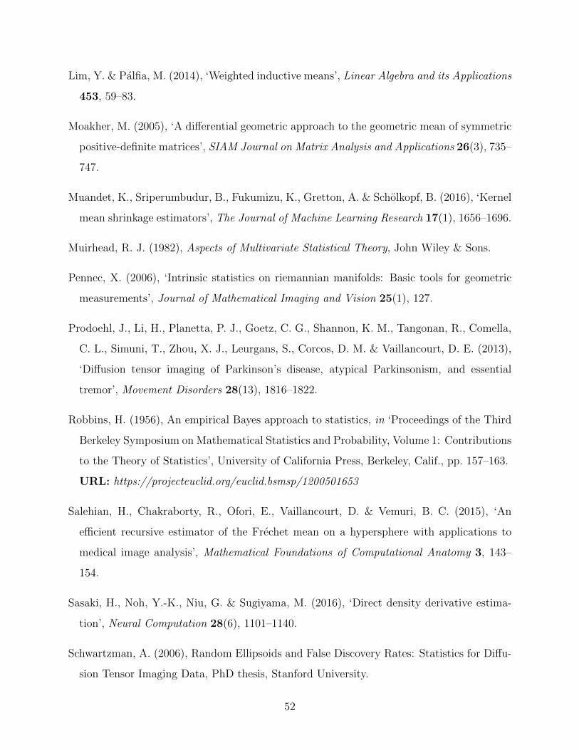
Lim, Y. & Palfia, M. (2014), ‘Weighted inductive means’, Linear Algebra and its Applications

453, 59–83.

Moakher, M. (2005), ‘A differential geometric approach to the geometric mean of symmetric

positive-definite matrices’, SIAM Journal on Matrix Analysis and Applications 26(3), 735–

747.

Muandet, K., Sriperumbudur, B., Fukumizu, K., Gretton, A. & Scholkopf, B. (2016), ‘Kernel

mean shrinkage estimators’, The Journal of Machine Learning Research 17(1), 1656–1696.

Muirhead, R. J. (1982), Aspects of Multivariate Statistical Theory, John Wiley & Sons.

Pennec, X. (2006), ‘Intrinsic statistics on riemannian manifolds: Basic tools for geometric

measurements’, Journal of Mathematical Imaging and Vision 25(1), 127.

Prodoehl, J., Li, H., Planetta, P. J., Goetz, C. G., Shannon, K. M., Tangonan, R., Comella,

C. L., Simuni, T., Zhou, X. J., Leurgans, S., Corcos, D. M. & Vaillancourt, D. E. (2013),

‘Diffusion tensor imaging of Parkinson’s disease, atypical Parkinsonism, and essential

tremor’, Movement Disorders 28(13), 1816–1822.

Robbins, H. (1956), An empirical Bayes approach to statistics, in ‘Proceedings of the Third

Berkeley Symposium on Mathematical Statistics and Probability, Volume 1: Contributions

to the Theory of Statistics’, University of California Press, Berkeley, Calif., pp. 157–163.

URL: https://projecteuclid.org/euclid.bsmsp/1200501653

Salehian, H., Chakraborty, R., Ofori, E., Vaillancourt, D. & Vemuri, B. C. (2015), ‘An

efficient recursive estimator of the Frechet mean on a hypersphere with applications to

medical image analysis’, Mathematical Foundations of Computational Anatomy 3, 143–

154.

Sasaki, H., Noh, Y.-K., Niu, G. & Sugiyama, M. (2016), ‘Direct density derivative estima-

tion’, Neural Computation 28(6), 1101–1140.

Schwartzman, A. (2006), Random Ellipsoids and False Discovery Rates: Statistics for Diffu-

sion Tensor Imaging Data, PhD thesis, Stanford University.

52

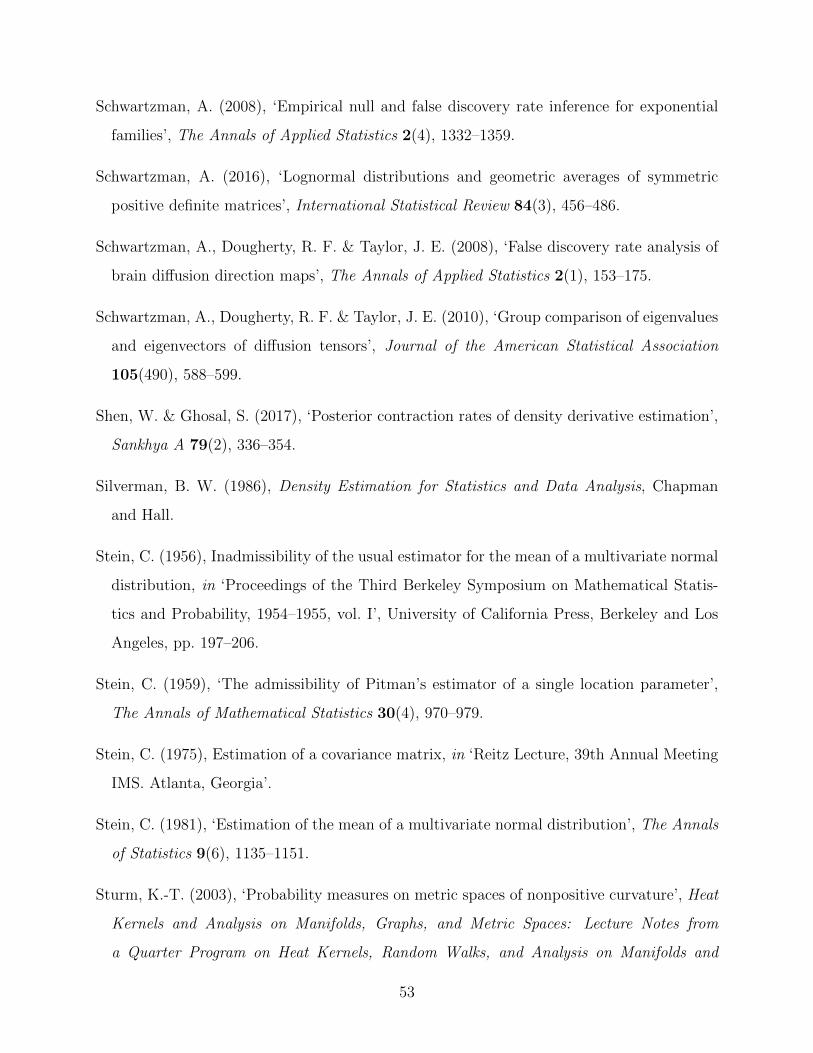
Schwartzman, A. (2008), ‘Empirical null and false discovery rate inference for exponential

families’, The Annals of Applied Statistics 2(4), 1332–1359.

Schwartzman, A. (2016), ‘Lognormal distributions and geometric averages of symmetric

positive definite matrices’, International Statistical Review 84(3), 456–486.

Schwartzman, A., Dougherty, R. F. & Taylor, J. E. (2008), ‘False discovery rate analysis of

brain diffusion direction maps’, The Annals of Applied Statistics 2(1), 153–175.

Schwartzman, A., Dougherty, R. F. & Taylor, J. E. (2010), ‘Group comparison of eigenvalues

and eigenvectors of diffusion tensors’, Journal of the American Statistical Association

105(490), 588–599.

Shen, W. & Ghosal, S. (2017), ‘Posterior contraction rates of density derivative estimation’,

Sankhya A 79(2), 336–354.

Silverman, B. W. (1986), Density Estimation for Statistics and Data Analysis, Chapman

and Hall.

Stein, C. (1956), Inadmissibility of the usual estimator for the mean of a multivariate normal

distribution, in ‘Proceedings of the Third Berkeley Symposium on Mathematical Statis-

tics and Probability, 1954–1955, vol. I’, University of California Press, Berkeley and Los

Angeles, pp. 197–206.

Stein, C. (1959), ‘The admissibility of Pitman’s estimator of a single location parameter’,

The Annals of Mathematical Statistics 30(4), 970–979.

Stein, C. (1975), Estimation of a covariance matrix, in ‘Reitz Lecture, 39th Annual Meeting

IMS. Atlanta, Georgia’.

Stein, C. (1981), ‘Estimation of the mean of a multivariate normal distribution’, The Annals

of Statistics 9(6), 1135–1151.

Sturm, K.-T. (2003), ‘Probability measures on metric spaces of nonpositive curvature’, Heat

Kernels and Analysis on Manifolds, Graphs, and Metric Spaces: Lecture Notes from

a Quarter Program on Heat Kernels, Random Walks, and Analysis on Manifolds and

53

Graphs: April 16-July 13, 2002, Emile Borel Centre of the Henri Poincare Institute,

Paris, France 338, 357–390.

Terras, A. (2016), Harmonic analysis on symmetric spaces—higher rank spaces, positive

definite matrix space and generalizations, Springer.

Tsui, K.-W. (1981), ‘Simultaneous estimation of several Poisson parameters under squared

error loss’, Annals of the Institute of Statistical Mathematics 33(1), 215–223.

Tsui, K.-W. & Press, S. J. (1982), ‘Simultaneous estimation of several Poisson parameters

under k-normalized squared error loss’, The Annals of Statistics 10(1), 93–100.

Tuzel, O., Porikli, F. & Meer, P. (2006), Region covariance: A fast descriptor for detection

and classification, in ‘European Conference on Computer Vision’, Springer, pp. 589–600.

Vaillancourt, D., Spraker, M., Prodoehl, J., Abraham, I., Corcos, D., Zhou, X., Comella, C.

& Little, D. (2009), ‘High-resolution diffusion tensor imaging in the substantia nigra of de

novo Parkinson disease’, Neurology 72(16), 1378–1384.

Wang, Z. & Vemuri, B. C. (2004), Tensor field segmentation using region based active contour

model, in ‘European Conference on Computer Vision’, Springer, pp. 304–315.

Xie, X., Kou, S. C. & Brown, L. D. (2012), ‘SURE estimates for a heteroscedastic hierarchical

model’, Journal of the American Statistical Association 107(500), 1465–1479.

Xie, X., Kou, S. C. & Brown, L. D. (2016), ‘Optimal shrinkage estimation of mean parameters

in family of distributions with quadratic variance’, The Annals of Statistics 44(2), 564–597.

Yang, C.-H. & Vemuri, B. C. (2019), Shrinkage estimation on the manifold of symmetric

positive-definite matrices with applications to neuroimaging, in ‘International Conference

on Information Processing in Medical Imaging’, Springer, pp. 566–578.

Zhou, D., Dryden, I. L., Koloydenko, A. & Li, B. (2008), A Bayesian method with repa-

rameterization for diffusion tensor imaging, in ‘Medical Imaging 2008: Image Processing’,

Vol. 6914, International Society for Optics and Photonics, p. 69142J.

54

An Empirical Bayes Approach to Shrinkage Estimation ... - arXiv

Documents

Transcript of An Empirical Bayes Approach to Shrinkage Estimation ... - arXiv