Stat Comput (2007) 17:163–177DOI 10.1007/s11222-006-9012-9

Maximum likelihood from spatial random effects models via thestochastic approximation expectation maximization algorithmHongtu Zhu · Minggao Gu · Bradley Peterson

Received: March 2004 / Accepted: August 2006 / Published online: 27 January 2007C© Springer Science + Business Media, LLC 2007

Abstract We introduce a class of spatial random effectsmodels that have Markov random fields (MRF) as latentprocesses. Calculating the maximum likelihood estimatesof unknown parameters in SREs is extremely difficult,because the normalizing factors of MRFs and additionalintegrations from unobserved random effects are computa-tionally prohibitive. We propose a stochastic approximationexpectation-maximization (SAEM) algorithm to maximizethe likelihood functions of spatial random effects models.The SAEM algorithm integrates recent improvementsin stochastic approximation algorithms; it also includescomponents of the Newton-Raphson algorithm and theexpectation-maximization (EM) gradient algorithm. Theconvergence of the SAEM algorithm is guaranteed undersome mild conditions. We apply the SAEM algorithmto three examples that are representative of real-worldapplications: a state space model, a noisy Ising model, andsegmenting magnetic resonance images (MRI) of the humanbrain. The SAEM algorithm gives satisfactory results infinding the maximum likelihood estimate of spatial randomeffects models in each of these instances.

H. Zhu (�)Department of Biostatistics and Biomedical Research ImagingCenter, University of North Carolina at Chapel Hill, Chapel Hill,NC 27599-7420, USAe-mail: htzhu@email.unc.edu

H. Zhu . B. PetersonDepartment of Psychiatry, Columbia University and New YorkState Psychiatric Institute, 1051 Riverside Drive, Unit 74, NewYork, New York 10032, USA

M. GuDepartment of Statistics, The Chinese University of Hong Kong,Shatin, N.T., Hong Kong, P.R. China

Keywords Expectation maximization . Markov chainMonte Carlo . Markov random fields . Spatial randomeffects models . Stochastic approximation

1 Introduction

Spatial random effects models, also called hidden Markovmodels, represent a natural extension of Markov randomfields (Besag, 1986, 1974). Spatial random effects modelsare very useful for accommodating overdispersion amongoutcomes (Zeger et al., 1988) and for interpolating orsmoothing spatial and image data (Diggle et al., 1998).Special classes of spatial random effects models include:generalized linear mixed models, such as those used inbiomedical studies (Breslow and Clayton, 1993; Lee andNelder, 1996); spatial generalized linear mixed models(SGLMM), as used in geostatistics (Christensen andWaagepetersen, 2002; Zhang, 2002); and noisy GaussianMarkov random fields (GMRF), as applied for image seg-mentation and restoration in image analysis (Saquib et al.,1998; Rajapakse et al., 1997; Marroquin et al., 2003).

Because of the utility of spatial random effects models,developing procedures for estimating the maximum likeli-hood estimate of spatial random effects models has been anissue of central importance (Marroquin et al., 2003; Qian andTitterington, 1991). Spatial random effects models involvelatent MRFs, whose normalizing factors are notorious fortheir computational complexity. This complexity makescalculating the maximum likelihood estimate of MRFs,and therefore the maximum likelihood estimate of spatialrandom effects models, prohibitively difficult. A secondissue is the additional integrations found in spatial randomeffects models. Most existing procedures for approximatingthe maximum likelihood estimate of MRFs include the

Springer

164 Stat Comput (2007) 17:163–177

Monte Carlo likelihood inference (Geyer and Thompson,1992), Monte Carlo Newton-Raphson sampling (Penttinen,1984), numerical approximations (Pettitt et al., 2003), andthe stochastic approximation algorithm (Younes, 1989;Moyeed and Baddeley, 1991; Gu and Zhu, 2001). However,these algorithms cannot be applied directly to calculatingthe maximum likelihood estimate of spatial random effectsmodels because they do not account for the presence inspatial random effects models of additional integrationsfrom unobserved random effects (Qian and Titterinton,1991). Ryden (1997) proposed a stochastic approximationalgorithm for recursive estimation of hidden Markov models,Delyon et al. (1999) proposed a stochastic approximationEM algorithm for curved exponential families with randomeffects, and Zhang (2002) proposed a Monte Carlo EMalgorithm for computing the maximum likelihood estimateof spatial generalized linear mixed models. However, nei-ther of these models contains any normalizing factors thatare intractable; the estimation algorithms for these modelstherefore cannot be applied to spatial random effects models.

We propose an SAEM algorithm for computing the max-imum likelihood estimate of spatial random effects mod-els, and we give a proof of its convergence under someconditions. Examples of a state space model, a noisy Isingmodel, and image segmentation in MRI illustrate the ef-fective performance of our SAEM algorithm in calculatingthe maximum likelihood estimate of spatial random effectsmodels.

2 Spatial random effect models

2.1 Definition of spatial random effects models

We consider a data set that is composed of a response y j (si )and covariate vector x j (si ) for j = 1, . . . , mi at a site si ∈ Sfor i = 1, . . . , n, where S = {si : i = 1, . . . , n} is a knowndiscrete index set. For instance, in image processing, si rep-resents the location of a particular voxel/pixel. Furthermore,we assume that there is an unobserved d × 1 random effectvector b(si ) for each y(si ) = (y1(si ), . . . , ymi (si ))T . Spatialrandom effects models are defined as follows.

(i) Conditional on b = (b(s1), . . . , b(sn))T , the componentsof Y = ( y(s1), . . . , y(sn))T are mutually independent,and the conditional density of y(si ) given b is a memberof the exponential family (McCullagh and Nelder, 1989)given by

p( y(si )|b; α, β)=mi∏

j=1

exp{φ j (si )[y j (si )θ j (si )−a(θ j (si ))]

+c(y j (si ), φ j (si ))}, (1)

where φ j (si ) = φ j (α, b(si )), α is an unknown q1 × 1 pa-rameter vector, and a(·) and c(·) are known continuouslydifferentiable functions. For a known link function h1(·),

µ j (si ) = E[y j (si )|b] = h1(x j (si )T β, b(si )), (2)

where β is a q2 × 1 parameter vector.(ii) The joint distribution of random effects b has the Gibbs

form:

p(b|τ ) = exp{−U (b)T h2(τ ) − log C(τ )}, (3)

where h2(·) is a known function, τ is a q3 × 1 vectorcharacterizing the granularity of MRF, and U (b)T h2(τ )is a potential (or energy) function, which exhibits theinteraction between random effects (Besag, 1974). Inaddition, the normalizing factor C(τ ), called a partitionfunction, has the form

C(τ ) =∫

b∈Bexp{−U (b)T h2(τ )}m(db), (4)

where B is the minimal sample space of b and m(db) iseither the Dirac’s delta measure or db.

The likelihood function of observed data Y = yo for anspatial random effects model is given by

L(ξ ; yo) =∫

Bexp{−U (b)T h2(τ )

− log C(τ )}n∏

i=1

p( y(si )|b; α, β)m(db), (5)

where ξ T = (αT , βT , τ T ) is a q × 1 (q = q1 + q2 + q3) vec-tor of unknown parameters. Because the integration aboveis usually of very high dimension and/or C(τ ) is difficult toobtain analytically, evaluating L(ξ ; yo) is computationallyprohibitive.

2.2 Examples of spatial random effects models

We examine three examples of spatial random effects mod-els:

Example 1 (Generalized linear mixed models). General-ized linear mixed models usually assume that randomeffects b(si ) are normally distributed with zero mean andcovariance matrix �b and b(si ) and b(si ′) are independentof each other for si �= si ′ . See, for example, Breslowand Clayton (1993), Aitkin (1996), and Zhu and Lee(2002), among many others. For generalized linear mixedmodels, si ∈ S can represent either a subject or a clusterin a longitudinal study or a family in a familial study.

Springer

Stat Comput (2007) 17:163–177 165

In particular, U (b)T h2(τ ) = 0.5∑n

i=1 b(si )T �−1b b(si )

and log C(τ ) = 0.5n log |�b| + 0.5nd log(2π ), where τ

contains all unknown parameters in �b.

Example 2 (State space models). State space models repre-sent further extensions of generalized linear mixed models byconsidering time series dependence among random effectsb(si ) (Chan and Ledolter, 1995; Durbin and Koopman, 1997,2000). In this case, each si denotes a time point such thats1 < s2 < · · · < sn . For example, in the time series of countdata considered in Section 4.1, y(si ) follows the Poisson dis-tribution with mean µ(si ) = exp(x(si )T β + b(si )). Assumethat b(s1) is given and {b(si )} is a stationary Gaussian AR(1)process, that is, b(si ) = ρb(si−1) + εi , where {εi } is identi-cally and independently distributed as N (0, σ 2

ε ). Thus, τ =(ρ, σ 2

ε )T , U (b)T h2(τ ) = ∑n−1i=1 [b(si+1) − ρb(si )]2/(2σ 2

ε ),and log C(τ ) = [(n − 1) /2] log(σ 2

ε ).

Example 3 (Spatial random effects models for image seg-mentation). Image segmentation is among the several im-portant image processes that have been modeled by usingspatial random effects models since the seminal papers byGeman and Geman (1984) and Besag (1974). See, for ex-ample, Winkler (1995), Li (2001), Rajapakse et al. (1997),and Marroquin et al. (2003), among many others. For im-age segmentation, si ∈ S denotes either a pixel site or a linesite in a pixelated image, Y denotes the observed image,and each b(si ) in b denotes the true identity at the voxel si .The purpose of image segmentation is to classify Y into Mnonoverlapping regions {R1, . . . , RM}.

A simple example of spatial random effects modelsfor image segmentation (Qian and Titterington, 1991;Besag, 1986; Derin and Elliott, 1987) assumes thatYi |b(si ) ∼ N (µ(b(si )), σ 2) for i = 1, . . . , n, and p(b|τ ) =exp{τ ∑si ∼s j

δ(b(si ), b(s j )) − log C(τ )}, where b(si ) takesvalue from 1 to M , the summation is over nearest-neighborpairs si ∼ s j , and δ(x, z) is the Kronecker function equalingto 1 when x = z and 0 otherwise. The potential func-tion U (b) = −∑si ∼s j

δ(b(si ), b(s j )) and the normalizingfactor C(τ ) = ∑

b exp(−U (b)τ ), which involves Mn

terms.We consider a generalization of a spatial random effects

model for image segmentation of MRI from Zhang et al.(2001) as follows. The observation y(si ) at a particular voxelsi can be modeled as

y(si ) = x0(si )T β0 +

M∑

k=1

[x1(si )T β(k) + εk(si )]δ(b(si ), k),

(6)

where x0(si ) and x1(si ) are, respectively, covariate vectorscharacterizing common and individual features at the

voxel si , b(si ) ∈ {1, . . . , M}, εk(si ) ∼ N (0, eσk ), and βk

is the parameter vector associated with the class Rk .We further assume that the joint distribution of the la-bel fields b is given by p(b|τ ) = exp{∑n

i=1 τ1(b(si )) +∑si ∼s j

τ2δ(b(si ), b(s j )) − log C(τ )}, where τ1(b(si )) maydepend on the value of b(si ) and τ1(1) is set to zero to avoidredundancy, τ2 controls the granularity of MRF, and τ =(τ1(2), . . . , τ1(M), τ2)T . The potential function U (b)T τ =(−∑n

i=1 δ(b(si ), 2), . . . ,−∑ni=1 δ(b(si ), M),−∑

si ∼s jδ(b

(si ), b(s j ))τ and the normalizing factor C(τ ) is ob-tained by summing all possible configurations b,C(τ ) = ∑

b exp(−U (b)T τ ). If τ2 = 0, then log C(τ ) =n log[1 +∑M

k=2 exp(τ1(k))] and the above spatial randomeffects model reduces to a mixture linear regression model(Zhang et al., 2001; Zhu and Zhang, 2004).

3 SAEM algorithm

Under the spatial random effects model specified by (1), (2),and (3), the maximum likelihood estimate of ξ , denoted byξ = (α, β, τ ), is defined by

L(ξ ; yo) = maxξ

L(ξ ; yo). (7)

Because L(ξ ; yo) in (5) is computationally intractable, it isinfeasible to maximize the likelihood function of observeddata directly. Instead, we consider the first-order and second-order partial derivatives of the log-likelihood function inorder to use gradient-type algorithms, such as the Newton-Raphson and Gauss-Newton algorithms (Ortega, 1990).

3.1 First-order and second-order derivatives of thelog-likelihood function

The first-order and second-order derivatives of thelog-likelihood functions can be derived by using thelog-likelihood functions of complete data, denoted bylc(ξ ; b, yo), which is given by

n∑

i=1

mi∑

j=1

{φ j (si )[y j (si )θ j (si ) − a(θ j (si ))] + c(y j (si ), φ j (si ))}

−U (b)T h2(τ ) − log C(τ ). (8)

From the missing information principle, the first-orderderivative of L(ξ ; yo), called the score function, can be writ-ten as

sξ (ξ ; yo) = ∂ξ log L(ξ ; yo) = E[Sξ (ξ ; b)| yo, ξ ], (9)

where Sξ (ξ ; b) = ∂ξ lc(ξ ; b, yo) and E[·| yo, ξ ] denotes thatthe expectation is taken with respect to the conditional

Springer

166 Stat Comput (2007) 17:163–177

distribution p(b|Y = yo, ξ ). In addition, we use ∂ and ∂2

to denote the first-order and second-order derivatives withrespect to a parameter vector, say, ∂ξ a(ξ ) = ∂a(ξ )/∂ξ and∂2ξ a(ξ ) = ∂2a(ξ )/∂ξ∂ξ T . To calculate the second-order

derivative of the log-likelihood function, we apply Louis’s(1982) formula to obtain

− ∂2ξ log L(ξ ; yo) = E[Iξξ (ξ ; b) − Sξ (ξ ; b)⊗2| yo, ξ ]

+ sξ (ξ ; yo)⊗2, (10)

where for vector a, a⊗2 = aaT and Iξξ (ξ ; b) = −∂2ξ lc

(ξ ; b, yo) denotes the information matrix for complete data.We obtain explicit forms of the first-order and

second-order derivatives of lc(ξ ; b, yo). By differentiatinglc(ξ ; b, yo) with respect to ξ , we obtain

Sα(ξ ; b) =n∑

i=1

mi∑

j=1

∂αφ j (si )[y j (si )θ j (si ) − a(θ j (si ))

+ ∂φ j c(y j (si ), φ j (si ))],

Sβ(ξ ; b) =n∑

i=1

mi∑

j=1

φ j (si )e j (si )∂βθ j (si ), and (11)

Sτ (ξ ; b) = −U (b)T ∂τ h2(τ ) − ∂τ log C(τ ),

where e j (si ) = y j (si ) − µ j (si ). With some algebraic manip-ulation, we obtain

Iββ(ξ ; b)=n∑

i=1

mi∑

j=1

{φ j (si )∂βθ j (si )

T[∂2θ j

a(θ j (si ))]∂βθ j (si )

−φ j (si )e j (si )∂2βθ j (si )

},

Iβα(ξ ; b)=−n∑

i=1

mi∑

j=1

∂αφ j (si )e j (si )∂βθ j (si ),

Iττ (ξ ; b)=∂2τ [U (b)T h2(τ )] + ∂2

τ log C(τ ), (12)

Iαα(ξ ; b)=−n∑

i=1

mi∑

j=1

∂2αφ j (si ){[y j (si )θ j (si ) − a(θ j (si ))]

+ ∂φ j c(y j (si ), φ j (si ))}

−n∑

i=1

mi∑

j=1

∂αφ j (si )T ∂2

φ jc(y j (si ), φ j (si ))∂αφ j (si ),

Iβτ (ξ ; b)=0, and Iατ (ξ ; b) = 0.

Because Iβα(ξ ; b) is close to zero at the maximum likelihoodestimate, we set Iβα(ξ ; b) = 0 in the SAEM algorithm, whichleads to a stable algorithm when the initial parameters arefar from the maximum likelihood estimate.

To calculate the score function in (9) and the informationmatrix in (10), we need to calculate ∂τ log C(τ ) and

∂2τ log C(τ ). Following Gelman and Meng (1998), we

have

∂τ log C(τ ) = −Eτ

[U (b)T ∂τ h2(τ )

]and

∂2τ log C(τ ) = −Eτ [J (τ ; b)] − {∂τ log C(τ )}⊗2 , (13)

where J (τ ; b) = ∂2τ [U (b)T h2(τ )] − [U (b)T ∂τ h2(τ )]⊗2 and

Eτ is taken with respect to the MRF (3). One way to calculate∂τ log C(τ ) and ∂2

τ log C(τ ) is to use numerical integrationby using Eq. (13); however, the numerical integration is ac-curate only in a few special cases. Another way is to resortto Monte Carlo methods (Liu, 2001; Møller, 1999; Robertsand Casella, 1999; Gu and Zhu, 2001). If we can simulate{bk : k = 1, . . . , Nk} from the MRF (3), then we can use Eq.(13) to obtain the Monte Carlo approximation of ∂τ log C(τ )and ∂2

τ log C(τ ). Moreover, Eq. (13) is also the basis forthe method of path sampling for estimating C(τ ) at any τ

(Gelman and Meng, 1998; Huang and Ogata, 2001; Pettittet al., 2003). Explicitly, the path sampling method is basedon the following formula:

log C(τ ∗∗) − log C(τ ∗) =∫ τ ∗∗

τ ∗∂τ log C(τ )dτ

= −∫ τ ∗∗

τ ∗Eτ [U (b)T ∂τ h2(τ )]dτ.

Thus, the Monte Carlo methods can be used to approximateEτ [U (b)T ∂τ h2(τ )] at each τ and then estimate log[C(τ ∗∗)] −log[C(τ ∗)].

We use Eqs. (11), (12), and (13) to calculate thefirst-order and second-order derivatives of the likelihoodfunctions of observed data. The score function can bewritten as (Sα(ξ ; b)T , Sβ (ξ ; b)T , [Sτ,1 − Sτ,2]T )T , whereSτ,2 = ∂τ log C(τ ) and Sτ,1 = −Eξ [U (b)T ∂τ h2(τ )| yo, ξ ].We define

I1(ξ ; b) =

⎛

⎜⎝Iαα(ξ ; b) 0 0

0 Iββ(ξ ; b) 0

0 0 ∂2τ [U (b)T h2(τ )]

⎞

⎟⎠ and

I2(ξ ; b) = −

⎛

⎜⎝Sα(ξ ; b)

Sβ(ξ ; b)

−U (b)T ∂τ h2(τ )

⎞

⎟⎠

⊗2

.

The information matrix −∂2ξ log L(ξ ; yo) is given by

Eξ [I1(ξ ; b)| yo, ξ ] +(

0 0

0 −Eτ [J (τ ; b)] − (Sτ,2)⊗2

)

+Eξ [I2(ξ ; b)| yo, ξ ]

+(

0 0

0 −(Sτ,2)⊗2+Sτ,1STτ,2 + Sτ,2ST

τ,1,

)+ sξ (ξ ; yo)⊗2.

(14)

Springer

Stat Comput (2007) 17:163–177 167

3.2 Basic steps of the SAEM algorithm

At the k-th iteration, ξ k is the current estimate of ξ ; hk ,the current estimate of sξ (ξ ; yo); Sk

τ,1 is the current estimateof Eξ [−U (b)T ∂τ h2(τ )| yo, ξ ]; Sk

τ,2, the current estimate of−∂τ log C(τ ); �k

1, the current estimate of Eξ [I1(ξ ; b)| yo, ξ ];�k

2, the current estimate of Eξ [I2(ξ ; b)| yo, ξ ]; and �k3, the

current estimate of Eτ [J (τ ; b)]. We assume that �τ (·, ·) isthe Markov transition probability of the Metropolis-Hasting(MH) algorithm used to simulate from the MRF (3), and� yo,ξ

(·, ·) is the transition probability of the MH algorithmused to simulate from the conditional distribution of b givenyo and ξ .

Step 1. At the kth iteration, set bk,0 = bk−1,Nk−1 andby,k,0 = by,k−1,Nk−1 . Generate bk = (bk,1, . . . , bk,Nk ) andby,k = (by,k,1, . . . , by,k,Nk ) from the transition probabilities�τ k−1 (bk,i−1, ·) and � yo,ξ

k−1 (by,k,i−1, ·), respectively.

Step 2. Update the seven estimates as follows:⎧⎪⎪⎪⎪⎪⎪⎪⎪⎪⎪⎪⎪⎨

⎪⎪⎪⎪⎪⎪⎪⎪⎪⎪⎪⎪⎩

ξ k = ξ k−1 + γk[�(t)k]−1 H (ξ k−1; bk, by,k),

hk = hk−1 + γk(H (ξ k−1; bk, by,k) − hk−1),

�k1 = �k−1

1 + γk(I 1(ξ k−1; by,k) − �k−1

1

),

�k2 = �k−1

2 + γk(I 2(ξ k−1; by,k) − �k−1

2

),

�k3 = �k−1

3 + γk(J (τ k−1; bk) − �k−1

3

),

Skτ,1 = Sk−1

τ,1 + γk(−U (by,k)T ∂τ h2(τ k−1) − Sk−1

τ,1

),

Skτ,2 = Sk−1

τ,2 + γk(U (bk)∂τ h2(τ k−1) − Sk−1

τ,2

),

(15)

where t ∈ [0, 1], J (τ ; bk) = N−1k

∑Nki=1 J (τ ; bk,i ),

I 1(ξ ; by,k) =Nk∑

i=1

I1(ξ ; by,k,i )/Nk,

I 2(ξ ; by,k) =Nk∑

i=1

I2(ξ ; by,k,i )/Nk,

U (by,k)T ∂τ h2(τ ) = Nk−1

Nk∑

i=1

U (by,k,i )T ∂τ h2(τ ),

U (bk)T ∂τ h2(τ ) = Nk−1

Nk∑

i=1

U (bk,i )T ∂τ h2(τ ),

H (ξ ; bk, by,k) =(

1

Nk

Nk∑

i=1

Sα(ξ ; by,k,i )T ,

1

Nk

Nk∑

i=1

Sβ(ξ ; by,k,i )T ,

[−U (by,k) + U (bk)]T ∂τ h2(τ )

)T

.

In addition, �(t)k is a current estimate of E[Iξξ (ξ ; b)−t Sξ (ξ ; b)⊗2| yo, ξ ] + sξ (ξ ; yo)⊗2 given by

�k1 + [hk]⊗2 + t�k

2

+(

0 0

0 −�k3 − (1 + t)(Sk

τ,2)⊗2 + t Skτ,1SkT

τ,2 + t Skτ,2SkT

τ,1,

).

(16)

Finally, the gain constants sequence {γk} satisfies the follow-ing conditions:

0 ≤ γk ≤ 1 for all k,

∞∑

k=1

γk = ∞ and∞∑

k=1

γ 2k < ∞.

(17)

An important feature of the SAEM algorithm is that ituses a gain constants sequence {γk} to handle the noise inapproximating ∂ξ log L(ξ ; yo) and ∂2

ξ log L(ξ ; yo) in Step 2(Robbins and Monro, 1951; Lai, 2003). In principle, thechoice of Nk should not affect the convergence of thestochastic approximation algorithm, but a good choice ofNk can improve the performance of the SAEM algorithm.At the end of the SAEM algorithm, �k(1), �k(0), and�k(0) − �k(1) can be used to estimate the observed-data,completed-data and missing-data information matrix,respectively (Louis, 1982). For some models, �k(1) may notbe positive definite, but the corresponding �k(0) is positivedefinite (Lange, 1995). Based on three examples in Section4, we suggest using �k(0) in the SAEM algorithm.

3.3 Two stages of the SAEM algorithm

Following Gu and Zhu (2001), our procedure to find ξ de-fined by (7) is composed of two stages. The main idea of thetwo stages is based on the observation that, if the startingpoint is not in the neighborhood of the maximum likelihoodestimate, then the SAEM algorithm will usually convergeslowly. In Stage I, we use a large gain constants sequenceso that the parameter will move quickly into the vicinityof the maximum likelihood estimate. In Stage II, we use asmall gain constants sequence to stabilize the algorithm inthe neighborhood of the maximum likelihood estimate andan off-line averaging method to achieve the optimal conver-gence rate.

The main procedure is implemented as follows.

Stage I. Iterate Steps 1 and 2 with i = 1, . . . , K1 and the gainconstants are defined by

γi = γ1i = b1/(i a1 + b1 − 1), i = 1, . . . , K1,

Springer

168 Stat Comput (2007) 17:163–177

where K1 ≥ K0 is determined by

K1 = inf{

K ≥ K0 : �(1)i

=∥∥∥∥∥∥

K∑

i=K−K0+1

Sign(ξ i − ξ i−1)/K0

∥∥∥∥∥∥≤ η1

⎫⎬

⎭ . (18)

Function Sign(z) is a vector of 1, 0, or −1 accordingto whether each component of z is positive, zero, ornegative, respectively. Integers b1 and K0, real num-ber a1 ∈ (0, 1), and η1 are pre-assigned constants. Wechoose a1 to be close to 0.5 and b1 to be relativelylarge (e.g., a1 = 0.3 and b1 = 5) to obtain large gainconstants. Also, we choose a relatively small value ofη1 and K0 (e.g., η1 = 0.1 and K0 = 100) to ensure thatthe estimates ξ i s start to move around a certain point,possibly the maximum likelihood estimate.

Stage II. Take the seven estimates in the last iteration of StageI as their initial values in Stage II. We iterate Steps 1 and2 with i = 1, . . . , K2 and the gain constants are definedby

γi = γ2i = b2/(i a2 + b2 − 1), i = 1, . . . , K2,

where integer b2 and a2 ∈ (1/2, 1] are preassigned. Wechoose a2 close to 1 and a small integer for b2 (e.g.,a2 = 0.8, b2 = 2) to obtain small gain constants andto stabilize the algorithm. We use an off-line averag-ing procedure at the same time. We set the initial es-

timates as ξ 0 = ξ K1 , h0 = hK1 , �

01 = �

K11 , �

02 = �

K12 ,

�03 = �

K13 , S0

τ,1 = SK1τ,1, S0

τ,2 = SK1τ,2, and �

0(t) = �K1 (t),

and then update eight estimates as follows:

ξ i = ξ i−1 + (ξ i − ξ i−1)/ i,

hi = h

i−1 + (hi − hi−1

)/ i,

Siτ,m ′ = Si−1

τ,m ′ + (Siτ,m ′ − Si

τ,m ′ )/ i,

�im = �

i−1m + (�i

m − �i−1m )/ i, and

�i(t) = �

i−1(t) + [�i (t) − �

i−1(t)]/ i, (19)

where m = 1, 2, 3 and m ′ = 1, 2. Theoretically, thisoff-line averaging procedure automatically leads to anoptimal convergence without estimating the informa-tion matrix (Polyak, 1990; Polyak and Juditski, 1992).The stopping rule of Stage II is defined by

K2 = inf{i : �

(2)i ≤ η2

}, (20)

where �(2)i = h

iT[�

i(1)]−1 h

i + tr{[�i(1)]−1�}/ i, in

which � denotes an estimate of �, the covariance

matrix of Monte Carlo error. A rough estimate of �

can be achieved by taking the sample covariance ofH (ξ k−1; bk, by,k). The value of η2 is usually taken tobe around 0.002 to ensure small values of sξ (ξ ; yo)as the convergence criterion of the SAEM algorithm(Gu and Zhu, 2001). At the K2-th iteration, we use theoff-line average (ξ K2 , �

K2 (1)) as our final estimate of(ξ ,−∂2

ξ log L(ξ ; yo)).

3.4 Convergence of the SAEM algorithm

We first establish the convergence of an algorithm, which isan approximation to the SAEM algorithm. Note that the max-imum likelihood estimate ξ , defined by (7), can be obtainedas a solution to

sξ (ξ , yo) = H (ξ ) = E[Sξ (ξ ; b)| yo, ξ ] = 0. (21)

Without loss of generality, we assume that ∂τ log C(τ )and ∂2

τ log C(τ ) can be evaluated analytically so that wecan omit the step of sampling from the MRF (3). Wealso define Gt (ξ, b) = Iξξ (ξ, b) − t Sξ (ξ ; b)⊗2 and Gt (ξ ) =E[Gt (ξ, b)| yo, ξ ]. In principle, Step 2 of the SAEM algo-rithm is equivalent to

{ξ k = ξ k−1 + γk[�k(t)]−1 H (ξ k−1; by,k),

�k(t) = �k−1(t) + γk[Gt (ξ k, by,k) − �k−1(t)],(22)

where H (ξ k−1; by,k) = ∑Nkl=1 Sξ (ξ ; by,k,l)/Nk and Gt (ξ,

by,k) = ∑Nkl=1 Gt (ξ ; by,k,l )/Nk . The basic iteration in (22)

can be further viewed as an approximation to

⎧⎨

⎩ξ

k = ξk−1 + γk[�

k(t)]−1 H (ξ

k−1),

�k(t) = �

k−1(t) + γk[Gt (ξ

k−1) − �

k−1(t)],

(23)

where we use notation ξk

and �k(t) to represent the estimates

generated from (23). The algorithm in (22) can be convergentonly if (23) is convergent.

We establish the geometric convergence of (23) in Theo-rem 1. A detailed proof is given in Zhu and Gu (2005). Theproof follows the general arguments for showing the conver-gence of the Newton-Raphson algorithm (Stoer and Bulisch,1980). Let ‖ · ‖ be a norm on Rq , the norm of a q × q ma-trix A is defined as ‖A‖ = maxx:‖x‖=1 ‖Ax‖, where x =(x1, . . . , xq )T is a vector. We assume that functions H (ξ )and Gt (ξ ) are both differentiable on a convex set C0 ⊂ Rq .

Lemma 1. Assume that ξ ∈ C0 is a root of H (ξ ) and {ξ :‖ξ − ξ‖ ≤ ca} ⊂ C0 for some ca. Suppose that the sequence

{ξ k, k > 0} is defined by (23) with initial value ξ

0 ∈ C0.Assume that

Springer

Stat Comput (2007) 17:163–177 169

(a) ‖∂ξ H (ξ )−∂ξ H (ξ ′)‖ ≤ cη‖ξ−ξ ′‖ for every ξ, ξ ′ ∈ C0;

(b) ‖ξ 0 − ξ‖ ≤ ca;

(c) ‖[�k(t)]−1‖ ≤ cb, for k = 0, 1, . . . ;

(d) ‖Iq − B‖ ≤ 1 − λ, where Iq is a q × q identity matrix,

1 > λ ≥ 0 and B = −[�k(t)]−1∂ξ H (ξ );

(e) δ = λ − cacbcη > 0.

Then for each k ≥ 0,

‖ξ k − ξ‖ ≤ exp{−δTk}‖ξ 0 − ξ‖, (24)

where T0 = 0 and Tk = ∑ki=1 γi .

Theorem 1 (Geometric convergence of the algorithm (23)).

Suppose that ξ0 ∈ C0 and �

0(t) is a positive definite matrix

and that {γk, k ≥ 1} is a sequence of positive numbers such

that γk ≤ 1. For sequence {ξ k,�

k(t), k ≥ 0} as defined

in (23) with initial values ξ0

and �0(t), assume that

Assumption (a) to (c) in Lemma 1 are valid. Further assumethat

(f) ‖Gt (ξ ) − Gt (ξ ′)‖ ≤ cd‖ξ − ξ ′‖ for every ξ, ξ ′ ∈ C0;(g) ‖Gt (ξ )−1‖ ≤ cb for all ξ ∈ C0;(h) ‖G−1

t (ξ )[Gt (ξ ) + ∂ξ H (ξ )]‖ ≤ 1 − λ for all ξ ∈ C0,where 1 ≥ λ > 0;

(i) ‖Gt (ξ ) − �0(t)‖ ≤ cacd ;

(j) δ′ = 1 − cacbcd + (1 − λ)(1 − cacbcd )−1 > 0.Then for each k ≥ 0,

‖ξ k − ξ‖ ≤ exp{−δ′Tk}‖ξ 0 − ξ‖, (25)

and if Tk ≥ 3, then

‖�k(t) − Gt (ξ )‖ ≤ exp{−δ′Tk/2}[‖Gt (ξ )

−�0(t)‖ + 2cd‖ξ − ξ

0‖]. (26)

Theorem 1 generalizes Ostrowski’s Theorem to establisha geometric convergence of algorithm (23) (Ortega, 1990).If γk = 1 for all k, then algorithm (23) reduces to a stan-dard iterative method for solving sξ (ξ , y0) = 0. Under al-most the same conditions as in Theorem 1, Ostrowski’s The-orem states that ξ is a point of attraction. That is, there is an

open neighborhood C0 of ξ such that whenever ξ0 ∈ C0, the

iterations in algorithm (23) are well defined and the sequence

ξk

converges to ξ (Ortega, 1990, p. 144–145). Theorem 1 foralgorithm (23) is more general because {γk : k ≥ 1} is a se-quence of positive numbers satisfying γk ≤ 1.

Next, we provide a convergence theorem of the algo-rithm (22). When the functions H (ξ ) and Gt (ξ ) cannot beexplicitly calculated, we may substitute them with MonteCarlo estimates, which results to the algorithm given by

(22). We follow the ordinary differential equation (ODE)method (see Chapter 2 of Benveniste et al., 1990). Sup-pose that we have a vector function ξ (v) and a matrixfunction �(v), v ≥ 0, satisfying the ordinary differentialequations

dξ (v)

dv= �(v)−1 H (ξ (v)),

d�(v)

dv= Gt (ξ (v)) − �(v),

(27)

with the initial condition ξ (0) = ξ 0 and �(0) = �0. It isshown in Benveniste et al. (1990) that the function ξ (v) isclosely related to the estimates ξ k produced by (22) with thesame initial vector. It is easy to see that (ξ , Gt (ξ )) is a stabilitypoint of the above differential equation and all eigenvaluesof Gt (ξ )−1∂ξ H (ξ ) have negative real parts. A set D is calleda domain of attraction of a stability point (ξ , Gt (ξ )) if thesolution of (27) with (ξ (0),�(0)) ∈ D remains indefinitelyin D and converges to (ξ , Gt (ξ )). Theorem 1 guarantees theexistence of such a set D.

Assume that the transition probability �(·, ·|ξ ) satisfiesthe conditions (C.3)−(C.6) given in Gu and Kong (1998). Weassume that (C.7) holds for the functions Sξ (ξ ; b), Sξ (ξ ; b)⊗2,and Iξξ (ξ ; b). Under these conditions, the results consideredin Gu and Kong (1998) hold in our case. Therefore, we havethe following theorem.

Theorem 2. Assume that the conditions (C.1)–(C.7) in Guand Kong (1998) are valid. If {(ξ k,�k(t)), k ≥ 1} from theSAEM algorithm (22) is a bounded sequence and visits in-finitely often a compact subset of the domain of attractionof the stability point (ξ , Gt (ξ )) of the differential Eq. (27)almost surely, then

ξ k → ξ and �k(t) → Gt (ξ ) almost surely.

4 Examples

We used one simulation study and two real datasets to illus-trate the performance of the SAEM algorithm. All compu-tations were done in C on a SUN HPC4500 workstation. Inall examples, the convergence criterion in (18) and (20) wasused in Stages I and II, respectively, and (K0, η1, η2) was setat (100, 0.1, 0.001).

4.1 State space model

State space models have received much consideration fromboth classical and Bayesian perspectives; see Durbin andKoopman (1997, 2000) and references therein. One special

Springer

170 Stat Comput (2007) 17:163–177

state space model considered in Durbin and Koopman(2000) assumes that the latent process {b(s)} satisfiesb(s) = u(s)b(s − 1) + r(s)ε(s), where ε(s) ∼ p(·|τ ) andboth u(s) and r(s) may depend on unknown parameters.Given {b(s)}, the observations y(s) are conditionallyindependent and follow the distribution (1) with µ(s) =x(s)T β + b(s). Although the maximum likelihood estimatehas good theoretical properties (Ledet and Petersen, 1999),the log-likelihood function of this model does not have asimple closed form and so the maximum likelihood estimateis usually intractable (Chan and Ledolter, 1995; Durbin andKoopman, 2000). We apply the SAEM algorithm for findingthe maximum likelihood estimate of the state space model.

The Polio Incidence data reported in Zeger (1988) gavethe monthly number of cases of poliomyelitis from January1970-December 1983. This data is seasonal. Following Chanand Ledolter (1995), we model the dataset by

y(s)|b(s) ∼ Possion(µ(s)), log µ(s) = x(s)T β + b(s),

and b(s) = ρb(s − 1) + ε(s) for s = 1, . . . , 168, whereε ∼ N (0, exp(σε)) and x(s) is given by (1, s/1000,

cos(2πs/12), sin(2πs/12), cos(2πs/6), sin(2πs/6))T .To sample b = {b(s)} conditional on yo = { y(s)}, we used

the random-walk Metropolis algorithm to sample from thefull conditional densities p(b(s)|all other b(t), yo) (Chan andLedolter, 1995; Eq. (9)) as follows. At the r th iteration of theMetropolis algorithm with a current value b(s)(r ), a new can-didate b(s)∗ is generated from N [b(s)(r ), σ 2] and the proba-bility of accepting this new candidate is

min

{1,

p(b(s)∗|all other b(t), yo)

p(b(s)(r )|all other b(t), yo)

}.

The σ 2 is chosen to be 1.0 so that the average acceptancerate is approximately 0.44.

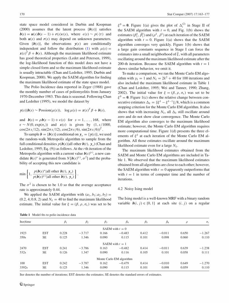
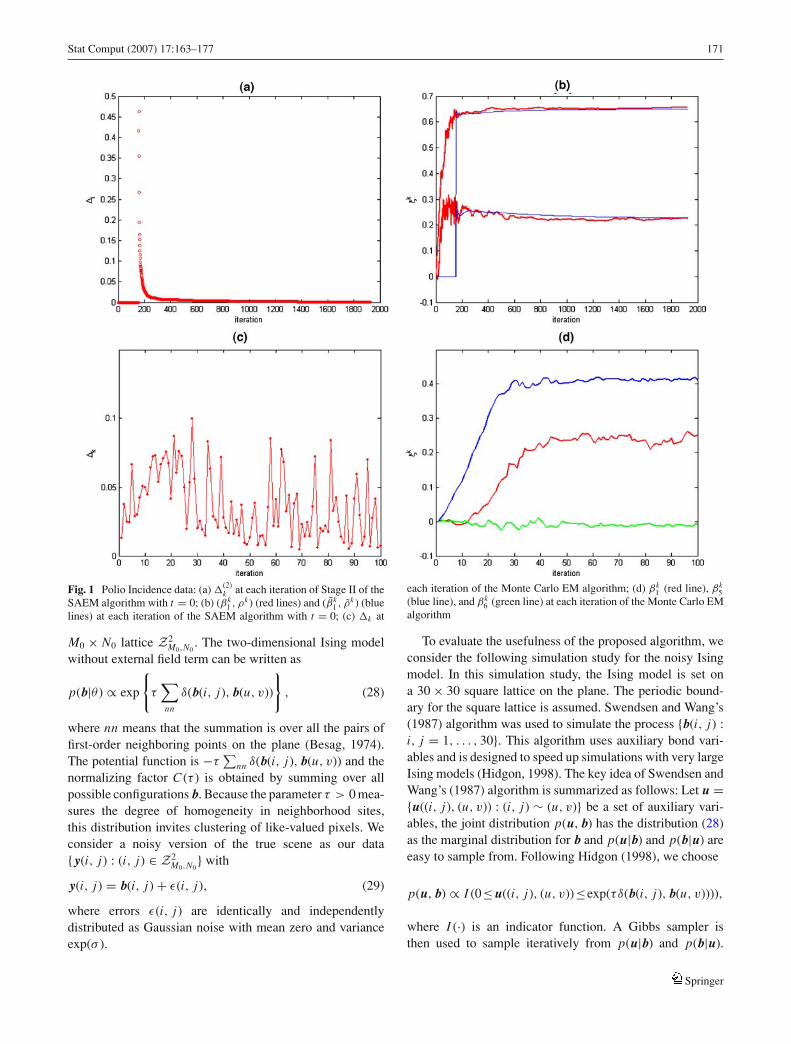
We applied the SAEM algorithm with (a1, b1; a2, b2) =(0.2, 4; 0.8, 2) and Nk = 40 to find the maximum likelihoodestimate. The initial value for ξ = (β, ρ, σε) was set to be

ξ 0 = 0. Figure 1(a) gives the plot of �(2)i in Stage II of

the SAEM algorithm with t = 0, and Fig. 1(b) shows theestimates (βk

1 , βk1 ) and (ρk, ρk) at each iteration of the SAEM

algorithm with t = 0. Figure 1(a) shows that the SAEMalgorithm converges very quickly. Figure 1(b) shows thata large gain constants sequence in Stage I can force theestimates into a small neighborhood of ξ , with all parametersoscillating around the maximum likelihood estimate after the200-th iteration. Because the SAEM algorithm with t = 1shows similar behavior, we omit it.

To make a comparison, we ran the Monte Carlo EM algo-rithm with γk = 1 and Nk = 2k2 + 40 for 100 iterations andalso included the maximum likelihood estimate in Table 1(Chan and Ledolter, 1995; Wei and Tanner, 1990; Zhang,2002). The initial value for ξ = (β, ρ, σε) was set to beξ 0 = 0. Figure 1(c) shows the relative change between con-secutive estimates �k = ‖ξ k − ξ k−1‖/8, which is a commonstopping criterion for the Monte Carlo EM algorithm. It alsoshows that with increasing Nk , all �k still oscillate aroundzero and do not show clear convergence. The Monte CarloEM algorithm also converges to the maximum likelihoodestimate; however, the Monte Carlo EM algorithm requiresmore computational time. Figure 1(d) presents the three el-ements of ξ k at each iteration of the Monte Carlo EM al-gorithm. All those estimates oscillate around the maximumlikelihood estimate even for a large Nk .

The maximum likelihood estimates obtained from theSAEM and Monte Carlo EM algorithms are included in Ta-ble 1. We observed that the maximum likelihood estimatesobtained from all algorithms are close to each other; however,the SAEM algorithm with t = 0 apparently outperforms thatwith t = 1 in terms of computer time and the number ofiterations.

4.2 Noisy Ising model

The Ising model is a well-known MRF with a binary randomvariable b(i, j) ∈ {0, 1} at each site (i, j) on a regular

Table 1 Model fits to polio incidence data

Iter/time β1 β2 β3 β4 β5 β6 ρ σε

SAEM with t = 01923 EST 0.228 −3.717 0.166 −0.483 0.412 −0.011 0.650 −1.267350s SE 0.125 1.346 0.090 0.115 0.101 0.098 0.060 0.110

SAEM with t = 12470 EST 0.241 −3.786 0.163 −0.482 0.414 −0.011 0.639 −1.238532s SE 0.126 1.347 0.090 0.116 0.105 0.101 0.058 0.111

Monte Carlo EM algorithm100 EST 0.242 −3.787 0.162 −0.479 0.414 −0.010 0.649 −1.2703392s SE 0.125 1.346 0.090 0.115 0.101 0.098 0.059 0.110

Iter denotes the number of iterations; EST denotes the estimates; SE denotes the standard errors of estimates.

Springer

Stat Comput (2007) 17:163–177 171

Fig. 1 Polio Incidence data: (a) �(2)k at each iteration of Stage II of the

SAEM algorithm with t = 0; (b) (βk1 , ρk ) (red lines) and (βk

1 , ρk ) (bluelines) at each iteration of the SAEM algorithm with t = 0; (c) �k at

each iteration of the Monte Carlo EM algorithm; (d) βk1 (red line), βk

5(blue line), and βk

6 (green line) at each iteration of the Monte Carlo EMalgorithm

M0 × N0 lattice Z2M0,N0

. The two-dimensional Ising modelwithout external field term can be written as

p(b|θ ) ∝ exp

{τ∑

nn

δ(b(i, j), b(u, v))

}, (28)

where nn means that the summation is over all the pairs offirst-order neighboring points on the plane (Besag, 1974).The potential function is −τ

∑nn δ(b(i, j), b(u, v)) and the

normalizing factor C(τ ) is obtained by summing over allpossible configurations b. Because the parameter τ > 0 mea-sures the degree of homogeneity in neighborhood sites,this distribution invites clustering of like-valued pixels. Weconsider a noisy version of the true scene as our data{ y(i, j) : (i, j) ∈ Z2

M0,N0} with

y(i, j) = b(i, j) + ε(i, j), (29)

where errors ε(i, j) are identically and independentlydistributed as Gaussian noise with mean zero and varianceexp(σ ).

To evaluate the usefulness of the proposed algorithm, weconsider the following simulation study for the noisy Isingmodel. In this simulation study, the Ising model is set ona 30 × 30 square lattice on the plane. The periodic bound-ary for the square lattice is assumed. Swendsen and Wang’s(1987) algorithm was used to simulate the process {b(i, j) :i, j = 1, . . . , 30}. This algorithm uses auxiliary bond vari-ables and is designed to speed up simulations with very largeIsing models (Hidgon, 1998). The key idea of Swendsen andWang’s (1987) algorithm is summarized as follows: Let u ={u((i, j), (u, v)) : (i, j) ∼ (u, v)} be a set of auxiliary vari-ables, the joint distribution p(u, b) has the distribution (28)as the marginal distribution for b and p(u|b) and p(b|u) areeasy to sample from. Following Hidgon (1998), we choose

p(u, b) ∝ I (0≤u((i, j), (u, v))≤exp(τδ(b(i, j), b(u, v)))),

where I (·) is an indicator function. A Gibbs sampler isthen used to sample iteratively from p(u|b) and p(b|u).

Springer

172 Stat Comput (2007) 17:163–177

The initial state of the process is taken at random suchthat b(i, j) is independently {0, 1} with equal probability.Swendsen and Wang’s (1987) algorithm was repeated 4000times to ensure that the equilibrium states were achievedand Gaussian noise with mean zero and variance exp(−0.5)was added to produce a “noisy” dataset.

We simulated 500 datasets for each parameter valueτ0 ∈ {0.2, 0.4, 0.6, 0.8}. Based on the simulated datasets,we applied the SAEM algorithm with t = 0 as describedin Section 3 to obtain the maximum likelihood estimate ofξ = (τ, σ ). The starting value of ξ 0 was taken to be (0.1, 0.0).The SAEM algorithm with (a1, b1; a2, b2) = (0.4, 5; 0.8, 2)converged quickly. In order to estimate ∂τ log C(τ ) and∂2τ log C(τ ), the Metropolis algorithm (Gu and Zhu, 2001)

was applied at each site (i, j) to generate b from (28) in eachiteration of the SAEM algorithm.

To simulate the random sample from b conditional on yo,we used the following Metropolis algorithm. Let the currentvalue of the process at site (l, j) be b(l, j) and the currentvalue of the potential function be U . Take the alternativevalue b(l, j)∗ at the site (l, j), which leads to the value of thepotential function U ∗, the probability of accepting this newcandidate b(l, j)∗ and U ∗ is

min{1, exp{(U − U ∗) + 0.5[ y(l, j) − b(l, j)]2

× exp(−σ ) − 0.5[ y(l, j) − b(l, j)∗]2 exp(−σ )}}.Moreover, each site was selected at random with

1/(30 × 30) probability not according to the lexicographicalorder. For example, if site (1,1) was selected, we ran theabove mentioned Metropolis procedure at the site (1,1)with other sites unchanged. Thus, only the value at onesite can change from bk,i−1 to bk,i . The number Nk was setat Nk = 20000. Compared with the total number of sites30 × 30 = 900, Nk = 20000 is not exceedingly large.

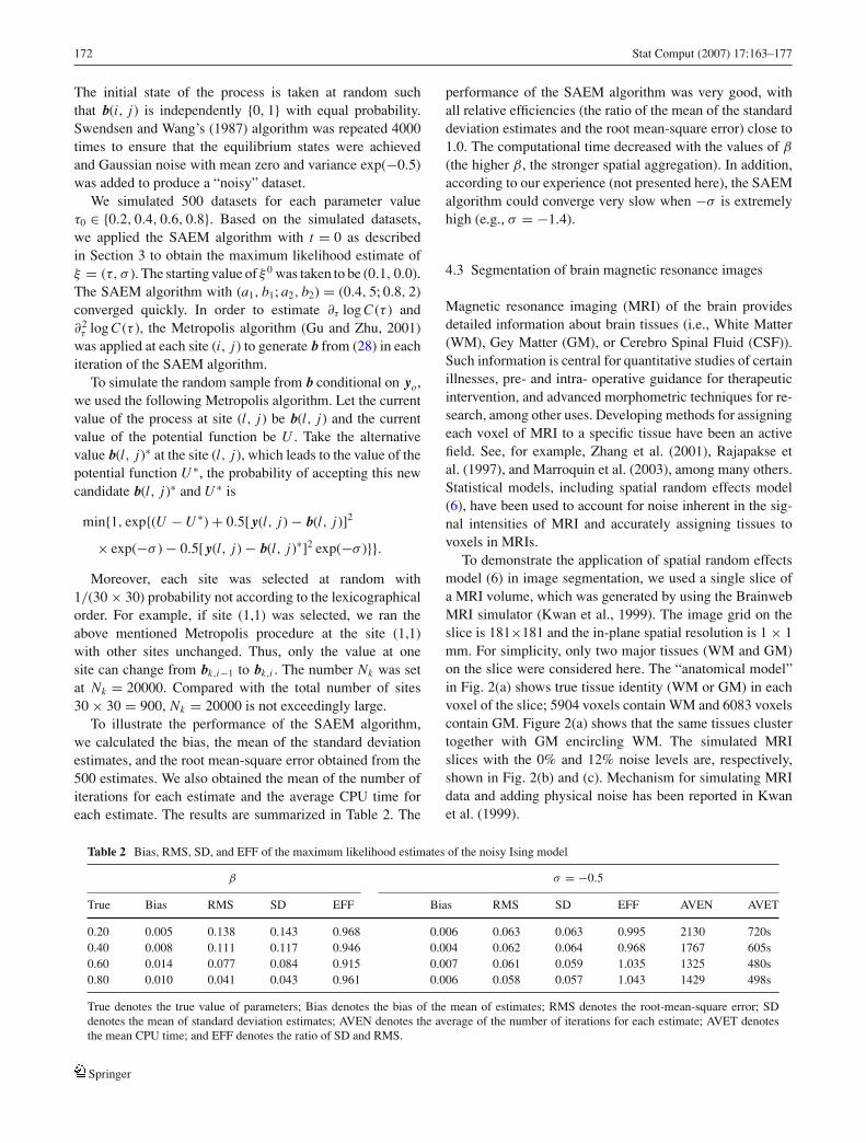
To illustrate the performance of the SAEM algorithm,we calculated the bias, the mean of the standard deviationestimates, and the root mean-square error obtained from the500 estimates. We also obtained the mean of the number ofiterations for each estimate and the average CPU time foreach estimate. The results are summarized in Table 2. The

performance of the SAEM algorithm was very good, withall relative efficiencies (the ratio of the mean of the standarddeviation estimates and the root mean-square error) close to1.0. The computational time decreased with the values of β

(the higher β, the stronger spatial aggregation). In addition,according to our experience (not presented here), the SAEMalgorithm could converge very slow when −σ is extremelyhigh (e.g., σ = −1.4).

4.3 Segmentation of brain magnetic resonance images

Magnetic resonance imaging (MRI) of the brain providesdetailed information about brain tissues (i.e., White Matter(WM), Gey Matter (GM), or Cerebro Spinal Fluid (CSF)).Such information is central for quantitative studies of certainillnesses, pre- and intra- operative guidance for therapeuticintervention, and advanced morphometric techniques for re-search, among other uses. Developing methods for assigningeach voxel of MRI to a specific tissue have been an activefield. See, for example, Zhang et al. (2001), Rajapakse etal. (1997), and Marroquin et al. (2003), among many others.Statistical models, including spatial random effects model(6), have been used to account for noise inherent in the sig-nal intensities of MRI and accurately assigning tissues tovoxels in MRIs.

To demonstrate the application of spatial random effectsmodel (6) in image segmentation, we used a single slice ofa MRI volume, which was generated by using the BrainwebMRI simulator (Kwan et al., 1999). The image grid on theslice is 181×181 and the in-plane spatial resolution is 1 × 1mm. For simplicity, only two major tissues (WM and GM)on the slice were considered here. The “anatomical model”in Fig. 2(a) shows true tissue identity (WM or GM) in eachvoxel of the slice; 5904 voxels contain WM and 6083 voxelscontain GM. Figure 2(a) shows that the same tissues clustertogether with GM encircling WM. The simulated MRIslices with the 0% and 12% noise levels are, respectively,shown in Fig. 2(b) and (c). Mechanism for simulating MRIdata and adding physical noise has been reported in Kwanet al. (1999).

Table 2 Bias, RMS, SD, and EFF of the maximum likelihood estimates of the noisy Ising model

β σ = −0.5

True Bias RMS SD EFF Bias RMS SD EFF AVEN AVET

0.20 0.005 0.138 0.143 0.968 0.006 0.063 0.063 0.995 2130 720s0.40 0.008 0.111 0.117 0.946 0.004 0.062 0.064 0.968 1767 605s0.60 0.014 0.077 0.084 0.915 0.007 0.061 0.059 1.035 1325 480s0.80 0.010 0.041 0.043 0.961 0.006 0.058 0.057 1.043 1429 498s

True denotes the true value of parameters; Bias denotes the bias of the mean of estimates; RMS denotes the root-mean-square error; SDdenotes the mean of standard deviation estimates; AVEN denotes the average of the number of iterations for each estimate; AVET denotesthe mean CPU time; and EFF denotes the ratio of SD and RMS.

Springer

Stat Comput (2007) 17:163–177 173

Fig. 2 Segmentation of MRI data: an anatomical model giving trueidentity (White Matter (colored red) or Grey Matter (colored white))in each voxel of the MRI slice (a); the simulated MRI slice with the0 percent noise (b, d, and f); and the simulated MRI slice with the 12percent noise (c, e, and g). For the MRI slice with 0 percent noise, weshow the raw data in (b), the estimated anatomical model from mixture

model in (d), and the estimated anatomical model from spatial randomeffects model and by using ICM in (f). For the MRI slice with 12 per-cent noise, we show the raw data in (c), the estimated anatomical modelfrom mixture model in (e), and the estimated anatomical model fromspatial random effects model and by using ICM in (g)

Given the ground truth in Fig. 2(a), we performed somepreliminary analyses on the MRI slice with different noiselevels. For the slice with the 0% noise level, we calculated themean and standard deviation of image intensities for WM as(702.462, 31.335), and those for GM as (530.245, 51.133).However, for the slice with the 12% noise level, the mean andstandard deviation of image intensities for WM and GM are,respectively, (809.397, 173.675) and (612.819, 171.809).

We used a mixture normal model to cluster two tissues(GM and WM) on the two simulated MRI slices. The signalintensity y(si ) at each voxel si can be written as

y(si ) =2∑

k=1

[β(k) + εk(si )]δ(b(si ), k), (30)

where β(1) and β(2) denote, respectively, the mean sig-nal intensities of WM and GM, εk(si ) follows the nor-mal distribution with zero mean and variance exp(σk)for k = 1 and 2, and b(si ) = 1 (or 2) represents un-known tissue type WM (or GM). Furthermore, all b(si )are binary variables and identically and independently dis-tributed. In addition, P(b(si ) = 1) = 1/[1 + exp(τ1(2))] andP(b(si ) = 2) = exp(τ1(2))/[1 + exp(τ1(2))]. The unknownparameter vector ξ for the mixture model is given byξ = (β(1), σ1, β(2), σ2, τ1(2))T . Given the maximum likeli-hood estimate ξ , we can obtain an estimate of the conditionalprobability P(b(si ) = 1|ξ ) at each si as follow:

φ( y(si ); β(1), σ1)

φ( y(si ); β(1), σ1) + φ( y(si ); β(2), σ2) exp(τ1(2)),

Springer

174 Stat Comput (2007) 17:163–177

where φ( y(si ); β, σ ) = exp(−0.5σ − 0.5( y(si ) − β)2/ exp(σ )). Then, we can compute the sum of the correct prediction(SCP) as follow:

SCP =n∑

i=1

δ(b(si )

true, b(si )pred)

(31)

where n = 11987, b(si )true denotes the true b(si ), andb(si )pred equals 1 when P(b(si ) = 1|ξ ) > 0.5 and 2 other-wise.

For the MRI slice with the 0% noise level, we ap-plied the expectation-maximization algorithm to find ξ =(713.068, 5.983, 548.409, 8.355, 0.385)T with SCP = 906.For the MRI slice with the 12% noise level, ξ is (808.591,

10.358, 604.351, 10.183,−0.062)T with SCP = 3371. Wepresent bpred for both MRI slices in Fig. 2(d) and (e). Asexpected, higher levels of noise leads to larger SCPs. More-over, for data with high levels of noise, the mixture modelcannot recover the cohesion of the same tissues.

We applied model (6) to cluster two tissues (WM and GM)on the MRI slices with differing noise levels, and we calcu-lated ξ by using the SAEM algorithm. Because S in Fig. 2(a)is an irregular lattice, we consider the joint distribution ofthe site responses b = {b(si ) : si ∈ S} conditional upon re-sponses bO = {b(si ) : si ∈ SO}, where SO and S denote theset of all sites forming the outside of S and the set of all sitesof S, respectively. Furthermore, we assume that all b(si ) forsi ∈ SO equal 2, which requires that the tissues close to theboundary are GM, although we only use information fromthe voxels near the boundary of S. We assume model (31),but the joint distribution of the latent field b given bO can bewritten as

exp

{τ1(2)

n∑

i=1

δ(b(si ), 2) + τ2

∑

si ∼s j

δ(b(si ), b(s j ))

− log C(τ1(2), τ2)

}, (32)

where the first-order neighboring correlation is used (Hufferand Wu, 1998). The unknown parameter vector ξ is (β1,

σ1, β2, σ2, τ1(2), τ2)T .To estimate ∂τ log C(τ ) and ∂2

τ log C(τ ), we applied theMetropolis algorithm at each site si to generate b from (32) ineach iteration of the proposed algorithm (Gu and Zhu, 2001).To simulate the random sample from b conditional on yo andbO , the following Metropolis algorithm was used. We call itSampling Method (I). Let the current value of the process atsite si be b(si ) and the current value of the potential functionis denoted as U . Take the alternative value b(si )∗ at the sitesi which leads to the value of the potential function U ∗, theprobability of accepting this new candidate b(si )∗ and U ∗ is

min{1, exp{(U − U ∗) + 0.5[y(si ) − β(k)]2e−σk

−0.5[y(si ) − β(m)]2e−σm + 0.5[σk − σm]}},

where b(si ) = k and b(s∗i ) = m. Moreover, each site was

selected at random with 1/n = 1/11987 probability. Thenumber Nk was set at Nk = 60, 000, which is about fivetimes the number of sites in S.

For the two simulated MRI slices with differing noise lev-els, we applied the SAEM algorithm with (a1, b1; a2, b2) =(0.2, 5; 0.8, 2) and t = 0 to find the maximum likeli-hood estimate of spatial random effects model (6). Forthe MRI slice with the 0% noise level, ξ 0 was set at(713.07, 5.98, 548.41, 8.36, 0.39, 0.0, 1.0)T and the SAEMalgorithm took 4032 iterations to obtain

ξ T = (710.78, 6.18, 541.70, 8.17,−3.62, 1.84)

with standard errors (0.84, 0.02, 0.39, 0.03, 0.02, 0.01).Given the maximum likelihood estimate ξ , we appliedthe iterated conditional modes (ICM) to obtain an es-timate of bpred and the value of SCP as 695. Recallthat SCP = 906 based on the mixture model. We presentbpred in Fig. 2(f). For the MRI slice with the 12%noise level, the SAEM algorithm starts from initial valueξ 0 = (713.07, 5.98, 548.41, 8.36, 0.39, 0.0, 1.0)T and con-verges to ξ T = (823.79, 10.19, 582.06, 10.04,−3.50, 1.77)with standard errors (2.89, 0.02, 2.90, 0.02, 0.01, 0.01) in2393 iterations. We then applied ICM to estimate bpred;see Fig. 2(g). Moreover, the value of SCP = 1463 is muchsmaller than SCP = 3371 based on the mixture model de-scribed above. It reveals that introducing spatial correlationtruly improves performance of the segregation methods.

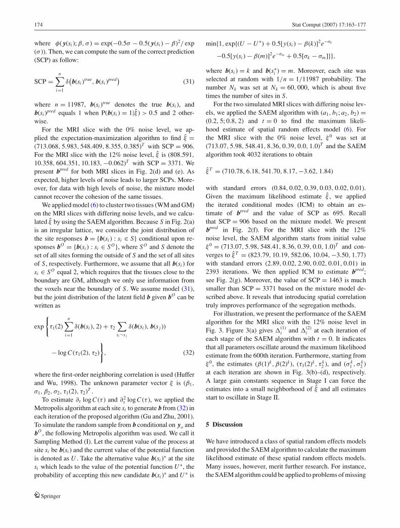
For illustration, we present the performance of the SAEMalgorithm for the MRI slice with the 12% noise level inFig. 3. Figure 3(a) gives �

(1)i and �

(2)i at each iteration of

each stage of the SAEM algorithm with t = 0. It indicatesthat all parameters oscillate around the maximum likelihoodestimate from the 600th iteration. Furthermore, starting fromξ 0, the estimates (β(1)k, β(2)k), (τ1(2)k, τ k

2 ), and (σ k1 , σ k

2 )at each iteration are shown in Fig. 3(b)–(d), respectively.A large gain constants sequence in Stage I can force theestimates into a small neighborhood of ξ and all estimatesstart to oscillate in Stage II.

5 Discussion

We have introduced a class of spatial random effects modelsand provided the SAEM algorithm to calculate the maximumlikelihood estimate of these spatial random effects models.Many issues, however, merit further research. For instance,the SAEM algorithm could be applied to problems of missing

Springer

Stat Comput (2007) 17:163–177 175

Fig. 3 Segmentation of MRI data: (a) �(1)k (blue line) and �

(2)k (red

line) at each iteration of Stages I and II of the SAEM algorithm; (b) βk1

(red line) and βk2 (blue line) at each iteration; (c) τ1(2)k (red line) and

τ k2 (blue line) at each iteration; (d) σ k

1 (red line) and σ k2 (blue line) at

each iteration

data, such as those found in generalized linear mixed mea-surement error models (Wang et al., 1998), parametric re-gression models with missing covariates (Horton and Laird,1998), and generalized nonparametric mixed effects models(Karcher and Wang, 2001). The SAEM algorithm shouldprovide an efficient algorithm for finding the maximum like-lihood estimate of those models for missing data. Pairwiseinteraction Markov Random Fields are another widely usedclass of distributions in spatial statistics (Besag et al., 1995);spatial random effects models, however, exclude this model,because we assume that the sites of latent process of b are pre-determined and non-random. Future work applying SAEMalgorithms to the pairwise interaction MRFs will need todevelop an efficient algorithm for sampling from the latentprocess. Further research should also calculate Bayesian esti-mates of spatial random effects models. Here, sampling from

the distribution of parameters associated with the normaliz-ing factor of MRFs will be the primary difficulty (Liu, 2001).

Acknowledgments This work was supported in part by NSF grant SES-0643663 to Dr. Zhu, Hong Kong Research Grants Council competitive grant216078 to Dr. Gu, NIDA grant DA017820, NIMH grants MH068318 andK0274677 to Dr. Peterson, by the Suzanne Crosby Murphy Endowment atColumbia University Medical Center, and by the Thomas D. Klingensteinand Nancy D. Perlman Family Fund. We thank the Editor, an Associate Ed-itor, and three anonymous referees for valuable suggestions, which greatlyhelped improve our presentation. Thanks to Dr. Jason Royal for his invalu-able editorial assistance.

References

Aitkin M. 1996. A general maximum likelihood analysis of overdis-persion in generalized linear models. Statistics and Computing 6:251–262.

Springer

176 Stat Comput (2007) 17:163–177

Benveniste A., Metivier M., and Priouret P. 1990. Adaptive Algorithmsand Stochastic Approximations. Springer-Verlag, New York.

Besag J.E. 1974. Spatial interaction and the statistical analysis oflattice systems (with discussion). Journal of Royal StatisticalSociety, Series B 36: 192–236.

Besag J.E. 1986. On the statistical analysis of dirty pictures (withdiscussion). Journal of Royal Statistical Society, Series B 48:259–302.

Besag J.E., Green P., Higdon D., and Mengersen K. 1995. Bayesiancomputation and stochastic systems (with discussion). StatisticalScience 10: 3–66.

Breslow N.E. and Clayton D.G. 1993. Approximate inference ingeneralized linear mixed models. Journal of American StatisticalAssociation 88: 9–25.

Chan K.S. and Ledolter J. 1995. Monte Carlo EM estimation for timeseries models involving counts. Journal of American StatisticalAssociation 90: 242–252.

Christensen O.F. and Waagepetersen R.P. 2002. Bayesian predictionof spatial count data using generalized linear mixed models.Biometrics 58: 280–286.

Delyon B., Lavielle E., and Moulines E. 1999. Convergence of astochastic approximation version of the EM algorithm. Annals ofStatistics 27: 94–128.

Derin H. and Elliott H. 1987. Modeling and segmentation of noisy andtextured images using Gibbs random fields. IEEE Transactionson Pattern Analysis and Machine Intelligence 9: 39–55.

Diggle P.J., Tawn J.A., and Moyeed R.A. 1998. Model-basedgeostatistics (with discussion). Applied Statistics 47: 299–350.

Durbin J. and Koopman S.J. 1997. Monte Carlo maximum likelihoodestimation for non-Gaussian state space models. Biometrika 84:669–684.

Durbin J. and Koopman S.J. 2000. Time series analysis of non-Gaussian observations based on state space models from bothclassical and Bayesian perspectives (with discussion). Journal ofRoyal Statistical Society, Series B 62: 3–56.

Gelman A. and Meng X.L. 1998. Simulating normalizing constants:from importance sampling to bridge sampling to path sampling.Statistical Science 13: 163–185.

Geman S. and Geman D. 1984. Stochastic relaxation, Gibbsdistribution, and the Bayesian restoration of images. IEEE Trans-actions on Pattern Analysis and Machine Intelligence 6: 721–741.

Geyer C.J. and Thompson E.A. 1992. Constrained Monte Carlomaximum likelihood for dependent data (with discussion).Journal of Royal Statistical Society, Series B 54: 657–699.

Gu M.G. and Kong F.H. 1998. A stochastic approximation algorithmwith Markov chain Monte Carlo method for incomplete dataestimation problems. In: Proceeding of National AcademicScience of USA 95: 7270–7274.

Gu M.G. and Zhu H.T. 2001. Maximum likelihood estimation for spatialmodels by Markov chain Monte Carlo stochastic approximation.Journal of Royal Statistical Society, Series B 63: 339–355.

Higdon D.M. 1998. Auxiliary variable methods for Markov chainMonte Carlo with applications. Journal of American StatisticalAssociation 93: 585–595.

Horton N.J. and Laird N.M. 1998. Maximum likelihood analysis ofgeneralized linear models with missing covariates. StatisticalMethods in Medical Research 8: 37–50.

Huang F. and Ogata Y. 2001. Comparison of two methods for calcu-lating the partition functions of various spatial statistical models.The Australian and New Zealand Journal of Statistics 43: 47–65.

Huffer F.W. and Wu H.L. 1998. Markov chain Monte Carlo for auto-logistic regression models with application to the distribution ofplant species. Biometrics 54: 509–524.

Jens L.J. and Niels V.P. 1999. Asymptotic normality of the maximumlikelihood estimator in state space models. Annals of Statistics27: 514–535.

Karcher P. and Wang Y. 2001. Generalized nonparametric mixedeffects models. Journal of Computational and Graphical Statistics10: 641–655.

Kwan R.K.S., Evans A.C., and Pike G.B. 1999. MRI simulation-basedevaluation of image-processing and classification methods. IEEETransactions on Medical Imaging 18: 1085–1097.

Lai T.L. 2003. Stochastic approximation. Annals of Statistics 31:391–406.

Lange K. 1995. A gradient algorithm locally equivalent to the EM algo-rithm. Journal of Royal Statistical Society, Series B 55: 425–437.

Lee Y. and Nelder J.A. 1996. Hierarchical generalized linear models(with discussion). Journal of Royal Statistical Society, Series B58: 619–678.

Li S.Z. 2001. Markov Random Field Modeling in Image Analysis.Springer-Verlag, Tokyo.

Liu J. 2001. Monte Carlo Strategies in Scientific Computing. Springer,New York.

Louis T.A. 1982. Finding the observed information matrix when usingthe EM algorithm. Journal of Royal Statistical Society, Series B44: 190–200.

Marroquin J.L., Santana E.A., and Botello S. 2003. Hidden Markovmeasure field models for image segmentation. IEEE Transactionson Pattern Analysis and Machine Intelligence 25: 1380–1397.

McCullagh P. and Nelder J.A. 1989. Generalized Linear Models (2ndedn.). Chapman and Hall, London.

Møller J. 1999. Markov chain Monte Carlo and spatial point processes.In W.S. Kendall, O.E. Barndorff-Nielsen, and M.C. van Lieshout(Eds.), Stochastic Geometry: Likelihood and Computation,Chapman and Hall, London.

Moyeed R.A. and Baddeley A.J. 1991. Stochastic approximation ofthe maximum likelihood estimate for a spatial point pattern.Scandinavian Journal of Statistics 18: 39–50.

Ortega J.M. 1990. Numerical Analysis: A Second Course. Society forIndustrial and Academic Press, Philadelphia.

Penttinen A. 1984. Modelling interaction in spatial point patterns:parameter estimation by the maximum likelihood method. Jy.Stud. Comput. Sci. Econometr. Statist. 7.

Pettitt A.N., Friel N., and Reeves R. 2003. Efficient calculation of thenormalisation constant of the autologistic model on the lattice.Journal of Royal Statistical Society, Series B 65: 235–247.

Polyak B.T. 1990. New stochastic approximation type procedures.Autom. Telem. pp. 98–107. (English translation in Automat.Remote Contr. 51).

Polyak B.T. and Juditski A.B. 1992. Acceleration of stochasticapproximation by averaging. SIAM Journal of Control andOptimization 30: 838–855.

Qian W. and Titterington D.M. 1991. Estimation of parameters inhidden Markov models. Philosophical Transactions of the RoyalSociety of London, Series A 337: 407–428.

Rajapakse J.C., Giedd J.N., and Rapoport J.L. 1997. Statisticalapproach to segmentation of single-channel cerebral MR images.IEEE Transactions on Medical Imaging 16: 176–186.

Robbins H. and Monro S. 1951. A stochastic approximation method.Annals of Mathematical Statistics 22: 400–407.

Robert C.P. and Casella G. 1999. Monte Carlo Statistical Methods.Springer-Verlag, New York.

Ryden T. 1997. On recursive estimation for hidden Markov models.Stochastic Processes and their Applications 66: 79–96.

Saquib S.S., Bouman C.A., and Sauer K. 1998. ML parameter esti-mation for Markov random fields with applications to Bayesiantomography. Transactions on Image Processing 7: 1029–1044.

Springer

Stat Comput (2007) 17:163–177 177

Stoer J. and Bulisch R. 1980. Introduction to Numerical Analysis.Springer-Verlag, New York.

Swendsen R.H. and Wang J.S. 1987. Nonuniversal critical dynamicsin Monte Carlo simulation. Physics Review Letters 58: 86–88.

Wang N., Lin X., Gutierrez R.G., and Carroll R.J. 1998. Bias analysisand SIMEX approach in generalized linear mixed measurementerror models. Journal of American Statistical Association 93:249–261.

Wei G.C.G. and Tanner M.A. 1990. A Monte Carlo implementationof the EM algorithm and the Poor man’s data augmentationalgorithm. Journal of American Statistical Association 85: 699–704.

Winkler G. 1995. Image Analysis, Random Fields and Dynamic MonteCarlo Methods: A Mathematical Introduction. Springer-Verlag,Berlin Heidelberg.

Younes L. 1989. Parameter estimation for imperfectly observedGibbsian fields. Probability Theory Related Feilds 82: 625–645.

Zeger S.L. 1988. A regression model for time series of counts.Biometrika 75: 621–629.

Zeger S.L., Liang K.Y., and Albert P.S. 1988. Models for longitudinaldata: a generalized estimating equation approach. Biometrics 44:1049–1060.

Zhang H. 2002. On estimation and prediction for spatial generalizedlinear mixed models. Biometrics 56: 129–136.

Zhang Y., Brady M., and Smith S. 2001. Segmentation of brainMR images through a hidden Markov random field model andthe expectation-maximization algorithm. IEEE Transactions onMedical Imaging 15: 45–57.

Zhu H.T. and Gu M.G. 2005. Maximum likelihood from spatial randomeffects models via the stochastic approximation expectation max-imization algorithm (supplement). Technical report, Departmentof Biostatistics, University of North Carolina at Chapel Hill.

Zhu H.T. and Lee S.Y. 2002. Analysis of generalized linear mixed mod-els via a stochastic approximation algorithm with Markov chainMonte Carlo method. Statistics and Computing 12: 175–183.

Zhu H.T. and Zhang H.P. 2004. Hypothesis testing in a class of mixtureregression models. Journal of Royal Statistical Society, Series B:66: 3–16.

Springer