Neural repetition suppression: evidence for perceptual expectation in object-selective regions
Upload
khangminh22Category
view
3download
0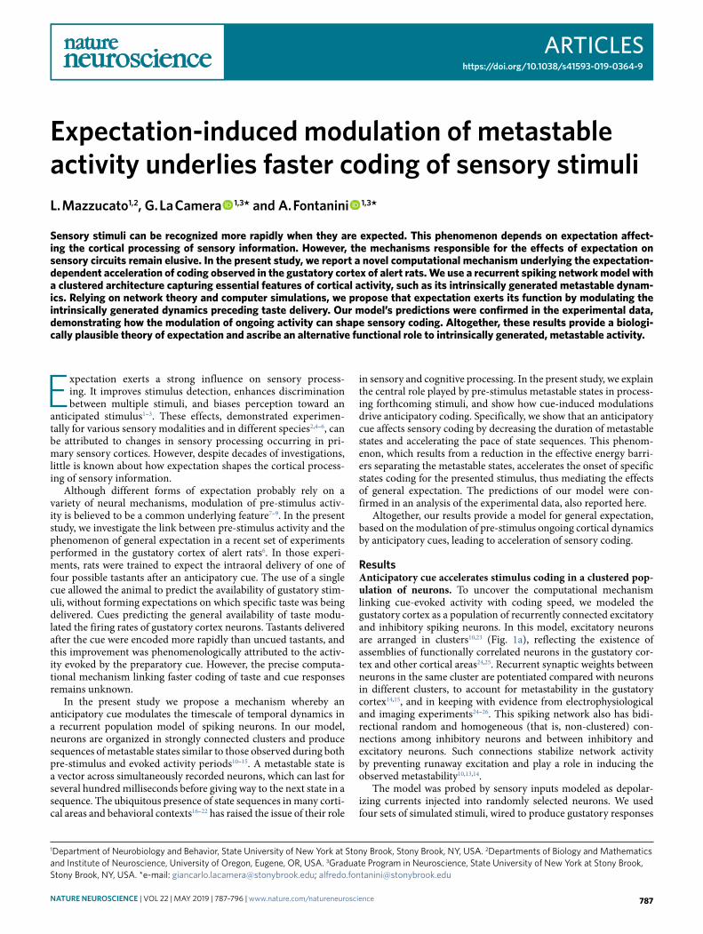
Articleshttps://doi.org/10.1038/s41593-019-0364-9
1Department of Neurobiology and Behavior, State University of New York at Stony Brook, Stony Brook, NY, USA. 2Departments of Biology and Mathematics and Institute of Neuroscience, University of Oregon, Eugene, OR, USA. 3Graduate Program in Neuroscience, State University of New York at Stony Brook, Stony Brook, NY, USA. *e-mail: [email protected]; [email protected]
Expectation exerts a strong influence on sensory process-ing. It improves stimulus detection, enhances discrimination between multiple stimuli, and biases perception toward an
anticipated stimulus1–3. These effects, demonstrated experimen-tally for various sensory modalities and in different species2,4–6, can be attributed to changes in sensory processing occurring in pri-mary sensory cortices. However, despite decades of investigations, little is known about how expectation shapes the cortical process-ing of sensory information.
Although different forms of expectation probably rely on a variety of neural mechanisms, modulation of pre-stimulus activ-ity is believed to be a common underlying feature7–9. In the present study, we investigate the link between pre-stimulus activity and the phenomenon of general expectation in a recent set of experiments performed in the gustatory cortex of alert rats6. In those experi-ments, rats were trained to expect the intraoral delivery of one of four possible tastants after an anticipatory cue. The use of a single cue allowed the animal to predict the availability of gustatory stim-uli, without forming expectations on which specific taste was being delivered. Cues predicting the general availability of taste modu-lated the firing rates of gustatory cortex neurons. Tastants delivered after the cue were encoded more rapidly than uncued tastants, and this improvement was phenomenologically attributed to the activ-ity evoked by the preparatory cue. However, the precise computa-tional mechanism linking faster coding of taste and cue responses remains unknown.
In the present study we propose a mechanism whereby an anticipatory cue modulates the timescale of temporal dynamics in a recurrent population model of spiking neurons. In our model, neurons are organized in strongly connected clusters and produce sequences of metastable states similar to those observed during both pre-stimulus and evoked activity periods10–15. A metastable state is a vector across simultaneously recorded neurons, which can last for several hundred milliseconds before giving way to the next state in a sequence. The ubiquitous presence of state sequences in many corti-cal areas and behavioral contexts16–22 has raised the issue of their role
in sensory and cognitive processing. In the present study, we explain the central role played by pre-stimulus metastable states in process-ing forthcoming stimuli, and show how cue-induced modulations drive anticipatory coding. Specifically, we show that an anticipatory cue affects sensory coding by decreasing the duration of metastable states and accelerating the pace of state sequences. This phenom-enon, which results from a reduction in the effective energy barri-ers separating the metastable states, accelerates the onset of specific states coding for the presented stimulus, thus mediating the effects of general expectation. The predictions of our model were con-firmed in an analysis of the experimental data, also reported here.
Altogether, our results provide a model for general expectation, based on the modulation of pre-stimulus ongoing cortical dynamics by anticipatory cues, leading to acceleration of sensory coding.
ResultsAnticipatory cue accelerates stimulus coding in a clustered pop-ulation of neurons. To uncover the computational mechanism linking cue-evoked activity with coding speed, we modeled the gustatory cortex as a population of recurrently connected excitatory and inhibitory spiking neurons. In this model, excitatory neurons are arranged in clusters10,23 (Fig. 1a), reflecting the existence of assemblies of functionally correlated neurons in the gustatory cor-tex and other cortical areas24,25. Recurrent synaptic weights between neurons in the same cluster are potentiated compared with neurons in different clusters, to account for metastability in the gustatory cortex14,15, and in keeping with evidence from electrophysiological and imaging experiments24–26. This spiking network also has bidi-rectional random and homogeneous (that is, non-clustered) con-nections among inhibitory neurons and between inhibitory and excitatory neurons. Such connections stabilize network activity by preventing runaway excitation and play a role in inducing the observed metastability10,13,14.
The model was probed by sensory inputs modeled as depolar-izing currents injected into randomly selected neurons. We used four sets of simulated stimuli, wired to produce gustatory responses
Expectation-induced modulation of metastable activity underlies faster coding of sensory stimuliL. Mazzucato1,2, G. La Camera 1,3* and A. Fontanini 1,3*
Sensory stimuli can be recognized more rapidly when they are expected. This phenomenon depends on expectation affect-ing the cortical processing of sensory information. However, the mechanisms responsible for the effects of expectation on sensory circuits remain elusive. In the present study, we report a novel computational mechanism underlying the expectation-dependent acceleration of coding observed in the gustatory cortex of alert rats. We use a recurrent spiking network model with a clustered architecture capturing essential features of cortical activity, such as its intrinsically generated metastable dynam-ics. Relying on network theory and computer simulations, we propose that expectation exerts its function by modulating the intrinsically generated dynamics preceding taste delivery. Our model’s predictions were confirmed in the experimental data, demonstrating how the modulation of ongoing activity can shape sensory coding. Altogether, these results provide a biologi-cally plausible theory of expectation and ascribe an alternative functional role to intrinsically generated, metastable activity.
NAtuRE NEuRosCiENCE | VOL 22 | MAY 2019 | 787–796 | www.nature.com/natureneuroscience 787
Articles NATuRe NeuROScIeNce
reminiscent of those observed in the experiments in the presence of sucrose, sodium chloride, citric acid, and quinine (see Methods). The specific connectivity pattern used was inferred by the pres-ence of both broadly and narrowly tuned responses in the gustatory cortex27,28, and the temporal dynamics of the inputs were varied to determine the robustness of the model (Fig. 2).
In addition to input gustatory stimuli, we included anticipa-tory inputs designed to produce cue responses analogous to those seen experimentally in the case of general expectation. To simu-late general expectation, we connected anticipatory inputs with random neuronal targets in the network. The peak value of the cue-induced current for each neuron was sampled from a normal distribution with zero mean and fixed variance, thus introducing a spatial variance in the afferent currents. This choice reflected the large heterogeneity of cue responses observed in the empirical data,
where excited and inhibited neural responses occurred in simi-lar proportions9 and overlapped partially with taste responses6,9. Figure 1b shows two representative cue-responsive neurons in the model: one inhibited by the cue and one excited by the cue. Cue responses in the model were in quantitative agreement with the observed responses for a large range of cue-induced spatial vari-ance (Supplementary Fig. 1; see Supplementary Fig. 2 for represen-tative unresponsive neurons).
Given these conditions, we simulated the experimental para-digm adopted in awake-behaving rats to demonstrate the effects of general expectation6,9. In the original experiment, rats were trained to self-administer into an intraoral cannula one of four possible tastants following an anticipatory cue. At random trials and time during the intertrial interval, tastants were unexpectedly delivered in the absence of a cue. To match this experiment, the simulated
Stimulus afferents
Cue afferents
a Cue-responsive neurons
Inhibited neuron
Excited neuron
Tria
ls
25 spks s–1
Model architecture
Clu
ster
ed n
etw
ork
Hom
ogen
eous
net
wor
k
Stimulus afferents
Cue afferents
Cue Stimulus
–0.5 0 0.5
b
10 spks s–1
20 spks s–1
Time (s)
–0.5 0 0.5
Inhibited neuron
Tria
ls
–0.5 0 0.5
Excited neuron
Cue Stimulus
Tria
lsTime (s)
–0.5 0 0.5
20 spks s–1
Tria
ls
d e
Stimulus codingc
–0.5 0 0.5
Time (s)
Cue Stimulus
–0.5 0 0.5
Time (s)
Cue Stimulus
f
Dec
odin
g ac
cura
cy (
%)
0
100
Dec
odin
g ac
cura
cy (
%)
0
100
ExpectedUnexpected
ExpectedUnexpected
Latency (s)
**
0
0.3
NS
Latency (s)
0
0.2
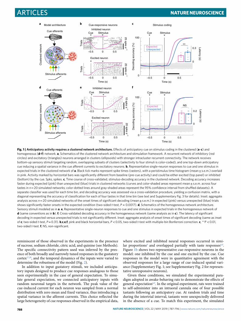
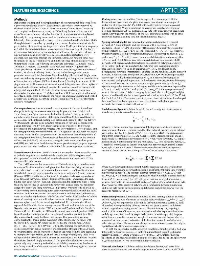
Fig. 1 | Anticipatory activity requires a clustered network architecture. Effects of anticipatory cue on stimulus coding in the clustered (a–c) and homogeneous (d–f) network. a, Schematics of the clustered network architecture and stimulation framework. A recurrent network of inhibitory (red circles) and excitatory (triangles) neurons arranged in clusters (ellipsoids) with stronger intracluster recurrent connectivity. The network receives bottom-up sensory stimuli targeting random, overlapping subsets of clusters (selectivity to four stimuli is color-coded), and one top-down anticipatory cue inducing a spatial variance in the cue afferent currents to excitatory neurons. b, Representative single-neuron responses to cue and one stimulus in expected trials in the clustered network of a. Black tick marks represent spike times (rasters), with a peristimulus time histogram (mean ± s.e.m.) overlaid in pink. Activity marked by horizontal bars was significantly different from baseline (pre-cue activity) and could be either excited (top panel) or inhibited (bottom) by the cue. Spks, spikes. c, Time course of cross-validated, stimulus-decoding accuracy in the clustered network. Decoding accuracy increases faster during expected (pink) than unexpected (blue) trials in clustered networks (curves and color-shaded areas represent mean ± s.e.m. across four tastes in n = 20 simulated networks; color-dotted lines around gray-shaded areas represent the 95% confidence interval from shuffled datasets). A separate classifier was used for each time bin, and decoding accuracy was assessed via a cross-validation procedure, yielding a confusion matrix, with a diagonal representing the accuracy of classification for each of four tastes in that time bin (see text and Supplementary Fig. 3 for details). Inset: aggregate analysis across n = 20 simulated networks of the onset times of significant decoding (mean ± s.e.m.) in expected (pink) versus unexpected (blue) trials shows significantly faster onsets in the expected condition (two-sided t-test, P = 0.0017). d, Schematics of the homogeneous network architecture. Sensory stimuli modeled as in a. e, Representative single-neuron responses to cue and one stimulus in expected trials in the homogeneous network of d (same conventions as in b). f, Cross-validated decoding accuracy in the homogeneous network (same analysis as in c). The latency of significant decoding in expected versus unexpected trials is not significantly different. Inset: aggregate analysis of onset times of significant decoding (same as inset of c; two-sided t-test, P = 0.31). b,c,e,f, pink and black horizontal bars, P < 0.05, two-sided t-test with multiple-bin Bonferroni correction. c, **P < 0.01, two-sided t-test. f, NS, non-significant.
NAtuRE NEuRosCiENCE | VOL 22 | MAY 2019 | 787–796 | www.nature.com/natureneuroscience788

ArticlesNATuRe NeuROScIeNce
paradigm interleaves two conditions: in expected trials, a stimu-lus (out of four) is delivered at t = 0 after an anticipatory cue (the same for all stimuli) delivered at t = −0.5 s (Fig. 1b); in unexpected trials the same stimuli are presented in the absence of the cue. Importantly, in the general expectation paradigm adopted here, the anticipatory cue is identical for all stimuli in the expected condition. Therefore, it does not convey any information about the identity of the stimulus being delivered.
We tested whether cue presentation affected stimulus coding. A multiclass classifier (see Methods and Supplementary Fig. 3) was used to assess the information about the stimuli encoded in the neural activity, in which the four class labels correspond to the four tastants. Stimulus identity was encoded well in both conditions, reaching perfect accuracy for all four tastants after a few hundred milliseconds (Fig. 1c). However, comparing the time course of the decoding accuracy between conditions, we found that the increase in decoding accuracy was significantly faster in expected than in unexpected trials (Fig. 1c, pink and blue curves represent expected and unexpected conditions, respectively). Indeed, the onset time of a significant decoding occurred earlier in the expected ver-sus the unexpected condition (decoding latency was 0.13 ± 0.01 s
(mean ± s.e.m.) for expected compared with 0.21 ± 0.02 s for unex-pected, across 20 independent networks; P = 0.002, two-sided t-test, degrees of freedom = 39; inset in Fig. 1c). These measures refer to the decoding accuracy averaged across all tastants; similar results were obtained for each individual tastant separately (see Supplementary Fig. 3b). Thus, in the model network, the interaction of cue response and activity evoked by the stimuli results in faster encoding of the stimuli themselves, mediating the expectation effect.
To clarify the role of neural clusters in mediating expectation, we simulated the same experiments in a homogeneous network (that is, without clusters) operating in the balanced asynchronous regime23,29 (Fig. 1d, intra- and intercluster weights were set equal; all other network parameters and inputs were the same as for the clustered network). Even though single neuron responses to the anticipatory cue were comparable to the ones observed in the clustered network (Fig. 1e and see Supplementary Figs. 1–2), stimulus encoding was not affected by cue presentation (Fig. 1f). In particular, the onset of a significant decoding was similar in the two conditions (latency of significant decoding was 0.17 ± 0.01 s for expected and 0.16 ± 0.01 s for unexpected tastes averaged across 20 sessions; P = 0.31, two-sided t-test, degrees of freedom = 39; inset in Fig. 1f).
a
Stimulusintensity
Late
ncy
(s)
5
0.5
Stimulus (% base s–1)
0.125
**
***** ***
Dec
odin
g ac
cura
cy
0–0.5
Latency (s)
0 0.5
Time (s)
Cue Stimulus
***
0
b Stimuli targeting E+I neurons
0.3UnexpectedExpected
100%Network size
×103
1 8
N
***
*******
**
25%5% 0.5 s
** ********* ** ********
–0.5 0 0.5
Time (s)
Cue Stimulus
Dec
odin
g ac
cura
cy
0
Latency (s)
**
0
0.3
d
2 4 6
0.5 s
5%
0.3
σ (% base)
0.1
σ
50%
5 30 0.5 1.5
τ2 (s)
0.5 s20
%
1 s
Variance Time coursec Cue targeting E+I neurons
100%
0.5
0.1
0.3
0.1
Late
ncy
(s)
100
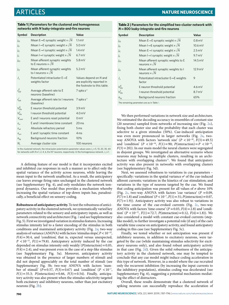
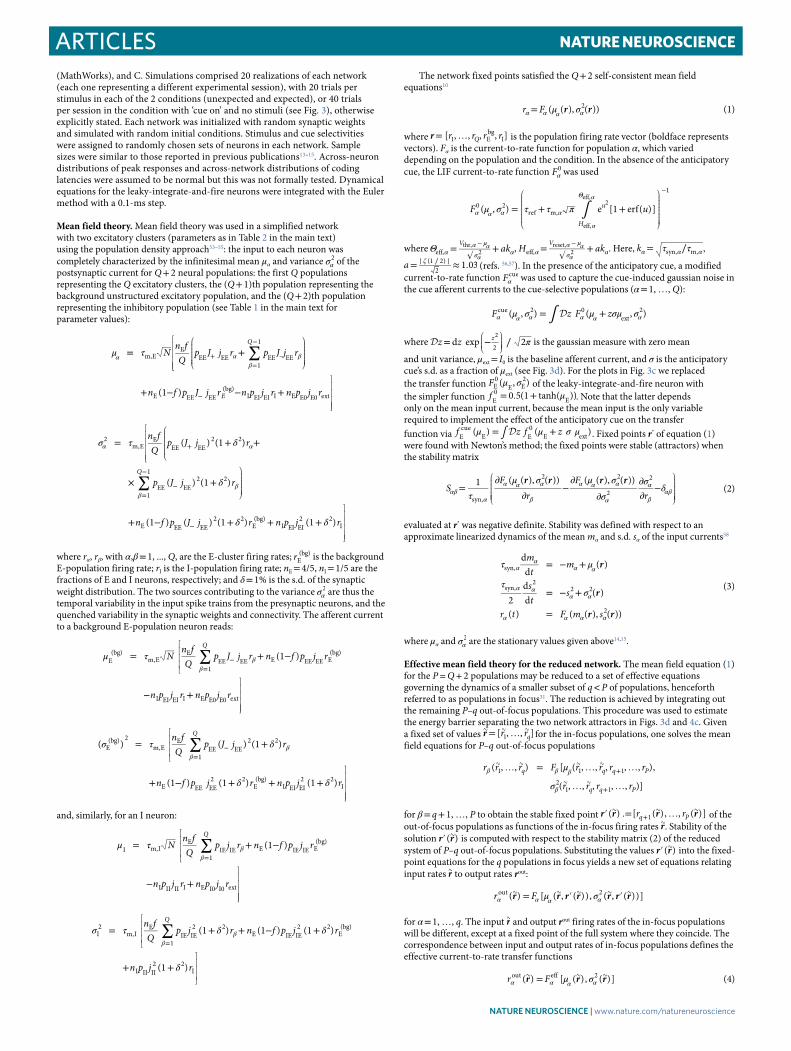
Fig. 2 | Robustness of anticipatory activity to variations in stimulus and cue models. a, Latency of significant decoding increased with stimulus intensity (left: top, stimulus peak expressed as percentage of baseline, darker shades represent stronger stimuli; bottom, decoding latency, mean ± s.e.m. across n = 20 simulated networks for each value on the x axis; see main text for a–c statistical tests) in both conditions, and it is faster in expected (pink) than in unexpected (blue) trials. Anticipatory activity was present for a large range of network sizes (right: J+ = 5, 10, 20, 30, 40 for N = 1, 2, 4, 6, 8 × 10³ neurons, respectively). Network synaptic weights scaled as reported in Tables 1 and 2. b, Anticipatory activity was present when stimuli targeted both excitatory (E) and inhibitory (I) neurons (notations as in Fig. 1c; 50% of both E and I neurons were targeted by the cue; inset: mean ± s.e.m. across n = 20 simulated networks, two-sided t-test, P = 0.0011). c, Increasing the cue-induced spatial variance in the afferent currents σ2 (top left: histogram of afferents’ peak values across neurons; x axis, expressed as percentage of baseline; y axis, calibration bar: 100 neurons) leads to more pronounced anticipatory activity (bottom left: latency in unexpected (blue) and expected (pink) trials). Anticipatory activity was present for a large range of cue time courses (top right: double exponential cue profile with rise and decay times [τ1,τ2] = g × [0.1,0.5] s, for g in the range from 1 to 3; bottom right: decoding latency during unexpected (blue) and unexpected (pink) trials). d, Anticipatory activity was also present when the cue targeted 50% of both E and I neurons (σ = 20% in baseline units; inset: mean ± s.e.m. across n = 20 simulated networks, two-sided t-test, P = 0.0034). a–d, *P < 0.05, **P < 0.01, ***P < 0.001, post hoc, multiple-comparison, two-sided t-test with Bonferroni correction. Horizontal black bar, P < 0.05, two-sided t-test with multiple-bin Bonferroni correction. Insets: **P < 0.01, ***P < 0.001, two-sided t-test. c,d, notations as in Fig. 1c.
NAtuRE NEuRosCiENCE | VOL 22 | MAY 2019 | 787–796 | www.nature.com/natureneuroscience 789
Articles NATuRe NeuROScIeNce
A defining feature of our model is that it incorporates excited and inhibited cue responses in such a manner as to affect only the spatial variance of the activity across neurons, while leaving the mean input to the network unaffected. As a result, the anticipatory cue leaves average firing rates unchanged in the clustered network (see Supplementary Fig. 4), and only modulates the network tem-poral dynamics. Our model thus provides a mechanism whereby increasing the spatial variance of top-down inputs has, paradoxi-cally, a beneficial effect on sensory coding.
Robustness of anticipatory activity. To test the robustness of antici-patory activity in the clustered network, we systematically varied key parameters related to the sensory and anticipatory inputs, as well as network connectivity and architecture (Fig. 2 and see Supplementary Fig. 5). First we investigated variation in stimulus features. Increasing stimulus intensity led to a faster encoding of the stimulus in both conditions and maintained anticipatory activity (Fig. 2a; two-way analysis of variance (ANOVA) with factors ‘stimulus slope’, P < 10−18, F(4) = 30.4, and ‘condition’, that is, expected versus unexpected, P < 10−15, F(1) = 79.8). Anticipatory activity induced by the cue depended on stimulus intensity only weakly (P(interaction) = 0.05, F(4) = 2.4), and was present even in the case of a step-like stimulus (see Supplementary Fig. 5a). Moreover, anticipatory activity was obtained in the presence of larger numbers of stimuli and did not depend appreciably on the total number of stimuli (see Supplementary Fig. 5b; two-way ANOVA with factors ‘num-ber of stimuli’ (P = 0.57, F(3) = 0.67) and ‘condition’ (P < 10−7, F(1) = 35.3; P(interaction) = 0.66, F(3) = 0.54). Finally, anticipa-tory activity was also present when the stimulus selectivity targeted both excitatory and inhibitory neurons, rather than just excitatory neurons (Fig. 2b).
We then performed variations in network size and architecture. We estimated the decoding accuracy in ensembles of constant size (20 neurons) sampled from networks of increasing size (Fig. 2a), fixing both cluster size and the probability that each cluster was selective to a given stimulus (50%). Cue-induced anticipation was even more pronounced in larger networks (Fig. 2a, two-way ANOVA with factors ‘network size’ (P < 10−20, F(3) = 49.5) and ‘condition’ (P < 10−16, F(1) = 90; P(interaction) = P < 10−10, F(3) = 20)). In our main model the neural clusters were segregated in disjoint groups. We investigated an alternative scenario where neurons may belong to multiple clusters, resulting in an archi-tecture with overlapping clusters30. We found that anticipatory activity was also present in networks with overlapping clusters (see Supplementary Fig. 5d).
Next, we assessed robustness to variations in cue parameters – specifically: variations in the spatial variance σ2 of the cue-induced afferent currents; variations in the kinetics of cue stimulation; and variations in the type of neurons targeted by the cue. We found that coding anticipation was present for all values of σ above 10% (Fig. 2c, two-way ANOVA with factors ‘cue variance’ (P = 0.09, F(7) = 1.8) and ‘condition’ (P < 10−7, F(1) = 31; P(interaction) = 0.07, F(7) = 1.9)). Anticipatory activity was also robust to variations in the time course of the cue-evoked currents (Fig. 2c, two-way ANOVA with factors ‘time course’ (P = 0.03, F(4) = 2.8) and ‘condi-tion’ (P < 10−15, F(1) = 72.7; P(interaction) = 0.12, F(4) = 1.8)). We also considered a model with constant cue-evoked currents (step-like model), to further investigate a potential role (if any) of the cue’s variable time course on anticipatory activity, and found anticipatory coding in this case (see Supplementary Fig. 5c).
Finally, we tested whether or not anticipation was present if inhibitory neurons, in addition to excitatory neurons, were tar-geted by the cue (while maintaining stimulus selectivity for excit-atory neurons only), and also found robust anticipatory activity in that case (Fig. 2d). Given the solid robustness of the anticipa-tory activity in the clustered network, one may be tempted to conclude that any cue model might induce coding acceleration in this type of network. However, in a model where the cue recruited only the recurrent inhibition (by increasing the input currents to the inhibitory population), stimulus coding was decelerated (see Supplementary Fig. 6), suggesting a potential mechanism mediat-ing the effect of distractors.
Overall, these results demonstrate that a clustered network of spiking neurons can successfully reproduce the acceleration of
Table 1 | Parameters for the clustered and homogeneous networks with N leaky-integrate-and-fire neurons
symbol Description Value
jEE Mean E→E synaptic weight × N 1.1 mV
jEI Mean I→E synaptic weight × N 5.0 mV
jIE Mean E→I synaptic weight × N 1.4 mV
jII Mean I→I synaptic weight × N 6.7 mV
jE0 Mean afferent synaptic weights to E neurons × N
5.8 mV
jI0 Mean afferent synaptic weights to I neurons × N
5.2 mV
J+ Potentiated intracluster E→E weights factor
Values depend on N and are explicitly reported in the footnote to this table.
rextE Average afferent rate to E
neurons (baseline)7 spks s–1
rextI Average afferent rate to I neurons
(baseline)7 spks s–1
VthrE E neuron threshold potential 3.9 mV
VthrI I neuron threshold potential 4.0 mV
Vreset E and I neurons reset potential 0 mV
τm E and I membrane time constant 20 ms
τref Absolute refractory period 5 ms
τsyn E and I synaptic time constant 4 ms
nbg Background neurons fraction 10%
Nc Average cluster size 100 neurons
In the clustered network, the intracluster potentiation parameter values were J+ = 5, 10, 20, 30, 40 for networks with N = 1, 2, 4, 6, 8 × 10³ neurons, respectively. In the homogeneous network, J+ = 1.
Table 2 | Parameters for the simplified two-cluster network with N = 800 leaky-integrate-and-fire neurons
symbol Description Value
jEE Mean E→E synaptic weight × N 0.8 mV
jEI Mean I→E synaptic weight × N 10.6 mV
jIE Mean E→I synaptic weight × N 2.5 mV
jII Mean I→I synaptic weight × N 9.7 mV
jE0 Mean afferent synaptic weights to E neurons × N
14.5 mV
jI0 Mean afferent synaptic weights to I neurons × N
12.9 mV
J+ Potentiated intracluster E→E weights factor
9
VthrE E neuron threshold potential 4.6 mV
VthrI I neuron threshold potential 8.7 mV
nbg Background neurons fraction 65%
The remaining parameters are as in Table 1.
NAtuRE NEuRosCiENCE | VOL 22 | MAY 2019 | 787–796 | www.nature.com/natureneuroscience790
ArticlesNATuRe NeuROScIeNce
sensory coding induced by expectation and that removing cluster-ing impairs this function.
Anticipatory cue speeds up the network’s dynamics. Having established that a clustered architecture enables the effects of expec-tation on coding, we investigated the underlying mechanism.
Clustered networks spontaneously generate highly structured activity characterized by coordinated patterns of ensemble firing. This activity results from the network hopping between metastable states in which different combinations of clusters are simultaneously activated11,13,14. To understand how anticipatory inputs affected net-work dynamics, we analyzed the effects of cue presentation for a prolonged period of 5 seconds in the absence of stimuli. Activating
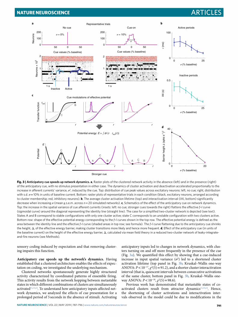
anticipatory inputs led to changes in network dynamics, with clus-ters turning on and off more frequently in the presence of the cue (Fig. 3a). We quantified this effect by showing that a cue-induced increase in input spatial variance (σ2) led to a shortened cluster activation lifetime (top panel in Fig. 3b; Kruskal–Wallis one-way ANOVA: P < 10−17, χ2(5) = 91.2), and a shorter cluster interactivation interval (that is, quiescent intervals between consecutive activations of the same cluster, bottom panel in Fig. 3b, Kruskal–Wallis one-way ANOVA: P < 10−18, χ2(5) = 98.6).
Previous work has demonstrated that metastable states of co-activated clusters result from attractor dynamics11,13,14. Hence, the shortening of cluster activations and interactivation inter-vals observed in the model could be due to modifications in the
σ = 10%σ = 0%
1 sActive
}}
Inactive
50 0 500
100
200
50 0 500
100
200
Cue values (% baseline)
Neu
rons
Neu
rons
× 1
03
No cue
σ
a
τ (m
s)IA
I (s)
Active periods
Inactive periods
0 250
0.5
0
100
b
1
2
d
σ (% baseline)
Cue values (% baseline)
Cue-onRepresentative trials
1
2
1 s
Stronger cue
r
rout
r r
r
E
r r
Tra
nsfe
r fu
nctio
nP
oten
tial
Potential energy: E = ∫ dr (r rout(r ))
c
BA BA BA
A
B
C
C
Δ
0 20
40
σ (% baseline)
Bar
rier
heig
ht Δ
(sp
ks s
–1)2
C
C
Cue modulations of effective potential
0 25
σ (% baseline)
0
Fig. 3 | Anticipatory cue speeds up network dynamics. a, Raster plots of the clustered network activity in the absence (left) and in the presence (right) of the anticipatory cue, with no stimulus presentation in either case. The dynamics of cluster activation and deactivation accelerated proportionally to the increase in afferent currents’ variance, σ2, induced by the cue. Top: distribution of cue peak values across excitatory neurons: left, no cue; right, distribution with s.d. σ = 10% in units of baseline current. Bottom: raster plots of representative trials in each condition (black, excitatory neurons, arranged according to cluster membership; red, inhibitory neurons). b, The average cluster activation lifetime (top) and interactivation interval (IAI, bottom) significantly decrease when increasing σ (mean ± s.e.m. across n = 20 simulated networks). c, Schematics of the effect of the anticipatory cue on network dynamics. Top: the increase in the spatial variance of cue afferent currents (insets: left: no cue; stronger cues towards the right) flattens the effective f–I curve (sigmoidal curve) around the diagonal representing the identity line (straight line). The case for a simplified two-cluster network is depicted (see text). States A and B correspond to stable configurations with only one cluster active; state C corresponds to an unstable configuration with two clusters active. Bottom row: shape of the effective potential energy corresponding to the f–I curves shown in the top row. The effective potential energy is defined as the area between the identity line and the effective f–I curve (shaded areas in top row; see formula). The f–I curve flattening due to the anticipatory cue shrinks the height, Δ, of the effective energy barrier, making cluster transitions more likely and hence more frequent. d, Effect of the anticipatory cue (in units of the baseline current) on the height of the effective energy barrier, Δ, calculated via mean field theory in a reduced two-cluster network of leaky-integrate-and-fire neurons (see Methods).
NAtuRE NEuRosCiENCE | VOL 22 | MAY 2019 | 787–796 | www.nature.com/natureneuroscience 791
Articles NATuRe NeuROScIeNce
network’s attractor dynamics. To test this hypothesis, we performed a mean field theory analysis30–33 of a simplified network with only two clusters, therefore producing a reduced repertoire of configura-tions. These include two configurations in which either cluster is active and the other inactive (A and B in Fig. 3c), and a configura-tion where both clusters are moderately active (C). The dynamics of this network can be analyzed using a reduced, self-consistent theory of a single excitatory cluster, said to be in focus31 (see Methods for details), based on the effective transfer function relating the input and output firing rates of the cluster (r and rout, Fig. 3c). The lat-ter are equal in the A, B, and C network configurations described above—also called ‘fixed points’ because these are the points where the transfer function intersects the identity line, rout = Φ(rin).
Configurations A and B would be stable in an infinitely large network, but they are only metastable in networks of finite size, due to intrinsically generated variability13. Transitions between metastable states can be modeled as a diffusion process and ana-lyzed using Kramers’ theory34, according to which the transi-tion rates depend on the height, Δ, of an effective energy barrier separating them13,34. In our theory, the effective energy barriers (see Fig. 3c, bottom row) are obtained as the area of the region between the identity line and the transfer function (shaded areas in top row of Fig. 3c; see Methods for details). The effective energy is constructed so that its local minima correspond to stable fixed points (here, A and B) whereas local maxima correspond to unsta-ble fixed points (C). Larger barriers correspond to less frequent transitions between stable configurations, whereas lower barriers
increase the transition rates and therefore accelerate the network’s metastable dynamics.
This picture provides the substrate for understanding the role of the anticipatory cue in the expectation effect. Basically, the pre-sentation of the cue modulates the shape of the effective transfer function, which results in the reduction of the effective energy bar-riers. More specifically, the cue-induced increase in the spatial vari-ance, σ2, of the afferent current, flattens the transfer function along the identity line, reducing the area between the two curves (shaded regions in Fig. 3c). In turn, this reduces the effective energy barrier separating the two configurations (Fig. 3c, bottom row), resulting in faster dynamics. The larger the cue-induced spatial variance σ2 in the afferent currents, the faster the dynamics (Fig. 3d; lighter shades represent larger σ values).
In summary, this analysis shows that the anticipatory cue increases the spontaneous transition rates between the network’s metastable configurations by reducing the effective energy bar-rier necessary to hop among configurations. In the following we uncover an important consequence of this phenomenon for sen-sory processing.
Anticipatory cue induces faster onset of taste-coding states. The cue-induced modulation of attractor dynamics led us to formu-late a hypothesis for the mechanism underlying the acceleration of coding: the activation of anticipatory inputs before sensory stimu-lation may allow the network to enter stimulus-coding configura-tions more easily while exiting non-coding configurations more
0 1–1 0 1–1
Clusteractivation
40 (
spks
s–1
)2
0
90
ΔNC→C
ΔC→NC
Stimulus intensity (%)
0 5
Δ (s
pks
s–1)2
Expected Unexpected
Time (s) Time (s)
4
8
12
16
4
8
12
16
Exc
itato
ry n
euro
ns ×
102
Exc
itato
ry n
euro
ns ×
102
Stimulus StimulusCue
a
b c
Distance along trajectory
Cue OFF
Cue ON
Cue OFFCue ON
Stronger stim
ulus
Pot
entia
l
Codingstate
Non-codingstate
Stimulus-selectiveNon-selective
0
0.4 ***
Late
ncy
(s)
Exp
ecte
d
Une
xpec
ted
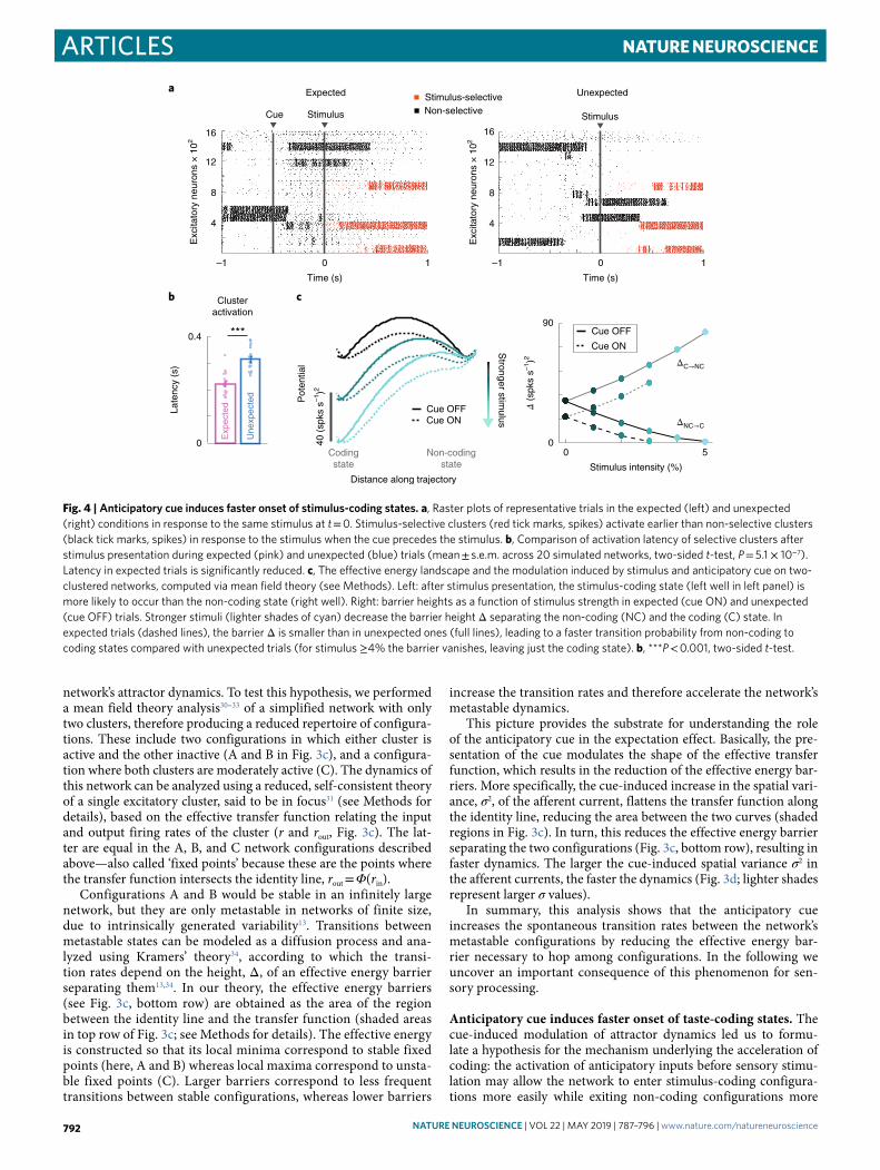
Fig. 4 | Anticipatory cue induces faster onset of stimulus-coding states. a, Raster plots of representative trials in the expected (left) and unexpected (right) conditions in response to the same stimulus at t = 0. Stimulus-selective clusters (red tick marks, spikes) activate earlier than non-selective clusters (black tick marks, spikes) in response to the stimulus when the cue precedes the stimulus. b, Comparison of activation latency of selective clusters after stimulus presentation during expected (pink) and unexpected (blue) trials (mean ± s.e.m. across 20 simulated networks, two-sided t-test, P = 5.1 × 10⁻⁷). Latency in expected trials is significantly reduced. c, The effective energy landscape and the modulation induced by stimulus and anticipatory cue on two-clustered networks, computed via mean field theory (see Methods). Left: after stimulus presentation, the stimulus-coding state (left well in left panel) is more likely to occur than the non-coding state (right well). Right: barrier heights as a function of stimulus strength in expected (cue ON) and unexpected (cue OFF) trials. Stronger stimuli (lighter shades of cyan) decrease the barrier height Δ separating the non-coding (NC) and the coding (C) state. In expected trials (dashed lines), the barrier Δ is smaller than in unexpected ones (full lines), leading to a faster transition probability from non-coding to coding states compared with unexpected trials (for stimulus ≥4% the barrier vanishes, leaving just the coding state). b, ***P < 0.001, two-sided t-test.
NAtuRE NEuRosCiENCE | VOL 22 | MAY 2019 | 787–796 | www.nature.com/natureneuroscience792
ArticlesNATuRe NeuROScIeNce
easily. Figure 4a shows simulated population rasters in response to the same stimulus presented in the absence of, or following, a cue. Spikes in red represent activity in taste-selective clusters and show a faster activation latency in response to the stimulus preceded by the cue compared with the uncued condition. A systematic analysis revealed that, in the cued condition, the clusters activated by the subsequent stimulus had a significantly faster activation latency than in the uncued condition (Fig. 4b, 0.22 ± 0.01 s (mean ± s.e.m.) during cued compared with 0.32 ± 0.01 s for uncued stimuli; P < 10−5, two-sided t-test, degrees of freedom = 39).
We explained this effect using mean field theory. In the simpli-fied two-cluster network of Fig. 4c (the same network as in Fig. 3d), the configuration where the taste-selective cluster is active (cod-ing state) or the non-selective cluster is active (non-coding state) have initially the same effective potential energy (local minima of the black line in Fig. 4c). The onset of the cue reduces the effec-tive energy barrier separating these configurations (dashed versus full line). After stimulus onset, the coding state sits in a deeper well (lighter lines) compared with the non-coding state, due to the stimulation biasing the selective cluster. Stronger stimuli (lighter shades in Fig. 4c) progressively increase the difference between the wells’ depths breaking their initial symmetry, making a transition from the non-coding to the coding state more likely than a transi-tion from the coding to the non-coding state34. The anticipatory cue reduces further the existing barrier and thereby increases the transi-tion rate toward coding configurations. This results in faster coding, on average, of the encoded stimuli.
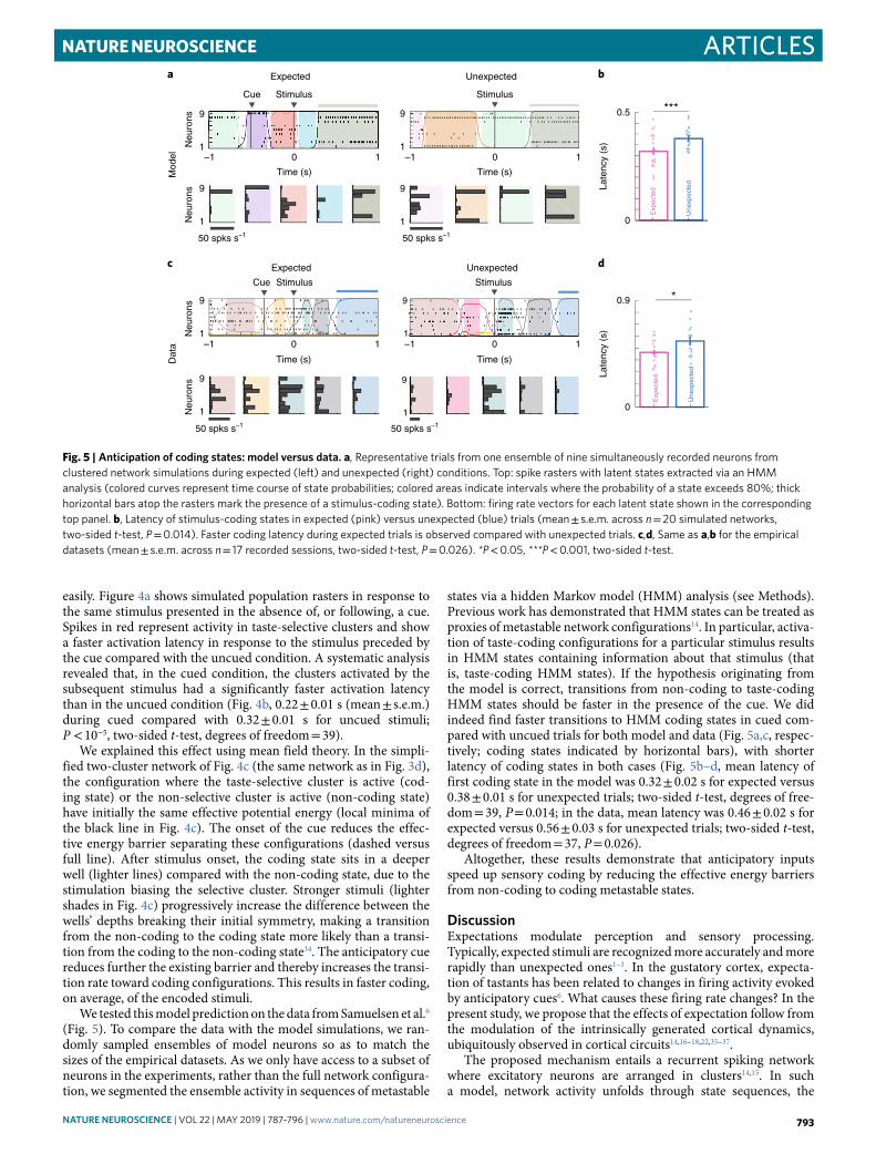
We tested this model prediction on the data from Samuelsen et al.6 (Fig. 5). To compare the data with the model simulations, we ran-domly sampled ensembles of model neurons so as to match the sizes of the empirical datasets. As we only have access to a subset of neurons in the experiments, rather than the full network configura-tion, we segmented the ensemble activity in sequences of metastable
states via a hidden Markov model (HMM) analysis (see Methods). Previous work has demonstrated that HMM states can be treated as proxies of metastable network configurations14. In particular, activa-tion of taste-coding configurations for a particular stimulus results in HMM states containing information about that stimulus (that is, taste-coding HMM states). If the hypothesis originating from the model is correct, transitions from non-coding to taste-coding HMM states should be faster in the presence of the cue. We did indeed find faster transitions to HMM coding states in cued com-pared with uncued trials for both model and data (Fig. 5a,c, respec-tively; coding states indicated by horizontal bars), with shorter latency of coding states in both cases (Fig. 5b–d, mean latency of first coding state in the model was 0.32 ± 0.02 s for expected versus 0.38 ± 0.01 s for unexpected trials; two-sided t-test, degrees of free-dom = 39, P = 0.014; in the data, mean latency was 0.46 ± 0.02 s for expected versus 0.56 ± 0.03 s for unexpected trials; two-sided t-test, degrees of freedom = 37, P = 0.026).
Altogether, these results demonstrate that anticipatory inputs speed up sensory coding by reducing the effective energy barriers from non-coding to coding metastable states.
DiscussionExpectations modulate perception and sensory processing. Typically, expected stimuli are recognized more accurately and more rapidly than unexpected ones1–3. In the gustatory cortex, expecta-tion of tastants has been related to changes in firing activity evoked by anticipatory cues6. What causes these firing rate changes? In the present study, we propose that the effects of expectation follow from the modulation of the intrinsically generated cortical dynamics, ubiquitously observed in cortical circuits14,16–18,22,35–37.
The proposed mechanism entails a recurrent spiking network where excitatory neurons are arranged in clusters14,15. In such a model, network activity unfolds through state sequences, the
Late
ncy
(s)
Late
ncy
(s)
***
*
Neu
rons
Neu
rons
1
9
1
9
Dat
a
StimulusStimulusCue
0 1–1 0 1–1
1
9
UnexpectedExpecteda b
c d
Neu
rons
Neu
rons
Mod
el 0 1–1
Time (s) Time (s)
Time (s) Time (s)
0 1–1
1
9
50 spks s–1
50 spks s–1 50 spks s–1
50 spks s–1
1
9
Stimulus
1
9
StimulusCue
0
0.9
0
0.5
Exp
ecte
d
Une
xpec
ted
Exp
ecte
d
Une
xpec
ted
UnexpectedExpected
1
9
1
9
Fig. 5 | Anticipation of coding states: model versus data. a, Representative trials from one ensemble of nine simultaneously recorded neurons from clustered network simulations during expected (left) and unexpected (right) conditions. Top: spike rasters with latent states extracted via an HMM analysis (colored curves represent time course of state probabilities; colored areas indicate intervals where the probability of a state exceeds 80%; thick horizontal bars atop the rasters mark the presence of a stimulus-coding state). Bottom: firing rate vectors for each latent state shown in the corresponding top panel. b, Latency of stimulus-coding states in expected (pink) versus unexpected (blue) trials (mean ± s.e.m. across n = 20 simulated networks, two-sided t-test, P = 0.014). Faster coding latency during expected trials is observed compared with unexpected trials. c,d, Same as a,b for the empirical datasets (mean ± s.e.m. across n = 17 recorded sessions, two-sided t-test, P = 0.026). *P < 0.05, ***P < 0.001, two-sided t-test.
NAtuRE NEuRosCiENCE | VOL 22 | MAY 2019 | 787–796 | www.nature.com/natureneuroscience 793
Articles NATuRe NeuROScIeNce
dynamics of which speed up in the presence of an anticipatory cue. This anticipates the onset of ‘coding states’ (containing the most information about the delivered stimulus), and explains the faster decoding latency observed by Samuelsen et al.6 (see Fig. 1c).
Notably, this anticipatory mechanism is unrelated to changes in network excitability, which would lead to unidirectional changes in firing rates. It relies instead on an increase in the spatial (that is, across neurons) variance of the network’s activity caused by the anticipatory cue. This increase in the input’s variance is observed experimentally after training9, and is therefore the consequence of having learned the anticipatory meaning of the cue. The consequent acceleration of state sequences predicted by the model was also con-firmed in the data from ensembles of simultaneously recorded neu-rons in awake-behaving rats.
These results provide a functional interpretation of ongoing cor-tical activity and a precise explanatory link between the intrinsic dynamics of neural activity in a sensory circuit and a specific cogni-tive process, that of general expectation6,38.
Clustered connectivity and metastable states. A key feature of our model is the clustered architecture of the excitatory population. Theoretical work had previously shown that a clustered architecture can produce stable activity patterns10. Noise (either externally11,39 or internally13,14 generated) may destabilize those patterns and ignite a progression through metastable states. These states are reminiscent of those observed in the cortex during both task engagement12,16,40,41 and inter-trial periods14,36, including those found in rodent gustatory cortex during taste processing and decision-making14,39,42. Clustered spiking networks also account for various physiological observa-tions such as stimulus-induced reduction of trial-to-trial variabil-ity11,13,14,43, neural dimensionality15, and firing rate multistability14.
In the present study, we showed that clustered spiking networks also have the ability to modulate coding latency and therefore explain the phenomenon of general expectation. The uncovered link of generic anticipatory cues, network metastability, and coding speed is dependent on a clustered architecture, because removing the excitatory clusters (that is, having homogeneous connectivity) eliminates the anticipatory mechanism (see Fig. 1d–f).
Functional role of heterogeneity in cue responses. As stated in the previous section, the presence of clusters is a necessary ingredient to obtain a faster latency of coding. Below we discuss the second necessary ingredient, that is, the presence of heterogeneous neural responses to the anticipatory cue (see Fig. 1b).
Responses to anticipatory cues have been extensively studied in cortical and subcortical areas in alert rodents6,9,44,45. Cues evoke het-erogeneous patterns of activity, either exciting or inhibiting single neurons. The proportion of cue responses and their heterogene-ity develop with training9,45, suggesting a fundamental function of these patterns. In the generic expectation paradigm considered here, the anticipatory cue does not convey any information about the identity of the forthcoming tastant, but rather it just signals the availability of a stimulus. Experimental evidence suggests that the cue may induce a state of arousal, which was previously described as ‘priming’ the sensory cortex6,46. Here, we propose an underly-ing mechanism in which the cue is responsible for acceleration of coding by increasing the spatial variance of the pre-stimulus activ-ity. In turn, this modulates the shape of the neuronal current-to-rate transfer function and thus lowers the effective energy barriers between metastable configurations.
We note that the presence of both excited and inhibited cue responses poses a challenge to simple models of neuromodulation. The presence of cue-evoked suppression of firing9 suggests that cues do not improve coding by simply increasing the excitability of corti-cal areas. Additional mechanisms and complex patterns of connec-tivity may be required to explain the suppression effects induced by
the cue. However, in the present study we provide a parsimonious explanation of how heterogeneous responses can improve coding without postulating any specific pattern of connectivity other than (1) random projections from thalamic and anticipatory cue affer-ents and (2) the clustered organization of the intracortical circuitry. Notice that the latter contains wide distributions of synaptic weights and can be understood as the consequence of Hebb-like reorganiza-tion of the circuitry during training47,48.
Specificity of the anticipatory mechanism. Our model of antici-pation relies on gain reduction in clustered excitatory neurons due to a larger spatial variance of the afferent currents. We have shown that this model is robust to variations in parameters and architec-ture (see Fig. 2 and Supplementary Fig. 5); what about the speci-ficity of its mechanism? A priori, the expectation effect might be achieved through different means, such as: increasing the strength of feedforward couplings; decreasing the strength of recurrent cou-plings; or modulating background synaptic inputs49. However, when scoring those models on the criteria of coding anticipation and het-erogeneous cue responses, we found that they failed to simultane-ously match both criteria, although for some range of parameters they could reproduce either one (see Supplementary Figs. 7–9 and Supplementary Table 1 for a detailed analysis).
Although our exploration of the alternative models’ parameter space did not produce an example that could match the data, we cannot in principle exclude the possibility that one of the alterna-tive models could match the data in a yet unexplored parameter region. This may be particularly the case for the model shown in Supplementary Fig. 7c, which can produce anticipation of coding but does not match the patterns of cue responses observed in the experiments. We are aware that, due to the typically large number of cellular and network parameters, it is hard to rule out these or other alternative models entirely. We could, however, demonstrate that the main mechanism proposed here (see Fig. 1a) captures the plurality of experimental observations pertaining to anticipatory activity in a robust and biologically plausible way.
Cortical timescales, state transitions, and cognitive function. In populations of spiking neurons, a clustered architecture can generate reverberating activity and sequences of metastable states. Transitions from state to state can be typically caused by external inputs13,14. For instance, in frontal cortices, sequences of states are related to specific epochs within a task, with transitions evoked by behavioral events16,17,20. In sensory cortex, progressions through state sequences can be triggered by sensory stimuli and reflect the dynamics of sensory processing21,40. Importantly, state sequences have also been observed in the absence of any external stimulation, promoted by intrinsic fluctuations in neural activity14,37. However, the potential functional role, if any, of this type of ongoing activity has remained unexplored.
Recent work has started to uncover the link between ensemble dynamics and sensory and cognitive processes. State transitions in various cortical areas have been linked to decision-making39,50, choice representation20, rule-switching behavior22, and the level of task difficulty21. However, no theoretical or mechanistic explana-tions have been given for these phenomena.
Here we provide a mechanistic link between state sequences and expectation in terms of specific modulations of intrinsic dynamics, that is, the anticipatory cue triggers a change of the transition prob-abilities. The modulation of intrinsic activity can dial the duration of states, producing either shorter or longer timescales. A shorter timescale leads to faster state sequences and coding anticipation after stimulus presentation (see Figs. 1 and 5). Other external per-turbations may induce different effects: for example, recruiting the network’s inhibitory population slows down the timescale, leading to a slower coding (see Supplementary Fig. 6).
NAtuRE NEuRosCiENCE | VOL 22 | MAY 2019 | 787–796 | www.nature.com/natureneuroscience794

ArticlesNATuRe NeuROScIeNce
The interplay between intrinsic dynamics and anticipatory influences presented here is a mechanism for generating diverse timescales, and may have rich computational consequences. We demonstrated its function in increasing coding speed, but its role in mediating cognition is likely to be broader and calls for further explorations.
online contentAny methods, additional references, Nature Research reporting summaries, source data, statements of data availability and asso-ciated accession codes are available at https://doi.org/10.1038/s41593-019-0364-9.
Received: 6 October 2017; Accepted: 15 February 2019; Published online: 1 April 2019
References 1. Gilbert, C. D. & Sigman, M. Brain states: top-down influences in sensory
processing. Neuron 54, 677–696 (2007). 2. Jaramillo, S. & Zador, A. M. The auditory cortex mediates the
perceptual effects of acoustic temporal expectation. Nat. Neurosci. 14, 246–251 (2011).
3. Engel, A. K., Fries, P. & Singer, W. Dynamic predictions: oscillations and synchrony in top-down processing. Nat. Rev. Neurosci. 2, 704–716 (2001).
4. Doherty, J. R., Rao, A., Mesulam, M. M. & Nobre, A. C. Synergistic effect of combined temporal and spatial expectations on visual attention. J. Neurosci. 25, 8259–8266 (2005).
5. Niwa, M., Johnson, J. S., O’Connor, K. N. & Sutter, M. L. Active engagement improves primary auditory cortical neurons’ ability to discriminate temporal modulation. J. Neurosci. 32, 9323–9334 (2012).
6. Samuelsen, C. L., Gardner, M. P. & Fontanini, A. Effects of cue-triggered expectation on cortical processing of taste. Neuron 74, 410–422 (2012).
7. Yoshida, T. & Katz, D. B. Control of prestimulus activity related to improved sensory coding within a discrimination task. J. Neurosci. 31, 4101–4112 (2011).
8. Gardner, M. P. & Fontanini, A. Encoding and tracking of outcome- specific expectancy in the gustatory cortex of alert rats. J. Neurosci. 34, 13000–13017 (2014).
9. Vincis, R. & Fontanini, A. Associative learning changes cross-modal representations in the gustatory cortex. eLife 5, e16420 (2016).
10. Amit, D. J. & Brunel, N. Model of global spontaneous activity and local structured activity during delay periods in the cerebral cortex. Cereb. Cortex 7, 237–252 (1997).
11. Deco, G. & Hugues, E. Neural network mechanisms underlying stimulus driven variability reduction. PLoS Comput. Biol. 8, e1002395 (2012).
12. Harvey, C. D., Coen, P. & Tank, D. W. Choice-specific sequences in parietal cortex during a virtual-navigation decision task. Nature 484, 62–68 (2012).
13. Litwin-Kumar, A. & Doiron, B. Slow dynamics and high variability in balanced cortical networks with clustered connections. Nat. Neurosci. 15, 1498–1505 (2012).
14. Mazzucato, L., Fontanini, A. & La Camera, G. Dynamics of multistable states during ongoing and evoked cortical activity. J. Neurosci. 35, 8214–8231 (2015).
15. Mazzucato, L., Fontanini, A. & La Camera, G. Stimuli reduce the dimensionality of cortical activity. Front. Syst. Neurosci. 10, 11 (2016).
16. Abeles, M. et al. Cortical activity flips among quasi-stationary states. Proc. Natl Acad. Sci. USA 92, 8616–8620 (1995).
17. Seidemann, E., Meilijson, I., Abeles, M., Bergman, H. & Vaadia, E. Simultaneously recorded single units in the frontal cortex go through sequences of discrete and stable states in monkeys performing a delayed localization task. J. Neurosci. 16, 752–768 (1996).
18. Arieli, A., Shoham, D., Hildesheim, R. & Grinvald, A. Coherent spatiotemporal patterns of ongoing activity revealed by real-time optical imaging coupled with single-unit recording in the cat visual cortex. J. Neurophysiol. 73, 2072–2093 (1995).
19. Arieli, A., Sterkin, A., Grinvald, A. & Aertsen, A. Dynamics of ongoing activity: explanation of the large variability in evoked cortical responses. Science 273, 1868–1871 (1996).
20. Rich, E. L. & Wallis, J. D. Decoding subjective decisions from orbitofrontal cortex. Nat. Neurosci. 19, 973–980 (2016).
21. Ponce-Alvarez, A., Nácher, V., Luna, R., Riehle, A. & Romo, R. Dynamics of cortical neuronal ensembles transit from decision making to storage for later report. J. Neurosci. 32, 11956–11969 (2012).
22. Durstewitz, D., Vittoz, N. M., Floresco, S. B. & Seamans, J. K. Abrupt transitions between prefrontal neural ensemble states accompany behavioral transitions during rule learning. Neuron 66, 438–448 (2010).
23. Renart, A. et al. The asynchronous state in cortical circuits. Science 327, 587–590 (2010).
24. Chen, X., Gabitto, M., Peng, Y., Ryba, N. J. & Zuker, C. S. A gustotopic map of taste qualities in the mammalian brain. Science 333, 1262–1266 (2011).
25. Fletcher, M. L., Ogg, M. C., Lu, L., Ogg, R. J. & Boughter, J. D. Jr. Overlapping Representation of primary tastes in a defined region of the gustatory cortex. J. Neurosci. 37, 7595–7605 (2017).
26. Kiani, R. et al. Natural grouping of neural responses reveals spatially segregated clusters in prearcuate cortex. Neuron 85, 1359–1373 (2015).
27. Katz, D. B., Simon, S. A. & Nicolelis, M. A. Dynamic and multimodal responses of gustatory cortical neurons in awake rats. J. Neurosci. 21, 4478–4489 (2001).
28. Jezzini, A., Mazzucato, L., La Camera, G. & Fontanini, A. Processing of hedonic and chemosensory features of taste in medial prefrontal and insular networks. J. Neurosci. 33, 18966–18978 (2013).
29. van Vreeswijk, C. & Sompolinsky, H. Chaos in neuronal networks with balanced excitatory and inhibitory activity. Science 274, 1724–1726 (1996).
30. Curti, E., Mongillo, G., La Camera, G. & Amit, D. J. Mean field and capacity in realistic networks of spiking neurons storing sparsely coded random memories. Neural Comput. 16, 2597–2637 (2004).
31. Mascaro, M. & Amit, D. J. Effective neural response function for collective population states. Network 10, 351–373 (1999).
32. Mattia, M. et al. Heterogeneous attractor cell assemblies for motor planning in premotor cortex. J. Neurosci. 33, 11155–11168 (2013).
33. La Camera, G., Giugliano, M., Senn, W. & Fusi, S. The response of cortical neurons to in vivo-like input current: theory and experiment: I. Noisy inputs with stationary statistics. Biol. Cybern. 99, 279–301 (2008).
34. Hänggi, P., Talkner, P. & Borkovec, M. Reaction-rate theory: Fifty years after Kramers. Rev. Mod. Phys. 62, 251 (1990).
35. Kenet, T., Bibitchkov, D., Tsodyks, M., Grinvald, A. & Arieli, A. Spontaneously emerging cortical representations of visual attributes. Nature 425, 954–956 (2003).
36. Pastalkova, E., Itskov, V., Amarasingham, A. & Buzsáki, G. Internally generated cell assembly sequences in the rat hippocampus. Science 321, 1322–1327 (2008).
37. Luczak, A., Barthó, P. & Harris, K. D. Spontaneous events outline the realm of possible sensory responses in neocortical populations. Neuron 62, 413–425 (2009).
38. Puccini, G. D., Sanchez-Vives, M. V. & Compte, A. Integrated mechanisms of anticipation and rate-of-change computations in cortical circuits. PLoS Comput. Biol. 3, e82 (2007).
39. Miller, P. & Katz, D. B. Stochastic transitions between neural states in taste processing and decision-making. J. Neurosci. 30, 2559–2570 (2010).
40. Jones, L. M., Fontanini, A., Sadacca, B. F., Miller, P. & Katz, D. B. Natural stimuli evoke dynamic sequences of states in sensory cortical ensembles. Proc. Natl. Acad. Sci. USA 104, 18772–18777 (2007).
41. Runyan, C. A., Piasini, E., Panzeri, S. & Harvey, C. D. Distinct timescales of population coding across cortex. Nature 548, 92–96 (2017).
42. Sadacca, B. F. et al. The behavioral relevance of cortical neural ensemble responses emerges suddenly. J. Neurosci. 36, 655–669 (2016).
43. Churchland, M. M. et al. Stimulus onset quenches neural variability: A widespread cortical phenomenon. Nat. Neurosci. 13, 369–378 (2010).
44. Liu, H. & Fontanini, A. State dependency of chemosensory coding in the gustatory thalamus (VPMpc) of alert rats. J. Neurosci. 35, 15479–15491 (2015).
45. Grewe, B. F. et al. Neural ensemble dynamics underlying a long-term associative memory. Nature 543, 670–675 (2017).
46. Chow, S. S., Romo, R. & Brody, C. D. Context-dependent modulation of functional connectivity: secondary somatosensory cortex to prefrontal cortex connections in two-stimulus-interval discrimination tasks. J. Neurosci. 29, 7238–7245 (2009).
47. Zenke, F., Agnes, E. J. & Gerstner, W. Diverse synaptic plasticity mechanisms orchestrated to form and retrieve memories in spiking neural networks. Nat. Commun. 6, 6922 (2015).
48. Litwin-Kumar, A. & Doiron, B. Formation and maintenance of neuronal assemblies through synaptic plasticity. Nat. Commun. 5, 5319 (2014).
49. Chance, F. S., Abbott, L. F. & Reyes, A. D. Gain modulation from background synaptic input. Neuron 35, 773–782 (2002).
50. Engel, T. A. et al. Selective modulation of cortical state during spatial attention. Science 354, 1140–1144 (2016).
AcknowledgementsThis work was supported by a National Institute of Deafness and Other Communication Disorders Grant no. K25-DC013557 (L.M.), by the Swartz Foundation Award 66438 (L.M.), by National Institute of Deafness and Other Communication Disorders
NAtuRE NEuRosCiENCE | VOL 22 | MAY 2019 | 787–796 | www.nature.com/natureneuroscience 795

Articles NATuRe NeuROScIeNce
Grant nos. R01DC012543 and R01DC015234 (A.F.), and partly by a National Science Foundation Grant no. IIS1161852 (G.L.C.). The authors would like to thank S. Fusi, A. Maffei, G. Mongillo, and C. van Vreeswijk for useful discussions.
Author contributionsL.M., G.L.C., and A.F. designed the project, discussed the models and the data analyses, and wrote the manuscript. L.M. performed the data analysis, model simulations, and theoretical analyses.
Competing interestsThe authors declare no competing interests.
Additional informationSupplementary information is available for this paper at https://doi.org/10.1038/s41593-019-0364-9.
Reprints and permissions information is available at www.nature.com/reprints.
Correspondence and requests for materials should be addressed to G.C. or A.F.
Journal peer review information: Nature Neuroscience thanks Paul Miller and other anonymous reviewer(s) for their contribution to the peer review of this work.
Publisher’s note: Springer Nature remains neutral with regard to jurisdictional claims in published maps and institutional affiliations.
© The Author(s), under exclusive licence to Springer Nature America, Inc. 2019
NAtuRE NEuRosCiENCE | VOL 22 | MAY 2019 | 787–796 | www.nature.com/natureneuroscience796
ArticlesNATuRe NeuROScIeNce
MethodsBehavioral training and electrophysiology. The experimental data come from a previously published dataset6. Experimental procedures were approved by the Institutional Animal Care and Use Committee of Stony Brook University and complied with university, state, and federal regulations on the care and use of laboratory animals. Movable bundles of 16 microwires were implanted bilaterally in the gustatory cortex and intraoral cannulae were inserted bilaterally. After postsurgical recovery, rats were trained to self-administer fluids through intraoral cannulae by pressing a lever under head-restraint within 3 s presentation of an auditory cue (expected trials; a 75-dB pure tone at a frequency of 5 kHz). The intertrial interval was progressively increased to 40 ± 3 s. Early presses were discouraged by the addition of a 2-s delay to the intertrial interval. During training and electrophysiology sessions, additional tastants were automatically delivered through the intraoral cannulae at random times near the middle of the intertrial interval and in the absence of the anticipatory cue (unexpected trials). The following tastants were delivered: 100 mmol l–1 NaCl, 100 mmol l–1 sucrose, 100 mmol l–1 citric acid, and 1 mmol l–1 quinine HCl. Water (50 μl) was delivered to rinse the mouth clean through a second intraoral cannula, 5 s after the delivery of each tastant. Multiple single-unit action potentials were amplified, bandpass filtered, and digitally recorded. Single units were isolated using a template algorithm, clustering techniques, and examination of interspike interval plots (Offline Sorter, Plexon). Starting from a pool of 299 single neurons in 37 sessions, neurons with peak firing rate lower than 1 spikes s–1 (defined as silent) were excluded from further analysis, as well as neurons with a large peak around the 6–10 Hz in the spike power spectrum, which were classified as somatosensory27,28. Only ensembles with five or more simultaneously recorded neurons were included in the rest of the analyses. Ongoing and evoked activity were defined as occurring in the 5-s-long interval before or after taste delivery, respectively.
Cue responsiveness. A neuron was deemed responsive to the cue if a sudden change in its firing rate was observed during the post-cue interval, detected via a ‘change-point’ procedure described in the literature28. Briefly, we built the cumulative distribution function of the spike count (CumSC) across all trials in each session, in the interval starting 0.5 s before, and ending 1 s after, cue delivery. We then ran the change-point detection algorithm on the CumSC record with a given tolerance level P = 0.05. If any change point was detected before cue presentation, the algorithm was repeated with lower tolerance (lower P value) until no change point was present before the cue. If a legitimate change point was found anywhere within 1 s after cue presentation, the neuron was deemed responsive. If no change point was found, the neuron was deemed not responsive. For neurons with excited (inhibited) cue responses, change in peristimulus time histogram (ΔPSTH) was defined as the difference between positive (negative) peak responses post-cue and the mean baseline activity in the 0.5 s preceding cue presentation.
Ensemble states detection. An HMM analysis was used to detect ensemble states in both the empirical data and the model simulations. Below, we give a brief description of the method used and we refer the reader the literature14,16,21,40 for more detailed information.
The HMM assumes that an ensemble of N simultaneously recorded neurons is in one of M hidden states at each given time bin. States are firing rate vectors ri(m), where i = 1, …, N is the neuron index and m = 1, …, M identifies the state. In each state, neurons were assumed to discharge as stationary Poisson processes (Poisson-HMM) conditional on the state’s firing rates. Trials were segmented in 2-ms bins, and the value of either 1 (spike) or 0 (no spike) was assigned to each bin for each given neuron (Bernoulli approximation for short time bins); if more than one neuron fired in a given bin (a rare event), a single spike was randomly assigned to one of the firing neurons. A single HMM was used to fit all trials in each recording session, resulting in the emission probabilities ri(m) and in a set of transition probabilities between the states. Emission and transition probabilities were calculated using the Baum–Welch algorithm51 with a fixed number of hidden states M, yielding a maximum likelihood estimate of the parameters given the observed spike trains. As the model log-likelihood, LL, increases with M, we repeated the HMM fits for increasing values of M until we hit a minimum of the Bayesian information criterion (BIC, see below and Zucchini and MacDonald51). For each M, the LL used in the BIC was the sum of over ten independent HMM fits with random initial guesses for emission and transition probabilities. This step was needed because the Baum–Welch algorithm guarantees reaching only a local rather than a global maximum of the likelihood. The model with the lowest BIC (having M* states) was selected as the winning model, where
= − + − +M M MN TBIC 2LL [ ( 1) ]ln , T being the number of observations in each session (which equals number of trials × number of bins per trials). Finally, the winning HMM model was used to ‘decode’ the states from the data according to their posterior probability, given the data. During decoding, only those states with probability exceeding 80% in at least 25 consecutive 2-ms bins were retained (henceforth denoted simply as states)15,40. This procedure eliminates states that appear only very transiently and with low probability, also reducing the chance of overfitting. A median of six states per ensemble was found, varying from three to nine across ensembles.
Coding states. In each condition (that is, expected versus unexpected), the frequencies of occurrence of a given state across taste stimuli were compared with a test of proportions (χ2, P < 0.001 with Bonferroni correction to account for multiple states). When a significant difference was found across stimuli, a post-hoc Marascuilo test was performed52. A state with a frequency of occurrence significantly higher in the presence of one taste stimulus compared with all other tastes was deemed a ‘coding state’ for that stimulus (see Fig. 5).
Spiking network model. We modeled the local neural circuit as a recurrent network of N leaky-integrate-and-fire neurons, with a fraction nE = 80% of excitatory (E) and nI = 20% of inhibitory (I) neurons10. Connectivity was random with probability pEE = 0.2 for E-to-E connections and pEI = pIE = pII = 0.5 otherwise. Synaptic weights Jij from presynaptic neuron j ∈ E,I to postsynaptic neuron i ∈ E,I scaled as = ∕J j Nij ij , with jij drawn from normal distributions and mean jαβ (for α,β = E,I) and 1% s.d. Networks of different architectures were considered: (1) networks with segregated clusters (referred to as clustered network, parameters as in Tables 1 and 2 in the main text); (2) networks with overlapping clusters (see Supplementary Fig. 5d and Supplementary Table 2 for details); and (3) homogeneous networks (parameters as in Table 1 in the main text). In the clustered network, E neurons were arranged in Q clusters with Nc = 100 neurons per cluster on average (1% s.d.), the remaining fraction nbg of E neurons belonging to an unstructured background population. In the clustered network, neurons belonging to the same cluster had intracluster synaptic weights potentiated by a factor J+; synaptic weights between neurons belonging to different clusters were depressed by a factor J− = 1 − f(J+ − 1)/2 < 1 with γ = 0.5; f = (1 − nbg)/Q is the average number of neurons in each cluster10. When changing the network size N, all synaptic weights Jij were scaled by N , the intracluster potentiation values were J+ = 5, 10, 20, 30, 40 for N = 1, 2, 4, 6, 8 × 10³ neurons, respectively, and cluster size remained unchanged (see also Table 1); all other parameters were kept fixed. In the homogeneous network, there were no clusters (J+ = J− = 1).
Model neuron dynamics. Below threshold the leaky-integrate-and-fire neuron membrane potential evolved in time as
τ= − + +
tV V I Id
d mrec ext
where τm is the membrane time constant and the input currents I are a sum of a recurrent contribution Irec coming from the other network neurons and an external current Iext = I0 + Istim + Icue (units of V s–1). Here, I0 is a constant term representing input from other brain areas; Istim and Icue represent the incoming stimuli and cue, respectively (see Stimulation protocols below). When V hits threshold, Vthr, a spike is emitted and V is then clamped to the reset value, Vreset, for a refractory period, τref. Thresholds were chosen so that the homogeneous network neurons fired at rates rE = 5 spks s–1 and rI = 7 spks s–1. The recurrent contribution to the postsynaptic current to the ith neuron was a low-pass filter of the incoming spike trains
∑ ∑τ δ= − + −=t
I I J t tdd
( )j
N
ijk
kj
syn rec rec1
where τsyn is the synaptic time constant, Jij is the recurrent synaptic weights from presynaptic neuron j to postsynaptic neuron i, and tk
j is the kth spike time from the jth presynaptic neuron. The constant external current was I0 = Nextpi0Ji0νext, with Next = nEN, pi0 = 0.2, representing the connection probability from external neurons to local i∈E,I neurons, = ∕J j Ni i0 0 with jE0 for excitatory and jI0 for inhibitory neurons (see Table 1 in the main text), and rext = 7 spks s–1. For a detailed mean field theory analysis of the clustered network and a comparison between simulations and mean field theory during ongoing and stimulus-evoked periods, we refer the reader to Mazzucato et al.14,15.
Stimulation protocols. Stimuli were modeled as time-varying, stimulus afferent currents targeting 50% of neurons in stimulus-selective clusters = ⋅I t I r t( ) ( )stim 0 stim, where rstim(t) was expressed as a fraction of the baseline external current I0. Each cluster had a 50% probability of being selective to a given stimulus, so different stimuli targeted overlapping sets of clusters. The anticipatory cue, targeting a random 50% subset of E neurons, was modeled as a double exponential with rise and decay times of 0.2 s and 1 s, respectively, unless otherwise specified; its peak value for each selective neuron was sampled from a normal distribution with zero mean and s.d. σ (expressed as fraction of the baseline current I0; σ = 20% unless otherwise specified). The cue did not change the mean afferent current but only its spatial (quenched) variance across neurons.
In both the unexpected and the expected conditions, stimulus onset at t = 0 was followed by a linear increase rstim(t) in the stimulus afferent current to stimulus-selective neurons, reaching a value rmax at t = 1 s (rmax = 20%, unless otherwise specified). In the expected condition, stimuli were preceded by the anticipatory cue rcue(t) with onset at t = −0.5 s before stimulus presentation.
Network simulations. All data analyses, model simulations, and mean field theory calculations were performed using custom software written in MATLAB
NAtuRE NEuRosCiENCE | www.nature.com/natureneuroscience
Articles NATuRe NeuROScIeNce
(MathWorks), and C. Simulations comprised 20 realizations of each network (each one representing a different experimental session), with 20 trials per stimulus in each of the 2 conditions (unexpected and expected), or 40 trials per session in the condition with ‘cue on’ and no stimuli (see Fig. 3), otherwise explicitly stated. Each network was initialized with random synaptic weights and simulated with random initial conditions. Stimulus and cue selectivities were assigned to randomly chosen sets of neurons in each network. Sample sizes were similar to those reported in previous publications13–15. Across-neuron distributions of peak responses and across-network distributions of coding latencies were assumed to be normal but this was not formally tested. Dynamical equations for the leaky-integrate-and-fire neurons were integrated with the Euler method with a 0.1-ms step.
Mean field theory. Mean field theory was used in a simplified network with two excitatory clusters (parameters as in Table 2 in the main text) using the population density approach53–55: the input to each neuron was completely characterized by the infinitesimal mean μα and variance σα
2 of the postsynaptic current for Q + 2 neural populations: the first Q populations representing the Q excitatory clusters, the (Q + 1)th population representing the background unstructured excitatory population, and the (Q + 2)th population representing the inhibitory population (see Table 1 in the main text for parameter values):
∑μ τ= +
+ − − +
α αβ
β+=
−
−
−
Nn fQ
p J j r p J j r
n f p J j r n p j r n p j r(1 )
Q
E
m,EE
EE EE1
1
EE EE
E EE EE(bg)
I EI EI I E E0 E0 ext
∑
σ τ δ
δ
δ δ
= + +
× +
+ − + + +
α α
ββ
+
=
−
−
−
n fQ
p J j r
p J j r
n f p J j r n p j r
( ) (1 )
( ) (1 )
(1 ) ( ) (1 ) (1 )
Q
2m,E
EEE EE
2 2
1
1
EE EE2 2
E EE EE2 2
E(bg)
I EI EI2 2
I
where rα, rβ, with α,β = 1, ..., Q, are the E-cluster firing rates; rE(bg) is the background
E-population firing rate; rI is the I-population firing rate; nE = 4/5, nI = 1/5 are the fractions of E and I neurons, respectively; and δ = 1% is the s.d. of the synaptic weight distribution. The two sources contributing to the variance σα
2 are thus the temporal variability in the input spike trains from the presynaptic neurons, and the quenched variability in the synaptic weights and connectivity. The afferent current to a background E-population neuron reads:
∑μ τ= + −
− +
ββ
=−N
n fQ
p J j r n f p j r
n p j r n p j r
(1 )Q
E(bg)
m,EE
1EE EE E EE EE E
(bg)
I EI EI I E E0 E0 ext
∑σ τ δ
δ δ
= +
+ − + + +
ββ
=−
n fQ
p J j r
n f p j r n p j r
( ) ( ) (1 )
(1 ) (1 ) (1 )
Q
E(bg) 2
m,EE
1EE EE
2 2
E EE EE2 2
E(bg)
I EI EI2 2
I
and, similarly, for an I neuron:
∑μ τ= + −
− +
ββ
=
Nn fQ
p j r n f p j r
n p j r n p j r
(1 )Q
I m,IE
1IE IE E IE IE E
(bg)
I II II I E I0 I0 ext
∑σ τ δ δ
δ
= + + − +
+ +
ββ
=
n fQ
p j r n f p j r
n p j r
(1 ) (1 ) (1 )
(1 )
Q
I2
m,IE
1IE IE
2 2E IE IE
2 2E(bg)
I II II2 2
I
The network fixed points satisfied the Q + 2 self-consistent mean field equations10
μ σ=α α α αr rr F ( ( ), ( )) (1)2
where = …r r r r r[ , , , , ]Q1 Ebg
I is the population firing rate vector (boldface represents vectors). Fα is the current-to-rate function for population α, which varied depending on the population and the condition. In the absence of the anticipatory cue, the LIF current-to-rate function αF0 was used
∫μ σ τ τ π= + +α α α α
Θ−
α
α
F u( , ) e [1 erf( )]H
u0 2ref m,
1
eff,
eff,2
where Θ = +αμ
σ α−
√α α
αak
Veff,
thr,2 , = +α
μ
σ α−
√α α
αH ak
Veff,
reset,2 . Here, τ τ= ∕α α αk syn, m, ,
= ≈ .ζ∣ ∕ ∣a 1 03(1 2)2 (refs. 56,57). In the presence of the anticipatory cue, a modified
current-to-rate function αF cue was used to capture the cue-induced gaussian noise in the cue afferent currents to the cue-selective populations (α = 1, …, Q):
D∫μ σ μ σμ σ= +α α α α α αF z F z( , ) ( , )cue 2 0ext
2
where D
π= − ∕z zd exp 2z
2
2 is the gaussian measure with zero mean
and unit variance, μext = I0 is the baseline afferent current, and σ is the anticipatory cue’s s.d. as a fraction of μext (see Fig. 3d). For the plots in Fig. 3c we replaced the transfer function μ σF ( , )E
0E E
2 of the leaky-integrate-and-fire neuron with the simpler function μ= . +f 0 5(1 tanh( ))E
0E . Note that the latter depends
only on the mean input current, because the mean input is the only variable required to implement the effect of the anticipatory cue on the transfer function via D∫μ μ σ μ= +f z f z( ) ( )E
cueE E
0E ext . Fixed points r* of equation (1)
were found with Newton’s method; the fixed points were stable (attractors) when the stability matrix
τμ σ μ σ
σσ
δ=∂
∂−
∂∂
∂∂
−αβα
α α α
β
α α α
α
α
βαβ
r r r rS
Fr
Fr
1 ( ( ), ( )) ( ( ), ( ))(2)
syn,
2 2
2
2
evaluated at r* was negative definite. Stability was defined with respect to an approximate linearized dynamics of the mean mα and s.d. sα of the input currents58
τ μ
τσ
= − +
= − +
=
αα
α α
α αα α
α α α α
r
r
r r
mt
m
st
s
r t F m s
dd
( )
2dd
( )
( ) ( ( ), ( ))
(3)
syn,
syn,2
2 2
2
where μα and σα2 are the stationary values given above14,15.
Effective mean field theory for the reduced network. The mean field equation (1) for the P = Q + 2 populations may be reduced to a set of effective equations governing the dynamics of a smaller subset of q < P of populations, henceforth referred to as populations in focus31. The reduction is achieved by integrating out the remaining P–q out-of-focus populations. This procedure was used to estimate the energy barrier separating the two network attractors in Figs. 3d and 4c. Given a fixed set of values ∼ ∼∼ = …r r r[ , , ]q1 for the in-focus populations, one solves the mean field equations for P–q out-of-focus populations
∼ ∼ ∼ ∼
∼ ∼μ
σ
… = … …
… …β β β
β
+
+
r r r F r r r r
r r r r
( , , ) [ ( , , , , , ),
( , , , , , )]q q q P
q q P
1 1 1
21 1
for β = q + 1, …, P to obtain the stable fixed point ∼ ∼ ∼′ .= …+r r r rr r( ) [ ( ), , ( )]q P1 of the out-of-focus populations as functions of the in-focus firing rates ∼r. Stability of the solution ∼′r r( ) is computed with respect to the stability matrix (2) of the reduced system of P–q out-of-focus populations. Substituting the values ∼′r r( ) into the fixed-point equations for the q populations in focus yields a new set of equations relating input rates ∼r to output rates rout:
∼ ∼ ∼ ∼ ∼μ σ= ′ ′α α α αr r r r r r rr F( ) [ ( , ( )), ( , ( ))]out 2
for α = 1, …, q. The input ∼r and output rout firing rates of the in-focus populations will be different, except at a fixed point of the full system where they coincide. The correspondence between input and output rates of in-focus populations defines the effective current-to-rate transfer functions
∼ ∼ ∼μ σ=α α α αr r rr F( ) [ ( ), ( )] (4)out eff 2
NAtuRE NEuRosCiENCE | www.nature.com/natureneuroscience
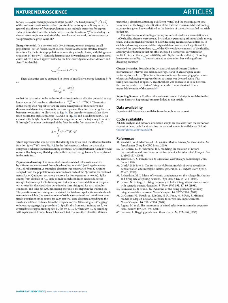
ArticlesNATuRe NeuROScIeNce
for α = 1, …, q in-focus populations at the point ∼r. The fixed points ∼∼ =α αrr r( *) *out of the in-focus equation (4) are fixed points of the entire system. It may occur, in general, that the out-of-focus populations attain multiple attractors for a given value of ∼r, in which case the set of effective transfer functions αF eff is labeled by the chosen attractor; in our analysis of the two-clustered network, only one attractor was present for a given value of ∼r.
Energy potential. In a network with Q = 2 clusters, one can integrate out all populations (out-of-focus) except one (in-focus) to obtain the effective transfer functions for the in-focus population representing a single cluster, with firing rate ∼r (equation (4) for q = 1). Network dynamics can be visualized on a one-dimensional curve, where it is well approximated by the first-order dynamics (see Mascaro and Amit31 for details):
∼∼ ∼τ = − +α
rt
r r rdd
( )syn,out
These dynamics can be expressed in terms of an effective energy function ∼E r( ) as
∼ ∼∼τ = −∂
∂αrt
E rr
dd
( )syn,
so that the dynamics can be understood as a motion in an effective potential energy landscape, as if driven by an effective force ∼ ∼∼
∼− = − −∂∂
r r r( ( ))E rr( ) out . The minima
of the energy with respect to ~r are the stable fixed points of the effective one-dimensional dynamics, whereas its maxima represent the effective energy barriers between two minima, as illustrated in Fig. 3c. The one-cluster network has three fixed points, two stable attractors (A and B in Fig. 3c) and a saddle point (C). We estimated the height, Δ, of the potential energy barrier on the trajectory from A to B through C as minus the integral of the force from the first attractor A to C:
∼ ∼ ∼∫Δ = −r r r r( ( ))dA
Cout
which represents the area between the identity line ∼=y r( )and the effective transfer function ∼=y r r( ( ))out (see Fig. 3c). In the finite network, where the dynamics comprise stochastic transitions among the states, switching between A and B would occur with a frequency that depends on the effective energy barrier Δ, as explained in the main text.
Population decoding. The amount of stimulus-related information carried by spike trains was assessed through a decoding analysis59 (see Supplementary Fig. 3 for illustration). A multiclass classifier was constructed from Q neurons sampled from the population (one neuron from each of the Q clusters for clustered networks, or Q random excitatory neurons for homogeneous networks). Spike counts from all trials of nstim taste stimuli in each condition (expected versus unexpected) were split into training and test sets for cross-validation. A template was created for the population peristimulus time histogram for each stimulus, condition, and time bin (200 ms, sliding over in 50-ms steps) in the training set. The peristimulus time histogram contained the trial-averaged spike counts of each neuron in each bin (the same number of trials across stimuli and conditions were used). Population spike counts for each test trial were classified according to the smallest euclidean distance from the templates across 10 training sets (‘bagging’ or bootstrap aggregating procedure60). Specifically, from each training set L, we created bootstrapped training sets Lb, for b = 1, …, B, where B = 10, by sampling with replacement from L. In each bin, each test trial was then classified B times
using the B classifiers, obtaining B different ‘votes’, and the most frequent vote was chosen as the bagged classification of the test trial. Cross-validated decoding accuracy in a given bin was defined as the fraction of correctly classified test trials in that bin.
The significance of decoding accuracy was established via a permutation test: 1,000 shuffled datasets were created by randomly permuting stimulus labels among trials, and a shuffled distribution of 1,000 decoding accuracies was obtained. In each bin, decoding accuracy of the original dataset was deemed significant if it exceeded the upper boundary, α0.05, of the 95% confidence interval of the shuffled accuracy distribution in that bin (this included a Bonferroni correction for multiple bins, so that α0.05 = 1 − 0.05/Nb, with Nb the number of bins). Decoding latency (insets in Fig. 1c,f) was estimated as the earliest bin with significant decoding accuracy.
Cluster dynamics. To analyze the dynamics of neural clusters (lifetime, interactivation interval, and latency, see Figs. 3 and 4), cluster spike count vectors ri (for i = 1, …, Q) in 5-ms bins were obtained by averaging spike counts of neurons belonging to a given cluster. A cluster was deemed active if its firing rate exceeded 10 spks s–1. This threshold was chosen so as to lie between the inactive and active clusters’ firing rates, which were obtained from a mean field solution of the network14.
Reporting Summary. Further information on research design is available in the Nature Research Reporting Summary linked to this article.
Data availabilityExperimental datasets are available from the authors on request.
Code availabilityAll data analysis and network simulation scripts are available from the authors on request. A demo code for simulating the network model is available on GitHub (https://github.com/mazzulab).
References 51. Zucchini, W. & MacDonald, I.L. Hidden Markov Models for Time Series: An
Introduction Using R (CRC Press, 2009). 52. La Camera, G. & Richmond, B. J. Modeling the violation of reward
maximization and invariance in reinforcement schedules. PLoS Comput. Biol. 4, e1000131 (2008).
53. Tuckwell, H. C Introduction to Theoretical Neurobiology (Cambridge Univ. Press, 1988).
54. Lánský, P. & Sato, S. The stochastic diffusion models of nerve membrane depolarization and interspike interval generation. J. Peripher. Nerv. Syst. 4, 27–42 (1999).
55. Richardson, M. J. Effects of synaptic conductance on the voltage distribution and firing rate of spiking neurons. Phys. Rev. E 69, 051918 (2004).
56. Brunel, N. & Sergi, S. Firing frequency of leaky intergrate-and-fire neurons with synaptic current dynamics. J. Theor. Biol. 195, 87–95 (1998).
57. Fourcaud, N. & Brunel, N. Dynamics of the firing probability of noisy integrate-and-fire neurons. Neural Comput. 14, 2057–2110 (2002).
58. La Camera, G., Rauch, A., Lüscher, H. R., Senn, W. & Fusi, S. Minimal models of adapted neuronal response to in vivo-like input currents. Neural Comput. 16, 2101–2124 (2004).
59. Rigotti, M. et al. The importance of mixed selectivity in complex cognitive tasks. Nature 497, 585–590 (2013).
60. Breiman, L. Bagging predictors. Mach. Learn. 24, 123–140 (1996).
NAtuRE NEuRosCiENCE | www.nature.com/natureneuroscience

1
nature research | reporting summ
aryO
ctober 2018
Corresponding author(s): Alfredo Fontanini
Last updated by author(s): Feb 13, 2019
Reporting SummaryNature Research wishes to improve the reproducibility of the work that we publish. This form provides structure for consistency and transparency in reporting. For further information on Nature Research policies, see Authors & Referees and the Editorial Policy Checklist.
StatisticsFor all statistical analyses, confirm that the following items are present in the figure legend, table legend, main text, or Methods section.
n/a Confirmed
The exact sample size (n) for each experimental group/condition, given as a discrete number and unit of measurement
A statement on whether measurements were taken from distinct samples or whether the same sample was measured repeatedly
The statistical test(s) used AND whether they are one- or two-sided Only common tests should be described solely by name; describe more complex techniques in the Methods section.
A description of all covariates tested
A description of any assumptions or corrections, such as tests of normality and adjustment for multiple comparisons
A full description of the statistical parameters including central tendency (e.g. means) or other basic estimates (e.g. regression coefficient) AND variation (e.g. standard deviation) or associated estimates of uncertainty (e.g. confidence intervals)
For null hypothesis testing, the test statistic (e.g. F, t, r) with confidence intervals, effect sizes, degrees of freedom and P value noted Give P values as exact values whenever suitable.
For Bayesian analysis, information on the choice of priors and Markov chain Monte Carlo settings
For hierarchical and complex designs, identification of the appropriate level for tests and full reporting of outcomes
Estimates of effect sizes (e.g. Cohen's d, Pearson's r), indicating how they were calculated
Our web collection on statistics for biologists contains articles on many of the points above.
Software and codePolicy information about availability of computer code
Data collection Single units were isolated using a template algorithm, clustering techniques, and examination of inter-spike interval plots (Offline Sorter, Plexon).
Data analysis All data analyses, model simulations and mean field theory All calculations were performed using custom software written in MATLAB R2017b (MathWorks), and C.
For manuscripts utilizing custom algorithms or software that are central to the research but not yet described in published literature, software must be made available to editors/reviewers. We strongly encourage code deposition in a community repository (e.g. GitHub). See the Nature Research guidelines for submitting code & software for further information.
DataPolicy information about availability of data
All manuscripts must include a data availability statement. This statement should provide the following information, where applicable: - Accession codes, unique identifiers, or web links for publicly available datasets - A list of figures that have associated raw data - A description of any restrictions on data availability
A demo code for simulating the network model in the expected and unexpected conditions will be available at publication on GitHub (https://github.com/mazzulab).
Field-specific reportingPlease select the one below that is the best fit for your research. If you are not sure, read the appropriate sections before making your selection.
Life sciences Behavioural & social sciences Ecological, evolutionary & environmental sciences

2
nature research | reporting summ
aryO
ctober 2018For a reference copy of the document with all sections, see nature.com/documents/nr-reporting-summary-flat.pdf
Life sciences study designAll studies must disclose on these points even when the disclosure is negative.
Sample size No statistical methods were used to pre-determine sample sizes but our sample sizes are similar to those reported in previous publications.
Data exclusions Only experimental sessions yielding ensembles of five or more simultaneously recorded neurons were included in the analyses, due to the statistical constraints inherent in the hidden Markov model analysis.
Replication We have run our simulations multiple times and we are able to reproduce our conclusions.
Randomization Each network was initialized with random synaptic weights and simulated with random initial conditions. Stimulus and cue selectivities were assigned to randomly chosen sets of neurons in each network.
Blinding Not relevant - there were no experimental groups.
Reporting for specific materials, systems and methodsWe require information from authors about some types of materials, experimental systems and methods used in many studies. Here, indicate whether each material, system or method listed is relevant to your study. If you are not sure if a list item applies to your research, read the appropriate section before selecting a response.
Materials & experimental systemsn/a Involved in the study
Antibodies
Eukaryotic cell lines
Palaeontology
Animals and other organisms
Human research participants
Clinical data
Methodsn/a Involved in the study
ChIP-seq
Flow cytometry
MRI-based neuroimaging
Copyright © 2022 FDOKUMEN