arX

iv:a

dap-

org/

9907

002v

1 2

Jul

199

9

Metastable Evolutionary Dynamics:

Crossing Fitness Barriers or

Escaping via Neutral Paths?

Erik van Nimwegen∗ and James P. Crutchfield

Santa Fe Institute, 1399 Hyde Park Road, Santa Fe, NM 87501Electronic addresses: erik,chaos@santafe.edu

(February 14, 2013)

We analytically study the dynamics of evolving populations that exhibit metastabilityon the level of phenotype or fitness. In constant selective environments, such metastablebehavior is caused by two qualitatively different mechanisms. One the one hand, populationsmay become pinned at a local fitness optimum, being separated from higher-fitness genotypesby a fitness barrier of low-fitness genotypes. On the other hand, the population may only bemetastable on the level of phenotype or fitness while, at the same time, diffusing over neutralnetworks of selectively neutral genotypes. Metastability occurs in this case because thepopulation is separated from higher-fitness genotypes by an entropy barrier: The populationmust explore large portions of these neutral networks before it discovers a rare connectionto fitter phenotypes.

We derive analytical expressions for the barrier crossing times in both the fitness barrierand entropy barrier regime. In contrast with “landscape” evolutionary models, we show thatthe waiting times to reach higher fitness depend strongly on the width of a fitness barrier andmuch less on its height. The analysis further shows that crossing entropy barriers is fasterby orders of magnitude than fitness barrier crossing. Thus, when populations are trapped ina metastable phenotypic state, they are most likely to escape by crossing an entropy barrier,along a neutral path in genotype space. If no such escape route along a neutral path exists,a population is most likely to cross a fitness barrier where the barrier is narrowest, ratherthan where the barrier is shallowest.

Santa Fe Institute Working Paper 99-07-041Keywords: Populations dynamics, neutral networks,

fitness barrier, entropy barrier, metastability.Running Head: Metastable Evolutionary Dynamics

Contents

I Introduction 2

A Evolutionary Pathways andMetastability . . . . . . . . . . . . . 3

B Overview . . . . . . . . . . . . . . . 4

II Evolutionary Dynamics 4

III Crossing a Single Barrier 5

A Metastable Quasispecies . . . . . . 6

B Valley Lineages . . . . . . . . . . . 7

C Crossing the Fitness Barrier . . . . 9

D Additional Time in Valley Bushes . 10

E Theory versus Simulation . . . . . . 10

F Scaling of the Barrier Crossing Time 12

∗Permanent address: Bioinformatics Group, University of Utrecht, Padualaan 8, NL-3584-CH Utrecht, TheNetherlands

1

IV The Entropy Barrier Regime 15

A Error Thresholds . . . . . . . . . . 15

B The “Landscape” Regime . . . . . . 16

C Time Scales in the Entropic Regime 17

D Anomalous Scaling . . . . . . . . . 18

V Traversing Complex Fitness Func-

tions 20

A The Royal Staircase with Ditches . 20

B Evolutionary Dynamics . . . . . . . 21

C Observed Population Dynamics . . 22

D Epoch Quasispecies and The Sta-tistical Dynamics Approach . . . . 23

E Crossing the Fitness Barrier . . . . 24

F Theoretical and ExperimentalEpoch Times . . . . . . . . . . . . . 25

VI Conclusions 28

APPENDIXES 31

A Analytical Approximation of the

Epoch Quasispecies 31

I. INTRODUCTION

For populations evolving under selection, muta-tion, and a static fitness function, there are twomain mechanisms thought to be responsible for theoccurrence of dynamical metastability—a behaviorcommonly observed in natural and artificial evolu-tionary processes [1–3,8,10,23] and called punctuated

equilibria in paleobiology [13]. First, a populationmay become trapped around a local optimum in thefitness “landscape” until a rare mutant crosses a fit-

ness barrier to a higher nearby peak. Second, morerecently it has been proposed [10,15,29] that popu-lations may evolve neutrally, drifting randomly overneutral networks of isofitness genotypes in genotypespace, until a rare single-point mutant connection isfound to another neutral network of higher fitness.In this case, the population must cross an entropy

barrier by visiting a large volume of the neutral net-work before it discovers a path to higher fitness.

To understand the relative roles of these twomechanisms in evolutionary metastability, in the fol-lowing we study the dynamics of a population evolv-ing under simple fitness functions that contain asingle fitness barrier of tunable height and width.In order for the population to escape its currentmetastable state and so reach higher fitness, it mustcreate a genotype that is separated from the cur-rent fittest genotypes in the population by a valley

of lower-fitness genotypes. The height of the fitnessbarrier measures the relative selective difference be-tween the current fittest genotypes and the lower-fitness genotypes in the intervening valley. Its width

denotes the number of point mutations the currentfittest genotypes must undergo to cross the valley oflow fitness genotypes. We derive explicit analyticalpredictions for the barrier crossing times as a func-tion of population size, mutation rate, and barrierheight and width. The scaling of the fitness-barriercrossing time as a function of these parameters showsthat the waiting time to reach higher fitness dependscrucially on the width of the barrier and much lesson the barrier height.

This contrasts with the scaling of the barrier cross-ing time for a particle diffusing in a double-wellpotential—a model proposed previously for popu-lations crossing a fitness barrier [20,22]. For suchstochastic processes, it is well known that the wait-ing time scales exponentially with the barrier height[12]. In the population dynamics that we analyzehere, we find that the waiting time scales approxi-mately exponential with barrier width and only asa power law of the logarithm of barrier height. Inaddition, the waiting time scales roughly as a powerlaw in both population size and mutation rate.

When the barrier height is lowered below a criticalheight, the fitness barrier turns into an entropy bar-rier. We show that, in general, neutral evolution viacrossing entropy barriers is faster by orders of mag-nitude than fitness barrier crossing. Additionally,we show that the waiting time for crossing entropybarriers exhibits anomalous scaling with populationsize and mutation rate.

Finally, we extend our analysis to a class of morecomplicated fitness functions that contain a networkof tunable fitness and entropy barriers. We showthat the theory still accurately predicts fitness- andentropy-barrier crossing times in these more compli-cated cases.

The general conclusion drawn from our analysis isthat, when populations are trapped in a metastable

2

phenotypic state, they are most likely to escape thismetastability by crossing an entropy barrier. Thatis, the escape to a new phenotype occurs along aneutral path in genotype space. If no such neutralpath exists, then the population is most likely tocross a fitness barrier at the place where the barrieris narrowest.

A. Evolutionary Pathways and Metastability

The notion of an adaptive landscape, first intro-duced by Wright [32], has had a large impact onour appreciation of the mechanisms that control howpopulations evolve in static environments. The in-tuitive idea is that a population moves up the slopesof its fitness “landscape” just as a physical systemmoves down the slope of its potential-energy surface.Once this analogy has been accepted, it is naturalto borrow many of the qualitative results on the dy-namics of physical systems to account for the dy-namics of evolving populations. For instance, it hasbecome common to assume that an evolving popu-lation can be modeled by a single uphill walker in a“rugged” fitness landscape [16,21].

There are, however, seemingly different kinds ofevolutionary behavior than incremental adaptationvia “landscape” crawling. For example, metastabil-ity or punctuated equilibrium of phenotypic traitsin an evolving population appears to be a commonoccurrence in biological evolution [8,13] as well as inmodels of natural and artificial evolution [1,3,10]. Asjust pointed out, for simple cases where populationsevolve in a relatively constant environment, thereare two main mechanisms that have been proposedto account for this type of metastable behavior.

The first and most commonly accepted explana-tion was already implicit in Wright’s shifting balance

theory [33]. A population moves up the slope of itsfitness “landscape” until it reaches a local optimum,where it stabilizes. The population is pictured asa cloud in genotype space focused around this lo-cal optimum. The population remains in this stateuntil a rare sequence of mutants crosses a valley oflow fitness towards a higher fitness peak. In thisview, metastability is the result of fitness barriers

that separate local optima in genotype space.

This mechanism for metastability is very reminis-cent of that found in physical systems. Metastabilityoccurs there because local energy minima in state

space are separated by potential energy barriers,which impede the immediate transition between theminima. A physical system generally moves throughits state space along trajectories that lower its en-ergy. Once it reaches a local minimum it tends tostay there. However, when such a system is sub-ject to thermal fluctuations, through a sequence ofchance events it can eventually be pushed over a bar-rier that separates the current local minimum fromanother. When this transition occurs, it turns outthat the system moves quickly to the new local min-imum.

Mathematically, barrier crossing processes inphysical systems are most often described as diffu-sion in a potential field, where the potential repre-sents the energy “landscape”. These processes havebeen extensively studied and the basic quantitativeresults are widely known [11,12,26]. For example,barrier crossing times increase exponentially withthe height of the barrier and inverse exponentiallywith the fluctuation amplitude, as measured by tem-perature.

In light of the physical metaphor for evolving pop-ulations, it is not surprising that the dynamics ofpopulations crossing fitness barriers has been mod-eled using a class of diffusion equations analogousto those used to describe thermally driven systemsin a potential [20,22]. In this approach, the dy-namics of the average fitness of the population ismodeled as diffusion over the “fitness landscape”,thermal fluctuations are replaced by random geneticmutations and drift, and the population size, whichcontrols sampling stochasticity, plays the role of in-verse temperature. As a direct consequence, it wasfound that fitness-barrier crossing times scale expo-nentially with population size in these models. Notethat it is assumed in this approach that the popula-tion as a whole must cross the fitness barrier.

In the following, we show that the analogy withthe physical situation and, in particular, the trans-lation of results from there are misleading for theunderstanding of the evolutionary dynamics. Forexample, a direct analysis of the population dynam-ics reveals that for most parameter ranges, the timeto cross a fitness barrier scales very differently forpopulations evolving under selection and mutation.For example, the waiting time is determined by howlong it takes to generate a rare sequence of mutants

that crosses the fitness barrier, as opposed to howlong it takes the population as a whole to cross thefitness barrier.

3

This brings us to the second main mechanism formetastability—one that has been put forward morerecently [2,10,15,23,29]. The second mechanism de-rives from the observation that large sets of mu-tually fitness-neutral genotypes are interconnectedalong single-point mutation paths. That is, sets ofisofitness genotypes form extended neutral networks

under single-point mutations in genotype space.

In this alternative scenario, a population displaysa constant distribution of phenotypes for some pe-riod while, at the same time, individuals in thepopulation diffuse over a neutral network in geno-type space. That is, despite phenotypic metastabil-ity, there is no genotypic stasis during this period.The phenotype distribution remains metastable un-til, via diffusion over the neutral network, a memberof the population discovers a genotypic connectionto a higher-fitness neutral network.

When this mechanism operates, metastability isthe result of an entropy barrier, as we call it. Thepopulation must spread over or search large parts ofthe neutral network before it finds a connection toa higher-fitness network. One envisages the popula-tion moving randomly through a genotypic labyrinthof common phenotypes with only a single or rela-tively few exits to fitter phenotypes.

B. Overview

In the following, we analyze and compare the pop-ulation dynamics of crossing such fitness and entropybarriers with the goals of elucidating the basic mech-anisms responsible for each, calculating the scalingforms for the evolutionary times scales associatedwith each, and understanding their relative impor-tance when both can operate simultaneously.

Section II defines the basic evolutionary model.

Section III introduces a tunable fitness functionthat models the simplest case in which to studyboth types of barrier crossing. It consists of a sin-gle local optimum, with a valley, and a single por-tal (target genotype) in genotype space. By tuningthe height of the local optimum one can change thefitness barrier into an entropy barrier. We analyzethis basic model as a branching process, calculat-ing the statistics of lineages of individuals in thefitness valley. Comparison of the theoretical pre-dictions for the fitness-barrier crossing times withdata obtained from simulations shows that the the-

ory accurately predicts these fitness-barrier crossingtimes for a wide range of parameters. We also de-rive several simple scaling relations for the fitness-barrier crossing times appropriate to different pa-rameter regimes.

Section IV first determines the barrier heights atwhich the fitness-barrier regime shifts over into anentropic one. After this, we discuss the popula-tion dynamics of crossing entropy barriers, provid-ing rough scaling relations for the barrier crossingtimes in this regime. Comparison of these resultswith the scaling relations for fitness-barrier cross-ing shows that entropy-barrier crossing proceedsmarkedly faster than crossing fitness barriers.

Section V extends our analysis to a set of muchmore complicated fitness functions—a class calledthe Royal Staircase with Ditches. These fitness func-tions are closely related to the Royal Road [29,30]and Royal Staircase [27,28] fitness functions that westudied earlier, which consist of a sequence or a net-work of entropy barriers only. The Royal Staircasewith Ditches generalizes this class of fitness func-tions to one that possesses multiple fitness and en-tropy barriers of variable width, height, and volume.We adapt the theoretical analysis using our statisti-cal dynamics approach [30] to deal with these morecomplicated, but more realistic cases. Comparisonof the theoretically predicted and experimentally ob-tained barrier crossing times again shows that thetheory accurately predicts the barrier crossing timesin these more complicated situations as well.

Finally, Sec. VI presents our conclusions and dis-cusses the general picture of metastable populationdynamics that emerges from our analyses.

II. EVOLUTIONARY DYNAMICS

We consider a simple evolutionary dynamics ofselection and mutation with a constant populationsize M . An individual’s genotype consists of a bi-nary sequence of on-or-off genes. We consider thesimple case in which the fitness of an individual isdetermined by its genotype only. The genotype-to-phenotype and phenotype-to-fitness maps are col-lapsed into a direct determination of a genotype’sfitness. Selection and reproduction are assumed totake place in discrete generations, with mutation oc-curring at reproduction. The exact evolutionary dy-namics is defined as follows.

4

• A population consists of M binary sequencesof a fixed size L.

• A fitness fs is associated with each of the 2L

possible genotypes s ∈ AL, where A = 0, 1.

• Every generation M individuals in the currentpopulation are sampled with replacement andwith a probability proportional to their fitness.Thus, the expected number of offspring for anindividual with genotype s is fs/〈f〉, where 〈f〉is the current average fitness of the population.

• Once the M individuals have been selected,each bit in each individual is mutated (flipped)with probability µ, the mutation rate.

In this basic model there are effectively two evolu-tionary parameters: the mutation rate µ and thepopulation size M .

Several aspects of the basic model—such as, dis-crete generations and fixed population size—weremainly chosen for analytical convenience. Thediscrete-generation assumption can be lifted, lead-ing to a continuous-time model, without affectingthe results presented below. As for the assumptionof fixed population size, the analysis can be adaptedin a straightforward manner to address (say) fluctu-ating or exponentially growing populations.

Models including genetic recombination are no-toriously more difficult to analyze mathematically.Despite our interest in the effects of recombina-tion, it is not included here largely for this reason.Moreover, for wide parameter ranges in the neutraland piecewise-neutral evolutionary processes we con-sider, it appears that recombination need not be adominant mechanism. For example, Refs. [30, sec.6.5] and [28, sec. VIII] show that recombination of-ten does not significantly affect population dynamicsin these cases.

III. CROSSING A SINGLE BARRIER

We first consider the simple case of a single bar-rier for the population to cross. Of the 2L geno-types, there is one with fitness σ > 1 that we referto as the peak genotype Π. Then there are 2L − 2genotypes with fitness 1 that we refer to as valley

genotypes. Finally, there is a single portal genotypeΩ at a Hamming distance w from the fitness-σ peakgenotype Π. We view the portal genotype as giving

access to higher-fitness genotypes—genotypes whosedetails are unimportant, since in this section we onlyanalyze the dynamics up to the portal’s first discov-ery.

The variable w tunes the fitness barrier’s width

and the variable σ its height. The height σ also in-dicates a peak individual’s selective advantage overthose in the valley, as measured by the relative dif-ference σ − 1 of their expected number of offspring.Figure 1 illustrates the basic setup.

Peakf = σ

Valleyf = 1

↑ Fitness

ΩPortal

Π

w

A L

FIG. 1. Evolution from the peak genotype Π to thehigher-fitness portal genotype Ω via low-fitness valleygenotypes. The selective advantage of the peak indi-viduals over those in the valley is controlled by the peakheight σ. The portal and peak genotypes are a Ham-ming (mutational) distance w apart. The domain is thehypercube AL of all length-L genotypes.

At time t = 0 the population starts with all Mgenotypes located at the peak Π. We then evolvethe population under selection and mutation, as de-scribed in the previous section, until the portal geno-type Ω occurs in the population for the first time.(Hence, the portal’s fitness is not relevant.) This de-fines one evolutionary run. We record the time t atwhich the portal is discovered. We are interested inthe average discovery time 〈t〉, averaged over an en-semble of such runs. We are particularly interestedin the scaling of this barrier crossing time 〈t〉 as afunction of the evolutionary parameters M and µ,as well as the barrier parameters σ and w.

Let’s briefly review in simple language the evolu-tionary dynamics before launching into the math-ematical analysis. In the parameter regime withσ ≫ 1, where the peak fitness is considerably largerthan the valley fitness, and with the mutation rate µnot too high, the bulk of the population remains atthe peak. That is, the population is a quasispecies

cloud, centered around the peak genotype Π [7]. For

5

such parameter regimes, the barrier is clearly a fit-ness barrier: the waiting time 〈t〉 is determined bythe time it takes to create a rare sequence of mutantgenotypes that crosses the valley between the peakand the portal.

However, as σ → 1+, the fitness barrier trans-forms into an entropy barrier. For σ = 1 there is nofitness difference between peak and valley genotypesand the entire population simply diffuses throughgenotype space until the portal is discovered. As wewill see below, the entropic regime sets in rather sud-denly at a value of σc somewhat above σ = 1. As weshow, this transition is the well known error thresh-

old of molecular evolution theory [6]. At σ = σc,the value of which depends on the population sizeM and mutation rate µ, the subpopulation on thepeak becomes unstable in the sense that all individ-uals on the peak may be lost through a fluctuation.More precisely, the waiting time for such a fluctu-ation to occur becomes short in comparison to thefitness-barrier crossing time. When this fluctuationhas occurred, there is no longer a restoring “force”that keeps the population concentrated around thepeak genotype. The population as a whole diffusesrandomly through the valley as if the genotypes wereall fitness neutral. While our analysis accurately pre-dicts the barrier crossing times in the fitness-barrierregime, it is notable that beyond the error threshold,in the entropic regime, only order-of-magnitude pre-dictions can be obtained using the current analyticaltools.

Calculating the barrier crossing time proceeds inthree stages. First, in Sec. III A we determine thepopulation’s quasispecies distribution, defined as theaverage proportions of individuals located on thepeak and in the valley during the metastable state.From this, one directly calculates the average fitnessin the population. Second, in Sec. III B we considerthe genealogy statistics of individuals in the valley.In the fitness-barrier regime, genealogies in the val-ley are generally short-lived and are all seeded bymutants of the peak genotype. We approximate theevolution of valley genealogies as a branching processand use this representation to calculate the averagebarrier crossing time. Third, with this analysis com-plete, Sec. VE then addresses the transition fromthe fitness-barrier regime to the entropic one.

A. Metastable Quasispecies

Each evolutionary run, the population starts outconcentrated at the peak genotype Π. After a relax-ation phase, assumed to be short compared to thebarrier crossing time, there will be roughly constantproportions of the population on the peak and in thevalley. We now calculate the equilibrium proportionPΠ of peak individuals and the population’s averagefitness 〈f〉, after this relaxation phase.

To first approximation, one can neglect back mu-

tations from valley individuals back into the peakgenotype. First of all, if σ ≫ 1, selection keeps thebulk of the population on the peak. Additionally,valley individuals produce fewer offspring than peakindividuals and they are unlikely—with a probabil-ity 1/L at most—to move back onto the peak whenthey mutate. In this regime, the quasispecies dis-tribution is largely the result of a balance betweenselection expanding the peak population by a factorof σ/〈f〉 and deleterious mutations moving them intothe valley with probability 1−(1−µ)L. The result isthat we have a balance equation for the proportionPΠ of peak individuals given by

PΠ =σ

〈f〉(1 − µ)LPΠ . (1)

From this we immediately have that

〈f〉 = σ(1 − µ)L . (2)

Since we also have that 〈f〉 = σPΠ +1 · (1−PΠ), wecan determine the proportion of peak individuals tobe:

PΠ =〈f〉 − 1

σ − 1. (3)

For parameters where 〈f〉 = σ(1 − µ)L ≫ 1, Eqs.(2) and (3) give quite accurate predictions for theaverage fitness and the proportion of individuals onthe peak.

In cases where 〈f〉 is close to 1, a substantial pro-portion of the population is located in the valleyand back mutations from the valley onto the peakmust be taken into account. To do this, we intro-duce the quasispecies Hamming distance distribu-

tion ~P = (P0, . . . , Pi, . . . , PL), where Pi is the pro-portion of individuals located at Hamming distancei from Π. Thus, P0 = PΠ indicates the proportion

6

on the peak. Under selection, the distribution ~Pchanges according to:

P seli =

(σ − 1)δi0 + 1

〈f〉Pi , (4)

where δij = 1, if i = j, and δij = 0, otherwise. Wecan write this formally as the result of an operator

acting on ~P :

~P sel =

(

S · ~P)

i

〈f〉, (5)

where

Sij = [(σ − 1)δi0 + 1] δij , (6)

defines the selection operator S.

Next, we consider the transition probabilities Mij

that under mutation a genotype at Hamming dis-tance j from the peak moves to a genotype at Ham-ming distance i from the peak. We have that:

Mij =

L−j∑

u=0

j∑

d=0

δj+u−d,i

(L − j

u

)(j

d

)

×µu+d(1 − µ)L−u−d . (7)

That is, Mij is the sum of the probabilities of allpossible ways to mutate u of the L − j bits sharedwith Π and d of the j bits that differ, such thatj + u − d = i. Equation (7) defines the mutation

operator M.

We can now introduce the generation operator

G = M · S. The equilibrium quasispecies distri-

bution ~P is a solution of the equation

~P =G · ~P

〈f〉. (8)

In this way, the quasispecies distribution is givenby the principal eigenvector, normalized in proba-bility, of the matrix G; while the average fitness 〈f〉is given by G’s principal eigenvalue. Note that this isconventional quasispecies theory [7], apart from thefacts that we have grouped the quasispecies mem-bers into Hamming-distance classes and that we con-sider discrete generations, rather than continuoustime.

B. Valley Lineages

Under the approximation that back mutationsfrom the valley onto the peak can be neglected, aroughly constant proportion 1 − PΠ of valley indi-viduals is maintained by a roughly constant influxof mutants from the peak. Every generation, somepeak individuals leave mutant offspring in the val-ley. Additionally, each valley individual leaves onaverage a fraction 1/〈f〉 offspring in the next gener-ation, as can be seen from Eq. (4). This means thatthe fraction of valley individuals, for which all of itst ancestors in the previous t generations were val-ley individuals as well, is only 1/〈f〉

t. For 〈f〉 ≫ 1,

this implies in turn that whenever a peak individualseeds a new lineage of valley individuals by leavinga mutant offspring in the valley, this lineage is un-likely to persist for a large number of generations. Inother words, lineages composed of valley individualsare short lived.

Intuitively, the idea is that the preferred selectionof peak individuals leads to a “surplus” of peak off-spring that spills into the valley through mutations.Each mutant offspring of a peak individual forms theroot of a relatively small, i.e., short-lived, genealog-ical tree of valley individuals. The barrier crossingtime is determined essentially by the waiting timeuntil one of these genealogical bushes produces a de-scendant that discovers the portal. These processesare illustrated in Fig. 2.

Peakf = σ

Valleyf = 1

Time →

↑ Fitness

ΩPortal

Π

FIG. 2. Genealogies during fitness-barrier crossing.An example genealogical tree is sketched for peak in-dividuals (above); they have fitness σ and are copies ofthe peak genotype Π. The valley individuals (below) atlower fitness occur in genealogies that are seeded (dashedlines) from peak individuals. These genealogies are rel-atively short-lived bushes. Evolution continues until thetime at which one of the valley bushes discovers the por-tal genotype Ω.

7

We will analyze the evolution of a valley lineageas a branching process [14]. The probability On thatone particular valley individual leaves n offspring inthe next generation is given by a binomial distribu-tion. This is well approximated by a Poisson distri-bution as follows:

On =

(M

n

)(1

M〈f〉

)n(

1 −1

M〈f〉

)M−n

≈1

n!

(1

〈f〉

)n

e−1/〈f〉 . (9)

To a good approximation, we may treat the evo-lution of each valley lineage as independent of theother valley lineages. Under this approximation,each valley individual independently has a distribu-tion of offspring given by Eq. (9). Of course, underfixed population size, the independence assumptionmay break down when valley lineages dominate thepopulation.

We now calculate the probability that a valley lin-eage produces a descendant that discovers the portalΩ before the lineage goes extinct. Let a valley lin-eage be founded by an ancestor in the valley that islocated at Hamming distance j from Ω. We denoteby pj(t) the probability that t generations from now,none of this ancestor’s descendants will have discov-ered the portal. This probability can be determinedrecursively, in terms of the probabilities pi(t − 1) asfollows,

pj(t) = O0 + O1

L∑

i=1

pi(t − 1)Mij (10)

+ O2

L∑

i,k=1

pi(t − 1)Mij pk(t − 1)Mkj + . . . .

The first term in the above equation correspondsto the ancestor having no offspring. This, of course,ensures that the portal will not be discovered t gen-erations from now, since leaving zero offspring im-plies that the genealogy goes extinct immediately.The second term corresponds to the ancestor havingone offspring, at Hamming distance i from the por-tal, that will not give rise to discovery of the portal.That is, since this offspring itself forms the ancestorof a new valley lineage, pi(t − 1) gives the probabil-ity that none of its descendants discovers the portalwithin the next t−1 generations. The third term cor-responds to the ancestor having two offspring, oneat distance i from the portal and one at distance k,

neither of which give rise to the discovery of Ω. Thehigher-order terms in Eq. (10) correspond to theancestor having 3, 4, and more offspring.

Recall that the mutation operator Mij , as definedin Eq. (7), gave the probability to go from Ham-ming distance j to distance i from the peak undermutation. Mij appears above in Eq. (10) with adifferent, but equivalent, meaning: Mij there givesthe probability to go from a Hamming distance j toa distance i from the portal under mutation. Thisuse of Mij appears repeatedly in the following.

Using Eq. (9) we can sum the series in Eq. (10),obtaining:

pj(t) = e([p(t−1)·M]j−1)/〈f〉 , (11)

where p(t) = (p1(t), p2(t), . . . , pL(t)) and the vectornotation denotes the sum

[p(t − 1) · M]j =L∑

i=1

pi(t − 1)Mij . (12)

For 〈f〉 ≥ 1, a valley genealogy eventually eitherdiscovers Ω or goes extinct; see, for instance, Ref.[14]. Letting t → ∞ in Eq. (11), we obtain a set ofnonlinear equations for the asymptotic probabilitiespj that a genealogical bush, whose founder startedat Hamming distance j from Ω, goes extinct beforeany of its descendants discovers the portal. Theseare given by

pj = e([p·M]j−1)/〈f〉 . (13)

Equations (13) appear to be unsolvable in closedanalytical form. Their solutions may be numericallyapproximated in a straightforward manner; for in-stance, by simply iterating Eq. (11). However, inthe regime where µ is small and 〈f〉 is not too closeto 1, the probabilities pi are generally very close to1. In this regime, one may expand Eq. (13) to firstorder around pi = 1. To do this, we introduce theprobabilities ǫi = 1− pi that the portal does get dis-covered by the lineage before it goes extinct. To firstorder in ǫi we obtain from Eq. (13) the equationsgiven by

ǫj = 1 − e−M0j/〈f〉

(

1 −[ǫ ·M]j〈f〉

)

, (14)

where ǫ = (ǫ1, . . . , ǫL). These equations can be eas-ily inverted, yielding:

8

ǫj =

L∑

i=1

(

1 − e−M0i/〈f〉)

(I− R)−1ij , (15)

where I is the identity matrix and the matrix R hascomponents

Rij =Mij

〈f〉e−M0j/〈f〉 . (16)

Note that the indices i and j in the matrices run from1 to L, corresponding to ancestors at Hamming dis-tances between 1 and L from the portal. Note alsothat, by definition, ǫ0 = 1.

To first order, Eqs. (15) give the probabilities ǫj

that a valley lineage, founded by an ancestor at aHamming distance j from Ω, discovers the portalbefore the lineage goes extinct. Now to calculatethe barrier crossing time we just have to determinethe number of new valley lineages that are foundedper generation.

C. Crossing the Fitness Barrier

Every generation, M individuals are selected inproportion to their fitness. Each such selection maylead to the seeding of a new lineage in the valley.The probability P not that a selection will not leadto the founding of a new valley lineage is given by:

P not =1 − PΠ

〈f〉+

σ

〈f〉PΠ(1 − µ)L . (17)

The first term corresponds to selecting a valley in-dividual, that by definition is already on a lineage.The second term corresponds to a peak individualbeing selected and reproducing without mutation,leaving an offspring on the peak.

The probability P seedj that a new lineage will be

seeded in the valley and at a Hamming distance jfrom Ω is given by

P seedj =

σ

〈f〉PΠ

[Mjw − (1 − µ)Lδjw

], (18)

where w is the Hamming distance between the peakand the portal. The first factor, σPΠ/〈f〉, gives theprobability that a peak individual will be selected.The term Mjw is the probability that under muta-tion this peak individual moves from Hamming dis-tance w to distance j from the portal. For j 6= w

this always corresponds to a new lineage in the val-ley. For j = w, we must discount for the probabilitythat the peak individual did not undergo any muta-tions at all. This is given by the term (1 − µ)Lδjw .

Putting these together, we find the probabilityP sel, that a selection does not seed a lineage leadingto the portal, is given by

P sel = P not +

L∑

j=1

(1 − ǫj)Pseedj . (19)

Using Eqs. (13), (17), and (18) and the identity〈f〉 = 1 + (σ − 1)PΠ, Eq. (19) can be rewritten as

P sel = 1 +σ(〈f〉 − 1)

(σ − 1)〈f〉

×[(1 − µ)Lǫw + 〈f〉 log(1 − ǫw)

]. (20)

Expanding the logarithm to first order in ǫw, and us-ing the approximation in Eq. (2) for 〈f〉, we obtainthe simple expression

P sel = 1 − ǫw(〈f〉 − 1). (21)

The probability that none of the M selectionsfrom the current generation seeds a lineage that dis-

covers the portal is simply(P sel

)M. By our as-

sumption of a roughly constant quasispecies distri-bution, this probability is constant. Thus, the ex-pected number 〈t〉 of generations until a lineage willbe seeded that discovers the portal is given by

〈t〉 =1

1 −(P sel

)M≈

1

M(〈f〉 − 1)ǫw. (22)

where ǫw is given by Eqs. (15) and (16).

Equation (22) constitutes our theoretical predic-tion for the average barrier crossing time 〈t〉 as afunction of the population size M , the fitness differ-ential σ between the peak and the valley, the muta-tion rate µ, the string length L, and the width w ofthe fitness barrier. To obtain it, we made several ap-proximations. We assumed that σ was large enoughand µ small enough such that 〈f〉 was substantiallylarger than 1. Under those assumptions, lineages inthe valley are short lived, the total number of indi-viduals in the valley will be small with respect to M ,and the probabilities ǫi will be small. This justifiesour leading-order expansion for 〈t〉.

9

D. Additional Time in Valley Bushes

Equation (22) gives the average number 〈t〉 of gen-erations until a lineage is founded that discovers theportal. The actual average time until the portal isdiscovered is somewhat longer, since the lineage thatfinds the portal itself takes a certain average numberof generations to discover the portal. Specifically,there is an additional average time, that we denoteby 〈dt〉, between the founding of the first lineage thatdiscovers the portal and the actual discovery of Ω.

We can directly approximate this correction term〈dt〉 when the ǫi are small. As we will see below,generally 〈dt〉 ≪ 〈t〉 in the parameter regime whereour approximations are valid. This makes the effectof including the correction term 〈dt〉 rather small inthese parameter regimes. However, as we approachthe parameter regime where the ǫi become large, theaverage number of generations 〈t〉 until the found-ing of the lineage that discovers the portal becomescomparable to the average number of generations〈dt〉 that it takes this lineage to actually discoverthe portal. In this (limited) parameter regime, in-cluding the correction term 〈dt〉 leads to a significantimprovement of our theoretical predictions.

Paralleling the development of the Eq. (13), westart by expanding Eq. (11) to first order in ǫj(t);the probability that the lineage starting at distancej has discovered the portal by time t. We find that

ǫj(t) = 1 − e−M0j/〈f〉

(

1 −[ǫ(t − 1) ·M]j

〈f〉

)

. (23)

The expected additional time 〈dtj〉, given that thelineage started at a Hamming distance j from Ω andconditioned on the lineage discovering the portal, isformally given by

〈dtj〉 =

∞∑

t=1

tǫj(t) − ǫj(t − 1)

ǫj

=

∞∑

t=0

ǫj − ǫj(t)

ǫj, (24)

where the asymptotic ǫj is given by Eqs. (15) and(16). Using Eq. (23) and the boundary conditionsǫj(0) = 0, the above sum gives:

〈dtj〉 =1

ǫj

L∑

i=1

(

1 − e−M0i/〈f〉)

(I− R)−2ij , (25)

where the matrix R is again defined by Eq. (16).

In order to obtain 〈dt〉 we have to weigh each ofthe times 〈dtj〉 with a factor cj corresponding to therelative proportion of times that a lineage startingat Hamming distance j discovers the portal. Thatis, averaged over an ensemble of runs, cj is the pro-portion of times that the portal was discovered bya lineage that started at Hamming distance j. Theweight cj should be proportional to both the proba-bility ǫj and the rate of creating of lineages at Ham-ming distance j from the portal. We have that

cj =ǫj

(Mjw − (1 − µ)Lδjw

)

∑

k ǫk (Mkw − (1 − µ)Lδkw),

j = 0, 1, . . . , L , (26)

where the factors in parentheses are similar to thatfound in Eq. (18). It should be noted that herethe indices run from 0 to L and not from 1 to L,since the portal may also be discovered by a jumpmutation directly from the peak.

Combining Eqs. (25) and (26) and using Eq. (15),we find that the average length of the valley bushthat discovers the portal is

〈dt〉 =

[ǫ · (I − R) ·

(M − I(1 − µ)L

)]

w

[ǫ · (M − I(1 − µ)L)]w + M0w, (27)

where, again, ǫ is given by its components in Eqs.(15) and (16). The indices in the vector notationnow run from 1 to L.

Adding the correction term 〈dt〉 to 〈t〉 as givenby Eq. (22) improves our theoretical predictions es-pecially in the regime where the ǫi become large.However, we still expect the approximations leadingto the above equations for 〈t〉 and 〈dt〉 to break downwhen 〈f〉 → 1+.

E. Theory versus Simulation

We simulated an evolving population using a fit-ness function consisting of a single barrier, as de-scribed in Secs. II and III, for a wide range of param-eter settings to quantitatively test our theoreticalpredictions. Results for several parameter regimesare shown in Fig. 3, where the simulation resultsare plotted using dashed lines and the theoretical

10

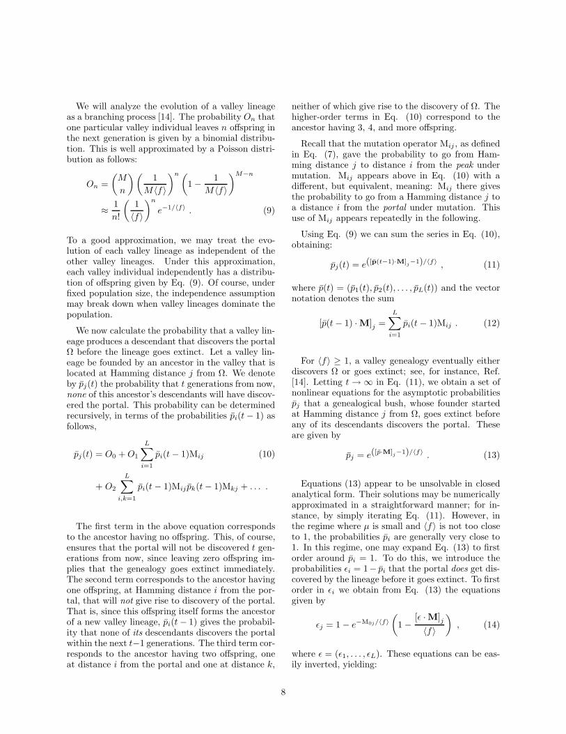
predictions are plotted with solid lines. Each datapoint on the dashed lines was obtained by averagingover 250 runs with equal parameter settings. Thetheoretical predictions are shown as pairs of solidlines, where the lower solid line in each pair showsthe predictions from Eq. (22) and the upper solidline shows Eq. (22) plus the correction term of Eq.(27). Note that for most parameter ranges the dif-ference between the two solid lines is so small as tobe undetectable.

Figures 3(a) and 3(b) show the average barrier

crossing time 〈t〉 as a function of the logarithmlog(σ) of the barrier height. Additionally, both 〈t〉and log(σ) are plotted using a logarithmic scale. Theshapes of the curves correspond to the dependen-cies of log〈t〉 on log(log σ). Portions of curves thatare straight lines thus indicate a scaling of the form〈t〉 ∝ (log σ)s, with s the slope of the straight por-tion. Note that 〈t〉 ranges over 5 orders of magni-tude, from 10 to 106, in both Figs. 3(a) and 3(b).We see that the theory accurately predicts the sim-ulation results for barrier heights that are not toosmall.

µ=0.005M=250

L=10w=4

w=3

w=2

(a)

Log(σ)0.02 0.1 0.2 0.5 1 20.05

<t>

10

106

105

104

103

102

M=250, µ =0.005, w=4

M=250, µ =0.002, w=2

L=7 µM=200, =0.005, w=5

Log(σ)0.02 0.1 0.2 0.5 1 20.05

<t>

10

106

105

104

103

102

(b)

σ=1.19w=3

σ=1.19w=4

σ=1.45w=2

L=7M=250

<t>

10

106

105

104

103

102

0.001 0.002 0.003 0.005 0.007 0.01

(c)

µ2 4 6 8 101 3 5 7 9

w

1

10

106

<t>

105

104

103

102

M=250

L=10,µ=0.015,σ=1.33

L=7,µ=0.01,σ=1.45(d)

FIG. 3. Barrier-crossing times 〈t〉 as a function of barrier height σ, mutation rate µ, and barrier width w, for avariety of parameter settings. The simulation results are plotted using dashed lines. Each point on each dashed lineis an estimate of 〈t〉 averaged over 250 simulation runs. The theoretical predictions are shown as pairs of solid lines:The lower of each pair gives the theoretical predictions of Eq. (22), while the higher has the additional correctionterm of Eq. (27) added. Note that, except for the horizontal axis in Fig. (d), all axes use a logarithmic scale. Generalparameter settings are indicated at the top of each plot, while parameters specific to the different runs are indicatednext to the their lines.

In Fig. 3(a) the theory starts deviating from theexperimental data around log(σ) ≈ 0.06 for the up-per two curves and around log(σ) ≈ 0.15 for thelowest. These values of σ correspond to selective

advantages σ − 1 of the peak of a little over 6and 16 percent, respectively. Notice that the uppertwo experimental curves are almost horizontal forsmall values of σ up to log(σ) ≈ 0.06, after which

11

they trend upwards becoming almost linear. As wewill show below, it turns out that the location ofthis crossover is found at the finite-population error

threshold that separates the entropy-barrier regimefrom the fitness-barrier regime. That is, for the pa-rameters M = 250, µ = 0.005, and L = 10, the crit-ical value σc below which the population dynamicsacts effectively as if there were no fitness peak atall occurs around log(σc) ≈ 0.06. The same phe-nomenon is observed in the two upper curves of Fig.3(b): the crossover occurs around log(σc) ≈ 0.05.Note that the correction terms 〈dt〉 extend the pa-rameter region over which the theory provides ac-curate predictions approximately up to the finite-population error threshold.

Above the error threshold, for values of σ in thefitness-barrier regime, the curves appear nearly lin-ear. This indicates that the barrier crossing timesscale with powers of the logarithm of the barrierheight σ: 〈t〉 ∝ (log σ)s, where s is the line’s slope.Thus, the barrier crossing time increases relativelyslowly as a function of the barrier height. One fur-ther observes that the barrier crossing times are notonly longer for wider barriers (larger values of w),but that the slopes of the curves are larger as well.That is, for large widths w the barrier crossing timeincreases faster as a function of σ than for low valuesof w.

Figure 3(c) shows the barrier crossing time 〈t〉 asa function of the mutation rate µ, for three differ-ent values of the barrier width w and two differentvalues of the barrier height σ. The population sizeis M = 250 and the genotypes length L = 7 for allthree curves. On the logarithmic scales, the curvesagain look approximately linear, indicating that thebarrier crossing time scales as a power law in themutation rate µ: 〈t〉 ∝ µs, where s is the slope.We again see that for wider barriers, the waitingtimes are both larger and vary more rapidly withµ. The theory predicts the simulation results quiteaccurately over the entire range. Only for large mu-tation rates (µ ≈ 0.01) do the theoretical predic-tions with and without the correction term of Eq.(27) differ significantly. In this regime the theoret-ical and experimental values start to differ slightlyas well, although the predictions are still accurate.It is notable in the two lower curve families, withbarrier widths w = 2 and w = 3, that the correc-tion term 〈dt〉 improves the theoretical predictionsfor high mutation rates.

Finally, Fig. 3(d) shows the barrier crossing time

〈t〉 as a function of the barrier width w. Only thebarrier crossing time 〈t〉 is shown on a logarithmicscale, so that any linear dependence indicates an ex-ponential scaling: 〈t〉 ∝ 10sw, where s is the slope.Again, the theory accurately predicts the barriercrossing time. The fact that the curves are not lin-ear and bend downwards shows that 〈t〉 grows moreslowly than exponential with barrier width; althoughit still increases rapidly as a function of w. In fact,we chose large values of the mutation rate µ in theseplots (µ = 0.01 and µ = 0.015) to ensure that thebarrier crossing time is still in a reasonably boundedrange up to large barrier widths. For smaller muta-tion rates, the barrier crossing times become so largeas to make it impossible to perform an adequatenumber of simulation runs. For the case w = 1,the correction term 〈dt〉 leads to an overestimationof 〈t〉. Note, however, that for w = 1 there is ef-fectively no fitness barrier; the portal is a mutantneighbor of the peak genotype and so valley bushesare essentially nonexistent.

In summary, Figs. 3(a)-(d) show that the theoret-ical predictions of Eq. (22), possibly including thecorrection term of Eq. (27), accurately predict theaverage barrier crossing times estimated over a widerange of parameters from simulations of an evolvingpopulation. The theory breaks down, as expected,when the barrier height σ becomes small (σ ≈ 1)and this is illustrated on the left-hand sides of Figs.3(a) and 3(b). In this low-σ regime, which sets insuddenly as a function of σ, 〈t〉 becomes almost inde-pendent of σ. Roughly speaking, the selection pres-sure is too small to keep the population concentratedaround the peak, and the population randomly dif-fuses through the valley until it discovers the portal.In this regime, the barrier is in effect not a fitnessbarrier, but an entropy barrier.

In Sec. IV we will analyze the location of thefinite-population error threshold that separates thefitness and entropy barrier regimes and discuss theentropy-barrier crossing population dynamics. Inthe next subsection, though, we first discuss the scal-ing of the fitness-barrier crossing time 〈t〉 with thedifferent parameters σ, w, µ, and M .

F. Scaling of the Barrier Crossing Time

In Fig. 3 we saw, by varying one parameter at atime, that the barrier crossing time scaled as a powerlaw in the logarithm of the barrier height log(σ),

12

as a power law in mutation rate µ, and somewhatslower than exponential in the barrier width w. An-alytically extracting these scalings from Eq. (22) isquite challenging and incomplete at this time. Em-pirically, though, we found that the barrier crossingtime can be fit quite accurately, in the regime whereσ is not too small (above the error threshold), to ascaling function with the following form

〈t〉 ∝1

w!Mµ

(log(σ)

µ

)w−1

(28)

× [log(σ)]−γ−δ log(µ)

,

where γ and δ are (constant) scaling exponents. Forboth the genotype lengths (L = 7 and L = 10) forwhich we have detailed data, we found that γ ≈ 0.75and δ ≈ 0.1.

This empirical scaling law confirms that, in fact,the barrier crossing time 〈t〉 scales as a power law inboth log(σ) and µ. We see, in particular, that thedependence on the mutation rate µ scales roughly in-versely with µw and the dependence on log(σ) scales

roughly as [log(σ)]w−2. Furthermore, we see that 〈t〉scales as ecw/w!, with c a constant, when only thebarrier width w is varied. The scaling with w is thusby far the most rapid and therefore dominant scaling.That is, widening the barrier increases the waitingtime 〈t〉 much more than increasing the height of thebarrier or decreasing the mutation rate.

These empirically observed scaling behaviors canbe elucidated using a simple analytical argument.To this end we employ several simplifications. First,we assume that the major contributions to the prob-ability of barrier crossing come from terms with theminimal number of mutations. That is, for barri-ers of width w, at least w mutations must occur ina peak individual in order to discover the portal.Thus, we assume that contributions from “paths”between peak and portal that involve more thanw mutations are negligible. This for instance im-plies that we neglect the contributions from lineagesfounded at Hamming distances w through L fromΩ. Furthermore, we assume that valley lineages areunlikely to be founded more than 1 mutation awayfrom the peak. Putting these together, the domi-nant contribution to the barrier crossing probabilitycomes from lineages that are founded at a Hammingdistance w − 1 from the portal. Note that if weset PΠ = 1 for simplicity, each generation approxi-mately

wµM

1 − µ(29)

such lineages are founded.

We will now estimate the probability that a lin-eage, starting at Hamming distance w − 1 from theportal, discovers the portal exactly t generations af-ter its founding. We approximate the valley genealo-gies by assuming that each valley individual can onlyhave zero or one offspring each generation. This im-plies that a valley lineage consists of a single line ofindividuals; i.e., lineages do not branch. The proba-bility that such a lineage persists for at least t timesteps is 1/〈f〉

t. At t = 0, the lineage has w−1 bits set

incorrectly, and L−w+1 bits set correctly. In orderfor the lineage to discover the portal exactly at timet, it will have to mutate its bits such that, at time tand for the first time, the w− 1 “incorrect” bits willall have been flipped to the correct state and all theL − w + 1 correct bits are left undisturbed. Thus,between time 0 and t, the w − 1 incorrect bits haveto be mutated exactly once, while the correct bitshave been undisturbed. Since we are calculating theprobability for the portal to be discovered exactly attime t, one of the w − 1 bits has to flip at time t,while the other w − 2 might flip at any prior time.This gives (w − 1) tw−2 possibilities for contributingflips. All other bits have to remain unflipped for alltime steps.

Thus, the probability P findt that a lineage finds the

portal exactly at time t is approximately given by:

P findt = (w − 1) tw−2

× µw−1(1 − µ)Lt−w+1

(1

〈f〉

)t

, (30)

where the last factor gives the probability that thelineage survives until time t. Using Eq. (2) andsumming Eq. (30) over t we find:

P find =∞∑

t=0

P findt

= (w − 1)

(µ

1 − µ

)w−1 ∞∑

t=0

tw−2

(1

σ

)t

= (w − 1)

(µ

1 − µ

)w−1

Li2−w

(1

σ

)

, (31)

where Lin(x) is the poly-logarithm function: essen-tially defined by the sum in the second line above.It is more insightful to approximate the sum with anintegral. We then obtain

13

P find =

(µ

1 − µ

)w−1 ∫ ∞

0

(w − 1) tw−2e− log(σ)tdt

= (w − 1)!

(µ

log(σ)(1 − µ)

)w−1

. (32)

Recall that the rate at which lineages at Hammingdistance w−1 are being created is wµM/(1−µ). Us-ing this and noting that the barrier crossing time isinversely proportional to P find, we obtain a scalingof the form

〈t〉 ∝1

w!Mµ

(log(σ)

µ

)w−1

, (33)

where we have neglected the factor (1 − µ)w ≈ 1.The scaling relation of Eq. (33) recovers most of theempirically determined scaling behavior in Eq. (28).

The dominant scaling with µ and log(σ) can beunderstood as follows. The average time that alineage spends in the valley before going extinct isroughly 1/ log(σ). Thus, µ/ log(σ) gives the averagenumber of mutations that a lineage in the valley un-dergoes before it goes extinct. Since this number isgenerally much smaller than 1, it can be interpretedas the probability of having a single mutation in avalley lineage. The probability of having w − 1 mu-tations is then of course (µ/ log(σ))w−1. There isan additional factor 1/µ from the rate at which val-ley lineages are being created at Hamming distancew − 1. Ref. [31] also argues, along somewhat differ-ent lines, that the barrier crossing time should have apower-law dependence on mutation rate: 〈t〉 ∝ µ−w.

The correction factors—those with scaling expo-nents γ and δ in Eq. (28)— probably arise from thefact that lineages are not simple unbranching linesof descendants, as we have assumed, but are morecomplicated tree-like genealogies.

The factor w! in Eq. (33) counts the number ofdistinct paths of minimal length between the peakand the portal. Curiously, it appears from the scal-ing formulas that when w gets very large, the bar-rier crossing time starts to decrease again. Apply-ing Stirling’s approximation to the factorial func-tion in Eq. (33) indicates that 〈t〉 has a maximumaround wµ = log(σ). Although this may initiallyseem strange, it does make sense, since as we willnow argue, fitness barriers for which wµ > log(σ)do not exist.

If there are w! independent paths between peakand portal, this implies that there are w indepen-

dent directions from the peak into the valley. Inother words, at least w bits of the peak genotypecan undergo deleterious mutations. As we will seein Sec. IV below, the error threshold at which peakindividuals becomes unstable in the population oc-curs near

σ(1 − µ)L = 1 . (34)

To first order in µ, this is equivalent to log(σ) = Lµ.That is, if Lµ > log(σ), peak individuals will be lostfrom the population, and the population will startdiffusing randomly through genotype space. Obvi-ously, the genotype length has to be longer than thebarrier width L > w. Therefore, wµ > log(σ) im-plies that the genotype length L is so large that it isimpossible to stabilize the peak individuals. In otherwords, fitness barriers with wµ > log(σ) simply donot exist.

Finally, it should be noted that as log(σ) → ∞,the barrier crossing time goes to a finite asymptoteand not to infinity. Since valley lineages have proba-bility zero to reproduce in this limit, the asymptoticbarrier crossing time is given by the (finite) waitingtime for a “long jump” in which a peak individualundergoes w mutations at once.

The main consequence of the scaling relations justderived, is that if the population is located on a fit-ness “plateau” in genotype space, surrounded by dif-ferent valleys on all sides, then it will most likely es-cape from the plateau via the valley with the small-est width and not via the valley path with the small-est depth. One concludes that high barriers can bepassed relatively easily, as long as they are narrow;while wide barriers take a very long time to cross,even if they are shallow.

We should emphasize that this situation is verydifferent from the scaling of barrier crossing timesgenerally encountered in physics or, for that mat-ter, in evolutionary models that literally interpretthe “landscape” metaphor as leading to stochasticgradient dynamics on a fitness “potential”. In thesesettings, the system’s state space has an energy func-tion defined on it that acts as a potential field. In theabsence of any noise, the system is assumed to followthe gradient (downward) of the energy “landscape”.In the presence of noise, the system can deviate fromits gradient path, but movement against the gradi-ent is unlikely in proportion to its deviation fromthe local gradient. The barrier crossing times thendepend mainly on the barrier height, and they scaleexponentially with this barrier height [12].

14

For example, imagine an energy barrier that con-sists of a steep slope upwards, followed by a longplateau and then a steep slope leading downward onthe other side. The initial steep ascent from the val-ley onto the plateau is very unlikely since it involvesmoving against a steep gradient. However, after thisunlikely step has been established, the system cancross the long plateau to the other side relativelyeasily, since it does not involve moving against anenergy gradient. Thus, the width of the energy bar-rier is almost immaterial, while the barrier height isthe defining impediment, since it determines the ex-tent to which movement against the gradient mustoccur.

The situation is entirely different for fitness “land-scapes” in which an evolving population moves. Foran evolving population, making a large jump in fit-ness is not unlikely at all. One mutation in one indi-vidual can do the trick. However, since some individ-uals remain at the peak, the individuals in the valleyare continuously in competition with these higher-fitness peak individuals. An absolute fitness scale isset by these peak individuals. It is therefore survivalat low fitness—compared to the most-fit individualsin the population—for an extended period of timethat is unlikely. And this is why the time it takesto move across the plateau is the key parameter—which, of course, is controlled by the barrier width.

The preceding discussion should make it clear,once again, that this analogy—between a populationevolving over a fitness “landscape” and a physicalsystem moving over its energy “landscape” in statespace—is problematic: at best it may lead one to thewrong intuitions; at worst the basic physical resultssimply do not describe evolutionary behavior.

IV. THE ENTROPY BARRIER REGIME

Figures 3(a) and 3(b) showed that below a criticalbarrier height σc, where the dashed lines began torun horizontally, the barrier crossing time becameeffectively independent of σ. We also saw that thetheory breaks down for σ < σc. In this regime, allpeak individuals are quickly lost and the populationdiffuses through the valley until the portal is discov-ered. The theoretical calculations, in contrast, as-sumed the population was located at the peak andthat short lineages were continuously spawned in thevalley. It is no surprise then that the predictionsbreak down in this regime. Since the population

dynamics is dominated by diffusing through the val-ley’s fitness-neutral volume, we refer to this as theentropy-barrier regime. Before discussing the barriercrossing times in this entropic regime, we first esti-mate the error threshold’s location σc as a functionof µ, M , and L.

A. Error Thresholds

As a first, population-size independent approxi-mation one might guess that the error threshold oc-curs when the average number of peak-offspring pro-duced by a single peak individual in a population ofvalley individuals is 1. From Eq. (2) this leads toan estimated critical barrier height σc of

σc = (1 − µ)−L . (35)

This equation is the standard error-threshold resultin molecular quasispecies theory [6,7]. For the pa-rameters L = 10 and µ = 0.005 of Fig. 3(a),this leads to log(σc) ≈ 0.05, or σc ≈ 1.05. Asseen from the figure, though, the entropic regimeextends to somewhat higher peak fitness; as faras log(σ) ≈ 0.06. This deviation is due to finite-population sampling effects and to neglecting backmutations, which become important as the errorthreshold is approached.

For finite populations, the error threshold can bedefined most naturally as those parameter values forwhich the mean proportion PΠ of peak individualsequals the variance, due to finite population fluctu-ations, in PΠ. That is, the criterion for reaching theerror threshold is

(PΠ)2 = Var(PΠ) . (36)

The intuition behind this definition is as follows:Since the proportion of peak individuals fluctuates,eventually a large fluctuation will occur that leads tothe loss of all peak individuals. As was shown in Ref.[30], however, the waiting time for such a destabi-lization to occur increases exponentially with the ra-tio (PΠ)2/Var(PΠ). Only when (PΠ)2 < Var(PΠ) dosuch destabilizations occur relatively frequently. For(PΠ)2 > Var(PΠ) the fluctuations are small enoughso that the proportion of peak individuals typicallydoes not vanish. Therefore, it is natural to use Eq.(36) to delineate the regimes with “unstable” and“stable” peak populations and so to distinguish be-tween the fitness-barrier and entropy-barrier regimesin the population dynamics.

15

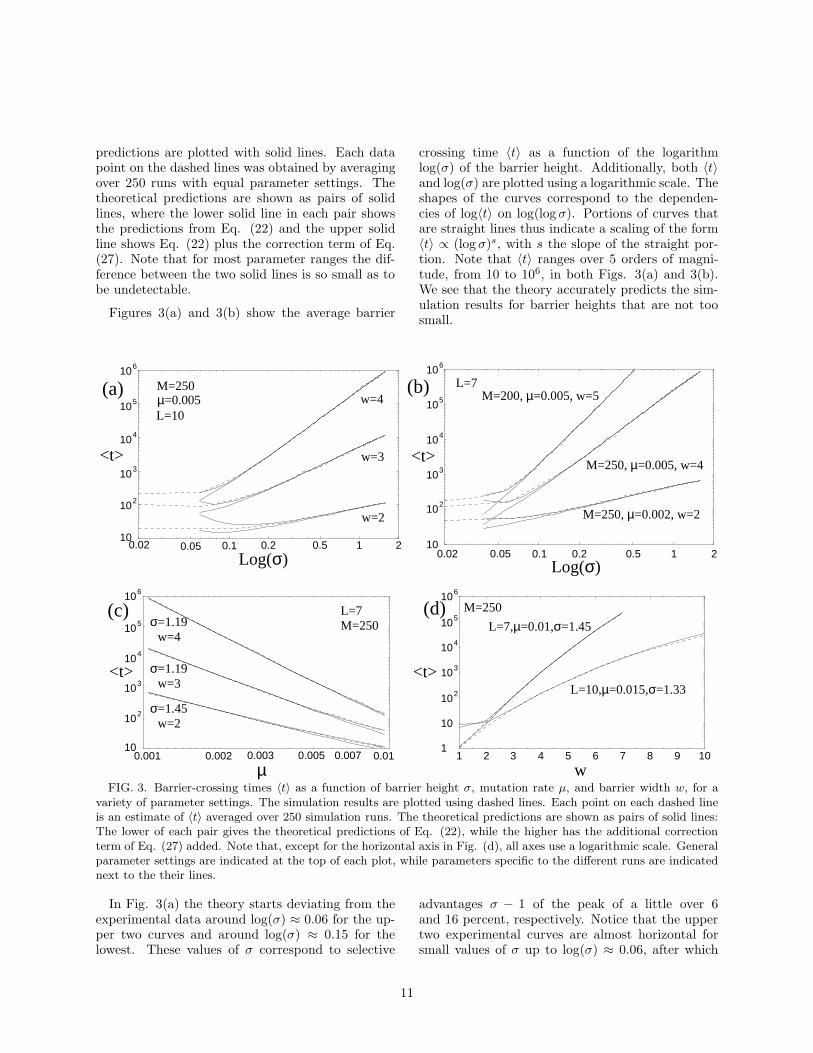
Finite-population error thresholds may also be de-fined in alternative ways; cf. Ref. [24]. Typically,one finds that, although the conceptual motivationsdiffer, the quantitative parameter values for whichthe different error thresholds occur are quite simi-lar.

The variance Var(PΠ) can be most easily cal-culated using diffusion-equation methods. For anintroduction to these techniques in the context ofmathematical population genetics, see for instanceRef. [18]. To begin, we assume that, due to sam-pling fluctuations, at some particular time t the ac-tual proportion of peak individuals is not PΠ butinstead is P (t) = PΠ + x(t). That is, the proportionP (t) of individuals on the peak deviates x(t) fromits equilibrium value PΠ. We focus on the dynamicsof the deviation x(t). At the next generation, theexpected deviation 〈x(t + 1)〉 is

〈x(t + 1)〉 =x(t)

〈f〉. (37)

Thus, the expected change 〈δx〉 in the deviation isgiven by

〈δx〉 =1 − 〈f〉

〈f〉x ≡ −γ x , (38)

where we have defined γ by the last equality. γmeasures the average rate at which fluctuationsaround the quasispecies equilibrium distribution aredamped. The second moment 〈(δx)

2〉 of the change

δx is approximately given by the variance of thebinomial-sampling distribution. One finds that

〈(δx)2〉 =

1

M

(

PΠ +x

〈f〉

)(

1 − PΠ −x

〈f〉

)

. (39)

A Fokker-Planck diffusion equation approxima-tion determines the temporal evolution of distribu-tion Pr(x, t) of x(t) via

∂

∂tPr(x, t) = −

∂

∂x〈δx〉Pr(x, t)

+1

2

∂2

∂x2〈(δx)2〉Pr(x, t) , (40)

where 〈δx〉 from Eq. (38) gives the drift term and〈(δx)2〉 from Eq. (39) the diffusion term. Solvingfor the limit distribution Pr(x) for x yields

Pr(x) = C

(

PΠ +x

〈f〉

)2M〈f〉(〈f〉−1)PΠ

×

(

1 − PΠ −x

〈f〉

)2M〈f〉(〈f〉−1)(1−PΠ)

. (41)

Here C is a normalization constant that ensuresPr(x) is normalized on the interval x ∈ [−PΠ, 1 −PΠ]. If we expand the fluctuations to second-orderaround x = 0, the distribution becomes a Gaussiangiven by

Pr(x) = Ce− Mγ

PΠ(1−PΠ)x2

, (42)

where C is again a normalization constant. Fromthis distribution of fluctuations one directly readsoff the variance Var(PΠ), finding that

Var(PΠ) =PΠ(1 − PΠ)

2Mγ

=〈f〉 (σ − 〈f〉)

2M(σ − 1)2, (43)

where we used Eqs. (3) and (38) to arrive at the lastline.

As noted before, we define the finite-populationerror threshold by those parameter values for which(PΠ)2 = Var(PΠ). Using Eq. (43) leads to the error-threshold parameter constraints given by

2M(〈f〉 − 1)2

〈f〉(σ − 〈f〉)= 1. (44)

If we substitute the parameter values µ = 0.005,M = 250, and L = 10 of Fig. 3(a) and useEq. (2) for 〈f〉, we find the error threshold atlog(σc) ≈ 0.059. This agrees quite well with the lo-cation at which the experimental curves start bend-ing upwards with increasing peak height.

B. The “Landscape” Regime

As we have pointed out previously, the scaling re-lations derived in Sec. III F contrast strongly withthose based on “landscape” models in which the pop-ulation as a whole diffuses through the fitness land-scape [20,22]. For those models, the barrier cross-ing time scales exponentially with population sizeand barrier height. It turns out that this scaling

16

behavior—appropriate to the “landscape” regime—can be reconciled with the scaling formulas derivedin Sec. III F by closer inspection of Eq. (44).

As noted above, the average destabilization time

for a fluctuation to occur that makes all peak indi-viduals disappear from the population scales expo-nentially in the ratio Var(PΠ)/(PΠ)2 given by Eq.(44). Thus, Eq. (44) shows that this destabilizationtime increases exponentially with population size.For cases where 〈f〉 ≫ 1 and for reasonable popu-lation sizes, the destabilization time is so large thatthe barrier crossing time is determined by how longit takes a rare mutant to cross the fitness valley.

Close to the finite-population error-threshold(〈f〉 ≈ 1), however, it might be the case that thetime to create such a rare sequence of mutants is longin comparison to the destabilization time. In this sit-uation, the barrier crossing time is essentially givenby the destabilization time: As soon as all peak indi-viduals are lost, the population diffuses through thevalley and quickly discovers the portal. Thus, in thevery restricted “landscape” parameter regime justaround the error-threshold, the barrier crossing timeis determined by the destabilization time and does

scale exponentially with population size and barrierheight.

Beyond the error threshold—that is, for smallerpopulations, larger mutation rates, smaller barrierheights, or longer genotypes—the peak readily be-comes unoccupied. In this regime, the barrier cross-ing time becomes almost independent of barrierheight σ. The barrier to be crossed is then no longera fitness barrier. Instead, it has become an entropybarrier. The population must search through almostall of the valley until the portal is discovered. Thus,only for parameters near the boundary between thefitness and entropic regime does the barrier cross-ing time scale in accordance with the “landscape”models.

C. Time Scales in the Entropic Regime

The population dynamics in the entropic regimebeyond the error threshold is modeled most directlyby considering an entirely flat (constant) fitnessfunction; in particular, one in which all genotypeshave fitness 1 and containing a single portal Ω. Thepopulation starts out concentrated on a genotypeat Hamming distance w from Ω and evolves under

selection and mutation until the portal genotype isdiscovered for the first time. Denote this averageentropy-barrier crossing time by τ .

The calculation of the entropy-barrier crossingtime appears less analytically tractable than the cal-culation of the fitness-barrier crossing time. Themain difficulty arises from the sampling of individu-als at each generation, combined with the global con-straint of a fixed population size. Due to this sam-pling dynamics, subtle genetic correlations emergebetween the individuals. Although some of the as-pects of the correlation statistics have been derivedanalytically [5], the entropy-barrier crossing time τdepends in a complicated, and not yet well under-stood, way on these correlations. We will discuss thedifficulties with calculating entropic barrier crossingtime by deriving several simple approximations anddiscussing why they fail to provide accurate quanti-tative predictions.

First, one can approximate the neutral evolutionjust defined by assuming that each individual in thepopulation has exactly one offspring. In this case,the population effectively consists of M independentrandom walkers that diffuse through genotype space.Since each individual has only one offspring one canidentify its genealogy with a single evolving genotypethat mutates each bit with probability µ at each gen-eration. Since µL ≪ 1 in general, this genotype ef-fectively performs a random walk in the hypercube,where random walk steps are made at a rate of onestep per 1/(Lµ) generations on average.

The average time τ1 a single random walker takesto discover Ω is given by:

τ1 =L∑

i=1

(I− M)−1iw , (45)

where the matrix indices run from Hamming dis-tance 1 through L. τ1 determines an upper boundfor the entire population’s barrier crossing time. Forparameter settings in the fixation regime, whereMLµ ≪ 1, sampling fluctuations cause the popula-tion to converge onto M copies of a single genotype.As is well known from the theory of neutral evolution[19], this set of identical genotypes performs a ran-dom walk through the genotype space at the samerate as a single individual. Thus, in this limit, τ1

gives a reasonable prediction for the entropy-barriercrossing time. However, for Fig. 3(a)’s parametersettings (M = 250, µ = 0.005, and L = 10) that giveMLµ = 12.5, we find that τ1 ≈ 23000, almost inde-

17

pendent of valley width w. Of course, this grosslyoverestimates the observed barrier crossing times,which vary from 〈t〉 ≈ 25 for w = 2 to 〈t〉 ≈ 227for w = 4.

For M independent random walkers, one mightsimply assume that the waiting time would beroughly a factor M slower, i.e. τM = τ1/M . Unfor-tunately, this leads to τM ≈ 93 which overestimatesthe observed time for w = 2 and underestimates 〈t〉for w = 4.

The precise probability pw(t), that none of M in-dependent random walkers starting at a Hammingdistance w have found the portal by time t, is givenby:

pw(t) =

(L∑

i=1

Mtiw

)M

. (46)

From this, one estimates the average entropy-barriercrossing time τ to be:

τM =

∞∑

t=1

t [pw(t − 1) − pw(t)]

=

∞∑

t=0

pw(t) . (47)

For Fig. 3(a)’s parameters, Eq. (47) gives τ ≈ 15,58, and 117 for barrier widths w = 2, 3, and 4,respectively. These values underestimate each ob-served waiting time by almost a factor of 2. Appar-ently, sampling fluctuations cause the population toexplore the genotype space less rapidly than inde-

pendent random walkers do. As already noted above,the reason for this is that sampling convergence leadsdifferent individuals to evolve genetic correlations tosome degree.

One way to think about this is to investigate ge-nealogies. Ref. [5] showed that the probability Pr(t)for two randomly chosen individuals in the currentpopulation to have had a common ancestor less thant generations ago is approximately given by

Pr(t) ≈ 1 − e−t/M . (48)

This means that, on average, a pair of individualshas only undergone MLµ mutations each since thetime t ≈ M they descended from a common an-cestor. When Mµ is not much larger than 1, thisimplies that two individuals are more strongly cor-related genetically than random genotypes. Due to

this, it is easy to see, at least qualitatively, that theentropy-barrier crossing time is longer than that pre-dicted for independent random walkers. The corre-lation, or clustering, of individuals in genotype spaceleads the population to explore the valley’s neutralvolume at a slower rate. Thus, the predictions ob-tained by assuming M random walkers, as given byEqs. (46) and (47), are lower bounds to the actualwaiting times.

It turns out that the upper (Eq. (45)) and lower(Eq. (47)) estimates do not tightly bound the ac-tual waiting times 〈t〉. They may differ by severalorders of magnitude. Fortunately, the lower boundobtained from Eqs. (46) and (47) typically producesreasonable order-of-magnitude estimates for param-eter regimes in which MLµ > 1. This order-of-magnitude estimate gives the following scaling re-lation for the entropy-barrier crossing time

τ ≈2L

MLµ. (49)

D. Anomalous Scaling

The order-of-magnitude estimate given by Eq.(49) predicts that the the entropy-barrier crossingtime τ scales inversely with both µ and M . Thisscaling is, of course, exactly one’s intuitive expec-tation: the rate at which the genotype space is ex-plored is proportional to both mutation rate µ andpopulation size M . M individuals cover M times asmuch genotypic “ground” as one individual. Individ-uals that “move” twice as fast, cover twice as muchground as well. And so, the waiting time should beinversely proportional to both M and µ, which setthe exploration rate.

In light of this, it is interesting that data from sim-ulations shows that the entropy-barrier crossing timeτ scales as a power law in both µ and M , but not

with exponents equal to −1, as the preceding sim-ple argument suggests. To be clearer on this point,Fig. 4 illustrates the observed scaling behavior ofthe entropy-barrier crossing time as a function of Mand µ.

The solid lines plot the data obtained from simula-tions while the dashed lines show scaling (power-law)functions that were fitted to the experimental data.All axes use logarithmic scales. All simulations were

18

performed with genotypes of length L = 10 bits. Inall of the runs, at time t = 0 all individuals start atHamming distance w = 5 from the portal. Figure4(a) shows τ ’s dependence on M for three differ-ent values of µ. The approximately straight linesshow that the entropy-barrier crossing time dependsroughly as a power law on the population size M :

τ ∝1

Mα. (50)

Of course, the scaling exponent α may itself dependon µ.

Similarly, Fig. 4(b) shows the dependence of τ onµ for two different values of M . In this case too, thecurves appear well approximated by a straight line,indicating that for fixed M the dependence on µ isroughly given by

τ ∝1

µβ, (51)

where β may again depend on the population size M .In Table I the exponents of the estimated dashedlines in Figs. 4(a) and 4(b) are given, along withtheir estimated errors.

µ 0.002 0.005 0.008

α 0.740 ± 0.01 0.744 ± 0.02 0.761 ± 0.03

M 50 250

β 1.292 ± 0.008 1.365 ± 0.014

TABLE I. Estimated exponents α and β as defined byEqs. (50) and (51).

1 10 100 1000 1000010

100

1000

10000

100000

µ=0.002

µ=0.005

µ=0.008

M

τ

0.001 0.0110

100

1000

10000

100000

µ

τ M=250

M=50

(a) (b)

FIG. 4. Entropy-barrier crossing time τ as a function of population size M and mutation rate µ. The solid linesare data obtained from simulations, while the dashed lines show the estimated scaling functions. All experimentswere done with genotypes of length L = 10 and a barrier width of w = 5. All axes are shown on logarithmic scales.In Fig. (a) τ is shown as a function of population size M for three values of the mutation rate µ. In Fig. (b) τ isshown as a function of the mutation rate µ for two values of population size M . The approximately straight linesshow that τ scales as a power law in M when µ is kept constant and, vice versa, as a power law in µ when M is keptconstant. Table I lists the estimated exponents for the power laws. These were used to plot the dashed lines.

The values of the exponents α for different µ and βfor different M are very close to each other; α ≈ 3/4and β ≈ 4/3. It is clear, however, that they are notconstants: α does depend on µ and β on M . Notethat the estimates for α are all below 1, while thosefor β are above 1. Thus, doubling the populationsize decreases τ by less than a factor of two, whiledoubling the mutation rate decreases τ with more

than a factor of two. Intuitively, what is happen-ing is that, due to the clustering in the population,doubling the population size does not lead to a dou-bling of the exploration rate. That is, some of the“added” members in the larger population will sim-ply occur at genotypes where other members of thepopulation are already located. Thus, they do notcontribute to additional novel exploration. In con-

19

trast, doubling the mutation rate not only doublesthe rate of movement (diffusion) of individuals inthe population, it additionally decreases the cluster-ing and so reduces genetic correlations. Due to thecombination of these two effects, the entropy-barriercrossing time decreases more than a factor two.

Of course, one would like to predict these anoma-lous exponents. In principle, they should be calcu-lable from knowledge of the clustering structure ofthe population at different values of M and µ. Forexample, if we view the population as a blob or col-lection of blobs in genotype space, one would liketo know how many distinct genotypes, on average,are neighboring one or more individuals of the pop-ulation. Roughly speaking, we would like to knowthe average “surface area” of the population in geno-type space. Knowledge of this statistic would thensupply us with the average probability that a mu-tation leads to a genotype not currently present inthe population. This, in turn, quantifies the popula-tion’s rate of exploring novel genotypes, while takinginto account genetic correlations. Although severalstatistics of these genotype blobs were calculated inRef. [5], we have at present not been able to adaptthese results to infer the necessary type of statisticsjust outlined. The analytical prediction of the scal-ing exponents α and β thus awaits further progress.For the present, we will use our order-of-magnitudeestimate in Eq. (49) to compare the entropy-barriercrossing time with the fitness-barrier crossing times.

In summary, we analyzed the fitness- and entropy-barrier crossing times for the simplest (single peak)landscapes in which both types of barrier occur. Ourresults are summarized by the scaling relations ofEqs. (28) and (49). In the following sections, weapply the preceding analysis to more complicatedfitness functions that contain multiple fitness andentropy barriers.

V. TRAVERSING COMPLEX FITNESS

FUNCTIONS

Up to this point, to make analytical progress wefocused on fitness functions that were intentionallysimple: a single portal and a single peak in genotypespace. Despite this, the analysis of barrier crossingtimes just developed can be extended with relativeease to more complicated evolutionary processes. Toillustrate this extension of the theory, we now intro-duce a class of more complicated fitness functions

that contain multiple fitness and entropy barriers oftunable width and height. That is, in this class offitness functions, the population may have to crossboth a fitness and entropy barrier to escape fromits metastable state. Since the relative sizes of boththese types of barriers can be tuned, we can explic-itly compare the time scales for crossing fitness andentropy barriers within the same evolutionary pro-cess.

A. The Royal Staircase with Ditches

The class of fitness functions which we call theRoyal Staircase with Ditches is closely related tothe Royal Staircase and Royal Road fitness functionsthat we have analyzed previously [4,27–30]. Thosefitness functions did not contain fitness barriers butinstead consisted of a series of entropy barriers. Thefunction class of Royal Staircases with Ditches gen-eralizes these fitness functions and is defined as fol-lows:

• Genotypes consist of bit sequences of lengthL, interpreted as N blocks of K bits each:L = NK.

• The blocks are ordered, not in the sense thatthey correspond to particular positions in thegenotype, but only in the sense that they areindexed 1 through N . Note that since ourevolutionary process does not include recom-bination, the population dynamics is invariantunder arbitrary permutations of a genotype’sbits. For convenience, we order the blocks fromleft to right in the genotypes. That is, bits 1through K belong to the first block, bits K +1through 2K belong to the second block, and soon.

• The 2K possible configurations of the K-bitblocks each are divided into three classes.

1. Type-A blocks consist of a configurationwith K ones:

A = 111 · · ·111︸ ︷︷ ︸

K

. (52)

2. Type-B blocks consist of a configurationwith K − w ones and w zeros:

B = 111 · · ·111︸ ︷︷ ︸

K−w

w︷ ︸︸ ︷

000 · · ·000 . (53)

20

As will become clear, the parameter wcontrols the width of the barriers.

3. All other 2K − 2 configurations are de-noted as Type-∗ blocks.

• A genotype s with blocks 1 through n − 2 oftype B and block n−1 of type A receives fitnessf(s) = n. These genotypes have the structure:

BB · · ·BB︸ ︷︷ ︸

n−2

A

N−n+1︷ ︸︸ ︷∗ ∗ · · · ∗ ∗ . (54)

Note that the configurations of blocks nthrough N are immaterial (denoted ∗) whenthe first n− 1 blocks occur in the above geno-type configuration.

• Genotypes s with blocks 1 through n − 2 oftype B , block n − 1 of type ∗, and block nof type A receive fitness f(s) = n − h. Thesegenotypes have the structure:

BB · · ·BB︸ ︷︷ ︸

n−2

∗A

N−n︷ ︸︸ ︷∗ ∗ · · · ∗ ∗ , (55)

Again, the configurations of blocks n + 1through N are immaterial. The parameter hcontrols the height of the fitness barrier.

The Royal Staircase fitness functions that we stud-ied in Refs. [28] and [27] are a special case (w = 0)of the Royal Staircase with Ditches class of fitnessfunctions. For the special case w = 0 there are nofitness barriers and a genotype has fitness n whenthe first n − 1 blocks are A = B (all 1s) types andthe nth block is set to any of the 2K − 1 other con-figurations.

Setting w = 1 produces a somewhat degeneratecase that we will not consider.

For values of w ≥ 2, there is a genuine fitness bar-rier of width w bits. For instance, consider the casewhere, at some point in time, the highest fitness inthe population is f = 4. This corresponds to geno-types that have first and second blocks of type Band a third block of type A. In this case, a portal

genotype Ωn, corresponding to a fitness of 5, is ob-tained when the fourth block is set to type A and thethird block is changed from type A to type B. Geno-types with fitness 4 can mutate their fourth block,until it becomes type A, without changing their fit-ness. That is, the fourth block may be changed

into type A along a neutral path and setting the 4thblock correctly corresponds to crossing an entropybarrier. However, after that, the third block needsto be changed from type A to type B. All interme-diate type ∗ blocks give genotypes a reduced fitnessof f = 4 − h. We call these ditch genotypes, sincethey are located in a lower-fitness region in genotypespace that separates genotypes with fitness 4 fromgenotypes with fitness 5.

B. Evolutionary Dynamics

We evolve populations on the Royal Staircase withDitches under a simple selection and mutation dy-namics similar to the one outlined in Sec. II. Thisconsists of the following steps.

1. At time t = 0 a population of M ran-dom binary-allele genotypes (bit sequences) oflength L is created. These M individuals con-stitute the initial population.

2. The fitness of all M individuals is determined,using the function defined in the previous sec-tion.

3. M individuals are sampled from the popu-lation, with replacement, and with probabil-ity proportional to their fitness. That is, thepopulation undergoes fitness-proportional se-lection in discrete generations.

4. Each bit in each of the M selected individu-als is mutated with a probability µ. The Mindividuals thus obtained form the new gener-ation.

5. The procedure is repeated from Step 2.

We evolve the population according to the abovedynamics until genotypes of optimal fitness havebeen discovered and the population appears to havereached a stable average fitness. During each run, weestimate a number of statistics—such as, the aver-age time until individuals of a certain fitness appearfor the first time.

21

C. Observed Population Dynamics

The population dynamics under Royal Staircasewith Ditches functions is qualitatively very similarto that under the Royal Road and Royal Staircasefitness functions. Samples of this typical behaviorare shown in Figs. 5(a)-(d). The plots there show

the average 〈f〉 (lower, solid lines) and best (up-per, dashed lines) fitnesses in the population overtime for four single runs with four different param-eter settings. The parameter settings for each runare indicated above each figure, except for the bar-rier widths w and barrier heights h that were used.All runs used barriers of widths w = 2 and heightsh = 1.

FIG. 5. Four runs of the Royal Road with Ditches population dynamics with four different parameter settings.The upper dashed lines plot best fitness and the lower solid lines, average fitness 〈f〉 in the population as a functionof time, measured in generations. The parameter settings for each run are indicated above each figure. All fitnessfunctions have barriers with a width of w = 2 and a height of h = 1. The values of the average fitnesses were obtainedby taking a running average over 10 generations. This reduces the relatively large fluctuations in average fitnessbetween successive generations.

The qualitative dynamics follows the typical alter-nation of long periods of stasis (epochs) in the aver-age population fitness and short bursts of innovation

to higher average fitness; a class of evolutionary dy-

namics that we call epochal evolution [29]. At thebeginning of a run the average and best fitness arelow. This simply reflects the fact that high-fitnessgenotypes are very rare in genotype space and there-

22

fore do not occur in an initial random population.A balance is quickly established between selectionand mutation that leads to a roughly constant aver-age fitness in the population. This period of stasiswe call an epoch. After some time, a mutant maycross the fitness barrier and discover a portal, i.e., ahigher-fitness genotype. Relatively frequently, thishigh-fitness mutant is lost through sampling fluc-tuations or deleterious mutations. Such events areseen as isolated spikes in the best fitness in Fig. 5.Eventually, one of these beneficial mutants spreadsthrough the population—an innovation occurs. Atthis point the average fitness increases, until a newequilibrium between selection and mutation is estab-lished.

Although many properties of epochal evolutioncan be treated analytically [30], here we will focussolely on the epoch times. These are the averagetimes between the start of a given epoch and thestart of the next. Average epoch times can be ob-tained from simulation data by tracing backward intime the behavior of the population’s best fitness.The population dynamics runs until genotypes of thehighest possible fitness N +1 have established them-selves in the population for an extended period oftime. (For certain parameter settings—specifically,those beyond the error threshold—genotypes withthe highest fitness may not stabilize in the popula-tion at all. For such parameter settings, an epochtime can be effectively infinite. We will not considersuch parameter settings explicitly here.) From therewe trace backwards the last time tn that fitness nwas the highest in the population, for all values ofn. The differences tn − tn−1 give the epoch timesτn. Some fitness levels may not occur during a run.For instance, in Fig. 5(a) fitness f = 1 never oc-curs, since the population starts out with genotypesof fitness 2. The epoch time τ1 is therefore 0 forthis particular run. Average epoch times are thenestimated by averaging the epoch time τn over anensemble of runs. In the following we calculate ana-lytical approximations to these epoch times τn, usingthe results from the preceding development.

D. Epoch Quasispecies and The Statistical

Dynamics Approach

In order to approximate epoch times analytically,we need to determine the average proportion ofthe population at highest fitness during each epoch.This is the equivalent of PΠ in Sec. III. From this

we can estimate the rate of creation of genealogies inthe ditch between the neutral networks of two succes-sive epochs. Then we need to calculate the averagepopulation fitness during each epoch to determinethe average life time of these ditch genealogies. Forthe fitness functions studied in the Sec. III thesequantities were relatively straightforward to calcu-late. There, individuals were either on the peak orin the valley, at a certain distance from the portal.For the Royal Staircase with Ditches fitness func-tions the situation is more complicated.

In principle, one can calculate the current equiv-alent of PΠ by representing the population as a dis-tribution of genotypes and calculating metastablegenotype distributions for each epoch. This is typi-cally done in population genetics models [9] and inthe standard quasispecies models of molecular evo-lution [7]. However, since genotype spaces are typ-ically very large, an analytical treatment that ex-plicitly takes into account finite-population effects isgenerally infeasible within this genotypic representa-tion. To address this problem, we introduced an al-ternative approach that we call statistical dynamics

[4,29,30]. There one chooses a relatively small num-ber of macroscopic variables with which to describethe population at any given time. Other degreesof freedom are then averaged out using a maximum

entropy method similar to the Gibbs method fromstatistical mechanics. We will use this approach be-low and simply refer the reader to Refs. [4] and [30]for more extensive treatment of statistical dynam-ics and a discussion of the relation of this approachto standard quasispecies theory, mathematical pop-ulation genetics, and other theories from the field ofevolutionary computation [25].

We represent the population state at any pointin time by a fitness distribution. That is, insteadof describing the population by the relative frequen-cies of all genotypes in the population, we describeit by the relative frequencies of different fitness val-ues. Of course, a given fitness distribution does notuniquely specify a population of genotypes. In or-der to construct the dynamics on the level of fitnessdistributions, we must “average out” the additionalgenotypic degrees of freedom somehow. We do thisby assuming, at each generation, a maximum en-tropy distribution of genotypes given the distribu-tion of fitness. In the Royal Staircase with Ditchesfitness functions, this translates into assuming thateach string with a given fitness f is equally likelyto be any of the genotypes with fitness f . That is,a genotype with fitness n will have its first n − 1

23

blocks each in a specific state. Blocks n throughN are assumed to occur in any of their 2K possiblestates with equal probability. Similarly, for a “ditch”genotype with fitness n−h, there are n−1 blocks infixed genotypic states and one block of type ∗. Weassume this ∗-block occurs in any of its 2K − 2 pos-sible bit configurations with equal probability. Sim-ilarly, we assume that blocks n + 1 through N areequally likely to be in any of their 2K configurations.That is, we assign equal probability to all genotypedistributions that are consistent with the given fit-ness distribution. Since we know the dynamics onthe genotype level, we can construct the expecteddynamics on the level of fitness distributions underthese assumptions.

Formally, we represent the population at time

t as a vector ~P (t) with components Pn(t), n =1, 2, . . . , N+1 that denote the proportion of fitness-nindividuals in the population and with componentsPn,∗(t) that denote the proportion of fitness n − hindividuals in the ditch between fitness n and fitnessn+1 genotypes. (Note that in the cases where h is an

integer the distribution ~P (t) is not simply a fitnessdistribution, since it distinguishes ditch individualsfrom nonditch individuals at the same fitness.)

We then construct a generation operator G, simi-lar to the one in section III A, that acts on a fitness

distribution ~P (t) and returns the expected fitness dis-

tribution 〈~P (t+1)〉 at the next generation. That is,the dynamics at the level of fitness is to be given by

〈~P (t + 1)〉 =G · ~P (t)

〈f〉, (56)

where 〈f〉 is the average fitness in the population.

During epoch n, in which the best fitness occur-ring in the population is n, there will be a roughly

constant fitness distribution ~Pn. These vectors~Pn are the solutions of the fixed point equations

〈~P (t+1)〉 = ~P (t) determined by Eq. (56). Once theoperator G is constructed, the epoch distributioncan be calculated quite easily. More specifically, inRefs. [29] and [30] we showed that the metastablefitness distribution that occurs during epoch n isdetermined by projecting the operator G onto alldimensions with fitness smaller than or equal to nand calculating the principal eigenvector of this pro-jected operator. Determining the epoch-n quasis-pecies reduces, in this way, to finding the principaleigenvectors of the matrix G restricted to compo-nents with fitness lower than or equal to n. In App.

A the generation operator G for the Royal Staircasewith Ditches is constructed explicitly, and analyticalapproximations to the epoch quasispecies distribu-

tions ~Pn are calculated as well. Since the expressions

we find for the fitness distributions ~Pn are rathercumbersome and we will not give them here.

E. Crossing the Fitness Barrier

With the analytical expressions for the epoch fit-

ness distributions ~Pn in hand, we can calculate theexpected epoch times τn. An epoch ends via aninnovation—a process that proceeds in two stages.First, a portal genotype of fitness n + 1 is created.And second, this beneficial mutant spreads throughthe population, rather than being lost.

In order to calculate the average time until a por-tal genotype is discovered we calculate the probabil-ity P seed that a single selection plus mutation fromthe current population seeds a new lineage that dis-covers the portal. That is, either by creating a newlineage in the ditch that discovers the portal or elseby producing a jump mutation that becomes a por-tal genotype at once.

This calculation is very similar to that in Sec.III. First of all, the portal is unlikely to be dis-covered by anything other than either a jump mu-tation from a fitness-n individual or by a mutationfrom a ditch genotype. Moreover, ditch lineages arevery unlikely to be seeded by anything other thanmutants of fitness-n genotypes. Therefore, we canwrite P seed as

P seed =nPn

n (1 − µ)(n−2)K

fn2K

×K∑

i=0

ǫi

(Miw − (1 − µ)Kδiw

). (57)

The first factor nPnn /fn gives the probability that

a fitness n individual is selected. For the offspringof this individual to end up in the ditch, its nthblock should be type A (thereby contributing thefactor 2−K) and its first n − 2 blocks should be leftundisturbed by mutation (corresponding to the fac-tor (1 − µ)(n−2)K). The terms within the sum givethe probability that a valley lineage is seeded by mu-tation of the (n− 1)st block at Hamming distance ifrom the portal. Finally, the factors ǫi give the prob-abilities that a lineage, starting at Hamming dis-

24

tance i from the portal, discovers the portal. Theyare analogous to the ǫi of Sec. III B. Note thatthe term ǫ0M0w = 1 · µw(1 − µ)K−w corresponds toa jump mutation from a fitness-n genotype directlyto a portal configuration. Again, changes to blocksn + 1 through N are immaterial.

The ǫi are calculated paralleling the developmentin Sec. III B. The only differences are that the geno-type length L is now the block length K here, sincewe are only interested in mutations in the (n − 1)stblock, and that the average number of offspring isslightly modified. The average number of ditch off-spring r that an individual in the ditch produces onaverage is given by

r =(n − d)(1 − µ)(n−1)K

fn=

n − d

n. (58)

The expressions for the ǫi in this case can be ob-tained by replacing the factor 1/〈f〉 in the equationsin Sec. III B by r.

Eq. (57) can be further simplified and we eventu-ally obtain the result that

P seed = (59)

−Pn

n

2K

[

ǫw +n

(1 − µ)K(n − d)log(1 − ǫw)

]

,

where ǫw is given by Eqs. (15) and (16) and Pnn is

determined as outlined in App. A.

Thus, once we have calculated ǫw using the resultsof Sec. III B and calculated Pn

n using the derivationdescribed in App. A, we find that the average num-ber gn of epoch-n generations until a genotype offitness n + 1 is created is given by

gn =1

1 − (1 − P seed)M. (60)

In this, we have neglected the correction term 〈dt〉of Sec. III D for the time between the seeding ofthe ditch lineage that leads to the discovery of theportal and the actual time at which the portal isdiscovered.

We now must calculate the second stage of epochtermination; namely, the probability πn that a newlydiscovered mutant of fitness n + 1 spreads throughthe population. In Ref. [30] we showed how a diffu-sion equation approach [17,18] can be used to esti-mate this probability. Applying this here, the prob-ability πn that a mutant of fitness n + 1 will spreadthrough the population is given by:

πn = 1 − exp

(

−2(n + 1)(1 − µ)K

n+ 2

)

. (61)

A mutant must be discovered 1/πn times on averagebefore it stabilizes and spreads through the popula-tion. Thus, gn/πn gives the average number of gen-erations until a portal genotype is discovered thatspreads through the population—an innovation.

Finally, we have to account for the possibility thatepoch n does not occur at all during a run. Only afraction Pe(n) of the runs contain epoch n, since, if ahigher-fitness genotype occurs in the initial randompopulation, epoch n will be skipped. The proportionPe(n) is simply the probability that no genotypes offitness greater than n occur in the initial population.This is given by

Pe(n) =

[n−1∑

i=0

1

2Ki

(

1 −1

2K

)]M

. (62)

Putting Eqs. (60), (61), and (62) together, the the-oretical predictions for the epoch times τn become

τn = Pe(n)gn

πn. (63)

F. Theoretical and Experimental Epoch Times

We tested the predictions of Eq. (63) against ex-perimentally obtained average epoch times for thesame parameter settings used in Fig. 5. The resultsare shown in Fig. 6. Epoch times τn are shown as afunction of epoch number n. The dashed lines givethe theoretical predictions of Eq. (63) and the solidlines, the experimentally estimated averages. Thedata in Fig. 6(a) is an average over 150 evolution-ary runs. All other plots are averages over 250 runs.The fluctuations in the experimental lines indicatethat there is a large variance of epoch times betweenruns and that, therefore, the raw data is rather noisy.Despite this, the figure demonstrates that the theoryestimates epoch times quite accurately.

First, these results show that the analysis pre-sented in Sec. III can be usefully applied to morecomplicated fitness functions that posses many fit-ness and entropy barriers. For simplicity in the

25

present case, we restricted ourselves to fitness func-tions with barriers of equal height and width. How-ever, since our statistical dynamics methods analyzeepochs in a piecewise manner, the theoretical resultseasily extend to more general cases with barriers ofvariable width and height. The essential ingredi-ent of the analysis is still the genealogy statistics ofvalley lineages in the ditch that connects to portalgenotypes. The only additional ingredients requiredby the analysis for more complicated cases are (i) therate of creation of new lineages in the ditch and (ii)

the distribution of Hamming distances to the portalat which these lineages are seeded. In the case of theRoyal Staircase with Ditches, this was largely deter-mined by the proportion Pn

n of fitness n individualsduring each epoch n. Apart from this determiningfactor, the actual crossing of fitness barriers is stillgoverned by the scaling relations presented in Sec.III F. In particular, the qualitative remarks at theend of Sec. III F still hold in these more general set-tings. Epoch times grow very rapidly with barrierwidth and quite slowly with barrier height.

0 2 4 6 8 10Epoch n

0

500

1000

1500

τ

Ν=10, Κ=5, µ=0.01, Μ=500(c)

0 2 4 6 8 10Epoch n

0

10000

20000

30000

τ

Ν=10, Κ=5, µ=0.001, Μ=500(a)

0 10 20 30Epoch n

0

1000

2000

3000

τ

Ν=30, Κ=3, µ=0.003, Μ=250(d)

0 2 4 6 8 10Epoch n

0

1000

2000

3000

4000

τ

Ν=10, Κ=5, µ=0.003, Μ=500(b)

FIG. 6. Experimentally estimated (solid lines) and theoretically predicted (dashed lines) epoch times τn for thefour different parameter settings of Fig. 5 as a function of epoch number n. All fitness functions have ditches ofwidth w = 2 and height h = 1. The experimental epoch times are an average over 150 runs for Fig. (a) and over 250runs for Figs. (b), (c), and (d).

26

Second, and perhaps of more immediate interest,the general shape of the curves in Fig. 6 reveals sev-eral novel population dynamical phenomena. Forthe lower mutation-rate runs (Figs. 6(a), 6(b), and6(d)), the epoch times show a distinct break betweenthe relatively small τ1 and the much larger τ2. Thisjump simply reflects the fact that for these popula-tion sizes, it is very likely that individuals with fit-ness 2 occur in the initial random population. Dueto this, epoch 1 is skipped most of the time. How-ever, individuals of fitness 3 are unlikely to occurin the initial population—the occurrence of a fitness3 individual is roughly one in 103—so that the sec-ond epoch is not skipped. In Fig. 6(a) and 6(b),the epoch time curve reaches a maximum after thisquick jump and then drops off slightly. In Fig. 6(a)with mutation rate µ = 0.001 the times seem to justreach a minimum around the last epoch, number 10.The curves in Fig. 6(b) reach a minimum epoch timesomewhere around epoch 5 and then start increasingagain. The behavior typically occurs for a range ofparameter values with low mutation rates and withblock sizes K that are not too small. For instance,the theoretical analysis predicts that if there weremore than 10 blocks in the case of Fig. 6(a), thenthe curve would start to rise after epoch 10.

Qualitatively, this behavior can be understood asfollows. Since the barriers all have equal height h,the barriers at later epochs are relatively more shal-low than those visited during early epochs. Fromthe analysis in the last section recall that the aver-age number of offspring that ditch individuals pro-duce in the ditch is r = (n − h)/n. As n increases,this number approaches 1 from below. That is, ditchlineages survive longer for later epochs. This effect,of course, decreases epoch times, and this causes theinitial decrease of epoch times in Figs. 6(a) and 6(b).However, the ditch lineages are seeded by mutants offitness-n individuals. For later epochs, fitness n indi-viduals have many more bits, (n−1)K, that need tobe set to specific configurations. They are, therefore,more likely to undergo deleterious mutations. Theproportion Pn

n of fitness-n individuals during epochn thus decreases as a function of n. This tends toincrease the epoch times since smaller Pn

n implies alower rate of seeding of ditch lineages. Moreover, theprobability πn that a genotype of fitness n +1, oncefound, spreads through the population decreases asn increases as well. Eventually, these effects startto dominate, and epoch times start rising again. Infact, at a certain point, for large n, the probabil-ity πn may become so small that fitness-n + 1 in-dividuals cannot be stabilized in the population at

all. In this regime, the dynamics again reaches thewell known error threshold: the population dynam-ics cannot store the necessary nK bits of informationthat define epoch n + 1.

In Figs. 6(c) and 6(d), there is no initial decreaseof epoch times: the epoch times increase monotoni-cally as a function of n. In this case, from the startof the runs the decrease of πn and Pn

n with n domi-nates the effect of the relatively shallower ditches.

0 2 4 6 8 10Epoch n

1

10

100

1000

10000

τ

N=10, q=0.003, M=500, K=5,9,11,12

Ditch Case: w=2, K=5

K=11

K=9

K=5

K=12

FIG. 7. Comparison of the entropy- and fit-ness-barrier crossing times for the Royal Staircase withDitches fitness function. The dashed line gives the epochtimes for the case of minimal width (w = 2) ditches ofheight h = 1. This data is the same as that in Fig. 6(b).The solid lines plot the entropy-barrier epoch times fora fitness function without ditches (w = 0) for severaldifferent block lengths: K = 5, 9, 11, and 12. All otherparameters are identical to the ditch-case parameters:i.e., N = 10 blocks, a mutation rate of µ = 0.003, and apopulation size of M = 500. The vertical axis is shownon logarithmic scale.

Finally, we compare these epoch times, for ditchesof height h = 1 and width w = 2, with the epochtimes for the entropy-barrier case (w = 0) at differ-ent block lengths K. This comparison is shown inFig. 7. Epoch times τ are shown on a logarithmicscale. The dashed line shows the experimentally ob-tained data for the ditch case with N = 10 blocksof length K = 5, a (minimal) ditch width of w = 2,and height of h = 1, a population size of M = 500,and a mutation rate of µ = 0.003; as used in Fig.6(b). The solid lines show experimentally estimatedepoch times for the neutral case (w = 0), for several

27

different block lengths. All other parameters are thesame.

In comparing the solid line for K = 5 with thedashed line we see that the introduction of this min-imal ditch increases the epoch times by factors rang-ing from 50 to 250. In order to obtain roughly com-parable epoch times for the neutral case w = 0, onehas to increase the block length to as high as K = 12.This demonstrates how much more rapidly entropybarriers are crossed than fitness barriers. In the timethat it takes the population to cross a fitness barrierof width w = 2, the neutrally diffusing populationwill have crossed an entropy barrier of an additional12 − 5 = 7 bits. Thus, the neutrally diffusing pop-ulation explores roughly 27 = 128 times as manydifferent neutral configurations in the time that ittakes to cross the 2-bit fitness barrier. As we willsee below, the difference in time scale for crossingfitness and entropy barriers grows much larger formore realistic (lower) mutation rates and (longer)sequences.

VI. CONCLUSIONS

We analyzed in detail the barrier crossing dynam-ics of a population evolving under selection and mu-tation in a constant selective environment. Barriersof two distinct types exist: fitness barriers and en-tropy barriers. Fitness barriers occur in a fitness“landscape” when genotypes of higher fitness thancurrently present in the population are separatedfrom the current most-fit genotypes by valleys oflower fitness. In order for such barriers to be crossed,a rare sequence of mutants must cross the valley oflow-fitness genotypes. The second type of barrier,entropy barriers, occurs when genotypes of currentbest-fitness form large neutral networks in genotypespace that only have a small number of connections(portals) to genotypes of higher fitness. Evolvingpopulations diffuse at random through these neu-tral subbasins under selection and mutation. Sinceconnections to higher fitness genotypes are rare, thepopulation must search and spread over large partsof the neutral network, before higher-fitness geno-type portals are discovered.

We will now qualitatively and quantitatively sum-marize the general picture that has emerged fromour analysis of barrier crossing dynamics. The firstimportant observation to be made is that there isa large qualitative difference between the genealo-

gies of individuals of current best fitness and thosewith suboptimal fitness. All suboptimal individu-als in the population are relatively recent descen-dants of genotypes with the current highest fitness.In other words, individuals with suboptimal fitnessonly give rise to genealogical bushes—genealogies offinite, typically short, length. Individuals with thecurrent highest fitness are the only ones that giverise to lineages of potentially infinite length.

More formally, let us denote by Λ the neutral net-work of genotypes whose fitness equals that of thecurrent highest-fitness individuals. The subpopula-tion of the current population that is on the neu-tral network Λ then effectively acts as a source forthe whole population’s descendants. Genealogies oflower-fitness individuals outside of Λ go extinct rel-atively quickly and are replaced by new genealogiesthat are mutant descendants of individuals on theneutral network Λ. Therefore, only lineages of indi-viduals on the network Λ can “travel” long distancesthrough genotype space. The subpopulation of geno-types in Λ diffuses randomly through Λ, eventuallyvisiting almost all genotypes in Λ and all of theirsingle mutant neighbors.

At the same time, the excess reproduction of indi-viduals in Λ, combined with deleterious mutations,creates individuals in the lower-fitness valleys orditches around Λ. These individuals then give rise togenealogies of valley individuals that, in turn, probeat random the genotype space surrounding Λ. How-ever, since these valley genealogies typically go ex-tinct quite rapidly, individuals in the valley nevertravel far from the neutral network Λ. That is, onlythose parts of the valleys that are in the immedi-ate neighborhood of the neutral network Λ will bequickly explored. Valley genealogies that cross awide valley are very rare.

Therefore, on the shortest time scale, the popula-tion explores the neutral network Λ and its neigh-borhood, as shown in Fig. 2. If there are any higher-fitness genotypes in the immediate neighborhood ofthe network Λ, the population is most likely to es-cape from the metastable state (epoch) by cross-ing this entropy barrier. If the neutral networkΛ is completely surrounded by valleys of lower fit-ness, the population will eventually escape from themetastable state when a mutant crosses one of thevalleys that surrounds Λ, i.e., by crossing a fitnessbarrier. Since the waiting time for such a fitness bar-rier crossing increases very rapidly with the width ofthe barrier, it is most likely that the escape will oc-

28

cur along one of the narrowest valleys that connectsΛ to higher fitness genotypes. Although shallow val-leys are more easily crossed than deep valleys, theeffect of barrier height is relatively small comparedto the effect of barrier width.

This basic picture of the metastable populationdynamics is captured more quantitatively by thescaling relations of Eqs. (33) and (49) for the fitness-barrier and entropy-barrier crossing times, respec-tively. By equating these, we get a rough compari-son of the trade offs in the crossing of entropy ver-sus fitness barriers. To make the comparison formore general cases, we replace the factor 2L in theentropy-barrier scaling form, Eq. (49), with VΛ todenote the volume of the neutral network Λ. We alsoreplace L by the average neutrality ν—i.e., the av-erage number of neutral neighbors—of genotypes inΛ. This extends the entropy-barrier scaling form tomore general neutral network topologies than simplebinary hypercubes. We then obtain

VΛ =ν

w!

(log(σ)

µ

)w−1

. (64)

This is an estimate of the volume VΛ of the networkΛ that is explored in the time it takes the populationto cross a fitness barrier of height σ and width w.

Recall that the factor w! denotes the number ofdifferent paths leading across the fitness barrier andthat µ/ log(σ) gives the average number of mutationsvalley lineages undergo before they go extinct. Therelative size of µ and log(σ), together with the bar-rier width w, are the decisive quantities. Only whenµ/ log(σ) approaches 1 can fitness barriers be crossedrelatively quickly. However, since µ is typically verysmall, even in cases where the highest-fitness geno-types have only a small fitness advantage over valleygenotypes—i.e., σ = 1 + ǫ—the determining ratioµ/ǫ may still be small.

As an illustration, assume that each genotype in Λhas an average of ν = 60 neutral neighbors, that themutation rate is µ = 10−6, and that genotypes in Λare on average 1 percent more fit than genotypes inthe valley. Substituting these values into Eq. (64)for a barrier of width w = 3, we find VΛ ≈ 109.Thus, before this fitness barrier will be crossed, onthe order of 109 genotypes on the neutral network Λwill have been explored. Of course, these numbersshould not be taken as quantitative predictions, theyare only rough order-of-magnitude estimates. How-ever, they do indicate the difference in time scalesat which entropy and fitness barriers are crossed.

In cases where the fitness advantage ǫ becomesso small as to be comparable in size to µ, the fit-ness barrier will have effectively turned into an en-tropy barrier. That is, for such small fitness advan-tages, selection is not able to stabilize the popula-tion within Λ and the population will freely diffusethrough the valleys. In short, before ǫ becomes sosmall as to be comparable to µ, the population willhave already crossed the error threshold. This canbe seen, for instance, by taking the logarithm onboth sides in Eq. (35).

As we discussed earlier, the picture of the barriercrossing dynamics that has emerged from our anal-ysis contrasts strongly with the common view thatthis process is analogous to the dynamics of energy-barrier crossing in physical systems. In those sys-tems, the stochastic dynamics follows the local gra-dient of the energy landscape. This local characterof the dynamics causes the barrier height to be themain determinant of the barrier crossing time. Gen-erally, the evolutionary population dynamics can-not be described as following a local gradient. Thecurrent highest fitness of the individuals locatedon the neutral network Λ sets an absolute fitnessscale against which valley individuals must compete.Therefore, valley lineages are unlikely to survive formany generations and so cannot undergo many mu-tations before going extinct. This mechanism causesthe barrier width to be the main determinant of thefitness-barrier crossing time in population dynamics.

The preceding results demonstrate the importantrole of neutral networks in genotype space for evolu-tionary dynamics: where a population goes in geno-type space is largely determined by the availableneutral paths.

ACKNOWLEDGMENTS

The authors thank Paulien Hogeweg and DanMcShea for helpful comments on the manuscript.This work was supported in part by NSF grant IRI-9705830, Sandia National Laboratory, and the KeckFoundation. EvN’s investigations were also sup-ported by the Priority Program Nonlinear Systemsof the Netherlands Organization for Scientific Re-search (NWO).

29

[1] C. Adami. Self-organized criticality in living sys-tems. Phys. Lett. A, 203:29–32, 1995.

[2] L. Barnett. Ruggedness and neutrality—the NKpfamily of fitness landscapes. InC. Adami, editor, ALIFE VI, 1998. Available at:http://www.cogs.susx.ac.uk/users/lionelb/.

[3] J. P. Crutchfield and M. Mitchell. The evolutionof emergent computation. Proc. Natl. Acad. Sci.U.S.A., 92:10742–10746, 1995.

[4] J. P. Crutchfield and E. van Nimwegen. The evolu-tionary unfolding of complexity. In L. F. Landwe-ber, E. Winfree, R. Lipton, and S. Freeland, edi-tors, Evolution as Computation, Lecture Notes inComputer Science, page to appear, New York, 1999.Springer-Verlag. Santa Fe Institute Working Paper99-02-015; adap-org/9903001.

[5] B. Derrida and L. Peliti. Evolution in a flat fitnesslandscape. Bull. Math. Bio., 53(3):355–382, 1991.

[6] M. Eigen. Self-organization of matter and the evo-lution of biological macromolecules. Naturwissen.,58:465–523, 1971.

[7] M. Eigen, J. McCaskill, and P. Schuster. The molec-ular quasispecies. Adv. Chem. Phys., 75:149–263,1989.

[8] S. F. Elena, V. S. Cooper, and R. E. Lenski. Punctu-ated evolution caused by selection of rare beneficialmutations. Science, 272:1802–1804, 1996.

[9] Warren J. Ewens. Mathematical population genetics,volume 9 of Biomathematics. Springer-Verlag, 1979.

[10] W. Fontana and P. Schuster. Continuity in evo-lution: On the nature of transitions. Science,280:1451–5, 1998.

[11] H. Frauenfelder, editor. Landscape Paradigms inPhysics and Biology. Concepts, Structures and Dy-namics (Papers originating from the 16th AnnualInternational Conference of the Center for Nonlin-ear Studies. Los Alamos, NM, USA, 13-17 May1996), Amsterdam, 1997. Elsevier Science. Pub-lished as a special issue of Physica D 107 no. 2–4(1997).

[12] C. W. Gardiner. Handbook of Stochastic Methods.Springer-Verlag, 1985.

[13] S. J. Gould and N. Eldredge. Punctuated equilibria:The tempo and mode of evolution reconsidered. Pa-leobiology, 3:115–251, 1977.

[14] T. E. Harris. The theory of branching processes.Dover publications, New York, 1989.

[15] M. Huynen, P. F. Stadler, and W. Fontana. Smooth-ness within ruggedness: The role of neutrality inadaptation. Proc. Natl. Acad. Sci. USA, 93:397–401,1996.

[16] S. A. Kauffman and S. Levin. Towards a general the-ory of adaptive walks in rugged fitness landscapes.J. Theo. Bio., 128:11–45, 1987.

[17] M. Kimura. On the probability of fixation of mutant

genes in a population. Genetics, 47:713–719, 1962.[18] M. Kimura. Diffusion models in population genetics.

J. Appl. Prob., 1:177–232, 1964.[19] M. Kimura. The neutral theory of molecular evolu-

tion. Cambridge University Press, 1983.[20] R. Lande. Expected time for random genetic drift of

a population between stable phenotype states. Proc.Natl. Acad. Sci. USA, 82:7641–7645, 1985.

[21] C. A. Macken and A. S. Perelson. Protein evolutionin rugged fitness landscapes. Proc. Nat. Acad. Sci.USA, 86:6191–6195, 1989.

[22] C. M. Newman, J. E. Cohen, and C. Kipnis.Neo-darwinian evolution implies punctuated equi-librium. Nature, 315:400–401, 1985.

[23] M. Newman and R. Engelhardt. Effect of neutral se-lection on the evolution of molecular species. Proc.R. Soc. London B., 256:1333–1338, 1998.

[24] M. Nowak and P. Schuster. Error thresholds of repli-cation in finite populations, mutation frequenciesand the onset of Muller’s ratchet. J. Theo. Biol.,137:375–395, 1989.

[25] A. Prugel-Bennett and J. L. Shapiro. Analysis of ge-netic algorithms using statistical mechanics. Phys.Rev. Lett., 72(9):1305–1309, 1994.

[26] N. G. van Kampen. Stochastic Processes in Physicsand Chemistry. North-Holland, 1992.

[27] E. van Nimwegen and J. P. Crutchfield. Optimiz-ing epochal evolutionary search: Population-size de-pendent theory. Machine Learning, submitted, 1998.Santa Fe Institute Working Paper 98-10-090. adap-org/9810004.

[28] E. van Nimwegen and J. P. Crutchfield. Optimizingepochal evolutionary search: Population-size inde-pendent theory. Computer Methods in Applied Me-chanics and Engineering, special issue on Evolution-ary and Genetic Algorithms in Computational Me-chanics and Engineering, D. Goldberg and K. Deb,editors, in press, 1998. Santa Fe Institute WorkingPaper 98-06-046. adap-org/9810003.

[29] E. van Nimwegen, J. P. Crutchfield, andM. Mitchell. Finite populations induce metastabilityin evolutionary search. Phys. Lett. A, 229:144–150,1997.

[30] E. van Nimwegen, J. P. Crutchfield,and M. Mitchell. Statistical dynamics of the RoyalRoad genetic algorithm. Theoretical Computer Sci-ence, special issue on Evolutionary Computation, A.Eiben, G. Rudolph, editors, in press, 1998. SFI work-ing paper 97-04-35.

[31] G. Weisbuch. Complex Systems Synamics: An In-troduction to Automata Networks, volume 2 of SantaFe Institute Studies in the Sciences of Complex-ity, Lecture Notes. Addison-Wesley, Reading, Mas-sachusetts, 1991.

[32] S. Wright. The roles of mutation, inbreeding, cross-

30

breeding and selection in evolution. In Proc. of theSixth International Congress of Genetics, volume 1,pages 356–366, 1932.

[33] S. Wright. Character change, speciation, and thehigher taxa. Evolution, 36:427–43, 1982.

APPENDIX A: ANALYTICAL

APPROXIMATION OF THE EPOCH

QUASISPECIES

In this appendix, we construct the generation op-

erator G for the class of Royal Staircase with Ditchesfitness functions, and analytically approximate the

metastable quasispecies distributions ~Pn.

As before, the operator G decomposes into a partS that encodes the expected effects of selection onthe population fitness distribution and a mutationoperator M that encodes the expected effects of mu-tation.

The selection operator S is easy to construct sinceselection depends only on the population’s fitnessdistribution. After selection, we have for the non-ditch genotypes that:

P seln ≡

(

S · ~P)

n

〈f〉=

n

〈f〉Pn , (A1)

and for the ditch genotypes that

P seln,∗ =

n − h

〈f〉Pn,∗ . (A2)

Construction of the mutation operator M is moreinvolved, but straightforwardly follows Ref. [30].Formally, the probability Mij that a genotype oftype j turns into a genotype of type i under mu-tation is given by a sum over all genotypes of type iand j, weighted by the probability of mutating fromone genotype to the other. When we refer to the“type” of a genotype we distinguish genotypes onlybased on their location in an epoch’s neutral net-work (n) or intervening ditch (n, ∗). We denote byΛi the set of all genotypes of type i and by d(s, s′)the Hamming distance between the genotypes s ands′. Formally, we then have:

Mij =∑

s∈Λi

∑

s′∈Λj

µd(s,s′)(1 − µ)L−d(s,s′)

|Λj|, (A3)

where |Λj| is the size of the set Λj. That is, weassume that a type j genotype is equally likely tobe any of its possible |Λj | genotypes. We then sumover all possible genotypes of type i to which j canmutate. The generation operator G is then, asbefore, the product of the selection operator, Eqs.(A1) and (A2), and the resulting mutation opera-tor: G = M · S.

We now list expressions for the different types ofG’s components. In order to simplify the formulas,we first define

α =

(µ

1 − µ

)w

, (A4)

and the probability λ to not mutate a block, whichis given by

λ = (1 − µ)K . (A5)

Using this notation, the probability to mutate ablock from type A to type B, for instance, becomesPr(A → B) = αλ. Components Gij with i < jbecome

Gij = αλi−1j , (A6)

for i 6= 1, and

G1j =

(

1 − λj−1 − αλ − λj−1

1 − λ

)

j , (A7)

for i = 1. The diagonal components are given by

Gjj = λj−1j . (A8)

For the ditch genotypes, the diagonal componentsare:

G(j−h)(j−h) = λj−1(j − h) . (A9)

Components describing the transitions from ditchgenotypes to lower-fitness nonditch genotypes i < jare given by:

Gi(j−h) = αλi−1(j − h) . (A10)

Finally, mutations from nonditch genotypes to lowerlying ditch genotype come in three varieties. First,for i < j − 2 we have

31

G(i−h)j = αλi−1(1 − λ − λα)j . (A11)

For i = j − 1 we have

G(j−1−h)j = λj−2(1 − λ − αλ)j . (A12)

And for the ditch lying immediately below, i = j,we have

G(j−h)j =1

2Kλj−2(1 − λ − αλ)j . (A13)

The quasispecies fitness distribution during epochn is given by the principal eigenvector of the matrixG restricted to the components with fitness lowerthan or equal to n; see Refs. [29] and [30]. Thiseigenvector can be obtained numerically, using theabove formulas for the components Gij .

An analytic approximation to ~Pn can be obtainedby considering mutations only from each fitness j (orj − h) to equal or lower fitness. This approximationis justified by the fact that fitness-increasing muta-tions are very rare compared to fitness-decreasingmutations. Under that approximation, the matrixG becomes upper triangular. For upper triangular

matrices, the components ~Pni of the principal eigen-

vector ~Pn obey the equations:

Pni =

∑nj>i GijP

nj

Gnn − Gii, (A14)

and, since ~Pn is a distribution, we additionally havethe normalization condition given by

n∑

i=1

Pni = 1 . (A15)

Note that the sums in the above equations involveboth ditch genotypes and nonditch genotypes. Theirprecise ordering with respect to fitness depends, ofcourse, on the barrier height h. For instance, for0 < h < 1, the fitness n − h genotypes in the ditchbetween fitness-n and fitness-(n + 1) genotypes liebetween fitness n − 1 and n.

With the analytic expressions for the componentsof G in hand, and by using Eq. (A14), we can ex-press all Pn

i for i < n as a function of Pnn . For in-

stance, assuming h < 1, such that the genotypes offitness n−h are the second highest-fitness genotypesin the population, we have

Pnn,∗ =

n(1 − λ − αλ)

2KhλPn

n . (A16)

Using this, we have for genotypes of fitness n − 1that

Pnn−1 =

n(α(n − h)(1 − λ − αλ) + 2Kλ

)

(1 − n(1 − λ)) λ2KPn

n .

(A17)

When all components Pni with i < n have been ex-

pressed in terms of Pnn in this way, one finally uses

the normalization condition Eq. (A15) to determinePn

n .

This procedure leads in a straightforward way toa relatively accurate analytical expression for theepoch fitness distributions. The expressions, how-ever, are rather cumbersome and we will not listthem all here. In general, they depend on the sizeof h since the ordering of the fitness values of thedifferent types of genotypes depends on h.

32