Almost Expectation and Excess Dependence Notions

Michel M. DENUITInstitut de statistique, biostatistique et sciences actuarielles (ISBA)

Universite Catholique de Louvain, Louvain-la-Neuve, BelgiumContact author: michel.denuit@uclouvain.be

Rachel J. HUANGGraduate Institute of Finance

National Taiwan University of Science and Technology, Taiwan

Larry Y. TZENGDepartment of Finance

National Taiwan University, Taiwan

October 7, 2013

Abstract

This paper weakens the expectation dependence concept due to Wright (1987) andits higher-order extensions proposed by Li (2011) to conform with the preferences gen-erating the almost stochastic dominance rules introduced in Leshno and Levy (2002).A new dependence concept, called excess dependence is introduced, and studied in ad-dition to expectation dependence. This new concept coincides with expectation depen-dence at first-degree but provides distinct higher-order extensions. Three applications,to portfolio diversification, to the determination of the sign of the equity premium in theconsumption-based CAPM and to optimal investment in the presence of a backgroundrisk, illustrate the usefulness of the approach proposed in the present paper.

Keywords: almost stochastic dominance, portfolio theory, diversification, optimal in-vestment, background risk.

JEL classification: D81

1

1 Introduction

Expectation dependence introduced by Wright (1987), called here first-degree expectationdependence and its higher-order extensions introduced by Li (2011) have been shown to playa key role in many financial problems, such as asset allocation (Wright, 1987; Hadar and Seo,1988), demand for risky asset under background risk (Li, 2011) and asset pricing (Dionneet al., 2012). Although the literature has demonstrated fruitful applications of expectationdependence, the concept itself is quite strong as it must hold over the whole domain of arandom variable. As pointed out by Leshno and Levy (2002) for stochastic dominance, itmay be useful for applications to weaken this dependence concept, allowing for moderatedepartures from the initial definitions.

The following simple example illustrates the relevance of the approach proposed in thepresent paper. Assume for instance that the joint distribution of the end-of-period assetvalues is described by the next table, which displays the joint and marginal probabilitiesassociated to the different cases (empty cells mean zero probability):

Value of Value of Asset 2 MarginalAsset 1 200 100 10 probabilities

1,000 0.01 0.01

−0.1 0.5 0.5

−99549 0.49 0.49

Marginalprobabilities 0.49 0.5 0.01 1

The mean value of asset 1 is 0. When asset 2 is known to underperform, i.e. asset 2 equals10 or is less than, or equal to 100, then asset 1 equals 1,000 or 19.51 on average, respectively.Thus, a negative information about the performances of asset 2 increases the expected valueof asset 1. In such a case, asset 1 is said to be negatively first-degree expectation dependenton asset 2 after Wright (1987)1. Including both assets in the same portfolio may be desirableas asset 1 tends to mitigate possible losses on asset 2, being larger on average when asset 2underperforms. In this case, all risk averse individuals would have non-negative demand forasset 1.

Let us now slightly modify the joint distribution of these two assets as follows:

Value of Value of Asset 2 MarginalAsset 1 200 100 10 probabilities

1,000 0.01 0.01

−0.1 0.49 0.01 0.5

−99549 0.49 0.49

Marginalprobabilities 0.49 0.5 0.01 1

Since the mean value of asset 1 is still zero whereas its expected value when asset 2 is10 is only −0.1, these two assets are not in negative first-degree expectation dependence.However, for most individuals, these two assets are still “quite” negatively related, and thedemand for asset 1 could be still positive.

There is thus a need for a more flexible version of expectation dependence, allowingfor moderate departures from the original concept while retaining its main contents. This is

1See Section 2 for a precise definition.

2

precisely the approach leading to almost stochastic dominance proposed by Leshno and Levy(2002) and adapted here to define almost expectation dependence. The preceding exampleshows that such an almost expectation dependence concept could be useful to define thenegative relationship existing between a pair of correlated assets. We come back to thisexample in Section 2 to show that asset 1 is indeed almost negatively first-degree expectationdependent on asset 2 in this case.

We know from Wright (1987) that negative first-degree expectation dependence ensuresthat the covariance of one random variable with any non-decreasing transformation of theother random variable is always negative. This fundamental result remains valid under almostnegative first-degree expectation dependence provided the non-decreasing transformationshares the property defining the utility functions generating almost first-order stochasticdominance. This result extends to higher-degree expectation dependence and higher-orderstochastic dominance rules. This allows us to derive a condition ensuring diversification,extending the results obtained by Wright (1987) in portfolio theory, to consider the sign ofequity premiums in the consumption-based CAPM, extending Dionne et al. (2012), and tostudy the demand for a risky asset in the presence of a background risk, extending previousworks by Tsetlin and Winkler (2005) and Li (2011).

The remainder of the paper is organized as follows. In Section 2, we first recall the defini-tion of first-degree expectation dependence defined by Wright (1987). Then, we introduce theconcept of almost expectation dependence and we establish the counterpart of Theorem 3.1in Wright (1987) for this new concept. In Section 3, we consider second-degree expectationdependence defined by Li (2011) and we extend this notion by allowing for moderate depar-tures from the initial definition. In Section 4, we define a new dependence concept, calledexcess dependence, which can be seen as a dual version of expectation dependence. We alsoweaken this new concept to its almost version. Section 5 considers higher-degree extensionsof both second-degree expectation and excess dependence concepts studied in Sections 3-4.Section 6 provides some applications. First, we derive restrictions on the stochastic structureof asset returns to ensure that all investors with a utility function in the class correspondingto almost second-order stochastic dominance hold a positive amount of each asset in theirexpected utility maximizing portfolio. Then, we consider the sign of equity premiums in theconsumption-based CAPM. Finally, we apply the almost expectation dependence concept tothe demand of a risky asset in the presence of a background risk. Section 7 briefly concludesthe paper. The proofs of the main results are collected in an appendix.

Let us end this introductory section with some words about the notation adopted in thepresent paper. We denote as u(k) the kth derivative of the single-attribute utility functionu, k = 1, 2, . . . Let Un,a be the set of all the utility functions exhibiting risk apportionmentof orders 1 to n, as defined by Eeckhoudt and Schlesinger (2006) i.e.

Un,a =

utility functions u|(−1)k+1u(k) ≥ 0 for k = 1, 2, . . . , n.

For n ≥ 2, the utility functions in Un,a are concave and, thus, exhibit risk aversion. We alsoconsider the dual class

Un,` =

utility functions u|u(k) ≥ 0 for k = 1, 2, . . . , n

containing convex utility functions for n ≥ 2, i.e. utilities exhibiting risk loving. For n = 1,U1,a = U1,` and this class is simply denoted as U1. The common preferences of the decisionmakers with utility in Un,a correspond to the nth-order stochastic dominance (or n-increasingconcave order) whereas those of the decision makers with utility in Un,` correspond to thenth-degree stop-loss order (or n-increasing convex order). See, e.g., Denuit, De Vylder andLefevre (1999).

3

2 Almost first-degree expectation dependence

2.1 First-degree expectation dependence

Consider two random variables X1 and X2 valued in the intervals [a1, b1] and [a2, b2], re-spectively. In this paper, we are interested in the structure of dependence between theserandom variables, i.e. the way X1 and X2 interact. Several notions of dependence have beenused in economics, including quadrant, expectation and regression dependence. See, e.g.,Hong et al. (2011) for a brief description of these three concepts and Denuit et al. (2005)for a detailed account of dependence structures and their links with stochastic dominancerules. Here, we would like to assess the influence of X2 on X1 by specifying the impact ofthe information that X2 is small (i.e. below some threshold x2, say) on the expectation ofX1. This corresponds to the first-degree expectation dependence concept whose definition isrecalled next.

Definition 1 (Wright, 1987) The random variable X1 is negatively first-degree expecta-tion dependent on X2 if

E[X1] ≤ E[X1|X2 ≤ x2] for all x2. (1)

Positive first-degree expectation dependence is defined by reversing the sign of the the in-equality in (1).

Condition (1) means that the knowledge that X2 is small, i.e. below the threshold x2,increases X1 on average. As

E[X1] = E[X1|X2 ≤ x2]P [X2 ≤ x2] + E[X1|X2 > x2]P [X2 > x2]

we have

P [X2 ≤ x2](E[X1]− E[X1|X2 ≤ x2]

)= P [X2 > x2]

(E[X1|X2 > x2]− E[X1]

)so that condition (1) defining negative first-degree expectation dependence can be equiva-lently rewritten as

E[X1|X2 > x2] ≤ E[X1] for all x2. (2)

The equivalent definition (2) corresponds to the negative expectation quadrant dependenceintroduced by Kowalczyk and Pleszczynska (1977). It states that the knowledge that X2 islarge (i.e. above the threshold x2) decreases the expected value of X1. Both inequalities (1)and (2) express some form of compensation between the variations in X1 and X2.

Let us now rewrite (2) as

P [X2 > x2](E[X1|X2 > x2]− E[X1]

)≤ 0 for all x2

⇔ E[X1I[X2 > x2]

]− E[X1]E

[I[X2 > x2]

]≤ 0 for all x2

⇔ Cov[X1, I[X2 > x2]

]≤ 0 for all x2

where I[A] denotes the indicator function of the event A, equal to 1 if A is realized and to0 otherwise. Thus, we see that negative first-degree expectation dependence is equivalent tothe negative covariance of X1 with the indicator of the event that X2 exceeds some giventhreshold. As non-decreasing functions correspond to limits of sequences of non-decreasingstep functions, we then expect that this covariance remains negative for any non-decreasing

4

function of X2. This is formally stated in Wright (1987, Theorem 3.1) who established thatcondition (1) ensures that Cov[X1, t(X2)] ≤ 0 for all non-decreasing transformation t(·) ofX2, i.e. for all t ∈ U1.2 This is easily seen from

Cov[X1, t(X2)] =

∫ b1

a1

∫ b2

a2

(P [X1 ≤ x1, X2 ≤ x2]− P [X1 ≤ x1]P [X2 ≤ x2]

)t(1)(x2)dx1dx2

=

∫ b2

a2

(∫ b1

a1

(P [X1 ≤ x1|X2 ≤ x2]− P [X1 ≤ x1]

)dx1

)P [X2 ≤ x2]t(1)(x2)dx2

=

∫ b2

a2

(E[X1]− E[X1|X2 ≤ x2]

)P [X2 ≤ x2]t(1)(x2)dx2. (3)

This also shows that positive first-degree expectation dependence guarantees that the co-variance between X1 and any non-decreasing transformation t(·) of X2 is always positive.

2.2 Almost first-degree expectation dependence

Let us now consider transformations t corresponding to almost first-degree stochastic dom-inance. Specifically, Leshno and Levy (2002) defined the class Uε1 of non-decreasing single-attribute utility functions u with first derivative assuming “acceptable” levels. Formally,

Uε1 =

u ∈ U1

∣∣∣u(1)(x) ≤ infu(1)

(1

ε− 1

)for all x

, (4)

where ε ∈(0, 1

2

). The restriction of U1 to Uε1 excludes some extreme forms of preferences,

such as those of satisficers having a utility function equal to 0 up to some given wealth leveland then jumping to, and staying constantly equal to 1, that is, u(x) = I[x > w] for somefixed w.

Now, we would like to modify condition (1) to ensure that the covariance between X1

and t(X2) is negative for any transformation t ∈ Uε1 . To this end, the first-degree expectationdependence concept of Wright (1987) is modified as follows, allowing for moderate violationsof (1).

Definition 2 Assume that X1 is not negatively first-degree expectation dependent on X2,i.e. condition (1) is violated for some x2. Define the violation set Ω of condition (1) as theset of all x2 such that

E[X1] > E[X1|X2 ≤ x2].

Then, X1 is ε-almost negatively first-degree expectation dependent on X2 if∫Ω

(E[X1]− E[X1|X2 ≤ x2]

)P [X2 ≤ x2]dx2

≤ ε

∫ b2

a2

∣∣E[X1]− E[X1|X2 ≤ x2]∣∣P [X2 ≤ x2]dx2. (5)

The condition defining ε-almost negative expectation dependence imposes that the vio-lation set Ω and the extent to which (1) is violated on Ω must be moderate enough to ensurethat the weighted average of the differences E[X1] − E[X1|X2 ≤ x2] over Ω remains lessthan ε times the total weighted average of these differences, the weights being given by thedistribution function of X2.

2In general, t(·) is only defined as a non-decreasing transformation. Considering the applications discussedin this paper, we can see t(·) as a utility function.

5

Let us now come back to the motivating example given in the introductory Section 1.Denoting as Xi the end-of-period value of asset i, i = 1, 2, we have

E[X1|X2 ≤ x2] = E[X1|X2 = 10] = −0.1 for 10 ≤ x2 < 100

E[X1|X2 ≤ x2] = E[X1|X2 ≤ 100] = 19.5098 for 100 ≤ x2 < 200

E[X1|X2 ≤ x2] = E[X1] = 0 for x2 ≥ 200

under the slightly modified joint distribution. Therefore, Ω = [10, 100) and the left-handside of inequality (5) equals∫ 100

10(0− (−0.1))× 0.01dx2 = 0.09

whereas the right-hand side of (5) equals

0.09 +

∫ 200

100(19.5098− 0)× 0.501dx2 = 995.09

so that X1 is ε-almost negatively first-degree expectation dependent on X2 for any ε ≥0.09

995.09 = 9.0444× 10−5.Defining ε-almost negative expectation dependence cannot be done by just reversing

the sign of X1, contrary to the classical expectation dependence. The following definitionprovides the appropriate description of this dual concept.

Definition 3 Assume that X1 is not positively first-degree expectation dependent on X2. LetΩc = [a2, b2] \ Ω be the complement of the violation set Ω introduced in Definition 2. Then,X1 is ε-almost positively first-degree expectation dependent on X2 if∫

Ωc

(E[X1|X2 ≤ x2]− E[X1]

)P [X2 ≤ x2]dx2

≤ ε

∫ b2

a2

∣∣E[X1]− E[X1|X2 ≤ x2]∣∣P [X2 ≤ x2]dx2. (6)

The intuitive meaning of ε-almost positive expectation dependence is similar to its neg-ative counterpart discussed above.

Let us now extend Theorem 3.1 in Wright (1987) to almost first-degree expectationdependence.

Theorem 1 (i) If X1 is ε-almost negatively first-degree expectation dependent on X2 thenCov[X1, t(X2)] ≤ 0 for every transformation t in Uε1 for which the covariances exist.If the inequality in (5) is strict then Cov[X1, t(X2)] < 0.

(ii) If X1 is ε-almost positively first-degree expectation dependent on X2 then Cov[X1, t(X2)] ≥0 for every transformation t in Uε1 for which the covariances exist. If the inequality in(6) is strict then Cov[X1, t(X2)] > 0.

The proof is given in appendix. As a direct consequence of Theorem 1, because theidentity function t(x) = x clearly belongs to Uε1 , if X1 is ε-almost negatively first-degreeexpectation dependent on X2, then Cov[X1, X2] ≤ 0. Similarly, if X1 is ε-almost positivelyfirst-degree expectation dependent on X2, then Cov[X1, X2] ≥ 0. Thus, we see that nega-tively first-degree expectation dependent random variables are negatively correlated whereaspositively first-degree expectation dependent random variables are positively correlated.

6

3 Almost second-degree expectation dependence

3.1 Second-degree expectation dependence

Coming back to inequality (1) defining negative first-degree expectation dependence, let usdefine

ED1(X1|x2) = E[X1]− E[X1|X2 ≤ x2].

Negative first-degree expectation dependence then corresponds to the condition ED1(X1|x2) ≤0 for all x2, or equivalently to

P [X2 ≤ x2]ED1(X1|x2) ≤ 0 for all x2.

Li (2011) suggested to extend this concept to second-degree expectation dependence bycontrolling the sign of ED2(X1|x2) corresponding to the integral of ED1(X1|s) over theinterval [a2, x2], weighted by the distribution function P [X2 ≤ s], i.e.

ED2 (X1|x2) =

∫ x2

a2

(E[X1]− E[X1|X2 ≤ s]

)P [X2 ≤ s]ds.

Definition 4 (Li, 2011) The random variable X1 is negatively second-degree expectationdependent on X2 if ED2 (X1|x2) ≤ 0 for all x2. Similarly, X1 is positively second-degreeexpectation dependent on X2 if ED2 (X1|x2) ≥ 0 for all x2.

Notice that

ED2 (X1|x2) = E[X1]E[(x2 −X2)+]− E[X1(x2 −X2)+]

= −Cov[X1, (x2 −X2)+] (7)

where (·)+ returns to the positive part of its argument, i.e. ξ+ = ξ if ξ ≥ 0 and ξ+ = 0otherwise. For x2 = b2, we recover ED2(X1, b2) = Cov[X1, X2]. Thus, X1 is negativelysecond-degree expectation dependent on X2 if

Cov[X1, (x2 −X2)+] ≥ 0 for all x2. (8)

Similarly, X1 is positively second-degree expectation dependent on X2 if

Cov[X1, (x2 −X2)+] ≤ 0 for all x2. (9)

Conditions (8) and (9) show that second-degree expectation dependence controls the sign ofthe covariance between asset X1 and the payoffs of all the put options written on asset X2,whatever their exercise price x2.

3.2 Almost second-degree expectation dependence

In this section, we aim to establish a result similar to Theorem 1 for transformations t inthe subset of U2,a corresponding to almost second-order stochastic dominance. Specifically,we now consider transformations

t ∈ Uθ2,a =

u ∈ U2,a

∣∣∣− u(2)(x) ≤ inf−u(2)

(1

θ− 1

)for all x

, (10)

where θ ∈(0, 1

2

). Utility functions in Uθ2,a correspond to almost second-order stochastic

dominance; see Leshno and Levy (2002) and Tzeng et al. (2013). Our aim is now to deriveconditions on the joint distribution of X1 and X2 fixing the sign of Cov[X1, t(X2)] for t ∈ Uθ2,a.

The following definition weakens the second-degree expectation dependence concept ofLi (2011) by allowing for moderate violations of inequalities (8) and (9).

7

Definition 5 (i) Assume that X1 is not negatively second-degree expectation dependent onX2, i.e. condition (8) is violated for some x2. Define the violation set Φ of condition(8) as the set of all x2 such that

ED2 (X1|x2) > 0⇔ Cov[X1, (x2 −X2)+] < 0.

Then, X1 is θ-almost negatively second-degree expectation dependent on X2 if ED2(X1|b2) =Cov[X1, X2] ≤ 0 and∫

ΦED2 (X1|x2) dx2 ≤ θ

∫ b2

a2

∣∣ED2 (X1|x2)∣∣dx2. (11)

(ii) Assume that X1 is not positively second-degree expectation dependent on X2. Let Φc =[a2, b2] \ Φ be the complement of the violation set Φ defined in item (i). Then, X1

is θ-almost positively second-degree expectation dependent on X2 if ED2(X1|b2) =Cov[X1, X2] ≥ 0 and∫

Φc

ED2 (X1|x2) dx2 ≤ θ∫ b2

a2

∣∣ED2 (X1|x2)∣∣dx2. (12)

Notice that if X1 is θ-almost negatively (or positively) first-degree expectation dependenton X2, this does not always imply that X1 is θ-almost negatively (or positively) second-degreeexpectation dependent on X2. The value of θ may need to be adapted when switching fromalmost first-degree to almost second-degree expectation dependence.

Considering the motivating example given in Section 1, let us show that X1 is negativelyθ-almost second-degree expectation dependent on X2. In this case, we have

ED2 (X1|x2) = (0− (−0.1))× 0.01 (x2 − 10)

= 0.001 (x2 − 10) for 10 ≤ x2 < 100

ED2 (X1|x2) = (0− 19.5098)× 0.501 (x2 − 100)

= −9.7744 (x2 − 100) for 100 ≤ x2 < 200

ED2 (X1|x2) = 0 for x2 ≥ 200.

Therefore, Φ = [10, 100) and the left-hand side of (11) equals∫ 100

100.001 (x2 − 10) dx2 = 4.05

whereas the right-hand side of (11) equals

4.05 +

∫ 200

1009.7744 (x2 − 100) dx2 = 48, 876.1088

so that X1 is negatively θ-almost second-degree expectation dependent on X2 for any θ ≥4.05

48,876.1088 = 8.2863× 10−5.The following result extends Theorem 1 to almost second-degree expectation dependence,

restricting the class of transformations to Uθ2,a.

Theorem 2 (i) If X1 is θ-almost negatively second-degree expectation dependent on X2

then Cov[X1, t(X2)] ≤ 0 for every transformation t in Uθ2,a for which the covariancesexist. If the inequality in (11) is strict then Cov[X1, t(X2)] < 0.

8

(ii) If X1 is θ-almost positively second-degree expectation dependent on X2 then Cov[X1, t(X2)] ≥0 for every transformation t in Uθ2,a for which the covariances exist. If the inequalityin (12) is strict then Cov[X1, t(X2)] > 0.

The proof is given in appendix. As a direct consequence of Theorem 2, because the iden-tity function t(x) = x belongs to Uθ2,a, if X1 is θ-almost negatively second-degree expectationdependent on X2, then Cov[X1, X2] ≤ 0. Also, if X1 is θ-almost positively second-degreeexpectation dependent on X2, then Cov[X1, X2] ≥ 0.

4 Second-degree and almost second-degree excess dependence

4.1 Second-degree excess dependence

First-degree expectation dependence can be equivalently defined by means of conditioningsof the form X2 ≤ x2 or X2 > x2. However, this is not the case for second-degree expectationdependence where these two conditions lead to different concepts. This is why we introducehere a dual concept of dependence corresponding to the excess condition X2 > x2. Precisely,let us define

ED1(X1|x2) = E[X1|X2 > x2]− E[X1].

First-degree expectation dependence controls the sign of ED1. Now, let us integrate ED1(X1|s)over the interval [x2, b2], weighted by the excess function P [X2 > s] of X2 to get

ED2 (X1|x2) =

∫ b2

x2

ED1(X1|x2)P [X2 > s]ds (13)

= E[X1(X2 − x2)+]− E[X1]E[(x2 −X2)+]

= Cov[X1, (X2 − x2)+].

For x2 = a2, we recover ED2(X1|a2) = Cov[X1, X2].We are now in a position to introduce the following new dependence concept.

Definition 6 The random variable X1 is positively second-degree excess dependent on X2 if

ED2 (X1|x2) ≥ 0 for all x2 (14)

⇔ Cov[X1, (X2 − x2)+

]≥ 0 for all x2.

Similarly, X1 is negatively second-degree excess dependent on X2 is

ED2 (X1|x2) ≤ 0 for all x2 (15)

⇔ Cov[X1, (X2 − x2)+

]≤ 0 for all x2.

Considering the second inequality in (14) and (15), we see that second-degree excessdependence controls the sign of the correlation between asset X1 and the payoffs of all thecall options written on asset X2, whatever their exercise price x2.

This new excess dependence concept possesses essentially the same properties as expecta-tion dependence. In that respect, the main result is that it controls the sign of the covariancebetween X1 and any non-decreasing and convex transformation of X2, as stated next.

Theorem 3 (i) If X1 is negatively second-degree excess dependent on X2 then Cov[X1, t(X2)] ≤0 for every transformation t in U2,` for which the covariances exist.

(ii) If X1 is positively second-degree excess dependent on X2 then Cov[X1, t(X2)] ≥ 0 forevery transformation t in U2,` for which the covariances exist.

The proof of this result is given in appendix.

9

4.2 Almost second-degree excess dependence

Let us now adapt the definition of second-degree excess dependence to control the sign ofCov[X1, t(X2)] for any transformation

t ∈ Uθ2,` =

u ∈ U2,`

∣∣∣u(2)(x) ≤ infu(2)

(1

θ− 1

)for all x

, (16)

where θ ∈(0, 1

2

). The appropriate modifications to the conditions defining second-degree

excess dependence are given next.

Definition 7 (i) Assume that X1 is not negatively second-degree excess dependent on X2,i.e. condition (15) is violated for some x2. Define the violation set Φ of condition (15)as the set of all x2 such that

ED2 (X1|x2) > 0.

Then, X1 is θ-almost negatively second-degree excess dependent on X2 if ED2(X1|a2) =Cov[X1, X2] ≤ 0 and∫

ΦED2 (X1|x2) dx2 ≤ θ

∫ b2

a2

∣∣ED2 (X1|x2)∣∣dx2. (17)

(ii) Assume that X1 is not positively second-degree excess dependent on X2. Let Φc =[a2, b2]\Φ be the complement of the violation set Φ defined in (i). Then, X1 is θ-almostpositively second-degree excess dependent on X2 if ED2(X1|a2) = Cov[X1, X2] ≥ 0 and∫

Φc

ED2 (X1|x2) dx2 ≤ θ∫ b2

a2

∣∣ED2 (X1|x2)∣∣dx2. (18)

The following result shows that conditions (17) and (18) defining almost second-degreeexcess dependence indeed determine the sign of Cov[X1, t(X2)] when the transformation tbelongs to the class (16).

Theorem 4 (i) If X1 is θ-almost negatively second-degree excess dependent on X2 thenCov[X1, t(X2)] ≤ 0 for every transformation t in Uθ2,` for which the covariances exist.If the inequality in (17) is strict then Cov[X1, t(X2)] < 0.

(ii) If X1 is θ-almost positively second-degree excess dependent on X2 then Cov[X1, t(X2)] ≥0 for every transformation t in Uθ2,` for which the covariances exist. If the inequalityin (18) is strict then Cov[X1, t(X2)] > 0.

The proof is given in appendix.

5 Higher-order extensions

5.1 Higher-degree expectation and excess dependence notions

The extension from first-degree to second-degree expectation dependence by Li (2011) con-sists in integrating the difference ED1(X1|ξ2) = E[X1] − E[X1|X2 ≤ ξ2] weighted byP [X2 ≤ ξ2] over the interval [a2, x2] and by controlling the sign of the resulting ED2(X1|x2).This idea has been pursued by Li (2011) who defined higher-degree expectation dependenceby imposing that iterated integrals of ED2 over the interval [a2, x2] have the same sign

10

for all x2. This yields higher-degree expectation dependence. The present section brieflydescribes how the ideas developed earlier in this paper can be extended to higher-degreeexpectation dependence notions by appropriately constraining the higher derivatives of theutility function.

Starting from ED1 and ED2 introduced above, define iteratively

EDk+1(X1|x2) =

∫ x2

a2

EDk(X1|s)ds for k = 2, 3, . . .

Definition 8 (Li, 2011) The random variable X1 is negatively nth-degree expectation de-pendent on X2 if EDn(X1|x2) ≤ 0 for all x2. Similarly, X1 is positively nth-degree expecta-tion dependent on X2 if EDn(X1|x2) ≥ 0 for all x2.

It is shown in appendix that

EDk+1(X1|x2) = − 1

k!Cov[X1, (x2 −X2)k+] (19)

Then, X1 is negatively (resp. positively) nth-degree expectation dependent onX2 if Cov[X1, (x2−X2)n−1

+ ] ≥ 0 (resp. ≤ 0) for all x2.The same idea applies to the excess dependence notion introduced in the present paper.

Specifically, starting from ED1 and ED2 introduced above, we can define iteratively

EDk+1(X1|x2) =

∫ b2

x2

EDk(X1|s)ds for k = 2, 3, . . .

Definition 9 The random variable X1 is negatively nth-degree excess dependent on X2 ifEDn(X1|x2) ≤ 0 for all x2. Similarly, X1 is positively nth-degree excess dependent on X2 ifEDn(X1|x2) ≥ 0 for all x2.

It is shown in appendix that

EDk+1(X1|x2) =1

k!Cov[X1, (X2 − x2)k+] (20)

Then, X1 is negatively (resp. positively) nth-degree excess dependent on X2 if Cov[X1, (X2−x2)n−1

+ ] ≤ 0 (resp. ≥ 0) for all x2.These dependence notions allow to control the sign of Cov[X1, t(X2)] for every transfor-

mation t in Un,a or in Un,`, as shown next.

Theorem 5 (i) If X1 is negatively nth-degree expectation dependent on X2 and if EDk(X1|b2) ≤0 for k = 2, . . . , n − 1 then Cov[X1, t(X2)] ≤ 0 for every transformation t in Un,a forwhich the covariances exist.

(ii) If X1 is positively nth-degree expectation dependent on X2 and if EDk(X1|b2) ≥ 0 fork = 2, . . . , n− 1 then Cov[X1, t(X2)] ≥ 0 for every transformation t in Un,a for whichthe covariances exist.

(iii) If X1 is negatively nth-degree excess dependent on X2 and if EDk(X1|a2) ≤ 0 fork = 2, . . . , n − 1 then Cov[X1, t(X2)] ≤ 0 for every transformation t in Un,` for whichthe covariances exist.

(iv) If X1 is positively nth-degree excess dependent on X2 and if EDk(X1|a2) ≥ 0 fork = 2, . . . , n − 1 then Cov[X1, t(X2)] ≥ 0 for every transformation t in Un,` for whichthe covariances exist.

The proof is given in appendix.

11

5.2 Higher-degree almost expectation and excess dependence notions

Almost expectation and excess dependence concepts can be defined by extending Definitions5 and 7 to arbitrary n. This is precisely stated in the next definition.

Definition 10 (i) Assume that X1 is not negatively nth-degree expectation dependent onX2, i.e. condition EDn(X1|x2) ≤ 0 is violated for x2 in a subset Φ of the interval[a2, b2]. Then, X1 is θ-almost negatively nth-degree expectation dependent on X2 ifEDk(X1|b2) ≤ 0 for k = 2, . . . , n and∫

ΦEDn (X1|x2) dx2 ≤ θ

∫ b2

a2

∣∣EDn (X1|x2)∣∣dx2. (21)

(ii) Assume that X1 is not positively nth-degree expectation dependent on X2. Let Φc =[a2, b2] \ Φ be the complement of the violation set Φ defined in item (i). Then, X1

is θ-almost positively nth-degree expectation dependent on X2 if EDk(X1|b2) ≥ 0 fork = 2, . . . , n and∫

Φc

EDn (X1|x2) dx2 ≤ θ∫ b2

a2

∣∣EDn (X1|x2)∣∣dx2. (22)

Definition 11 (i) Assume that X1 is not negatively nth-degree excess dependent on X2,i.e. condition EDn(X1|x2) ≤ 0 is violated for x2 in some subset Φ of [a2, b2]. Then,X1 is θ-almost negatively nth-degree excess dependent on X2 if EDk(X1|a2) ≤ 0 fork = 2, . . . , n and∫

ΦEDn (X1|x2) dx2 ≤ θ

∫ b2

a2

∣∣EDn (X1|x2)∣∣dx2. (23)

(ii) Assume that X1 is not positively second-degree excess dependent on X2. Let Φc =[a2, b2] \Φ be the complement of the violation set Φ defined in item (i). Then, X1 is θ-almost positively nth-degree excess dependent on X2 if EDk(X1|a2) ≥ 0 for k = 2, . . . , nand ∫

Φc

EDn (X1|x2) dx2 ≤ θ∫ b2

a2

∣∣EDn (X1|x2)∣∣dx2. (24)

This definition allows to extend the results in Theorems 2 and 4 to transformations

t ∈ Uθn,a =

u ∈ Un,a

∣∣∣(−1)n+1u(n)(x) ≤ inf

(−1)n+1u(n)(1

θ− 1

)for all x

and

t ∈ Uθn,` =

u ∈ Un,`

∣∣∣u(n)(x) ≤ infu(n)

(1

θ− 1

)for all x

,

for some 0 < θ < 12 , respectively.

Theorem 6 (i) If X1 is θ-almost negatively nth-degree expectation dependent on X2 thenCov[X1, t(X2)] ≤ 0 for every transformation t in Uθn,a for which the covariances exist.If the inequality in (21) is strict then Cov[X1, t(X2)] < 0.

12

(ii) If X1 is θ-almost positively nth-degree expectation dependent on X2 then Cov[X1, t(X2)] ≥0 for every transformation t in Uθn,a for which the covariances exist. If the inequalityin (22) is strict then Cov[X1, t(X2)] > 0.

Theorem 7 (i) If X1 is θ-almost negatively nth-degree excess dependent on X2 thenCov[X1, t(X2)] ≤ 0 for every transformation t in Uθn,` for which the covariances ex-ist. If the inequality in (23) is strict then Cov[X1, t(X2)] < 0.

(ii) If X1 is θ-almost positively nth-degree excess dependent on X2 then Cov[X1, t(X2)] ≥ 0for every transformation t in Uθ2,` for which the covariances exist. If the inequality in(24) is strict then Cov[X1, t(X2)] > 0.

The proof of Theorems 6 and 7 are similar to those of Theorems 2 and 4 using theexpansion formulas established in the proof of Theorem 5.

6 Applications

6.1 Diversification in the standard portfolio problem

Consider the following standard 2-asset portfolio problem. Let Xj , j = 1, 2, be the randomreturn per monetary unit invested in risky asset j. Assume that the initial wealth is equal tounity and must be invested in one of these two assets by a risk-averse decision maker. Thisagent is assumed to maximize the expected utility of terminal wealth which is the end-of-period value λX1 + (1− λ)X2 of the portfolio, where λ represents the fraction of the initialwealth invested in asset 1. Denote as λ? the solution to this equation, assumed to be unique.

We would like to find conditions on the joint distribution of X1 and X2 ensuring that theinvestor (i) has a positive demand for asset 1, i.e. λ? > 0, and (ii) diversifies his position,i.e. 1 > λ? > 0 so that the optimal portfolio contains both assets. To this end, we derive thenext result which extends Theorem 4.2 in Wright (1987) to our setting, where we say thatX1 is strictly ε-almost negatively nth-degree expectation dependent on X2 if the inequalityin (21) strictly holds.

Theorem 8 Consider an investor with utility function in Uεn+1,a for some integer n ≥ 1.

(i) If E[X1] ≥ E[X2] then

X1 strictly ε-almost negatively nth-degree expectation dependent on X2 ⇒ λ? > 0

and

X1 −X2 strictly ε-almost negatively nth-degree expectation dependent on X2 ⇒ λ? > 0.

(ii) If E[X1] = E[X2] then

X1 strictly ε-almost negatively nth-degree expectation dependent on X2

X2 strictly ε-almost negatively nth-degree expectation dependent on X1

⇒ 0 < λ? < 1

and

X1 −X2 strictly ε-almost negatively nth-degree expectation dependent on X2

X2 −X1 strictly ε-almost negatively nth-degree expectation dependent on X1

⇒ 0 < λ? < 1.

The proof is given in appendix. Note that Theorem 8 does not specify the form of theutility function, except that it belongs to Uεn+1,a. Therefore, Theorem 8 provides a restrictionon the joint distribution of the two assets that guarantees diversification.

13

6.2 Equity premium in consumption-based CAPM

In their extension of the consumption-based CAPM to representative agents with differentrisk attitudes (risk aversion and prudence), Dionne et al. (2012) used first- and second-degreeexpectation dependence to obtain the sign of the equity premium. This section extends theirstudy to allow for moderate departures from these dependence structures.

Consider an investor who can buy an asset with random payoff X at a price p. Denotingξ the quantity of the asset the investor chooses to buy, the decision problem consists inmaximizing the utility of current c0 and future C1 consumption levels given by

u(c0) + βE[u(C1)]

under the constraints c0 = e0−pξ and C1 = E1 +Xξ, where e0 and E1 represent the originalconsumption levels (if the investor bought none of the asset), and where β is the subjectivediscount factor. The first-order condition to this problem gives

p =E[X]

rf+ β

Cov[X,u(1)(C1)]

u(1)(c0)

where rf denotes the gross risk-free rate; see, e.g., Cochrane (2005, Section 1.4). Dionneet al. (2012) call the second term in the right-hand side of this expression the “first-degreeexpectation dependence effect”. This term involves the subjective discount factor, the expec-tation dependence between the random payoff X and the consumption C1, the Arrow-Prattabsolute risk aversion coefficient and the intertemporal marginal rate of substitution.

Dionne et al. (2012, Proposition 3.1) established that the equity premium for a risk-averseinvestor is positive (resp. negative) when the asset payoff is positively (resp. negatively)first-degree expectation dependent on the consumption. A similar result holds for prudentinvestors when asset payoff is second-degree expectation dependent on the consumption. Letus now extend this analysis to investors whose preferences agree with higher-order almoststochastic dominance rules.

Theorem 9 Consider a representative agent with utility function in Uεn+1,a for some integern ≥ 1.

(i) If X1 is ε-almost negatively nth-degree expectation dependent on C then p ≥ E[X]rf

.

(ii) If X1 is ε-almost positively nth-degree expectation dependent on C then p ≤ E[X]rf

.

As the sign of the equity premium p− E[X]rf

depends on the sign of Cov[X,u(1)(C1)], the

result is a direct consequence of Theorem 6 as −u(1) belongs to Uεn,a.

6.3 Demand of a risky asset in the presence of a background risk

In this section, we consider an investor who must determine the fraction of initial wealthto be invested in a risky asset, in presence of a background risk. We assume that the firstattribute corresponds to the asset return and is assumed to be valued in the interval [a1, b1].The second attribute corresponds to the background risk and is assumed to be valued in theinterval [a2, b2]. As the background risk may not be of financial nature, we now consider thatthe decision maker uses a 2-attribute utility function. We use u to denote a utility function

of two attributes x1 and x2 and we denote the cross derivatives of u as u(i,j) = ∂i+ju(x1,x2)

(∂x1)i(∂x2)j.

When faced with two attributes, the decision maker may mitigate the detrimental effect ofa low outcome in one attribute with a high outcome of the other. This risk attitude is related

14

to substitutability of goods shown by Eeckhoudt, Rey and Schlesinger (2007): the correlationaverse3 decision maker prefers a mix of a favorable together with an unfavorable case over twofavorable or unfavorable outcomes arising simultaneously. In the expected utility setting, thismeans that the 2-attribute utility function u fulfills the condition u(1,1) ≤ 0. Henceforth,we denote as Uca the class of all the correlation averse utility functions u, i.e. such thatu(1,0) ≥ 0, u(0,1) ≥ 0 and u(1,1) ≤ 0. While conditions u(1,0) ≥ 0 and u(0,1) ≥ 0 simply meanthat both attributes are goods, condition u(1,1) ≤ 0 expresses correlation averse behavior.

To rule out the extreme forms of preferences included in Uca, Denuit, Huang and Tzeng(2013) suggested to appropriately constrain the partial derivative u(1,1), following the ap-proach of Leshno and Levy (2002) for univariate almost stochastic dominance. This leadsto the concept of confined correlation aversion. Precisely, let ε be a real constant such that0 < ε < 1

2 . The class Uεca contains all the elements of Uca satisfying

0 ≤ −u(1,1)(x1, x2) ≤ inf−u(1,1)(

1

ε− 1

)for all x1 and x2. (25)

A utility function fulfilling (25) is said to express ε-confined correlation aversion.Let us now apply almost expectation dependence to derive the conditions under which all

decision makers exhibiting ε-confined correlation aversion have a positive demand for a riskyasset when faced with a dependent background risk. This section extends previous works byTsetlin and Winkler (2005) and by Li (2011). Specifically, consider a one period investmentsetting. The ε-confined correlation averse economic agent has a sure initial wealth of amountw and can invest it in a riskless asset (with return rf ) and in a single risky asset (with randomreturn R). The decision maker must select the optimal amount α to be invested in the riskyasset. The wealth at the end of the period is

(w − α)(1 + rf ) + α(1 +R) = w(1 + rf ) + α(R− rf ).

Define w0 = w(1+rf ) and X1 = R−rf . The final wealth is then w0 +αX1. Assume thatthe agent faces a correlated background risk X2 and selects α to maximize expected utilityE[u(w0 + αX1, X2)] with u ∈ Uεca. The optimal α? solves the first-order condition

E[X1u(1,0)(w0 + αX1, X2)] = 0.

We assume that the utility function u is such that the first-order condition uniquely deter-mines α?.4 It is easily seen that

α? ≥ 0⇔ E[X1u(1,0)(w0, X2)] ≥ 0. (26)

As pointed out by Li (2011), the expectation dependence concept due to Wright (1987)is the key to ensure that α? ≥ 0. Indeed, if u ∈ Uca then t(x2) = −u(1,0)(w0, x2) is non-decreasing and X1 negatively first-degree expectation dependent on X2 ensures

0 ≥ Cov[X1, t(X2)] = E[X1]E[u(1,0)(w0, X2)]− E[X1u(1,0)(w0, X2)] (27)

⇒ E[X1u(1,0)(w0, X2)] ≥ E[X1]E[u(1,0)(w0, X2)].

When E[X1] ≥ 0, we see that E[X1]E[u(1,0)(w0, X2)] ≥ 0 which in turn ensures that α? ≥ 0holds.

3This risk attitude was termed as risk aversion in Richard (1975). Correlation aversion can also be relatedto the correlation increasing transformations defined by Epstein and Tanny (1980).

4If u(2,0) < 0, for instance, then the second-order condition holds and the optimal solution is uniquelydetermined.

15

Let us now switch to ε-confined correlation aversion, i.e. u ∈ Uεca instead of u ∈ Uca. Thesame reasoning shows that Theorem 1 implies inequality (27). Again, when E[X1] ≥ 0, allinvestors with utility function u in Uεca have a positive demand for the risky asset if X1 isε-almost negatively first-degree expectation dependent on X2, whatever their initial wealthlevel. This is formally stated in the next result.

Theorem 10 Assume that u ∈ Uεca and E[X1] ≥ 0.

(i) If X1 is ε-almost negatively first-degree expectation dependent on X2 then α? ≥ 0 forall w0.

(ii) If X1 is strictly ε-almost negatively first-degree expectation dependent on X2 then α? >0 for all w0.

Alternatively, the decision maker could prefer that the two favorable outcomes arise si-multaneously. Those correlation loving decision makers have thus a preference for combininggood with good and bad with bad. Denuit, Huang and Tzeng (2013) defined the concept ofconfined correlation loving as follows. Let φ be a real constant such that 0 < φ < 1

2 . The

class Uφc` contains all the 2-attribute utility functions u such that u(1,0) ≥ 0, u(0,1) ≥ 0 and

0 ≤ u(1,1)(x1, x2) ≤ infu(1,1)(

1

φ− 1

)for all x1 and x2. (28)

Such a utility function is said to express φ-confined correlation loving. Condition (28) requiresthat the ratio of the maximum value to the minimum value of u(1,1) be bounded and excludessome extreme preferences. The next result extends Theorem 10 to φ-confined correlationloving.

Theorem 11 Assume that u ∈ Uφc` and E[X1] ≥ 0.

(i) If X1 is φ-almost positively first-degree expectation dependent on X2 then α? ≥ 0 forall w0.

(ii) If X1 is strictly φ-almost positively first-degree expectation dependent on X2 then α? > 0for all w0.

To demonstrate the higher-order extensions, let us assume that the agents are cross-prudent in wealth, i.e., u(1,2)(x1, x2) ≥ 0. let Uεcap be the class of all the 2-attribute utility

functions u such that u(1,0) ≥ 0, u(0,1) ≥ 0, u(1,1) ≤ 0, and

0 ≤ u(1,2)(x1, x2) ≤ infu(1,2)(

1

ε− 1

)for all x1 and x2. (29)

Similarly, let Uφc`p be the class of all the 2-attribute utility functions u such that u(1,0) ≥ 0,

u(0,1) ≥ 0, u(1,1) ≥ 0, and

0 ≤ u(1,2)(x1, x2) ≤ infu(1,2)(

1

φ− 1

)for all x1 and x2. (30)

Furthermore, Equation (26) can be rewritten as α? ≥ 0 if and only if

E [X1]E[u(1,0)(w0, X2)

]+ u(1,1)(w0, b2)ED2 (X1| b2)

16

−∫ b2

a2

u(1,2)(w0, x2)ED2 (X1|x2) dx2 ≥ 0. (31)

If X1 is ε-almost negatively second-degree expectation dependent on X2 then, for u(1,1) ≤ 0and u(1,2) ≥ 0, the second and the third terms of equation (31) are positive. On the otherhand, equation (31) can be rewritten as

E [X1]E[u(1,0)(w0, X2)

]+ u(1,1)(w0, a2)ED2 (X1| a2)

+

∫ b2

a2

u(1,2)(w0, x2)ED2 (X1|x2) dx2 ≥ 0. (32)

If X1 is ε-almost positively second-degree excess dependent on X2 then, for u(1,1) ≥ 0 andu(1,2) ≥ 0, the second and the third terms of equation (31) are positive. The above findingscan be summarized as follows.

Theorem 12 Assume that E[X1] ≥ 0.

(i) For u ∈ Uεcap, if X1 is ε-almost negatively second-degree expectation dependent on X2

then α? ≥ 0 for all w0.

(ii) For u ∈ Uφc`p, if X1 is φ-almost positively second-degree excess dependent on X2 thenα? ≥ 0 for all w0.

7 Conclusion

In this paper, expectation dependence has been extended to ε-almost expectation depen-dence allowing for small violations of the condition defining the original concept. Almostexpectation dependence plays a similar role than the former expectation dependence notiondue to Wright (1987). It ensures that investors hold diversified positions and have a positivedemand for a risky asset in the presence of a correlated background risk.

The new excess dependence notion has been introduced and weakened in its almost form.This allowed us to extend to risk-seekers the results previously obtained in the literature forrisk-averters. Also, higher-order extensions are discussed, allowing to sign Cov[X1, t(X2)]in a wide range of situations. As such a covariance naturally arises in many applications,the results derived in the present paper help to draw useful conclusions in various economiccontexts.

Acknowledgements

The financial support of PARC “Stochastic Modelling of Dependence” 2012-17 awarded bythe Communaute francaise de Belgique is gratefully acknowledged by Michel Denuit.

References

Cochrane, J.H. (2005). Asset Pricing. Princeton University Press.

Denuit, M., De Vylder, F.E., Lefevre, Cl. (1999). Extremal generators and extremal distri-butions for the continuous s-convex stochastic orderings. Insurance: Mathematics andEconomics 24, 201-217.

17

Denuit, M., Dhaene, J., Goovaerts, M.J., Kaas, R. (2005). Actuarial Theory for DependentRisks: Measures, Orders and Models. Wiley, New York.

Denuit, M., Huang, R., Tzeng, L. (2013). Bivariate almost stochastic dominance. WorkingPaper.

Dionne, G., Li, J., Okou, C. (2012). An extension of the consumption-based CAPM model.Working paper.

Eeckhoudt, L., Rey, B., Schlesinger, H. (2007). A good sign for multivariate risk taking.Management Science 53, 117-124.

Eeckhoudt, L., Schlesinger, H. (2006). Putting risk in its proper place. American EconomicReview 96, 280-289.

Epstein, L.G., Tanny, S.M. (1980). Increasing generalized correlation: A definition and someeconomic consequences. Canadian Journal of Economics 13, 16-34.

Hadar, J., Seo, T.K. (1988). Asset proportions in optimal portfolios. Review of EconomicStudies 55, 459-468.

Hong, S.K., Lew, K.O., MacMinn, R., Brockett, P. (2011). Mossin’s theorem given randominitial wealth. Journal of Risk and Insurance 78, 309-324.

Kowalczyk, T., Pleszczynska, E. (1977). Monotonic dependence functions of bivariate dis-tributions. Annals of Statistics 5, 1221-1227.

Leshno, M., Levy, H. (2002). Preferred by all and preferred by most decision makers: Almoststochastic dominance. Management Science 48, 1074-1085.

Li, J. (2011). The demand for a risky asset in the presence of a background risk. Journal ofEconomic Theory 146, 372-391.

Richard, S.F. (1975). Multivariate risk aversion, utility independence and separable utilityfunctions. Management Science 22, 12-21.

Tsetlin, I., Winkler, R.L. (2005). Risky choices and correlated background risk. ManagementSciences 51, 1336-1345.

Tzeng, L.Y., Huang, R.J., Shih, P.T. (2013). Revisiting almost second-degree stochasticdominance. Management Science, in press.

Wright, R. (1987). Expectation dependence of random variables, with an application inportfolio theory. Theory and Decision 22, 111-124.

18

Appendix:

Proofs of the results

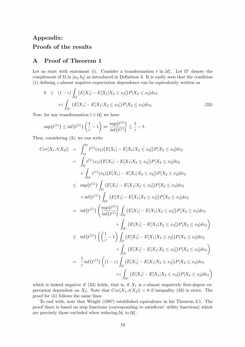
A Proof of Theorem 1

Let us start with statement (i). Consider a transformation t in Uε1 . Let Ωc denote thecomplement of Ω in [a2, b2] as introduced in Definition 3. It is easily seen that the condition(1) defining ε-almost negative expectation dependence can be equivalently written as

0 ≥ (1− ε)∫

Ω

(E[X1]− E[X1|X2 ≤ x2]

)P [X2 ≤ x2]dx2

+ε

∫Ωc

(E[X1]− E[X1|X2 ≤ x2]

)P [X2 ≤ x2]dx2. (33)

Now, for any transformation t ∈ Uε1 we have

supt(1) ≤ inft(1)(

1

ε− 1

)⇔ supt(1)

inft(1)≤ 1

ε− 1.

Then, considering (3), we can write

Cov[X1, t(X2)] =

∫ b2

a2

t(1)(x2)(E[X1]− E[X1|X2 ≤ x2]

)P [X2 ≤ x2]dx2

=

∫Ωt(1)(x2)

(E[X1]− E[X1|X2 ≤ x2]

)P [X2 ≤ x2]dx2

+

∫Ωc

t(1)(x2)(E[X1]− E[X1|X2 ≤ x2]

)P [X2 ≤ x2]dx2

≤ supt(1)∫

Ω

(E[X1]− E[X1|X2 ≤ x2]

)P [X2 ≤ x2]dx2

+ inft(1)∫

Ωc

(E[X1]− E[X1|X2 ≤ x2]

)P [X2 ≤ x2]dx2

= inft(1)

(supt(1)inft(1)

∫Ω

(E[X1]− E[X1|X2 ≤ x2]

)P [X2 ≤ x2]dx2

+

∫Ωc

(E[X1]− E[X1|X2 ≤ x2]

)P [X2 ≤ x2]dx2

)≤ inft(1)

((1

ε− 1

)∫Ω

(E[X1]− E[X1|X2 ≤ x2]

)P [X2 ≤ x2]dx2

+

∫Ωc

(E[X1]− E[X1|X2 ≤ x2]

)P [X2 ≤ x2]dx2

)=

1

εinft(1)

((1− ε)

∫Ω

(E[X1]− E[X1|X2 ≤ x2]

)P [X2 ≤ x2]dx2

+ε

∫Ωc

(E[X1]− E[X1|X2 ≤ x2]

)P [X2 ≤ x2]dx2

)which is indeed negative if (33) holds, that is, if X1 is ε-almost negatively first-degree ex-pectation dependent on X2. Note that Cov[X1, t(X2)] < 0 if inequality (33) is strict. Theproof for (ii) follows the same lines.

To end with, note that Wright (1987) established equivalence in his Theorem 3.1. Theproof there is based on step functions (corresponding to satisficers’ utility functions) whichare precisely those excluded when reducing U1 to Uε1 .

19

B Proof of Theorem 2

Let us start with the statement (i). Consider a transformation t in Uθ2,a. It is easily seenthat the condition (11) defining θ-almost negatively second-degree expectation dependencecan be equivalently written as

0 ≥ (1− θ)∫

ΩED2 (X1|x2) dx2 + θ

∫Ωc

ED2 (X1|x2) dx2. (34)

Now, for any transformation t ∈ Uθ2,a we have

sup−t(2) ≤ inf−t(2)(

1

θ− 1

)⇔ sup−t(2)

inf−t(2)≤ 1

θ− 1.

Then, considering (3), we can write

Cov[X1, t(X2)] =

∫ b2

a2

t(1)(x2)ED1(X1|x2)P [X2 ≤ x2]dx2

= t(1)(b2)ED2 (X1| b2) +

∫ b2

a2

(−t(2)(x2)

)ED2 (X1|x2) dx2. (35)

If ED2 (X1| b2) ≤ 0, then the first term is negative since t(1)(b2) ≥ 0. The second term canbe rewritten as∫ b2

a2

(−t(2)(x2)

)ED2 (X1|x2) dx2

=

∫Φ

(−t(2)(x2)

)ED2 (X1|x2) dx2 +

∫Φc

(−t(2)(x2)

)ED2 (X1|x2) dx2

≤ sup−t(2)∫

ΦED2 (X1|x2) dx2 + inf−t(2)

∫Φc

ED2 (X1|x2) dx2

= inf−t(2)

(sup−t(2)inf−t(2)

∫ΦED2 (X1|x2) dx2 +

∫Φc

ED2 (X1|x2) dx2

)

≤ inf−t(2)((

1

θ− 1

)∫ΦED2 (X1|x2) dx2 +

∫Φc

ED2 (X1|x2) dx2

)=

1

θinf−t(2)

((1− θ)

∫ΦED2 (X1|x2) dx2 + θ

∫Φc

ED2 (X1|x2) dx2

)which is indeed negative if (11) holds. Thus, if X1 is θ-almost negatively second-degreeexpectation dependent on X2, then Cov[X1, t(X2)] ≤ 0. Note that Cov[X1, t(X2)] < 0 ifinequality (11) is strict. The proof for (ii) follows the same lines.

C Proof of Theorem 3

Considering a transformation t ∈ U2,`, we can rewrite (3) as

Cov[X1, t(X2)] =

∫ b2

a2

t(1)(x2)ED1(X1|x2)P [X2 > x2]dx2

= t(1)(a2)ED2 (X1| a2) +

∫ b2

a2

t(2)(x2)ED2 (X1|x2) dx2. (36)

Thus, Cov[X1, t(X2)] ≥ 0 for all t ∈ U2,` when X1 is positively second-degree excess depen-dent on X2 and Cov[X1, t(X2)] ≤ 0 for all t ∈ U2,` when X1 is negatively second-degreeexcess dependent on X2

20

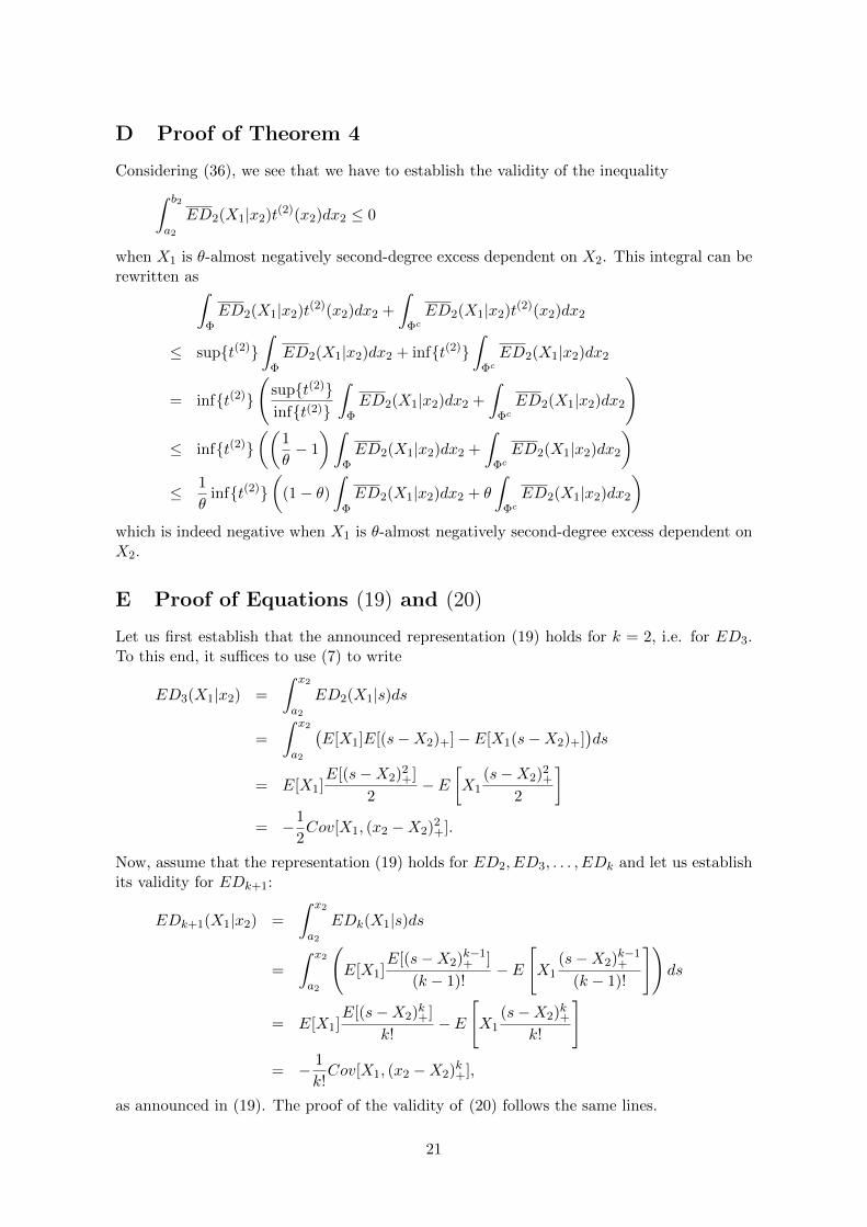
D Proof of Theorem 4

Considering (36), we see that we have to establish the validity of the inequality∫ b2

a2

ED2(X1|x2)t(2)(x2)dx2 ≤ 0

when X1 is θ-almost negatively second-degree excess dependent on X2. This integral can berewritten as∫

ΦED2(X1|x2)t(2)(x2)dx2 +

∫Φc

ED2(X1|x2)t(2)(x2)dx2

≤ supt(2)∫

ΦED2(X1|x2)dx2 + inft(2)

∫Φc

ED2(X1|x2)dx2

= inft(2)

(supt(2)inft(2)

∫ΦED2(X1|x2)dx2 +

∫Φc

ED2(X1|x2)dx2

)

≤ inft(2)((

1

θ− 1

)∫ΦED2(X1|x2)dx2 +

∫Φc

ED2(X1|x2)dx2

)≤ 1

θinft(2)

((1− θ)

∫ΦED2(X1|x2)dx2 + θ

∫Φc

ED2(X1|x2)dx2

)which is indeed negative when X1 is θ-almost negatively second-degree excess dependent onX2.

E Proof of Equations (19) and (20)

Let us first establish that the announced representation (19) holds for k = 2, i.e. for ED3.To this end, it suffices to use (7) to write

ED3(X1|x2) =

∫ x2

a2

ED2(X1|s)ds

=

∫ x2

a2

(E[X1]E[(s−X2)+]− E[X1(s−X2)+]

)ds

= E[X1]E[(s−X2)2

+]

2− E

[X1

(s−X2)2+

2

]= −1

2Cov[X1, (x2 −X2)2

+].

Now, assume that the representation (19) holds for ED2, ED3, . . . , EDk and let us establishits validity for EDk+1:

EDk+1(X1|x2) =

∫ x2

a2

EDk(X1|s)ds

=

∫ x2

a2

(E[X1]

E[(s−X2)k−1+ ]

(k − 1)!− E

[X1

(s−X2)k−1+

(k − 1)!

])ds

= E[X1]E[(s−X2)k+]

k!− E

[X1

(s−X2)k+k!

]= − 1

k!Cov[X1, (x2 −X2)k+],

as announced in (19). The proof of the validity of (20) follows the same lines.

21

F Proof of Theorem 5

Starting from (35), we get

Cov[X1, t(X2)] = t(1)(b2)ED2 (X1| b2)− t(2)(b2)ED3 (X1| b2)

+

∫ b2

a2

t(3)(x2)ED3 (X1|x2) dx2.

Continuing in this way gives

Cov[X1, t(X2)] = t(1)(b2)ED2 (X1| b2)− t(2)(b2)ED3 (X1| b2)

+ . . .+ (−1)nt(n−1)(b2)EDn (X1| b2)

+

∫ b2

a2

(−1)n+1t(n)(x2)EDn (X1|x2) dx2.

Similarly, considering (36), we can write

Cov[X1, t(X2)] = t(1)(a2)ED2 (X1| a2) + t(2)(a2)ED3 (X1| a2)

+

∫ b2

a2

t(3)(x2)ED3 (X1|x2) dx2

which finally gives

Cov[X1, t(X2)] = t(1)(a2)ED2 (X1| a2) + t(2)(a2)ED3 (X1| a2)

+ . . .+ t(n−1)(a2)EDn (X1| a2)

+

∫ b2

a2

t(n)(x2)EDn (X1|x2) dx2.

G Proof of Theorem 8

Let us consider the result stated under (i). The investor with utility function u selects λ inorder to maximize the objective function

O(λ) = E[u(λX1 + (1− λ)X2)].

The first-order condition is

d

dλO(λ) = 0⇔ E[(X1 −X2)u(1)(λX1 + (1− λ)X2)] = 0.

Denote as λ? the solution to this equation, assumed to be unique. Clearly,

λ? > 0 ⇔ d

dλO(λ)

∣∣∣∣λ=0

> 0

⇔ E[(X1 −X2)u(1)(X2)] > 0

⇔ E[X1u(1)(X2)] > E[X2u

(1)(X2)].

Define the non-decreasing transformation t by t(ξ) = −u(1)(ξ). We see that t ∈ Uεn andt ≤ 0. Then,

λ? > 0⇔ E[X1t(X2)] < E[X2t(X2)]. (37)

Let us now rewrite condition (37) as

Cov[X1, t(X2)] + E[X1]E[t(X2)] < Cov[X2, t(X2)] + E[X2]E[t(X2)]

22

⇔ Cov[X1, t(X2)] < Cov[X2, t(X2)] + (E[X2]− E[X1])E[t(X2)].

If X1 is strictly ε-almost negatively nth-degree expectation dependent on X2 then we knowfrom Theorem 6 that Cov[X1, t(X2)] < 0 since the transformation t belongs to Uεn. As t isnon-decreasing, we have Cov[X2, t(X2)] ≥ 0. Moreover, t ≤ 0 guarantees that the secondterm in the right-hand side is also non-negative when E[X1] ≥ E[X2]. This shows that theinequality (37) is indeed satisfied under the retained assumptions and ends the proof of (i).

To get the second part of (i), let us start again from the equivalence

λ? > 0⇔ E[(X1 −X2)u(1)(X2)] > 0.

Now, using the same transformation t = −u(1), we get

E[(X1 −X2)u(1)(X2)] = −E[(X1 −X2)t(X2)]

= −Cov[X1 −X2, t(X2)]−(E[X1]− E[X2]

)E[t(X2)]

which is strictly positive if X1 − X2 is strictly ε-almost negatively first-degree expectationdependent on X2 so that the first term in the right-hand side is strictly positive whereas thesecond one is non-negative.

Considering (ii), we are in a position to apply (i) twice: first to the proportion λ of initialwealth invested in asset 1 and then to the proportion 1− λ invested in asset 2. We then getthat λ? > 0 and 1− λ? > 0 which is the result announced in (ii).

23