The Relationship Between Expectation, Belief, and Anxiety in ...
Upload
khangminh22Category
view
3download
0
Musical expectation modelling fromaudio: a causal mid-level approach topredictive representation and learning
of spectro-temporal events
Amaury Hazan
A dissertation submitted to the Department of Information andCommunication Technologies at the Universitat Pompeu Fabra forthe program in Computer Science and Digital Communications in
partial fulfilment of the requirements for the degree of—
Doctor per la Universitat Pompeu Fabra
Director de la tesi:
Doctor Xavier SerraDepartament de Tecnologies de la Informació i les Comunicacions
Universitat Pompeu Fabra, Barcelona
Tesi Doctoral UPF / 2010


This research was performed at the Music Technology Group of the Uni-versitat Pompeu Fabra in Barcelona, Spain. This research was partiallyfunded by the EmCAP project FP6-IST, contract 013123.

Acknowledgements
Nicolas Wack taught me that programming is not a burden, it’s a lifestyle.Paul Brossier taught me that open source is not real-time, but when it’sopen-source and real-time it feels good. Perfecto Herrera taught me to takeit easy, to make it solid and to make it happen. Xavier Serra gave me theopportunity to be part of MTG and to start this thesis. Noemí taught menot to work on weekends, even if models of listening are fun.
The researchers I met at MTG and thanks to MTG taught me manythings too: many thanks to Bram de Jong, Gunter Geiger, Jens Grivolla,Thomas Aussenac, Julien Ricard, Alex Freginals, Xavier Forns, Xavier Ama-triain, Alex Loscos, Jordi Janer, Inês Salselas, Fabien Gouyon, Hendrik Pur-wins, Maarten Grachten, Rafael Ramirez, Anssi Klapuri, Esteban Maestre,Alfonso Pérez, Emilia Gómez, Ricard Marxer, Piotr Holonowicz, JoshuaEichen, Owen Meyers, Eduard Aylon, Cyril Laurier, Jordi Funollet and SergiJordà.
My brother taught me about personal commitment, but he works onweekends. My parents told me that a thesis should be completed after sixyears, even if models of listening are fun.
Actually, they are.
iii


Abstract
We develop in this thesis a computational model of music expectation,which may be one of the most important aspects in music listening. Manyphenomenons related to music listening such as preference, surprise or emo-tions are linked to the anticipatory behaviour of listeners. In this thesis, weconcentrate on a statistical account to music expectation, by modelling theprocesses of learning and predicting spectro-temporal regularities in a causalfashion.
The principle of statistical modelling of expectation can be applied to sev-eral music representations, from symbolic notation to audio signals. We firstshow that computational learning architectures can be used and evaluatedto account behavioral data concerning auditory perception and learning. Wethen propose a what/when representation of musical events which enablesto sequentially describe and learn the structure of acoustic units in musicalaudio signals.
The proposed representation is applied to describe and anticipate timbrefeatures and musical rhythms. We suggest ways to exploit the properties ofthe expectation model in music analysis tasks such as structural segmenta-tion. We finally explore the implications of our model for interactive musicapplications in the context of real-time transcription, concatenative synthe-sis, and visualization.
v


Resumen
Esta tesis presenta un modelo computacional de expectativa musical, quees un aspecto muy importante de como procesamos la música que oímos.Muchos fenómenos relacionados con el procesamiento de la música estánvinculados a una capacidad para anticipar la continuación de una pieza demúsica. Nos enfocaremos en un acercamiento estadístico de la expectativamusical, modelando los procesos de aprendizaje y de predicción de las regu-laridades espectro-temporales de forma causal.
El principio de modelado estadístico de la expectativa se puede aplicara varias representaciones de estructuras musicales, desde las notaciones sim-bólicas a la señales de audio. Primero demostramos que ciertos algoritmosde aprendizaje de secuencias se pueden usar y evaluar en el contexto de lapercepción y el aprendizaje de secuencias auditivas. Luego, proponemos unarepresentación, denominada qué/cuándo, para representar eventos musicalesde una forma que permite describir y aprender la estructura secuencial deunidades acústicas en señales de audio musical.
Aplicamos esta representación para describir y anticipar característicastímbricas y ritmos. Sugerimos que se pueden explotar las propiedades delmodelo de expectativa para resolver tareas de análisis como la segmentaciónestructural de piezas musicales. Finalmente, exploramos las implicacionesde nuestro modelo a la hora de definir nuevas aplicaciones en el contexto dela transcripción en tiempo real, la síntesis concatenativa y la visualización.
vii


Contents
Contents ix
List of Figures xiii
List of Tables xvii
1 Introduction 11.1 Motivation . . . . . . . . . . . . . . . . . . . . . . . . . . . . 21.2 A theory of expectation . . . . . . . . . . . . . . . . . . . . . 31.3 Prediction-driven Computational Modelling . . . . . . . . . . 4
1.3.1 Sequential Learning . . . . . . . . . . . . . . . . . . . 51.4 Expectation modelling in musical audio . . . . . . . . . . . . 5
1.4.1 Goals . . . . . . . . . . . . . . . . . . . . . . . . . . . 51.4.2 Application contexts . . . . . . . . . . . . . . . . . . . 6
1.5 Summary of the PhD work . . . . . . . . . . . . . . . . . . . 71.6 Structure of this document . . . . . . . . . . . . . . . . . . . 7
2 Context 92.1 Chapter Summary . . . . . . . . . . . . . . . . . . . . . . . . 92.2 Describing the dimensions of music . . . . . . . . . . . . . . . 9
2.2.1 What to expect - expectation of musical elements . . . 102.2.2 When to expect: expectation of time structures . . . . 15
2.3 Learning and music perception . . . . . . . . . . . . . . . . . 202.3.1 Implicit learning of auditory and musical regularities . 202.3.2 Learning non-local dependencies . . . . . . . . . . . . 232.3.3 Influence of acoustical cues . . . . . . . . . . . . . . . 242.3.4 Learning time dependencies . . . . . . . . . . . . . . . 252.3.5 Towards a statistical account of music perception . . . 25
3 Causal models of sequential learning 273.1 Chapter Summary . . . . . . . . . . . . . . . . . . . . . . . . 273.2 Models of sequential learning . . . . . . . . . . . . . . . . . . 27
3.2.1 Causal versus batch processing . . . . . . . . . . . . . 283.2.2 Markov-chain models . . . . . . . . . . . . . . . . . . . 283.2.3 N-gram modelling . . . . . . . . . . . . . . . . . . . . 283.2.4 Artificial Neural Networks . . . . . . . . . . . . . . . . 313.2.5 Applications to music modelling . . . . . . . . . . . . 38
ix

x CONTENTS
3.3 Concluding remarks . . . . . . . . . . . . . . . . . . . . . . . 39
4 Statistical learning of tone sequences 414.1 Chapter Summary . . . . . . . . . . . . . . . . . . . . . . . . 414.2 Motivation . . . . . . . . . . . . . . . . . . . . . . . . . . . . 424.3 Simulation setup . . . . . . . . . . . . . . . . . . . . . . . . . 42
4.3.1 Tone sequence encoding . . . . . . . . . . . . . . . . . 424.3.2 ANN settings . . . . . . . . . . . . . . . . . . . . . . . 434.3.3 Simulating the forced-choice task . . . . . . . . . . . . 444.3.4 Experimental loop . . . . . . . . . . . . . . . . . . . . 44
4.4 Results and discussion . . . . . . . . . . . . . . . . . . . . . . 454.4.1 Acquisition of statistical regularities . . . . . . . . . . 474.4.2 Influence of used architecture . . . . . . . . . . . . . . 474.4.3 Influence of used representation . . . . . . . . . . . . . 484.4.4 Concluding remarks . . . . . . . . . . . . . . . . . . . 48
5 Representation and Expectation in Music 515.1 Chapter summary . . . . . . . . . . . . . . . . . . . . . . . . 515.2 Automatic description of signals with attacks, beats and tim-
bre categories . . . . . . . . . . . . . . . . . . . . . . . . . . . 525.2.1 Time description: when . . . . . . . . . . . . . . . . . 525.2.2 Instrument and melody description: what . . . . . . . 525.2.3 Combining timbre and temporal Information . . . . . 53
5.3 Prediction in existing models of audio analysis . . . . . . . . 535.3.1 Audio signal prediction at the sample level . . . . . . 545.3.2 Beat-tracking as Expectation in Time . . . . . . . . . 545.3.3 Prediction-driven computational auditory scene analysis 56
5.4 Information-Theoretic Approaches . . . . . . . . . . . . . . . 585.5 Concluding remarks . . . . . . . . . . . . . . . . . . . . . . . 59
6 The What/When expectation model 616.1 Chapter summary . . . . . . . . . . . . . . . . . . . . . . . . 616.2 Motivation . . . . . . . . . . . . . . . . . . . . . . . . . . . . 626.3 Overview of the system . . . . . . . . . . . . . . . . . . . . . 636.4 Low and Mid-level Feature Extraction . . . . . . . . . . . . . 63
6.4.1 Analysis Settings . . . . . . . . . . . . . . . . . . . . . 636.4.2 Temporal detection . . . . . . . . . . . . . . . . . . . . 636.4.3 Inter Onset Intervals Characterization . . . . . . . . . 646.4.4 Timbre Description . . . . . . . . . . . . . . . . . . . . 65
6.5 Event quantization . . . . . . . . . . . . . . . . . . . . . . . . 656.5.1 Bootstrap step . . . . . . . . . . . . . . . . . . . . . . 666.5.2 Running state . . . . . . . . . . . . . . . . . . . . . . . 67
6.6 From representation to expectation . . . . . . . . . . . . . . . 686.6.1 Multi-scale N-grams . . . . . . . . . . . . . . . . . . . 686.6.2 Combining timbre and time: expectation schemes . . . 706.6.3 Scheme-dependent representation architecture . . . . . 716.6.4 Unfolding time expectation . . . . . . . . . . . . . . . 72
6.7 System evaluation . . . . . . . . . . . . . . . . . . . . . . . . 72

CONTENTS xi
6.7.1 Performance metrics . . . . . . . . . . . . . . . . . . . 736.7.2 Experiment: Loop following . . . . . . . . . . . . . . . 766.7.3 Results . . . . . . . . . . . . . . . . . . . . . . . . . . 776.7.4 Evaluation of system components . . . . . . . . . . . . 776.7.5 Expectation . . . . . . . . . . . . . . . . . . . . . . . . 796.7.6 Expected onset detection . . . . . . . . . . . . . . . . 826.7.7 Expectation entropy and structure finding . . . . . . . 83
6.8 Discussion . . . . . . . . . . . . . . . . . . . . . . . . . . . . . 846.9 Examples . . . . . . . . . . . . . . . . . . . . . . . . . . . . . 88
7 Integration in Music Processing Systems 917.1 Chapter Summary . . . . . . . . . . . . . . . . . . . . . . . . 917.2 Integration of the Representation Layer . . . . . . . . . . . . 91
7.2.1 A library for high-level audio description . . . . . . . . 917.2.2 Real-time interaction front-end . . . . . . . . . . . . . 93
7.3 Analyzing, evaluating and sonifiying . . . . . . . . . . . . . . 937.3.1 Implementation . . . . . . . . . . . . . . . . . . . . . . 957.3.2 Sonification . . . . . . . . . . . . . . . . . . . . . . . . 96
7.4 Real-Time What/When Expectation System . . . . . . . . . 967.5 Concluding remarks . . . . . . . . . . . . . . . . . . . . . . . 98
8 Conclusions 998.1 Contributions . . . . . . . . . . . . . . . . . . . . . . . . . . . 998.2 Open issues . . . . . . . . . . . . . . . . . . . . . . . . . . . . 101
8.2.1 Measuring mismatch with the environment . . . . . . 1018.2.2 Scales of music processing . . . . . . . . . . . . . . . . 1028.2.3 Towards an account of auditory learning experiments
using the what/when model . . . . . . . . . . . . . . . 1028.3 A personal concluding note . . . . . . . . . . . . . . . . . . . 103
Bibliography 105
Appendix A: Full list of publications 117Journal Articles . . . . . . . . . . . . . . . . . . . . . . . . . . . . . 117Book Chapters . . . . . . . . . . . . . . . . . . . . . . . . . . . . . 117Dissertations . . . . . . . . . . . . . . . . . . . . . . . . . . . . . . 118Conference Proceedings . . . . . . . . . . . . . . . . . . . . . . . . 118
Appendix B: Sound Examples 121


List of Figures
2.1 Three dimensional timbre space characterized by McAdams et al.(1995). Each point represent an instrument timbre label. . . . . 13
2.2 Pitch contour diagrams of three melodic schemata: axial, arch,and gap-fill, from (Snyder, 2000). . . . . . . . . . . . . . . . . . . 13
2.3 Eight of the basic structures of the Implication-Realization (I-R) model (left). First measures of All of Me (Marks & Simons1931), annotated with I/R structures (right). From (Grachtenet al., 2006). . . . . . . . . . . . . . . . . . . . . . . . . . . . . . 15
2.4 Examples of the two representations of time in music. A per-formed rhythm in continuous time (a) and a perceived rhythm indiscrete, symbolic time (b). By Desain and Honing (2003). . . . 18
2.5 Time clumping map, from (Desain and Honing, 2003) . . . . . . 182.6 Finite-state automaton used by Reber (1967) to generate letter
sequences. . . . . . . . . . . . . . . . . . . . . . . . . . . . . . . . 21
3.1 Probability distributions of single letters and bi-grams derivedfrom a corpus of English text, from (MacKay, 2003) . . . . . . . 30
3.2 Conditional probability distributions of a letter given given theprevious and the following one, from (MacKay, 2003) . . . . . . 30
3.3 A typical artificial neuron unit . . . . . . . . . . . . . . . . . . . 333.4 A typical feedforward neural network, also called multi-layer per-
ceptron. The number of hidden layers can vary. . . . . . . . . . . 333.5 A time delay neural network with two layers, processing inputs
over a context of size N . . . . . . . . . . . . . . . . . . . . . . . 353.6 A simple recurrent network, obtained by appending a context
layer to the network . . . . . . . . . . . . . . . . . . . . . . . . . 363.7 A word learning simulation presented by Elman (1990) using a
SRN predictor. The trained prediction error is plotted alongtime. The letters presented at each point in time are shown inparentheses. . . . . . . . . . . . . . . . . . . . . . . . . . . . . . . 37
4.1 Overview of the experimental setup for simulating the task de-scribed by Saffran et al. (1999) . . . . . . . . . . . . . . . . . . . 43
4.2 Forced-choice task simulation setup . . . . . . . . . . . . . . . . . 45
xiii

xiv List of Figures
4.3 Forced-choice accuracy obtained with SRN predictor for distincttone sequence encodings, compared with the subjects’ responsein (Saffran et al., 1999) . . . . . . . . . . . . . . . . . . . . . . . 46
4.4 Forced-choice accuracy obtained with FNN predictor for distincttone sequence encodings, compared with the ground truth . . . . 46
5.1 Block diagram of a prediction-driven computational auditory sceneanalysis system, from (Ellis, 1996). . . . . . . . . . . . . . . . . . 56
5.2 Diagram of the evolution of various alternative explanations froma simple example involving noise sounds, from (Ellis, 1996). Fromleft to right: a root hypothesis concerning an event occurrence ata given time gives rise to a tree of possible observations concerningfuture auditory objects. . . . . . . . . . . . . . . . . . . . . . . . 57
6.1 System diagram. Feedforward connections (left to right) create astream of symbols to be learned. Feedback connections (right toleft) enable symbolic predictions to be mapped back into absolutetime. IOI refers to Inter-Onset Interval, as explained in the nextsection. . . . . . . . . . . . . . . . . . . . . . . . . . . . . . . . . 64
6.2 Timbre clusters assigned to each event after exposure to a com-mercial drum’n bass pattern. The timbre descriptors are MFCC 68
6.3 Unclustered and clustered BRIOI histograms after exposure to acommercial drum’n bass pattern. . . . . . . . . . . . . . . . . . . 69
6.4 Graphical models of three schemes for combining what and whenprediction. . . . . . . . . . . . . . . . . . . . . . . . . . . . . . . . 70
6.5 Block diagram of the representation layer used for independentand joint expectation schemes . . . . . . . . . . . . . . . . . . . . 71
6.6 Block diagram of the representation layer used for when|whatscheme . . . . . . . . . . . . . . . . . . . . . . . . . . . . . . . . . 72
6.7 Comparison of transcription and expectation during exposure toan artificial drum pattern . . . . . . . . . . . . . . . . . . . . . . 73
6.8 Comparison of expectation statistics as a function of the numberof repetitions of a given loop . . . . . . . . . . . . . . . . . . . . 81
6.9 Comparison of expectation statistics as a function of the maxi-mum order used to provide a prediction of the next event . . . . 82
6.10 Instantaneous Entropy of timbre and BRIOI predictors for a com-mercial drum’n bass excerpt . . . . . . . . . . . . . . . . . . . . . 83
6.11 Instantaneous Entropy of the combined Timbre-IOI predictor fora piano recording . . . . . . . . . . . . . . . . . . . . . . . . . . . 84
6.12 Block diagram of the representation layer used for the when|whatin a supervised setting . . . . . . . . . . . . . . . . . . . . . . . . 87
6.13 Acoustic properties of the detected attacks, plotted along their2 first principal components. Colors and shapes indicate timbreclusters assignments. . . . . . . . . . . . . . . . . . . . . . . . . . 89
6.14 Score events versus score represented as combinations of instru-ments, extracted events and expected events for the simple discoexcerpt . . . . . . . . . . . . . . . . . . . . . . . . . . . . . . . . 89
6.15 Score of the complex funk excerpt. . . . . . . . . . . . . . . . . . 90

List of Figures xv
6.16 Comparison of score, extracted events, and expected events forthe complex funk excerpt . . . . . . . . . . . . . . . . . . . . . . 90
7.1 Screenshot of the Billaboop Drums VST plug-in. . . . . . . . . . 947.2 Screenshot of the real-time what/when expectation system, ana-
lyzing the song Highway to Hell (AC/DC, 1979) . . . . . . . . . 97


List of Tables
4.1 Parameter Set for the SRN . . . . . . . . . . . . . . . . . . . . . 44
6.1 Default parameters used for simulations . . . . . . . . . . . . . . 776.2 Timbre clustering statistics for different bootstrap settings de-
pending on the PCA desired explained variance, using groundtruth onsets . . . . . . . . . . . . . . . . . . . . . . . . . . . . . . 79
6.3 Timbre clustering statistics for different bootstrap settings de-pending on the PCA desired explained variance, using detectedonsets . . . . . . . . . . . . . . . . . . . . . . . . . . . . . . . . . 80
6.4 F-measure, computed between expected events and ground truthannotations, as a function of the expectation scheme. . . . . . . . 83
6.5 Number of percussion sound classes and number of combinationsof simultaneous classes in the two examined drum patterns . . . 88
7.1 List of configurable parameters in the Billabio application . . . . 95
xvii


CHAPTER 1Introduction
Computational modelling of music aims at providing tools that enable usto analyze, understand and interact with music. In this context, computa-tional modelling of music expectation is focusing on creating models of musiclistening which have the ability to represent musical events in a meaningfulway. This representation gives the model a predictive capability about thefuture events to be heard. Both representation and prediction processes takeplace and evolve during listening in a causal, dynamic way.
Here, we start from the audio signal and view music as a sequence ofacoustic events that are ordered through time to form musical patterns. Assuch, our definition does not focus on precise aspects of western music suchas meter or harmony. However, this representation is flexible enough toaccommodate a range of musical audio signals, from commercial music tocasual sounds and voice onomatopoeia.
The role of computational models of music expectation is to create ameaningful representation of sequences of acoustic events and to learn thestructure of those sequences through the generation of expected events. Thismakes our approach closely related to studies in music representation, per-ception, and sequential learning. Computational approaches to these phe-nomena have already been proposed in the past, however there are only afew approaches that tried to provide a bridge between real-world musicalstimuli and models of expectation.
We suggest that computational models of music expectation have the po-tential to bring new approaches to interaction with musical content, becauseof their ability to represent a stream of music and to predict it. This opensthe door to applications of real-time visualization of the musical structure,musical interaction with computers and musical gaming, to cite a few.
1

2 CHAPTER 1. INTRODUCTION
1.1 Motivation
Models of music listening have played an increasing role in the recentyears. Music listening has proved to provide many insights about cognitiveprocesses such as memory, attention or emotion. Music stimuli have beenused to derive functional brain maps of music listening using neuroimagingtechniques. This enabled to determine which cortical functions were impor-tant when listening to music, as compared to processing other stimuli suchas speech or images. Researchers have proposed computational counterpartsthat attempt to simulate some of the phenomena involved in sound and mu-sic listening. Because of the multifaceted aspects of music listening, thosemodels usually focus on a particular aspect of music perception (e.g. pitchprocessing) and can rarely process real-world music pieces. Nevertheless,those computational models have proved useful in allowing theories of musicperception to be evaluated empirically through simulations.
On a more practical side, computer scientists have proposed new com-puter tools and interfaces to help music lovers to make, discover and sharemusic. Some of these tools provide ways of extracting relevant informationfrom musical audio tracks, which is called music content analysis and hasbeen one of the major branches of the Music Information Retrieval (MIR)research (see (Downie, 2003) for an introduction). In the majority of cases,these models of music content analysis are loosely related to models of musicperception. Works in the field of content-based Music Information Retrievalaim at analyzing, indexing and managing collections of music. Music contentanalysis engines produce compact summary of musical pieces in a bottom upapproach. First, low level descriptors are computed along a musical signal.Then, these signals are averaged to form mid and high-level descriptors thatrepresent the musical piece as a signature, that is, a compact summary ofthe piece.
Recent approaches are able to summarize various aspects of a musicalpiece such as rhythm (Gouyon and Dixon, 2005), tonality (Gómez, 2006),or spectral content (Wang, 2003). The resulting signature can then be usedto perform queries among a the music collection, such as similarity, finger-printing, recommendation or playlist generation. It is not unusual to qualifythis approach as bag-of-features oriented: each item’s signature is a bag offeatures that help describing it. In this process, the time structure of themusical information is often collapsed or reduced to a few measures describ-ing the statistical properties of the signal features (e.g. average, standarddeviation).
The general work flow of content-based MIR systems does not differ dra-matically from other Information Retrieval systems that manage collectionsof images or text. In all these cases, approximations are made concerninghow the listener -the reader or observer- perceives each document. Becausefeatures are averaged through time, one strong approximation that is madein such systems is the timing of perception. The perception of our envi-ronment is nevertheless a phenomenon that evolves through time. Whenobserving a picture, subjects produce a sequence of eye saccades and thustrack the points of interest of the picture. Readers discover a text one word

1.2. A THEORY OF EXPECTATION 3
after the other and form a semantic representation which is modified andcompleted when subsequent words are read.
Similarly, listeners follow a musical piece as it unfolds through time. Dur-ing this process, each new musical event is processed as a new evidence forappreciating the piece; At each point in time the listener could ask uncon-sciously: Did I perceived something? Does the sound I just I heard gives mea feeling of repetition? Does it surprise me? Is this sound, note or chordworth remembering? What feelings does it elicitate to me? The temporaldynamics of the listening process are driven by important cognitive func-tions such as attention, representation, memory, prediction, expectation andemotion (Peretz and Zatorre, 2005). In this thesis, we emphasize predictionand expectation as the dynamic processes that govern the timeline of musiclistening. At each point in time , based on what has been heard so far, thelistener forms expectations about what is going to be heard and when it isgoing to be heard. Subsequent events are then compared to these expecta-tions. In this context, the interplay of representation, expectation generationand comparison of incoming events with former expectations forms the tem-poral dynamics of the listening process. Jones and Boltz (1989) refer to thisprocess as future-oriented attending.
Temporal dynamics are also crucial when it comes to musical performanceand practice. In a band, music practitioners can constantly follow eachother to produce a collective, synchronized, musical rendition. Non-trainedmusicians are able to follow a musical piece by tapping their feet or clappingtheir hands. If the musical piece is predictable enough, the prediction willbe correct. If a sudden change occur the predictions will be wrong during acertain time lag until the structure can be followed again. This is a dynamicbehaviour that we would like to be reflected using a computational model,and that can not be addressed with bag-of-features approaches.
Overall, our main motivation is to investigate under which conditions acomputational model a music expectation can be built, define what type ofexpectations can be generated by the model, and explore new forms of mu-sical interaction that would take advantage of such a computational model.
1.2 A theory of expectation
Researchers have attempted to define the cognitive functions elicited bymusic listening. Meyer (1956) highlighted the role of expectation in the mu-sic listening process. According to him, the listener’s expectations provide animportant tool in the process of composing a musical piece, and that musicalemotions can arise from the interplay between composition and expectations.For instance, at each point in time, the listener’s expectation can be fulfilledby the composer, making the structure easier to follow, or delayed, creating afeeling of tension. Huron (2006) refines these ideas and formulates a theorycalled ITPRA, an acronym for responses caused by Imagination, Tension,Prediction, Reaction, and Appraisal. For Huron, expectations in music andother domains arise from these five functionally distinct neurophysiologicalsystems. Each system responds to stimulations from the other systems, and

4 CHAPTER 1. INTRODUCTION
the sequential ordering of these responses creates the overall listening ex-perience. The five systems are defined by Huron as follows: “Feeling statesare first activated by imagining different outcomes (Imagination). As ananticipated event approaches, physiological arousal increases, often leadingto a feeling of increasing tension (Tension). Once the event has happened,some feelings are immediately evoked related to whether one’s predictionwere borne out (Prediction). In addition, a fast reaction response is acti-vated based on a very cursory and conservative assessment of the situation(Reaction). Finally, feeling states are evoked that represent a less hasty ap-praisal of the outcome (Appraisal).” Huron shows that the ITPRA theoryof expectation helps describing many aspects of music listening and musi-cal organization in general, and backs Meyer by suggesting that musicians“have proved the most adept at manipulating the conditions of the differentdynamic responses”. These works provide a basis for understanding that thetiming of perception influences how music is appreciated by listeners, andhelps us defining the role of expectation.
The influence of expectation in the listening process can be seen as two-fold: on the one hand, expectations can be formed in a bottom-up fashion,depending on low-level statistics of the auditory environment. This pro-cess may be regarded as largely automatic, the way it affects perception hasbeen formalized into principles such as Gestalt (Narmour, 1990) or Audi-tory Scene Analysis (Bregman, 1990). In this context, Narmour suggestedthat certain aspects of music expectation are innate to music listeners ratherthan drawn from musical experience. On the other hand, expectations canoriginate from higher level processes, and be governed by a knowledge thathas been built with the musical experience of each listener. Here, the lis-teners expectation can be influenced by learning and therefore depends onenculturation (Krumhansl, 1979; Hannon and Trehub, 2005). These higher-level expectations can in turn affect lower-level stage of music perception ina top-down fashion.
From a computational modelling perspective, these approaches to defineexpectation raise the following questions: What to expect? In other words,how do listeners represent musical events from an auditory stream such asmusic, in a way that they can form expectations on it?
1.3 Prediction-driven Computational Modelling
In his thesis, Ellis (1996) proposed a model of computational auditoryscene analysis that is driven by the prediction of incoming events. As such,this model forms a milestone for building a general model of sound percep-tion, because it addresses both issues of representation and prediction. Byusing a coarse representation of sounds - showing an emphasis on generalityrather than precision, the system can simulate experiments dealing with realworld street sounds. However, the lack of musically informed representationsmake the system impractical for representing adequately sounds in musicalmixtures.
Representation of musical signals is a complex issue that has been later
1.4. EXPECTATION MODELLING IN MUSICAL AUDIO 5
addressed by content-based MIR systems. However, many works trying tobuild predictive models in music have relied on ad hoc, symbolic repre-sentations of music. In he last two decades, many approaches have beenproposed to build symbolic models of music prediction, see (Bharucha andTodd, 1989; Todd and Loy, 1991; Mozer, 1994; Tillmann et al., 2000; Lar-tillot et al., 2001; Eck and Schmidhuber, 2002; Pearce and Wiggins, 2004).Indeed, putting aside the issue of representing the musical signal has enabledresearchers to focus on other questions that arise when investigating predic-tion and modelling it: Is prediction an innate feature or is it learned? If so,how do we learn to predict? How good are we at prediction?
1.3.1 Sequential Learning
Most of our day-to-day activities involve sequencing of actions to achievea desired goal, from sequencing words to form a sentence, to driving an au-tomobile or following directions on a road map. Lashley and Jeffress (1951)has highlighted the ubiquity of sequentiality or serial order in our behavior.Sequential learning has been investigated under different perspectives, fromneurophysiology to psychology to computational modelling. These worksaimed at defining what part of sequential prediction was innate and whatpart was acquired. Several mechanisms that influence the prediction processhave been identified, and they may be linked to conscious training. How-ever, another mechanism called implicit learning suggested the hypothesisthat subjects could learn and exploit the underlying structure of a sequenceby mere exposure to a structured sequence of events.
Some issues researchers attempt to define are the kind of structure thatcan be learned, the capacity or sequential memory, or the amount of sequen-tial context needed to perform accurate predictions. Speech, language, andmusic, due to their very sequential nature, have been considered as cases ofsequential learning. Computational modelling studies have investigated theuse of certain predictive models and compared them with behavioral data.
1.4 Expectation modelling in musical audio
We aim at developing a model of expectation that is able to form arepresentation of music from an audio stream, and generate expectationswhile “listening” to this stream. Subsequently we aim at defining how theseexpectation can be used by the system to support the listening process andto provide feedback to users of musical systems.
1.4.1 Goals
This PhD dissertation first discusses the theoretical and empirical foun-dations of music representation and expectation, and then proposes technicalapproaches to provide models and implementations that simulate these phe-nomena. The dissertation also stresses how the proposed approach can beintegrated into musical system to provide novel functionalities and applica-tions.
6 CHAPTER 1. INTRODUCTION
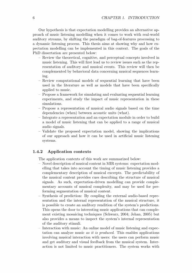
Our hypothesis is that expectation modelling provides an alternative ap-proach of music listening modelling when it comes to work with real-worldauditory streams, by shifting the paradigm of bag-of-features processing toa dynamic listening process. This thesis aims at showing why and how ex-pectation modelling can be implemented in this context. The goals of thePhD dissertation are presented below:
– Review the theoretical, cognitive, and perceptual concepts involved inmusic listening. This will first lead us to review issues such as the rep-resentation of auditory and musical events. This review will then becomplemented by behavioral data concerning musical sequences learn-ing.
– Review computational models of sequential learning that have beenused in the literature as well as models that have been specificallyapplied to music.
– Propose a framework for simulating and evaluating sequential learningexperiments, and study the impact of music representation in thesesimulations.
– Propose a representation of musical audio signals based on the timedependencies (when) between acoustic units (what).
– Integrate a representation and an expectation module in order to builda model of music listening that can be applied to a range of musicalaudio signals.
– Validate the proposed expectation model, showing the implicationsof our approach and how it can be used in artificial music listeningsystems.
1.4.2 Application contexts
The application contexts of this work are summarized below:– Novel description of musical content in MIR systems: expectation mod-
elling that takes into account the timing of music listening provides acomplementary description of musical excerpts. The predictability ofthe musical content provides cues describing the structure of musicalsignals. As such, expectation-driven modelling can provide comple-mentary accounts of musical complexity, and may be used for per-forming segmentation of musical content.
– Synthesis of prediction: By coupling the external audio-based repre-sentation and the internal representation of the musical structure, itis possible to create an auditory rendition of the system’s predictions.This opens the door to interesting music applications that can comple-ment existing mosaicing techniques (Schwarz, 2004; Jehan, 2005) butalso provides a means to inspect the system’s internal representationof the auditory stimuli.
– Interaction with music: An online model of music listening and expec-tation can analyze music as it is produced. This enables applicationsinvolving musical interaction with users: the users can perform musicand get auditory and visual feedback from the musical system. Inter-action is not limited to music practitioners. The system works with

1.5. SUMMARY OF THE PHD WORK 7
audio signals, and nonmusicians can also interact musically, like incasual games.
1.5 Summary of the PhD work
The goal of this PhD is to contribute to clarify how a causal music ex-pectation system can be applied to real-world, audio signals.
Models of music expectation have traditionally been applied to ad-hocsymbolic representation of musical events. By starting from this traditionalapproach to expectation modelling, we use a symbolic representation of mu-sical events in which case the task of an expectation model is to predict whatis coming next.
Using this setting, we define a computational framework that enables tosimulate experiments of learning of tone sequences that use the forced-choicetask paradigm (Saffran et al., 1999). Our simulations show that the abilityto reproduce behavioral data is largely influenced by the representation thatis chosen to describe musical events.
These findings lead us to define a model in which the representation ofmusical events and their expectation is linked. We propose a representationof the acoustic musical stream that takes into account both acoustic prop-erties of musical sounds (what) and the time in which they occur (when).This leads us to define a range of schemes that combine these characteristics,which form the basis of the what/when expectation model. We show thatdifferent representation models of the acoustic events -either supervised orunsupervised- can be integrated with the what/when expectation model.
The system is then evaluated using a range of musical signals contain-ing percussive sounds, monophonic melodies, or mixtures from commercialrecordings. The results suggest that fully unsupervised representation mod-els can represent and track musical signals that can be described in a mono-phonic way, whether supervised representation models are needed to tacklethe polyphonic representation of more complex sound mixtures.
Then, we show how this expectation model can be integrated in audio-processing musical systems, to enable real-time interaction, synthesis of pre-diction and visualization of both musical structure and expectation dynam-ics.
1.6 Structure of this document
The organization of this PhD dissertation is the following. In Chap-ter 2 we give an account of auditory and music perception from multiplesperspectives with the goal to illustrate how prediction has been studied andmodelled. Music perception is viewed as an active process that involves bothrepresentation and prediction of musical events, and we aim at defining howthese aspects can be combined in a simplified listening model. The musicalinformation that can be extracted when attending a musical stream, such astimbre, melody or rhythm, is presented. In our review, we use contributionsfrom (Purwins et al., 2008). Then, we report several experiments that inves-

8 CHAPTER 1. INTRODUCTION
tigate how learning of musical sequences takes place. Those works providemethods for assessing how well a set of musical stimuli can be learned bysubjects and investigate which musical structure can be learned and whatmusical factors influence learning.
In Chapter 3 we introduce computational methods of sequential learningand present past approaches to music prediction using symbolic representa-tions.
In Chapter 4, we develop a learning simulation framework in which well-known prediction methods are used to simulate a behavioral experiment fo-cusing on statistical learning of tone sequences, and stress that the choice ofthe musical representation influences learning and prediction. This chapterreports the findings published by Hazan et al. (2008). The issue of com-putational representation of musical events is developed in Chapter 5, withan emphasis on description of musical audio signals and prediction-drivenapproaches to audio analysis.
In Chapter 6, we integrate the representation and prediction layers. Weintroduce our representation and expectation models, which are aimed atgenerating expectations while analyzing audio signals by maintaining an in-ternal symbolic representation of the musical stream in terms of time andacoustic properties of musical events. We provide a set of metrics for char-acterizing the predictive behavior of the system, evaluate our model usingdifferent sets of musical excerpts, and discuss the results obtained. Thischapter uses and extends the models and findings presented by Hazan et al.(2009).
In Chapter 7 we show how the what/when expectation model can beintegrated into musical systems for providing analysis of musical signals orfor real-time applications that involve interaction and visualization.
Finally, in Chapter 8 we present the general conclusions of this disserta-tion and suggest future work directions.

CHAPTER 2Context of Research
2.1 Chapter Summary
We introduce in this chapter a number of musical dimensions that maybe considered when focusing on expectation of musical sequences. We willpresent these dimensions according to two perspectives: accounts of musicperception that are rooted in western music, and more general accounts ofauditory perception and psychoacoustics. When considering music expecta-tion, we first need to define which musical events or auditory objects can beconsidered, as well as the temporal structures that organize those objectsin musical sequences. On top of addressing the issue of music representa-tion, we aim at modelling expectation through learning of musical sequences.Therefore, in a second part, we will propose a review of auditory and musicsequence learning experiments, show the methodology employed to charac-terize how learning takes place, and show which factors influence the processof learning musical sequences.
2.2 Describing the dimensions of music: Timbre,Melody and Rhythm
Which musical dimensions should we take into account when consideringmusic expectation? Because music perception is a complex phenomenon,which can be described at various scales, this question is difficult to answer.In our approach, we aim at describing music as a sequence of auditory eventswhich are organized through time. In this simplified view, auditory eventscan consist of notes, sounds, or attacks. We will first review approachesto describe these auditory events sequences, and will then review how todescribe the temporal structures that organize these events.
9

10 CHAPTER 2. CONTEXT
2.2.1 What to expect - expectation of musical elements
When listeners listen to a musical passage, they direct their attentionand process the successive acoustic cues in a way that makes them able toidentify musical events such as notes, chords, voices, percussive strokes, etc.
In other words, listeners extract auditory objects from the stream theypay attention to, some with a better precision than others. For instance,when listening to a string section, it can be difficult or even impossible fora expert to identify how many instruments are playing together, and atwhich time is located each instrument attack. Conversely, some auditoryobjects such as a hand clap may be easier to identify and locate in time bynon-musicians.
Auditory objects
The question of how we process sound to organize it into meaningfulperceptual objects has been at the center of Bregman’s investigations. Rep-resenting sound objects in the auditory environment is mandatory in one’severyday life, for instance to locate incoming cars while crossing the streetin a noisy environment. However, those auditory objects do not necessarilyrefer to concrete sound sources, rather the refer to the mental representa-tions we create from our acoustic environment. The task of creating andmaintaining those auditory objects is called Auditory Scene Analysis (ASA,(Bregman, 1990)). Three ASA key processes are segmentation, integration,and segregation. Probably the best-known example of segregation is thecocktail party problem, in which individuals are able to segregate one par-ticular voice among many other voices and sounds. Integration of soundstakes place when different sounds are associated together to form a soundunit. This happens, for instance, when individual notes are grouped togetherand identified as a chord, or when a succession of chords is perceived as amusical color. When listening to the everyday sound environment or a musi-cal piece, the listener often hears a mixture of acoustic components and hasto identify from this mixture a representation that makes sense by isolatingindependent streams. Several factors influence how streams are segregatedfrom mixtures of sounds, an important aspects being the temporal orderingof events in the mixture.
Top-down and bottom-up processing
Top-down and bottom-up processing form two pathways involved in mu-sic perception, and have been considered in computational models. First,bottom-up processing starts from the input waveform, and successively com-bines the low level information to create more abstract cues that can be usedas input for higher-level auditory objects. Bottom-up processing is also re-ferred to as data-driven processing. Bottom-up processing is common prac-tice in Music Information Retrieval systems, where low-level descriptors areextracted from the signal (see (Peeters, 2004) for a review of such descrip-tors). These low-level descriptors are then combined to obtain higher-levelinformation, such as sound category, genre, or key. For instance, sounds

2.2. DESCRIBING THE DIMENSIONS OF MUSIC 11
with high transients and short sustain will be associated more likely to per-cussion or speech plosives than to bowed strings. Such account of musicperception through the bottom-up representation of auditory objects hasbeen developed (Schaeffer, 1966; Bregman, 1990; Roads, 2004).
Conversely, top-down processing starts from an internal representation ofthe environment and prior knowledge regarding the auditory objects, theirregularities and co-occurrences. The information flows down, by successivelycomparing a higher level representation with lower level sensory input, andadapting the higher level model to reflect the sensory input. Top-downprocessing governs several aspects of auditory perception such as auditoryrestoration, where listeners can still identify recordings of spoken wordswhere syllables have been deleted or replaced with noise bursts (Warrenand Warren, 1970), plays an important role in resolving the cocktail partyproblem (Bregman, 1990), and enable listeners to identify a specific audi-tory stream for a complex sound mixture. Top-down processing also helpsunderstanding the context effect : in a listening experiment using speech,Ladefoged (1989) has shown that listeners identify the same auditory stimu-lus at the end of a sentence as two different words depending of the beginningof the sentence.
Overall, it should be noted that bottom-up and top-down processesshould be viewed as complementary cognitive processes (Bregman, 1990).The model we will introduce in Chapter 6 provides an approach to integrat-ing both top-down and bottom-up processes, by limiting our definition ofmusical sequences to a set of acoustic units that are governed by tempo-ral patterns. Acoustic properties of sound attacks and timing informationare integrated to form a set of timbre and temporal symbols in bottom-upfashion. Conversely, musical structures can be learned and expectations canbe generated in a symbolic fashion and mapped backed into the auditorydomain in a top-down fashion. Following, we introduce the main musicaldimensions, that is, timbre, melody and rhythm, we will refer to in thisdissertation.
Timbre Perception
One of the characteristics that help distinguish between different strokes,notes or voices is timbre. The definition of timbre is still subject of contro-versy for the lack of agreement in the literature to the point that it has beenqualified as "the psychoacoustician’s multidimensional wastebasket categoryfor everything that cannot be qualified as pitch or loudness" (McAdams andBregman, 1979). Timbre is first a subjective sensation that depends on avariety of acoustic properties? According to Grey (1977),“a major aim ofresearch in timbre perception is the development of a theory for the salientdimensions or features of classes of sounds.” There is some consensus thatthe envelope of sounds as well as their spectral content affect the timbre ofa sound.

12 CHAPTER 2. CONTEXT
Among the physical quantities than may influence timbre, Schouten (1968)lists the following:
1. The range between tonal and noiselike character.
2. The spectral envelope.
3. The time envelope in terms of rise, duration, and decay.
4. The changes both of spectral envelope (formant-glide) and fundamen-tal frequency (micro-intonation).
5. The prefix, an onset of a sound quite dissimilar to the ensuing lastingvibration
Further works have attempted to characterize the perceptual dimensionsof timbre by performing listening experiments. Grey (1977) proposed acharacterization of timbre in three dimensions. In this study, subject arepresented with sounds from different instruments but whose fundamentalfrequency remains constant. The listeners rated the similarity betweenthis sounds and the results were analyzed using Multi-Dimensional Scal-ing (MDS) and related them to properties of the signal. This study hasthen been followed by (Wessel, 1979; Krumhansl, 1989; McAdams et al.,1995), in which the sound used and the experimental setup have been re-fined. Krumhansl (1989) uses three perceptual dimensions, namely attackquality, spectral flux, and brightness. In (McAdams et al., 1995), the au-thors proposed a perceptual characterization of timbre in three dimensionsalong with a computational definition of physical quantities (i.e. spectralcentroid, rise time, spectral flux) that match these perceptual dimensions.The three-dimensional space obtained is this study is shown in Figure 2.1.
Melody Perception
From a cognitive perspective, melody perception concerns primarily per-ceptual grouping. This grouping depends on relations of proximity, similar-ity, and continuity between perceived events. As a consequence, what we areable to perceive as a melody is determined by the nature and limitations ofperception and memory. Melody perception presumes various types of group-ing. One type of grouping divides simultaneous or intertwined sequences ofpitches into streams. The division into streams is such that streams are in-ternally coherent in terms of pitch range and the rate of events. A secondtype of grouping concerns the temporal structure of pitch sequences. A sub-sequence of pitches may form a melodic grouping (Snyder, 2000), if precedingand succeeding pitches are remote in terms of pitch register, or time, or if thesubsequence of pitches is repeated elsewhere. Such groupings in time mayoccur at several time scales. At a relatively short time scale the groupingscorrespond to instances of the music theoretic concepts of motifs, or figures.At a slightly longer time scale, they may correspond to phrases. Accordingto Snyder (2000), the phrase, which is typically four or eight bars long, isthe largest unit of melodic grouping we are capable of directly perceiving,due to the limits of short term memory. Rather than being fully arbitrary,(parts of) melodies are often instantiations of melodic schemata, frequently

2.2. DESCRIBING THE DIMENSIONS OF MUSIC 13
Figure 2.1: Three dimensional timbre space characterized by McAdams et al.(1995). Each point represent an instrument timbre label.
Figure 2.2: Pitch contour diagrams of three melodic schemata: axial, arch,and gap-fill, from (Snyder, 2000).
recurring patterns of pitch contours. The most common melodic schemataare axial forms, arch forms, and gap-fill forms (Meyer, 1956). Axial formsfluctuate around a central pitch, the ‘axis’; Arch forms move away from andback to a particular pitch; And gap-fill forms start with a large pitch inter-val (the ‘gap’) and continue with a series of smaller intervals in the otherregistral direction, to fill the gap (Snyder, 2000). The pitch contours of theseschemata are illustrated in Figure 2.2.
The Implication-Realization model
The most well-known model for melodic expectancy is the Implication-Realization (I-R) model (Narmour, 1990, 1992) The (I-R) model is a theoryof perception and cognition of melodies. The theory states that a melodic

14 CHAPTER 2. CONTEXT
musical line continuously causes listeners to generate expectations of howthe melody should continue. The nature of these expectations in an individ-ual are motivated by two types of sources: innate and learned. Accordingto Narmour, on the one hand we are all born with innate information whichsuggests to us how a particular melody should continue. On the other hand,learned factors are due to exposure to music throughout our lives and famil-iarity with musical styles and particular melodies. According to Narmour,any two consecutively perceived notes constitute a melodic interval, and ifthis interval is not conceived as complete, it is an implicative interval, i.e. aninterval that implies a subsequent interval with certain characteristics. Thatis to say, some notes are more likely than others to follow the implicativeinterval. Two main principles recognized by Narmour concern registral di-rection and intervallic difference. The principle of registral direction (PRD)states that small intervals imply an interval in the same registral direction (asmall upward interval implies another upward interval and analogously fordownward intervals), and large intervals imply a change in registral direc-tion (a large upward interval implies a downward interval and analogouslyfor downward intervals). The principle of intervallic difference (PID) statesthat a small (five semitones or less) interval implies a similarly-sized interval(plus or minus 2 semitones), and a large interval (seven semitones or more)implies a smaller interval.
Based on these two principles, melodic patterns or groups can be identi-fied that either satisfy or violate the implication as predicted by the princi-ples. Such patterns are called structures and are labeled to denote charac-teristics in terms of registral direction and intervallic difference.
For example, the P structure (“Process”) is a small interval followed byanother small interval (of similar size), thus satisfying both the PRD and thePID. Similarly the IP (“Intervallic Process”) structure satisfies the PID, butviolates the PRD. Some structures are said to be retrospective counterpartsof other structures. They are identified as their counterpart, but only afterthe complete structure is exposed. In general the retrospective variant ofa structure has the same registral form and intervallic proportions, but theintervals are smaller or larger. For example, an initial large interval does notgive rise to a P structure (rather to an R, IR, or VR, see figure 1, top), butif another large interval in the same registral direction follows, the patternis a pair of similarly sized intervals in the same registral direction, and thusit is identified as a retrospective P structure, denoted as (P).
Figure 2.3 (left) shows eight prototypical Narmour structures. A note ina melody often belongs to more than one structure. Thus, a description of amelody as a sequence of Narmour structures consists of a list of overlappingstructures. The melody can be parsed in order to automatically generate animplication/realization analysis. Figure 2.3 (left) shows the analysis for amelody fragment. As pointed out by Grachten et al. (2006), The I-R analysiscan be regarded as a moderately abstract representation of the score, thatconveys information about the rough pitch interval contour and, through theboundary locations of the I-R structures, it includes metrical and durationalinformation of the melody as well. It is worth noting here that the I-Rmodel rely on perception principles (proximity, similarity, closure) that are

2.2. DESCRIBING THE DIMENSIONS OF MUSIC 15
G � � � � � � � � � � � �G � � � � � � � � � � � �P D ID IP
VP R IR VR44
3
P ID P P
All Of Me
Figure 2.3: Eight of the basic structures of the Implication-Realization (I-R)model (left). First measures of All of Me (Marks & Simons 1931), annotatedwith I/R structures (right). From (Grachten et al., 2006).
not specific to melody. In this context the I-R model might be adapted toprocess sequences of auditory objects other that pitches (e.g. non-pitchedpercussive events).
2.2.2 When to expect: expectation of time structures
In parallel to forming expectations about what is going to be heard, thelistener also anticipates when the events will be heard. The interaction ofwhat and when expectation form the main basis of predictive listening inmusic. A representation of events in time has to be used to anticipate thetiming of future events. Different representations of time that may be usefulto form such expectations. We will present in this section some key conceptsto understand these representations.
Firstly, periodic auditory cues such as clock ticks are easy to predict,because the period of the cue can be processed by listeners. This is not thecase for events in which the period between cues is either too short (successiveevents will be perceived as a whole or as independent streams) or too long,in which case the perception of periodicity vanishes. Demany et al. (1977)sustains the existence of a preferred tempo spectrum ranging from 60 to 120beats per minute anchored approximately at 100 beats per minute (we referto London (2002), who provides a detailed review of cognitive constraints onbeat perception). When a musical excerpt is attended, listeners are able tofollow the most salient periodic pulse and tap in time with the music. Thenotion of tactus is associated to this most salient pulse.
From Periodicity to Rhythm
Meter represents a finer-grained description of the temporal structurewhich enables to describe musical events in a hierarchical way. As noted byTillmann (2008), "temporal regularities include the organization of event-onset-intervals through time leading to a sensation of meter - a sensationof a regular succession of strong and weak beats superimposed over anisochronous pulse. Temporal regularities also include the temporal patternsof onset intervals creating rhythms that are perceived against the metricalbackground". As Huron (2006) points out, meter may also be seen froma prediction-driven perspective. Huron points out that “Meter provides arecurring temporal template for coding and predicting event onsets.”. If asequence of inter-onset intervals has a regular period, “the temporal expec-

16 CHAPTER 2. CONTEXT
tations might be represented using mental oscillators of various frequenciesand phases”. Then, by considering where the onsets are located along thesequence period, the listener may be able to locate the onset moments thatare more likely than others. This gives rise to a hierarchy of temporal events“which can be expressed in terms of their metric position within a recur-ring temporal template”. To this extent, meters can be viewed as predictiveschemas that enable expectation of temporal events. The time expectationmodel we propose in Chapter 6 aims at learning the time regularities be-tween acoustic objects. We will suggest that the prediction statistics of suchregularities can give rise to a rough, implicit representation of meter.
On a more precise scale, a musical sequence can be described in termsof rhythm. Rhythm is a musical concept with a particularly wide range ofmeanings, and as such it is essential to delimit the scope of what we will betalking about when discussing rhythm. An all-encompassing description ofrhythm would be that it is about the perception of the temporal organiza-tion of sound. As far as we consider musical sound, rhythm in this senseis tightly connected with the concept of meter. Several studies have evenquestioned the separation between the processes of meter and rhythm per-ception altogether (Hasty, 1997; Rothstein, 1981; Drake, 1998; Lerdahl andJackendoff, 1983).
Although rhythm is ambiguous and could, as in the bottom-line definitiongiven above, also include meter, a common use of the words rhythm andmeter is expressed in a paraphrase of London (2006): “Meter is how youcount time, and rhythm is what you count–or what you play while you arecounting”. When we hear a sequence of events that can be located in time,periodicities in the timing of these events will cause in us the awareness of abeat, or pulse. By this, we mean a fixed and repeating time interval with aparticular offset in time, that can be thought of as a temporal grid, forminga context in which the perceived events take place. The perception of eventsoften makes some beats feel stronger, or more accented, than others, givingrise to a hierarchical grid of beats.
As a context for the perception of musical events, meter serves to catego-rize events in terms of temporal position and accent, and inter-onset intervals(IOI) of events in terms of duration. A common interpretation of rhythmis the grouping of sequences of such categorized events, where groups oftencontain one accented event and one or more unaccented events (Cooper andMeyer, 1960). This accounts for the influence of meter on the perceptionof rhythm. The perception of actual musical events on the other hand alsoaffects the perception of meter. Firstly, in actual performances phenomenalcues like the loudness and duration of events are used to accent particularmetrical positions, thereby suggesting a specific meter (Lerdahl and Jack-endoff, 1983; Palmer, 1989). In addition to this, the frequency distributionof musical events over metrical locations is mainly correlated with meter,rather than, for example, musical style or period (Palmer and Krumhansl,1990). This indicates that frequency distribution of events in a piece couldbe a perceptual clue to determining meter. Palmer and Krumhansl (1990)also show that listeners appear to have abstract knowledge of the accentstructure of different kinds of meters, which become more fine-grained as a

2.2. DESCRIBING THE DIMENSIONS OF MUSIC 17
result of musical training. They suggest that the accent structures of differ-ent meters are learned by virtue of their ubiquity in Western tonal music.
A first step towards the understanding of rhythm perception is the studyof perceived event durations. Differentiation of event durations happens inan early stage of auditory processing. Several factors are known to affect theperceived durations, leading to a difference between the physical durationand the perceived duration of an event. These include the phenomenon ofauditory streaming, intensity/pitch difference between evenly spaced notes,and metric context. Likewise, perceived inter-onset intervals are influencedby event durations, and the different durations of successive events in theirturn can affect the intensity and/or loudness perception of these (Terhardt,1998).
Listening to two successive acoustic events gives rise to other cognitiveprocesses than listening to each event separately. The judgment of successiveevents can be divided into two steps. The first step follows a modified versionof Weber’s law, in which the just-noticeable difference between two successivedurations is proportional to their absolute length plus a constant of minimaldiscrimination (Allan, 1979). The second step consists in comparing the twodurations. If they are similar, the second duration is related to the firstone. If the two durations are considered very different they will both berelated to previously established perceptual categories of durations (Clarke,1989). Following, we will present several experiments that investigate howthe quantization of rhythm takes place in listeners.
Rhythm quantization
Desain and Honing (2003) present two experiments to analyze the for-mation of perceived discrete rhythmic categories and their boundaries. Thenotion of rhythmic categories is interesting because those discrete categoriesrefer to rhythms defined by continuous durations. In the first experimentthey study the phenomenon of rhythm categorization, which consists in themapping from the performance space –the set of possible performed IOIdurations– to a symbolic space of rhythm representation –the set of dura-tion categories, or nominal durations. An example comparing these tworepresentations is shown in Figure 2.4.
Such a mapping expresses how much the IOI’s of a performed rhythmicpattern can deviate from the nominal IOI durations that define the pattern,before it is being perceived as a different rhythmic pattern. The deviationfrom the nominal IOI durations is called expressive timing. Listeners tendto simplify durational relations assigned to an expressively timed patternof onsets. Here, high consistency in the listener’s judgment is predominantif the durational ratios are simple. Figure 2.5 shows the time clumpingmap that can be extracted from this experiment, by associating perceivedrhythmic categories to triplets of performed inter-onset intervals.
In the second experiment, Desain and Honing study how the metrical con-text affects the formation of rhythmic categories. As a context, an acousticpattern is provided by tapping a triple, duple, and simply a bar structure.Then the stimulus is played. Given triple and duple meter contexts, the

18 CHAPTER 2. CONTEXT
Figure 2.4: Examples of the two representations of time in music. A per-formed rhythm in continuous time (a) and a perceived rhythm in discrete,symbolic time (b). By Desain and Honing (2003).
Figure 2.5: Time clumping map obtained after a listening experiment. Thethree triangle axes indicate the performance time as inter-onset intervals be-tween successive strokes. The colored region refer to the symbolic categoriesthat were chosen by the participants. Darker colors indicate a greater agree-ment between participants. Grey lines mark boundaries between rhythmcategories. White regions indicate regions of low agreement among partici-pants regarding the perceived rhythmic category. From (Desain and Honing,2003).
stimulus is identified as having the meter of the context stimulus. If onlybars are sonified, the stimulus is as well identified as duple meter in themajority of the cases.
As noted by Hannon and Trehub (2005), when listeners have categorizeddurations, they will continue to interpret new temporal patterns in terms ofthe formed categories, even in the presence of perceptible temporal changes

2.2. DESCRIBING THE DIMENSIONS OF MUSIC 19
(Clarke, 1987; Large, 2000).We retain from this overview that both performance and perceptual rep-
resentations of time may be considered when representing timing in music.This gives us a basis to consider the representation of time from two view-points: an absolute, precise and sensor driven representation (referred to as“performance” time by Desain and Honing (2003)) and a compact, discreterepresentation of time symbols. To this extent, we suggest a model thatmay be able to manage both representation should implement mechanismsto translate the time information between these representations.
Rhythm along several acoustic dimensions Going back to figure 2.4we observe that the rhythm stimulus that is considered is made of a singleclass of stroke. For the sake of simplicity, the only absolute information thatis considered is the duration between successive strokes. We could argue thatmany popular rhythms (think about a rock drum performance) are using amore extended set of strokes (e.g. tom, cymbal, etc ...). The individual char-acteristic of each stroke (accent, instrument) provides additional informationthat may be used to encode the musical rhythm. For instance, being ableto segregate the tom strokes form the cymbal strokes enables to track thestroke dependencies between events of the same acoustic category. This isan example of how top-down processing can influence lower-level representa-tion layers. As we will see in Section 2.3.3, the acoustic similarities betweenstrokes and notes can affect the way a musical sequence is learned. This willalso form a basis for the computational model we propose in Chapter 6.

20 CHAPTER 2. CONTEXT
2.3 Learning and music perception
So far we have reviewed aspects of music perception that enable to definea musical stream under various modalities (pitch, timbre, time and rhythm).In the context of this dissertation, we are interested in investigating the roleof expectation and its interplay with the representation with musical events.As we stressed in the introduction, this interplay can take place at severallevels of abstraction. First, low-level expectation processes take place in aunconscious, automatic, hardwired fashion, and are reflected in AuditoryScene Analysis and Gestalt approaches. Then, higher-level expectation pro-cesses may be the result of a knowledge of the musical environment, thatis acquired through experience. Several works have shown that an implicitknowledge about tonal structures can be acquired by mere exposure to tonalmusic and will be presented below. More generally, this section introducesworks that aim to answer how we learn musical sequences and what musicalaspects influence learning.
Apart from the hypothesis raised and results obtained, we will intro-duce the methodology used to understand the experimental setup employedas basis for the simulation framework we will introduce in Chapter 4. Onemajor difficulty here is that the music we listen to on a daily basis, the "real-world" music, is usually too complex to be used in behavioral experimentswhere few parameters are to be varied, while many other need to be fixed,to obtain significant conclusions. However, we will show that these stud-ies converge towards a common learning principle which takes place alongseveral dimensions of music.
2.3.1 Implicit learning of auditory and musical regularities
In the 1960s, Reber pioneered the use of artificial grammars to inves-tigate how these grammars could be learned by human subjects. Reber’swork focused on the mechanism of implicit learning which suggests that thecommon structure of stimuli can be learned by means of mere exposure tothose stimuli. To demonstrate this, the author generated sequences of let-ters using a finite state automaton (FSA) as shown is Figure 2.6. Sequencesgenerated using this FSA share a common underlying structure, even if theydiffer in size. Participants were then presented novel sequences and asked ifthese sequences were grammatical or not. Reber measured how well thesesequences could be memorized by subjects and showed that the results sig-nificantly outperformed those obtained with randomly generated sequences(Reber, 1967).
This phenomenon of implicit learning takes place independently of themodality of the visual stimuli (colors, letters, shapes). Subsequent workshave translated these findings into the auditory domain. In this case, thesequences of letters are replaced by sequences of sounds. Tones are used byAltmann et al. (1995); Saffran et al. (1999); Loui et al. (2006).
In (Bigand et al., 1998a), the sequences are made of sounds with distincttimbres, whereas they consist of speech phonemes in (Saffran et al., 1996).Those studies have also employed various methods to generate exposure se-

2.3. LEARNING AND MUSIC PERCEPTION 21
Figure 2.6: Finite-state automaton used by Reber (1967) to generate lettersequences.
quences. The underlying structure to be learned from exposure sequencescan be derived from transition probabilities (Saffran et al., 1996, 1999; Till-mann and McAdams, 2004), finite-state automata (Loui et al., 2006), orgrammars (Bigand et al., 1998b). Among those works, there is a commonagreement that the structure of auditory sequences can be learned by mereexposure.
Therefore, investigating music perception from an implicit learning per-spective may provide a complementary account to the music perception the-ories presented in Section 2.2, that do not focus explicitly on the learningprocess. We will provide in Chapter 4 a modelling study that shows howprediction and implicit learning are related. To achieve this, we need to un-derstand the methodology employed to highlight implicit learning in musicalsequences.
Learning statistical triplets in speech and tone sequences
Saffran et al. (1996, 1999) focused on assessing whether humans canlearn regularities related to the transition probabilities regulating the ele-ments inside auditory units (called words) or the word transitions in audi-tory material. In (Saffran et al., 1996) the auditory material was made ofsynthesized speech syllables, while in (Saffran et al., 1999) the authors usedtone sequences, preserving the previous experimental setup. The authorscreated a set of artificial stimuli by setting high inside-word and low across-boundaries transition probabilities. In this work, two languages L1 and L2were created. Each one contained 6 tone triplets, called tone-words. First,a random sequence of words of the defined language was presented to thesubjects. However the tone triplets were presented in a regular order. Therewas no explicit cue indicating the boundaries among them. This means thatthe presented material appeared as a stream of tones which could be only

22 CHAPTER 2. CONTEXT
segmented using the statistical regularities of words. In the first experiment,words from L1 were non-words in L2, and vice versa. That is, there wasno word in one language that appeared, even partly, in the other language.In the second experiment, words from one language were part-words in theother language, that is, only one tone differed between each language word.After exposure, the subjects had to perform forced-choice tasks involvingexhaustive word-pairs belonging to each language. The task consisted inchoosing which word of the pair had been effectively heard in the presentedmaterial. This study pointed out that the subjects were able to categorizeabove chance the words belonging to the material they were exposed. Thismeans that the subjects are able to segment the input stream into words andto distinguish if a word presented subsequently belongs to the sequence theyhave been exposed to, and suggests that an automatic learning mechanismthat exploits the co-occurrences of tones takes place.
Non western music scales
Loui et al. (2006) investigated the emergence of statistical regularitiesbased on the presentation of non-western tonal sequences, generated usingusing the the Bohlen-Pierce scale (Mathews et al., 1984). Indeed, westernlisteners are mostly exposed to music using the western scale, so using anon-western scale to assess tone-word learning enables to discard the effectof enculturation in the learning process. In (Loui et al., 2006), the tonesequences were derived from two distinct finite state grammars, with someconstraints (they respect the Narmour principle of closure). This work in-vestigates whether the participants can acquire aspects of the structure ofthese two grammars using (a) forced-choice recognition and generalization(b) pre and post-exposure probe tone ratings, and (c) preference ratings.The authors introduced two experimental settings: in the first one a fewexposure melodies were presented, while in the second one the number ofexposure melodies (following a unique exposure grammar) was multipliedby three. As a general conclusion, the participants in experiment 1 tend torecognize better the melodies they have been exposed to while some in ex-periment 2 (the ones exposed to grammar 1) are also able to recognize newmelodies generated from the grammar they have been exposed to (i.e. gen-eralization). Furthermore, the post-exposure probe tone ratings were morecorrelated with the statistical distribution of the stimulus notes. Overall,the works presented above show that subjects are able to identify whethernovel sequences respect or violate the structure of the exposure sequences.
This suggests that implicit learning also applies in auditory sequencesunder several modalities. One question arises from this: can the severaldimensions that define a musical sequence have an influence on each otherin way that makes it easier or harder to learn this sequence?

2.3. LEARNING AND MUSIC PERCEPTION 23
Learning statistical regularities in timbre sequences and theinfluence of timbral similarity
Tillmann and McAdams (2004) investigated the relation between acous-tical similarity and statistical regularities in auditory sequences generatedusing different instruments. The authors proceeded by creating three setsof stimuli. The authors defined statistical timbre triplets by analogy withSaffran’s work. In the first set, the statistical regularities were supportedby acoustical similarities, i.e. the "timbral distance" between inner-worditems was low while it was high across word boundaries. In the second set,the acoustical similarity contradicted the statistical regularities of the stim-uli. Finally, in a third set, the timbral distance between consecutive eventswas neutral with respect to the statistical regularities. As a result, the au-thors found than subjects could learn timbre triplets from the first set witha higher accuracy than using the other sets. The worst learning accuracywas achieved using material where the acoustical cues were contradicting thestatistical regularities of the auditory sequence. This work showed that thetimbre information contained in auditory sequences influences the recogni-tion of statistical units. Acoustic cues that support the statistical structureof timbre sequences facilitate the learning process. When the timbre in-formation contradicts the same statistical structure, learning becomes moredifficult.
2.3.2 Learning non-local dependencies
So far, we have considered how learning takes places for auditory se-quences where adjacent events share a common structure. From this view-point, tones, sounds or phonemes are organized so that the transitions be-tween successive events define this structure. However, musical sequencescan also exhibit non-adjacent dependencies. To understand these non-localdependencies, let’s consider a musical example. A melody is defined as asuccession of notes that may have a complex structure, if we try to de-fine this structure in terms of transitions between adjacent events. How-ever, this apparently complex sequence can reveal two simpler interleavedmelodies, such as a bass line and a main melody line. Therefore, we are inter-ested in knowing how implicit learning takes place in a context of non-localdependencies. Past research on sequential order has shown that implicitlearning of non-local patterns was generally difficult and that learners couldlearn patterns of temporally adjacent elements much better that they couldlearn non-temporally adjacent patterns (Cleeremans and McClelland, 1991;Cleeremans, 1993).
If we go back to the example of two interleaved melodies, the intuitionwould suggest that the bass line and main melody lines can be segregated bythe listener because of the acoustical features that are common to each line.This acoustical features could include loudness, pitch or the characteristictimbre of the instrument used. If segregation can be successfully achieved(e.g. the bass line and main melody are perfectly identified), the problem isreduced to learning the local dependencies between elements of each stream.

24 CHAPTER 2. CONTEXT
Conversely, if errors are made during segregation (e.g. two streams aresegregated, but both streams consist of interleaved notes from the bass andmelody lines), the local dependencies between elements of each stream wouldnot exhibit a clear structure. Further research has attempted to define towhat extent acoustical cues can affect the learning of non-local dependencies.
2.3.3 Influence of acoustical cues
Newport and Aslin (2004) investigate how learning of non-local depen-dencies take place for speech stimuli, and report a similar study focused ontone sequences in (Creel et al., 2004). In both cases they propose a set ofexperiments focused on learning temporally non adjacent patterns and as-sessed whether acoustical cues could influence learning. The stimuli used inthese experiments are similar to those used in (Saffran et al., 1999), but inthis case the transition probabilities are defined between non-adjacent items.Two sets of items sharing are created, each one governed by its own transi-tion probabilities, and the items of each set are then interleaved to form theexposure sequences. In the first experiment, the subjects are presented anexposure sequence where the items from both sets share the same acousticalfeatures. Hence, apart from the nonlocal dependencies that govern each set,there is nothing that can help discriminating items from one set or the other.Acoustic cues are then introduced and applied on items from each set. In thecase of tone sequences, items from a given set are rendered one octave lower(experiment 2), with a a sharply different timbre (experiment 3), or withmoderately different timbre (experiment 4). In the case of speech, sequencesof vowels (respectively consonants) are created, each item of the resultingsequence is then interleaved with unrelated consonants (respectively vowels).
The authors find similar results in both studies. They first confirm withthe experiment the inability of learning highly consistent nonlocal depen-dencies in absence of acoustical cues, whether learning of local dependenciescan be achieved successfully, as is was shown in (Cleeremans, 1993). Then,they show with the subsequent experiment that if acoustical cues are used toinduce dissimilarities between the two sets, subjects can learn the structureof each set and therefore learn the dependencies between nonadjacent items.
The works presented above highlight the interplay between statisticaldependencies - using low or high order context- and acoustical cues takingplace when learning auditory sequences. Non-local dependencies cannot belearned without the help of acoustical cues that help the listener to segregatesstreams. This suggests that a model of acoustic sequence learning maytake advantage of the events acoustic information and form streams as apreliminary process to sequence learning. We will get back to this pointwhen exploring alternative expectation models applied to audio signals inChapter 6.

2.3. LEARNING AND MUSIC PERCEPTION 25
2.3.4 Learning time dependencies
In the studies mentioned above, what matters is the ordering of auditoryevents and the acoustical cues that are used. However, they do not take intoaccount the time structures (we refer to Section 2.2.2) that govern the occur-rence of acoustic events. Compared to the amount of studies investigatingimplicit learning in auditory sequences, only a few works have validated, withbehavioral experiments, the issue of how learning of time structures takesplace. Boltz (1993) has shown that temporal dependencies can support theprocess of melody recognition. Hannon and Trehub (2005) investigate howrhythm structures are learned and the influence of cultural bias to learning.Indeed, rhythm patterns make possible to link remote events into a singlestream, enabling their co-occurrences to be learned to some extent. Theauthors use two sets of rhythms to be learned, the first set has a simplemetrical structure (temporal dependencies can be expressed with simple ra-tios such as 1/2), while the second group use complex rhythms. Using aforced-choice task setup, they asked participants to classify novel sequencesas preserving or violating the exposure sequences. The results shown thatNorth-American adults could learn to recognize the simple rhythms but wereunable to learn the complex rhythms while Bulgarian or Macedonian adults-whose musical culture makes a more frequent use of complex rhythms- couldperform both tasks. This enculturation bias was confirmed with a last ex-periment, where North American infants were shown to be able distinguishstructure-preserving complex rhythms from structure-violating sequences.This suggests that the musical environment North American infants are ex-posed to during development has overridden their initial ability to apprehendcomplex rhythms, because this ability is not useful in their environment.
2.3.5 Towards a statistical account of music perception
The works we have presented here focus on the various dimension we useto define musical sequences, i.e. timbre, pitch, and time. Independently ofthe modality used, these studies show that the common principle of implicitlearning holds, that is, that mere exposure to sequences of events enablesto learn to represent the structure of these sequences. Furthermore, the in-terplay between temporal and acoustical cues can enable to learn non-localdependencies, which would be too difficult to learn otherwise. More workhas to be done to be able to deal with the complexity of real-world mu-sic. As Tillmann (2008) states, "Experimental research on music perceptionhas to find a balance between the complexity of real musical material andstrong experimental control of the used material leading to the use of sim-ple tone contexts or melodies". However, despite the actual limitations ofthese works, we aim at integrating the general results obtained here in acomputational model of music expectation.
Therefore, we will focus on building a model that can acquire a represen-tation of musical structure through exposure, according to the principle ofstatistical learning. Our first motivation is to create a “blank” listener modelguided by representation and learning principles. In this approach, the envi-

26 CHAPTER 2. CONTEXT
ronment will induce an internal model that will serve as a basis for generatingexpectations, instead of attempting to hard-wire a specific and static musictheory in the model. The key questions that arise at the point are: what arethe computational architectures that can be used to implement statisticallearning systems and how can such architecture be evaluated. This questionswill be answered in the two forthcoming chapters, where we will first define arange of models that can perform causal learning of sequential structure, andpropose a use-case for evaluating such models based on Saffran et al. (1999).Furthermore, our review has shown that statistical learning may take placealong several musical dimensions (e.g. timbre, melody, rhythm) and showedthat learning may be facilitated when considering several dimensions insteadof focusing on one. Because we aim at processing audio excerpts, we willpropose, in Chapter 6, a set of representations of the audio stream in termsof acoustic cues and timing events, and investigate how these two dimensionscan be combined.

CHAPTER 3Causal models of
sequential learning andapplications to music
3.1 Chapter Summary
In this chapter, we introduce models of sequential learning and presentcomputational approaches that have been used to simulate this phenomenon.As such, this chapter introduces the modelling formalism that will be usedin this dissertation. We give an emphasis to causal models, that is, modelwhose predictions only depend on past observations, because causality pro-vides a natural framework for modelling sequential learning. Furthermore,to reflect the existing work on sequence learning modelling and music se-quence learning in particular, most of the approaches we present here areeither symbolic approaches or are employed to process sequences representedin a symbolic way.
3.2 Models of sequential learning
A important core of computational techniques have been developed inthe last 50 years to perform sequence analysis and prediction tasks. Thespectrum of methods ranges from periodicity analysis (such as autocorre-lation, time-frequency methods such as Fourier or wavelet transform), toartificial neural networks and probabilistic approaches. Predictive modelshave been used as forecasting application in many fields such as industry,finance or medicine (Box et al., 1976). Here, we focus on modelling learningas a dynamical process that evolves through time. This is why we make adistinction between causal and non-causal techniques, as explained below.
27
28 CHAPTER 3. CAUSAL MODELS OF SEQUENTIAL LEARNING
3.2.1 Causal versus batch processing
We aim to distinguish techniques that rely on a entire sequence to parseit from techniques that build and maintain a representation of the sequenceaccessed so far without being able to look ahead in the future. The formertechniques are referred to as batch techniques - they operate on a batch ofdata from the beginning to the end, while the latter approaches are referredto as causal approaches. Formally, a causal system, is a system whose stateat a specific instant t0 depends only on the input xt for values of t less orequal than t0.
3.2.2 Markov-chain models
In mathematics, a Markov-chain is a stochastic process which respects theMarkov property Markov (1971). This means that future states depend onlyon present states and are independent of past states. That is, the definitionof the present state fully defines the evolution of future states. Formally, AMarkov chain is a sequence of variables X1, X2, X3, ...,Xn,Xn+1 so that
Pr(Xn+1|Xn, ..., X3, X2, X1) = Pr(Xn+1|Xn) (3.1)
A variation of this is the Markov chain of order N , where N is finite.The state of this process can be written down as:
Pr(Xn+1|Xn, ..., X3, X2, X1) = Pr(Xn+1|Xn, Xn−1, ..., Xn−N ) (3.2)
Here, N acts as a memory of fixed size. Hence, a Markov chain of order N isa process in which the future state Xn+1 is fully defined by a fixed numberof past observations. This assumption is the basis of many learning modelsthat base their predictions on a past context of fixed size.
3.2.3 N-gram modelling
N-gram modelling provides a straightforward and efficient approach toprobabilistic reasoning and expectation. This approach fits well to symbolicsequence modelling approaches, where each sequence item belongs to a fixedset of possible symbols. The basic idea is to construct tables of transitionprobabilities from subsequences of N − 1 items to the next item by countingtheir occurrence in a set of training data.
We illustrate this by taking an example from MacKay (2003), focusingon modelling transition probabilities between letters (including the spacecharacter) in English sentences. Here, we consider the simple case whereN = 2, also referred to as bi-gram modelling. Let us consider the randomvariable X, which corresponds to the outcome of a letter in the Englishcorpus. The outcomes of X can be any letter of the alphabet, plus the spacecharacter. Similarly, we can define a random variable Y , which correspondsto the outcome of the following letter. Based on the training corpus, the firststep consists in counting the occurrence of each single letter. By normalizingthese counts, one can derive the marginal probability distribution of letters,

3.2. MODELS OF SEQUENTIAL LEARNING 29
denoted P (X), as shown in Figure 3.1a. In a similar way, one can count allthe sequences of two letters that occur in the training corpus, and derivethe joint probability distribution, denoted P (X,Y ). Figure 3.1b shows ina graphical way the probability distribution of such bi-grams. Here, theprobabilities are represented as white squares in a two-dimensional tableand sum to one. Based on the probabilities of occurrence of single lettersand bi-grams, we can then derive the transition probabilities between twoconsecutive letters by computing the conditional probability between a lettergiven the outcome of the previous one:
P (Y |X) =P (X,Y )
P (X)(3.3)
Similarly, it is possible to derive the conditional probability of a letter giventhe outcome of the following one.
If we return to our example, the resulting transition probabilities forthe English text corpus are shown in Figure 3.2. As an outcome of thisprocess, the transition probability tables can now be used for prediction andexpectation generation task. Indeed, when parsing a novel English sentence,it is possible, at each point in time, to obtain the condition probabilitydistribution of the next letter.
We can now define N-grams as a function of the order parameter N .When a new event xt is appended in the input sequence, a two-dimensionaltable, indexing the occurrences of all possible sequences of length n, is in-cremented by one at the position with row corresponding to the sequencext−N+1 ... xt−1 and at the column corresponding to the symbol xt. Thismeans the count table has nsymbolsN cells, where nsymbols is the numberof possible symbols. As such, this technique is expensive in terms of space,even if we can use sparse matrix implementations to reduce the size of thetransition tables. From the count table and an observation of the actual se-quence, we can derive the posterior probability for each possible symbol andproduce an expectation accordingly. The N parameter controls the amountof past events considered in the prediction and has to be adjusted carefully.Indeed, an inaccurate choice of N may affect the behavior of the learnerby biasing it to too general predictions (low N), and to over fit prediction(high N). Extensions have been proposed to combine predictions made fromdifferent context sizes.
Overall, the example we presented here gives a overview of the differ-ent processes involved in N-gram modelling. However, this example is alsomisleading , because it starts from the analysis of corpus of English text,derives knowledge from it, and then enables to perform prediction. As amatter of fact, there no need of a training corpus nor to separate learningand prediction. N-gram models can be applied in a causal way to symbolicsequences, by constantly updating their probability tables and by providingprediction based on the current tables. This way of coupling learning andprediction processes may precisely serve as basis for tackling the mechanismof implicit learning in the context of musical processing. Here, the continu-ous exposure to structured musical streams will substitute the corpus-basedtraining shown in the English letters example.

30 CHAPTER 3. CAUSAL MODELS OF SEQUENTIAL LEARNING
i ai pi
1 a 0.0575
2 b 0.0128
3 c 0.0263
4 d 0.0285
5 e 0.0913
6 f 0.0173
7 g 0.0133
8 h 0.0313
9 i 0.0599
10 j 0.0006
11 k 0.0084
12 l 0.0335
13 m 0.0235
14 n 0.0596
15 o 0.0689
16 p 0.0192
17 q 0.0008
18 r 0.0508
19 s 0.0567
20 t 0.0706
21 u 0.0334
22 v 0.0069
23 w 0.0119
24 x 0.0073
25 y 0.0164
26 z 0.0007
27 _ 0.1928
a
b
c
d
e
fg
h
ij
k
l
m
n
op
q
r
s
t
u
v
w
xy
z
_
(a)
a b c d e f g h i j k l m n o p q r s t u v w x y z _ y
abcdefghijklmnopqrstuvwxyz_
x
(b)
Figure 3.1: (a) Probability distribution of single letter P (X) and (b) bi-grams probabilities P (X,Y ) derived from counting their occurrences in acorpus of English text. Adapted from MacKay (2003).
abcdefghijklmnopqrstuvwxyz_ y
abcdefghijklmnopqrstuvwxyz_
x
abcdefghijklmnopqrstuvwxyz_ y
abcdefghijklmnopqrstuvwxyz_
x
(a) P (y |x) (b) P (x | y)
Figure 3.2: (a) Conditional probabilities of letter given the previous oneP (Y |X) and (b) conditional probability of a letter given the next oneP (X|Y ) (b). These transition probabilities are derived from the single let-ter and bi-gram probabilities shown in Figure 3.1. Adapted from MacKay(2003).

3.2. MODELS OF SEQUENTIAL LEARNING 31
Variable order markov-chain approaches
Extensions to markov chain models of fixed order have been proposed inthe context of compression algorithms research. First, Incremental Parsing(IP, Ghezzi and Mandrioli (1979)), an online method based on compressiontheory. Another approach is based on Prediction Suffix Trees (PST, Allauzenet al. (1999)). Whereas a a markov chain of order M can be represented asa tree where all branches are of size M, in PST the size of the tree branchescan be lower or equal to the maximum model order, which reduces thememory requirements of the model. Finally, an extension of N-grams, calledPredictive Partial Match (PPM, Cleary and Witten (1984); Moffat (1990)),enables to combine transition tables of different context sizes. PPM will bepresented in more details in Chapter 6.
3.2.4 Artificial Neural Networks
Artificial neural networks (ANN) form a branch of mathematical modelsthat has been motivated by the structure and functional organization of bi-ological systems. They consist of groups of interconnected artificial neuronsthat process information in a distributed way. Each artificial neuron is asimple unit that has its own activation state and is connected to other unitsvia synaptic weights. The state of a given unit is determined dependingof activations and weights of incoming units and the activation function ofthis unit. Synaptic connection can be either directed or undirected. For thesake of simplicity, we start introducing the typical case of feedforward neu-ral networks, and will derive from this architectures that are able to modelsequences of events. There are, however, more complex alternatives to thisapproach, which we will present in section 3.2.4. First, we show in Figure 3.4how an artificial neuron is represented.
The activation function of each unit is arbitrary and does not need tobe linear, which make ANN capable of non-linear transformation of data.Sensory inputs can be fed to the network and mapped to a useful repre-sentation which depends of the task considered. Formally, the incomingweighted inputs to a artificial unit j are first summed:
netj =∑i6=j
wijxi (3.4)
The output of the unit j is then computed by summing a bias term θjand applying the unit activation function φ:
oj = φ(netj + θj) (3.5)
The activation function φ can be either identity (we refer to linear units)or a thresholding function that ensures the unit output will be constrainedto a certain range. Nonlinear thresholding functions such as the sigmoid orhyperbolic tangent are commonly used (Bishop, 1995).

32 CHAPTER 3. CAUSAL MODELS OF SEQUENTIAL LEARNING
Network Topology
The artificial neuron units are interconnected to form a topology. Weconsider here a typical data modelling system, in which sensory data isconnected to a first layer of units, transformed along several hidden layersand mapped into a range of output units. Feedforward neural networks aremade of several layers. Units from the same layer are not connected butreceive inputs from the previous layer and project into the next layer, asshown in the example in Figure 3.5.
In this case, when presenting an input to the network, it is straightfor-ward to compute a forward pass, which propagates the units activations fromthe input layer to the outputs.
ANN as an online adaptive learning system
A key characteristic of ANN is that network weights can be adaptedusing update rules during a learning phase. The weight update may de-pend on the inputs, outputs, external labels, or internal network state. Thismakes ANN an adaptive data modelling tool that can be used in range ofsupervised or unsupervised learning tasks such as classification, regression,or dimensionality reduction. The most popular learning rule for perform-ing supervised training is called backpropagation (Werbos, 1974; Rumelhartand McLelland, 1986). In a supervised setting, an input vector is fed to theinput, and the units activations are updated using the forward pass. Thenthe network’s outputs are compared to the expected outputs (which formsthe supervised data). An error function is used to perform this comparison,leading to a modification of the network weights in order to reduce this er-ror, as explained below. Depending of the task considered, different types ofoutput units and error functions are used, because they they enable to easilycompute the error derivatives. We refer to Bishop (1995) for a justificationof these measures.
Regression problems An error measure is chosen to compare outputand targets. This measures depends on the task considered and has to beassociated to a specific choice of output units. For regression tasks, linearoutput units are used and the most widely used error function is the sum-of-squares error, given by:
SSE =1
2
M∑i=1
(oi − ti)2 (3.6)
where oi is the activation of output unit i, ti is the target value of outputunit i, and M is the dimensionality of both vectors.
Classification problems As mentioned by Bishop (1995), it is possibleto enforce a neural network to treat inputs or outputs as probabilities, whichenables to train the networks and evaluate them according to probabilisticcriteria. In a classification task, we would like to feed the network a vector

3.2. MODELS OF SEQUENTIAL LEARNING 33
Figure 3.3: A typical artificial neuron unit. Incoming units are denotedx1, ..., xn. They are connected through synaptic weights denoted x1j , ..., xnj ,where j is the index of the actual unit. The incoming weighted activationsare summed along with a bias term θj . A possibly non-linear activationfunction is then applied to this sum to produce the unit output.
Figure 3.4: A typical feedforward neural network, also called multi-layerperceptron. The number of hidden layers can vary.

34 CHAPTER 3. CAUSAL MODELS OF SEQUENTIAL LEARNING
of sensory inputs and obtain the probability distribution over the possibleclasses. Here, a suitable error function for comparing the network’s outputswith targets would be the cross-entropy error. If we consider two discreteprobability distributions p and q over state space of dimensionM , the cross-entropy between p and q is defined as:
H(p, q) = −∑M
p(x)log(q(x)) (3.7)
For classification tasks, a common choice is to use a softmax outputlayer, which ensures the output units activations sum to one. We consideran output unit of index j among M output units. Thus the output layerrepresent a multinomial distribution over N possible values. To compute theoutput of this unit, we replace Equation 3.5 by:
oj =enetj∑Mi=1 e
neti(3.8)
Backpropagating the error Once the error between outputs and targetsis computed, the networks weights need to be adjusted to minimize the er-ror. Backpropagation is a computationally efficient algorithm that enablesto evaluate the error-function derivatives of each unit with respect to itsincoming weights, by going backward from the output units to the inputunits. When error derivatives corresponding to a unit are known, its incom-ing weights can be modified , thus enabling learning. We refer to Bishop(1995) for a full derivation of the backpropagation algorithm.
Batch versus online training Training can take place in two settings,batch and online: in the batch setting, the system processes a number ofinput samples as a batch. The mean error between outputs and expectedtargets is computed, allowing to adjust the weights using backpropagation.In the online setting, each time an input is presented, the networks out-puts are compared to the expected outputs and backpropagation is applied.While the batch approach requires less computational efforts, it has two maindisadvantages. The first drawback is that the network can be more likelytrapped in a local minima during learning, because the average error signalprovide less information than the individual errors. The second drawback isthat batch processing does not allow to represent the timeline of sequentiallearning, when a system randomly initialized starts generating predictions,which are refined through exposure. Therefore, we focus here on the onlinevariant of the backpropagation learning rule.
Modelling sequences of events and generating expectation
So far, we have considered networks in which, at each point in time,an input is applied and propagated to the outputs. In order to representsequences the networks needs to encode the inputs temporal context. In ourcase, this would enable to build sequence prediction models. At each point

3.2. MODELS OF SEQUENTIAL LEARNING 35
in time, the network would process the most recent input. Based on theinput context, the network would be trained to predict the next item. Evenif backpropagation is generally considered as a supervised technique, here wedo not need to provide external labels: each time a new item is presented tothe network, it is compared with the last network’s prediction, which enablesto backpropagate the error signal. Two simple modifications can be done tothe feedforward neural network to handle sequence processing.
Time Delay Neural Network (TDNN) can be applied to next-event pre-diction tasks by using as many inputs as necessary to encode a fixed numberof past events and using the output to predict the next event (Rumelhart andMcLelland, 1986; O’Reilly and Munakata, 2000; Kuhn and Dienes, 2008).The number of past events encoded in the input layer determines the contextavailable to provide a prediction, that is the context size is fixed explicitly toN past events, in a way similar to N-gram modelling. At each time step, themost recent input is appended and the past inputs are shifted using a delayline, the oldest input being not considered anymore. We show a three-layersTemporal Delay Neural Network with context of size N in Figure 3.5.
Figure 3.5: A temporal delay neural network with two layers, processinginputs over a context of size N. The individual artificial units are not shown.We show pools of artificial neurons with rectangles. Arrows show all-to-allfeedforward connections between pools.
Simple Recurrent Network (SRN) are another variation that allows torepresent past inputs in an implicit way, called Simple Recurrent Networks(Elman, 1990; Cleeremans and McClelland, 1991). A three-layer networkis used, with the addition of a set of "context units" in the input layer,as shown in Figure 3.6. There are connections from the hidden layer tothese context units fixed with a weight of one. The fixed back connectionsresult in the context units always maintaining a copy of the previous valuesof the hidden units (since they propagate over the connections before thelearning rule is applied). Thus the network can maintain a state, allowing it

36 CHAPTER 3. CAUSAL MODELS OF SEQUENTIAL LEARNING
to perform such tasks as sequence-prediction that are beyond the power ofa standard feed-forward neural network.
Figure 3.6: A simple recurrent network, obtained by appending a contextlayer to the network. At each time step, the hidden layer activation iscomputed depending of both input and context layer using feedforward con-nections. Then, we perform a copy of the hidden layer activations into thecontext layer. We show pools of artificial neurons with rectangle. Arrowsshow all-to-all feedforward connections between pools.
Simple Recurrent Networks have already been used in several works inorder to build computational models of sequence learning from a cognitiveperspective. Elman (1990) shows the ability of SRN to learn the structureof sequences made of numbers, letters or words. By analyzing the the net-work’s test prediction error, Elman shows a trained SRN can perform wordsegmentation from sequences of letters. In Figure 3.7, we show the testprediction error of a SRN trained on a set of English sentences. The SRNprediction error is the highest at the beginning of a word (because the tran-sition between two words is unpredictable) and decreases with subsequentword letters. Botvinick and Plaut (2006) use a variation of the SRN to in-vestigate how learning of ordered lists of items takes place. Applicationsthat are specific to music modelling are presented in Section 3.2.5
Other neural network approaches for sequence modelling
There have been many alternative models proposed for modelling se-quence learning. Here we have shown that the SRN architecture implementsrecurrence using a copy of the hidden layer into the context layer, how-ever the SRN can still be trained as a feedforward network, which makesthe training straightforward with standard techniques. Fully recurrent neu-ral architecture have been proposed, in which there can be backwards con-nection between layers as well as lateral connection between layer units orself-connections between artificial neurons. Specific learning rules have beendevised for training these networks, the most notable being Real Time Re-current Learning (Williams and Zipser, 1989) and Backpropagation Through

3.2. MODELS OF SEQUENTIAL LEARNING 37
Figure 3.7: A word learning simulation presented by Elman (1990) usinga SRN predictor. The trained prediction error is plotted along time. Theletters presented at each point in time are shown in parentheses.
Time (Werbos, 1990). However, such recurrent networks exhibit complex dy-namics, and are hard to train compared to feedforward networks. Further-more, it has been shown that the error gradient needed to backpropagateerrors vanishes in few times, which makes it difficult to maintain informationover more than few time steps (Hochreiter and Schmidhuber, 1997). To alle-viate this, Hochreiter and Schmidhuber (1997) proposed a new architecturecalled Long Short Term Memory (LSTM). The basic LSTM memory unitcomprises a self-connected memory unit along with gate units that controlthe amount of information that flows in and out of the memory cell. Thisenables LSTM networks to learn data with extended context dependencies,but adds further complexity to the model, which limited its widespread useoutside the neural network community. A more recent network architec-ture called Echo State Networks has been proposed by Jaeger (2003), whichconsists of a hidden layer with randomly sparse connections. Finally, SelfOrganizing Maps (SOM), (Kohonen, 1998)) are an unsupervised connection-ist approach that use a pool of interconnected artificial units. All units areconnected to the inputs, when a new input is presented, the units whoseweights are most similar to the input is selected in a competitive fashion.The winning unit is then updated along with neighboring units. Since theirinception, SOM have been widely used for visualization purposes, but havealso been used to learn sequences of events by using hierarchies of SOM(Carpinteiro, 2000).
The review on causal models for sequence prediction we have proposedhere is not exhaustive. Here we have focused on defining a basic set of toolsthat can be used when dealing with musical sequence modelling. We willnow present their applications to music modelling.

38 CHAPTER 3. CAUSAL MODELS OF SEQUENTIAL LEARNING
3.2.5 Applications to music modelling
Markov-chain techniques have been considered in musical applicationsfrom machine improvisation (Lartillot et al., 2001) to cognitive modellingof music perception (Ferrand et al., 2002). Lartillot et al. (2001) comparesIncremental Parsing and Prediction Suffix Trees to represent melodies andmodel musical style. Pearce and Wiggins (2004) study and evaluate sta-tistical models for capturing the structure of monophonic melodies using 8melodic datasets. Extensions of N-gram techniques such as Predictive Par-tial Match are compared. Other approaches make use of Markovian mod-elling to learn the structure of musical sequences in an interaction setting,the best known being the Continuator (Pachet, 2003) and OMax (Assayagand Dubnov, 2004). This latter system uses the oracle factor (Allauzenet al., 1999) to create a hierarchical representation of musical sequences thatcan be applied to MIDI signals or to melodies in audio signals (Assayaget al., 2006). Paiement (2008) investigates the use of graphical models toencode the dependencies of symbolic music sequences. Paiement proposesapproaches to integrate musical knowledge such as musical meter and tonal-ity in the learning process and shows that models that take into accountthis knowledge can perform better when encoding musical sequences. Addi-tionally, methods based on evolutionary computation that rely less directlyon markov-chains have been proposed to model musical style, with applica-tions to improvisation (Homer and Goldberg, 1991; Biles, 1994; Burton andVladimirova, 1999), or performance modelling (Ramirez and Hazan, 2005;Hazan et al., 2006).
Connectionist approaches have been long investigated for building mod-els of music perception and performance. We refer to Todd and Loy (1991);Griffith and Todd (1999) for an overview. First, simple models have beenproposed to build computational representations of musical sequence in adistributed way. Bharucha and Todd (1989) proposed a connectionist modelof tonal representation. A three layer network was used, to represent rela-tions between notes (first layer), chords (second layer) and keys (last layer).Incorporating tonal knowledge in the network was made possible by creat-ing connections from one layer to another. All notes belonging to a spe-cific chord were connected. Similarly, all chords belonging to a key wereconnected. This allowed the process incoming notes in a distributed way,by propagating the units activation among the three layers. However, themodel proposed by Bharucha is hardwired, and doesn’t learn tonal relation-ships through exposure. Tillmann et al. (2000) proposed a model based ontwo self-organizing map layers that was able to learn these relationships inan unsupervised way, by exposure to musical sequences. The connectionsobtained after training were comparable to the hardwired connections in(Bharucha and Todd, 1989). Other works have emphasized the sequentialdependencies between musical events, without explicitly defining a hierar-chical network architecture. In this context, recurrent network models havebeen considered because of their ability to encode sequences. Mozer (1994)used a model close to Elman’s SRN to learn a variety of musical tasks,investigating either artificial melodies or Bach excerpts. Mozer compared

3.3. CONCLUDING REMARKS 39
different representations of notes and chords and showed that an implicit hi-erarchical representation of musical events was maintained by the networks.The LSTM network architecture has been used more recently to learn thestructure of blues excerpts (Eck and Schmidhuber, 2002) and generate bluesimprovisations, or to create models of jazz performances (Franklin, 2004).Other works aim at studying whether artificial neural networks can providean account of musical learning as observed in human subjects. Kuhn andDienes (2008) investigated whether time delay feedforward neural networksand simple recurrent networks could learn a non local music constructionrule using a bi-conditional grammar and compared the results to those of alistening experiment.
3.3 Concluding remarks
Overall, this review shows that a considerable amount of research hasbeen carried on, on the one hand to build and compare models of sequentiallearning, and on the other hand to apply them to musical tasks. Altoughin most cases these works assume a fixed symbolic representation of lowlevel musical events (e.g. tones, chords), some of them have shown thathigher-level representations could be derived by exposure to musical ma-terial (Mozer, 1994; Tillmann et al., 2000). Also, some works have shownthat it was possible to design music generation systems that could interactwith users (Pachet, 2003; Assayag and Dubnov, 2004; Assayag et al., 2006),unveiling the applications of music modelling through sequence learning.However, fewer works have focused on investigating sequence learning froma music perception viewpoint, by attempting to compare the model behav-ior with experimental data on human subjects (Tillmann et al., 2000; Kuhnand Dienes, 2008). Even in this case, past research often omits consideringalternative representations for musical sequences. In the next chapter, wewill introduce an evaluation use case, in which we study how connectionistprediction models such as TDNN and SRN can provide an account of thebehavioral results obtained by Saffran et al. (1999) by comparing a set of rep-resentations of tone sequences and will study how these alternative symbolicrepresentations affect the simulation results. Additionally, it is worth notinghere that the research presented above almost exclusively focuses on westerntone sequences encoded in a symbolic way. The main principles enouncedhere (on-line learning, prediction, emergence of representations) may as wellapply in a more general framework of music listening. In Chapter 6 we willintroduce a model in which musical events may be described from audiosignals in terms of spectro-temporal properties, timing and rhythm, thusallowing a mid-level approach to music modelling and expectation.


CHAPTER 4A modelling use case:
statistical learning of tonesequences
4.1 Chapter Summary
We aim at simulating the findings obtained by Saffran et al. (1999) thatwere described in Section 2.3. These simulations will provide us a start-ing point to validate models of musical sequence learning. We propose avalidation loop that follows the experimental setup that was used with hu-man subjects, in order to characterize the networks’ accuracy to learn thestatistical regularities of tone sequences. Tone-sequence encodings based onpitch class, pitch class intervals and melodic contour are considered and com-pared. The experimental setup is extended by introducing a pre-exposureforced-choice task, which makes it possible to detect an initial bias in themodel population prior to exposure. Two distinct models, a Simple Recur-rent Network (SRN) and a Feedforward Neural Network (FNN) with a timewindow of one event lead to similar results. We obtain the most consistentlearning behavior using an encoding based on Pitch Classes, which is not arelative representation. More importantly, our simulations highlight the im-pact of tone sequence encoding in both initial model bias and post-exposurediscrimination accuracy. The representation of symbolic information shouldnot be determined a priori when simulating sequential learning experiments.Rather, the choice of the representation should be supported by physiologicaldata or be compared and validated experimentally.
41

42 CHAPTER 4. STATISTICAL LEARNING OF TONE SEQUENCES
4.2 Motivation
The model we aim to develop in this thesis should take as input a musicalstream and form specific expectations regarding the future sequence events,based on the sequence listened so far, and the internal representations de-veloped by learning. Our approach constrains the model to be informedof music cognition findings as observed in psychological experiments. Inour view, a main concern lies in finding specific musical and cognitive tasksthat a model should perform to be validated. In this perspective, we ex-ploit the idea that statistical environmental regularities are fundamental forperception and knowledge acquisition. Statistical regularities in the envi-ronment influence the processing of information in the brain, such as learn-ing, memory and inductive inference. So far, humans’ exploitation of thesestatistical regularities in cognitive mechanisms has been subject of studyby cognitive sciences (Barlow, 2001). Learning, this way, could be seen asthe internalization of environmental regularities, as a counterpart to Gestaltlaws (proximity, common fate, good continuation), that describe bottom-up,hardwired processes. Learners take advantage of statistical information ofsyllable sequences such as the distribution of patterns of sounds to discoverword boundaries.
As presented in Section 2.3, several works have devised an experimentalprotocol for assessing how humans learn regularities in acoustic sequences,made of either tones, phonemes, or timbres.
While these experiments can be seen as a means to validate models ofexpectation, we also suggest that computational simulations may be usedto inspect further and eventually validate the experimental protocols them-selves. As a starting point, we aim at simulating the experiment presentedby Saffran et al. (1999).
4.3 Simulation setup
In this section, we provide details about our experimental setup, thealternatives we use in order to encode tone sequences, and our ANN modelssettings. First, we present in Figure 1 an overview of the experimental settingused in both original experiment and our simulation.
4.3.1 Tone sequence encoding
– Pitch Class (PC): each tone is encoded using a pitch class representa-tion: we use 12 input units, for representing a given pitch we set theactivation of one unit to one while the others are set to zero.
– Pitch Class Intervals (PCI): Each interval from one tone to the nextone is encoded using a pitch class representation: we use 25 input units,for representing a given interval we set the activation of one unit to onewhile the others are set to zero. The 25 units allow intervals rangingfrom -12 to +12 semitones.
– Melodic Contour (C): Each interval from one tone to the next one isencoded using a contour representation: we use three input units, for

4.3. SIMULATION SETUP 43
Figure 4.1: Overview of the experimental setup. left: original experimentfrom (Saffran et al., 1999), right: simulation.
representing a given interval we set the activation of one unit to onewhile the others are set to zero. The three units allow to represent thecontours down, same and up.
4.3.2 ANN settings
ANN are usually trained in several passes, called epochs. Then a testphase, in which no weight update takes place, is subsequently performed.Here, by analogy with the approach of Kuhn and Dienes (2008), we makeno distinction between training and test mode. At each time step, evenduring the forced-choice task, the network weights are updated to reduce themismatch between their expectation and the next note event. The number ofepochs is set to 1, because we want to reproduce a psychological experimentin which the subjects attend the sequence of stimuli only once. We use anFNN with a time window of one event, that is, the FNN network has only

44 CHAPTER 4. STATISTICAL LEARNING OF TONE SEQUENCES
access to the current event when predicting the next one. For both FNNand SRN, the detail of the parameters we explored is given below.
Exploration of the model parameters For our experiments, we used aset of parameters for defining and training the SRN. These parameters arelearning rate, momentum, and number of hidden (and context) nodes. Whilethe learning rate and momentum provide a way of controlling the weightssearch, the number of hidden and context units controls the complexity ofthe model that is learned. As a comparison with Kuhn and Dienes (2008),we do not allow a very large number of hidden and context units, for instance60 or 120. This is because we believe that the task addressed by Saffran et al.(1999) involves smaller time dependencies than the bi-conditional learningtask addressed by Kuhn and Dienes (2008). Thus, we use a smaller numberof hidden units. We summarize the set of possible parameters in Table 4.1.
Table 4.1: Parameter Set for the SRN
Parameters Valueslearning rate 0.01, 0.05, 0.1, 0.3, 0.5, 0.7, 0.9hidden units 2, 5, 10, 15, 30
4.3.3 Simulating the forced-choice task
In order to model the forced-choice task we compare, for each word toneor interval (depending on the selected coding schema), the model predictionswith the actual next tone or interval. The word from which the lowestmismatch is observed is selected as the chosen word. Figure 2 shows howthe forced-choice task is simulated for either interval-based encodings ortone-based encodings.
4.3.4 Experimental loop
We run our simulations using the following general loop.
1. Create, for each language, a random sequence of tones by concatenat-ing words from the corresponding language. Following Saffran et al.(1999), we create, for each language, 6 blocks of 18 words each by ran-domly picking words from this language. Words never appear twice ina row. Then, the blocks are concatenated randomly to form sequencesequivalent to a 21 minutes auditory stream.
2. Create two network instances for simulating an individual from Group1 and another from Group 2. Both networks have initially randomweights and activations
3. For each network, perform the forced-choice categorization task on allpossible combinations of L1-L2 words. Store the recognition accuracy

4.4. RESULTS AND DISCUSSION 45
Figure 4.2: Forced-choice task simulation. The horizontal axis indicatestime. Bottom: tone-based encoding, circles represent successive tones. Top:interval-based encoding, circles represent successive intervals. Plain diagonalarrows show models producing expectations of the next event. Only theevents which are involved in the mismatch computation are labelled. Verticalbidirectional arrows show from which prediction the mismatch is measured.Gray vertical lines show word boundaries.
before exposure. During this task, the order of presentation of eachstimulus pair is random. Moreover, when each pair is presented, thewords from the two languages are presented in random order.
4. Present to each network its corresponding sequence.
5. For each network, perform again the forced-choice categorization task.The settings are similar to those presented in step 3. Store the recog-nition accuracy after exposure.
We repeat this loop 100 times for each experiment in order to extract arecognition accuracy score for each instance of the network.
4.4 Results and discussion
In Figures 4.3 and 4.4 we respectively show the results of our experimentsinvolving the SRN and FNN models. For both models, the best results wereobtained using the following parameters: 2 hidden units and a learning rateof 0.01.
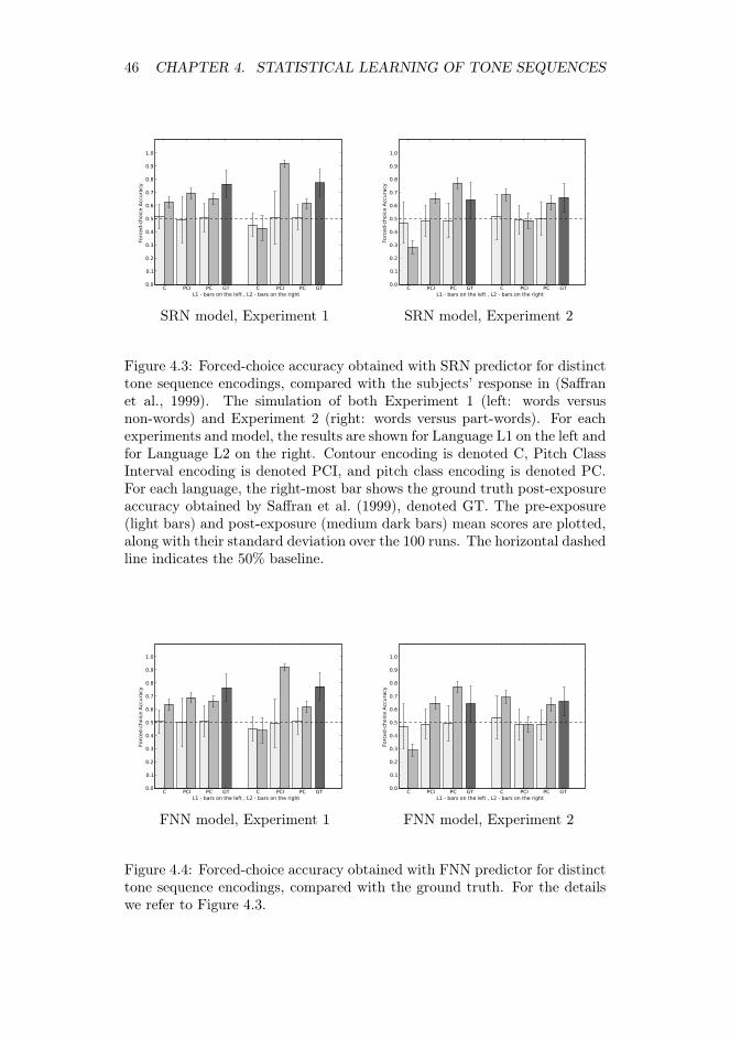
46 CHAPTER 4. STATISTICAL LEARNING OF TONE SEQUENCES
C PCI PC GT C PCI PC GT
L1 - bars on the left , L2 - bars on the right
0.0
0.1
0.2
0.3
0.4
0.5
0.6
0.7
0.8
0.9
1.0
Forc
ed-c
hoic
e A
ccura
cy
SRN model, Experiment 1
C PCI PC GT C PCI PC GT
L1 - bars on the left , L2 - bars on the right
0.0
0.1
0.2
0.3
0.4
0.5
0.6
0.7
0.8
0.9
1.0
Forc
ed-c
hoic
e A
ccura
cy
SRN model, Experiment 2
Figure 4.3: Forced-choice accuracy obtained with SRN predictor for distincttone sequence encodings, compared with the subjects’ response in (Saffranet al., 1999). The simulation of both Experiment 1 (left: words versusnon-words) and Experiment 2 (right: words versus part-words). For eachexperiments and model, the results are shown for Language L1 on the left andfor Language L2 on the right. Contour encoding is denoted C, Pitch ClassInterval encoding is denoted PCI, and pitch class encoding is denoted PC.For each language, the right-most bar shows the ground truth post-exposureaccuracy obtained by Saffran et al. (1999), denoted GT. The pre-exposure(light bars) and post-exposure (medium dark bars) mean scores are plotted,along with their standard deviation over the 100 runs. The horizontal dashedline indicates the 50% baseline.
C PCI PC GT C PCI PC GT
L1 - bars on the left , L2 - bars on the right
0.0
0.1
0.2
0.3
0.4
0.5
0.6
0.7
0.8
0.9
1.0
Forc
ed-c
hoic
e A
ccura
cy
FNN model, Experiment 1
C PCI PC GT C PCI PC GT
L1 - bars on the left , L2 - bars on the right
0.0
0.1
0.2
0.3
0.4
0.5
0.6
0.7
0.8
0.9
1.0
Forc
ed-c
hoic
e A
ccura
cy
FNN model, Experiment 2
Figure 4.4: Forced-choice accuracy obtained with FNN predictor for distincttone sequence encodings, compared with the ground truth. For the detailswe refer to Figure 4.3.

4.4. RESULTS AND DISCUSSION 47
4.4.1 Acquisition of statistical regularities
Inspecting the post-exposure results reveals distinct outcomes dependingon the tone sequence encoding used. We analyzed the results obtained usingindependent samples t-tests when comparing pre and post-exposure scores,and used one-sample t-tests when comparing scores to the 50% baseline .Using the Pitch Class Interval representation, the post-exposure recognitionscores are higher than the baseline for Experiment 1 for both languages(p < 0.001). However, both SRN and FNN models fail in reproducing theresults of the second experiment, because the Language L2 post-exposurescore is lower than the baseline.
The Contour-based representation can not account for the results of Ex-periment 1, because models exposed to Language L2 exhibit a post-exposureaccuracy which is lower than the baseline (p < 0.05). Experiment 2 is notreproduced either: in this case the model population exposed to the Lan-guage L1 exhibits a strong negative post-exposure bias towards this language(p < 0.001). The fact that Experiment 2 involves the comparison of wordsversus part-words explains well the failure in obtaining a good fit using amelodic contour representation: indeed, the words to be discriminated dur-ing the forced-choice task are very similar when projected into a contourrepresentation.
Overall, the most consistent improvement of the post-exposure forced-choice task accuracy for all experiments and languages (p < 0.05 in all cases)is obtained using a Pitch Class representation, that is, a representation wherepitch is not defined with intervals. However, we were not able to reproducethe fact than Experiment 1, because it involves a comparison of words versusnon-words, led to a higher discrimination accuracy than Experiment 2. Inour simulations, the average post-exposure accuracy for Experiment 1 is 65%for Language L1 and 61% for Language L2. For Experiment 2, the averagepost exposure accuracy is 77% for Language L1 and 63% for Language L2.
4.4.2 Influence of used architecture
The first observation to be made concerns the similarity between theresults obtained in Figure 4.3 using the SRN model, and in 4.4 using theFNN model, independently of the encoding used. Our results suggest thatthe SRN model can not take advantage of a longer context when providinga prediction, which may confirm that the task presented in Saffran et al.(1999) can only be solved by means of computing transition probabilitiesbetween successive events.
We have proposed in this paper an attempt towards modelling the acqui-sition of statistical regularities in tone sequences. We have used two ArtificialNeural Network architectures to simulate the general learning trend observedby Saffran et al. (1999). Our results show that the choice of the ArtificialNeural Network architecture has little effect on the post exposure accuracy,which suggests that an extended temporal context is not necessary to modelthis task.

48 CHAPTER 4. STATISTICAL LEARNING OF TONE SEQUENCES
4.4.3 Influence of used representation
We have extended the original experiment with a pre-exposure forced-choice task and observed the outcome of this task with both simulationsand a behavioral experiment. We have found that a bias towards a givenlanguage can appear, which may depend on the tone sequence representa-tion used. This suggests that further studies aimed at investigating tonesequence learning should take into account different representations of thetone sequences.
The simulations based on interval representations such as Pitch Class In-terval or Contour did not consistently account for the experimental results.That is, representations where the information between tones is relative ,enabling shift invariance for instance, do not enable to reproduce the exper-imental results. However, using a tone sequence encoding based on PitchClass, we observe, for all experiments and languages, an increase of the cat-egorization accuracy of words versus non-words and words versus part-wordsin a population of prediction models after they have been exposed to tonesequences containing statistical regularities.
A note on scalability In the simulations presented in this chapter, wehave proposed several alternatives to represent tone sequences. Our modelprovides a prediction of the next tone or interval based on the observationof a limited number of past events. We are interested in scaling our systemin order to process more complex representations of musical events, over anincreased temporal context. That is, we aim at working with a greater setof possible events, while being able to detect patterns of successive events,even if they are separated by more than a few time steps. In this context,it becomes more difficult to train the ANN architectures we have presentedhere in an online learning and prediction setting, where only one trainingepoch is allowed. This is the reason why we will use an alternative learningand prediction model when extending our system in Chapter 6.
4.4.4 Concluding remarks
As a summary of this chapter, we have presented a setup for simulatingthe forced-choice task experiments reported by Saffran et al. (1999) 1. Toachieve this, we have proposed a set of encodings based on absolute pitchvalues, intervals, and contours for representing the tone sequences used inthe experiment, and have used two neural network architectures to imple-ment the learning process that takes place with human subjects. We havefound that the choice of the encoding has a major impact than the networkarchitecture. Contrastingly, as stated in previous chapter, most of the worksfocusing on models of implicit learning for music stimuli use a unique rep-resentation of tone sequences when comparing learning models. Therefore,representation is an important aspect even when using a symbolic represen-tation (Mozer, 1994; Conklin and Anagnostopoulou, 2001; Paiement, 2008).
1. The source code of the simulation framework is available http://emcap.iua.upf.es/downloads/content_final/statistical_learning_experimenter_package.html

4.4. RESULTS AND DISCUSSION 49
In next chapter, we will present approaches to represent musical aspects inaudio signals. Then, we will consider a representation of acoustic eventsthrough time that is not specific to melody in Chapter 6 and will take ad-vantage of the conclusions obtained here to propose a set of representationalternatives. This way, we will be able to study the impact of the represen-tation in the structure learning and expectation processes.


CHAPTER 5Representation and
Expectation in Music: aMid-level approach
5.1 Chapter summary
In Chapter 3 we have introduced models of sequential learning and theirapplications to music modelling. In most cases, these models were appliedto fixed, symbolic representations of musical events. In Chapter 4, we havecompared the use of different symbolic representations in a sequential learn-ing simulation. As our aim is to create a model of listening that can beapplied to a range of musical audio signals, we need to define an interfacebetween symbolic sequence modelling and audio representation approaches.In this chapter, we review approaches to automatic extraction of musical in-formation from musical audio signals that can be used for further sequentialprocessing. Therefore, our system will create symbols that correspond tomusical objects present in a given audio stream, which makes our approachmid-level. Our representation must describe events at a higher level thanthe audio signal itself or quantities directly derived from its time-frequencyanalysis, but should at the same time be less abstract than a score becausewe want it to distinguish objects with different spectro-temporal propertiesand time locations.
First, we review transcription systems that identify musical events fromtheir spectro-temporal properties and their location in time. Then, we showhow audio analysis techniques that involve some predictive behavior can beregarded as simple expectation systems. Finally, we introduce prediction-driven systems and information-theoretic approaches that have been appliedto audio signals. Based on this review, we will present in next chapter amodel that integrates both representation and expectation processes.
51

52 CHAPTER 5. REPRESENTATION AND EXPECTATION IN MUSIC
5.2 Automatic description of signals with attacks,beats and timbre categories
In the last two decades, there has been a substantial amount of workaimed at providing a mid-level description of musical audio. Here, we narrowour presentation to works aimed at producing a mid-level description ofmusical signals in terms of timing and acoustic properties.
5.2.1 Time description: when
First, the incoming audio stream can be described in terms of onsets,that is, the beginning of a musical note or sound. Onset detection is com-monly performed in two steps: first the incoming signal is transformed intoa low-dimensional signal called the detection function. This can be done,for instance, using a bank of temporal filters derived from psychoacousticalknowledge (Klapuri, 1999), deriving a detection function from spectral do-main features (Brossier et al., 2004; Collins, 2004; Duxbury et al., 2003b) orusing supervised learning approaches (Lacoste and Eck, 2007). From this, apeak-picking component takes the detection function as inputs and returnsonset times. The musical stream can also be described in terms of beatswhich characterize the stream periodicity even in the absence of clear per-ceptual attacks. Depending of the approach used, the output of such analysiscan be the average periodicity, the position of the beats, or a location overa finer grained metrical grid. This approach is called beat-tracking or meterestimation, and is presented in Section 5.3.2.
5.2.2 Instrument and melody description: what
Apart from the time dimension, another mid-level description we are in-terested in is the nature of the sounds whose attack is detected. Appliedto a melody, note height would correspond to pitch detection. Unpitchedsounds may be identified using timbre categorization techniques. Both tim-bre and pitch properties may be combined to describe instrument notes ina precise way. The detection of unpitched sounds such as drum soundsand percussive sounds in general has been considered in a variety of MIRsystems. Classification of unpitched sounds has been addressed by Gouyonet al. (2000); Herrera et al. (2002) and was followed by works focusing on thetranscription of percussive excerpts such as drums (Gillet and Richard, 2004;Tanghe et al., 2005a; Yoshii et al., 2005) or beat-box (Kapur et al., 2004;Hazan, 2005c). While these approaches are essentially supervised, becausethey assign a label from a predefined set to the sounds they process, otherworks have proposed unsupervised approaches to categorization of sounds.(Wang et al., 2003; Paulus and Klapuri, 2003; Schwarz, 2004; Jehan, 2005;Hazan, 2005a), assuming a fixed number of timbre categories, or by consid-ering hierarchical approaches Schwarz (2004); Jehan (2005). Indeed, unsu-pervised categorization requires a suitable distance measure between soundsto categorize. Casey (2002); Cano (2006); Pampalk et al. (2008) proposedapproaches focused on similarity measures between sounds. For some of the

5.3. PREDICTION IN EXISTING MODELS OF AUDIO ANALYSIS 53
works presented here (Tanghe et al., 2005a; Hazan, 2005c), causal versionshave been presented, enabling real time implementations.
5.2.3 Combining timbre and temporal Information
Paulus and Klapuri (2003) proposed an unsupervised transcription sys-tem for percussive events that uses both the timbre characteristics of strokesand their temporal features, derived from onset detection and meter estima-tion processes. The first stage on the system groups attacks depending oftheir timbre characteristics. After this stage, each attack is associated to aspecific group, called timbre cluster, in an unsupervised way. Subsequently,timbre clusters are mapped to predefined drum labels by considering therhythmic features of events within each cluster.
On a broader time scale, systems have been proposed to perform auto-matic segmentation of musical pieces, and are called structural segmentationsystems. Examples of structural segmentation systems include (Foote, 1999;Aucouturier and Sandler, 2001; Peeters et al., 2002; Goto, 2003; Ong, 2006).The general idea lies in computing a self-similarity matrix over a descrip-tion of the musical signal. Features include timbre (e.g. MFCC) or chromafeatures. The computation of a self similarity matrix involved in the seg-mentation makes it an inherently batch process.
We have presented an overview of automatic systems that aim to ex-tract musical structures from audio signals. Those structures include eventsonsets, periodicity and metrical structure, and events categories based onspectro-temporal properties. Methods for evaluating the proposed systemshave been proposed, and often require a comparison with data annotated byexperts, known as ground truth. For each specific discipline (e.g. onset de-tection) evaluations of systems from several research teams using a commonset ground truth are organized at MIREX 1. Overall, the MIREX evalua-tions show that even if the accuracy of such systems increases over years,those systems are still error-prone and the issue of automatic description ofmusical audio can not be considered as a solved problem for the time being.Consequently, expectation models applied to audio signals need to take intoaccount the errors introduced by automatic description stages.
5.3 Prediction in existing models of audio analysis
Most of the representation systems introduced above do not incorporateprediction in their processing chain. It is worth noting that the notion ofsignal prediction has long been considered in the audio signal processingfield, at different time scales and levels of abstraction.
First, low-level techniques perform signal prediction at the sample levelor over a short period of time. Then, beat-tracking techniques are based ona higher-level description of the musical signal because they extract infor-mation about its temporal structure, and some of those models can be con-
1. http://www.music-ir.org/mirex/

54 CHAPTER 5. REPRESENTATION AND EXPECTATION IN MUSIC
sidered as time expectation systems. Finally, a system of computational au-ditory scene analysis driven by prediction has been proposed by Ellis (1996).
5.3.1 Audio signal prediction at the sample level
One application of audio signal processing lies in describing the musicalsignal in a more compact form, thus allowing to discard redundant signaldata and reducing transmission costs. One of the techniques that has beendesigned to perform audio signal analysis and compression is Linear Pre-diction Coding (LPC, (Makhoul, 1975)). LPC was originally developed toperform speech signals coding, and has been widely used since then in a vari-ety of applications. The basic idea behind LPC is that speech signals can bedescribed as the result of a simple model of the vocal tract, which contains asource and a filter. To produce vowels, the source uses a sequence of pulses(which originate from the glottis in the vocal tract). To produce consonantsand unvoiced sounds, the source uses a noise-like signal. Then, the sourcesignal is filtered by applying a filter response that is characteristic of a givenphoneme. In the case of speech, 4 formants are usually used to define aphoneme response. Using the source and filter parameters, it is possibleto re-synthesize the signal. Consequently, speech signal can be describedin a compressed form using the source-filter parameters and its residual,which corresponds to the difference between original and the re-synthesizedsignal. LPC performs prediction at the sample level to compute the lin-ear prediction coefficients for a given signal. Further investigations haveproposed predictive models similar to LPC that incorporate psychoacousticknowledge such as Perceptual Linear Predictive analysis (PLP) (Hermansky,1990)) and models that focus on approximating the spectral changes ratherthan the spectrum itself such as RASTA (Hermansky and Morgan, 1994).
Another example of prediction-driven processing is the computation of aspecific onset detection function, know as complex domain (Duxbury et al.,2003b). The complex domain detection function is computed on a spectro-gram by using both magnitude and phase information. For stationary sig-nals, we assume that each spectrogram bin evolves linearly from one frameto the next. It is then possible, for successive frames, to compute an estimateof each incoming bin based on its last values. From this, the error betweenestimated bins and actual bins is computed, resulting in the complex domaindetection function.
Overall, the techniques presented here achieve a form of crude predictionon a low level basis, over a short time period. However, due to the short timescale of the predictions made, these methods can hardly be considered asmodels of of music perception. Following, we consider methods that analyzethe periodicity of musical audio signals over a larger time scale: musicalbeats.
5.3.2 Beat-tracking as Expectation in Time
Beat tracking refers to the process of tracking periodic beat pulses inaudio signals. These pulses correspond to the signal tactus and are often
5.3. PREDICTION IN EXISTING MODELS OF AUDIO ANALYSIS 55
easily estimated by listeners, even if they are non-musicians. From this,it is possible to perform a segmentation of the audio signal or extract itsperiodicity, for instance by computing the average Beats per Minute (BPM).Beat tracking algorithms have been proposed in the last three decades, usinga variety of approaches, and were applied to either symbolic, MIDI or audiodata. Some approaches attempted only to compute the average periodicityof a musical signal without identifying pulses, which is also referred to astempo estimation. Other approaches can additionally identify pulses (Gotoand Muraoka, 1995; Davies and Plumbley, 2005) or extract the finer-grainedmetrical structure of musical signals (Dixon, 1997; Cemgil et al., 2002).
The techniques used for performing beat-tracking range from rule-basedmodels (Povel and Essens, 1985), autocorrelation methods (Davies and Plumb-ley, 2005; Brossier, 2006), oscillating filters (Scheirer, 1998), histogramingmethods (Gouyon and Herrera, 2003), multi-agent systems (Goto and Mu-raoka, 1995; Goto, 2001), probabilistic approaches (Cemgil et al., 2002), andmulti-resolution analysis (Smith, 1996). We refer to Hainsworth (2006) fora detailed review of these approaches.
Here, we focus on approaches that can process audio signals as they canbeen seen as computational models of temporal expectation in the signaldomain. We need to make a distinction between models that process thewhole signal to be analyzed in a batch setting, and causal models that aimat extracting the periodicity, pulse or metrical structure in the audio streamanalyzed so far, and that may be able to locate incoming time regions wheremusical events may occur. As discussed by Hainsworth (2006), methodssuch as oscillating filters make causal processing straightforward, while othermethods can not perform causal processing or need to be adapted to do so,for instance by performing batch processing over a sliding analysis window.
From an expectation modelling viewpoint, a causal beat tracking systemmay be seen as a temporal expectation system. At each point in time, thesystem has to keep track of the most recent pulses and has to predict, basedon the pulse history and the current signal, where the subsequent pulse willoccur. Causal beat tracking is focused on expecting when the next pulseis going to be perceived, without considering which acoustical cues will beassociated to that pulse. That is, they aim to answer the question of whennext events will be heard, and can possibly associate these events to a finer-grained metrical structure. To this extent, beat-tracking approaches mayprovide a useful basis in the context of expectation modelling, and can serveeither as a input of an expectation system or be part of the expectationmodel. However, beat-tracking approaches do not aim at distinguishingacoustical cues in audio signal, and do not inform about what is going tobe heard next. When developing our expectation model in Chapter 6, wewill show how some components of the system are related to beat-trackingapproaches.

56 CHAPTER 5. REPRESENTATION AND EXPECTATION IN MUSIC
Figure 5.1: Block diagram of a prediction-driven computational auditoryscene analysis system, from (Ellis, 1996).
5.3.3 Prediction-driven computational auditory sceneanalysis
The idea of building a system that can represent audio signals in a com-pact form to learn their structure and anticipate forthcoming events has beenintroduced by Ellis (1996). The author proposes a computational frameworkwhere the tasks of representing the acoustic stream and predicting its con-tinuation are closely linked. This model is aimed to provide a more plausiblealternative to standard auditory scene analysis models (Cooke, 1993; Brown,1993). Those models are seen by the author as “data-driven" because theycompute representations of the acoustic stream based on the low-level fea-tures only, without considering in which context these features are computed.Such data-driven approaches make it difficult to deal with ambiguous andnoisy signals. Those ambiguities may be compensated in a model consideringsome knowledge about the signal structure. Furthermore, the author sug-gests that the temporal dynamics of the listening process requires to build anincremental model, which performs analysis in strictly advancing time steps,instead of of performing batch processing of waveforms. A block diagram ofthe presented model is shown in Figure 5.1.
The auditory front-end feeds the system core engine, which is is chargeof reconciliating the low level observations with an ”internal model of thesound-producing entities in the environment“. That is, the engine has toadapt both the world model and the sensory input to find some degree ofagreement between them. The world model is itself based on a representationof the signal, which has be chosen to provide a very general description,intended to deal with the broad auditory environment of human perception.Three acoustic units are used to describe the acoustic environment: noiseunits, tonal units and transients. The system does not take into account

5.3. PREDICTION IN EXISTING MODELS OF AUDIO ANALYSIS 57
Figure 5.2: Diagram of the evolution of various alternative explanationsfrom a simple example involving noise sounds, from (Ellis, 1996). Fromleft to right: a root hypothesis concerning an event occurrence at a giventime gives rise to a tree of possible observations concerning future auditoryobjects.
finer-grained details so that similar sounds with specific differences can bedescribed the same way. This model makes use of a blackboard architecture,which is a functional model of memory and representation. The blackboardprovides a computational framework to allow various competing hypothesesat different levels of abstraction to be considered which gives representationalpower to the system. We show in Figure 5.2 an example of competingrepresentation that can emerge from Ellis system analyzing an audio excerptof a simple experiment from Bregman.
The diagram shown in Figure 5.2 shows the various competing hypothe-ses that can emerge from the analysis of a simple excerpt. An issue raised bythis type of model is the scalability of the system when considering a richerrepresentation. If our aim is to model -even in rough form- the dynamics ofmusical excerpt, we will need to consider a richer representation of events foran extended temporal context. In this case, a blackboard approach wouldquickly face combinatorial explosion issues. Ellis’ model is applied to someanalysis tasks, which includes auditory material such as voices and envi-ronmental sounds. The system is able to re-synthesize its representation ofauditory events, which allows validation by listeners. Ellis has formulateda key modelling principle: an incremental system with a prediction to per-ception feedback loop. However, we need to refine and adapt the modelto accommodate the representation of higher-order structures that may besuitable to represent musical information.

58 CHAPTER 5. REPRESENTATION AND EXPECTATION IN MUSIC
5.4 Information-Theoretic Approaches
We finally review systems that use an information-theoretic approach toaudio analysis and that have proposed a formalism to define prediction inaudio signals. Abdallah (2002) considers redundancy reduction and unsu-pervised learning applied to musical and spoken audio (either waveform orspectral distribution), and reports a set of experiments aimed at defininga base representation of audio signals. Lewicki (2002) follows a similar ap-proach to represent natural sounds. Abdallah also sketches how a musicalsystem may exhibit degrees of suprise in a way rooted in perception andinformation theory. From an information-theoretic viewpoint, the musicalsignal can be viewed as an information source. This source is then trans-mitted to a listener (receiver) through a noisy information channel. As aconsequence of this, the listener perceives both musical structure and noiseassociated to the transmission of the musical content. As such, informationtheoretic models include both the musical signal and the listener into themusic perception model. This provides an alternative account to analysis ofmusical signals by considering the predictability of their structure from thelistener’s point of view instead of merely computing statistics on the musicalsignal itself as it is done in most works listed in Section 5.2 and more gen-erally in MIR systems. According to Abdallah and Plumbley (2009), “thegeneral thesis is that perceptible qualities and subjective states like uncer-tainty, surprise, complexity, tension, and interestingness are closely relatedto information-theoretic quantities like entropy, relative entropy, and mutualinformation.” Pearce and Wiggins (2004) use entropy and cross-entropy toevaluate whether statistical models can learn symbolic monophonic melodies.The entropy rate, denoted H(X|Z), reflects the instantaneous certainty ofstatistical models to characterize the current X observations given Z pastobservations , while cross-entropy applied to test melodies informs about thegeneralization accuracy of a learned statistical model.
Dubnov (2006) introduces a model of transmission of the musical signalover a time-channel. In this model, "The input to the channel is the historyof the signal up to the current point in time, and the output is its next(present) sample." The channel receiver makes a prediction of the upcomingsample based on the history of samples it has received so far. Therefore,it is possible to compare the receiver prediction with the next sample tobe transmitted. The Information Rate (IR) is a measure of how the infor-mation is transmitted from the source to the receiver in the time-channel.Dubnov derives the IR model from this measure, and applies it to scalarand multivariate musical signals. The unidimensional IR case is shown to beequivalent to using a descriptor known as Spectral Flatness (Jayant and Noll,1984). In the multivariate case, the model can process musical signal rep-resented with multi-dimensional audio descriptors. The model is extendedin (Dubnov, 2008), where an additional recurrence analysis component en-ables to detect repetitions in blocks on a larger time scale. In this case, twoparallel processes take place, one focusing on short-term frames of signal tocompute a so-called data-IR, and the other focusing on long-term frames tocompute the model-IR. Applications to audio signals such as natural sounds

5.5. CONCLUDING REMARKS 59
and classical music are presented in (Dubnov, 2006, 2008). Cont (2008) dis-cusses and extends the IR model in his thesis. Abdallah (2008) discusses thevalidity of Dubnov’s IR measure and proposes further information measuresin (Abdallah and Plumbley, 2009), where the authors propose to computethe average predictive information rate, noted I(X,Y |Z) which may be seenas the average rate at which new information arrives about the present andfuture observations X and Y , given past observations Z. In an experimentusing a simple Markov-chain model applied to two Philip Glass minimalis-tic music pieces, the authors show that these measures reveal the structureof the pieces in agreement with the judgment of a human expert listener.However, Abdallah’s model was not tested on representations derived fromaudio signals.
5.5 Concluding remarks
Overall, information-theoretic approaches provide a convenient and el-egant framework to formulate issues such as signal representation and ex-pectation, and may be applied to different representations of musical sig-nals, either in a symbolic form or as audio excerpts. Furthermore, the ideaof deriving a useful representation of musical signals in a purely unsuper-vised way - instead of crafting specific representation algorithms for specifictasks - is appealing. However, more work is needed in this area to give re-searchers ways of extracting musical structure as those found in state of theart MIR systems. As an alternative to pure MIR-centered and Information-theoretic systems, we will propose in next chapter a hybrid approach. Sometypical components from MIR systems will be used to provide a mid-levelrepresentation of audio events, those events will in turn be processed inan information-theoretic fashion to further organize them and enables theirprediction.


CHAPTER 6The What/Whenexpectation model
6.1 Chapter summary
Our model of music expectation is aimed at combining audio signal rep-resentation and the generation of future occurrences in this representationwithin a single framework. A causal system to represent a stream of musicinto musical events, and to generate further expected events, is presentedhere. Starting from an auditory front-end which extracts timbral and tem-poral features such as onsets and beats, a categorization process (eithersupervised or unsupervised) builds and maintains a set of symbols aimed atrepresenting musical stream events using both timbre and time descriptions.The time events are represented using inter-onset intervals relative to thebeats. We propose and compare three ways of combining time and timbredimensions regarding the prediction of the next event. Several alternativesto timbre and timing description, cluster estimation and assignments areconsidered.
These symbols are then processed by an expectation module using Pre-dictive Partial Match, a multiscale technique based on N-grams. To char-acterize the ability of the system to generate an expectation that matchesboth ground truth and system transcription, we introduce several measuresthat take into account the uncertainty associated with the unsupervised en-coding of the musical sequence. The system is evaluated using a database ofannotated drum recordings. We compare three approaches to combine tim-ing (when) and timbre (what) expectation. The applications of this models,including visualization and sonification of the expectation, are presented inChapter 7.
61

62 CHAPTER 6. THE WHAT/WHEN EXPECTATION MODEL
6.2 Motivation
Our main focus lies in integrating a learning system which can constantlylearn aspects of the structure of musical audio signals while it listens to mu-sical events, in a way that is inspired by cognitive principles. We propose acausal and unsupervised system that learns the structure of an audio streamand predicts how it will continue. Our system uses concepts and approachesfrom a variety of research topics: automatic music transcription, unsuper-vised learning and model selection, and symbolic statistical learning. Amid-level representation of the signal is constructed as a discrete sequenceof symbols representing time dependencies between events and timbre prop-erties. A prediction of the subsequent symbols can then be provided, fromwhich the system can then predict the nature and the timing of the next mu-sical event. As such, the system prediction algorithm is symbolic, but thesystem is responsible of producing a symbolic representation of the musicalstream in an unsupervised manner (i.e. the symbols are based on acousticinformation).
From a general viewpoint, we assume a musical sequence as being asuccession of musical events with intrinsic properties (e.g. pitch, loudness,timbre) which are heard at a given time. While the musical sequence isattended, timbre and timing patterns perceived so far (among other musicalinformation that is not considered in this paper) can be used to providea prediction of the next musical event to be heard. The prediction canbe made over several dimensions, e.g. the timbre properties of the nextevent to be heard (what) or the temporal location of the next event (when).Distinct strategies may be used by listeners to combine predictions alongthese dimensions. Even tough in the case of timbre recent evidence pointsto the possibility that certain timbre dimensions (e.g., attack slope, spectralcentre of gravity, etc.) could be processed separately (Caclin et al., 2006) wewill consider timbre as a nonseparable dimension to be used for predictingevents. From the physiological literature, it seems to be a separation betweenthe circuits dealing with the detection of violations of musical expectancies orpredictions (in the ventrolateral prefrontal cortex), and the circuits dealingwith the processing of perceptual objects and their monitoring in workingmemory in the dorsolateral prefrontal cortex and posterior parietal cortex(Sridharan et al., 2007).
In addition, we may assume a functional and physiological separation be-tween sequential processing (related to musical syntax and grammar) whichcould take place in Broca’s area (Maess et al., 2001) and the processing oftiming information, which could be happening at the right temporal audi-tory cortex and superior temporal gyrus (Peretz and Zatorre, 2005)). Fromthese physiological considerations we could address the prediction of whatand when dimensions as two independent processes which may be modeledwith two independent predictors.
However, from the Auditory Scene Analysis (Bregman, 1990) point ofview, sound events may be separated into different auditory objects (audi-tory stream segregation) or assigned to a single auditory object (auditorystream fusion). This depends on the intrinsic properties of the musical events

6.3. OVERVIEW OF THE SYSTEM 63
(e.g. timbre, pitch) and the timing of the events. If auditory stream inte-gration takes place, each event may be described as how it differs from thepreceding event in terms of timbre and timing. In this sense, the what andwhen dimensions might be merged into a unique dimension, which wouldbe modeled with a unique next-event predictor. Finally, if auditory streamsegregation takes place, a different representation of the events has to beconsidered. In a perceptual experiment (Creel et al., 2004), while the statis-tical regularities between nonadjacent tones were hardly learned when themusical sequence contained events which were similar in pitch or timbre,these regularities could be acquired when the temporally nonadjacent eventsdiffered in pitch range or timbre. Therefore, if a musical sequence can beperceptually segregated into separate timbre streams, the temporal depen-dencies between events might be computed (to a certain extent) from theseparate timbre stream rather than from the temporally adjacent elements.This could be modeled by considering each segregated stream as a separatedimension which would be modeled with a stream-specific timing predic-tor. The system we present in this chapter enables us to implement thesethree strategies and compare them empirically using a database of annotatedsequences of percussive events.
6.3 Overview of the system
The system has the following modules: feature extraction, dimensionalityreduction, and next event prediction. These components, all of which runsimultaneously when the system is following a musical stream, are shown inFigure 6.1. First, the feature extraction module is the audio front-end, whichextracts timbre descriptors, onsets and beats from the incoming signal. Thismodule is based on the Aubio library (Brossier, 2006). Each extracted hitis encoded in the dimensionality reduction module based on both time andtimbre description, following an unsupervised scheme. Therefore, we obtaina symbolic representation of the incoming events, to be used by the nextevent prediction module.
6.4 Low and Mid-level Feature Extraction
6.4.1 Analysis Settings
The audio stream is analyzed using a window size of 1024 samples (23ms using a sampling rate of 44 KHz) with 50 percent overlap. We apply aHamming window before computing the Fast Fourier Transform (with thesame window size) to perform spectral analysis.
6.4.2 Temporal detection
Onsets are extracted as events are presented. Optionally, beat locationsare extracted, and combined with onsets to produce a tempo-independenttiming characterization between successive events. We present the methodsused for achieving both onset detection and beat tracking tasks.

64 CHAPTER 6. THE WHAT/WHEN EXPECTATION MODEL
FeatureExtraction
timbre descriptors
onsets
beats
DimensionalityReduction
event timbre class
event IOIclass
Next EventPrediction
next eventtimbre class
next IOI class
Audio to Symbolic
Symbolic to Audio
Figure 6.1: System diagram. Feedforward connections (left to right) create astream of symbols to be learned. Feedback connections (right to left) enablesymbolic predictions to be mapped back into absolute time. IOI refers toInter-Onset Interval, as explained in the next section.
Onset detection We compare different onset detection techniques thatare available in the Aubio library. The methods we compare are the follow-ing:
– High-Frequency Content (HFC, (Masri, 1996)), obtained by summingthe linearly-weighted values of the spectral magnitudes
– Complex domain (Duxbury et al., 2003a), obtained by observing thefluctuation of the spectrum in the complex domain, thus taking ad-vantage of both phase and magnitude.
– Dual: a hybrid function which combines the complex domain functionwith a function based on the KL-divergence.
Details and evaluation for these algorithms are available in (Brossier, 2006).
Beat tracking Beat tracking can be applied to provide time anchors fromwhich it is possible to describe inter-onsets intervals in a beat relative fashion.This would enable the system to create a tempo-invariant representation oftime. The tempo detection algorithm is based on (Davies et al., 2005). Thisalgorithm is based on the autocorrelation of the onset detection function. Acomb filter is applied to the resulting autocorrelation function, leading to anhistogram of the period candidates. The histogram peak is then selected asthe detected period, denoted Period(t).
6.4.3 Inter Onset Intervals Characterization
We propose here alternatives to characterize timing relations betweenevents. As an outcome of the temporal detection, the duration betweensuccessive events can be measured. These intervals can be seen as an absolutedifference of onset times, or as beat-relative difference.

6.5. EVENT QUANTIZATION 65
Inter Onset Interval If an onset occurs at time tcurr, and the previousonset has occurred at time tprev we can derive the absolute Inter OnsetInterval (IOI) as:
IOI(t) = tcurr − tprev (6.1)
Beat-Relative Inter Onset Interval Based on this, for each new event,the beat-relative inter-onset interval (BRIOI) is computed as follows:
BRIOI(t) =IOI(t)
Period(t)(6.2)
where IOI(t) refers to the inter-onset interval between the current eventonset and the previous onset, and Period(t) refers to the current extractedbeat period.
Cluster-Wise Inter Onset Intervals Each incoming event belongs to atimbre class. In Section 6.5 we propose an unsupervised approach to assigna timbre symbol to incoming events. This makes it possible to computeIOI between events that belong to the same timbre category, instead ofcharacterizing IOI between successive events of distinct timbre classes.
Beat Relative Cluster-Wise Inter Onset Intervals can be computedsimilarly to BRIOI.
6.4.4 Timbre Description
We use 13 Mel-Frequency Cepstrum Coefficients (Davis and Mermelstein,1980). We have implemented the MFCC in the Aubio library (Brossier, 2006)following Slaney’s MATLAB implementation, using 40 filters. We computethe median of each coefficient over a 100 ms window starting from the onsetframe, in order to represent both attack and tail of the detected event. Thevalue of 100 ms is chosen as a tradeoff allowing to either represent short,percussive sounds or longer sustained sounds.
6.5 Event quantization in the time and timbre space
In the dimensionality reduction and event quantization stage, our systemassigns detected events to discrete time and timbre categories, thus creatinga symbolic description of the audio stream. This is done by applying dimen-sionality reduction and clustering techniques, as shown below. Therefore,the output of this stage a set of cluster assignments corresponding to timbreand timing properties of the detected events. We will see in Section 6.6.2alternatives to recombine these cluster assignments to obtain the desiredsymbolic representation.

66 CHAPTER 6. THE WHAT/WHEN EXPECTATION MODEL
6.5.1 Bootstrap step
Before starting to effectively encode and expect musical events, the sys-tem accumulates observations and therefore acts having a short-term mem-ory buffer to gather statistics based on the incoming hits. During this accu-mulation period, the system does not provide any prediction regarding thefuture events. The processes involved here are (a) feature normalization,(b) Principal Component Analysis (PCA) for dimensionality reduction and(c) estimation of the number of clusters, for both timbre features and IOI.While (a) and (c) are always performed, (b) is only applied to the timbrefeatures, and it is optional.
Bootstrap feature preprocessing– Feature normalization: we normalize the accumulated timbre descrip-
tors and IOI so that they have zero-mean and unit variance. The initialdistribution of parameters is stored so that any normalized instance canbe mapped back into its initial feature space.
– PCA: A PCA can be performed on the bootstrap normalized timbrefeatures. In this case, instead of choosing the target dimensionality,we choose the desired amount of explained variance of the projectedset compared to the original set.
The bootstrap information is stored as it enables to subsequently per-form normalization and dimensionality reduction on new data (Figure 6.1,left to right connection), or to expand and apply inverse normalization tothe projected data (Figure 6.1, right to left connection). Additionally, wealso store the normalized and projected short-term history, which is used toestimate the number of clusters to work with. This step is presented in thenext paragraph.
Evaluating the number of symbols The number of clusters to representboth IOI and timbre events influences the performance of the system and hasto be chosen carefully during the bootstrap step. We perform first a clusterestimation using a grid of Gaussian Mixture Models with diagonal covariancematrix, trained with the Expectation-Maximization (EM) (Dempster et al.,1977) algorithm, following a voting procedure derived from (Cournapeau,2006).
If our maximum number of clusters is fixed to M , we need to performmodel fitting for all the cluster values from 1 toM and select the best modelby taking into account both likelihood to the data and model complexity. Ad-ditionally, for each cluster number, we run R independent processes, whichprovides a better robustness to our estimation. Therefore, we create an es-timation grid in which R ∗M , where M is the maximum number of clusterswe allow, and R is the number of independent runs. Each column of the gridrepresents R models with an increasing number of clusters, from one to M .We train each grid model with EM, using 20 iterations. Once the grids aretrained we proceed to the model selection step by computing informationcriteria as explained below.
6.5. EVENT QUANTIZATION 67
Information criteria for model selection Each grid model can be de-scribed with the following parameters. First, the maximized likelihood, de-noted by L, is a quantitative measure of how the trained model fits thedata. The number of free parameters, K, measures how complex the modelis. The number of samples N is the number of instances present in theshort-term history (see previous paragraph). Different information criteria(IC) have been used in the model selection literature, which are describedbelow. First, the Bayesian Information Criterion (BIC) (Schwarz, 1978) isdefined as follows:
BIC = −2 ln(L) +K ln(N) (6.3)
The BIC strongly penalizes complex models. Models with few parametersand which maximize the data likelihood minimize the BIC. Akaike (1974)proposes another information criterion which penalizes less the model com-plexity, but does not take into account the amount of available data.
AIC = 2K − 2 ln(L). (6.4)
In Section 6.7, we will compare the performance of the system wheneither BIC or AIC are used to determine the number of clusters in the data.To decide the final number of clusters we compute the median over thecross-runs:
K = median1≤i≤R(argmin1≤j≤M (IC)) (6.5)
As an outcome, the estimated number of timbre and IOI clusters is notedKTimbre and KIOI respectively.
6.5.2 Running state
Once the clusters have been estimated for timbre features and BRIOI, wehave to generate cluster assignments for incoming instances and update theclusters to take into account these new instances. To achieve this, we use anonline K-means algorithm, with each cluster mean vector being initializedby the GMM model selected at the end of the bootstrap step. A cluster isassigned to each instance x following:
kx = argmin1<k<K ||x− µk|| (6.6)
where µk is the k-th cluster mean. Then the mean of the assigned cluster isupdated following:
∆µkx= η(x− µkx
) (6.7)
Here η is the learning rate, which controls how much each new instanceinfluences the mean update of its assigned cluster. Values near zero have theeffect of quantizing the incoming instance to the cluster mean, while valuesnear one tend to shift the cluster mean towards the instance assigned toit. We have experimented with values comprised between 0.1 and 0.9, andhave also implemented an optimal learning rate schedule, following (Bottou,2004). In this latter case, the learning rate depends on how many instancesa given cluster centroid represents.

68 CHAPTER 6. THE WHAT/WHEN EXPECTATION MODEL
Then the optimal learning rate can be computed as:
ηoptk =1
nk(6.8)
where nk represents the current number of data points in cluster k.We illustrate the overall timbre encoding process in Figure 6.2 using a
commercial drum’n bass pattern (Audio.1). The normalized distance in-volved in the cluster assignment step is obtained at the end of the bootstrapstep. A principal component analysis has been used to project the internaltimbre description into two dimensions.
-3 -2 -1 0 1 2 3 4
First Component
-4
-3
-2
-1
0
1
2
3
Seco
nd
Com
pon
en
t
Figure 6.2: Timbre clusters assigned to each event after exposure to a com-mercial drum’n bass pattern (Audio.1). The timbre descriptors are MFCC.Crosses, squares and triangles represent points assigned to a specific timbrecluster.
Finally, we show in Figure 6.3, the BRIOI cluster assignments whenprocessing the same excerpt. The figure shows the raw, unclustered BRIOIhistogram (bottom), and the histogram of clustered BRIOI (top), i.e. inwhich each BRIOI event has been substituted by the current mean of itsassigned cluster. We can see that the IOI clustering process performs a kindof "soft" quantization of the raw IOI values.
6.6 From representation to expectation
6.6.1 Multi-scale N-grams
The prediction module has to deduce the most likely future events basedon the sequence observed so far. We treat the incoming encoded signal as

6.6. FROM REPRESENTATION TO EXPECTATION 69
0.5 1.0 1.5 2.0 2.5 3.0 3.5 4.0 4.5 5.0
Clustered Inter-onset intervals (quarter duration)
0102030405060708090
0 1 2 3 4 5 6
Unclustered Inter-onset intervals (quarter duration)
0
10
20
30
40
50
60
Figure 6.3: Unclustered and clustered BRIOI histograms after exposure toa commercial drum’n bass pattern.
a sequence of symbols and use a symbolic expectation algorithm. In thiswork, we use the Prediction by Partial Match (PPM) (Cleary and Witten,1984) algorithm. PPM is a multiscale prediction technique based on N-grams, which has been applied to lossless compression and to the statisticalmodelling of symbolic pitch sequences (Pearce and Wiggins, 2004). In N-gram modelling, the probability distribution of the next symbol is computedbased on the count of the sub-sequences preceding each possible symbol.
The probability distribution of the next symbol ei, where 1 ≤ i ≤ K,given the context sequence ei−1(i−n)+1 is:
p(ei|ei−1(i−n)+1) =
{α(ei|ei−1(i−n)+1) if c(ei|ei−1(i−n)+1) > 0
γ(ei−1(i−n)+1)p(ei|ei−1(i−n)+2) if c(ei|ei−1(i−n)+1) = 0
where c(ei|ei−1(i−n)+1) is the number of counts of each symbol ei followingthe subsequence ei−1(i−n)+1. The symbol counts, given each possible subse-quence of size n, are stored in a transition table containing Kn rows and Kcolumns. When a symbol has not appeared after ei−1(i−n)+1, the model per-forms a recursive backoff to a lower-order context. Here we use a PPM modelwith escape method C (Moffat, 1990) and update exclusion, which providesa reasonable tradeoff between accuracy and complexity. In addition, γ andα are defined as follows:
γ(ei|ei−1(i−n)+1) =t(ei−1(i−n)+1)∑
K c(ei−1(i−n)+1) + t(ei−1(i−n)+1)(6.9)
α(ei|ei−1(i−n)+1) =c(ei|ei−1(i−n)+1)∑
K c(e|ei−1(i−n)+1) + t(ei−1(i−n)+1)(6.10)

70 CHAPTER 6. THE WHAT/WHEN EXPECTATION MODEL
In Equations 6.10 and 6.9, the quantity t(eji ) is the number of differentsymbols which have appeared in the subsequence eji , j > i.
6.6.2 Combining timbre and time: expectation schemes
The PPM predictor presented above produces an expectation of the nextsymbol to be observed given the observed context. We are interested inproviding two predictions, concerning the timbre category and IOI categoryof the future event to be perceived. We propose to compare three expectationschemes whose graphical models are illustrated in Figure 6.4.
Figure 6.4: Graphical models of three schemes for combining what and whenprediction.
Independent what/when prediction scheme Two independent PPMsymbolic predictors are used. The random variables Timbre and IOI arethus considered independent.

6.6. FROM REPRESENTATION TO EXPECTATION 71
Joint prediction scheme After the bootstrap step, the number of timbreand IOI symbols KTimbre and KIOI has been determined. From this, a newset of symbols denoted Timbre⊗IOI is created. This set contains exhaustivecombinations of timbre and IOI symbols, therefore it has KTimbre ∗ KIOI
elements. This approach can lead to high memory requirements if KTimbre ∗KIOI becomes high. In this case, a unique PPM predictor is used to predictthe symbol Timbre⊗ IOIt+1.
When|what prediction scheme Each timbre cluster is associated witha specific cluster-wise IOI symbol predictor (see Section 6.4.3). This meansthat for each timbre cluster, there is a predictor which provides a guess ofwhen an event belonging to the same timbre cluster will appear.
6.6.3 Scheme-dependent representation architecture
Depending of the expectation scheme used, the representation layer pro-cesses need to be adjusted to create a relevant set of timbre and/or timesymbols. Here, we show the building blocks of the representation layer forthe following schemes:
– Joint and independent scheme: both timbre and time symbols arecreated to either serve as input to two independent predictors (inde-pendent scheme) or be recombined into a set of combined timbre/timesymbols (joint scheme) We show a block diagram of this configurationin Figure 6.5.
– When|what prediction scheme: IOI between events of the same timbrecategory are categorized by category-wise online K-means processes.Symbols are then given as input to a set of IOI symbol predictors, onefor each category. The representation block diagram for this configu-ration is shown in Figure 6.6.
Timbre Descriptors
Onsets
Beats
IOI
Attack Descriptors
BRIOI
Audio In
NormOnline K-Means
IOI Distance
Online K-Means
TimbreDistance
PCANorm
Timbre Symbol
IOISymbol
Figure 6.5: Block diagram of the representation layer used for independentand joint expectation schemes. Directed arrows represent the data processingflow, thick boxes represent processes that are initialized during the bootstrapstep. Additionally, the distances involved in the categorization process areshown with rounded boxes.

72 CHAPTER 6. THE WHAT/WHEN EXPECTATION MODEL
Figure 6.6: Block diagram of the representation layer used for when|whatscheme. In this example, the number of timbre clusters is three, as resultof the estimation in the bootstrap step. Directed arrows represent the dataprocessing flow, thick boxes represent processes that are initialized duringthe bootstrap step. Additionally, the distances involved in the categorizationprocess are shown with rounded boxes.
6.6.4 Unfolding time expectation
Based on the symbolic expectation generated, we can produce a timbreand BRIOI symbol expectation. From this, we apply an inverse normaliza-tion of the mean of the chosen BRIOI cluster and scale it to the currentextracted tempo to obtain the absolute time position of the expected on-set for the expected timbre cluster. Following we show in Figure 6.7 bothtranscription and expectation timelines obtained during exposure to a drumexample. Here KTimbre equals 3. While the beginning of the expectationtimeline only contains events of timbre cluster #1 with random inter onsetintervals, after a few seconds events from timbre cluster #3 start to be pre-dicted following the transcription pattern. Then, the IOI pattern involvingtimbre cluster #1 events is learned, progressively followed by the timbrecluster #2 pattern.
6.7 System evaluation
In this section we present an evaluation of the system using a databaseof drum patterns. We first introduce a range of performance metrics for this

6.7. SYSTEM EVALUATION 73
Figure 6.7: Comparison of transcription (top) and expectation (bottom)during exposure to an artificial drum pattern. Vertical colored lines indicatedetected and expected events belonging to different timbre clusters. Thevertical axis indicates time, after the bootstrap step has been performed.
task. We then present an experiment involving predictive learning of drumpatterns.
6.7.1 Performance metrics
Our system produces an on-line transcription of the incoming audiostream and estimates, for each run, the optimal number of clusters to beused to produce a transcription. The transcription is used in turn to pro-duce an expectation timeline which contains the same number of clustersthan the transcription. Consequently, by using a database of annotatedaudio excerpts, several comparisons can be made. First, the transcriptionaccuracy can be computed. Then, the transcription and the expectationproduced by the system can be compared, without taking into account theannotations. To this respect, it would be desirable to know about violationsof expectancies when human listeners learn a set specific musical patterns.Unfortunately such experiments have not yet been performed, and wouldrequire a careful choice of rhythms and acoustic stimuli. Finally the expec-tation timeline can be compared to the ground truth annotations. In thissection, we present the performance metrics we use to achieve all these steps.
Comparison with the ground truth
Precision and recall applied to unsupervised transcription In thecontext of unsupervised transcription it might be useful to compare a se-quence of events transcribed in an unsupervised way with a ground truth

74 CHAPTER 6. THE WHAT/WHEN EXPECTATION MODEL
annotation, where each ground truth event belongs to a fixed set of labels.If the sequence transcribed is labeled we can evaluate the analysis derivedfrom the event detection and unsupervised clustering processes. We use ameasure introduced in (Marxer et al., 2007) and (Marxer et al., 2008) thatis designed to evaluate clustering when the mapping between the referenceclasses and estimated clusters is unknown. The confusion matrix is firstconstructed by using the onset matching technique presented by Brossier(2006) adapted to multiple classes of onsets. Let us consider C the numberof ground truth classes and K the number of clusters. We write nc,k thenumber of co-occurrences of class c and cluster k, nc the total number ofoccurrences of class c. Then we can express the precision and recall as:
P (c, k) =
{1−
∑1≤i≤C,i6=c ni,k∑1≤i≤C,i6=c ni
if C > 11 otherwise.
(6.11)
R(c, k) =
{ nc,k−1nc−1 if nc > 1
1 otherwise.(6.12)
The pairs of precision and recall of each cluster are integrated to achieveprecision and recall measures per class. The integration is performed by do-ing a weighted average of the precision and recall values of the co-occurrences,among all occurrences of class c. The total precision and recall measures arethe weighted sums of the per-class measures.
We will use P andR to evaluate the transcription and prediction accuracyof our system. When comparing the transcription timeline with the groundtruth we will call the precision measure Transcription Incremental Preci-sion (TIP ) and the recall measure Transcription Incremental Recall (TIR),and derive from these measures the Transcription Incremental F-Measure(TIFM). When comparing the expectation timeline with the ground truthwe will use the terms Expectation Incremental Precision (EIP ) for P andExpectation Incremental Recall (EIR) for R, and from these measures wederive the Expectation Incremental F-Measure (EIFM)
Other useful metrics In addition to the measures defined above, wealso consider a simple metric which compares the complexity of the systemrepresentation with the timbre complexity of the attended signal. This canbe done straightforwardly by computing the class to cluster ratio as follows:
CCR =KTimbre
CTimbre(6.13)
where CTimbre is the number of different annotated timbre labels for thisexcerpt, and KTimbre has been estimated at the end of the bootstrap step(see Equation 6.5).
Finally, it may happen, if the sensitivity of the system is low, that thebootstrap step leads to an estimate of timbre clusters equal to one. This isclearly not desirable in the context of evaluating a system which combinestime and timbre dimension. For this reason, we introduce another statistic,which we name P1, and define as the percentage of runs in which the estimateof clusters led to one timbre cluster.

6.7. SYSTEM EVALUATION 75
Comparing expectation and transcription
Comparing expectation and transcription timelines is easier than a com-parison against the ground truth, mainly because both timelines share thesame cluster representation. That is, the list of transcribed event onsets in-dexed by cluster n can be compared directly to the the list of expected eventonsets indexed by cluster n by using onset detection related measures. Wecould compute the average F-measure by comparing both transcribed andexpected timbre cluster onset times for each of the timbre clusters. How-ever, such metrics cannot be considered here because of the variability ofthe unsupervised encoding we use. That is, the encoder provides a numberof timbre clusters that is an approximation of the number of instrument oracoustic categories. For instance, the encoder can return an estimate of fivetimbre clusters for an excerpt containing three instruments. Consequently,during the running state, few of these clusters are indeed used, because a vastmajority of the incoming instances are assigned to a subset of the estimatedclusters (in the example, three of the five estimated clusters). As a result,the underrepresented clusters are likely to return very low F-measures, whichmay in turn affect the average computed F-measure.
In (Hazan et al., 2007) we have proposed to use the weighted averageF-measure, which is defined as follows:
WFM =
Kt∑i=1
wiFi (6.14)
where Kt is the number of timbre clusters, each wi is obtained by dividingthe number of onsets assigned to cluster i by the total number of onsets, andFi is the standard F-measure between onsets assigned to cluster i, with +/-50ms tolerance windows. The individual cluster-wise F-measures involved inthe resulting average computation are weighted by the proportion of eventsappearing in that cluster. This enables us to reduce the contribution ofunused or scarcely-used timbre clusters.
Information-theoretic viewpoint: expectation entropy
For each incoming event, the entropy of each expectation can provide in-formation about the certainty of the returned prediction. For each predictor,the entropy can be computed as follows:
H(p) = −∑
1≤i≤K
p(ei)log2p(ei) (6.15)
where p(ei) is the next event estimated probability distribution over the setof possible symbols K. For each detected event, a number of expectationscan be generated depending on the expectation scheme. The variation ofthe prediction entropy signal may give additional information regarding thestructure of the attended stream. We will go back to this aspect whenpresenting the results in Section 6.7.7.

76 CHAPTER 6. THE WHAT/WHEN EXPECTATION MODEL
6.7.2 Experiment: Loop following
Based on the performance metrics introduced above, we present an em-pirical evaluation based on a database of drum loops. These drum loopsprovide a good evaluation material because they contain strokes with dif-ferent acoustic properties, which are organized through time patterns ofvarying complexity. The task, material and system settings are presented,then we present and discuss the results. The task we propose to simulate isthe following: the system is initialized and it does not access any previouslytrained models; it is exposed to a drum loop repeated several times; oncethe system has accumulated enough information to perform the bootstrapstep and both timbre and IOI symbols are defined, the transcription andexpectation timelines are produced. From these, we can compute, at eachloop repetition, the statistics presented in previous section.
Material We have selected a subset of audio recordings from the ENST-Drums database (Gillet and Richard, 2006). We use polyphonic drum loopsplayed by one drummer, namely drummer #2 in the database. The databaseconsists of 49 drum excerpts (called phrases in the database) of 9 differentstyles, for a total of 5627 events. Most of the database patterns have a dura-tion of approximately 10 seconds, that is, slightly more than the time neededto perform the bootstrap computation. In order to observe the learning dy-namics of the system, we need to work with longer excerpts. We thereforehave edited and looped the original signals 2, 4, 8 and 10 times, dependingon the experiment.
Annotations preprocessing As stated by Gillet and Richard (2006),each drum excerpt was annotated following a semi-automatic process. Forinstance, each cymbal has a distinct label and there is a distinction madebetween open hi-hat and closed hi-hat. Because each drum excerpt wasrecorded using 8 microphones, simultaneous strokes were also precisely anno-tated. The average number of timbre labels present in each excerpt includedin our subset is 5.5.
Because our system is processing the input stream with a fixed framerate (the time precision is 11.6 ms) and performs timbre clustering as ifthe input was monophonic, we decide to apply the following ground truthpreprocessing. If consecutive onsets follow one after the other so that theyare in the same analysis frame, we merge the annotated labels into one jointlabel and keep as onset time the first onset of the consecutive attacks.
Experimental setting The system is designed to learn in a causal way,therefore it may learn more accurately when being exposed to the excerptsseveral times: this is why we have experimented with a number of repetitionsof the basic loop of 2, 4, 6, and 8. The other parameters (e.g. onset detec-tion threshold, model selection information criterion, timbre PCA explainedvariance, next event predictor context size) are varied for comparison pur-poses as explained below. Unless explicitly notified, the default parameterswe use are listed in Table 6.1.

6.7. SYSTEM EVALUATION 77
Parameter ValueDescriptor set MFCCOnset detection threshold 0.6Onset detection Method DualPCA explained variance 0.6# Bootstrap events 40Maximum N-gram order 2Model Selection Criterion AICOn-line K-means η ηopt
Table 6.1: Default parameters used for simulations
6.7.3 Results
This section presents the results of the evaluation whose details are pre-sented in the previous section. Because our expectation system is made ofseveral components, we first present the evaluation of these components inisolation. Then, we provide an overall system evaluation based on the systemtranscription and expectation accuracies.
6.7.4 Evaluation of system components
It is possible to evaluate some of the system components by providingthem as input the data which can be extracted from the ground truth. Giventhe ground truth annotations (i.e. onset times and labels), we can evaluatesome processing stages of the system, such as onset detection and timbreclustering, in isolation. Other stages cannot be directly evaluated with theannotations. The ENST-Drum data is not beat-marked, consequently wehave not performed an evaluation of the beat tracking component, and referto Brossier (2006) for an evaluation of this component. Also, some compo-nents rely on a symbolic representation of time. This is the case of the IOIclustering component which provides IOI cluster labels as output, and thenext-event prediction component, which uses IOI cluster labels as input andoutput. Concerning the symbolic expectation component, the PPM stagehas been evaluated using symbolic pitch sequences by Pearce and Wiggins(2004). In our case, the symbolic representation we are going to feed to thePPM will possibly be noisy, due to event detection and clustering errors.However, we are interested in evaluating this component under this noisyrepresentation rather than in isolation as shown is Section 6.7.5. We firstpresent the results of the onset detection and timbre clustering stages, whenevaluated against ground truth annotations.
Onset Detection
We have first performed an evaluation of the onset detection componentby comparing the detected onsets with ground truth annotations, for threeonset detection functions labeled complex, dual, and hfc. We refer to Sec-tion 6.4.2 for an overview of these methods. For each method, we have varied

78 CHAPTER 6. THE WHAT/WHEN EXPECTATION MODEL
the threshold of the peak-picking stage. We used the database presented inSection 6.7.2, and found that the best configuration was associated withthe dual detection function and a peak-picking threshold value of 0.6. Thecorresponding F-measure is equal to 0.76, and is comparable to the resultsobtained by the dual detection function in MIREX 2006 1. However, theresults are lower than those of more recent onset detection techniques evalu-ated on drum solos in MIREX 2009 2. Nevertheless, here we aim at showingthat the possibly noisy representation can still be exploited in further stagesof the system. In next section, we study how the automatic detection stageaffects the timbre clustering process.
Timbre Clustering
We report here the results obtained when evaluating the timbre clusteringcomponent. We propose two evaluation settings in which the inter-onset re-gions processed by the timbre clustering component are obtained differently.In the first configuration, the regions correspond to the onsets provided bythe ground truth of the ENST-drums database. Thus we evaluate the timbreclustering component in isolation. In the second configuration, the audio re-gions correspond to the onsets computed by the onset detection component,consequently we evaluate the overall accuracy of the combination of onsetdetection and timbre clustering components.
The timbre clustering accuracy is largely influenced by the outcome ofthe bootstrap process, in which a PCA can be trained on the bootstrap data,and the estimation of the optimal number of clusters is performed. For thisreason, we vary the PCA desired explained variance between 0.1 and 0.8 (ordo not perform PCA at all), and the information criterion to be used (eitherBIC or AIC).
Following, we present the mean transcription statistics obtained whenvarying these parameters. For each run, we report the Transcription Incre-mental F-measure (TIFM), the class to cluster ratio (CCR) and percentageof estimates, and the percentage of estimates leading to one timbre cluster(P1). In Table 6.2 the onset times from the ground truth annotations areused, which enables to appreciate the accuracy of system based on a per-fect onset detection process. In Table 6.3, the onset times are extractedautomatically.
On the one hand, the results corresponding to ground truth onsets showthat the combination of the amount of data compression (controlled by thePCA desired variance) and the information criterion play an important rolein the outcoming timbre representation. In all cases, the TIFM lies between0.509 and 0.572. The TIFM average for runs based on AIC (respectivelyBIC) is 0.551 (respectively 0.536). However we see that AIC-based estima-tion leads to a better estimation (mean CCR 0.753) than the BIC-basedestimation (mean CCR: 0.514). If both criteria tend to estimate less clus-
1. http://www.music-ir.org/mirex/2006/index.php/Audio_Onset_Detection_Results
2. http://www.music-ir.org/mirex/2009/index.php/Audio_Onset_Detection_Results:_Solo_Drum

6.7. SYSTEM EVALUATION 79
PCA var./Inf. Cr. AICGT BICGT
0.1 0.572 0.521 6.382 0.539 0.369 19.1780.2 0.565 0.519 8.510 0.525 0.353 19.1480.3 0.570 0.495 4.255 0.539 0.366 21.2760.4 0.549 0.654 2.127 0.556 0.468 14.8910.5 0.559 0.847 0.000 0.551 0.550 10.6310.6 0.522 0.896 0.000 0.548 0.635 8.5120.7 0.536 0.958 0.000 0.545 0.649 8.5120.8 0.545 0.956 0.000 0.515 0.620 19.143No 0.545 0.933 0.000 0.509 0.624 19.571
Table 6.2: Timbre clustering statistics for different bootstrap settings de-pending on the PCA desired explained variance (“No” means no PCA is ap-plied during bootstrap). The columns show the information criterion used.AICGT and BICGT corresponds to runs that use the ground truth onsets.For each run, the measures presented are, from left to right, TranscriptionIncremental F-measure, Class to Cluster Ratio, and Percentage of estimatesleading to one timbre cluster.
ters than the ones available in the ground truth, the AIC estimation tendsto produce a higher number of timbre clusters. This is reflected in the P1measure: AIC-based runs estimate a single cluster less frequently than BIC-based runs. Overall, the AIC criterion can be seen as more sensitive thanthe BIC. From this, the choice of the PCA explained variance is a tradeoffbetween higher TIFM (low PCA explained variance) or higher CCR (highPCA explained variance). Situations resulting in one single cluster renderthe clustering process useless, since there is no information gain. The P1statistic shows that the BIC-based estimation leads to a unique timbre clus-ter in 20.21% of the runs in average, while the P1 of AIC-based runs hasa mean of 0.6%. Additionally, by comparing Tables 6.2 and 6.2, we cansee that when ground truth onsets are used, the resulting TIFM values areslightly higher, the other parameters being fixed. This shows that when theerrors made by the detection stage are indeed propagated into further stagesof the system. However, the TIFM statistics follow the same trend in bothsettings.
For the subsequent experiments, we choose to perform the bootstrapestimation with the AIC criterion and a PCA explained variance of 0.6, asa tradeoff to maximize both TIFM and CCR.
6.7.5 Expectation
After the system has completed the bootstrap step it generates expec-tations. From this moment, we can evaluate how generated expectationsmatch both transcription and ground truth. We now present the distribu-tion of the expectation statistics obtained when attending each excerpt ofthe ENST subset as described in previous section.

80 CHAPTER 6. THE WHAT/WHEN EXPECTATION MODEL
PCA var./Inf. Cr. AICTR BICTR
0.1 0.572 0.521 2.127 0.539 0.369 29.7870.2 0.565 0.519 2.127 0.525 0.353 34.0420.3 0.570 0.495 2.127 0.539 0.366 31.9140.4 0.542 0.659 0.000 0.539 0.441 21.2760.5 0.519 0.819 0.000 0.550 0.579 19.1480.6 0.526 0.904 0.000 0.557 0.590 17.0210.7 0.516 0.899 0.000 0.553 0.569 23.4040.8 0.522 0.883 0.000 0.558 0.475 25.531No 0.502 0.891 0.000 0.556 0.469 26.341
Table 6.3: Timbre clustering statistics for different bootstrap settings de-pending on the PCA desired explained variance (“No” means no PCA is ap-plied during bootstrap). The columns show the information criterion used.AICTR and BICTR correspond to runs using the detected onsets. For eachrun, the measures presented are, from left to right, Transcription Incremen-tal F-measure, Class to Cluster Ratio, and Percentage of estimates leading toone timbre cluster. It can be seen that the overall TIFM values are slightlylower than those obtained when ground truth onsets are available.
Influence of exposure
In this experiment, we aim to show the impact of exposure in the systempredictive accuracy. Our initial guess is that the system is sensitive to ex-posure, but we aim at quantifying how each expectation scheme is sensitiveto repeated patterns. For each expectation scheme, we report in Figure 6.8four independent runs in which we present to the system each drum patternrepeated 2, 4, 6 and 8 times. All schemes are characterized by a high EIP(greater than 0.65 in all cases) and a lower EIR (lower than 0.42 in all cases).
As expected, when the number of repetitions increases we observe an in-crease of all expectation statistics. In the case of the joint and independentschemes, the WFM has the biggest increase, which means the PPM expec-tator can take advantage of the repetitions to learn to provide a predictionwhich matches its transcription. The other expectation statistics, which arerelated to the ground truth, also increase -to a lesser extent- with an increas-ing number of repetitions. The when|what scheme expectation statistics areless affected by an increase in the number of repetitions. For this scheme, theEIFM decreases when the number of repetitions goes from 6 to 8. Overall,the results show that both joint and independent schemes enable the sys-tem to create a internal representation which sequential regularities can belearned, as shown by the WFM statistics. The WFM increase is less markedwhen using the when|what scheme, suggesting that the resulting internalrepresentation does not contain such regularities. A reason of this may bethat the when|what scheme representation is not as robust to transcriptionnoise. We will go back to this in Section 6.8.

6.7. SYSTEM EVALUATION 81
Figure 6.8: Comparison of expectation statistics (EIP, EIR, EIFM, WFM) asa function of the number of repetitions of a given loop. The three expectationschemes are compared. Left: joint scheme, middle: independent scheme,right: when|what scheme.
Influence of context size
As the PPM predictor we use to provide a prediction of the next event isbased on the observation of a context of fixed size N (see Section 6.6.1), weare interested in measuring the impact of the prediction context size. Indeed,the number of past items involved in the posterior probability computationmay affect the behavior of the learner by biasing it with predictions which aretoo general (low N), or by overfitting the prediction (high N). In Figure 6.9we show the average expectation statistics (EIP, EIR, EIFM and WFM)plotted against the size of the context length N , which is varied from 1 to 6.
Overall, the joint scheme leads to the highest EIR and EIFM while theindependent scheme leads to the highest EIP. Both independent and jointschemes exhibit a similar dependency to context size. Both models exhibitan increase of the WFM when the context size varies from 2 to 4, and theindependent scheme WFM grows along the context size. This is not the caseof the when|what scheme, in which the expectation statistics exhibit almostno variation with an increasing context size. Two factors may explain this:first, the when|what scheme intrinsically needs less context to encode pat-terns of rhythmic events, because the timing structures between events ofthe same timbre category may be simpler to describe than those betweensuccessive events regardless their timbre category. Consequently, structuresassociated to the when|what scheme need less context to be learned. More-over, whereas this first reason holds for an error-free representation of timingstructures, here the unsupervised transcription stage provides a noisy repre-sentation of events. Events labeled with the wrong timbre category will giverise to erroneous cluster-wise inter-onset intervals, which form the basis of

82 CHAPTER 6. THE WHAT/WHEN EXPECTATION MODEL
the when|what scheme encoding. Overall, the when|what prediction schememay appear as a processing path that is less robust to transcription errorthan the independent and join schemes.
Figure 6.9: Comparison of expectation statistics (EIP, EIR, EIFM, WFM)as a function of the maximum order used to provide a prediction of the nextevent. The three expectation schemes are compared. Left: joint scheme,middle: independent scheme, right: when|what scheme.
6.7.6 Expected onset detection
Because our system representation is unsupervised and the number oftimbre clusters is not fixed, it is not possible to directly compare the per-formance of the transcription and expectation stages with existing systems.However, we can can collapse the timeline of expected events into a trainof onsets, and compare these expected onsets with the ground truth usingstandard evaluation techniques.
We report in Table 6.4 the results of comparing the train of expectedonsets, with the ground truth onsets. The parameters we use are the defaultvalues presented in Table 6.1. These figures can be compared with the resultsobtained in the onset detection evaluation in Section 6.7.4. The joint andindependent schemes lead to an expected F-measure which is above 0.6, thatis, about 15% lower than the onset transcription F-measure. The when|whatscheme leads to poorer onset expectation results.
Overall, the evaluation reported here shows that the expectation schemeshave distinct behavior with respect to the variations of the expectation statis-tics depending of exposure and context size. While the joint and indepen-dent schemes have a similar behavior (the joint scheme slightly outperforms

6.7. SYSTEM EVALUATION 83
joint indep when|what0.613 0.619 0.424
Table 6.4: F-measure, computed between expected events and ground truthannotations, as a function of the expectation scheme.
the independent scheme in most of the cases) and dependency to exposureand context size, the when|what scheme exhibits worse performance and asmaller dependency on exposure and context size. These findings will beaddressed in the discussion.
6.7.7 Expectation entropy and structure finding
We would like to analyze the time dynamics of the expectation signal.Our aim is to assess if the expectation signal can provide an account ofthe attended excerpt structure. To do this, we compute the instantaneousprediction entropy during the analysis.
In Figure 6.10, we compute the entropy (following Equation 6.15) of bothBRIOI and timbre predictors when processing the commercial drum’n bassexcerpt we used as a running example. The basic loop boundaries, which areunknown by the system, are shown using red vertical lines. We observe anoverall decreasing trend in the entropy curve. The basic loop consists itselfof four variations of the same rhythmic pattern, and this internal structureappears plotted in the figure.
0 10 20 30 40 50 60 70 80
Time (s)0.00.20.40.60.81.01.21.41.6
Tim
bre
En
trop
y
0 10 20 30 40 50 60 70 80
Time (s)0.0
0.5
1.0
1.5
2.0
2.5
IOI
En
trop
y
Figure 6.10: Instantaneous Entropy of timbre (top) and BRIOI (bottom)predictors for a commercial drum’n bass excerpt. The entropy signal appearsafter 20s, when the bootstrap step has been performed. Globally, the entropydisplays a decreasing trend that corresponds to the learning of the excerpt.Locally, we can see repeating patterns reflecting the loop structure.
It is worth noting that the prediction entropy can be useful for describingother signals than drums loops. In the following example we use the joint

84 CHAPTER 6. THE WHAT/WHEN EXPECTATION MODEL
expectation scheme to process a polyphonic piano recording, made of tworepeated parts, which are themselves made of two variations of the samemotive. We show in Figure 6.11 the instantaneous prediction entropy whenattending the piano excerpt repeated 8 times. After a the third repetition,the entropy pattern adopts a shape that reflects the structure of the excerpt,with high entropy values at the beginning of motives and low entropy valuesmarking the beginning of the sub-motives. This pattern may be comparedwith the error pattern that is obtained by Elman (1990) when predictingsequences of words (see Figure 3.7). After the sixth repetition, the entropypattern is altered, local entropy minima indicating motif boundaries becomelocal maxima. However, the entropy pattern keeps the periodicity that re-flects the two motive repetitions.
Figure 6.11: Instantaneous Entropy of the combined Timbre-IOI predictorfor a piano recording. The entropy signal appears after 20s, when the boot-strap step has been performed. Vertical bars indicate repetitions of the ex-cerpt, unknown by the system. After a few repetitions, the entropy patternsettles and adopts a shape that reflects the structure of the excerpt.
Overall, we have shown here that the information of prediction entropydynamics may be used to reveal the overall structure and redundancies isthe analyzed signal. This finding may lead to enable the system to performon-line structural segmentation tasks. However, the scale of the structuresto be highlighted would need to be controlled to tune the system to specifictasks. Moreover, as we have seen in Figure 6.11, the entropy signal patternseems to stabilize through several repetitions of an excerpt and is not stableafter a certain number of repetitions. However the results shown here arepromising as they show that a causal prediction-oriented listening systemcan implicitly perform analysis tasks that are usually done by ad-hoc, offlinesystems (Foote, 1999; Aucouturier and Sandler, 2001; Peeters et al., 2002;Goto, 2003; Ong, 2006).
6.8 Discussion
We have presented a system that addresses simultaneously the detectionof temporal and timbre events, their categorization, and the prediction of

6.8. DISCUSSION 85
forthcoming ones. The idea of describing the what/when musical streamthrough the formation of a set of time and timbre categories is rooted inexperimental findings, as presented in Chapter 2. Here, we have discussed 3different representation and expectation architectures, namely independent,joint, and when|what schemes. Some of them having more physiological andcognitive plausibility than others. Independently of the used architecture, wehave defined two main processing constraints, namely unsupervised learningand causal processing. In our approach, we do not cope with an incrementallearning approach which is capable of constantly modifying itself by addingor removing categories of timbre or durations. Instead, during a bootstrapphase of the system, the number of clusters is estimated and they are ini-tialized, before generating expectations. However, the constraints make ourapproach distinct to supervised approaches to timbre transcription, wherethe target timbre categories are known in advance. Our approach can alsoaccommodate a supervised transcription setting, as we will show in Section6.8.
For validating the system in a unsupervised way, we have defined newmeasures to evaluate both unsupervised transcription and unsupervised ex-pectation tasks. We have run an evaluation of two system components (onsetdetection and timbre clustering) and the combination of those two, whichrepresent the unsupervised transcription. These experiments have shownthat the way the information is represented (e.g. by varying the PCA ex-plained variance) and the information criterion we use influence the timbreevents representation. The Incremental F-measure proposed by Marxer et al.(2008) is a means of evaluating how close the set of symbols is to the groundtruth labels. However, additional measures are needed to assess the sensi-tivity of the system. The Akaike information criterion does not penalize thecomplexity as much as the Bayesian information criterion does. We find thatthe Akaike criterion coupled with a moderate compression of the timbre fea-tures (i.e. PCA explained variance of 0.6) leads to the best tradeoff betweencomplexity and similarity with the ground truth.
In our approach, the onsets phase is not explicitly encoded: the timelocation of events relative to the previous beat is not taken into account,which makes beat-tracking an optional process. Rather, inter-onset inter-vals is the only timing information that is used. Even in this case, as notedin Section 6.7.7, the expectation entropy signal may create an implicit phasesignal corresponding to the location of current event in a higher-level tem-poral structure. Thus, our IOI-based time representation may be seen as acomplementary way of generating expectations compared to approaches thatexplicitly rely on extracted beat, beat weight, or metrical hierarchy (Smith,1996).
Furthermore, in none of the evaluated configurations we have been ableto reach an Expectation Incremental F-measure higher than 0.572 for theevaluation dataset. For reference, the best performing MIREX 2005 drumtranscription entry (Yoshii et al., 2005), was evaluated to have an average F-measure of 0.659 for a three-class transcription task. But in this latter work,the task was to generate a transcription using a predefined set of classes. Be-cause our system performs unsupervised transcription and expectation, the

86 CHAPTER 6. THE WHAT/WHEN EXPECTATION MODEL
evaluation measures differ and these figures cannot be directly compared.However, it would be a natural extension to our work to characterize theperformance of the expectation system in the context of supervised tran-scription. This would allow us to directly compare the expectation statisticswith the transcription results of existing systems. To increase the transcrip-tion accuracy, we aim at investigating how to combine a short-term repre-sentation of timbre and time (e.g. bootstrap estimation) with a longer-termrepresentation which may involve a database of predefined timbre categories.
Concerning the performance of the whole expectation system, we canmake a distinction between the independent and joint schemes, for whichexpectation performs in the same order of magnitude and depends on repe-titions and context size, and the when|what scheme, for which expectationperforms worse and depends less on training duration and context size. Toexplain this, we assume that the accuracy of the when|what scheme is morecrucially altered by errors in the transcription, because these errors generatein turn errors in the representation of timing events by creating erroneousclusters of inter-onset intervals. From a computational point of view, thesearchitectures may be seen as parallel processing paths. The independent andjoint schemes need more information to be stored (because transitions be-tween timbre events are also encoded). The joint scheme space requirementsare higher because the transitions between all combinations of timbre andtime symbols are stored. From a musical point of view, the independent andjoint schemes would be able to code information about the musical surface,such as melodies or drum solos.
Contrastingly, the transitions between timbre events are implicitly codedin the when|what scheme. This makes its space requirements low when rep-resenting rhythms (e.g. the time dependencies between onsets with sametimbre are simple, even if the sum of onsets over timbre forms a more com-plex structure). However, to be properly applied to musical audio signals,this scheme requires the transcription component to perform efficiently. Thetranscription accuracy may be increased by using source separation (e.g.via independent component analysis or non-negative matrix/tensor factor-ization) instead of merging together simultaneous attacks. Also, the useof a polyphonic detection model, in which two distinct timbre categoriescan be detected at the same time, may make the when|what scheme morecompetitive.
Whereas the independent scheme of inter-onsets captures rhythmical as-pects encoded as durations between onsets, the independent scheme of tim-bres encodes the regularities in the pure order of the events abstractingfrom specific durations. The plausibility of the when|what scheme versusthe independent schemes depends on the degree of streaming. If a strongtendency towards streaming yields the perception of separate synchronousrhythms (for each particular percussion sounds, e.g. the hi-hat or bass drumrhythm in isolation), the when/what scheme is preferred over the indepen-dent scheme. The more interdependent the sound classes and their durations(more precisely: IOIs) the more appropriate the joint scheme. Overall oursystem could take advantage of combining these three schemes, which rep-resent different statistical and musical viewpoints for pattern matching and

6.8. DISCUSSION 87
expectation tasks.
Using supervised detection models In this chapter, we have empha-sized the use of a unsupervised representation component, to show how ageneral-purpose model can process distinct types of musical audio excerpts.However, it is also possible to use a supervised transcription component, andto plug-in this component into the expectation model. For instance, to han-dle a polyphonic representation, we can use a set of binary classifiers (onefor each sound to be represented) in the representation layer. Therefore, wecan adapt the representation architecture corresponding to the when|whatprediction model depicted in Figure 6.6. The resulting architecture is shownin Figure 6.12.
Figure 6.12: Block diagram of the representation layer used for thewhen|what in a supervised setting. We refer to the legend in Figure 6.5
The work presented here emphasizes the expectation as being a centralprocess involved in music listening. The ability of a system to form expec-tation may serve as a measure of musical complexity. Expectation describesstructure by inducing a segmentation through points of high or low expecta-tion. Finally, in the context of causal modelling, we can see the expectationas a dynamic top-down control which may modulate lower-level processessuch as onset detection. In our what/when prediction framework, the ex-pectation feedback may be provided to timbre-specific event detectors. Inthe context of musical audio analysis, we view models of music expectationas general components able to dynamically accumulate the structure of the
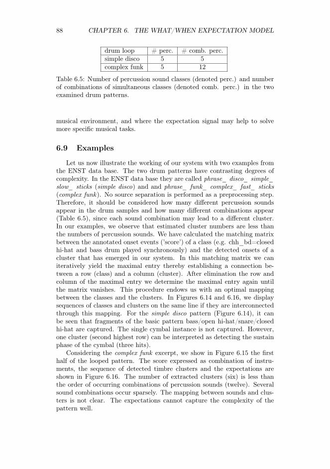
88 CHAPTER 6. THE WHAT/WHEN EXPECTATION MODEL
drum loop # perc. # comb. perc.simple disco 5 5complex funk 5 12
Table 6.5: Number of percussion sound classes (denoted perc.) and numberof combinations of simultaneous classes (denoted comb. perc.) in the twoexamined drum patterns.
musical environment, and where the expectation signal may help to solvemore specific musical tasks.
6.9 Examples
Let us now illustrate the working of our system with two examples fromthe ENST data base. The two drum patterns have contrasting degrees ofcomplexity. In the ENST data base they are called phrase_ disco_ simple_slow_ sticks (simple disco) and and phrase_ funk_ complex_ fast_ sticks(complex funk). No source separation is performed as a preprocessing step.Therefore, it should be considered how many different percussion soundsappear in the drum samples and how many different combinations appear(Table 6.5), since each sound combination may lead to a different cluster.In our examples, we observe that estimated cluster numbers are less thanthe numbers of percussion sounds. We have calculated the matching matrixbetween the annotated onset events (’score’) of a class (e.g. chh_bd=closedhi-hat and bass drum played synchronously) and the detected onsets of acluster that has emerged in our system. In this matching matrix we caniteratively yield the maximal entry thereby establishing a connection be-tween a row (class) and a column (cluster). After elimination the row andcolumn of the maximal entry we determine the maximal entry again untilthe matrix vanishes. This procedure endows us with an optimal mappingbetween the classes and the clusters. In Figures 6.14 and 6.16, we displaysequences of classes and clusters on the same line if they are interconnectedthrough this mapping. For the simple disco pattern (Figure 6.14), it canbe seen that fragments of the basic pattern bass/open hi-hat/snare/closedhi-hat are captured. The single cymbal instance is not captured. However,one cluster (second highest row) can be interpreted as detecting the sustainphase of the cymbal (three hits).
Considering the complex funk excerpt, we show in Figure 6.15 the firsthalf of the looped pattern. The score expressed as combination of instru-ments, the sequence of detected timbre clusters and the expectations areshown in Figure 6.16. The number of extracted clusters (six) is less thanthe order of occurring combinations of percussion sounds (twelve). Severalsound combinations occur sparsely. The mapping between sounds and clus-ters is not clear. The expectations cannot capture the complexity of thepattern well.

6.9. EXAMPLES 89
-4 -2 0 2 4
First Component-3
-2
-1
0
1
2
3
4
5
Seco
nd C
om
ponent
Figure 6.13: Acoustic properties of the detected attacks, plotted along their2 first principal components. Colors and shapes indicate timbre clustersassignments.
0 2 4 6 8 10 12
bd
sd
chh
ohh
cr1 x
x
x
x
x
x
x
x
x
x
x
x
x
x
x
x
x
x
x
x
x
x
x
x
x
x
x
x
x
x x
x
x
x
x
x
x
x
x
x
x x
x
x
x
x
x
x x
x
x
x
x
x
x x
Simple Disco: Score
Per
cuss
ion
So
un
ds
0 2 4 6 8 10 12bd_chh
bd_chh_sdchhohh
bd_cr1 x
x
x
x
x
x
x
x
x
x
x
x
x
x
x
x
x
x
x
x
x
x
x
x
x
x
x
x
x
x
x
x
Detection / Expectation on Sound Combinations
o
o o o
o
o
o
o
o
o
o
o
o
o
o
o
o
o
o
o
o
o
o
o
o
o
o
o
o
o
o
o
>
>
> >
>
> > >
>
>
>
>
>
>
>
>
>
>
>
>
>
>
>
>
>
>
>
>
>
>
>
>
Time (s)
Figure 6.14: Top: score of the simple disco excerpt. Bottom: Score repre-sented as combinations of instruments (’x’) , extracted cluster sequence (’o’)and expected events (’>’) according to the independent scheme (bottom) forthis excerpt. This acoustic pattern is learned well after processing the first8 s of signal.

90 CHAPTER 6. THE WHAT/WHEN EXPECTATION MODEL
0 1 2 3 4 5 6 7
bd
sd
chh
ohh
cr1
x
x
x
x
x
x
x x
x
x
x
x
x
x
x
x
x
x
x
x
x
x
x
x
x x
x
x
x
x
x
x
x
xxx x
x
x
x
x
xx
x
x
x
x
x
x
x
x
x
xxx
x
x
x
x
x
x
x
x
x
x
x
x
x
x x
x
x
x
x
x
x
x
x
x
Complex Funk: Score
Per
cuss
ion
So
un
ds
Figure 6.15: Score of the complex funk excerpt.
0 2 4 6
bd
bd_chh
sd
bd_sd
bd_chh_sd
chh_sd
chh
ohh
ohh_sd
bd_ohh
bd_chh_cr1
bd_cr1
x
x
x
x
x
x
x
x
x
x
x
x
x
x
x
x
x
x
x
x
x
x
x
x
xx x
x
x
x
x
x
x
x
x
x
x
x
xx
x
x
x
x
x
x
x
x
x
x
x
xx
x
x
Complex Funk
o
o o o o
o
o
o
o
oo
o
o
oo
o
o
o
o
o o
o
o
o
oo
o
o
o
o
o
oo
o o
o
o
o
o
o
o
oo
oo
>
> >
> > >
>
> >
>>> >>
>
> >>
>
>>
> >
>
> >
>>
>
>
>
>>
>>
>
>
>
>
>
>
>
>
>
>
Time (s)
Per
cuss
ion
So
un
ds
Figure 6.16: Score represented as combinations of instruments (’x’) , ex-tracted cluster sequence (’o’) and expected events (’>’) according to theindependent scheme (bottom) for the complex funk excerpt. The systemfails in representing adequately this irregular excerpt and cannot generateuseful expectations.

CHAPTER 7Integration in MusicProcessing Systems
7.1 Chapter Summary
The model presented with this thesis has been integrated in differentmusical systems, each one highlighting specific aspects of it. The represen-tation layer has been integrated into a real-time music transcription system.The combination of representation and expectation modules has been thebasis of a software tool able to visualize and evaluate the ongoing represen-tation expectation of an attended signal, which was developed within theEmcap project 1. Also, this tool allows the sonification of the expectationprocess, that is, the generation of an audio rendition of the expected eventsby means of concatenative synthesis, in a fully unsupervised setting. Sonifi-cation provides a way of inspecting the internal dynamics of the what/whenexpectation model. Finally, a real-time application has been designed toprovide a real-time visualization of the system expectations.
7.2 Integration of the Representation Layer
7.2.1 A library for high-level audio description
Various aspects of the representation layer described in this thesis havebeen implemented in a C++ library called Billaboop 2. More generally,Billaboop is a library which provides high-level interaction with audio, andwas designed to be included in real-time audio applications. On the onehand, Billaboop is similar to the Aubio 3 library because it is intended to be alow-latency library for causal and possibly real-time processing. On the other
1. http://emcap.iua.upf.es/2. http://billaboop.com/lib3. http://aubio.org
91

92 CHAPTER 7. INTEGRATION IN MUSIC PROCESSING SYSTEMS
hand, Billaboop takes advantage of of a more structured and object-orienteddesign in C++, which makes it similar to the libraries CLAM 4, Marsyas 5,or Essentia 6. Moreover, Billaboop aims at integrating audio analysis, datamodelling and machine learning tools in a single library.
First, the library provides a common framework for computing audiodescriptors either in the temporal or the spectral domain. Each low level de-scriptor processing class is derived from the abstract Descriptor class. Thismakes it easy to add new descriptors to the applications, and to add new de-scriptors to the library analysis processing queue. The low-level descriptorsavailable so far are listed below:
– Zero Crossing rate– Complex Domain Detection– High Frequency Content– Spectral Centroid– Spectral Slope Regression– Energies in Bark, Gammatone, and Mel filterbanks– Mel-frequency Cepstrum CoefficientsThe library also provides a set of mathematical and statistical tools that
enable to derive new descriptors from the base set. These tools includemethods such as linear regression, data normalization or peak picking. Thisenables to easily build higher-level descriptors such as temporal regressionover the instantaneous energy of a given filterbank or onset detectors. Higherlevel descriptors, resulting for a categorization process, can be extracted withthe following machine learning algorithms.
– K-Nearest Neighbours– Support Vector Machines (SVM, using a wrapper to the libsvm 7 li-
brary)– K-means clustering– Online K-MeansThe supervised algorithms can be run in testing mode based on previously
built models. However, it is also possible to train models from the library,which is useful from running validation experiments or to provide embeddedlearning in applications that use the library.
The Billaboop library thus provides supervised or unsupervised detectionof acoustic events based on arbitrary descriptors. The resulting higher-leveldescription of the incoming audio stream enables to perform the followingtasks:
– Query by audio similarity– Query by cluster prototype– Concatenative synthesisBillaboop is available under the GNU general Public License (GNUGPL).
It has been tested on Windows, MacOSX and Linux environments. In thenext section we present a front-end to the transcription layer provided bythis library.
4. http://clam-project.org5. http://marsyas.sness.net6. http://mtg.upf.edu/technologies/essentia7. http://www.csie.ntu.edu.tw/~cjlin/libsvm
7.3. ANALYZING, EVALUATING AND SONIFIYING 93
7.2.2 Real-time interaction front-end
A real-time application called Billaboop Drums has been implemented toprovide a virtual drumming interface. The main idea is to provide to usersa real-time transcription of percussive strokes detected in the signal input.The user can choose to use a predefined transcription model or to build onewithin the application. This makes it possible to use arbitrary sounds (tooldrumming, hand clapping, beat boxing) to control the application. As aresult, the application returns either a MIDI transcription of the performedrhythm or can control an internal sampler by performing query by similarity.
A screenshot of the Billaboop Drums VST plug-in is shown in Figure 7.1.The vertical slider controls the onset detection sensitivity. Three targetclasses are defined, namely Bass Drum, Snare Drum and Hi Hat. The radiobuttons auto, wizard, and edit enable to choose the sound detection recog-nition mode. When running the auto recognition mode the programs uses apreviously built, general purpose sound classification model. As reported in(Hazan, 2005b), this model has been trained on a dataset using sources fromprofessional and amateur beatboxers, as well as arbitrary sounds (e.g. keys,spoon hitting a tea mug, handclaps). The accuracy of this model has beendiscussed in (Hazan, 2005b), and showed that a cross-validation accuracy of81% can be attained if the system has to return a decision in 11ms. Thismakes this general model usable for real-time performance especially becausehigher detection rates can be attained when a given user gets used to thepredefined model. However, in other cases it is preferable to allow the userto build its own recognition model. This can be achieved on-line, using theedit or wizard mode. In this case, the user provides a number of exemplaracoustic strokes for each drum label. Then, the embedded learning compo-nent provided by the Billaboop library enables to train a recognition model.The wizard mode makes it faster to provide exemplar strokes by guiding theuser with spoken instructions without the need of using the graphical userinterface.
7.3 Analyzing, evaluating, and sonifiyingrepresentation and expectation
We present in this section the command line tool used to perform ex-pectation generation experiments using the what/when expectation modelpresented in this thesis. This tool is called Billabio, and was first introducedin (Hazan et al., 2007). Billabio is implemented in the Python 8 program-ming language using the Numpy package 9. The resource-intensive opera-tions such as audio analysis are handled by two external libraries, namelyAubio and Billaboop. The general system block diagram has been presentedin Figure 6.1. Additionally, detailed diagrams specific to a given expectationscheme have been shown in Figure 6.5 and 6.6.
8. http://python.org9. http://numpy.scipy.org

94 CHAPTER 7. INTEGRATION IN MUSIC PROCESSING SYSTEMS
Figure 7.1: Screenshot of the Billaboop Drums VST plug-in.
The general idea behind this tool is to study the dynamics of the what/whenexpectation system by providing visualization, evaluation and sonification ofthe expectation process. The audio analysis stage corresponding to featureextraction can be parametrized, allowing to choose from a set of descriptors.The visualization module has been used to produce all the figures presentedin previous chapter. The evaluation can be performed either in an unsuper-vised or supervised settings. In the latter case, annotated files correspondingto each of the analyzed audio files need to be provided. The behaviour ofthe system modules can be configured. We show in Table 7.1 the list ofcommand-line parameters that can be passed to the application. We reportthe main parameters that can be controlled. First, the user launches theanalysis process by providing an audio file playlist. Indeed, because we use adynamic listening model, the ordering of the audio sources is important. Thenumber of repetitions can be provided. Then, the auditory front end can beconfigured by choosing the onset detection thresholds and technique used,the list of descriptors to use and the descriptors averaging technique, if any.The dimensionality reduction module can be controlled by tuning the PCAprocess and the online K-means clustering parameters. Finally, the expec-tation module can be configured: the maximum context size to consideredby the PPM expectators and the expectation scheme can be chosen.

7.3. ANALYZING, EVALUATING AND SONIFIYING 95
Usage: ./billabio [options] soundfile [soundfile_2 soundfile_N]
Options:-h, --help show this help message and exit-B BUFSIZE, --bufsize=BUFSIZE
buffer size [default=1024]-H HOPSIZE, --hopsize=HOPSIZE
overlap size [default=512]-g NGRAMSIZE, --cngramsize=NGRAMSIZE
the size of the n-grams [default=5]-s EXPECTATORSCHEME, --expscheme=EXPECTATORSCHEME
the expecator scheme [default=indep]-t DETECTIONTHRESHOLD, --threshold=DETECTIONTHRESHOLD
onset detection threshold [default=0.5]-p DOPLOT, --plot=DOPLOT
whether to plot the results on a separate window(file/window/no) [default=no]
-S, --sonify whether to sonify the transcription and theexpectation
-r NREPEATS, --repeat=NREPEATShow many times to repeat the input sound [default=1]
-d DESCMODE, --descmode=DESCMODEwhether to store each descriptors on the onset frameor to compute the median the IOI region(onset/ioi/onset2) [default=ioi]
-D DESCLIST, --desclist=DESCLISTwhich timbre descriptors we aim to use. The format is"desc1 desc2", where the descriptors have to be chosenfrom the keywords: sc, zcr, pitch, mfcc [default "zcrsc pitch"]
-i INFOCRITERION, --infocriterion=INFOCRITERIONModel selection criterion (bic/aicc) [default aicc]
-e IOILRATE, --ioilrate=IOILRATEioi online k-means learning rate [default .3]
-f TIMBRELRATE, --timbrelrate=TIMBRELRATEtimbre online k-means learning rate [default .3]
-X, --pca whether to do PCA on timbre descriptors [default no]-E, --eval whether to evaluate attended excerpt against ground
truth, for each loop-P DBPATH, --dbpath=DBPATH
Database path, used for evaluation
Table 7.1: List of configurable parameters in the Billabio application
7.3.1 Implementation
The components of Billabio are written in the Python programming lan-guage, which the exception of the audio analysis processes, which are im-plemented in C. Both dimensionality reduction and next event predictionmodules, constituting the machine learning algorithms, are implemented us-ing numpy. Additionally, we use the em package 10 (Cournapeau, 2006) for
10. http://www.ar.media.kyoto-u.ac.jp/members/david/softwares/em

96 CHAPTER 7. INTEGRATION IN MUSIC PROCESSING SYSTEMS
applying the Expectation Maximization Algorithm, and the mdp package 11
(Berkes and Zito, 2007) for performing the Principal Component Analysis.
7.3.2 Sonification
Additionally, the system enables to sonify the transcription and expec-tation processes, as explained below. Expectation sonification provides asimple but powerful tool for evaluating qualitatively the system dynamicsfor encoding an audio input and generating an expectation signal. Basi-cally, we design a system, inspired by Schwarz (2004), Collins (2004) andJehan (2005) based on data-driven concatenative synthesis, as explained be-low. During the listening process, each inter-onset region is described usingsome features (e.g. Zero Crossing Rate, Centroid, MFCC, Pitch). The inter-onset region description is associated to a timbre cluster and the waveformcorresponding to this region is stored.
Consequently, we can resynthesize the transcription based on the ac-cumulated slices and events cluster assignments. The expectation moduleprovides a timeline corresponding to the future onset times for each timbrecluster. Based on this timeline, we retrieve, for each expected cluster, thewaveform which is prototypical for this cluster. This way, we can generatean output audio stream which sonifies both encoding and expectation pro-cesses. We include examples of expectation sonification for various audiofiles, either containing pitched or percussive sounds, in Appendix B.
7.4 Real-Time What/When Expectation System
The real-time what/when expectation system(Hazan et al., 2008a) is anapplication demonstrating the real-time use of the expectation model de-veloped in Chapter 6 which illustrates the when|what prediction scheme.As noted in Section 6.8, this prediction scheme enables the processing ofa polyphonic representation of events. Because this scheme is more sen-sitive to the transcription noise than the joint and independent schemes,it requires an accurate polyphonic detection model. The online K-meansalgorithm we introduced in previous chapter cannot model the occurrenceof simultaneous strokes for different categories, for this reason we providehere a supervised detection model that can handle a polyphonic representa-tion of percussive strokes. The block diagram corresponding to a supervisedpolyphonic detection model is shown in Figure 6.12. The representation ofacoustic units relies on a set of supervised classifiers that were trained on theMAMI database (Tanghe et al., 2005b), which consists of annotated drumsamples in a polyphonic context. Our implementation allows the use of ar-bitrary binary libsvm models for each sound detector. Here we have trainedfour binary classifiers to detect the occurrence of the following labels: BassDrum, Snare Drum, Open Hat, and Closed Hat. The binary classifiers areSVM models trained using the libsvm wrapper that is included in the Bill-aboop library.
11. http://mdp-toolkit.sourceforge.net

7.4. REAL-TIME WHAT/WHEN EXPECTATION SYSTEM 97
Figure 7.2: Screenshot of the real-time what/when expectation system, ana-lyzing the song Highway to Hell (AC/DC, 1979). Four stroke categories areused, and correspond to four rows and colors.
Salient events in the incoming music stream are detected and categorized.For each timbre category, expectation of the future events to be heard is com-puted. The analysis, sonification, and the visualization of transcription andexpectation are done real-time, which enables an interactive user experience.The visualization of musical events is divided into two parts: past (left) andfuture (right). The vertical red line indicates the present. At each instant,when a perceptual hit is detected, a point appears at the present. Detectedevents of each category trigger a specific drum sample, in a way similar tothe Billaboop Drums implementation. The color and row correspond to aspecific timbre category. Detected stokes appear as solid colored balls, inthe present line and they scroll to the left as the acoustic stream is analyzed.Based on the detected events, expectations are generated. Empty circlescorresponding to those expectations are consequently displayed as futureevents, at the right of the present line. When a detected event matches andexpected event, this means that the expectation is fulfilled.
We show a screenshot of the system while processing a commercial record-ing in Figure 7.2. The recording used for this example is Highway to Hell(AC/DC, 1979). The detected and expected events correspond from to tobottom, to the Bass Drum, Snare Drum, Open Hat and Closed Hat detectionmodels. We can see the expectation pattern displayed with empty circles.Some expectations, namely in the Bass Drum, Snare Drum and Closed Hatcategories are matched. Also, we can notice in the top left corner a an un-matched expectation for the Bass Drum, that corresponds to an event thatwas missed by the detection model but was expected by the system, becauseit was following the regularities of the Bass Drum pattern analyzed so far.

98 CHAPTER 7. INTEGRATION IN MUSIC PROCESSING SYSTEMS
7.5 Concluding remarks
In this dissertation we have stressed the interplay that takes place be-tween representation, learning, and expectation. We have introduced inthis chapter different implementations that enable the comparison of designalternatives, and proposed a musical system that allows the use of repre-sentation and expectation models for processing spectro-temporal events inmusical audio signals. Of course, the representation we use does not allowus to process some important events in music such as chords or harmony,and by no means we claim to have proposed a system that can process allkind of musical signals. As such, these tools and applications have to beseen as a starting point for making representation and expectation modelsavailable for processing musical audio, and are aimed to evolve into novelapplication uses for research, compositional and interaction purposes. Inthe next chapter, we summarize and discuss the whole approach presentedin this dissertation, and present general conclusions.

CHAPTER 8Conclusions and future
work directions
In this dissertation, we have shown that it is possible to build a mu-sic representation and expectation model that exhibits basic characteristicsfound in auditory perception and cognitive systems:
– Causal processing: new acoustic information is processed as it becomesavailable.
– Adaptation: Incoming information enables the refinement of the inter-nal representation of musical sequences.
– Prediction: The sensory information and current representation of theacoustic stream enables the formation of expectations regarding forth-coming events.
These principles have formed the basic thread from which we have pre-sented and discussed the following contributions.
8.1 Contributions
A prediction-based account of implicit learning We have proposed inChapter 4 an approach to modelling the acquisition of statistical regularitiesin tone sequences. We have used two Artificial Neural Network architecturesto simulate the general learning trend observed by Saffran et al. (1999). Ourresults show that the choice of the network architecture has little effect on thepost-exposure accuracy, which suggests that an extended temporal contextis not necessary to model this task.
The simulations based on interval representations such as Pitch ClassInterval or Contour did not consistently account for the experimental results.However, using a tone sequence encoding based on Pitch Class, we observed,for all experiments and languages, an increase of the categorization accuracyof words versus non-words and words versus part-words in a population of
99

100 CHAPTER 8. CONCLUSIONS
prediction models after they have been exposed to tone sequences containingstatistical regularities.
In this learning modelling experiment, our main contribution is two-fold.First, we showed that the choice of the representation of the musical eventsmust be taken into account when modelling music perception in humans andmachines, even when working in the symbolic domain. Furthermore, our re-sults suggest that the common assumption that pitch sequences are encodedas abstract interval values cannot be taken for granted. More importantly,we have proposed a framework for simulating and evaluating the outcome ofsequence learning experiments based on the forced-choice task paradigm ina way that allows for the comparison of arbitrary learning algorithms. Thisframework is extensible and enables the assessment of whether learning ar-chitectures can simulate further empirical findings using real-world musicalsequences (Schellenberg, 1996; Dalla Bella et al., 2003).
What/When expectation model We have presented an unsupervisedand causal approach to transcribe, encode and generate what and whenexpectations based on constant-tempo musical audio, using both timbre andtiming dimensions. Our system analyzes and represents events based onbeats and onset, and creates a set of categories, in either an unsupervisedor supervised way to describe incoming events. Then, the model learns theregularities of the incoming signal to create expectations. As such, this canbe considered as a mid-level approach to expectation modelling applied toaudio, if we compare it to systems that focus on auditory sequences (Brown,1993; Cooke, 1993; Ellis, 1996), information-theoretic approaches that do notexplicitly extract semantic information from the musical audio (Abdallah,2002; Dubnov, 2006; Cont, 2008), and models that focus on symbolic orMIDI representations of music (Bharucha and Todd, 1989; Todd and Loy,1991; Mozer, 1994; Tillmann et al., 2000; Lartillot et al., 2001; Pachet, 2003;Eck and Schmidhuber, 2002; Pearce and Wiggins, 2004).
Alternatives to combining the what and when dimensions have been pre-sented and evaluated. We have illustrated the steps involved in the fea-ture extraction, dimensionality reduction, learning and expectation processesand we have compared these steps quantitatively using a corpus of percus-sive excerpts. Three expectation schemes, namely independent, joint, andwhen|what schemes were defined to take into account alternative viewpointsregarding how musical events are organized. From a cognitive perspectivethose schemes may be associated to distinct processing pathways of the mu-sical stream (Peretz and Zatorre, 2005).
A set of statistics has been presented to characterize the system learn-ing abilities. An evaluation of the system components has been performed.The results show that, on the one hand, the system’s ability to produce anexpectation timeline that agrees with ground truth annotations depends onthe quality of the transcription process, and that the performance of thewhen|what scheme is more severely degraded when the transcription accu-racy degrades. On the other hand, even if the representation of the systemdoes not accurately fit the ground truth, our results suggested that the sys-

8.2. OPEN ISSUES 101
tem is able to use and maintain an internal representation of the musicalstream to identify patterns whose regularities can be learned. In this lat-ter case, the transcription step may be seen as a musically-informed sparserepresentation process. Therefore, we suggest that the model may be evalu-ated according to the usefulness and robustness of its representation ratherthan using ground truth annotations. Besides, we have suggested that theexpectation signal may describe the structure of musical patterns in a causalmanner and have shown the expectation entropy measure could provide in-formation about the structure of musical streams. This expectation-basedsignals may provide an alternative approach to perform structural segmen-tation tasks.
Integrating representation and expectation models into musicalsystems By their nature, causal systems accommodate with the time dy-namics of the sensory data they process. In the case of audio, real-timesystems can be implemented to provide a seamless interaction with users,and enables novel uses for musical or educational purposes, as well as en-tertainment. Among the possible applications of this work are: musicallearning applications that do not require a specific hardware such as a key-board, accompaniment applications, or audio-driven games. Here, our mainmotivation is to demonstrate that even if there is room for improvement inalmost all components of the system, it is already possible to design novelinteractive settings and applications that take advantage of representing andcreating expectations from audio signals. Because musicians and enthusiastsare among the most valuable users of the technologies that may derive fromthis research, they should be given ways to access and understand those tech-nologies. This way, users may help to both broaden and refine the spectrumof possible systems that enable a meaningful musical interaction.
8.2 Open issues
In spite of the contributions and achievements presented here, we wouldlike to see this research as starting point which highlights interesting issuesin the field of expectation modelling. Here we attempt to describe the mostrelevant issues and work directions to this work.
8.2.1 Measuring mismatch with the environment
One objection that can be made concerning the approach proposed hereis that it creates and maintains a representation of the musical events, gener-ates expectations based on this, but does not retrospectively compare theseexpectations with actual events to refine its representation. This would cor-respond to Ellis’ reconciliation process (Ellis, 1996) or the appraisal stepin the theory developed by Huron (2006). To this extent, even though oursystem can create symbolic expectations that can be mapped into absolutetime by the representation layer, there is no further feedback processing norreuse of the expectation mismatch with the environment. It is worth noting

102 CHAPTER 8. CONCLUSIONS
that our architecture could handle this additional processing, but we needto properly define mismatch measurements to track which expectations arefulfilled, and how they are fulfilled. Some starting points to this would be thedistances measures proposed by Paiement (2008), as well as works focusingon audio similarity (Pampalk et al., 2008).
8.2.2 Scales of music processing
Another outstanding issue in our research is the need to address thevarious temporal scales involved in music processing and learning.
Representation over multiple time scales In our model, we have fo-cused in representing musical structure in terms of relations between eventonsets over several acoustic dimensions. While being simple enough to becomputationally tractable and rich enough to describe several aspects of mu-sical sequences at the same time, this time scale may be inaccurate to modelmore precise acoustic inflections that could contain relevant information.Conversely, if we aim consider a musical excerpt from a broader viewpoint,we might need to use a longer time scale. It is worth noting that, by creatingan expectation signal between event onsets (that can be considered in thetimescale of a note), the system may able to implicitly perform segmenta-tion on a bar timescale, as the expectation entropy patterns suggest (seeSection 6.7.7). As a future work, it may be possible to represent and learnthe regularities of the expectation entropy patterns.
Learning timescale In the majority of the experiments presented here,we have repeatedly presented to the system short music excerpts and assessedwhether the system was able to follow those excerpts through repetitions.However, because the model’s running state proceeds in a causal way, ourimplementation could virtually analyze musical streams of arbitrary dura-tion. Consequently, we need to investigate how to assess longer-term effectsof learning, what musical memory contents are maintained and how they aremaintained through the exposure to successive and possibly distinct musicalsequences. For instance, we would like to assess to which extent our modelcan keep some information about previous excerpts when heading at theend of a playlist. One actual limitation to progress in that direction is thatour model performs the bootstrap estimation only at the beginning of anyexposure. Alternative strategies should be investigated, such as performingbootstrap when a new representation is needed, or continuously performingthe bootstrap step in parallel to the running state.
8.2.3 Towards an account of auditory learningexperiments using the what/when model
In Chapter 4 we have proposed a framework to modelling the acquisitionof statistical regularities in tone sequences, represented in a symbolic form.Then, in Chapter 6, we have introduced an expectation model that learns torepresent auditory events in a meaningful way. From these two contributions,

8.3. A PERSONAL CONCLUDING NOTE 103
it seems natural to investigate whether the what/when expectation modelcan provide an account of empirical results dealing with auditory learningexperiments that focus on the interaction between acoustical cues and timestructures (Newport and Aslin, 2004; Tillmann and McAdams, 2004), butthis would be better included in the research agenda of music cognitionscientists.
8.3 A personal concluding note
This dissertation is in essence a multidisciplinary account to model mu-sic expectation from areas such as auditory perception, learning, expectationmodelling, and information theory. As such, an important part of my re-search has consisted in building bridges across these disciplines, and tryingto view issues that were specific of a given area from a distinct viewpoint.Firstly, this dissertation aims to provide tools to cognitive science and se-quence learning researchers to address computationally real-world auditoryand musical stimuli. Likewise, it aims at enabling MIR and auditory per-ception researchers to investigate the effects of learning and the usefulnessof an ever-evolving representation of the musical signal. Finally, I hope thatthe contributions presented here can serve as a basis for designing an inter-active music system driven by cognitive principles, pattern recognition andpredictive learning.


Bibliography
Abdallah, S. (2008). A critique of dubnov’s "Information Rate". TechnicalReport C4DM-TR08-11, Center for Digital Music, Queen Mary, Universityof London.
Abdallah, S. and Plumbley, M. (2009). Information dynamics: patterns ofexpectation and surprise in the perception of music. Connection Science,21(2):89–117.
Abdallah, S. A. (2002). Towards Music Perception by Redundancy Reductionand Unsupervised Learning in Probabilistic Models. PhD thesis, KingśCollege London, London, UK.
Akaike, H. (1974). A new look at the statistical model identification. Auto-matic Control, IEEE Transactions on, 19:716–723.
Allan, L. (1979). The perception of time. Perception and Psychophysics,26:340–354.
Allauzen, C., Crochemore, M., and Raffinot, M. (1999). Factor oracle: Anew structure for pattern matching. In Proceedings of the 26th Conferenceon Current Trends in Theory and Practice of Informatics on Theory andPractice of Informatics, pages 295 – 310.
Altmann, G. T. M., Dienes, Z., and Goode, A. (1995). Modality indepen-dence of implicitly learned grammatical knowledge. Journal of Experi-mental Psychology-Learning Memory and Cognition, 21(4):899–912.
Assayag, G., Bloch, G., and Chemillier, M. (2006). «OMax-Ofon». In Pro-ceedings of Sound and Music Computing (SMC), Marseille, France.
Assayag, G. and Dubnov, S. (2004). Using Factor Oracles for machine Im-provisation. Soft Computing, 8(9):604–610.
Aucouturier, J. J. and Sandler, M. (2001). Segmentation of musical signalsusing hidden markov models. Preprints Audio Engineering Society.
Barlow, H. (2001). The exploitation of regularities in the environment bythe brain. Behavioral and Brain Sciences, 24:602–607.
Berkes, P. and Zito, T. (2007). Modular toolkit for data processing (version2.1).
105

106 BIBLIOGRAPHY
Bharucha, J. J. and Todd, P. M. (1989). Modeling the perception of tonalstructure with neural nets. Computer Music Journal, 13:44–53.
Bigand, E., Perruchet, P., and Boyer, M. (1998a). Implicit learning of anartificial grammar of musical timbres. Cahiers de psychologie cognitive,17(3):577–600.
Bigand, E., Perruchet, P., and Boyer, M. (1998b). Implicit learning of anartificial grammar of musical timbres. Cahiers de psychologie cognitive,17(3):577–600.
Biles, J. (1994). Genjam: A genetic algorithm for generating jazz solos. InProceedings of the International Computer Music Conference.
Bishop, C. M. (1995). Neural Networks for Pattern Recognition. ClarendonPress, Oxford.
Boltz, M. G. (1993). The generation of temporal and melodic expectanciesduring musical listening. Perception and Psychophysics, 53:585–585.
Bottou, L. (2004). Stochastic learning. Advanced Lectures On MachineLearning: ML Summer Schools 2003, Canberra, Australia, February 2-14,2003, Tübingen, Germany, August 4-16, 2003: Revised Lectures.
Botvinick, M. M. and Plaut, D. C. (2006). Short-term memory for serial or-der: A recurrent neural network model. Psychological Review, 113(2):201–233.
Box, G. E. P., Jenkins, G. M., and Reinsel, G. C. (1976). Time seriesanalysis: forecasting and control. Holden-day San Francisco.
Bregman, A. S. (1990). Auditory Scene Analysis. MIT Press, Cambridge,MA.
Brossier, P. (2006). Automatic Annotation of Musical Audio for InteractiveApplications. PhD thesis, Centre for Digital Music, Queen Mary Univer-sity of London, London, UK.
Brossier, P., Bello, J., and Plumbley, M. (2004). Fast labelling of notes inmusic signals. In Proceedings of the 5th International Symposium on MusicInformation Retrieval (ISMIR 2004), pages 331–336, Barcelona, Spain.
Brown, G. J. (1993). Computational auditory scene analysis: A represen-tational approach. The Journal of the Acoustical Society of America,94(4):2454.
Burton, A. R. and Vladimirova, T. (1999). Generation of musical sequenceswith genetic techniques. Computer Music Journal, 23(4):59–73.
Caclin, A., Brattico, E., Tervaniemi, M., Näätänen, R., Morlet, D., Giard,M., and McAdams, S. (2006). Separate neural processing of timbre di-mensions in auditory sensory memory. Journal of Cognitive Neuroscience,18(12):1959–1972.

BIBLIOGRAPHY 107
Cano, P. (2006). Content-Based Audio Search: From Fingerprinting ToSemantic Audio Retrieval. PhD thesis, Universitat Pompeu Fabra.
Carpinteiro, O. (2000). A hierarchical self-organising map model for sequencerecognition. Pattern Analysis and Applications, 3:279–287.
Casey, M. (2002). General sound classification and similarity in MPEG-7.Organised Sound, 6(02):153–164.
Cemgil, A. T., Kappen, H. J., Dietterich, T. G., and Becker, S. (2002).Tempo tracking and rhythm quantization by sequential monte carlo. InDietterich, Th. G.; Becker, S.; Ghahramani, Z.(eds.), Advances in neuralinformation processing systems 14: proceedings of the 2002 conference,page 1361. Cambridge, Mass.; London, England: MIT Press.
Clarke, E. (1989). The perception of expressive timing in music. Psycholog-ical Research, 51:2–9.
Clarke, E. F. (1987). Levels of structure in the organization of musical time.Contemporary music review, 2(1):211–238.
Cleary, J. G. and Witten, I. H. (1984). A comparison of enumerative andadaptive codes. IEEE Transactions on Information Theory, 30(2):306–315.
Cleeremans, A. (1993). Mechanisms of implicit learning: Connectionist mod-els of sequence processing. MIT press, Cambridge, MA.
Cleeremans, A. and McClelland, J. (1991). Learning the structure of eventsequences. Journal of Experimental Psychology: General, 120(3):235–253.
Collins, N. (2004). On onsets on-the-fly: Real-time events segmentation andcategorization as a compositional effect. In Proceedings of the First Soundand Music Computing Conference (SMC’04), Paris, France.
Conklin, D. and Anagnostopoulou, C. (2001). Representation and discov-ery of multiple viewpoint patterns. In Proceedings of the InternationalComputer Music Conference, pages 479–485, La Havana, Cuba.
Cont, A. (2008). Modeling Musical Anticipation: From the time of musicto the music of time. PhD thesis, University of Paris 6 and University ofCalifornia in San Diego.
Cooke, M. (1993). Modelling auditory processing and organisation. Cam-bridge University Press, Cambridge, UK.
Cooper, G. and Meyer, L. (1960). The rhythmic structure of music. Univer-sity of Chicago Press, Chicago, IL.
Cournapeau, D. (2006). Pyem, a python package for gaussian mixture mod-els. Technical report, University of Kyoto, Graduate School of Informatics.
108 BIBLIOGRAPHY
Creel, S. C., Newport, E. L., and Aslin, R. N. (2004). Distant melodies: Sta-tistical learning of nonadjacent dependencies in tone sequences. Learning,Memory, 30:1119–1130.
Dalla Bella, S., Peretz, I., and Aronoff, N. (2003). Time course of melodyrecognition: a gating paradigm study. Perception and Psychophysics,65(7).
Davies, M. E. P., Brossier, P. M., and Plumbley, M. D. (2005). Beat trackingtowards automatic musical accompaniment. In Proceedings of the 118thAES convention, Barcelona, Spain.
Davies, M. E. P. and Plumbley, M. D. (2005). Beat tracking with a two statemodel. In Proceedings of the IEEE International Conference on Acoustics,Speech, and Signal Processing (ICASSP ’05), pages 241–244, Philadelphia,Penn., USA.
Davis, S. and Mermelstein, P. (1980). Comparison of parametric representa-tions for monosyllabic word recognition in continuously spoken sentences.Pattern Recognition and Artificial Intelligence, RCH Chen, ed., AcademicPress: New York, 28(4):357–366.
Demany, L., McKenzie, B., and Vurpillot, E. (1977). Rhythm perception inearly infancy. Nature, 266:718–719.
Dempster, A., Laird, N., and Rubin, D. (1977). Maximum likelihood fromincomplete data via the EM algorithm. Proceedings of the Royal StatisticalSociety, B-39:1–38.
Desain, P. and Honing, H. (2003). The formation of rhythmic categories andmetric priming. Perception, 32:341–365.
Dixon, S. (1997). Beat Induction and Rhythm Recognition. In Proceedings ofthe 10th Australian Joint Conference on Artificial Intelligence: AdvancedTopics in Artificial Intelligence, page 320. Springer-Verlag.
Downie, J. S. (2003). Music information retrieval. Annual Review of Infor-mation Science and Technology, 37(1):295–340.
Drake, C. (1998). Psychological processes involved in the temporal organi-zation of complex auditory sequences: universal and acquired processes.Music Percept., 16:11–26.
Dubnov, S. (2006). Spectral anticipations. Computer Music Journal,30(2):63–83.
Dubnov, S. (2008). Unified view of prediction and repetition structure in au-dio signals with application to interest point detection. IEEE Transactionson Audio, Speech, and Language Processing, 16(2):327–337.
Duxbury, C., Bello, J., Davies, M., and Sandler, M. (2003a). Complexdomain onset detection for musical signals. Proceedings Digital AudioEffects Workshop (DAFx).

BIBLIOGRAPHY 109
Duxbury, C., Bello, J. P., Davies, M., and Sandler, M. (2003b). Complexdomain onset detection for musical signals. In Proc. Digital Audio EffectsWorkshop (DAFx).
Eck, D. and Schmidhuber, J. (2002). Learning the long-term structure ofthe blues. Lecture Notes in Computer Science, Proceedings of ICANNConference, 2415:284–289.
Ellis, D. P. W. (1996). Prediction-driven Computational Auditory SceneAnalysis. PhD thesis, Massachusetts Institute of Technology, MA, USA.
Elman, J. (1990). Finding structure in time. Cognitive Science, 14(2):179–211.
Ferrand, M., Nelson, P., and Wiggins, G. (2002). A probabilistic modelfor melody segmentation. In 2nd International Conference on Music andArtificial Intelligence, University of Edinburgh, UK.
Foote, J. (1999). Visualizing music and audio using self-similarity. In Pro-ceedings of the seventh ACM international conference on Multimedia (Part1), pages 77–80. ACM New York, NY, USA.
Franklin, J. A. (2004). Recurrent neural networks and pitch representationsfor music tasks. In Barr, V. and Markov, Z., editors, Proceedings of theSeventeenth International Florida Artificial Intelligence Research SocietyConference, Miami Beach, Florida, USA. AAAI Press.
Ghezzi, C. and Mandrioli, D. (1979). Incremental parsing. ACM Transac-tions on Programming Languages and Systems (TOPLAS), 1(1):58–70.
Gillet, O. and Richard, G. (2004). Automatic transcription of drum loops.Proceedings of the IEEE International Conference on Acoustics, Speech,and Signal Processing (ICASSP ’04), 4:269–272.
Gillet, O. and Richard, G. (2006). Enst-drums: an extensive audio-visualdatabase for drum signals processing. In Proceedings of the 7th Interna-tional Symposium on Music Information Retrieval (ISMIR 2006), pages156–159.
Gómez, E. (2006). Tonal description of music audio signals. PhD thesis,Universitat Pompeu Fabra.
Goto, M. (2001). An audio-based real-time beat tracking system for musicwith or without drum-sounds. Journal of New Music Research, 30(2):159–171.
Goto, M. (2003). A chorus-section detecting method for musical audio sig-nals. In 2003 IEEE International Conference on Acoustics, Speech, andSignal Processing, 2003. Proceedings.(ICASSP’03), volume 5.
Goto, M. and Muraoka, Y. (1995). A real-time beat tracking system for audiosignals. In Proceedings of the International Computer Music Conference,pages 171–174.

110 BIBLIOGRAPHY
Gouyon, F. and Dixon, S. (2005). A review of automatic rhythm descriptionsystems. Computer Music Journal, 29(1):34–54.
Gouyon, F. and Herrera, P. (2003). A beat induction method for musicalaudio signals. In Digital media processing for multimedia interactive ser-vices: proceedings of the 4th European Workshop on Image Analysis forMultimedia Interactive Services: Queen Mary, University of London, 9-11April 2003, page 281. World Scientific Pub Co Inc.
Gouyon, F., Pachet, F., and Delerue, O. (2000). On the use of zero-crossingrate for an application of classification of percussive sounds. In Proceedingsof the COST G-6 conference on Digital Audio Effects (DAFX-00), Verona,Italy. Citeseer.
Grachten, M., Arcos, J., and López de Mantaras, R. (2006). A case basedapproach to expressivity-aware tempo transformation. Machine Learning,65(2-3):411–437.
Grey, J. M. (1977). Multidimensional perceptual scaling of musical timbres.The Journal of the Acoustical Society of America, 61:1270.
Griffith, N. and Todd, P. M. (1999). Musical Networks. Parallel DistributedPerception and Performance. The MIT Press, Cambridge, MA.
Hainsworth, S. (2006). Beat tracking and musical metre analysis. In Signalprocessing methods for music transcription, page 440. Springer-Verlag.
Hannon, E. E. and Trehub, S. E. (2005). Metrical categories in infancy andadulthood. Psychological Science, 16(1):48–55.
Hasty, C. (1997). Meter as Rhythm. Oxford University Press.
Hazan, A. (2005a). Billaboop: Real-time voice-driven drum generator. InProceedings of Audio Engineering Society, 118th Convention.
Hazan, A. (2005b). Performing expressive rhythms with billaboop voice-driven drum generator. In Proceedings of 8th Intl. Conference on DigitalAudio Effects, Madrid, Spain.
Hazan, A. (2005c). Towards automatic transcription of oral expressive per-formances. In Proceedings of the Intelligent User Interfaces Conference(IUI 2005).
Hazan, A., Brossier, P., Holonowicz, P., Herrera, P., and Purwins, H. (2007).Expectation along the beat: A use case for music expectation models.In Proceedings of International Computer Music Conference 2007, pages228–236, Copenhagen, Denmark.
Hazan, A., Brossier, P., Marxer, R., and Purwins, H. (2008a). What/whencausal expectation modelling applied to percussive audio. In The Journalof the Acoustical Society of America, volume 123, page 3800.
BIBLIOGRAPHY 111
Hazan, A., Holonowicz, P., Salselas, I., Herrera, P., Purwins, H.;Knast, A.,and Durrant, S. (2008b). Modeling the acquisition of statistical regular-ities in tone sequences. In Prceedings of the 30th Annual Meeting of theCognitive Science Society, pages 1088–1094.
Hazan, A., Marxer, R. ;Brossier, P., Purwins, H.;Herrera, P., and Serra, X.(2009). What/when causal expectation modelling applied to audio signals.Connection Science, 21:119–143.
Hazan, A., Ramirez, R., Maestre, E., Perez, A., and Pertusa, A. (2006).Modelling expressive performance: A regression tree approach based onstrongly typed genetic programming. In Proceedings of the EuropeanWorkshop on Evolutionary Music and Art, volume 3907, pages 676–672,Lausanne, Switzerland. Springer.
Hermansky, H. (1990). Perceptual linear predictive (PLP) analysis of speech.The Journal of the Acoustical Society of America, 87:1738.
Hermansky, H. and Morgan, N. (1994). RASTA processing of speech. IEEETransactions on Speech and Audio Processing, 2(4):578–589.
Herrera, P., Yeterian, A., and Gouyon, F. (2002). Automatic classification ofdrum sounds: a comparison of feature selection methods and classificationtechniques. Music and Artificial Intelligence, pages 69–80.
Hochreiter, S. and Schmidhuber, J. (1997). Long short-term memory. NeuralComputation, 9(8):1735–1780.
Homer, A. and Goldberg, D. E. (1991). Genetic algorithms and Computer-Assisted music composition. In Proceedings of the Fourth InternationalConference on Genetic Algorithms, volume 51, page 437, San Fransisco,CA. Morgan Kaufmann Publishers.
Huron, D. (2006). Sweet anticipation. MIT Press, Cambridge, MA.
Jaeger, H. (2003). Adaptive nonlinear system identification with echo statenetworks. Advances in Neural Information Processing Systems, 15:593–600.
Jayant, N. S. and Noll, P. (1984). Digital coding of waveforms. Prentice-Hall,Englewood Cliffs, NJ.
Jehan, T. (2005). Creating Music by Listening. PhD thesis, MassachusettsInstitute of Technology, MA, USA.
Jones, M. R. and Boltz, M. (1989). Dynamic attending and responses totime. Psychological Review, 96(3):459–491.
Kapur, A., Benning, M., and Tzanetakis, G. (2004). Query by beat box-ing: Music retrieval for the dj. In Proceedings of the 5th InternationalSymposium on Music Information Retrieval (ISMIR 2004).

112 BIBLIOGRAPHY
Klapuri, A. (1999). Sound onset detection by applying psychoacoustic knowl-edge. In Proceedings of the IEEE International Conference on Acoustics,Speech and Signal Processing, Phoenix, USA.
Kohonen, T. (1998). The self-organizing map. Neurocomputing, 21(1-3):1–6.
Krumhansl, C. L. (1979). The psychological representation of musical pitchin a tonal context. Cognitive Psychology, 11(3):346–74.
Krumhansl, C. L. (1989). Why is timbre so hard to understand. In Nielzén, S.and Olsson, O., editors, Structure and Perception of electroacoustic soundand music, pages 43–53. Excerpta Medica, Amsterdam.
Kuhn, G. and Dienes, Z. (2008). Learning of non local dependencies. Cog-nition, 106(1):184–206.
Lacoste, A. and Eck, D. (2007). A supervised classification algorithm for noteonset detection. EURASIP J. Appl. Signal Process., 2007(1):153–153.
Ladefoged, P. (1989). A note on Information conveyed by vowels. TheJournal of the Acoustical Society of America, 85:2223.
Large, E. W. (2000). Rhythm categorization in context. In Proceedings ofthe International Conference on Music Perception and Cognition.
Lartillot, O., Dubnov, S., Assayag, G., and Bejerano, G. (2001). Automaticmodeling of musical style. In Proceedings of the International ComputerMusic Conference (ICMC 2001), La Havana, Cuba.
Lashley, K. S. and Jeffress, L. A. (1951). Cerebral mechanisms in behavior.The problem of serial order in behavior, pages 112–136.
Lerdahl, F. and Jackendoff, R. A. (1983). A Generative Theory of TonalMusic. MIT Press, Cambridge, MA.
Lewicki, M. S. (2002). Efficient coding of natural sounds. Nat Neurosci,5(4):356–363.
London, J. (2002). Cognitive constraints on metric systems: Some observa-tions and hypotheses. Music Perception, 19(4):529–550.
London, J. (2006). How to talk about musical meter. Colloquium talks,Carleton College, MN.
Loui, P., Wessel, D., and Hudson Kam, C. (2006). Adquiring new musicalgrammars: a statistical learning approach. In Proceedings of the Interna-tional Conference on Music Perception and Cognition, Bolgna, Italy.
MacKay, D. J. C. (2003). Information Theory, Inference, and Learning Algo-rithms. Publisher: Cambridge University Press, Cambridge, UK. Availablefrom http://www.inference.phy.cam.ac.uk/mackay/itila/.
Maess, B., Koelsch, S., Gunter, T. C., and Friederici, A. D. (2001). Musicalsyntax is processed in Broca’s area: an MEG study. Nature Neuroscience.

BIBLIOGRAPHY 113
Makhoul, J. (1975). Linear prediction: A tutorial review. Proceedings of theIEEE, 63(4):561–580.
Markov, A. A. (1971). Theory of algorithms. Israel Program for ScientificTranslations.
Marxer, R., Holonowicz, P., Purwins, H., and Hazan, A. (2007). Dynamicalhierarchical self-organization of harmonic, motivic, and pitch categories.In Proceedings of the Music, Brain and Cognition Workshop, part of theNIPS conference, Vancouver, Canada.
Marxer, R., Purwins, H., and Hazan, A. (2008). An f-measure for evalua-tion of unsupervised clustering with non-determined number of clusters.Technical report, Universitat Pompeu Fabra, Music Technology Group.
Masri, P. (1996). Computer modeling of Sound for Transformation and Syn-thesis of Musical Signal. PhD thesis, University of Bristol, Bristol, U.K.
Mathews, M. V., Roberts, L. A., and Pierce, J. R. (1984). Four new scalesbased on nonsuccessive-integer-ratio chords. The Journal of the AcousticalSociety of America, 75(S1):S10.
McAdams, S. and Bregman, A. (1979). Hearing musical streams. ComputerMusic Journal, 3(4):26–60.
McAdams, S., Winsberg, S., Donnadieu, S., Soete, G., and Krimphoff, J.(1995). Perceptual scaling of synthesized musical timbres: Common di-mensions, specificities, and latent subject classes. Psychological Research,58(3):177–192.
Meyer, L. B. (1956). Emotion and meaning in music. University of ChicagoPress, Chicago, IL.
Moffat, A. (1990). Implementing the PPM data compression scheme.IEEETCOMM: IEEE Transactions on Communications, 38:1917–1921.
Mozer, M. (1994). Neural network music composition by prediction: Explor-ing the benefits of psychophysical constraints and multiscale processing.Connection Science, 6:247–280.
Narmour, E. (1990). The analysis and cognition of basic melodic structures:the Implication-Realization model. University of Chicago Press, Chicago,IL.
Narmour, E. (1992). The analysis and cognition of melodic complexity: theImplication-Realization model. University of Chicago Press, Chicago, IL.
Newport, E. L. and Aslin, R. N. (2004). Learning at a distance: I. statisticallearning of Non-Adjacent dependencies. Cognitive Psychology, 48(2):127–162.
Ong, B. S. (2006). Structural analysis and segmentation of music signals.PhD thesis, Universitat Pompeu Fabra.

114 BIBLIOGRAPHY
O’Reilly, R. C. and Munakata, Y. (2000). Computational Explorations inCognitive Neuroscience: Understanding the Mind by Simulating the Brain.MIT Press.
Pachet, F. (2003). The continuator: Musical interaction with style. Journalof New Music Research, 32(3):333–341.
Paiement, J. F. (2008). Probabilistic Models for Music. PhD thesis, EcolePolytechnique Féderale De Lausanne.
Palmer, C. (1989). Mapping musical thought to musical performance.J. of Experimental Psychology - Human Perception and Performance,15(12):331–346.
Palmer, C. and Krumhansl, C. L. (1990). Mental representations for musicalmeter. J. of Experimental Psychology - Human Perception and Perfor-mance, 16(4):728–741.
Pampalk, E., Herrera, P., and Goto, M. (2008). Computational models ofsimilarity for drum samples. IEEE Transactions on Audio Speech andLanguage Processing, 16(2):408.
Paulus, J. and Klapuri, A. (2003). Model-based event labeling in the tran-scription of percussive audio signals. In Davies, M., editor, Proceedingsof the 6th International Conference on Digital Audio Effects (DAFx-03),pages 73–77, London, UK.
Pearce, M. T. and Wiggins, G. A. (2004). Improved methods for statis-tical modelling of monophonic music. Journal of New Music Research,33(4):367–385.
Peeters, G. (2004). A large set of audio features for sound description (sim-ilarity and classification) in the CUIDADO project. CUIDADO ProjectReport.
Peeters, G., Burthe, A. L., and Rodet, X. (2002). Toward automatic musicaudio summary generation from signal analysis. In Proc. InternationalConference on Music Information Retrieval, pages 94–100. Citeseer.
Peretz, I. and Zatorre, R. (2005). Brain organization for music processing.Annual Review of Psychology, 56(1):89–114.
Povel, D. J. and Essens, P. (1985). Perception of temporal patterns. MusicPerception, 2(4):411–440.
Purwins, H., Grachten, M., Herrera, P., Hazan, A., Marxer, R., and Serra,X. (2008). Computational models of music perception and cognition II:Domain-specific music processing. Physics of Life Reviews, 5:169–182.
Ramirez, R. and Hazan, A. (2005). Understanding expressive music perfor-mance using genetic algorithms. In Proceedings of the European Workshopon Evolutionary Music and Art, pages 508–516. Springer.

BIBLIOGRAPHY 115
Reber, A. S. (1967). Implicit learning of artificial grammars. Journal ofVerbal Learning & Verbal Behavior. Vol, 6(6):855–863.
Roads, C. (2004). Microsound. MIT Press, Cambridge, MA.
Rothstein, W. (1981). Rhythm and the Theory of Structural Levels. PhDthesis, Yale University.
Rumelhart, D. and McLelland, J. (1986). Parallel Distributed Processing.MIT Press, Cambridge, MA.
Saffran, J., Johnson, E., Aslin, R., and Newport, E. (1999). Statistical learn-ing of tone sequences by human infants and adults. Cognition, 70(1):27–52.
Saffran, J. R., Newport, E. L., and Aslin, R. N. (1996). Word segmentation:the role of distributional cues. Journal of Memory and Language, 35:606–621.
Schaeffer, P. (1966). Traité des objets musicaux. Le Seuil, Paris.
Scheirer, E. D. (1998). Tempo and beat analysis of acoustic musical signals.The Journal of the Acoustical Society of America, 103:588.
Schellenberg, E. G. (1996). Expectancy in melody: Tests of the implication-realization model. Cognition, 58:75–125.
Schouten, J. F. (1968). The perception of timbre. In Reports of the 6thInternational Congress on Acoustics.
Schwarz, D. (2004). Data-Driven Concatenative Sound Synthesis. PhD the-sis, Ircam - Centre Pompidou, Paris, France.
Schwarz, G. (1978). Estimating the dimension of a model. The Annals ofStatistics, 6(2):461–464.
Smith, L. (1996). Listening to musical rhythms with progressive wavelets.In TENCON ’96. Proceedings. 1996 IEEE TENCON. Digital Signal Pro-cessing Applications, volume 2, pages 508–513 vol.2.
Snyder, B. (2000). Music and Memory: An Introduction. The MIT Press,Cambridge, MA.
Sridharan, D., Levitin, D., Chafe, C., Berger, J., and V., M. (2007). Neuraldynamics of event segmentation in music: converging evidence for disso-ciable ventral and dorsal networks. Neuron, 55(3):521–532.
Tanghe, K., Degroeve, S., and Baets, B. D. (2005a). An algorithm for de-tecting and labeling drum events in polyphonic music. In Mirex DrumRecognition Contest (part of International Symposium on Music Informa-tion Retreival).

116 BIBLIOGRAPHY
Tanghe, K., Lesaffre, M., Degroeve, S., Leman, M., Baets, B. D., andMartens, J. P. (2005b). Collecting ground truth annotations for drumdetection in polyphonic music. In Proc. 6th Int. Conf. on Music Informa-tion Retrieval (ISMIR 2005), pages 50–57.
Terhardt, E. (1998). Akustische Kommunikation. Springer, Berlin.
Tillmann, B. (2008). Music cognition: Learning, perception, expectations.In Kronland-Martinet, R., Ystad, S., and Jensen, K., editors, ComputerMusic Modeling and Retrieval. Sense of Sounds, pages 11–33. Springer,Berlin.
Tillmann, B., Bharucha, J. J., and Bigand, E. (2000). Implicit learning oftonality: A self-organizing approach. Psychological Review, 107(4):885–913.
Tillmann, B. and McAdams, S. (2004). implicit learning of musi-cal timbre sequences: statistical regularities confronted with acoustical(dis)similarities. Journal of experimental psychology, learning, memoryand cognition, 30(5):1131–1142.
Todd, P. M. and Loy, D. G. (1991). Music and Connectionism. MIT Press.
Wang, A. (2003). An industrial strength audio search algorithm. In Interna-tional Conference on Music Information Retrieval (ISMIR 2003), pages7–13.
Wang, Y., Tang, J., Ahmaniemi, A., Vaalgamaa, M., Center, N. R., andTampere, F. (2003). Parametric vector quantization for coding percussivesounds in music. In Multimedia and Expo, 2003. ICME’03. Proceedings.2003 International Conference on, volume 3.
Warren, R. and Warren, R. (1970). Auditory illusions and confusions. Sci-entific American, 223(12):30–36.
Werbos, P. (1974). Beyond Regression: New Tools for Prediction and Anal-ysis in the Behavioral Sciences. PhD thesis, Harvard University, Cam-bridge, MA.
Werbos, P. J. (1990). Backpropagation through time: what it does and howto do it. Proceedings of the IEEE, 78(10):1550–1560.
Wessel, D. L. (1979). Timbre space as a musical control structure. Computermusic journal, pages 45–52.
Williams, R. J. and Zipser, D. (1989). A learning algorithm for continuallyrunning fully recurrent neural networks. Neural computation, 1(2):270–280.
Yoshii, K., Goto, M., and Okuno, H. G. (2005). Adamast: A drum soundrecognizer based on adaptation and matching of spectrogram templates.In Mirex Drum Recognition Contest (part of International Symposium onMusic Information Retreival).

Appendix A: Full list ofpublications
Journal Articles
Hazan, A., Marxer, R. ;Brossier, P., Purwins, H.;Herrera, P., and Serra, X.(2009). What/when causal expectation modelling applied to audio signals.Connection Science, 21:119–143.
Coath, M., Denham, S. L., Smith, L. M., Honing, H., Hazan, A., Holonowicz,P., and Purwins, H. (2009). Model cortical responses for the detection ofperceptual onsets and beat tracking in singing. Connection Science, 21:193–205.
Purwins, H., Herrera, P., Grachten, M., Hazan, A., Marxer, R., and Serra,X. (2008). Computational models of music perception and cognition I: Theperceptual and cognitive processing chain. Physics of Life Reviews, 5:151–168.
Purwins, H., Grachten, M., Herrera, P., Hazan, A., Marxer, R., and Serra,X. (2008). Computational models of music perception and cognition II:Domain-specific music processing. Physics of Life Reviews, 5:169–182.
Ramirez, R., Hazan, A., Maestre, E., and Serra, X. (2008). A genetic rule-based expressive performance model for jazz saxophone. Computer MusicJournal, 32:38–50.
Ramirez, R. and Hazan, A. (2006). A tool for generating and explainingexpressive music performances of monophonic jazz melodies. InternationalJournal on Artificial Intelligence Tools, 15:673–691.
Ramirez, R., Hazan, A., Gómez, E., Maestre, E., and Serra, X. (2005). Dis-covering expressive transformation rules from saxophone jazz performances.Journal of New Music Research, 34:319–330.
Book Chapters
Ramirez, R., Hazan, A., Maestre, E., and Serra, X. (2006). A machine learn-ing approach to expressive performance in jazz standards. In Petrushin,V. A. and Khan, L., editors, Multimedia Data Mining and Knowledge Dis-covery. Springer.
117

118 APPENDIX A: FULL LIST OF PUBLICATIONS
Dissertations
Hazan, A. (2006). Computational modeling of expressive music performancenew machine learning approaches for dealing with real-world data. DoctoralPre-Thesis Work. UPF.Hazan, A. (2004). Interfaz oral para el reconocimiento de ritmos. BachelorThesis, Polytechnical University of Catalunya.
Conference Proceedings
Hazan, A., Holonowicz, P., Salselas, I., Herrera, P., Purwins, H.;Knast, A.,and Durrant, S. (2008). Modeling the acquisition of statistical regularitiesin tone sequences. In Prceedings of the 30th Annual Meeting of the CognitiveScience Society, pages 1088–1094.Hazan, A., Brossier, P., Holonowicz, P., Herrera, P., and Purwins, H. (2007).Expectation along the beat: A use case for music expectation models. InProceedings of International Computer Music Conference 2007, pages 228–236, Copenhagen, Denmark.Hazan, A., Brossier, P., Marxer, R., and Purwins, H. (2007). What/whencausal expectation modelling in monophonic pitched and percussive audio.In Music, Brain and Cognition Workshop, part of the Neural InformationProcessing Conference, Vancouver, Canada.Hazan, A. and Ramirez, R. (2006). Modelling expressive music performanceusing evolutionary regression trees. In Proceedings of the Evolutionary Com-putation Workshop, ECCAI conference, Trento, Italia.Hazan, A., Grachten, M., and Ramirez, R. (2006). Evolving performancemodels by performance similarity beyond note-to-note transformations. InProceedings of the International Symposium on Music Information Retrieval,Victoria, Canada.Hazan, A., Ramirez, R., Maestre, E., Perez, A., and Pertusa, A. (2006).Modelling expressive performance: A regression tree approach based onstrongly typed genetic programming. In Proceedings of the European Work-shop on Evolutionary Music and Art, volume 3907, pages 676–672, Lausanne,Switzerland. Springer.Maestre, E., Hazan, A., Ramirez, R., and Perez, A. (2006). Using concatena-tive synthesis for expressive performance in jazz saxophone. In Proceedingsof the International Computer Music Conference, New Orleans, US.Ramirez, R., Hazan, A., and Maestre, E. (2006). A sequential coveringevolutionary algorithm for expressive music performance. In Conference onInnovative Applications of Artificial Intelligence, Boston, USA. AAAI Press.Ramirez, R. and Hazan, A. (2005). Understanding expressive music perfor-mance using genetic algorithms. In Proceedings of the European Workshopon Evolutionary Music and Art, pages 508–516. Springer.Hazan, A. (2005). Billaboop: Real-time voice-driven drum generator. InProceedings of Audio Engineering Society, 118th Convention.

CONFERENCE PROCEEDINGS 119
Hazan, A. (2005). Performing expressive rhythms with billaboop voice-driven drum generator. In Proceedings of 8th Intl. Conference on DigitalAudio Effects, Madrid, Spain.
Hazan, A. (2005). Towards automatic transcription of oral expressive per-formances. In Proceedings of the Intelligent User Interfaces Conference (IUI2005).
Ramirez, R., Hazan, A., and Maestre, E. (2005). Intra-note features pre-diction model for jazz saxophone performance. In International ComputerMusic Conference, Barcelona, Spain.
Ramirez, R., Hazan, A., Gómez, E., and Maestre, E. (2004). A machinelearning approach to expressive performance in jazz standards. In Proceed-ings of 10th International Conference on Knowledge Discovery and DataMining, Seattle, WA, USA.
Ramirez, R., Hazan, A., Gómez, E., and Maestre, E. (2004). Understandingexpressive transformations in saxophone jazz performances using inductivemachine learning. In Proceedings of Sound and Music Computing ’04, Paris,France.

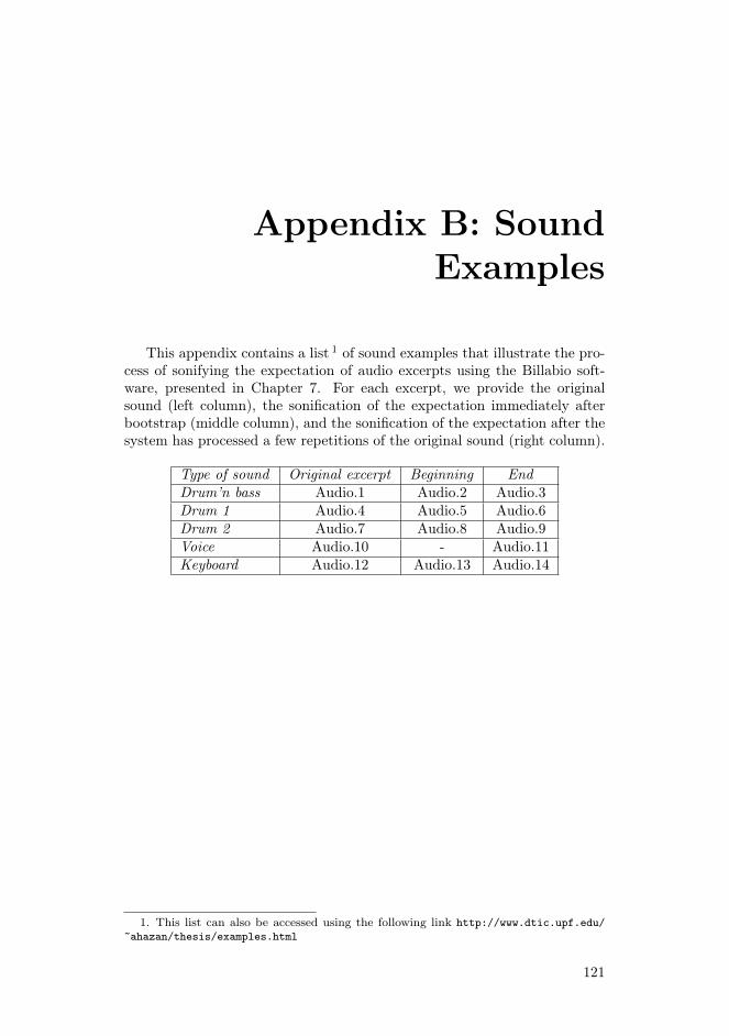
Appendix B: SoundExamples
This appendix contains a list 1 of sound examples that illustrate the pro-cess of sonifying the expectation of audio excerpts using the Billabio soft-ware, presented in Chapter 7. For each excerpt, we provide the originalsound (left column), the sonification of the expectation immediately afterbootstrap (middle column), and the sonification of the expectation after thesystem has processed a few repetitions of the original sound (right column).
Type of sound Original excerpt Beginning EndDrum’n bass Audio.1 Audio.2 Audio.3Drum 1 Audio.4 Audio.5 Audio.6Drum 2 Audio.7 Audio.8 Audio.9Voice Audio.10 - Audio.11Keyboard Audio.12 Audio.13 Audio.14
1. This list can also be accessed using the following link http://www.dtic.upf.edu/~ahazan/thesis/examples.html
121

This thesis has been written using LATEX
Copyright © 2022 FDOKUMEN