arX

iv:0

908.

1789

v2 [

cs.IT

] 25

Jun

201

01

Maximum-Likelihood Sequence Detector for

Dynamic Mode High Density Probe Storage

Naveen Kumar, Pranav Agarwal, Aditya Ramamoorthy and MurtiV. Salapaka

Abstract

There is an increasing need for high density data storage devices driven by the increased demand

of consumer electronics. In this work, we consider a data storage system that operates by encoding

information as topographic profiles on a polymer medium. A cantilever probe with a sharp tip (few

nm radius) is used to create and sense the presence of topographic profiles, resulting in a density of

few Tb per in.2. The prevalent mode of using the cantilever probe is the static mode that is harsh on

the probe and the media. In this article, the high quality factor dynamic mode operation, that is less

harsh on the media and the probe, is analyzed. The read operation is modeled as a communication

channel which incorporates system memory due to inter-symbol interference and the cantilever state.

We demonstrate an appropriate level of abstraction of this complex nanoscale system that obviates the

need for an involved physical model. Next, a solution to the maximum likelihood sequence detection

problem based on the Viterbi algorithm is devised. Experimental and simulation results demonstrate

that the performance of this detector is several orders of magnitude better than the performance of other

existing schemes.

I. INTRODUCTION

Present day high density storage devices are primarily based on magnetic, optical and solid

state technologies. Advanced signal processing and detection techniques have played an important

Naveen Kumar and Aditya Ramamoorthy are with Dept. of Electrical and Computer Engg. at Iowa State University, Ames IA

50011 (email:{nk3, adityar}@iastate.edu). Pranav Agarwal and Murti V. Salapaka are with the Dept. of Electrical and Computer

Engg. at University of Minnesota, Minneapolis, MN 55455 (email: {agar0108, murtis}@umn.edu). The material in this work

has appeared in part at IEEE GlobeCom 2009 and in part at CISS 2008.

June 28, 2010 DRAFT

role in the design of all data storage systems [24], [13], [4], [14], [15], [1], [10]. Indeed tech-

niques such as partial-response max-likelihood [4], [21],[24] were responsible for significantly

improving magnetic disk technology.

In this work, we consider a promising high density storage methodology which utilizes a sharp

tip at the end of a micro cantilever probe to create, remove and read indentations (see [22]). The

presence/absence of an indentation represents a bit of information. The main advantage of this

method is the significantly higher areal densities comparedto conventional technologies that are

possible. Recently, experimentally achieved tip radii near 5 nm on a micro-cantilever were used

to create areal densities close to 1 Tb/in2 [22].

A particular realization of a probe based storage device that uses an array of cantilevers, along

with the static mode operation is provided in [8]. However, there are fundamental drawbacks of

this technique. In the static mode operation, the cantilever is in contact with media throughout

the read operation which results in large vertical and lateral forces on the media and the tip.

Moreover, significant information content is present in thelow frequency region of the cantilever

deflection and it can be shown experimentally that the systemgain at low frequency is very

small. Therefore, in order to overcome the measurement noise at the output, the interaction

force between the tip and the medium has to be large. This degrades the medium and the probe

over time, resulting in reduced device lifetime.

The problem of tip and media wear can be partly addressed by using the dynamic mode

operation; particularly when a cantilever with a high quality factor is employed. In the dynamic

mode operation, the cantilever is forced sinusoidally using a dither piezo. The oscillating can-

tilever gently taps the medium and thus the lateral forces are reduced which decreases the media

wear [25]. Using cantilever probes that have high quality factors leads to high resolution, since

the effect of a topographic change on the medium on the oscillating cantilever lasts much longer

(approximatelyQ cantilever oscillation cycles, where each cycle is1/f0 seconds long andQ

andf0 is the quality factor and the resonant frequency of the cantilever respectively). Moreover,

the SNR improves as√Q [23]. However, this also results in severe inter-symbol-interference,

2

unless the topographic changes are spaced far apart. Spacing the changes far apart is undesirable

from the storage viewpoint as it implies lower areal density. Another issue is that the cantilever

exhibits complicated nonlinear dynamics. For example, if there is a sequence of hard hits on

the media, then the next hit results in a milder response, i.e., the cantilever itself has inherent

memory, that cannot be modeled as ISI. Conventional dynamicmode methods described in [17],

that utilize high-Q cantilevers are not suitable for data storage applications. This is primarily

because they are unable to deal with ISI and the nonlinear channel characteristics. The current

techniques can be considered analogous to peak detection techniques in magnetic storage [14].

In this work we demonstrate that these issues can be addressed by modeling the dynamic

mode operation as a communication system and developing high performance detectors for

it. Note that corresponding activities have been undertaken in the past for technologies such

as magnetic and optical storage [13], e.g., in magnetic storage, PRML techniques, resulted in

tremendous improvements. In our work, the main issues are, (a) developing a model for the

cantilever dynamics that predicts essential experimentalfeatures and remains tractable for data

storage purposes, and (b) designing high-performance detectors for this model, that allow the

usage of high quality cantilevers, without sacrificing areal density. As discussed in the sequel,

several concepts such as Markovian modeling of the cantilever dynamics and Viterbi detection

in the presence of noise with memory [1], play a key role in ourapproach.

Main Contributions:In this article, a dynamic mode read operation is researchedwhere the

probe is oscillated and the media information is modulated on the cantilever probe’s oscillations.

It is demonstrated that an appropriate level of abstractionis possible that obviates the need

for an involved physical model. The read operation is modeled as a communication channel

which incorporates the system memory due to inter-symbol interference and the cantilever

state that can be identified using training data. Using the identified model, a solution to the

maximum likelihood sequence detection problem based on theViterbi algorithm is devised.

Experimental and simulation results which corroborate theanalysis of the detector, demonstrate

that the performance of this detector is several orders of magnitude better than the performance

3

of other existing schemes and confirm performance gains thatcan render the dynamic mode

operation feasible for high density data storage purposes.

Our work will motivate research for fabrication of prototypes that are massively parallel and

employ high quality cantilevers (such as those used with thestatic mode [22] and intermittent

contact dynamic mode but with low-Q [5]). In current prototypes, the cantilever detection is

integrated into the cantilever structure and the cantilevers are actuated electrostatically. Even

though the experimental setup reported in this article usesa particular scheme for measuring the

cantilever detection and for actuating the cantilever, theparadigm developed for data detection

is largely applicable in principle to other modes of detection and actuation of the cantilever. The

analysis criteria primarily assume that high quality factor cantilevers are employed and that a

dynamic mode operation is pursued.

The article is organized as follows. In Section II, background and related work of the probe

based data storage system is presented. Section III deals with the problem of designing and

analyzing the data storage unit as a communication system and finding efficient detectors for

the channel model. Section IV and Section V report results from simulation and experiment

respectively. Section VI provides the main findings of this article and future work.

II. BACKGROUND AND RELATED WORK.

Probe based high density data storage devices employ a cantilever beam that is supported at

one end and has a sharp tip at another end as a means to determine the topography of the media

on which information is stored. The information on the mediais encoded in terms of topographic

profiles. A raised topographic profile is considered a high bit and a lowered topographic profile

is considered a low bit. There are various means of measuringthe cantilever deflection. In

the standard atomic force microscope setup, which has formed the basis of probe based data

storage, the cantilever deflection is measured by a beam-bounce method where a laser is incident

on the back of the cantilever surface and the laser is reflected from the cantilever surface into

a split photodiode. The photodiode collects the incident laser energy and provides a measure

of the cantilever deflection (see Figure 1(a)). The advantage of the beam-bounce method is

4

the high resolution (low measurement noise) and high bandwidth (in the 2-3 MHz) range. The

disadvantage is that it cannot be easily integrated into an operation where multiple cantilevers

operate in parallel. There are attractive measurement mechanisms that integrate the cantilever

motion sensing onto the cantilever itself. These include piezo-resistive sensing [3] and thermal

sensing [7]. For the dynamic mode operation there are various schemes to actuate the cantilever

that include electrostatic [5], mechanical by means of a dither piezo that actuates the support

of the cantilever base, magnetic [9] and piezoelectric [6].In this article, it is assumed that the

cantilever is actuated by a dither piezo and the sensing mechanism employed is the beam bounce

method (see Figure 1(a)).

A. Models of cantilever probe, the measurement process and the tip-media interaction

A first mode approximation of the cantilever is given by the spring mass damper dynamics

described by

p +ω0

Qp+ ω2

0p = f(t), y = p+ υ, (1)

where p = d2p

dt2, p, f, y and υ denote the deflection of the tip, the force on the cantilever,the

measured deflection and the measurement noise respectivelywhereas the parametersω0 andQ are

the first modal frequency (resonant frequency) and the quality factor of the cantilever respectively.

The input-output transfer function with inputf and outputp is given asG = 1s2+

ω0

Qs+ω2

0

. The

cantilever model described above can be identified precisely (see [18]).

The interaction force,h, between the tip and the media depends on the deflectionp of the

cantilever tip. Such a dependence is well characterized by the Lennard-Jones like force that is

typically characterized by weak long-range attractive forces and strong short range repulsive

forces (see Figure 1(c)). Thus, the probe based data storagesystem can be viewed as an

interconnection of a linear cantilever systemG with the nonlinear tip-media interaction forces

in feedback (see Figure 1(b) and note thatp = G(h+ η + g) with h = φ(p) [19]).

5

B. Cantilever-Observer Model

A state space representation of the filterG can be obtained asx = Ax + Bf, y = Cx + υ

wherex = [p p]T and f = η + g (assuming no media forcesh) andA, B andC are given by,

A =

0 1

−ω20 −ω0/Q

, B =

0

1

, C =

[

1 0

]

Based on the model of the cantilever, an observer to monitor the state of the cantilever can

be implemented [11] (see Figure 2). The observer dynamics and the associated state estimation

error dynamics is given by,

Observer︷ ︸︸ ︷

˙x = Ax+Bg + L(y − y); x(0) = x0,

y = Cx,

State Estimation Error Dynamics︷ ︸︸ ︷

˙x = Ax+B(g + η)−Ax−Bg − L(y − y),

= (A− LC)x+Bη − Lυ,

x(0) = x(0)− x(0),

whereL is the gain of the observer,x is the estimate of the statex andg is the external known

dither forcing applied to the cantilever. The error in the estimate is given byx = x− x, whereas

the error in the estimate of the outputy is given by,e = y− y = Cx+υ. The error between the

observed state and the actual state of the cantilever, when no noise terms or media forces are

present (η = υ = h = 0) is only due to the mismatch in the initial conditions of the observer and

the cantilever-tip. Note that the cantilever tip interactswith the media only for a small portion

of an oscillation. It is shown in [17] that such a tip-media interaction can be modeled well as an

impact force (in other words as an impulsive force) on the cantilever that translates into an initial

condition reset of the cantilever state. The error process is white if the Kalman gain is used for

L [11]. For cantilever deflection sensors with low enough and realizable levels of measurement

noise, the effective length of the impulse response of the system with media force as input and

the error signale as the output can be made as short as four periods of the cantilevers first

resonant frequency.

As described in [17], the discretized model of the cantilever dynamics is given by

xk+1 = Fxk +G(gk + ηk) + δθ,k+1ν , yk = Hxk + vk, k ≥ 0 , (2)

6

where the matricesF , G, andH are obtained from matricesA, B andC using the zero order

hold discretization at a desired sampling frequency andδi,j denotes the dirac delta function.θ

denotes the time instant when the impact between the cantilever tip and the media occurs andν

signifies the value of the impact. The impact results in an instantaneous change or jump in the

state byν at time instantθ. When a Kalman observer is used, the profile in the error signal due

to the media can be pre-calculated as,

ek = yk − yk = Γk;θ ν + nk , (3)

where{Γk;θ ν} is a known dynamic state profile with an unknown arrival timeθ defined by

Γk;θ = H(F − LKH)k−θ, for k ≥ θ. LK is the Kalman observer gain,nk is a zero mean

white noise sequence which is the measurement residual had the impact not occurred andθ is

assumed to be equal to 0 for simplicity. The statistics ofn are given by,E{njnTk } = V δjk where

V = HPxHT + R andPx is the steady state error covariance obtained from the Kalman filter

that depends onP andR which are the variances of the thermal noise and measurementnoise

respectively.

III. CHANNEL MODEL AND DETECTORS

A. Reformulation of state space representation

It is to be noted that although we have modeled the cantileversystem as a spring-mass-damper

model (second order system with no zeros and two stable poles)(see (1)), the experimentally

identified channel transfer function that is more accurate in practice has right half plane zeros

that are attributed to delays present in the electronics. Given this scenario, the state space

representation used in [17] leads to a discrete channel withtwo inputs as seen in (3) because the

structure ofB is no longer in the form of[0 1]T . However, source information enters the channel

as a single input as the tip-medium interaction force. The problem can be reformulated as one of

a channel being driven by a single input by choosing an appropriate state space representation.

For the state space model of the cantilever, it is known that the pair (A,B) is controllable

which implies there exists a transformation which will convert the state space into a controllable

7

canonical form such thatB = [0 1]T . This kind of structure ofB will force the discretized

model (2) to be such that one component ofν is equal to0. With B chosen as above, the entire

system can be visualized as a channel that has a single source. In this article, the single source

model is used as it simplifies the detector structure and analysis substantially.

B. Channel Model

The cantilever based data storage system can be modeled as a communication channel as

shown in Figure 3. The components of this model are explainedbelow in detail.

Shaping Filter (b(t)): The model takes as input the bit sequencea = (a0, a1 . . . aN−1) where

ak, k = 1, . . . , N −1 is equally likely to be 0 or 1. In the probe storage context, ‘0’ refers to the

topographic profile beinglow and ‘1’ refers to the topographic profile beinghigh. Each bit has a

duration ofT seconds. This duration can be found based on the length of thetopographic profile

specifying a single bit and the speed of the scanner. The height of the high bit is denoted byA.

The cantilever interacts with the media by gently tapping itwhen it is high. When the media

is low, typically no interaction takes place. We model the effect of the medium height using a

filter with impulse responseb(t) (shown in Figure 3) that takes as input, the input bit impulse

train a(t) =∑N−1

k=0 akδ(t− kT ). The output of the filter is given bya(t) =∑N−1

k=0 akb(t− kT ).

Nonlinearity Block (φ): The cantilever oscillates at frequencyf0 which means that in each

cantilever cycle of durationTc = 1/f0, the cantilever hits the media at most once if the media is

high during a timeTc. Due to the dynamics of the system it may not hit the media, even if it is

high. The magnitude of impact on the media is not constant andchanges according to the state

of the cantilever prior to the interaction with the media. Wenote that a very accurate modeling of

the cantilever trajectory will require the solution of complex nonlinear equations corresponding

to the cantilever dynamics and knowledge of the bit profile sothat each interaction is known. In

this work we model the impact values of the tip-media interaction by means of a probabilistic

Markov model that depends on the previous bits. This obviates the need for a detailed model.

We assume that in each high bit durationT , the cantilever hits the mediaq times (i.e.T = qTc)

with varying magnitudes. Therefore, forN bits, the output of the nonlinearity block is given by,

8

a(t) =∑Nq−1

k=0 νk(a)δ(t−kTc), whereνk denotes the magnitude of thekth impact of the cantilever

on the medium. Here, we approximate the nonlinearity block output as a sequence of impulsive

force inputs to the cantilever. The strength of the impulsive hit at any instant is dependent on

previous impulsive hits; precisely because the previous interactions affect the amplitude of the

oscillations that in turn affect how hard the hit is at a particular instance. The exact dependence

is very hard to model deterministically and therefore we chose a Markov model, as given below

for the sequence of impact magnitudes for a single bit duration,

νi = G(ai, ai−1, . . . , ai−m) + bi (4)

where νi = [νiq νiq+1 . . . ν(i+1)q−1]T and G(ai, ai−1, . . . , ai−m) is a function of the current and

the lastm bits. Herem denotes the system memory andbi is a zero mean i.i.d. Gaussian vector

of lengthq. The appropriateness of the model will be demonstrated by our experimental results.

Channel Response (Γ(t)): The Markovian modeling of the output of the nonlinearity block as

discussed above allows us to break the feedback loop in Figure 2 (see also [17]). The rest of

the system can then be modeled by treating it as a linear system with impulse responseΓ(t).

Γ(t) is the error between the cantilever tip deflection and the tipdeflection as estimated by the

observer when the cantilever tip is subjected to an impulsive force. It can be found in closed

form for a given set of parameters of cantilever-observer system (see (3)).

Channel Noise (n(t)): The measurement noise (from the imprecision in measuring the cantilever

position) and thermal noise (from modeling mismatches) canbe modeled by a single zero mean

white Gaussian noise process (n(t)) with power spectral density equal toV .

The continuous time innovation outpute(t) becomes,e(t) = s(t, ν(a))+n(t), wheres(t, ν(a)) =∑Nq−1

k=0 νk(a)Γ(t−kTc) and ν(a) = (ν0(a), ν1(a) . . . νNq−1(a)). The sequence of impact values

νi is assumed to follow a Markovian model as explained above,Γ(t) is the channel impulse

response andn(t) is a zero mean white Gaussian noise process.

9

C. Sufficient Statistics for Channel model

Before providing sufficient statistics we consolidate the notation used. The source stream is

N elements long (a denotes the sequence of source bits), with the topographic profile and the

scan speed is chosen such that the cantilever impacts any topographic profileq times. Thus there

areNq possible hits withν(a) denoting the sequence of strength of theNq impulsive hits on

the cantilever. Furthermore, the set of strengths of impulsive force inputs, which isq elements

long, during theith topographic profile encoding theith source symbol is denoted byνi. Given

the probabilistic model onν and finite bit sequence (a), an information lossless decomposition

of e(t) by expansion over an orthonormal finite-dimensional basis with dimensionN can be

achieved whereN orthonormal basis functions span the signal space formed bys(t, ν(a)). The

components ofe(t) over N orthonormal basis functions are given by,e = s(ν(a)) + n, where

e = (e0, e1 . . . eN), s(ν(a)) = (s0, s1 . . . sN), n = (n0, n1 . . . nN ) and n ∼ N(0, V IN×N)

whereIN×N stands forN × N identity matrix [10]. The maximum likelihood estimate of the

bit sequence can be found asˆa = argmaxa∈{0,1}N f(e|a) where ˆa = (a0, a1 . . . aN−1) is the

estimated bit sequence andf denotes a pdf. The termf(e|a) can be further simplified as,

f(e|a) =∫

ν

f(e|a, ν)f(ν|a)dν =

∫

ν

1

(2πV )N2

exp[−||e− s(ν(a))||2

2V]f(ν|a)dν

=1

(2πV )N2

exp−||e||22V

∫

ν

exp[−(||s(ν(a))||2 − 2eT s(ν(a)))

2V]f(ν|a)dν

where||.||2 denotes Euclidean norm,f(e|a, ν) andf(ν|a) denote the respective conditional pdf’s

andν = (ν0, ν1 . . . νNq−1). The correlation betweene ands(ν(a)) can be equivalently expressed

as an integral over time because of the orthogonal decomposition procedure i.e.eT s(ν(a)) =∫∞

−∞e(t)s(t, ν(a))dt = νT z′, where ν = (ν0, ν1 . . . νNq−1), z′ = (z′0, z′1 . . . z′Nq−1) and z′k =

∫∞

−∞e(t)Γ(t − kTc)dt for 0 ≤ k ≤ Nq − 1 is the output of a matched filterΓ(−t) with input

e(t) sampled att = kTc. The termf(e|a) can now be written as,

f(e|a) =1

(2πV )N2

exp−||e||22V

︸ ︷︷ ︸

h(e)

∫

ν

exp−||s(ν(a))||2

2Vexp

νT z′

Vf(ν|a)dν

︸ ︷︷ ︸

F(z′|a)

10

Sof(e|a) can be factorized intoh(e) (dependent only one) andF(z′|a) (for a givena dependent

only on z′). Using the Fisher-Neyman factorization theorem [2], we can claim thatz′ is a vector

of sufficient statistics for the detection process i.e.f(e|a)

f(z′|a)= C, whereC is a constant independent

of a. So we can reformulate the detection problem as,ˆa = argmaxa∈{0,1}N f(z′|a) which means

that bit detection problem depends only on the matched filteroutputs (z′). These matched filter

outputs for0 ≤ k ≤ Nq − 1 can be further simplified as,z′k =∑Nq−1

k1=0 νk1(a)h′k−k1

+ n′k, where

h′k−k1

=∫∞

−∞Γ(t − kTc)Γ(t − k1Tc)dt andn′

k =∫∞

−∞n(t)Γ(t − kTc)dt such thatE(n′

kn′k′) =

∫∞

−∞

∫∞

−∞E(n(t)n(τ))Γ(t−kTc)Γ(τ−k′Tc)dtdτ = V Rk−k′, whereRk−k′ =

∫∞

−∞Γ(t−kTc)Γ(t−

k′Tc)dt. A whitening matched filter can be determined to whiten output noisen′k [10]. We shall

denote the discretized output of whitened matched filter shown in Figure 4 aszk, such that

zk =∑I

k1=0 νk−k1(a)hk1 + nk, where the filter{hk}k=0,1,...,I denotes the effect of the whitened

matched filter and the sequence{nk} represents the Gaussian noise with varianceV .

D. Viterbi Detector Design

Note that the outputs of the whitened matched filterz, continue to remain sufficient statistics

for the detection problem. Therefore, we can reformulate the detection strategy as,

ˆa = arg maxa∈{0,1}N

f(z|a) = arg maxa∈{0,1}N

ΠN−1i=0 f(zi|a, zi−1

0 ) (5)

where z = [z0 z1 . . . zNq−1]T , zi is the received output vector corresponding to theith input

bit, i.e., zi = [ziq ziq+1 . . . z(i+1)q−1]T and zi−1

0 = [zT0 zT1 . . . zTi−1]T . In our model, the channel

is characterized by finite impulse response of lengthI i.e. hi = 0 for i < 0 and i > I and

we assume thatI ≤ mIq i.e. the inter-symbol-interference (ISI) length in terms of q hits is

equal tomI . Let m be the system memory (see (4)). The length of channel response is known

which means thatmI is known but the value ofm cannot be found because it depends on the

experimental parameters of the system. In the experimentalresults section, we describe how we

find the value ofm from experimental data. The received output vectorzi can now be written

11

as,

zi =

hI . . h0 0 . . 0

0 hI . . h0 0 . 0

. . . . . . . . . . . . .

0 . . 0 hI . . h0

νiq−I

ν1+iq−I

...

ν(i+1)q−1

+ ni = Hνii−mI

+ ni,

whereνi = [νiq νiq+1 . . . ν(i+1)q−1]T , νi

i−mI= [νT

i−mI. . . νT

i ]T andni = [niq n1+iq . . . n(i+1)q−1]

T .

Our next task is to simplify the factorization in (5) so that decoding can be made tractable.

We construct the dependency graph of the concerned quantities which is shown in Figure 5.

Using the Bayes ball algorithm [20], we conclude that

f(zi|νii−mI

, a, zi−10 ) = f(zi|νi

i−mI), (6)

f(νi−mI|a, zi−1

0 ) = f(νi−mI|ai−1

0 , zi−10 ), (7)

f(νi−k|νi−k−1i−mI

, a, zi−10 ) = f(νi−k|νi−k−1

i−mI, ai−mI−1

0 , ai−1i−k−m, z

i−10 ), ∀ 1 ≤ k ≤ mI − 1, (8)

f(νi|νi−1i−mI

, a, zi−10 ) = f(νi|aii−m), (9)

whereai−10 = [a0 a1 . . . ai−1]. Although the conditional pdff(νi−k|νi−k−1

i−mI, a, zi−1

0 ) and

f(νi−mI|a, zi−1

0 ) depend on the entire past, we assume that these dependenciesare rapidly

decreasing with increase in past time. This is observed in simulation and experimental data

as well. For making the detection process more tractable, wemake the following assumptions

on this dependence,

f(νi−mI|ai−1

0 , zi−10 ) ≈ f(νi−mI

|ai−1i−m−mI

, zi−1i−mI

), (10)

f(νi−k|νi−k−1i−mI

, ai−mI−10 , ai−1

i−k−m, zi−10 ) ≈ f(νi−k|νi−k−1

i−mI, ai−1

i−k−m, zi−1i−k), ∀ 1 ≤ k ≤ mI − 1, (11)

i.e. the dependence is restricted to only the immediate neighbors in the dependency graph. Using

12

the above assumptions and dependency graph results,f(zi|a, zi−10 ) can be further simplified as,

f(zi|a, zi−10 ) =

∫

f(zi|νii−mI

, a, zi−10 )f(νi

i−mI|a, zi−1

0 )dνii−mI

=

∫

f(zi|νii−mI

, a, zi−10 )f(νi−mI

|a, zi−10 )ΠmI−1

k=1 f(νi−k|νi−k−1i−mI

, a, zi−10 )f(νi|νi−1

i−mI, a, zi−1

0 )dνii−mI

=

∫

f(zi|νii−mI

)f(νi−mI|ai−1

0 , zi−10 )ΠmI−1

k=1 f(νi−k|νi−k−1i−mI

, ai−mI−10 , ai−1

i−k−m, zi−10 )

× f(νi|aii−m)dνii−mI

(Using (6), (7),(8),(9) )

=

∫

f(zi|νii−mI

)f(νi−mI|ai−1

i−m−mI, zi−1

i−mI)ΠmI−1

k=1 f(νi−k|νi−k−1i−mI

, ai−1i−k−m, z

i−1i−k)

× f(νi|aii−m)dνii−mI

(Using (10),(11))

=

∫

f(zi|νii−mI

, aii−m−mI, zi−1

i−mI)f(νi

i−mI|aii−m−mI

, zi−1i−mI

)dνii−mI

= f(zi|aii−m−mI, zi−1

i−mI).

By defining a stateSi = aii−m−mI+1, this can be further expressed asf(zi|Si, Si−1, zi−1i−mI

). Again

using Bayes ball algorithm, we conclude that

f(zii−mI|νi

i−2mI, aii−m−mI

) = f(zii−mI|νi

i−2mI), (12)

Π2mI−1k=1 f(νi−2mI+k|νi−2mI+k−1

i−2mI, aii−m−mI

) = ΠmI−1k=1 f(νi−2mI+k|νi−2mI+k−1

i−2mI, aii−m−mI

)

× Π2mI−1k=mI

f(νi−2mI+k|ai−2mI+ki−2mI+k−m), (13)

f(νi|νi−1i−2mI

, aii−m−mI) = f(νi|aii−m). (14)

The pdf of zii−mI= [zTi−mI

. . . zTi ]T given current stateSi and previous stateSi−1 is given by,

f(zii−mI|Si, Si−1) = f(zii−mI

|aii−m−mI) =

∫

f(zii−mI|νi

i−2mI, aii−m−mI

)f(νii−2mI

|aii−m−mI)dνi

i−2mI

=

∫

f(zii−mI|νi

i−2mI, aii−m−mI

)f(νi−2mI|aii−m−mI

)Π2mI−1k=1 f(νi−2mI+k|νi−2mI+k−1

i−2mI, aii−m−mI

)

× f(νi|νi−1i−2mI

, aii−m−mI)dνi

i−2mI=

∫

f(zii−mI|νi

i−2mI)f(νi−2mI

|aii−m−mI)ΠmI−1

k=1 f(νi−2mI+k|

νi−2mI+k−1i−2mI

, aii−m−mI)Π2mI−1

k=mIf(νi−2mI+k|ai−2mI+k

i−2mI+k−m)f(νi|aii−m)dνii−2mI

(Using (12),(13),(14))

where the last step is obtained using results from dependency graph and all the terms in the

last step exceptf(νi−2mI|aii−m−mI

) and ΠmI−1k=1 f(νi−2mI+k|νi−2mI+k−1

i−2mI, aii−m−mI

) are Gaussian

13

distributed. This implies that the pdf ofzii−mIgiven(Si, Si−1) is not exactly Gaussian distributed.

If the number of states in the detector is increased it can be modeled as a Gaussian which means

that the term likef(νi−2mI|aii−m−mI

) can be made Gaussian distributed by increasing the number

of states, but this increases the complexity. In order to keep the decoding tractable we make the as-

sumption thatf(zii−mI|Si, Si−1) is Gaussian i.e.f(zii−mI

|Si, Si−1) ∼ N(Y(Si, Si−1), C(Si, Si−1)),

whereY(Si, Si−1) is the mean andC(Si, Si−1) is the covariance. With our state definition, we can

reformulate the detection problem as a maximum likelihood state sequence detection problem [1],

ˆS = argmaxall S

f(z|S) = argmaxall S

ΠN−1i=0 f(zi|S, z0 . . . zi−1)

= argmaxall S

ΠN−1i=0 f(zi|Si, Si−1, z

i−1i−mI

) = argmaxall S

ΠN−1i=0

f(zii−mI|Si, Si−1)

f(zi−1i−mI

|Si, Si−1)

= argminall S

N−1∑

i=0

[log(|C(Si, Si−1)||c(Si, Si−1)|

) + (zii−mI− Y(Si, Si−1))

TC(Si, Si−1)−1

× (zii−mI− Y(Si, Si−1))− (zi−1

i−mI− y(Si, Si−1))

T c(Si, Si−1)−1(zi−1

i−mI− y(Si, Si−1))]

where ˆS is estimated state sequence,c(Si, Si−1) is the uppermIq × mIq principal minor of

C(Si, Si−1) and y(Si, Si−1) collects the firstmIq elements ofY(Si, Si−1). It is assumed that

the first state is known. With metric given above, Viterbi decoding can be applied to get the

maximum likelihood state sequence and the corresponding bit sequence.

E. LMP, GLRT and Bayes Detector

In [17], the hit detection algorithm is proposed which ignores the modeling of channel memory

and works well only when the hits are sufficiently apart. In [12], various detectors for hit detection

like locally most powerful (LMP), generalized likelihood ratio test (GLRT) and Bayes detector

are presented. These detectors also ignore the system memory and perform detection of single

hits. Subsequently a majority type rule is used for bit detection. The continuous time innovation

(e(t)) is sampled at very high sampling rate1/Ts such thatTs << Tc. As the channel response

(Γ(t)) is finite length, the sampled channel response is assumed tohave the finite length equal

to M . The sampled channel response is given by,

Γ0 = [Γ(t)|t=0 Γ(t)|t=Ts. . . Γ(t)|t=(M−1)Ts

]T

14

Determining when the cantilever is “hitting” the media and when it is not, is formulated as a

binary hypothesis testing problem with the following hypotheses,

H0 : e = n, H1 : e = Γ0ν + n

where the sampled innovation vectore = [e1 e2 . . . eM ]T , n = [n1 n2 . . . nM ]T , Γ0 is the sampled

channel response,ν signifies the value of the impact on media andV IM×M denotes the covariance

matrix of n whereIM×M stands forM ×M identity matrix. In case of locally most powerful

(LMP) test given in [16], the likelihood ratio is given by [12],

llmp(M) =∂

∂ν(log

f(e|H1)

f(e|H0))|ν=0 = eTV −1Γ0.

where llmp denotes likelihood ratio for LMP. In our model, there areq number of hits in one

bit duration. Letlk,lmp be the likelihood ratio corresponding tokth hit. The decision rule for the

detection of one bit in this case is defined as,

Max

(

l1,lmp(M) , l2,lmp(M) . . . lq,lmp(M)

)

≶01 τ1 (15)

whereτ1 is LMP threshold. The likelihood ratio in the case of GLRT is [12],

lglrt(M) = logf(e|H1, ν = ν)

f(e|H0)= l2lmp,

whereν is maximum likelihood (ML) estimate ofν i.e. ν = argmaxν f(e|H1), llmp andlglrt are

likelihood ratios for LMP and GLRT case respectively. The decision rule for the bit detection

in this case is defined in a similar manner given in (15).

Simulations from a Simulink model of the system can be run fora large number of hits in

order to gather statistics on the discretized output of nonlinearity block which models the tip-

media force. We modeled the statistics forν by a Gaussian pdf with the appropriate mean and

variance. With known mean and variance ofν the likelihood ratio for Bayes test is [12],

lbayes(M) = logf(e|H1)

f(e|H0)= eTV −1µ′ +

1

2eTV ′e− eTV ′µ′,

whereµ′ = Γ0α andV ′ =Γ0ΓT

0

(V2

λ2+V ΓT

0Γ0)

andν ∼ N(α, λ2). The decision rule in this case is also

defined in a similar manner given in (15). Note thatν is a measure of the tip-medium interaction

15

force and as such it is difficult to experimentally verify thevalue of this force accurately which

means the Bayes test cannot be applied for the bit detection on actual experimental data.

IV. SIMULATION RESULTS

We performed simulations with the following parameters. The first resonant frequency of the

cantileverf0 = 63.15 KHz, quality factor Q =206, the value of forcing amplitude equal to 24 nm,

tip-media separation is 28 nm, the number of hits in high bit duration is equal to13 i.e. q = 13,

discretized thermal and measurement noise variance are0.1 and 0.001 respectively. A Kalman

observer was designed and the length of the channel impulse response (I) was approximately

24 which means thatmI is equal to2. We set the value of the system memory,m = 1. Using

a higher value ofm results in a more complex detector. We used a topographic profile where

high and low regions denote bits ‘1’ and ‘0’ respectively andthe bit sequence is generated

randomly. The simulation was performed with the above parameters using the Simulink model

that mimics the experimental station that provides a qualitative as well as a quantitative match

to the experimental data. Tip-media interaction was variedby changing the height of media

corresponding to bit ‘1’. We define the system SNR as the nominal tip-media interaction (nm)

divided by total noise variance.

In Figure 6, we compare the results of four different detectors. The LMP, GLRT and Bayes

detector perform hit detection, as against bit detection. In these detectors, the system memory is

not taken into account. It is clear that the minimum probability of error for all detectors decreases

as the tip-media interaction increases which makes SNR higher. The intuition behind this result

is that hits become harder on media if tip-media interactionis increased which makes detection

easier. The Viterbi detector gives best performance among all detectors because it incorporates

the Markovian property ofν in the metric used for detection. At an SNR of 10.4 dB the Viterbi

detector has a BER of3× 10−6 as against the LMP detector that has7× 10−3.

V. EXPERIMENTAL RESULTS

In experiments, a cantilever with resonant frequencyf0 = 71.78 KHz and quality factor

Q = 67.55 is oscillated near its resonant frequency. A freshly cleaved mica sheet is placed on

16

top of a high bandwidth piezo. This piezo can position the media (mica sheet) in z-direction with

respect to cantilever tip. A random sequence of bits is generated through an FPGA board and

applied to the z-piezo. High level is equivalent to1 V and represents bit ‘1’ and low level is0 V

and represents bit ‘0’ thus creating a pseudo media profile of6 nm height. The bit width can be

changed using FPGA controller from60−350 µs. The tip is engaged with the media at a single

point and its instantaneous amplitude in response to its interaction with z piezo is monitored.

The controller gain is kept sufficiently low such that the operation is effectively in open loop.

The gain is sufficient to cancel piezo drift and maintain a certain level of tip-media interaction.

An observer is implemented in another FPGA board which is based on the cantilever’s free air

model and takes dither and deflection signals as its input andprovides innovation signal at the

output. The innovation signal is used to detect bits by comparing various bit detection algorithms.

The experiments were performed on Multimode AFM, from VeecoInstruments. Considering a

bit width of 40 nm and scan time of60 µs gives a tip velocity equal to2/3× 10−3 m/sec. The

total scan size of the media is 100 micron which means the cantilever will take 0.15 seconds to

complete one full scan. Read scan speed for this operation is6.66 Hz. The read scan speed for

different bit widths can be found in a similar manner.

The cantilever model is identified using the frequency sweepmethod wherein excitation

frequencyω of g(t) = A0 sinωt of dither piezo is varied from0 − 100 KHz and p(t) is

recorded. Magnitude and phase information aboutG(iω) is obtained by evaluating the ratios

between steady state amplitude and phase of output vs input excitation respectively. A second

order transfer function is obtained that best fits the experimentally identified magnitude and phase

responses of the cantilever.A, B andC matrices are obtained from the state space realization

of the identified second order transfer function.F , G and H can be further found using the

zero order hold discretization at a desired sampling frequency. The discretized state space of the

cantilever model is used to find the discretized channel impulse responseΓk;θ (see (3)).

For 300 µs bit width, there are around21 hits in high bit duration and Viterbi decoding

is applied on the innovation signal obtained from experiment. For experimental model,I is

17

approximately24 which meansmI is equal to2. It is hard to estimate the system memory

(m) from experimental parameters. Fortunately, there is a wayaround for this. As shown in

the derivation of the detector, by making appropriate approximations, the final detector only

requires the mean and the covariance of each branch in the trellis. These can be found by using

training data and assuming various values ofm. We have variedm from 0 to 2 and found the

corresponding BER using these values ofm. The total number of states in the Viterbi detector

is 2m+mI . We have observed that form > 1, the improvement in BER is quite marginal as

compared to the increased complexity of Viterbi decoding. Accordingly we are usingm = 1

for which the BER from Viterbi decoding is equal to1 × 10−5 whereas the BER from LMP

test is0.26. The BER in the case of Viterbi decoding is significantly smaller when compared to

the BER for usual thresholding detectors. If the bit width isdecreased to60 µs which means

there are around4 hits in the high bit duration, the BER for Viterbi decoding is7.56 × 10−2

whereas the BER for LMP is0.49 which means that LMP is doing almost no bit detection. As

the bit width is decreased, there is more ISI between adjacent bits which increases the BER.

The BER for different bit widths from all the detectors is shown in Figure 8. It can be clearly

seen that Viterbi decoding gives remarkable results on experimental data as compared to the

LMP detector. The Viterbi detector exploits the cantileverdynamics by modeling the mean and

covariance matrix for different state transitions. We haveplotted the mean vectors for2 state

transitions with300 µs bit width in Figure 7. There are around21 hits in one bit duration.

The Viterbi decoding contains8 states and16 possible state transitions. In Figure 7, there is a

clear distinction in mean vectors for different transitions which makes the Viterbi detector quite

robust. Thresholding detectors like LMP and GLRT perform very badly on experimental data.

For a bit sequence like ‘000011111’, the cantilever gets enough time to go into steady state in

the beginning and hits quite hard on media when bit ‘1’ appears after a long sequence of ‘0’

bits. The likelihood ratio for LMP and GLRT rises significantly for such high bits which can

be easily detected through thresholding. However, a sequence of continuous ‘1’ bits keeps the

18

cantilever in steady state with the cantilever hitting the media mildly which means the likelihood

ratio remains small for these bits. Thus it is very likely that long sequence of ‘1’ bits will not

get detected by threshold detectors.

VI. CONCLUSIONS AND FUTURE WORK

We presented the dynamic mode operation of a cantilever probe with a high quality factor and

demonstrated its applicability to a high-density probe storage system. The system is modeled as

a communication system by modeling the cantilever interaction with media. The bit detection

problem is solved by posing it as a ML sequence detection followed by Viterbi decoding. The

main requirements for the proposed algorithm are (a) the availability of training sequences which

can provide the statistics for different state transitions, (b) differences between the tip-media

interaction magnitude between ‘0’ and ‘1’ bit and (c) an accurate characterization of the linear

model of the cantilever in free air. Simulation and experimental results show that the Viterbi

detector outperforms LMP, GLRT and Bayes detector and givesremarkably low BER. The work

reported in this article demonstrates that competitive metrics can be achieved and enables probe

based high density data storage, where high quality factor probes can be used in the dynamic

mode operation. Thus, it alleviates the issues of media and tip wear in previous probe based

data storage systems.

An efficient error control coding system is a must for any datastorage system since the sector

error rate specifications are on the order of10−10 for systems in daily use such as hard drives.

In future work, we are expecting to achieve this BER by using appropriate coding techniques.

Using run-length-limited (RLL) codes in our system is likely to improve performance and we

shall examine this issue in future work. We are also working on a BCJR version of the algorithm

to minimize the BER of the system even further. In experimental data, a small amount of jitter

is inevitably present which is well handled by our algorithm. At high densities, the jitter will be

significantly higher and we will need to apply more advanced modeling and detection techniques.

These are part of ongoing and future work.

19

REFERENCES

[1] Kavcic Aleksandar and Jose M. F. Moura. The Viterbi Algorithm and Markov Noise Memory.IEEE Trans. on Info. Th.,

46 , Issue: 1:291–301, 2000.

[2] G. Casella and R. Berger.Statistical Inference. Duxbury Thomson Learning, second edition, 2002.

[3] B.W. Chui, H.J. Mamin, B.D. Terris, D. Rugar, and T.W. Kenny. Sidewall-implanted dual-axis piezoresistive cantilever

for afm data storage readback and tracking. InMicro Electro Mechanical Systems, 1998. MEMS 98. Proceedings., The

Eleventh Annual International Workshop on, pages 12–17, Jan 1998.

[4] R.D. Cideciyan, F. Dolivo, R. Hermann, W. Hirt, and W. Schott. A PRML system for digital magnetic recording.IEEE

Journal on Selected Areas in Communications, 10(1):38–56, Jan 1992.

[5] P. Baechtold A. Sebastian H. Pozidis D. R. Sahoo, W. Haeberle and E. Eleftheriou. On intermittent-contact mode sensing

using electrostatically-actuated micro-cantilevers with integrated thermal sensors.Proceeding of the American Control

Conference, pages 2034 – 2039, June 2008.

[6] D.L. DeVoe and A.P. Pisano. Modeling and optimal design of piezoelectric cantilever microactuators.Journal of

Microelectromechanical Systems, 6(3):266–270, Sep 1997.

[7] U. Durig. Fundamentals of micromechanical thermoelectric sensors.Journal of Applied Physics,, 98:044, 2005.

[8] E. Eleftheriou, T. Antonakopoulos, G.K. Binnig, G. Cherubini, M. Despont, A. Dholakia, U. Durig, M.A. Lantz, H. Pozidis,

H.E. Rothuizen, and P. Vettiger. Millipede - a mems-based scanning-probe data-storage system.IEEE Transactions on

Magnetics, 39(2):938–945, Mar 2003.

[9] E. Eleftheriou et al. A nanotechnology-based approach to data storage. InVLDB ’2003: Proceedings of the 29th

international conference on Very large data bases, pages 3–7. VLDB Endowment, 2003.

[10] Jr. Forney, G. Maximum-likelihood sequence estimation of digital sequences in the presence of intersymbol interference.

IEEE Trans. on Info. Th., 18 , Issue: 3:363 – 378, 1972.

[11] T. Kailath, A. H. Sayed, and B. Hassibi.Linear Estimation. Prentice Hall, 2000.

[12] N. Kumar, P. Agarwal, A. Ramamoorthy, and M. Salapaka. Channel modeling and detector design for dynamic mode high

density probe storage. In42nd Conference on Information Sciences and Systems. IEEE, 2008.

[13] J. Moon. The role of sp in data-storage systems.IEEE Signal Processing Magazine, 15(4):54–72, Jul 1998.

[14] J. Moon and L.R. Carley. Performance comparison of detection methods in magnetic recording.IEEE Transactions on

Magnetics, 26(6):3155–3172, Nov 1990.

[15] Jaekyun Moon and Jongseung Park. Pattern-dependent noise prediction in signal-dependent noise.IEEE Journal on

Selected Areas in Communications, 19(4):730–743, Apr 2001.

[16] H. Vincent Poor. An Introduction to Signal Detection and Estimation, 2nd Ed.Springer-Verlag, 1994.

[17] D. R. Sahoo, A. Sebastian, and M. V. Salapaka. Harnessing the transient signals in atomic force microscopy.International

Journal of Robust and Nonlinear Control, Special Issue on Nanotechnology and Micro-biology, 15:805–820, 2005.

[18] M. V. Salapaka, H. S. Bergh, J. Lai, A. Majumdar, and E. McFarland. Multi-mode noise analysis of cantilevers for scanning

probe microscopy.Journal of Applied Physics, 81(6):2480–2487, March 1997.

20

[19] A. Sebastian, M. V. Salapaka, D. Chen, and J. P. Cleveland. Harmonic and power balance tools for tapping-mode atomic

force microscope.Journal of Applied Physics, 89 (11):6473–6480, June 2001.

[20] R. D. Shachter. Bayes-Ball: The Rational Pastime (for Determining Irrelevance and Requisite Information in Belief

Networks and Influence Diagrams) . InUncertainty in Artificial Intelligence: Proceedings of theFourteenth Conference,

pages 480–487, 1998.

[21] H. Thapar and A. Patel. A class of partial response systems for increasing storage density in magnetic recording.IEEE

Transactions on Magnetics, 23(5):3666–3668, Sep 1987.

[22] P. Vettiger, G. Cross, M. Despont, U. Drechsler, U. Durig, B. Gotsmann, W. Haberele, M. A. Lantz, H. Rothuizen, R. Stutz,

and G. Binnig. The millipede-nanotechnology entering datastorage.IEEE Transactions on Nanotechnology, 1((1)), 2002.

[23] R. Wisendanger.Scanning Probe Microscopy and Spectroscopy. Cambridge University Press, 1994.

[24] R. Wood and D. Petersen. Viterbi detection of class IV partial response on a magnetic recording channel.IEEE Transactions

on Communications, 34(5):454–461, May 1986.

[25] Q. Zhong, D. Inniss, K. Kjoller, and V B Elings. Fractured polymer/silica fiber surface studied by tapping mode atomic

force microscopy.Surface Science Letters, 290:L688–L692, 1993.

21

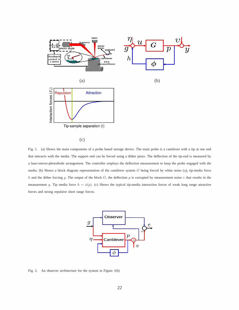
(a) (b)

(c)

Fig. 1. (a) Shows the main components of a probe based storagedevice. The main probe is a cantilever with a tip at one end

that interacts with the media. The support end can be forced using a dither piezo. The deflection of the tip-end is measuredby

a laser-mirror-photodiode arrangement. The controller employs the deflection measurement to keep the probe engaged with the

media. (b) Shows a block diagram representation of the cantilever systemG being forced by white noise (η), tip-media force

h and the dither forcingg. The output of the blockG, the deflectionp is corrupted by measurement noiseυ that results in the

measurementy. Tip media forceh = φ(p). (c) Shows the typical tip-media interaction forces of weak long range attractive

forces and strong repulsive short range forces.

Fig. 2. An observer architecture for the system in Figure 1(b)

22

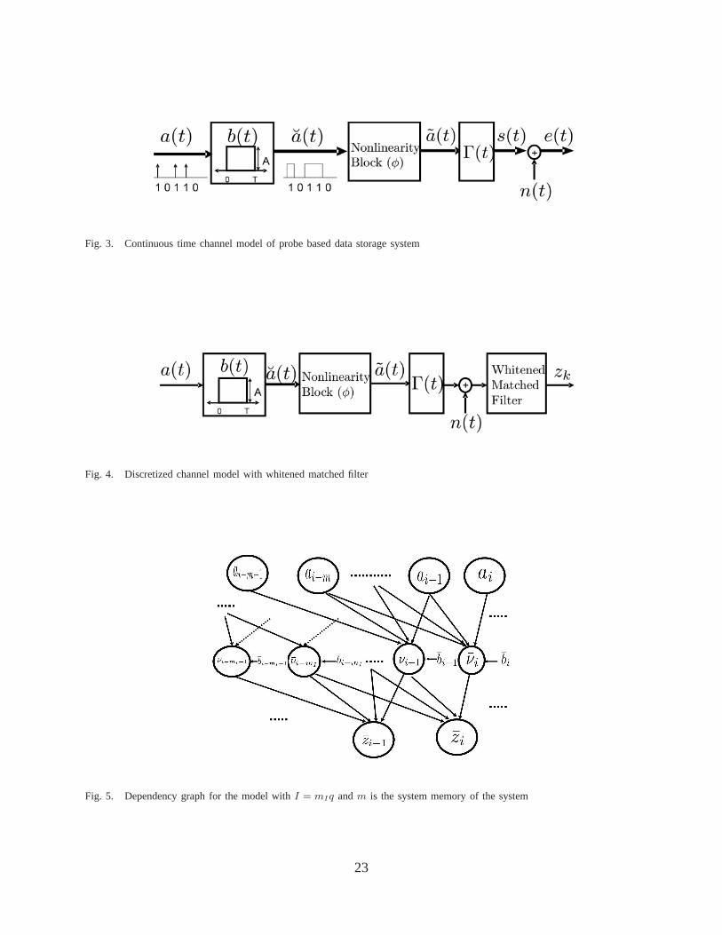
Fig. 3. Continuous time channel model of probe based data storage system

Fig. 4. Discretized channel model with whitened matched filter

Fig. 5. Dependency graph for the model withI = mIq andm is the system memory of the system

23

Fig. 6. Comparison of various detectors for simulation data. The Bayes curve is not visible in the graph as it coincides with

the LMP curve.

Fig. 7. Mean vector for2 state transitions for300 µs bit width from experimental data where ‘1100’ and ‘1101’ represents

transition from state ‘110’ to state ‘100’ and ‘101’ respectively

24

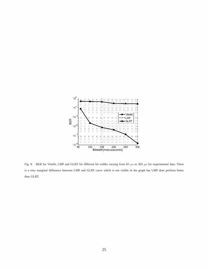
Fig. 8. BER for Viterbi, LMP and GLRT for different bit widthsvarying from60 µs to 300 µs for experimental data. There

is a very marginal difference between LMP and GLRT curve which is not visible in the graph but LMP does perform better

than GLRT.

25