Statistics and Probability Letters 79 (2009) 2158–2165

Contents lists available at ScienceDirect

Statistics and Probability Letters

journal homepage: www.elsevier.com/locate/stapro

Maximum likelihood parameter estimation for the multivariateskew–slash distributionOlcay Arslan ∗Department of Statistics, Cukurova University, 01330 Balcalı, Adana, Turkey

a r t i c l e i n f o

Article history:Received 13 January 2009Received in revised form 3 July 2009Accepted 6 July 2009Available online 18 July 2009

MSC:62F1062H12

a b s t r a c t

In this paper we consider the parameter estimation of the multivariate skew–slashdistribution introduced by Arslan [Arslan, O. 2008. An alternative multivariate skew–slashdistribution. Statistics and Probability Letters 78, 2756–2761], which is a recent example ofthe normal variance–mean mixture distributions. Due to the complexity of the likelihoodfunction, estimation of its parameters by direct maximization of the likelihood functionseems difficult. To overcome this problem, we propose a simple EM-based maximumlikelihood estimation procedure to estimate the parameters of themultivariate skew–slashdistribution. We provide three examples to demonstrate the modeling strength of themultivariate skew–slash distribution and the feasibility of the proposed EM algorithm.

© 2009 Elsevier B.V. All rights reserved.

1. Introduction

Scale mixtures of normal distributions, which have been very popular in robust statistical analysis for analyzing heavy-tailed datasets, assume that the variance is not fixed for all members of the population. However, in some cases, wemay notonly have the problemof non-constant variance, but alsomay have that the variance is related to themean. To dealwith suchproblems the scalemixtures of normal distributions have been extended to the normal variance–meanmixture distributions(Barndorff-Nielsen, 1977, 1978; Blaesild, 1981; Barndorff-Nielsen et al., 1982; McNeil et al., 2005). The idea behind thevariance–mean mixture distributions is to introduce randomness into the variance and mean of a normal distribution via apositivemixing variable. Normal variance–meanmixture distributions attempt to add some asymmetry to the scalemixtureof normal distributions. They are more flexible and can provide useful asymmetric and heavy-tailed extensions of theirsymmetric counterparts for robust statistical modeling of datasets involving distributions with heavy tails and skewness.A recent example of the normal variance–mean mixture distributions is the multivariate skew–slash distribution

introduced by Arslan (2008), which is defined as the variance–mean mixture of the multivariate normal and the betadistributions.

Definition 1 (Multivariate Skew–Slash Distribution). Let Z ∼ Np(0, Ip

)with p ≥ 1, and V ∼ beta(λ, 1), with the density

function f (v) = λvλ−1, λ > 0 on (0, 1), be two independent random variables, and define a p-dimensional random variableX as

X = µ+ V−1β +√

V−1Σ1/2Z, (1)

where µ, β ∈ Rp,Σ is a positive definite matrix, andΣ1/2 is the square root ofΣ . Then, X is said to have a p-dimensionalskew–slash distribution (X ∼ SSp(µ,Σ, β, λ)) with the density function

∗ Tel.: +90 322 3386084; fax: +90 322 338 6070.E-mail address: oarslan@cu.edu.tr.

0167-7152/$ – see front matter© 2009 Elsevier B.V. All rights reserved.doi:10.1016/j.spl.2009.07.009

O. Arslan / Statistics and Probability Letters 79 (2009) 2158–2165 2159

f (x;µ,Σ, β, λ) = Ce(x−µ)TΣ−1β

{∫ 1

0tλ+

p2−1e−

12

[ts+t−1βTΣ−1β

]dt}

=

C(√βTΣ−1β

)λ+ p2e(x−µ)

TΣ−1βKλ+ p2

(√s

√βTΣ−1β

;√s(βTΣ−1β)

)(√s)λ+ p2 , x 6= µ, β 6= 0

C∫ 1

0

(tλ+

p2−1e−

12

[t−1βTΣ−1β

])dt, x = µ, β 6= 0

C2

2λ+ p, x = µ, β = 0

(2)

where x ∈ Rp, s = (x− µ)TΣ−1(x− µ), C = λ|Σ |−1/2

(2π)p/2is the normalizing constant, and Ka (δ; b) =

∫ δ0 ta−1e−

b2 (t+t

−1)dt, a ∈R, b > 0, is the incomplete modified Bessel function of third kind (Jones, 2007).

As seen from the definition the shape of the multivariate skew–slash density is specified by one scalar parameter λ,two vector parameters µ and β and one matrix parameter Σ . These parameters have natural explanations relating to theoverall shape of the density function as follows. The parameter λ controls the tail tackiness of the density, in the sense thatlarge values of λ imply light tails, while smaller values of λ imply heavier tails. The parameter β is a vector of skewnessparameters, the parameterµ is a vector of location parameters, and the parameterΣ is the positive definite scatter matrix.In practice, the condition |Σ | = 1 is imposed on Σ to avoid an unidentifiable scale factor. With these parameters, themultivariate skew–slash distribution becomes a flexible member of the normal variance–meanmixture distribution family,and it provides an alternative model in analyzing skewed datasets with heavy tails in which the normal distribution wouldnot be appropriate.If X ∼ SSp(µ,Σ, β, λ), then the conditional distribution of X given V = v is Np(µ+v−1β, v−1Σ) and the characteristic

function of X has the form ΨX (t) = eitTµEV

[e−V

−1(tTΣt/2−itTβ)]. Further, because Z and V are independent the moments of

X ∼ SSp(µ,Σ, β, λ) follow immediately from the moments of Z and E(V−r

)=

λλ−r , λ > r . In particular, the expectation

and the variance of X are given by

E(X) = µ+λ

λ− 1β, λ > 1, (3)

Var(X) =λ

λ− 1Σ +

λ

(λ− 2)(λ− 1)2ββT, λ > 2. (4)

When β = 0 the random variable X has the multivariate slash distribution which is a member of the elliptical family. Onecan see Lange and Sinsheimer (1993),Wang and Genton (2006), Gomez et al. (2007), and Arslan and Genc (2009a) for furtherdetails about the multivariate slash distribution.In this paper, we mainly discuss the parameter estimation of the multivariate skew–slash distribution, which is not

treated in detail in Arslan (2008). The conventional way of estimating the parameters of the multivariate skew–slashdistribution is to use the maximum likelihood estimation method. However, due to the complexity of the likelihoodfunction, the estimation of the parameters of the multivariate skew–slash distribution by direct maximization of thelikelihood function is a difficult task. To overcome this difficulty, we use the advantage of the variance–mean mixturerepresentation given in (1), and propose a simple EM based maximum likelihood parameter estimation procedure toestimate its parameters. The EM algorithm is a powerful algorithm for maximum likelihood estimation for data containingmissing values. It is particularly used for the maximum likelihood parameter estimation of the mixture distributions, sincethe mixing variable can be considered as missing data.The paper is organized as follows. Section 2 provides the EM-based maximum likelihood estimation procedure and a

simple iteratively reweighting algorithm to compute the maximum likelihood estimates. In Section 3 we analyze three realdatasets, and fit these to themultivariate skew–slashmodel, wherewe apply the proposed parameter estimation algorithm.We finalize the paper with a conclusion section.

2. Parameter estimation

Assume that we have i.i.d. data x1, x2, . . . , xn in Rp and wish to fit a multivariate skew–slash (SSp(µ,Σ, β, λ))distribution with the unknown parameters µ,Σ, β and λ. The log-likelihood function that we want to maximize is

l(µ,Σ, β, λ) = n ln λ−n2ln |Σ | +

n∑i=1

(xi − µ)TΣ−1β

+

n∑i=1

ln{∫ 1

0tλ+

p2−1e−

12

[t(xi−µ)TΣ−1(xi−µ)+t−1(βTΣ−1β)

]dt}. (5)

2160 O. Arslan / Statistics and Probability Letters 79 (2009) 2158–2165

We can see that direct maximization of this function seems not very easy to obtain the maximum likelihood estimators forthe parameters. But, the normal variance–meanmixture representation of themultivariate skew–slash distribution providesa great advantage to apply the EM algorithm to find the maximum likelihood estimators for the parameters of interest.The idea of the EM algorithm is to assume that the latentmixing variables V1, V2, . . . , Vn from themixture representation

in (1) are also observable. Let (xi, Vi), for i = 1, 2, . . . , n, be the complete data, where xi and Vi are called the observed dataand missing data, respectively. Since the joint density of X and V is given by

f (x, v) =(λ |Σ |−1/2

(2π)p/2

)vλ+

p2−1e(x−µ)

TΣ−1βe−12

[vs+v−1(βTΣ−1β)

]. (6)

The log-likelihood function for the complete data (xi, Vi), for i = 1, 2, . . . , n, up to an additive constant, can be constructedas

L(µ,Σ, β, λ) = n ln λ−n2ln |Σ | +

n∑i=1

(xi − µ)TΣ−1β −12

n∑i=1

Vi(xi − µ)TΣ−1(xi − µ)

−12βTΣ−1β

(n∑i=1

V−1i

)+

(λ+

p2− 1

) n∑i=1

ln Vi. (7)

Comparing with the actual likelihood function given in (5), the maximization of the complete data log-likelihood functionwith respect to µ,Σ, β and λ will be relatively easy. However, in reality, V is a latent variable and we cannot observe it. Itmeans that the estimators obtained bymaximizing L(µ,Σ, β, λ)will depend on V andwe cannot use them sincewe cannotobserve V . To overcome the latency of V wewill take the conditional expectation of L(µ,Σ, β, λ) given the observed data xiand the current estimates for the parameters, say, µ, Σ, β and λ. After taking the conditional expectation of L(µ,Σ, β, λ)we get

Q (µ,Σ, β, λ) = E(L(µ,Σ, β, λ) | xi, µ, Σ, β, λ)

= n ln λ−n2ln |Σ | +

n∑i=1

(xi − µ)TΣ−1β −12

n∑i=1

E(Vi|xi, µ, Σ, β, λ)(xi − µ)TΣ−1(xi − µ)

−12βTΣ−1β

n∑i=1

E(V−1i |xi, µ, Σ, β, λ)+(λ+

p2− 1

) n∑i=1

E(ln Vi|xi, µ, Σ, β, λ), (8)

where E(Vi|xi, µ, Σ, β, λ), E(V−1i |xi, µ, Σ, β, λ) and E(ln Vi|xi, µ, Σ, β, λ) are the conditional expectations of Vi, V−1i and

ln Vi given the observed data xi and the current estimates of the parameters. To find these conditional expectations we needthe conditional distribution of V given X . Before exploring the conditional distribution of V given X , let us first introducethe following distribution.

Definition 2 (Incomplete Generalized Inverse Gaussian Distribution). A positive random variable V defined on (0, 1) is said tohave an Incomplete Generalized Inverse Gaussian distribution (V ∼ IGIG(a, ψ, χ)) if its probability density function takesthe form

f (v) =

(√ψ

χ

)ava−1e−

12

[ψv+χv−1

]Ka(√

ψ

χ;√ψχ

) , (9)

where 0 < v < 1, a ∈ R, ψ, χ > 0, and Ka(√

ψ

χ;√ψχ

)=∫ √ψ

χ

0 ta−1e−√ψχ2 (t+t−1)dt is the incomplete modified Bessel

function of third kind.

The moments of the random variable V ∼ IGIG(a, ψ, χ) are

E(V k) =

(√ψ

χ

)k Ka+k (√ψ

χ;√ψχ

)Ka(√

ψ

χ;√ψχ

) . (10)

After some straightforward algebra, it is shown that the conditional distribution of V given X is an IGIG distribution withthe following density function

fV |X (v) =(√

sβTΣ−1β

)λ+ p2 vλ+p2−1e−

12

[sv+(βTΣ−1β)v−1

]

Kλ+ p2

(√s

βTΣ−1β;√(βTΣ−1β)s

) , (11)

O. Arslan / Statistics and Probability Letters 79 (2009) 2158–2165 2161

where 0 < v < 1, and the parameters are a = λ +p2 , ψ = s, and χ = βTΣ−1β , respectively. Using this conditional

distribution we get

wi = E(Vi|xi, µ, Σ, β, λ)

=

√βTΣ−1β√si

Kλ+ p2+1(√

siβTΣ−1β

;

√(βTΣ−1β)si

)Kλ+ p2

(√si

βTΣ−1β;

√(βTΣ−1β)si

) (12)

ui = E(V−1i |xi, µ, Σ, β, λ)

=

√si√

βTΣ−1β

Kλ+ p2−1(√

siβTΣ−1β

;

√(βTΣ−1β)si

)Kλ+ p2

(√si

βTΣ−1β;

√(βTΣ−1β)si

) (13)

ηi = E(ln Vi|xi, µ, Σ, β, λ)

=

( √si√

βTΣ−1β

)λ+ p2Kλ+ p2

(√si

βTΣ−1β;

√(βTΣ−1β)si

) ∫ 1

0(ln v)vλ+

p2−1e−

12

[siv+(βTΣ−1β)v−1

]dv, (14)

where si = (xi − µ)TΣ−1(xi − µ), for i = 1, 2, . . . , n. If the conditional expectations E(Vi|xi, µ, Σ, β, λ),E(V−1i |xi, µ, Σ, β, λ) and E(ln Vi|xi, µ, Σ, β, λ) are replaced by wi, ui and ηi we get the following objective function tobe maximized

Q (µ,Σ, β, λ) = n ln λ−n2ln |Σ | +

n∑i=1

(xi − µ)TΣ−1β −12

n∑i=1

wi(xi − µ)TΣ−1(xi − µ)

−12βTΣ−1β

n∑i=1

ui +(λ+

p2− 1

) n∑i=1

ηi. (15)

Taking the derivatives of Q (µ,Σ, β, λ)with respect to the parameters µ,Σ, β and λ and setting them equal to zero yieldthe following estimators

β =ave {wi (x− xi)}ave {wi} ave {ui} − 1

(16)

µ =ave {wixi} − βave {wi}

(17)

Σ = ave{wi(xi − µ)(xi − µ)T

}− ave {ui} ββT (18)

λ = −1

ave{ηi}. (19)

where, ave{.} stands for the average over i = 1, 2, . . . , n and x = ave{xi}.A general description of a single iteration of the EM algorithm can be given as follows:

• E-Step: Given xi and the current parameter estimates, find the conditional expectation of the log-likelihoodfunction given in (7). This corresponds to calculating the conditional expectations wi = E(Vi|xi, µ, Σ, β, λ), ui =E(V−1i |xi, µ, Σ, β, λ) and ηi = E(ln Vi|xi, µ, Σ, β, λ) in Q (µ,Σ, β, λ).• M-Step: Maximize Q (µ,Σ, β, λ) with respect to µ,Σ, β and λ to obtain the new estimates. This step corresponds toupdating the parameter values using the conditional expectations calculated in the E-step and the updating equationsgiven in Eqs. (16)–(19).

These two steps of the EM algorithm can be formulated as the following simple iteratively reweighting algorithm tocalculate the maximum likelihood estimates of the parameters. The algorithm is iterated until a reasonable convergencecriterion is reached. This algorithm can be easily implemented and the convergence is guaranteed since it is an EMalgorithm.However, if the likelihood function has several local extreme points the EM algorithm may be trapped in a local extremepoint. This problem can be solved by choosing appropriate initial points, or by repeating the algorithm several times withdifferent initial points.

2162 O. Arslan / Statistics and Probability Letters 79 (2009) 2158–2165

Iteratively reweighting algorithm1. Set iteration number k = 1 and select initial estimates for the parameters µ,Σ, β and λ.2. Using the current estimates µ(k),Σ (k), β(k) and λ(k) for k = 1, 2, 3, . . . , and the equations given in (12)–(14) calculatethe weightsw(k)i , u

(k)i and η

(k)i for i = 1, 2, . . . , n, and find the averages ave{w

(k)i }, ave{u

(k)i } and ave{η

(k)i }.

3. Use the following updating equations to calculate the new estimates β(k+1), µ(k+1),Σ (k+1) and λ(k+1)

β(k+1) =ave

{w(k)i (x− xi)

}ave

{w(k)i

}ave

{u(k)i

}− 1

µ(k+1) =ave

{w(k)i xi

}− β(k+1)

ave{w(k)i

}Λ = ave

{w(k)i (xi − µ

(k+1))(xi − µ(k+1))T}− ave

{u(k)i

}β(k+1)(β(k+1))T

Σ (k+1)= Λ/ |Λ|1/p

λ(k+1) = −1

ave{η(k)i }.

4. Repeat these steps until convergence.

For the symmetric case set β(k+1) = 0 and compute µ(k+1),Σ (k+1) and λ(k+1).

3. Examples

In this section we will analyze three real-world datasets and fit these to the multivariate skew–slash distributions. Weprovide these examples to demonstrate the modeling strength of the skew–slash distribution and the feasibility of theproposed EM-based maximum likelihood parameter estimation.

Example 1 (cDNA Microarray Datasets). In our first example we consider the cDNAmicroarray datasets of the NCI60 cancercell lines which are available at the web site http://discover.nci.nih.gov/datasetsNature2000.jsp. The cDNA microarraydatasets consist of several observations measured on the 60 human cancer cell (NCI60) lines. More details about thesedatasets can be found at the web site given above. We will consider the gene expression dataset. These dataset containsmeasurements of 1376 gene expression levels on the 60 human cancer cells and called the ‘‘T-Matrix’’ with the dimension1376 × 60. Each column of this matrix represents one cancer cell line. We consider this dataset as we were inspired bythe ideas of Purdom and Holmes (2005) who proposed to use a univariate skew Laplace distribution to model a similarmicroarray dataset.We consider each column of thismatrix separately as a univariate dataset.We observe that the empiricaldistribution of each column mostly appears to be asymmetric, peaky and heavy-tailed. Therefore, the distribution of eachcolumn can be well approximated by a skew heavy-tailed distribution. Arslan (2009) used a univariate skew Laplacedistribution to model one of the columns (named CO:KM12), and observed that the skew Laplace distribution capturesthe peak at the center of the data as well as the skewness and the heavy tails.

In this paper, we consider two columns of the T-Matrix (columns OV:SK.OV.3 and CO:KM12) as two different univariatedatasets, and fit a univariate skew–slash distribution to each of these columns to demonstrate that the univariate skew–slashdistribution can also be used as an alternative distribution to model such datasets. The maximum likelihood estimationprocedure described in this paper yields the maximum likelihood estimates µ = 0.369, and σ = 0.539, β = −0.141and λ = 1.072 for OV:SK.OV.3, and µ = 2.019, σ = 0.766, β = −1.552 and λ = 2.381 for CO:KM12. Fig. 1 depicts thehistograms and the fitted skew–slash densities for these datasets. We observe that the univariate skew–slash distributioncaptures the peak at the center of the data as well as the skewness and the heavy tails, and hence presents adequate fits tothe data.

Example 2 (MartinMarietta Data). This example considers the data taken fromButler et al. (1990). This dataset consists of 60monthly observations from January 1982 to December 1986. For this dataset a linear regressionmodel y = β0+β1CRSP+εis introduced, where y is the excess rate of the Martin Marietta company, CRSP is an index of the excess rate of return forthe New York market and ε is an error term. The fitted line obtained from the ordinary least squares is yOLS = 0.0011 +1.803CRSP . Butler et al. (1990) assumed that ε has a generalized t (GT ) distribution and obtained the regression estimates.The same dataset was considered by Lye andMartin (1993), Azzalini and Capitanio (2003), DiCiccio andMonti (2004), ArslanandGenc (2009b), andArslan (2009). In all of these papers itwas assumed that the error termhas a skewdistribution, such as,skew t , skew exponential power, skew generalized t , and skew Laplace distributions. Azzalini and Capitanio (2003) assumedthat ε has a skew t distribution and obtained the fitted line ySEP = 0.0029+1.248CRSP , DiCiccio andMonti (2004) assumedthat ε has a skew exponential power distribution and obtained the fitted line yST = −0.0807 + 1.304CRSP, and Arslan(2009) assumed that ε has a skew Laplace distribution and obtained the fitted line ySL = −0.0027+ 1.252CRSP.

O. Arslan / Statistics and Probability Letters 79 (2009) 2158–2165 2163

Fig. 1. Histograms and fitted skew–slash densities for the gene expression data considered in Example 1. Columns OV:SK.OV.3 (left) and CO:KM12 (right).

Fig. 2. Martin Marietta data. Scatter plot and fitted regression lines (left). Histogram of the residuals obtained from the skew–slash regression line and thefitted skew–slash density (right).

In this paper we assume that ε ∼ SS1(0, σ 2, β, λ), or, equivalently, y | CRSP ∼ SS1(β0 + β1CRSP, σ 2, β, λ). Weobtain the following maximum likelihood estimates with the standard errors given in brackets β0 = −0.096(0.06),β1 = 1.239(0.223), σ = 0.045(0.009), and λ = 2.543(0.528). Since we assume a skew–slash distribution as an errordistribution E(y | CRSP) = β0 + β1CRSP + E(ε), and hence the fitted line obtained from the skew–slash distributionis given by ySS = β0 + E(ε) + β1CRSP = 0.005 + 1.239CRSP, where E(ε) is the mean of the fitted error distribution.Fig. 2 shows the scatter plot of the data with the fitted lines obtained from the ordinary least squares, the skew t (Azzaliniand Capitanio, 2003), and skew–slash distributions. From this figure we observe that the fitted lines obtained from theskew–slash distribution and the skew t distribution are very close. Fig. 2 also displays the histogram of the residuals rSS andthe fitted skew–slash density function. This plot indicates that there is a satisfactory agreement between the observed dataand the fitted distribution.

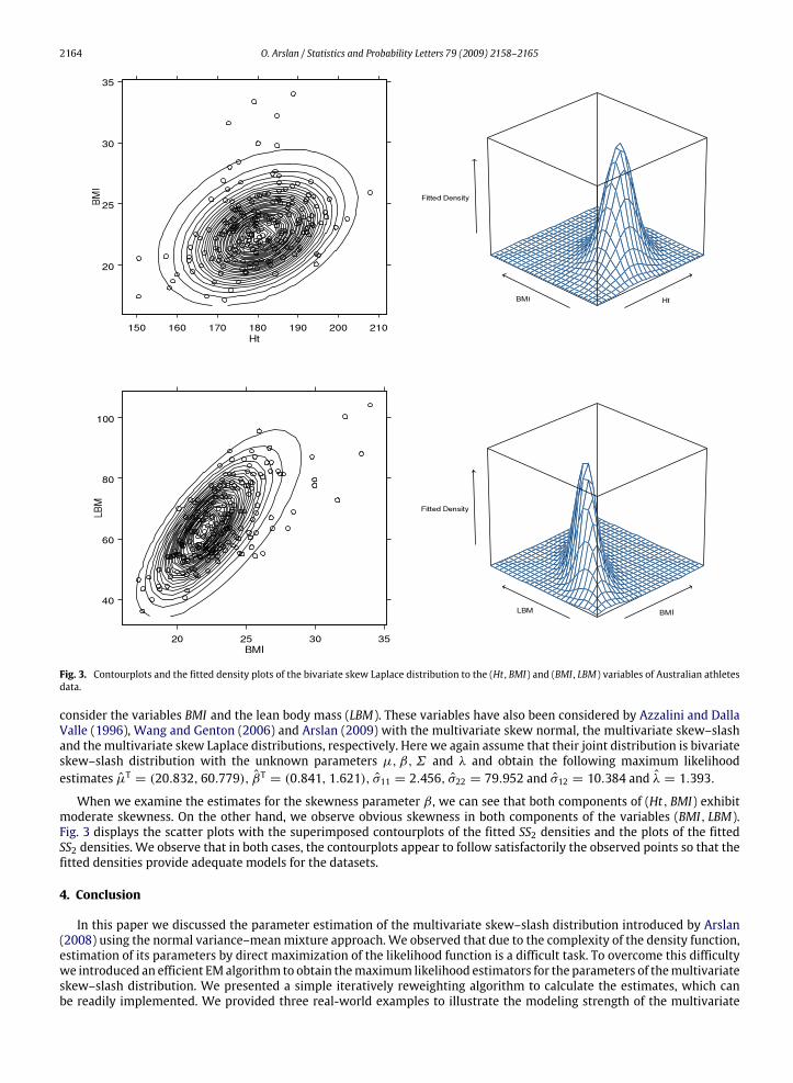
Example 3 (Australian Athletes Data). In our final example we will use the Australian athletes dataset analyzed by Azzaliniand Dalla Valle (1996), Azzalini and Capitanio (2003), Genton (2004), Wang and Genton (2006), and Arslan (2009). Thedataset contains several variables measured on 202 athletes. We will first consider the variables height (Ht) and body massindex (BMI). The same variables have also been analyzed by Genton (2004) and Arslan (2009) with the flexible skew normaldistribution (FGSN) and the skew Laplace distribution (MSL2), respectively. We fit a bivariate skew–slash (SS2) distributionto this dataset with the unknown parameters µ, β,Σ and λ. The maximum likelihood estimates of the parameters areµT = (181.327, 21.612), βT = (−0.562, 0.617), σ11 = 51.158, σ22 = 3.203 and σ12 = 5.095 and λ = 1.691. Next we

2164 O. Arslan / Statistics and Probability Letters 79 (2009) 2158–2165

Fig. 3. Contourplots and the fitted density plots of the bivariate skew Laplace distribution to the (Ht , BMI) and (BMI , LBM) variables of Australian athletesdata.

consider the variables BMI and the lean body mass (LBM). These variables have also been considered by Azzalini and DallaValle (1996), Wang and Genton (2006) and Arslan (2009) with the multivariate skew normal, the multivariate skew–slashand the multivariate skew Laplace distributions, respectively. Here we again assume that their joint distribution is bivariateskew–slash distribution with the unknown parameters µ, β,Σ and λ and obtain the following maximum likelihoodestimates µT = (20.832, 60.779), βT = (0.841, 1.621), σ11 = 2.456, σ22 = 79.952 and σ12 = 10.384 and λ = 1.393.

When we examine the estimates for the skewness parameter β , we can see that both components of (Ht, BMI) exhibitmoderate skewness. On the other hand, we observe obvious skewness in both components of the variables (BMI, LBM).Fig. 3 displays the scatter plots with the superimposed contourplots of the fitted SS2 densities and the plots of the fittedSS2 densities. We observe that in both cases, the contourplots appear to follow satisfactorily the observed points so that thefitted densities provide adequate models for the datasets.

4. Conclusion

In this paper we discussed the parameter estimation of the multivariate skew–slash distribution introduced by Arslan(2008) using the normal variance–meanmixture approach. We observed that due to the complexity of the density function,estimation of its parameters by direct maximization of the likelihood function is a difficult task. To overcome this difficultywe introduced an efficient EMalgorithm to obtain themaximum likelihood estimators for the parameters of themultivariateskew–slash distribution. We presented a simple iteratively reweighting algorithm to calculate the estimates, which canbe readily implemented. We provided three real-world examples to illustrate the modeling strength of the multivariate

O. Arslan / Statistics and Probability Letters 79 (2009) 2158–2165 2165

skew–slash distribution for handling skewness and heavy tails and the feasibility of the proposed EM algorithm. We foundthat the skew–slash distributions captured peakedness at center, skewness andheavy-tailedness in these datasetswith greataccuracy. We believe that, after solving the estimation problem of its parameters, the multivariate skew–slash distributionwill prove to be an alternative for modeling of datasets involving with skewness, peakedness and heavy-tailedness.

Acknowledgements

The author would like to thank an anonymous referee and the editor for their helpful comments and suggestions whichimproved this paper.

References

Arslan, O., 2008. An alternative multivariate skew–slash distribution. Statistics and Probability Letters 78, 2756–2761.Arslan, O., Genc, A.I., 2009a. The skew generalized t distribution as a scalemixture of the skew exponential power distribution and its applications in robuststatistical analysis, Statistics, in press, (doi:10.1080/02331880802401241).

Arslan, O., Genc, A.I., 2009b. A generalization of the multivariate slash distribution. Journal of Statistical Planning and Inference 139, 1164–1170.Arslan, O., 2009. An alternative multivariate skew Laplace distribution: Properties and estimation, Statistical papers, in press, (doi:10.1007/s00362-008-0183-7).

Azzalini, A., Dalla Valle, A., 1996. The multivariate skew–normal distribution. Biometrika 83, 715–726.Azzalini, A., Capitanio, A., 2003. Distributions generated by perturbation of symmetry with emphasis on a multivariate skew t distribution. Journal of theRoyal Statistical Society, Series B 65, 367–389.

Barndorff-Nielsen, O., 1977. Exponentially decreasing distributions for logarithmof particle size. Proceedings of the Royal Society of LondonA353, 401–419.Barndorff-Nielsen, O., 1978. Hyperbolic distributions and distributions on hyperbolae. Scandinavian Journal of Statistics 9, 43–46.Barndorff-Nielsen, O., Kent, J., Sorensen, M., 1982. Normal variance-mean mixtures and z distributions. International Statistical Review 50, 145–159.Blaesild, P., 1981. The two-dimensional hyperbolic distribution and related distributions, with an application to Johannsen’ bean data. Biometrika 68,251–263.

Butler, R.J., McDonald, J.B., Nelson, R.D., White, S.B., 1990. Robust and partially adaptive estimation of regression models. The Review of Economics andStatistics 72, 321–327.

DiCiccio, T.J., Monti, A.C., 2004. Inferential aspects of the skew exponential power distribution. Journal of the American Statistical Association 99, 439–450.Genton,M.G., 2004. Skew–Elliptical Distributions and Their Applications: A JourneyBeyondNormality. Chapman&Hall/CRC, Boca Raton, FL, Edited, Volume.Gomez, H.W., Quintana, A., Torres, J., 2007. A new family of slash-distributions with elliptical contours. Statistics and Probability Letters 77, 717–725.Jones, D.S., 2007. Incomplete Bessel functions I. Proceedings of the Edinburgh Mathematical Society 50, 173–183.Lange, K., Sinsheimer, J.S., 1993. Normal/Independent distributions and their applications in robust regression. Journal of Computational and GraphicalStatistics 2, 175–198.

Lye, J.N., Martin, V.L., 1993. Robust estimation, nonnormalities, and generalized exponential distributions. Journal of the American Statistical Association88, 261–267.

McNeil, A., Frey, R., Embrechts, P., 2005. Quantitative Risk Management: Concepts, Techniques and Tools. Princeton University Press.Purdom, E., Holmes, S.P., 2005. Error distribution for gene expression data. Statistical Applications in Genetics and Molecular Biology, 4, Article 16.http://www.bepress.com/sagmb.

Wang, J., Genton, M.G., 2006. The multivariate skew–slash distribution. Journal of Statistical Planning and Inference 136, 209–220.